Embed Size (px)
Citation preview

STUDIES ON
OPIMIZATION MODELS
OF FINANCIAL AND REAL OPTIONS
MICHI NISHIHARA


STUDIES ON
OPIMIZATION MODELS
OF FINANCIAL AND REAL OPTIONS
MICHI NISHIHARA


STUDIES ON
OPIMIZATION MODELS
OF FINANCIAL AND REAL OPTIONS
by
MICHI NISHIHARA
Submitted in partial fulfillment of
the requirement for the degree of
DOCTOR OF INFORMATICS
KYOTO UNIVERSITY
(Applied Mathematics and Physics)
NOVEMBER 2007


Preface
In this thesis, I study problems concerning both financial and real options in stochastic finance.
As well-known, option pricing theory has originated from the Black-Scholes model in 1970s. In
the model, Black, Scholes, and Merton proposed the concept of no-arbitrage pricing and derived
theoretical prices of call and put options in closed forms. These studies gave deep impact to
practitioners working around the Wall Street. Option pricing theory brought about the revolution
in the field of financial engineering, since portfolio optimization proposed by Markowitz in 1950s.
Option pricing theory still continues to develop for thirty years since the Black-Sholes model. While
countless stochastic models which are much more complicated and sophisticated have been proposed
up to now, this thesis contributes toward studies on option pricing from an opposite angle. In fact,
this thesis conducts option pricing based on prices of other derivative securities without assuming
any stochastic differential equation models.
In 1980s, the idea of option pricing began to be applied to evaluation of other things such as
developing natural resources beyond pricing conventional derivative securities. After that, in 1990s,
the word real options studies, which represent studies applying option pricing techniques to more
general decision making, has become increasingly popular. At present, real options studies which
are combined with other theory such as game theory, contract theory, and theory of optimal capital
structure play an important role in corporate finance. Furthermore, in practice, many consulting
firms utilize the idea of real options for resolving managerial matters.
Such active studies and rapid spread of real options will bring about the third revolution in the
history of financial engineering. This third revolution will be shared among much more people than
those in the previous revolutions. That is, real options methods are widely directed to all kinds of
decision makers in all kinds of organizations, rather than restricted specialists in investment insti-
tutions. I hope that this thesis helps both researchers and practitioners to understand effectiveness
of the real options approach.

vi Preface
Michi Nishihara
November 2007

Acknowledgment
First of all, I would like to express my sincere appreciation to Professor Masao Fukushima of Kyoto
University, who supervised me throughout my doctoral course. Although I have often troubled him,
he kindly supported me, read my draft manuscripts carefully, and gave me precise and detailed
advices. Without his generous support, this thesis could not have been accomplished. Also, his
eager and earnest attitude to the studies as a researcher is respectable. I would like to bear such
a spirit in my mind, and attempt to improve not only my technical skills of research but also my
mentality facing up to difficulties.
Second, I would also like to express my gratitude to Professor Toshihide Ibaraki of Kwansei
Gakuin University, Professor Mutsunori Yagiura of Nagoya University, and Professor Hiroshi Nag-
amochi of Kyoto University, who supervised me during my master course. Although I was one of
typical students who were too confident to notice their ignorance at that time, they gave me op-
portunities to determine the research subject and conduct research freely. Without their tolerance,
I would never start the studies on options in stochastic finance. During the guidance, they gave me
many hints in obtaining some results on option pricing based only on the no-arbitrage assumption
in this thesis.
I would also like to tender my acknowledgments to Professor Masaaki Kijima of Tokyo Metropoli-
tan University. Since the second grade in my master course, I have learned a fundamental of fi-
nancial engineering at his seminars. Whenever I had an opportunity to present my work at his
seminar, he suggested many ideas that greatly improved the work. Some results on real options in
this thesis were motivated and supported by the participants of his seminars as well as him.
Fortunately, I had valuable opportunities to discuss the related studies with many other re-
searchers. The discussion always helped me to broaden my horizons and bring new insight about
the studies. Above all, Professor Masamitsu Ohnishi of Osaka University, Professor Motoh Tsu-
jimura of Ryukoku University, Professor Takashi Shibata of Tokyo Metropolitan University, and
Atuyuki Ohyama, who is a doctoral course student of Kyoto University, gave me useful comments

viii Contents
and suggestions. In addition, I would like to thank all the members of Professor Fukushima’s
Laboratory, Professor Kijima’s Laboratory, Professor Nagamochi’s Laboratory (formerly Professor
Ibaraki’s Laboratory) of Kyoto University, and the Center for the Study of Finance and Insurance,
Osaka University for their generous support.
It was also fortunate for me that many funds supported my research. Actually, my studies were
partially supported by the Ministry of Education, Culture, Sports, Science and Technology (MEXT)
under Grant-in-Aids for the 21st Century COE Programs “Informatics Research Center for Devel-
opment of Knowledge Society Infrastructure” and “Interfaces for Advanced Economic Analysis”.
The Ishii Memorial Securities Research Promotion Foundation also supported my studies.
Finally, I would like to dedicate this thesis to my parents with my appreciation for their warm-
hearted support.

Contents
Preface v
Acknowledgment vii
List of Figures xiii
List of Tables xv
1 Introduction 1
1.1 Financial options . . . . . . . . . . . . . . . . . . . . . . . . . . . . . . . . . . . . . . 1
1.2 Real options . . . . . . . . . . . . . . . . . . . . . . . . . . . . . . . . . . . . . . . . . 2
1.3 Overview of the thesis . . . . . . . . . . . . . . . . . . . . . . . . . . . . . . . . . . . 4
2 Option Pricing Based on Prices of Other Derivatives: Duality 7
2.1 Introduction . . . . . . . . . . . . . . . . . . . . . . . . . . . . . . . . . . . . . . . . . 7
2.2 Preliminaries . . . . . . . . . . . . . . . . . . . . . . . . . . . . . . . . . . . . . . . . 8
2.3 Financial interpretation of duality . . . . . . . . . . . . . . . . . . . . . . . . . . . . 11
2.3.1 A buy-and-hold hedging portfolio . . . . . . . . . . . . . . . . . . . . . . . . . 11
2.3.2 Financial interpretation of duality of the SIP . . . . . . . . . . . . . . . . . . 12
2.4 Conclusion . . . . . . . . . . . . . . . . . . . . . . . . . . . . . . . . . . . . . . . . . 15
3 Option Pricing Based on Prices of Other Derivatives: Risk-Neutral Probabilities 17
3.1 Introduction . . . . . . . . . . . . . . . . . . . . . . . . . . . . . . . . . . . . . . . . . 17
3.2 Problem formulation . . . . . . . . . . . . . . . . . . . . . . . . . . . . . . . . . . . . 18
3.3 Bounds on risk-neutral measures . . . . . . . . . . . . . . . . . . . . . . . . . . . . . 20
3.4 Computational results . . . . . . . . . . . . . . . . . . . . . . . . . . . . . . . . . . . 24
3.5 Conclusion . . . . . . . . . . . . . . . . . . . . . . . . . . . . . . . . . . . . . . . . . 28
x Contents
4 Real Options Involving Alternative Investment Projects 31
4.1 Introduction . . . . . . . . . . . . . . . . . . . . . . . . . . . . . . . . . . . . . . . . . 31
4.2 Single firm situation . . . . . . . . . . . . . . . . . . . . . . . . . . . . . . . . . . . . 34
4.3 Situation of two noncooperative firms . . . . . . . . . . . . . . . . . . . . . . . . . . 38
4.3.1 Case where the leader has invested in technology 2 . . . . . . . . . . . . . . 40
4.3.2 Case where the leader has invested in technology 1 . . . . . . . . . . . . . . . 43
4.4 Analysis in two typical cases . . . . . . . . . . . . . . . . . . . . . . . . . . . . . . . . 44
4.4.1 De facto standard case . . . . . . . . . . . . . . . . . . . . . . . . . . . . . . . 45
4.4.2 Innovative case . . . . . . . . . . . . . . . . . . . . . . . . . . . . . . . . . . . 47
4.4.3 Case of joint investment . . . . . . . . . . . . . . . . . . . . . . . . . . . . . . 51
4.5 Numerical examples . . . . . . . . . . . . . . . . . . . . . . . . . . . . . . . . . . . . 52
4.6 Conclusion . . . . . . . . . . . . . . . . . . . . . . . . . . . . . . . . . . . . . . . . . 55
5 Real Options under Incomplete Information 61
5.1 Introduction . . . . . . . . . . . . . . . . . . . . . . . . . . . . . . . . . . . . . . . . . 61
5.2 Model . . . . . . . . . . . . . . . . . . . . . . . . . . . . . . . . . . . . . . . . . . . . 62
5.3 Case of complete information . . . . . . . . . . . . . . . . . . . . . . . . . . . . . . . 64
5.4 Loss due to incomplete information . . . . . . . . . . . . . . . . . . . . . . . . . . . . 69
5.4.1 The start-up’s strategy under incomplete information . . . . . . . . . . . . . 69
5.4.2 The real expected payoff of the start-up . . . . . . . . . . . . . . . . . . . . . 73
5.4.3 The start-up’s loss due to incomplete information . . . . . . . . . . . . . . . . 74
5.5 General setting . . . . . . . . . . . . . . . . . . . . . . . . . . . . . . . . . . . . . . . 77
5.6 Numerical examples . . . . . . . . . . . . . . . . . . . . . . . . . . . . . . . . . . . . 78
5.7 Conclusion . . . . . . . . . . . . . . . . . . . . . . . . . . . . . . . . . . . . . . . . . 81
6 Real Options under Asymmetric Information 85
6.1 Introduction . . . . . . . . . . . . . . . . . . . . . . . . . . . . . . . . . . . . . . . . . 85
6.2 Preliminaries . . . . . . . . . . . . . . . . . . . . . . . . . . . . . . . . . . . . . . . . 86
6.3 Theoretical results . . . . . . . . . . . . . . . . . . . . . . . . . . . . . . . . . . . . . 89
6.4 Economic insights . . . . . . . . . . . . . . . . . . . . . . . . . . . . . . . . . . . . . 94
6.5 Conclusion . . . . . . . . . . . . . . . . . . . . . . . . . . . . . . . . . . . . . . . . . 96
7 Conclusion 97

Contents xi
A Appendix of Chapter 4 99
A.1 The stopping time game and its equilibrium . . . . . . . . . . . . . . . . . . . . . . . 99


List of Figures
2.1 Buy-and-hold hedging portfolios. . . . . . . . . . . . . . . . . . . . . . . . . . . . . . 15
3.1 Convexity of call option prices. . . . . . . . . . . . . . . . . . . . . . . . . . . . . . . 21
3.2 Meanings of αi, γi, li. . . . . . . . . . . . . . . . . . . . . . . . . . . . . . . . . . . . . 22
3.3 Prices of Nikkei-225 call options on March 11, 2004, with the exercise date of April
8, 2004. . . . . . . . . . . . . . . . . . . . . . . . . . . . . . . . . . . . . . . . . . . . 25
3.4 fmax(a) and fmin(a) on April 8, 2004. . . . . . . . . . . . . . . . . . . . . . . . . . . . 27
3.5 fmax(a) and fmin(a) on different dates in 2004. . . . . . . . . . . . . . . . . . . . . . . 29
4.1 (Firm 1’s cash flow, Firm 2’s cash flow). . . . . . . . . . . . . . . . . . . . . . . . . . 39
4.2 The value function M(Y ) in the single firm case. . . . . . . . . . . . . . . . . . . . . 48
4.3 The leader’s payoff L(Y ) and the follower’s payoff F (Y ). . . . . . . . . . . . . . . . . 48
4.4 The monopolist’s value function M(Y ). . . . . . . . . . . . . . . . . . . . . . . . . . 56
4.5 Li(Y ) and Fi(Y ) in the de facto standard case. . . . . . . . . . . . . . . . . . . . . . 56
4.6 L(Y ), F (Y ) and J(Y ) in the de facto standard case. . . . . . . . . . . . . . . . . . . 57
4.7 L(Y ), F (Y ) and J(Y ) for σ = 0.8 in the de facto standard case. . . . . . . . . . . . . 57
4.8 Li(Y ) and Fi(Y ) in the innovative case. . . . . . . . . . . . . . . . . . . . . . . . . . 58
4.9 L(Y ), F (Y ) and J(Y ) in the innovative case. . . . . . . . . . . . . . . . . . . . . . . 58
5.1 g(y), g(y) and V (y) = V (y; Ql). . . . . . . . . . . . . . . . . . . . . . . . . . . . . . . 72
5.2 Investment triggers for various Ql = Q. . . . . . . . . . . . . . . . . . . . . . . . . . 79
5.3 V (y; Ql = 0.01) for σ = 0, 0.1, 0.2 and 0.3. . . . . . . . . . . . . . . . . . . . . . . . . 83
5.4 W (y)/V (y; Ql = 0.01) for σ = 0.1, 0.2 and 0.3. . . . . . . . . . . . . . . . . . . . . . . 83
6.1 yA2 , wA
1 and c(dA2 ) for penalties Γ. . . . . . . . . . . . . . . . . . . . . . . . . . . . . . 95
6.2 πAo (y), πA
m(y) and πAloss for penalties Γ. . . . . . . . . . . . . . . . . . . . . . . . . . . 95


List of Tables
3.1 Data of Nikkei-225 options on March 11, 2004, with the exercise date April 8, 2004. 26
3.2 propositionices of call options on March 11, 2004, with the exercise date April 8, 2004. 26
4.1 Comparison between the de facto standard and innovative cases. . . . . . . . . . . . 53
4.2 Parameter setting. . . . . . . . . . . . . . . . . . . . . . . . . . . . . . . . . . . . . . 53
4.3 βij . . . . . . . . . . . . . . . . . . . . . . . . . . . . . . . . . . . . . . . . . . . . . . . 53
4.4 Values common to both cases. . . . . . . . . . . . . . . . . . . . . . . . . . . . . . . . 53
4.5 Values dependent on the cases. . . . . . . . . . . . . . . . . . . . . . . . . . . . . . . 53
5.1 The loss for uniform distributions X and Ql = 0.01. . . . . . . . . . . . . . . . . . . 82
5.2 The loss for uniform distributions X and Ql = 0.03. . . . . . . . . . . . . . . . . . . 82


Chapter 1
Introduction
1.1 Financial options
By the portfolio optimization theory, Markowitz [57] first showed effectiveness of an engineering
method in finance. He regarded the variance of the return of a portfolio consisting of several
stocks as a risk of the portfolio. Then, he formulated the portfolio optimization as the problem of
finding a portfolio that minimizes the variance subject to the targeted return, and he reduced the
problem to a quadratic programming problem. This is the well-known mean-variance model. The
idea of optimizing a portfolio by taking account of both return and risk has developed into more
sophisticated models such as multi-factor models (e.g., [70, 77]), and those models are now applied
to investment business in financial institutions. The portfolio optimization theory by Markowitz
was the first study that the spread fame of financial engineering. After that, Sharpe [76] extended
the mean-variance model by Markowitz to a financial market that comprises a number of investors.
By doing so, he built the CAPM (Capital Asset Pricing Model) that is the foundation of the modern
asset pricing theory.
In the 1970s, the option pricing theory originating from the Black-Scholes model [10] made
an enormous impact on the Wall Street. This was the second success in the field of financial
engineering. Let us now make a brief introduction about options. Options (or derivatives) mean
securities whose payoffs depend on the dynamics of underlying asset prices (e.g., stock prices,
interest rates and exchange rates). Some firms trade derivative securities in order to hedge the risk
of interest rates, exchange rates, etc. Although most traded derivatives are futures, call and put
options, and swaps, numerous kinds of derivatives such as weather derivatives and credit derivatives
are now commonly traded (cf., [7, 46]).

2 Chapter 1 Introduction
It is the famous Black-Scholes formula that first derived theoretical prices of call and put options.
Black and Scholes [10] set up the model and somewhat intuitively derived the solution, which
was mathematically proved by Merton [60] afterward. The Black-Scholes model is constructed
on two major assumptions: one is that the price of the underlying stock follows one dimensional
geometric Brownian motion; the other is the no-arbitrage assumption. The no-arbitrage assumption
intuitively means that no portfolio generates a positive return without a risk of loss. By the first
assumption, in the Black-Scholes model, for every option there exists a portfolio (which is called
replicating portfolio) consisting of the underlying stock and the risk-free bond so that the payoff
of the portfolio is the same as that of the option. Then, by the second assumption the price of the
option must be equal to that of the replicating portfolio. This is how the theoretical price of call
and put options are derived from the Black-Scholes formula.
Thereafter, in a more general setting, Harrison and Kreps [35] and Harrison and Pliska [36]
showed the equivalence between the property that all derivative securities are replicable and the
unique existence of the probability measures (called the risk-neutral measure or the equivalent
martingale measure) under which every derivative price can be expressed as its expected discounted
payoff. Thus, the fundamental theory of option pricing was established.
The Black-Scholes model still remains most popular and is frequently used as an important
benchmark among both academic researchers and practitioners in financial engineering. Countless
complicated models have been recently studied, such as incomplete market (this means that some
derivatives can not be replicated in the market) models that include jump processes in the dynamics
of underlying assets (e.g., [49, 64]). In the financial world, firms’ demand for trading options
continues to increase since options enable them to hedge various risks. In fact, many textbooks
(e.g., [45]) for practitioners in financial institutions have been published and through those books
the latest results about the option pricing theory are applied in actual trade of derivative securities.
In such a situation, the option pricing theory is expected to further develop and to meet the needs
of practitioners.
1.2 Real options
The study on the option pricing theory, as mentioned in the previous section, began in the 1970s. In
the 1980s, the method of option pricing, beyond just pricing financial derivatives, began to be used
for evaluating the rights (called real options) which have a similar property to financial options.
The first study in this context was conducted by Brennan and Schwartz [15] who investigated the

1.2 Real options 3
natural resource investment such as gold and copper mines and oil deposits.
Thereafter, Dixit [20], McDonald and Siegel [59] and Pindyck [71, 72] analyzed the investment
decision problem in corporate finance by using the technique of option pricing. They regarded a
firm as an option-holder who had a right to invest in a project and derived the optimal investment
timing and the project value by utilizing the option pricing theory, in particular a method of
evaluating American option. This kind of study on real options made a rapid spread into the field
of corporate finance as a new theory that extended the investment timing theory by Jorgenson [47],
Tobin’s q theory [84] and the NPV (Net Present Value) in the project valuation. Actually, the
real options study can capture both irreversibility (a firm can not easily withdraw a project once it
makes investment) and uncertainty of future profit in investment. Above all, the result that higher
uncertainty about future profit not only delays the firm’s investment time but also increases the
value of the investment project provided new insights which have never been gained in the previous
works. See [22] for standard results from real options studies in the eighties and the early nineties.
A large number of earlier literatures about real options are included in [74].
In the 1990s, the real options study about investment under uncertainty became a boom. Since
this time, the mainstream of the real options study has shifted to more general studies about
corporate decision makings, behaviors, and strategies under uncertainty. That is to say, the field
of the real options study has greatly spread beyond the framework which was expected at the
beginning.
One of the most growing studies about real options is the study on strategic real options (see
[13] for an overview). This was started by Grenadier [29] who examined the strategic interactions
between two firms by incorporating the timing game into a real options model. At present, more
complex and realistic situations such as the case of allowing incomplete information between firms
are actively conducted (e.g., [50, 65]). Furthermore, some literatures have focused on the agency
conflicts between the owner and the manager in a single firm instead of competition among several
firms, by combining the contract theory with the real options theory (e.g., [31, 66]).
The connection between the real options theory and the optimal capital structure theory that
originated from Modigliani and Miller [62] has been gradually stronger. In fact, there have been
several studies that incorporate the real investment problem into capital structure models proposed
by [61, 52] (e.g., [58, 38, 81]). These studies clarify the interactions between how to finance for the
investment and the investment timing.
Recently, the real options study has been applied to the business world. Several textbooks
4 Chapter 1 Introduction
(e.g., [86, 80]) for business persons spread a real options approach among executive managers and
consultants. Since the real options study is younger than the portfolio optimization and option
pricing studies, it may hide a lot of potential and develop in both academic and practical aspects.
1.3 Overview of the thesis
This thesis makes several contributions toward the study on both financial and real options. Let
us introduce each section of this thesis.
Sections 2 and 3 state contributions to the study on financial options. A conventional approach
to the option pricing problem, as represented by Black-Scholes [10], assumes some stochastic differ-
ential equation model for the dynamics of asset prices to derive the no-arbitrage prices of derivatives.
In contrast, we assume no particular models for the dynamics of asset prices. Instead, we examine a
no-arbitrage price range of a derivative based only on the observed prices of other derivatives. This
type of study is similar to the study of implied tree models proposed by [19, 23, 73] in the sense
that both studies are based on the observed prices of derivatives. Using optimization techniques,
Bertsimas and Popescu [6] investigated this type of option pricing problem in full detail. To put
it more concretely, they showed that the problem of finding upper and lower bounds on derivative
prices can be reduced to a semi-infinite programming problem and, in some special cases, a linear
or semi-definite programming problem. In Sections 2 and 3, we extend their results toward the
following two directions.
Section 2 clarifies financial meanings of duality of the semi-infinite programming problem, which
has been used only from the computational profit in the previous studies such as [6, 34]. We show
that the dual of the problem of finding the derivative price range from the observed prices of other
derivatives is equivalent to the problem of finding the optimal buy-and-hold hedging portfolio
consisting of the derivatives. The result shows another importance of this type of problem which
was regarded as a problem of finding bounds on derivative prices.
Section 3 derives analytical bounds on risk-neutral cumulative distribution functions of the
underlying asset price from the observed prices of call and put options. These bounds can be iden-
tified as bounds on risk neutral probabilities. We also investigate the characteristics and possible
applications of the bounds by computing the bounds from Nikkei-225 option data in Japan.
On the other hand, Sections 4–6 states the results concerning with real options. As introduced
in Section 1.2, one of the most important studies on real options is to analyze strategic real options,
that is, competition among firms, conflicts between the owner and the manager, etc. We add new
1.3 Overview of the thesis 5
elements into the existing strategic real options models. While Sections 4 and 5 extend models
where two firms compete in the same investment project, Section 6 extends a model which involves
asymmetric information between the owner and the manager.
Section 4 extends the R&D competition model by [87] to a model where the firms can choose the
target of the research from two alternative technologies of different standard. In the model, we can
understand the simultaneous effects of the competition on the investment timing and the choice
of the target. In particular, we show that in a de facto standard competition a lower-standard
technology which is easy to invent could emerge than is developed in the monopoly. The results
have also a theoretical contribution because little has been studied about the strategic real options
involving both the investment timing and the choice of the project type.
Section 5 investigates a firm’s loss due to incomplete information about its competitor’s effi-
ciency. We formulate a model where a start-up with a unique idea and technology pioneers a new
market but will eventually be expelled from the market by a large firm’s subsequent entry. We
then evaluate the start-up’s loss due to incomplete information about the large firm’s behavior.
There are several studies (e.g., [50, 40]) that focus the firms’ equilibrium investment strategies
under incomplete information. However, no study has tried to elucidate in which cases and how
greatly the firm suffers the loss due to incomplete information, and therefore we obtain several new
economic insights.
Section 6 mentions the results regarding asymmetric information in a decentralized firm where
the owner delegates the investment decision to the manager with private information. The previous
studies such as [31, 56] considered only the incentive mechanism as a measure to deal with asym-
metric information. In practice, however, the owner conducts a costly audit to claim compensation
and penalty against the owner’s false and inefficient act. Taking this into account, we incorporate
the auditing technology into a model of [31]. By doing this, we can make a realistic analysis of the
decentralized firm in which the owner can resolve agency conflicts by means of both bonus-incentive
and audit. The solution derived in this setting not only brings about economic implications, but
also plays an important role of combining several existing studies.
Finally Section 7 summarizes the results obtained in this thesis, and then mentions important
issues of future research relevant to each section.


Chapter 2
Option Pricing Based on Prices of
Other Derivatives: Duality
2.1 Introduction
One of the most important issues in financial economics is to derive an appropriate price of a
derivative security, which is called option pricing. Option pricing is based on the well-known
fundamental assumption that the market is no-arbitrage, which intuitively means that we cannot
increase a value of our portfolio without any risk. Under the no-arbitrage assumption, a derivative
price must be the same as a value of a portfolio that replicates the derivative if such a hedging
portfolio exists. In addition to the no-arbitrage assumption, many option pricing methods assume
some stochastic differential equations for prices of risky assets. A typical approach, the Black-
Scholes model introduced in [10] and [60] assumes a geometric Brownian motion for the risky stock
price. By this assumption, every derivative can be replicated by a portfolio consisting of the risk-
free bond and the underlying stock, and therefore has a unique price equal to the price of the
hedging portfolio. However, it is well known that a stock price in the actual market does not
obey the geometric Brownian motion. For example, a log-price of a stock displays a heavy tailed
distribution different from a Gaussian distribution. It seems hard to find a stochastic differential
equation that perfectly fits the dynamics of an asset price.
Thus, a natural question that arises is to derive a derivative price range based only on the no-
arbitrage assumption and the observed prices of other derivatives without assuming any stochastic
model for the dynamics of asset prices. This question has been studied in [14], [33] and [53]. They
derived upper and lower bounds on option prices consistent with given mean and (co)variance of the

8 Chapter 2 Option Pricing: Duality
underlying asset prices under a risk-neutral measure. Bertsimas and Popescu [6] showed that the
question can be well treated in the framework of an SIP (semi-infinite programming problem). In
particular, they showed that several problems are reducible to an SDP (semi-definite programming
problem) by using duality in the SIP. By the same duality technique, Han et al. [34] investigated
a case in which a derivative is written on multi-assets. While all studies mentioned above have
treated the case of a single maturity, Bertsimas and Bushueva [4, 5] derived an option price range
consistent with the prices of other derivatives with distinct maturities. This type of study is also
related to a study of implied models proposed in [19], [23] and [73] in the sense that both studies
use the observed prices of derivatives.
This chapter gives a financial interpretation of duality of the SIP, which has been used only from
the computational profit in the previous studies [6] and [34]. We show that the dual problem is
related to a hedging strategy called a buy-and-hold hedging portfolio. This financial interpretation
also explains the relationship between the approach based only on the no-arbitrage assumption
and the observed prices of derivatives and the usual stochastic approach such as the Black-Scholes
model.
This chapter is organized as follows. Section 2.2 gives a brief review of the results which were
obtained mainly in [6], after introducing two financial market models and notations. Section 2.3
describes the financial interpretation of duality of the SIP.
2.2 Preliminaries
This section introduces two financial market models, and then gives a brief explanation for the
previous results obtained in [6]. We first introduce notations and two models which will be used
throughout Chapters 2 and 3.
Notation Let T > 0 and let m be a positive integer. Let ΦT and F Ti denote simple claims
written on m risky assets with exercise date T and payoff functions φ and fi : Rm+ 7→ R+,
respectively. The notation R+ denotes [0,∞). Prices of ΦT and F Ti at time t are ΦT (t) and
F Ti (t), respectively. Let Λ(Rm
+ ) denote the set of all probability measures on the measurable
space (Rm+ ,B(Rm
+ )), where B(Rm+ ) is the Borel σ-algebra on Rm
+ .
Model A Assume a no-arbitrage financial market which consists of m risky assets and one risk-
free asset with constant risk-free rate r(t) = 0. The price process of m risky assets S(t) is
an m dimensional Ft adapted process with values in Rm+ defined on the filtered probability

2.2 Preliminaries 9
space (Ω,F , P ;Ft).
Model B In addition to the assumptions in Model A, S(t) follows stochastic differential equations
under P such that
P (S(t) ∈ x ∈ R+ | |x − a| < ε) > 0 (t, ε > 0, a ∈ Rm+ ).
We can take any deterministic function for the risk-free rate r(t), but we assume r(t) = 0 without
loss of generality. Model A is a broad model based only on the no-arbitrage assumption, and several
papers such as [6, 34] investigated option pricing in Model A. On the other hand, Model B is a
more specific model including the Black-Scholes model which has been studied more frequently
than Model A in option pricing.
Since the market is no-arbitrage in both models, there exists a risk-neutral measure P on (Ω,F).
By using P , the price of ΦT at time t must be expressed as
ΦT (t) = EP [φ(S(T ))|Ft], (2.2.1)
which follows from the Fundamental Theorem in option pricing (for instance, see p.133 – p.153 in
[9]). Here, EP denotes the (conditional) mean under the probability measure P . In Model A, the
problem of finding the supremum on prices of a simple claim ΦT consistent with observed prices of
F Ti is described as follows:
maximize P (∼P ) EP [φ(S(T ))]
subject to EP [fi(S(T ))] = qi (i = 1, 2, . . . , n),
(2.2.2)
where P moves over the set of probability measures on (Ω,F) such that P is equivalent to the
observed probability measure P (P ∼ P in problem (2.2.2) means that P is a probability measure
equivalent to P ). We can also consider the problem of finding the infimum on ΦT (0) consistent with
F Ti (0) by replacing maximize with minimize in (2.2.2). Since no particular dynamics of S(t) under
P is given in Model A, the property of equivalence restricts nothing. By taking ξ as a distribution
of S(T ) under P , problem (2.2.2) with respect to a probability measure P on (Ω,F) can be reduced
to the following SIP with respect to a probability measure ξ on (Rm+ ,B(Rm
+ )).
maximize ξ∈Λ(Rm+ )
∫Rm
+
φ(x)dξ
subject to∫
Rm+
fi(x)dξ = qi (i = 1, 2, . . . , n).(2.2.3)

10 Chapter 2 Option Pricing: Duality
Note that this problem is a concrete problem compared with the abstract problem (2.2.2) on the
abstract measurable space (Ω,F). Even in Model B, we can derive an upper bound on ΦT (0) from
the same formulation (2.2.3), but the upper bound could not be tight in Model B. In Model B,
probability measure P should be restricted to a smaller region by the additional assumption of
stochastic differential equations. For example, P is uniquely determined if Model B is a complete
model such as the Black-Scholes model. In most cases, since problem (2.2.3) only finds too loose
an upper bound in Model B, solving problem (2.2.3) in the framework of Model B is not helpful.
Thus, in the remainder of chapter, problem (2.2.3) is considered only in Model A.
Regardless of financial studies, it is known in the duality theory of SIP that the dual of problem
(2.2.3) becomes
minimize z∈Rn+1 z0 +n∑
i=1
qizi
subject to z0 +n∑
i=1
zifi(x) − φ(x) ≥ 0 (x ∈ Rm+ )
(2.2.4)
(see [12]) and furthermore the optimal values of (2.2.3) and (2.2.4) equalize under the Slater con-
dition in problem (2.2.3), that is,
(1, q1, . . . , qn) ∈ int
(∫Rm
+
1dξ,
∫Rm
+
f1(x)dξ, . . . ,
∫Rm
+
fn(x)dξ
)| ξ ∈ A
. (2.2.5)
Here, int(·) denotes the set of all interior points and A denotes the set of all measures (not necessarily
probability measures) on (Rm+ ,B(Rm
+ )) See Proposition 3.4 in [75]. Another condition for the strong
duality to hold between (2.2.3) and (2.2.4) is that φ and fi are continuous functions with compact
support (see also Corollary 3.0.2 in [75]).
In Model A, several results have been obtained through the duality of the SIP. Using the duality,
Bertsimas and Popescu [6] reduced the problem of finding the supremum and the infimum on ΦT (0)
consistent with the first n moments (i.e., fi(x) = xi (i = 1, 2, . . . , n)) to an SDP when m = 1 and φ
is a piecewise polynomial. For the same but multi-dimensional (i.e., m > 1) problem studied in [6],
Han et al. [34] constructed a sequence of SDP relaxations via the duality, where the approximation
converges to the optimal solution as the dimension of the SDP relaxations increases.
However, the previous studies have employed the dual problem only from the computational
advantage and lack a financial interpretation of the duality. The next section describes our results
which reveal financial importance of the duality in terms of a buy-and-hold hedging portfolio.
Viewed in this light, unlike problem (2.2.3), problem (2.2.4) is meaningful in Model B. The dual
2.3 Financial interpretation of duality 11
viewpoint gives another importance of the problem of finding a derivative price range based only
on the no-arbitrage assumption and other derivative prices.
2.3 Financial interpretation of duality
This section clarifies the financial meaning of the duality between problems (2.2.3) and (2.2.4). We
can actually show that problem (2.2.4) itself is a meaningful problem of finding the minimum in-
vestment cost of buy-and-hold super-hedging portfolios in Model B. We can also show that problem
(2.2.4) finds an arbitrage buy-and-hold strategy if the observed prices of derivatives contradict the
no-arbitrage assumption.
2.3.1 A buy-and-hold hedging portfolio
First, we explain a buy-and-hold portfolio before clarifying the meaning of the duality from the
viewpoint of financial economics. We consider option pricing and hedging in Model B, which is a
general approach. In Model B, buyers’ price of a simple claim ΦT and sellers’ price of a simple
claim ΦT are usually defined as
qbuy(ΦT ) = sup
Π(0) | Π(t) :a value process of a self-financing
portfolio such that Π(T ) ≤ φ(S(T ))
and
qsell(ΦT ) = inf
Π(0) | Π(t) :a value process of a self-financing
portfolio such that Π(T ) ≥ φ(S(T ))
respectively, where a value process Π(t) is expressed as
Π(t) = H0(t) + H1(t) · S(t) (2.3.1)
for Ft adopted processes H0(t) and H1(t). Here, H0(t) and H1(t) mean the amounts of the risk-free
asset and the risky assets included in a portfolio, respectively. Generally, the following relationship
holds:
qbuy(ΦT ) ≤ ΦT (0) ≤ qsell(ΦT ).
In a complete market both prices equalize, and we have
qbuy(ΦT ) = qsell(ΦT ) = ΦT (0).
Notice that H0(t) and H1(t) are usually continuously re-balanced in portfolios which realize qbuy(ΦT )
and qsell(ΦT ). In contrast to the usual buyers’ and sellers’ prices mentioned above, we define buyers’

12 Chapter 2 Option Pricing: Duality
and sellers’ buy-and-hold hedging prices by restricting a portfolio to a buy-and-hold portfolio, which
means a constant portfolio with time t. For simple claims F Ti (i = 1, 2, . . . , n), we define buyers’
buy-and-hold hedging prices qbuy(ΦT ;F Ti ) and sellers’ buy-and-hold hedging prices qsell(ΦT ; F T
i )
as follows:
qbuy(ΦT ; F Ti ) = sup
Π(0) | Π(t) :a value process of a buy-and-hold
portfolio such that Π(T ) ≤ φ(S(T ))
, (2.3.2)
qsell(ΦT ; F Ti ) = inf
Π(0) | Π(t) :a value process of a buy-and-hold
portfolio such that Π(T ) ≥ φ(S(T ))
, (2.3.3)
where a value process Π(t) is expressed as
Π(t) = z0 +n∑
i=1
ziFTi (t), (2.3.4)
for some constants zi (i = 0, 1, . . . , n). In particular we can take F Ti (i = 1, 2, . . . ,m) as risky assets
themselves, which means F Ti (t) = Si(t). In this case, we have
qbuy(ΦT ; F Ti ) ≤ qbuy(ΦT ) ≤ qsell(ΦT ) ≤ qsell(ΦT ; F T
i ),
because we restrict the set of self-financing portfolios (2.3.1) to the set of buy-and-hold portfolios
(2.3.4).
The sellers’ price qsell(ΦT ; F Ti ) means the minimum investment costs necessary to super-hedge
the simple claim ΦT with a buy-and-hold portfolio consisting of the risk-free asset and F Ti , and
hence is a favorable price for sellers of ΦT . On the contrary, the buyers’ price qbuy(ΦT ; F Ti ) is
a favorable price for buyers. In the following subsection, we reveal the financial meaning of the
duality in terms of buyers’ and sellers’ buy-and-hold hedging prices.
2.3.2 Financial interpretation of duality of the SIP
Now we give a financial interpretation of duality of problems (2.2.3) and (2.2.4), which arises as
a problem of determining a derivative price range based only on the no-arbitrage assumption and
the observed prices of other derivatives. The following proposition states the meaning of the dual
problem (2.2.4).
Proposition 2.3.1 Let the derivative prices satisfy
F Ti (0) = qi (i = 1, 2, . . . , n),

2.3 Financial interpretation of duality 13
which are consistent with Model B. The optimal value in problem (2.2.4) is equivalent to qsell(ΦT ; F Ti )
in Model B. An optimal solution z∗ ∈ Rn+1 in problem (2.2.4) gives an optimal buy-and-hold super-
hedging portfolio for ΦT .
Proof By definition (2.3.3), we have
qsell(ΦT ; F Ti ) = inf
Π(0) | Π(t) :a value process of a buy-and-hold
portfolio such that Π(T ) ≥ φ(S(T ))
= inf
z0 +
n∑i=1
ziFTi (0) | z ∈ Rn+1 such that z0 +
n∑i=1
ziFTi (T ) ≥ φ(S(T ))
= inf
z0 +
n∑i=1
qizi | z ∈ Rn+1 such that z0 +n∑
i=1
zifi(x) ≥ φ(x) (x ∈ Rm+ )
.
The last equality holds because S(T ) could be all vectors in Rm+ by the assumptions of Model
B. By the right-hand side of the last equality, the problem of finding qsell(ΦT ; F Ti ) in Model B
is equivalent to problem (2.2.4), and an optimal solution z∗ ∈ Rn+1 in problem (2.2.4) gives an
optimal buy-and-hold super-hedging portfolio for ΦT if it exists. 2
Remark 2.3.1 Problem (2.2.4) with minimizing and ≥ in the constraint replaced by maximizing
and ≤, respectively, finds an optimal buy-and-hold under-hedging portfolio for ΦT if it exists, and
its optimal value becomes qbuy(ΦT ; F Ti ).
By the duality between problems (2.2.3) and (2.2.4), qsell(ΦT ; F Ti ) in Model B is larger than the
supremum on ΦT (0) in Model A. Furthermore, if the Slater condition (2.2.5) is satisfied, then
qsell(ΦT ; F Ti ) in Model B is equal to the supremum on ΦT (0) in Model A. This is the financial
interpretation of the duality which emerges in the context of option pricing based only on the
no-arbitrage assumption and prices of other derivatives.
Problem (2.2.4) gives an arbitrage buy-and-hold portfolio in the case where problem (2.2.3) is
infeasible (i.e., observed prices F Ti (0) = qi (i = 1, 2, . . . , n) contradict the no-arbitrage assumption).
Corollary 2.3.1 Let the derivative prices satisfy
F Ti (0) = qi (i = 1, 2, . . . , n).
An optimal solution of the following problem gives an arbitrage buy-and-hold portfolio, if and only
14 Chapter 2 Option Pricing: Duality
if the optimal value is less than 0 :
minimize y∈Rn+1 z0 +n∑
i=1
qizi
subject to z0 +n∑
i=1
zifi(x) ≥ 0 (∀x ∈ Rm+ )
zi ∈ [−1, 1] (i = 0, 1, . . . , n).
(2.3.5)
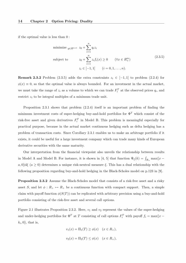
Remark 2.3.2 Problem (2.3.5) adds the extra constraints zi ∈ [−1, 1] to problem (2.2.4) for
φ(x) ≡ 0, so that the optimal value is always bounded. For an investment in the actual market,
we must take the range of zi as a volume to which we can trade F Ti at the observed prices qi, and
restrict zi to be integral multiples of a minimum trade unit.
Proposition 2.3.1 shows that problem (2.2.4) itself is an important problem of finding the
minimum investment costs of super-hedging buy-and-hold portfolios for ΦT which consist of the
risk-free asset and given derivatives F Ti in Model B. This problem is meaningful especially for
practical purpose, because in the actual market continuous hedging such as delta hedging has a
problem of transaction costs. Since Corollary 2.3.1 enables us to make an arbitrage portfolio if it
exists, it could be useful for a large investment company which can trade many kinds of European
derivative securities with the same maturity.
Our interpretation from the financial viewpoint also unveils the relationship between results
in Model A and Model B. For instance, it is shown in [4, 5] that function Ψξ(k) =∫R+
maxx −
a, 0dξ (a ≥ 0) determines a unique risk-neutral measure ξ. This has a dual relationship with the
following proposition regarding buy-and-hold hedging in the Black-Scholes model on p.123 in [9].
Proposition 2.3.2 Assume the Black-Scholes model that consists of a risk-free asset and a risky
asset S, and let φ : R+ 7→ R+ be a continuous function with compact support. Then, a simple
claim with payoff function φ(S(T )) can be replicated with arbitrary precision using a buy-and-hold
portfolio consisting of the risk-free asset and several call options.
Figure 2.1 illustrates Proposition 2.3.2. Here, v1 and v2 represent the values of the super-hedging
and under-hedging portfolios for ΦT at T consisting of call options F Ti with payoff fi = maxx −
ki, 0, that is,
v1(x) = Π1(T ) ≥ φ(x) (x ∈ R+),
v2(x) = Π2(T ) ≤ φ(x) (x ∈ R+),

2.4 Conclusion 15
y = v1(x)
y = v2(x)
y = φ(x)
k1 k2 k3 k4 k5
y
x = S(T )
Figure 2.1: Buy-and-hold hedging portfolios.
where Πj (j = 1, 2) are of the form
Πj(t) =n∑
i=1
zi,jFTi (t)
with certain constants zi,j (i = 1, 2, . . . , n, j = 1, 2). The relationship Π2(0) ≤ ΦT (0) ≤ Π1(0)
always holds, and Proposition 2.3.2 shows that Πj(0) can be made arbitrarily close to ΦT (0) by
letting n → +∞. Thus, the dual problem (2.2.4) could be more helpful to visualize the meaning
than problem (2.2.3). As a special case of problem (2.2.3), the problem of determining a price
range for a call option based on the observed prices of call options with other strikes has been fully
investigated in [6]. From the dual viewpoint we can state that it is a problem of finding an optimal
buy-and-hold hedging portfolio consisting of given call options.
2.4 Conclusion
This chapter has investigated the duality of the semi-infinite programming problem which arises
in the context of determining a derivative price range based only on the observed prices of other
derivatives and the no-arbitrage assumption (Model A). A contribution of this chapter is to give
an interpretation of the duality from the viewpoint of financial economics and reveal another

16 Chapter 2 Option Pricing: Duality
importance of studies in Model A. We have actually clarified that the dual of a problem of finding
the supremum on derivative prices with the observed prices of other derivatives in Model A is
equivalent to the problem of finding the minimum investment costs of buy-andhold super-hedging
portfolios for the derivative in the usual financial market model (Model B). This problem is useful
for investors because in the actual market rebalancing a hedging portfolio takes transaction costs.
The interpretation links some previous studies in Model A to the results for Model B in terms of
a buy-and-hold hedging portfolio.
Chapter 3
Option Pricing Based on Prices of
Other Derivatives: Risk-Neutral
Probabilities
3.1 Introduction
This chapter, as well as the previous chapter, investigates the option pricing based on the observed
prices of other derivatives without assuming any stochastic model for the dynamics of asset prices.
In particular, we investigate the problem of finding bounds on risk-neutral cumulative distribution
functions of the underlying asset price from the observed prices of call options, based only on
the no-arbitrage assumption. By considering this special case, we can analytically derive the
bounds on risk-neutral measures, which saves us from computing the numerous corresponding LPs
(linear programming problems) as discussed in [6]. We then compute the bounds from Nikkei-225
option data in Japan. To derive the risk-neutral measure implied from the real data is important,
because the risk-neutral measure plays a decisive role in pricing financial securities, and it represents
market’s view of risk. Actually, several studies such as [26] and [37] have investigated this problem
from other aspects.
This chapter is organized as follows. Section 3.2 explains the problem formulation and the
results obtained in [4]. Section 3.3 describes our main result, that is, the bounds on risk-neutral
measures in closed forms. Section 3.4 illustrates computational results obtained from Nikkei-225
option data in Japan.

18 Chapter 3 Option Pricing: Risk-Neutral Probabilities
3.2 Problem formulation
This section introduces the problem and describes some results obtained in [4], [5] and [6] for future
use.
We consider the problem of finding bounds on risk-neutral cumulative distribution functions of
the underlying asset price from the observed prices of European call options with exercise date T in
Model A which was introduced in Section 2.2. Throughout this chapter, we use the notations and
models introduced in Section 2.2. Then, the problem which we consider in this section becomes
problem (2.2.2) substituted φ(S(T )) = 1[0,a](S(T )) = P [S(T ) ∈ [0, a]] and fi(S(T )) = maxS(T )−
ki, 0, where 1[0,a](x) denotes the defining function of the set [0, a]. That is, for each a ≥ 0,
maximize P (∼P ) P [S(T ) ∈ [0, a]]
(or minimize)
subject to EP [maxS(T ) − ki, 0] = qi (i = 1, 2, . . . , n),
(3.2.1)
where P moves over the set of probability measures on (Ω,F) such that P is equivalent to the
observed probability measure P . Recall that P ∼ P in problem (3.2.1) denotes that P is a
probability measure equivalent to P . Here, for i = 1, 2, . . . , n, let qi denote the observed prices of
European call options with exercise date T and strikes ki at time 0. Without loss of generality, we
assume 0 ≤ k1 < k2 < · · · < kn in the rest of this chapter. Note that the demension of S(t), m,
is always equal to 1 in the setting of chapter. Note that the payoff of the call option is defined by
maxS(T )−ki, 0, because the holder of the call option receives S(T )−ki by exercising the option
on the exercise date T.
If we could derive the optimal values of problem (3.2.1) for all a ≥ 0, the upper and lower
bound functions can be obtained as functions of a ≥ 0. Note that the obtained bounds may not
be tight in the following sense: It is likely that no single risk-neutral probability measure P gives
the upper (or lower) bound function for all a ≥ 0, though for any fixed a ≥ 0 there exists a P that
attains the bound at a. To determine the bounds on risk-neutral cumulative distribution functions
is a fundamental question, because every European option on S(T ) can be priced from the implied
risk-neutral measure.
Since no particular dynamics of S(t) under P is assumed, the equivalence P ∼ P in problem
(3.2.1) does not add any restriction. Thus, by taking ξ as a distribution of S(T ) under P , we, like

3.2 Problem formulation 19
(2.2.3), rewrite problem (3.2.1) for each a ≥ 0,
maximize ξ∈Λ(R+) ξ([0, a])
(or minimize)
subject to∫
R+
maxx − ki, 0dξ = qi (i = 1, . . . , n),
(3.2.2)
Recall that Λ(R+) denotes the set of probability measures on the Borel space (R+,B(R+)) (see
Notaiton in Section 2.2). This problem is a concrete and solvable problem compared with the
abstract problem (3.2.1) on the probability space (Ω,F).
Problem (3.2.2) is a special case of the problems investigated in [6], because ξ([0, a]) is the same
as∫R+
1[0,a](x)dξ.
Although it involves the discontinuous payoff function 1[0,a](x), for a fixed a ≥ 0, problem
(3.2.2) can be reduced to an LP by using the same dual technique proposed in [6]. In this chapter,
however, we derive the infimum and the supremum of problem (3.2.2) as functions of a (≥ 0)
in closed forms. In other words, we can compute the upper and lower bounds without actually
solving the numerous LPs. From the dual viewpoint revealed in the previous chapter (see also
[67]), problem (3.2.2) is equivalent to finding the minimum costs necessary to super-hedge a binary
option with payoff 1[0,a](S(T )) with a buy-and-hold portfolio including the given call options in
Model B.
In most cases, not only the prices of the call options but also the underlying asset price S(0)
itself is observed. In this case, we have only to put k1 = 0 and take S(0) as q1, because the
underlying asset price is equal to the price of the call option with strike 0. If S(0) is observed
the results in this chapter can be also applied to European put options, because the prices of the
corresponding European call options can be derived from S(0) and the prices of put options via
the put-call parity (e.g., see p.123 in [9]), which is deduced only from the no-arbitrage assumption.
We note that the results in this chapter can also be applied to the modified problems, in
which S(T ) in problem (3.2.1) are replaced with the maximum asset price max0≤t≤T S(t) and the
average asset prices 1/T∫ T0 S(t)dt, by taking ξ as distributions of max0≤t≤T S(t) and 1/T
∫ T0 S(t)dt,
respectively.
Now, we describe the result derived in [4] before explaining our results. The following condition
will be assumed in the subsequent analysis:
Condition A The observed prices of European call options qi with strikes ki (where 0 ≤ k1 <

20 Chapter 3 Option Pricing: Risk-Neutral Probabilities
k2 < · · · < kn) satisfy
q1 ≥ q2 ≥ · · · ≥ qn ≥ 0,
α1 ≤ α2 ≤ · · · ≤ αn+1,
where αi = (qi − qi−1)/(ki − ki−1) (i = 2, . . . , n), α1 = −1 and αn+1 = 0. If there exists an
l (< n) such that ql = ql+1, then ql = ql+1 = · · · = qn = 0.
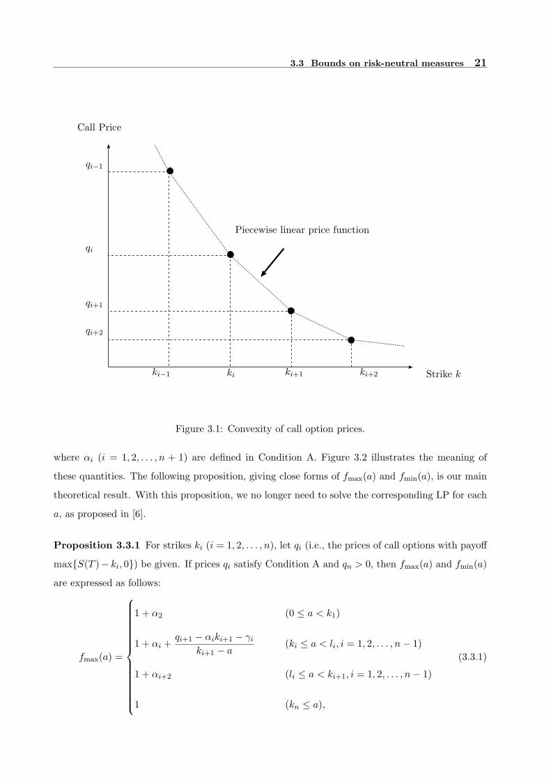
Condition A tells that the piecewise linear price function obtained by connecting points (ki, qi) (i =
1, 2, . . . , n) is convex and monotonically decreasing (see Figure 3.1).
For a ≥ 0, we define Ψξ(a) as the following function:
Ψξ(a) =∫
R+
maxx − a, 0dξ. (3.2.3)
This means the price of the call option with strike a under the assumption that the risk-neutral
measure is ξ. The following proposition proved in [4] shows that Condition A is a necessary and
sufficient condition for the existence of a risk-neutral measure ξ.
Proposition 3.2.1 At least one probability measure ξ on (R+,B(R+)) exists such that
Ψξ(ki) = qi (i = 1, . . . , n)
if and only if Condition A holds, where Ψξ is defined by (3.2.3).
Remark 3.2.1 Condition A is usually observed to hold on real data when the trade volume is
large. We will discuss this in Section 3.4 (see Figure 3.3).
3.3 Bounds on risk-neutral measures
This section derives the optimal values of problem (3.2.2) in closed forms, for both versions of
maximizing and minimizing the objective function. We then discuss potential applications of the
results.
Let fmax(a) and fmin(a) denote the optimal values of problem (3.2.2) to maximize and to
minimize, respectively. First, we introduce the following notations:
γi = qi − αiki (i = 1, 2, . . . , n),
γn+1 = qn,
li =γi − γi+2
αi+2 − αi(i = 1, 2, . . . , n − 1),
ln = − γn
αn,
3.3 Bounds on risk-neutral measures 21
Strike k
Call Price
Piecewise linear price function
ki−1 ki ki+1 ki+2
qi+2
qi+1
qi
qi−1
Figure 3.1: Convexity of call option prices.
where αi (i = 1, 2, . . . , n + 1) are defined in Condition A. Figure 3.2 illustrates the meaning of
these quantities. The following proposition, giving close forms of fmax(a) and fmin(a), is our main
theoretical result. With this proposition, we no longer need to solve the corresponding LP for each
a, as proposed in [6].
Proposition 3.3.1 For strikes ki (i = 1, 2, . . . , n), let qi (i.e., the prices of call options with payoff
maxS(T )− ki, 0) be given. If prices qi satisfy Condition A and qn > 0, then fmax(a) and fmin(a)
are expressed as follows:
fmax(a) =
1 + α2 (0 ≤ a < k1)
1 + αi +qi+1 − αiki+1 − γi
ki+1 − a(ki ≤ a < li, i = 1, 2, . . . , n − 1)
1 + αi+2 (li ≤ a < ki+1, i = 1, 2, . . . , n − 1)
1 (kn ≤ a),
(3.3.1)

22 Chapter 3 Option Pricing: Risk-Neutral Probabilities
!""#$%&'(
)*%&+(
Figure 3.2: Meanings of αi, γi, li.
fmin(a) =
0 (0 ≤ a < k1)
1 + αi+2 +γi+2 + αi+2ki − qi
a − ki(li ≤ a < ki+1, i = 1, 2, . . . , n − 1)
1 + αi (ki ≤ a < li, i = 1, . . . , n)
1 − qn
a − kn(ln ≤ a).
(3.3.2)
Proof Assume that Condition A and qn > 0 hold. Let Ψξ : R+ 7→ R+ be given by (3.2.3).
The following equality was proved in [4]:
Ψ′ξ(a+) = −ξ((a,∞])
= −1 + ξ([0, a]), (3.3.3)
where Ψ′ξ(a+) denotes the right derivative of Ψξ at a. By (3.3.3) and the definition of fmax and

3.3 Bounds on risk-neutral measures 23
fmin (i.e., optimal values of problem (3.2.2)) we have
fmax(a) = supξ∈Λ
ξ([0, a])
= 1 + supξ∈Λ
Ψ′ξ(a+). (3.3.4)
Here, Λ is the set of probability measures that satisfy the constraints of problem (3.2.2). Similarly,
we have
fmin(a) = 1 + infξ∈Λ
Ψ′ξ(a+). (3.3.5)
By Proposition 3.2.1, for a fixed a (≥ 0), there exists a probability measure ξ ∈ Λ satisfying
q = Ψξ(a) if and only if Condition A holds for the set of points consisting of (a, q) and (ki, qi) (i =
1, 2, . . . , n). Thus, we have
supξ∈Λ
Ψξ(a) =
α1a + γ1 (0 ≤ a < k1)
αi+1a + γi+1 (ki ≤ a < ki+1, i = 1, 2, . . . , n − 1)
qn (kn ≤ a)
(3.3.6)
and
infξ∈Λ
Ψξ(a) =
α2a + γ2 (k < k1)
αia + γi (ki ≤ a < li, i = 1, 2, . . . , n)
αi+2a + γi+2 (li ≤ a < ki+1, i = 1, 2, . . . , n − 1)
0 (ln ≤ a),
(3.3.7)
from the fact that the piecewise linear function connecting (a, q) and (ki, qi) (i = 1, 2, . . . , n) is
convex and decreasing. In Figure 3.2, the hatched regions between the upper dotted line and the
lower dotted lines illustrate the area of points (a, q) between (3.3.6) and (3.3.7). Extending this
results to all points a (≥ 0), we see that the price function Ψξ(a) must be a convex and decreasing
function contained in the hatched regions. Conversely, we can show, by modifying Proposition 3.2.1
as in [4], that there exists a ξ ∈ Λ such that Ψξ(a) = ψ(a) (a ≥ 0) for any convex and decreasing
function ψ(a) (a ≥ 0) in the hatched regions. Thus, by considering the right derivatives of all
convex and decreasing functions in the hatched regions in Figure 3.2, for ki ≤ a < li (i ≤ n − 1),

24 Chapter 3 Option Pricing: Risk-Neutral Probabilities
we have
supξ∈Λ
Ψ′ξ(a+) =
qi+1 − (αia + γi)ki+1 − a
(3.3.8)
= αi +qi+1 − αiki+1 − γi
ki+1 − a
infξ∈Λ
Ψ′ξ(a+) = αi. (3.3.9)
Here, the right-hand side of (3.3.8) is the gradient of the line connecting two points (ki+1, qi+1)
and (a, infξ∈Λ Ψξ(a)), and the right-hand side of (3.3.9) is the gradient of the lower dotted line for
ki ≤ k ≤ li in Figure 3.2. For li ≤ a < ki+1 (i ≤ n − 1), we have
supξ∈Λ
Ψ′ξ(a+) = αi+1 (3.3.10)
infξ∈Λ
Ψ′ξ(a+) =
αi+2a + γi+2 − qi
a − ki(3.3.11)
= αi+2 +γi+2 + αi+2ki − qi
a − ki,
where, the right-hand side of (3.3.10) is the gradient of the lower dotted line for li ≤ k ≤ ki+1
in Figure 3.2, and the right-hand side of (3.3.11) is the gradient of the line connecting two points
(ki, qi) and (a, infξ∈Λ Ψξ(a)). For the cases of a < k1 and kn ≤ a we can derive the supremum and
the infimum on the right derivatives in (3.3.4) and (3.3.5) by a similar geometric consideration.
The resulting functions are given as (3.3.1) and (3.3.2) in this proposition. 2
Remark 3.3.1 In the above proposition, we assumed qn > 0 for the practical reason that, in the
actual market, no call option can be traded at price 0. However similar results can be obtained
even if qn = 0 is allowed.
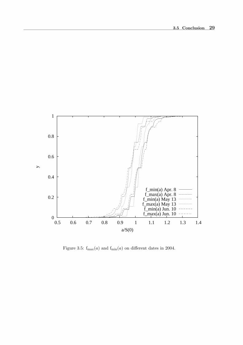
Remark 3.3.2 Figure 3.4 illustrates the functions fmax(a) and fmin(a) for some given data (as
will be discussed in Section 3.4).
3.4 Computational results
We compute the bounds of Proposition 3.3.1 from the data of Nikkei-225 options, which are most
popular in the option market of Japan. Then, the underlying asset price S(t) is the Nikkei-225
price at time t, and we took as qi the closing prices of the options with strike ki on the day 4
weeks before the exercise date (i.e., t = 0 on this day and t = T on the exercise date). We set the
risk-free rate as r = 0, as the maturity is only 4 weeks. For k1 = 0, q1 was taken as the closing

3.4 Computational results 25
price of Nikkei-225 on the day t = 0 (i.e., q1 = S(0)), because S(0) is identified as the price of the
call option with strike 0. We chose the data according to the following rules to improve the data
reliability:
(a) Use prices of all Nikkei-225 call and put options which have more than 500 trade volume.
(b) When both call and put options with the same strike and the same exercise date have more
than 500 trade volumes, choose the one which has a larger trade volume. Then, if put option
prices are chosen, determine the corresponding call option prices by applying the put-call
parity (i.e., the relation between prices of a call option and a put option, see p.123 in [9]).
We confirmed that the call option prices obtained by the above rules mostly satisfy Condition A.
An example is shown in Figure 3.3, which was computed from the data on March 11, 2004 (4 weeks
before the exercise date April 8, 2004). In Figure 3.3, there is a large blank area between k = 0
and 8500, because we used not only prices of the call options with strikes 8500, 9000, . . . , 13500 but
also the Nikkei-225 price S(0) = 11297 as the price of the call option with strike 0. For detailed
data, refer to Tables 3.1 and 3.2. Nikkei-225 options are usually traded with 14 strikes, which are
set at every 500 Japanese Yen around the present Nikkei-225 price.
0
2000
4000
6000
8000
10000
12000
0 2000 4000 6000 8000 10000 12000 14000
Pric
e
Strike
S(0) Price of Call Option
Figure 3.3: Prices of Nikkei-225 call options on March 11, 2004, with the exercise date of April 8,
2004.

26 Chapter 3 Option Pricing: Risk-Neutral Probabilities
Table 3.1: Data of Nikkei-225 options on March 11, 2004, with the exercise date April 8, 2004.
Strike Call Option Price Trade Volume Put Option Price Trade Volume Choose
7500 N/A 0 N/A 0 N/A
8000 N/A 0 N/A 0 N/A
8500 2780 30 N/A 0 N/A
9000 N/A 0 1 2840 Put
9500 N/A 0 4 3409 Put
10000 N/A 0 15 4128 Put
10500 810 32 55 3940 Put
11000 455 1188 180 866 Call
11500 200 1249 415 163 Call
12000 70 3044 775 94 Call
12500 20 1908 N/A 0 Call
13000 7 2328 N/A 0 Call
13500 2 1127 N/A 0 Call
Table 3.2: propositionices of call options on March 11, 2004, with the exercise date April 8, 2004.
Strike ki Price qi
0 11297
9000 2298
9500 1801
10000 1312
10500 852
11000 455
11500 200
12000 70
12500 20
13000 7
13500 2

3.4 Computational results 27
0
0.2
0.4
0.6
0.8
1
0.6 0.7 0.8 0.9 1 1.1 1.2 1.3 1.4
y
a/S(0)
y=f_min(a)y=f_max(a)
B.S.
Figure 3.4: fmax(a) and fmin(a) on April 8, 2004.
Then, we compute fmax(a) and fmin(a) by Proposition 3.3.1 from the data in Figure 3.3, and
illustrate them in Figure 3.4, where the scale of the x-axis is normalized by the present Nikkei-225
price S(0). For comparison, we also show the risk-neutral measure obtained from the Black-Scholes
model [10] with volatility σ = 0.2 (see B.S. in Figure 3.4); i.e., Φ((1/(σ√
T ))(log(a/S(0))+σ2T/2)),
where Φ(y) = (1/√
2π)∫ y−∞ e−x2/2dx denotes the standard normal cumulative distribution. Since
the risk-neutral measure in the Black-Scholes model does not exactly satisfy the constraints in
(3.2.2), the B.s. curve in Figure 3.4 slightly violates the boundaries of fmax(a) and fmin(a).
The results show that the difference between the upper and lower bounds is large in the region
close to the present Nikkei-225 price S(0) (i.e., a/S(0) ≈ 1) but it is small in the region far from
S(0). We also computed the bounds for 32 different exercise dates from January, 2002 to August,
2004, and confirmed that a similar trend always held for all exercise dates. For example, see Figure
3.5 showing the results for 3 different exercise dates in 2004.
In closing this section we suggest a few potential applications of our results. A first application
of Proposition 3.3.1 is of course to use the upper and lower bounds on ξ for the purpose of estimating
the price of European options.
Another use may be to utilize the above trend of the gap between the upper and lower bounds.
It tells that adding extra strikes in the region close to S(0) will reduce the difference between the

28 Chapter 3 Option Pricing: Risk-Neutral Probabilities
upper and lower bounds more efficiently than adding them in far regions. Smaller the difference,
the easier it becomes to hedge other European options with the same exercise date. As an extreme
case, let us assume that call options with all nonnegative strikes are actually traded. In this case,
the gap between the upper and lower bounds obtained from the observed prices becomes 0, and
therefore all European options with the same exercise date can be replicated by a buy-and-hold
portfolio consisting of several call options, meaning that the market is complete (for details see
the previous section [67]). Since one of the important roles of the option market is to change the
market closer to being complete, it is more meaningful to set the strikes, not equally spaced but less
spaced in the region near the present Nikkei-225 price S(0). In this way, we could use the bounds of
Proposition 3.3.1 to set the strikes with which the call options are traded. This suggestion will also
be supported by the observation that trade volume of the options became smaller for the strikes
set farther from the present Nikkei-225 price S(0) (e.g., see Table 3.1).
In general, the risk-neutral cumulative distribution function ξ tells us how investors view the
uncertain risk of S(T ). If the ξ implied by the computed bounds is similar to the cumulative
distribution function obtained from the historical data of the underlying asset price, we can expect
that investors in the market are risk-neutral. This kind of observation will help us when we make
investment in the market.
In analyzing Nikkei-225 data, we observed that the fmax and fmin computed by Proposition
3.3.1 showed different behaviors depending on whether S(T ) has actually become smaller or larger
than the S(0) of 4 weeks ago. This may suggest the possibility of using fmax and fmin to forecast
the future price of an asset, which would be one of our future topics.
3.5 Conclusion
This chapter investigated the problem of deriving the upper and lower bounds on risk-neutral
cumulative distribution functions of the underlying asset price from the observed prices of call
options, based only on the no-arbitrage assumption. The main contribution of this chapter is to
provide the bounds in closed forms, without solving the corresponding LPs. The bounds are easy
to compute. Based on the bounds computed from the real data of the Nikkei-225 options, we made
several observations and discussed possible applications, which could be used by investors. Finding
more applications of the computed bounds remains as an important and interesting issue.
3.5 Conclusion 29
0
0.2
0.4
0.6
0.8
1
0.5 0.6 0.7 0.8 0.9 1 1.1 1.2 1.3 1.4
y
a/S(0)
f_min(a) Apr. 8f_max(a) Apr. 8
f_min(a) May 13f_max(a) May 13f_min(a) Jun. 10f_max(a) Jun. 10
Figure 3.5: fmax(a) and fmin(a) on different dates in 2004.


Chapter 4
Real Options Involving Alternative
Investment Projects
4.1 Introduction
Real options approaches have become a useful tool for evaluating irreversible investment under
uncertainty such as R&D investment (see [22]). Although the early literature on real options (e.g.,
[20, 59]) treated the investment decision of a single firm, more recent studies provoked by [29] have
investigated the problem of several firms competing in the same market from a game theoretic
approach (see [13] for an overview). Grenadier [30] derived the equilibrium investment strategies
of the firms in the Cournot–Nash framework and Weeds [87] provided the asymmetric outcome
(called preemption equilibrium) in R&D competition between the two firms using the equilibrium
in a timing game studied in [27]. In [42, 83], a possibility of mistaken simultaneous investment
resulting from an absence of rent equalization that was assumed in [87] was investigated.
On the other hand, there are several studies on the decision of a single firm with an option to
choose both the type and the timing of the investment projects. In this literature, [21] was the first
study to pay attention to the problem and Decamps et al. [18] investigated the problem in more
detail. In [25], a similar model is applied to the problem of constructing small wind power units.
Despite such active studies on real options, to our knowledge few studies have tried to elucidate
how competition between two firms affects their investment decisions in the case where the firms
have the option to choose both the type and the timing of the projects. This chapter investigates the
above problem by extending the R&D model in [87] to a model where the firms can choose the target
of the research from two alternative technologies of different standards with the same uncertainty

32 Chapter 4 Real Options Involving Alternative Investment Projects
about the market demand1, where the technology standard is to be defined in some appropriate
sense. As in [87], technological uncertainty is taken into account, in addition to the product market
uncertainty. We assume that the time between project initiation and project discovery (henceforth
the research term) follows the Poisson distribution2 with its hazard rate determined by the standard
of the technology. This assumption is realistically intuitive since a higher-standard technology is
likely to require a longer research term and is expected to generate higher profits at its completion.
In the model, we show that the competition between the two firms affects not only the firms’
investment time, but also their choice of the technology targeted in the project. In fact, we observe
that the effect on the choice of the standard consists of two components. The presence of the
other firm straightforwardly changes the value of the technologies. We call this the direct effect
on the choice of the project type. In addition to the direct effect, the timing game caused by the
competition affects the firms’ choice of the targeted technology. This is due to the hastened timing
through the strategic interaction with the competitor; accordingly we call this the indirect effect,
distinguishedly from the direct effect.
We highlight two typical cases that are often observed in a market and, at the same time,
reveal interesting implications. The first case is that a firm that completes a technology first can
monopolize the profit flow regardless of the standard of the technology. De facto standardization
struggles such as VHS vs Betamax for video recorders are true for this case (henceforth called the
de facto standard case). In such cases, a firm can impose its technology as a de facto standard
by introducing it before its competitors. Once one technology becomes the de facto standard for
the market, the winner may well enjoy a monopolistic cash flow from the patent of the de facto
standard technology for a long term. It is then quite difficult for other firms to replace it with
other technologies even if those technologies are superior to the de facto standard one. Indeed, it
has been often observed in de facto standardization races that the existing technology drives out
a newer (superior) technology, which can be regarded as a sort of Gresham’s law3. In conclusion,
what is important in the de facto standard case is introducing the completed technology into the
market before the opponents.
1We assume that the two technologies are applied to homogeneous products.2Most studies, such as [16, 44, 55, 87], model technical innovation as a Poisson arrival; we also follow this conven-
tion.3Gresham’s law is the economic principle that in the circulation of money “bad money drives out good,” i.e., when
depreciated, mutilated, or debased coinage (or currency) is in concurrent circulation with money of high value in
terms of precious metals, the good money is withdrawn from circulation by hoarders.

4.1 Introduction 33
The other case is where a firm with higher-standard technology can deprive a firm with lower-
standard technology of the cash flow by completing the higher-standard technology. This case
applies to technologies of the innovative type (henceforth called the innovative case). As observed
in evolution from cassette-based Walkmans to CD- and MD-based Walkmans, and further to flash
memory- and hard drive-based digital audio players (e.g., iPod), the appearance of a newer tech-
nology drives out the existing technology. In such cases, a firm often attempts to develop a higher-
standard technology because it fears the invention of superior technologies by its competitors. As
a result, in the innovative case, a higher-standard technology tends to appear in a market.
The analysis in the two cases gives a good account of the characteristics mentioned above. In
the de facto standard case, the competition increases the incentive to develop the lower-standard
technology, which is easy to complete, while in the innovative case, the competition increases the
incentive to develop the higher-standard technology, which is difficult to complete. The increase
comes from both the direct and indirect effect of the completion. In particular, we show that
in the de facto standard case the competition is likely to lead the firms to invest in the lower-
standard technology, which is never chosen in the single firm situation. This result explains a real
problem caused by too bitter R&D competition. It is a possibility that the competition spoils the
higher-standard technology that consumers would prefer4, while the development hastened by the
competition increases consumers’ profits compared with that of the monopoly. That is, the result
accounts for both positive and negative sides of the R&D competition for consumers. Of course,
as described in [69], practical R&D management is often much more flexible and complex (e.g.,
growth and sequential options studied in [54, 51]) than the simple model in this chapter. However,
it is likely that the essence of the results remains unchanged in more practical setups.
In addition to the implications about the R&D competition given above, we also discuss our
theoretical contribution in relation to existing streams of the studies on real options with strategic
interactions. In fact, there are enormous number of papers that analyze strategic real options
models between two firms. While there is a stream of literature concentrating on incomplete and
asymmetric information5, our model is built on complete information. In literature under complete
information, Grenadier [29] proposed the basic model, and it has been extended to several directions
(e.g., involving the research term in [87], the exit decision in [63], the entry and exit decision in [28]).
Among those studies, a distinctive feature of our model is that the firms have the option to choose
4It is reasonable to suppose that consumers benefit from the invention of higher-standard technologies, though,
strictly speaking, we need to incorporate consumers’ value functions into the model.5See, for example, [31, 40, 50, 65, 66].

34 Chapter 4 Real Options Involving Alternative Investment Projects
the project type, which is properly defined in connection with the research term. Technically, we
combine the model by [87] with that of [18]. By doing so, we capture the simultaneous changes
of the investment timing and the choice of the project type due to the competition. In particular,
there is an interaction between the timing and project type choices (recall the indirect effect).
In terms of treating high and low standard technologies, this chapter is related to [43, 44]. Their
models give the technological innovation exogenously and assume that the firms can receive revenue
flows immediately after the investment using the available technology. Then, they show how the
possibility that a higher-standard technology will emerge in the future influences the investment
decision. In our model, on the other hand, the endogenous factor (i.e., the firm ’s choice of the
type and the timing of the investment projects) in addition to the exogenous one (i.e., randomness
in the research term) causes the technological innovation.
That is, the firm itself can trigger the technological innovation generating the patent value.
Thus, this chapter, unlike [43, 44], investigates the investment decision of R&D which will provoke
future technological innovation.
The chapter is organized as follows. After Section 4.2 derives the optimal investment timing
for the monopolist, Section 4.3 formulates the problem of the R&D competition between two firms.
Section 4.4 derives the equilibrium strategies in the two typical cases, namely, the de facto standard
case and the innovative case. Section 4.5 gives numerical examples, and finally Section 4.6 concludes
the chapter.
4.2 Single firm situation
Throughout Chapters 4–6, we assume all stochastic processes and random variables are defined on
the filtered probability space (Ω,F , P ;Ft). This chapter is based on the model in [87]. This section
considers the investment decision of the single firm without fear of preemption. The firm can set
up a research project for developing a new technology i (we denote technologies 1 and 2 for the
lower-standard and higher-standard technologies, respectively) by paying an indivisible investment
cost Ki. As in [87], for analytical advantage we assume that the firm has neither option to suspend
nor option to switch the projects, though practical R&D investment often allows more managerial
flexibility, such as to abandon, expand and switch (see [69]).
In developing technology i, from the time of the investment the invention takes place randomly
according to a Poisson distribution with constant hazard rate hi. The firm must pay the research
expense Ki per unit of time during the research term and can receive the profit flow DiY (t) from

4.2 Single firm situation 35
the discovery. Here, Y (t) represents a market demand of the technologies at time t and influence
cash flows which the technologies generate. It must be noted that the firm’s R&D investment
is affected by two different types of uncertainty (i.e., technological uncertainty and product mar-
ket uncertainty). For simplicity, Y (t) obeys the following geometric Brownian motion, which is
independent of the Poisson processes representing technological uncertainty.
dY (t) = µY (t)dt + σY (t)dB(t) (t > 0), Y (0) = y, (4.2.1)
where the voratility σ > 0 and the initial value y > 0 are given constants and B(t) denotes the
one-dimensional Ft standard Brownian motion. Quantities Ki, hi, Di and Ki are given constants
satisfying
0 ≤ K1 ≤ K2, 0 < h2 < h1, 0 < D1 < D2, 0 < K1 ≤ K2, (4.2.2)
so that technology 2 is more difficult to develop and generates a higher profit flow from its comple-
tion than technology 1.
Let us now comment upon the model. For analysis in later sections, we modified the original
setup by [87] at the two following points, but there are no essential difference. In [87], the completed
technology generates not a profit flow but a momentary profit as the value of the patent at its
completion, and there is no research expense during the research term (i.e, Ki = 0). In [44]
the Poisson process determining technological innovation is exogenous to the firms as in [32], but
we assume that a firm’s investment initiates the Poisson process determining the completion of
the technology. This is the main difference from the model studied in [44] that also treats two
technologies.
The firm that monitors the state of the market can set up development of either technologies 1
or 2 at the optimal timing maximizing the expected payoff under discount rate r(> µ). Then, the
firm’s problem is expressed as the following optimal stopping problem:
M(y) = supτ∈T
E
[maxi=1,2
E
[∫ ∞
τ+ti
e−rtDiY (t)dt − e−rτKi −∫ τ+ti
τe−rtKidt | Fτ
]], (4.2.3)
where T is a set of all Ft stopping times and ti denotes a random variable following the exponential
distribution with hazard rate hi. In problem (4.2.3), maxi=1,2 E[· | Fτ ] means that the firm can
choose the optimal technology at the investment time τ.

36 Chapter 4 Real Options Involving Alternative Investment Projects
By the calculation we obtain
E
[∫ ∞
τ+ti
e−rtDiY (t)dt − e−rτKi −∫ τ+ti
τe−rtKidt | Fτ
](4.2.4)
= e−rτEY (τ)
[∫ ∞
ti
e−rtDiY (t)dt − Ki −∫ ti
0e−rtKidt
](4.2.5)
= e−rτ
∫ ∞
0
(∫ ∞
se−rtDiE
Y (τ)[Y (t)]dt − Ki −∫ s
0e−rtKidt
)hie−hisds (4.2.6)
= e−rτ (ρi0Y (τ) − Ii), (4.2.7)
where we use the strong Markov property of Y (t) in (4.2.5) and independence between ti and Y (t)
in (4.2.6). Here, we need to explain the notation EY (τ)[·] in (4.2.5) and (4.2.6). For a real number
x, the notation Ex[·] denotes the expectation operator given that Y (0) = x, which can be changed
from the original initial value y. When the initial value is unchanged from the original value y, we
omit the superscript y, that is, E[·] = Ey[·]. The notation EY (τ)[·] represents the random variable
ψ(Y (τ)), where ψ(x) = Ex[·]. For example, Ex[Y (t)] is xeµt, and therefore EY (τ)[Y (t)] in (4.2.6)
becomes Y (τ)eµt. Thus, problem (4.2.3) can be reduced to
M(y) = supτ∈T
E[e−rτ maxi=1,2
(ρi0Y (τ) − Ii)], (4.2.8)
where ρi0 and Ii are defined by
ρi0 =Dihi
(r − µ)(r + hi − µ)(4.2.9)
Ii = Ki +Ki
r + hi. (4.2.10)
Here, ρi0Y (τ) represents the expected discounted value of the future profit generated by technology
i at the investment time τ, and Ii represents its total expected discounted cost at time τ.6 Eq. (4.2.2)
and (4.2.10) imply I1 < I2, but the inequality ρ10 < ρ20 does not necessarily hold depending upon
a trade-off between hi and Di. Note that (4.2.8) is essentially the same as the problem examined
in [18].
We make a brief explanation as to the difference between (4.2.8) and
M(y) = maxi=1,2
supτ∈T
E[e−rτ (ρi0Y (τ) − Ii)]
. (4.2.11)
(4.2.11) is a problem in which at time 0 the firm must decide which technology it develops. That
is, in problem (4.2.11), the firm cannot switch the technology even before the investment time τ
6Our setup is essentially the same as the setup by [87] that assumes Ki = 0, because we do not allow suspension
in the research term. That is, Ii defined by (4.2.10) can be regarded as a sunk investment cost. However, in this
chapter we consider Ki plus Ki in order to relate the cost Ii with the hazard rate hi.

4.2 Single firm situation 37
once the firm choose the technology at initial time. Since fewer cases of R&D investment applies to
the setting (4.2.11), we consider the setting (4.2.8) in which the firm can determine the technology
standard at the investment time τ . In addition, it holds that M(y) ≥ M(y) because the firm has
more managerial flexibility in problem (4.2.8) than in problem (4.2.11).
Let M(y) and τ∗M denote the value function and the optimal stopping time of problem (4.2.8),
respectively. The letter “M” means the case of monopoly. Note that τ∗M is expressed in a form
independent of the initial value y. As in most real options literature (e.g., [22]), we define
β10 =12− µ
σ2+
√(µ
σ2− 1
2
)2
+2r
σ2> 1, (4.2.12)
β20 =12− µ
σ2−
√(µ
σ2− 1
2
)2
+2r
σ2< 0. (4.2.13)
They are usual characteristic roots in an optimal stopping problem with discount rate r and state
process Y (t) following (4.2.1), and we can easily check β10 > 1 and β20 < 0.
Proposition 4.2.1 The value function M(y) and the optimal stopping time τ∗M of the monopolist
(4.2.8) are given as follows:
Case 1: 0 < ρ20/ρ10 ≤ 1
M(y) =
A0yβ10 (0 < y < y∗10)
ρ10y − I1 (y ≥ y∗10),(4.2.14)
τ∗M = inft ≥ 0 | Y (t) ≥ y∗10. (4.2.15)
Case 2: 1 < (ρ20/ρ10)β10/(β10−1) < I2/I1
M(y) =
A0yβ10 (0 < y < y∗10)
ρ10y − I1 (y∗10 ≤ y ≤ y∗20)
B0yβ10 + C0y
β20 (y∗20 < y < y∗30)
ρ20y − I2 (y ≥ y∗30),
(4.2.16)
τ∗M = inft ≥ 0 | Y (t) ∈ [y∗10, y
∗20] ∪ [y∗30, +∞). (4.2.17)
Case 3: (ρ20/ρ10)β10/(β10−1) ≥ I2/I1
M(y) =
B0yβ10 (0 < y < y∗30)
ρ20y − I2 (y ≥ y∗30),(4.2.18)
τ∗M = inft ≥ 0 | Y (t) ≥ y∗30. (4.2.19)
Here, constants A0, B0, C0 and thresholds y∗10, y∗20, y
∗30 are determined by imposing value matching
and smooth pasting conditions (see [22]). Note that I1 < I2 and β10 > 1.
38 Chapter 4 Real Options Involving Alternative Investment Projects
Proof In Case 2, (4.2.16) and (4.2.17) immediately follow from the discussion in [18]. In Case 1,
using relationships ρ10 ≥ ρ20, I1 < I2 and Y (t) > 0, we have
supτ∈T
E[e−rτ maxi=1,2
(ρi0Y (τ) − Ii)] = supτ∈T
E[e−rτ (ρ10Y (τ) − I1)],
which implies (4.2.14) and (4.2.15). In Case 3, by taking into consideration that the right-hand
side of (4.2.18) dominates ρ10y − I1, we can show (4.2.18) and (4.2.19) by a standard technique to
solve an optimal stopping problem (see [68]). 2
In Proposition 4.2.1, A0yβ10 , B0y
β10 and C0yβ20 correspond to the values of the option to invest
in technology 1 at the trigger y∗10, the option to invest in technology 2 at the trigger y∗30 and the
option to invest in technology 1 at the trigger y∗20, respectively. In Case 1, where the expected
discounted profit of technology 1 is higher than that of technology 2, the firm initiates development
of technology 1 at time (4.2.15) independently of the initial market demand y. In Case 3, where
technology 2 is much superior to technology 1, on the contrary, the firm invests in technology 2
at time (4.2.19) regardless of y. In Case 2, where both projects has similar values by the trade-off
between the profitability and the research term and cost, the firm’s optimal investment strategy
has three thresholds y∗10, y∗20 and y∗30, and therefore the project chosen by the firm depends on the
initial value y. Above all, if y ∈ (y∗20, y∗30), the firm defers not only investment, but also choice
among the two projects (i.e, whether the firm invests in technology 2 when the market demand
Y (t) increases to the upper trigger y∗30 or invests in technology 1 when Y (t) decreases to the lower
trigger y∗20). Hence, M(y) > M(y) holds only for y ∈ (y∗20, y∗30) in Case 2, while M(y) equals to
M(y) in other regions in Case 2 and other cases.
By letting volatility σ → +∞ with other parameters fixed, we have β10 → 1 by definition
(4.2.12) and therefore (ρ20/ρ10)β10/(β10−1) → +∞ if ρ10 < ρ20. As a result, with high product
market uncertainty, instead of Case 2, Case 3 holds and the firm chooses the higher-standard
technology 2 rather than the lower-standard technology 1, unless the expected discounted profit
generated by technology 1 exceeds that of technology 2. The similar result has also been mentioned
in [18].
4.3 Situation of two noncooperative firms
We turn now to a problem of two symmetric firms. This chapter considers a symmetric setting to
avoid unnecessary confusion, but the results in this chapter could remain true to some extent in
an asymmetric case. For a standard discussion of an asymmetric situation, see [42]. We assume

4.3 Situation of two noncooperative firms 39
that two Poisson processes modeling the two firms’ innovation are independent of each other, which
means that the progress of the research project by one of the firms does not affect that of its rival.
The scenarios of the cash flows into the firms can be classified into four cases. Figure 4.1 illustrates
the cash flows into the firm that has completed a technology first (denoted Firm 1) and the other
(denoted Firm 2).
!"#$%&' !"#$(&'$ )!#*
+,#-.*/!,0 +,#-.*/!,0
)*123$% )*123$%
)*123$% )*123$(
)*123$( )*123$!
Figure 4.1: (Firm 1’s cash flow, Firm 2’s cash flow).
In the period when a single firm has succeeded in the development of technology i, the firm
obtains the monopoly cash flow DiY (t). If both firms develop the same technology i, the one that
has completed first receives the profit flow DiY (t) resulting from the patent perpetually and the
other obtains nothing, according to the setup by [87]. Of course, the firm that has completed the
lower-standard technology 1 after the competitor’s completion of the higher-standard technology 2
obtains no cash flow. When the firm has completed technology 2 after the competitor’s completion
of technology 1, from the point technology 2 generates the profit flow ν2D2Y (t), and technology
1 generates ν1D1Y (t), where νi is a constant satisfying 0 ≤ ν1, ν2 ≤ 1. It is considered that the
technology’s share in the product market determines ν1 and ν2.
As usual (see the books [22, 42]), we solve the game between two firms backwards. We begin
by supposing that one of the firms has already invested, and find the optimal decision of the other.
In the remainder of this chapter, we call the one who has already invested leader and call the other
follower, though we consider two symmetrical firms. Thereafter, in the next section, we look at the
situation where neither firms has invested, and consider the decision of either as it contemplates
whether to go first, knowing that the other will react in the way just calculated as the follower’s

40 Chapter 4 Real Options Involving Alternative Investment Projects
optimal response. The main difference from the existing literature such as [22, 29, 42, 63, 87] is
that the follower’s optimal response depends on the technology i chosen by the leader. Let Fi(Y )
and τ∗Fi
denote the expected discounted payoff (at time t) and the investment time of the follower
responding optimally to the leader who has invested in technology i at time t satisfying Y (t) = Y.
We denote by Li(Y ) the expected discounted payoff (at time t) of the leader who has invested in
technology i at Y (t) = Y.
4.3.1 Case where the leader has invested in technology 2
This subsection derives F2(Y ), τ∗F2
and L2(Y ). Given that the leader has invested in technology 2
at Y (t) = Y, the follower solves the following optimal stopping problem:
F2(Y ) = ert supτ∈T ,τ≥t
E
[e−h2τ max
E
[1t1<s2
(∫ τ+s2
τ+t1
e−rsD1Y (s)ds
+∫ ∞
τ+s2
e−rsν1D1Y (s)ds
)− e−rτK1 −
∫ τ+t1
τe−rsK1ds | Fτ
],
E
[1t2<s2
∫ +∞
τ+t2
e−rsD2Y (s)ds − e−rτK2 −∫ τ+t2
τe−rsK2ds | Fτ
]| Y (t) = Y
],
(4.3.1)
where E[· | Y (t) = Y ] represents the expectation conditioned that Y (t) = Y . Recall ti represents a
random variable following the exponential distribution with hazard rate hi. The random variable
si is independent of ti and also follows the exponential distribution with hazard rate hi. Note that
the research term of the follower choosing technology i is expressed as ti in (4.3.1). The interval
between τ and the discovery time of the leader follows the exponential distribution with hazard rate
h2 (hence, it is expressed as s2 in (4.3.1)) under the condition that the leader has yet to complete
technology 2 at time τ . The reason is that the discovery occurs according to the Poisson process
which is Markovian. What has to be noticed is that the follower’s problem (4.3.2) is discounted by
e−h2τ differently from the single firm’s problem (4.2.3). This is because the leader’s completion of
technology 2 deprives the follower of the future option to invest. As in the single firm’s problem
(4.2.3), maxi=1,2 E[· | Fτ ] means that the follower chooses the better project at the investment time
τ. Furthermore, 1ti<s2 denotes a defining function and means that the follower’s payoff becomes
nothing if the leader completes technology 2 first. In order to derive F2(Y ) and τ∗F2
, we rewrite
problem (4.3.1) as the following problem with initial value Y (0) = Y , using the Markov property,
F2(Y ) = supτ∈T
EY
[e−h2τ max
EY
[1t1<s2
(∫ τ+s2
τ+t1
e−rsD1Y (s)ds
+∫ ∞
τ+s2
e−rsν1D1Y (s)ds
)− e−rτK1 −
∫ τ+t1
τe−rsK1ds | Fτ
],
EY
[1t2<s2
∫ +∞
τ+t2
e−rsD2Y (s)ds − e−rτK2 −∫ τ+t2
τe−rsK2ds | Fτ
]],
(4.3.2)

4.3 Situation of two noncooperative firms 41
where EY [·] means the (conditional) expectation operator given that the initial value Y (0) is Y
instead of y, as explained in page 36. Then, τ and s in problem (4.3.2), unlike those in (4.3.1),
represents how long it has passed since the leader’s investment time t. Strictly speaking, the
optimal stopping time in problem (4.3.2) is different from that in problem (4.3.1), τ∗F2
, since the
initial time in problem (4.3.2) corresponds to time t in problem (4.3.1). However, it is easy to
derive τ∗F2
from the solution in problem (4.3.2), and hence we hereafter identify problem (4.3.2)
with problem (4.3.1).
Via the similar calculation to (4.2.4)–(4.2.7) we can rewrite problem (4.3.2) as
F2(Y ) = supτ∈T
EY [e−(r+h2)τ maxi=1,2
(ρi2Y (τ) − Ii)], (4.3.3)
where ρij are defined by
ρ11 =D1h1
(r − µ)(r + 2h1 − µ), (4.3.4)
ρ12 =D1h1
(r + h1 + h2 − µ)(r + h2 − µ)
(1 +
ν1h2
r − µ
), (4.3.5)
ρ21 =D2h2
(r − µ)(r + h1 + h2 − µ)
(1 +
ν2h1
r + h2 − µ
), (4.3.6)
ρ22 =D2h2
(r − µ)(r + 2h2 − µ). (4.3.7)
Quantity ρijY (τ) represents the expected discounted value of the future cash flow of the firm that
invests in technology i at time τ when its opponent is on the way to development of technology j.
From the expression (4.3.3), we can show the following proposition.
Proposition 4.3.1 The follower’s payoff F2(Y ), investment time τ∗F2
and the leader’s payoff L2(Y )
are given as follows:
Case 1: 0 < ρ22/ρ12 ≤ 1
F2(Y ) =
A2Yβ12 (0 < Y < y∗12)
ρ12Y − I1 (Y ≥ y∗12),
τ∗F2
= infs ≥ t | Y (s) ≥ y∗12,
L2(Y ) =
ρ20Y − I2 − A2Yβ12 (0 < Y < y∗12)
ρ21Y − I2 (Y ≥ y∗12).
42 Chapter 4 Real Options Involving Alternative Investment Projects
Case 2: 1 < (ρ22/ρ12)β12/(β12−1) < I2/I1
F2(Y ) =
A2Yβ12 (0 < Y < y∗12)
ρ12Y − I1 (y∗12 ≤ Y ≤ y∗22)
B2Yβ12 + C2Y
β22 (y∗22 < Y < y∗32)
ρ22Y − I2 (Y ≥ y∗32),
τ∗F2
= infs ≥ t | Y (s) ∈ [y∗12, y∗22] ∪ [y∗32,+∞),
L2(Y ) =
ρ20Y − I2 − A2Yβ12 (0 < Y < y∗12)
ρ21Y − I2 (y∗12 ≤ Y ≤ y∗22)
ρ20Y − I2 − B2Yβ12 − C2Y
β22 (y∗22 < Y < y∗32)
ρ22Y − I2 (Y ≥ y∗32).
Case 3: (ρ22/ρ12)β12/(β12−1) ≥ I2/I1
F2(Y ) =
B2Yβ12 (0 < Y < y∗32)
ρ22Y − I2 (Y ≥ y∗32),
τ∗F2
= infs ≥ t | Y (s) ≥ y∗32,
L2(Y ) =
ρ20Y − I2 − B2Yβ12 (0 < Y < y∗32)
ρ22Y − I2 (Y ≥ y∗32).
Here, β12 and β22 denote (4.2.12) and (4.2.13) replaced r by r + h2, respectively. Here, r + h2
is the discount factor taking account of the possibility that the option is vanished with intensity
h2. After constants A2, B2, C2 and thresholds y∗12, y∗22, y
∗32 are determined by both value matching
and smooth pasting conditions in the follower’s value function F2(Y ), constants A2, B2 and C2 are
determined by the value matching condition alone in the leader’s payoff function L2(Y ). Note that
I1 < I2 and β12 > 1.
Proof Problem (4.3.3) coincides with problem (4.2.8) replaced r and ρi0 by r + h2 and ρi2,
respectively. Thus, we easily obtain the follower’s payoff F2(Y ) and investment time τ∗F2
in the
same way as Proposition 4.2.1. We next consider the leader’s payoff L2(Y ). In Case 1 and 3, we
readily have the same expression as that of [87] since the follower’s trigger is single. In Case 2,
we obtain the similar expression, though the calculation becomes more complicated because of the
three triggers. 2.
Constants A2, B2, C2 and thresholds y∗12, y∗22, y
∗32 in Proposition 4.3.1 correspond to constants
A0, B0, C0 and thresholds y∗10, y∗20, y
∗30 in Proposition 4.2.1, respectively. Let us explain the leader’s
payoff briefly. Constants A2, B2 and C2 value the possibility that Y rises above y∗12 prior to the

4.3 Situation of two noncooperative firms 43
leader’s completion, the possibility that Y rises above y∗32 prior to the leader’s completion, and
the possibility that Y falls bellow y∗22 prior to the leader’s completion, respectively. Since these
situations cause the follower’s investment, the leader’s payoff is reduced from the monopoly profit
ρ20Y − I2 (see Y ∈ (0, y∗12) in Case 1, Y ∈ (0, y∗12)∪ (y∗22, y∗32) in Case 2, and Y ∈ (0, y∗32) in Case 3).
4.3.2 Case where the leader has invested in technology 1
We now consider F1(Y ), τ∗F1
and L1(Y ). In the previous subsection, i.e., in the case where the
leader has chosen technology 2, the follower’s opportunity to invest is completely lost at the leader’s
completion of technology 2. However, in the case where the leader has invested in technology 1,
there remains the inactive follower’s option after the leader’s invention of technology 1. That is,
the follower can invest in technology 2 even after the leader’s discovery if the follower has not
invested in any technology yet. Due to this option value, we need more complicated discussion in
this subsection.
Let f1(Y ) and τ∗f1
be the expected discounted payoff and the optimal stopping time of the
follower responding optimally to the leader who has already succeeded in development of technology
1 at Y (t) = Y. In other words, f1(Y ) represents the remaining option value to invest in technology
2 after the leader’s completion of technology 1. We need to derive f1(Y ) and τ∗f1
before analyzing
F1(Y ) and τ∗F1
. Given that the leader has already completed technology 1 at Y (t) = Y, the follower’s
problem becomes
f1(Y ) = supτ∈T
EY
[∫ ∞
τ+t2
e−rtν2D2Y (t)dt − e−rτK2 −∫ τ+t2
τe−rtK2dt
], (4.3.8)
which is equal to a problem of a firm that can develop only technology 2. In this subsection, we
omit a description of a problem which corresponds to (4.3.1), and describe only a problem (which
corresponds to (4.3.1)) with initial value Y (0) = Y . In the same way as calculation (4.2.4)–(4.2.7),
we can rewrite problem (4.3.8) as
f1(Y ) = supτ∈T
EY [e−rτ (ν2ρ20Y (t) − I2)]. (4.3.9)
It is easy to obtain the value function f1(Y ) and the optimal stopping time τ∗f1
of the follower. If
ν2 > 0, then
f1(Y ) =
B′Y β10 (0 < Y < y′)
ν2ρ20Y − I2 (Y ≥ y′),(4.3.10)
τ∗f1
= infs ≥ t | Y (s) ≥ y′, (4.3.11)

44 Chapter 4 Real Options Involving Alternative Investment Projects
where B′ and y′ are constants determined by the value matching and smooth pasting conditions
(we omit the explicit solutions to avoid cluttering). If ν2 = 0, we have f1(Y ) = 0 and τ∗f1
= +∞.
Assuming that the leader has begun developing technology 1 at Y (t) = Y, the follower’s problem
is expressed as follows:
F1(Y ) = supτ∈T
EY
[e−h1τ max
EY
[1t1<s1
∫ +∞
τ+t1
e−rsD1Y (s)ds − e−rτK1 −∫ τ+t1
τe−rsK1ds | Fτ
],
EY
[1t2<s1
∫ +∞
τ+t2
e−rsD2Y (s)ds + 1t2≥s1
∫ +∞
τ+t2
e−rsν2D2Y (s)ds − e−rτK2
−∫ τ+t2
τe−rsK2ds | Fτ
]+ 1τ≥s′1e
−rs′1 f1(Y (s′1))]
,
(4.3.12)
where s′1 represents another random variable following the exponential distribution with hazard
rate h2. In (4.3.12), the interval between the leader’s investment time t and completion time is
expressed as s′1. By the Markov property, the interval between t and the completion time of the
non-conditional leader has the same distribution as the interval between τ and the completion
time of the leader who is conditioned to be yet to complete technology 1 at τ . Compared with
the follower’s problem (4.3.2) in the previous subsection, problem (4.3.12) has the additional term
EY [1τ≥s′1e−rs′1 f1(Y (s′1))]. This term corresponds to the remaining option value of the inactive
follower. As in (4.2.4)–(4.2.7), problem (4.3.12) can be reduced to
F1(Y ) = supτ∈T
EY [e−(r+h1)τ maxi=1,2
(ρi1Y (τ) − Ii) + 1τ≥s′1e−rs′1 f1(Y (s′1))], (4.3.13)
where ρ11 and ρ21 are defined by (4.3.4) and (4.3.6), respectively. Generally, problem (4.3.13),
unlike (4.3.3), is difficult to solve analytically because of the additional term. In the next section,
we overcome the difficulty by focusing on two typical cases, namely, the de fact standard case,
where (ν1, ν2) = (1, 0), and the innovative case, where (ν1, ν2) = (0, 1).
4.4 Analysis in two typical cases
This section examines the firms’ behaviour in the de fact standard case, where (ν1, ν2) = (1, 0), and
the innovative case, where (ν1, ν2) = (0, 1). In the real world both ν1 > 0 and ν2 > 0 are usually
hold and the two cases are extreme. However, such a real case approximates to one of the two cases
or has an intermediate property, depending on the relationship between ν1 and ν2, and therefore
analysis in the two cases helps us to understand the essence of the problem. In order to exclude a

4.4 Analysis in two typical cases 45
situation where both firms mistakenly invest simultaneously7, we assume that the initial value y is
small enough, that is,
Assumption A
maxi=1,2
(ρi0y − Ii) < 0,
as in [87] when we discuss the firms’ equilibrium strategies. Assumption A is likely to hold in the
context of R&D. A firm tends to delay its investment decision of R&D (rarely invest immediately),
because the R&D investment decision is carefully made taking account of the distant future.
We moreover restrict our attention to the case where the firm always chooses the higher-standard
technology 2 in the single firm situation, for the purpose of contrasting the competitive situation
with the single firm situation. To put it more concretely, we assume
Assumption B (ρ20
ρ10
) β10β10−1
≥ I2
I1,
so that Case 3 follows in Proposition 4.2.1.
In the first place, we analytically derive the follower’s payoff F1(Y ) and the leader’s payoff
L1(Y ) in both de fact standard and innovative cases. Note that the results on F2(Y ) and L2(Y )
in Proposition 4.3.1 hold true by substituting (ν1, ν2) = (1, 0) and (ν1, ν2) = (0, 1) into (4.3.5) and
(4.3.6). Then,we compare the leader’s payoff L(Y ) with the follower’s payoff F (Y ), where L(Y )
and F (Y ) are defined by
L(Y ) = maxi=1,2
Li(Y ),
F (Y ) =
F1(Y ) (L1(Y ) > L2(Y ))
F2(Y ) (L1(Y ) ≤ L2(Y )).
By the comparison, we see the situation where both firms try to preempt each other.
4.4.1 De facto standard case
Since ν2 = 0 holds in this case, the follower’s option value f1(Y (s′1)) vanishes just like in Subsection
3.2. Thus, we can solve the follower’s problem (4.3.13) in the same way as problem (4.3.3). Indeed,
F1(Y ) and τ∗F1
agree with F2(Y ) and τ∗F2
replaced ρi2, βi2 with ρi1, βi1, respectively in Proposition7We must distinguish between mistaken simultaneous investment and joint investment which is examined in
Subsection 4.3. For the details of the stopping time game, see Appendix A.

46 Chapter 4 Real Options Involving Alternative Investment Projects
4.3.1, where β11 (> 1) and β21 (< 0) denote (4.2.12) and (4.2.13) replaced discount rate r with
r + h1, respectively. Recall that ρ11 and ρ21 were defined by (4.3.4) and (4.3.6). In this case, we
denote three thresholds corresponding to y∗12, y∗22 and y∗32 in Proposition 4.3.1 by y∗11, y
∗21 and y∗31,
respectively. Then, the payoff L1(Y ) of the leader who has invested in technology 1 at Y (t) = Y
coincides with L2(Y ) replaced ρ2i, I2, βi2 and y∗i2 by ρ1i, I1, βi1 and y∗i1, respectively in Proposition
4.3.1.
Let us compare the follower’s decision in the de facto standard case with the single firm’s
decision derived in Section 4.2. Using
ρ20
ρ10=
D2h2(r + h1 − µ)D1h1(r + h2 − µ)
>D2h2(r + h1 + h2 − µ)D1h1(r + h2 + h2 − µ)
=ρ22
ρ12
>D2h2(r + h1 + h1 − µ)D1h1(r + h2 + h1 − µ)
=ρ21
ρ11,
which result from r − µ > 0 and h1 > h2 > 0, we have
ρ21
ρ11<
ρ22
ρ12<
ρ20
ρ10. (4.4.1)
Eq. (4.4.1) states that the relative expected profit of technology 2 to technology 1 is smaller than
that of the single firm case. Using 1 < β10 < β12 < β11, we also obtain
1 <β11
β11 − 1<
β12
β12 − 1<
β10
β10 − 1. (4.4.2)
Eqs. (4.4.1) and (4.4.2) suggest a possibility that (ρ2i/ρ1i)β1i/(β1i−1) is smaller than I2/I1 and 1 even
under Assumption B, and then the follower’s optimal choice could be technology 1. In consequence,
the presence of the leader increases the follower’s incentive to choose the lower-standard technology
1, which is easy to complete, compared with in the single firm situation (the direct effect).
From ρi1 < ρi2, r + h2 < r + h1, problem formulations (4.3.3) and (4.3.13) (note that f1 = 0 in
the de facto standard case), it follows that
F1(Y ) < F2(Y ) (Y > 0).
That is, from the follower’s viewpoint, the case where the leader has chosen technology 2 is prefer-
able to the case where the leader has chosen technology 1. This is due to that the leader who has
invested in technology 1 is more likely to preempt the follower because of its short research term.
Finally, we take a look at the situation where neither firm has invested. Let us see that there
exists a possibility that technology 1 can be developed owing to the competition even if technology

4.4 Analysis in two typical cases 47
2 generates much more profit than technology 1 at its completion. Although, as has been pointed
out, (ρ2i/ρ1i)β1i/(β1i−1) could be smaller than I2/I1 and 1 under Assumption B, we now consider
the case where (ρ2i
ρ1i
) β1iβ1i−1
≥ I2
I1(4.4.3)
holds, which means that a cash flow resulting from technology 2 is expected to be much greater
than that of technology 1.
Since the initial value Y (0) = y is small enough (Assumption A), in the single firm situation
the firm invests in technology 2 (Assumption B) as soon as the market demand Y (t) rises to the
level y∗30 (Figure 4.2). Development of technology 1 is meaningless because the firm without fear
of preemption can defer the investment sufficiently. However, the firm with the fear of preemption
by its rival will try to obtain the leader’s payoff by investing a slight bit earlier than its rival when
the leader’s payoff L(Y ) is larger than the follower’s payoff F (Y ). Repeating this process causes
the investment trigger to fall to the point where L(Y ) is equal to F (Y ) (yP in Figure 4.3). At
the point the firms are indifferent between the two roles, and then one of the firms invests at
time inft ≥ 0 | Y (t) ≥ yP as leader, while the other invests at time τ∗Fi
(if there remains the
option to invest) as follower. This phenomenon is rent equalization explained in [27, 87]. This
asymmetric outcome where one of the firms becomes a leader and the other becomes a follower is
called preemption equilibrium. For further details of the stopping time game and the equilibrium,
see Appendix A. If the fear of preemption hastens the investment time sufficiently (e.g., threshold
yP becomes smaller than y in Figure 4.2), then threshold yP becomes the intersection of L1(Y ) and
F1(Y ) rather than the intersection of L2(Y ) and F2(Y ) (Figure 4.3). It suggests a possibility that
in the preemption equilibrium the leader invests in technology 1 (the indirect effect). Needless to
say, the leader is more likely to choose technology 1 if (4.4.3) is not satisfied. The above discussion
gives a good account of the phenomenon observed frequently in de facto standard wars.
4.4.2 Innovative case
This subsection examines the innovative case, where (ν1, ν2) = (0, 1) is satisfied. We now consider
the follower’s optimal response assuming that the leader has invested in technology 1 at Y (t) = Y.
Let F1(Y ) denote the payoff (strictly speaking, the expected discounted payoff at time t) of the
follower who initiate developing technology 2 at time τ∗f1
defined by (4.3.11). We can show that
in the innovative case the follower’s best response τ∗F1
coincides with τ∗f1
and also show F1(Y ) =
f1(Y ) = F1(Y ) = M(Y ) as follows.
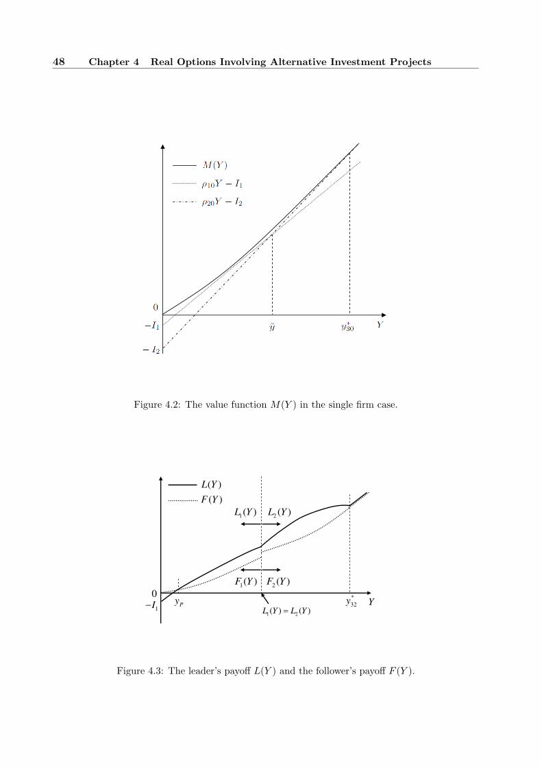
48 Chapter 4 Real Options Involving Alternative Investment Projects
Figure 4.2: The value function M(Y ) in the single firm case.
1I
( )L Y
( )F Y
1( )L Y
2( )L Y
1( )F Y
2( )F Y
Py
0 *
32y Y
1 2( ) ( )L Y L Y
Figure 4.3: The leader’s payoff L(Y ) and the follower’s payoff F (Y ).

4.4 Analysis in two typical cases 49
By ν2 = 1, the payoff of the follower who invests in technology 2 at time s (≥ t) is ρ20Y (s)− I2,
whether the leader has completed technology 1 or not. Then we have F1(Y ) = f1(Y ). Under
Assumption B the single firm’s value function M(Y ) is expressed as that of Case 3 in Proposition
4.2.1. Using ν2 = 1, we have
M(Y ) = f1(Y ) = F1(Y ). (4.4.4)
On the other hand, by definition of the follower’s problem (4.3.13), it can readily be seen that the
relationship
F1(Y ) ≤ M(Y ) (4.4.5)
holds between F1(Y ) and M(Y ). Note that the follower’s option value to invest in technology 2 is the
same as that of the single firm case. In contrast, the follower’s option value to invest in technology
1 is lower than that of the single firm case. The reason is that the follower’s option value to invest
in technology 1 vanishes completely at the leader’s invention of technology 1. Eqs. (4.4.4) and
(4.4.5) suggest F1(Y ) ≤ F1(Y ). Thus, we have F1(Y ) = F1(Y ), taking account of F1(Y ) ≥ F1(Y )
resulting from the optimality of F1(Y ). Consequently, the follower’s optimal response τ∗F1
coincides
with τ∗f1
and F1(Y ) = f1(Y ) = F1(Y ) = M(Y ) holds. We should notice that the follower behaves
as if there were no leader.
Using the follower’s investment time τ∗F2
= τ∗f1
derived above (note that y′ = y∗30 in (4.3.11) by
ν2 = 1), we have the leader’s payoff L1(Y ) as L2(Y ) replaced ρ2i, I2, β12 and y∗32 by ρ1i, I1, β11 and
y∗30, respectively in Case 3 in Proposition 4.3.1.
Next, we compare the follower’s decision in the innovative case with the single firm’s decision.
Using
ρ20
ρ10=
ρ22
ρ12× r + h1 − µ
r + h1 + h2 − µ× (r − µ)(r + 2h2 − µ)
(r + h2 − µ)2
<ρ22
ρ12,
ρ21 = ρ20 and ρ11 < ρ10, we have
1 <ρ20
ρ10<
ρ2i
ρ1i(i = 1, 2). (4.4.6)
Eq. (4.4.6) means that the relative expected profit of technology 2 to technology 1 is greater than
that of the single firm case, contrary to (4.4.1) in the de facto standard case. Since (4.4.2) remains
true, the relationship between (ρ22/ρ12)β12/(β12−1) and I2/I1 depends on the parameters even under
Assumption B. This suggests a slight possibility that the follower chooses technology 1 in the case
where the leader has chosen technology 2, while as we showed in the beginning of this subsection

50 Chapter 4 Real Options Involving Alternative Investment Projects
the follower’s best response to the leader who has invested in technology 1 is choosing technology
2 regardless of Y . However, in most cases the effect of (4.4.6) dominates the effect of (4.4.2), that
is,
I2
I1<
(ρ20
ρ10
) β10β10−1
<
(ρ22
ρ12
) β12β12−1
hold. To sum up, the presence of the leader, unlike in the de facto standard case, tends to decreases
the incentive of the lower-standard technology 1, which is easy to complete (the direct effect).
By definition of the follower’s problem (4.3.3) we can immediately show
F2(Y ) < M(Y ) = F1(Y ) (Y > 0).
In other words, contrary to the de facto standard case, the follower prefers the leader developing
technology 1 to the leader developing technology 2. This is because the follower can deprive the
leader who has chosen technology 1 of the profit by completing technology 2.
Finally, let us examine the situation where neither firm has taken action. We obtain the
following proposition with respect to the preemption equilibrium.
Proposition 4.4.1 The inequality
L1(Y ) < F1(Y ) (Y > 0) (4.4.7)
holds, and therefore in the preemption equilibrium the leader always chooses technology 2. Fur-
thermore, if (ρ22
ρ12
) β12β12−1
>I2
I1(4.4.8)
(Eq. (4.4.8) is satisfied for reasonable parameter values as mentioned earlier), then in the preemp-
tion equilibrium the follower, also, always chooses technology 2.
Proof The leader’s payoff L1(Y ) is equal to
L1(Y ) =
ρ10Y − I1 − B1Yβ12 (0 < Y < y∗30)
ρ12Y − I1 (Y ≥ y∗30),
where the constant B1 > 0 is determined by the value matching condition at the trigger y∗30. Using
ρ10 > ρ12 and B1 > 0, we have
L1(Y ) < ρ10Y − I1 ≤ M(Y ) = F1(Y ) (Y > 0),
which implies that there is no incentive to invest in technology 1 earlier than the competitor.
Therefore, there arises no preemption equilibrium where the leader invests in technology 1. Next,
4.4 Analysis in two typical cases 51
we assume (4.4.8). In this case, the follower’s decision corresponds to that of Case 3 in Proposition
4.2.1. In consequence, in the preemption equilibrium, the follower, also, always chooses technology
2. 2
Table 4.1 summarizes the comparison results between the de facto standard and innovative
cases.
4.4.3 Case of joint investment
The joint investment equilibria, which are, unlike the preemption equilibria, symmetric outcomes,
may also occur even if the two firms are noncooperative. The results on the joint investment
equilibria in our setup is similar to that in [87] and therefore they are briefly described below.
Assuming that the two firms are constrained to invest in the same technology at the same
timing, the firm’s problem can be reduced to
J(y) = supτ∈T
E[e−rτ maxi=1,2
(ρiiY (τ) − Ii)], (4.4.9)
in the same procedure as (4.2.4)–(4.2.7). Recall that ρ11 and ρ22 were defined by (4.3.4) and (4.3.7),
respectively. It is worth noting that the expression (4.4.9) does not depend on whether the de facto
standard case or the innovative case. Using
ρ20
ρ10=
D2h2(r + h1 − µ)D1h1(r + h2 − µ)
<D2h2(r + 2h1 − µ)D1h1(r + 2h2 − µ)
=ρ22
ρ11
and Assumption B, we have
I2
I1<
(ρ20
ρ10
) β10β10−1
<
(ρ22
ρ11
) β10β10−1
.
Thus, the value function (denoted by J(y)) and the optimal stopping time (denoted by τ∗J ) of
problem (4.4.9) coincide with M(Y ) and τ∗0 replaced ρ20 with ρ22 in Case 3 in Proposition 4.2.1,
that is, the two firms set up the development of technology 2 at the same time
τ∗J = inft ≥ 0 | Y (t) ≥ y∗33, (4.4.10)
where y33 denotes the joint investment trigger corresponding to y30 in Proposition 4.2.1. The letter
“J” refers to the case of joint investment. As in the single firm case, in joint investment both firms
always choose technology 2.
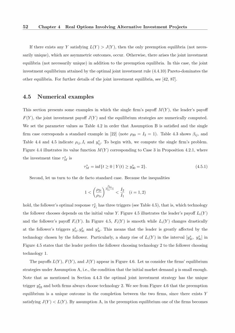
52 Chapter 4 Real Options Involving Alternative Investment Projects
If there exists any Y satisfying L(Y ) > J(Y ), then the only preemption equilibria (not neces-
sarily unique), which are asymmetric outcomes, occur. Otherwise, there arises the joint investment
equilibria (not necessarily unique) in addition to the preemption equilibria. In this case, the joint
investment equilibrium attained by the optimal joint investment rule (4.4.10) Pareto-dominates the
other equilibria. For further details of the joint investment equilibria, see [42, 87].
4.5 Numerical examples
This section presents some examples in which the single firm’s payoff M(Y ), the leader’s payoff
F (Y ), the joint investment payoff J(Y ) and the equilibrium strategies are numerically computed.
We set the parameter values as Table 4.2 in order that Assumption B is satisfied and the single
firm case corresponds a standard example in [22] (note ρ20 = I2 = 1). Table 4.3 shows βij , and
Table 4.4 and 4.5 indicate ρij , Ii and y∗ij . To begin with, we compute the single firm’s problem.
Figure 4.4 illustrates its value function M(Y ) corresponding to Case 3 in Proposition 4.2.1, where
the investment time τ∗M is
τ∗M = inft ≥ 0 | Y (t) ≥ y∗30 = 2. (4.5.1)
Second, let us turn to the de facto standard case. Because the inequalities
1 <
(ρ2i
ρ1i
) β1iβ1i−1
<I2
I1(i = 1, 2)
hold, the follower’s optimal response τ∗Fi
has three triggers (see Table 4.5), that is, which technology
the follower chooses depends on the initial value Y. Figure 4.5 illustrates the leader’s payoff Li(Y )
and the follower’s payoff Fi(Y ). In Figure 4.5, Fi(Y ) is smooth while Li(Y ) changes drastically
at the follower’s triggers y∗1i, y∗2i and y∗3i. This means that the leader is greatly affected by the
technology chosen by the follower. Particularly, a sharp rise of Li(Y ) in the interval [y∗2i, y∗3i] in
Figure 4.5 states that the leader prefers the follower choosing technology 2 to the follower choosing
technology 1.
The payoffs L(Y ), F (Y ), and J(Y ) appear in Figure 4.6. Let us consider the firms’ equilibrium
strategies under Assumption A, i.e., the condition that the initial market demand y is small enough.
Note that as mentioned in Section 4.4.3 the optimal joint investment strategy has the unique
trigger y∗33 and both firms always choose technology 2. We see from Figure 4.6 that the preemption
equilibrium is a unique outcome in the completion between the two firms, since there exists Y
satisfying J(Y ) < L(Y ). By assumption A, in the preemption equilibrium one of the firms becomes

4.5 Numerical examples 53
Table 4.1: Comparison between the de facto standard and innovative cases.
De facto standard Innovative
Relative expected profit ρ2i/ρ1i < ρ20/ρ10 ρ2i/ρ1i > ρ20/ρ10
Follower’s value function F1(Y ) < F2(Y ) F1(Y ) > F2(Y )
Preemption equilibrium Both firms: likely to choose
Tech. 1
Leader: Tech. 2, Follower:
Tech. 2 (in most cases)
Table 4.2: Parameter setting.
r µ σ D1 D2 h1 h2 K1 K2 K1 K2
0.04 0 0.2 0.025 0.05 0.32 0.16 0 0 0.18 0.2
Table 4.3: βij .
β10 β20 β11 β21 β12 β22
2 1 4.77 −3.77 3.7 −2.7
Table 4.4: Values common to both cases.
ρ10 ρ20 ρ11 ρ22 I1 I2 y∗30 y∗33
0.56 1 0.29 0.56 0.5 1 2 3.6
Table 4.5: Values dependent on the cases.
ρ12 ρ21 y∗11 y∗21 y∗31 y∗12 y∗22 y∗32
De facto standard 0.38 0.38 2.15 5.46 5.59 1.78 2.81 3.04
Innovative 0.08 1 N/A N/A 2 N/A N/A 2.47
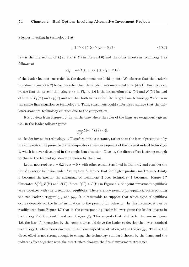
54 Chapter 4 Real Options Involving Alternative Investment Projects
a leader investing in technology 1 at
inft ≥ 0 | Y (t) ≥ yP = 0.93 (4.5.2)
(yP is the intersection of L(Y ) and F (Y ) in Figure 4.6) and the other invests in technology 1 as
follower at
τ∗F1
= inft ≥ 0 | Y (t) ≥ y∗11 = 2.15
if the leader has not succeeded in the development until this point. We observe that the leader’s
investment time (4.5.2) becomes earlier than the single firm’s investment time (4.5.1). Furthermore,
we see that the preemption trigger yP in Figure 4.6 is the intersection of L1(Y ) and F1(Y ) instead
of that of L2(Y ) and F2(Y ) and see that both firms switch the target from technology 2 chosen in
the single firm situation to technology 1. Thus, consumers could suffer disadvantage that the only
lower-standard technology emerges due to the competition.
It is obvious from Figure 4.6 that in the case where the roles of the firms are exogenously given,
i.e., in the leader-follower game
supτ∈T
E[e−rτL(Y (τ))],
the leader invests in technology 1. Therefore, in this instance, rather than the fear of preemption by
the competitor, the presence of the competitor causes development of the lower-standard technology
1, which is never developed in the single firm situation. That is, the direct effect is strong enough
to change the technology standard chosen by the firms.
Let us now replace σ = 0.2 by σ = 0.8 with other parameters fixed in Table 4.2 and consider the
firms’ strategic behavior under Assumption A. Notice that the higher product market uncertainty
σ becomes the greater the advantage of technology 2 over technology 1 becomes. Figure 4.7
illustrates L(Y ), F (Y ) and J(Y ). Since J(Y ) > L(Y ) in Figure 4.7, the joint investment equilibria
arise together with the preemption equilibria. There are two preemption equilibria corresponding
the two leader’s triggers yP1 and yP2 . It is reasonable to suppose that which type of equilibria
occurs depends on the firms’ inclination to the preemption behavior. In this instance, it can be
readily seen from Figure 4.7 that in the corresponding leader-follower game the leader invests in
technology 2 at the joint investment trigger y∗33. This suggests that relative to the case in Figure
4.6, the fear of preemption by the competitor could drive the leader to develop the lower-standard
technology 1, which never emerges in the noncompetitive situation, at the trigger yP1 . That is, the
direct effect is not strong enough to change the technology standard chosen by the firms, and the
indirect effect together with the direct effect changes the firms’ investment strategies.

4.6 Conclusion 55
Finally, we examine the innovative case. It can be deduced from the inequality(ρ22
ρ12
) β12β12−1
>I2
I1
that the follower always chooses technology 1 (Table 4.5). The leader’s payoff Li(Y ) and the
follower’s payoff Fi(Y ) appear in Figure 4.8. The payoff F1(Y ) dominates the others since it is
equal to M(Y ) as shown in Section 4.4.2. Figure 4.9 illustrates L(Y ), F (Y ) and J(Y ). We examine
the firms’ strategic behaviour under Assumption A. There occurs no joint investment outcome as
there exists Y satisfying J(Y ) < L(Y ). In the preemption equilibrium, as shown in Proposition
4.4.1, both firms invest in the same technology 2 but the different timings. Indeed, in equilibrium
one of the firms invests in technology 2 at
inft ≥ 0 | Y (t) ≥ yP = 1.06 (4.5.3)
(yP denotes the intersection of L(Y ) and F (Y ) in Figure 4.9) as leader, while the other invests in
the same technology at
τ∗F2
= inft ≥ 0 | Y (t) ≥ y∗32 = 2.47
as follower if the leader has yet to complete the technology at this point. We see that the leader’s
investment time (4.5.2) is earlier than the single firm’s investment time (4.5.1) but is later than
(4.5.2) in the de facto standard case. The preemption trigger yP is the intersection of L2(Y ) and
F2(Y ), and therefore the technology developed by firms remains unchanged by the competition.
It is worth noting that yP agrees with the preemption trigger in the case where the firms has no
option to choose technology 1, that is, the preemption trigger derived in [87].
We make an additional comment on Assumption A. As assumed in the beginning of Section
4.4, this chapter have investigated the equilibrium strategy under Assumption A. However, Figures
4.6, 4.7, and 4.9 also show L(Y ), F (Y ), and J(Y ) for Y larger than maxi=1,2Ii/ρi0. Thus, from
the figures, we could examine the firm’s equilibrium strategy in cases where the initial value is too
large to satisfy Assumption A. It must be noted that the results in those cases may depend on the
parameter values; for this reason, we have limited the discussion to the case where Assumption A
holds.
4.6 Conclusion
This chapter extended the R&D model in [87] to the case where a firm has the freedom to choose the
timing and the standard of the research project, where the higher-standard technology is difficult

56 Chapter 4 Real Options Involving Alternative Investment Projects
0 1 2 3 4 5 6 7−1
−0.5
0
0.5
1
1.5
2
2.5
3
Y
Exp
ect
ed
Pa
yoff
M(Y)ρ
1 0Y − I
1
ρ2 0
Y − I2
y∗3 0
Figure 4.4: The monopolist’s value function M(Y ).
0 1 2 3 4 5 6 7−1
−0.5
0
0.5
1
1.5
2
2.5
3
Y
Exp
ect
ed
Pa
yoff
L1(Y)
L2(Y)
F1(Y)
F2(Y)
y∗1 2
y∗1 1
y∗2 2
y∗3 2
y∗2 1
y∗3 1
Figure 4.5: Li(Y ) and Fi(Y ) in the de facto standard case.
4.6 Conclusion 57
0 1 2 3 4 5 6 7−1
−0.5
0
0.5
1
1.5
2
2.5
3
Y
Exp
ect
ed
Pa
yoff
L2(Y)
F2(Y)L
1(Y)
F1(Y)
L1(Y)=L
2(Y)
L(Y)F(Y)J(Y)
yP
y∗3 3
Figure 4.6: L(Y ), F (Y ) and J(Y ) in the de facto standard case.
0 1 2 3 4 5 6 7−1
−0.5
0
0.5
1
1.5
2
2.5
3
Y
Exp
ect
ed
Pa
yoff
L(Y)F(Y)J(Y)
yP
1
yP
2
L1(Y)
F1(Y)
L2(Y)
F2(Y)
L1(Y)=L
2(Y)
Figure 4.7: L(Y ), F (Y ) and J(Y ) for σ = 0.8 in the de facto standard case.

58 Chapter 4 Real Options Involving Alternative Investment Projects
0 1 2 3 4 5 6 7−1
−0.5
0
0.5
1
1.5
2
2.5
3
Y
Exp
ect
ed
Pa
yoff
L1(Y)
L2(Y)
F1(Y)
F2(Y)
y∗3 1
y∗3 2
Figure 4.8: Li(Y ) and Fi(Y ) in the innovative case.
0 1 2 3 4 5 6 7−1
−0.5
0
0.5
1
1.5
2
2.5
3
Y
Exp
ect
ed
Pa
yoff
L(Y)F(Y)J(Y)
y3 3∗y
P
L2(Y)
F2(Y)
L1(Y)
F1(Y)
L1(Y)=L
2(Y)
Figure 4.9: L(Y ), F (Y ) and J(Y ) in the innovative case.

4.6 Conclusion 59
to complete and generates a greater cash flow. First, we derived the firm’s optimal decision in the
single firm situation. We thereafter extended the model to the situation of two firms and examined
in full detail two typical cases, i.e., the de facto standard case and the innovative case. The results
obtained in this chapter can be summarized as follows.
The competition between the two firms affects not only the firms’ investment timing decision,
but also their choice of the technology standard directly and indirectly. The choice of the project
standard is indirectly affected by the hastened investment timing in the stopping time game between
the two firms, as well as by the direct change of the project value by the presence of the competitor.
In the de facto standard case, the competition increases the incentive to choose the lower-standard
technology, which is easy to complete; in the innovative case, on the contrary, the competition
increases the incentive to choose the higher-standard technology, which is difficult to complete. The
main contribution of this chapter is showing that in the de facto standard case a lower-standard
technology could emerge than is developed in the single firm situation. This implies the possibility
that too bitter competition among firms adversely affects not only the firms but also consumers.
Finally, we mention potential extensions of this research. One of the remaining problems is
to find a system in which noncooperative firms conduct more efficient R&D investment from the
viewpoint of social welfare including consumers. A tax and a subsidy investigated in [39, 48] could
provide viable solutions to the problem. Although this chapter considers a simple model with
two types of uncertainty, namely technological uncertainty and market uncertainty, other types
of uncertainty (see [41]) and other options, such as options to abandon and expand, could be
involved with practical R&D investment (see [69]). It also remains as an interesting issue for future
research to incorporate incomplete information (for example, uncertainty as to rivals’ behavior as
investigated in [50, 65]) in the model.


Chapter 5
Real Options under Incomplete
Information
5.1 Introduction
This chapter investigates real options involving incomplete information. As introduced in Section
4.1, there have a growing number of studies on strategic real options. While many studies assume
complete information about the competitors, Lambrecht and Perraudin [50] consider a model in-
volving incomplete information about the competitors’ investment costs. Hsu and Lambrecht [40]
introduce asymmetric and incomplete information in real options in the context of a patent race.
Using the filtering theory, Bernardo and Chowdhry [3], Decamps et al. [17] and Shibata [78] have
investigated models in which a firm has incomplete information about parameters of its own profit
flow rather than the competitors’ behavior. Furthermore, literatures [31] and [66] have examined
the effect of asymmetric information between the owner and the manager in the single firm.
The effect of incomplete information is practically significant, since how accurately a firm can
estimate the behaviors of rival firms has a crucial effect on whether or not its investment succeeds.
The previous studies such as [50] and [40] derived the values and the optimal strategies under
incomplete information simultaneously. However, in their approach, the value under incomplete
information has an element of the firm’s estimation and hence it may exceed the value under
complete information. In order to reveal how great loss a firm may suffer due to incomplete
information, we examine the value of the project from a different aspect. Actually, we regard
the value derived simultaneously with the optimal stopping time under incomplete information as
what the firm believes. We, unlike the previous studies, calculate the real expected payoff, which

62 Chapter 5 Real Options under Incomplete Information
is different from the value that the firm believes. Then, we derive the loss due to incomplete
information as the difference between the real expected payoff and the expected payoff in the case
of complete information. This analysis is useful to unveil a risk of a firm using the real options
approach under incomplete information.
This chapter examines a model with a start-up who pioneers a new market by a unique idea
and technology and a large firm that will eventually take over the market from the start-up. We
evaluate the start-up’s loss due to incomplete information about the large firm. Then, we clarify
conditions under which the start-up needs more information about the large firm. Moreover, we
show that in some cases the real options strategy under incomplete information gives less expected
payoff to the start-up than the zero-NPV strategy (i.e., investing when the NPV of the investment
becomes positive) under the same incomplete information. Our results suggest that in some cases
a firm using the real options approach to investment has a great risk of incorrect conjectures about
the behaviors of its competitors. Although we consider the simple model involving two firms for
the purpose of concentrating our attention on the loss due to incomplete information, the proposed
method of evaluating the loss due to incomplete information could also be applied to other real
options models involving several firms.
This chapter is organized as follows. After the model is introduced in Section 5.2, Section 5.3
derives the start-up’s value function and optimal strategy under complete information. Section
5.4 describes our main theoretical results, which show the start-up’s strategy under incomplete
information, its real expected payoff, and the loss due to incomplete information. In Section 5.5,
we discuss how similar results can be obtained in a general situation, although the analysis in
Sections 5.3 and 5.4 limit attention to a simple situation for mathematical convenience. Section
5.6 provides several implications with numerical examples. Section 5.7 concludes the chapter.
5.2 Model
This section introduces the model treated in this chapter. We consider the start-up (leader)’s
problem of determining the timing of entering the new market which may be taken over by the
large firm (follower) eventually. In this problem, we will discuss how incomplete information about
the large firm affects the expected payoff of the start-up. As in the previous chapter, we assume that
both stochastic process and random variable in this chapter are defined on the filtered probability
space (Ω,F , P ;Ft). The model is described as follows:
Profit flows and investment costs of the two firms: The start-up can receive a profit flow

5.2 Model 63
Ds(1, 0)Y (t) in the new market by paying an indivisible investment cost Is, but the flow will
be reduced to Ds(1, 1)Y (t) after the large firm’s entry to the market. The sucscripts “s” mean
quantities concerning the start-up. Here, (1, 0) (resp. (1, 1)) denotes the situation in which only
the start-up (resp. both firms) is active in the market. Quantities Is, Ds(1, 1) and Ds(1, 0) are
constants such that Is > 0 and 0 ≤ Ds(1, 1) < Ds(1, 0), and Y (t) is the market demand satisfying
the geometric Brownian motion (4.2.1) as well as the previous section.
In contrast, the large firm does not notice the existence of the potential market until the start-
up’s investment. The large firm can obtain a profit flow Dl(1, 1)Y (t) in the market by paying an
indivisible investment cost Il after the start-up’s investment. The sucscripts “l” mean quantities
concerning the large firm. Here, Il and Dl(1, 1) are positive constants. The adapted process Y (t)
captures observable (and exogenous) market demand at time t, while Di(·, ·) (i = l, s) captures the
endogenous change in firm cash flows resulting from the respective firms’ entrance in the market.
The large firm’s investment decision: The large firm does not notice the opportunity to
preempt the market until the date τs on which the start-up invests. Then, with discount rate
r(> µ), the large firm optimizes its investment time τl by solving the following optimal stopping
problem:
supτl∈Tτl≥τs
E[∫ ∞
τl
e−rtDl(1, 1)Y (t)dt − e−rτlIl], (5.2.1)
where T denotes the set of all Ft stopping times. Let us call Qs = Ds(1, 0)/Is and Ql = Dl(1, 1)/Il
the efficiencies of the start-up’s and the large firm’s investment, respectively. The efficiencies will be
influenced by the profit margin in addition to the firm’s idea and technology standard. This chapter
considers a situation in which the large firm sets a smaller profit margin in order to take over the
market from the leader. For that reason, the large firm’s efficiency is likely to be lower than that
of the start-up. Let τQl denote the optimal stopping time of problem (5.2.1) with Ql = Dl(1, 1)/Il
replaced by a general constant Q(> 0).
The start-up’s investment decision: Since the start-up does not have complete information
about the efficiency of the large firm, the start-up determines its investment time τs assuming that
the efficiency of the large firm obeys a random variable X independent of filtration Ft. Then,
the start-up believes that its expected payoff of investing at τs is equal to
E
[∫ τXl
τs
e−rtDs(1, 0)Y (t)dt +∫ +∞
τXl
e−rtDs(1, 1)Y (t)dt − e−rτsIs
], (5.2.2)
where τXl represents a random variable which takes a value τ
X(ω)l (ω) for ω ∈ Ω (note that τX
l also
depends on τs). The start-up finds its investment time τs by solving the following optimal stopping
64 Chapter 5 Real Options under Incomplete Information
problem:
V (y) = supτs∈T
E
[∫ τXl
τs
e−rtDs(1, 0)Y (t)dt +∫ +∞
τXl
e−rtDs(1, 1)Y (t)dt − e−rτsIs
]. (5.2.3)
Let V (y) (recall y = Y (0)) and τ∗s denote the value function and the optimal stopping time in
problem (5.2.3), respectively. The optimal stopping time τ∗s is expressed in a form independent
of the initial value y, as will be shown in Sections 5.3 and 5.4. Let V (y; Q) and τQs be the value
function and the optimal stopping time, respectively, in problem (5.2.3) with X replaced by a
constant Q(> 0). Note that, if the start-up has the complete information on the large firm’s
efficiency Ql, the start-up invests at τQls and its real expected payoff agrees with V (y; Ql).
Remark 5.2.1 For simplicity, this chapter treats the two player leader-follower game as mentioned
above. Similar results can be obtained in a more practical setting that permits several followers, by
assuming that the followers make joint investment. There is a possibility that the followers make
joint investment even if they are non-cooperative. For details, see [42].
Literatures [22] and [42] have investigated a preemption model in which both firms attempt
to become a leader assuming complete information. Unlike their model, the model studied in this
chapter is a leader-follower game. Indeed, we model a situation where a small entrepreneurial firm
has the advantage of pioneering a new market, while a large follower has a big power of taking over
the market from the small leader. In Sections 5.3 and 5.4, we assume 0 = Ds(1, 1) < Dl(1, 1) to
avoid mathematical clutter and understand the essence of the loss due to incomplete information.
Since this assumption is extreme, we consider a more realistic setting, i.e., Ds(1, 1) > 0 in Section
5.5 and explain how similar results are obtained. In the rest of the chapter, we will denote for
simplicity Ds = Ds(1, 0) and Dl = Dl(1, 1) unless they cause confusion.
5.3 Case of complete information
This section derives the value function V (y; Q) and the optimal stopping time τQs of the start-
up who believes that the efficiency of the large firm’s investment is a constant Q(> 0). That is,
we consider problem (5.2.3) with X ≡ Q. As in [22] and [42], we solve the leader-follower game
backwards.
First, we begin by supposing that the start-up (leader) has already invested at time τs, and
derive the optimal stopping time τQl of the large firm (follower). That is, we consider the follower’s
problem. Under the assumption that the start-up has already entered the market, the large firm’s

5.3 Case of complete information 65
problem (5.2.1) can be treated as a problem for a monopolist. Therefore, the large firm’s optimal
stopping time τQl in problem (5.2.1) with Ql = Q is expressed as follows:
τQl = inft ≥ τs | Y (t) ≥ yM (Q), (5.3.1)
where we define
yM (Q) =β1(r − µ)(β1 − 1)Q
(Q > 0), (5.3.2)
and βi are βi0 defined by (4.2.12) and (4.2.13). In Chapters 5 and 6, we omit the subscript 0 because
we no longer use βi1 nor βi2. The function yM (Q) represents the optimal investment trigger of a
monopolist with efficiency Q (see, for example, [22]).
Next, using the large firm’s response τQl derived as (5.3.1), we calculate the start-up’s value
function V (y; Q) and investment time τQs in problem (5.2.3) with X ≡ Q. That is, we consider the
leader’s problem. Before stating the proposition, we define the function
p(β1, Qs, Q) =(
1β1
) 1β1−1
− Q
Qs(β1 > 1, Qs > 0, Q > 0), (5.3.3)
which values how large the start-up’s efficiency Qs is against Q. The importance of the function
p(β1, Qs, Q) will be mentioned after the following proposition.
Proposition 5.3.1 The start-up’s value function V (y; Q) and optimal stopping time τQs are given
as follows. If
p(β1, Qs, Q) > 0, (5.3.4)
then
V (y; Q) =
A(Q)yβ1 (0 < y < yM (Qs))
Dsy
r − µ− Is −
DsyM (Q)−β1+1yβ1
r − µ(yM (Qs) ≤ y ≤ yU (Q))
B(Q)yβ2 (y > yU (Q)),
(5.3.5)
and τQs is expressed as τQ
s = inft ≥ 0 | Y (t) ∈ [yM (Qs), yU (Q)] (i.e., a hitting time into the
interval [yM (Qs), yU (Q)]) regardless of the initial value Y (0) = y. Here, yM (Qs) is the threshold
defined by (5.3.2) with Q = Qs, and A(Q) is defined by
A(Q) = yM (Qs)−β1
(DsyM (Qs)
r − µ− Is −
DsyM (Q)−β1+1yM (Qs)β1
r − µ
)(Q > 0). (5.3.6)
Moreover, for Q > 0 satisfying (5.3.4), yU (Q) is the threshold defined by the unique solution of the
equation
(β1 − β2)QsyM (Q)−β1+1
r − µyU (Q)β1 +
(β2 − 1)Qs
r − µyU (Q) − β2 = 0 (yM (Qs) < yU (Q) < yM (Q)),
(5.3.7)

66 Chapter 5 Real Options under Incomplete Information
and B(Q) is defined by
B(Q) = yU (Q)−β2
(DsyU (Q)
r − µ− Is −
DsyM (Q)−β1+1yU (Q)β1
r − µ
). (5.3.8)
If (5.3.4) does not hold, then V (y; Q) = 0 for all y > 0 and τQs = +∞.
Proof Taking account of (5.3.1), we can compute (5.2.2) as follows:
E
[∫ τQl
τs
e−rtDsY (t)dt − e−rτsIs
]
= E
[e−rτs
(DsE
Y (τs)
[∫ τQl
0e−rtY (t)dt
]− Is
)](5.3.9)
= E
[e−rτs
(DsE
Y (τs)
[∫ +∞
0e−rtY (t)dt −
∫ +∞
τQl
e−rtY (t)dt
]− Is
)]
= E
[e−rτs
(DsE
Y (τs)
[∫ +∞
0e−rtY (t)dt − e−rτQ
l EY (τQl )
[∫ +∞
0e−rtY (t)dt
]]− Is
)](5.3.10)
= E
[e−rτs
(DsE
Y (τs)
[∫ +∞
0e−rtY (t)dt − e−rτQ
l max(Y (0), yM (Q))r − µ
]− Is
)]
= E
[e−rτs
(DsY (τs)
r − µ− Ds max(Y (τs), yM (Q))−β1+1Y (τs)β1
r − µ− Is
)], (5.3.11)
where we use the strong Markov property (e.g. see [68]) of the geometric Brownian motion Y (t) to
deduce (5.3.9) and (5.3.10), and use the formula of the expectation involving a hitting time (e.g.
see [22]) to deduce (5.3.11). Here, for a random variable Z, EY (τi)[Z] denotes a random variable
G(Y (τi)), where for y′ > 0, G(y′) is defined as an expectation E[Z] in the case where Y (t) starts
at Y (0) = y′. Thus, problem (5.2.3) with X ≡ Q is equivalent to supτsE [e−rτsf(Y (τs);Q)] , where
f(y; Q) =Dsy
r − µ− Ds max(y, yM (Q))−β1+1yβ1
r − µ− Is. (5.3.12)
Consider the case where f(y; Q) ≤ 0 for all y > 0. In this case, the value function and the
optimal stopping time are trivially given by V (y;Q) = 0 and τQs = +∞, respectively, for all y > 0.
Now, let us derive a necessary and sufficient condition for f(y; Q) ≤ 0 to hold for all y > 0. Since
f(y; Q) is concave for y ∈ [0, yM (Q)] by β1 > 1 and f(y;Q) = −Is holds for y = 0 and y ≥ yM (Q),
f(y; Q) (y > 0) takes the maximum value at y = β−1/(β1−1)1 yM (Q), which is the unique solution
of ∂f(y; Q)/∂y = 0 for y ∈ [0, yM (Q)]. Since we have f(β−1/(β1−1)1 yM (Q);Q) = Dsp(β1, Qs, Q)/Q
by (5.3.2), (5.3.3) and (5.3.12), we can deduce that p(β1, Qs, Q) ≤ 0 is a necessary and sufficient
condition for f(y; Q) ≤ 0 to hold for all y > 0. Thus, if p(β1, Qs, Q) ≤ 0, we have V (y; Q) = 0 and
τQs = +∞.

5.3 Case of complete information 67
Next, we consider the case where p(β1, Qs, Q) > 0. In this case, if we can check that the right-
hand side of (5.3.5), denoted φ(y), is a continuously differentiable function satisfying the following
conditions:
σ2y2
2d2φ
dy2(y) + µy
dφ
dy(y) − rφ(y)
≤ 0 for all y > 0,
= 0 for all y /∈ [yM (Qs), yU (Q)],
φ(y) − f(y)
≥ 0 for all y > 0,
= 0 for all y ∈ [yM (Qs), yU (Q)],
limy↓0
φ(y) = limy→+∞
φ(y) = 0,
φ(y) : twice continuously differentiable at any y 6= yM (Qs), yU (Q),
(5.3.13)
then we obtain the value function V (y; Q) = φ(y) and the optimal stopping time τQs = inft ≥ 0 |
Y (t) ∈ [yM (Qs), yU (Q)] via the relation between optimal stopping and variational inequalities (for
details see [68]). Note that the thresholds yM (Q) and yU (Q) are defined so that φ(y) is continuously
differentiable at the thresholds (i.e, value matching and smooth pasting, see also [22]). Since we
can check all the conditions for φ(y) by direct calculation, we obtain the proposition. 2
Remark 5.3.1 Until the large firm’s efficiency Q exceeds the solution of p(β1, Qs, Q) = 0, inequal-
ity (5.3.4) holds, and yU (Q) and V (y; Q) monotonically decrease with Q. On the contrary, we have
yU (Q) → +∞ and τQs → inft ≥ 0 | Y (t) ≥ yM (Qs) as Q ↓ 0; this means that the stopping time
τQs tends to the optimal stopping time of a monopolist.
Remark 5.3.2 By taking Q = Ql in Proposition 5.3.1, we obtain the real expected payoff V (y; Ql)
of the start-up who has complete information about the efficiency of the large firm.
We explain equation (5.3.5) in Proposition 5.3.1. The interval [yM (Qs), yU (Q)] represents the
stopping (investment) region, where the start-up immediately invests. The value function V (y; Q)
in this region consists of two components, namely the monopoly profit Dsy/(r − µ) − Is and the
subtracter DsyM (Q)−β1+1yβ1/(r − µ) which represents the effect of takeover by the follower. The
remaining parts (0, yM (Qs)) and (yU (Q),∞) represent the continuation region, where the start-up
delays its investment until the market demand Y (t) reaches one of the thresholds. However, the
reasons why the start-up defers its investment in the two regions are completely different. When
Y (t) lies in the region (0, yM (Qs)), the start-up waits until the market demand level yM (Qs) is
achieved so as to obtain a good profit from the investment. On the other hand, when Y (t) is in the
region (yU (Q),∞), the start-up waits for the market demand Y (t) to fall down to yU (Q) so as to
68 Chapter 5 Real Options under Incomplete Information
prevent the follower from investing too early. Note that the start-up’s investment trigger yM (Qs)
remains unchanged from that of the monopolist regardless of the large firm’s efficiency Q, as far
as inequality (5.3.4) is satisfied. The value functions A(Q)yβ1 and B(Q)yβ1 in the continuation
regions mean the values of the options to invest at the triggers yM (Qs) and yU (Q), respectively.
As the presence of the upper trigger yU (Q) is a distinctive feature of our leader-follower model,
we will explain it in more detail. Proposition 5.3.1 suggests that if the initial value Y (0) = y is
larger than yU (Q), the start-up should delay its investment until the market demand Y (t) drops to
the threshold yU (Q). Note that Y (t) could decrease from the initial value y to the threshold yU (Q)
even with a positive drift µ in (4.2.1) because of the positive volatility σ in (4.2.1). Even if the
start-up makes its investment in the case of Y (t) > yU (Q), the large firm is quite likely to enter
the market before the start-up gains a sufficient cash flow. Thus, the start-up defers its investment
when the market demand is great.
Inequality (5.3.4) can be interpreted as a prerequisite condition for the start-up’s investment.
In fact, the start-up’s expected payoff never becomes positive for any time t and any value of
Y (t), unless (5.3.4) holds. Now we examine how the prerequisite condition (5.3.4) is changed by
the values of parameters µ, r and σ. We can see from (4.2.12) that ∂β1/∂σ < 0, limσ→+∞ β1 =
1, limσ↓0 β1 = r/µ > 1, ∂β1/∂µ < 0 and ∂β1/∂r > 0 (see [22]). Since p(β1, Qs, Q) is monotonically
increasing for β1 > 1 by (5.3.3), the prerequisite condition (5.3.4) becomes more restrictive, i.e.,
the opportunity for the start-up to invest is more likely to be lost, as the drift µ and the volatility
σ (resp. the discount rate r) in the market increase (resp. decrease). This is because the start-up’s
investment opportunity is greatly affected by the large firm. That is, increases in the drift and
volatility raise the probability of the large firm’s entry. Consequently, it is harder for the start-up
to find the opportunity to obtain enough profits before the takeover by the big follower. Moreover,
we have p(β1, Qs, Q) ↓ 1/e − Q/Qs as β1 ↓ 1, and p(β1, Qs, Q) ↑ 1 − Q/Qs as β1 → +∞ by (5.3.3).
Hence, if the start-up’s efficiency Qs is e times larger than that of the large firm, the prerequisite
condition (5.3.4) always holds and the start-up’s entrepreneurial activity is absolutely valuable for
any values of parameters µ, r and σ. If the start-up’s efficiency Qs is less than that of the large firm,
on the other hand, then the prerequisite condition never holds, which means that the start-up has
no opportunity to make the entrepreneurial activity.
Finally, it should be noted that the complete information version has an element of incomplete
information, because the large firm does not learn about the investment opportunity until the
start-up makes its investment. The start-up knows this and uses its informational advantage in
5.4 Loss due to incomplete information 69
determining its optimal investment. The next section describes our main results, which evaluate
the start-up’s loss due to incomplete information about the efficiency of the large firm’s investment
5.4 Loss due to incomplete information
This section evaluates the start-up’s loss due to incomplete information about the efficiency of the
large firm’s investment by the following procedure:
Step 1: Derive the value function V (y) and the optimal stopping time τ∗s in problem (5.2.3) which
the start-up believes.
Step 2: Calculate the real expected payoff V (y) of the start-up who invests at time τ∗s calculated
in Step 1.
Step 3: Derive W (y) = V (y; Ql)− V (y), which is the difference between the expected payoff of the
start-up who invests at time τQls under complete information and that of the start-up who invests
at (wrong) time τ∗s due to incomplete information.
The quantity W (y) calculated in Step 3 is regarded as the loss due to incomplete information.
Most of the existing works concerning real options under incomplete information consider only Step
1, namely the optimal strategy and the value that the firm believes under incomplete information.
We however consider the real payoff in Step 2 and then compare the real payoff (which is different
from the value in Step 1) and the value under complete information in Step 3. In the above
procedure, we examine the loss which the firm suffers due to incomplete information. The proposed
method may also be applied to other real options models involving incomplete information. The
loss due to incomplete information is identified as the value of information about the rival firm,
and hence it tells us whether the firm should conduct a further survey on the rival firm or not.
Sections 5.4.1, 5.4.2, and 5.4.3 describe Steps 1, 2, and 3, respectively.
5.4.1 The start-up’s strategy under incomplete information
The start-up determines its investment time, believing that the large firm’s efficiency obeys a
random variable X independent of the filtration Ft. We call the random variable X the start-
up’s estimation of the large firm’s efficiency. Here we assume that X > 0 and E[Xβ1−1] < +∞.
We define the function g(y) by
g(y) =Dsy
r − µ− Is −
DsE[max(yM (X), y)−β1+1
]yβ1
r − µ(y > 0). (5.4.1)
70 Chapter 5 Real Options under Incomplete Information
It can be seen that g(y) is equal to the expectation (5.2.2) with τs = 0, namely the payoff (that
the start-up believes) by the immediate investment. Recall that y is the initial market demand
y = Y (0). Generally, it is hard to derive an explicit form of the value function and the optimal
stopping time in problem (5.2.3). However, we can show that problem (5.2.3) is reducible to the
problem with Q = Ql in Section 5.3, where we define Ql = E[Xβ1−1]1/(β1−1), provided that the
following condition holds:
Condition (a): The inequality g(y) ≤ V (y; Ql) holds for all y > 0.
The quantity Ql features the start-up’s strategy under incomplete information as will be shown in
the following proposition. In relation to (5.4.1), we define
g(y) =Dsy
r − µ− Is −
DsE[yM (X)−β1+1
]yβ1
r − µ(y > 0). (5.4.2)
From the definitions of g(y), g(y), Ql and Proposition 5.3.1, it immediately follows that
g(y) ≤ g(y) (y > 0), (5.4.3)
g(y) = V (y; Ql) (yM (Qs) < y < yU (Ql), p(β1, Qs, Ql) > 0). (5.4.4)
Using this property, we can show the following proposition, which is the key to evaluating the loss
due to incomplete information.
Proposition 5.4.1 Assume that Condition (a) holds. The value function V (y) and the optimal
stopping time τ∗s in problem (5.2.3) which the start-up believes are given as V (y) = V (y; Ql) and
τ∗s = τ Ql
s for all y > 0, respectively, where V (y; Ql) and τ Qls are given in Proposition 5.3.1.
Proof Note that
E
[∫ τXl
τs
e−rtDsY (t)dt − e−rτsIs
]
=∫ +∞
0E
[∫ τXl
τs
e−rtDsY (t)dt − e−rτsIs | X = Q
]dΨX(Q)
=∫ +∞
0E
[∫ τQl
τs
e−rtDsY (t)dt − e−rτsIs
]dΨX(Q) (5.4.5)
=∫ +∞
0E
[e−rτsf(Y (τs);Q)
]dΨX(Q) (5.4.6)
= E[e−rτsg(Y (τs))
], (5.4.7)
where ΨX(Q) denotes the distribution of X, and f and g are defined by (5.3.12) and (5.4.1),
respectively. Here, (5.4.5) and (5.4.7) follow from the independence between X and Y (t), and
(5.4.6) follows from the strong Markov property as in Proof of Proposition 5.3.1.

5.4 Loss due to incomplete information 71
First, we consider the case where g(y) ≤ 0 for all y > 0. In this case, apparently, the value
function and the optimal stopping time are given by V (y) = 0 and τ∗s = +∞, respectively, for all
y > 0. Since g(y) ≤ 0 holds for all y > 0 by (5.4.3), V (y; Ql) = 0 and τ Qls = +∞ hold for all y > 0.
This implies V (y) = V (y; Ql) and τ∗s = τ Ql
s for all y > 0.
Next, let us assume that there exists some y > 0 such that g(y) > 0. We have V (y; Ql) > 0 by
Condition (a) (i.e., g(y) ≤ V (y; Ql) for all y > 0). Then, we can deduce that p(y,Qs, Ql) > 0, taking
into consideration that V (y; Ql) = 0 holds for all y > 0 whenever p(y,Qs, Ql) ≤ 0 by Proposition
5.3.1. We have only to check the conditions (5.3.13) with Q and f replaced by Ql and g for
φ(y) = V (y; Ql) (i.e., the right-hand side of (5.3.5) with Q replaced by Ql). The conditions (5.3.13)
except for the second can be checked directly. Condition (a) ensures φ(y) − g(y) ≥ 0 for all y > 0.
By (5.4.3) and (5.4.4), for all y ∈ [yM (Qs), yU (Ql)], we have φ(y) − g(y) = g(y) − g(y) ≤ 0, where
g(y) is defined by (5.4.2). These imply the second condition. Therefore, we obtain V (y) = φ(y)
and τ∗s = inft ≥ 0 | Y (t) ∈ [yM (Qs), yU (Ql)] via the relation between optimal stopping and
variational inequalities (e.g., see [68]). 2
Remark 5.4.1 Condition (a) is likely to hold when the support of X is not very wide. In particular,
we can easily show that Condition (a) always holds whenever X is a constant.
Remark 5.4.2 Figure 5.1 illustrates the function V (y) = V (y; Ql) together with the functions
g(y) and g(y) under Condition (a). In particular, we observe that V (y) = V (y; Ql) = g(y) = g(y)
holds for y ∈ [yM (Qs), yU (Ql)].
Proposition 5.4.1 shows the value function and the optimal stopping time of the start-up with
estimation X. It should be noted that the value V (y) is just the one believed by the start-up
and is different from the real expected payoff of the investment, V (y), which will be calculated
in the next subsection. By Proposition 5.4.1, the start-up with the estimation X takes the same
strategy as that of the start-up with the constant estimation Ql under Condition (a). That is, the
start-up’s estimation of the large firm’s efficiency is completely characterized by the single quantity
Ql = E[Xβ1−1]1/(β1−1) independently of its distribution. However, this is not always true in a
general case without Condition (a). In the rest of the chapter, we will restrict our attention to the
case where Condition (a) is satisfied.

72 Chapter 5 Real Options under Incomplete Information
!"#$%#&
"'()**
Figure 5.1: g(y), g(y) and V (y) = V (y; Ql).

5.4 Loss due to incomplete information 73
5.4.2 The real expected payoff of the start-up
This subsection derives the real expected payoff V (y) of the start-up who invests at time τ∗s cal-
culated in Proposition 5.4.1. Since the large firm’s real efficiency is Ql, its real investment time is
equal to (5.3.1) with Q = Ql, i.e.,
τQll = inft ≥ τ∗
s | Y (t) ≥ yM (Ql). (5.4.8)
Then, the start-up’s real expected payoff V (y) becomes
V (y) = E
[∫ τQll
τ∗s
e−rtDsY (t)dt − e−rτ∗s Is
]. (5.4.9)
We can show the following proposition by calculating the expectation (5.4.9).
Proposition 5.4.2 Assume that Condition (a) holds. The real expected payoff V (y) of the start-
up who invests at τ∗s is given as follows. If p(β1, Qs, Ql) > 0, then
V (y) =
A(Ql)yβ1 (0 < y < yM (Qs))
Dsy
r − µ− Is −
Ds max(y, yM (Ql))−β1+1yβ1
r − µ(yM (Qs) ≤ y ≤ yU (Ql))
B(Ql)yβ2 (y > yU (Ql)),
(5.4.10)
where yM (·) is defined by (5.3.2), yU (Ql) is the unique solution of equation (5.3.7) with Q = Ql,
and A(Ql) and B(Ql) are defined by
A(Ql) = yM (Qs)−β1
(DsyM (Qs)
r − µ− Is −
Ds max(yM (Qs), yM (Ql))−β1+1yM (Qs)β1
r − µ
),(5.4.11)
B(Ql) = yU (Ql)−β2
(DsyU (Ql)
r − µ− Is −
Ds max(yU (Ql), yM (Ql))−β1+1yU (Ql)β1
r − µ
). (5.4.12)
If p(β1, Qs, Ql) ≤ 0, then V (y) = 0 for all y > 0.
Proof We have only to compute the expectation (5.4.9). First, we assume p(β1, Qs, Ql) ≤ 0.
In this case, we have τ∗s = τ Ql
s = +∞ by Propositions 5.3.1 and 5.4.1, and hence we have also
τQll = +∞ by (5.4.8). Thus, V (y) = 0 holds for all y > 0. Next, let us assume p(β1, Qs, Ql) > 0. In
this case, we have
τ∗s = τ Ql
s = inft ≥ 0 | Y (t) ∈ [yM (Qs), yU (Ql)] (5.4.13)
by Propositions 5.3.1 and 5.4.1. By the strong Markov property, (5.4.9) is equal to (5.3.11) with τs
and Q replaced by τ∗s and Ql, respectively. That is, we have V (y) = E
[e−rτ∗
s f(Y (τ∗s );Ql)
], where

74 Chapter 5 Real Options under Incomplete Information
f is defined by (5.3.12). Since Y (τ∗s ) is a constant such that
Y (τ∗s ) =
yM (Qs) (0 < y < yM (Qs))
y (yM (Qs) ≤ y ≤ yU (Ql))
yU (Ql) (y > yU (Ql))
(5.4.14)
by (5.4.13), we have
V (y) = f(Y (τ∗s );Ql)E
[e−rτ∗
s
]. (5.4.15)
Thus, by applying the formula of the expectation involving a hitting time to (5.4.15), we obtain
the formula of V (y) given in the proposition. 2
Remark 5.4.3 Propositions 5.3.1, 5.4.1 and 5.4.2 ensure that V (y) = V (y; Ql) = V (y; Ql) = V (y)
under Condition (a), whenever Ql = Ql.
We make a brief explanation about Proposition 5.4.2. If p(β1, Qs, Ql) > 0, then the start-up invests
as soon as the market demand Y (t) reaches the investment region [yM (Qs), yU (Ql)]. Then it obtains
the expected cash flow (5.4.10), but (5.4.10) may be negative if the start-up’s estimation of the large
firm’s efficiency is far from correct. Otherwise, the start-up makes a decision of never investing
because it considers no value of the project due to the presence of the big follower.
5.4.3 The start-up’s loss due to incomplete information
We evaluate the start-up’s loss W (y) = V (y; Ql) − V (y) due to incomplete information about the
large firm’s efficiency. The loss W (y) varies according to the relation between Ql and Ql. Note that
yM (·) is monotonically decreasing by definition (5.3.2).
Case (U): Ql < Ql The start-up underestimates the large firm’s efficiency, and yM (Ql) > yM (Ql)
holds with respect to the large firm’s entry trigger.
Case (C): Ql = Ql The start-up correctly estimates the large firm’s efficiency, and yM (Ql) =
yM (Ql) holds with respect to the large firm’s entry trigger.
Case (O): Ql > Ql The start-up overestimates the large firm’s efficiency, and yM (Ql) < yM (Ql)
holds with respect to the large firm’s entry trigger.
Proposition 5.4.3 Assume that Condition (a) holds. The start-up’s loss W (y) due to incomplete
information is given as follows.
Case (U): Ql < Ql
Case (U.1): p(β1, Qs, Ql) ≤ 0 W (y) = 0 for all y > 0.

5.4 Loss due to incomplete information 75
Case (U.2): p(β1, Qs, Ql) > 0 and p(β1, Qs, Ql) ≤ 0 W (y) = −V (y) for all y > 0.
Case (U.3): p(β1, Qs, Ql) > 0
W (y) =
0 (0 < y < yU (Ql))
B(Ql)yβ2 − Dsy
r − µ+ Is +
Ds max(y, yM (Ql))−β1+1yβ1
r − µ(yU (Ql) ≤ y ≤ yU (Ql))(
B(Ql) − B(Ql))
yβ2 (y > yU (Ql)).
Case (C): Ql = Ql W (y) = 0 for all y > 0.
Case (O): Ql > Ql
Case (O.1): p(β1, Qs, Ql) ≤ 0 W (y) = 0 for all y > 0.
Case (O.2): p(β1, Qs, Ql) > 0 and p(β1, Qs, Ql) ≤ 0 W (y) = V (y; Ql) for all y > 0.
Case (O.3): p(β1, Qs, Ql) > 0
W (y) =
0 (0 < y < yU (Ql))
Dsy
r − µ− Is −
DsyM (Ql)−β1+1yβ1
r − µ− B(Ql) (yU (Ql) ≤ y ≤ yU (Ql))(
B(Ql) − B(Ql))
yβ2 (y > yU (Ql)).
Here, yU (·) is the unique solution of equation (5.3.7), and B(Ql) and B(Ql) are defined by (5.3.8)
with Q = Ql and (5.4.12), respectively.
Proof In Case (C) (i.e., Ql = Ql), we have V (y) = V (y; Ql) and hence W (y) = V (y; Ql)−V (y) = 0.
By (5.3.3), in Case (U) (i.e., Ql < Ql) we have p(β1, Qs, Ql) < p(β1, Qs, Ql), while in Case (O)
(i.e., Ql > Ql) we have p(β1, Qs, Ql) < p(β1, Qs, Ql). Therefore, we can further classify Cases (O)
and (U) into six regions. Then, we can easily calculate W (y) = V (y;Ql)− V (y) from Propositions
5.3.1 and 5.4.2 in each case. 2
Let us mention how the start-up suffers the loss due to incomplete information in each case of
the above proposition. Needless to say, in Case (C) the start-up’s strategy becomes optimal as
τ∗s = τ Ql
s = τQls , and hence the start-up suffers no loss for any initial value. In Cases (U.1)
and (O.1), the prerequisite condition for the start-up’s investment does not actually hold (i.e.,
p(β1, Qs, Ql) ≤ 0), and the start-up never attempts to invest. As a result, in these cases the
start-up’s never investment strategy is optimal, and the loss is always zero.
Cases (U.2) and (O.2) correspond, respectively, to the case where the start-up attempts to invest
although the prerequisite condition does not actually hold and the case where the start-up never
attempts to invest although the prerequisite condition actually holds. Due to this misjudgment of

76 Chapter 5 Real Options under Incomplete Information
the opportunity to invest, the start-up suffers the loss for any initial value y > 0. Note that W (y)
in Case (U.2) is positive by V (y) < 0 for all y > 0.
In Cases (U.3) and (O.3), the prerequisite condition actually holds, and also the start-up at-
tempts to invest. Thus, in these cases, unlike in Cases (U.2) and (O.2), the start-up’s judge-
ment of the investment opportunity is correct. The start-up makes its investment at τ Qls =
inft ≥ 0 | Y (t) ∈ [yM (Qs), yU (Ql)], though the optimal investment timing τQls is given as
inft ≥ 0 | Y (t) ∈ [yM (Qs), yU (Ql)]. In Case (U.3), since yU (Ql) > yU (Ql), the start-up makes the
investment earlier than τQls and suffers the loss W (y) when y > yU (Ql); contrarily, in Case (O.3),
since yU (Ql) < yU (Ql), the start-up makes the investment later than τQls and suffers the loss W (y)
when y > yU (Ql). The loss in the second region in Case (U.3) can be interpreted as the value of the
option to defer the investment minus the value of the immediate investment. On the other hand,
the loss in the second region in Case (O.3) represents the value of the immediate investment minus
the value of the option to defer the investment
Corollary 5.4.1 Suppose that Condition (a) holds. Also assume that the random variable X
has a support (0, QU ] for some constant QU , and that the large firm’s real efficiency Ql satisfies
Ql ∈ (0, QU ]. If conditions p(β1, Qs, QU ) > 0 and y ≤ yU (QU ) are satisfied, then the start-up suffers
no loss due to incomplete information. Here, yU (QU ) is defined as the unique solution of equation
(5.3.7) with Q = QU .
The first condition means that it is certain that the efficiency of the start-up’s investment, Qs, is
sufficiently greater than that of the large firm, Ql. The second condition means that the initial mar-
ket demand Y (0) = y cannot generate great profit immediately. Thus, Proposition 5.4.3 suggests
that more detailed information about the large firm is of little value when the start-up’s efficiency
is much better than that of the large firm in the new market that is small for the present.
The expected payoff V (y) obtained by the real options strategy τ∗s may generate less profit
than the expected payoff VNPV (y) obtained by the zero-NPV strategy (which means to invest
when the NPV of the investment becomes positive) under the same estimation X. To see this,
consider the function g(y) defined by (5.4.1) and assume that the equation g(y) = 0 (y > 0) has
exactly two solutions denoted 0 < yNPVL < yNPV
U as shown in Figure 5.1. This assumption holds
in most cases. Then, the start-up that employs the zero-NPV strategy invests at τNPVs = inft ≥
0 | Y (t) ∈ [yNPVL , yNPV
U ], although the start-up that takes the real options strategy invests at
τ∗s = inft ≥ 0 | Y (t) ∈ [yM (Qs), yU (Ql)]. Since yNPV
L < yM (Qs) < yU (Ql) < yNPVU as observed in
Figure 5.1, the zero-NPV timing τNPVs is not later than the real options timing τ∗
s . We define QNPV

5.5 General setting 77
as the unique solution of yU (Q) = yNPVU . Taking into consideration that the zero-NPV timing is
expressed as inft ≥ 0 | Y (t) ∈ [yNPVL , yU (QNPV )], we can show the following corollary.
Corollary 5.4.2 Suppose that Condition (a) holds. Also assume that the equation g(y) = 0 (y >
0) has exactly two solutions. Then, VNPV (y) > V (y) holds if one of the following three conditions
is satisfied in Case (O.3) (i.e., Ql > Ql and p(β1, Qs, Ql) > 0):
• QNPV < Ql and y > yU (Ql)
• Ql ≤ QNPV , B(Ql) < B(QNPV ) and y > yU (Ql)
• Ql ≤ QNPV , B(QNPV ) ≤ B(Ql) and yU (Ql) < y < yC
Here, yU (Ql) is the unique solution of equation (5.3.7) with Q = Ql and B(·) is defined by (5.4.12).
Moreover, yC is the unique solution of the equation
Ds
r − µmax(yC , yM (Ql))−β1+1yβ1
C + B(Ql)yβ2
C − Ds
r − µyC + Is = 0 (yU (Ql) < yC ≤ yU (QNPV )),
which is obtained as the intersection of the graphs of two functions VNPV (y) = Dsy/(r − µ)− Is −
Ds max(y, yM (Ql))−β1+1yβ1/(r − µ) and V (y) = B(Ql)yβ2 .
5.5 General setting
This section makes a brief explanation about results in the general situation where the large follower
does not completely annihilate the small firm, i.e., we assume that 0 < Ds(1, 1) < Ds(1, 0). In
practice, a small entrepreneurial firm (or its unique technology) may tend to be bought-out by a
large follower. The analysis in this section could be useful in such a situation by reinterpreting the
expected profit E[∫ +∞τl
e−rtDs(1, 1)Y (t)dt] after the large firm’s entry time τl as the reward which
the start-up gains by the buy-out.
The difference from the results of the previous sections only consists in the fact that the start-
up’s investment policy involves one more investment trigger. First, let us consider the case of
complete information. The start-up’s investment strategy can be written as τQs = inft ≥ 0 | Y (t) ∈
[yM (Qs), yU1(Q)] ∪ [yU2(Q), +∞) under a similar condition (but much more complicated since it
involves Ds(1, 1) in addition to β1, Qs, and Q) to the prerequisite condition in Proposition 5.3.1. The
additional stopping (investment) region [yU2(Q), +∞) represents the start-up’s investment allowing
the large firm’s immediate follow. Indeed, for any sufficiently large market demand Y (t), the start-
up obtains the positive profit D(1, 1)Y (t)/(r−µ)−Is (note Ds(1, 1) > 0) in spite of the large firm’s

78 Chapter 5 Real Options under Incomplete Information
immediate follow. Note that this region is not important in terms of clarifying the feature of the
small firm’s strategy as the leader. The start-up does not have to wait forever for large Y (t), though
for halfway Y (t) ∈ (yU1(Q), yU2(Q)), it delays the investment until Y (t) either falls to yU1(Q) or
rises to yU2(Q). The condition (called, hereafter, the preemptive condition), which is obtained by
modifying the prerequisite condition, determines whether the start-up takes a preemptive action.
Recall that the prerequisite condition determines whether the start-up completely gives up. If the
preemptive condition is not satisfied, the start-up’s strategy can be expressed as τQs = inft ≥ 0 |
Y (t) ≥ yM (Ds(1, 1)/Is)). In this case, the start-up gives up any entrepreneurial action, instead of
completely giving up the investment.
Next, we consider the case of incomplete information. Similar results to those in Sections 5.4.1
and 5.4.2 are obtained by modifying the definition of g(y). With the definition of Ql unchanged,
we can still classify the start-up’s strategy into Cases (U), (C), and (O), according to the relation
between Ql and Ql. Therefore, the essence of the results about the start-up’s loss due to incomplete
information is preserved. Indeed, the results differ from those in Section 5.4.3 only in that the loss
W (y) always becomes zero for a sufficiently large initial value y because the start-up’s optimal
investment strategy allows the large firm’s immediate follow. There is little difference between the
results in the previous sections and those of the general situation when the initial value y is small,
and therefore the same statement as in Corollary 5.4.1 holds.
5.6 Numerical examples
This section shows economic implications, using some numerical examples, of the theoretical re-
sults given in Sections 5.3 and 5.4. Unless otherwise noted, in what follows we set the start-up’s
parameters as Ds = 0.04, Is = 1, µ = 0, σ = 0.2, and r = 0.04 as in the standard parameter values
in [22]. Then, we have Qs = 0.04, β1 = 2 and β2 = −1. Moreover, the investment trigger for the
monopolist is calculated as yM (Qs = 0.04) = 2, which is twice as big as the Marshallian trigger
(i.e., the point where the NPV is zero).
To begin with, we consider the start-up’s investment strategy with complete information for a
range of the large firm’s efficiency Ql = Q. We observe from Figure 5.2 that, if the large firm’s
efficiency Ql = Q is less than half of the start-up’s efficiency Qs = 0.04, the prerequisite condition
(5.3.4) for the start-up’s investment is satisfied. The vertical dotted line at Q = 0.02 in Figure 5.2
divides the whole region into two subregions that correspond to the case where the prerequisite
condition (5.3.4) holds and the case of never investing. The former subregion is further divided
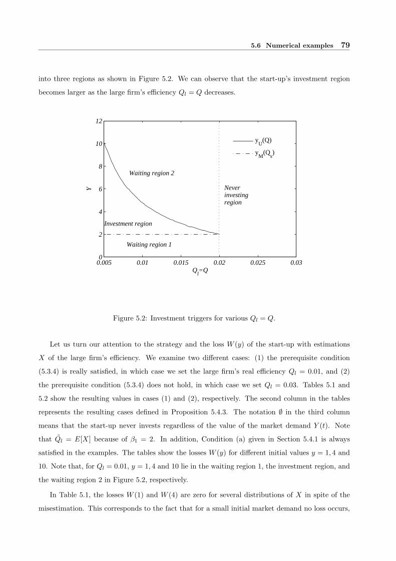
5.6 Numerical examples 79
into three regions as shown in Figure 5.2. We can observe that the start-up’s investment region
becomes larger as the large firm’s efficiency Ql = Q decreases.
0.005 0.01 0.015 0.02 0.025 0.030
2
4
6
8
10
12
Ql=Q
Y
yU
(Q)
yM
(Qs)
Waiting region 2
Waiting region 1
Investment region
Neverinvestingregion
Figure 5.2: Investment triggers for various Ql = Q.
Let us turn our attention to the strategy and the loss W (y) of the start-up with estimations
X of the large firm’s efficiency. We examine two different cases: (1) the prerequisite condition
(5.3.4) is really satisfied, in which case we set the large firm’s real efficiency Ql = 0.01, and (2)
the prerequisite condition (5.3.4) does not hold, in which case we set Ql = 0.03. Tables 5.1 and
5.2 show the resulting values in cases (1) and (2), respectively. The second column in the tables
represents the resulting cases defined in Proposition 5.4.3. The notation ∅ in the third column
means that the start-up never invests regardless of the value of the market demand Y (t). Note
that Ql = E[X] because of β1 = 2. In addition, Condition (a) given in Section 5.4.1 is always
satisfied in the examples. The tables show the losses W (y) for different initial values y = 1, 4 and
10. Note that, for Ql = 0.01, y = 1, 4 and 10 lie in the waiting region 1, the investment region, and
the waiting region 2 in Figure 5.2, respectively.
In Table 5.1, the losses W (1) and W (4) are zero for several distributions of X in spite of the
misestimation. This corresponds to the fact that for a small initial market demand no loss occurs,

80 Chapter 5 Real Options under Incomplete Information
which is shown in Proposition 5.4.3 and Corollary 5.4.1. For a large initial market demand, com-
paring W (10) = 1.55, 0.41 and 0.23, 0.097 in Table 5.1 suggests that the loss in the overestimation
case (O.3) is smaller than that in the underestimation case (U.3). Taking into account that the
value in the case of complete information is V (10, 0.01) = 0.55, even a small estimation error (in
particular, in the underestimation case) causes a serious problem to the start-up. Indeed, the losses
W (10) = 1.55 and 0.41 correspond to 280 and 75 percents of V (10, 0.01) = 0.55, respectively. In
the case where the prerequisite condition does not hold, on the other hand, a small estimation error
causes no problem to the start-up. This can be seen from W (y) = 0 in many rows above and below
X = Ql = 0.03 in Table 5.2. In fact, the start-up can make a correct judgement of never investing
even if it has a small estimation error.
From the above observation, we obtain the following implications about the start-up’s invest-
ment policy under incomplete information. The start-up needs more accurate estimation of the
large firm’s efficiency in the case where it tries to invest than in the case of never investing. In
addition, the start-up that attempts to invest should make a modest estimate because the loss in
the underestimation case is likely to be much larger than that in the overestimation case. The
start-up’s strategy in the underestimation case may cause a loss larger than the project value in
the case of complete information, and therefore its confident investment policy is excessively risky.
Finally, we show interesting numerical comparative static results with respect to the volatility
σ in the underlying market demand Y (t). We set the large firm’s efficiency Ql = 0.01. Figure
5.3 illustrates the start-up’s value function V (y; Ql = 0.01) in the case of complete information for
σ = 0, 0.1, 0.2 and 0.3. For an initial value around the investment region (approximately [1.5, 4.5]
in Figure 5.3) a lower volatility generates a higher value of the start-up’s investment, while for
an initial value in the waiting regions (especially, the waiting region 2 such as y ≈ 10) a higher
volatility is beneficial to the start-up.
This result is intuitive. Note that the possibilities of both firm’s entries in the waiting regions
become smaller as the volatility in the market becomes lower. In other words, the value of the
option to delay the investment is monotonic with respect to the volatility in the market. Then, a
lower volatility has both positive and negative effects on the start-up. The positive one is that a
lower volatility leads the large firm to delay its entry. The negative one is that a lower volatility
decreases the start-up’s option value of waiting. Since around the investment region the start-up
can invest soon even if the volatility in the market is small, the negative effect in the start-up’s
waiting region is not important. As a result, around the investment region, a lower volatility

5.7 Conclusion 81
increases the start-up’s value by the positive effect. Far from the investment region, on the other
hand, the negative effect is dominant, because the start-up tends to wait for a long time until
its investment. In consequence, far from the investment region, a lower volatility decreases the
start-up’s value by the negative effect.
Figure 5.4 illustrates the relative loss W (y)/V (y; Ql) of the start-up with incomplete information
X = [0.005, 0.01] and [0.01, 0.015] for various values of σ. As shown in Proposition 5.4.3 and
Corollary 5.4.1, the relative loss is zero for a small initial value y in Figure 5.4. Observe that, for a
large initial value y, the relative loss is constant with respect to y. This is because W (y)/V (y; Ql)
equals (B(Ql) − B(Ql))yβ2/B(Ql)yβ2 = (B(Ql) − B(Ql))/B(Ql) by Proposition 5.4.3. In Figure
5.4, a lower volatility increases both the relative loss W (y)/V (y; Ql) and the absolute loss W (y).
We observed that the same property holds for most other parameter values than the presented
example.
We can interpret this property as follows. The start-up’s investment decision involves two
different types of uncertainty; namely the market volatility and the estimation of the large firm’s
efficiency. Intuitively, in the market with high volatility, a small estimation error does not make a
big difference in the loss. However, if the uncertainty in the market demand is less, the start-up’s
payoff is more decisively determined by its investment policy. Naturally, the start-up also needs to
take a more accurate investment policy.
5.7 Conclusion
This chapter has investigated the effect of incomplete information in the model in which a start-
up with a unique idea and technology pioneers a new market that will be taken over by a large
firm eventually. The main contribution of this chapter is to evaluate the start-up’s loss due to
incomplete information about the large firm. The proposed method could be applied in other real
options models involving several firms. The results obtained in this chapter can be summarized as
follows.
If the start-up’s efficiency is much better than that of the large firm and the current market
demand cannot generate great profit immediately, then the start-up requires no further survey
on the large firm’s efficiency. On the other hand, information about the large firm’s efficiency is
valuable in the market that can readily generate great profit, even if the start-up’s efficiency is
much better than that of the large firm. In this case, it is quite likely that the start-up’s immediate
investment does not produce much income for the start-up before the large firm’s entry.

82 Chapter 5 Real Options under Incomplete Information
Table 5.1: The loss for uniform distributions X and Ql = 0.01.
X Case Investment region W (1) W (4) W (10)
[0.0025, 0.0075] (U.3) [2, 10.14] 0 0 1.55
[0.005, 0.01] (U.3) [2, 6.57] 0 0 0.41
Ql = 0.01 (C) [2, 4.77] 0 0 0
[0.01, 0.015] (O.3) [2, 3.69] 0 0.089 0.097
[0.0125, 0.0175] (O.3) [2, 2.95] 0 0.36 0.23
[0.015, 0.02] (O.3) [2, 2.42] 0 0.58 0.34
[0.0175, 0.0225] (O.2) ∅ 0.13 1 0.55
[0.02, 0.025] (O.2) ∅ 0.13 1 0.55
Table 5.2: The loss for uniform distributions X and Ql = 0.03.
X Case Investment region W (1) W (4) W (10)
[0.0125, 0.0175] (U.2) [2, 2.95] 0.13 0.74 0.37
[0.015, 0.02] (U.2) [2, 2.42] 0.13 0.47 0.23
[0.0175, 0.0225] (U.1) ∅ 0 0 0
[0.02, 0.025] (U.1) ∅ 0 0 0
[0.0225, 0.0275] (U.1) ∅ 0 0 0
[0.025, 0.03] (U.1) ∅ 0 0 0
Ql = 0.03 (C) ∅ 0 0 0
[0.03, 0.035] (O.1) ∅ 0 0 0
[0.0325, 0.0375] (O.1) ∅ 0 0 0
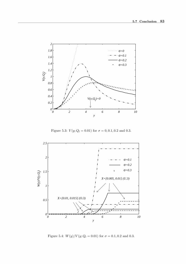
5.7 Conclusion 83
0 2 4 6 8 100
0.2
0.4
0.6
0.8
1
1.2
1.4
1.6
1.8
2
y
V(y
;Ql)
σ=0
σ=0.1
σ=0.2
σ=0.3
V(y;Ql)=0
Figure 5.3: V (y; Ql = 0.01) for σ = 0, 0.1, 0.2 and 0.3.
0 2 4 6 8 100
0.5
1
1.5
2
2.5
y
W(y
)/V
(y;Q
l)
X=[0.01, 0.015] (O.3)
σ=0.1
σ=0.3
X=[0.005, 0.01] (U.3)
x
σ=0.2
Figure 5.4: W (y)/V (y; Ql = 0.01) for σ = 0.1, 0.2 and 0.3.

84 Chapter 5 Real Options under Incomplete Information
When it is doubtful that the start-up’s efficiency overwhelms that of the large firm, information
about the large firm’s efficiency is always valuable regardless of the current market demand. The
reason for this is that there is a possibility that the investment opportunity for the start-up does
not exist in the market, in addition to the same risk as in the previous case, that is, the possibility
that the start-up obtains little profit before the large firm’s entry.
Furthermore, under incomplete information, the expected payoff of the start-up investing at
the zero-NPV trigger could become greater than that of the start-up following the real options
approach. In numerical examples, we have also observed some interesting features of the loss due
to incomplete information such as the property that the loss in the overestimation case tends to be
smaller than that in the underestimation case.
In the real world, a small entrepreneurial firm that has a unique idea and technology but is
not competitive in the market may want to sell its idea and technology to a large firm, rather
than pioneering the market by itself. Then, the value function which the start-up believes can be
interpreted as a reward which the start-up demands for its idea and technology. As revealed in this
chapter, the value of the investment which the start-up believes under incomplete information is
generally different from the real value of the investment. Because of this gap, negotiations between
the start-up and the large firm may not go smoothly. It remains as an interesting issue of future
research to reveal the effect of incomplete information in such a negotiation problem of a firm
having an option to sell its idea and technology to the rival firm.

Chapter 6
Real Options under Asymmetric
Information
6.1 Introduction
This chapter focuses on agency conflicts between the owner and the manager in a decentralized
firm. While most literatures (cf., Sections 4.1 and 5.1) have focused on the strategic interaction
with rival firms, Grenadier and Wang [31] investigated investment timing in a decentralized firm
where the owner (principal) delegates the investment decision to the manager (agent) who holds
private information by combining the real options approach and contract theory (for contract theory,
see the standard textbook [11]). In their model, asymmetric information changes the investment
behavior of the firm from the first-best no-agency case because the owner designs the contract
to provide bonus-incentive for the manager to truthfully reveal private information. Similar real
options models with agency conflicts have been also studied in [8, 56].
Although these models consider only the carrot (i.e., giving bonus-incentive to the manager) as
a measure to deal with agency conflicts, the owner can usually use not only the carrot, but also the
stick (i.e., auditing and fining the manager). Naturally, the impact of auditing has been clarified
in other contexts (e.g., [1, 85]).
In this chapter, we incorporate an auditing mechanism into a model following [31]. As far as the
purpose of the chapter is concerned, we limit their original setup involving both hidden information
and action to only the case of hidden information. We assume that the owner can utilize an auditing
system that fines the manager when a false report is detected, where the higher the cost the owner
pays in auditing, the greater becomes the probability of detection. We show that the optimal

86 Chapter 6 Real Options under Asymmetric Information
contract is determined among three feasible types of contracts: the bonus-incentive only mechanism,
the joint bonus-incentive and auditing mechanism, and the auditing only mechanism. This is
according to the relation between the auditing cost and the amount of the penalty. Although a
similar auditing technology is introduced in [79], the findings in this chapter are more comprehensive
and help connect previous results in this area. Indeed, our solution includes the results of [31] in
the bonus-incentive only region, the results of [79] in the joint bonus-incentive and auditing region,
and the first-best no-agency solution as the limit of the auditing only region.
Furthermore, our results also give good account of the real life relationship between audit and
bonus-incentive as follows. In the case where the manager may commit seriously outright frauds
such as embezzlement, the owner tries to prevent the manager’s offense by using only audit, and
stern punishment by the law improves the social welfare. On the other hand, in the case where
the manager’s private benefit is not necessarily illegal, the owner is likely to prefer a bonus system
such as stock options, and an owner’s too great demand may decrease the social benefit.
The chapter is organized as follows. Section 6.2 provides a brief review of [31]. Section 6.3
incorporates the auditing technology into the model and derives the owner’s optimal contract after
allowing for audit. The final section discusses economic implications of our results involving both
audit and bonus-incentive. Section 6.4 concludes this chapter.
6.2 Preliminaries
This section provides a brief review of the results in [31]. First, let us explain the setup. We
consider a decentralized firm that faces the investment timing decision of a single project. We
assume that the owner (principal) delegates the decision to the manager (agent) and that both the
owner and the manager are risk neutral. Then, in this chapter, the discout factor r(> µ) is equal
to the risk-free rate. While both the owner and the manager know the investment cost I, the value
of the project consists of two components, namely the value Y (t) that is observable to both the
owner and the manager, and the value θ that is privately observed only by the manager. Thus, the
total value of the project is Y (t) + θ. For simplicity, we assume that the observable value Y (t) at
time t obeys the geometric Brownian motion (4.2.1) defined in Section 4.2.
The private component θ potentially takes on two possible values, θ1 or θ2, with 0 ≤ θ2 < θ1 < I.
We denote ∆θ = θ1 − θ2. Before contracting, both the owner and the manager know that the
probability of drawing a higher quality project θ1 equals κ. Immediately after making a contract
with the owner at time 0, the manager privately observes whether the project is of a higher quality

6.2 Preliminaries 87
θ1 or a lower quality θ2. Although the manager’s one-time effort, which cannot be observed by the
owner, changes the likelihood κ in [31], we exclude the effect of the hidden action from the original
setup.
As a benchmark, we examine the case where there is no delegation of the exercise decision and
the owner observes the true value of θ. In this case, the owner’s problem with given θ = θi (i = 1, 2)
becomes the following optimal stopping problem:
U(y; θi) = supτi∈T
E[e−rτi(Y (τi) + θi − I)]. (6.2.1)
Recall that y is the initial value Y (0) and T is a set of all Ft stopping times (see Section 4.2). In
this chapter, it is always assumed that the initial value y is sufficiently low so that the firm has
to wait for its exercise condition to be met. Using the standard method (see [22]), we obtain the
value function U(y; θi) and the optimal stopping time τ∗i of problem (6.2.1) for θ = θi as follows:
U(y; θi) =(
y
y∗i
)β1
(y∗i + θi − I)
τ∗i = inft ≥ 0 | Y (t) ≥ y∗i
y∗i =β1
β1 − 1(I − θi). (6.2.2)
Recall that β1 = β10 is the characteristic root defined by (4.2.12).
The threshold y∗i is the optimal investment trigger for the owner who observes the value θi at
time 0. Thus, the ex ante value of the owner’s option in the first-best no-agency setting (denoted
π∗o(y)) becomes:
π∗o(y) = κU(y; θ1) + (1 − κ)U(y; θ2)
= κ
(y
y∗1
)β1
(y∗1 + θ1 − I) + (1 − κ)(
y
y∗2
)β1
(y∗2 + θ2 − I). (6.2.3)
Now, let us turn to the principal-agent setting without auditing. In this case, the owner has the
option to invest, but delegates the exercise decision to the manager. At time 0, the owner offers the
manager a contract that commits the owner to pay the manager at the time of exercise. We assume
no opportunity for renegotiation exists. Although the commitment may lead to ex post inefficiency
in investment timing, it increases the ex ante value of the project. In fact, if the owner makes no
contract with the manager, the owner’s ex ante option value becomes (6.2.3) with q = 0. This is
because the manager hands the owner θ2 and makes θ1 − θ2 his/her own when the true value is θ1.
As discussed in [31], the optimal contract is included in a mechanism MGW = (yi, wi) | i = 1, 2
in which the owner pays the manager the bonus wi at the investment time when the manager
88 Chapter 6 Real Options under Asymmetric Information
exercises the investment at time τi = inft ≥ 0 | Y (t) ≥ yi. Here the superscript “GW” refers
to the solution of [31]. Since the revelation principle (see [11]) ensures that the manager who
observes θi faithfully invests at the trigger yi, the optimal contract is the solution of the problem
of maximizing the owner’s ex ante option value of the investment:
maximizeyi,wi κ
(y
y1
)β1
(y1 + θ1 − I − w1) + (1 − κ)(
y
y2
)β1
(y2 + θ2 − I − w2)
subject to κ
(y
y1
)β1
w1 + (1 − κ)(
y
y2
)β1
w2 ≥ 0
wi ≥ 0 (i = 1, 2)(y
y1
)β1
w1 −(
y
y2
)β1
(w2 + ∆θ) ≥ 0(y
y2
)β1
w2 −(
y
y1
)β1
(w1 − ∆θ) ≥ 0,
(6.2.4)
where yi > y. In the constraints of problem (6.2.4), the first and second inequalities correspond
to the ex ante participation constraint and the ex post limited-liability constraints, respectively,
while the last two inequalities are the ex post incentive-compatibility constraints. The incentive-
compatibility constraint means that with a truthful report, the manager who observes θ = θ1
(resp. θ = θ2) obtains the expected payoff (y/y1)β1w1 (resp. (y/y2)β1w2), which is larger than the
expected payoff for a false report, (y/y2)β1(w2 + ∆θ) (resp. (y/y1)β1(w1 − ∆θ)).
In problem (6.2.4), it can be shown that the bonus w2 = 0 and only the third inequality (i.e.,
the incentive-compatibility condition for the manager who observes the better project value θ1)
binds. Then, the optimal solution (yGWi , wGW
i ) | i = 1, 2 becomes:
(yGW1 , wGW
1 ) =
(y∗1,
(y∗1
yGW2
)β1
∆θ
)(6.2.5)
(yGW2 , wGW
2 ) =(
β1
β1 − 1
(I − θ2 +
κ∆θ
1 − κ
), 0
). (6.2.6)
For further details, see the solution for the hidden information only region in [31]. It is worth
noting that the trigger for the higher quality project, yGW1 , remains unchanged from the first-best
trigger y∗1 defined by (6.2.2), while the trigger for the lower quality project, yGW2 , is larger than
the first-best trigger y∗2 defined by (6.2.2). This is because the owner attempts to decrease the
information rent to the manager who observes the higher quality project by deferring investment
timing for the lower quality project. The owner’s and manager’s ex ante option values, πGWo and
πGWm , respectively, are obtained by substituting the optimal solution (yGW
i , wGWi ) | i = 1, 2 into
the objective function and the right-hand side of the first inequality of the constraints of problem
(6.2.4).
6.3 Theoretical results 89
This is the result in the hidden information case of [31]. In the next section, we extend their
analysis to a case allowing the owner to audit the manager at a cost.
6.3 Theoretical results
This section derives the optimal contract involving bonus-incentive and audit. The owner detects
the real value of θ at probability di by paying the auditing cost c(di) for the manager’s report
θ = θi when the manager executes the project. We assume that the manager is fined the penalty
Γ(> 0) for cheating when a false report is detected. In general, as discussed in [2], the society could
suffer different damages, according to the types of the punishment. However, we do not have to
care whether the owner can receive the total amount of the fine, Γ from the manager, or whether
a part of Γ represents the manager’s disutility from other punishment such as dismissal from the
managerial post. This is because the manager does not in any case cheat the owner in the optimal
contract in our setting.
Here, the cost function c(di) and the penalty Γ are given exogenously. We assume that the cost
function c(di) satisfies conditions:
c(0) = 0, (6.3.1)
limdi↑1
c(di) = +∞, (6.3.2)
c′(di) > 0 (di ∈ [0, 1)), (6.3.3)
c′′(di) > 0 (di ∈ [0, 1)). (6.3.4)
The conditions (6.3.1) and (6.3.3) are explicit from the property of auditing. The assumption
(6.3.2) is realistically intuitive because no auditing can always detect the manager’s false report.
The condition (6.3.4), which is a little bit technical, ensures the convexity of the cost function.
In this setting, the contract is designed as a mechanism MA = (yi, wi, di) | i = 1, 2, where
the auditing level di for the manager’s report θ = θi is added to the mechanism MGW. Here the
superscript “A” refers to the solution of the setting allowing audit. The optimal contract to the
90 Chapter 6 Real Options under Asymmetric Information
owner becomes the solution of the following problem:
maximizeyi,wi,diκ
(y
y1
)β1
(y1 + θ1 − I − w1 − c(d1)) + (1 − κ)(
y
y2
)β1
(y2 + θ2 − I − w2 − c(d2))
subject to κ
(y
y1
)β1
w1 + (1 − κ)(
y
y2
)β1
w2 ≥ 0
wi ≥ 0 (i = 1, 2)
di ≥ 0 (i = 1, 2)(y
y1
)β1
w1 −(
y
y2
)β1
(w2 + ∆θ − d2Γ) ≥ 0(y
y2
)β1
w2 −(
y
y1
)β1
(w1 − ∆θ − d1Γ) ≥ 0,
(6.3.5)
where yi > y. The first two constraints of problem (6.3.5) are the same as those of problem (6.2.4),
while the incentive-compatibility constraints of problem (6.3.5) include an additional term, the
expected penalty diΓ. It can be easily checked that the revelation principle holds in this case,
as in the previous setting, even if the penalty Γ is counted in the owner’s profit. Therefore, the
owner does not make any contract to allow the manager to report untruthfully. Let us check this
revelation principle. Assume that the owner makes the contract (yi, wi, di) | (i = 1, 2) that
leads the manager who observes the higher quality θ1 to falsely report θ2, and the manager who
observes the lower quality θ2 to truthfully report θ2. Then, the owner obtains the expected payoff
(y/y2)β1(y2 + θ2 − I − w2 + κd2Γ − c(d2)), but the same expected payoff can be realized by a
feasible solution (y1, w1, d1) = (y2, w2 + ∆θ − d2Γ, d2), (y2, w2, d2) = (y2, w2, d2) of problem (6.3.5).
Similarly, we can show that the owner’s expected payoffs in other types of contracts allowing the
manager’s dishonest behavior are dominated by the maximum value of problem (6.3.5). Thus,
the revelation principle always holds, and we only have to derive the optimal solution of problem
(6.3.5).
Proposition 6.3.1 The optimal contract (yAi , wA
i , dAi ) | i = 1, 2 in the setting with auditing is
given as follows:
Case (I): 0 < Γ ≤ (1 − κ)c′(0)/κ (bonus-incentive only region)
(yA1 , wA
1 , dA1 ) = (y∗1, w
GW1 , 0)
(yA2 , wA
2 , dA2 ) = (yGW
2 , 0, 0),
Case (II): (1 − κ)c′(0)/κ < Γ ≤ max∆θ, (1 − κ)c′(∆θ/Γ)/κ (joint bonus-incentive and auditing

6.3 Theoretical results 91
region)
(yA1 , wA
1 , dA1 ) =
(y∗1,
(y∗1yA2
)β1
(∆θ − dA2 Γ), 0
)
(yA2 , wA
2 , dA2 ) =
(β1
β1 − 1
(I − θ2 +
κ
1 − κ(∆θ − dA
2 Γ) + c(dA2 )
), 0,
(c′
)−1(
κΓ1 − κ
)),
Case (III): Γ > max∆θ, (1 − κ)c′(∆θ/Γ)/κ (auditing only region)
(yA1 , wA
1 , dA1 ) = (y∗1, 0, 0)
(yA2 , wA
2 , dA2 ) =
(β1
β1 − 1(I − θ2 + c(dA
2 )), 0,∆θ/Γ)
.
Proof Note that in problem (6.3.5), the first constraint is induced by the second constraints wi ≥
0 (i = 1, 2), and yβ1 can be ignored. We solve the problem (6.3.5) without the final constraint (the
incentive-compatibility constraint for the manager who observes the bad value θ = θ2), and then
also check that the obtained solution satisfies the removed constraint. Let (yAi , wA
i , dAi ) | i = 1, 2
be the optimal solution of problem (6.3.5) without the final constraint. It immediately follows that
wA2 = 0, dA
1 = 0, and (1yA1
)β1
wA1 −
(1yA2
)β1
(∆θ − dA2 Γ) = 0. (6.3.6)
Let λi (i = 1, 2, 3) denote the Lagrangian multipliers associated with the remaining constraints
w1 ≥ 0, d2 ≥ 0, and (6.3.6), respectively. That is, we form the Lagrangian:
L(y1, y2, w1, d2) = κ
(1y1
)β1
(y1 + θ1 − I − w1) + (1 − κ)(
1y2
)β1
(y2 + θ2 − I − c(d2))
+λ1w1 + λ2d2 + λ3
((1y1
)β1
w1 −(
1y2
)β1
(∆θ − d2Γ)
).
The Karush-Kuhn-Tucker conditions are (6.3.6),
∂L∂y1
= κ
((−β1 + 1)
(1yA1
)β1
− β1(θ1 − I − wA1 )
(1yA1
)β1+1)
− λ3β1wA1
(1yA1
)β1+1
= 0, (6.3.7)
∂L∂y2
= (1 − κ)
((−β1 + 1)
(1yA2
)β1
− β1(θ2 − I − c(dA2 ))
(1yA2
)β1+1)
+ λ3β1(∆θ − dA2 Γ)
(1yA2
)β1+1
= 0,
(6.3.8)∂L∂w1
= −κ
(1yA1
)β1
+ λ1 + λ3
(1yA1
)β1
= 0, (6.3.9)
∂L∂d2
= −(1 − κ)c′(dA2 )
(1yA2
)β1
+ λ2 + λ3Γ(
1yA2
)β1
= 0, (6.3.10)

92 Chapter 6 Real Options under Asymmetric Information
and
λ1wA1 = λ2d
A2 = 0, λi ≥ 0 (i = 1, 2, 3). (6.3.11)
Let us now derive the solution of (6.3.6)–(6.3.11), depending on whether λi equals zero. If
λ1 = λ2 = 0, we have λ3 = κ and the solution in Case (II). If λ1 > 0 and λ2 = 0, from (6.3.6)–
(6.3.10) we have the solution in Case (III) with
λ1 =(
1yA1
)β1(
κ − (1 − κ)c′(dA2 )
Γ
)and
λ3 =(1 − κ)c′(dA
2 )Γ
.
If λ1 = 0 and λ2 > 0, we obtain the solution in Case (I) with
λ2 =(
1yA2
)β1
((1 − κ)c′(0) − κΓ)
and
λ3 = κ.
If λi > 0 (i = 1, 2), from (6.3.6) we have ∆θ = 0, which contradicts ∆θ > 0. Taking into account
that the conditions λi ≥ 0 (i = 1, 2, 3), dA2 < 1 that results from limd2↑1 c(d2) = +∞, and the
condition under which the solution of c′(dA2 ) = κΓ/(1−κ) exists, we can show that for a given Γ, the
solution satisfying the Karush-Kuhn-Tucker conditions (6.3.6)–(6.3.11) is uniquely determined as
the statement of Proposition 6.3.1. Furthermore, the solution explicitly satisfies the final constraint
in problem (6.3.5). 2
In Proposition 6.3.1, and as intuitively expected, the owner neither gives any bonus for the
manager’s bad report θ2 nor audits the manager’s good report θ1. The investment trigger of the
high quality project does not change from that of the no-agency setting as in the result by [31].
However, the other components of the contract and the owner’s strategy changes, depending on the
auditing cost c(di) and the amount of the penalty, Γ. Indeed, the contract is classified into three
regions. The solution changes from Case (I) to Case (III) via Case (II) as the penalty Γ becomes
larger, as observed in Figures 6.1 and 6.2. In the numerical example, we set the parameter values
α = 0, r = 0.04, σ = 0.2, and I = 1 as in [22], and set y = 0.5, θ1 = 0.5, θ2 = 0, κ = 0.5, and
c(di) = 0.5di/(1 − di). Figure 6.1 depicts the expected discounted cost of the bonus and auditing,
(y/yA1 )β
1wA1 , (y/yA
2 )β1 c(dA
2 ), together with the investment trigger yA2 . We do not illustrate quantities
yA1 , wA
2 , and dA1 because of yA
1 = y∗1, wA2 = dA
1 = 0.

6.3 Theoretical results 93
Case (I) is likely to hold if the marginal cost of auditing is high relative to the penalty Γ, or
if the probability of drawing the better project θ1 is low. In this case, the owner pays the whole
information rent to the manager without auditing, since the auditing technology does not work
at all. Conversely, in Case (III), where the penalty is severe and the auditing cost is not so high,
the owner uses only the auditing system without giving any bonus to the manager. Case (II) is
the intermediate case. In this case, both bonus-incentive and audit are effective by the trade-off
between the auditing cost and the amount of the penalty.
Let us explain the relation between Proposition 6.3.1 and the results from previous studies.
The solution in Case (I) coincides with that of [31], i.e., (6.2.5) and (6.2.6). Then, it is readily seen
that y∗2 < yA2 ≤ yGW
2 , πGWo (y) ≤ πA
o (y) < π∗o(y), and πA
m(y) ≤ πGWm (y), where πA
o and πAm denote
the owner’s and manager’s ex ante option values defined by
πAo (y) = κ
(y
y∗1
)β1
(y∗1 + θ1 − I − wA1 ) + (1 − κ)
(y
yA2
)β1
(yA2 + θ2 − I − c(dA
2 ))
πAm(y) = κ
(y
y∗1
)β1
wA1 .
Note that πAo and πA
m are exactly the same as πGWo and πGW
m , respectively, in Case (I). If we assume
that Γ = ∆θ and c′(0) = 0, the solution is classified into Case (II) and agrees with that of [79]
where the owner can control the penalty Γ to a limit ∆θ. Moreover, the solution in Case (III)
converges to that of the first-best no-agency case by letting Γ → +∞. This appears to correspond
to Proposition 4 in [1].
We can see from Figure 6.1 that yA2 monotonically decreases to y∗2 = 2 for penalties Γ. Figure
6.2 indicates that the owner’s (resp. manager’s) ex ante option value πAo (resp. πA
m) monotonically
increases (resp. decreases) for Γ. These results can also be easily proved, and therefore the proofs
are omitted. In particular, the monotone increase in the owner’s option value with respect to the
amount of the penalty is consistent with the maximal punishment principle (see [1, 79]). That is,
the owner imposes the maximum penalty if he/she can determine the penalty within some limit.
Following [31], we define the social loss πAloss by
πAloss = π∗
o − (πAo + πA
m).
It should be noted that the social loss πAloss does not need to involve the social cost of the punish-
ment, which varies between different kinds of punishment as mentioned in [2], since the optimal
contract precludes cheating. The social loss πAloss, unlike the owner’s option value, is not necessar-
ily monotonic for Γ as observed in Figure 6.2, although for sufficiently large Γ, it monotonically

94 Chapter 6 Real Options under Asymmetric Information
decreases to zero (cf. Proposition 4 in [1]). This means that a halfway penalty could only be of
benefit to the owner and brings with it inefficiency in terms of social surplus, while a severe penalty
improves social efficiency.
6.4 Economic insights
This section gives the motivation of considering both audit and bonus-incentive in the contract
described in the previous section as well as the economic insights extracted from the results we
obtained in the previous section. To do so, we shall place our discussion in a real-life context.
In practice, it is common that firms employ independent auditing systems in addition to their
internal ones. There are three types of independent audits, that is, financial statement audit,
operational audit, and compliance audit. We shall now relate our results to the cases of financial
statement audit and operational audit.
By the means of financial statement audit, the owner can ensure the accuracy of the firm’s
financial statements in its business report. In other words, the owner attempts to prevent the
manager from making false statements regarding the firm’s financial status and figures. When
the manager’s outright frauds such as window-dressing settlement and embezzlement are detected
by the audit, the manager is severely punished by the relevant law (e.g., The Commercial Code,
The Corporation Law, The Securities and Exchange Law, The Penal Code, etc. in the case of
Japan). A well-known example is the WorldCom scandal in which its managers were punished for
its window-dressing settlement which led to higher reported profits than the actual profits. Another
example is the Aramark case in which its managers were charged with the embezzlement involving
underreporting of the company’s vending machine revenues.
For this kind of audit, the penalty Γ is expected to be much larger than ∆θ, since Γ includes
not only the compensation but also further punishment by the law. Hence, we believe that Case
(III) in Proposition 3.1 is appropriate for this situation, even if the auditing cost c is somewhat
high. Here, the owner simply tries to set the auditing level high enough to prevent the manager
from making false financial statements. Another logical finding we obtained under Case (III) is
that severe penalty Γ brings small social loss πAloss (see Figure 6.2).
On the other hand, Cases (I) and (II) are more likely to apply to operational audit than financial
statement audit. The purpose of operational audit is usually to assess the manager’s efficiency,
instead of detecting explicitly illegal frauds of the manager. When the manager’s inefficient waste
is pointed out by the audit, the owner can force the manager to make improvements by transferring

6.4 Economic insights 95
0 1 2 3 4 50
0.005
0.01
0.015
0.02
0.025
0.03
0.035
Γ
0.01y2A
(y/y1A)β1 w
1A
(y/y2A)β1 c(d
2A)
Case (II)Case (I) Case (III)
Figure 6.1: yA2 , wA
1 and c(dA2 ) for penalties Γ.
0 1 2 3 4 50
0.002
0.004
0.006
0.008
0.01
Γ
0.1πoA(y)
πmA(y)
πAloss
(y)
Case (III)Case (I) Case (II)
Figure 6.2: πAo (y), πA
m(y) and πAloss for penalties Γ.
96 Chapter 6 Real Options under Asymmetric Information
a portion of the manager’s profit to the owner. That is, in this case, Γ can be interpreted as the
owner’s punishment imposed on the manager rather than the punishment by the law. The owner
cannot claim Γ larger than ∆θ, because the manager’s act is not necessarily illegal in this case.
Accordingly, it is quite likely that the owner prefers the bonus system to operational audit depending
on the auditing cost. The bonus system often takes the form of stock options in real life. Note
that in this situation the social welfare may be lost if the owner demands too much profit from the
manager who does not execute any illegal fraud. This intuition is captured by our results in Case
(II) where the social loss πAloss does not necessarily show a monotone decrease with respect to Γ
(see Figure 6.2).
6.5 Conclusion
In this chapter, we investigated the effects of both audit and bonus-incentive as a measure to deal
with agency conflicts between the owner and the manager with private information. We showed that
the owner’s optimal contract is determined among three feasible types of contracts, according to
the relation between the auditing cost and the amount of the penalty. This solution not only helps
unify several previous results in this area, but also give good account of the real life relationship
between audit and bonus-incentive.

Chapter 7
Conclusion
In this thesis, we have shown new results about the duality and bounds on risk-neutral probabilities
in option pricing based on prices of other derivatives. Furthermore, in the context of strategic real
options, we have analyzed (i) the option to choose both the type and the timing of the projects,
(ii) the loss due to incomplete information about the competitor, and (iii) the bonus and audit
system to deal with agency conflicts between the owner and the manager. The results obtained in
this thesis are summarized as follows:
(Chapter 2) We clarified financial meanings of duality in the problem of finding the derivative
price range from the observed prices of other derivatives in terms of the buy-and-hold hedging.
(Chapter 3) We derived analytical bounds on risk-neutral cumulative distribution functions of
the underlying asset price from the observed prices of call and put options. Moreover, we
computed the bounds from the Nikkei 225 option data in Japan so that we could capture the
property of the bounds.
(Chapter 4) We investigated the simultaneous effects of the competition on the investment timing
and the choice of the project type in the context of R&D investment. In particular, we showed
that a lower-standard technology is likely to appear for the reason that the preemption game
due to the competition hastens the investment timing.
(Chapter 5) We evaluated the start-up’s loss due to incomplete information about the efficiency
of the large firm that subsequently takes over the market from the start-up. We elucidated
in which cases and how greatly the firm suffers the loss due to incomplete information.
(Chapter 6) We studied the problem of the owner who designs the contract consisting of bonus
and audit so that the manager with private information makes investment at efficient timing.

98 Chapter 7 Conclusion
The optimal contract is determined among three feasible types of contracts, depending on
whether the audit is effective or not, and whether the manager’s private benefit is legal or
illegal. The result connects previous works in this area because the result for each type of
contracts includes a previous result.
As we summarized above, we have made several contributions to the study on financial and real
options. However, there are some problems that remain unsolved. In the following, we give some
future issues related to each section of the thesis.
(Chapters 2 and 3) Sections 2 and 3 treated only European type derivatives. As of now, similar
results have yet to be obtained for American type derivatives. As shown in Section 2, the
problem of finding the derivative price range from the observed prices of other derivatives
is equivalent to the problem of hedging the derivative with a buy-and-hold portfolio. In
most cases, we cannot practice complete dynamic hedging for complicated derivatives such
as American type derivatives. Thus, providing a simple hedging strategy for American type
derivatives, which is easy to execute, will be very useful in practice.
(Chapter 4) The R&D investment often takes a form of multi-step investment, though Section
4 did not consider such a case. This is because the multi-step investment reduces the risk
in R&D projects which is much higher than that in other projects. However, a large-scale
investment in a lump may be favored by a firm with the fear of preemption by the competitor.
So far, no studies have clarified the effects of the competition on a multi-step R&D investment.
(Chapter 5) Section 5 did not consider the situation where the large firm buys out the small
entrepreneur. It is an interesting issue to investigate how incomplete information influences
a firm’s M&A strategy, and in which case and how greatly the firm suffers the loss due to
incomplete information. Recently, M&A has frequently caused a social problem, and therefore
theoretical analysis about M&A needs to be conducted more and more.
(Chapter 6) Section 6 investigated agency conflicts between two players, namely the owner and
the manager, in a single firm. Another important player in corporate finance is the creditor.
By structuring a real options model that captures the relationship of three players, i.e.,
the shareholder (owner), the manager, and the creditor, we will be able to understand the
interactions among financing, the capital structure, and the investment decision.
Appendix A
Appendix of Chapter 4
A.1 The stopping time game and its equilibrium
In this paper, we adopt the concept of the stopping time game introduced in [24] because of its
intuitive simplicity. We make a brief explanation of the concept by [24] below. See [24] for further
details.
The stopping time game proceeds as follows. In the absence of an action by either player, the
game environment evolves according to the stochastic process (4.2.1). If a firm has not invested until
time t, its action set is At = 0, 1, 2, where 0 stands for no entry and 1, 2 for invest in technology
1, 2 respectively. If a firm has already invested before time t, then the action set At is the null.
Investment by one of the firms (called leader) terminates the game and determines the (expected)
payoff of both firms because the other (called follower) necessarily takes the optimal response. We
assume that the simultaneous action yields the expected payoff (L(Y )+F (Y ))/2 to both firms (we
take α = 1/2 in p. 746 in [24]). That is, one of the firms prove to invest infinitesimally earlier than
the other even if both attempt to invest at the same timing. The remaining one must take the
optimal response as a follower. The probability that a firm is chosen as a leader is fair, i.e., 1/2.
A strategy for a firm is generally defined as a mapping from the history of the game Ht to the
action set At. Here, at time t the history Ht has two components: the sample path of the stochastic
process (4.2.1) and the actions of two players up to time t. Since the stochastic process (4.2.1)
is Markovian, we restrict attention to Markovian strategies and a Markovian perfect equilibrium.
Then, in equilibrium, at time inft ≥ 0 | Y (t) ≥ yP both firms attempt to invest in technology
i satisfying Li(yP ) ≥ Lj(yP ) for j 6= i. Under the assumption only one of the firms is actually
allowed to invest at time inft ≥ 0 | Y (t) ≥ yP and the other invests at time τ∗Fi
as a follower.

100 Chapter 7 Conclusion
Several studies such as [29, 87] use the above concept by [24], but there is another stream
[42, 82, 83] that has tried to elucidate the possibility of mistaken simultaneous investment. They
introduces a more complex strategy space of the firms, instead of the technical assumption that the
simultaneous action yields the payoff (L(Y ) + F (Y ))/2. Even in their approach, the outcome still
holds true under Assumption A due to rent equalization. They suggest that, without Assumption
A both firms may make simultaneous investment mistakenly, and of course the analysis without
Assumption A is an interesting issue in future research direction.

Bibliography
[1] D. Baron and D. Besanko. Regulation, asymmetric information, and auditing. RAND Journal
of Economics, 15:447–470, 1984.
[2] G. Becker. Crime and punishment: An economic approach. Journal of Political Economy,
76:169–217, 1985.
[3] A. Bernardo and B. Chowdhry. Resources, real options, and corporate strategy. Journal of
Financial Economics, 63:211–234, 2002.
[4] D. Bertsimas and N. Bushueva. Option pricing without price dynamics: a geometric approach.
Working Paper, Massachusetts Institute of Technology, 2004.
[5] D. Bertsimas and N. Bushueva. Option pricing without price dynamics: a probabilistic ap-
proach. Working Paper, Massachusetts Institute of Technology, 2004.
[6] D. Bertsimas and I. Popescu. On the relation between option and stock prices: a convex
optimization approach. Operations Research, 50:358–374, 2002.
[7] T. Bielecki and M. Rutkowski. Credit Risk: Modeling, Valuation and Hedging. Springer, Berlin,
2002.
[8] P. Bjerksund and G. Stensland. A self-enforced dynamic contract for processing of natural
resources. In M. Brennan and L. Trigeorgis, editors, Project Flexibility, Agency, and Compe-
tition, pages 109–127. Oxford University Press, Oxford, 2000.
[9] T. Bjork. Arbitrage Theory in Continuous Time. Oxford University Press, Oxford, 2004.
[10] F. Black and M. Scholes. The pricing options and corporate liabilities. Journal of Political
Economy, 81:637–654, 1973.
[11] P. Bolton and M. Dewatripont. Contract Theory. MIT Press, London, 2005.

102 BIBLIOGRAPHY
[12] J. F. Bonnas and A. Shapiro. Perturbation Analysis of Optimization Problems. Springer, New
York, 2000.
[13] M. Boyer, E. Gravel, and P. Lasserre. Real options and strategic competition: a survey.
Working paper, Universite de Montreal, 2004.
[14] P. Boyle and X. S. Lin. Bounds on contingent claims based on several assets. Journal of
Financial Economics, 46:383–400, 1997.
[15] M. Brennan and E. Schwartz. Evaluating natural resource investments. Journal of Business,
58:135–157, 1985.
[16] P. Dasgupta and J. Stiglitz. Industrial structure and the nature of innovative activity. Eco-
nomic Journal, 90:266–293, 1980.
[17] J. Decamps, T. Mariotti, and S. Villeneuve. Investment timing under incomplete information.
Mathematics of Operations Research, 30:472–500, 2005.
[18] J. Decamps, T. Mariotti, and S. Villeneuve. Irreversible investment in alternative projects.
Economic Theory, 28:425–448, 2006.
[19] E. Derman and I. Kani. Riding on a smile. Risk, 7:32–39, 1994.
[20] A. Dixit. Entry and exit decisions under uncertainty. Journal of Political Economy, 97:620–
638, 1989.
[21] A. Dixit. Choosing among alternative discrete investment projects under uncertainty. Eco-
nomics Letters, 41:265–268, 1993.
[22] A. Dixit and R. Pindyck. Investment Under Uncertainty. Princeton University Press, Prince-
ton, 1994.
[23] B. Dupire. Pricing with a smile. Risk, 7:18–20, 1994.
[24] P. Dutta and A. Rustichini. A theory of stopping time games with applications to product
innovations and asset sales. Economic Theory, 3:743–763, 1993.
[25] S. Fleten and K. Maribu. Investment timing and capacity choice for small-scale wind power
under uncertainty. Working paper, Norwegian University of Science and Technology, 2004.

BIBLIOGRAPHY 103
[26] F. Fornari and A. Mele. Recovering the probability density function of asset prices using garch
as diffusion. Journal of Empirical Finance, 8:83–110, 2001.
[27] D. Fudenberg and J. Tirole. Preemption and rent equalization in the adoption of new tech-
nology. Review of Economic Studies, 52:383–401, 1985.
[28] M. Goto, R. Takashima, M. Tsujimura, and T. Ohno. Entry and exit decisions under uncer-
tainty in a duopoly. Working paper, Waseda University, 2007.
[29] S. Grenadier. The strategic exercise of options: development cascades and overbuilding in real
estate markets. Journal of Finance, 51:1653–1679, 1996.
[30] S. Grenadier. Option exercise games: an application to the equilibrium investment strategies
of firms. Review of Financial Studies, 15:691–721, 2002.
[31] S. Grenadier and N. Wang. Investment timing, agency, and information. Journal of Financial
Economics, 75:493–533, 2005.
[32] S. Grenadier and A. Weiss. Investment in technological innovations: an option pricing ap-
proach. Journal of Financial Economics, 44:397–416, 1997.
[33] B. Grundy. Option prices and the underlying asset’s return distribution. Journal of Finance,
46:1045–1069, 1991.
[34] D. Han, X. Li, D. Sun, and J. Sun. Bounding option prices of multi-assets: a semi-definite
programming approach. Pacific Journal of Optimization, 1:59–79, 2005.
[35] M. Harrison and D. Kreps. Martingales and arbitrage in multiperiod securities markets. Jour-
nal of Economic Theory, 20:381–408, 1979.
[36] M. Harrison and S. Pliska. Martingales and stochastic integrals in the theory of continuous
trading. Stochastic Processes and their Applications, 11:215–260, 1981.
[37] N. Hartvig, J. Jensen, and J. Pedersen. A class of risk neutral densities with heavy tails.
Finance and Stochastic, 5:115–128, 2001.
[38] C. Hennessy and T. Whited. Debt dynamics. Journal of Finance, 60:1129–1165, 2005.
[39] J. Hinloopen. Subsidizing cooperative and noncooperative R&D in duopoly with spillovers.
Journal of Economics, 66:151–175, 1997.

104 BIBLIOGRAPHY
[40] Y. Hsu and B. Lambrecht. Preemptive patenting under uncertainty and asymmetric informa-
tion. Annals of Operations Research, 151:5–28, 2007.
[41] A. Huchzermeier and C. Loch. Project management under risk: using the real options approach
to evaluate flexibility in R&D. Management Science, 47:85–101, 2001.
[42] K. Huisman. Technology Investment: A Game Theoretic Real Options Approach. Kluwer
Academic Publishers, Boston, 2001.
[43] K. Huisman and P. Kort. Strategic investment in technological innovations. European Journal
of Operational Research, 144:209–223, 2003.
[44] K. Huisman and P. Kort. Strategic technology adoption taking into account future techno-
logical improvements: a real options approach. European Journal of Operational Research,
159:705–728, 2004.
[45] J. Hull. Options, Futures, and Other Derivatives. Prentice Hall, New Jersey, 6th edition, 2005.
[46] S. Jewson and A. Brix. Weather Derivative Valuation: The Meteorological, Statistical, Finan-
cial And Mathematical Foundations. Cambridge University Press, Cambridge, 2005.
[47] D. Jorgenson. Capital theory and investment behavior. American Economic Review, 53:247–
259, 1963.
[48] J. Jou and T. Lee. R&D investment decision and optimal subsidy. R&D Management, 31:137–
148, 2001.
[49] S. Kou. Option pricing under a double exponential jump diffusion model. Management Science,
50:1178–1192, 2004.
[50] B. Lambrecht and W. Perraudin. Real options and preemption under incomplete information.
Journal of Economic Dynamics and Control, 27:619–643, 2003.
[51] J. Lee and A. Paxson. Valuation of R&D real american sequential exchange options. R&D
Management, 31:191–201, 2001.
[52] H. Leland. Corporate debt value, bond covenants, and optimal capital structure. Journal of
Finance, 49:1213–1252, 1994.

BIBLIOGRAPHY 105
[53] A. Lo. Semi-parametric upper bounds for option prices and expected payoffs. Journal of
Financial Economics, 19:373–387, 1987.
[54] C. Loch and K. Bode-Greuel. Evaluating growth options as sources of value for pharmaceutical
research projects. R&D Management, 31:231–248, 2001.
[55] G. Loury. Market structure and innovation. Quarterly Journal of Economics, 93:395–410,
1979.
[56] J. Mæland. Valuation of an irreversible investment: private information about a stochastic
investment cost. Working paper, Norwegian School of Economics and Business Administration,
2005.
[57] H. Markowitz. Portfolio selection. Journal of Finance, 7:77–91, 1952.
[58] D. Mauer and A. Triantis. Interactions of corporate financing and investment decisions: A
dynamic framework. Journal of Finance, 49:1253–1277, 1994.
[59] R. McDonald and D. Siegel. The value of waiting to invest. Quarterly Journal of Economics,
101:707–727, 1986.
[60] R. Merton. Theory of rational option pricing. Bell Journal of Economics and Management
Science, 4:141–183, 1973.
[61] R. Merton. On the pricing of corporate debt: The risk structure of interest rates. Journal of
Finance, 29:449–470, 1974.
[62] F. Modigliani and M. Miller. The cost of capital, corporation finance and the theory of
investment. American Economic Review, 48:261–297, 1958.
[63] P. Murto. Exit in duopoly under uncertainty. RAND Journal of Economics, 35:111–127, 2004.
[64] E. Nicolato and E. Venardos. Option pricing under a double exponential jump diffusion model.
Mathematical Finance, 13:445–466, 2003.
[65] M. Nishihara and M. Fukushima. Evaluation of firm’s loss due to incomplete information in
real investment decision. European Journal of Operational Research, forthcoming.
[66] M. Nishihara and T. Shibata. The agency problem between the owner and the manager in
real investment: The bonus-audit relationship. Operations Research Letters, forthcoming.

106 BIBLIOGRAPHY
[67] M. Nishihara, M. Yagiura, and T. Ibaraki. Duality in option pricing based on prices of other
derivatives. Operations Research Letters, 35:165–171, 2007.
[68] B. Øksendal. Stochastic Differential Equations: An Introduction with Applications. Springer,
Berlin, 6th edition, 2003.
[69] M. Perlitz, T. Peske, and R. Schrank. Real options valuation: the new frontier in R&D project
evaluation? R&D Management, 29:255–269, 1999.
[70] A. Perold. Large-scale portfolio optimization. Management Science, 30:1143–1160, 1984.
[71] R. Pindyck. Irreversible investment, capacity choice, and the value of the firm. American
Economic Review, 78:969–985, 1988.
[72] R. Pindyck. Irreversibility, uncertainty, and investment. Journal of Economic Literature,
29:1110–1148, 1991.
[73] M. Rubinstein. Implied binomial trees. Journal of Finance, 49:771–819, 1994.
[74] E. Schwartz and L. Trigeorgis, editors. Real Options and Investment Under Uncertainty:
Classical Readings and Recent Contributions. MIT Press, London, 2004.
[75] A. Shapiro. On duality theory of conic linear problems. Semi-infinite Programming: Recent
Advances, Nonconvex Optimization and Its Applications 57, M. Goberna and M. Lopez, eds.
Kluwer Academic Publication, Dordrecht, 2001.
[76] W. Sharpe. Capital asset prices: A theory of market equilibrium under conditions of risk.
Journal of Finance, 19:425–442, 1964.
[77] W. Sharpe. Asset allocation: Management style and performance measurement. Journal of
Portfolio Management, Winter:7–19, 1992.
[78] T. Shibata. The impacts of uncertainties in the real options model under incomplete informa-
tion. European Journal of Operational Research, forthcoming.
[79] T. Shibata. Investment timing, asymmetric information, and audit structure: a real options
framework. Working paper, Kyoto University, 2006.
[80] H. Smit and L. Trigeorgis. Strategic Investment: Real Options and Games. Princeton Univer-
sity Press, Princeton, 2004.

BIBLIOGRAPHY 107
[81] S. Sundaresan and N. Wang. Dynamic investment, capital structure, and debt overhang.
Working Paper, Columbia University, 2007.
[82] J. Thijssen. Investment Under Uncertainty, Coalition Spillovers And Market Evolution In A
Game Theoretic Perspective. Kluwer Academic Publishers, Dordrecht, 2004.
[83] J. Thijssen, K. Huisman, and P. Kort. Symmetric equilibrium strategies in game theoretic real
option models. CentER Discussion Paper 2002-81, Tilburg University, 2002.
[84] J. Tobin. A general equilibrium approach to monetary theory. Journal of Money, Credit and
Banking, 1:15–29, 1969.
[85] R. Townsend. Optimal contracts and competitive markets with costly state verification. Jour-
nal of Economic Theory, 21:265–293, 1979.
[86] L. Trigeorgis. Real Options: Managerial Flexibility and Strategy in Resource Allocation. MIT
Press, London, 1996.
[87] H. Weeds. Strategic delay in a real options model of R&D competition. Review of Economic
Studies, 69:729–747, 2002.