Real-time Finite Difference Physical Models of Musical

Proc. of the 15th Int. Conference on Digital Audio Effects (DAFx-12), York, UK , September 17-21, 2012

REAL-TIME FINITE DIFFERENCE PHYSICAL MODELS OF MUSICAL INSTRUMENTSON A FIELD PROGRAMMABLE GATE ARRAY (FPGA)

Florian Pfeifle

Institute of MusicologyUniversity of Hamburg

Hamburg, [email protected]

Rolf Bader

Institute of MusicologyUniversity of Hamburg

Hamburg, [email protected]

ABSTRACT

Real-time sound synthesis of musical instruments based on solv-ing differential equations is of great interest in Musical Acousticsespecially in terms of linking geometry features of musical instru-ments to sound features. A major restriction of accurate physi-cal models is the computational effort. One could state that thecalculation cost is directly linked to the geometrical and mate-rial accuracy of a physical model and so to the validity of theresults. This work presents a methodology for implementing real-time models of whole instrument geometries modelled with theFinite Differences Method (FDM) on a Field Programmable GateArray (FPGA), a device capable of massively parallel computa-tions. Examples of three real-time musical instrument implemen-tations are given, a Banjo, a Violin and a Chinese Ruan.

1. INTRODUCTION

Physical modelling and computational synthesis of acoustical in-struments are forming the basis of many musicological, acousticaland engineering applications and research [1], [2], [3], [4], [5].Examples are the understanding of structural features of musicalinstruments and the estimation of the importance of fine struc-tures, like complex couplings, non-linearities, or orthotropic mate-rial properties, all qualities of key importance to instrument buildersinterested in changing or improving their instruments [3], [6]. An-other important field of research is the relation between instru-ments, perception, composed music, and ethnic musical traditionsin terms of the chosen material, sound requirements, and/or tra-dition. Here the Physical Model can serve in two ways, throughthe visualisation of the time-dependent vibrational parameters, likedisplacements or flows, and through the auralization of these vibra-tions, resulting in musical tones, melodies, articulations, or wholemusical pieces.

Many ways of Physical Modelling have been proposed. Eventhough these methods differ in numerous aspects, they have oneconjoining property, namely the fit of the discrete model to thereal instrument strongly depends on the accuracy of the modeledgeometry and material, as well as on the appropriateness of thechosen mathematical model. In practice this means the computa-tional effort rises with the complexity of the model. Therefore, inMusical Acoustics much effort was put into finding simplified for-mulations of the vibrational behaviour of musical instruments tocompute them in real-time or close to real-time [7]. Most of theseworks propose simplification and especially linearisations of thephysical equations. Most filter based techniques, like delay lines,Waveguides, or modal synthesis use linear approximations and ne-

glect most of the occurring diverse non-linear behaviour. They alsoneglect most of the geometrical fine structure, discontinuous mate-rial or tension and pre-stress distributions, and complex couplingbetween parts of the specific instrument body. Furthermore theyare hard to formulate in higher dimensions. Although some soundsproduced by these methods are close to real instrument sounds,still restrictions in terms of articulation and instrument flexibilityare present. Moreover, as these models do not consider the realgeometry, the link between specific geometry features and soundbehaviour often stays unclear and so its use for instrument buildersis restricted.

Another approach is Physical Modelling which solves partialdifferential equations (PDE) governing systems in one, two, orthree dimensions. These PDEs may be the wave equation, themembrane or the plate equations, the Helmholtz equation, or flowformulations like the Navier-Stokes or the Euler equation. Dueto the fact that analytical solutions of these differential equationsare only known for plain geometries, like e.g. rectangles or circles,when solving more complex geometries only discrete formulationsof these differential equations can be used to obtain solutions. Themost commonly used methods for solving discrete formulations ofPDEs include Finite Element Methods (FEM), Boundary ElementMethods (BEM), and Finite Differences Methods (FDM). As theseapproaches are capable of including all mathematical models, ar-bitrarily shaped geometries, all kinds of nonlinearities, and also allkinds of sound radiation, they seem to be the holy grail of Phys-ical Modelling. Still they have the large trade-off that a real-timecomputation is far beyond the capabilities of a standard PC. Soother hardware solutions have to be used to make these methodsreal-time capable. At present, two hardware architectures are usedfor accelerating numerical calculations in many scientific fields,the Graphics Processing Unit (GPU) and the Field-ProgrammableGate Array (FPGA). The GPU seems attractive at first glance asmost PCs have such a unit installed already and many recent stud-ies have shown the advantages of GPU calculations over CPU im-plementations. Still, even though a standard GPU accelerates al-gorithms around 4 - 10 times, this gain in calculation time is stillnot enough to solve the comprehensive Physical Models discussedabove in real-time. The FPGA on the other hand was been shownto be capable of speeding up discrete model FDM solutions to real-time [8], [9], [10], [11], [12], [13], [14].

Because of their massive-parallel and therefore high speed pro-cessing capabilities and because of their flexibility, FPGA-devicesare used in many fields of Signal Processing. FPGAs are used inthe implementation of real-time noise source identification [15],high-speed direction-of-arrival algorithms [16], high-speed crosscorrelation [17], or delay-and-sum beamforming [18], [19]. Still

DAFX-1

http://www.systmuwi.de

mailto:[email protected]

http://www.systmuwi.de

mailto:[email protected]


they are rarely used for the synthesis of sound. Martins et al. [20]focus on a low-cost method to process sound on a FPGA withoutthe need of additional electronics, still omitting musical aspects.A FPGA was also utilised as a function generator for simple sig-nals like a sine wave or a rectangle signal (see [21], [22]). All ofthese works focus on high-frequency rather than audible signals,e.g. suggesting an amplitude-modulation-demodulation chain fora digital radio receiver [21] but not on musical sound synthesis.

Another conspicuity in typical signal processing applicationson a FPGA is that they are mainly realized as a IIR- or FIR-filterdesign. Madanayake et al. [23] implement 2D/3D plane-wavefilters by using IIR/FIR-filters. Shuang at al. [24] focus on analog-to-digital controllers using a similar filter-design. Several paperspropose methods of implementing DSP filter designs (IIR/FIR) ona FPGA chip like [25] or [26].

Still there are implementations of solving differential equa-tions on FPGA hardware. Motuk et al. [27], [27] propose the cre-ation of new instruments, similar to a drum machine by simulatingplates using a FPGA. Simulating electromagnetic fields by solv-ing the Maxwell equations using a Finite Differences in the TimeDomain (FDTD) algorithms was proposed by [28]. The FDTD-Method a widely acknowledged algorithm for the analysis of elec-tromagnetic problems [29].Strzdoka et al. [30] propose the conju-gate gradient method implementation as a solution for linear equa-tions which solve differential equation systems. As noted above,its parallel processing capability predestines the FPGA to be usedin real-time applications like particle track recognition [31], nextto many other applications. All of these works have shown that al-gorithms could be realized in real-time for the first time or be spedup tremendously using a FPGA.

So indeed a real-time implementation of a FDM algorithm tosolve differential equations to simulate a whole musical instru-ment on a FPGA is highly valuable. Although there are severalpapers that research the real-time capability of FPGAs for Acous-tic Modelling all of these works focus on special cases of the waveequation e.g. strings, membranes, plates or air-volumes [32], [27],[33]. To the best of our knowledge there has been no work thatsuccessfully modelled whole instrument geometries with interact-ing parts or coupled wave equations in varying dimensions nextto the authors work [8], [9], [10], [11], [12], [13], [14]. The pro-posed method in this paper tries to bridge the gap between bothworlds, real-time capability and physical accuracy of modelled in-struments.

Among other features, the model includes:

• the whole geometry of the musical instrument,

• all material parameters,

• anisotropic distributions of material parameters over the ge-ometry

• a multiple of differential equations governing the single in-strument parts

• couplings between these parts,

• non-linearities caused by physical properties, couplings, ma-terial, etc. . .

• solution of the dependent variables, e.g. displacement, ve-locity, or flow on the geometry

• radiation of sound to a virtual microphone or listener posi-tion.

The model is implemeted on a FPGA development board andlinked to a standard PC. A user interface gives the possibility tochange physical parameters in real-time. These parameter changesinclude:

• changing the geometry in real-time,

• changing material parameters in real-time,

• changing playing parameters like plucking of a plectrum,bowing-velocity or bowing-pressure.

With these capabilities, the proposed application may be usedby:

1. instrument builders who can listen to the sound producedby different geometries or materials

2. researchers studying the behaviour of an instrument whenchanging parameters

3. musicians playing an instrument and interaction with themodel in real-time producing notes and articulation.

2. INTRODUCTION TO FPGA ARCHITECTURE

As shown above, to compute finite differences with sufficient ac-curacy in real-time a high speed processing unit is needed. In re-cent years many studies and publications have shown that a FPGA(Field Programmable Gate Array) is the most feasible device tofulfill highly specialized tasks in different fields of signal process-ing. In this section we give a short overview of the architecure ofmodern FPGAs, with a focus on the key differences to CPUs.

2.1. FPGA structure

A Field Programmable Gate Array is a logic device that was orig-inally developed to add more flexibility and reconfigurability togate logic devices like an ASIC1 or a PLD2. In distinction fromother logic devices a FPGA is not hard-wired so the user has theability to to configure the FPGA to his specific needs. The struc-ture of a FPGA can be described as unwired transistor logic blocksthat can be freely progammed to yield any desired logical function.Modern FPGA devices have additional functional blocks like DSP-or memory-blocks (called BRAM on a Virtex-6 FPGA) which canbe integrated into a design. These special function blocks, in-cluded on the device are directly accessible from the wired logic.This means BRAM blocks can be accessed without time costelyoperation of a communication protocol between a calculation ker-nel and memory of a PC host or other external hardware. The basicstructure of a FPGA is shown in figure 1. The I/O-Blocks depictedin figure 1 connect the logical core of the FPGA with other devices.

Another huge advantage of FPGA’s and other programmablehardware devices (ASICs, PLDs) over other classes of hardwareis the capability of processing given tasks in parallel and not se-quentially like CPUs, DSPs or Micro Controller do. On a FPGAit is possible to compute massive numbers of instructions in par-allel, within one clock cycle. To benefit from this advantage it iscrucial to implement an algorithm that processes as many paral-lel instructions as possible. It has been shown that a optimizedparallel FPGA algorithm is always superior to a similar sequentialalgorithm in means of calculation time and maximum clock rates

1Application Specific Integrated Circuit2Programmable Logic Device

DAFX-2


Figure 1: FPGA structure.

[34], [35], [36], [37]. Although the FPGA Structure is predestinedfor parallel processing, sequential statements can also be realizedwith a Finite State Machine (FSM).

2.2. Programming a FPGA

Another main difference of a FPGA chip compared to other logicdevices is the possibility of programming the device from a Per-sonal Computer via a vendor specific programming tool. Pro-gram designs that run on a FPGA are written in a special Hard-ware Description Language (HDL) such as VHDL or Verilog. Asthe name already implies, this programming language allows theuser to model and program hardware components on the devicein software, using specially defined constructs. This programminglanguage contains high-level constructs like If-, For-, While-loopsand low level aspects like bitwise declaration of signals, variablesand constants. The main difference in comparison to other high-level languages is the capability of programming concurrent in-structions.

3. METHOD

As mentioned before, in physical modelling it is desireable to tocalculate all physical and geometrical properties of a specific musi-cal instrument with the highest accuracy possible. The goal of thiswork is to implement such accurate formulations of physical mod-els of musical instruments in real-time. To achieve this, a FDM al-gorithm developed in MATLAB is translated to VHDL and imple-mented on a FPGA development board. There are several worksthat exemplify that transient behaviour of musical instruments caneffectively be modelled with an FDM formulation in an explicitform [5], [2], [38]. When certain requirements are met, the FDMhas a high numerical stability over a large frequency range [39], [5]a property that is crucial when developing FDM-models of musicalinstruments. In the following section we develop a basic formula-tion of the implemented algorithm and show some modifications

for the final real-time implementation on a FPGA chip.

3.1. FD Formulation

The basic algorithm for all presented models can best be illustratedby a discrete approximation of the 1-dimensional wave equationof the linear string. The analytical wave equation for a ideal stringwithout damping effects and stiffness is given by:

utt = c2 · uxx (1)

with c =√

Tσ

where T = tension and σ the linear density. Thesubscripts utt and uxx indicate a differentiation by time and dis-placement respectively. Using Newtons second law of motion wherethe force acting on a conservative system can be expressed as

Force = M · a = M · utt = −∇V (u(t)) (2)

with M the mass, u(t) = (u1(t), ..., uN (t))) a position vector andV the potential function depending on the position.

Combining equation 1 and 2 gives a formulation for the accel-eration a = utt depending on u. The discrete solution for equa-tion 1 is calculated by a semi-implicit Euler method also knownas Newton-Stormer-Verlet (NSV)3 algorithm. The NSV algorithmapproximates differential equations of the following form

δu

δt= f(t, v) (3)

δv

δt= f(t, u) (4)

with u = the position and v = the velocity of a system.The basic iteration of the recursive algorithm is

vt+∆t = vt + at ·∆t (5)ut+∆t = ut + vt+∆t ·∆t (6)

With ∆t beeing the discrete time step .This two step algorithm has several features suiting the calcu-

lation of physical models of musical instruments very well. Amongits conditional stability and accuracy as shown by Hairer et al.[39]the algorithm gives explicit expressions for the velocity v, the po-sition (deflection) u and the acceleration a at every point of thediscretized geometry. In other words, three important physicalparameters governing the vibrational behaviour of most musicalinstruments are calculated and directly accessible at every timestep ∆t. The accuracy of the solution now depends on the dis-cretization steps in space and time and the precision of the physicalmodel. The algorithm in pseudocode4:

Listing 1: NSV-Algorithma [ t ]= i n i t i a l p o t e n t i a l a t t ==0f o r t =1 t o SampleLength{

f o r e v e r y d i s c r e t e p o i n t o f t h e s t r i n g{

3For the later implementation on the FPGA features of the VelocityVerlet [40] algorithm are added

4Remark: The asterisks denote a multiplication and are used for betterreadability of the pseudo code

DAFX-3


v [ t +1]= v [ t ]+ a [ t ] ∗ d e l t a _ t ;u [ t +1]= u [ t ]+ v [ t +1] ∗ d e l t a _ t ;a [ t +1]= p o t e n t i a l f u n c t i o n a t t +1

}}

The potential function depends on the geometry and the givenequation for the model. In the case of the linear string it can be ap-proximated by discretizing the right hand side of equation 1 witha Finite Difference term:

uxx ≈−2 ∗ ux + ux+1 + ux−1

∆x2(7)

Summarizing the resources of this algorithm for one discrete pointon the ideal string:

Table 1: Resources of the MATLAB NSV version

Multiplications/Fractions Additions5 4

3.2. FPGA Optimizations

When designing DSP algorithms in Hardware, fundamental de-sign strategies depend on the data type. In most DSP applicationsbased on IIR- or FIR-Filter designs a floating point data type ischosen. This data type has some advantages compared to a fixedpoint data type like lower resource usage for the typical Multi-ply and Accumulate (MAC) opperations but on the other hand canlead to stability problems due to a increased sensitivity to roundingor truncation errors [41] especially in IIR-Filter or other designswith a recursive structure [21]. To circumvent these problems anormalised fixed point data type is utilised in this work and usedfor all proposed instrument models on the FPGA. When translat-ing code from a high level programming language into VHDL themain task is to optimize the code for parallel execution to fullyutilize the advantages of the FPGAs hardware structure. Other op-timizations can be achieved when data type specific properties areutilised as shown below: In binary logic a multiplication with anumber k with the properties

k := |k| ∈ 2x with x ∈ Z (8)

can be carried out as a leftshift if k > 0 or a rightshft if k < 0.This property can be applied with the used fixed-point data type ofthe models, so the 5 multiplications/fractions of the MATLAB/Ccode are transformed to 4 left-/right-shifts and one multiplicationin the optimized FPGA code. The used resources of the algorithmin hardware are:

Table 2: Resources of the FPGA NSV version

Multiplications Additions Shift Operations1 4 4

Because of the fact that FPGA shift operations are much lesstime and resource consuming compared to multiplications and frac-tions the optimized hardware algorithm performs faster.

3.3. Complete Geometries

The described algorithm can easily be extended to higher dimen-sions and higher orders of the wave equation as described in sec-tion 4. Beside the 1-dimensional wave equation for the string, themodels of the three instruments include the 2-dimensional waveequation of the membrane, a 2-dimensional equation for woodplates, a 2-dimensional equation for a wooden bridge and the 3-dimensional wave equation for the air. As mentioned in section 1besides an accurate discrete model for the singular parts of theinstrument, the coupling between these parts is of huge impor-tance. In many cases the manner of the coupling imparts instru-ments with their specific sound caracteristic, for instance the posi-tion and mass of a banjo bridge strongly influences the timbre ofthe instrument [42]. In conclusion to get a realistic physical modelof a complete musical instrument, the coupling parameters mustbe modelled meticiously. In some cases, like the sound radiationfrom a membrane and the influence of the air back onto the sur-face, the coupling can be done via a force coupling of both waveequations [4]. In other cases, like the coupling between a stringand a wooden bridge, it has to be done via a reciprocal influenceof the respective potentials at the interaction point or a mass cou-pling [43] respectively. Due to the fact algorithm 5 yields explicitexpressions for the deflection, the velocity and the acceleration onevery point of the discretized geometry, coupling between differ-ent parts can be expressed as functions, in some cases non-linear,of these quantities at the interaction point(s).

3.4. Hardware Implementation

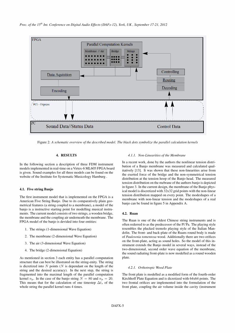
After a complete implementation of the models in MATLAB, thealgorithm is converted to VHDL and flashed onto a FPGA devel-opment board as described in section 1. The used hardware includea XILINX ML6O5 Virtex-6 development board for the calcula-tion of the implemented models and a standard Personal Computerwhere a C#-program acts as a user interface for controlling the pa-rameters of the physical model. The block diagram of the Banjomodel depicted in figure 2 gives a schematic overview of the corefunctionality.

3.4.1. Parallel Computation Kernels

To fully utilise the processing capabilities of the FPGA all core ele-ments of the FDM model are calculated in parallel. The calculationkernel of the 1-dimensional wave equation consists of 20 discretepoints that are calculated in parallel, in other words if a string isdiscretized with eighty points the kernel is executed four times.The other entities are modelled similarly. The parallel membranekernels have a 8x8 grid size, this means for a membrane discretizedwith 64x64 nodes, the parallel membrane kernels runs 8 times. Asimilar approach for 3-dimensional structures can be found in [32],[27].

3.4.2. Hardware Resources

The utilisation of hardware resources and clock speed on a FPGAdirectly depends on the complexity of the implemented design. Ona Virtex-6 FPGA one string including a bow model, as described in4, discretised with 80 points uses approximately 3% of the FPGAsresources and runs with a clock speed of≈ 80 Mhz. More complexdesigns, like a complete Violin geometry consume nearly 85% ofthe resources, but still run with a clock speed of ≈ 80 Mhz.

DAFX-4


Figure 2: A schematic overview of the described model. The black dots symbolize the parallel calculation kernels

4. RESULTS

In the following section a description of three FDM instrumentmodels implemented in real-time on a Virtex-6 ML605 FPGA boardis given. Sound examples for all three models can be found on thewebsite of the Institute for Systematic Musicology Hamburg .

4.1. Five string Banjo

The first instrument model that is implemented on the FPGA is aAmerican Five String Banjo. Due to its comparatively plain geo-metrical features (a string coupled to a membrane), a model of thebanjo is a instructive starting point for modelling musical instru-ments. The current model consists of two strings, a wooden bridge,the membrane and the coupling air underneath the membrane. TheFPGA model of the banjo is devided into four entities:

1. The strings (1-dimensional Wave Equation)

2. The membrane (2-dimensional Wave Equation)

3. The air (3-dimensional Wave Equation)

4. The bridge (2-dimensional Equation)

As mentioned in section 3 each entity has a parallel computationstructure that can best be illustrated on the string-enity. The stringis dicretized into N points (N is dependant on the length of thestring and the desired accuracy). In the next step, the string isfragmented into the maximal length of the parallel computationkernel np. In the case of the banjo string N = 80 and np = 20.This means that for the calculation of one timestep ∆ts of thewhole string the parallel kernel runs 4 times.

4.1.1. Non-Linearities of the Membrane

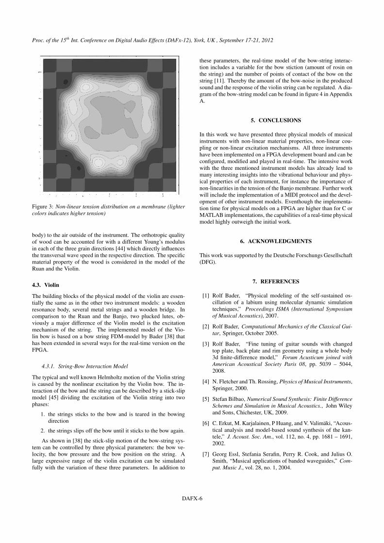
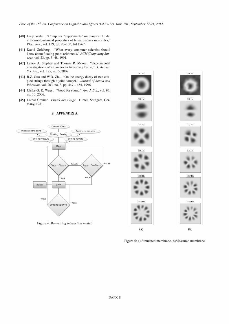
In a recent work, done by the authors the nonlinear tension distri-bution of a Banjo membrane was measured and calculated qual-itatively [13]. It was shown that these non-linearities arise fromthe exerted force of the bridge and the non-symmetrical tensiondistribution at the tension hoop of the Banjo head. The measuredtension distribution on the mebrane of the authors banjo is depictedin figure 3. In the current design, the membrane of the Banjo phys-ical model is discretized with 32x32 grid points with the non-lineartension distribution mapped on every point. The modeshapes of amembrane with non-linear tension and the modeshapes of a realbanjo can be found in figure 5 in Appendix A.

4.2. Ruan

The Ruan is one of the oldest Chinese string instruments and isoften rederred to as the predecessor of the Pi’Pa. The playing styleresembles the plucked tremolo playing style of the Italian Man-dolin. The front- and back-plate of the Ruans round body is madeof Paulownia tomentosa wood. Additionally there are two orificeson the front-plate, acting as sound holes. So the model of this in-strument extends the Banjo model in several ways, instead of thetwo-dimensional, second order wave equation of the membrane,the sound radiating front-plate is now modelled as a round woodenplate.

4.2.1. Orthotropic Wood Plate

The front plate is modelled as a modified form of the fourth-orderKirchhoff Plate Equation and is dicretized with 64x64 points. Thetwo frontal orifices are implemented into the formulation of thefront plate, coupling the air volume inside the cavity (instrument

DAFX-5

http://www.systmuwi.de/muwi_research_Physical_Modeling_of_Musical_Instruments.html


Figure 3: Non-linear tension distribution on a membrane (lightercolors indicates higher tension)

body) to the air outside of the instrument. The orthotropic qualityof wood can be accounted for with a different Young’s modulusin each of the three grain directions [44] which directly influencesthe transversal wave speed in the respective direction. The specificmaterial property of the wood is considered in the model of theRuan and the Violin.

4.3. Violin

The building blocks of the physical model of the violin are essen-tially the same as in the other two instrument models: a woodenresonance body, several metal strings and a wooden bridge. Incomparison to the Ruan and the Banjo, two plucked lutes, ob-viously a major difference of the Violin model is the excitationmechanism of the string. The implemented model of the Vio-lin bow is based on a bow string FDM-model by Bader [38] thathas been extended in several ways for the real-time version on theFPGA.

4.3.1. String-Bow Interaction Model

The typical and well known Helmholtz motion of the Violin stringis caused by the nonlinear excitation by the Violin bow. The in-teraction of the bow and the string can be described by a stick-slipmodel [45] dividing the excitation of the Violin string into twophases:

1. the strings sticks to the bow and is teared in the bowingdirection

2. the strings slips off the bow until it sticks to the bow again.

As shown in [38] the stick-slip motion of the bow-string sys-tem can be controlled by three physical parameters: the bow ve-locity, the bow pressure and the bow position on the string. Alarge expressive range of the violin excitation can be simulatedfully with the variation of these three parameters. In addition to

these parameters, the real-time model of the bow-string interac-tion includes a variable for the bow stiction (amount of rosin onthe string) and the number of points of contact of the bow on thestring [11]. Thereby the amount of the bow-noise in the producedsound and the response of the violin string can be regulated. A dia-gram of the bow-string model can be found in figure 4 in AppendixA.

5. CONCLUSIONS

In this work we have presented three physical models of musicalinstruments with non-linear material properties, non-linear cou-pling or non-linear excitation mechanisms. All three instrumentshave been implemented on a FPGA development board and can beconfigured, modified and played in real-time. The intensive workwith the three mentioned instrument models has already lead tomany interesting insights into the vibrational behaviour and phys-ical properties of each instrument, for instance the importance ofnon-linearities in the tension of the Banjo membrane. Further workwill include the implementation of a MIDI protocol and the devel-opment of other instrument models. Eventhough the implementa-tion time for physical models on a FPGA are higher than for C orMATLAB implementations, the capabilities of a real-time physicalmodel highly outweigh the initial work.

6. ACKNOWLEDGMENTS

This work was supported by the Deutsche Forschungs Gesellschaft(DFG).

7. REFERENCES

[1] Rolf Bader, “Physical modeling of the self-sustained os-cillation of a labium using molecular dynamic simulationtechniques,” Proceedings ISMA (International Symposiumof Musical Acoustics), 2007.

[2] Rolf Bader, Computational Mechanics of the Classical Gui-tar, Springer, October 2005.

[3] Rolf Bader, “Fine tuning of guitar sounds with changedtop plate, back plate and rim geometry using a whole body3d finite-difference model,” Forum Acusticum joined withAmerican Acoustical Society Paris 08, pp. 5039 – 5044,2008.

[4] N. Fletcher and Th. Rossing, Physics of Musical Instruments,Springer, 2000.

[5] Stefan Bilbao, Numerical Sound Synthesis: Finite DifferenceSchemes and Simulation in Musical Acoustics., John Wileyand Sons, Chichester, UK, 2009.

[6] C. Erkut, M. Karjalainen, P Huang, and V. Valimäki, “Acous-tical analysis and model-based sound synthesis of the kan-tele,” J. Acoust. Soc. Am., vol. 112, no. 4, pp. 1681 – 1691,2002.

[7] Georg Essl, Stefania Serafin, Perry R. Cook, and Julius O.Smith, “Musical applications of banded waveguides,” Com-put. Music J., vol. 28, no. 1, 2004.

DAFX-6


[8] F. Pfeifle and R. Bader, Musical Acoustics, Neurocognitionand Psychology of Music, chapter Real-Time Physical Mod-elling of a real Banjo geometry using FPGA hardware tech-nology., pp. 71–86, Rolf Bader, Frankfurt am Main, Ger-many, 2009.

[9] F. Pfeifle and R. Bader, “Real-time virtual banjo model andmeasurements using a microphone array.,” J. Acoust. Soc.Am., vol. 125, no. 4, pp. 2515 – 2515, 2009.

[10] F. Pfeifle and R. Bader, “Membrane modes and air reso-nances of the banjo using physical modeling and microphonearray measurements.,” J. Acoust. Soc. Am., vol. 127, no. 3,pp. 1870 – 1870, 2010.

[11] F. Pfeifle and R. Bader, “Real-time finite-difference string-bow interaction field programmable gate array (fpga) modelcoupled to a violin body,” J. Acoust. Soc. Am., vol. 130, no.4, pp. 2507 – 2507, 2011.

[12] F. Pfeifle and R. Bader, “Measurement and physical mod-elling of sound hole radiations of lutes,” J. Acoust. Soc. Am.,vol. 130, no. 4, pp. 2507 – 2507, 2011.

[13] F. Pfeifle and R. Bader, “Nonlinear coupling and tensioneffects in a real-time physical model of a banjo,” J. Acoust.Soc. Am., vol. 130, no. 4, pp. 2432 – 2432, 2011.

[14] F. Pfeifle and R. Bader, “Measurement and analysis of soundradiation patterns of the chinese ruan and the yueqin,” J.Acoust. Soc. Am., vol. 131, no. 4, pp. 3218 – 3218, 2012.

[15] K. Veggeberg and A. Zheng, “Real-time noise source iden-tification using programmable gate array(fpga) technology,”Proceedings of Meetings on Acoustics, vol. 5, 2009.

[16] C Hao and W. Ping, “The high speed implementation ofdirection-of-arrival estimation algorithmo,” InternationalConference on Communication, Circuits and Systems andWest Sino Expositions, vol. 2, pp. 922 – 925, 2002.

[17] B. Von Herzen, “Signal processing at 250 mhz using high-performance fpga’s,” IEEE Transactions onvery large scaleintegration (VLSI) Systems, vol. 6, no. 2, 1998.

[18] P. Chen, X. Tian, Y. Chen, and X. Yang, “Delay-sum beam-forming on fpga,” ICSP 2008 Proceedings, pp. 2542 – 2545,2008.

[19] Z. Wang, R. Jin, J. Geng, and Y. Fan, “Fpga implementationof downlink dbf calibration,” Antennas and Propagation So-ciety International Symposium, 2005.

[20] G. Martins, M. Barata, and L. Gomes, “Low cost method toreproduce sound with fpga,” IEEE International Symposiumon Industrial Electronics 2008, ISIE 2008, 2008.

[21] Uwe Meyer-Baese, Digital Signal Processing with FieldProgrammable Gate Arrays, Springer, Berlin, Heidelberg,2 edition, 2007.

[22] Juergen Reichardt and Bernd Schwarz, VHDL-Synthese:Entwurf digitaler Schaltungen und Systeme, Oldenbourg,Muenchen, 4 edition, 2009.

[23] A. Madanayake, L. Bruton, F. Comis, and C. Comis, “Fpgaarchitectures for real-time 2d/3d fir/iir plane wave filters,”Proceedings of the 2004 International Symposium on Cir-cuits and Systems ISCAS 2004, vol. 3, 2004.

[24] Kai Shuang, X. Yankai, J. Shan, and Z. Hongwu, “Con-verting analog controllers to digital controllers with fpga,”ICSP2008 Proceedings, 2008.

[25] O. Maslennikow and A Sergiyenko, “Mapping dsp algo-rithms into fpga,” Proceedings of the International Sympo-sium on Parallel Computing in Electrical Engineering, 2006.

[26] T. Brich, Novacek, K., and A. Khateb, “The digital signalprocessing using fpga,” ISSE 2006, 29th International SpringSeminar on Electronics Technology, pp. 322 – 324, 2006.

[27] E. Motuk, R. Woods, S Bilbao, and J. McAllistere, “De-sign methodology for real-time fpga-based sound synthesis,”IEEE Transactions on signal processing, vol. 55, no. 12,2007.

[28] Wang Chen, Panos Kosmas, Miriam Leeser, and Carey Rap-paport, “An fpga implementation of the two-dimensionalfinite-difference time-domain (fdtd) algorithm,” in Proceed-ings of the 2004 ACM/SIGDA 12th international symposiumon Field programmable gate arrays, New York, NY, USA,2004, pp. 213–222, ACM.

[29] K. L. Shlager and B. Schneider, “A selective survey of thefinite-diffrence time-domain literature,” IEEE Antennas andPropagation Magazine, vol. 37, no. No. IEEE 1995, 1995.

[30] R. Strzdoka and D. Göddeke, “Pipelined mixed precision al-gorithms on fpgas for fast and accurate pde solvers from lowprecision components,” 14th annual IEEE Symposium onField Programmable Custom Computing Machinges, 2006.

[31] M. Liu, W Kuehn, Z. Lu, and A. Jantsch, “System-on-an-fpga design for real-time particle track recognition in physicsexperiments,” 11th Euromicro Conference on Digital SystemDesign Architectures, Mthods and Tools, 2008.

[32] E. Motuk, R. Woods, and S Bilbao, “Implementation offinite-differece schemes for the wave equation on fpga,”IEEE International Acoustics Speech and Signal ProcessingICASSP 2005, vol. 3, 2005.

[33] J.A. Gibbons, D.M. Howard, and A.M. Tyrrell, “Fpga imple-mentation of 1d wave equation for real-time audio synthesis,”IEEE Proceedings, Computers and Digital Techniques, vol.152, no. 5, pp. 619 – 631, 2005.

[34] E. Becache, A. Chaigne, G. Derveaux, and P. Joly, “Fpgaparallel implementation of cmac type neural network withon chip learning,” IEEE, pp. 111 – 115, 2007.

[35] V. Subasri, K. Lavanya, and B. Umamaheswari, “Implemen-tation of digital pid controller in field programmable gate ar-ray(fpga),” Proceedings of India International Conferenceon Power Electronics 2006, 2006.

[36] J. D. Lis and C. T. Kowalski, “Parallel fixed point fpgaimplementation of sensorless induction motor torque con-trol,” 13th Power Electronics and Motion Control Confer-ence 2008. EPE-PEMC, 2008.

[37] Z. Zou, W. Hongyuan, and Y. Guowen, “An improved musicalgorithm implemented with high -speed parallel optimiza-tion for fpga,” 7th International Symposium on Antennas,Progpagation & EM Theory, ISAPE 2006, 2006.

[38] Rolf Bader, “Whole geometry finite-difference modeling ofthe violin,” Proceedings of the Forum Acusticum 2005, pp.629 – 634, 2005.

[39] Ernst Hairer, Christian Lubich, and Gerhard Wanner, “Geo-metric numerical integration illustrated by the störmer/verletmethod,” Acta Numerica, vol. 12, pp. 399–450, 2003.

DAFX-7


[40] Loup Verlet, “Computer "experiments" on classical fluids.i. thermodynamical properties of lennard-jones molecules,”Phys. Rev., vol. 159, pp. 98–103, Jul 1967.

[41] David Goldberg, “What every computer scientist shouldknow about floating-point arithmetic,” ACM Computing Sur-veys, vol. 23, pp. 5–48, 1991.

[42] Laurie A. Stephey and Thomas R. Moore, “Experimentalinvestigations of an american five-string banjo,” J. Acoust.Soc Am., vol. 125, no. 5, 2008.

[43] B.Z. Guo and W.D. Zhu, “On the energy decay of two cou-pled strings through a joint damper,” Journal of Sound andVibration, vol. 203, no. 3, pp. 447 – 455, 1996.

[44] Ulrike G. K. Wegst, “Wood for sound,” Am. J. Bot., vol. 93,no. 10, 2006.

[45] Lothar Cremer, Physik der Geige, Hirzel, Stuttgart, Ger-many, 1981.

8. APPENDIX A

Figure 4: Bow-string interaction model.

(a) (b)

Figure 5: a) Simulated membrane. b)Measured membrane

DAFX-8

Documents

Real-time Finite Difference Physical Models of Musical