Studies on dust-plasma interaction in Saturn’s inner ...psg/doc2014/shotaro_D/sakai_D...Final examination for PhD, 4 February 2014 Studies on dust-plasma interaction in Saturn’s

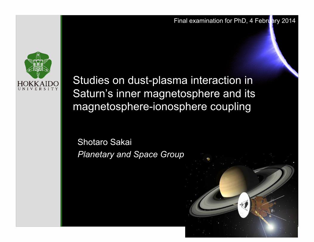
Final examination for PhD, 4 February 2014

Studies on dust-plasma interaction in Saturn’s inner magnetosphere and its magnetosphere-ionosphere coupling

Shotaro Sakai Planetary and Space Group

Outline of my thesis Structure of my doctoral thesis 1.  General Introduction 2.  Enceladus plume observed by Cassini RPWS/LP 3.  Modeling of the inner magnetosphere 4.  Modeling of the ionosphere 5.  Magnetosphere-ionosphere coupling 6.  Summary

Outline of my thesis Structure of my doctoral thesis 1.  General Introduction 2.  Enceladus plume observed by Cassini RPWS/LP 3.  Modeling of the inner magnetosphere 4.  Modeling of the ionosphere 5.  Magnetosphere-ionosphere coupling 6.  Summary

Introduction

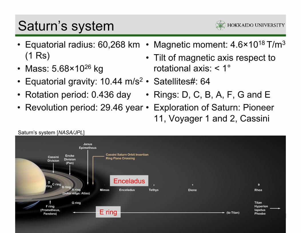
Saturn’s system

Saturn’s system [NASA/JPL]

E ring

Enceladus

•  Equatorial radius: 60,268 km (1 Rs)

•  Mass: 5.68×1026 kg •  Equatorial gravity: 10.44 m/s2 •  Rotation period: 0.436 day •  Revolution period: 29.46 year

•  Magnetic moment: 4.6×1018 T/m3 •  Tilt of magnetic axis respect to

rotational axis: < 1° •  Satellites#: 64 •  Rings: D, C, B, A, F, G and E •  Exploration of Saturn: Pioneer

11, Voyager 1 and 2, Cassini

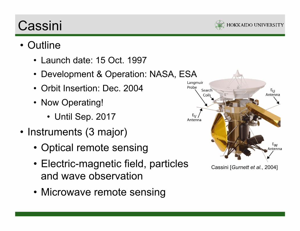
Cassini •  Outline

•  Launch date: 15 Oct. 1997 •  Development & Operation: NASA, ESA •  Orbit Insertion: Dec. 2004 •  Now Operating!

•  Until Sep. 2017

•  Instruments (3 major) •  Optical remote sensing •  Electric-magnetic field, particles

and wave observation •  Microwave remote sensing

Cassini [Gurnett et al., 2004]

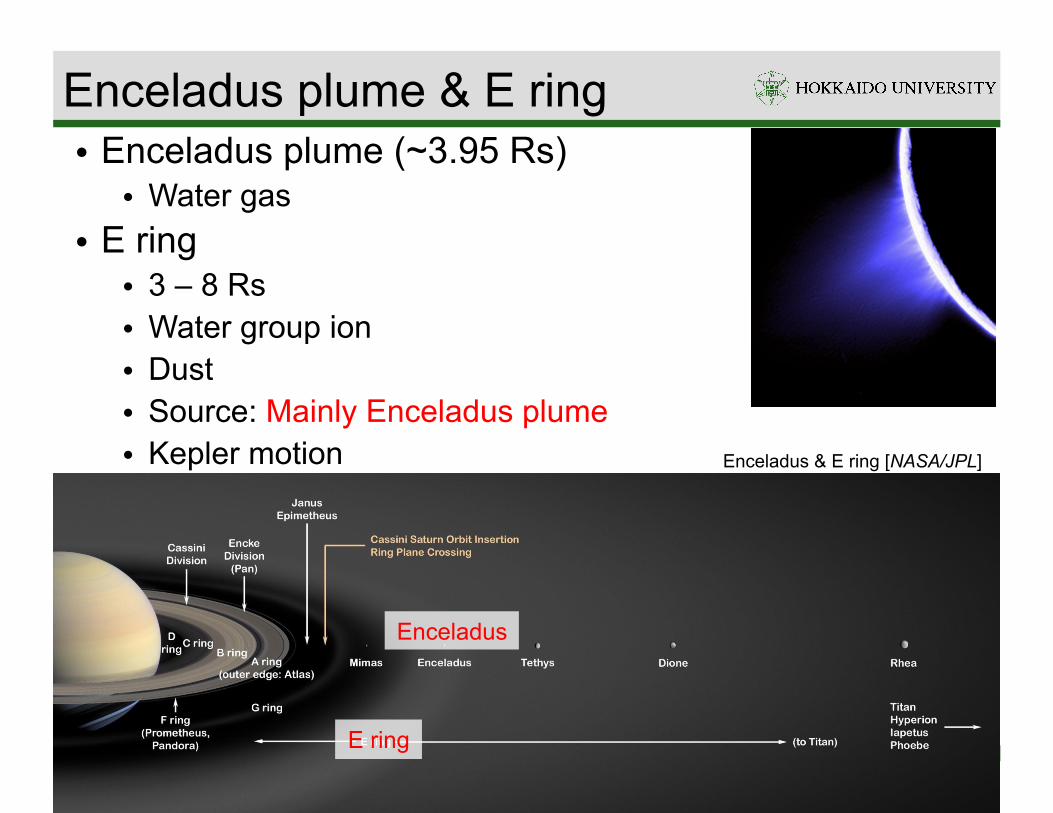
Enceladus plume & E ring • Enceladus plume (~3.95 Rs) •  Water gas

• E ring •  3 – 8 Rs •  Water group ion •  Dust •  Source: Mainly Enceladus plume •  Kepler motion Enceladus & E ring [NASA/JPL]

E ring

Enceladus

0

100

200

300

I prob

e [nA]

Cassini LP 2012.04.14. 13:59:11.8 UT (E18)

10−10

10−8

I prob

e [A]

−30 −20 −10 0 10 20 30

0

10

20

30

dIpr

obe/d

U [n

A/V]

Ubias [V]

Cassini Langmuir Probe (LP) •  Length: 1.5 m, Diameter: 50 mm •  Titanium •  LP measures currents by changing the probe voltage

from -32 to 32 V.

Cassini & Cassini LP [Gurnett et al., 2004]

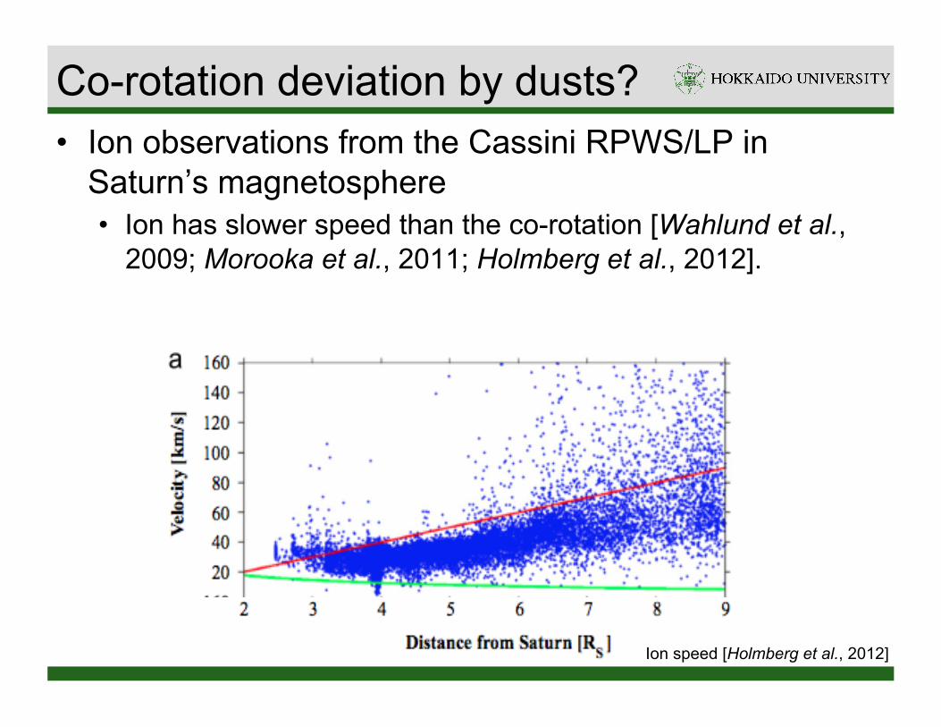
Co-rotation deviation by dusts?

Ion speed [Holmberg et al., 2012]

•  Ion observations from the Cassini RPWS/LP in Saturn’s magnetosphere •  Ion has slower speed than the co-rotation [Wahlund et al.,

2009; Morooka et al., 2011; Holmberg et al., 2012].

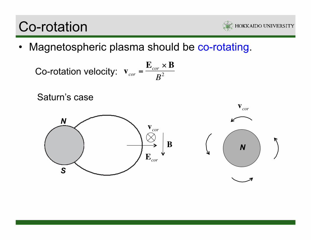
Co-rotation •  Magnetospheric plasma should be co-rotating.

Co-rotation velocity:

€

vcor =Ecor × BB2

€

Ecor

€

B €

vcorN

S

N

Saturn’s case

€

vcor


Ion speed [Holmberg et al., 2012]

•  Ion observations from the Cassini RPWS/LP in Saturn’s magnetosphere •  Ion has slower speed than the co-rotation [Wahlund et al.,

2009; Morooka et al., 2011; Holmberg et al., 2012]. •  Do dusts affect the ion velocities in the inner

magnetosphere?

•  Investigation of dust-plasma interaction and magnetosphere-ionosphere coupling in the Saturn’s inner magnetosphere

• Understanding of generation process for magnetospheric current, electric field and ion-dust collision

• Understanding of relationship of ionospheric conductivity with the magnetospheric ion speed

Purpose of this thesis

•  Density •  Ne/Ni < 0.01 at 1.3 RE

~ 0.7 at 11 RE

Plasma in the plume

•  Ion speed •  Vi ~ VKepler

Ion density and speed in plume [Sakai et al., in prep.]

−6 −3 0 3 6

−12

−9

−6

−3

0

X, Distance from Enceladus [RE]

Z, D

istan

ce fr

om E

ncela

dus [

R E]

Ion density [cm−3]

a

40

60

80

100

120

140

−6 −3 0 3 6

−12

−9

−6

−3

0


Ion velocity [km s−1]

b

5

10

15

20

25

30

Charged dust in the plume •  Dust density ~1.3 RE Ndmax > 10 cm-3 ~7 RE Ndmax ~ 1 cm-3

~11 RE Ndmax ~ 0.1 cm-3

−6 −3 0 3 6

−12

−9

−6

−3

0


Z, D

istan

ce fr

om E

ncela

dus [

R E]


a

40

60

80

100

120

140

−6 −3 0 3 6

−12

−9

−6

−3

0


Dust density (log(Nd))[cm−3]

b

−1.5

−1

−0.5

0

0.5

1

1.5

−6 −3 0 3 6

−12

−9

−6

−3

0


Z, D

istan

ce fr

om E

ncela

dus [

R E]


a

40

60

80

100

120

140

−6 −3 0 3 6

−12

−9

−6

−3

0


Dust density (log(Nd))[cm−3]

b

−1.5

−1

−0.5

0

0.5

1

1.5

Modeling of the inner magnetosphere

Model •  Multi-fluid model (H+, H2O+, dust, e-) •  1 dimension (radial direction), 2 RS to 10 RS

•  Vr, Vφ are calculated.

2 Rs to 10 Rs, one dimension

2 Rs 10 Rs

N

S

•  Initial condition •  Ion speed: Co-rotation speed; Dust speed: Keplerian speed

•  Boundary condition •  Inner boundary

•  Ion speed: Co-rotation speed; Dust speed: Keplerian speed •  Open outer boundary

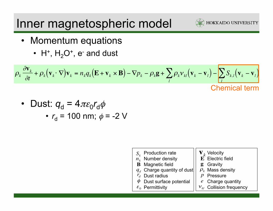
•  Momentum equations •  H+, H2O+, e- and dust

•  Dust: qd = 4πε0rdφ •  rd = 100 nm; φ = -2 V

Inner magnetospheric model

€

ρk∂vk∂t

+ ρk vk ⋅ ∇( )vk = nkqk E + vk × B( ) −∇pk − ρkg + ρkν kl vk − vl( )l∑ − Sk,l vk − vl( )

l∑

Velocity Electric field Gravity Mass density Pressure Charge quantity Collision frequency €

vk

€

E

€

g

€

ρk

€

p

€

e

€

νkl

Production rate Number density Magnetic field Charge quantity of dust Dust radius Dust surface potential Permittivity

€

Sk

€

nk

€

B

€

qd

€

rd

€

φ

€

ε 0

Chemical term

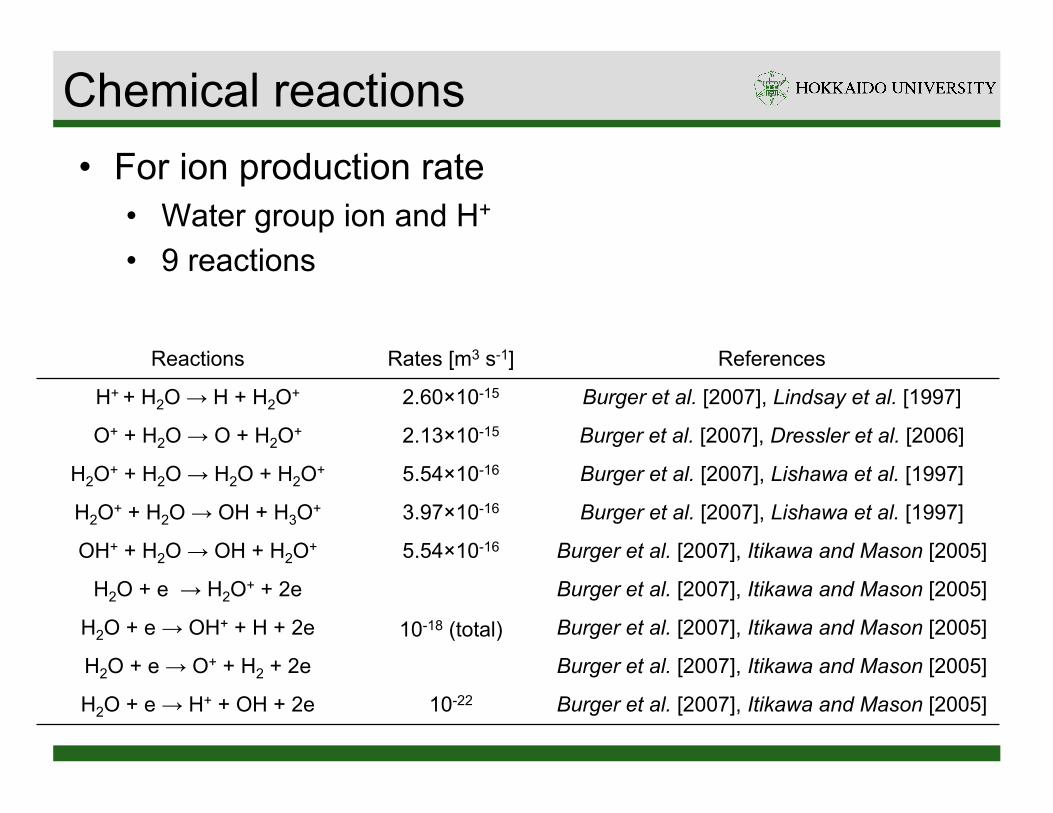
Chemical reactions •  For ion production rate

•  Water group ion and H+ •  9 reactions

Reactions Rates [m3 s-1] References

H+ + H2O → H + H2O+ 2.60×10-15 Burger et al. [2007], Lindsay et al. [1997]

O+ + H2O → O + H2O+ 2.13×10-15 Burger et al. [2007], Dressler et al. [2006]

H2O+ + H2O → H2O + H2O+ 5.54×10-16 Burger et al. [2007], Lishawa et al. [1997]

H2O+ + H2O → OH + H3O+ 3.97×10-16 Burger et al. [2007], Lishawa et al. [1997]

OH+ + H2O → OH + H2O+ 5.54×10-16 Burger et al. [2007], Itikawa and Mason [2005]

H2O + e → H2O+ + 2e

10-18 (total)Burger et al. [2007], Itikawa and Mason [2005]

H2O + e → OH+ + H + 2e Burger et al. [2007], Itikawa and Mason [2005]

H2O + e → O+ + H2 + 2e Burger et al. [2007], Itikawa and Mason [2005]

H2O + e → H+ + OH + 2e 10-22 Burger et al. [2007], Itikawa and Mason [2005]

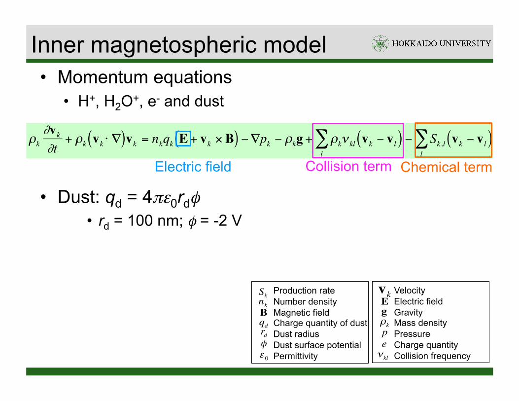
•  Momentum equations •  H+, H2O+, e- and dust

•  Dust: qd = 4πε0rdφ •  rd = 100 nm; φ = -2 V

Inner magnetospheric model

€

ρk∂vk∂t


l∑

Velocity Electric field Gravity Mass density Pressure Charge quantity Collision frequency €

vk

€

E

€

g

€

ρk

€

p

€

e

€

νkl

Collision termElectric field

Production rate Number density Magnetic field Charge quantity of dust Dust radius Dust surface potential Permittivity

€

Sk

€

nk

€

B

€

qd

€

rd

€

φ

€

ε 0

Chemical term

•  M-I coupling for deriving electric field, E

•  Ionospheric conductivity Σi: 1 S

Electric field

jD

Σi(Ecor - E)current

D

current

€

Σi Ecor −E( ) = jDj = enivi − eneve − qdndvd

€

E = Ecor −jDΣi

↓ ↓ ↓Thickness of dust distribution

Current density Co-rotational Electric field Ionospheric conductivity Thickness of dust Thermal velocity

€

j

€

Ecor

€

Σi

€

D

€

vthk

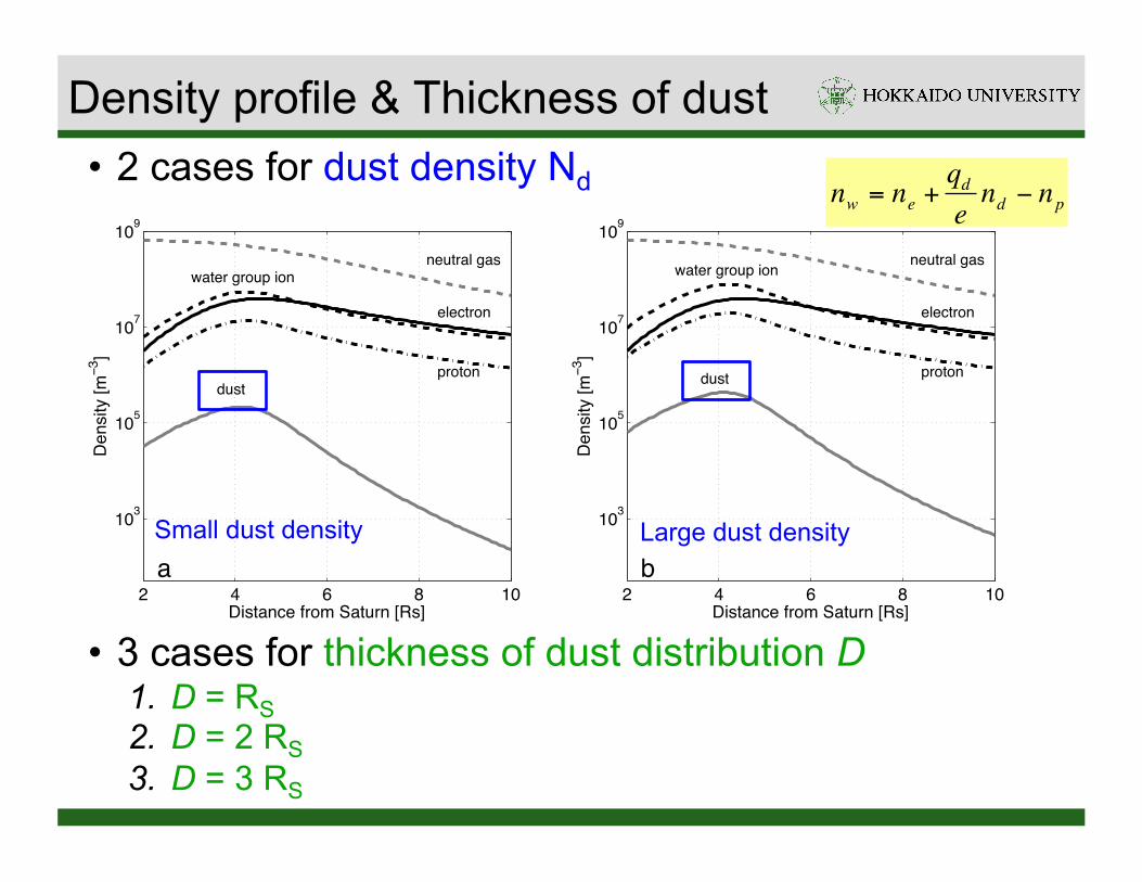
Density profile & Thickness of dust

•  3 cases for thickness of dust distribution D 1.  D = RS 2.  D = 2 RS 3.  D = 3 RS

•  2 cases for dust density Nd

2 4 6 8 10

103

105

107

109

Distance from Saturn [Rs]

Den

sity

[m−3

]

a

neutral gaswater group ion

electron

protondust

2 4 6 8 10

103

105

107

109

Distance from Saturn [Rs]D

ensi

ty [m

−3]

b


electron

protondust

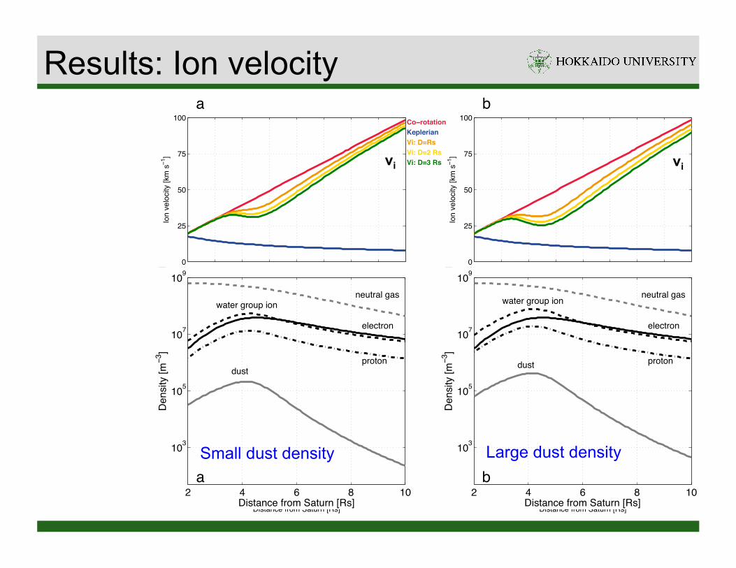
Small dust density Large dust density

€

nw = ne +qdend − np

0

25

50

75

100a

Ion

velo

city

[km

s−1

]

Co−rotationKeplerianVi: D=RsVi: D=2 RsVi: D=3 Rs

j: D=Rsj: D=2 Rsj: D=3 Rs

E: D=RsE: D=2 RsE: D=3 Rs

Gyro freq.i

wd: D=Rs

iwd

: D=2 Rsi

wd: D=3 Rs

10−13

10−12

10−11

10−10

Cur

rent

den

sity

[A m

−2]

10−5

10−4

10−3

10−2

Elec

tric

field

[V m

−1]

2 3 4 5 6 7 8 9 1010−8

10−4

100

Freq

uenc

y [s−1

]


0

25

50

75

100b

Ion

velo

city

[km

s−1

]

10−13

10−12

10−11

10−10

Cur

rent

den

sity

[A m

−2]

10−5

10−4

10−3

10−2

Elec

tric

field

[V m

−1]

2 3 4 5 6 7 8 9 1010−8

10−4

100

Freq

uenc

y [s−1

]


j j

Em Em

ν, Ω ν, Ω

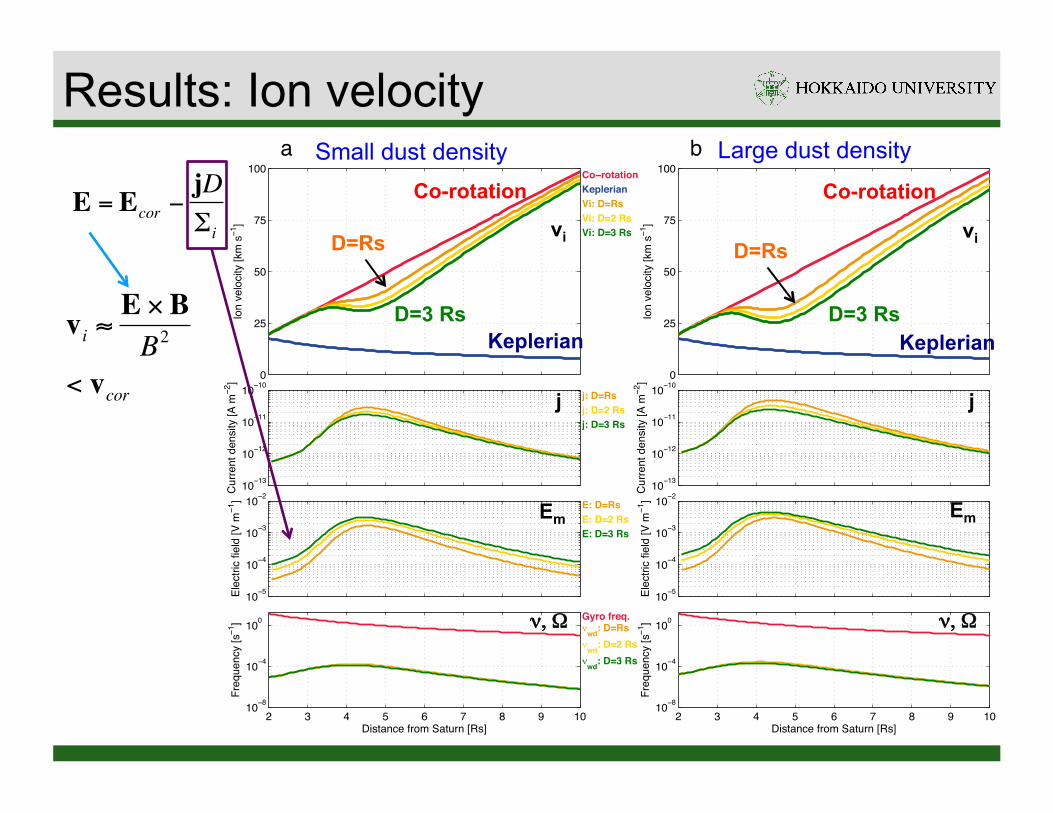
vi vi

Results: Ion velocity

2 4 6 8 10

103

105

107

109


Den

sity

[m−3

]

a


electron

protondust

2 4 6 8 10

103

105

107

109


Den

sity

[m−3

]

b


electron

protondust


0

25

50

75

100a

Ion

velo

city

[km

s−1

]

Co−rotationKeplerianVi: D=RsVi: D=2 RsVi: D=3 Rs

j: D=Rsj: D=2 Rsj: D=3 Rs

E: D=RsE: D=2 RsE: D=3 Rs

Gyro freq.i

wd: D=Rs

iwd

: D=2 Rsi

wd: D=3 Rs

10−13

10−12

10−11

10−10

Cur

rent

den

sity

[A m

−2]

10−5

10−4

10−3

10−2

Elec

tric

field

[V m

−1]

2 3 4 5 6 7 8 9 1010−8

10−4

100

Freq

uenc

y [s−1

]


0

25

50

75

100b

Ion

velo

city

[km

s−1

]

10−13

10−12

10−11

10−10

Cur

rent

den

sity

[A m

−2]

10−5

10−4

10−3

10−2

Elec

tric

field

[V m

−1]

2 3 4 5 6 7 8 9 1010−8

10−4

100

Freq

uenc

y [s−1

]


j j

Em Em

ν, Ω ν, Ω

vi viD=Rs

D=3 Rs

D=Rs

D=3 Rs

Co-rotation Co-rotation

Keplerian Keplerian

Results: Ion velocity Small dust density Large dust density

€

E = Ecor −jDΣi

€

vi ≈E × BB2

< vcor

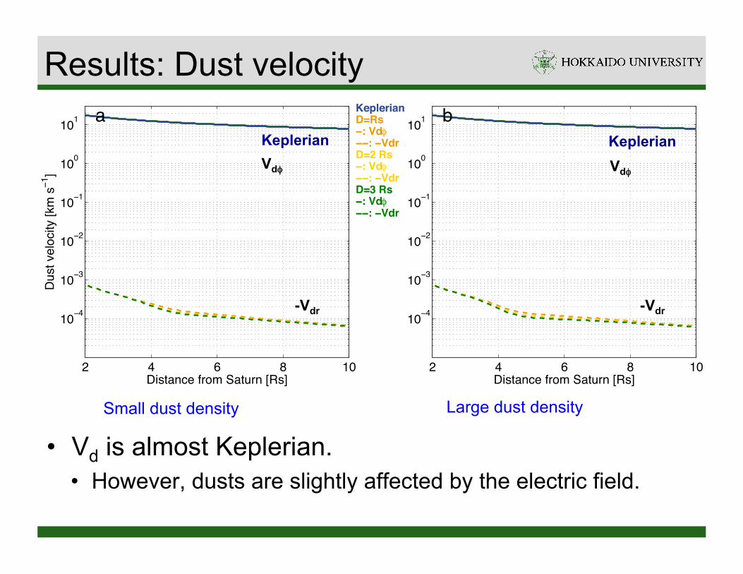
Results: Dust velocity


2 4 6 8 10

10−4

10−3

10−2

10−1

100

101 a


Dus

t vel

ocity

[km

s−1

]

KeplerianD=Rs−: Vdq−−: −VdrD=2 Rs−: Vdq−−: −VdrD=3 Rs−: Vdq−−: −Vdr

2 4 6 8 10

10−4

10−3

10−2

10−1

100

101 b


Keplerian KeplerianVdφ Vdφ

-Vdr-Vdr

•  Vd is almost Keplerian. •  However, dusts are slightly affected by the electric field.

Comparison with LP observation

•  Consistent with observations in Nd > ~105 m-3 and/or D > 1 RS.


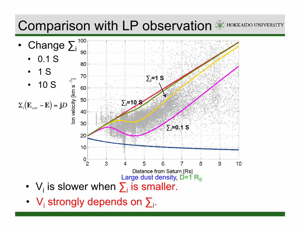
∑i=0.1 S

∑i=1 S

∑i=10 S

Comparison with LP observation

•  Vi is slower when ∑i is smaller. •  Vi strongly depends on ∑i.

Large dust density, D=1 RS

•  Change ∑i •  0.1 S •  1 S •  10 S

€

Σi Ecor −E( ) = jD

Summary •  Co-rotation lag

•  Dust-plasma interaction •  The dust–plasma interaction is significant when D is large

and/or Nd is high. •  Nd max > ~105 m-3 •  D > 1 RS

•  The inner magnetospheric total current along a magnetic field line weakens E.

•  Vd is almost the Keplerian. •  However, dusts are slightly affected by this interaction.

•  Ionosphere and magnetosphere are strongly coupled. •  Vi depends on ∑i.

Modeling of the ionosphere & Magnetosphere-ionosphere coupling

•  Ionospheric Pedersen conductivity •  E depends on the conductivity.


€

σp =ν i

ν in2 +ω ci

2nie

2

mi

+ν e

ν en2 +ω ce

2nee

2

mei∑

€

Σi = σpdsz1

z2∫

€

ρk∂vk∂t


l∑

Electric field

€


Pedersen conductivity

•  However, it is one of the open questions. •  ~0.1-100 S [Connerney et al., 1983; Cheng and Waite, 1988] •  ~0.02 S [Saur et al., 2004] •  1--10 S [Cowley et al., 2004; Moore et al., 2010]

• We find the ionospheric Ni for deriving ∑i.

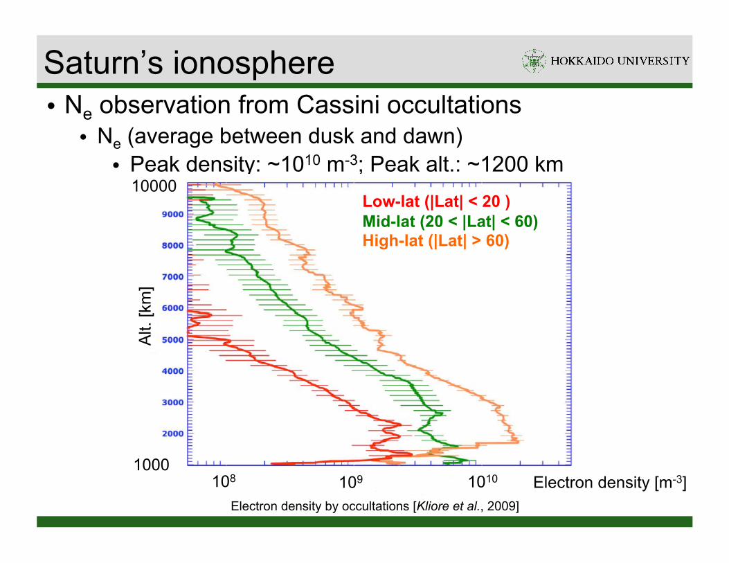
• Ne observation from Cassini occultations •  Ne (average between dusk and dawn) •  Peak density: ~1010 m-3; Peak alt.: ~1200 km

Electron density by occultations [Kliore et al., 2009]

Saturn’s ionosphere

Low-lat (|Lat| < 20 ) Mid-lat (20 < |Lat| < 60) High-lat (|Lat| > 60)

108 109 10101000

10000

Alt.

[km

]

Electron density [m-3]

• Model [Moore et al. 2008] •  Ne

•  Average peak density: ~1010 m-3

•  Peak alt.: ~1200 km •  Te

•  Max: 500 K •  Alt.: > 1500 km

• But only below ~3000 km •  How is the magnetospheric

influence?

Plasma density and temperature by modeling [Moore et al., 2008]

Saturn’s ionosphere

•  Construction of an ionospheric model including the inner magnetosphere.

•  Estimation of the ionospheric Pedersen conductivity from plasma density in the Saturn’s ionosphere

•  Investigation of the influence of magnetosphere to ionosphere

Purpose

•  Primitive equations •  Ion

•  Electron

3 dimensional ionospheric model Field-aligned Velocity Electric field Magnetic flux cross-section Gravity and CF Temperature Heating rate Diffusion coefficient €

v||

€

E||

€

g

€

κ€

A

€

T

€

Q

€

∂ρi∂t

+1A∂ Aρivi,||( )

∂s= Si − Li

ρi∂vi,||∂t

+ ρivi,||∂vi,||∂s

= nieE || −∂pi∂s

− ρig − ρiν ik vi,|| − vk,||( )k∑

Ti = Te

€

ne = nii∑

E|| = −1ene

∂pe∂s

∂Te∂t

−231A∂∂s

Aκe∂Te∂s

⎛

⎝ ⎜

⎞

⎠ ⎟ =QEUV +Qcoll +Qjoule +Qph,ionos +Qph,mag

Density:

Momentum:

Temperature:

Density:

Momentum:

Temperature:

Ni (H+, H2+, H3

+, He+, H2O+ and H3O+),

Vi (H+, H2+, H3

+, He+, H2O+ and H3O+),

Te, Ti

Model •  Dipole coordinate system

N

S

+ Increasing the number of magnetic field line → 2 dimensions

+ Time evolution → 3 dimensions

☓

•  Along the magnetic field line → 1 dimension


•  Electron

3 dimensional ionospheric model Field-aligned Velocity Electric field Magnetic flux cross-section Gravity and CF Temperature Heating rate Diffusion coefficient €

v||

€

E||

€

g

€

κ€

A

€

T

€

Q

€

∂ρi∂t

+1A∂ Aρivi,||( )

∂s= Si − Li

ρi∂vi,||∂t



− ρig − ρiν ik vi,|| − vk,||( )k∑

Ti = Te

€

ne = nii∑

E|| = −1ene

∂pe∂s

∂Te∂t

−231A∂∂s

Aκe∂Te∂s

⎛

⎝ ⎜

⎞


Density:

Momentum:

Temperature:

Density:

Momentum:

Temperature:

Source and Loss rate

Ni (H+, H2+, H3

+, He+, H2O+ and H3O+),

Vi (H+, H2+, H3

+, He+, H2O+ and H3O+),

Te, Ti

•  Chemical reactions of 6 ion components •  H+, H2

+, H3+, He+, H2O+ and H3O+

•  29 reactions

Source & Loss

4.3 Atmospheric Model 47Table 4.1: Photoionization reactions, ion recombination and charge exchange reactions

Chemical reaction Rate coefficiants ReferencesH + hν → H+ + e− Moses and Bass [2000]H2 + hν → H+ + H + e− Moses and Bass [2000]H2 + hν → H+

2 + e− Moses and Bass [2000]He + hν → He+ + e− Moses and Bass [2000]H2O + hν → H+ + OH + e− Moses and Bass [2000]H2O + hν → H2O+ + e− Moses and Bass [2000]H+ + e− → H 1.9 × 10−16T−0.7

e Moses and Bass [2000];Kim and Fox [1994]

H+2 + e− → H + H 2.3 × 10−12T−0.4


H+3 + e− → H2 + H 7.6 × 10−13T−0.5


H+3 + e− → 3H 9.7 × 10−13T−0.5


He+ + e− → He 1.9 × 10−16T−0.7e Moses and Bass [2000];

Kim and Fox [1994]H2O+ + e− → O + H2 3.5 × 10−12T−0.5

e Moses and Bass [2000];Miller et al. [1997]

H2O+ + e− → OH + H 2.8 × 10−12T−0.5e Moses and Bass [2000];

Miller et al. [1997]H3O+ + e− → H2O + H 6.1 × 10−12T−0.5


H3O+ + e− → OH + 2H 1.1 × 10−11T−0.5e Moses and Bass [2000];

Miller et al. [1997]H+ + H2 → H+

2 + H see text Moses and Bass [2000]H+ + H2 + M → H+

3 + M 3.2 × 10−41 Moses and Bass [2000];Kim and Fox [1994]

H+ + H2O → H2O+ + H 8.2 × 10−15 Moses and Bass [2000];Anicich [1993]

H+2 + H → H+ + H2 6.4 × 10−16 Moses and Bass [2000];

Anicich [1993]H+

2 + H2 → H+3 + H 2.0 × 10−15 Moses and Bass [2000];

Kim and Fox [1994]H+

2 + H2O → H2O+ + H2 3.9 × 10−15 Moses and Bass [2000];Anicich [1993]

H+2 + H2O → H3O+ + H 3.4 × 10−15 Moses and Bass [2000];

Anicich [1993]H+


He+ + H2 → H+ + H + He 8.8 × 10−20 Matcheva et al. [2001];Perry [1999]

He+ + H2 → H+2 + He 9.4 × 10−21 Moses and Bass [2000];

Kim and Fox [1994]He+ + H2O → H+ + OH + He 1.9 × 10−16 Moses and Bass [2000];

Anicich [1993]He+ + H2O → H2O+ + He 5.5 × 10−17 Moses and Bass [2000];

Anicich [1993]H2O+ + H2 → H3O+ + H 7.6 × 10−16 Moses and Bass [2000];

Anicich [1993]H2O+ + H2O → H3O+ + OH 1.9 × 10−15 Moses and Bass [2000];

Anicich [1993]XX January 2014(Shotaro SAKAI)

4.3 Atmospheric Model 47Table 4.1: Photoionization reactions, ion recombination and charge exchange reactions

Chemical reaction Rate coefficiants ReferencesH + hν → H+ + e− Moses and Bass [2000]H2 + hν → H+ + H + e− Moses and Bass [2000]H2 + hν → H+

2 + e− Moses and Bass [2000]He + hν → He+ + e− Moses and Bass [2000]H2O + hν → H+ + OH + e− Moses and Bass [2000]H2O + hν → H2O+ + e− Moses and Bass [2000]H+ + e− → H 1.9 × 10−16T−0.7


H+2 + e− → H + H 2.3 × 10−12T−0.4


H+3 + e− → H2 + H 7.6 × 10−13T−0.5


H+3 + e− → 3H 9.7 × 10−13T−0.5


He+ + e− → He 1.9 × 10−16T−0.7e Moses and Bass [2000];

Kim and Fox [1994]H2O+ + e− → O + H2 3.5 × 10−12T−0.5


H2O+ + e− → OH + H 2.8 × 10−12T−0.5e Moses and Bass [2000];

Miller et al. [1997]H3O+ + e− → H2O + H 6.1 × 10−12T−0.5


H3O+ + e− → OH + 2H 1.1 × 10−11T−0.5e Moses and Bass [2000];

Miller et al. [1997]H+ + H2 → H+

2 + H see text Moses and Bass [2000]H+ + H2 + M → H+

3 + M 3.2 × 10−41 Moses and Bass [2000];Kim and Fox [1994]

H+ + H2O → H2O+ + H 8.2 × 10−15 Moses and Bass [2000];Anicich [1993]

H+2 + H → H+ + H2 6.4 × 10−16 Moses and Bass [2000];

Anicich [1993]H+

2 + H2 → H+3 + H 2.0 × 10−15 Moses and Bass [2000];

Kim and Fox [1994]H+


H+2 + H2O → H3O+ + H 3.4 × 10−15 Moses and Bass [2000];

Anicich [1993]H+


He+ + H2 → H+ + H + He 8.8 × 10−20 Matcheva et al. [2001];Perry [1999]

He+ + H2 → H+2 + He 9.4 × 10−21 Moses and Bass [2000];

Kim and Fox [1994]He+ + H2O → H+ + OH + He 1.9 × 10−16 Moses and Bass [2000];

Anicich [1993]He+ + H2O → H2O+ + He 5.5 × 10−17 Moses and Bass [2000];

Anicich [1993]H2O+ + H2 → H3O+ + H 7.6 × 10−16 Moses and Bass [2000];

Anicich [1993]H2O+ + H2O → H3O+ + OH 1.9 × 10−15 Moses and Bass [2000];

Anicich [1993]XX January 2014(Shotaro SAKAI)


•  Electron

Field-aligned Velocity Electric field Magnetic flux cross-section Gravity and CF Temperature Heating rate Diffusion coefficient €

v||

€

E||

€

g

€

κ€

A

€

T

€

Q

€

∂ρi∂t

+1A∂ Aρivi,||( )

∂s= Si − Li

ρi∂vi,||∂t



− ρig − ρiν ik vi,|| − vk,||( )k∑

Ti = Te

€

ne = nii∑

E|| = −1ene

∂pe∂s

∂Te∂t

−231A∂∂s

Aκe∂Te∂s

⎛

⎝ ⎜

⎞


Density:

Momentum:

Temperature:

Density:

Momentum:

Temperature:

Source and Loss rate

Heating rateHeat flow, QHF

EUV, collision, Joule heating, photoelectron

3 dimensional ionospheric model

Ni (H+, H2+, H3

+, He+, H2O+ and H3O+),

Vi (H+, H2+, H3

+, He+, H2O+ and H3O+),

Te, Ti

107 1011 1015 1019 10230

1000

2000

3000

4000

5000

6000

7000

8000

9000

Density [m−3]

Altit

ude

[km

]Neutral density [m−3]

H

H2

He

H2O

a

200 400 600Temperature [K]

Neutral temperature [K]

Tnb

Background neutral atmosphere

104 106 108 1010

1000

2000

3000

4000

5000

6000

7000

8000

9000

10000

Density [m−3]

Altit

ude

[km

]

Plasma density

H+

H2+

H3+

He+

HXO+

e−

a

−10 0 10 20Velocity [km/s]

Ion velocity

H+

H2+

H3+

He+

HXO+

b

10−17 10−13 10−9 10−5

Conductivity [S/m]


m pc

•  Ni •  H3

+ is dominant. Max: ~1010 m-3

•  σi •  Maximum around 1000 km

•  Vi •  Upward velocity

•  Light component •  Downward velocity

•  Heavy component

Ni, Vi, σp (L=5, LT=12)

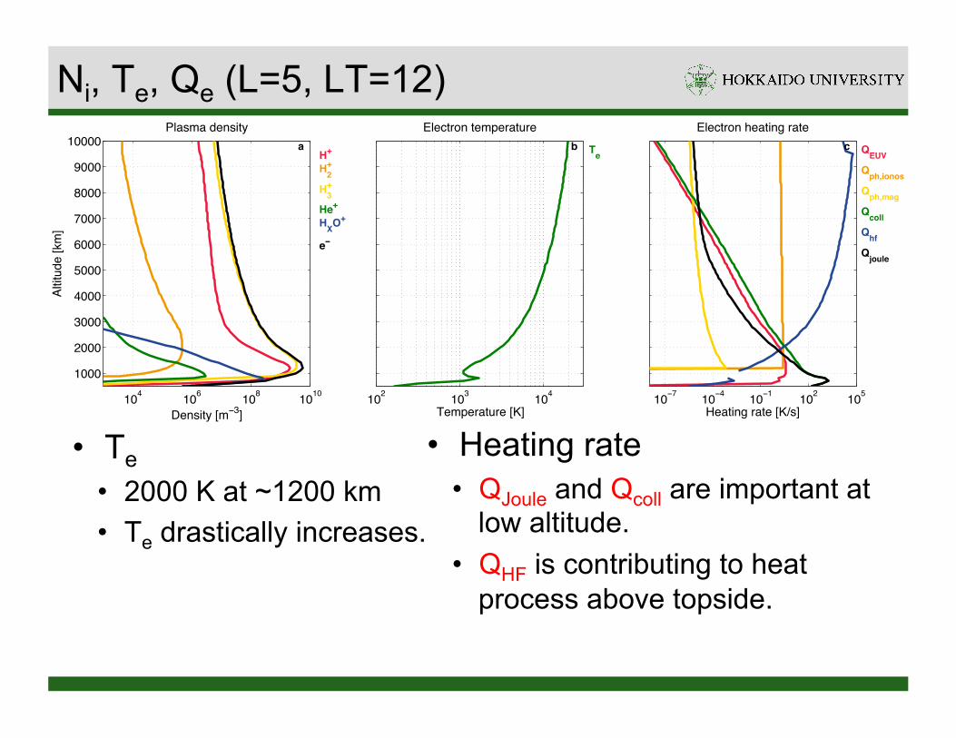
•  Te •  2000 K at ~1200 km •  Te drastically increases.

•  Heating rate •  QJoule and Qcoll are important at

low altitude. •  QHF is contributing to heat

process above topside.

Ni, Te, Qe (L=5, LT=12)

104 106 108 1010

1000

2000

3000

4000

5000

6000

7000

8000

9000

10000

Density [m−3]

Altit

ude

[km

]

Plasma density

H+

H2+

H3+

He+

HXO+

e−

a

102 103 104

Temperature [K]

Electron temperature

Teb

10−7 10−4 10−1 102 105

Heating rate [K/s]

Electron heating rate

QEUVQph,ionosQph,magQcollQhfQjoule

c

102 103 104

1000

2000

3000

4000

5000

6000

7000

8000

9000

10000

Temperature [K]

Altit

ude

[km

]

Electron temperature (L=5)a− QJoule & QHF

− − Without QHF

− Without QJoule & QHF

Joule heating & Heat flow

•  Te doesn’t have a peak without QJoule. •  Te decreases at topside without QHF.

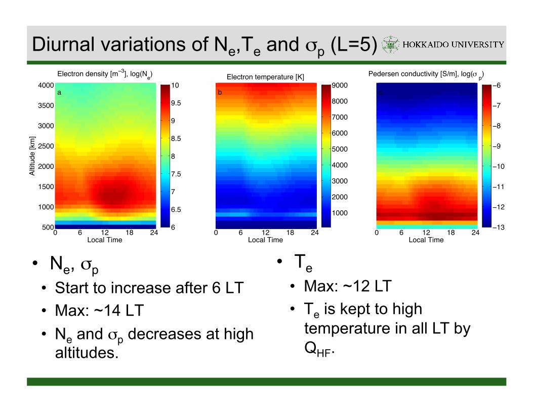
•  Ne, σp •  Start to increase after 6 LT •  Max: ~14 LT •  Ne and σp decreases at high

altitudes.

•  Te •  Max: ~12 LT •  Te is kept to high

temperature in all LT by QHF.

Diurnal variations of Ne,Te and σp (L=5)

0 6 12 18 24500

1000

1500

2000

2500

3000

3500

4000

Local Time

Altit

ude

[km

]

Electron density [m−3], log(Ne)

a

6

6.5

7

7.5

8

8.5

9

9.5

10

0 6 12 18 24Local Time

Electron temperature [K]

b

1000

2000

3000

4000

5000

6000

7000

8000

9000

0 6 12 18 24Local Time

Pedersen conductivity [S/m], log(m p)

c

−13

−12

−11

−10

−9

−8

−7

−6

2 3 4 5 6 7 8 90

0.2

0.4

0.6

0.8

1

1.2

1.4

1.6

1.8

2

Distance from Saturn [RS]

Con

duct

ivity

[S]

Pedersen Conductivity

Day

Dusk

Night

Dawn

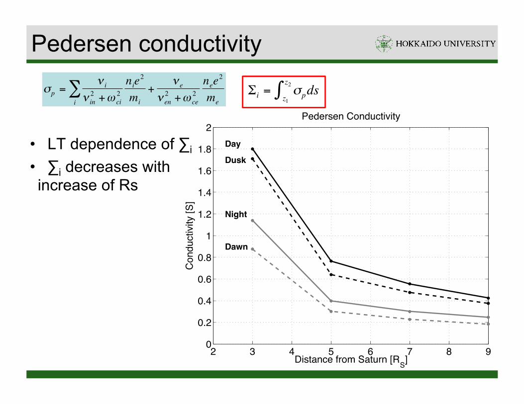
•  LT dependence of ∑i

•  ∑i decreases with increase of Rs


€

σp =ν i

ν in2 +ω ci

2nie

2

mi

+ν e

ν en2 +ω ce

2nee

2

mei∑

€

Σi = σpdsz1

z2∫

1.  Modeling of inner magnetosphere with dust-plasma interaction

2.  Modeling of ionosphere 3.  Magnetosphere-ionosphere coupling

Magnetospheric ion velocity








•  Vi depends on LT. Large dust density, D=1 RS

€


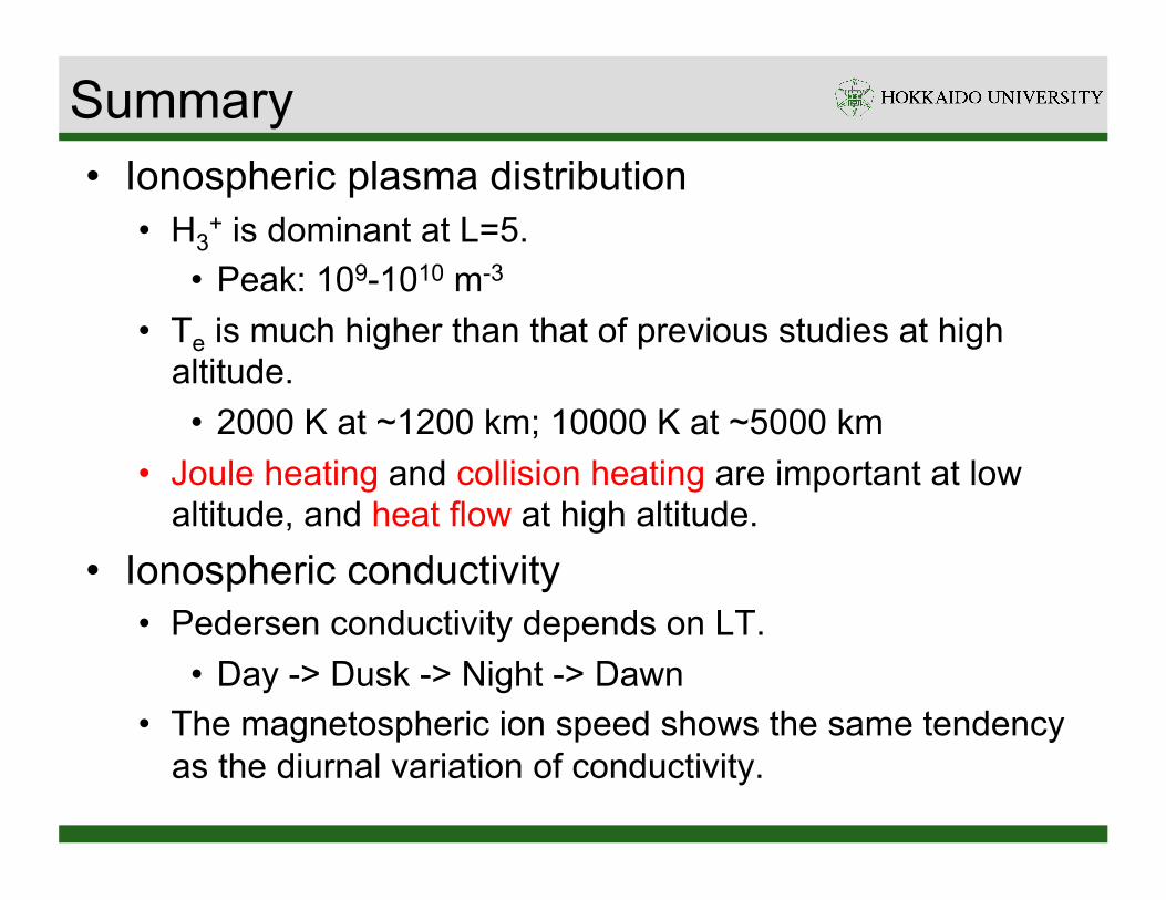
Summary •  Ionospheric plasma distribution

•  H3+ is dominant at L=5.

•  Peak: 109-1010 m-3

•  Te is much higher than that of previous studies at high altitude. •  2000 K at ~1200 km; 10000 K at ~5000 km

•  Joule heating and collision heating are important at low altitude, and heat flow at high altitude.

•  Ionospheric conductivity •  Pedersen conductivity depends on LT.

•  Day -> Dusk -> Night -> Dawn •  The magnetospheric ion speed shows the same tendency

as the diurnal variation of conductivity.

Conclusion of this thesis From Observations •  Inner magnetoshpheric ion speed is slow down from

the co-rotation speed. •  Ion speed is Keplerian in the Enceladus plume.

From Modelings •  Ion speed is slow down from the co-rotation speed due

to dust-plasma interaction and magnetosphere-ionosphere coupling.

Reference Works •  Sakai, S., S. Watanabe, M. W. Morooka, M. K. G. Holmberg, J.

–E. Wahlund, D. A. Gurnett, and W. S. Kurth (2013), Dust-plasma interaction through magnetosphere-ionosphere coupling in Saturn’s plasma disk, Planet. Space Sci., 75, 11-16, doi:10.1016/j.pss.2012.11.003.

•  Sakai, S., and S. Watanabe (2014), High-speed flow and high temperature plasma in Saturn’s mid-latitude ionosphere, in preparation.

•  Sakai, S., M. W. Morooka, J. –E Wahlund, and S. Watanabe (2014), Dusty plasma distribution of Enceladus plume observed by Cassini RPWS/LP, in preparation.

Documents

Studies on dust-plasma interaction in Saturn’s inner ...psg/doc2014/shotaro_D/sakai_D...Final examination for PhD, 4 February 2014 Studies on dust-plasma interaction in Saturn’s