Studies of Meson-Meson Interactionswithin Lattice QCDPh.D. thesisbyAttila Mih�aly

Kossuth Lajos UniversityDepartment of Theoretical PhysicsDebrecen, 1998

Contents1 Introduction 52 Lattice Quantum Chromodynamics 92.1 QCD Lagrangian . . . . . . . . . . . . . . . . . . . . . . . . . 92.2 Path Integral Approach to Quantization . . . . . . . . . . . . 102.3 Lattice Regularization . . . . . . . . . . . . . . . . . . . . . . 132.4 Fermions on the Lattice . . . . . . . . . . . . . . . . . . . . . 142.4.1 Species Doubling . . . . . . . . . . . . . . . . . . . . . 142.4.2 Wilson Fermions . . . . . . . . . . . . . . . . . . . . . 152.4.3 Kogut-Susskind Fermions . . . . . . . . . . . . . . . . 172.5 Pure and Full Lattice QCD Action . . . . . . . . . . . . . . . 192.6 Continuum Limit . . . . . . . . . . . . . . . . . . . . . . . . . 223 Meson-Meson Interactions on the Lattice 253.1 Quark Propagators . . . . . . . . . . . . . . . . . . . . . . . . 263.1.1 Random Source Technique . . . . . . . . . . . . . . . . 273.1.2 Hopping Parameter Expansion . . . . . . . . . . . . . 283.2 Field Operators and Correlation Functions . . . . . . . . . . . 303.3 Heavy-Light Meson-Meson System (MM) . . . . . . . . . . . 323.3.1 Correlation Functions . . . . . . . . . . . . . . . . . . 333.3.2 Autocorrelation of the Two-Point Function . . . . . . 353.3.3 Number of Random Sources . . . . . . . . . . . . . . . 363.3.4 MM-Potentials . . . . . . . . . . . . . . . . . . . . . . 363.3.5 Exotic Mesons as Two-Meson \Molecules" . . . . . . . 473.4 Heavy-Light Meson-Antimeson System (M �M) . . . . . . . . . 513.4.1 Correlation Functions . . . . . . . . . . . . . . . . . . 523.4.2 M �M Gluon-Exchange Potentials . . . . . . . . . . . . 533.4.3 I = 0M �M-Potentials from Lattice and Inverse Scattering 563

4 Contents3.4.4 I = 1 M �M-Potentials . . . . . . . . . . . . . . . . . . . 603.5 Simulations with an Improved Action . . . . . . . . . . . . . 633.5.1 Improved Actions and Operators . . . . . . . . . . . . 653.5.2 Numerical Results for the MM and M �M Systems . . . 674 Summary and Conclusion 75�Osszefoglal�as 79Acknowledgments 83Bibliography 85Documentation of Publications 91

Chapter 1IntroductionHadron-hadron interactions, in particular nucleon-nucleon interactions areof central importance in nuclear physics. The study of nuclei is a many-body problem which necessitates the solution of the Schr�odinger equationwith a given interaction potential. Therefore one of the most importanttasks of theoretical nuclear physics is to �nd such a potential, from whichthe deuteron properties, the nucleon-nucleon scattering phase shifts, theproperties of nuclear matter etc. | can be derived.Eisenbud and Wigner [1] and later also Okubo and Marshak [2] pointedout that the nucleon-nucleon potential must ful�ll general requirements fromthe fundamental conservation laws. Demanding invariance under space-timetranslations, Galilei transformations, rotations, time and space inversion,and further on an approximate charge symmetry, they set up a general non-relativistic, hermitian nucleon-nucleon potential. This potential includescentral, spin-spin, tensor, spin-orbit and quadratic spin-orbit terms. Thedetermination of the coe�cients of these terms leads to phenomenologicalpotentials, such as the Reid potential [3].A somewhat more fundamental derivation of the nucleon-nucleon poten-tial is possible within models assuming mesons and baryons as fundamentaldegrees of freedom. Here, the interactions between baryons are mediatedby exchange of mesons. For example, the Bonn potential [4{6] is obtainedfrom a �eld-theoretical Hamiltonian, containing nucleon-nucleon-meson andnucleon-�-meson interaction vertices. In the Paris model [7] nucleon-pionand pion-pion interactions are considered, but all contributions to the inter-action are directly derived from experiment and not calculated within a �eldtheory. 5

6 Chapter 1. IntroductionNowadays it is generally accepted that hadrons are composite particles.To systematize the numerous hadron states, in 1963 Gell-Mann proposedthat mesons should be thought of being composites of a quark and an anti-quark, whereas baryons should consist of three quarks. In this way all knownhadrons could be built up, and the model could also predict the existenceof a new hadron, called �, which was discovered one year later. There isalso experimental evidence for the existence of hadronic substructure. Theaverage hadron radius is of the order of 1 fm. Deep inelastic lepton-hadronscattering indicated the existence of scattering centers with an extent of lessthan 10�3 fm. From the scattering angular distribution observed in theseexperiments the spin of the constituents was determined to be 1=2�h. Theircharge turned out to be a fraction (+2/3 or {1/3) of the unit charge. Never-theless, up to now all attempts to isolate a single quark experimentally havefailed. The quarks are apparently enclosed in the hadrons. This phenomenonis called quark con�nement.The quark potential models of hadron-hadron interactions take the com-positeness of hadrons into account. A typical example is the non-relativisticmodel of Isgur et al. [8]. Here, one tries to derive an e�ective nucleon-nucleon potential via variational calculations with a six-quark wave-functionand a Hamiltonian, in analogy with the variational techniques used for thehydrogen molecule in atomic physics. A relativistic approach to the nucleon-nucleon interaction is the bag model [9]. Examples of bag models are theMIT-bag [10], the little-bag [11] and the cloudy-bag model [12]. A com-mon feature of quark potential and bag models is that quark con�nement isimposed arti�cially on the system by an additional constraint.All afore mentioned models contain parameters to �t the results to ex-periments. They usually yield a good quantitative outcome within a certainenergy range, but from their very construction, a fundamental understandingof the nuclear interaction cannot be obtained.The correct theory to describe the interaction between quarks is believedto be Quantum Chromodynamics (QCD). In this theory the interactions be-tween quarks are the result of the exchange of vector particles called gluons.Encouraged by the great success of Quantum Electrodynamics (QED), andas an attempt for a generalized treatment of di�erent interactions, QCDwas formulated as a quantum �eld theory based on the principle of localgauge invariance. In contrast to QED, which is an Abelian theory, QCD isformulated as a non-Abelian gauge �eld theory based on the group SU(3).This choice of the gauge group was suggested by the antisymmetrizationprocedure of the three-quark system. As a consequence the �elds carry an

7additional quantum number, called color. Quark �elds transform accord-ing to the fundamental representation of SU(3). All hadrons transform ascolor singlets, and are therefore called \color neutral". Because of the non-Abelian structure the colored gluons can couple to themselves. These selfcouplings, one believes, are responsible for quark con�nement. Nevertheless,the connection between con�nement and non-Abelian �elds is not yet totallyunderstood.QCD is an asymptotically free theory, i.e. the coupling constant is smallfor large four-momentum transfer [13, 14]. At low energies, however, thecoupling constant becomes large. Consequently, perturbation theory doesnot work in the low energy regime. Therefore the calculation of phenom-ena at nucleonic distances requires non-perturbative tools. The interest innon-perturbative methods for a fundamental treatment of QCD low energyphenomena led to the formulation of QCD on the lattice [15]. Here, quarksare de�ned on the sites of a �ctitious four-dimensional space-time lattice,whereas gauge �elds are placed on the links between the sites. The formu-lation of the theory as a path integral in euclidean space-time leads to ananalogy between the �eld theoretical vacuum expectation value and the par-tition function in statistical mechanics. In this way, within �eld theories onecan apply the well-known tools of statistical mechanics, such as analyticalseries expansions or numerical Monte Carlo simulations. Furthermore, theuse of a lattice represents the introduction of a regularization scheme for thequantum �eld theory. The momenta are restricted to the �rst Brillouin zone,therefore high momenta are cut o� and consequently ultraviolet divergencesare removed. To obtain physically relevant results from a lattice calculationone has to perform the continuum limit, that is the limit of in�nitesimallysmall lattice constants. The practical approach of the continuum limit stillposes a di�cult problem. A short overview about the basics of lattice QCDis given in Chapter 2. More detailed descriptions can be found in the stan-dard textbooks of M. Creutz [16], H.J. Rothe [17] and I. Montvay and G.M�unster [18].Within the framework of QCD, the hadron-hadron interactions are resid-ual forces between two quark clusters, each consisting of two or three quarks(mesons and baryons, respectively). The hadron-hadron forces are medi-ated for short distances by gluon exchange between the constituent quarkswhereas for longer distances the production of quark-antiquark pairs is ex-pected to be the dominating mechanism, which can be interpreted as ane�ective meson exchange. This explains why the meson exchange poten-tials give a satisfactory description of nucleon-nucleon scattering for long

8 Chapter 1. Introductiondistances, whereas quark potential and bag models are mainly successful forshort distances. Remarkably, only few attempts have been made to extracte�ective interactions, or potentials, between two composite hadrons in theframework of a lattice discretized theory [19{22]. This task is very challeng-ing since the residual interaction between two color singlets is about 10�2 to10�3 times smaller than a typical hadron mass.This work is an attempt to obtain hadron-hadron potentials in the frame-work of lattice QCD. As a simpli�cation, the interaction between two hadronsconsisting of a heavy and a light quark degree of freedom (K, B, D mesons)is investigated. Di�erent aspects of this problem are presented in Chapter3. Section 3.1 is devoted to the de�nition and simulation of quark prop-agators on the lattice, being the key quantities of our investigation. TheGreen functions describing the dynamics of the one-meson and two-mesonsystems are constructed in Section 3.2. The heavy-light approximation andthe interaction potentials between two heavy-light color singlets for variouslight-quark mass parameter are presented in Section 3.3. In Section 3.4, po-tentials between a heavy-light meson and the corresponding antiparticle arecomputed. A lattice improvement technique allowing for a re�ned analysisas well as the simulation results obtained by this technique are presented inSection 3.5. Finally, Chapter 4 is for the summary and outlook.

Chapter 2Lattice QuantumChromodynamics2.1 QCD LagrangianNowadays it is generally accepted that the theory for strong interactionsshould be Quantum Chromodynamics, since in the domain of high energyscattering QCD is highly successful. QCD was constructed along the linesof the very successful Quantum Electrodynamics (QED) as a quantizedgauge �eld theory with a local gauge symmetry. In contrast to the AbelianU(1) gauge symmetry of QED, the QCD Lagrangian is invariant under non-Abelian SU(3) gauge transformations. Whereas in QED electrons and pho-tons are the fundamental particles, in QCD quarks and gluons are the basicdegrees of freedom. Quarks are fermionic matter �elds. They transformaccording to the fundamental triplet representations of SU(3)color. Gluonsare bosonic gauge �elds and transform according to the octet representation.The QCD Lagrangian consists of a gluonic and a fermionic part,LQCD = LQCDG + LQCDF= �14F a��(x)F ��a (x) + nfXf=1 � f (x)(iD/�mf ) f (x) ; (2.1)where f is the Dirac spinor, mf the quark mass and nf the number of avors. The generalized �eld strength tensor F ��a (x) isF ��a (x) = @�A�a(x)� @�A�a(x)� gfabcA�b (x)A�c (x) ; (2.2)9

10 Chapter 2. Lattice Quantum Chromodynamicswhere a; b; c = 1; : : : ; 8 are SU(3) indices. A�a is the gauge �eld, g is thecoupling constant, and fabc are the structure constants of SU(3). D/ is anabbreviation for �D�(x), whereD�(x) = @� + igA�a (x)�a2 (2.3)is the gauge covariant derivative with the generators �a of SU(3) (Gell-Mannmatrices).The Lagrangian (2.1) allows for the formulation of QCD as a quantum�eld theory. One possible quantization is the path integral formulation ofQCD.2.2 Path Integral Approach to QuantizationSince its introduction by Feynman [23] the path integral method has becomea very important tool for elementary particle physicists. Many of the moderndevelopments in theoretical particle physics are based on this method. One ofthese developments is the lattice formulation of �eld theories. In contrast toclassical mechanics, in quantum mechanics the exact trajectory of a particlein con�guration space is not known; instead, one has to calculate transitionamplitudes like h q0t j qt0 i ; (2.4)where j qt0 i and j q0t i are eigenstates of the space coordinate operator Q(t)in the Heisenberg picture. The absolute square of the transition amplitude(2.4) is proportional to the probability that a particle which at the time t0was located at q, at the time t will be found at q0.There exist in�nitely many paths connecting the initial point with the�nal one. Feynman showed [24] that the transition amplitude (2.4) can befound by integrating over all possible paths, weighted with the phase factorexp(iS[q]), where S[q] = Z tt0dt0 L(q(t0); _q(t0)) (2.5)is the classical action. This prescription can be symbolically written in termsof a functional or path integral:h q0t j qt0 i = Z q0q D[q]eiS[q] : (2.6)

2.2. Path Integral Approach to Quantization 11Notice that while the canonical quantization goes far away from theoriginal formulation of classical mechanics, the path integral representationof Feynman reestablishes the connection with the classical action principle.The function weighting the paths is actually exp(iS[q]=�h). In the limit �h! 0this is a rapidly oscillating function. As a consequence, the contribution ofall paths to the transition amplitude (2.4) vanishes, except that of the pathfor which �S[q] = 0. This is the principle of least action which leads to theclassical equations of motion. Thus, within the path integral framework thequantization of a classical system amounts to taking into account uctuationsaround the classical path.As a possible way of quantization, the path integral formalism can be alsointroduced in �eld theories. Within QCD the vacuum expectation value ofan operator is calculated according tohO i = h 0 jO j 0 i = 1Z Z D[A] D[ ] D[ � ] eiS[A; ; � ] O(A; ; � ) ; (2.7)with the vacuum-to-vacuum transition amplitudeh 0 j 0 i � Z = Z D[A] D[ ] D[ � ] eiS[A; ; � ] : (2.8)Here the functional integration extends over all gauge �eld con�gurationsA�a(x) (Lorentz index � = 0; : : : ; 3, group index a = 1; : : : ; 8) and over allcon�gurations of the fermionic �elds �c (x) and � �c (x) (spinor index � =1; : : : ; 4, color index c = 1; 2; 3). Because of the anti-commutation relationsof the fermionic �elds these are represented by Grassmann variables.Since the weights in (2.7) and (2.8) are oscillating functions, this pathintegral representation is not suited for numerical calculations. The problemcan be overcome by formulating QCD on a four-dimensional euclidean space.This is achieved by an analytical continuation to imaginary timet = x0 ! �ix4 with real x4 : (2.9)The transition to the euclidean space from the Minkowski space can be doneby using in the formulae the replacement (2.9) whenever t appears explicitly,together with the proper replacement of the four-component quantities withthose valid in the euclidean space. In QCD, three such replacements shouldbe performed: @0 ! i@4, p0 ! ip4, and A0 ! iA4. Thus, for the euclideangluonic Lagrangian LEG one obtains:LMG = �14F a��(x)F��a (x)

12 Chapter 2. Lattice Quantum Chromodynamics= �14�F aij(x)F aij(x)� 2F a0j(x)F a0j(x) + F a00(x)F a00(x)�! �14�F aij(x)F aij(x) + 2F a4j(x)F a4j(x) + F a44(x)F a44(x)�= �14F a��(x)F a��(x) � �LEG : (2.10)Here, �; � = 0; : : : ; 3 are four indices in Minkowski space, and �; � = 1; : : : ; 4are those in Euclidean space. For the fermionic Lagrangian one obtainsLMF = � (x)(iD/�m) (x)! � � (x)(D� � +m) (x) � �LEF : (2.11)The euclidean matrices ful�l the anti-commutation relationsf �; �g = 2��� : (2.12)A possible choice for the matrices is 4 = 1 00 �1 ! ; i = 0 �i�i 0 ! ; (2.13)with the Pauli matrices �i. They are hermitian, i.e. � = y� : (2.14)With i R dx0 = R dx4 one obtains the complete euclidean actioniSM = i Z d4x (LMG + LMF ) = i Z dx0 d3x (LMG + LMF )! Z dx4 d3x (�LEG �LEF) � �SE : (2.15)The vacuum expectation value of an observable in the euclidean path integralformulation is thereforehO i = 1Z Z D[A] D[ ] D[ � ] e�SE[A; ; � ] O(A; ; � ) ; (2.16)with Z = Z D[A] D[ ] D[ � ] e�SE[A; ; � ] : (2.17)If the system is periodic in euclidean time, then Z can be viewed as a par-tition function and (2.16) has the form of a statistical ensemble averagewith a Boltzmann distribution given by exp(�SE[A; ; � ]). This allows us

2.3. Lattice Regularization 13to use well-known statistical methods to calculate expectation values. Thenon-perturbative studies of QCD are based on this simple observation.Results from the euclidean space should in principle be analytically con-tinued back to Minkowski space. For many physical problems, however, likethe calculation of the mass of a particle from the asymptotic behavior of itspropagator one can obtain results directly from the euclidean formulation.2.3 Lattice RegularizationAs we have seen in the previous section, formulating QCD in the euclideanspace-time opens up the possibility for numerical calculations. But since the�elds A, and � have in�nite degrees of freedom, at each coordinate x =(x1; x2; x3; x4), the integration measure D[A; ; � ] is still mathematically notwell de�ned. To give the path integrals a precise meaning, one discretizesboth time and space, i.e. introduces a space-time lattice, and restricts x toa multiple of a \lattice spacing" a, i.e. x = na, with n an integer. De�ningthe �elds on this euclidean space-time lattice one obtains a discrete set ofvariables. The functional integration over all �eld con�gurations simpli�esto an integration over these variables.The Fourier transform of a function f(x) de�ned on the periodic lattice~f(p) = a4Xx eipxf(x) (2.18)is periodic in p with the period p� = 2�=a. Therefore momentum is restrictedto the �rst Brillouin zone ��=a < p� � �=a. This removes ultravioletdivergences. So the introduction of a lattice provides a regularization scheme.Internal symmetries survive discretization whereas spatial symmetriesare broken. This is obvious for the euclidean Poincar�e group, which containsO(4) rotations, but on the lattice only rotations by multiples of �=2 areallowed. The enormous advantage is that local gauge invariance can bepreserved. Furthermore, in the limit a! 0 one should recover the continuumtheory. However, there is no unique choice of a discrete action ful�lling thisrequirement.

14 Chapter 2. Lattice Quantum Chromodynamics2.4 Fermions on the Lattice2.4.1 Species DoublingWhile scalar and vector �elds can be simply assigned to the sites of thelattice, the gauge �elds neccessitate a careful treatment, in order to preservegauge invariance. The association of spinors to the lattice is even moredi�cult and not yet satisfactorily solved.The euclidean free fermionic continuum action isSF = Z d4x � (x)(@� � +m) (x) : (2.19)Following the naive discretization scheme we introduce a four dimensionalspace-time lattice. With each site x of the lattice we associate an inde-pendent four-component spinor variable x. To keep the action simple, wereplace the derivative by a symmetric di�erential quotient:@� x ! 12a [ x+� � x��] : (2.20)Substituting R d4x by a4Px we arrive at the following free fermionic dis-cretized action [25]:SF = a4� 12aXx;� h � x � x+� � � x+� � xi+mXx � x x� : (2.21)Contrary to expectations, the above action does not reproduce the correctcontinuum limit, because it has a new hidden degeneracy in the fermionicdegrees of freedom. To see this let us consider the propagator of a masslessfree fermion in momentum spaceG(p) = 11aP� � sin(p�a) : (2.22)Besides the physical pole at p�a = 0 there are 15 further poles in the �rstBrillouin zone atp�a = (�; 0; 0; 0) ; (0; �; 0; 0) ; : : : ; (�; �; 0; 0) ; : : : ; (�; �; �; �) : (2.23)Thus the naively discretized action describes 16 fermions and consequentlycannot reproduce the original continuum Lagrange density in the limit a!0. This proliferation of fermions is called fermion doubling.

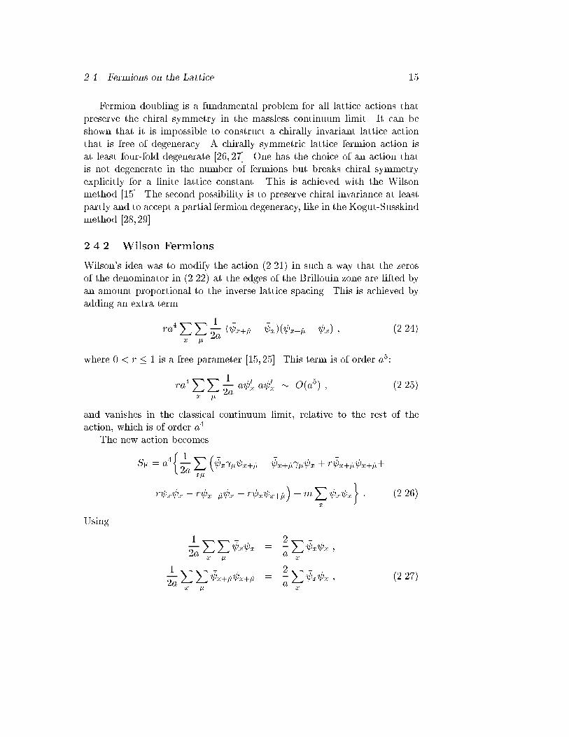
2.4. Fermions on the Lattice 15Fermion doubling is a fundamental problem for all lattice actions thatpreserve the chiral symmetry in the massless continuum limit. It can beshown that it is impossible to construct a chirally invariant lattice actionthat is free of degeneracy. A chirally symmetric lattice fermion action isat least four-fold degenerate [26, 27]. One has the choice of an action thatis not degenerate in the number of fermions but breaks chiral symmetryexplicitly for a �nite lattice constant. This is achieved with the Wilsonmethod [15]. The second possibility is to preserve chiral invariance at leastpartly and to accept a partial fermion degeneracy, like in the Kogut-Susskindmethod [28, 29].2.4.2 Wilson FermionsWilson's idea was to modify the action (2.21) in such a way that the zerosof the denominator in (2.22) at the edges of the Brillouin zone are lifted byan amount proportional to the inverse lattice spacing. This is achieved byadding an extra termra4Xx X� 12a ( � x+� � � x)( x+� � x) ; (2.24)where 0 < r � 1 is a free parameter [15, 25]. This term is of order a5:ra4Xx X� 12a a � 0x a 0x � O(a5) ; (2.25)and vanishes in the classical continuum limit, relative to the rest of theaction, which is of order a4.The new action becomesSF = a4� 12aXx� � � x � x+� � � x+� � x + r � x+� x+�+r � x x � r � x+� x � r � x x+��+mXx � x x� : (2.26)Using 12aXx X� � x x = 2aXx � x x ;12aXx X� � x+� x+� = 2aXx � x x ; (2.27)

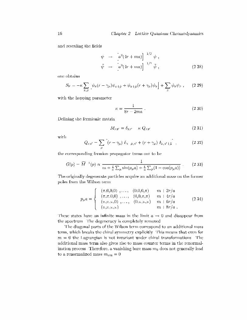
16 Chapter 2. Lattice Quantum Chromodynamicsand rescaling the �elds ! ha3(4r +ma)i�1=2 ;� ! ha3(4r +ma)i�1=2 � ; (2.28)one obtainsSF = ��Xx;� h � x(r � �) x+� + � x+�(r + �) xi+Xx � x x ; (2.29)with the hopping parameter � = 18r + 2ma : (2.30)De�ning the fermionic matrixMxx0 = �xx0 � � Qxx0 (2.31)with Qxx0 =X� h(r � �) �x+�;x0 + (r + �) �x;x0+�i ; (2.32)the corresponding fermion propagator turns out to beG(p) = fM�1(p) / 1m+ iaP� sin(p�a) + raP�(1� cos(p�a)) : (2.33)The originally degenerate particles acquire an additional mass on the formerpoles from the Wilson termp�a = 8>>><>>>: (�;0;0;0) ; : : : ; (0;0;0;�) m+ 2r=a(�;�;0;0) ; : : : ; (0;0;�;�) m+ 4r=a(�;�;�;0) ; : : : ; (0;�;�;�) m+ 6r=a(�;�;�;�) m+ 8r=a : (2.34)These states have an in�nite mass in the limit a ! 0 and disappear fromthe spectrum. The degeneracy is completely removed.The diagonal parts of the Wilson term correspond to an additional massterm, which breaks the chiral symmetry explicitly. This means that even form = 0 the Lagrangian is not invariant under chiral transformations. Theadditional mass term also gives rise to mass counter terms in the renormal-ization process. Therefore, a vanishing bare mass m0 does not generally leadto a renormalized mass mren = 0.

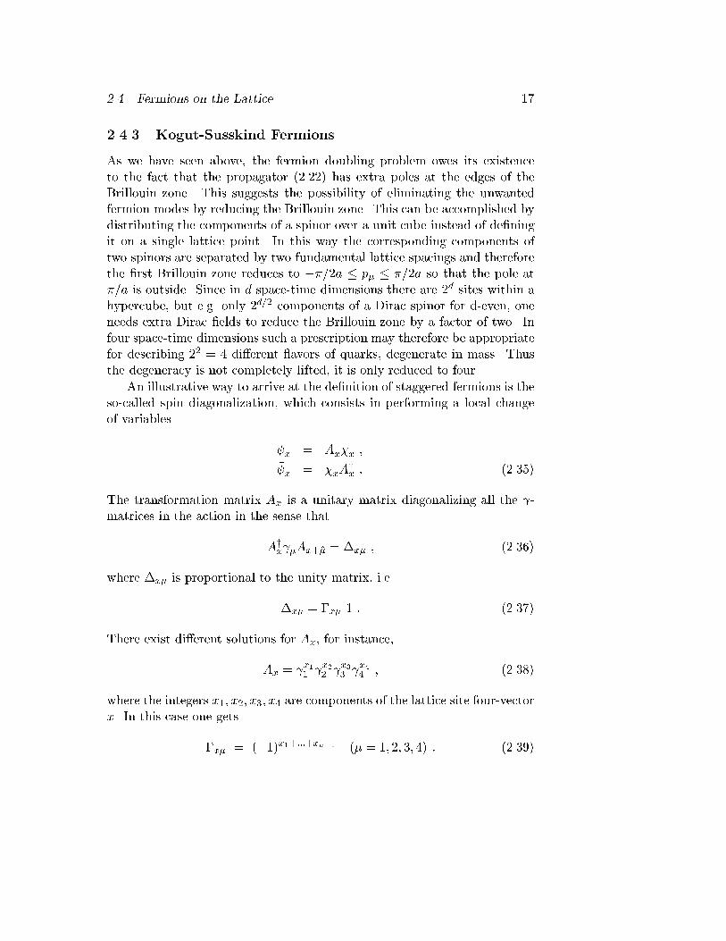
2.4. Fermions on the Lattice 172.4.3 Kogut-Susskind FermionsAs we have seen above, the fermion doubling problem owes its existenceto the fact that the propagator (2.22) has extra poles at the edges of theBrillouin zone. This suggests the possibility of eliminating the unwantedfermion modes by reducing the Brillouin zone. This can be accomplished bydistributing the components of a spinor over a unit cube instead of de�ningit on a single lattice point. In this way the corresponding components oftwo spinors are separated by two fundamental lattice spacings and thereforethe �rst Brillouin zone reduces to ��=2a � p� � �=2a so that the pole at�=a is outside. Since in d space-time dimensions there are 2d sites within ahypercube, but e.g. only 2d=2 components of a Dirac spinor for d-even, oneneeds extra Dirac �elds to reduce the Brillouin zone by a factor of two. Infour space-time dimensions such a prescription may therefore be appropriatefor describing 22 = 4 di�erent avors of quarks, degenerate in mass. Thusthe degeneracy is not completely lifted, it is only reduced to four.An illustrative way to arrive at the de�nition of staggered fermions is theso-called spin diagonalization, which consists in performing a local changeof variables x = Ax�x ;� x = ��xAyx : (2.35)The transformation matrix Ax is a unitary matrix diagonalizing all the -matrices in the action in the sense thatAyx �Ax+� = �x� ; (2.36)where �x� is proportional to the unity matrix, i.e.�x� = �x� 1 : (2.37)There exist di�erent solutions for Ax, for instance,Ax = x11 x22 x33 x44 ; (2.38)where the integers x1; x2; x3; x4 are components of the lattice site four-vectorx. In this case one gets�x� = (�1)x1+:::+x��1 (� = 1; 2; 3; 4) : (2.39)

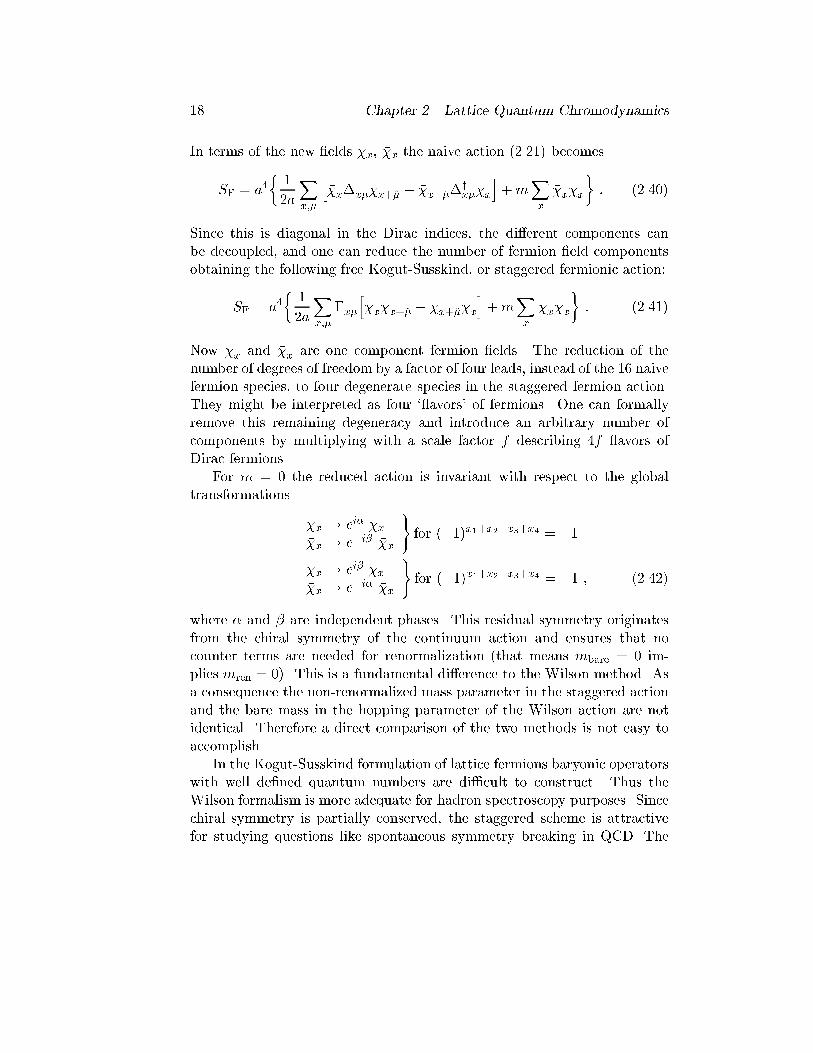
18 Chapter 2. Lattice Quantum ChromodynamicsIn terms of the new �elds �x, ��x the naive action (2.21) becomesSF = a4� 12aXx;� h��x�x��x+� � ��x+��yx��xi+mXx ��x�x� : (2.40)Since this is diagonal in the Dirac indices, the di�erent components canbe decoupled, and one can reduce the number of fermion �eld componentsobtaining the following free Kogut-Susskind, or staggered fermionic action:SF = a4� 12aXx;� �x�h��x�x+� � ��x+��xi+mXx ��x�x� : (2.41)Now �x and ��x are one component fermion �elds. The reduction of thenumber of degrees of freedom by a factor of four leads, instead of the 16 naivefermion species, to four degenerate species in the staggered fermion action.They might be interpreted as four ` avors' of fermions. One can formallyremove this remaining degeneracy and introduce an arbitrary number ofcomponents by multiplying with a scale factor f describing 4f avors ofDirac fermions.For m = 0 the reduced action is invariant with respect to the globaltransformations �x ! ei� �x��x ! e�i� ��x ) for (�1)x1+x2+x3+x4 = 1�x ! ei� �x��x ! e�i� ��x ) for (�1)x1+x2+x3+x4 = �1 ; (2.42)where � and � are independent phases. This residual symmetry originatesfrom the chiral symmetry of the continuum action and ensures that nocounter terms are needed for renormalization (that means mbare = 0 im-plies mren = 0). This is a fundamental di�erence to the Wilson method. Asa consequence the non-renormalized mass parameter in the staggered actionand the bare mass in the hopping parameter of the Wilson action are notidentical. Therefore a direct comparison of the two methods is not easy toaccomplish.In the Kogut-Susskind formulation of lattice fermions baryonic operatorswith well de�ned quantum numbers are di�cult to construct. Thus theWilson formalism is more adequate for hadron spectroscopy purposes. Sincechiral symmetry is partially conserved, the staggered scheme is attractivefor studying questions like spontaneous symmetry breaking in QCD. The

2.5. Pure and Full Lattice QCD Action 19price one has to pay is that the degeneracy cannot be completely avoided,for reasons mentioned in Section 2.4.1. In practice one introduces a factorf = 1=4 in the action to account for the remaining degeneracy. Whetherthis concept gives the correct continuum limit is an unsolved problem.2.5 Pure and Full Lattice QCD ActionThe lattice regularization of gauge �elds should be performed by preservinggauge invariance. One can easily verify that a naive discretization by simplyassigning the vector potentials to the sites and substituting all derivativeswith �nite di�erential quotients would violate local gauge invariance for �nitelattice spacing a.The gluonic �elds were introduced in the Dirac part of the continuumQCD Lagrangian (2.1) by demanding invariance of the fermionic action withrespect to the SU(3) gauge transformations, and adding a gauge-invariantkinetic term. The de�nition of the gauge �elds on the lattice can be obtainedby following this procedure. Let us consider the free fermionic discretizedaction (2.21), where the �elds x and � x are now three-component �eldsin color space (being also four-component spinor variables) so that the La-grangian is invariant under the global transformations x ! g x� x ! � xg�1 ; (2.43)where g is an element of SU(3). The next step consists in requiring thetheory to be invariant under local SU(3) transformations, with the groupelement gx depending on the lattice site. For this, one has to make thefollowing substitutions in (2.21):� x x+� ! � xUx� x+�� x+� x ! � x+�Ux+�;�� x : (2.44)The factors Ux� and Ux+�;�� are determined by the line integral of A� alongthe link, e.g. Ux� � P exp �i Z x+a�x gA� � dy! ; (2.45)where the P-operator path-orders the A�'s along the integration path. No-tice that Ux� and Ux+�;�� are elements of the SU(3) group, transforming

20 Chapter 2. Lattice Quantum Chromodynamicsaccording to Ux� ! gxUx�g�1x+�Ux+�;�� ! gx+�Ux+�;��g�1x ; (2.46)and satisfying the relationUx+�;�� = U yx� = U�1x� : (2.47)In contrast to the matter �elds, the group elements Ux� live on the linksconnecting two neighboring lattice sites; hence, they are referred to as \linkvariables".Making the substitutions (2.44) in eq. (2.21), we obtain the followinggauge-invariant lattice fermionic action:SF = a4� 12aXx;� h � x �Ux� x+� � � x+� �U yx� xi+mXx � x x� : (2.48)In this formula the color, Dirac and avor indices are omitted. Using (2.45),SF yields formally the correct continuum limit:SF a!0�! Z d4x � (x)(D� � +m) (x) : (2.49)The change of (2.48) to the Wilson and staggered fermionic actions (2.29)and (2.41) is obvious. In the staggered scheme the �elds become three-component vectors � in color space and should be coupled to the matrix-valued link variables in the same gauge-invariant way. The gauge-invariantstaggered fermionic action reads:SF = a4� 12aXx;� �x�h��xUx��x+� � ��x+�U yx��xi+mXx ��x�x� : (2.50)It can be rewritten in terms of dimensionless lattice variables, by makingthe replacements m ! 1a m ;��x ! 1a3=2 ��x ; (2.51)�x ! 1a3=2 �x :

2.5. Pure and Full Lattice QCD Action 21Then the lattice version of (2.50) applicable in computer codes isSF =Xx;� 12�x�h��xUx��x+� � ��x+�U yx��xi+mXx ��x�x : (2.52)The lattice form of the gluonic Lagrange density should also be gaugeinvariant. There is no unique way of constructing the lattice Lagrangianbut it has to converge to the continuum Lagrangian for a ! 0. Since Ux�transforms according to (2.46), the simplest gauge-invariant quantity onecan build from the group elements Ux�, is the trace of the path orderedproduct of link variables along the boundary of an elementary plaquette:Upl;��(x) = Ux�Ux+�;�U yx+�;�U yx� : (2.53)The gauge invariant expression [15]SG = � Xpl �1� 13 ReTrUpl� ; (2.54)with the inverse coupling constant � = 6=g2, and the sum extending overall distinct plaquettes on the lattice, converges to the continuum action fora! 0 SG a!0�! Z d4x 14F��(x)F��(x) : (2.55)Thus the action (2.54) | referred to as the Wilson plaquette action | isone possible choice of the gluonic action on the lattice. Together with theaction (2.50) we now have a gauge-invariant lattice regularized version ofQCD.The persistence of the exact gauge invariance has several practical advan-tages. With gauge invariance, the quark-gluon, three-gluon, and four-gluoncoupling constants in QCD are all equal, and the bare gluon mass is zero.Without gauge invariance, each of these couplings must be tuned indepen-dently and a gluon mass introduced to recover QCD. Tuning many param-eters in a numerical simulation is very expensive. Continuous symmetrieslike Lorentz invariance can be given up with less cost because the remainingdiscrete symmetries of the lattice, though far less restrictive, are still su�-cient to prevent the introduction of new interactions with new couplings (atleast to lowest order in a).In contrast to QED, the pure gauge sector of QCD describes a highlynon-trivial interacting theory. The self couplings of the gauge potentials are

22 Chapter 2. Lattice Quantum Chromodynamicsbelieved to be responsible for quark con�nement. This is the reason why thestudies of the pure gauge sector of QCD are of great interest. Furthermore,path integrals involving Grassmann variables are di�cult to handle. Thereare some phenomenological facts in low energy hadron physics like the OZIrule [30] or the approximate linearity of Regge trajectories [31] which suggestthat closed quark loops have only a small e�ect. Most of the numerical QCDcalculations have been performed in the pure gauge sector or in the so-called quenched approximation [32, 33] where the e�ects of pair productionprocesses are neglected. The pure gluonic expectation value of an observableis hO i = 1Z Ylinks Z dUx� O(U) e�SG ; (2.56)with the partition functionZ = Ylinks Z dUx� e�SG : (2.57)The integration measure with the following featuresZ dU = 1Z dU f(U) = Z dU f(V U) = Z dU f(UV ) ; V 2 SU(3) (2.58)is called Haar's measure. In contrast to a path integral in the continuum,(2.56) and (2.57) comprise only a �nite number of integrals over the gaugegroup. No gauge �xing is needed for gauge invariant observables. A four-dimensional hyper-cubic lattice with linear dimension N has 4N4 links. Anintegration over the full gauge group SU(3), for example over the eight Eulerangles, has to be performed on each link, resulting in 32N4 integrals over acompact interval.2.6 Continuum LimitRegularization is a mathematical tool to make calculations possible. Ina renormalizable theory, the results are independent of the regularizationscheme. Thus the dependence of observables on the lattice regularizationwith the lattice spacing a as a cuto� parameter has to vanish in the contin-uum limit, and all symmetries like for example euclidean rotational invari-ance have to be restored. However, this limit is di�cult to achieve.

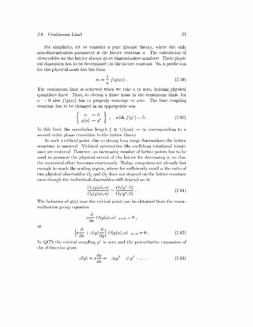
2.6. Continuum Limit 23For simplicity, let us consider a pure gluonic theory, where the onlynon-dimensionless parameter is the lattice constant a. The calculation ofobservables on the lattice always gives dimensionless numbers. Their physi-cal dimension has to be determined via the lattice constant. So, a predictionfor the physical mass has the formm = 1a f(g(a)) : (2.59)The continuum limit is achieved when we take a to zero, holding physicalquantities �xed. Thus, to obtain a �nite mass in the continuum limit, fora ! 0 also f(g(a)) has to properly converge to zero. The bare couplingconstant has to be changed in an appropriate way( a ! 0g(a) ! g� ) ; with f(g�) = 0 : (2.60)In this limit the correlation length � � 1=(ma) ! 1 corresponding to asecond order phase transition in the lattice theory.At such a critical point, due to strong long range uctuations the latticestructure is smeared. Violated symmetries like euclidean rotational invari-ance are restored. However, an increasing number of lattice points has to beused to preserve the physical extent of the lattice for decreasing a, so thatthe numerical e�ort increases enormously. Today, computers are already fastenough to reach the scaling region, where for su�ciently small a the ratio oftwo physical observables O1 and O2 does not depend on the lattice constanteven though the individual observables still depend on it:O1(g(a); a)O2(g(a); a) ' O1(g�; 0)O2(g�; 0) : (2.61)The behavior of g(a) near the critical point can be obtained from the renor-malization group equationa dda O(g(a); a) ja!0 = 0 ;or ha @@a + �(g) @@g i O(g(a); a) ja!0 = 0 : (2.62)In QCD the critical coupling g� is zero and the perturbative expansion ofthe �-function gives �(g) = adgda = ��0g3 � �1g5 + : : : : (2.63)

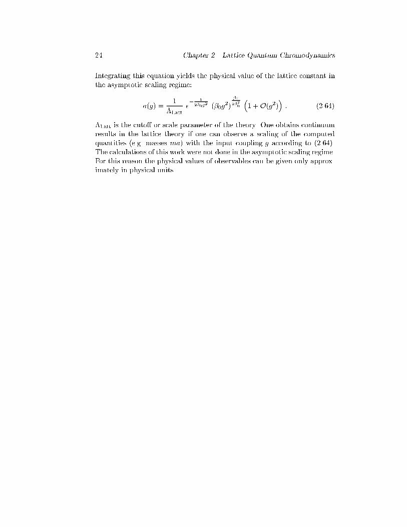
24 Chapter 2. Lattice Quantum ChromodynamicsIntegrating this equation yields the physical value of the lattice constant inthe asymptotic scaling regime:a(g) = 1�Latt e� 12�0g2 (�0g2) �12�20 �1 +O(g2)� : (2.64)�Latt is the cuto� or scale parameter of the theory. One obtains continuumresults in the lattice theory if one can observe a scaling of the computedquantities (e.g. masses ma) with the input coupling g according to (2.64).The calculations of this work were not done in the asymptotic scaling regime.For this reason the physical values of observables can be given only approx-imately in physical units.

Chapter 3Meson-Meson Interactionson the LatticeThe various models for the nucleon-nucleon interaction { as outlined in theIntroduction { often render a decent description of the experimental data andto some extent give interesting ideas for the underlying interaction mecha-nism. Nevertheless, their theoretical foundations are inadequate for a fun-damental understanding of hadron dynamics. Within the meson exchangemodels, like Bonn and Paris potentials, the basic QCD degrees of freedom,quarks and gluons, are not taken into account. On the other hand, the bagand quark potential models use arti�cially introduced boundary conditionsor con�nement potentials to ensure quark con�nement. All these modelshave various parameters and are ultimately based on phenomenology. Forthe case of meson-meson interactions the situation is worse. The relatedexperimental information is very poor and therefore less phenomenologicalmodels have been developed. One of the aims of modern theoretical nuclearand elementary particle physics is to describe hadron-hadron interactionsfrom �rst principles. The most promising framework for such investigationsis lattice QCD, not least because of the steadily increasing computer power.Remarkably, only few attempts have been made to extract potentials be-tween two composite hadrons from the lattice [19{22]. Earlier calculationsof nucleon-nucleon forces with static quarks have demonstrated that the po-tential between two three-quark clusters is attractive [21]. A hard repulsivecore of the potential, as suggested by experiments and their interpretation,could not be observed in the region where the two nucleons have relativedistance close to zero. 25

26 Chapter 3. Meson-Meson Interactions on the LatticeIn the following a method to obtain interaction potentials in QCD isdeveloped. In particular, the interaction between two heavy-light mesonsis investigated. The role of the heavy quarks is to localize the mesons sothat their relative distance ~r becomes well de�ned. The computation ofthe potential is then based on two-meson time-correlation matrices. Sincethis method employs dynamics, using quark propagators, in addition to thestatic heavy-quark gluon-exchange interaction, the calculation will includethe e�ects of interactions between gluons and light quarks, as well as light-quark exchange. Some simulations will also include the e�ects of sea quarks.3.1 Quark PropagatorsThe expectation value of products of quark �elds can be expressed in termsof two-point correlation functions of the typeh a�(x) � b�(x0)iF = R D[ ] D[ � ] a�(x) � b�(x0) e� � M R D[ � ] D[ ] e� � M = (M�1(U))ab��(x; x0) = Gab��(x; x0) : (3.1)The quark propagators G represent the basic quantities not only in hadronspectroscopy, but also many investigations involving hadron systems.Most of the computational e�ort of a calculation involving fermions goesinto constructing fermion propagators. That is, one wants to solveM(x; y)G(y; z) = �(x� z) ; (3.2)whereM(x; y) is the discretized fermion matrix. SinceM non-zero elementsin the order of the volume square, this is a problem of sparse matrix inversion.It is usually not possible to construct or store G(x; y) for all x and y since thisinvolves �nding on the order of (volume)2 numbers. Instead, one typicallyconstructs G(x; y) for all x and some selected points y by solvingM(x; y) ~G(y; z) = Y (z) ; (3.3)that is, ~G(y; z) is the vector M�1Y .In the following we employ the Kogut-Susskind formalism. The fermionmatrix of the Kogut-Susskind Lagrangian is(MKS)xx0 = 12a X� �x�[�x+�;x0 Ux� � �x;x0+� U yx0�] +m �xx0 : (3.4)

3.1. Quark Propagators 27The �x� are phases playing the role of the Dirac matrices in the Kogut-Susskind discretization (see Section 2.4.3). The size of this matrix is (3 �N3s �Nt)2, where Ns and Nt are the numbers of lattice points in space andin time direction, and the factor 3 are the color degrees of freedom. Evenfor a very small lattice like N3s � Nt = 43 � 8 MKS becomes a rather bigmatrix of dimension (1536�1536). Due to the large memory and CPU timerequirements instead of a direct numerical inversion of MKS one relies onstochastic methods.3.1.1 Random Source TechniqueThis method for inversion of large matrices employs complex vectors withrandom number components. Usually in studies of time evolution of quarksystems we need quark propagators of the type G(t; t0). They can be ob-tained by using in (3.3) sources which are non-zero only on one time slicet0 Yi;a(~x; x4) = R(t0)i;a (~x )�x4;t0 ; (3.5)where R is a complex random vector de�ned in color and coordinate spacewith 3L3 random number components (random sources) [34, 35]. For anaverage over NR random sources one has within statistical errors1NR NRXi=1R�i;a(~x )Ri;b(~y ) = �~x;~y �a;b : (3.6)Solving X~yy4 Xb (G�1)ab(~x; x4; ~y; y4)I(t0)i;b (~y; y4) = R(t0)i;a (~x ) �x4;t0 (3.7)for all vectors Ri of the ensemble (i = 1; : : : ; NR) gives a solution vector Iifor each source RiI(t0)i;a (~x; x4) =X~yb Gab(~x; x4; ~y; t0)R(t0)i;b (~y ) : (3.8)With equation (3.6) single matrix elements of the propagator can be esti-matedGab(~y; t; ~x; t0) = (M�1)ab(~y; t; ~x; t0) = 1NR NRXi=1 I(t0)i;a (~y; t)R�(t0)i;b (~x ) : (3.9)

28 Chapter 3. Meson-Meson Interactions on the LatticeEquation (3.7) must be solved for each gauge �eld con�guration and foreach vector R. To keep the CPU times for the calculation of the quark prop-agator reasonably small, one has to use an e�ective algorithm for its solution.Since the matrix M = G�1 is very large and sparse an iterative method to�nd a solution is a good choice. When choosing such a method, a matrixinversion problem has to be taken into account. The largest eigenvalue ison the order of m. For small m this means that M is ill conditioned: theratio of its largest to smallest eigenvalue diverges as m! 0. In practice, themore ill-conditioned the matrix, the harder it is to invert. This is why onegenerally does not work at the physical value of the quark mass. Instead,one is restricted to unphysically heavy values of the quark mass.There have been a number of diagnostic studies of matrix inversion al-gorithms [36]. At present it seems that the most robust algorithm, with thebest behavior for small quark mass, is the conjugate gradient algorithm [37].3.1.2 Hopping Parameter ExpansionThe quark propagator G can also be computed within the so-called hoppingparameter expansion. Let us write the fermionic action (2.52) in the formSF = mXx;y ��xKxy[U ]�y ; (3.10)where Kxy[U ] are matrices in color space:Kxy[U ] = �xy1� 12mMxy : (3.11)The only non-vanishing matrices Mxy are those connecting neighboring lat-tice sites: Mxx+� = ��x�Ux�Mxx�� = �x�U yx��;� : (3.12)The inverse of K is the fermion propagator for a given link-variable con�g-uration. For large bare quark mass m we can expand K�1 in powers of thehopping parameter 1=2m in a Neumann series:K�1[U ] = �1� 12mM��1 = 1Xl=0 � 12m�`M `; (3.13)

3.1. Quark Propagators 29where M ` is a product of ` matrices Mxy connecting neighbouring latticesites, which are given in (3.12). The corresponding expression for the matrixelements of K�1 reads:K�1xa;yb[U ] = �xy�ab + 12m(Mxy)ab+ 1Xl=2 � 12m�`Xxi (Mxx1Mx1x2 � � �Mx`�1y)ab : (3.14)Using the fact that Mxy connects only nearest neighbors on the lattice, thecontributions to K�1xa;yb[U ] of order (1=2m)` can be computed according tothe following rules:i) Consider all possible paths of length ` on the lattice starting at thelattice site x and terminating at the site y.ii) Associate with each link base at x and pointing in the �� directionthe matrices (3.12).iii) For each path, take the ordered product of all these matrices followingthe arrow pointing from x to y, and take the ab-matrix element of thisexpression.iv) Sum over all possible paths leading from x to y.It is easy to see that the matrices M in (3.12) have the following sym-metry property: Myb;xa = �M�xa;yb : (3.15)We can obtain a relation between the quark propagator and the antiquarkpropagator by taking the hermitian conjugate of (3.14), and making use of(3.15): G(y; x) = (�1)P�(x�+y�)Gy(x; y) : (3.16)Here the \dagger" refers to color indices only. This symmetry is related toCPT invariance, and is the staggered analog of the relationG(y; x) = 5Gy(x; y) 5; (3.17)for the Wilson (naive) fermions. These equations are very useful since ifwe compute e.g. the propagators of the type G(t; t0) using the algorithmspresented in the previous sections, an extra evaluation of the propagators ofthe type G(t0; t) is not necessary.

30 Chapter 3. Meson-Meson Interactions on the Lattice3.2 Field Operators and Correlation FunctionsSince the nucleon-nucleon system containing six light quarks is beyond thecurrent limits of computation, in this section the correlators containing thedynamics of two mesons are derived. In principle the method can be directlyextended for the case of baryons. The propagators for the two-meson systemwere initially derived within a QED2+1 model [38{42], the investigations wereextended later to QCD3+1 [43{47].The computation of hadron propagators in Kogut-Susskind formalismbears a few technical complications related to the assignment of avor, spaceand spin indices [48{50]. In this formalism the quark operators are nonlocaloperators which live on elementary hypercubes of the lattice. Thus a mesoninterpolating �eld can be de�ned as�AB(x) = �q(x)(�A ��B)q(x) (3.18)where �A and �B are two of the 16 matrices �b = b11 : : : b44 and b labelsthe location in the hypercube (bi = 0 or 1). By convention, �A acts onspin indices and �B acts on avor indices. If �A = �B then the operator�A � �AA is local. Otherwise it involves combinations of �eld operators atdi�erent locations in the fundamental hypercube. One must either gauge �xbefore measurement or explicitly include link factors connecting the sites.If the operator is local then�A(x) =Xb �Ab ��b(x)�b(x) (3.19)and � is 1 or {1 depending on whether �B and �A commute or anticommute.In practice this means that a local channel tends to have two particles ofopposite parity. This is a characteristic of the Kogut-Susskind formalismcausing a special behavior of the correlators. There are four possibilities forlocal operators: they are (a) � = 5, �b = (�1)x (pseudoscalar) (b) � = 1and 0 5, �b = 1 (scalar and pseudoscalar) (c) � = 3 and 2 1, �b = (�1)b3(vector and tensor) (d) � = 0 3 and 5 1, �b = (�1)b1+b2 (vector and axialvector). Thus a pseudoscalar meson �eld with momentum ~p = 2�L (k1; k2; k3)has the form: �~p(t) = 1V X~x (�1)x1+x2+x3+tei~p�~x ��f (~xt)�f 0(~xt) ; (3.20)where f and f 0 are now the avors of the Grassmann �elds and V = 3 �Nx �Ny � Nz. Meson-meson �elds � with total momentum ~P = 0 and spatial

3.2. Field Operators and Correlation Functions 31separation ~r then can be de�ned as�~r(t) =X~p e�i~p�~r��~p(t)�~p(t): (3.21)Correlations of these �eld operators contain information about the dynam-ics of the two-quark and four-quark systems and, ultimately, the e�ectiveresidual meson-meson interaction.The two-point correlator, describing the propagation of one meson onthe lattice is C(2)(t; t0) = [h�y~p(t)�~p(t0)i � h�y~p(t)ih�~p(t0)i]~p=0: (3.22)The four-point time correlation matrix describes the propagation of two in-teracting mesons on the lattice:C(4)~r~s (t; t0) = h�y~r(t)�~s(t0)i � h�y~r(t)ih�~s(t0)i: (3.23)Here ~r and ~s are relative separations of the meson-meson system. The ex-pressions in (3.22) and (3.23) can be worked out in terms of contractionsbetween the Grassmann �elds: : : n�f (x) : : : n��f 0 (x0) : : : = �ff 0 nGxx0 ; (3.24)where n indicates the partners of contraction and (G) is the quark propaga-tor. We obtain:C(2)(t; t0) = 1V 2 hX~x;~y Tr(Gy~yt;~xt0G~yt;~xt0)i= 1V 2 hX~x;~y Xa;b jGab~yt;~xt0 j2i (3.25)C(4)~r~s (t; t0) = C(4A) + C(4B) � C(4C) � C(4D)= + ����TTTT � ��TT6 � ��TT? ; (3.26)where C(4A)~r~s (t; t0) = D 1V 2 X~x;~y Tr(G~x+~rt;~yt0Gy~x+~rt;~yt0)� Tr(G~xt;~y�~st0Gy~xt;~y�~st0)E (3.27)

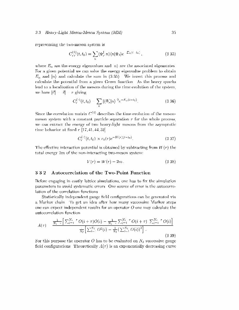
32 Chapter 3. Meson-Meson Interactions on the Latticer

H+

e-

e-

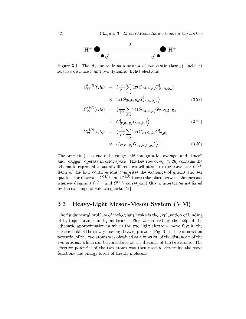
H+Figure 3.1: The H2 molecule as a system of two static (heavy) nuclei atrelative distance r and two dynamic (light) electrons.C(4B)~r~s (t; t0) = D 1V 2 X~x;~y Tr(G~x+~rt;~yt0Gy~x+~rt;~yt0)� Tr(G~xt;~y+~st0Gy~xt;~y+~st0)E (3.28)C(4C)~r~s (t; t0) = D 1V 2 X~x;~y Tr(Gy~x+~rt;~yt0G~x+~rt;~y�~st0� Gy~xt;~y�~st0G~xt;~yt0)E (3.29)C(4D)~r~s (t; t0) = D 1V 2 X~x;~y Tr(G~x+~rt;~yt0Gy~xt;~yt0� G~xt;~y�~st0Gy~x+~rt;~y�~st0)E : (3.30)The brackets h: : :i denote the gauge �eld con�guration average, and \trace"and \dagger" operate in color space. The last row of eq. (3.26) contains theschematic representations of di�erent contributions to the correlator C(4).Each of the four contributions comprises the exchange of gluons and seaquarks. For diagrams C(4A) and C(4B) those take place between the mesons,whereas diagrams C(4C) and C(4D) correspond also to interaction mediatedby the exchange of valence quarks [51].3.3 Heavy-Light Meson-Meson System (MM)The fundamental problem of molecular physics is the explanation of bindingof hydrogen atoms in H2 molecule. This was solved by the help of theadiabatic approximation in which the two light electrons move fast in theelectric �eld of the slowly moving (heavy) protons (Fig. 3.1). The interactionpotential of the two atoms was obtained as a function of the distance r of thetwo protons, which can be considered as the distance of the two atoms. Thee�ective potential of the two atoms was then used to determine the wavefunctions and energy levels of the H2 molecule.

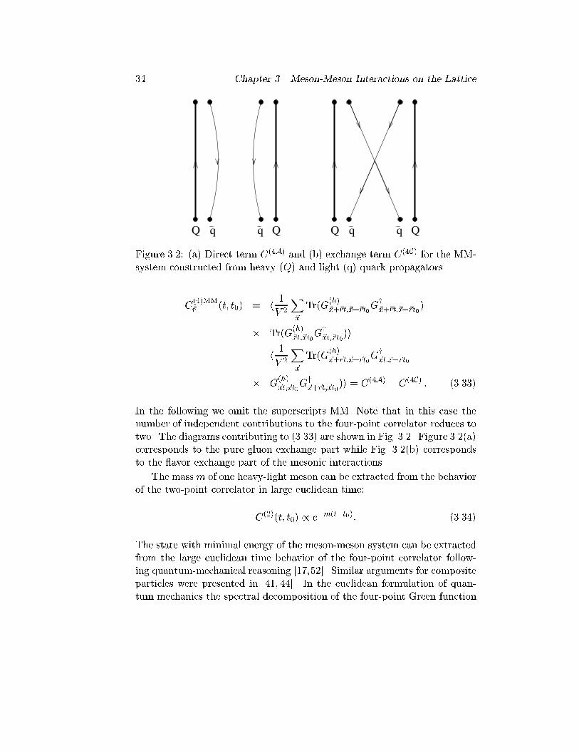
3.3. Heavy-Light Meson-Meson System (MM) 33Here an analogous problem is considered|a \hadronic molecule" con-sisting of two heavy-light mesons, in which the heavy quarks are treated asstatic colour sources, playing the role of the (slow) atomic nuclei. The gluonsand light quarks play the role of the fast degrees of freedom. In additionto the static heavy-quark gluon-exchange interaction, this calculation willinclude the e�ects of interactions between gluons and light quarks, as wellas light-quark exchange. Some simulations will also include the e�ects of seaquarks.By making one constituent quark degree of freedom of the meson veryheavy one also reduces the complexity of the formulae (3.27){(3.30) andthe heavy-light meson-meson system becomes less costly to simulate. Thissystem contains only two light valence quarks. As such, one is still quite farfrom a direct simulation of the nucleon problem. However, as all nuclei arehadronic molecules, the qualitative conclusions obtained for this case shouldbe somewhat universal. The resulting interaction potentials are of furtherinterest because they might be used for quantum-mechanical investigationsof the two-meson states in a search for exotic particles which are stableagainst strong decay.3.3.1 Correlation FunctionsThe correlators describing the resulting heavy-light mesons, as well as thesystem of two such mesons (MM) can be obtained from (3.25){(3.30) by re-placing e.g. each quark propagator with the corresponding heavy quark prop-agator, which can be taken from the hopping-parameter expansion (3.14).We only use the lowest order of the expansion so that the heavy quarksrepresent �xed color sources. Thus e.g. the heavy-antiquark propagator isgiven by G(h)~xt0;~xt = � 12mha�k [�~x4]k kYj=1Ux=(~x;ja);�=4 ; (3.31)with a similar expression for the quark propagator. The heavy quark massmh only gives rise to an irrelevant multiplicative factor in the static approx-imation and is set to mha = :5. The phase factors �~x4 = (�1)(x1+x2+x3)=ain the Kogut{Susskind formulation are remnants of the Dirac matrices andk = (t � t0)=a. Since G(h)~yt;~xt0 � 0 for ~x 6= ~y, all o�-diagonal elements of thecorrelation matrix (3.26) vanish, and we obtain:C(2)MM(t; t0) = h 1V 2 X~x Tr(Gy~xt;~xt0G(h)~xt;~xt0)i (3.32)

34 Chapter 3. Meson-Meson Interactions on the Lattice

q QqQ qQqQFigure 3.2: (a) Direct term C(4A) and (b) exchange term C(4C) for the MM-system constructed from heavy (Q) and light (q) quark propagators.C(4)MM~r (t; t0) = h 1V 2 X~x Tr(G(h)~x+~rt;~x+~rt0Gy~x+~rt;~x+~rt0)� Tr(G(h)~xt;~xt0Gy~xt;~xt0)i� h 1V 2 X~x Tr(G(h)~x+~rt;~x+~rt0Gy~xt;~x+~rt0� G(h)~xt;~xt0Gy~x+~rt;~xt0)i = C(4A) � C(4C) : (3.33)In the following we omit the superscripts MM. Note that in this case thenumber of independent contributions to the four-point correlator reduces totwo. The diagrams contributing to (3.33) are shown in Fig. 3.2. Figure 3.2(a)corresponds to the pure gluon exchange part while Fig. 3.2(b) correspondsto the avor exchange part of the mesonic interactions.The massm of one heavy-light meson can be extracted from the behaviorof the two-point correlator in large euclidean time:C(2)(t; t0) / e�m(t�t0): (3.34)The state with minimal energy of the meson-meson system can be extractedfrom the large euclidean time behavior of the four-point correlator follow-ing quantum-mechanical reasoning [17,52]. Similar arguments for compositeparticles were presented in [41, 44]. In the euclidean formulation of quan-tum mechanics the spectral decomposition of the four-point Green function

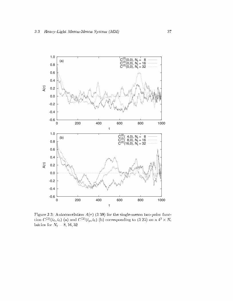
3.3. Heavy-Light Meson-Meson System (MM) 35representing the two-meson system isC(4)~r~s (t; t0) =Xn h�y~rjnihnj�~sie�En(t�t0) ; (3.35)where En are the energy eigenvalues and jni are the associated eigenstates.For a given potential we can solve the energy eigenvalue problem to obtainEn and jni and calculate the sum in (3.35). We invert this process andcalculate the potential from a given Green function. As the heavy quarkslead to a localization of the mesons during the time evolution of the system,we have j~rj = j~sj = r givingC(4)r (t; t0) =Xn jh�yrjnij2e�En(t�t0): (3.36)Since the correlation matrix C(4) describes the time evolution of the meson-meson system with a constant particle separation r for the whole process,we can extract the energy of two heavy-light mesons from the asymptotictime behavior at �xed r [17, 41, 44, 52]C(4)r (t; t0) / c4(r)e�W (r)(t�t0): (3.37)The e�ective interaction potential is obtained by subtracting from W (r) thetotal energy 2m of the non-interacting two-meson system:V (r) =W (r)� 2m: (3.38)3.3.2 Autocorrelation of the Two-Point FunctionBefore engaging in costly lattice simulations, one has to �x the simulationparameters to avoid systematic errors. One source of error is the autocorre-lation of the correlation functions.Statistically independent gauge �eld con�gurations can be generated viaa Markov chain. To get an idea after how many successive Markov stepsone can expect independent results for an operator O one may calculate theautocorrelation functionA(�) = 1NI�� hPNI��i=1 O(i+ �)O(i) � 1NI�� PNI��i=1 O(i+ �) PNI��i=1 O(i)i1NI hPNIi=1O2(i) � 1NI (PNIi=1O(i))2i : (3.39)For this purpose the operator O has to be evaluated on NI successive gauge�eld con�gurations. Theoretically A(�) is an exponentially decreasing curve

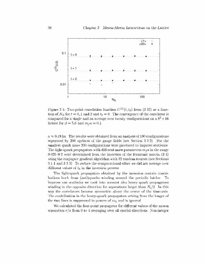
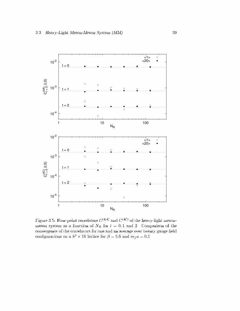
36 Chapter 3. Meson-Meson Interactions on the Latticein the limit � !1. After �0 iterations the function A is close enough to zeroto expect independent results for O when performing �0 sweeps between twomeasurements. In Figure 3.3 we plot A(�) for O = C(2)(t0; t0) (a), and forO = C(2)(tp; t0) (b) for various time extents Nt = 8; 16; 32 of a 43�Nt lattice.With our choice of the random sources we �xed t0 = 0. The minimum of thecorrelation function on a periodic lattice is at tp = Nt=2. The inverse gluoncoupling is � = 5:2. Sea quarks with mass mqa = 0:1 and nf = 3 avors areincluded in the simulation. The mass of the valence quarks is alsomfa = 0:1.From Figure 3.3 it can be seen that for � > 150 independent results for themeson two-point function can be expected.3.3.3 Number of Random SourcesIn this section we try to �nd out how many random sources have to beemployed to obtain reliable results for the correlators. For this purpose thetwo-point correlator of a heavy-light meson (3.32) is calculated in a quenchedsimulation on a 83 � 16 lattice for � = 5:6 and mfa = 0:1. In Fig. 3.4 themeson correlator is plotted against the number of random sources on a doublelogarithmic scale. The largest ensemble consisted of NmaxR = 128 randomsources. The results from a single gauge �eld con�guration are comparedwith the averages over twenty gauge �elds for t = 0; 1 and 2. In both casesthe correlator converges reasonably well above NR = 16. The behaviorof the correlator becomes worse for larger �nal times t. As expected, theconvergence of the correlator with increasing NR improves for averages overmore gauge �elds.In Fig. 3.5 we show a similar comparison for the two contributions tothe heavy-light meson-meson correlator (3.33) from a single gauge �eld con-�guration and from an average over twenty gauge �eld con�gurations forseparation r = 0. Again the correlators are drawn for t = 0; 1 and 2. Onecan see that C(4A) and C(4C) have larger uctuations than C(2) especiallyfor one gauge �eld con�guration. But we observe a su�cient convergencefor the average over twenty �elds already for NR � 32 random sources.3.3.4 MM-PotentialsQuenched resultsThe gauge �eld con�gurations of pure QCD were generated on a periodicN3s �Nt = 83 � 16 lattice with inverse gauge coupling � = 5:6 . Accordingto the renormalization group equation this corresponds to a lattice spacing

3.3. Heavy-Light Meson-Meson System (MM) 37

-0.6

-0.4

-0.2

0.0

0.2

0.4

0.6

0.8

1.0

0 200 400 600 800 1000

A(τ

)

τ

(a) C(2)

(0,0), Nt = 8C

(2)(0,0), Nt = 16

C(2)

(0,0), Nt = 32

-0.6

-0.4

-0.2

0.0

0.2

0.4

0.6

0.8

1.0

0 200 400 600 800 1000

A(τ

)

τ

(b) C(2)

( 4,0), Nt = 8C

(2)( 8,0), Nt = 16

C(2)

(16,0), Nt = 32

Figure 3.3: Autocorrelation A(�) (3.39) for the single-meson two-point func-tion C(2)(t0; t0) (a) and C(2)(tp; t0) (b) corresponding to (3.25) on a 43 �Ntlattice for Nt = 8; 16; 32.

38 Chapter 3. Meson-Meson Interactions on the Lattice

0.01

0.1

1 10 100

C(2

) (t,0

)

NR

t = 0

t = 1

t = 2

<1><20>

Figure 3.4: Two-point correlation function C(2)(t; t0) from (3.32) as a func-tion of NR for t = 0; 1 and 2 and t0 = 0. The convergence of the correlator iscompared for a single and an average over twenty con�gurations on a 83�16lattice for � = 5:6 and mfa = 0:1.a � 0:19 fm. The results were obtained from an analysis of 100 con�gurationsseparated by 200 updates of the gauge �elds (see Section 3.3.2). For thesmallest quark mass 200 con�gurations were produced to improve statistics.The light-quark propagators with di�erent mass parametersmfa in the range0.025{0.2 were determined from the inversion of the fermionic matrix (3.4)using the conjugate gradient algorithm with 32 random sources (see Sections3.1.1 and 3.3.3). To reduce the computational e�ort we did not average overdi�erent values of t0 in the inversion process.The light-quark propagators obtained by the inversion contain contri-butions both from (anti)quarks winding around the periodic lattice. Toimprove our statistics we took into account also heavy-quark propagatorswinding in the opposite direction for separations larger than Nt=2. In thisway the correlators become symmetric about the center of the time-axis.The contribution in the heavy-quark propagators arising from the longer ofthe two lines is suppressed in powers of mh and is ignored.We calculated the four-point propagator for di�erent values of the mesonseparation r=a from 0 to 4 averaging over all spatial directions. Non-integer

3.3. Heavy-Light Meson-Meson System (MM) 39

10-4

10-3

10-2

1 10 100

C(4

A)

r =

0 (

t,0

)

NR

t = 0

t = 1

t = 2

<1><20>

10-5

10-4

10-3

10-2

1 10 100

C(4

C)

r =

0 (

t,0)

NR

t = 0

t = 1

t = 2

<1><20>

Figure 3.5: Four-point correlators C(4A) and C(4C) of the heavy-light meson-meson system as a function of NR for t = 0; 1 and 2. Comparison of theconvergence of the correlators for one and an average over twenty gauge �eldcon�gurations on a 83 � 16 lattice for � = 5:6 and mfa = 0:1.

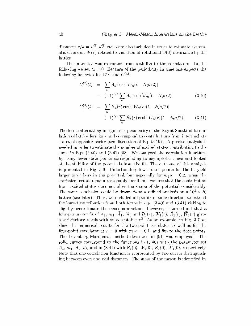
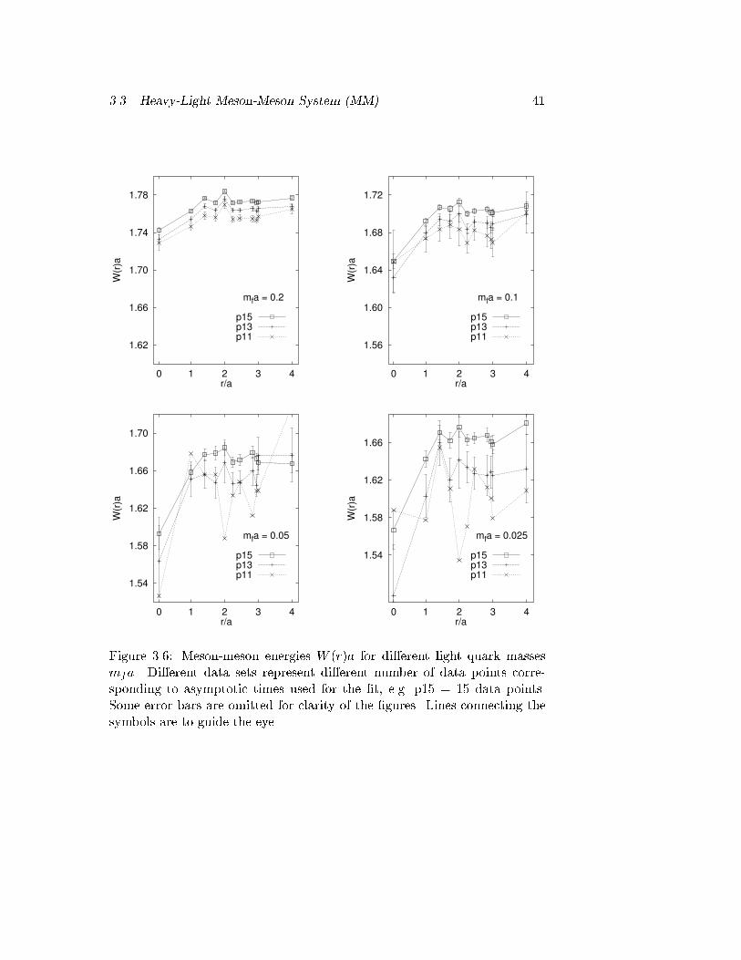
40 Chapter 3. Meson-Meson Interactions on the Latticedistances r=a = p2;p3, etc. were also included in order to estimate system-atic errors on W (r) related to violation of rotational O(3) invariance by thelattice.The potential was extracted from cosh-�ts to the correlators. In thefollowing we set t0 = 0. Because of the periodicity in time one expects thefollowing behavior for C(2) and C(4):C(2)(t) = Xn An cosh [mn(t�Nta=2)]+ (�1)t=aXn eAn cosh [ emn(t�Nta=2)] (3.40)C(4)r (t) = Xn Bn(r) cosh [Wn(r)(t�Nta=2)]+ (�1)t=aXn eBn(r) cosh [fWn(r)(t�Nta=2)]: (3.41)The terms alternating in sign are a peculiarity of the Kogut-Susskind formu-lation of lattice fermions and correspond to contributions from intermediatestates of opposite parity (see discussion of Eq. (3.19)). A precise analysis isneeded in order to estimate the number of excited states contributing to thesums in Eqs. (3.40) and (3.41) [53]. We analyzed the correlation functionsby using fewer data points corresponding to asymptotic times and lookedat the stability of the potentials from the �t. The outcome of this analysisis presented in Fig. 3.6. Unfortunately fewer data points for the �t yieldlarger error bars in the potential, but especially for mfa = 0:2, when thestatistical errors remain reasonably small, one can see that the contributionfrom excited states does not alter the shape of the potential considerably.The same conclusion could be drawn from a re�ned analysis on a 103 � 20lattice (see later). Thus, we included all points in time direction to extractthe lowest contribution from both terms in eqs. (3.40) and (3.41) risking toslightly overestimate the mass parameters. However, it turned out that afour-parameter �t of A1, m1, eA1, em1 and B1(r), W1(r), eB1(r), fW1(r) givesa satisfactory result with an acceptable �2. As an example, in Fig. 3.7 weshow the numerical results for the two-point correlator as well as for thefour-point correlator at r = 0 with mfa = 0:1, and �ts to the data points.The Levenberg-Marquardt method described in [54] was employed. Thesolid curves correspond to the functions in (3.40) with the parameter setA1, m1, eA1, em1 and in (3.41) with B1(0), W1(0), eB1(0), fW1(0), respectively.Note that one correlation function is represented by two curves distinguish-ing between even and odd distances. The mass of the meson is identi�ed by

3.3. Heavy-Light Meson-Meson System (MM) 41

1.62

1.66

1.70

1.74

1.78

0 1 2 3 4

W(r

)a

r/a

mfa = 0.2

p15p13p11

1.56

1.60

1.64

1.68

1.72

0 1 2 3 4

W(r

)a

r/a

mfa = 0.1

p15p13p11

1.54

1.58

1.62

1.66

1.70

0 1 2 3 4

W(r

)a

r/a

mfa = 0.05

p15p13p11

1.54

1.58

1.62

1.66

0 1 2 3 4

W(r

)a

r/a

mfa = 0.025

p15p13p11

Figure 3.6: Meson-meson energies W (r)a for di�erent light quark massesmfa. Di�erent data sets represent di�erent number of data points corre-sponding to asymptotic times used for the �t, e.g. p15 = 15 data points.Some error bars are omitted for clarity of the �gures. Lines connecting thesymbols are to guide the eye.

42 Chapter 3. Meson-Meson Interactions on the Lattice

10-4

10-3

10-2

10-1

0 4 8 12 16

C(2

)

t/a

10-8

10-7

10-6

10-5

10-4

10-3

10-2

10-1

0 4 8 12 16

C(4

)r=

0

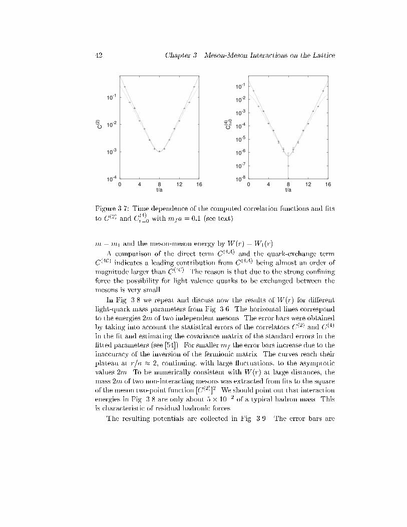
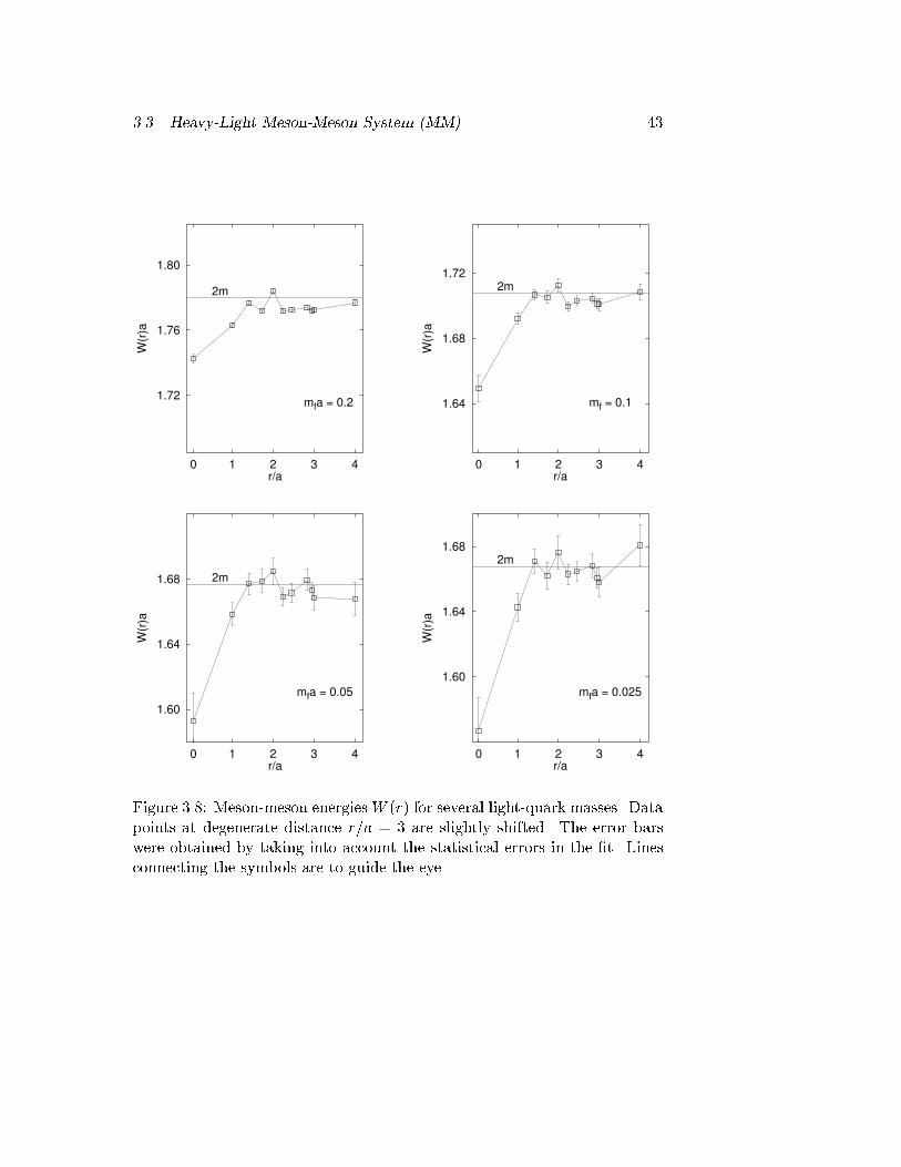
t/aFigure 3.7: Time dependence of the computed correlation functions and �tsto C(2) and C(4)r=0 with mfa = 0:1 (see text).m = m1 and the meson-meson energy by W (r) =W1(r).A comparison of the direct term C(4A) and the quark-exchange termC(4C) indicates a leading contribution from C(4A) being almost an order ofmagnitude larger than C(4C). The reason is that due to the strong con�ningforce the possibility for light valence quarks to be exchanged between themesons is very small.In Fig. 3.8 we repeat and discuss now the results of W (r) for di�erentlight-quark mass parameters from Fig. 3.6. The horizontal lines correspondto the energies 2m of two independent mesons. The error bars were obtainedby taking into account the statistical errors of the correlators C(2) and C(4)in the �t and estimating the covariance matrix of the standard errors in the�tted parameters (see [54]). For smallermf the error bars increase due to theinaccuracy of the inversion of the fermionic matrix. The curves reach theirplateau at r=a � 2, continuing, with large uctuations, to the asymptoticvalues 2m. To be numerically consistent with W (r) at large distances, themass 2m of two non-interacting mesons was extracted from �ts to the squareof the meson two-point function [C(2)]2. We should point out that interactionenergies in Fig. 3.8 are only about 5� 10�2 of a typical hadron mass. Thisis characteristic of residual hadronic forces.The resulting potentials are collected in Fig. 3.9. The error bars are

3.3. Heavy-Light Meson-Meson System (MM) 43

1.72

1.76

1.80

0 1 2 3 4

W(r

)a

r/a

mfa = 0.2

2m

1.64

1.68

1.72

0 1 2 3 4

W(r

)a

r/a

2m

mf = 0.1

1.60

1.64

1.68

0 1 2 3 4

W(r

)a

r/a

2m

mfa = 0.05

1.60

1.64

1.68

0 1 2 3 4

W(r

)a

r/a

2m

mfa = 0.025

Figure 3.8: Meson-meson energiesW (r) for several light-quark masses. Datapoints at degenerate distance r=a = 3 are slightly shifted. The error barswere obtained by taking into account the statistical errors in the �t. Linesconnecting the symbols are to guide the eye.

44 Chapter 3. Meson-Meson Interactions on the Lattice

-0.12

-0.08

-0.04

0.00

0 1 2 3 4

V(r

)a

r/a

mfa

0.2 0.1

0.05 0.025

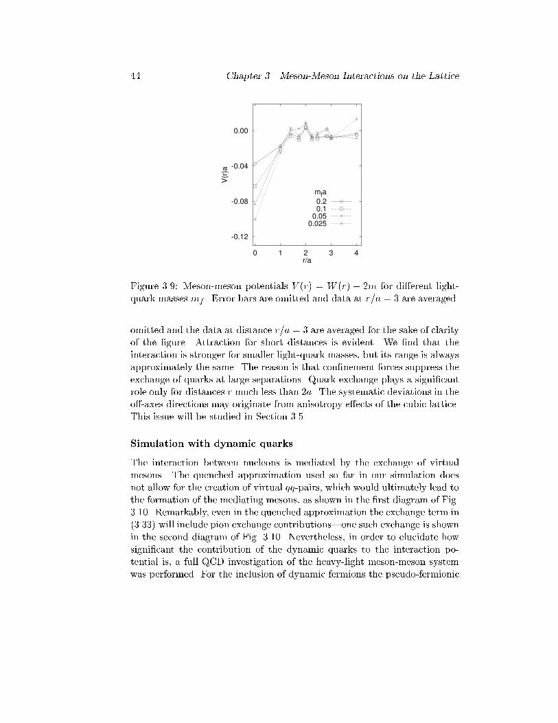
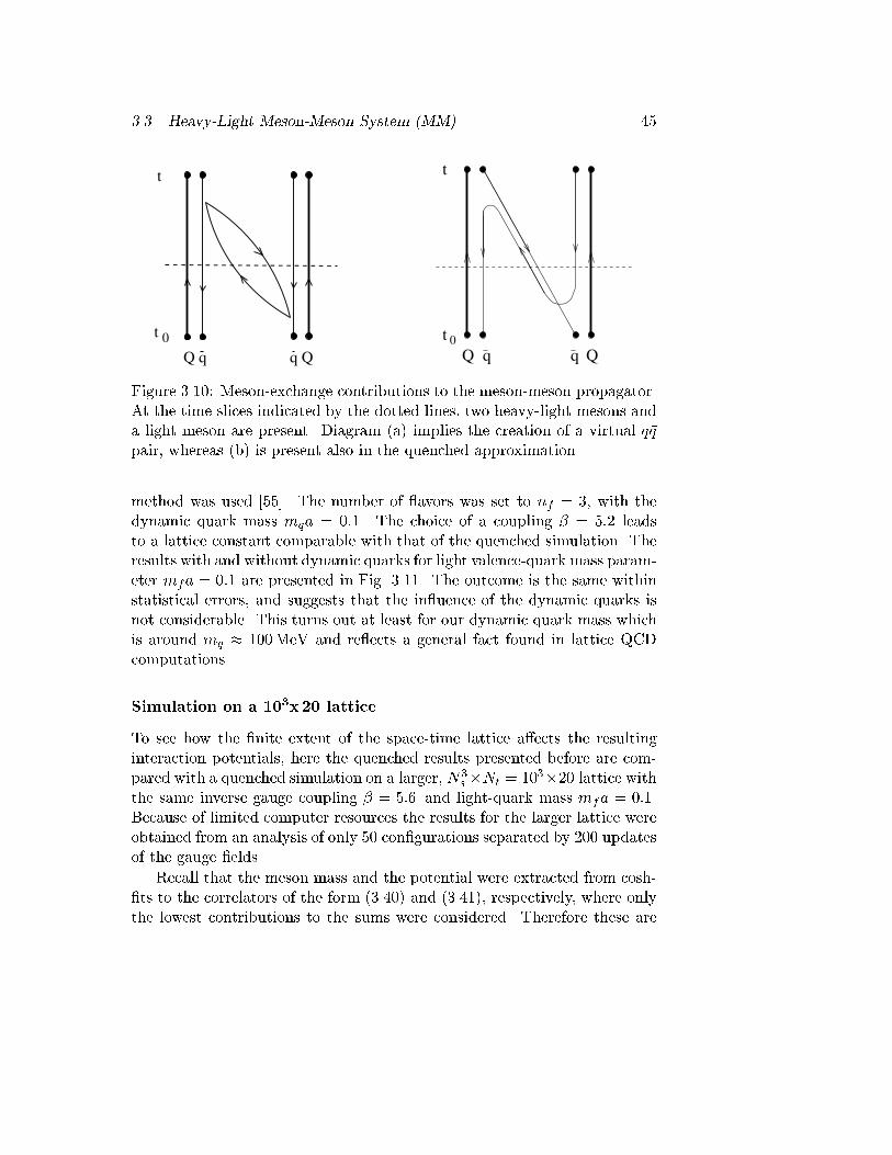
Figure 3.9: Meson-meson potentials V (r) = W (r) � 2m for di�erent light-quark masses mf . Error bars are omitted and data at r=a = 3 are averaged.omitted and the data at distance r=a = 3 are averaged for the sake of clarityof the �gure. Attraction for short distances is evident. We �nd that theinteraction is stronger for smaller light-quark masses, but its range is alwaysapproximately the same. The reason is that con�nement forces suppress theexchange of quarks at large separations. Quark exchange plays a signi�cantrole only for distances r much less than 2a. The systematic deviations in theo�-axes directions may originate from anisotropy e�ects of the cubic lattice.This issue will be studied in Section 3.5.Simulation with dynamic quarksThe interaction between nucleons is mediated by the exchange of virtualmesons. The quenched approximation used so far in our simulation doesnot allow for the creation of virtual q�q-pairs, which would ultimately lead tothe formation of the mediating mesons, as shown in the �rst diagram of Fig.3.10. Remarkably, even in the quenched approximation the exchange term in(3.33) will include pion exchange contributions|one such exchange is shownin the second diagram of Fig. 3.10. Nevertheless, in order to elucidate howsigni�cant the contribution of the dynamic quarks to the interaction po-tential is, a full QCD investigation of the heavy-light meson-meson systemwas performed. For the inclusion of dynamic fermions the pseudo-fermionic

3.3. Heavy-Light Meson-Meson System (MM) 45t

t

Q q

0

q Q

t

Q q Qq

t 0Figure 3.10: Meson-exchange contributions to the meson-meson propagator.At the time slices indicated by the dotted lines, two heavy-light mesons anda light meson are present. Diagram (a) implies the creation of a virtual q�qpair, whereas (b) is present also in the quenched approximation.method was used [55]. The number of avors was set to nf = 3, with thedynamic quark mass mqa = 0:1. The choice of a coupling � = 5:2 leadsto a lattice constant comparable with that of the quenched simulation. Theresults with and without dynamic quarks for light valence-quark mass param-eter mfa = 0:1 are presented in Fig. 3.11. The outcome is the same withinstatistical errors, and suggests that the in uence of the dynamic quarks isnot considerable. This turns out at least for our dynamic quark mass whichis around mq � 100MeV and re ects a general fact found in lattice QCDcomputations.Simulation on a 103x20 latticeTo see how the �nite extent of the space-time lattice a�ects the resultinginteraction potentials, here the quenched results presented before are com-pared with a quenched simulation on a larger, N3s �Nt = 103�20 lattice withthe same inverse gauge coupling � = 5:6 and light-quark mass mfa = 0:1.Because of limited computer resources the results for the larger lattice wereobtained from an analysis of only 50 con�gurations separated by 200 updatesof the gauge �elds.Recall that the meson mass and the potential were extracted from cosh-�ts to the correlators of the form (3.40) and (3.41), respectively, where onlythe lowest contributions to the sums were considered. Therefore these are

46 Chapter 3. Meson-Meson Interactions on the Lattice

-0.08

-0.04

0.00

0 1 2 3 4

V(r

)a

r/a

mfa = 0.1

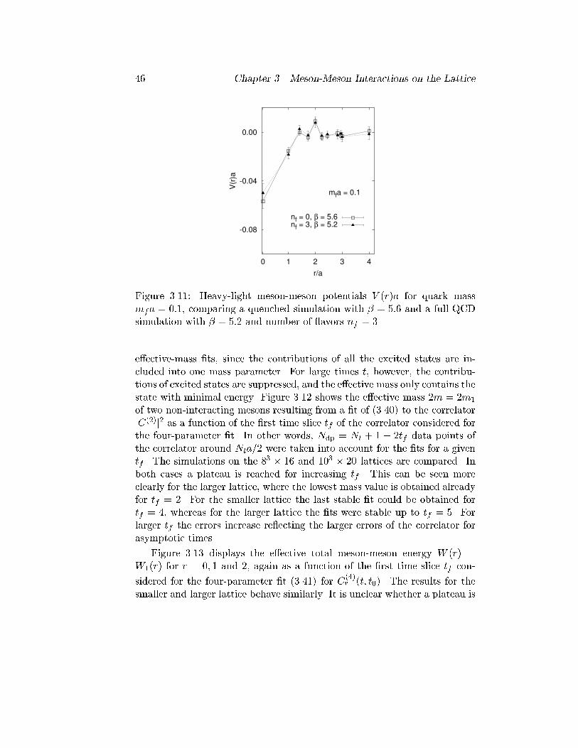
nf = 0, β = 5.6nf = 3, β = 5.2

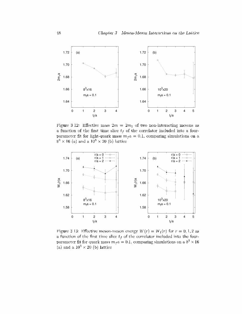
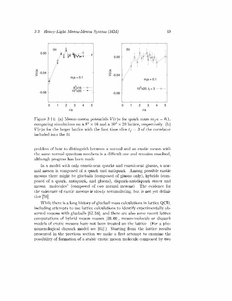
Figure 3.11: Heavy-light meson-meson potentials V (r)a for quark massmfa = 0:1, comparing a quenched simulation with � = 5:6 and a full QCDsimulation with � = 5:2 and number of avors nf = 3.e�ective-mass �ts, since the contributions of all the excited states are in-cluded into one mass parameter. For large times t, however, the contribu-tions of excited states are suppressed, and the e�ective mass only contains thestate with minimal energy. Figure 3.12 shows the e�ective mass 2m = 2m1of two non-interacting mesons resulting from a �t of (3.40) to the correlator[C(2)]2 as a function of the �rst time slice tf of the correlator considered forthe four-parameter �t. In other words, Ndp = Nt + 1 � 2tf data points ofthe correlator around Nta=2 were taken into account for the �ts for a giventf . The simulations on the 83 � 16 and 103 � 20 lattices are compared. Inboth cases a plateau is reached for increasing tf . This can be seen moreclearly for the larger lattice, where the lowest mass value is obtained alreadyfor tf = 2. For the smaller lattice the last stable �t could be obtained fortf = 4, whereas for the larger lattice the �ts were stable up to tf = 5. Forlarger tf the errors increase re ecting the larger errors of the correlator forasymptotic times.Figure 3.13 displays the e�ective total meson-meson energy W (r) =W1(r) for r = 0; 1 and 2, again as a function of the �rst time slice tf con-sidered for the four-parameter �t (3.41) for C(4)r (t; t0). The results for thesmaller and larger lattice behave similarly. It is unclear whether a plateau is

3.3. Heavy-Light Meson-Meson System (MM) 47reached because of the large statistical errors for large tf , but the behaviorof the data points for increasing tf hints at a plateau already at tf = 3.Again, the plateau is approached faster for the larger lattice.The limited volume of the lattice poses an additional problem. Becauseof the periodic boundary conditions the interaction energy can also have con-tributions from the interaction of the meson-meson system with its \mirror"particles. We now consider a �xed hadron that interacts with another hadronseparated by some distance r on the original lattice. The interaction of the�rst hadron with its own mirror particles in the periodic lattices may leadto an additive constant in the potential. If so, changing the spatial extentof the lattice would lead to a change in the resulting interaction potentials.The potentials from the simulations on the two di�erent lattices|with alldata points included into the �ts of the correlators, tf = 1|are presentedin Fig. 3.14. The outcome is the same within statistical errors indicatingthat a spatial volume of 83 is big enough to accommodate the heavy-lightmeson-meson system. This �gure also presents the resulting meson-mesonpotentials from the simulation on the larger lattice with the �rst time slicetf = 3 of the correlator considered for the four-parameter �t. Here thecontributions from excited states are at least partly eliminated. Comparingwith the tf = 1 results one can see that the shape of the potential remainsstable. This is a hint that also for lattices with larger time extents, wherethe extraction of the ground state becomes feasible, the qualitative behaviorof the potential may be the same. This result also suggests that the excitedstates of the four-quark system are not resonant states of the meson-mesonsystem but rather excitations within the individual mesons.3.3.5 Exotic Mesons as Two-Meson \Molecules"An exotic meson has a structure which is di�erent from that of a normalmeson. A normal meson has the quantum numbers of a possible boundstate of a quark and an antiquark: so-called normal quantum numbers. Ameson which does not have normal quantum numbers is said to have exoticquantum numbers, and is by de�nition exotic. Some physicists think thatmesons with exotic quantum numbers ought to exist because QCD does notobviously forbid them, but there is not yet de�nitive experimental evidencefor the existence of any such meson.A meson may have normal quantum numbers and still be exotic if itsinternal structure di�ers from that of a normal meson. Although there arecandidates for such exotics, none has yet been positively identi�ed. The

48 Chapter 3. Meson-Meson Interactions on the Lattice

1.64

1.66

1.68

1.70

1.72

0 1 2 3 4

2m

1a

tf/a

mfa = 0.1

83x16

(a)

1.64

1.66

1.68

1.70

1.72

0 1 2 3 4 5

2m

1a

tf/a

mfa = 0.1

103x20

(b)

Figure 3.12: E�ective mass 2m = 2m1 of two non-interacting mesons asa function of the �rst time slice tf of the correlator included into a four-parameter �t for light-quark mass mfa = 0:1, comparing simulations on a83 � 16 (a) and a 103 � 20 (b) lattice.

1.58

1.62

1.66

1.70

1.74

0 1 2 3 4

W1(r

)a

tf/a

mfa = 0.1

83x16

(a)r/a = 0r/a = 1r/a = 2

1.58

1.62

1.66

1.70

1.74

0 1 2 3 4 5

W1(r

)a

tf/a

mfa = 0.1

103x20

(b)r/a = 0r/a = 1r/a = 2

Figure 3.13: E�ective meson-meson energy W (r) = W1(r) for r = 0; 1; 2 asa function of the �rst time slice tf of the correlator included into the four-parameter �t for quark mass mfa = 0:1, comparing simulations on a 83�16(a) and a 103 � 20 (b) lattice.

3.3. Heavy-Light Meson-Meson System (MM) 49

-0.08

-0.04

0.00

0 1 2 3 4 5

V(r

)a

r/a

mfa = 0.1

(a)

83x16

103x20

-0.08

-0.04

0.00

0 1 2 3 4 5

V(r

)ar/a

mfa = 0.1

(b)

103x20, tf = 3

Figure 3.14: (a) Meson-meson potentials V (r)a for quark mass mfa = 0:1,comparing simulations on a 83 � 16 and a 103 � 20 lattice, respectively. (b)V (r)a for the larger lattice with the �rst time slice tf = 3 of the correlatorincluded into the �t.problem of how to distinguish between a normal and an exotic meson withthe same normal quantum numbers is a di�cult one and remains unsolved,although progress has been made.In a model with only constituent quarks and constituent gluons, a nor-mal meson is composed of a quark and antiquark. Among possible exoticmesons there might be glueballs (composed of gluons only), hybrids (com-posed of a quark, antiquark, and gluons), diquark-antidiquark states andmeson \molecules" (composed of two normal mesons). The evidence forthe existence of exotic mesons is slowly accumulating, but is not yet de�ni-tive [56].While there is a long history of glueball mass calculations in lattice QCD,including attempts to use lattice calculations to identify experimentally ob-served mesons with glueballs [57, 58], and there are also some recent latticecomputations of hybrid meson masses [59, 60], meson-molecule or diquarkmodels of exotic mesons have not been treated on the lattice. (For a phe-nomenological diquark model see [61].) Starting from the lattice resultspresented in the previous section we make a �rst attempt to examine thepossibility of formation of a stable exotic meson molecule composed by two

50 Chapter 3. Meson-Meson Interactions on the Latticeheavy-light mesons.First we determine the quantum numbers of our four-quark system. Inthe isospin representation we have �II3 = � 12� 12 for the heavy-light meson�elds in (3.20) and therefore the two-meson system de�ned by (3.21) formsan I = 1, I3 = �1 state. For the case of two mesons of an isospin doublet,de�ned by the �eld�~r(t) = (p2V )�1X~x X~y �~r;~y�~x h� 12+ 12 (~xt)� 12� 12 (~yt) + � 12� 12 (~xt)� 12+ 12 (~yt)i ;(3.42)one has a I = 1, I3 = 0 state. Replacing the �eld (3.42) into the de�ning for-mula of the four-point correlator (3.23) yields again (3.33) in the heavy-lightapproximation, provided that the light (u and d) quark masses are degener-ate. Thus the MM states corresponding to di�erent I3s are approximatelyidentical. When computing the four-point correlators we sum over all spa-tial directions, therefore we project into the s-wave part of the correlators,describing a state with JP = 0+.Lattice computations are easier for large quark masses (see Section 3.1.1).The light-quark masses used in our simulations are in the range mf �25� 200MeV which is much greater than the mass of a u or d quark. Sinceneither the full QCD simulation nor the simulation on the larger lattice ledto substantial changes of the results, we took the data from the original run(Fig. 3.9) for this investigation. In this way we could make an extrapolationof the data for di�erent quark masses towards the chiral limit, getting closerto the masses of the light physical quarks. By a two-parameter �t to theresulting data points using a Gaussian function we obtained an analytic formfor the meson-meson interaction potential which is shown in Figs. 3.15(a).The interaction potential was then used as an input to the Schr�odinger equa-tion for a phase shift calculation. The resulting phase shifts are displayed inFig. 3.15(b) with a variation in the meson mass. The extrapolated mesonmass reads ma = 0:83 .Although the potential is attractive, the computed phase shifts signalthe absence of a bound state. For a decisive check, the meson mass and theinteraction potential were used as an input for a resonant state searchingprogram presented in [62]. Neither bound nor resonant meson-meson stateswere found. This is in agreement with the predictions of most of the phe-nomenological models. Whether such exotic mesons exists or not has to beanswered by future experiments.

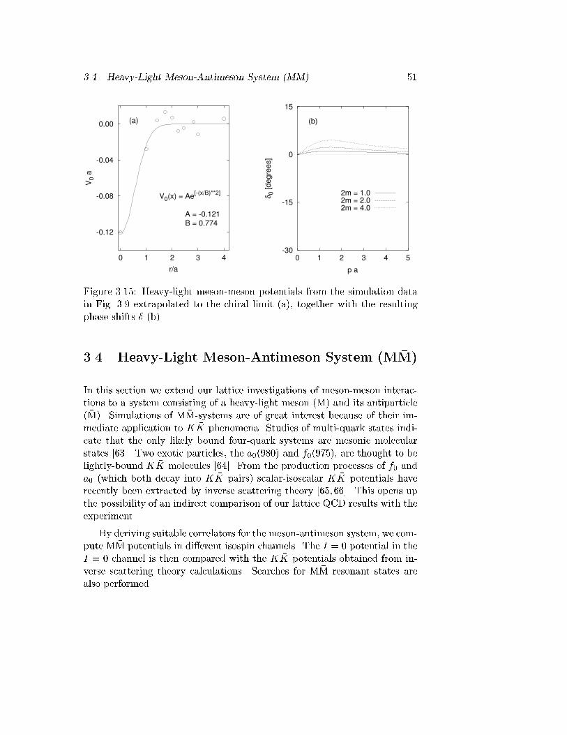
3.4. Heavy-Light Meson-Antimeson System (M �M) 51

-0.12

-0.08

-0.04

0.00

0 1 2 3 4

V0 a

r/a

V0(x) = Ae[-(x/B)**2]

A = -0.121B = 0.774

(a)

-30

-15

0

15

0 1 2 3 4 5

δ0 [degre

es]

p a

(b)

2m = 1.02m = 2.02m = 4.0

Figure 3.15: Heavy-light meson-meson potentials from the simulation datain Fig. 3.9 extrapolated to the chiral limit (a), together with the resultingphase shifts � (b).3.4 Heavy-Light Meson-Antimeson System (M �M)In this section we extend our lattice investigations of meson-meson interac-tions to a system consisting of a heavy-light meson (M) and its antiparticle( �M). Simulations of M �M-systems are of great interest because of their im-mediate application to K �K phenomena. Studies of multi-quark states indi-cate that the only likely bound four-quark systems are mesonic molecularstates [63]. Two exotic particles, the a0(980) and f0(975), are thought to belightly-bound K �K molecules [64]. From the production processes of f0 anda0 (which both decay into K �K pairs) scalar-isoscalar K �K potentials haverecently been extracted by inverse scattering theory [65, 66]. This opens upthe possibility of an indirect comparison of our lattice QCD results with theexperiment.By deriving suitable correlators for the meson-antimeson system, we com-pute M �M potentials in di�erent isospin channels. The I = 0 potential in theI = 0 channel is then compared with the K �K potentials obtained from in-verse scattering theory calculations. Searches for M �M resonant states arealso performed.

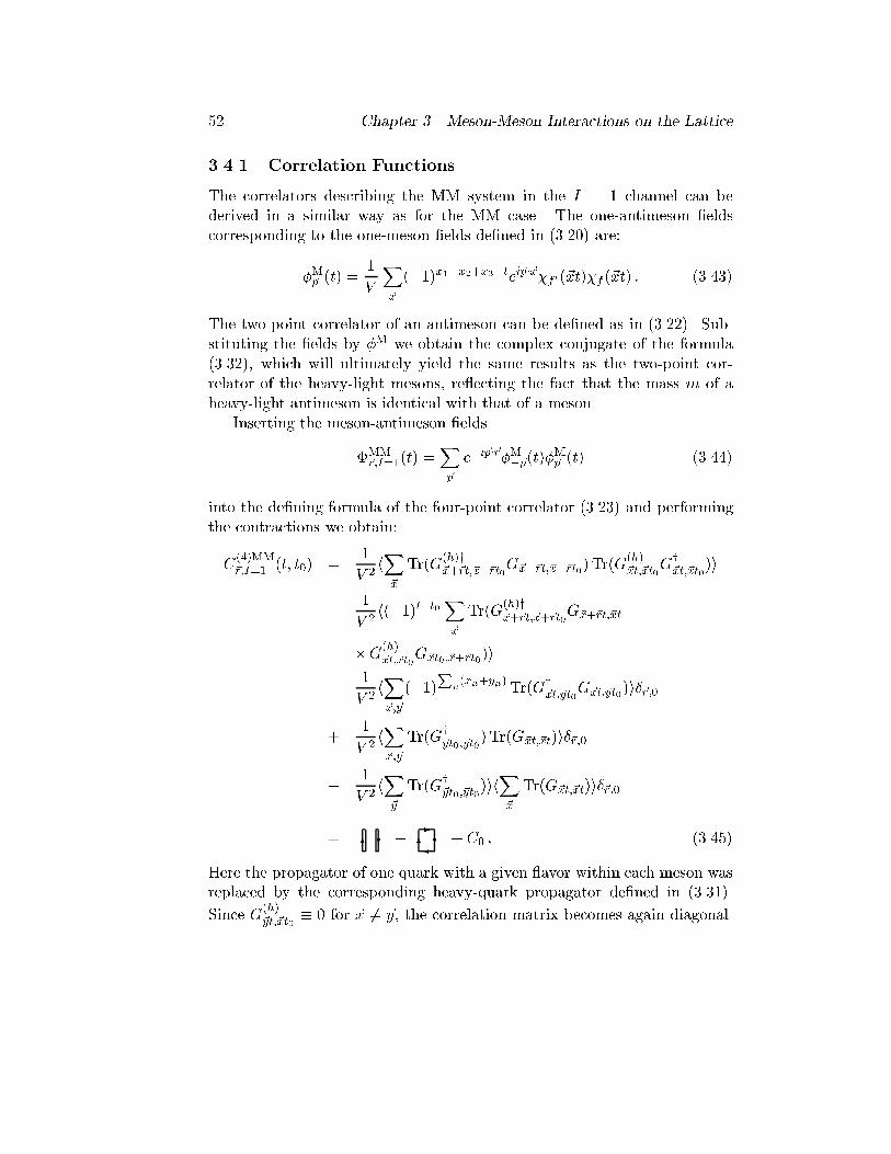
52 Chapter 3. Meson-Meson Interactions on the Lattice3.4.1 Correlation FunctionsThe correlators describing the M �M system in the I = 1 channel can bederived in a similar way as for the MM case. The one-antimeson �eldscorresponding to the one-meson �elds de�ned in (3.20) are:� �M~p (t) = 1V X~x (�1)x1+x2+x3+tei~p�~x ��f 0(~xt)�f (~xt) : (3.43)The two-point correlator of an antimeson can be de�ned as in (3.22). Sub-stituting the �elds by � �M we obtain the complex conjugate of the formula(3.32), which will ultimately yield the same results as the two-point cor-relator of the heavy-light mesons, re ecting the fact that the mass m of aheavy-light antimeson is identical with that of a meson.Inserting the meson-antimeson �elds�M�M~r;I=1(t) =X~p e�i~p�~r�M�~p(t)� �M~p (t) (3.44)into the de�ning formula of the four-point correlator (3.23) and performingthe contractions we obtain:C(4)M �M~r;I=1 (t; t0) = 1V 2 hX~x Tr(G(h)y~x+~rt;~x+~rt0G~x+~rt;~x+~rt0)Tr(G(h)~xt;~xt0Gy~xt;~xt0)i� 1V 2 h(�1)t+t0 X~x Tr(G(h)y~x+~rt;~x+~rt0G~x+~rt;~xt�G(h)~xt;~xt0G~xt0;~x+~rt0)i� 1V 2 hX~x;~y (�1)P�(x�+y�) Tr(Gy~xt;~yt0G~xt;~yt0)i�~r;0+ 1V 2 hX~x;~y Tr(Gy~yt0;~yt0)Tr(G~xt;~xt)i�~r;0� 1V 2 hX~y Tr(Gy~yt0;~yt0)ihX~x Tr(G~xt;~xt)i�~r;0= 6?� 6-�?+ C0 : (3.45)Here the propagator of one quark with a given avor within each meson wasreplaced by the corresponding heavy-quark propagator de�ned in (3.31).Since G(h)~yt;~xt0 � 0 for ~x 6= ~y, the correlation matrix becomes again diagonal.

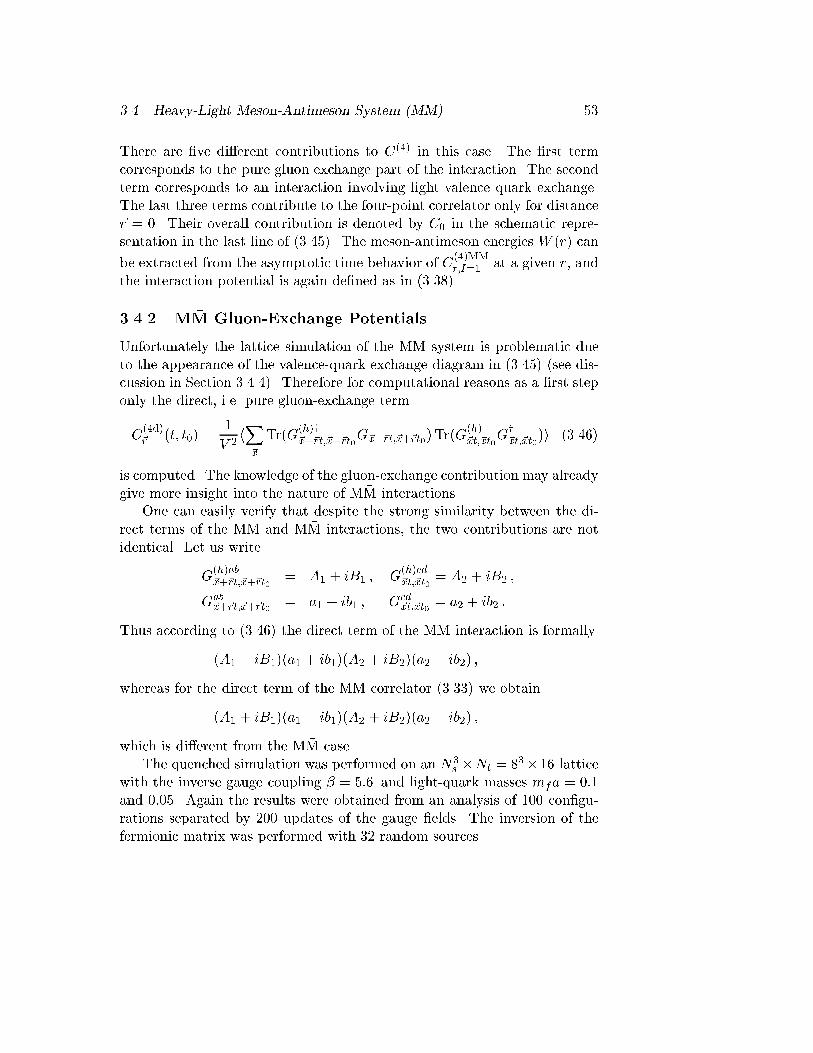
3.4. Heavy-Light Meson-Antimeson System (M �M) 53There are �ve di�erent contributions to C(4) in this case. The �rst termcorresponds to the pure gluon exchange part of the interaction. The secondterm corresponds to an interaction involving light valence quark exchange.The last three terms contribute to the four-point correlator only for distance~r = 0. Their overall contribution is denoted by C0 in the schematic repre-sentation in the last line of (3.45). The meson-antimeson energies W (r) canbe extracted from the asymptotic time behavior of C(4)M �Mr;I=1 at a given r, andthe interaction potential is again de�ned as in (3.38).3.4.2 M �M Gluon-Exchange PotentialsUnfortunately the lattice simulation of the M �M system is problematic dueto the appearance of the valence-quark exchange diagram in (3.45) (see dis-cussion in Section 3.4.4). Therefore for computational reasons as a �rst steponly the direct, i.e. pure gluon-exchange termC(4d)~r (t; t0) = 1V 2 hX~x Tr(G(h)y~x+~rt;~x+~rt0G~x+~rt;~x+~rt0)Tr(G(h)~xt;~xt0Gy~xt;~xt0)i (3.46)is computed. The knowledge of the gluon-exchange contribution may alreadygive more insight into the nature of M �M interactions.One can easily verify that despite the strong similarity between the di-rect terms of the MM and M �M interactions, the two contributions are notidentical. Let us writeG(h)ab~x+~rt;~x+~rt0 = A1 + iB1 ; G(h)cd~xt;~xt0 = A2 + iB2 ;Gab~x+~rt;~x+~rt0 = a1 + ib1 ; Gcd~xt;~xt0 = a2 + ib2 :Thus according to (3.46) the direct term of the M �M interaction is formally(A1 � iB1)(a1 + ib1)(A2 + iB2)(a2 � ib2) ;whereas for the direct term of the MM correlator (3.33) we obtain(A1 + iB1)(a1 � ib1)(A2 + iB2)(a2 � ib2) ;which is di�erent from the M �M case.The quenched simulation was performed on an N3s �Nt = 83�16 latticewith the inverse gauge coupling � = 5:6 and light-quark masses mfa = 0:1and 0:05. Again the results were obtained from an analysis of 100 con�gu-rations separated by 200 updates of the gauge �elds. The inversion of thefermionic matrix was performed with 32 random sources.

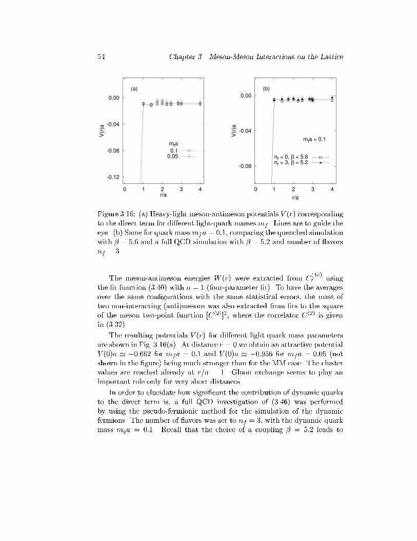
54 Chapter 3. Meson-Meson Interactions on the Lattice

-0.12

-0.08

-0.04

0.00

0 1 2 3 4

V(r

)a

r/a

mfa

(a)

0.1 0.05

-0.08

-0.04

0.00

0 1 2 3 4

V(r

)a

r/a

mfa = 0.1

(b)

nf = 0, β = 5.6 nf = 3, β = 5.2

Figure 3.16: (a) Heavy-light meson-antimeson potentials V (r) correspondingto the direct term for di�erent light-quark massesmf . Lines are to guide theeye. (b) Same for quark massmfa = 0:1, comparing the quenched simulationwith � = 5:6 and a full QCD simulation with � = 5:2 and number of avorsnf = 3.The meson-antimeson energies W (r) were extracted from C(4d)r usingthe �t function (3.40) with n = 1 (four-parameter �t). To have the averagesover the same con�gurations with the same statistical errors, the mass oftwo non-interacting (anti)mesons was also extracted from �ts to the squareof the meson two-point function [C(2)]2, where the correlator C(2) is givenin (3.32).The resulting potentials V (r) for di�erent light-quark mass parametersare shown in Fig. 3.16(a). At distance r = 0 we obtain an attractive potentialV (0)a ' �0:662 for mfa = 0:1 and V (0)a ' �0:956 for mfa = 0:05 (notshown in the �gure) being much stronger than for the MM case. The clustervalues are reached already at r=a = 1. Gluon exchange seems to play animportant role only for very short distances.In order to elucidate how signi�cant the contribution of dynamic quarksto the direct term is, a full QCD investigation of (3.46) was performedby using the pseudo-fermionic method for the simulation of the dynamicfermions. The number of avors was set to nf = 3, with the dynamic quarkmass mqa = 0:1. Recall that the choice of a coupling � = 5:2 leads to

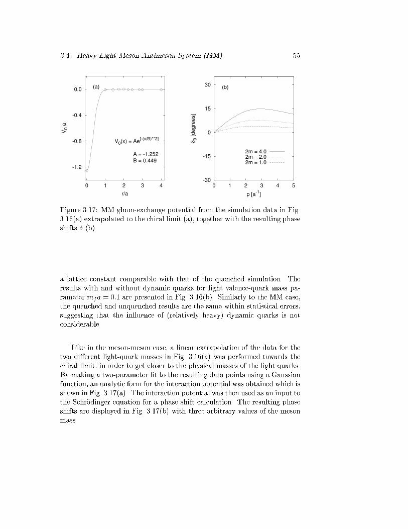
3.4. Heavy-Light Meson-Antimeson System (M �M) 55

-1.2

-0.8

-0.4

0.0

0 1 2 3 4

V0 a

r/a

V0(x) = Ae[-(x/B)**2]

A = -1.252B = 0.449

(a)

-30

-15

0

15

30

0 1 2 3 4 5

δ0 [degre

es]

p [a-1

]

(b)

2m = 4.02m = 2.02m = 1.0

Figure 3.17: M �M gluon-exchange potential from the simulation data in Fig.3.16(a) extrapolated to the chiral limit (a), together with the resulting phaseshifts � (b).a lattice constant comparable with that of the quenched simulation. Theresults with and without dynamic quarks for light valence-quark mass pa-rameter mfa = 0:1 are presented in Fig. 3.16(b). Similarly to the MM case,the quenched and unquenched results are the same within statistical errors,suggesting that the in uence of (relatively heavy) dynamic quarks is notconsiderable.Like in the meson-meson case, a linear extrapolation of the data for thetwo di�erent light-quark masses in Fig. 3.16(a) was performed towards thechiral limit, in order to get closer to the physical masses of the light quarks.By making a two-parameter �t to the resulting data points using a Gaussianfunction, an analytic form for the interaction potential was obtained which isshown in Fig. 3.17(a). The interaction potential was then used as an input tothe Schr�odinger equation for a phase shift calculation. The resulting phaseshifts are displayed in Fig. 3.17(b) with three arbitrary values of the mesonmass.

56 Chapter 3. Meson-Meson Interactions on the Lattice3.4.3 I = 0 M �M-Potentials from Lattice and Inverse Scatter-ingA desirable next step in our program would be to compare our lattice QCDresults with the experiment. Unfortunately the interactions between mesonshaving one heavy avor are known very poorly. Our knowledge of the meson-meson interactions is based mainly on reactions in which ��� or K �K pairs areproduced. The production processes of the scalar mesons f0 and a0 (whichboth decay into K �K pairs) have been studied in many experiments [67,68].From the analysis of the experimental data information about K �K scalar-isoscalar phase shifts has been extracted [69].To make a comparison with our M �M potentials, in principle one has toobtain a simple potential operator VL(r) from experimentally known phaseshifts �L(k) for a given equation of motion. Such an operator may be calcu-lated by inverse scattering theory [70, 71].Because the experimental information is limited to a certain energy in-terval, the inverse problem is ill-posed and one has to regularize it, i.e. onehas to interpolate and extrapolate the phase shifts for all energies in thesmoothest possible way, obeying the proper behavior at low and highest en-ergies. Thus any meaningful application of the potential obtained in thisway is limited to a domain where genuine data are used.The experimental situation for low energy K �K scattering was paramet-rized with an e�ective range expansion by Kaminski and Lesniak [72]. Theirexpansion is valid at low energy and, unfortunately, takes inelasticities notinto account. Nevertheless it is the only available experimental informationused in an inversion scheme, and since also in the lattice QCD case noinelastic channels are considered, a comparison of the results is interesting.Kaminski and Lesniak [72] give two sets of parameters for the e�ectiverange expansionk cot �K(k) = 1Re aK + 12RKk2 + VKk4 +O(k6) ; (3.47)which are documented in Table 3.1. Based on these parameters, Sanderand von Geramb [65,66] calculated the phase shifts �0(MK �K) shown in Fig.3.18(b). These phase shifts were then used as input for a standard rationalGelfand{Levitan{Marchenko inversion program [70, 71].The real local and energy independent inversion potentials are describingpurely elastic K �K scattering. Coulomb e�ects are not included. The resultis shown in Fig. 3.18(a). The reproduction of the e�ective range parameters

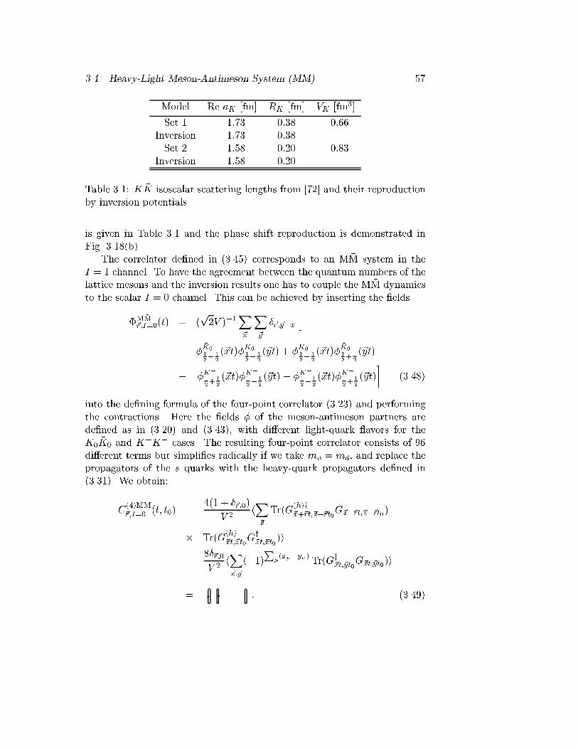
3.4. Heavy-Light Meson-Antimeson System (M �M) 57Model Re aK [fm] RK [fm] VK [fm3]Set 1 �1:73 0:38 �0:66Inversion �1:73 0:38Set 2 �1:58 0:20 �0:83Inversion �1:58 0:20Table 3.1: K �K isoscalar scattering lengths from [72] and their reproductionby inversion potentials.is given in Table 3.1 and the phase shift reproduction is demonstrated inFig. 3.18(b).The correlator de�ned in (3.45) corresponds to an M �M system in theI = 1 channel. To have the agreement between the quantum numbers of thelattice mesons and the inversion results one has to couple the M �M dynamicsto the scalar I = 0 channel. This can be achieved by inserting the �elds�M�M~r;I=0(t) = (p2V )�1X~x X~y �~r;~y�~x h� �K012+ 12 (~xt)�K012� 12 (~yt) + �K012� 12 (~xt)� �K012+ 12 (~yt)� �K+12+ 12 (~xt)�K�12� 12 (~yt)� �K�12� 12 (~xt)�K+12+ 12 (~yt)� (3.48)into the de�ning formula of the four-point correlator (3.23) and performingthe contractions. Here the �elds � of the meson-antimeson partners arede�ned as in (3.20) and (3.43), with di�erent light-quark avors for theK0 �K0 and K+K� cases. The resulting four-point correlator consists of 96di�erent terms but simpli�es radically if we take mu = md, and replace thepropagators of the s quarks with the heavy-quark propagators de�ned in(3.31). We obtain:C(4)M �M~r;I=0 (t; t0) = 4(1 + �~r;0)V 2 hX~x Tr(G(h)y~x+~rt;~x+~rt0G~x+~rt;~x+~rt0)� Tr(G(h)~xt;~xt0Gy~xt;~xt0)i� 8�~r;0V 2 hX~x;~y (�1)P�(x�+y�) Tr(Gy~xt;~yt0G~xt;~yt0)i= 6?� : (3.49)

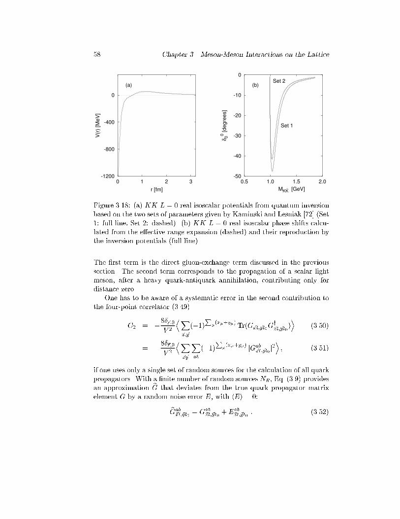
58 Chapter 3. Meson-Meson Interactions on the Lattice

-1200

-800

-400

0

0 1 2 3

V(r

) [M

eV

]

r [fm]

(a)

-50

-40

-30

-20

-10

0

0.5 1.0 1.5 2.0

δ00 [degre

es]

MKK- [GeV]

Set 1

Set 2(b)

Figure 3.18: (a) K �K L = 0 real isoscalar potentials from quantum inversionbased on the two sets of parameters given by Kaminski and Lesniak [72] (Set1: full line, Set 2: dashed). (b) K �K L = 0 real isoscalar phase shifts calcu-lated from the e�ective range expansion (dashed) and their reproduction bythe inversion potentials (full line).The �rst term is the direct gluon-exchange term discussed in the previoussection. The second term corresponds to the propagation of a scalar lightmeson, after a heavy quark-antiquark annihilation, contributing only fordistance zero.One has to be aware of a systematic error in the second contribution tothe four-point correlator (3.49)C2 = �8�~r;0V 2 DX~x;~y (�1)P�(x�+y�) Tr(G~xt;~yt0Gy~xt;~yt0)E (3.50)= �8�~r;0V 2 DX~x~y Xab (�1)P�(x�+y�) jGab~xt;~yt0 j2E ; (3.51)if one uses only a single set of random sources for the calculation of all quarkpropagators. With a �nite number of random sources NR, Eq. (3.9) providesan approximation eG that deviates from the true quark propagator matrixelement G by a random noise error E, with hEi = 0:eGab~xt;~yt0 = Gab~xt;~yt0 +Eab~xt;~yt0 : (3.52)

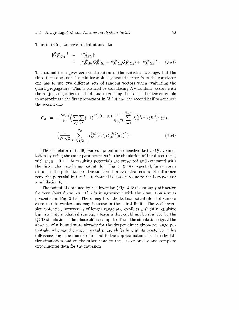
3.4. Heavy-Light Meson-Antimeson System (M �M) 59Thus in (3.51) we have contributions likej eGab~xt;~yt0 j2 = jGab~xt;~yt0 j2+ (Eab~xt;~yt0Gab�~xt;~yt0 +Eab�~xt;~yt0Gab~xt;~yt0) + jEab~xt;~yt0 j2 : (3.53)The second term gives zero contribution in the statistical average, but thethird term does not. To eliminate this systematic error from the correlatorone has to use two di�erent sets of random vectors when evaluating thequark propagators. This is realized by calculating NR random vectors withthe conjugate gradient method, and then using the �rst half of the ensembleto approximate the �rst propagator in (3.50) and the second half to generatethe second oneC2 = �8�~r;0V 2 DX~x~y Xab (�1)P�(x�+y�) 1NR=2 NR=2Xi=1 I(t0)i;a (~x; t)R�(t0)i;b (~y ) �� 1NR=2 NRXj=NR=2+1 I(t0)j;a (~x; t)R�(t0)j;b (~y )��E : (3.54)The correlator in (3.49) was computed in a quenched lattice QCD simu-lation by using the same parameters as in the simulation of the direct term,with mfa = 0:1. The resulting potentials are presented and compared withthe direct gluon-exchange potentials in Fig. 3.19. As expected, for non-zerodistances the potentials are the same within statistical errors. For distancezero, the potential in the I = 0 channel is less deep due to the heavy-quarkannihilation term.The potential obtained by the inversion (Fig. 3.18) is strongly attractivefor very short distances. This is in agreement with the simulation resultspresented in Fig. 3.19. The strength of the lattice potentials at distancesclose to 0 is weaker but may increase in the chiral limit. The K �K inver-sion potential, however, is of longer range and exhibits a slightly repulsivebump at intermediate distances, a feature that could not be resolved by theQCD simulation. The phase shifts computed from the simulation signal theabsence of a bound state already for the deeper direct gluon-exchange po-tentials, whereas the experimental phase shifts hint at its existence. Thisdi�erence might be due on one hand to the approximations used in the lat-tice simulation and on the other hand to the lack of precise and completeexperimental data for the inversion.

60 Chapter 3. Meson-Meson Interactions on the Lattice

-0.6

-0.4

-0.2

0.0

0 1 2 3 4

V(r

)a

r/a

mfa = 0.1

I = 0gl.exch.

Figure 3.19: M �M potential in the I = 0 channel for light-quark mass mfa =0:1, compared to the direct gluon-exchange potential for the same mf fromFig. 3.16(a).3.4.4 I = 1 M �M-PotentialsThe four-point correlator describing the dynamics of the I = 1 M �M systemis given in (3.45). The lattice simulation of this correlator requires higherCPU time due to new technical solutions in the computation of the valence-quark exchange diagram. In order to evaluate this term one has to computequark propagators of the type G(t; t). With the random source techniqueused by us only propagators of the type G(t; t0) are obtained, with �xed t0(see Section 3.1.1). Thus in order to get all possible propagators G(t; t) inprinciple one has to perform the fermionic matrix inversionNt times by usingin (3.3) Nt di�erent sets of sources of the type (3.5) which are successivelynon-zero on di�erent time slices t0 2 f1; : : : ; Ntg . Regarding the cost of thesimulation this means an Nt-fold increase in CPU time.In principle all-to-all propagators can be obtained also by replacing thesources (3.5) by sources that are non-zero on all time slicesYi;a(~x; x4) = Ri;a(~x; x4) ; (3.55)

3.4. Heavy-Light Meson-Antimeson System (M �M) 61where the complex random vectors R satisfy the relation1NR NRXi=1R�i;a(~x; x4)Ri;b(~y; y4) = �~x;~y �x4;y4�a;b : (3.56)With this choice of random sources, however, one does not impose an exactdelta function for the time coordinate, as a result of which the exponentialfall-o� in time of the correlators will be a�ected, causing di�culties in theextraction of interaction potentials. Note that all propagators which donot have the form G(t; t0) are of the type G(t; t), i.e. start and end onthe same time slice t. This observation may help in the evaluation of thevalence-quark exchange diagram. A plausible trick which comes to mind isto determine the propagators G(t; t0)|which ultimately determine the fall-o� of the correlators|in the usual way, and to use the sources (3.55) in asubsequent inversion of the fermionic matrix to determine the propagatorsG(t; t). Such a procedure means only a two-fold increase in CPU time, andthus a remarkable improvement compared to the other method.The correlator in (3.45) was computed in quenched lattice QCD with thesame parameters as in the previous simulations. All �ve terms were takeninto account. The light-quark propagators were calculated by both methodspresented above. In the case with Nt = 16 sets of random sources only 50con�gurations were generated because of the huge CPU demand. The re-sulting interaction potentials are presented in Fig. 3.20. The two di�erentmethods yield the same results within statistical errors. The potential isattractive for r=a = 1, whereas for larger separations the interaction is com-patible with zero. A comparison with the gluon-exchange potentials from thedirect diagram in Fig. 3.16 shows that the valence-quark exchange diagramyields an attraction of longer range. This term includes pion-exchange con-tributions even in the quenched approximation as demonstrated in Fig. 3.21.The big error bars at distance r = 0 are a consequence of the accumulationof the uncertainties of the �ve di�erent terms contributing to C(4)M �Mr=0;I=1.Comparing Figs. 3.20 and 3.9 it turns out that the I = 1 M �M poten-tials are approximately of the same range as the I = 1 MM potentials, butthey are much more attractive. In order to examine the possibility of theformation of bound M �M states, a further quantum-mechanical analysis isdesirable. Such an analysis requires an analytic form for the interaction po-tential. Obviously, the strength of the potential at r = 0 is decisive for thedetermination of such an analytic form and ultimately for the existence ornon-existence of a bound resonant state. Because of the large uncertainty

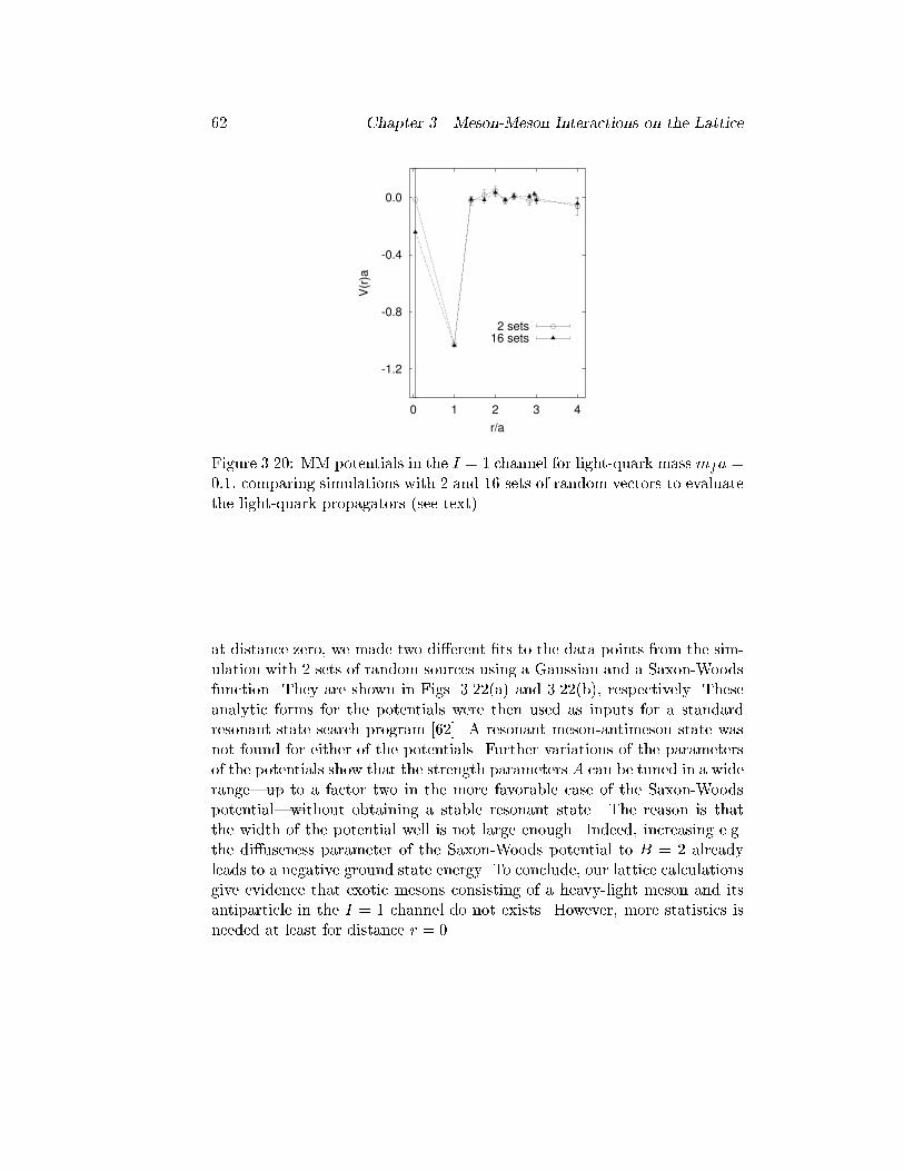
62 Chapter 3. Meson-Meson Interactions on the Lattice

-1.2

-0.8

-0.4

0.0

0 1 2 3 4

V(r

)a

r/a

2 sets16 sets

Figure 3.20: M �M potentials in the I = 1 channel for light-quark massmfa =0:1, comparing simulations with 2 and 16 sets of random vectors to evaluatethe light-quark propagators (see text).at distance zero, we made two di�erent �ts to the data points from the sim-ulation with 2 sets of random sources using a Gaussian and a Saxon-Woodsfunction. They are shown in Figs. 3.22(a) and 3.22(b), respectively. Theseanalytic forms for the potentials were then used as inputs for a standardresonant state search program [62]. A resonant meson-antimeson state wasnot found for either of the potentials. Further variations of the parametersof the potentials show that the strength parameters A can be tuned in a widerange|up to a factor two in the more favorable case of the Saxon-Woodspotential|without obtaining a stable resonant state. The reason is thatthe width of the potential well is not large enough. Indeed, increasing e.g.the di�useness parameter of the Saxon-Woods potential to B = 2 alreadyleads to a negative ground state energy. To conclude, our lattice calculationsgive evidence that exotic mesons consisting of a heavy-light meson and itsantiparticle in the I = 1 channel do not exists. However, more statistics isneeded at least for distance r = 0.

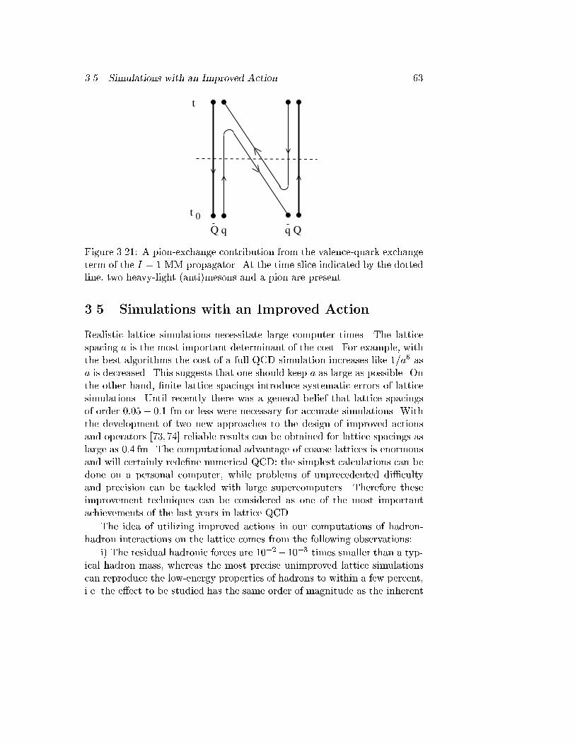
3.5. Simulations with an Improved Action 63t

0t

q QQ qFigure 3.21: A pion-exchange contribution from the valence-quark exchangeterm of the I = 1 M �M propagator. At the time slice indicated by the dottedline, two heavy-light (anti)mesons and a pion are present.3.5 Simulations with an Improved ActionRealistic lattice simulations necessitate large computer times. The latticespacing a is the most important determinant of the cost. For example, withthe best algorithms the cost of a full QCD simulation increases like 1=a6 asa is decreased. This suggests that one should keep a as large as possible. Onthe other hand, �nite lattice spacings introduce systematic errors of latticesimulations. Until recently there was a general belief that lattice spacingsof order 0:05� 0:1 fm or less were necessary for accurate simulations. Withthe development of two new approaches to the design of improved actionsand operators [73,74] reliable results can be obtained for lattice spacings aslarge as 0:4 fm. The computational advantage of coarse lattices is enormousand will certainly rede�ne numerical QCD: the simplest calculations can bedone on a personal computer, while problems of unprecedented di�cultyand precision can be tackled with large supercomputers. Therefore theseimprovement techniques can be considered as one of the most importantachievements of the last years in lattice QCD.The idea of utilizing improved actions in our computations of hadron-hadron interactions on the lattice comes from the following observations:i) The residual hadronic forces are 10�2�10�3 times smaller than a typ-ical hadron mass, whereas the most precise unimproved lattice simulationscan reproduce the low-energy properties of hadrons to within a few percent,i.e. the e�ect to be studied has the same order of magnitude as the inherent

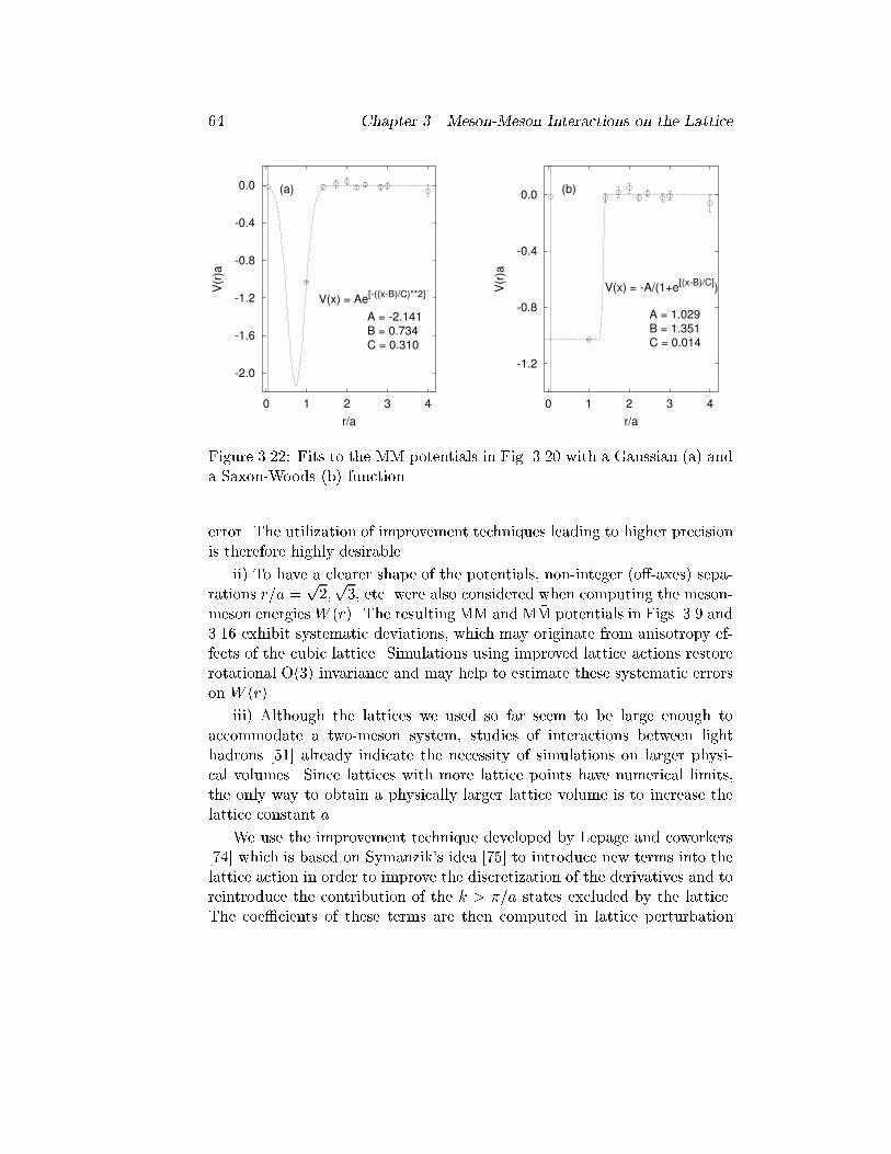
64 Chapter 3. Meson-Meson Interactions on the Lattice

-2.0

-1.6

-1.2

-0.8

-0.4

0.0

0 1 2 3 4

V(r

)a

r/a

V(x) = Ae[-((x-B)/C)**2]

A = -2.141B = 0.734C = 0.310

(a)

-1.2

-0.8

-0.4

0.0

0 1 2 3 4

V(r

)a

r/a

V(x) = -A/(1+e[(x-B)/C]

)

A = 1.029B = 1.351

(b)

C = 0.014

Figure 3.22: Fits to the M �M potentials in Fig. 3.20 with a Gaussian (a) anda Saxon-Woods (b) function.error. The utilization of improvement techniques leading to higher precisionis therefore highly desirable.ii) To have a clearer shape of the potentials, non-integer (o�-axes) sepa-rations r=a = p2;p3; etc. were also considered when computing the meson-meson energiesW (r). The resulting MM and M �M potentials in Figs. 3.9 and3.16 exhibit systematic deviations, which may originate from anisotropy ef-fects of the cubic lattice. Simulations using improved lattice actions restorerotational O(3) invariance and may help to estimate these systematic errorson W (r).iii) Although the lattices we used so far seem to be large enough toaccommodate a two-meson system, studies of interactions between lighthadrons [51] already indicate the necessity of simulations on larger physi-cal volumes. Since lattices with more lattice points have numerical limits,the only way to obtain a physically larger lattice volume is to increase thelattice constant a.We use the improvement technique developed by Lepage and coworkers[74] which is based on Symanzik's idea [75] to introduce new terms into thelattice action in order to improve the discretization of the derivatives and toreintroduce the contribution of the k > �=a states excluded by the lattice.The coe�cients of these terms are then computed in lattice perturbation

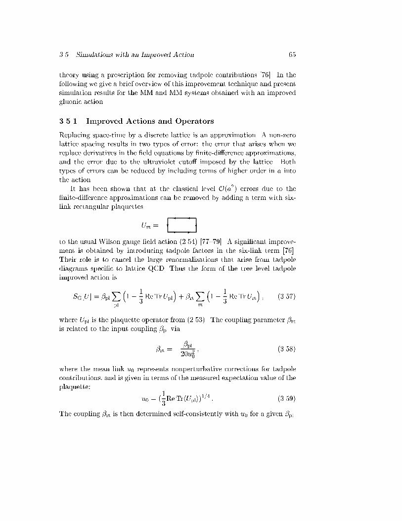
3.5. Simulations with an Improved Action 65theory using a prescription for removing tadpole contributions [76]. In thefollowing we give a brief overview of this improvement technique and presentsimulation results for the MM and M �M systems obtained with an improvedgluonic action.3.5.1 Improved Actions and OperatorsReplacing space-time by a discrete lattice is an approximation. A non-zerolattice spacing results in two types of error: the error that arises when wereplace derivatives in the �eld equations by �nite-di�erence approximations,and the error due to the ultraviolet cuto� imposed by the lattice. Bothtypes of errors can be reduced by including terms of higher order in a intothe action.It has been shown that at the classical level O(a2) errors due to the�nite-di�erence approximations can be removed by adding a term with six-link rectangular plaquettesUrt = ?- - 6��to the usual Wilson gauge �eld action (2.54) [77{79]. A signi�cant improve-ment is obtained by introducing tadpole factors in the six-link term [76].Their role is to cancel the large renormalizations that arise from tadpolediagrams speci�c to lattice QCD. Thus the form of the tree level tadpoleimproved action isSG[U ] = �plXpl �1� 13 ReTrUpl�+ �rtXrt �1� 13 ReTrUrt� ; (3.57)where Upl is the plaquette operator from (2.53). The coupling parameter �rtis related to the input coupling �pl via�rt = � �pl20u20 ; (3.58)where the mean link u0 represents nonperturbative corrections for tadpolecontributions, and is given in terms of the measured expectation value of theplaquette: u0 = (13ReTrhUpli)1=4 : (3.59)The coupling �rt is then determined self-consistently with u0 for a given �pl.

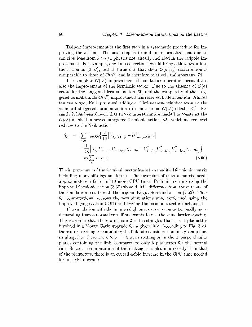
66 Chapter 3. Meson-Meson Interactions on the LatticeTadpole improvement is the �rst step in a systematic procedure for im-proving the action. The next step is to add in renormalizations due tocontributions from k>�=a physics not already included in the tadpole im-provement. For example, one-loop corrections would bring a third term intothe action in (3.57), but it turns out that their O(a2�s) contribution iscomparable to those of O(a4) and is therefore relatively unimportant [74].The complete O(a2) improvement of our lattice operators necessitatesalso the improvement of the fermionic sector. Due to the absence of O(a)errors for the staggered fermion action [80] and the complexity of the stag-gered formalism, its O(a2) improvement has received little attention. Almostten years ago, Naik proposed adding a third-nearest-neighbor term to thestandard staggered fermion action to remove some O(a2) e�ects [81]. Re-cently it has been shown, that two counterterms are needed to construct theO(a2) on-shell improved staggered fermionic action [82], which at tree levelreduces to the Naik actionSF = Xx;� �x� ��xn 916hUx��x+� � U yx��;��x��i� 148hUx�Ux+�;�Ux+2�;��x+3� � U yx��;�U yx�2�;�U yx�3�;��x�3�io+mXx ��x�x : (3.60)The improvement of the fermionic sector leads to a modi�ed fermionic matrixincluding more o�-diagonal terms. The inversion of such a matrix needsapproximately a factor of 10 more CPU time. Preliminary runs using theimproved fermionic action (3.60) showed little di�erence from the outcome ofthe simulation results with the original Kogut-Susskind action (2.52). Thusfor computational reasons the new simulations were performed using theimproved gauge action (3.57) and leaving the fermionic sector unchanged.The simulation with the improved gluonic sector is computationally moredemanding than a normal run, if one wants to use the same lattice spacing.The reason is that there are more 2 � 1 rectangles than 1 � 1 plaquettesinvolved in a Monte Carlo upgrade for a given link. According to Fig. 3.23,there are 6 rectangles containing the link into consideration in a given plane,so altogether there are 6 � 3 = 18 such rectangles in the 3 perpendicularplanes containing the link, compared to only 6 plaquettes for the normalrun. Since the computation of the rectangles is also more costly than thatof the plaquettes, there is an overall 4-fold increase in the CPU time neededfor one MC upgrade.

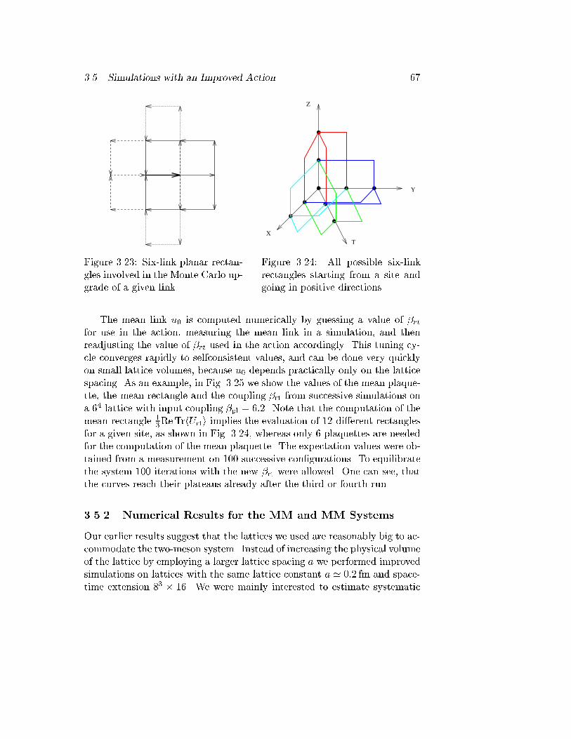
3.5. Simulations with an Improved Action 67

Figure 3.23: Six-link planar rectan-gles involved in the Monte Carlo up-grade of a given link.

Z

T

Y

XFigure 3.24: All possible six-linkrectangles starting from a site andgoing in positive directions.The mean link u0 is computed numerically by guessing a value of �rtfor use in the action, measuring the mean link in a simulation, and thenreadjusting the value of �rt used in the action accordingly. This tuning cy-cle converges rapidly to selfconsistent values, and can be done very quicklyon small lattice volumes, because u0 depends practically only on the latticespacing. As an example, in Fig. 3.25 we show the values of the mean plaque-tte, the mean rectangle and the coupling �rt from successive simulations ona 64 lattice with input coupling �pl = 6:2. Note that the computation of themean rectangle 13ReTrhUrti implies the evaluation of 12 di�erent rectanglesfor a given site, as shown in Fig. 3.24, whereas only 6 plaquettes are neededfor the computation of the mean plaquette. The expectation values were ob-tained from a measurement on 100 successive con�gurations. To equilibratethe system 100 iterations with the new �rt were allowed. One can see, thatthe curves reach their plateaus already after the third or fourth run.3.5.2 Numerical Results for the MM and M �M SystemsOur earlier results suggest that the lattices we used are reasonably big to ac-commodate the two-meson system. Instead of increasing the physical volumeof the lattice by employing a larger lattice spacing a we performed improvedsimulations on lattices with the same lattice constant a ' 0:2 fm and space-time extension 83 � 16. We were mainly interested to estimate systematic

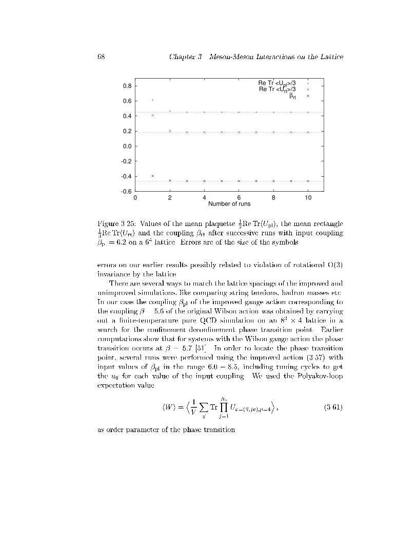
68 Chapter 3. Meson-Meson Interactions on the Lattice

-0.6

-0.4

-0.2

0.0

0.2

0.4

0.6

0.8

0 2 4 6 8 10Number of runs

Re Tr <Upl>/3Re Tr <Urt>/3

βrt

Figure 3.25: Values of the mean plaquette 13ReTrhUpli, the mean rectangle13ReTrhUrti and the coupling �rt after successive runs with input coupling�pl = 6:2 on a 64 lattice. Errors are of the size of the symbols.errors on our earlier results possibly related to violation of rotational O(3)invariance by the lattice.There are several ways to match the lattice spacings of the improved andunimproved simulations, like comparing string tensions, hadron masses etc.In our case the coupling �pl of the improved gauge action corresponding tothe coupling � = 5:6 of the original Wilson action was obtained by carryingout a �nite-temperature pure QCD simulation on an 83 � 4 lattice in asearch for the con�nement-decon�nement phase transition point. Earliercomputations show that for systems with the Wilson gauge action the phasetransition occurs at � = 5:7 [51]. In order to locate the phase transitionpoint, several runs were performed using the improved action (3.57) withinput values of �pl in the range 6:0 � 8:5, including tuning cycles to getthe u0 for each value of the input coupling. We used the Polyakov-loopexpectation value hW i = D 1V X~x Tr NtYj=1Ux=(~x;ja);�=4E ; (3.61)as order parameter of the phase transition.

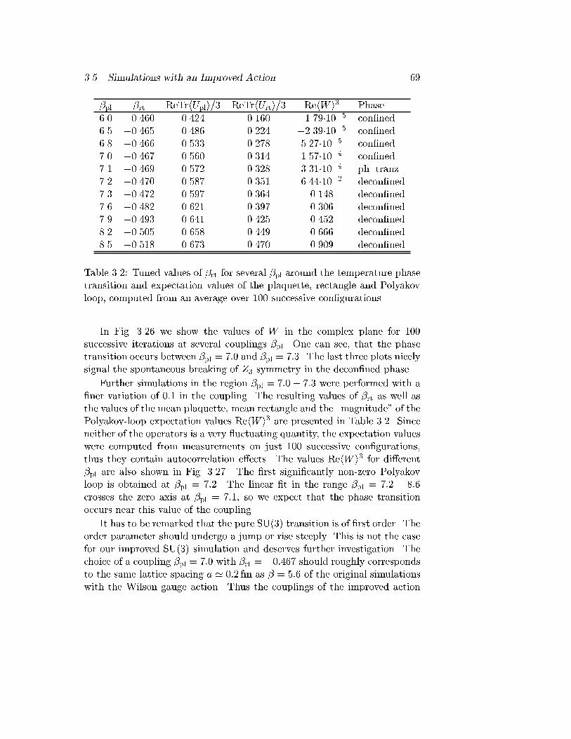
3.5. Simulations with an Improved Action 69�pl �rt ReTrhUpli=3 ReTrhUrti=3 RehW i3 Phase6.0 �0.460 0.424 0.160 �1.79�10�5 con�ned6.5 �0.465 0.486 0.224 �2.39�10�5 con�ned6.8 �0.466 0.533 0.278 5.27�10�5 con�ned7.0 �0.467 0.560 0.314 1.57�10�4 con�ned7.1 �0.469 0.572 0.328 3.31�10�4 ph. tranz.7.2 �0.470 0.587 0.351 6.44�10�2 decon�ned7.3 �0.472 0.597 0.364 0.148 decon�ned7.6 �0.482 0.621 0.397 0.306 decon�ned7.9 �0.493 0.641 0.425 0.452 decon�ned8.2 �0.505 0.658 0.449 0.666 decon�ned8.5 �0.518 0.673 0.470 0.909 decon�nedTable 3.2: Tuned values of �rt for several �pl around the temperature phasetransition and expectation values of the plaquette, rectangle and Polyakovloop, computed from an average over 100 successive con�gurations.In Fig. 3.26 we show the values of W in the complex plane for 100successive iterations at several couplings �pl. One can see, that the phasetransition occurs between �pl = 7:0 and �pl = 7:3. The last three plots nicelysignal the spontaneous breaking of Z3 symmetry in the decon�ned phase.Further simulations in the region �pl = 7:0 � 7:3 were performed with a�ner variation of 0:1 in the coupling. The resulting values of �rt as well asthe values of the mean plaquette, mean rectangle and the \magnitude" of thePolyakov-loop expectation values RehW i3 are presented in Table 3.2. Sinceneither of the operators is a very uctuating quantity, the expectation valueswere computed from measurements on just 100 successive con�gurations,thus they contain autocorrelation e�ects. The values RehW i3 for di�erent�pl are also shown in Fig. 3.27. The �rst signi�cantly non-zero Polyakovloop is obtained at �pl = 7:2. The linear �t in the range �pl = 7:2 � 8:6crosses the zero axis at �pl = 7:1, so we expect that the phase transitionoccurs near this value of the coupling.It has to be remarked that the pure SU(3) transition is of �rst order. Theorder parameter should undergo a jump or rise steeply. This is not the casefor our improved SU(3) simulation and deserves further investigation. Thechoice of a coupling �pl = 7:0 with �rt = �0:467 should roughly correspondsto the same lattice spacing a ' 0:2 fm as � = 5:6 of the original simulationswith the Wilson gauge action. Thus the couplings of the improved action

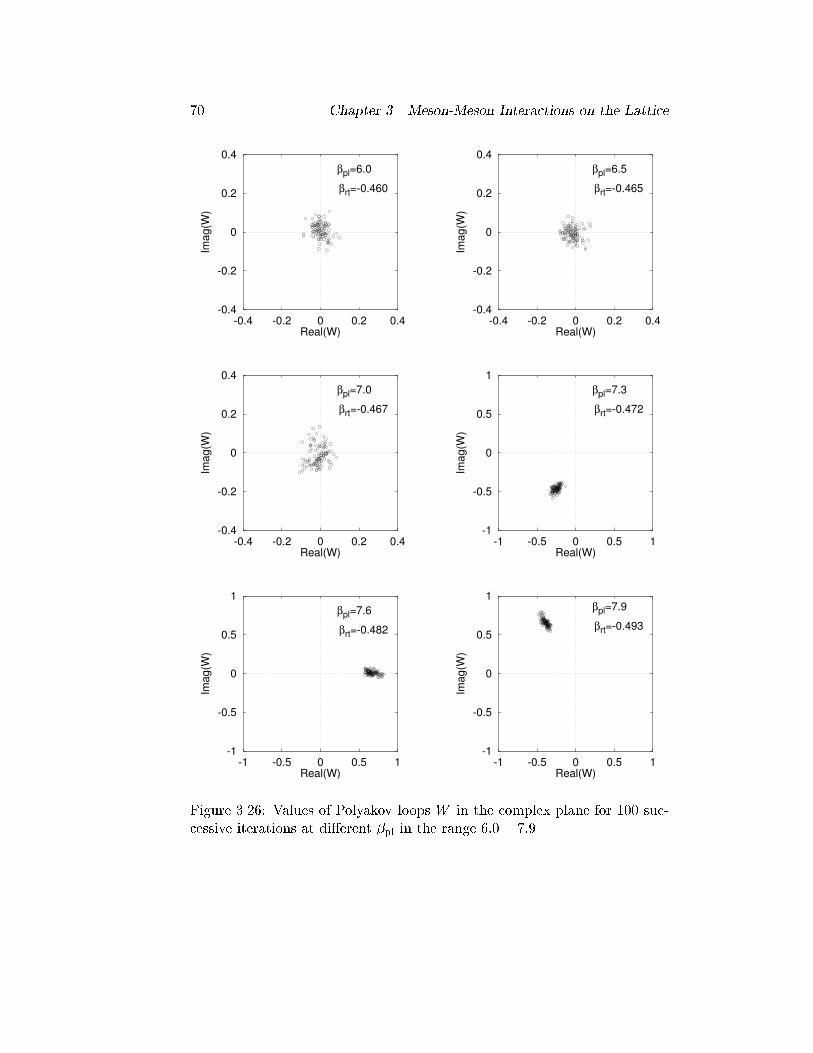
70 Chapter 3. Meson-Meson Interactions on the Lattice-0.4

-0.2

0

0.2

0.4

-0.4 -0.2 0 0.2 0.4

Imag(W

)

Real(W)

βrt=-0.460

βpl=6.0

-0.4

-0.2

0

0.2

0.4

-0.4 -0.2 0 0.2 0.4

Imag(W

)

Real(W)

βrt=-0.465

βpl=6.5

-0.4

-0.2

0

0.2

0.4

-0.4 -0.2 0 0.2 0.4

Imag(W

)

Real(W)

βrt=-0.467

βpl=7.0

-1

-0.5

0

0.5

1

-1 -0.5 0 0.5 1

Imag(W

)

Real(W)

βrt=-0.482

βpl=7.6

-1

-0.5

0

0.5

1

-1 -0.5 0 0.5 1

Imag(W

)

Real(W)

βrt=-0.493

βpl=7.9

-1

-0.5

0

0.5

1

-1 -0.5 0 0.5 1

Imag(W

)

Real(W)

βrt=-0.472

βpl=7.3

Figure 3.26: Values of Polyakov loops W in the complex plane for 100 suc-cessive iterations at di�erent �pl in the range 6:0 � 7:9.

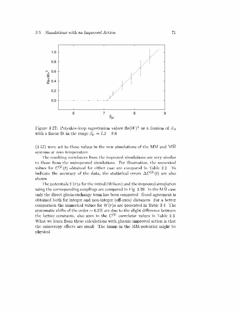
3.5. Simulations with an Improved Action 71

0.0

0.2

0.4

0.6

0.8

1.0

6 7 8 9

Re

<W

>3

βplFigure 3.27: Polyakov-loop expectation values RehW i3 as a funtion of �plwith a linear �t in the range �pl = 7:2� 8:6.(3.57) were set to these values in the new simulations of the MM and M �Msystems at zero temperature.The resulting correlators from the improved simulations are very similarto those from the unimproved simulations. For illustration, the numericalvalues for C(2)(t) obtained for either case are compared in Table 3.3. Toindicate the accuracy of the data, the statistical errors �C(2)(t) are alsoshown.The potentials V (r)a for the initial (Wilson) and the improved simulationusing the corresponding couplings are compared in Fig. 3.28. In the M �M caseonly the direct gluon-exchange term has been computed. Good agreement isobtained both for integer and non-integer (o�-axes) distances. For a bettercomparison the numerical values for W (r)a are presented in Table 3.4. Thesystematic shifts of the order � 0:5% are due to the slight di�erence betweenthe lattice constants, also seen in the C(2) correlator values in Table 3.3.What we learn from these calculations with gluonic improved action is thatthe anisotropy e�ects are small. The hump in the MM-potential might bephysical.

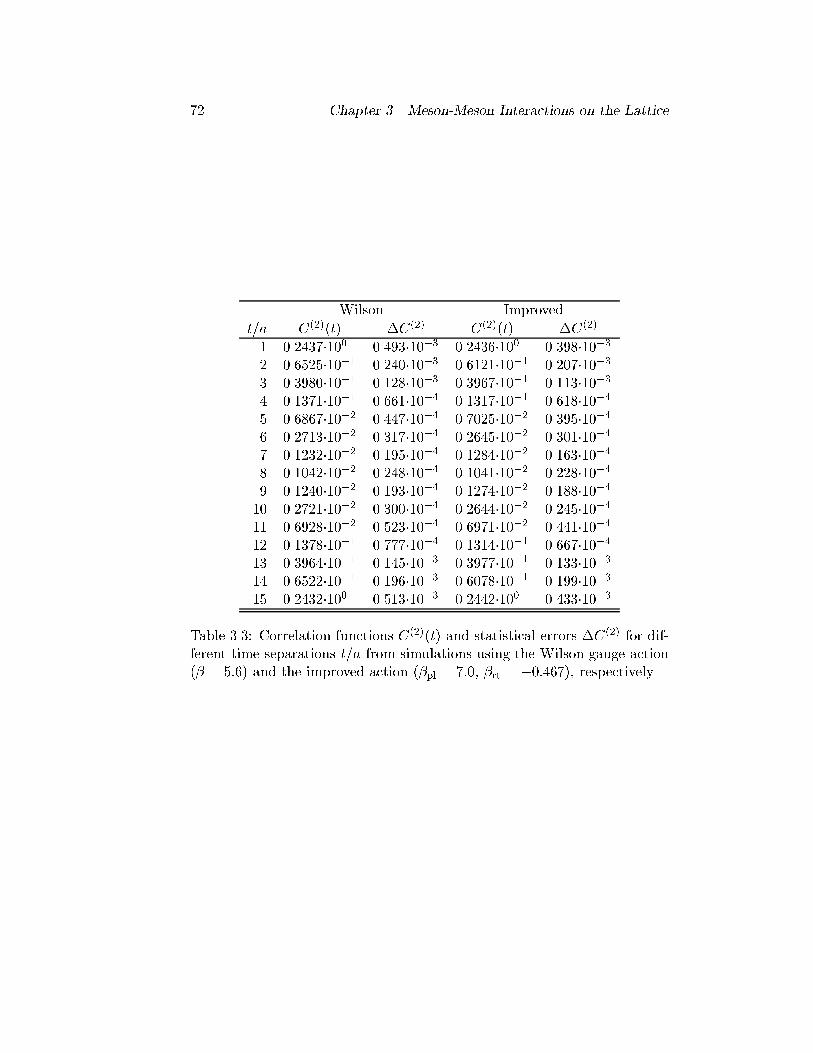
72 Chapter 3. Meson-Meson Interactions on the LatticeWilson Improvedt=a C(2)(t) �C(2) C(2)(t) �C(2)1 0.2437�100 0.493�10�3 0.2436�100 0.398�10�32 0.6525�10�1 0.240�10�3 0.6121�10�1 0.207�10�33 0.3980�10�1 0.128�10�3 0.3967�10�1 0.113�10�34 0.1371�10�1 0.661�10�4 0.1317�10�1 0.618�10�45 0.6867�10�2 0.447�10�4 0.7025�10�2 0.395�10�46 0.2713�10�2 0.317�10�4 0.2645�10�2 0.301�10�47 0.1232�10�2 0.195�10�4 0.1284�10�2 0.163�10�48 0.1042�10�2 0.248�10�4 0.1041�10�2 0.228�10�49 0.1240�10�2 0.193�10�4 0.1274�10�2 0.188�10�410 0.2721�10�2 0.300�10�4 0.2644�10�2 0.245�10�411 0.6928�10�2 0.523�10�4 0.6971�10�2 0.441�10�412 0.1378�10�1 0.777�10�4 0.1314�10�1 0.667�10�413 0.3964�10�1 0.145�10�3 0.3977�10�1 0.133�10�314 0.6522�10�1 0.196�10�3 0.6078�10�1 0.199�10�315 0.2432�100 0.513�10�3 0.2442�100 0.433�10�3Table 3.3: Correlation functions C(2)(t) and statistical errors �C(2) for dif-ferent time separations t=a from simulations using the Wilson gauge action(� = 5:6) and the improved action (�pl = 7:0, �rt = �0:467), respectively.

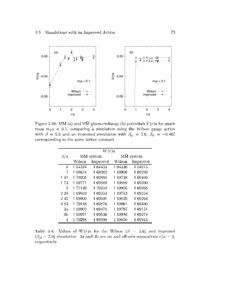
3.5. Simulations with an Improved Action 73

-0.08

-0.04

0.00

0 1 2 3 4

V(r

)a

r/a

mfa = 0.1

(a)

Wilsonimproved

-0.08

-0.04

0.00

0 1 2 3 4V

(r)a

r/a

mfa = 0.1

(b)

Wilsonimproved

Figure 3.28: MM (a) and M �M gluon-exchange (b) potentials V (r)a for quarkmass mfa = 0:1, comparing a simulation using the Wilson gauge actionwith � = 5:6 and an improved simulation with �pl = 7:0, �rt = �0:467corresponding to the same lattice constant.W (r)ar/a MM system M �M systemWilson Improved Wilson Improved0 1.64524 1.64433 1.04336 1.046151 1.68674 1.68382 1.69906 1.692021.41 1.70205 1.69860 1.69738 1.694031.73 1.69771 1.69689 1.69889 1.693002 1.71139 1.70952 1.69955 1.693682.24 1.69803 1.69353 1.69753 1.692542.45 1.69900 1.69601 1.69825 1.692642.83 1.70148 1.69876 1.69961 1.694003a 1.69902 1.69478 1.69797 1.691513b 1.69921 1.69536 1.69946 1.693744 1.70298 1.69908 1.69850 1.69345Table 3.4: Values of W (r)a for the Wilson (� = 5:6) and improved(�pl = 7:0) simulation. 3a and 3b are on and o�-axis separations r=a = 3,respectively.

74 Chapter 3. Meson-Meson Interactions on the Lattice

Chapter 4Summary and ConclusionIn theoretical nuclear physics there is great interest in a fundamental un-derstanding of hadron-hadron interactions. Today, QCD is believed to bethe basic theory of the strong interactions. Since the strong coupling con-stant becomes large in the low energy regime of this theory, phenomena atnuclear distances are problematic to be treated within perturbation theory.Up to now the most successful non-perturbative tool for a calculation ofQCD problems is lattice QCD.This thesis presents pioneering calculations of hadron-hadron potentialsfrom the basic principles of lattice QCD. A practical method to extractan e�ective hadron-hadron potential from hadron Green functions has beendeveloped. This method is a transcription of scattering theory from textbooks to the lattice, and allowed us to take the e�ect of dynamic valencequarks into account. Because of the huge numerical e�ort involved in thetask of calculating hadron four-point correlation functions on the lattice,as a �rst step systems of two pseudoscalar mesons were considered. Thecalculation of baryonic systems has to be postponed to future studies.In one study we investigated the interaction between two heavy-lightmesons. In this approximation the heavy quarks represent static colorsources, which localize the mesons and allow in this way the extraction ofe�ective total energies of the two-meson system from the euclidean time be-havior of the meson four-point correlation function for various inter-mesondistances r. Most of the simulations were performed in quenched lattice QCDwith Kogut-Susskind fermions. The resulting potentials turn out to be shortranged and attractive with a range of about 2 lattice spacings or 0:4 fm, anda depth of approximately 0:04� 0:1 inverse lattice spacing, or 40� 100MeV75

76 Chapter 4. Summary and Conclusionin physical units. Simulations with di�erent light valence-quark masses showthat the interaction is stronger for smaller light-quark masses, but its rangeis always approximately the same. The inclusion of sea quarks did not causedramatic changes in the potentials. The interaction is obviously driven bygluon exchange. Meson exchange out of the dynamic quark sea seems toplay a minor role. A comparison with a simulation on a larger lattice showsthat the e�ect of \mirror" particles is negligible, and that the contributionsfrom excited states do not alter the shape of the potential considerably. Anextrapolation to the chiral limit of the potentials for di�erent light-quarkmasses was performed in order to get closer to physical quark masses. AGaussian form of the potential was obtained from a two-parameter �t tothe resulting data points. This potential was used in a quantum-mechanicalstudy of the behavior of the two-meson system. Despite the attraction forshort distances, neither bound nor resonant meson-meson states were found.In a second study we investigated the interaction between a heavy-lightmeson and its antiparticle. Pure gluon-exchange potentials for the directdiagram as well as potentials in the I = 0 and I = 1 channel were computed.In all cases, the meson-antimeson potentials turn out to be attractive andmuch stronger than the meson-meson potential. The potential in the I = 0channel is of short range|of about 1 lattice spacing or 0:2 fm|and a depthof approximately 0:4 inverse lattice spacing, or 400MeV. We notice a goodqualitative agreement between the simulation results and recent extractionsof K �K potentials from experimental scattering data via inverse scatteringtheory. The potential in the I = 1 channel has a range of about 1:35 latticespacings or 0:27 fm. Its depth could not be determined because of the largeuncertainty of the data point for zero separation. Preliminary quantum-mechanical investigations signal the absence of resonant states also for themeson-antimeson case.We started implementing improved actions into our computer codes inorder to reduce discretization errors, achieve higher precision and make theutilization of larger lattice volumes possible. Results for both the meson-meson and meson-antimeson systems using an O(a2) tree-level and tadpoleimproved gauge action are very close to the unimproved data.There exists a related study of systems of pion-like light-light mesons infour-dimensional lattice QCD following the same method for the calculationof interaction potentials as used in this thesis. It shows a long ranged inter-action between one and �ve lattice spacings, or 0:2 � 1 fm, an intermediateattractive regime with a depth of about 0.05 to 0.2 inverse lattice spacings, or50 to 200 MeV, and a slightly repulsive character below one lattice spacing,

77or 0.2 fm [51, 66].The results obtained in the underlying thesis seem to con�rm phenomenol-ogy. We expect that a re�ned analysis, which besides an improved actionwould include link variable fuzzing and operator smearing in order to enhancethe overlap of the interpolating �elds with the state with minimal energy,will increase the quality of the data and will ultimately lead to quantita-tive results. An independent lattice investigation using Wilson fermions isdesirable, because the assignment of quantum numbers to the interpolatingoperators is straightforward, and consequently physical particles are easilyidenti�ed [83, 84].Studies similar in spirit to the one initiated here may be extended to var-ious other hadron-hadron systems, like kaon-nucleon for example, for whichinversion results exist [65]. Another interesting application would be thequestion of the stability of the doubly strange spin zero H particle as a ��system. Lattice and model studies of this important problem provide con- icting results [85, 86]. The setup of our method makes nuclear physics onthe lattice accessible for realistic investigations.

78 Chapter 4. Summary and Conclusion

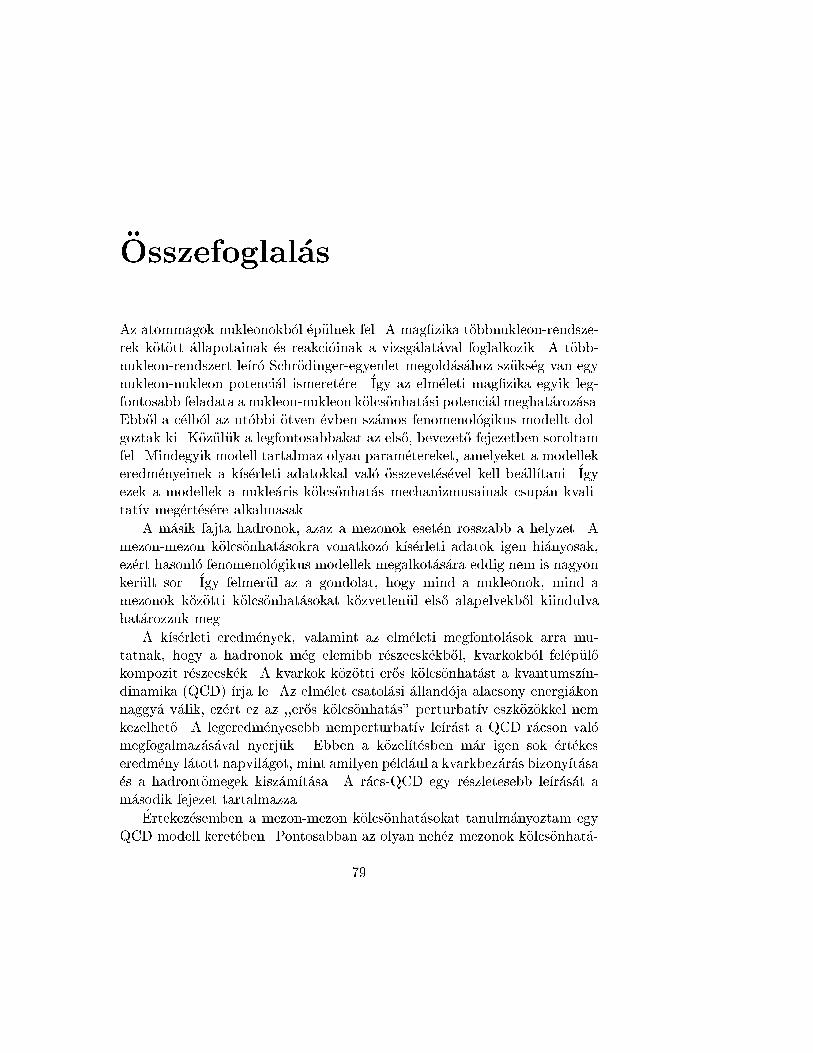
�Osszefoglal�asAz atommagok nukleonokb�ol �ep�ulnek fel. A mag�zika t�obbnukleon-rendsze-rek k�ot�ott �allapotainak �es reakci�oinak a vizsg�alat�aval foglalkozik. A t�obb-nukleon-rendszert le��r�o Schr�odinger-egyenlet megold�as�ahoz sz�uks�eg van egynukleon-nukleon potenci�al ismeret�ere. �Igy az elm�eleti mag�zika egyik leg-fontosabb feladata a nukleon-nukleon k�olcs�onhat�asi potenci�al meghat�aroz�asa.Ebb}ol a c�elb�ol az ut�obbi �otven �evben sz�amos fenomenol�ogikus modellt dol-goztak ki. K�oz�ul�uk a legfontosabbakat az els}o, bevezet}o fejezetben soroltamfel. Mindegyik modell tartalmaz olyan param�etereket, amelyeket a modellekeredm�enyeinek a k��s�erleti adatokkal val�o �osszevet�es�evel kell be�all��tani. �Igyezek a modellek a nukle�aris k�olcs�onhat�as mechanizmusainak csup�an kvali-tat��v meg�ert�es�ere alkalmasak.A m�asik fajta hadronok, azaz a mezonok eset�en rosszabb a helyzet. Amezon-mezon k�olcs�onhat�asokra vonatkoz�o k��s�erleti adatok igen hi�anyosak,ez�ert hasonl�o fenomenol�ogikus modellek megalkot�as�ara eddig nem is nagyonker�ult sor. �Igy felmer�ul az a gondolat, hogy mind a nukleonok, mind amezonok k�oz�otti k�olcs�onhat�asokat k�ozvetlen�ul els}o alapelvekb}ol kiindulvahat�arozzuk meg.A k��s�erleti eredm�enyek, valamint az elm�eleti megfontol�asok arra mu-tatnak, hogy a hadronok m�eg elemibb r�eszecsk�ekb}ol, kvarkokb�ol fel�ep�ul}okompozit r�eszecsk�ek. A kvarkok k�oz�otti er}os k�olcs�onhat�ast a kvantumsz��n-dinamika (QCD) ��rja le. Az elm�elet csatol�asi �alland�oja alacsony energi�akonnaggy�a v�alik, ez�ert ez az ,,er}os k�olcs�onhat�as" perturbat��v eszk�oz�okkel nemkezelhet}o. A legeredm�enyesebb nemperturbat��v le��r�ast a QCD r�acson val�omegfogalmaz�as�aval nyerj�uk. Ebben a k�ozel��t�esben m�ar igen sok �ert�ekeseredm�eny l�atott napvil�agot, mint amilyen p�eld�aul a kvarkbez�ar�as bizony��t�asa�es a hadront�omegek kisz�am��t�asa. A r�acs-QCD egy r�eszletesebb le��r�as�at am�asodik fejezet tartalmazza.�Ertekez�esemben a mezon-mezon k�olcs�onhat�asokat tanulm�anyoztam egyQCD modell keret�eben. Pontosabban az olyan neh�ez mezonok k�olcs�onhat�a-79

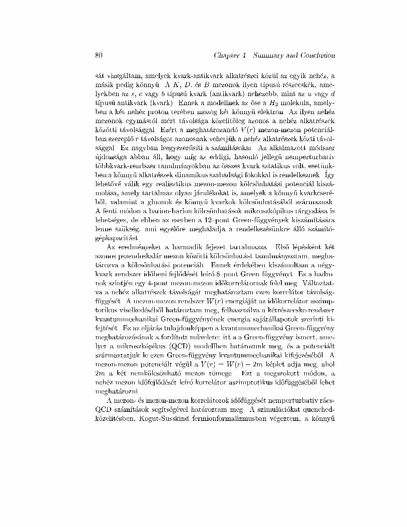
80 Chapter 4. Summary and Conclusions�at vizsg�altam, amelyek kvark-antikvark alkatr�eszei k�oz�ul az egyik neh�ez, am�asik pedig k�onny}u. A K, D, �es B mezonok ilyen t��pus�u r�eszecsk�ek, ame-lyekben az s, c vagy b t��pus�u kvark (antikvark) nehezebb, mint az u vagy dt��pus�u antikvark (kvark). Ennek a modellnek az }ose a H2 molekula, amely-ben a k�et neh�ez proton ter�eben mozog k�et k�onny}u elektron. Az ilyen neh�ezmezonok egym�ast�ol m�ert t�avols�aga k�ozel��t}oleg azonos a neh�ez alkatr�eszekk�oz�otti t�avols�aggal. Ez�ert a meghat�arozand�o V (r) mezon-mezon potenci�al-ban szerepl}o r t�avols�agot azonosnak vehetj�uk a neh�ez alkatr�eszek k�ozti t�avol-s�aggal. Ez nagyban leegyszer}us��ti a sz�am��t�asokat. Az alkalmazott m�odszer�ujdons�aga abban �all, hogy m��g az eddigi, hasonl�o jelleg}u nemperturbat��vt�obbkvark-rendszer tanulm�anyokban az �osszes kvark sztatikus volt, eset�unk-ben a k�onny}u alkatr�eszek dinamikus szabads�agi fokokkal is rendelkeznek. �Igylehet}ov�e v�alik egy realisztikus mezon-mezon k�olcs�onhat�asi potenci�al kisz�a-mol�asa, amely tartalmaz olyan j�arul�ekokat is, amelyek a k�onny}u kvarkcser�e-b}ol, valamint a gluonok �es k�onny}u kvarkok k�olcs�onhat�as�ab�ol sz�armaznak.A fenti m�odon a barion-barion k�olcs�onhat�asok mikroszk�opikus t�argyal�asa islehets�eges, de ebben az esetben a 12{pont Green-f�uggv�enyek kisz�am��t�as�aralenne sz�uks�eg, ami egyel}ore meghaladja a rendelkez�es�unkre �all�o sz�am��t�o-g�epkapacit�ast.Az eredm�enyeket a harmadik fejezet tartalmazza. Els}o l�ep�esk�ent k�etazonos pszeudoskal�ar mezon k�oz�otti k�olcs�onhat�ast tanulm�anyoztam, megha-t�arozva a k�olcs�onhat�asi potenci�alt. Ennek �erdek�eben kisz�amoltam a n�egy-kvark-rendszer id}obeni fejl}od�es�et le��r�o 8{pont Green-f�uggv�enyt. Ez a hadro-nok szintj�en egy 4-pont mezon-mezon id}okorrel�atornak felel meg. V�altoztat-va a neh�ez alkatr�eszek t�avols�ag�at meghat�aroztam ezen korrel�ator t�avols�ag-f�ugg�es�et. A mezon-mezon rendszerW (r) energi�aj�at az id}okorrel�ator aszimp-totikus viselked�es�eb}ol hat�aroztam meg, felhaszn�alva a k�etr�eszecske-rendszerkvantummechanikai Green-f�uggv�eny�enek energia saj�at�allapotok szerinti ki-fejt�es�et. Ez az elj�ar�as tulajdonk�eppen a kvantummechanikai Green-f�uggv�enymeghat�aroz�as�anak a ford��tott m}uvelete: itt a a Green-f�uggv�eny ismert, ame-lyet a mikroszk�opikus (QCD) modellben hat�arozunk meg, �es a potenci�altsz�armaztatjuk le ezen Green-f�uggv�eny kvantummechanikai kifejez�es�eb}ol. Amezon-mezon potenci�alt v�eg�ul a V (r) = W (r) � 2m k�eplet adja meg, ahol2m a k�et nemk�olcs�onhat�o mezon t�omege. Ezt a megszokott m�odon, aneh�ez mezon id}ofejl}od�es�et le��r�o korrel�ator aszimptotikus id}of�ugg�es�eb}ol lehetmeghat�arozni.A mezon- �es mezon-mezon korrel�atorok id}of�ugg�es�et nemperturbat��v r�acs-QCD sz�am��t�asok seg��ts�eg�evel hat�aroztam meg. A szimul�aci�okat quenched-k�ozel��t�esben, Kogut-Susskind fermionformalizmusban v�egeztem, a k�onny}u

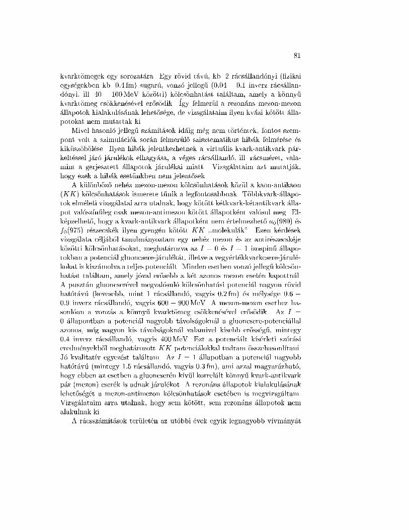
81kvarkt�omegek egy sorozat�ara. Egy r�ovid t�av�u, kb. 2 r�acs�alland�onyi (�zikaiegys�egekben kb. 0:4 fm) sugar�u, vonz�o jelleg}u (0:04 � 0:1 inverz r�acs�allan-d�onyi, ill. 40 � 100MeV k�oz�otti) k�olcs�onhat�ast tal�altam, amely a k�onny}ukvarkt�omeg cs�okken�es�evel er}os�odik. �Igy felmer�ul a rezon�ans mezon-mezon�allapotok kialakul�as�anak lehet}os�ege, de vizsg�alataim ilyen kv�azi k�ot�ott �alla-potokat nem mutattak ki.Mivel hasonl�o jelleg}u sz�am��t�asok id�aig m�eg nem t�ort�entek, fontos szem-pont volt a szimul�aci�ok sor�an felmer�ul}o szisztematikus hib�ak felm�er�ese �eskik�usz�ob�ol�ese. Ilyen hib�ak jelentkezhetnek a virtu�alis kvark-antikvark p�ar-kelt�essel j�ar�o j�arul�ekok elhagy�asa, a v�eges r�acs�alland�o, ill. r�acsm�eret, vala-mint a gerjesztett �allapotok j�arul�ekai miatt. Vizsg�alataim azt mutatj�ak,hogy ezek a hib�ak eset�unkben nem jelent}osek.A k�ul�onb�oz}o neh�ez mezon-mezon k�olcs�onhat�asok k�oz�ul a kaon-antikaon(K �K) k�olcs�onhat�asok ismerete t}unik a legfontosabbnak. T�obbkvark-�allapo-tok elm�eleti vizsg�alatai arra utalnak, hogy k�ot�ott k�etkvark-k�etantikvark �alla-pot val�osz��n}uleg csak mezon-antimezon k�ot�ott �allapotk�ent val�osul meg. El-k�epzelhet}o, hogy a kvark-antikvark �allapotk�ent nem �ertelmezhet}o a0(980) �esf0(975) r�eszecsk�ek ilyen gyeng�en k�ot�ott K �K ,,molekul�ak". Ezen k�erd�esekvizsg�alata c�elj�ab�ol tanulm�anyoztam egy neh�ez mezon �es az antir�eszecsk�ejek�oz�otti k�olcs�onhat�asokat, meghat�arozva az I = 0 �es I = 1 izospin}u �allapo-tokban a potenci�al gluoncsere-j�arul�ek�at, illetve a vegy�ert�ekkvarkcsere-j�arul�e-kokat is kisz�amolva a teljes potenci�alt. Minden esetben vonz�o jelleg}u k�olcs�on-hat�ast tal�altam, amely j�oval er}osebb a k�et azonos mezon eset�en kapottn�al.A puszt�an gluoncser�evel megval�osul�o k�olcs�onhat�asi potenci�al nagyon r�ovidhat�ot�av�u (kevesebb, mint 1 r�acs�alland�o, vagyis 0:2 fm) �es m�elys�ege 0:6 �0:9 inverz r�acs�alland�o, vagyis 600 � 900MeV. A mezon-mezon esethez ha-sonl�oan a vonz�as a k�onny}u kvarkt�omeg cs�okken�es�evel er}os�odik. Az I =0 �allapontban a potenci�al nagyobb t�avols�agokn�al a gluoncsere-potenci�allalazonos, m��g nagyon kis t�avols�agokn�al valamivel kisebb er}oss�eg}u, mintegy0:4 inverz r�acs�alland�o, vagyis 400MeV. Ezt a potenci�alt k��s�erleti sz�or�asieredm�enyekb}ol meghat�arozott K �K potenci�alokkal tudtam �osszehasonl��tani.J�o kvalitat��v egyez�est tal�altam. Az I = 1 �allapotban a potenci�al nagyobbhat�ot�av�u (mintegy 1:5 r�acs�alland�o, vagyis 0:3 fm), ami azzal magyar�azhat�o,hogy ebben az esetben a gluoncser�en k��v�ul korrel�alt k�onny}u kvark-antikvarkp�ar (mezon) cser�ek is adnak j�arul�ekot. A rezon�ans �allapotok kialakul�as�anaklehet}os�eg�et a mezon-antimezon k�olcs�onhat�asok eset�eben is megvizsg�altam.Vizsg�alataim arra utalnak, hogy sem k�ot�ott, sem rezon�ans �allapotok nemalakulnak ki.A r�acssz�am��t�asok ter�ulet�en az ut�obbi �evek egyik legnagyobb v��vm�any�at

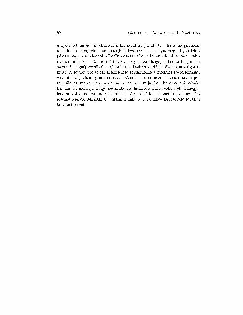
82 Chapter 4. Summary and Conclusiona ,,jav��tott hat�as" m�odszer�enek kifejleszt�ese jelentette. Ezek megjelen�ese�uj, eddig rem�enytelen messzes�egben lev}o t�avlatokat nyit meg. Ilyen lehetp�eld�aul egy, a nukleonok k�olcs�onhat�as�at le��r�o, minden eddigin�el pontosabbr�acsszimul�aci�o is. Ez motiv�alta azt, hogy a sz�am��t�og�epes k�odba be�ep��tsemaz egyik ,,legn�epszer}ubb", a gluonhat�as diszkretiz�aci�oj�at t�ok�eletes��t}o algorit-must. A fejezet utols�o el}otti alfejezete tartalmazza a m�odszer r�ovid le��r�as�at,valamint a jav��tott gluonhat�assal sz�amolt mezon-mezon k�olcs�onhat�asi po-tenci�alokat, melyek j�o egyez�est mutatnak a nem jav��tott hat�assal sz�amoltak-kal. Ez azt mutatja, hogy eset�unkben a diszkretiz�aci�o k�ovetkezt�eben megje-len}o anizotr�opiahib�ak nem jelent}osek. Az utols�o fejezet tartalmazza az el�erteredm�enyek �osszefoglal�oj�at, valamint n�eh�any, a t�em�ahoz kapcsol�od�o tov�abbikutat�asi tervet.

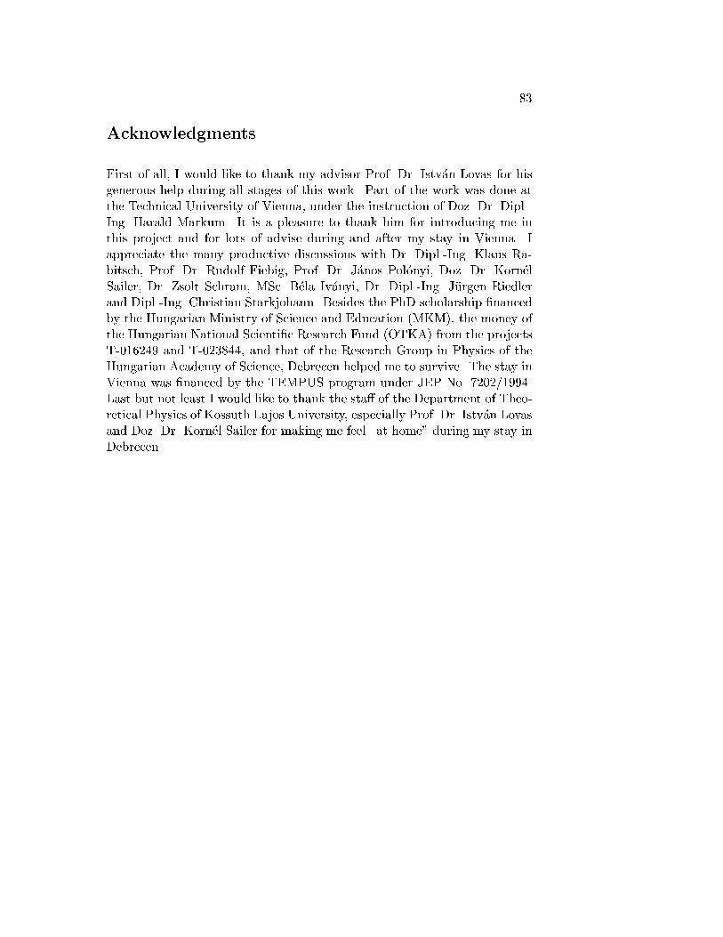
83AcknowledgmentsFirst of all, I would like to thank my advisor Prof. Dr. Istv�an Lovas for hisgenerous help during all stages of this work. Part of the work was done atthe Technical University of Vienna, under the instruction of Doz. Dr. Dipl.-Ing. Harald Markum. It is a pleasure to thank him for introducing me inthis project and for lots of advise during and after my stay in Vienna. Iappreciate the many productive discussions with Dr. Dipl.-Ing. Klaus Ra-bitsch, Prof. Dr. Rudolf Fiebig, Prof. Dr. J�anos Pol�onyi, Doz. Dr. Korn�elSailer, Dr. Zsolt Schram, MSc. B�ela Iv�anyi, Dr. Dipl.-Ing. J�urgen Riedlerand Dipl.-Ing. Christian Starkjohann. Besides the PhD scholarship �nancedby the Hungarian Ministry of Science and Education (MKM), the money ofthe Hungarian National Scienti�c Research Fund (OTKA) from the projectsT-016249 and T-023844, and that of the Research Group in Physics of theHungarian Academy of Science, Debrecen helped me to survive. The stay inVienna was �nanced by the TEMPUS program under JEP No. 7202/1994.Last but not least I would like to thank the sta� of the Department of Theo-retical Physics of Kossuth Lajos University, especially Prof. Dr. Istv�an Lovasand Doz. Dr. Korn�el Sailer for making me feel \at home" during my stay inDebrecen.

84 Chapter 4. Summary and Conclusion

Bibliography[1] L. Eisenbud and E.P. Wigner, Proc. Nat. Acad. Sci. U. S. 27 (1941)281.[2] S. Okubo and R. Marshak, Ann. Phys. 4 (1985) 166.[3] R. V. Reid, Ann. Phys. (N.Y.) 50 (1968) 411.[4] K. Holinde, Phys. Rep. 68 (1981) 121.[5] R. Machleidt, K. Holinde, and Ch. Elster, Phys. Rep. 149 (1987) 1.[6] R. Machleidt, Advances in Nucl. Phys. 19, Plenum (New York, 1989)189.[7] M. Lacombe, B. Loiseau, R. Vinh Mau, J. Cot�e, P. Pir�es, and R. deTourreil, Phys. Rev. C23 (1981) 2405.[8] N. Isgur, in \The New Aspects of Subnuclear Physics", Plenum (NewYork, 1980).[9] C. DeTar, Phys. Rev. D17 (1978) 302.[10] A. Chodos, R. L. Ja�e, K. Johnson, C. B. Thorn, and V. F. Weisskopf,Phys. Rev. D9 (1974) 3471.[11] G. E. Brown and M. Rho, Phys. Lett. B82 (1979) 177.[12] A. W. Thomas, Advances in Nucl. Phys. 13 (1983) 1.[13] G. t'Hooft, unpublished comments at the conference in Marseille (1972).[14] H.D. Politzer, Phys. Rev. Lett. 30 (1973) 1346.[15] K. G. Wilson, Phys. Rev. D10 (1974) 2445.85

86 Bibliography[16] M. Creutz, \Quarks, Gluons and Lattices", Cambridge University Press(Cambridge, 1983).[17] H.J. Rothe, \Lattice Gauge Theories, An Introduction", World Scien-ti�c (Singapore, 1992).[18] I. Montvay and G. M�unster, \Quantum Fields on a Lattice", CambridgeUniversity Press (Cambridge, 1994).[19] D. G. Richards, D. K. Sinclair, and D. Sivers, Phys. Rev. D42 (1990)3191.[20] see A.M. Green and P. Pennanen, Phys. Lett. B426 (1998) 243, andreferences therein.[21] K. Rabitsch, H. Markum, and W. Sakuler, Phys. Lett. B318 (1993) 507.[22] M. Fukugita, Y. Kuramashi, M. Okawa, H. Mino, and A. Ukawa,Phys. Rev. D52 (1995) 3003.[23] R.P. Feynman, Rev. Mod. Phys. 20 (1948) 367.[24] R. P. Feynman and A. R. Hibbs, \Quantum Mechanics and Path Inte-grals", McGraw-Hill (New York 1965).[25] A. Hasenfratz and P. Hasenfratz, Ann. Rev. Nucl. Part. Sci. 35 (1985)559.[26] L. H. Karsten and J. Smit, Nucl. Phys. B183 (1981) 103.[27] H. B. Nielson and M. Ninomiya, Nucl. Phys. B185 (1981) 20.[28] J. Kogut and L. Susskind, Phys. Rev. D11 (1975) 395.[29] L. Susskind, Phys. Rev. D16 (1977) 3031.[30] S. Okubo, Phys. Lett. 5 (1963) 165; G. Zweig, CERN preprint TH 401,412 (1964); J. Iizuka, Prog. Theor. Phys. Suppl. 37 (1966) 21.[31] G. Veneziano, Nuovo Cim. 57A (1968) 190.[32] H. Hamber and G. Parisi, Phys. Rev. Lett. 47 (1981) 1792.[33] D. Weingarten, Phys. Lett. 109B (1982) 57.

Bibliography 87[34] S. Gottlieb, W. Liu, D. Toussaint, R. L. Renken, and R. L. Sugar,Phys. Rev. D35 (1987) 2531.[35] R. T. Scalettar, D. J. Scalapino, and R. L. Sugar, Phys. Rev. B34 (1986)7911.[36] P. Rossi, C.T.H. Davies, and G.P. Lepage, Nucl. Phys. B297 (1988) 287.[37] M.R. Hestenes and E. Stiefel, Nat. Bur. Standards J. Res. 49 (1952)409.[38] J.D. Canosa and H. R. Fiebig, Nucl. Phys. B (Proc. Suppl.) 34 (1994)561.[39] J.D. Canosa, H. R. Fiebig, and H. Markum, Nucl. Phys. B (Proc.Suppl.) 42 (1995) 657.[40] H.R. Fiebig, O. Linsuain, H. Markum, and K. Rabitsch, Nucl. Phys.B (Proc. Suppl.) 47 (1996) 695.[41] H.R. Fiebig, O. Linsuain, H. Markum and K. Rabitsch, Phys. Lett.B386 (1996) 285.[42] J.D. Canosa and H.R. Fiebig, Phys. Rev. D55 (1997) 1487.[43] A. Mih�aly, H.R. Fiebig, H. Markum, and K. Rabitsch, Proceedings of\Hadron Structure '96", Slovac Academy of Science (Bratislava, 1996)172.[44] H.R. Fiebig, H. Markum, A. Mih�aly, K. Rabitsch, W. Sakuler, andC. Starkjohann, Nucl. Phys. B (Proc. Suppl.) 47 (1996) 394.[45] A. Mih�aly, H.R. Fiebig, H. Markum, and K. Rabitsch, Phys. Rev. D55(1997) 3077.[46] H.R. Fiebig, H. Markum, A. Mih�aly, and K. Rabitsch, Nucl. Phys. B(Proc. Suppl.) 53 (1997) 804.[47] H.R. Fiebig, H. Markum, A. Mih�aly and K. Rabitsch, Nucl. Phys. B(Proc. Suppl.) 63A-C (1998) 386.[48] N. Kawamoto and J. Smit, Nucl. Phys. B192 (1981) 100.[49] H. Klugberg-Stern, A. Morel, O. Napoly and B. Petersson, Nucl. Phys.B220 (1983) 447.

88 Bibliography[50] G.W. Kilcup and S.R. Sharpe, Nucl. Phys. B283 (1987) 493.[51] K. Rabitsch, \Hadron-Hadron Potentials from Lattice Quantum Chro-modynamics", Doctoral Thesis, Vienna University of Technology(1997).[52] W. Lucha, F.F. Sch�oberl, and D. Gromes, Phys. Rep. 200 (1991) 127.[53] D. Barkai, K.J.M. Moriarty, and C. Rebbi, Phys. Lett. B156 (1985) 385.[54] W.H. Press, S.A. Teukolsky, W.T. Vetterling, and B.P. Flannery, \Nu-merical Recipes in Fortran", Cambridge University Press, 2nd Edition(Cambridge, 1992) 675.[55] F. Fucito, E. Marinari, G. Parisi, and C. Rebbi, Nucl. Phys. B180[FS2](1981) 369.[56] Particle Data Group: R. M. Barnett et al., Phys. Rev. D54 (1996) 1.[57] J. Sexton, A. Vaccarino, and D. Weingarten, Phys. Rev. Lett. 75 (1995)4563; Nucl. Phys. B (Proc. Suppl.) 53 (1997) 232.[58] G. Bali et al., Phys. Lett. B309 (1993) 378.[59] C. Bernard et al., Nucl. Phys. B (Proc. Suppl.) 53 (1997) 228; C.Bernard et al., Phys. Rev. D56 (1997) 7039.[60] C. Michael and J. Peisa, Nucl. Phys. B (Proc. Suppl.) 63A-C (1998) 55.[61] D.B. Lichtenberg, R. Roncaglia, and E. Predazzi, Proceedings of theInternational Workshop, Diquarks 3, Torino, hep-ph/9611428.[62] T. Vertse, K.F. P�al and Z. Balogh, Comp. Phys. Comm. 27 (1982) 309.[63] J. Weinstein and N. Isgur, Phys. Rev. Lett. 48 (1982) 659.[64] J. Weinstein and N. Isgur, Phys. Rev. D41 (1990) 2236.[65] M. Sander, \Quanteninversion und Hadron-Hadron Wechselwirkun-gen", PhD. Thesis, University of Hamburg, Shaker (Aachen 1997).[66] H.R. Fiebig, H. Markum, A. Mih�aly, K. Rabitsch, M. Sander, and H.V. von Geramb, in preparation.[67] K. K�onigsmann, preprint CERN-PPE/93-182.

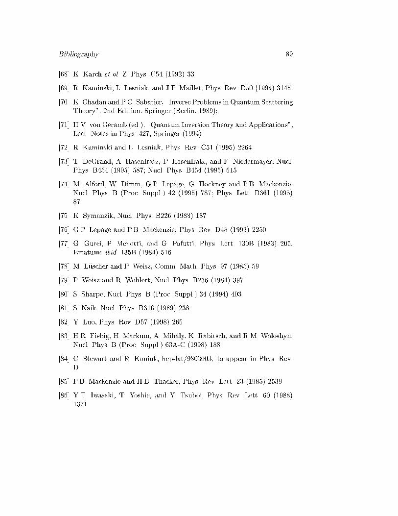
Bibliography 89[68] K. Karch et al. Z. Phys. C54 (1992) 33.[69] R. Kaminski, L. Lesniak, and J.P. Maillet, Phys. Rev. D50 (1994) 3145.[70] K. Chadan and P.C. Sabatier, \Inverse Problems in Quantum ScatteringTheory", 2nd Edition, Springer (Berlin, 1989);[71] H.V. von Geramb (ed.), \Quantum Inversion Theory and Applications",Lect. Notes in Phys. 427, Springer (1994).[72] R. Kaminski and L. Lesniak, Phys. Rev. C51 (1995) 2264.[73] T. DeGrand, A. Hasenfratz, P. Hasenfratz, and F. Niedermayer, Nucl.Phys. B454 (1995) 587; Nucl. Phys. B454 (1995) 615.[74] M. Alford, W. Dimm, G.P. Lepage, G. Hockney and P.B. Mackenzie,Nucl. Phys. B (Proc. Suppl.) 42 (1995) 787; Phys. Lett. B361 (1995)87.[75] K. Symanzik, Nucl. Phys. B226 (1983) 187.[76] G.P. Lepage and P.B. Mackenzie, Phys. Rev. D48 (1993) 2250.[77] G. Gurci, P. Menotti, and G. Pafutti, Phys. Lett. 130B (1983) 205,Erratum: ibid. 135B (1984) 516.[78] M. L�uscher and P. Weisz, Comm. Math. Phys. 97 (1985) 59.[79] P. Weisz and R. Wohlert, Nucl. Phys. B236 (1984) 397.[80] S. Sharpe, Nucl. Phys. B (Proc. Suppl.) 34 (1994) 403.[81] S. Naik, Nucl. Phys. B316 (1989) 238.[82] Y. Luo, Phys. Rev. D57 (1998) 265[83] H.R. Fiebig, H. Markum, A. Mih�aly, K. Rabitsch, and R.M. Woloshyn,Nucl. Phys. B (Proc. Suppl.) 63A-C (1998) 188.[84] C. Stewart and R. Koniuk, hep-lat/9803003, to appear in Phys. Rev.D.[85] P.B. Mackenzie and H.B. Thacker, Phys. Rev. Lett. 23 (1985) 2539.[86] Y.T. Iwasaki, T. Yoshie, and Y. Tsuboi, Phys. Rev. Lett. 60 (1988)1371.

90 Bibliography

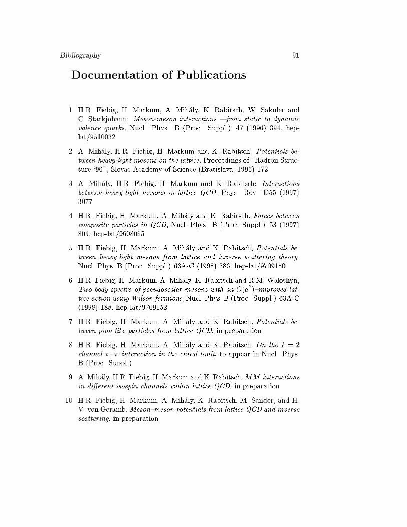
Bibliography 91Documentation of Publications1. H.R. Fiebig, H. Markum, A. Mih�aly, K. Rabitsch, W. Sakuler andC. Starkjohann: Meson-meson interactions { from static to dynamicvalence quarks, Nucl. Phys. B (Proc. Suppl.) 47 (1996) 394, hep-lat/9510032.2. A. Mih�aly, H.R. Fiebig, H. Markum and K. Rabitsch: Potentials be-tween heavy-light mesons on the lattice, Proceedings of \Hadron Struc-ture '96", Slovac Academy of Science (Bratislava, 1996) 172.3. A. Mih�aly, H.R. Fiebig, H. Markum and K. Rabitsch: Interactionsbetween heavy-light mesons in lattice QCD, Phys. Rev. D55 (1997)3077.4. H.R. Fiebig, H. Markum, A. Mih�aly and K. Rabitsch, Forces betweencomposite particles in QCD, Nucl. Phys. B (Proc. Suppl.) 53 (1997)804, hep-lat/9608065.5. H.R. Fiebig, H. Markum, A. Mih�aly and K. Rabitsch, Potentials be-tween heavy-light mesons from lattice and inverse scattering theory,Nucl. Phys. B (Proc. Suppl.) 63A-C (1998) 386, hep-lat/9709150.6. H.R. Fiebig, H. Markum, A. Mih�aly, K. Rabitsch and R.M. Woloshyn,Two-body spectra of pseudoscalar mesons with an O(a2){improved lat-tice action using Wilson fermions, Nucl. Phys. B (Proc. Suppl.) 63A-C(1998) 188, hep-lat/9709152.7. H.R. Fiebig, H. Markum, A. Mih�aly and K. Rabitsch, Potentials be-tween pion-like particles from lattice QCD, in preparation8. H.R. Fiebig, H. Markum, A. Mih�aly and K. Rabitsch, On the I = 2channel �{� interaction in the chiral limit, to appear in Nucl. Phys.B (Proc. Suppl.).9. A. Mih�aly, H.R. Fiebig, H. Markum and K. Rabitsch,M �M interactionsin di�erent isospin channels within lattice QCD, in preparation.10. H.R. Fiebig, H. Markum, A. Mih�aly, K. Rabitsch, M. Sander, and H.V. von Geramb, Meson{meson potentials from lattice QCD and inversescattering, in preparation.

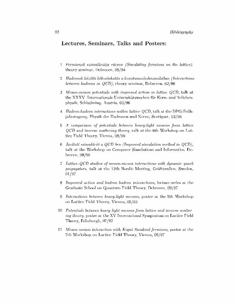
92 BibliographyLectures, Seminars, Talks and Posters:1. Fermionok szimul�aci�oja r�acson (Simulating fermions on the lattice),theory seminar, Debrecen, 09/942. Hadronok k�oz�otti k�olcs�onhat�as a kvantumsz��ndinamik�aban (Interactionsbetween hadrons in QCD), theory seminar, Debrecen, 02/963. Meson-meson potentials with improved action in lattice QCD, talk atthe XXXV. Internationale Universit�atswochen f�ur Kern- und Teilchen-physik, Schladming, Austria, 03/964. Hadron-hadron interactions within lattice QCD, talk at the DPG-Fr�uh-jahrstagung, Physik der Hadronen und Kerne, Stuttgart, 03/965. A comparison of potentials between heavy-light mesons from latticeQCD and inverse scattering theory, talk at the 6th Workshop on Lat-tice Field Theory, Vienna, 09/966. Jav��tott szimul�aci�o a QCD-ben (Improved simulation method in QCD),talk at the Workshop on Computer Simulations and Informatics, De-brecen, 09/967. Lattice-QCD studies of meson-meson interactions with dynamic quarkpropagators, talk at the 12th Nordic Meeting, Gr�aft�avallen, Sweden,01/978. Improved action and hadron-hadron interactions, lecture series at theGraduate School on Quantum Field Theory, Debrecen, 09/979. Interactions between heavy-light mesons, poster at the 5th Workshopon Lattice Field Theory, Vienna, 05/9510. Potentials between heavy-light mesons from lattice and inverse scatter-ing theory, poster at the XV International Symposium on Lattice FieldTheory, Edinburgh, 07/9711. Meson-meson interaction with Kogut-Susskind fermions, poster at the7th Workshop on Lattice Field Theory, Vienna, 09/97