Embed Size (px)
Citation preview
STUDIES OF EARTH DYNAMICS WITH
THE SUPERCONDUCTING GRAVIMETER
Heikki Virtanen
HELSINKI 2006


STUDIES OF EARTH DYNAMICS WITH
THE SUPERCONDUCTING GRAVIMETER
Heikki Virtanen
Academic dissertation in Geophysics
To be presented, with the permission of the Faculty of Science
of the University of Helsinki, for public criticism in Physicum
Auditorium E204, on April 21, 2006, at 12 o’clock noon.
HELSINKI 2006

Also published as No. 133 in the series of
Suomen Geodeettisen laitoksen julkaisuja
Veröffentlichungen des Finnischen Geodätischen Institutes
Publications of the Finnish Geodetic Institute
ISBN-13: 958-951-711-255-0 (nid.)
ISBN-10: 951-711-255-6 (nid.)
ISBN-13: 978-952-10-3057-4 (PDF)
ISBN-10: 952-10-3057-7 (PDF)

“...Concluding on a lighter topic, let me remind the GGP community of what I recall as
probably the most memorable moment of the first campaign. It occurred at the GGP
Workshop in Munsbach Castle, 1999, when Virtanen was describing the effect of snow
cover on the residual gravity at Metsahovi. He showed a figure of gravity increasing by
about 2 microgal over a 4-h period as men shoveled snow from the roof of the SG station,
when a member of the audience asked why there was an interruption in the rise of gravity,
Heikki said this was a 'tea break'...”
D. Crossley, in Journal of Geodynamics 38/3-4 (2004), p. 234.


5
Abstract
I present investigations of Earth dynamics with the superconducting gravimeter GWR
T020 at Metsähovi from 1994 to 2005. As a necessary background, the history and key
technical details of the installation are given. Then a new data acquisition system (DAS)
developed by the author is described. It has proved reliable and accurate. A pre-requisite
for the study of weak phenomena is the removal of the tides from the gravity record and
the careful treatment of spikes, offsets and drifts. I present the data processing methods and
the development of the local tidal model at Metsähovi and show that improvements help in
the modelling of long-term environmental effects.
First, I have used the T020 as a long-period seismometer to study microseismicity and the
Earth’s free oscillation. I present the annual variation, spectral distribution, amplitude and
the sources of microseism at Metsähovi. High levels of microseism appear to be mainly
generated by low-pressure areas (storms) in the Northern Atlantic.
I have analyzed free oscillations excited by three large earthquakes: the spectra, attenuation
and rotational splitting of the modes. An air pressure correction is required to bring down
the noise level. The lowest modes of all different oscillation types are studied, i.e. the
radial mode 0S0 , the “football mode” 0S2, and the toroidal mode 0T2. This last-mentioned
mode is very weak in the vertical as the component is only generated through the Coriolis
coupling. I have also detected the very low level (0.01 nms-1
) incessant excitation of the
Earth’s free oscillation with the T020.
The recovery of global and regional variations in gravity with the superconducting
gravimeter requires the modelling of local gravity effects. The most important of them is
hydrology. The variation in the groundwater level at Metsähovi as measured in a borehole
in the fractured bedrock correlates significantly (0.79) with gravity. The range of the
gravity effect is 70 nms-2
and this phenomenon must be taken into account at an early stage
of data processing. The influence of local precipitation, soil moisture and snow cover are
detectable in the gravity record. A fortuitous experiment powerfully demonstrated the
effect of snow on the laboratory roof, on that occasion -20 nms-2
.
The gravity effect of the variation in atmospheric mass (range about 300 nms-2
) and that of
the non-tidal loading by the Baltic Sea (range about 50 nms-2
) were investigated together,
as sea level and air pressure are correlated. The effects were modelled both using
regression on the local barometer and tide gauge, and with a Green’s function formalism
based a detailed model of the load. In the regression approach, there is a trade-off between
the coefficients. Using Green’s functions it was calculated that a 1 metre uniform layer of
water in the Baltic Sea increases the gravity at Metsähovi by 31 nms-2
and the vertical
deformation is –11 mm. Best results were obtained using the HIRLAM (High Resolution
Limited Area Model) for the atmosphere. Regression on the sea level in Helsinki then
decreases the RMS of gravity residuals by 16%, i.e. explains about 30% of their variance.
The regression coefficient for sea level is 27 nms-2
m-1
, which is 87% of the uniform model.
These studies are associated with temporal height variations using the GPS data of
Metsähovi permanent station. Loading by air pressure and the Baltic Sea explains about
40% of the variance of daily GPS height solution.
6
Acknowledgements
I am grateful to the late Professor Aimo Kiviniemi, my former Department Chief and to
Professor emeritus Juhani Kakkuri, retired Director General, who initiated the operational
work with the superconducting gravimeter at Metsähovi.
The atmosphere at the Finnish Geodetic Institute has been favourable and encouraging for
a research work. I would like to express my appreciation to Professor Risto Kuittinen,
Director General, to Professor Jussi Kääriäinen, the former Chief of the Department of
Gravimetry and to Professor Markku Poutanen, Chief of the Department of Geodesy and
Geodynamics.
Special thanks to my mentor Doc. Jaakko Mäkinen for excellent advisement and for
encouraging a scientific way of thinking for years.
I wish to express my gratitude for the fruitful co-operation with the Finnish Institute of
Marine Research and the Finnish Meteorological Institute.
I wish to thank particularly my colleagues in the Department of Geodesy and
Geodynamics for an assistance of maintenance the instrument and thanks are extended to
the whole friendly staff of the institute.
My warmest thanks finally, got to my wife Marjatta and to my children Riikka, Mikko and
Venla for their patience due to lengthy workdays throughout last years.
Helsinki, March 10, 2006 Heikki Virtanen

7
Contents
List of used abbreviations………………….…………………………………...… 8
List of publications……………………………………………………… ……….. 9
1. Introduction…………………………………………………………...… 10
1.1. Superconducting gravimeter as a research tool…………………………. 10
1.2. Temporal variation in gravity………………………………………...… 10
2. Installation and data processing……………………………………...…. 11
2.1. Site description………………………………………………………….. 11
2.2. Operating history…………………………………………………….…. 13
2.3. Calibration………………………………………………………….…… 13
2.4. Data processing…………………………………………………………. 13
2.5. The new data acquisition system……………………………………….. 15
3. The seismic frequency band…………………………………………….. 18
3.1. Seismic background noise…………………………………………….… 18
3.2. Microseism……………………………………………………………… 19
3.3. Free oscillation of the Earth…………………………………………….. 19
3.4. Incessant excitation of the Earth’s free oscillation………………...…… 21
4. The tidal frequency band…………………………………………...…… 23
4.1. Tidal models at Metsähovi……………………………………...………. 23
4.2. Long period tides……………………………………………………..… 25
5. Atmospheric effects and the Baltic Sea loading……………………..…. 26
5.1. Single admittance for air pressure and modeled Baltic Sea………..…… 26
5.2. Air pressure grid and single tide gauge…………………………….…… 27
5.3. Vertical motion due to loading and GPS………………………….……. 27
5.4. The effects of different tidal models……………………………….…… 27
6. Hydrological effects on gravity………………………………….……… 28
6.1. Instrumentation and available data……………………………….…….. 28
6.2. Results of local studies……………………………………….……….. 29
6.3. Regional and global hydrology…………………………………….…… 30
7. Summary and conclusions……………………………………………… 31
References………………………………………………………………………... 32
Appendices 1,2,3…………………………………………………………………. 37
Publications I, II, III, IV, V and VI…………………………………………...….. 43

8
List of used abbreviations
AP air pressure
CHAMP CHAllenging Minisatellite Payload
CSGI Canadian Superconducting Gravimeter Installation
DAS data acquisition system
DSL Sea level at Degerby tidegauge
ETERNA Eterna program package v. 3.30 (3.40), Wenzel, H-G, 1996)
FGI Finnish Geodetic Institute
FCN Free core nutation
GFZ Geforschung Zentrum in Potsdam.
GGP Global Geodynamics Project
GGP-ISDC GGP Information System and Data Center (GFZ)
(http://ggp.gfz-potsdam.de).
GGP1 Gravity card and filter in GGP project since 1997
GPS Global Positioning System
GRACE Gravity Recovery and Climate Experiment
GW Groundwater level (local at Metsähovi)
GWR Manufacturer of SG:s (San Diego, California, USA)
HIRLAM High Resolution Limited Area Model (air pressure)
HSL Sea level at Helsinki tidegauge
ICET International Center for Earth Tides
LTM Local tidal model
ME Metsähovi station
MS microseims
SG superconducting gravimeter
SNM Seismic Noise Magnitude
TSIP Trimble Standard Interface Protocol
TSOFT Software package for the analysis of time series and Earth tides
T020 SG at Metsähovi
WSFS Watershed Simulation and Forecasting System

9
List of Publications
This thesis consists of 6 published papers and this review. The papers are referred using
roman numerals in brackets. They are:
I. Virtanen, H., 1996. Observations of free oscillations of the Earth by
superconducting gravimeter GWR T020. Acta Geod. Geoph. Mont. Hung. Vol 31,
423-431.
II. Virtanen, H., 1998. On superconducting gravimeter observations above 8 mHz at
the Metsähovi station, Finland. Rep. Finn. Geod. Inst. 98:5.
III. Virtanen H., 2000. On the observed hydrological environmental effects on gravity
at the Metsähovi station, Finland. In B. Ducarme and J. Barthélemy (eds):
Proceedings of the Workshop: High Precision Gravity Measurements with
Application to Geodynamics, and Second GGP Workshop. Munsbach Castle
(Grand Duchy of Luxembourg), March 24th to 26th. Cahiers du Centre Européen
de Géodynamique et de Séismologie 17, 169-175.
IV. Virtanen H., 2001. Hydrological studies at the gravity Station Metsähovi in
Finland. Journal of the Geodetic Society of Japan 47 (1), 328 - 333.
V. Virtanen, H., Mäkinen, J., 2003. The effect of the Baltic Sea level on gravity at
the Metsähovi station, Journal of Geodynamics 35/4-5, 553-565.
VI. Virtanen, H., 2004. Loading effects in Metsähovi from the atmosphere and the
Baltic Sea, Journal of Geodynamics 38/3-5, 407-422.
Paper [I] investigates free oscillations of the Earth, observed after the major earthquake
(Mw 8.2) in Kuril Islands on October 4th, 1994. Paper [II] studies the characteristics of
microseismic and seismic background noise in Metsähovi. Papers [III] and [IV] analyse
the gravity effects of hydrological phenomena, such as variation in groundwater level,
precipitation, soil moisture and snow cover. Papers [V] and [VI] examine the gravity effect
of the variation in atmospheric mass, and of the loading by the Baltic Sea. They utilize
both regression methods based on a single tide gauge/barometer, and calculations with
detailed models for the surface loads. Paper [VI] also associates the loading effects with
temporal height variations using the GPS data of Metsähovi permanent station.
Papers [III, IV, V and VI] have been peer reviewed. Papers [I, II, III, IV and VI] were
written by me alone. Paper [V] was written together with J. Mäkinen. I took the initiative,
processed the gravity data, and made the loading calculations and the graphics. J. Mäkinen
contributed statistical and oceanographic knowledge. The final version was then produced
together.
To provide the necessary background, this review first gives the description of the SG
installation, data acquisition and processing. Then the investigations in the papers [I-VI]
are summarized, updated and complemented where needed. Some relevant new results,
e.g. tidal analyses are given.

10
1. Introduction
1.1. Superconducting gravimeter as a research tool
The superconducting (or cryogenic) gravimeter is based on the levitation of a super-
conducting sphere in a stable magnetic field created by current in superconducting coils
(Prothero and Goodkind, 1968; Warburton and Brinton 1995; Goodkind, 1999).
Depending on frequency, it is capable of detecting gravity1 variations as small as 10
-11ms
-2.
For a single event, the detection threshold is higher, conservatively about 10-9
ms-2
. An SG
can also be used as a long-periodic seismometer (Widmer-Schnidrig, 2003).
Due to its high sensitivity and low drift rate, the SG is eminently suitable for the study
of geodynamical phenomena through their gravity signatures (Hinderer and Crossley,
2000; Jentzsch, et al. 2004). The process is recursive: the gravity record is corrected for
known effects, in order to reduce noise and detect smaller and smaller phenomena.
The superconducting gravimeter GWR T020 (Fig. 1.1) has worked continuously in
Metsähovi, Finland since August 1994 (Virtanen and Kääriäinen 1995; 1997). Metsähovi
is a multi-technique geodetic laboratory including absolute gravity, permanent GPS,
GLONASS, satellite laser ranging, DORIS beacon and geodetic VLBI. They are
influenced by the same environmental effects as the SG. With its high sensitivity, the SG is
an excellent tool for testing and validating the pertinent correction models.
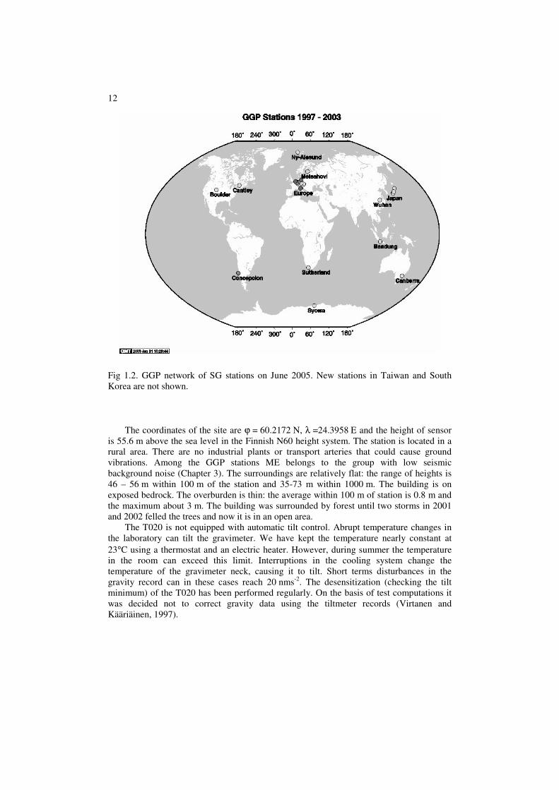
The T020 is a part of the GGP network (Crossley et al., 1999). The GGP worldwide
network (Fig. 1.2) consists of 20 working stations (status June 2005). Station are
concentrated in Europe and Japan. The first phase of the project was 1997-2003,
continuing as phase 2 (2003-2007). The achievements of phase 1 were published in a
special issue of Journal of Geodynamics (Jentzsch et al., 2004). The data of the T020 and
of other participating SGs are available to the scientific community through the GGP-
ISDC (Global Geodynamics Project Information System and Data Center) at GFZ.
One of the original goals of the GGP is the detection of the translational motion of the
solid inner core, or the Slichter triplet, in the sub-seismic band. Its periods due to rotational
splitting constrain the density contrast at the inner core boundary, and even its viscosity
(Smylie et al., 2001). Despite low noise levels in the band from 3 to 6 hours and advanced
methods (e.g. stacking), the detection is still an open challenge to GGP community
(Hinderer and Crossley, 2004)
Although the SGs only provide point measurements, comparisons with the regional gravity
variations observed with the satellites CHAMP and GRACE have proved fruitful (Crossley
and Hinderer, 2002; Crossley et al., 2004; 2005; Neumeyer et al. 2004; 2006). This will be
discussed in Section 6.3.
1.2. Temporal variation in gravity
SG observes the vertical component of gravity, and the vertical acceleration of Earth
surface. The temporal variation in gravity consists of numerous phenomena with different
periods and amplitudes. Earth tides have the strongest effect, in ME about 2250×10-9
ms-2
peak to peak (p-p). The next largest is the variable gravity effect of the atmosphere. The
range of atmospheric pressure at ME is about 100 hPa, corresponding 300×10-9
ms-2
in
gravity. The pole tide in ME is 80×10-9
ms-2
(p-p). Hydrological phenomena such as
1 In this review SI units are used. However, in some of the Papers occasionally the cgs-unit
“gal” was used (1 gal=10-2
ms-2
, 1 µgal=10-8
ms-2
, 1 ngal=10-11
ms-2
)

11
variation in soil moisture content, groundwater level and snow cover have an influence up
to 80×10-9
ms-2
. The loading effect of the Baltic Sea varies about 40×10-9
ms-2
(p-p). An
extensive review of environmental effects of gravity is given by Van Dam and Wahr
(1998).
The ground acceleration due to strong earthquakes exceeds all magnitudes above. The
effect of a strong microseism (MS) can be about 1000×10-9
ms-2
. Weakest observable
periodical phenomena, such as free oscillations of the Earth are 0.01×10⁻⁹
ms-2
in amplitude
(Chapter 3).
Fig. 1.1. Superconducting gravimeter T020 in gravity laboratory at Metsähovi.
2. Installation and data processing
2.1. Site description
The SG T020 was installed in a specially designed gravity laboratory at Metsähovi in
August 1994. The building and the gravimeter pier stand on a knoll of Precambrian
granite. The T020 is equipped with a 200 litre Dewar for liquid helium. Technical details
are given by Warburton and Brinton (1995) and in the GWR operating manual (GWR,
1989). A general description of the T020 system, gravity laboratory and DAS (until July
2003) is given by Virtanen and Kääriäinen (1995;1997).
12
Fig 1.2. GGP network of SG stations on June 2005. New stations in Taiwan and South
Korea are not shown.
The coordinates of the site are ϕ = 60.2172 N, λ =24.3958 E and the height of sensor
is 55.6 m above the sea level in the Finnish N60 height system. The station is located in a
rural area. There are no industrial plants or transport arteries that could cause ground
vibrations. Among the GGP stations ME belongs to the group with low seismic
background noise (Chapter 3). The surroundings are relatively flat: the range of heights is
46 – 56 m within 100 m of the station and 35-73 m within 1000 m. The building is on
exposed bedrock. The overburden is thin: the average within 100 m of station is 0.8 m and
the maximum about 3 m. The building was surrounded by forest until two storms in 2001
and 2002 felled the trees and now it is in an open area.
The T020 is not equipped with automatic tilt control. Abrupt temperature changes in
the laboratory can tilt the gravimeter. We have kept the temperature nearly constant at
23°C using a thermostat and an electric heater. However, during summer the temperature
in the room can exceed this limit. Interruptions in the cooling system change the
temperature of the gravimeter neck, causing it to tilt. Short terms disturbances in the
gravity record can in these cases reach 20 nms-2
. The desensitization (checking the tilt
minimum) of the T020 has been performed regularly. On the basis of test computations it
was decided not to correct gravity data using the tiltmeter records (Virtanen and
Kääriäinen, 1997).
13
2.2. Operating history
The gravimeter itself has been working continuously since installation in August
1994, but malfunctions of the DAS have caused about ten interruptions in the registration.
Typically gaps were a day or two. The second longest gap was two weeks. The longest gap
was caused by a thunderbolt, which destroyed the GPS receiver of the installation on July
5, 2003. It was necessary to develop a new DAS (Section 2.5) before the registration could
be restarted in November 2003. This data gaps lasted 4 months (Fig. 2.1). Disturbances in
the cooling system have caused some rejection of data in analysing stage (Section 2.4).
In September 1997 the original gravity card was replaced by a new one called GGP1,
following the recommendation of the GGP project (GGP 2006). The main difference
between the cards is the corner frequency in low pass filtering, which is 40 s for the
original card and 16.3 s for the GGP1, which make better possibility to study microseism
[II]. During repair of the GGP1, the old card was again used from March 16, 1999 to
January 3, 2001.
2.3. Calibration
The T020 was calibrated using simultaneous observations with the absolute
gravimeter JILAg-5 in 1995 (Mäkinen et al., 1995; Hinderer et al., 1998). We have
adopted the value 1107 ±3 nms-2
V-1
(one sigma) Thereafter calibration has been checked
occasionally. To obtain a large tidal amplitude, the calibrations were carried out near new
or full moon. Typically, 2400 drops in the absolute gravimeter per day were carried out,
the whole calibration lasting 3-5 days. The latest calibration was made with the absolute
gravimeter FG5-221 in June 2005. The later results were compatible with the original
value within the error limits.
Some comparisons with ocean loading models seem to indicate that the value above is
too high by 0.3 % (i.e. by its standard error). This will be discussed in Section 4.1. A
unified recomputation of all calibration observations accumulated over the years is in
progress. The results presented in papers [I-VI] do not in practice depend on the calibration
factor.
Transfer functions were measured and calculated for the original and for the GGP1
gravity card in September 1997 using the method described by Van Camp et al. (2000). In
the tidal band the lag was 16.6 s and 9.5 s for the original and for the GGP1 card,
respectively (0.0690 and 0.0395 deg/cpd).
In addition to gravity, special attention has been paid to the accuracy of the barometers
(Virtanen, 2003).
2.4. Data processing
For uniformity, all gravity data, originally processed in shorter batches were
reprocessed several times from 1996 to 2005. The current data processing methods are
described in detail in papers [V and VI] and by Virtanen and Mäkinen (2003). The
description will be not repeated here. The data set of paper [VI] ends August 31, 2002. The
same set is used in Chapters 4 and 5. For the paper by Neumayer et al. (2006) and for
Chapter 6 the data set was extended to July 4, 2003. Some stages of data processing are
presented in Figures 2.1, 2.2 and 2.3. Fig 2.1 shows the raw T020 record without any
corrections, only the calibration factor has been applied. In Fig. 2.2 tides, pole tide and air
pressure corrections have been subtracted. Steps and spikes are well visible and the figure
demonstrates the importance of and the difficulties in eliminating drift and offsets,
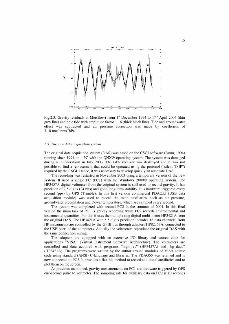
especially for long-term studies. Fig. 2.3 shows the final gravity residual after spikes,
offsets, traces of big earthquakes etc. were removed, the groundwater effect corrected for,

14
and drift eliminated in three separated blocks (Section 4.3). The pole tide has been restored
to the graph to demonstrate the successful preparation of data. The TSOFT 2.0.15 program
package (Van Camp and Vauterin, 2005) was used in the correction processing and
analyses.
The apparent drift rate for the last block of data starting September 1, 2000 was
+31 nms-2
(yr)-1
. The secular gravity change at the site is about -10 nms-2
(yr)-1
according to
the co-located absolute gravimeter record (JILAg-5) and is thought to be due to postglacial
rebound. The net drift of the T020 is thus about 40 nms-2
(yr)-1
.
Fig. 2.1. Gravity data by obtained with T020 at Metsähovi from 12th
August 1994 to 1st
November 2004.
Fig. 2.2. Gravity residuals by T020 shown at Metsähovi 12
th August 1994 – 1
st November
2004. Tide, pole tide was subtracted and air pressure correction was made by coefficient of
3.10 nms-2
hPa-1
.
15
Fig.2.3. Gravity residuals at Metsähovi from 1st December 1994 to 17
th April 2004 (thin
grey line) and pole tide with amplitude factor 1.16 (thick black line). Tide and groundwater
effect was subtracted and air pressure correction was made by coefficient of
3.10 nms-2
nms-2
hPa-1
.
2.5. The new data acquisition system
The original data acquisition system (DAS) was based on the CSGI software (Dunn, 1994)
running since 1994 on a PC with the QNX operating system. The system was damaged
during a thunderstorm in July 2003. The GPS receiver was destroyed and it was not
possible to find a replacement that could be operated using the protocol (“silent TSIP”)
required by the CSGI. Hence, it was necessary to develop quickly an adequate DAS.
The recording was restarted in November 2003 using a temporary version of the new
system. It used a single PC (PC1) with the Windows 2000 operating system. The
HP3457A digital voltmeter from the original system is still used to record gravity. It has
precision of 7.5 digits (24 bits) and good long-term stability. It is hardware triggered every
second (pps) by GPS (Trimble). In this first version commercial PDAQ55 (USB data
acquisition module) was used to record the main auxiliaries, such as air pressure,
groundwater precipitation and Dewar temperature, which are sampled every second.
The system was completed with second PC2 in the summer of 2004. In this final
version the main task of PC1 is gravity recording while PC2 records environmental and
instrumental quantities. For this it uses the multiplexing digital multi-meter HP3421A from
the original DAS. The HP3421A with 5.5 digits precision includes 18 data channels. Both
HP instruments are controlled by the GPIB bus through adapters HP82357A, connected to
the USB ports of the computers. Actually the voltmeters reproduce the original DAS with
the same connection wiring.
The adapters are equipped with an extensive I/O library and source code for
applications ”VISA” (Virtual Instrument Software Architecture). The voltmeters are
controlled and data acquired with programs “high_res” (HP3457A) and “hp_dacu”
(HP3421A). The programs were written by the author around modules of VISA source
code using standard (ANSI) C-language and libraries. The PDAQ55 was retained and is
now connected to PC2. It provides a flexible method to record additional auxiliaries and to
plot them on the screen.
As previous mentioned, gravity measurements on PC1 are hardware triggered by GPS
one-second pulse to voltmeter. The sampling rate for auxiliary data on PC2 is 10 seconds

16
and it is software triggered by PC clock. Both computers keep correct time via an Internet
connection to NIST time servers (e.g. time-b.nist.gov) every 10 minutes. In addition, PC1
is equipped with a DCF radio clock which updates the PC clock every minute. The
accuracy of the PC’s timekeeping is typically 10 ms for PC1 and 20 ms for PC2. All
recorded samples include time and date stamps by PC’s clock.
The most important files such as gravity and air pressure are stored in ASCII format and
the files are identified as “yydoy.xxx” (year and day of year). Both PC1 and PC2 are
connected to the Internet and to the intranet of FGI. Gravity and pressure files can be
downloaded at any time, even while they are still being written. The hard disk space is
sufficient for several years of recording.
The computers are similar standard PC devices. All connections are made using USB
and standard serial ports, no special pc-boards are required. All important software are
installed in both computers. Thus an adequate DAS can quickly be built on a single
computer using only part of the full DAS. This reduces the risk of long data gaps in the
case of computer or other device failure.
Another basic principle in the system design is the remote control. Authorized remote
computers can control systems via VNC (Virtual Network Computing). The computers are
fully remote controlled including boots.
The screens of both computers are shown in Figs. 2.4 and 2.5. The letters in brackets
refer to these Figures. Screen dumps of both computers are sent every 5 minutes to the ftp
server of the FGI. Screen outlooks are seen everywhere later on. We have included some
useful features on the screens. PC1 plot [A] gives the spectrum of 1 second gravity data
from 10 mHz to 500 mHz, updated every ten second. This window gives at a glance
information for MS, surface waves after earthquakes and the general quality of data.
The screen of PC2 [B] shows the gravity output after MODE and TIDE filters and is
updated every minute. The MODE filter is a bandpass filter, periods about 1 min-60 min
(GWR, 1989). This signal is amplified by 20. The TIDE filter is a lowpass filter with cut-
off at 50 seconds. Both outputs are visible in the window, which show the last 48 hours.
The TIDE curve shows output of gravimeter in tidal band and the MODE curve reveals
disturbances, e.g. earthquakes. The plotter programs use the IDL Virtual Machine utility.
Other windows show selectable outputs of the PDAQ55 data acquisition unit [A], E] and
[F]. This device includes a pulse counter, which is connected to the rain gauge [E]. The
device has free channels and if necessary, further expandability. PC2 reads altogether 18
channels [B] including environmental and instrumental temperatures, air pressure and
groundwater, TIDE and MODE signals.
The PC1 has a ftp server and PC2 has the controlling programs for the UPS. The full DAS
consists of many independent pieces, and restarting the entire system is a somewhat
laborious task. On the other hand updating and modification of system parts is more
simpler and an interruption of the whole system is not necessary. The DAS as a whole has
proved to be reliable and flexible. Most importantly, the accuracy of the data and of the
timing are good enough for SG. Due to the importance of air pressure registration, we aim to record more than one
barometer at all time. The sensors outside the laboratory are typically related to
environmental phenomena, such as groundwater level and precipitation (Chapter 6).
On the screen of PC2 one can see the effects of the great earthquake in Sumatra
26.12.2004 UT 00:58 (M9.0). The window [A] shows an exceptionally strong horizontal
acceleration due to the surface waves recorded with the tiltmeters of the SG.

17
Fig 2.4. The screen of the computer PC1. [A] MS MONITOR, (IDL VM), 10s updating,
One hour spectrum for one second data of window [B]. [B] Output of ”High_res” (C-
language) program, 1-second, 7.5 digits high-res resolution gravity data taken with
HP3457A voltmeter triggered by GPS (pps). [C] Output window internet timing, auto-
matically updated every 10 minutes. [D] Control window for computer system. [E] The
program ”TSIPMON32” is needed to start the GPS pps operation. [F] Output of the digital
barometer (Vaisala) PTB220, one second samples. [G] DFC radio clock, PC-time to
atomic time every minute.
Fig 2.5. The screen of the computer PC2. [A] Chart display of PDAQ55 (one second
samples). Speed and channels are selectable. In this case air pressure, tilts of SG (x and y)
are shown, 24 hours are visible. [B] MODE/TIDE PLOTTER (IDL VM), 1-min
updating, data sampled every 10 seconds, last 48-hours are visible with fixed and running
time axes. [C] Output of ”Hp_dacu” (C-language) program, 18 channels are sampled every
10 seconds, accuracy is 5.5 digits. [D] Internet timing output window, automatically
updated every 10 minutes. [F] Main control window of the PDAQ55 data acquisition
module. [E] Digital output of PDAQ55, in this case air pressure and precipitation are
shown. Air pressure is the analog output of the digital barometer PTB220.

18
3. The seismic frequency band
3.1. Seismic background noise
A special concept “Seismic Noise Magnitude” (SNM) has been developed to give an
unambiguous measure of background noise level at any gravity stations (Banka and
Crossley, 1999). It is based on the Power Spectral Density (PSD) calculated from the mean
FFT in the period range 200-600 s. The 5 quiet days of gravity data has been used for
SNM (GGP, 2006). It is defined as:
5.2)log(10 += PSDmeanSNM
For ME the SNM factor is 0.88. It varies from 0.20 (Moxa in Germany, SG CD034) to
2.20 (Brasimore in Italy, SG T015). Later comparisons of the seismic noise levels at
various GGP stations were made by Rosat et al., (2002) and Rosat et al., (2004). The
investigations covered the spectrum between 200 s and 24 h (Rosat et al. 2004). Among 20
SG stations, ME has the 8th
lowest noise magnitude and it belongs to group of low noise
stations. Thus, ME is a very suitable station for studies in the seismic frequency band.
Fig 3.1 presents the PSD of the spectrum from 0.01 mHz to 1000 mHz for three days. The
densities are determined in a similar way as in Banka (1997). This figure updates older
background noise presentations (Fig 14 in [II]). The upper graph shows the spectrum
during quiet days and using the original gravity card (Section 2.2). The MS-band (from
66 mHz to 500 mHz) is strongly attenuated by the low pass filter. The data for next two
spectra were taken with the GGP1 gravity card. The middle graph gives the spectrum
during strong MS, periods for peaks are about 12 seconds and 6 seconds. The bottom
graph represents the spectrum on a quiet day. The thick line indicates the level of New
Low Noise Model, often referred as NLMN (Peterson, 1993).
Fig. 3.1. The Power Spectral Densities from 0.01 mHz to 1000 mHz for one day. Top: Old
gravity card and low MS level (June 14, 1997), Middle: New gravity card and high MS
(January 29, 2003), Bottom: New gravity card (GGP1) and low MS level (30 April 2003).
19
3.2. Microseism
The paper [II] analyses of ME data at periods shorter than 2 minutes (over 8 mHz).
This limit was chosen, because for most applications we use the data filtered to 1 minute.
The paper presents information on the nature of microseism (MS) at Metsähovi. Annual
variations, spectral distributions, amplitudes and sources are given.
There is a clear correlation between the occurrence of low atmospheric pressure (storm) in
the Northern Atlantic Ocean and MS. The usual shape of the spectrum shows two peaks
near 12 and 6 second periods. However, the location of the peaks varies with the source.
Typical examples are the Norwegian coast and the middle Atlantic Ocean. In addition,
distant medium size earthquakes are treated as seismic noise. The amplitude of ground
motion can exceed 0.003 mm during a strong MS. In paper [II] moving window spectrum
for frequencies up to 300 mHz was presented from 10 August 1994 to 28 October 1998.
The effect of changed gravity card (filter cut-off changed) is clearly seen from 5
September 1997. As to the seasonal variation, the period from April to September has
rather low MS and the strongest MS storm occurred often between January and March.
In SG studies outside the seismic band, the MS is generally not a source of uncertainty,
due to the filtering. However other gravity observations (absolute and relative) suffer from
MS and may benefit from insights gained with the SG.
3.3. Free oscillation of the Earth
The paper [I] presents observations of the free oscillation of the Earth after the great
earthquake in Kuril Islands on 4th
October 1994. The spectra were calculated using two
methods: Lomb-Scargle periodogram and FFT. We had 1-minute gravity data, corrected
for air pressure and then used a high pass filter (one hour cutoff). We were able to extract
clearly the lowest spheroidal mode 0S2 (0.30945 mHz, or 54 minutes). Zürn et al. (2000)
noticed this rare observation and the success of air pressure correction in seismic band. In
addition, I presented the attenuation and duration of other spheroidal modes. We were able
to detect radial mode 0S0 (0.81439 mHz or 20 minutes) above level of one nanogal
(10-11
ms-2
) over six weeks. Others modes disappeared during two days. In addition,
graphics of the two dimensional summary was presented from August 1994 to August
1996. [I, p. 430]. We can say that the excitation 0S0 mode has been observed at the one
ngal level at least 25% of total recording time.
Another significant great earthquake (magnitude 8.4) occurred in Peru on June 23,
2001. This quake excited the “football mode” 0S2 with quite high SNR (Widmer-
Schnidrig, 2003). The lowest modes of this quake with T020 are shown in the spectrum of
72-hours in Fig. 3.2. The gravest toroidal mode 0T2 (0.37730 mHz, or 44 minutes) is
clearly discernible. This mode is very seldom detected with vertical instruments as it
influences then through Coriolis coupling only. Individual singlets of the 0S2 mode are
presented in Fig. 3.3 (0.30480, 0.30949 and 0.31400 mHz). In the spectrum of shorter time
series this rotational splitting complicates observing this mode. The longer time series
reveals individual singlets of 0S2. On the other hand the mode 0T2 disappears. In addition,
the splitting of the mode 0S3 (0.46855 mHz) is visible.

20
Fig. 3.2. Free oscillation of the Earth. Peru earthquake 23.06.2001 UT 20:45 (Mw 8.4).
The length of spectrum is 72 hours, since 24.6.2001 UT 9:00. The gravity 1-min data is
hanning windowed, air pressure corrected (-3.10 nms-2
hpa-1
) and high pass filtered
(1 hour). The 1 ngal (10-11
ms-2
) level is shown as dotted line.
Fig. 3.3. Free oscillation of the Earth. Peru earthquake 23.06.2001 UT 20:45 (Mw 8.4).
Splittings of the lowest spheroidal mode 0S2 and the mode 0S3 are visible. The length of
the spectrum is 200 hours, since 23.06.2001 UT 20:45. The gravity 1-min data is hanning
windowed, air pressure corrected (-3.10 nms-2
hpa-1
) and high pass filtered (1 hour). The
1 ngal (10-11
ms-2
) level is shown as dotted line.
21
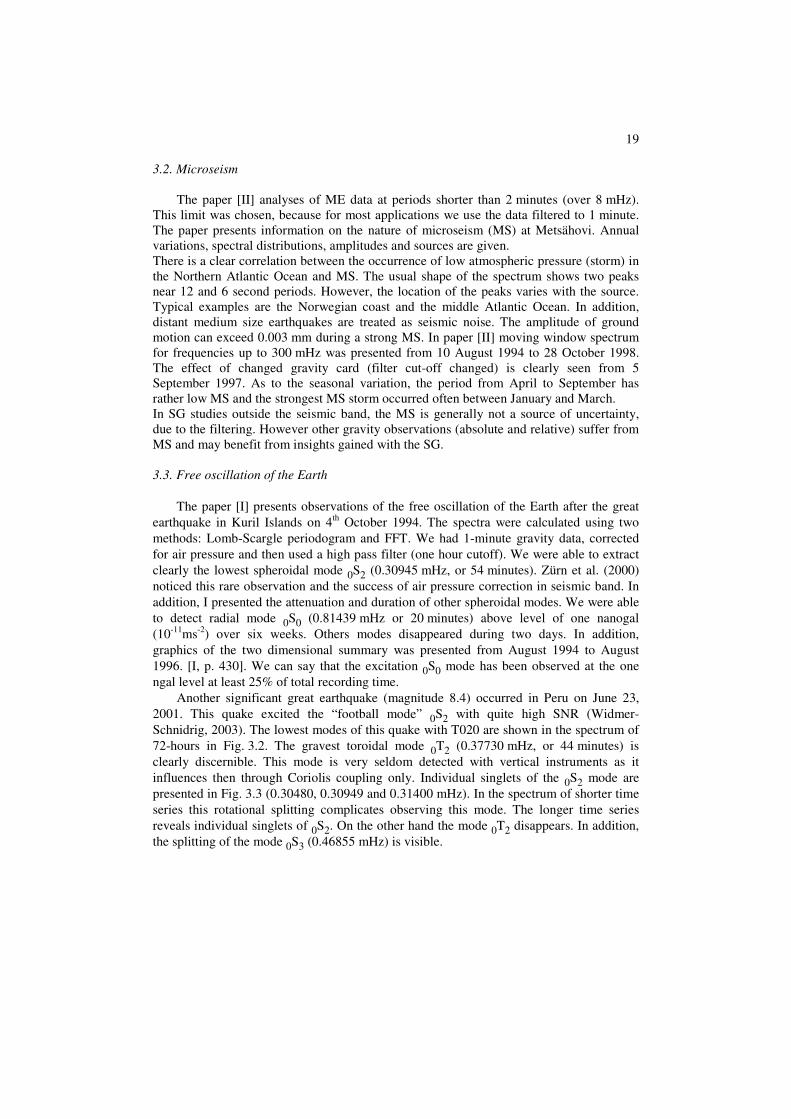
Fig. 3.4. Free oscillation of the Earth. Sumatra earthquake 28.12.2004 UT 00:58 (Mw 9.0).
The length of spectrum is 72 hours, since 26.12.2004 UT 13:00. The gravity 1-min data is
hanning windowed, air pressure corrected (-3.10 nms-2
hpa-1
) and high pass filtered
(1 hour). The 1 ngal (10-11
ms-2
) level is shown as dotted line.
The strongest earthquake since 1964 occurred in Sumatra beneath the sea on December 26,
2004, UTC 0:58 (NEIC, 2005). Its magnitude was 9.0 and it caused a destructive tsunami.
Fig. 3.4 represents the same time span after the quake as to Fig. 3.2. The amplitude of 0S2
(30 ngal) seems to be 12 times greater as in Peru earthquake 2001. This quake did not
bring forth the toroidal mode 0T2, due to differences in fault mechanism. The amplitude of
ground motion due to the mode 0S0 was a few days after the quake about 0.05 mm,
exceeding 10 times the amplitude of strong MS. In the beginning of February 2005 the
amplitude was still 0.02 mm. This mode was clearly detectable above the noise as long as
three months after the quake (Fig. 3.5). The amplitude was at the end of March about
2 ngals. Unfortunately the noise level in this data was high due to disturbances in the
cooling system. It was not possible to analyse the splitting of modes.
3.4. Incessant excitation of the Earth’s free oscillation
A special phenomenon that has been discovered with superconducting gravimeter is
the incessant excitation of the Earth’s free oscillation, now colloquially called the ‘hum’.
This phenomenon was first found at Syowa station in Antartica (Nawa et al., 1998) and is
also observed from data of T020 among other SG records (Nawa et al., 2000). Fig. 3.6
shows this continuous excitation of free oscillation modes with T020 from August 1994 to
August 1998. The amplitude is on the order of 1 ngal. The normal modes are seen as fuzzy
dark horizontal lines, and strong quakes as clear vertical lines. Normally after a strong
quake the modes are excited clearly and then they disappear in two days. The origin for
this low level excitation is still not clear but the best candidates appear to be the
atmosphere or ocean (Hinderer and Crossley, 2004).

22
1 0 - 0 1 - 0 5 3 0 - 0 1 - 0 5 1 9 - 0 2 - 0 5 1 1 - 0 3 - 0 5 3 1 - 0 3 - 0 5
0 . 0 0 0 2
0 . 0 0 0 4
0 . 0 0 0 6
0 . 0 0 0 8
0 . 0 0 1 0
0 . 0 0 1 2
0 . 0 0 1 4
0 .0 0
0 .0 5
0 .1 0
0 .1 5
Fig. 3.5. Moving window spectrum from 22 December 2004 to 5 April 2005. 1-min data,
hanning windowing, air pressure corrected and high pass filtered. The length of window is
4096 minutes and shift 128 minutes. Horizontal axis gives time and vertical axis show
frequencies in mHz. Vertical dark lines are strong earthquakes. Radial mode 0S0 is seen in
the middle. The mode was excited again 28 March 2005 by the earthquake in northern
Sumatra (Mw 8.7).
Fig. 3.6. Incessant free oscillation of the Earth recorded with the T020. The horizontal axis
gives time from August 1994 to December 1998. The vertical axis shows a frequency in
mHz. The frequencies of normal modes are marked inside of y-axis. The scale is linear and
the excitation is seen as fuzzy horizontal lines. Sharp dark vertical lines due to strong
earthquakes and other disturbances are seen as darker background.
23
4. The tidal frequency band
4.1. Tidal models at Metsähovi
One of the most important tasks in SG data processing is to remove the tidal effect
from gravity to study other weaker phenomena. Results of tidal analyses are applied for
this purpose. An accurate local model is needed instead of some general model. The
difference between gravity residuals from local and Wahr-Dehant models (Wenzel, 1996,
Dehant et al., 1999) can in longer time series be up to 10 nms-2
. An example of the effect
different tidal models on the standard deviation of gravity residuals is given in chapter 5.
On the other hand, tidal analyses are used to obtain information about elastic properties of
the Earth and to study and validate ocean tide models. In the framework of the GGP
several authors have used the data of ME in their studies. In addition, the ICET regularly
publishes tidal analyses for different stations using the GGP databank. Baker and Bos
(2001;2003) corrected observed amplitudes of O1 and M2 for different ocean loading
models. They found that observed amplitudes were too high by 0.3 % compared to the
Wahr-Dehant model and concluded that this could be due to the error in the calibration.
Note for uncertainty of calibration was quoted in Section 2.3. Similar conclusions were
presented by Ducarme et al., 2001;2002, Xu et al., 2004). However Boy et al. (2003) found
that discrepancy could also be explained by inaccuracies in ocean tidal models (e.g. the
Baltic Sea and the Arctic ocean). Large calibration errors were concluded by Arabelos
(2002). However, this work is based on the very first tidal analysis by Virtanen and
Kääriäinen (1995). It uses only 113 days of data and no conclusion can be drawn from it.
In Table 1 we present results for waves O1 and M2 from ICET and by the author. In
the Table 2 we give results of two analyses for K1 and PS1 waves, which are strongly
affected by Near Diurnal Resonance. In the Tables 3 and 4 we give results with long
periodic tides. In these analyses results are greatly depending on drift modeling and using
local groundwater and Baltic Sea level as regression parameters.
In the Appendix 1 we give tidal parameters for the local tidal model used in works
presented in papers [III-VI]. In Appendices 2 and 3 we show newer results of tidal
analyses for ME data. All analyses were carried out with the ETERNA program package
(Wenzel, 1996).
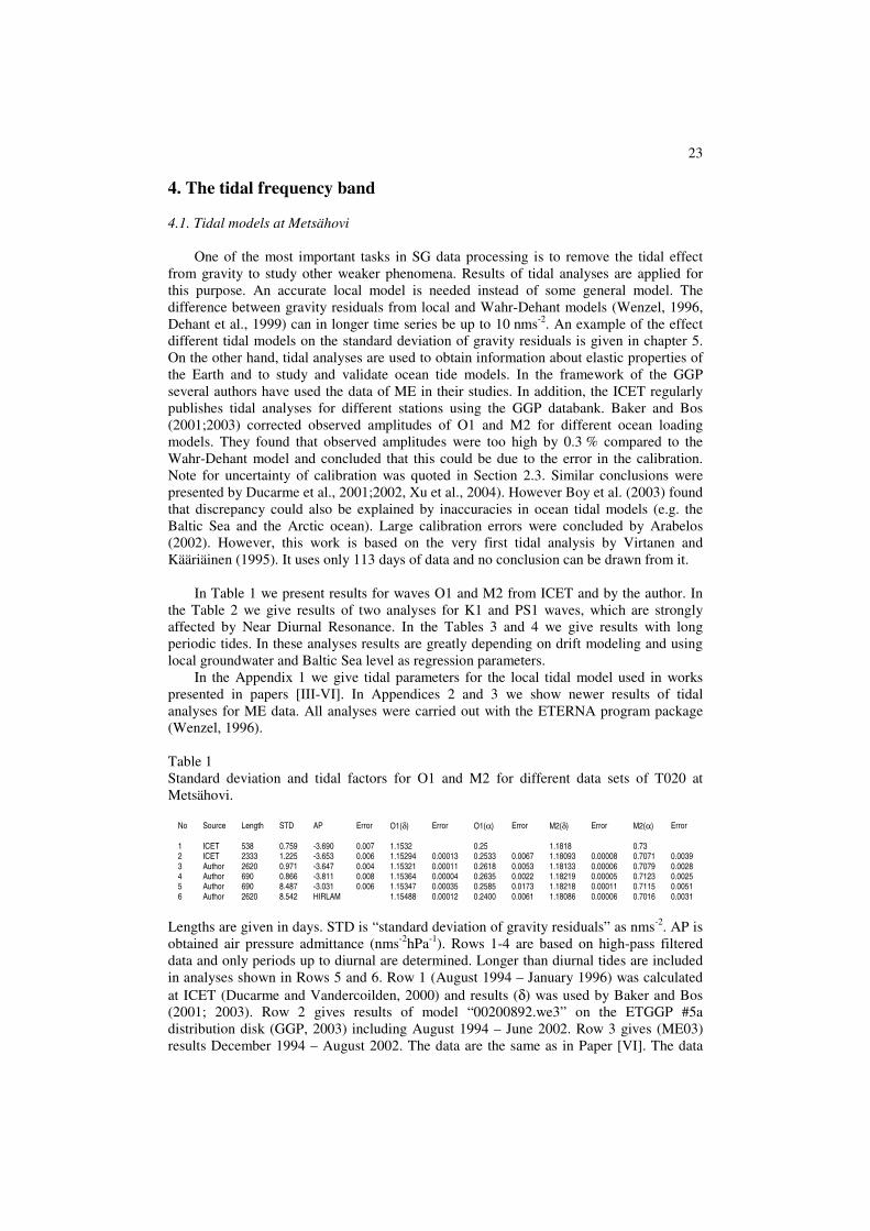
Table 1
Standard deviation and tidal factors for O1 and M2 for different data sets of T020 at
Metsähovi.
No Source Length STD AP Error O1(δ) Error O1(α) Error M2(δ) Error M2(α) Error
1 ICET 538 0.759 -3.690 0.007 1.1532 0.25 1.1818 0.73 2 ICET 2333 1.225 -3.653 0.006 1.15294 0.00013 0.2533 0.0067 1.18093 0.00008 0.7071 0.0039 3 Author 2620 0.971 -3.647 0.004 1.15321 0.00011 0.2618 0.0053 1.18133 0.00006 0.7079 0.0028 4 Author 690 0.866 -3.811 0.008 1.15364 0.00004 0.2635 0.0022 1.18219 0.00005 0.7123 0.0025 5 Author 690 8.487 -3.031 0.006 1.15347 0.00035 0.2585 0.0173 1.18218 0.00011 0.7115 0.0051 6 Author 2620 8.542 HIRLAM 1.15488 0.00012 0.2400 0.0061 1.18086 0.00006 0.7016 0.0031
Lengths are given in days. STD is “standard deviation of gravity residuals” as nms-2
. AP is
obtained air pressure admittance (nms-2
hPa-1
). Rows 1-4 are based on high-pass filtered
data and only periods up to diurnal are determined. Longer than diurnal tides are included
in analyses shown in Rows 5 and 6. Row 1 (August 1994 – January 1996) was calculated
at ICET (Ducarme and Vandercoilden, 2000) and results (δ) was used by Baker and Bos
(2001; 2003). Row 2 gives results of model “00200892.we3” on the ETGGP #5a
distribution disk (GGP, 2003) including August 1994 – June 2002. Row 3 gives (ME03)
results December 1994 – August 2002. The data are the same as in Paper [VI]. The data

24
processing and analyses were made by the author. Fig. 4.1 shows the spectrum of gravity
residuals after this analysis. All tidal parameters are shown in Appendix 3.
Results in Row 4 are based on the same data as Row 5 (November 1994 – October 1996)
and gave the LTM used in Papers [III-VI]. The analysis in Row 5 includes long periodic
tides. However, in the actually used LTM (ME01, Appendix 1) we have used a priori
values (δ=1.16 and α=0.00) for SA and SSA waves.
Row 6 gives results for the same data as used in Row 3, however, including long periodic
tides too. This model is referred as ME02. Air pressure effect was corrected with
HIRLAM, and HSL (Helsinki Sea Level) was used as a meteorological or a hydrological
parameter. The procedure of air pressure corrections is explained in detail in Paper [VI].
Complete results are given in Appendix 2.
Fig 4.1. Amplitude spectrum of gravity residuals for ME03.
Temporal stability of different data sets for tidal factor (δ) are calculated to be < 0.1%,
when comparing two data sets (1994-1996 and 1997-2000) and waves O1, K1, M2 and S2
at ICET (Ducarme et al., 2002)
GGP data has been used for determinations of FCN parameters (Free core nutation).
The obtained eigen periods comprised between 429.1 and 429.9 days, converging towards
value 429.5 days reduced from VLBI observations (Ducarme et al., 2002, Sun, et al.
2002a, Sun, et al. 2002b). For ME the value of 430.6 has been obtained (Sun et al. 2002a).
As an example the Table 2 shows results of two analyses for waves K1 and PSIII. These
waves are strongly affected by the near diurnal resonance.
Table 2
Results (T020) for waves K1 and PSII, which were analysed at
ICET and by author.
No Source K1(δ) Error K1(α) Error PSI1(δ) Error PSI1(α) Error
2 ICET 1.14051 0.00009 0.0695 0.0046 1.25887 0.01096 0.5158 0.4990 3 Author 1.14055 0.00007 0.0793 0.0036 1.25783 0.00868 0.4927 0.3954
25
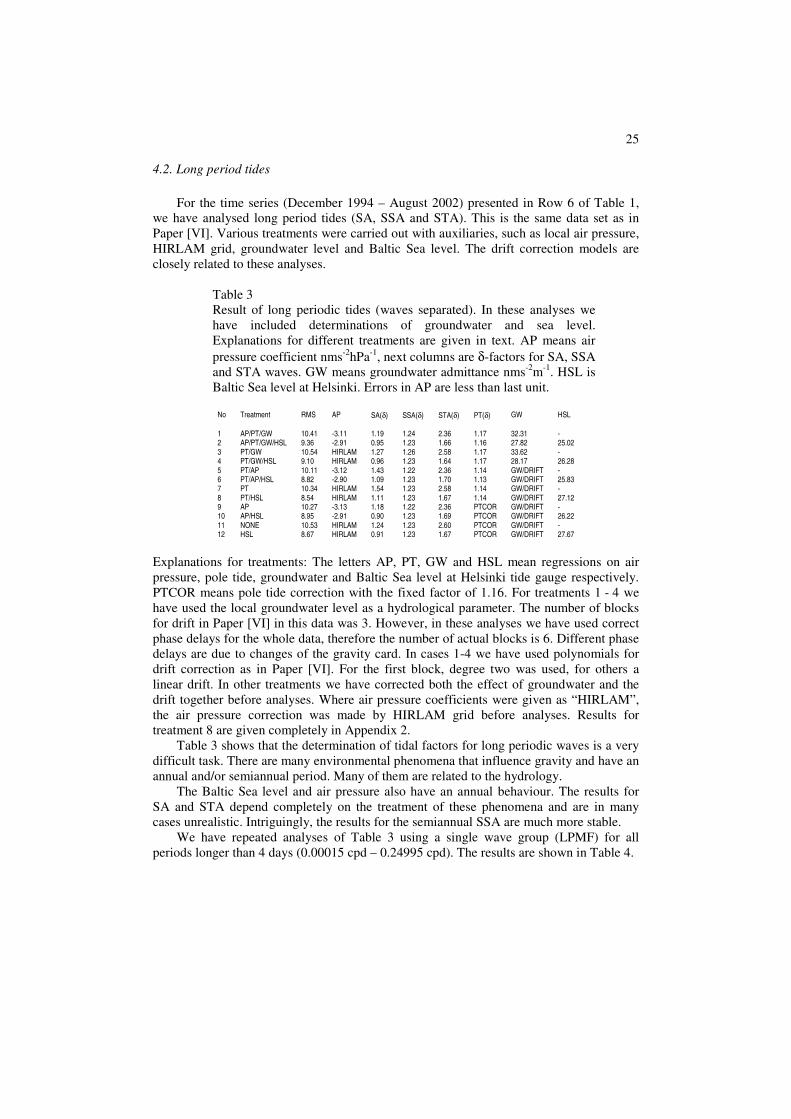
4.2. Long period tides
For the time series (December 1994 – August 2002) presented in Row 6 of Table 1,
we have analysed long period tides (SA, SSA and STA). This is the same data set as in
Paper [VI]. Various treatments were carried out with auxiliaries, such as local air pressure,
HIRLAM grid, groundwater level and Baltic Sea level. The drift correction models are
closely related to these analyses.
Table 3
Result of long periodic tides (waves separated). In these analyses we
have included determinations of groundwater and sea level.
Explanations for different treatments are given in text. AP means air
pressure coefficient nms-2
hPa-1
, next columns are δ-factors for SA, SSA
and STA waves. GW means groundwater admittance nms-2
m-1
. HSL is
Baltic Sea level at Helsinki. Errors in AP are less than last unit.
No Treatment RMS AP SA(δ) SSA(δ) STA(δ) PT(δ) GW HSL
1 AP/PT/GW 10.41 -3.11 1.19 1.24 2.36 1.17 32.31 - 2 AP/PT/GW/HSL 9.36 -2.91 0.95 1.23 1.66 1.16 27.82 25.02 3 PT/GW 10.54 HIRLAM 1.27 1.26 2.58 1.17 33.62 - 4 PT/GW/HSL 9.10 HIRLAM 0.96 1.23 1.64 1.17 28.17 26.28 5 PT/AP 10.11 -3.12 1.43 1.22 2.36 1.14 GW/DRIFT - 6 PT/AP/HSL 8.82 -2.90 1.09 1.23 1.70 1.13 GW/DRIFT 25.83 7 PT 10.34 HIRLAM 1.54 1.23 2.58 1.14 GW/DRIFT - 8 PT/HSL 8.54 HIRLAM 1.11 1.23 1.67 1.14 GW/DRIFT 27.12 9 AP 10.27 -3.13 1.18 1.22 2.36 PTCOR GW/DRIFT - 10 AP/HSL 8.95 -2.91 0.90 1.23 1.69 PTCOR GW/DRIFT 26.22 11 NONE 10.53 HIRLAM 1.24 1.23 2.60 PTCOR GW/DRIFT - 12 HSL 8.67 HIRLAM 0.91 1.23 1.67 PTCOR GW/DRIFT 27.67
Explanations for treatments: The letters AP, PT, GW and HSL mean regressions on air
pressure, pole tide, groundwater and Baltic Sea level at Helsinki tide gauge respectively.
PTCOR means pole tide correction with the fixed factor of 1.16. For treatments 1 - 4 we
have used the local groundwater level as a hydrological parameter. The number of blocks
for drift in Paper [VI] in this data was 3. However, in these analyses we have used correct
phase delays for the whole data, therefore the number of actual blocks is 6. Different phase
delays are due to changes of the gravity card. In cases 1-4 we have used polynomials for
drift correction as in Paper [VI]. For the first block, degree two was used, for others a
linear drift. In other treatments we have corrected both the effect of groundwater and the
drift together before analyses. Where air pressure coefficients were given as “HIRLAM”,
the air pressure correction was made by HIRLAM grid before analyses. Results for
treatment 8 are given completely in Appendix 2.
Table 3 shows that the determination of tidal factors for long periodic waves is a very
difficult task. There are many environmental phenomena that influence gravity and have an
annual and/or semiannual period. Many of them are related to the hydrology.
The Baltic Sea level and air pressure also have an annual behaviour. The results for
SA and STA depend completely on the treatment of these phenomena and are in many
cases unrealistic. Intriguingly, the results for the semiannual SSA are much more stable.
We have repeated analyses of Table 3 using a single wave group (LPMF) for all
periods longer than 4 days (0.00015 cpd – 0.24995 cpd). The results are shown in Table 4.

26
Table 4
Results for long periodic tide LPMF.
No Treatment RMS AP LPMF(δ) Phase(α) PT GW HSL
1 AP/PT/GW 10.88 -3.13 1.16356±0.00326 0.0178±0.1613 1.18±0.34 29.9±0.1 -
2 AP/PT/GW/HSL 9.80 -2.91 1.16276±0.00279 -0.3438±0.1386 1.16±0.29 28.1±0.1 23.7±0.2 3 PT/GW 11.11 HIRLAM 1.16517±0.00302 0.1889±0.1487 1.18±0.32 30.8±0.1 -
4 PT/GW/HSL 9.53 HIRLAM 1.16351±0.00252 -0.3259±0.1254 1.16±0.27 28.3±0.1 25.2±0.2 5 PT/AP 10.58 -3.14 1.16227±0.00327 0.0319±0.1616 1.14±0.31 GW/DRIFT -
6 PT/AP/HSL 9.21 -2.90 1.16221±0.00279 -0.2908±0.1380 1.14±0.27 GW/DRIFT 25.6±0.2 7 PT 10.89 HIRLAM 1.16352±0.00300 0.1778±0.1477 1.13±0.29 GW/DRIFT -
8 PT/HSL 8.94 HIRLAM 1.16285±0.00252 -0.2810±0.1248 1.14±0.24 GW/DRIFT 26.9±0.2 9 AP 10.66 -3.15 1.16041±0.00325 0.0210±0.1607 PTCOR GW/DRIFT -
10 AP/HSL 9.38 -2.91 1.15995±0.00274 -0.2910±0.1357 PTCOR GW/DRIFT 24.9±0.2 11 NONE 10.99 HIRLAM 1.16166±0.00299 0.1624±0.1472 PTCOR GW/DRIFT -
12 HSL 9.10 HIRLAM 1.16067±0.00250 -0.2809±0.1238 PTCOR GW/DRIFT 26.6±0.2
Residuals and amplitude factors are smaller using sea level corrections, and the phases
change sign. Residuals are generally greater than in Table 3 (≈5%). A similar study of long
period tides was made by Ducarme et al.(2004). They get for LPMF 1.15246±0.00317(δ)
and 0.302±0.157(α). After the ocean load correction their results are 1.16945±0.00317(δ)
and -0.427±0.157(α). Our values (without ocean load correction) are clearly larger.
However, Ducarme et al. (2004) do not take into account groundwater or the Baltic Sea. If
we do not correct groundwater in treatment no 1 we get δ = 1.15268 (±0.00378), which is
very close to Ducarme et al. (2004), This shows the importance of environmental
parameters even in the LPMF approach.
5. Atmospheric effects and the Baltic Sea loading
5.1. Single admittance for air pressure and modeled Baltic Sea
The Paper [V] concerns the effect of the Baltic Sea on gravity at ME. The station is 10
km from the nearest bay of the Baltic Sea and 15 km from the open sea. The tidal variation
is of the order of centimeters only, but non-tidal variation of the Baltic is large, up to 2-3 m
on the coasts of the Gulf of Bothnia and the Gulf of Finland. Sea level variations in the
Baltic are driven at short periods primarily by wind stress, and at longer periods by water
exchange through the Danish straits. The loading effect of the Baltic Sea is immediately
recognizable in the gravity record of the T020, by simply inspecting residual gravity
together with the tide gauge record at Helsinki 30 km away ([V], Fig. 5). Loading
calculations show that a uniform layer of water covering the complete Baltic Sea increases
the gravity in Metsähovi by 31 nm/s2 per 1 m of water, and the vertical deformation is
-11 mm. We get regression coefficient for short time series (from 6 January to 5 May
2000) 28.8±0.4 nms-2
m-1
, with the correlation coefficient 0.83.
For the whole data (1994-2001) the regression coefficient is 16.6±0.2 nms-2
m-1
, with
correlation 0.26. RMS of gravity residuals decreases from 16.6 to 14.0 nms-2
. In addition,
we calculated the loading effect of the Baltic Sea in ME for 75 models of momentary sea
surface (November 15, 2001 – January 27, 2002), using data of 11 tide gauges around the
Baltic Sea. For these modelled effects the regression coefficient was 15.7 nms-2
m-1
. This
study was presented as one of the scientific achievements of the first phase of the GGP
(Hinderer and Crossley, 2004).

27
5.2. Air pressure grid and single tide gauge
In the Paper [VI] we used a longer time series for gravity (1994-2002). This data was
completely reprocessed. In the calculation of the air pressure effect, beside local
barometer, we have used a grid model (HIRLAM) for air pressure. Regression of gravity
residuals on the tide gauge record at Helsinki (at 30 km distance) gives a gravity effect of
26 nms-2
m-1
for the Baltic loading. The correlation coefficient was 0.56. The Paper [VI]
demonstrates usefulness of using a grid for a larger area in addition to the local barometer.
5.3. Vertical motion due to loading and GPS
The gravity station is co-located with a permanent GPS station. We have also
associated the loading effects of the atmosphere and of the Baltic Sea with temporal height
variations. The range of air pressure variations is 100 hPa (940 – 1040 hPa) and the mean
is 1004 hPa. The range of modelled vertical motion due to air pressure was 46 mm and that
due to sea level 18 mm. The total range was 38 mm. The effects of the Baltic Sea and of
the atmosphere partly cancel each other, since at longer periods the inverse barometer
assumption is valid. Regression of the modelled height on local air pressure gives
-0.37 mm hPa-1
, corresponding approximately to width 6° for pressure system, which is
imposed on the actual land-sea geometry of Scandinavia (Scherneck, 1994).
We have tested the models using one year of daily GPS data. Multilinear regression
on local air pressure and sea level in Helsinki gives the coefficient -0.34 mm hPa-1
for
pressure, and -11 mm m-1
for sea level. These match model values. Loading by air
pressure and Baltic Sea explains nearly 40 % of the variance of daily GPS height
solutions.
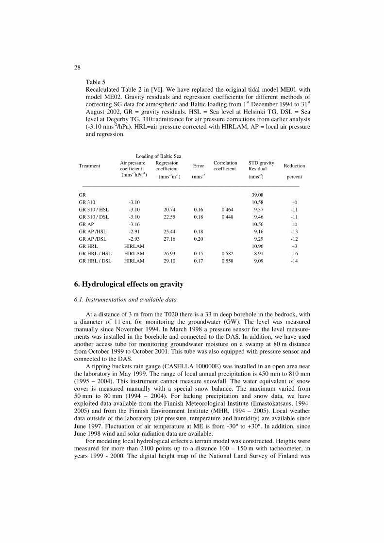
5.4. The effects of different tidal models
Table 5 gives results of new studies correcting gravity for atmospheric and Baltic
loading. The table is the similar to Table 2 [VI], but we demonstrate the effect of a
different tidal model used in the pre-processing. We have replaced the tidal model ME01
(Appendix 1) originally used with the new model ME02 (Appendix 2). See Section 4.1.
Comparing to the reference GR310, we have reduced residuals (GR HRL /HSL) 16%.
Using the original tidal model (ME01), the reference RMS was 10.91 nms-2
. Using this
reference, the reduction is 18%. For model ME02 we have corrected air pressure effect by
HIRLAM grid and used Helsinki tide gauge as a hydrological regression parameter. Drift
correction was made before analysis using polynomial fit together with groundwater [VI].
For comparison, using Wahr-Dehant models (Wenzel, 1996, Dehant et al., 1999), the RMS
of gravity (GR310) is 12.94 nms-2
. Examples demonstrate the importance of accuracy of
the local tidal model used.
28
Table 5
Recalculated Table 2 in [VI]. We have replaced the original tidal model ME01 with
model ME02. Gravity residuals and regression coefficients for different methods of
correcting SG data for atmospheric and Baltic loading from 1st December 1994 to 31
st
August 2002, GR = gravity residuals. HSL = Sea level at Helsinki TG, DSL = Sea
level at Degerby TG, 310=admittance for air pressure corrections from earlier analysis
(-3.10 nms-2
/hPa). HRL=air pressure corrected with HIRLAM, AP = local air pressure
and regression.
Loading of Baltic Sea
Treatment Air pressure
coefficient
Regression
coefficient Error
Correlation
coefficient
STD gravity
Residual Reduction
(nms-2hPa-1) (nms-2m-1) (nms-2 (nms-2) percent
____________________________________________________________________________________
GR 39.08
GR 310 -3.10 10.58 ±0
GR 310 / HSL -3.10 20.74 0.16 0.464 9.37 -11
GR 310 / DSL -3.10 22.55 0.18 0.448 9.46 -11
GR AP -3.16 10.56 ±0
GR AP /HSL -2.91 25.44 0.18 9.16 -13
GR AP /DSL -2.93 27.16 0.20 9.29 -12
GR HRL HIRLAM 10.96 +3
GR HRL / HSL HIRLAM 26.93 0.15 0.582 8.91 -16
GR HRL / DSL HIRLAM 29.10 0.17 0.558 9.09 -14
6. Hydrological effects on gravity
6.1. Instrumentation and available data
At a distance of 3 m from the T020 there is a 33 m deep borehole in the bedrock, with
a diameter of 11 cm, for monitoring the groundwater (GW). The level was measured
manually since November 1994. In March 1998 a pressure sensor for the level measure-
ments was installed in the borehole and connected to the DAS. In addition, we have used
another access tube for monitoring groundwater moisture on a swamp at 80 m distance
from October 1999 to October 2001. This tube was also equipped with pressure sensor and
connected to the DAS.
A tipping buckets rain gauge (CASELLA 100000E) was installed in an open area near
the laboratory in May 1999. The range of local annual precipitation is 450 mm to 810 mm
(1995 – 2004). This instrument cannot measure snowfall. The water equivalent of snow
cover is measured manually with a special snow balance. The maximum varied from
50 mm to 80 mm (1994 – 2004). For lacking precipitation and snow data, we have
exploited data available from the Finnish Meteorological Institute (Ilmastokatsaus, 1994-
2005) and from the Finnish Environment Institute (MHR, 1994 – 2005). Local weather
data outside of the laboratory (air pressure, temperature and humidity) are available since
June 1997. Fluctuation of air temperature at ME is from -30° to +30°. In addition, since
June 1998 wind and solar radiation data are available.
For modeling local hydrological effects a terrain model was constructed. Heights were
measured for more than 2100 points up to a distance 100 – 150 m with tacheometer, in
years 1999 - 2000. The digital height map of the National Land Survey of Finland was
29
used (25 m grid) beyond this area. The detection threshold of transient gravity changes for
SG is about a nms-2
corresponding 2 mm water as Bouguer approximation. The calculated
gravity effect of a 10 mm water layer on the surface for area 200 × 200 m around the SG is
1.2 nms-2
excluding the building area. For a larger area 1 ×1 km we get only a 0.2 nms-2
more. The calculated total effect is thus 1/3 of the Bouguer plate approximation. We
should expect detectable effects (about 3 nms-2
) in gravity for a sudden shower of 10 mm
and 7-11 nms-2
maximally for the snow cover.
To estimate soil moisture effects, the thickness of soil above bedrock was determined
with gravimetric techniques and by drilling up to a distance 100 m. The mean soil
thickness around the laboratory is 0.75 m and the maximum 3.8 m. Calculations show that
a change by 10 % in the moisture content of the soil (mossy moraine) changes gravity by
8 nms-2
.
6.2. Results of local studies
The Papers [III and IV] present results of hydrological studies with T020 at ME. The
Paper [III] presents first results of clear correlation between SG gravity and groundwater
level for years 1994 - 1999. This effect was found earlier with relative gravimeter by
Mäkinen and Tattari (1990, 1991) and with SG by Peter et al. (1995). In the Paper [IV] we
confirmed the effect of GW on the gravity from December 1994 to August 2000. We got
an admittance for GW, 27 nms-2
m-1
that is still usable. The RMS of gravity residuals
reduced from 21 nms-2
to 14 nms-2
. Using a simple Bouguer-plate approximation, we get a
specific yield of 7 %, which is high compared with the porosity of monolithic granite (1-
2 %). Obviously, the water is contained in the fractures of rock. It is likely that the level in
the well also acts as an indicator for the water in the sediments.
An important discovery was the effect of snow cover on the roof of the laboratory. It
was found experimentally by chance. A heavy load of snow (23000 kg) was dropped from
the roof. The change in gravity was +23 nms-2
. Fortunately we had measured the properties
of snow load some days before. Modeling calculations confirmed the observed results. Our
recommendations for SG stations were: monitoring groundwater level, measurements of
water equivalent of snow at least up to a distance of 50 m, terrain modeling and rain gauge.
For detailed investigations an additional access tube was used to monitor groundwater
in the soil. The water level correlates with the level in the borehole. We have observed that
heavy local precipitation has an immediate influence on gravity through surface soil
moisture. Its impact on groundwater in the borehole is smoother and delayed by some
hours (Fig. 4, [IV] and Hokkanen et al. (2004, 2005). Some observations suggest that a
sudden 20 mm precipitation increases temporarily gravity by about 10 nms-2
or more
compared to the surface area model mentioned in Section 6.1. Presumably, a neighbouring
area acts as a temporary reservoir. Local hydrology includes still open questions and is an
object of recent studies.
We usually correct the effect of groundwater at the preprocessing stage together with
the drift correction. Similar values for GW admittance are formed in tidal analyses (27-
28 nms-2
m-1
). The GW level 1994 – 2004 is shown in Fig. 6.1. Its range is 2.3 meters and
the minimum level is about 8 meters below the SG. In Fig 6.1 we have removed from
gravity data tides, pole tide and effect of air pressure (-3.10 nms-2
hPa-1
). A fit between
gravity residuals and GW gives 27.4 nms-2
m-1
with correlation coefficient 0.79 (Fig. 6.1).

30
6.3. Regional and global hydrology
The papers [III, IV] treat only the local hydrology and the Newtonian attraction due to
it. We have recently extended these studies to include regional and global water storage
and its loading effect i.e. both the vertical deformation and the Newtonian attraction. We
used two hydrological models: The Climate Prediction Center global soil moisture data set
(Fan et al., 2004) and the Watershed Simulation and Forecasting System (WSFS) of the
Finnish Environment Institute (Vehviläinen, et al., 2002). We have compared (Virtanen et
al. 2005a; 2005b) the time series of T020 with both, using regression methods and loading
calculations. A key question is the separation of the attraction of near-field water storage
from the loading effect of the regional water storage, as the two are strongly correlated. A
likely outcome of the study is revision of the admittance of the local groundwater level
into gravity at ME (previous section).
Hydrological phenomena appear to be a main cause for the regional gravity variation
detected by the gravity satellites CHAMP and GRACE. In several studies (Crossley and
Hinderer, 2002; Crossley et al., 2005; Neumeyer et al. 2004; 2006; Virtanen et al. 2005a;
2005b) a correlation between regional gravity variation detected by the satellites and point
gravity variation detected by the SGs has been pointed out. The question is again, which
part of the SG response is driven by the regional hydrological loading and which part by
the local hydrological attraction. A more detailed discussion is outside the scope of this
study.
Fig. 6.1. Gravity and groundwater level at Metsähovi 1.12.1994 – 17.4.2004. Top:
Groundwater level below surface, with the range of 2 meters. Bottom: Gravity residual and
fitted groundwater level, the regression coefficient is 27.4 nms-2
m-1
with correlation
coefficient 0.79.

31
7. Summary and conclusions
Results of studies of Earth dynamics with the superconducting gravimeter T020 were
presented from 1994 to 2005. The new data acquisition system developed by the author
was described in detail. The new system has been proved to be reliable and flexible.
Significantly, the accuracy of data and timing system are sufficient for SG. The health of
the whole installation of T020 can be detected via an Internet connection.
Metsähovi belongs to the group of low noise SG stations and is thus suitable for
studies in seismic frequency band. Information on the nature of microseism at Metsähovi
was presented. Annual variations, spectral distributions, amplitudes and sources were
given. There is a clear correlation between the occurrence of a low atmospheric pressure
(storm) in the Northern Atlantic Ocean and microseism.
Free oscillation phenomena of the Earth excited by great earthquakes were
investigated. Spectra, studies of attenuation and rotational splitting were presented. All the
lowest modes of different oscillation types are found (0S2, 0T2 and 0S0). The strongest
earthquake (Mw 9.0) ever observed with T020 happened in Sumatra on December 26,
2004. The amplitude of ground motion due to mode 0S0 was a few days after quake about
0.05 mm, exceeding 10 times that of a strong microseism. This mode was clearly
detectable still 3 months after the earthquake. A special phenomenon is incessant
excitation of the Earth’s free oscillation. The amplitude is on the order of 1 ngal. The
detection of this oscillation with T020 was shown from August 1994 to August 1998.
With the T020 the precise local tidal parameters were determined. The importance of
accuracy of local tidal model used in the data analyses was demonstrated. Hydrological
effects on gravity such as variation in groundwater level, precipitation, soil moisture and
snow cover were studied. The variation in the local groundwater level correlates
significantly (0.79) with gravity. The range was about 2 m and the regression coefficient
27 nms-2
m-1
. This phenomenon was taken into account in an early stage in the data
processing. One important finding was that the local snow cover affects notably on gravity.
We have computed the effects of the variation in atmospheric mass, and of the loading
by the Baltic Sea in gravity. Examinations utilize both regression methods based on a
single tide gauge/barometer, and calculations with detailed models for the surface loads.
Theoretical loading calculations using Green’s functions formalism were performed for
both vertical motion and gravity. A uniform layer of water covering the complete Baltic
Sea increases the gravity at Metsähovi by 31 nms-2
m-1
and the vertical deformation is
-11 mm. Regressing the gravity residual for 1994 – 2002 on the nearest tide gauge at
Helsinki gave the coefficient 26.9 nms-2
m-1
, which is 87% of the model value for a uniform
layer of water. Loading studies were associates with temporal height variations using the
GPS data of Metsähovi permanent station. Loading by air pressure and the Baltic Sea
explains about 40% of the variance of daily GPS height solution.
Results of long time series at Metsähovi demonstrated high quality of data and
correctly carried out offsets and drift corrections. The superconducting gravimeter T020
has been proved to be an eminent and versatile tool in studies of the Earth dynamics.
32
References
Arabelos, D., 2002. Comparison of Earth-tide parameters over a large latitude difference.
Geophys. J. Int. 151, 950-956.
Baker, T. and Bos, M., 2001. Tidal Gravity Observations and Ocean Tide Models. J.
Geod. Soc. Japan 47 (1), 76-81.
Baker, T. and Bos, M., 2003. Validating Earth and ocean tide models using tidal gravity
measurements. Geophys. J. Int. 152, 468-485.
Banka, D., 1997. Noise levels of superconducting gravimeters at seismic frequencies, PhD
thesis, GDMB-Informationgesellschaft mbH, Clausthal, Germany.
Banka, D. and Crossley, D.J., 1999. Noise levels of superconducting gravimeters at
seismic frequencies, Geophys. J. Int. 139, 87-97.
Boy, J.-P., M. Llubes, J. Hinderer, and N. Florsch, 2003. A comparison of tidal ocean
loading models using superconducting gravimeter data. J. Geophys. Res. 108 (B4),
2193, doi: 10.1029/2002JB002050.
Crossley, D., Hinderer, J., Casula, G., Francis, O., Hsu, H.-T., Imanishi, Y., Jentzsch, G.,
Kääriäinen, J., Merriam, J., Meurers, B., Neumeyer, J., Richter, B., Shibuya, K., Sato,
T. and van Dam, T., 1999. Network of superconducting gravimeters benefits a number
of disciplines. Trans. Am. Geophys. U. 80, 121–126.
Crossley, D., and Hinderer, J., 2002. GGP Ground Truth for Satellite Gravity Missions.
Bull. d'Inf. Marées Terr. 136, 10735-10742.
Crossley, D., Hinderer, J., Boy, J-P., 2004. Regional gravity variations in Europe from
superconducting gravimeters. J. Geodyn. 38 (3-5), 325-342.
Crossley, D., Hinderer, J., Boy, J-P., 2005. Time variations of the European gravity field
from superconducting gravimeter. Geophys. J. Int., 161, 257-264.
Dehant, V., Defraigne, P., Wahr, J., 1999. Tides for a convective Earth. J. Geophys. Res.
104 (B1), 1035-1058.
Ducarme, B, Vandercoilden, L., 2000. First Results of the GGP data Bank At
ICET, Cahiers du Centre Européen de Géodynamique et de Séismologie 17, 117-124.
Ducarme, B. and Sun, H.-P., 2001. Tidal gravity results from GGP network in connection
with tidal loading and Earth response, J. Geod. Soc. Jap. 47 (1), 308-315.
Ducarme, B., Sun, H.-P., Xu, J.-Q., 2002. New investigations of tidal gravity results from
the GGP network, Bull. d'Inf. Marées Terr. 136, 10761-10766.
Ducarme, B., Venedikov, A., Arnoso, J., Vieira, R., 2004. Determination of the long
period tidal waves in the GGP superconducting gravity data. J. Geodyn. 38 (3-5), 307-
324.
Dunn, B., 1994. CSGI Software Reference Manual, Revision 3.1. Dept. Earth Sciences,
The University of Western Ontario, London, Ontario, Canada.
Fan, Y., Van den Dool, H. ,2004. The CPC global monthly soil moisture data set at 1/2
degree resolution for 1948-present. J. Geophys. Res. 109, D10102,
doi: 10.1029/2003JD004345.
GGP, 2003. CD-ROM ETGGP #5A, The GGP consortium. http://ggp.gfz-potsdam.de/.
GGP, 2006. GGP Home Page. http://www.eas.slu.edu/GGP/ggphome.html.
Goodkind, J., 1999. The superconducting gravimeter, Review of Scientific Instruments 70
(11), 4131-4152.
GWR, 1989. Superconducting gravity meter, Operational Manual, Serie #019, San Diego,
USA.
33
Hinderer, J., Amalvict, M., Francis, O. and Mäkinen, J., 1998. On the calibration of super-
conducting gravimeters with the help of absolute gravity measurements, in: Proc. 13th
Int. Symp. Earth Tides, Brussels 1997, 557-564, Observatoire Royal de Belgique.
Hinderer, J., Crossley, D., 2000. Time variations in gravity and inferences on the Earth’s
structure and dynamics. Surveys in Geophysics 21, 1–45.
Hinderer, J., Crossley, D., 2004. Scientific achievements from the first phase (1997-2003)
of the Global Geodynamics Project using a worlwide network of supeconducting
gravimeters. J. Geodyn. 38 (3-5), 237-262.
Hokkanen, T., Virtanen, H., Pirttivaara, M.,2004. Groundwater, soil moisture, and
superconducting gravimeter data. European Association of Geoscientists and Engineers
(EAGE), 66th
Conference and Exhibition, Paris, 7–10 June, 2004. Abstract and poster.
Hokkanen, T., Virtanen, H., Pirttivaara, M., 2005. On the hydrogeological noise in
superconducting gravimeter data. Submitted to Near Surface Geophysics.
Ilmastokatsaus, 1994–2005. Finnish Meteorological Institute, (Monthly survey in Finnish).
Jentzsch, G., Crossley, D., Hinderer, J., Takemoto, S., 2004. Time varying gravimetry,
GGP and vertical motions J. Geodyn. 38 (3-5).
MHR, 1994-2005. Monthly Hydrological Report, Finnish Environment Institute,
Hydrology and Water Management Division, 1994 – 2005, Helsinki.
Mäkinen, J., Tattari, S., 1990. The influence of variation in subsurface water storage on
observed gravity, Proc. 11th Int. Symp. Earth Tides, ed. J. Kakkuri, Schweitzerbart.
Verlag, Stuttgart, 457-471.
Mäkinen, J., Tattari, S., 1991. Subsurface water and gravity, in Proceedings of the
Workshop: Non Tidal Gravity Changes Intercomparison between absolute and
superconducting gravimeters. Ed. Poitevin, C., Cahiers du Centre Européen de
Géodynamique et de Séismologie 3, 235-240.
Mäkinen, J., Kääriäinen, J., Virtanen, H. ,1995. Calibration of a superconducting
gravimeter using short sets of simultaneous observations with an absolute gravimeter.
Poster presented at XXI General Assembly of IUGG in Boulder, USA.
Nawa, K., Suda, N., Fukao, Y., Sato, T., Aoyama, Y., Shibuya, K., 1998. Incessant
excitation of the Earth's free oscillations, Earth, Planets and Space, 50 (1), 3-8.
Nawa, K., Suda, N., Fukao, Y., Sato, T., Tamura, Y., Shibuya, K., McQueen, H., Virtanen,
H., Kääriäinen, J., 2000. Incessant excitation of the Earth’s free oscillations: global
comparison of superconducting gravimeter records, Phys. Earth planet. Int. 120, 289-
297.
NEIC, 2005. National Earthquake Information Center. USGS Earthquake Hazards
Program web site: http://wwwneic.cr.usgs.gov/.
Neumeyer, J., Schwintzer, P., Barthelmes, F., Dierks,O., Imanishi, Y., Kroner, C.,
Meurers, B., Sun, H.-P., Virtanen, H., 2004. Comparison of Superconducting
Gravimeter and CHAMP Satellite Derived Temporal Gravity Variations. Ed. C.
Reigber et. Al. Earth Observations with Champ, Results from Three Years in Orbit.
Springer, 31-36.
Neumeyer, J., Barthelmes, F., Dierks, O., Flechtner, F., Harnisch, M., Harnisch, G.,
Hinderer, J., Imanishi, Y., Kroner, C., Meurers, B., Petrovic, S., Reigber, Ch., Schmidt,
R., Schwintzer, P., Sun,H.-P., Virtanen, H., 2006. Combination of temporal gravity
variations resulting from Superconducting Gravimeter recordings, GRACE satellite
observations and global hydrology models. J. Geodesy, doi: 10.1007/S00190-005-
0014-8.
Peter, G., Klopping, F.J., Berstis, K.J., 1995. Observing and Modeling Gravity Changes
Caused by Soil Moisture and Groundwater Table Variations with Superconducting
Gravimeters in Richmond, Florida, U.S.A, Cahiers du Centre Européen de
Géodynamique et de Séismologie 11, 147-158.
34
Peterson, J., 1993. Observations and modelling of seismic background noise. Open-File
report 93-332, U.S.Department of Interior, Geological Survey, Albuquerque, New
Mexico.
Prothero, W.A., Goodkind, J., 1968. A superconducting gravimeter. Rev. Sci. Instr. 39 (9),
1257–1268.
Rosat, S., Hinderer, J. and D. Crossley, 2002. A comparison of the seismic noise levels at
various GGP stations, Bull. d´Inf. Marées Terr. 135, 10689-10700.
Rosat, S., Hinderer, J., Crossley, D., and J. P. Boy, 2004. Performance of superconducting
gravimeters from long period seismology to tides. J. Geodyn. 38 (3-5), 461-476.
Scherneck, H.-G., 1994. Realistic modelling of deformations due to air pressure variations.
In: Harsson, B.G., Ness, J.A., (Eds.), Proceedings of the 12th General Meeting of the
Nordic Geodetic Commission, Ullensvang, Norway, 30 May – 3 June 1994, 229-243.
Smylie, D., Francis, O., Merriam, J.,2001. Beyond tides-determinations of core properties
from superconducting gravimeter observations. J. Geodet. Soc. Japan 47 (1), 364-372.
Sun, H.-P., Hsu, H.-T., Jentzsch, G., and Xu, J.-Q., 2002a. Tidal gravity observations
obtained with a superconducting gravimeter at Wuhan/China and its application to
geodynamics, J. Geodyn. 33 (1-2), 187-198.
Sun, H.-P., Xu, J-Q, and Ducarme, B., 2002b. Preliminary results of the Free Core
Nutation eigenperiod obtained by stacking SG observations at GGP stations, Bull.
d'Inf. Marées Terr. 136, 10725-10728.
Van Camp, M., Wenzel, H.-G., Schott, P., Vauterin, P. and Francis, O., 2000. Accurate
transfer function determination for superconducting gravimeters. Geophys. Res. Let. 27
(1), 37-40.
Van Camp, M., and Vauterin, P., 2005. Tsoft: graphical and interactive software for the
analysis of time series and Earth tides, Computers & Geosciences 31 (5), 631-640.
Van Dam, T.M. and Wahr, J., 1998. Modeling environment loading effects: a Review.
Phys. Chem. Earth 23 (9–10), 1077–1087.
Vehviläinen, B. and Huttunen, M., 2002. The Finnish watershed simulation and
forecasting system (WSFS). XXI Conference of the Danubian countries on the
hydrological forecasting and hydrological bases of water management. Bucharest,
Romania. 2-6 September 2002.
Virtanen, H., Kääriäinen, J., 1995. The installation of and first results from the
superconducting gravimeter GWR20 at the Metsähovi station, Finland. Rep. Finn.
Geod. Inst. 95:1, 1–15.
Virtanen, H., Kääriäinen, J., 1997. The GWR T020 superconducting gravimeter 1994–
1996 at the Metsähovi station, Finland. Rep. Finn. Geod. Inst. 97:4, 1–26.
Virtanen, H., Mäkinen, J. , 2003: Air pressure and Baltic Sea loading corrections to gravity
data at Metsähovi. In: Poutanen, M. Suurmäki, H. (Eds), Proceedings of the XIV
General Meeting of the Nordic Geodetic Commission. 148-153.
Virtanen, H., Bilker, M., Mäkinen, J., Poutanen, M, Tervo, M., Vehviläinen, B., Huttunen,
M., Mäkinen, R., 2005a. Comparison of modeled variation in water storage in Finland
with GRACE and superconducting gravimeter observations. Geophysical Research
Abstracts 7, 06248, 2005.
Virtanen, H., Bilker, M., Mäkinen, J., Tervo, M., Vehviläinen, B., Huttunen, M, Mäkinen,
R., Peltoniemi, M., Hokkanen, T., Pirttivaara, M., 2005b. Comparison of modelled
variation in water storage in Finland with superconducting gravimeter observations and
with GRACE. Abstract in Dynamic Planet, Cairns, Australia, 22-26 August 2005.
Warburton, R. J. and Brinton, E.W., 1995. Recent developments in GWR Instruments'
superconducting gravimeters, in Proceedings of Second Workshop: Non-tidal gravity
changes Intercomparison between absolute and superconducting gravimeters, 11, 23-
56, Cahiers du Centre Européen de Géodynamique et de Séismologie 11, 23-56.
35
Wenzel H.-G. ,1996. The nanogal software: earth tide data processing package ETERNA
3.30, Bull. d´Inf. Marées Terr. 124, 9425-9439.
Widmer-Schnidrig, R., 2003. What Can Superconducting Gravimeters Contribute to
Normal –Mode Seismology. Bulletin of the Seismological Society of America 93 (3),
1370-1380.
Xu, J., Sun, H., Ducarme, B., 2004. A global experimental model for gravity tides of the
Earth. Journal of Geodynamics 38 (3-5), 293-306.
Zürn, W., Laske, G., Widmer-Schnidrig, R., and Gilbert, F., 2000. Observations of
Coriolis coupled modes below 1 mHz., Geophys. J. Int. 143, 113-118.

36

37
Appendices

38
Appendix 1
Local tidal model ME01 used in Papers [III-VI]. The format is same as used in the
database for TSOFT program to calculate theoretical tide. The values for SA and SSA are
a priori values. Other factors are based on the analysis (Section 4.1).
Columns are: COMP:, from [cpd], to [cpd], amplitude factor, phase (degree), Wave name.
[TIDECOMP] Metsahovi NAME: ME01 TYPE: 1 AZIM: 0.0000000 GRAV: 0.0000000 COMP: 0.001379 0.004107 1.16000 0.0000 SA COMP: 0.004108 0.020884 1.16000 0.0000 SSA COMP: 0.020885 0.054747 1.14061 1.1762 MM COMP: 0.054748 0.091348 1.15033 -0.1140 MF COMP: 0.091349 0.501369 1.10530 1.2223 MTM COMP: 0.721499 0.851182 1.14121 -3.7435 138 COMP: 0.852095 0.857261 1.12703 -1.0110 2Q1 COMP: 0.857571 0.870022 1.15817 -0.6001 SIG1 COMP: 0.887327 0.894010 1.14475 0.0216 Q1 COMP: 0.895216 0.906314 1.14996 -0.0243 RO1 COMP: 0.921941 0.932582 1.15364 0.2635 O1 COMP: 0.932583 0.940487 1.14979 0.3569 TAU1 COMP: 0.958085 0.968565 1.16256 0.0052 M1 COMP: 0.968565 0.974188 1.15184 0.6248 CHI1 COMP: 0.989048 0.994755 1.14928 0.3137 PI1 COMP: 0.995143 0.998028 1.15501 0.0503 P1 COMP: 0.999852 1.000147 1.08534 6.9280 S1 COMP: 1.001824 1.003651 1.14099 0.0902 K1 COMP: 1.005328 1.005622 1.24159 1.1047 PSI1 COMP: 1.007594 1.011098 1.18278 -0.4384 FI1 COMP: 1.013689 1.034319 1.16873 -0.8384 THE1 COMP: 1.034466 1.044799 1.15238 0.0780 J1 COMP: 1.064841 1.073202 1.17702 0.1981 SO1 COMP: 1.073349 1.080797 1.15405 0.1773 OO1 COMP: 1.080944 1.216396 1.17691 1.3099 V1 COMP: 1.719380 1.827342 1.10910 2.6648 3N2 COMP: 1.827799 1.853920 1.16178 1.4845 EPS2 COMP: 1.854524 1.863634 1.18042 1.4072 2N2 COMP: 1.864090 1.872141 1.16975 0.9096 MI2 COMP: 1.888387 1.900529 1.18165 1.1068 N2 COMP: 1.900544 1.906461 1.18177 1.0229 NI2 COMP: 1.923765 1.942753 1.18219 0.7123 M2 COMP: 1.958232 1.966446 1.16507 0.6909 LMB2 COMP: 1.966446 1.976926 1.17381 0.3273 L2 COMP: 1.991786 1.998287 1.18112 -0.1277 T2 COMP: 1.999705 2.000766 1.17619 0.0376 S2 COMP: 2.002590 2.002885 1.17666 1.9503 R2 COMP: 2.003032 2.031287 1.17797 0.1372 K2 COMP: 2.031434 2.044652 1.16843 0.6820 ETA2 COMP: 2.047243 2.182843 1.16785 -6.8226 2K2 COMP: 2.753243 2.869713 1.07639 0.5531 493 COMP: 2.892640 2.935615 1.08064 0.1416 M3 COMP: 2.940177 3.081253 1.05915 -2.9201 SO3 COMP: 3.791963 3.937896 1.04195 -155.9466 M4
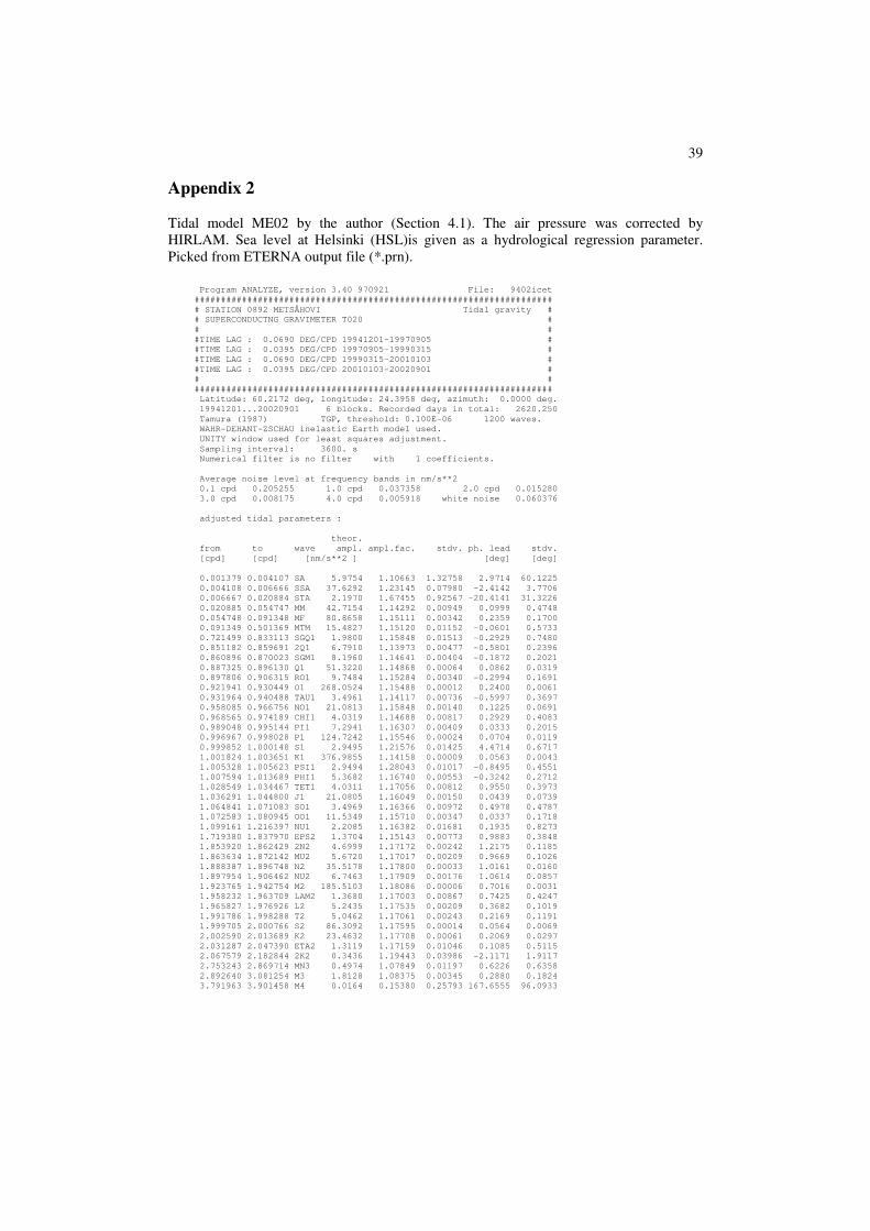
39
Appendix 2
Tidal model ME02 by the author (Section 4.1). The air pressure was corrected by
HIRLAM. Sea level at Helsinki (HSL)is given as a hydrological regression parameter.
Picked from ETERNA output file (*.prn). Program ANALYZE, version 3.40 970921 File: 9402icet #################################################################### # STATION 0892 METSÄHOVI Tidal gravity # # SUPERCONDUCTNG GRAVIMETER T020 # # # #TIME LAG : 0.0690 DEG/CPD 19941201-19970905 # #TIME LAG : 0.0395 DEG/CPD 19970905-19990315 # #TIME LAG : 0.0690 DEG/CPD 19990315-20010103 # #TIME LAG : 0.0395 DEG/CPD 20010103-20020901 # # # #################################################################### Latitude: 60.2172 deg, longitude: 24.3958 deg, azimuth: 0.0000 deg. 19941201...20020901 6 blocks. Recorded days in total: 2620.250 Tamura (1987) TGP, threshold: 0.100E-06 1200 waves. WAHR-DEHANT-ZSCHAU inelastic Earth model used. UNITY window used for least squares adjustment. Sampling interval: 3600. s Numerical filter is no filter with 1 coefficients. Average noise level at frequency bands in nm/s**2 0.1 cpd 0.205255 1.0 cpd 0.037358 2.0 cpd 0.015280 3.0 cpd 0.008175 4.0 cpd 0.005918 white noise 0.060376 adjusted tidal parameters : theor. from to wave ampl. ampl.fac. stdv. ph. lead stdv. [cpd] [cpd] [nm/s**2 ] [deg] [deg] 0.001379 0.004107 SA 5.9754 1.10663 1.32758 2.9714 60.1225 0.004108 0.006666 SSA 37.6292 1.23145 0.07980 -2.4142 3.7706 0.006667 0.020884 STA 2.1970 1.67455 0.92567 -20.4141 31.3226 0.020885 0.054747 MM 42.7154 1.14292 0.00949 0.0999 0.4748 0.054748 0.091348 MF 80.8658 1.15111 0.00342 0.2359 0.1700 0.091349 0.501369 MTM 15.4827 1.15120 0.01152 -0.0601 0.5733 0.721499 0.833113 SGQ1 1.9800 1.15848 0.01513 -0.2929 0.7480 0.851182 0.859691 2Q1 6.7910 1.13973 0.00477 -0.5801 0.2396 0.860896 0.870023 SGM1 8.1960 1.14641 0.00404 -0.1872 0.2021 0.887325 0.896130 Q1 51.3220 1.14868 0.00064 0.0862 0.0319 0.897806 0.906315 RO1 9.7484 1.15284 0.00340 -0.2994 0.1691 0.921941 0.930449 O1 268.0524 1.15488 0.00012 0.2400 0.0061 0.931964 0.940488 TAU1 3.4961 1.14117 0.00736 -0.5997 0.3697 0.958085 0.966756 NO1 21.0813 1.15848 0.00140 0.1225 0.0691 0.968565 0.974189 CHI1 4.0319 1.14688 0.00817 0.2929 0.4083 0.989048 0.995144 PI1 7.2941 1.16307 0.00409 0.0333 0.2015 0.996967 0.998028 P1 124.7242 1.15546 0.00024 0.0704 0.0119 0.999852 1.000148 S1 2.9495 1.21576 0.01425 4.4714 0.6717 1.001824 1.003651 K1 376.9855 1.14158 0.00009 0.0563 0.0043 1.005328 1.005623 PSI1 2.9494 1.28043 0.01017 -0.8495 0.4551 1.007594 1.013689 PHI1 5.3682 1.16740 0.00553 -0.3242 0.2712 1.028549 1.034467 TET1 4.0311 1.17056 0.00812 0.9550 0.3973 1.036291 1.044800 J1 21.0805 1.16049 0.00150 0.0439 0.0739 1.064841 1.071083 SO1 3.4969 1.16366 0.00972 0.4978 0.4787 1.072583 1.080945 OO1 11.5349 1.15710 0.00347 0.0337 0.1718 1.099161 1.216397 NU1 2.2085 1.16382 0.01681 0.1935 0.8273 1.719380 1.837970 EPS2 1.3704 1.15143 0.00773 0.9883 0.3848 1.853920 1.862429 2N2 4.6999 1.17172 0.00242 1.2175 0.1185 1.863634 1.872142 MU2 5.6720 1.17017 0.00209 0.9669 0.1026 1.888387 1.896748 N2 35.5178 1.17800 0.00033 1.0161 0.0160 1.897954 1.906462 NU2 6.7463 1.17909 0.00176 1.0614 0.0857 1.923765 1.942754 M2 185.5103 1.18086 0.00006 0.7016 0.0031 1.958232 1.963709 LAM2 1.3680 1.17003 0.00867 0.7425 0.4247 1.965827 1.976926 L2 5.2435 1.17535 0.00209 0.3682 0.1019 1.991786 1.998288 T2 5.0462 1.17061 0.00243 0.2169 0.1191 1.999705 2.000766 S2 86.3092 1.17595 0.00014 0.0564 0.0069 2.002590 2.013689 K2 23.4632 1.17708 0.00061 0.2069 0.0297 2.031287 2.047390 ETA2 1.3119 1.17159 0.01046 0.1085 0.5115 2.067579 2.182844 2K2 0.3436 1.19443 0.03986 -2.1171 1.9117 2.753243 2.869714 MN3 0.4974 1.07849 0.01197 0.6226 0.6358 2.892640 3.081254 M3 1.8128 1.08375 0.00345 0.2880 0.1824 3.791963 3.901458 M4 0.0164 0.15380 0.25793 167.6555 96.0933

40
Adjusted meteorological or hydrological parameters: no. regr.coeff. stdv. parameter unit 1 27.11662 0.15877 HSL nm/s**2 / m 2 1.13512 0.29448 pole tide nm/s**2 /nm/s**2 3 6.14657 18.61204 dpoltid/dt nm/s**2 /nm/s**2/d Correlation matrix of meteorological regression parameters: HSL pole tide dpoltid/dt HSL 1.000 -0.016 -0.100 pole tide -0.016 1.000 0.020 dpoltid/dt -0.100 0.020 1.000 Adjusted TSCHEBYSCHEFF polynomial bias parameters : block degree bias stdv. 1 0 22.360108 nm/s**2 0.080237 nm/s**2 2 0 36.686186 nm/s**2 0.154047 nm/s**2 3 0 10.675285 nm/s**2 0.078319 nm/s**2 4 0 17.861077 nm/s**2 0.128412 nm/s**2 5 0 17.530137 nm/s**2 0.095762 nm/s**2 6 0 15.186247 nm/s**2 0.077397 nm/s**2 Standard deviation: 8.542 nm/s**2 Degree of freedom: 62793 Maximum residual: 39.367 nm/s**2 Maximum correlation: 0.519 dpoltid/dt with X-wave-SA Condition number of normal equ. 10.642
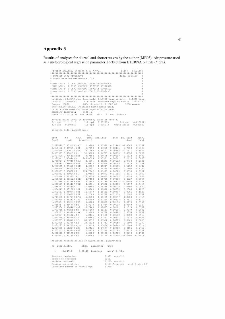
41
Appendix 3
Results of analyses for diurnal and shorter waves by the author (ME03). Air pressure used
as a meteorological regression parameter. Picked from ETERNA out file (*.prn). Program ANALYZE, version 3.40 970921 File: 9402icet #################################################################### # STATION 0892 METSÄHOVI Tidal gravity # # SUPERCONDUCTNG GRAVIMETER T020 # # # #TIME LAG : 0.0690 DEG/CPD 19941201-19970905 # #TIME LAG : 0.0395 DEG/CPD 19970905-19990315 # #TIME LAG : 0.0690 DEG/CPD 19990315-20010103 # #TIME LAG : 0.0395 DEG/CPD 20010103-20020901 # # # #################################################################### Latitude: 60.2172 deg, longitude: 24.3958 deg, azimuth: 0.0000 deg. 19941201...20020901 6 blocks. Recorded days in total: 2620.250 Tamura (1987) TGP, threshold: 0.100E-06 1200 waves. WAHR-DEHANT-ZSCHAU inelastic Earth model used. UNITY window used for least squares adjustment. Sampling interval: 3600. s Numerical filter is PERTZEV59 with 51 coefficients. Average noise level at frequency bands in nm/s**2 0.1 cpd*********** 1.0 cpd 0.031835 2.0 cpd 0.013862 3.0 cpd 0.007950 4.0 cpd 0.005573 white noise 0.006880 adjusted tidal parameters : theor. from to wave ampl. ampl.fac. stdv. ph. lead stdv. [cpd] [cpd] [nm/s**2 ] [deg] [deg] 0.721499 0.833113 SGQ1 1.9800 1.15529 0.01448 -1.0346 0.7182 0.851182 0.859691 2Q1 6.7910 1.14060 0.00435 -0.7903 0.2188 0.860896 0.870023 SGM1 8.1960 1.15173 0.00368 -0.1611 0.1829 0.887325 0.896130 Q1 51.3220 1.14709 0.00056 0.0057 0.0282 0.897806 0.906315 RO1 9.7484 1.14675 0.00299 -0.1132 0.1493 0.921941 0.930449 O1 268.0524 1.15321 0.00011 0.2618 0.0053 0.931964 0.940488 TAU1 3.4961 1.15241 0.00632 -0.0732 0.3145 0.958085 0.966756 NO1 21.0813 1.15949 0.00119 0.2338 0.0588 0.968565 0.974189 CHI1 4.0319 1.15817 0.00696 0.1259 0.3442 0.989048 0.995144 PI1 7.2941 1.15230 0.00348 0.1807 0.1732 0.996967 0.998028 P1 124.7242 1.15425 0.00020 0.0639 0.0101 0.999852 1.000148 S1 2.9495 1.14872 0.01215 7.4811 0.6059 1.001824 1.003651 K1 376.9855 1.14055 0.00007 0.0793 0.0036 1.005328 1.005623 PSI1 2.9494 1.25785 0.00868 0.4927 0.3954 1.007594 1.013689 PHI1 5.3682 1.17185 0.00472 -0.6954 0.2308 1.028549 1.034467 TET1 4.0311 1.17252 0.00700 0.1097 0.3418 1.036291 1.044800 J1 21.0805 1.15796 0.00129 0.0400 0.0640 1.064841 1.071083 SO1 3.4969 1.16098 0.00856 0.2389 0.4228 1.072583 1.080945 OO1 11.5349 1.15432 0.00307 0.0051 0.1523 1.099161 1.216397 NU1 2.2085 1.16790 0.01539 0.2680 0.7551 1.719380 1.837970 EPS2 1.3704 1.15185 0.00747 1.0880 0.3714 1.853920 1.862429 2N2 4.6999 1.17220 0.00227 1.3521 0.1110 1.863634 1.872142 MU2 5.6720 1.16855 0.00196 1.0099 0.0959 1.888387 1.896748 N2 35.5178 1.17864 0.00030 1.0389 0.0147 1.897954 1.906462 NU2 6.7463 1.18035 0.00161 1.1019 0.0782 1.923765 1.942754 M2 185.5103 1.18133 0.00006 0.7079 0.0028 1.958232 1.963709 LAM2 1.3680 1.16738 0.00782 0.5754 0.3839 1.965827 1.976926 L2 5.2435 1.17606 0.00188 0.3802 0.0918 1.991786 1.998288 T2 5.0462 1.17251 0.00221 0.1630 0.1078 1.999705 2.000766 S2 86.3092 1.17552 0.00013 0.0765 0.0063 2.002590 2.013689 K2 23.4632 1.17752 0.00055 0.1800 0.0270 2.031287 2.047390 ETA2 1.3119 1.17656 0.00968 -0.2109 0.4714 2.067579 2.182844 2K2 0.3436 1.17577 0.03790 -2.4586 1.8468 2.753243 2.869714 MN3 0.4974 1.07710 0.01190 0.6315 0.6328 2.892640 3.081254 M3 1.8128 1.08188 0.00329 0.3410 0.1744 3.791963 3.901458 M4 0.0164 0.41165 0.24206 158.6900 33.6911 Adjusted meteorological or hydrological parameters: no. regr.coeff. stdv. parameter unit 1 -3.64710 0.00443 Airpress nm/s**2 /hPa Standard deviation: 0.971 nm/s**2 Degree of freedom: 62513 Maximum residual: 15.275 nm/s**2 Maximum correlation: 0.101 Airpress with X-wave-S2 Condition number of normal equ. 1.539

42

43
Publications