Embed Size (px)
Citation preview
STUDENT
SOLUTIONS MANUAL
to accompany
LINEAR ALGEBRA
Concepts and Applications
P. Bogacki
COURSE PACK for MATH 316
Fall 2015 Edition

This solutions manual has been prepared solely for the designated sections of Introductory Linear Algebra, MATH 316 taught at Old Dominion University.
Any other use requires an explicit permission from the author.
Copyright (c) 2004-2015 by P. Bogacki
(V.58a - 8/16/2015)
Student Solutions Manual 3
Section
1.1 1.−−→P1P2 =
[−1− 2
3− 5
]=
[−3
−2
];∥∥∥−−→P1P2
∥∥∥ =√(−3)2 + (−2)2 =√13.
3.−−−→Q2Q1 =
⎡⎢⎣ 0− 2
−2− 2
1− 1
⎤⎥⎦ =
⎡⎢⎣ −2
−4
0
⎤⎥⎦ ;∥∥∥−−−→Q2Q1
∥∥∥ =√(−2)2 + (−4)2 + 02 =√20 = 2
√5
5. a. −→u +−→w =
[1
2
]+
[0
3
]=
[1
5
]
b. 2−→v = 2
[6
−4
]=
[12
−8
]
c. −−→w = −[
0
3
]=
[0
−3
]d. ‖−→w ‖ =
√02 +32 = 3
7. 2−→u −−→v = 2
[1
2
]−[
6
−4
]=
[−4
8
]
9. − (3−→u +−→v ) +−→w = −(3
[1
2
]+
[6
−4
]) +
[0
3
]=
[−9
1
]
11. −→u · −→v = (1)(6) + (2)(−4) = −2.
13. −→w · −→w = (0)(0) + (3)(3) = 9.
15. a. −→u +−→w =
⎡⎢⎣ −1
0
2
⎤⎥⎦+
⎡⎢⎣ 0
2
2
⎤⎥⎦ =
⎡⎢⎣ −1
2
4
⎤⎥⎦
b. 2−→v = 2
⎡⎢⎣ 1
2
−3
⎤⎥⎦ =
⎡⎢⎣ 2
4
−6
⎤⎥⎦
c. −−→w = −
⎡⎢⎣ 0
2
2
⎤⎥⎦ =
⎡⎢⎣ 0
−2
−2
⎤⎥⎦d. ‖−→w ‖ =
√02 +22 +22 =
√8 = 2
√2
17. −→w + 4−→v =
⎡⎢⎣ 0
2
2
⎤⎥⎦+4
⎡⎢⎣ 1
2
−3
⎤⎥⎦ =
⎡⎢⎣ 4
10
−10
⎤⎥⎦
19. 4−→u − (−→v −−→w ) = 4
⎡⎢⎣ −1
0
2
⎤⎥⎦− (
⎡⎢⎣ 1
2
−3
⎤⎥⎦−
⎡⎢⎣ 0
2
2
⎤⎥⎦) = 4
⎡⎢⎣ −1
0
2
⎤⎥⎦−
⎡⎢⎣ 1
0
−5
⎤⎥⎦ =
⎡⎢⎣ −5
0
13
⎤⎥⎦
4 Student Solutions Manual
21. 1‖−→w ‖
−→w = 1√0+4+4
⎡⎢⎣ 0
2
2
⎤⎥⎦ = 12√2
⎡⎢⎣ 0
2
2
⎤⎥⎦ =
⎡⎢⎢⎣01√21√2
⎤⎥⎥⎦23. −→u · −→w = (−1)(0) + (0)(2) + (2)(2) = 4
25. a. −→u +−→w =
⎡⎢⎢⎢⎢⎣2
1
0
2
⎤⎥⎥⎥⎥⎦+
⎡⎢⎢⎢⎢⎣2
0
3
0
⎤⎥⎥⎥⎥⎦ =
⎡⎢⎢⎢⎢⎣4
1
3
2
⎤⎥⎥⎥⎥⎦
b. 2−→v = 2
⎡⎢⎢⎢⎢⎣−1
3
1
2
⎤⎥⎥⎥⎥⎦ =
⎡⎢⎢⎢⎢⎣−2
6
2
4
⎤⎥⎥⎥⎥⎦
c. −−→w = −
⎡⎢⎢⎢⎢⎣2
0
3
0
⎤⎥⎥⎥⎥⎦ =
⎡⎢⎢⎢⎢⎣−2
0
−3
0
⎤⎥⎥⎥⎥⎦d. ‖−→w ‖ =
√22 +02 +32 +02 =
√13
27. −2−→u +−→w = −2
⎡⎢⎢⎢⎢⎣2
1
0
2
⎤⎥⎥⎥⎥⎦+
⎡⎢⎢⎢⎢⎣2
0
3
0
⎤⎥⎥⎥⎥⎦ =
⎡⎢⎢⎢⎢⎣−2
−2
3
−4
⎤⎥⎥⎥⎥⎦29. −→v · −→v = (−1)(−1) + (3)(3) + (1)(1) + (2)(2) = 15
31. TRUE
Since ‖−→u ‖ =√a21 + a22 + · · ·+ a2n, all components of −→u (a1, a2, . . . , an) must be zero for the sum of
their squares to be zero. (In other words, the only vector with zero length is the zero vector.)
33. FALSE⎡⎢⎣ 1
2
−3
⎤⎥⎦ ·
⎡⎢⎣ 3
0
−1
⎤⎥⎦ = (1)(3) + (2)(0) + (−3)(−1) = 6 �= 0.
35. True for all vectors and scalars
c(−→u −−→v ) = c(−→u + (−1)−→v )
= c−→u + c((−1)−→v ) by Property 7 of Theorem 1.1
= c−→u + (−c−→v ) by Property 9 of Theorem 1.1
= c−→u − c−→v
37. Counterexample: −→u =
⎡⎢⎣ 1
0
0
⎤⎥⎦ , c = −3.
LHS =
∥∥∥∥∥∥∥⎡⎢⎣ −3
0
0
⎤⎥⎦∥∥∥∥∥∥∥ = 3
Student Solutions Manual 5
RHS = −3
∥∥∥∥∥∥∥⎡⎢⎣ 1
0
0
⎤⎥⎦∥∥∥∥∥∥∥ = −3
LHS �= RHS
39. Counterexample: −→u =
[3
0
],−→v =
[2
0
],−→w =
[1
0
]
LHS =
[1
0
]−[
1
0
]=
[0
0
]
RHS =
[3
0
]−[
1
0
]=
[2
0
]
LHSgenerally
�= = RHS
45. a.
⎡⎢⎣ 1
1
3
⎤⎥⎦×
⎡⎢⎣ 2
1
0
⎤⎥⎦ =
⎡⎢⎣ (1)(0) − (3)(1)
(3)(2) − (1)(0)
(1)(1) − (1)(2)
⎤⎥⎦ =
⎡⎢⎣ −3
6
−1
⎤⎥⎦
b.
⎡⎢⎣ 3
−1
2
⎤⎥⎦×
⎡⎢⎣ −6
2
−4
⎤⎥⎦ =
⎡⎢⎣ (−1)(−4)− (2)(2)
(2)(−6)− (3)(−4)
(3)(2)− (−1)(−6)
⎤⎥⎦ =
⎡⎢⎣ 0
0
0
⎤⎥⎦51. a. −→p =
[1
4
]; −→q =
[2
2
]; −→p +−→q =
[3
6
];
b. −→u =
[3
3
]; −→v =
[4
1
]; −→u +−→v =
[7
4
]y
A
CD
B
1
1
y'
x
x'
53. −→a = 0.40−→t +0.25−→q + 0.35−→f
6 Student Solutions Manual
Section
1.21. a. a21 = −2,
b. a34 = −4,
c. col3A =
⎡⎢⎣ 0
−3
−5
⎤⎥⎦ ,d. row2A =
[−2 3 −3 1
],
e. AT =
⎡⎢⎢⎢⎢⎣2 −2 4
1 3 5
0 −3 −5
−1 1 −4
⎤⎥⎥⎥⎥⎦ .
3.
Matrix in Exercise # K L M N
a. a diagonal matrix Yes Yes No No
b. an upper triangular matrix Yes Yes No No
c. a lower tiangular matrix Yes Yes Yes No
d. a scalar matrix No Yes No No
e. an identity matrix No No No No
f. a symmetric matrix Yes Yes No No
5. a.
⎡⎢⎣ 3 0
5 −2
2 0
⎤⎥⎦+
⎡⎢⎣ 1 −1
3 0
−2 3
⎤⎥⎦ =
⎡⎢⎣ 4 −1
8 −2
0 3
⎤⎥⎦b.
[10 5
−1 0
]+
[1 0 0
3 1 0
]cannot be evaluated
c. −3
⎡⎢⎣ 6 1
1 1
0 0
⎤⎥⎦ =
⎡⎢⎣ −18 −3
−3 −3
0 0
⎤⎥⎦
7. LHS =
[3 −1
1 2
]+
[1 3
0 4
]=
[4 2
1 6
]
RHS =
[1 3
0 4
]+
[3 −1
1 2
]=
[4 2
1 6
]
9.(AT)T
=
[3 1
−1 2
]T=
[3 −1
1 2
]= A
11. A =
⎡⎢⎣ 0 0 3
0 0 −1
−3 1 0
⎤⎥⎦ is skew-symmetric, since AT =
⎡⎢⎣ 0 0 −3
0 0 1
3 −1 0
⎤⎥⎦ = −A.
B =
[1 3
−3 −1
]is not skew-symmetric, since BT =
[1 −3
3 −1
]�=[
−1 −3
3 1
]= −B
Student Solutions Manual 7
C =
⎡⎢⎣ 0 −4
4 0
0 0
⎤⎥⎦ is not skew-symmetric, since CT =
[0 4 0
−4 0 0
]�=
⎡⎢⎣ 0 4
−4 0
0 0
⎤⎥⎦ = −C
D =
[0 0
0 0
]is skew-symmetric since DT =
[0 0
0 0
]= −D.
13. A =
⎡⎢⎢⎢⎢⎣1 3 0 0
2 −1 5 0
0 4 1 7
0 0 6 −1
⎤⎥⎥⎥⎥⎦ is tridiagonal since the entries where i > j + 1 or i < j − 1 (in boxes)
are all 0;
B =
⎡⎢⎢⎢⎢⎢⎢⎣0 1 0 0 0
0 0 0 0 0
0 1 0 1 0
0 0 0 0 0
0 0 0 1 0
⎤⎥⎥⎥⎥⎥⎥⎦ is tridiagonal since the entries where i > j + 1 or i < j − 1 (in
boxes) are all 0;
C =
⎡⎢⎣ 1 0 1
0 1 0
0 0 1
⎤⎥⎦ is not tridiagonal because c13 = 1 �= 0.
15. TRUE
3A︸︷︷︸2×3
+ 4B︸︷︷︸2×3︸ ︷︷ ︸
2×3
17. TRUE
by Property 2 of Theorem 1.4
19. FALSE
AT︸︷︷︸4×3
+ A︸︷︷︸3×4︸ ︷︷ ︸
cannot evaluate
21. TRUE
If m �= n then anm× n matrix A and the n×m matrix AT cannot possibly be equal.
23. Example:
[2 0
0 2
]
25. Example:
⎡⎢⎣ 0 0 0
0 0 0
0 0 0
⎤⎥⎦
8 Student Solutions Manual
Section
1.3 1. a. CD =
[3 4
5 −2
][4 1 1
1 −1 −1
]=
[16 −1 −1
18 7 7
]b. DC cannot be evaluated (the number of columns inD does not match the number of rows inC).
c. AD =
⎡⎢⎣ 2 −1
3 0
2 1
⎤⎥⎦[ 4 1 1
1 −1 −1
]=
⎡⎢⎣ 7 3 3
12 3 3
9 1 1
⎤⎥⎦
d. DA =
[4 1 1
1 −1 −1
] ⎡⎢⎣ 2 −1
3 0
2 1
⎤⎥⎦ =
[13 −3
−3 −2
]
e. CE =
[3 4
5 −2
][2 0
0 2
]=
[6 8
10 −4
]
f. EC =
[2 0
0 2
][3 4
5 −2
]=
[6 8
10 −4
]
3. a. (AC)T =
⎛⎜⎝⎡⎢⎣ 2 −1
3 0
2 1
⎤⎥⎦[ 3 4
5 −2
]⎞⎟⎠T
=
⎡⎢⎣ 1 10
9 12
11 6
⎤⎥⎦T
=
[1 9 11
10 12 6
]
b. ATCT cannot be evaluated(the number of columns inAT does not match the number of rows inCT ).
c. CTAT =
[3 5
4 −2
][2 3 2
−1 0 1
]=
[1 9 11
10 12 6
]
d.(BTC
)T=
⎛⎜⎜⎜⎜⎝⎡⎢⎢⎢⎢⎣
4 2
0 −2
0 0
1 3
⎤⎥⎥⎥⎥⎦[
3 4
5 −2
]⎞⎟⎟⎟⎟⎠T
=
⎡⎢⎢⎢⎢⎣22 12
−10 4
0 0
18 −2
⎤⎥⎥⎥⎥⎦T
=
[22 −10 0 18
12 4 0 −2
]
e. CTB =
[3 5
4 −2
][4 0 0 1
2 −2 0 3
]=
[22 −10 0 18
12 4 0 −2
]
5. a. C2 = CC =
[3 4
5 −2
][3 4
5 −2
]=
[29 4
5 24
]b. D2 = DD cannot be evaluated(D is not a square matrix).
7. a. ED+CAT =
[2 0
0 2
][4 1 1
1 −1 −1
]+
[3 4
5 −2
][2 3 2
−1 0 1
]
=
[8 2 2
2 −2 −2
]+
[2 9 10
12 15 8
]=
[10 11 12
14 13 6
]
b.(AC)D =
⎛⎜⎝⎡⎢⎣ 2 −1
3 0
2 1
⎤⎥⎦[ 3 4
5 −2
]⎞⎟⎠[ 4 1 1
1 −1 −1
]
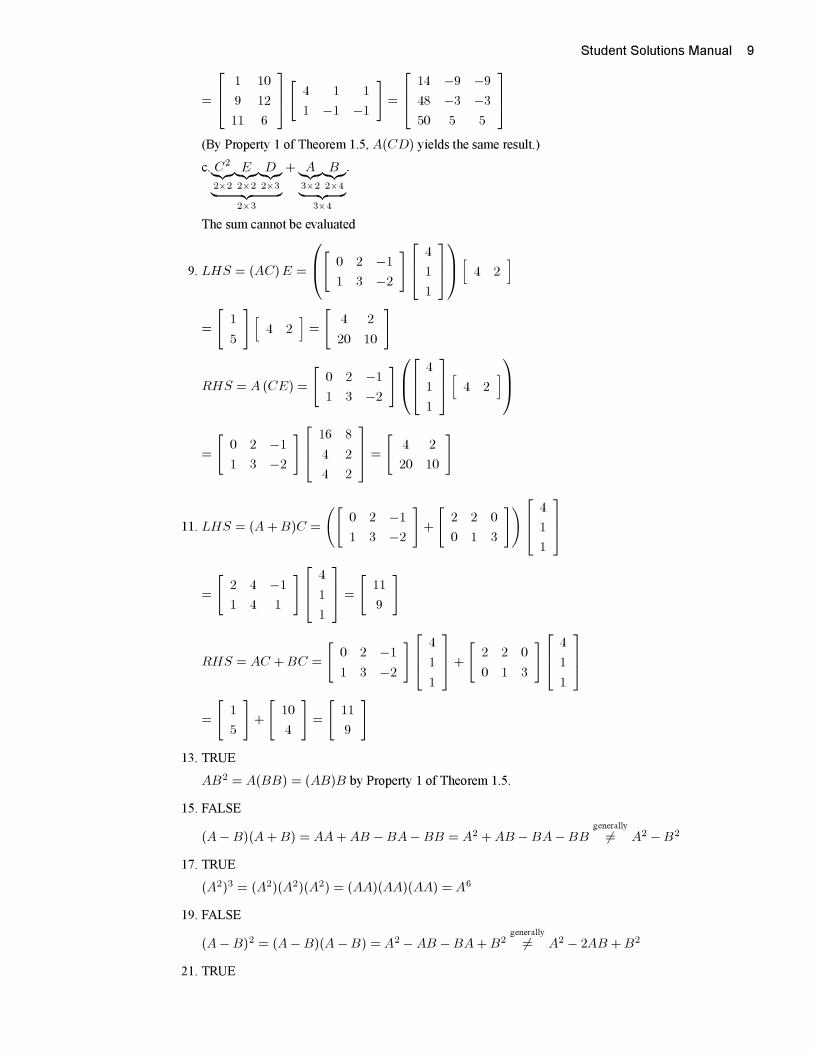
Student Solutions Manual 9
=
⎡⎢⎣ 1 10
9 12
11 6
⎤⎥⎦[ 4 1 1
1 −1 −1
]=
⎡⎢⎣ 14 −9 −9
48 −3 −3
50 5 5
⎤⎥⎦(By Property 1 of Theorem 1.5, A(CD) yields the same result.)
c. C2︸︷︷︸2×2
E︸︷︷︸2×2
D︸︷︷︸2×3︸ ︷︷ ︸
2×3
+ A︸︷︷︸3×2
B︸︷︷︸2×4︸ ︷︷ ︸
3×4
.
The sum cannot be evaluated
9. LHS = (AC)E =
⎛⎜⎝[ 0 2 −1
1 3 −2
]⎡⎢⎣ 4
1
1
⎤⎥⎦⎞⎟⎠[ 4 2
]
=
[1
5
] [4 2
]=
[4 2
20 10
]
RHS = A (CE) =
[0 2 −1
1 3 −2
]⎛⎜⎝⎡⎢⎣ 4
1
1
⎤⎥⎦[ 4 2]⎞⎟⎠
=
[0 2 −1
1 3 −2
]⎡⎢⎣ 16 8
4 2
4 2
⎤⎥⎦ =
[4 2
20 10
]
11. LHS = (A+B)C =
([0 2 −1
1 3 −2
]+
[2 2 0
0 1 3
])⎡⎢⎣ 4
1
1
⎤⎥⎦
=
[2 4 −1
1 4 1
]⎡⎢⎣ 4
1
1
⎤⎥⎦ =
[11
9
]
RHS = AC +BC =
[0 2 −1
1 3 −2
]⎡⎢⎣ 4
1
1
⎤⎥⎦+
[2 2 0
0 1 3
]⎡⎢⎣ 4
1
1
⎤⎥⎦=
[1
5
]+
[10
4
]=
[11
9
]13. TRUE
AB2 = A(BB) = (AB)B by Property 1 of Theorem 1.5.
15. FALSE
(A−B)(A+B) = AA+AB −BA−BB = A2 +AB −BA−BBgenerally
�= A2 −B2
17. TRUE
(A2)3 = (A2)(A2)(A2) = (AA)(AA)(AA) = A6
19. FALSE
(A−B)2 = (A−B)(A−B) = A2 −AB −BA+B2generally
�= A2 − 2AB +B2
21. TRUE
10 Student Solutions Manual
(ATB)T = BT (AT )T = BTA
follows from Property 5 of Theorem 1.5 and Property 3 of Theorem 1.4.
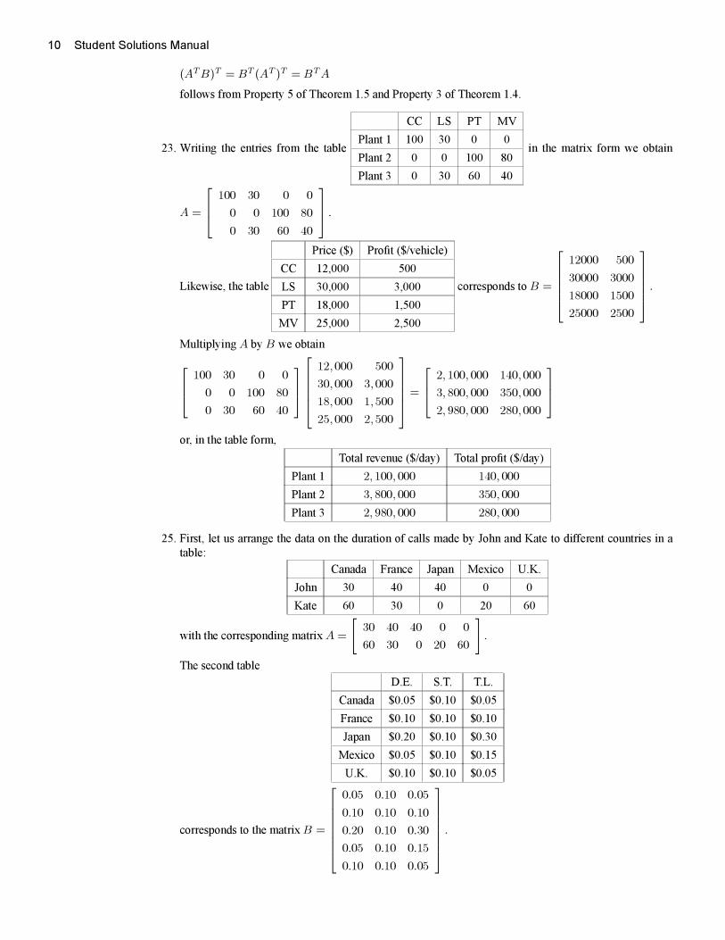
23. Writing the entries from the table
CC LS PT MV
Plant 1 100 30 0 0
Plant 2 0 0 100 80
Plant 3 0 30 60 40
in the matrix form we obtain
A =
⎡⎢⎣ 100 30 0 0
0 0 100 80
0 30 60 40
⎤⎥⎦ .
Likewise, the table
Price ($) Profit ($/vehicle)
CC 12,000 500
LS 30,000 3,000
PT 18,000 1,500
MV 25,000 2,500
corresponds to B =
⎡⎢⎢⎢⎢⎣12000 500
30000 3000
18000 1500
25000 2500
⎤⎥⎥⎥⎥⎦ .
Multiplying A by B we obtain⎡⎢⎣ 100 30 0 0
0 0 100 80
0 30 60 40
⎤⎥⎦⎡⎢⎢⎢⎢⎣
12,000 500
30,000 3,000
18,000 1,500
25,000 2,500
⎤⎥⎥⎥⎥⎦ =
⎡⎢⎣ 2, 100, 000 140,000
3, 800, 000 350,000
2, 980, 000 280,000
⎤⎥⎦or, in the table form,
Total revenue ($/day) Total profit ($/day)
Plant 1 2, 100, 000 140, 000
Plant 2 3, 800, 000 350, 000
Plant 3 2, 980, 000 280, 000
25. First, let us arrange the data on the duration of calls made by John and Kate to different countries in a
table:
Canada France Japan Mexico U.K.
John 30 40 40 0 0
Kate 60 30 0 20 60
with the corresponding matrix A =
[30 40 40 0 0
60 30 0 20 60
].
The second table
D.E. S.T. T.L.
Canada $0.05 $0.10 $0.05
France $0.10 $0.10 $0.10
Japan $0.20 $0.10 $0.30
Mexico $0.05 $0.10 $0.15
U.K. $0.10 $0.10 $0.05
corresponds to the matrix B =
⎡⎢⎢⎢⎢⎢⎢⎣0.05 0.10 0.05
0.10 0.10 0.10
0.20 0.10 0.30
0.05 0.10 0.15
0.10 0.10 0.05
⎤⎥⎥⎥⎥⎥⎥⎦ .
Student Solutions Manual 11
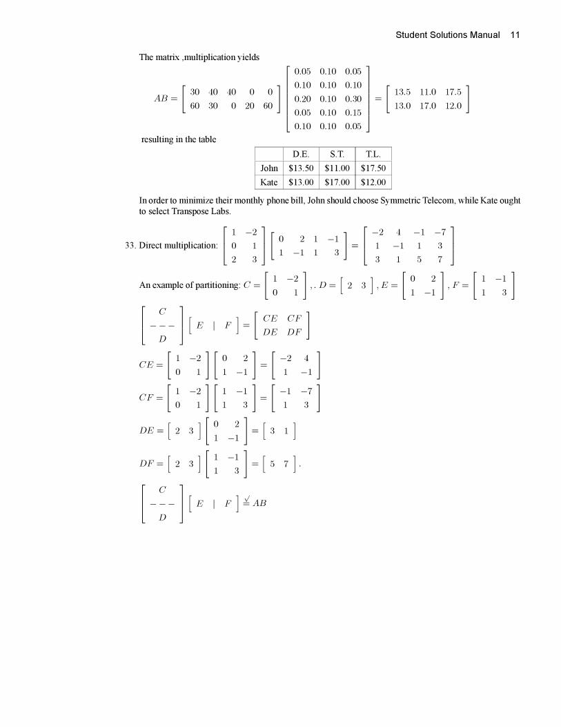
The matrix ,multiplication yields
AB =
[30 40 40 0 0
60 30 0 20 60
]⎡⎢⎢⎢⎢⎢⎢⎣
0.05 0.10 0.05
0.10 0.10 0.10
0.20 0.10 0.30
0.05 0.10 0.15
0.10 0.10 0.05
⎤⎥⎥⎥⎥⎥⎥⎦ =
[13.5 11.0 17.5
13.0 17.0 12.0
]
resulting in the table
D.E. S.T. T.L.
John $13.50 $11.00 $17.50
Kate $13.00 $17.00 $12.00
In order to minimize their monthly phone bill, John should choose Symmetric Telecom, while Kate ought
to select Transpose Labs.
33. Direct multiplication:
⎡⎢⎣ 1 −2
0 1
2 3
⎤⎥⎦[ 0 2 1 −1
1 −1 1 3
]=
⎡⎢⎣ −2 4 −1 −7
1 −1 1 3
3 1 5 7
⎤⎥⎦An example of partitioning: C =
[1 −2
0 1
], . D =
[2 3
], E =
[0 2
1 −1
], F =
[1 −1
1 3
]⎡⎢⎣ C
−−−D
⎤⎥⎦[ E | F]=
[CE CF
DE DF
]
CE =
[1 −2
0 1
][0 2
1 −1
]=
[−2 4
1 −1
]
CF =
[1 −2
0 1
] [1 −1
1 3
]=
[−1 −7
1 3
]
DE =[2 3
][ 0 2
1 −1
]=[3 1
]
DF =[2 3
] [ 1 −1
1 3
]=[5 7
].
⎡⎢⎣ C
−−−D
⎤⎥⎦[ E | F] √= AB
12 Student Solutions Manual
Section
1.4 1. The matrix is
[1 1
2
0 1
]. F (
[3
2
]) =
[1 1
2
0 1
][3
2
]=
[4
2
].
3. From F (
[1
0
]) =
[2
0
]and F (
[0
1
]) =
[0
−1
]we obtain the matrix
[2 0
0 −1
].
5. From F (
[1
0
]) =
[0
0
]and F (
[0
1
]) =
[0
1
]we obtain the matrix
[0 0
0 1
].
7. x1
[2
3
]+ x2
[−1
0
]=
[2 −1
3 0
][x1
x2
]; The matrix is
[2 −1
3 0
].
9. 2x1
⎡⎢⎣ −2
8
1
⎤⎥⎦− x3
⎡⎢⎣ 4
0
0
⎤⎥⎦ = x1
⎡⎢⎣ −4
16
2
⎤⎥⎦+ x2
⎡⎢⎣ 0
0
0
⎤⎥⎦+ x3
⎡⎢⎣ −4
0
0
⎤⎥⎦ =
⎡⎢⎣ −4 0 −4
16 0 0
2 0 0
⎤⎥⎦⎡⎢⎣ x1
x2
x3
⎤⎥⎦ .
The matrix is
⎡⎢⎣ −4 0 −4
16 0 0
2 0 0
⎤⎥⎦ .
11. x1
[6
1
]+ 3x2
[3
2
]+ x4
[−2
7
]= x1
[6
1
]+ x2
[9
6
]+ x3
[0
0
]+ x4
[−2
7
]
=
[6 9 0 −2
1 6 0 7
]⎡⎢⎢⎢⎢⎣x1
x2
x3
x4
⎤⎥⎥⎥⎥⎦ ; The matrix is
[6 9 0 −2
1 6 0 7
]
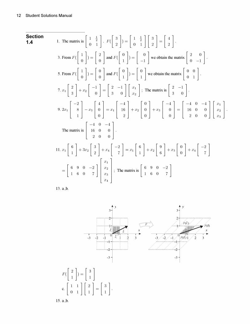
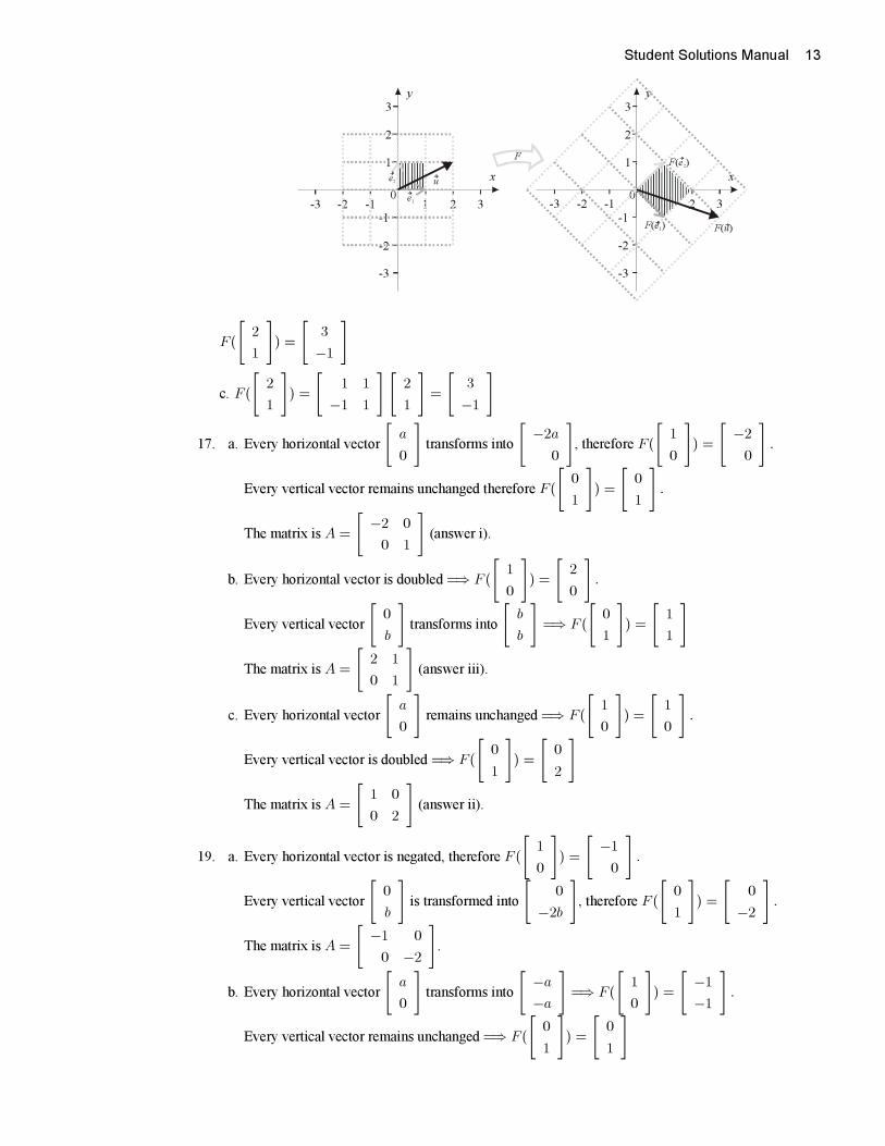
13. a.,b.
x
1 1
1 1
-1 -1
-1 -1
-2 -2
-2 -2
-3 -3
-3 -3
2 2
2 2
3 3
3 3
0 0
x
y y
F
e2
e1
u
F e( )2
F e( )1
F u( )
F (
[2
1
]) =
[3
1
]
c.
[1 1
0 1
][2
1
]=
[3
1
].
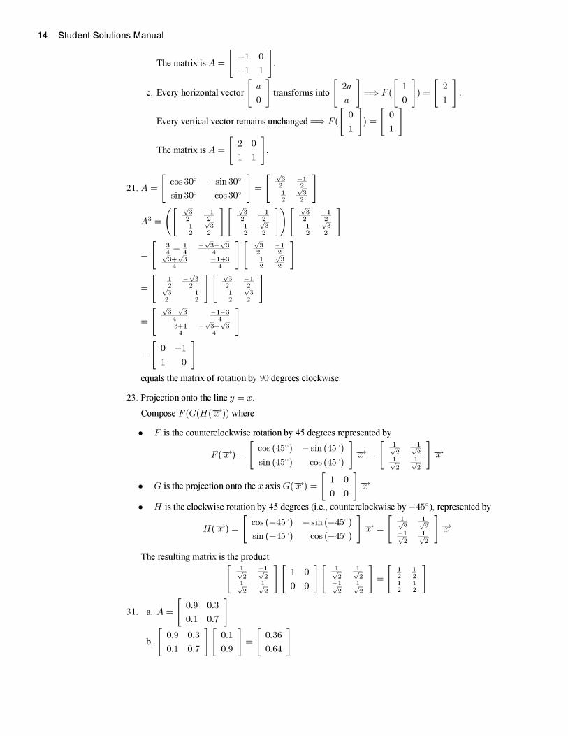
15. a.,b.
Student Solutions Manual 13
x
1 1
1 1
-1 -1
-1 -1
-2 -2
-2 -2
-3 -3
-3 -3
2 2
2 2
3 3
3 3
0 0
x
y y
F
e2
e1
u
F e( )2
F e( )1 F u( )
F (
[2
1
]) =
[3
−1
]
c. F (
[2
1
]) =
[1 1
−1 1
] [2
1
]=
[3
−1
]
17. a. Every horizontal vector
[a
0
]transforms into
[−2a
0
], therefore F (
[1
0
]) =
[−2
0
].
Every vertical vector remains unchanged therefore F (
[0
1
]) =
[0
1
].
The matrix is A =
[−2 0
0 1
](answer i).
b. Every horizontal vector is doubled=⇒ F (
[1
0
]) =
[2
0
].
Every vertical vector
[0
b
]transforms into
[b
b
]=⇒ F (
[0
1
]) =
[1
1
]
The matrix is A =
[2 1
0 1
](answer iii).
c. Every horizontal vector
[a
0
]remains unchanged=⇒ F (
[1
0
]) =
[1
0
].
Every vertical vector is doubled =⇒ F (
[0
1
]) =
[0
2
]
The matrix is A =
[1 0
0 2
](answer ii).
19. a. Every horizontal vector is negated, therefore F (
[1
0
]) =
[−1
0
].
Every vertical vector
[0
b
]is transformed into
[0
−2b
], therefore F (
[0
1
]) =
[0
−2
].
The matrix is A =
[−1 0
0 −2
].
b. Every horizontal vector
[a
0
]transforms into
[−a
−a
]=⇒ F (
[1
0
]) =
[−1
−1
].
Every vertical vector remains unchanged=⇒ F (
[0
1
]) =
[0
1
]
14 Student Solutions Manual
The matrix is A =
[−1 0
−1 1
].
c. Every horizontal vector
[a
0
]transforms into
[2a
a
]=⇒ F (
[1
0
]) =
[2
1
].
Every vertical vector remains unchanged=⇒ F (
[0
1
]) =
[0
1
]
The matrix is A =
[2 0
1 1
].
21. A =
[cos 30◦ − sin 30◦
sin 30◦ cos 30◦
]=
[ √32
−12
12
√32
]
A3 =
([ √32
−12
12
√32
][ √32
−12
12
√32
])[ √32
−12
12
√32
]
=
[34 − 1
4−√
3−√3
4√3+
√3
4−1+3
4
][ √32
−12
12
√32
]
=
[12
−√3
2√32
12
] [ √32
−12
12
√32
]
=
[ √3−√
34
−1−34
3+14
−√3+
√3
4
]
=
[0 −1
1 0
]equals the matrix of rotation by 90 degrees clockwise.
23. Projection onto the line y = x.
Compose F (G(H(−→x )) where
• F is the counterclockwise rotation by 45 degrees represented by
F (−→x ) =
[cos (45◦) − sin (45◦)
sin (45◦) cos (45◦)
]−→x =
[1√2
−1√2
1√2
1√2
]−→x
• G is the projection onto the x axis G(−→x ) =
[1 0
0 0
]−→x
• H is the clockwise rotation by 45 degrees (i.e., counterclockwise by −45◦), represented by
H(−→x ) =
[cos (−45◦) − sin (−45◦)sin (−45◦) cos (−45◦)
]−→x =
[1√2
1√2
−1√2
1√2
]−→x
The resulting matrix is the product[1√2
−1√2
1√2
1√2
][1 0
0 0
][1√2
1√2
−1√2
1√2
]=
[12
12
12
12
]
31. a. A =
[0.9 0.3
0.1 0.7
]
b.
[0.9 0.3
0.1 0.7
][0.1
0.9
]=
[0.36
0.64
]
Student Solutions Manual 15
Section
2.1 1. Augmented matrix
[1 6 | 0
0 3 | 1
]; Coefficient matrix
[1 6
0 3
]
3. Augmented matrix
⎡⎢⎢⎢⎢⎣0 0 1 | 4
7 0 3 | 5
0 5 0 | −6
1 −1 0 | 3
⎤⎥⎥⎥⎥⎦; Coefficient matrix
⎡⎢⎢⎢⎢⎣0 0 1
7 0 3
0 5 0
1 −1 0
⎤⎥⎥⎥⎥⎦5. a.
2x − 3y = 4
6x = 0
b.
x + 2y + z = 2
3x − z = 0
y + z = 0
0 = 1
7. a. (i) both reduced row echelon form, and row echelon form
b. (ii) row echelon form, but not in reduced row echelon form
c. (iii) neither (zero row above nonzero row)
d. (iii) neither (rows 2 and 3 do not follow the staircase pattern)
9. a. i.
[1 0 | 0
0 1 | 2
].
ii. one solution
iii. x = 0, y = 2
b. i.
⎡⎢⎣ 1 0 | 0
0 1 | 0
0 0 | 1
⎤⎥⎦ .ii. no solution
c. i.
[1 0 −3 | 4
0 1 2 | 5
].
ii. infinitely many solutions
iii. x = 3z +4, y = −2z + 5, z−arbitrary
11. a. i.
⎡⎢⎢⎢⎢⎣1 3 0 | 0
0 0 1 | 0
0 0 0 | 1
0 0 0 | 0
⎤⎥⎥⎥⎥⎦ .ii. no solution
b. i.
⎡⎢⎣ 0 1 0 −5 0 | 0
0 0 1 3 0 | 0
0 0 0 0 1 | 0
⎤⎥⎦ .ii. infinitely many solutions
16 Student Solutions Manual
iii.
x1 = arbitrary
x2 = 5x4
x3 = −3x4
x4 = arbitrary
x5 = 0
13. a.
[1 5 | −2
5 2 | 13
]
b. r.e.f.:
[1 5 | −2
0 1 | −1
]; r.r.e.f.
[1 0 | 3
0 1 | −1
]c.
y = −1
x = −5y − 2 = 3
d. x = 3, y = −1.
e.3 + 5(−1)
�= −2
5(3) + 2(−1)�= 13
15. a. augmented matrix:
[2 4 | 3
1 2 | −1
]
b. r.e.f.:
[1 2 | 3
2
0 0 | 1
]; r.r.e.f.:
[1 2 | 0
0 0 | 1
]c.0 = 1⇒ No solution
d.0 = 1⇒ No solution
17. a. augmented matrix:
[2 1 3 −1 | 7
−1 3 2 4 | 0
]
b. r.e.f.:
[1 1
232
−12
| 72
0 1 1 1 | 1
]; r.r.e.f.:
[1 0 1 −1 | 3
0 1 1 1 | 1
]c.
x2 = −x3 − x4 +1
x1 =−1
2(−x3 − x4 +1)− 3
2x3 +
1
2x4 +
7
2
=1
2x3 +
1
2x4 − 1
2− 3
2x3 +
1
2x4 +
7
2= −x3 + x4 +3
x3 = arbitrary
x4 = arbitrary
d.
x1 = −x3 + x4 + 3
x2 = −x3 − x4 + 1
x3 = arbitrary
x4 = arbitrary
Student Solutions Manual 17
e.
2 (−x3 + x4 + 3) + (−x3 − x4 +1) + 3x3 − x4�= 7
− (−x3 + x4 + 3) + 3 (−x3 − x4 +1) + 2x3 + 4x4�= 0
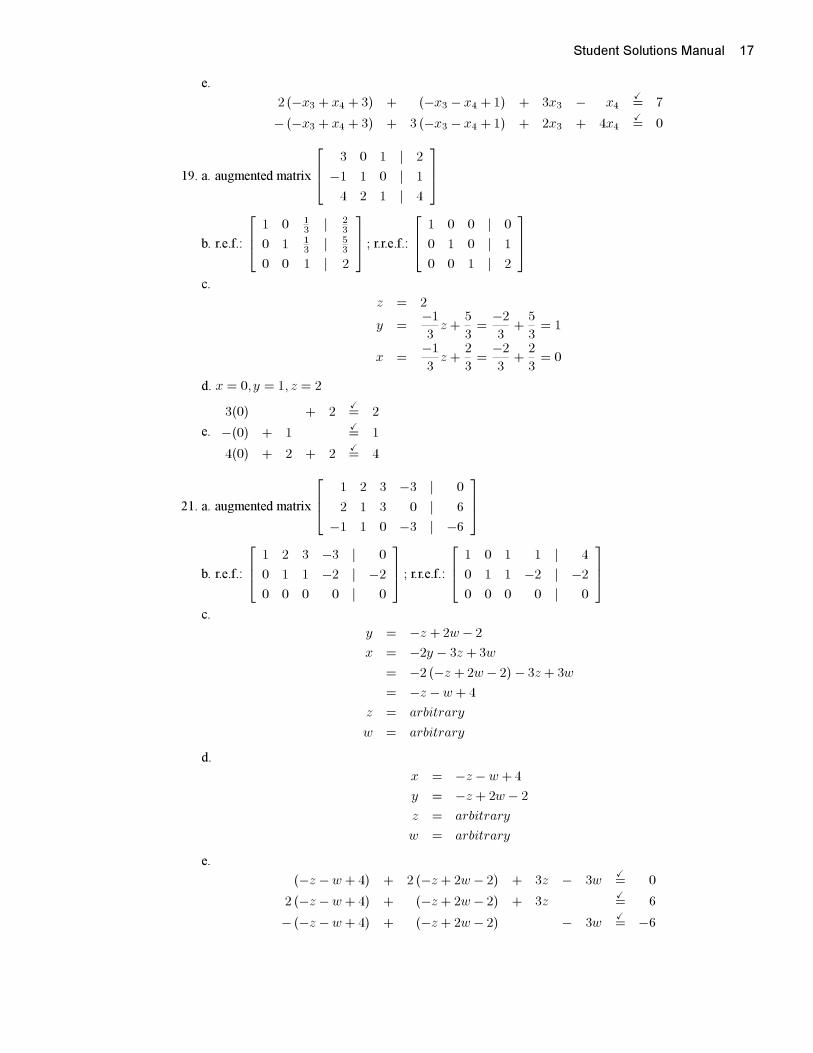
19. a. augmented matrix
⎡⎢⎣ 3 0 1 | 2
−1 1 0 | 1
4 2 1 | 4
⎤⎥⎦
b. r.e.f.:
⎡⎢⎣ 1 0 13 | 2
3
0 1 13 | 5
3
0 0 1 | 2
⎤⎥⎦ ; r.r.e.f.:⎡⎢⎣ 1 0 0 | 0
0 1 0 | 1
0 0 1 | 2
⎤⎥⎦c.
z = 2
y =−1
3z +
5
3=
−2
3+
5
3= 1
x =−1
3z +
2
3=
−2
3+
2
3= 0
d. x = 0, y = 1, z = 2
e.
3(0) + 2�= 2
−(0) + 1�= 1
4(0) + 2 + 2�= 4
21. a. augmented matrix
⎡⎢⎣ 1 2 3 −3 | 0
2 1 3 0 | 6
−1 1 0 −3 | −6
⎤⎥⎦
b. r.e.f.:
⎡⎢⎣ 1 2 3 −3 | 0
0 1 1 −2 | −2
0 0 0 0 | 0
⎤⎥⎦ ; r.r.e.f.:⎡⎢⎣ 1 0 1 1 | 4
0 1 1 −2 | −2
0 0 0 0 | 0
⎤⎥⎦c.
y = −z +2w − 2
x = −2y − 3z +3w
= −2 (−z +2w − 2) − 3z + 3w
= −z −w + 4
z = arbitrary
w = arbitrary
d.
x = −z −w +4
y = −z + 2w − 2
z = arbitrary
w = arbitrary
e.
(−z −w + 4) + 2 (−z + 2w − 2) + 3z − 3w�= 0
2 (−z −w + 4) + (−z + 2w − 2) + 3z�= 6
− (−z −w + 4) + (−z + 2w − 2) − 3w�= −6
18 Student Solutions Manual
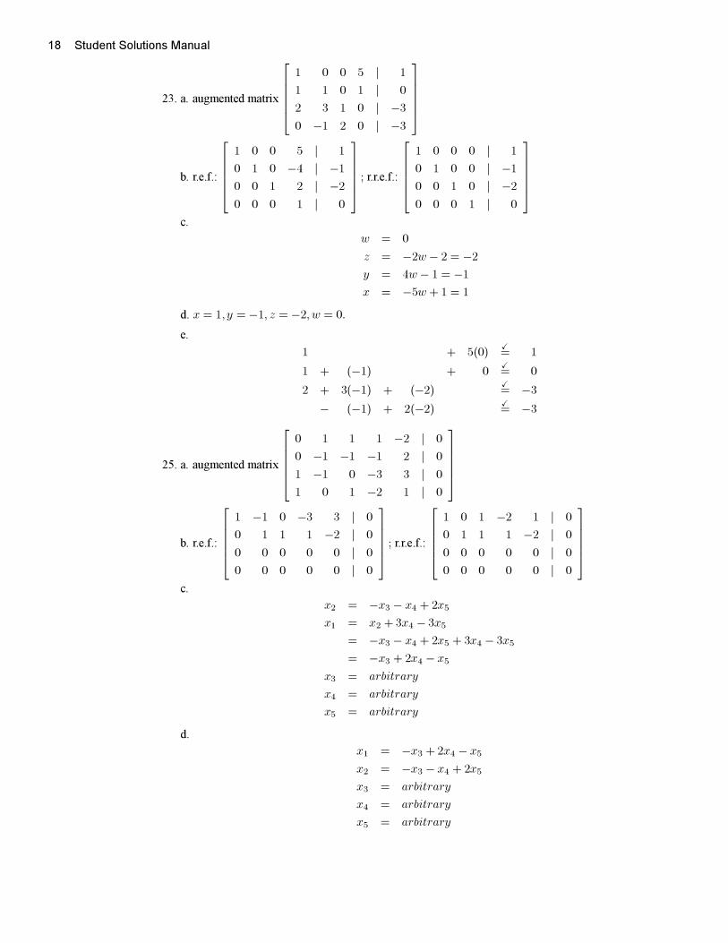
23. a. augmented matrix
⎡⎢⎢⎢⎢⎣1 0 0 5 | 1
1 1 0 1 | 0
2 3 1 0 | −3
0 −1 2 0 | −3
⎤⎥⎥⎥⎥⎦
b. r.e.f.:
⎡⎢⎢⎢⎢⎣1 0 0 5 | 1
0 1 0 −4 | −1
0 0 1 2 | −2
0 0 0 1 | 0
⎤⎥⎥⎥⎥⎦ ; r.r.e.f.:⎡⎢⎢⎢⎢⎣
1 0 0 0 | 1
0 1 0 0 | −1
0 0 1 0 | −2
0 0 0 1 | 0
⎤⎥⎥⎥⎥⎦c.
w = 0
z = −2w − 2 = −2
y = 4w − 1 = −1
x = −5w + 1 = 1
d. x = 1, y = −1, z = −2, w = 0.
e.
1 + 5(0)�= 1
1 + (−1) + 0�= 0
2 + 3(−1) + (−2)�= −3
− (−1) + 2(−2)�= −3
25. a. augmented matrix
⎡⎢⎢⎢⎢⎣0 1 1 1 −2 | 0
0 −1 −1 −1 2 | 0
1 −1 0 −3 3 | 0
1 0 1 −2 1 | 0
⎤⎥⎥⎥⎥⎦
b. r.e.f.:
⎡⎢⎢⎢⎢⎣1 −1 0 −3 3 | 0
0 1 1 1 −2 | 0
0 0 0 0 0 | 0
0 0 0 0 0 | 0
⎤⎥⎥⎥⎥⎦ ; r.r.e.f.:⎡⎢⎢⎢⎢⎣
1 0 1 −2 1 | 0
0 1 1 1 −2 | 0
0 0 0 0 0 | 0
0 0 0 0 0 | 0
⎤⎥⎥⎥⎥⎦c.
x2 = −x3 − x4 + 2x5
x1 = x2 +3x4 − 3x5
= −x3 − x4 + 2x5 + 3x4 − 3x5
= −x3 + 2x4 − x5
x3 = arbitrary
x4 = arbitrary
x5 = arbitrary
d.
x1 = −x3 +2x4 − x5
x2 = −x3 − x4 + 2x5
x3 = arbitrary
x4 = arbitrary
x5 = arbitrary
Student Solutions Manual 19
e.
(−x3 − x4 +2x5) + x3 + x4 − 2x5�= 0
− (−x3 − x4 +2x5) − x3 − x4 + 2x5�= 0
(−x3 + 2x4 − x5) − (−x3 − x4 +2x5) − 3x4 + 3x5�= 0
(−x3 + 2x4 − x5) + x3 − 2x4 + x5�= 0
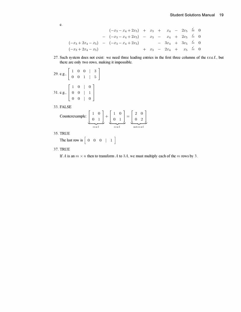
27. Such system does not exist: we need three leading entries in the first three columns of the r.r.e.f., but
there are only two rows, making it impossible.
29. e.g.,
[1 0 0 | 3
0 0 1 | 5
]
31. e.g.,
⎡⎢⎣ 1 0 | 0
0 0 | 1
0 0 | 0
⎤⎥⎦33. FALSE
Counterexample:
[1 0
0 1
]︸ ︷︷ ︸
r.r.e.f.
+
[1 0
0 1
]︸ ︷︷ ︸
r.r.e.f.
=
[2 0
0 2
]︸ ︷︷ ︸
not r.r.e.f.
35. TRUE
The last row is[0 0 0 | 1
]37. TRUE
If A is anm× n then to transform A to 3A, we must multiply each of the m rows by 3.
20 Student Solutions Manual
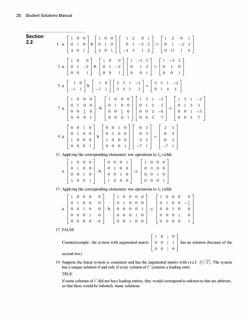
Section
2.2 1. a.
⎡⎢⎣ 1 0 0
0 1 0
4 0 1
⎤⎥⎦ b.
⎡⎢⎣ 1 0 0
0 1 0
4 0 1
⎤⎥⎦⎡⎢⎣ 1 2 0 1
0 1 −2 2
−4 3 1 2
⎤⎥⎦ =
⎡⎢⎣ 1 2 0 1
0 1 −2 2
0 11 1 6
⎤⎥⎦
3. a.
⎡⎢⎣ 1 0 0
0 1 −2
0 0 1
⎤⎥⎦ b.
⎡⎢⎣ 1 0 0
0 1 −2
0 0 1
⎤⎥⎦⎡⎢⎣ 1 −3 5
0 1 2
0 0 1
⎤⎥⎦ =
⎡⎢⎣ 1 −3 5
0 1 0
0 0 1
⎤⎥⎦5. a.
[1 0
−1 1
]b.
[1 0
−1 1
][2 3 1 −2
2 4 5 2
]=
[2 3 1 −2
0 1 4 4
]
7. a.
⎡⎢⎢⎢⎢⎣1 0 0 0
0 1 0 0
0 0 12 0
0 0 0 1
⎤⎥⎥⎥⎥⎦ ; b.⎡⎢⎢⎢⎢⎣
1 0 0 0
0 1 0 0
0 0 12 0
0 0 0 1
⎤⎥⎥⎥⎥⎦⎡⎢⎢⎢⎢⎣
1 3 1 −2
0 1 2 5
0 0 2 −6
0 0 3 7
⎤⎥⎥⎥⎥⎦ =
⎡⎢⎢⎢⎢⎣1 3 1 −2
0 1 2 5
0 0 1 −3
0 0 3 7
⎤⎥⎥⎥⎥⎦
9. a.
⎡⎢⎢⎢⎢⎣0 0 1 0
0 1 0 0
1 0 0 0
0 0 0 1
⎤⎥⎥⎥⎥⎦ b.
⎡⎢⎢⎢⎢⎣0 0 1 0
0 1 0 0
1 0 0 0
0 0 0 1
⎤⎥⎥⎥⎥⎦⎡⎢⎢⎢⎢⎣
0 2
0 3
2 5
−7 1
⎤⎥⎥⎥⎥⎦ =
⎡⎢⎢⎢⎢⎣2 5
0 3
0 2
−7 1
⎤⎥⎥⎥⎥⎦11. Applying the corresponding elementary row operations to I4 yields
a.
⎡⎢⎢⎢⎢⎣1 0 0 0
0 1 0 0
0 0 1 0
5 0 0 1
⎤⎥⎥⎥⎥⎦ ; b.⎡⎢⎢⎢⎢⎣
0 0 0 1
0 1 0 0
0 0 1 0
1 0 0 0
⎤⎥⎥⎥⎥⎦ ; c.⎡⎢⎢⎢⎢⎣
1 0 0 0
0 3 0 0
0 0 1 0
0 0 0 1
⎤⎥⎥⎥⎥⎦13. Applying the corresponding elementary row operations to I5 yields
a.
⎡⎢⎢⎢⎢⎢⎢⎣1 0 0 0 0
0 1 0 0 0
0 0 1 0 0
0 0 0 1 0
0 0 0 0 −6
⎤⎥⎥⎥⎥⎥⎥⎦ ; b.⎡⎢⎢⎢⎢⎢⎢⎣
1 0 0 0 0
0 1 0 0 0
0 0 0 0 1
0 0 0 1 0
0 0 1 0 0
⎤⎥⎥⎥⎥⎥⎥⎦ ; c.⎡⎢⎢⎢⎢⎢⎢⎣
1 0 0 0 0
0 1 0 0 − 12
0 0 1 0 0
0 0 0 1 0
0 0 0 0 1
⎤⎥⎥⎥⎥⎥⎥⎦17. FALSE
Counterexample: the system with augmented matrix
⎡⎢⎣ 1 0 | 0
0 0 | 1
0 0 | 0
⎤⎥⎦ has no solution (because of the
second row)
19. Suppose the linear system is consistent and has the augmented matrix with r.r.e.f. [C|−→d ]. The system
has a unique solution if and only if every column of C contains a leading entry.
TRUE
If some columns of C did not have leading entries, they would correspond to unknowns that are arbitrary,
so that there would be infinitely many solutions.
Student Solutions Manual 21
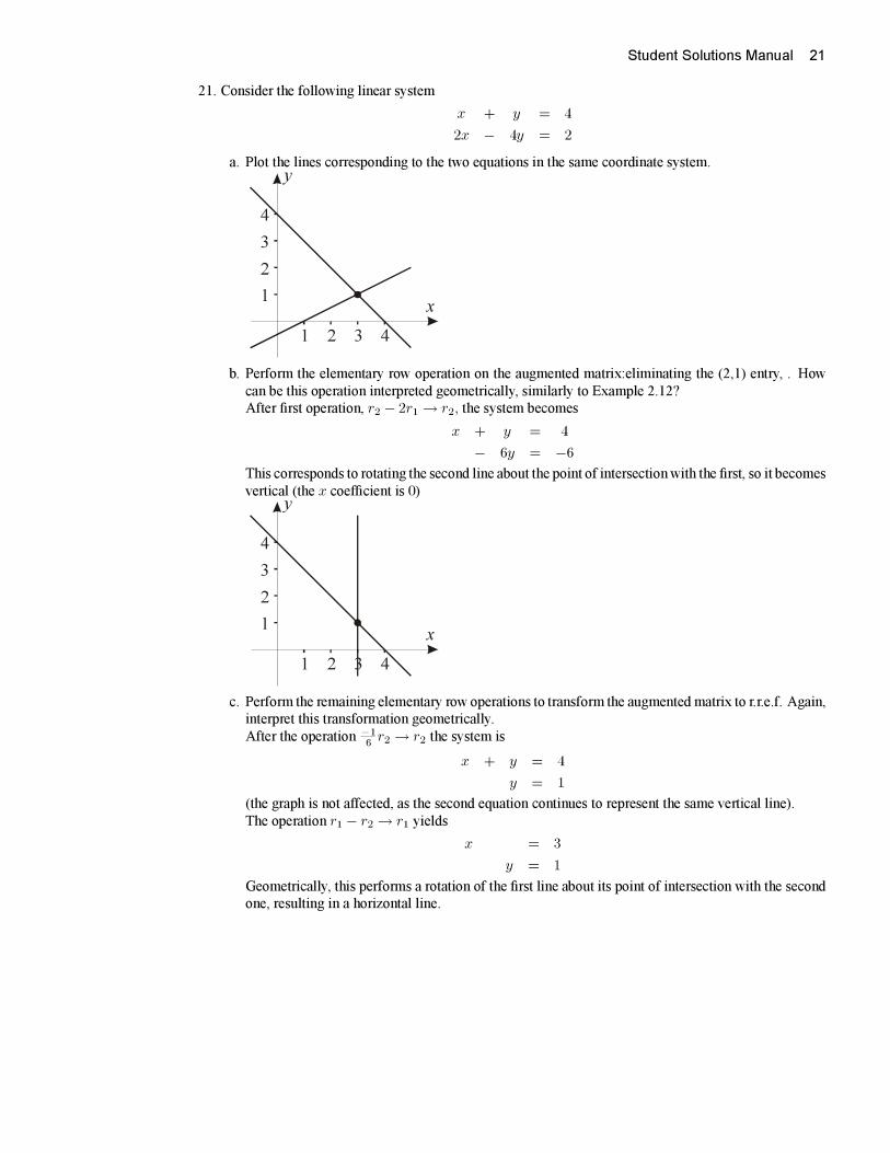
21. Consider the following linear system
x + y = 4
2x − 4y = 2
a. Plot the lines corresponding to the two equations in the same coordinate system.
x
1
1
2
2 3
3
4
4
y
b. Perform the elementary row operation on the augmented matrix:eliminating the (2,1) entry, . How
can be this operation interpreted geometrically, similarly to Example 2.12?
After first operation, r2 − 2r1 → r2, the system becomes
x + y = 4
− 6y = −6
This corresponds to rotating the second line about the point of intersectionwith the first, so it becomes
vertical (the x coefficient is 0)
x
1
1
2
2 3
3
4
4
y
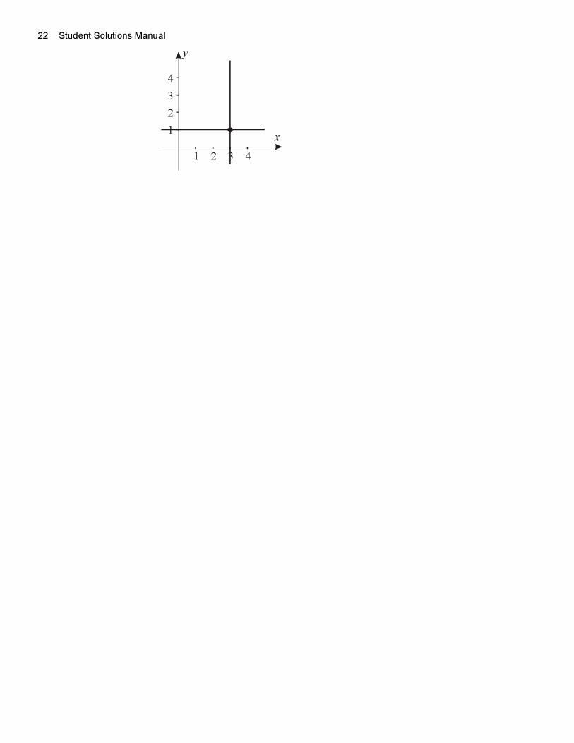
c. Perform the remaining elementary row operations to transform the augmented matrix to r.r.e.f. Again,
interpret this transformation geometrically.
After the operation −16r2 → r2 the system is
x + y = 4
y = 1
(the graph is not affected, as the second equation continues to represent the same vertical line).
The operation r1 − r2 → r1 yields
x = 3
y = 1
Geometrically, this performs a rotation of the first line about its point of intersection with the second
one, resulting in a horizontal line.
22 Student Solutions Manual
x
1
1
2
2 3
3
4
4
y
Student Solutions Manual 23
Section
2.3
NOTE, For most solutions in this section, the individual row operations required can be obtained using the
Linear Algebra Toolkit.
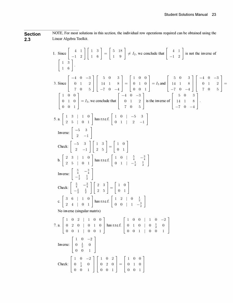
1. Since
[4 1
−1 2
][1 3
1 6
]=
[5 18
1 9
]�= I2, we conclude that
[4 1
−1 2
]is not the inverse of[
1 3
1 6
].
3. Since
⎡⎢⎣ −4 0 −3
0 1 2
7 0 5
⎤⎥⎦⎡⎢⎣ 5 0 3
14 1 8
−7 0 −4
⎤⎥⎦ =
⎡⎢⎣ 1 0 0
0 1 0
0 0 1
⎤⎥⎦ = I3 and
⎡⎢⎣ 5 0 3
14 1 8
−7 0 −4
⎤⎥⎦⎡⎢⎣ −4 0 −3
0 1 2
7 0 5
⎤⎥⎦ =
⎡⎢⎣ 1 0 0
0 1 0
0 0 1
⎤⎥⎦ = I3, we conclude that
⎡⎢⎣ −4 0 −3
0 1 2
7 0 5
⎤⎥⎦ is the inverse of
⎡⎢⎣ 5 0 3
14 1 8
−7 0 −4
⎤⎥⎦ .
5. a.
[1 3 | 1 0
2 5 | 0 1
]has r.r.e.f.
[1 0 | −5 3
0 1 | 2 −1
]
Inverse:
[−5 3
2 −1
]
Check:
[−5 3
2 −1
][1 3
2 5
]=
[1 0
0 1
]
b.
[2 3 | 1 0
2 5 | 0 1
]has r.r.e.f.
[1 0 | 5
4 − 34
0 1 | −12
12
]
Inverse:
[54
− 34
−12
12
]
Check:
[54 −3
4
− 12
12
][2 3
2 5
]=
[1 0
0 1
]
c.
[3 6 | 1 0
2 4 | 0 1
]has r.r.e.f.
[1 2 | 0 1
2
0 0 | 1 −32
]No inverse (singular matrix)
7. a.
⎡⎢⎣ 1 0 2 | 1 0 0
0 2 0 | 0 1 0
0 0 1 | 0 0 1
⎤⎥⎦ has r.r.e.f.
⎡⎢⎣ 1 0 0 | 1 0 −2
0 1 0 | 0 12 0
0 0 1 | 0 0 1
⎤⎥⎦
Inverse:
⎡⎢⎣ 1 0 −2
0 12
0
0 0 1
⎤⎥⎦
Check:
⎡⎢⎣ 1 0 −2
0 12 0
0 0 1
⎤⎥⎦⎡⎢⎣ 1 0 2
0 2 0
0 0 1
⎤⎥⎦ =
⎡⎢⎣ 1 0 0
0 1 0
0 0 1
⎤⎥⎦
24 Student Solutions Manual
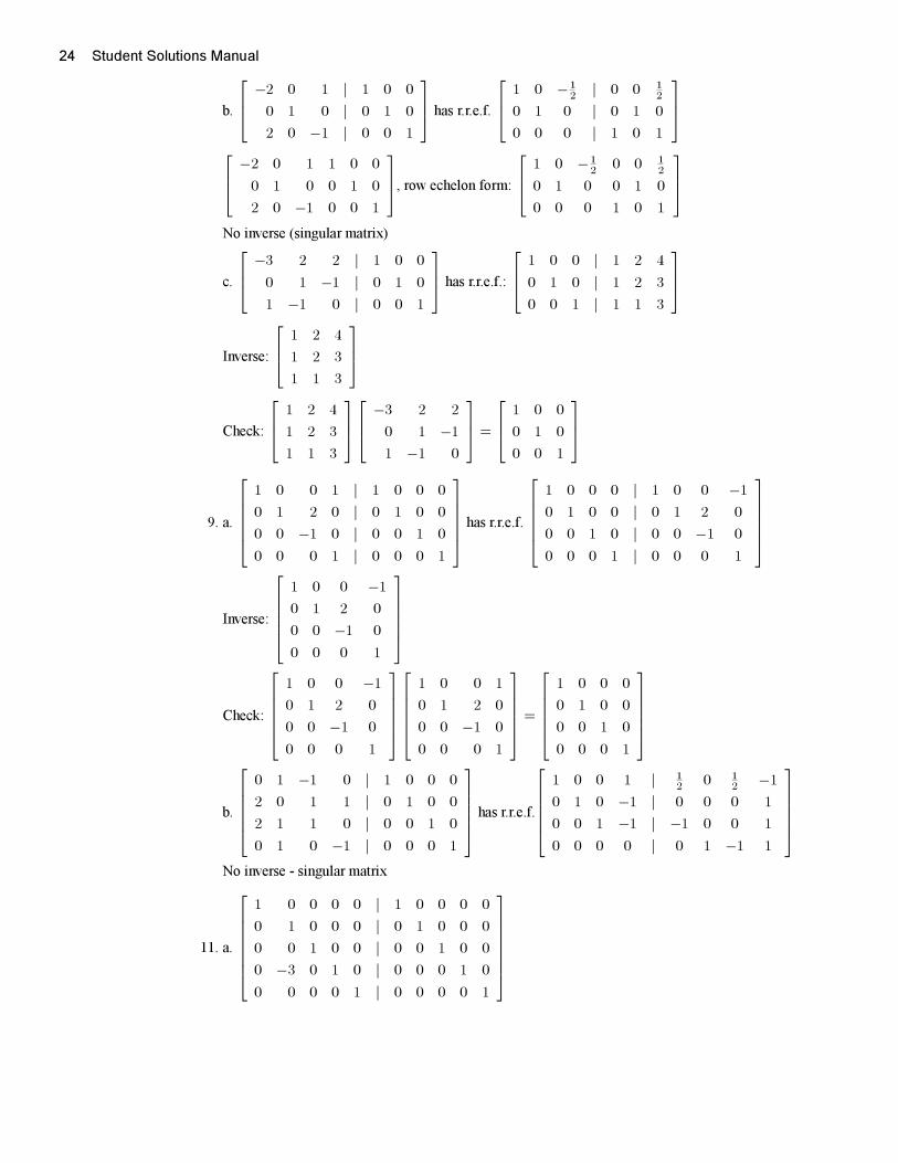
b.
⎡⎢⎣ −2 0 1 | 1 0 0
0 1 0 | 0 1 0
2 0 −1 | 0 0 1
⎤⎥⎦ has r.r.e.f.
⎡⎢⎣ 1 0 −12 | 0 0 1
2
0 1 0 | 0 1 0
0 0 0 | 1 0 1
⎤⎥⎦⎡⎢⎣ −2 0 1 1 0 0
0 1 0 0 1 0
2 0 −1 0 0 1
⎤⎥⎦, row echelon form:
⎡⎢⎣ 1 0 −12
0 0 12
0 1 0 0 1 0
0 0 0 1 0 1
⎤⎥⎦No inverse (singular matrix)
c.
⎡⎢⎣ −3 2 2 | 1 0 0
0 1 −1 | 0 1 0
1 −1 0 | 0 0 1
⎤⎥⎦ has r.r.e.f.:
⎡⎢⎣ 1 0 0 | 1 2 4
0 1 0 | 1 2 3
0 0 1 | 1 1 3
⎤⎥⎦
Inverse:
⎡⎢⎣ 1 2 4
1 2 3
1 1 3
⎤⎥⎦
Check:
⎡⎢⎣ 1 2 4
1 2 3
1 1 3
⎤⎥⎦⎡⎢⎣ −3 2 2
0 1 −1
1 −1 0
⎤⎥⎦ =
⎡⎢⎣ 1 0 0
0 1 0
0 0 1
⎤⎥⎦
9. a.
⎡⎢⎢⎢⎢⎣1 0 0 1 | 1 0 0 0
0 1 2 0 | 0 1 0 0
0 0 −1 0 | 0 0 1 0
0 0 0 1 | 0 0 0 1
⎤⎥⎥⎥⎥⎦ has r.r.e.f.
⎡⎢⎢⎢⎢⎣1 0 0 0 | 1 0 0 −1
0 1 0 0 | 0 1 2 0
0 0 1 0 | 0 0 −1 0
0 0 0 1 | 0 0 0 1
⎤⎥⎥⎥⎥⎦
Inverse:
⎡⎢⎢⎢⎢⎣1 0 0 −1
0 1 2 0
0 0 −1 0
0 0 0 1
⎤⎥⎥⎥⎥⎦
Check:
⎡⎢⎢⎢⎢⎣1 0 0 −1
0 1 2 0
0 0 −1 0
0 0 0 1
⎤⎥⎥⎥⎥⎦⎡⎢⎢⎢⎢⎣
1 0 0 1
0 1 2 0
0 0 −1 0
0 0 0 1
⎤⎥⎥⎥⎥⎦ =
⎡⎢⎢⎢⎢⎣1 0 0 0
0 1 0 0
0 0 1 0
0 0 0 1
⎤⎥⎥⎥⎥⎦
b.
⎡⎢⎢⎢⎢⎣0 1 −1 0 | 1 0 0 0
2 0 1 1 | 0 1 0 0
2 1 1 0 | 0 0 1 0
0 1 0 −1 | 0 0 0 1
⎤⎥⎥⎥⎥⎦ has r.r.e.f.
⎡⎢⎢⎢⎢⎣1 0 0 1 | 1
2 0 12 −1
0 1 0 −1 | 0 0 0 1
0 0 1 −1 | −1 0 0 1
0 0 0 0 | 0 1 −1 1
⎤⎥⎥⎥⎥⎦No inverse - singular matrix
11. a.
⎡⎢⎢⎢⎢⎢⎢⎣1 0 0 0 0 | 1 0 0 0 0
0 1 0 0 0 | 0 1 0 0 0
0 0 1 0 0 | 0 0 1 0 0
0 −3 0 1 0 | 0 0 0 1 0
0 0 0 0 1 | 0 0 0 0 1
⎤⎥⎥⎥⎥⎥⎥⎦
Student Solutions Manual 25
has r.r.e.f.
⎡⎢⎢⎢⎢⎢⎢⎣1 0 0 0 0 | 1 0 0 0 0
0 1 0 0 0 | 0 1 0 0 0
0 0 1 0 0 | 0 0 1 0 0
0 0 0 1 0 | 0 3 0 1 0
0 0 0 0 1 | 0 0 0 0 1
⎤⎥⎥⎥⎥⎥⎥⎦
Inverse
⎡⎢⎢⎢⎢⎢⎢⎣1 0 0 0 0
0 1 0 0 0
0 0 1 0 0
0 3 0 1 0
0 0 0 0 1
⎤⎥⎥⎥⎥⎥⎥⎦
Check
⎡⎢⎢⎢⎢⎢⎢⎣1 0 0 0 0
0 1 0 0 0
0 0 1 0 0
0 3 0 1 0
0 0 0 0 1
⎤⎥⎥⎥⎥⎥⎥⎦
⎡⎢⎢⎢⎢⎢⎢⎣1 0 0 0 0
0 1 0 0 0
0 0 1 0 0
0 −3 0 1 0
0 0 0 0 1
⎤⎥⎥⎥⎥⎥⎥⎦�=
⎡⎢⎢⎢⎢⎢⎢⎣1 0 0 0 0
0 1 0 0 0
0 0 1 0 0
0 0 0 1 0
0 0 0 0 1
⎤⎥⎥⎥⎥⎥⎥⎦
b.
⎡⎢⎢⎢⎢⎢⎢⎢⎢⎢⎣
1 0 0 0 0 0 | 1 0 0 0 0 0
0 1 0 0 0 0 | 0 1 0 0 0 0
0 0 1 0 0 0 | 0 0 1 0 0 0
0 0 0 1 0 0 | 0 0 0 1 0 0
0 0 0 0 4 0 | 0 0 0 0 1 0
0 0 0 0 0 1 | 0 0 0 0 0 1
⎤⎥⎥⎥⎥⎥⎥⎥⎥⎥⎦
has r.r.e.f.
⎡⎢⎢⎢⎢⎢⎢⎢⎢⎢⎣
1 0 0 0 0 0 | 1 0 0 0 0 0
0 1 0 0 0 0 | 0 1 0 0 0 0
0 0 1 0 0 0 | 0 0 1 0 0 0
0 0 0 1 0 0 | 0 0 0 1 0 0
0 0 0 0 1 0 | 0 0 0 0 14
0
0 0 0 0 0 1 | 0 0 0 0 0 1
⎤⎥⎥⎥⎥⎥⎥⎥⎥⎥⎦
Inverse:
⎡⎢⎢⎢⎢⎢⎢⎢⎢⎢⎣
1 0 0 0 0 0
0 1 0 0 0 0
0 0 1 0 0 0
0 0 0 1 0 0
0 0 0 0 14 0
0 0 0 0 0 1
⎤⎥⎥⎥⎥⎥⎥⎥⎥⎥⎦
Check:
⎡⎢⎢⎢⎢⎢⎢⎢⎢⎢⎣
1 0 0 0 0 0
0 1 0 0 0 0
0 0 1 0 0 0
0 0 0 1 0 0
0 0 0 0 14
0
0 0 0 0 0 1
⎤⎥⎥⎥⎥⎥⎥⎥⎥⎥⎦
⎡⎢⎢⎢⎢⎢⎢⎢⎢⎢⎣
1 0 0 0 0 0
0 1 0 0 0 0
0 0 1 0 0 0
0 0 0 1 0 0
0 0 0 0 4 0
0 0 0 0 0 1
⎤⎥⎥⎥⎥⎥⎥⎥⎥⎥⎦=
⎡⎢⎢⎢⎢⎢⎢⎢⎢⎢⎣
1 0 0 0 0 0
0 1 0 0 0 0
0 0 1 0 0 0
0 0 0 1 0 0
0 0 0 0 1 0
0 0 0 0 0 1
⎤⎥⎥⎥⎥⎥⎥⎥⎥⎥⎦13.
[1 −1
−4 3
], inverse:
[−3 −1
−4 −1
]
26 Student Solutions Manual[−3 −1
−4 −1
][1
−3
]=
[0
−1
]
15.
⎡⎢⎣ 0 3 2
−1 2 1
1 0 0
⎤⎥⎦, inverse:⎡⎢⎣ 0 0 1
−1 2 2
2 −3 −3
⎤⎥⎦⎡⎢⎣ 0 0 1
−1 2 2
2 −3 −3
⎤⎥⎦⎡⎢⎣ 0
−1
−1
⎤⎥⎦ =
⎡⎢⎣ −1
−4
6
⎤⎥⎦17. Inverse transformation: reflection with respect to the y-axis (same as F )
A = A−1 =
[−1 0
0 1
].
[−1 0
0 1
][−1 0
0 1
]�=
[1 0
0 1
]19. Not invertible
21. a. (AB)−1 = B−1A−1 =
⎡⎢⎣ 0 3 1
3 1 3
1 3 0
⎤⎥⎦⎡⎢⎣ 1 2 −1
1 2 0
1 1 1
⎤⎥⎦ =
⎡⎢⎣ 4 7 1
7 11 0
4 8 −1
⎤⎥⎦b.(AT)−1
= (A−1)T =
⎡⎢⎣ 1 1 1
2 2 1
−1 0 1
⎤⎥⎦c. Premultiplying both sides of A−→x =
⎡⎢⎣ 3
1
1
⎤⎥⎦ by A−1 yields A−1A−→x = A−1
⎡⎢⎣ 3
1
1
⎤⎥⎦ ,therefore−→x = A−1
⎡⎢⎣ 3
1
1
⎤⎥⎦ =
⎡⎢⎣ 1 2 −1
1 2 0
1 1 1
⎤⎥⎦⎡⎢⎣ 3
1
1
⎤⎥⎦ =
⎡⎢⎣ 4
5
5
⎤⎥⎦ .d. From the equivalent conditions, invertible n×n matrices must be row equivalent to In. Since A and
B are both invertible, they are both row equivalent to In, and consequently are row equivalent to
each other.
23. a. (BTA)−1 = A−1(BT )−1 = A−1(B−1)T =
⎡⎢⎢⎢⎢⎣0 1 0 1
2 0 1 0
0 2 0 1
2 0 2 0
⎤⎥⎥⎥⎥⎦⎡⎢⎢⎢⎢⎣
1 0 1 0
1 1 1 0
0 1 1 1
0 1 0 1
⎤⎥⎥⎥⎥⎦ =
⎡⎢⎢⎢⎢⎣1 2 1 1
2 1 3 1
2 3 2 1
2 2 4 2
⎤⎥⎥⎥⎥⎦ .
b. ((A−1)−1)−1 = A−1 =
⎡⎢⎢⎢⎢⎣0 1 0 1
2 0 1 0
0 2 0 1
2 0 2 0
⎤⎥⎥⎥⎥⎦
c.(B2)−1
= (BB)−1 = B−1B−1 =
⎡⎢⎢⎢⎢⎣1 1 0 0
0 1 1 1
1 1 1 0
0 0 1 1
⎤⎥⎥⎥⎥⎦⎡⎢⎢⎢⎢⎣
1 1 0 0
0 1 1 1
1 1 1 0
0 0 1 1
⎤⎥⎥⎥⎥⎦ =
⎡⎢⎢⎢⎢⎣1 2 1 1
1 2 3 2
2 3 2 1
1 1 2 1
⎤⎥⎥⎥⎥⎦d. (AB−1)−1(BA−1)−1 = (B−1)−1A−1(A−1)−1B−1 = BA−1AB−1 = BI4B
−1 = BB−1 =
Student Solutions Manual 27
I4 =
⎡⎢⎢⎢⎢⎣1 0 0 0
0 1 0 0
0 0 1 0
0 0 0 1
⎤⎥⎥⎥⎥⎦ .27. TRUE
LHS = (A−1B−1)T = (B−1)T (A−1)T
RHS = (ATBT )−1 = (BT )−1(AT )−1
29. FALSE
By the equivalent conditions, A is nonsingular if and only if A−→x =
[1
2
]has a unique solution.
31. TRUE
By the equivalent conditions, if A is row equivalent to I3 then A−→x =
⎡⎢⎣ 9
7
3
⎤⎥⎦ has a unique solution
(therefore, it must be consistent).
33. TRUE
By the equivalent conditions, all nonsingular 5× 5 matrices are row equivalent to I5, therefore, they are
also row equivalent to each other.
28 Student Solutions Manual
Section
2.4 1. The augmented matrix
[2 −1 0 | 0
5 −2 −2 | 0
]has the r.r.e.f.:
[1 0 −2 | 0
0 1 −4 | 0
].
x1 = 2x3, x2 = 4x3, x3 is arbitrary.
Let x3 = 1 : 2 N2O5 → 4 NO2 + O2
3. The augmented matrix
⎡⎢⎣ 10 0 −1 0 | 0
16 0 0 −1 | 0
0 2 0 −1 | 0
⎤⎥⎦ has the r.r.e.f.:
⎡⎢⎣ 1 0 0 − 116 | 0
0 1 0 −12 | 0
0 0 1 −58 | 0
⎤⎥⎦x1 = 1
16x4, x2 = 12x4, x3 = 5
8x4, x4 is arbitrary
Let x4 = 16 (any smaller positive integer would lead to at least some fractions):
C10H16 + 8Cl2 → 10C+16HCl
5. The augmented matrix
⎡⎢⎣ 6 −2 −1 | 0
12 −6 0 | 0
6 −1 −1 | 0
⎤⎥⎦ has the r.r.e.f.:
⎡⎢⎣ 1 0 0 | 0
0 1 0 | 0
0 0 1 | 0
⎤⎥⎦The system has only one solution: x1 = x2 = x3 = 0.
The reaction equation cannot be balanced.
(It is rather fortunate that the process of fermentation of glucose produces ethanol and carbon dioxide
CO2, rather than carbonmonoxide CO.)
7. The augmented matrix
⎡⎢⎢⎢⎢⎢⎢⎣3 0 −1 0 | 0
1 0 0 −1 | 0
4 0 0 −4 | 0
0 1 0 −1 | 0
0 3 −1 0 | 0
⎤⎥⎥⎥⎥⎥⎥⎦ has the r.r.e.f.:
⎡⎢⎢⎢⎢⎢⎢⎣1 0 0 −1 | 0
0 1 0 −1 | 0
0 0 1 −3 | 0
0 0 0 0 | 0
0 0 0 0 | 0
⎤⎥⎥⎥⎥⎥⎥⎦x1 = x4, x2 = x4, x3 = 3x4, x4 is arbitrary
Let x4 = 1 : Rb3PO4+CrCl3 → 3RbCl+CrPO4
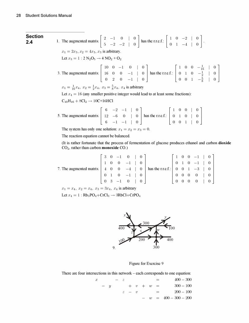
9.
400
100
100
200 400
300
300
v
xy
zw
Figure for Exercise 9
There are four intersections in this network – each corresponds to one equation:
x − z = 400− 300
− y + v + w = 300− 100
z − v = 200− 100
− w = 400− 300− 200
Student Solutions Manual 29
The augmentedmatrix
⎡⎢⎢⎢⎢⎣1 0 −1 0 0 100
0 −1 0 1 1 200
0 0 1 −1 0 100
0 0 0 0 −1 −100
⎤⎥⎥⎥⎥⎦ has the r.r.e.f.:⎡⎢⎢⎢⎢⎣
1 0 0 −1 0 200
0 1 0 −1 0 −100
0 0 1 −1 0 100
0 0 0 0 1 100
⎤⎥⎥⎥⎥⎦ .Therefore, every solution satisfies
x = 200 + v
y = −100 + v
z = 100 + v
v = arbitrary
w = 100
There are infinitely many solutions, some of which involve negative values, which are not allowed in this
model. Examples of solutions with all positive numbers can be constructed by taking any v > 100, e.g.for v = 200 :
x = 400, y = 100, z = 300, v = 200, w = 100.
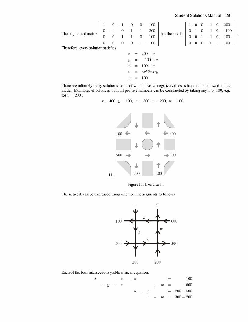
11.
600
300
200200
500
100
Figure for Exercise 11
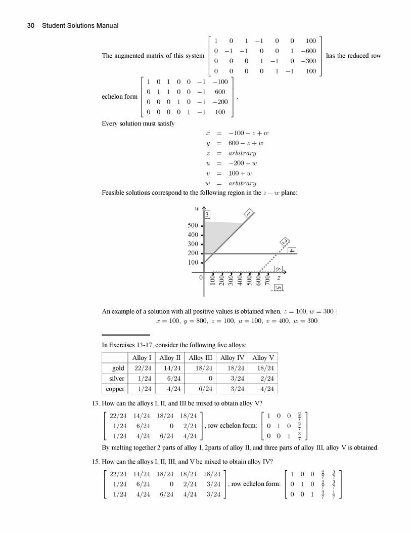
The network can be expressed using oriented line segments as follows
600
300
200200
500
100
x y
z
u
v
w
Each of the four intersections yields a linear equation:
x + z − u = 100
− y − z + w = −600
u − v = 200− 500
v − w = 300− 200
30 Student Solutions Manual
The augmented matrix of this system
⎡⎢⎢⎢⎢⎣1 0 1 −1 0 0 100
0 −1 −1 0 0 1 −600
0 0 0 1 −1 0 −300
0 0 0 0 1 −1 100
⎤⎥⎥⎥⎥⎦ has the reduced row
echelon form
⎡⎢⎢⎢⎢⎣1 0 1 0 0 −1 −100
0 1 1 0 0 −1 600
0 0 0 1 0 −1 −200
0 0 0 0 1 −1 100
⎤⎥⎥⎥⎥⎦ .Every solution must satisfy
x = −100− z +w
y = 600− z +w
z = arbitrary
u = −200 +w
v = 100 +w
w = arbitrary
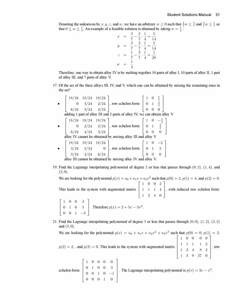
Feasible solutions correspond to the following region in the z −w plane:
z
w
3
5
2
6
4
1
0
100
100
300
300
500
500
200
200
400400
600
700
An example of a solution with all positive values is obtained when. z = 100, w = 300 :
x = 100, y = 800, z = 100, u = 100, v = 400, w = 300
In Exercises 13-17, consider the following five alloys:
Alloy I Alloy II Alloy III Alloy IV Alloy V
gold 22/24 14/24 18/24 18/24 18/24
silver 1/24 6/24 0 3/24 2/24
copper 1/24 4/24 6/24 3/24 4/24
13. How can the alloys I, II, and III be mixed to obtain alloy V?⎡⎢⎣ 22/24 14/24 18/24 18/24
1/24 6/24 0 2/24
1/24 4/24 6/24 4/24
⎤⎥⎦, row echelon form:
⎡⎢⎣ 1 0 0 27
0 1 0 27
0 0 1 37
⎤⎥⎦By melting together 2 parts of alloy I, 2parts of alloy II, and three parts of alloy III, alloy V is obtained.
15. How can the alloys I, II, III, and V be mixed to obtain alloy IV?⎡⎢⎣ 22/24 14/24 18/24 18/24 18/24
1/24 6/24 0 2/24 3/24
1/24 4/24 6/24 4/24 3/24
⎤⎥⎦, row echelon form:
⎡⎢⎣ 1 0 0 27
37
0 1 0 27
37
0 0 1 37
17
⎤⎥⎦
Student Solutions Manual 31
Denoting the unknowns by x, y, z, and w, we have an arbitrary w ≥ 0 such that 27w ≤ 3
7 and 37w ≤ 1
7 so
that 0 ≤ w ≤ 13 . An example of a feasible solution is obtained by taking w = 1
4 :
x =3
7− 2
7· 14=
5
14
y =3
7− 2
7· 14=
5
14
z =1
7− 3
7· 14=
1
28
w =1
4
Therefore, one way to obtain alloy IV is by melting together 10 parts of alloy I, 10 parts of alloy II, 1 part
of alloy III, and 7 parts of alloy V.
17. Of the set of the three alloys III, IV, and V, which one can be obtained by mixing the remaining ones in
the set?
•
⎡⎢⎣ 18/24 18/24 18/24
0 3/24 2/24
6/24 3/24 4/24
⎤⎥⎦, row echelon form:
⎡⎢⎣ 1 0 13
0 1 23
0 0 0
⎤⎥⎦adding 1 part of alloy III and 2 parts of alloy IV, we can obtain alloy V
•
⎡⎢⎣ 18/24 18/24 18/24
0 2/24 3/24
6/24 4/24 3/24
⎤⎥⎦, row echelon form:
⎡⎢⎣ 1 0 − 12
0 1 32
0 0 0
⎤⎥⎦alloy IV cannot be obtained by mixing alloy III and alloy V
•
⎡⎢⎣ 18/24 18/24 18/24
3/24 2/24 0
3/24 4/24 6/24
⎤⎥⎦, row echelon form:
⎡⎢⎣ 1 0 −2
0 1 3
0 0 0
⎤⎥⎦alloy III cannot be obtained by mixing alloy IV and alloy V.
19. Find the Lagrange interpolating polynomial of degree 2 or less that passes through (0, 2), (1,4), and(2,0).
We are looking for the polynomial p(x) = a0 +a1x+a2x2 such that p(0) = 2, p(1) = 4, and p(2) = 0.
This leads to the system with augmented matrix
⎡⎢⎣ 1 0 0 2
1 1 1 4
1 2 4 0
⎤⎥⎦, with reduced row echelon form:
⎡⎢⎣ 1 0 0 2
0 1 0 5
0 0 1 −3
⎤⎥⎦ . Therefore p(x) = 2 + 5x− 3x2.
21. Find the Lagrange interpolating polynomial of degree 3 or less that passes through (0, 0), (1,2), (2,2)and (3, 0).
We are looking for the polynomial p(x) = a0 + a1x + a2x2 + a3x
3 such that p(0) = 0, p(1) = 2,
p(2) = 2, . and p(3) = 0. This leads to the system with augmented matrix
⎡⎢⎢⎢⎢⎣1 0 0 0 0
1 1 1 1 2
1 2 4 8 2
1 3 9 27 0
⎤⎥⎥⎥⎥⎦, row
echelon form:
⎡⎢⎢⎢⎢⎣1 0 0 0 0
0 1 0 0 3
0 0 1 0 −1
0 0 0 1 0
⎤⎥⎥⎥⎥⎦ . The Lagrange interpolating polynomial is p(x) = 3x− x2.
32 Student Solutions Manual
23. Hermite interpolating polynomial p(x) of degree 2n− 1 satisfies the conditions
p(xi) = yi and p′(xi) = di for i = 0, 1, . . . , n
where the values xi, yi , and di are given (and x′is are distinct). Use a linear system to determine
p(x) = a0 + a1x+ a2x2 + a3x
3 such that
p(0) = 2, p′(0) = 1, p(1) = 4, and p′(1) = 0.
The augmented matrix of the system
⎡⎢⎢⎢⎢⎣1 0 0 0 2
0 1 0 0 1
1 1 1 1 4
0 1 2 3 0
⎤⎥⎥⎥⎥⎦ has the r.r.e.f.:
⎡⎢⎢⎢⎢⎣1 0 0 0 2
0 1 0 0 1
0 0 1 0 4
0 0 0 1 −3
⎤⎥⎥⎥⎥⎦ .Therefore, p(x) = 2 + x+4x2 − 3x3.
25. If possible, find a polynomial p(x) = a0 + a1x+ a2x2 + a3x
3 such that
p(0) = 1, p′(0) = 1, p′(2) = 0, and p(3) = 2.
Note that this is not a Hermite interpolating polynomial – e.g., at x = 2, the first derivative is specified,but the value is not. This is an example of a Hermite-Birkhoff interpolation problem, and it may or may
not have a solution (even if it does, the solution need not be unique).
The augmented matrix of the system
⎡⎢⎢⎢⎢⎣1 0 0 0 1
0 1 0 0 1
0 1 4 12 0
1 3 9 27 2
⎤⎥⎥⎥⎥⎦ has the r.r.e.f.:
⎡⎢⎢⎢⎢⎣1 0 0 0 0
0 1 0 0 0
0 0 1 3 0
0 0 0 0 1
⎤⎥⎥⎥⎥⎦ .Therefore, there is no solution to this system.
27. p0(1) = 3 : b0 + c0 + d0 = 3− 2
p1(2) = 0 : b1 + c1 + d1 = 0− 3
p′0(1) = p′1(1) : b0 + 2c0 +3d0 = b1
p′′0 (1) = p′′1 (1) : 2c0 +6d0 = 2c1
p′′0 (0) = 0 : 2c0 = 0
p′′1 (2) = 0 : 2c1 + 6d1 = 0⎡⎢⎢⎢⎢⎢⎢⎢⎢⎢⎣
1 1 1 0 0 0 1
0 0 0 1 1 1 −3
1 2 3 −1 0 0 0
0 2 6 0 −2 0 0
0 2 0 0 0 0 0
0 0 0 0 2 6 0
⎤⎥⎥⎥⎥⎥⎥⎥⎥⎥⎦has the reduced row echelon form:
⎡⎢⎢⎢⎢⎢⎢⎢⎢⎢⎣
1 0 0 0 0 0 2
0 1 0 0 0 0 0
0 0 1 0 0 0 −1
0 0 0 1 0 0 −1
0 0 0 0 1 0 −3
0 0 0 0 0 1 1
⎤⎥⎥⎥⎥⎥⎥⎥⎥⎥⎦p0(x) = 2 + 2x− x3
p1(x) = 3− 1(x− 1) − 3(x− 1)2 + 1(x− 1)3
Check: p0(1) = 2 + 2− 1 = 3
p1(2) = 3− 1− 3 + 1 = 0
p′0(x) = 2− 3x2; p′0(1) = −1; p′1(x) = −1− 6(x− 1) + 3(x− 1)2; p′1(1) = −1
p′′0 (x) = −6x; p′′0 (1) = −6; p′′1 (x) = −6 + 6(x− 1); p′′1 (1) = −6
p′′0 (0) = 0
p′′1 (2) = −6 + 6 = 0.
29. r2 − ar1 → r2
If 6 − 3a �= 0, i.e. a �= 2, then the system has a unique solution (a leading entry corresponds to each
unknown)
Student Solutions Manual 33
If 6 − 3a = 0, i.e. a = 2, then the matrix becomes
[1 3 1
0 0 0
], - the system has infinitely many
solutions
(i) impossible
(ii) a �= 2
(iii) a = 2
31. r1 ↔ r2[−1 a 0
a 1 0
]−r1 → r1[
1 −a 0
a 1 0
]r2 − ar1 → r2[
1 −a 0
0 1 + a2 0
](i) impossible
(ii) for all real a values
(iii) impossible (1 + a2 cannot equal 0 for any real a).
33. r2 − (a− 1)r1 → r2[1 a+ 1 0
0 3− (a+1)(a − 1) b
]=
[1 a+ 1 0
0 4− a2 b
]If 4 − a2 �= 0, i.e. a �= ±2 then the system has a unique solution (a leading entry corresponds to each
unknown)
If 4− a2 = 0, i.e. a = ±2 then
• if b = 0, the system has many solutions,
• if b �= 0, the system has no solution.
(i) a = ±2 and b �= 0(ii) a �= ±2(iii) a = ±2 and b = 0.
35.• If a = b = 0 then there are infinitely many solutions.
• If a = 0 and b �= 0 thenr1 ↔ r2[
b 0 0
0 b 0
]1br1 → r1
1br2 → r2[1 0 0
0 1 0
]Unique solution
• If a �= 0 then1ar1 → r1[1 b
a0
b a 0
]r2 − br1 → r2
34 Student Solutions Manual[1 b
a0
0 a− b2
a0
]If a− b2
a= 0, i.e. a2−b2
a= (a−b)(a+b)
a= 0 then there are infinitely many solutions
Otherwise, there is a unique solution.
(i) impossible
(ii) a �= b and a �= −b,(iii) a = b or a = −b
41. a. L =
[1 0
5 1
], U =
[1 5
0 −23
]; LU =
[1 5
5 2
]
b. Solve
[1 0
5 1
][y1
y2
]=
[−2
13
]by forward substitution
y1 = −2
y2 = 13− 5y1 = 23
Solve
[1 5
0 −23
][x1
x2
]=
[−2
23
]by backsubstitution
x2 = −1
x1 = −2− 5x2 = 3
43. a. L =
⎡⎢⎢⎢⎢⎣1 0 0 0
1 1 0 0
2 3 1 0
0 −1 2 1
⎤⎥⎥⎥⎥⎦ ; U =
⎡⎢⎢⎢⎢⎣1 0 0 5
0 1 0 −4
0 0 1 2
0 0 0 −8
⎤⎥⎥⎥⎥⎦ ; LU =
⎡⎢⎢⎢⎢⎣1 0 0 5
1 1 0 1
2 3 1 0
0 −1 2 0
⎤⎥⎥⎥⎥⎦
b. Solve
⎡⎢⎢⎢⎢⎣1 0 0 0
1 1 0 0
2 3 1 0
0 −1 2 1
⎤⎥⎥⎥⎥⎦⎡⎢⎢⎢⎢⎣
y1
y2
y3
y4
⎤⎥⎥⎥⎥⎦ =
⎡⎢⎢⎢⎢⎣1
0
−3
−3
⎤⎥⎥⎥⎥⎦ by forward substitution
y1 = 1
y2 = −y1 = −1
y3 = −3− 2y1 − 3y2 = −2
y4 = −3 + y2 − 2y3 = 0
Solve
⎡⎢⎢⎢⎢⎣1 0 0 5
0 1 0 −4
0 0 1 2
0 0 0 −8
⎤⎥⎥⎥⎥⎦⎡⎢⎢⎢⎢⎣
x1
x2
x3
x4
⎤⎥⎥⎥⎥⎦ =
⎡⎢⎢⎢⎢⎣1
−1
−2
0
⎤⎥⎥⎥⎥⎦ by backsubstitution
x4 = 0
x3 = −2− 2x4 = −2
x2 = −1+ 4x4 = −1
x1 = 1− 5x4 = 1
45. P =
⎡⎢⎣ 0 1 0
1 0 0
0 0 1
⎤⎥⎦ ; L =
⎡⎢⎣ 1 0 0
−3 1 0
−4 2 1
⎤⎥⎦ ; U =
⎡⎢⎣ −1 1 0
0 3 1
0 0 −1
⎤⎥⎦
Verify: PA =
⎡⎢⎣ 0 1 0
1 0 0
0 0 1
⎤⎥⎦⎡⎢⎣ 3 0 1
−1 1 0
4 2 1
⎤⎥⎦ =
⎡⎢⎣ −1 1 0
3 0 1
4 2 1
⎤⎥⎦

Student Solutions Manual 35
LU =
⎡⎢⎣ 1 0 0
−3 1 0
−4 2 1
⎤⎥⎦⎡⎢⎣ −1 1 0
0 3 1
0 0 −1
⎤⎥⎦ =
⎡⎢⎣ −1 1 0
3 0 1
4 2 1
⎤⎥⎦
36 Student Solutions Manual
Section
3.11. a. det
[1 3
2 1
]i. Expand along the first row:
detA = (1) det[1]− 3 det[2] = −5
ii. Let A =
[1 3
2 1
]r2 − 2r1 → r2
A1 =
[1 3
0 −5
], detA1 = detA
detA1 = (1)(−5) and−5 = detA1 = detATherefore, detA = −5.ii. detA = (1)(1)− (3)(2) = 1− 6 = −5.
b. det
⎡⎢⎣ 1 3 0
0 3 5
2 0 1
⎤⎥⎦i Expand along the first row:
detA = (1)((3)(1)− (5)(0))− 3((0)(1)− (5)(2)) + 0= 3 + 30 = 33.
ii. Let A =
⎡⎢⎣ 1 3 0
0 3 5
2 0 1
⎤⎥⎦r2 − 2r1 → r2
A1 =
⎡⎢⎣ 1 3 0
0 3 5
0 −6 1
⎤⎥⎦ , detA1 = detA
r3 + 2r2 → r3
A2 =
⎡⎢⎣ 1 3 0
0 3 5
0 0 11
⎤⎥⎦ , detA2 = detA1
detA2 = (1)(3)(11) and33 = detA2 = detA1 = detATherefore, detA = 33.iii. detA = (1)(3)(1) + (3)(5)(2) + (0)(0)(0)− (0)(3)(2) − (1)(5)(0)− (3)(0)(1)= 3 + 30 + 0− 0− 0− 0 = 33.
c. det
⎡⎢⎣ 9 7 2
8 6 7
0 0 0
⎤⎥⎦i. Expand along the third row: detA = 0− 0 + 0 = 0.ii. r2 − 8
9r1 → r2
A1 =
⎡⎢⎣ 9 7 2
0 −29
479
0 0 0
⎤⎥⎦detA1 = (9)(−2
9 )(0) = 0 = detAiii. detA = (9)(6)(0) + (7)(7)(0) + (2)(8)(0)− (2)(6)(0) − (9)(7)(0)− (7)(8)(0)= 0 + 0 + 0− 0− 0− 4 = 0.
Student Solutions Manual 37
3. a. det
⎡⎢⎢⎢⎢⎣1 1 0 3
0 0 1 0
0 2 2 4
−2 0 0 3
⎤⎥⎥⎥⎥⎦i. Expand along the second row:
detA = −0 + 0− 1 det
⎡⎢⎣ 1 1 3
0 2 4
−2 0 3
⎤⎥⎦+ 0
= −[6− 8 + 0 + 12− 0− 0] = −10
ii. Let A =
⎡⎢⎢⎢⎢⎣1 1 0 3
0 0 1 0
0 2 2 4
−2 0 0 3
⎤⎥⎥⎥⎥⎦r4 + 2r1 → r4
A1 =
⎡⎢⎢⎢⎢⎣1 1 0 3
0 0 1 0
0 2 2 4
0 2 0 9
⎤⎥⎥⎥⎥⎦ , detA1 = detA
r2 + 2r1 → r2
A2 =
⎡⎢⎢⎢⎢⎣1 1 0 3
0 0 1 0
0 2 2 4
0 2 0 9
⎤⎥⎥⎥⎥⎦ , detA2 = detA1
r3 ↔ r2
A3 =
⎡⎢⎢⎢⎢⎣1 1 0 3
0 2 2 4
0 0 1 0
0 2 0 9
⎤⎥⎥⎥⎥⎦ , detA3 = −detA2
r4 − r2 → r4
A4 =
⎡⎢⎢⎢⎢⎣1 1 0 3
0 2 2 4
0 0 1 0
0 0 −2 5
⎤⎥⎥⎥⎥⎦ , detA4 = detA3
r4 + 2r3 → r4
A5 =
⎡⎢⎢⎢⎢⎣1 1 0 3
0 2 2 4
0 0 1 0
0 0 0 5
⎤⎥⎥⎥⎥⎦ , detA5 = detA4
detA5 = (1)(2)(1)(5) and10 = detA5 = detA4 = detA3 = −detA2 = −detA1 = − detATherefore, detA = −10.
b. det
⎡⎢⎢⎢⎢⎢⎢⎣0 2 0 0 0
2 0 1 2 0
0 0 −1 0 0
0 1 0 1 3
4 0 2 0 0
⎤⎥⎥⎥⎥⎥⎥⎦i. Expand along the first row:
38 Student Solutions Manual
detA = 0− 2 det
⎡⎢⎢⎢⎢⎣2 1 2 0
0 −1 0 0
0 0 1 3
4 2 0 0
⎤⎥⎥⎥⎥⎦+ 0− 0 + 0
Expand the 4× 4 determinant along the second row:
detA = −2(0− 1det
⎡⎢⎣ 2 2 0
0 1 3
4 0 0
⎤⎥⎦+ 0− 0)
= 2[0 + 24 + 0− 0− 0− 0) = 48
ii. Let A =
⎡⎢⎢⎢⎢⎢⎢⎣0 2 0 0 0
2 0 1 2 0
0 0 −1 0 0
0 1 0 1 3
4 0 2 0 0
⎤⎥⎥⎥⎥⎥⎥⎦r2 ↔ r1
A1 =
⎡⎢⎢⎢⎢⎢⎢⎣2 0 1 2 0
0 2 0 0 0
0 0 −1 0 0
0 1 0 1 3
4 0 2 0 0
⎤⎥⎥⎥⎥⎥⎥⎦ , detA1 = − detA
r5 − 2r1 → r5
A2 =
⎡⎢⎢⎢⎢⎢⎢⎣2 0 1 2 0
0 2 0 0 0
0 0 −1 0 0
0 1 0 1 3
0 0 0 −4 0
⎤⎥⎥⎥⎥⎥⎥⎦ , detA2 = detA1
r4 − 12r2 → r4
A3 =
⎡⎢⎢⎢⎢⎢⎢⎣2 0 1 2 0
0 2 0 0 0
0 0 −1 0 0
0 0 0 1 3
0 0 0 −4 0
⎤⎥⎥⎥⎥⎥⎥⎦ , detA3 = detA2
r5 + 4r4 → r5
A4 =
⎡⎢⎢⎢⎢⎢⎢⎣2 0 1 2 0
0 2 0 0 0
0 0 −1 0 0
0 0 0 1 3
0 0 0 0 12
⎤⎥⎥⎥⎥⎥⎥⎦ , detA4 = detA3
detA4 = (2)(2)(−1)(1)(12) and−48 = detA4 = detA3 = detA2 = detA1 = −detATherefore, detA = 48.
5. a. det
[0 −2
3 −7
]= (0)(−7)− (−2)(3) = 0 + 6 = 6.
b. det
⎡⎢⎣ 2 0 1
−3 1 2
0 2 1
⎤⎥⎦Expand along the first row:
Student Solutions Manual 39
2(−1)1+1 det
[1 2
2 1
]+ 0 + 1(−1)1+3 det
[−3 1
0 2
]= 2(−3)− 6= −12
c. det
⎡⎢⎣ 2 1 3
2 −1 −2
1 1 2
⎤⎥⎦Expand along the first row:
2(−1)1+1 det
[−1 −2
1 2
]+1(−1)1+2 det
[2 −2
1 2
]
+3(−1)1+3 det
[2 −1
1 1
]= 2(0) − 1(6) + 3(3)= 3
7. a. det
⎡⎢⎢⎢⎢⎣2 1 0 3
4 0 2 0
1 −1 1 2
0 0 −1 2
⎤⎥⎥⎥⎥⎦Expand along the fourth row:
0 + 0 + (−1)(−1)4+3 det
⎡⎢⎣ 2 1 3
4 0 0
1 −1 2
⎤⎥⎦+ 2(−1)4+4 det
⎡⎢⎣ 2 1 0
4 0 2
1 −1 1
⎤⎥⎦= −20 + 2(2)= −16
b. det
⎡⎢⎢⎢⎢⎢⎢⎣−1 0 1 0 1
0 1 −1 0 1
1 0 1 2 −1
0 1 1 0 1
0 0 1 0 0
⎤⎥⎥⎥⎥⎥⎥⎦Expand along the fourth column:
0 + 0 + 2(−1)3+4 det
⎡⎢⎢⎢⎢⎣−1 0 1 1
0 1 −1 1
0 1 1 1
0 0 1 0
⎤⎥⎥⎥⎥⎦+ 0 + 0
now, expand along the first column:
= −2((−1)(−1)1+1 det
⎡⎢⎣ 1 −1 1
1 1 1
0 1 0
⎤⎥⎦)= −2(−1)(0)= 0
9. Let A =
⎡⎢⎣−→v1 T
−→v2 T
−→v3 T
⎤⎥⎦ is a 3× 3 matrix such that detA = 6. Calculate the determinant of
a.
⎡⎢⎣−→v1T
−→v2T +2−→v1T
−→v3T
⎤⎥⎦
40 Student Solutions Manual
Answer: 6 (adding a multiple of one row to another does not change the determinant)
b.
⎡⎢⎣−→v3T
−→v2T
−→v1T
⎤⎥⎦Answer: −6 (interchanging two rows reverses the sign of the determinant)
c.
⎡⎢⎣ −→v1T
−→v1T
−→v3T
⎤⎥⎦Answer: 0 (If we subtract row 1 from row 2, the second row becomes a zero row)
d. A−1
Answer 1/6.det(A−1) = 1/detA
e. 2A.Every time a row is multiplied by a factor, the determinant is also multiplied by the same factor.
Therefore,
det(2A) = (2)(2)(2)(6) = 48.
11. Let A =
⎡⎢⎣ 2 0 0
6 −1 0
0 4 3
⎤⎥⎦ and let B be a matrix such that B−1 =
⎡⎢⎣ −1 8 8
0 2 3
0 0 −2
⎤⎥⎦ . Calculate the
determinant of
a. AT
Answer: −6 (AT is upper triangular)
b. Answer: −6detA = detAT - see above
c. AB.Answer: −3
2det(AB) = detAdetB = detA 1
detB−1 = −64 = −3
2
13. a. det(BTA2) = det(BT ) (det(A))2 = det(B) (det(A))2 = (5)(−3)2 = 45
b. det(A−1B) = 1det(A) det(B) =
(1−3
)(5) = −5
3
c. det(3A) = 33 det(A) = (27)(−3) = −81 (every time a row is multiplied by k, the determinant is
also multiplied by k - since all three rows are scaled by k, the determinant is multiplied by k · k ·k =k3)
d. det((2B)−1) = 1det(2B) = 1
23 det(B) =1
(8)(5) =140
e. det(ATBA−1) = det(AT ) det(B) det(A−1) = det(A) det(B)(
1det(A)
)= det(B) = 5
f. det((A−1B)−1(BA)T ) = det(B−1AATBT ) = 1det(B)
det(A) det(A) det(B) = (det(A))2 = 9
13. If all entries of a square matrix A are positive then detA > 0.
FALSE
Counterexample: det
[1 2
2 1
]= 1− 4 = −3.
15. If one of the columns of an n × n matrix A is a linear combination of the remaining columns, then
detA = 0.
TRUE
If one of the columns of an n × n matrix A is a linear combination of the remaining columns, then the
columns of A are L.D. From the equivalent statements, detA = 0.
Student Solutions Manual 41
17. If A is anm× n matrix and B is an n×m matrix then det(AB) = det(BA).
FALSE
Counterexample
A =
[1
2
], B =
[2 3
].
det(AB) = det
[2 3
4 6
]= 0 while
det(BA) = det [8] = 8.
19. If A is a 3× 3 matrix with detA = 2 then rank A = 3.
TRUE
From the equivalent statements, rank A = n is equivalent to detA �= 0.
42 Student Solutions Manual
Section
3.21.
3x1 − x2 = 3
−2x1 + 3x2 = 5
detA = det
[3 −1
−2 3
]= 9− 2 = 7 �= 0, therefore, the system has a unique solution, which can be
found using Cramer’s rule.
detA1 = det
[3 −1
5 3
]= 9+ 5 = 14.
detA2 = det
[3 3
−2 5
]= 15+ 6 = 21.
Therefore,
x1 = detA1
detA = 147 = 2.
x2 = detA2
detA = 217 = 3.
3.
2x1 − x2 = 1
−4x1 + 2x2 = 6
detA = det
[2 −1
−4 2
]= 4 − 4 = 0, therefore, the system either has many solutions or none.
Cramer’s rule cannot be used here.
5.
x1 + 2x2 + 3x3 = 1
x1 + x2 = −1
x2 + 3x3 = 0
detA = det
⎡⎢⎣ 1 2 3
1 1 0
0 1 3
⎤⎥⎦ = 0 therefore, the system either has many solutions or none. Cramer’s rule
cannot be used here.
7.
x1 + 2x2 − x3 = 2
3x2 − 2x3 = 1
2x1 − x2 + x3 = 1
detA = det
⎡⎢⎣ 1 2 −1
0 3 −2
2 −1 1
⎤⎥⎦ = −1 �= 0, therefore, the system has a unique solution, which can be
found using Cramer’s rule.
detA1 = det
⎡⎢⎣ 2 2 −1
1 3 −2
1 −1 1
⎤⎥⎦ = 0.
Student Solutions Manual 43
detA2 = det
⎡⎢⎣ 1 2 −1
0 1 −2
2 1 1
⎤⎥⎦ = −3.
detA3 = det
⎡⎢⎣ 1 2 2
0 3 1
2 −1 1
⎤⎥⎦ = −4.
Therefore,
x1 = detA1
detA= 0
−1= 0.
x2 = detA2
detA = −3−1 = 3.
x3 = detA3
detA = −4−1 = 4.
9. a.
[−1 2
3 1
]A11 = (−1)1+1 det [1] = 1
A12 = (−1)1+2 det [3] = −3
A21 = (−1)2+1 det [2] = −2
A22 = (−1)2+2 det [−1] = −1
adj A =
[A11 A21
A12 A22
]=
[1 −2
−3 −1
].
A adj A =
[−1 2
3 1
][1 −2
−3 −1
]=
[−7 0
0 −7
]= (detA) I2.
b.
⎡⎢⎣ 1 1 2
−2 1 −1
0 2 −3
⎤⎥⎦A11 = (−1)1+1 det
[1 −1
2 −3
]= −1
A12 = (−1)1+2 det
[−2 −1
0 −3
]= −6
A13 = (−1)1+3 det
[−2 1
0 2
]= −4
A21 = (−1)2+1 det
[1 2
2 −3
]= 7
A22 = (−1)2+2 det
[1 2
0 −3
]= −3
A23 = (−1)2+3 det
[1 1
0 2
]= −2
A31 = (−1)3+1 det
[1 2
1 −1
]= −3
A32 = (−1)3+2 det
[1 2
−2 −1
]= −3
44 Student Solutions Manual
A33 = (−1)3+3 det
[1 1
−2 1
]= 3
adjA =
⎡⎢⎣ A11 A21 A31
A12 A22 A32
A13 A23 A33
⎤⎥⎦ =
⎡⎢⎣ −1 7 −3
−6 −3 −3
−4 −2 3
⎤⎥⎦⎡⎢⎣ 1 1 2
−2 1 −1
0 2 −3
⎤⎥⎦⎡⎢⎣ −1 7 −3
−6 −3 −3
−4 −2 3
⎤⎥⎦ =
⎡⎢⎣ −15 0 0
0 −15 0
0 0 −15
⎤⎥⎦= (detA) I3
c.
⎡⎢⎣ 2 0 −1
0 1 0
−4 0 2
⎤⎥⎦A11 = (−1)1+1 det
[1 0
0 2
]= 2
A12 = (−1)1+2 det
[0 0
−4 2
]= 0
A13 = (−1)1+3 det
[0 1
−4 0
]= 4
A21 = (−1)2+1 det
[0 −1
0 2
]= 0
A22 = (−1)2+2 det
[2 −1
−4 2
]= 0
A23 = (−1)2+3 det
[2 0
−4 0
]= 0
A31 = (−1)3+1 det
[0 −1
1 0
]= 1
A32 = (−1)3+2 det
[2 −1
0 0
]= 0
A33 = (−1)3+3 det
[2 0
0 1
]= 2
adjA =
⎡⎢⎣ A11 A21 A31
A12 A22 A32
A13 A23 A33
⎤⎥⎦ =
⎡⎢⎣ 2 0 1
0 0 0
4 0 2
⎤⎥⎦
A adjA =
⎡⎢⎣ 2 0 −1
0 1 0
−4 0 2
⎤⎥⎦⎡⎢⎣ 2 0 1
0 0 0
4 0 2
⎤⎥⎦
=
⎡⎢⎣ 0 0 0
0 0 0
0 0 0
⎤⎥⎦ = (detA) I3
Student Solutions Manual 45
11. P (5, 2), Q(−1, 3), and R(4,0).
−→PQ =
[−1− 5
3− 2
]=
[−6
1
]
−→PR =
[4− 5
0− 2
]=
[−1
−2
]The triangle has the area:
12
∣∣∣∣∣det[
−6 −1
1 −2
]∣∣∣∣∣ = 12 |12 + 1| = 13
2 .
13. For each of the three transformations of the letter “F” depicted in Exercise 16 on p.52, visually estimate
the determinant based on how the transformation affects the shape. (All determinants here will be integers
between −4 and 4). Confirm that the same determinant is calculated from the correct matrix.
(a) det = 4 (each dimension is doubled) - matches detA2
(b) det = 1 (dimensions remain unchanged) - matches detA1
(c ) det = 1 (the size of the parallelogram is the same as that of the original rectangle) - matches detA3.
15. Adjoint of a diagonal matrix is diagonal.
TRUE
If i > j then Aij involves a determinant of an (n − 1) × (n − 1) lower triangular matrix B for which
bjj = 0, therefore detB = 0.
Likewise, when i < j then Aij involves a determinant of an (n − 1)× (n− 1) upper triangular matrix
B for which bii = 0, therefore detB = 0.
17. For all real numbers k and n× n matrices A, adj(kA) = kadjA.
FALSE
Let A be invertible. Then adj A = (det A)A−1. Also, adj (kA) = (det kA)(kA)−1.
However, det(kA) = kn detA, and (kA)−1 = 1kA−1. Therefore adj (kA) = kn−1adjA.
19. If A is singular then adjA does not exist.
FALSE
Adjoint of every square matrix exists.
46 Student Solutions Manual
Section
4.11. Property 2.
LHS =
[a1
a2
]+
[b1
b2
]=
[a1
b2
]
RHS =
[b1
b2
]+
[a1
a2
]=
[b1
a2
]Generally, LHS �= RHS ⇒Property does not hold.
Property 3.
LHS = (
[a1
a2
]+
[b1
b2
]) +
[c1
c2
]=
[a1
b2
]+
[c1
c2
]=
[a1
c2
]
RHS =
[a1
a2
]+ (
[b1
b2
]+
[c1
c2
]) =
[a1
a2
]+
[b1
c2
]=
[a1
c2
].
LHS = RHS ⇒Property holds
Property 7.
LHS = k(
[a1
a2
]+
[b1
b2
]) = k
[a1
b2
]=
[ka1
kb2
]
RHS = k
[a1
a2
]+ k
[b1
b2
]=
[ka1
ka2
]+
[kb1
kb2
]=
[ka1
kb2
]LHS = RHS ⇒Property holds
Property 8
LHS = (c + d)
[a1
a2
]=
[(c+ d)a1
(c+ d)a2
]
RHS = c
[a1
a2
]+ d
[a1
a2
]=
[ca1
ca2
]+
[da1
da2
]=
[ca1
da2
]Generally, LHS �= RHS ⇒Property does not hold.
3. Property 7.
LHS = k(
⎡⎢⎣ a1
a2
a3
⎤⎥⎦+
⎡⎢⎣ b1
b2
b3
⎤⎥⎦) = k
⎡⎢⎣ a1 + b1
a2 + b2
a3 + b3
⎤⎥⎦ =
⎡⎢⎣ a1 + b1
a2 + b2
a3 + b3
⎤⎥⎦
RHS = k
⎡⎢⎣ a1
a2
a3
⎤⎥⎦+ k
⎡⎢⎣ b1
b2
b3
⎤⎥⎦ =
⎡⎢⎣ a1
a2
a3
⎤⎥⎦+
⎡⎢⎣ b1
b2
b3
⎤⎥⎦ =
⎡⎢⎣ a1 + b1
a2 + b2
a3 + b3
⎤⎥⎦LHS = RHS ⇒Property holds
Property 8.
LHS = (c + d)
⎡⎢⎣ a1
a2
a3
⎤⎥⎦ =
⎡⎢⎣ a1
a2
a3
⎤⎥⎦
Student Solutions Manual 47
RHS = c
⎡⎢⎣ a1
a2
a3
⎤⎥⎦+ d
⎡⎢⎣ a1
a2
a3
⎤⎥⎦ =
⎡⎢⎣ a1
a2
a3
⎤⎥⎦+
⎡⎢⎣ a1
a2
a3
⎤⎥⎦ =
⎡⎢⎣ 2a1
2a2
2a3
⎤⎥⎦Generally, LHS �= RHS ⇒Property does not hold.
Property 9.
LHS = (cd)
⎡⎢⎣ a1
a2
a3
⎤⎥⎦ =
⎡⎢⎣ a1
a2
a3
⎤⎥⎦
RHS = c(d
⎡⎢⎣ a1
a2
a3
⎤⎥⎦) = c
⎡⎢⎣ a1
a2
a3
⎤⎥⎦ =
⎡⎢⎣ a1
a2
a3
⎤⎥⎦LHS = RHS ⇒Property holds
Property 10.
LHS = 1
⎡⎢⎣ a1
a2
a3
⎤⎥⎦ =
⎡⎢⎣ a1
a2
a3
⎤⎥⎦LHS = RHS ⇒Property holds
5. Property 2.
LHS =
[a 0
0 a
]+
[b 0
0 b
]=
[a+ b 0
0 a+ b
]
RHS =
[b 0
0 b
]+
[a 0
0 a
]=
[b+ a 0
0 b+ a
]LHS = RHS ⇒Property holds
Property 3.
LHS = (
[a 0
0 a
]+
[b 0
0 b
])+
[c 0
0 c
]=
[a+ b 0
0 a+ b
]+
[c 0
0 c
]=
[a+ b+ c 0
0 a + b+ c
]
RHS =
[a 0
0 a
]+(
[b 0
0 b
]+
[c 0
0 c
]) =
[a 0
0 a
]+
[b+ c 0
0 b+ c
]=
[a+ b+ c 0
0 a + b+ c
]LHS = RHS ⇒Property holds
Property 4 holds with the zero vector
[0 0
0 0
].
Property 9
LHS = (cd)
[a 0
0 a
]=
[cda 0
0 cda
]
RHS = c(d
[a 0
0 a
]) = c
[da 0
0 da
]=
[cda 0
0 cda
]LHS = RHS ⇒Property holds
Property 10.
1
[a 0
0 a
]=
[a 0
0 a
]

48 Student Solutions Manual
LHS = RHS ⇒Property holds
7. Property 4 fails: cannot find
[z1
z2
]independent of a1 and a2 such that
[a1
a2
]+
[z1
z2
]=
[a1
a2
]for all a1 and a2.
Also, property 10 fails (1
[a1
a2
]=
[a1
0
]generally
�=[
a1
a2
])
9. All ten properties hold. (Using the theory in Section 3.2., this can be shown to be a subspace of R2,therefore, it is a vector space.)
Student Solutions Manual 49
Section
4.2 1. No, does not contain
[0
0
]. (Violates property a.)
3. Yes, satisfies all three properties. Also,W =span{[
0
1
]}.
5. No, violates property c.:
e.g. (−2)
[3
0
]=
[−6
0
]is not inW.
7. Yes, satisfies all three properties. Also,W =span{
⎡⎢⎣ 1
0
1
⎤⎥⎦ ,⎡⎢⎣ 0
1
−1
⎤⎥⎦}.9. Yes, satisfies all three properties.
a. 0 + 2(0)− 0�= 0
b. Taking two vectors inW,
⎡⎢⎣ x1
x2
x3
⎤⎥⎦ and
⎡⎢⎣ y1
y2
y3
⎤⎥⎦ such that
x1 + 2x2 − x3 = 0 and y1 + 2y2 − y3 = 0
the sum
⎡⎢⎣ x1 + y1
x2 + y2
x3 + y3
⎤⎥⎦ satisfies
(x1 + y1) + 2(x2 + y2)− (x3 + y3) = (x1 + 2x2 − x3) + (y1 + 2y2 − y3) = 0 + 0�= 0
which means it is inW.
c. Taking a scalar multiple of a vector inW : c
⎡⎢⎣ x1
x2
x3
⎤⎥⎦ with x1 + 2x2 − x3 = 0, we obtain the vector
⎡⎢⎣ cx1
cx2
cx3
⎤⎥⎦ that satisfies
cx1 + 2cx2 − cx3 = c(x1 + 2x2 − x3) = (c)(0) = 0.
Note that this space is the solution space of the homogeneous equation x1 + 2x2 − x3 = 0.
11. Yes,W =span{1 + t+ t2}.
13. No, does not contain
[0 0
0 0
]. (Violates property a.)
15. No, violates property b. ,e.g.
⎡⎢⎣ 1 0 0 0
0 1 0 0
0 0 1 0
⎤⎥⎦+⎡⎢⎣ 1 0 0 0
0 1 0 0
0 0 1 0
⎤⎥⎦ =
⎡⎢⎣ 2 0 0 0
0 2 0 0
0 0 2 0
⎤⎥⎦ is outside the
set.
17. Yes. It satisfies the three properties:
50 Student Solutions Manual
• Property a holds since the function f(x) ≡ 0 is continuous (it’s in the set)
• Property b holds because a sum of two continuous functions, f + g is also continuous.
• Property c holds because a scalar multiple of a continuous function f, cf, is also continuous for everyscalar c.
19. No. It violates property c., e.g., while the function f(x) = x is in the set, the scalar multiple (−1)f is
not.
21. Yes.
The equation c1
[1
1
]+c2
[2
1
]=
[d1
d2
]is equivalent to a linear system with the augmented matrix[
1 2 | d1
1 1 | d2
].The r.r.e.f.,
[1 0 | −d1 + 2d2
0 1 | d1 − d2
]contains no row of the form [ 0 · · ·0 | nonzero],
therefore the system is consistent for all d1 and d2.
23. No.
The equation c1
⎡⎢⎣ 1
3
0
⎤⎥⎦ + c2
⎡⎢⎣ 0
1
−2
⎤⎥⎦ =
⎡⎢⎣ d1
d2
d3
⎤⎥⎦ is equivalent to a linear system with the augmented
matrix
⎡⎢⎣ 1 0 | d1
3 1 | d2
0 −2 | d3
⎤⎥⎦ .After the row operations r2 − 3r1 → r2 and r3 + 2r2 → r3,
⎡⎢⎣ 1 0 | d1
0 1 | −3d1 + d2
0 0 | −6d1 + 2d2 + d3
⎤⎥⎦ has the third row in the form [ 0 · · · 0 | nonzero], therefore the system
is inconsistent for some d1, d2 and d3.
25. Yes.
The equation c1
⎡⎢⎣ 0
0
0
⎤⎥⎦+c2
⎡⎢⎣ 1
0
2
⎤⎥⎦+c3
⎡⎢⎣ 0
2
−1
⎤⎥⎦+c4
⎡⎢⎣ 1
0
0
⎤⎥⎦ =
⎡⎢⎣ d1
d2
d3
⎤⎥⎦ is equivalent to a linear system
with the augmentedmatrix
⎡⎢⎣ 0 1 0 1 | d1
0 0 2 0 | d2
0 2 −1 0 | d3
⎤⎥⎦ .The r.r.e.f.,⎡⎢⎣ 0 1 0 0 | 1
4d2 +12d3
0 0 1 0 | 12d2
0 0 0 1 | d1 − 14d2 − 1
2d3
⎤⎥⎦contains no row of the form [ 0 · · · 0 | nonzero], therefore the system is consistent for all d1, d2 and d3.
27. Yes.
The equation
c1(1− 3t2
)+ c2t+ c3
(−1 + 2t2)= d1 + d2t+ d3t
2
is equivalent to a linear system
c1 − c3 = d1
c2 = d2
−3c1 + 2c3 = d3
with the augmented matrix
⎡⎢⎣ 1 0 −1 | d1
0 1 0 | d2
−3 0 2 | d3
⎤⎥⎦ . The r.r.e.f.,⎡⎢⎣ 1 0 0 −2d1 − d3
0 1 0 d2
0 0 1 −3d1 − d3
⎤⎥⎦ contains
no row of the form [ 0 · · · 0 | nonzero], therefore the system is consistent for all d1, d2 and d3.
29. No.
Student Solutions Manual 51
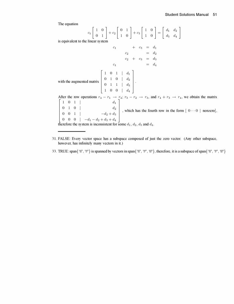
The equation
c1
[1 0
0 1
]+ c2
[0 1
1 0
]+ c3
[1 0
1 0
]=
[d1 d2
d3 d4
]is equivalent to the linear system
c1 + c3 = d1
c2 = d2
c2 + c3 = d3
c1 = d4
with the augmented matrix
⎡⎢⎢⎢⎢⎣1 0 1 | d1
0 1 0 | d2
0 1 1 | d3
1 0 0 | d4
⎤⎥⎥⎥⎥⎦ .After the row operations r4 − r1 → r4; r3 − r2 → r3, and r4 + r3 → r4, we obtain the matrix⎡⎢⎢⎢⎢⎣
1 0 1 | d1
0 1 0 | d2
0 0 1 | −d2 + d3
0 0 0 | −d1 − d2 + d3 + d4
⎤⎥⎥⎥⎥⎦ , which has the fourth row in the form [ 0 · · ·0 | nonzero],
therefore the system is inconsistent for some d1, d2, d3 and d4.
31. FALSE: Every vector space has a subspace composed of just the zero vector. (Any other subspace,
however, has infinitely many vectors in it.)
33. TRUE: span{−→u ,−→v } is spanned by vectors in span{−→u ,−→v ,−→w }, therefore, it is a subspace of span{−→u ,−→v ,−→w }
52 Student Solutions Manual
Section
4.3
NOTE: Refer to the Linear Algebra Toolkit for the details involved in solving these problems, including the
individual elementary row operations.
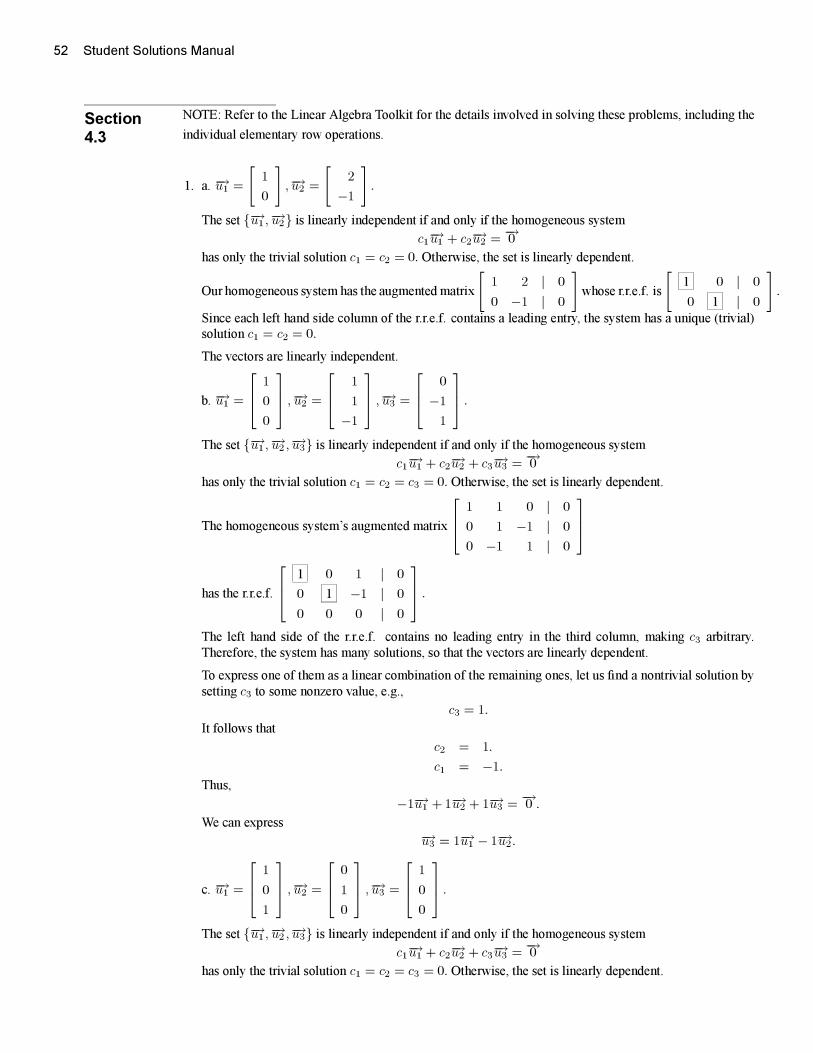
1. a. −→u1 =
[1
0
],−→u2 =
[2
−1
].
The set {−→u1 ,−→u2} is linearly independent if and only if the homogeneous system
c1−→u1 + c2−→u2 =−→0
has only the trivial solution c1 = c2 = 0. Otherwise, the set is linearly dependent.
Ourhomogeneous system has the augmented matrix
[1 2 | 0
0 −1 | 0
]whose r.r.e.f. is
[1 0 | 0
0 1 | 0
].
Since each left hand side column of the r.r.e.f. contains a leading entry, the system has a unique (trivial)
solution c1 = c2 = 0.
The vectors are linearly independent.
b. −→u1 =
⎡⎢⎣ 1
0
0
⎤⎥⎦ ,−→u2 =
⎡⎢⎣ 1
1
−1
⎤⎥⎦ ,−→u3 =
⎡⎢⎣ 0
−1
1
⎤⎥⎦ .The set {−→u1 ,−→u2 ,−→u3} is linearly independent if and only if the homogeneous system
c1−→u1 + c2−→u2 + c3−→u3 =−→0
has only the trivial solution c1 = c2 = c3 = 0. Otherwise, the set is linearly dependent.
The homogeneous system’s augmented matrix
⎡⎢⎣ 1 1 0 | 0
0 1 −1 | 0
0 −1 1 | 0
⎤⎥⎦
has the r.r.e.f.
⎡⎢⎣ 1 0 1 | 0
0 1 −1 | 0
0 0 0 | 0
⎤⎥⎦ .The left hand side of the r.r.e.f. contains no leading entry in the third column, making c3 arbitrary.
Therefore, the system has many solutions, so that the vectors are linearly dependent.
To express one of them as a linear combination of the remaining ones, let us find a nontrivial solution by
setting c3 to some nonzero value, e.g.,
c3 = 1.
It follows that
c2 = 1.
c1 = −1.
Thus,
−1−→u1 +1−→u2 + 1−→u3 =−→0 .
We can express−→u3 = 1−→u1 − 1−→u2 .
c. −→u1 =
⎡⎢⎣ 1
0
1
⎤⎥⎦ ,−→u2 =
⎡⎢⎣ 0
1
0
⎤⎥⎦ ,−→u3 =
⎡⎢⎣ 1
0
0
⎤⎥⎦ .The set {−→u1 ,−→u2 ,−→u3} is linearly independent if and only if the homogeneous system
c1−→u1 + c2−→u2 + c3−→u3 =−→0
has only the trivial solution c1 = c2 = c3 = 0. Otherwise, the set is linearly dependent.
Student Solutions Manual 53
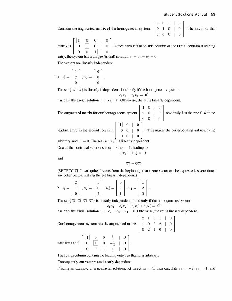
Consider the augmented matrix of the homogeneous system:
⎡⎢⎣ 1 0 1 | 0
0 1 0 | 0
1 0 0 | 0
⎤⎥⎦ . The r.r.e.f. of thismatrix is
⎡⎢⎣ 1 0 0 | 0
0 1 0 | 0
0 0 1 | 0
⎤⎥⎦ . Since each left hand side column of the r.r.e.f. contains a leading
entry, the system has a unique (trivial) solution c1 = c2 = c3 = 0.
The vectors are linearly independent.
3. a. −→u1 =
⎡⎢⎣ 1
2
0
⎤⎥⎦ ,−→u2 =
⎡⎢⎣ 0
0
0
⎤⎥⎦ .The set {−→u1 ,−→u2} is linearly independent if and only if the homogeneous system
c1−→u1 + c2−→u2 =−→0
has only the trivial solution c1 = c2 = 0. Otherwise, the set is linearly dependent.
The augmented matrix for our homogeneous system
⎡⎢⎣ 1 0 | 0
2 0 | 0
0 0 | 0
⎤⎥⎦ obviously has the r.r.e.f. with no
leading entry in the second column (
⎡⎢⎣ 1 0 | 0
0 0 | 0
0 0 | 0
⎤⎥⎦). This makes the corresponding unknown (c2)
arbitrary, and c1 = 0. The set {−→u1 ,−→u2} is linearly dependent.One of the nontrivial solutions is c1 = 0, c2 = 1, leading to
0−→u1 + 1−→u2 =−→0
and−→u2 = 0−→u1
(SHORTCUT: It was quite obvious from the beginning, that a zero vector can be expressed as zero times
any other vector, making the set linearly dependent.)
b. −→u1 =
⎡⎢⎣ 2
1
0
⎤⎥⎦ ,−→u2 =
⎡⎢⎣ 1
0
2
⎤⎥⎦ ,−→u3 =
⎡⎢⎣ 0
2
1
⎤⎥⎦ ,−→u4 =
⎡⎢⎣ 1
2
0
⎤⎥⎦ .The set {−→u1 ,−→u2 ,−→u3 ,−→u4} is linearly independent if and only if the homogeneous system
c1−→u1 + c2−→u2 + c3−→u3 + c4−→u4 =−→0
has only the trivial solution c1 = c2 = c3 = c4 = 0. Otherwise, the set is linearly dependent.
Our homogeneous system has the augmented matrix
⎡⎢⎣ 2 1 0 1 | 0
1 0 2 2 | 0
0 2 1 0 | 0
⎤⎥⎦
with the r.r.e.f.
⎡⎢⎣ 1 0 0 23 | 0
0 1 0 −13
| 0
0 0 1 23 | 0
⎤⎥⎦ .The fourth column contains no leading entry, so that c4 is arbitrary.
Consequently our vectors are linearly dependent.
Finding an example of a nontrivial solution, let us set c4 = 3, then calculate c1 = −2, c2 = 1, and
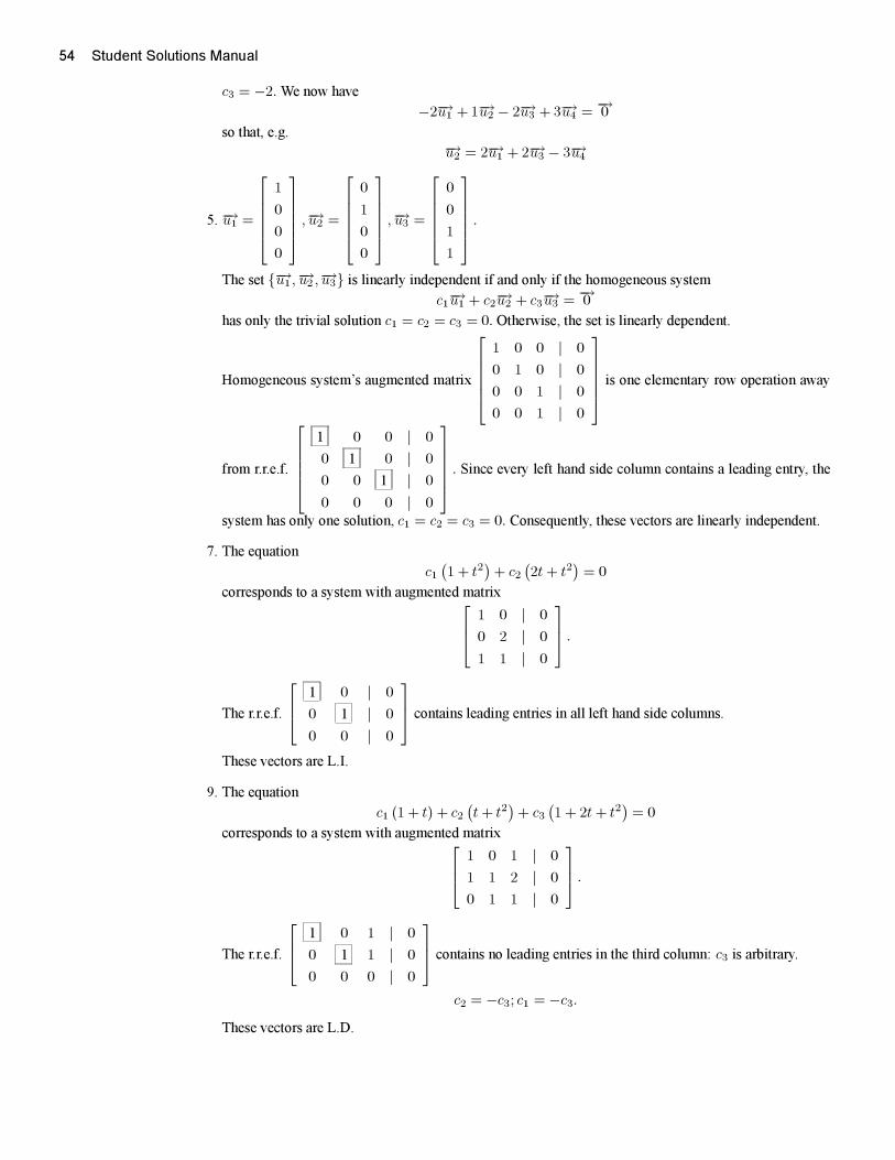
54 Student Solutions Manual
c3 = −2.We now have
−2−→u1 +1−→u2 − 2−→u3 +3−→u4 =−→0
so that, e.g.−→u2 = 2−→u1 +2−→u3 − 3−→u4
5. −→u1 =
⎡⎢⎢⎢⎢⎣1
0
0
0
⎤⎥⎥⎥⎥⎦ ,−→u2 =
⎡⎢⎢⎢⎢⎣0
1
0
0
⎤⎥⎥⎥⎥⎦ ,−→u3 =
⎡⎢⎢⎢⎢⎣0
0
1
1
⎤⎥⎥⎥⎥⎦ .The set {−→u1 ,−→u2 ,−→u3} is linearly independent if and only if the homogeneous system
c1−→u1 + c2−→u2 + c3−→u3 =−→0
has only the trivial solution c1 = c2 = c3 = 0. Otherwise, the set is linearly dependent.
Homogeneous system’s augmented matrix
⎡⎢⎢⎢⎢⎣1 0 0 | 0
0 1 0 | 0
0 0 1 | 0
0 0 1 | 0
⎤⎥⎥⎥⎥⎦ is one elementary row operation away
from r.r.e.f.
⎡⎢⎢⎢⎢⎣1 0 0 | 0
0 1 0 | 0
0 0 1 | 0
0 0 0 | 0
⎤⎥⎥⎥⎥⎦ . Since every left hand side column contains a leading entry, the
system has only one solution, c1 = c2 = c3 = 0. Consequently, these vectors are linearly independent.
7. The equation
c1(1 + t2
)+ c2
(2t+ t2
)= 0
corresponds to a system with augmented matrix⎡⎢⎣ 1 0 | 0
0 2 | 0
1 1 | 0
⎤⎥⎦ .
The r.r.e.f.
⎡⎢⎣ 1 0 | 0
0 1 | 0
0 0 | 0
⎤⎥⎦ contains leading entries in all left hand side columns.
These vectors are L.I.
9. The equation
c1 (1 + t) + c2(t+ t2
)+ c3
(1 + 2t+ t2
)= 0
corresponds to a system with augmented matrix⎡⎢⎣ 1 0 1 | 0
1 1 2 | 0
0 1 1 | 0
⎤⎥⎦ .
The r.r.e.f.
⎡⎢⎣ 1 0 1 | 0
0 1 1 | 0
0 0 0 | 0
⎤⎥⎦ contains no leading entries in the third column: c3 is arbitrary.
c2 = −c3; c1 = −c3.
These vectors are L.D.
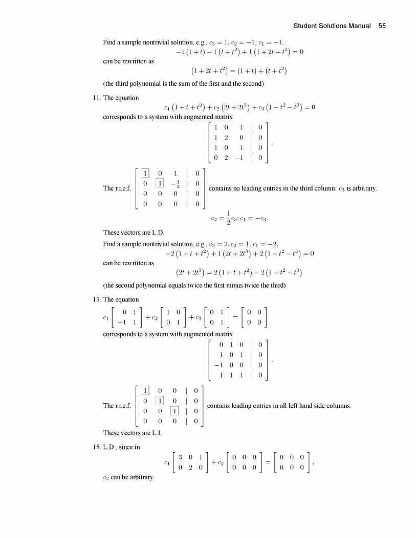
Student Solutions Manual 55
Find a sample nontrivial solution, e.g., c3 = 1, c2 = −1, c1 = −1.
−1 (1 + t) − 1(t+ t2
)+ 1(1 + 2t+ t2
)= 0
can be rewritten as (1 + 2t+ t2
)= (1 + t) +
(t+ t2
)(the third polynomial is the sum of the first and the second)
11. The equation
c1(1 + t + t2
)+ c2
(2t+2t3
)+ c3
(1 + t2 − t3
)= 0
corresponds to a system with augmented matrix⎡⎢⎢⎢⎢⎣1 0 1 | 0
1 2 0 | 0
1 0 1 | 0
0 2 −1 | 0
⎤⎥⎥⎥⎥⎦ .
The r.r.e.f.
⎡⎢⎢⎢⎢⎣1 0 1 | 0
0 1 −12
| 0
0 0 0 | 0
0 0 0 | 0
⎤⎥⎥⎥⎥⎦ contains no leading entries in the third column: c3 is arbitrary.
c2 =1
2c3; c1 = −c3.
These vectors are L.D.
Find a sample nontrivial solution, e.g., c3 = 2, c2 = 1, c1 = −2,
−2(1 + t + t2
)+ 1(2t+ 2t3
)+ 2(1 + t2 − t3
)= 0
can be rewritten as (2t+ 2t3
)= 2(1 + t+ t2
)− 2(1 + t2 − t3
)(the second polynomial equals twice the first minus twice the third)
13. The equation
c1
[0 1
−1 1
]+ c2
[1 0
0 1
]+ c3
[0 1
0 1
]=
[0 0
0 0
]corresponds to a system with augmented matrix⎡⎢⎢⎢⎢⎣
0 1 0 | 0
1 0 1 | 0
−1 0 0 | 0
1 1 1 | 0
⎤⎥⎥⎥⎥⎦ .
The r.r.e.f.
⎡⎢⎢⎢⎢⎣1 0 0 | 0
0 1 0 | 0
0 0 1 | 0
0 0 0 | 0
⎤⎥⎥⎥⎥⎦ contains leading entries in all left hand side columns.
These vectors are L.I.
15. L.D., since in
c1
[3 0 1
0 2 0
]+ c2
[0 0 0
0 0 0
]=
[0 0 0
0 0 0
],
c2 can be arbitrary.
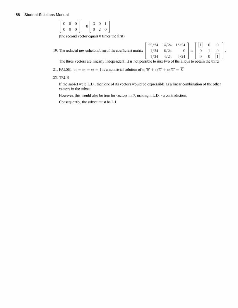
56 Student Solutions Manual[0 0 0
0 0 0
]= 0
[3 0 1
0 2 0
](the second vector equals 0 times the first)
19. The reduced row echelon form of the coefficient matrix
⎡⎢⎣ 22/24 14/24 18/24
1/24 6/24 0
1/24 4/24 6/24
⎤⎥⎦ is⎡⎢⎣ 1 0 0
0 1 0
0 0 1
⎤⎥⎦ .The three vectors are linearly independent. It is not possible to mix two of the alloys to obtain the third.
21. FALSE: c1 = c2 = c3 = 1 is a nontrivial solution of c1−→u + c2−→v + c3−→w =−→0
23. TRUE
If the subset were L.D., then one of its vectors would be expressible as a linear combination of the other
vectors in the subset.
However, this would also be true for vectors in S, making it L.D. - a contradiction.
Consequently, the subset must be L.I.

Student Solutions Manual 57
Section
4.41. The number of vectors in the set, 2, matches dimR2. Therefore, by Theorem 4.16, it is sufficient to show
that the set is L.I.
The resulting homogeneous system has the augmented matrix
[2 −1 | 0
1 3 | 0
]with the r.r.e.f.
[1 0 | 0
0 1 | 0
]. There is a leading entry in each left hand side column, making the solution unique.
The set is L.I., therefore, (by Theorem 4.16) it is also a basis forR2.
3. The number of vectors in the set, 3, does not match dimR2 = 2. The set cannot be a basis forR2.
5. The number of vectors in the set, 2, does not match dimR3 = 3. The set cannot be a basis forR3.
7. The number of vectors in the set, 3, matches dimR3. Therefore, by Theorem 4.16, it is sufficient to show
that the set is L.I.
The resulting homogeneous system has the augmented matrix
⎡⎢⎣ 1 0 −1 | 0
0 1 1 | 0
1 1 0 | 0
⎤⎥⎦ with the r.r.e.f.
⎡⎢⎣ 1 0 −1 | 0
0 1 1 | 0
0 0 0 | 0
⎤⎥⎦ . There are many solutions, including some nontrivial ones, making the set
L.D. Therefore, it is not a basis for R3.
9. The number of vectors in the set, 4, matches dimR4. Therefore, by Theorem 4.16, it is sufficient to show
that the set is L.I.
The resulting homogeneous system has the augmented matrix
⎡⎢⎢⎢⎢⎣1 0 0 0 | 0
0 0 1 0 | 0
0 1 0 0 | 0
1 0 1 1 | 0
⎤⎥⎥⎥⎥⎦ with the r.r.e.f.
⎡⎢⎢⎢⎢⎣1 0 0 0 | 0
0 1 0 0 | 0
0 0 1 0 | 0
0 0 0 1 | 0
⎤⎥⎥⎥⎥⎦ . There is a leading entry in each left hand side column, making the
solution unique. The set is L.I., therefore, (by Theorem 4.16) it is also a basis forR4.
11. The number of vectors in the set, 2, does not match dimP2 = 3. The set cannot be a basis for P2.
13. The number of vectors in the set, 2, matches dimP1. Therefore, by Theorem 4.16, it is sufficient to show
that the set is L.I.
The equation
c1 (2 + t) + c2(1 + 3t) = 0
corresponds to the homogeneous system with the augmented matrix
[2 1 | 0
1 3 | 0
]. The r.r.e.f. is[
1 0 | 0
0 1 | 0
]. There is a leading entry in each left hand side column, making the solution unique.
The set is L.I., therefore, (by Theorem 4.16) it is also a basis for P1.
15. The number of vectors in the set, 3, does not match dimP3 = 4. The set cannot be a basis for P3.
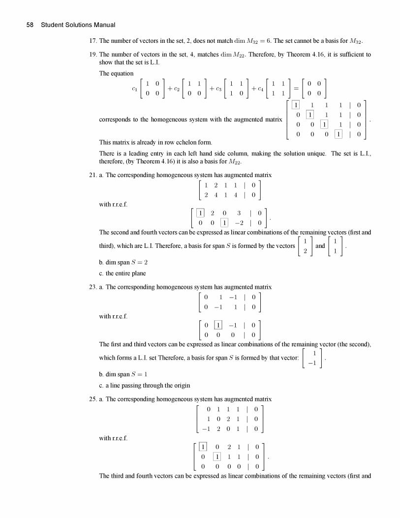
58 Student Solutions Manual
17. The number of vectors in the set, 2, does not match dimM32 = 6. The set cannot be a basis forM32.
19. The number of vectors in the set, 4, matches dimM22. Therefore, by Theorem 4.16, it is sufficient to
show that the set is L.I.
The equation
c1
[1 0
0 0
]+ c2
[1 1
0 0
]+ c3
[1 1
1 0
]+ c4
[1 1
1 1
]=
[0 0
0 0
]
corresponds to the homogeneous system with the augmented matrix
⎡⎢⎢⎢⎢⎣1 1 1 1 | 0
0 1 1 1 | 0
0 0 1 1 | 0
0 0 0 1 | 0
⎤⎥⎥⎥⎥⎦ .This matrix is already in row echelon form.
There is a leading entry in each left hand side column, making the solution unique. The set is L.I.,
therefore, (by Theorem 4.16) it is also a basis forM22.
21. a. The corresponding homogeneous system has augmented matrix[1 2 1 1 | 0
2 4 1 4 | 0
]with r.r.e.f. [
1 2 0 3 | 0
0 0 1 −2 | 0
].
The second and fourth vectors can be expressed as linear combinations of the remaining vectors (first and
third), which are L.I. Therefore, a basis for span S is formed by the vectors
[1
2
]and
[1
1
].
b. dim span S = 2
c. the entire plane
23. a. The corresponding homogeneous system has augmented matrix[0 1 −1 | 0
0 −1 1 | 0
]with r.r.e.f. [
0 1 −1 | 0
0 0 0 | 0
]The first and third vectors can be expressed as linear combinations of the remaining vector (the second),
which forms a L.I. set Therefore, a basis for span S is formed by that vector:
[1
−1
].
b. dim span S = 1
c. a line passing through the origin
25. a. The corresponding homogeneous system has augmented matrix⎡⎢⎣ 0 1 1 1 | 0
1 0 2 1 | 0
−1 2 0 1 | 0
⎤⎥⎦with r.r.e.f. ⎡⎢⎣ 1 0 2 1 | 0
0 1 1 1 | 0
0 0 0 0 | 0
⎤⎥⎦ .The third and fourth vectors can be expressed as linear combinations of the remaining vectors (first and
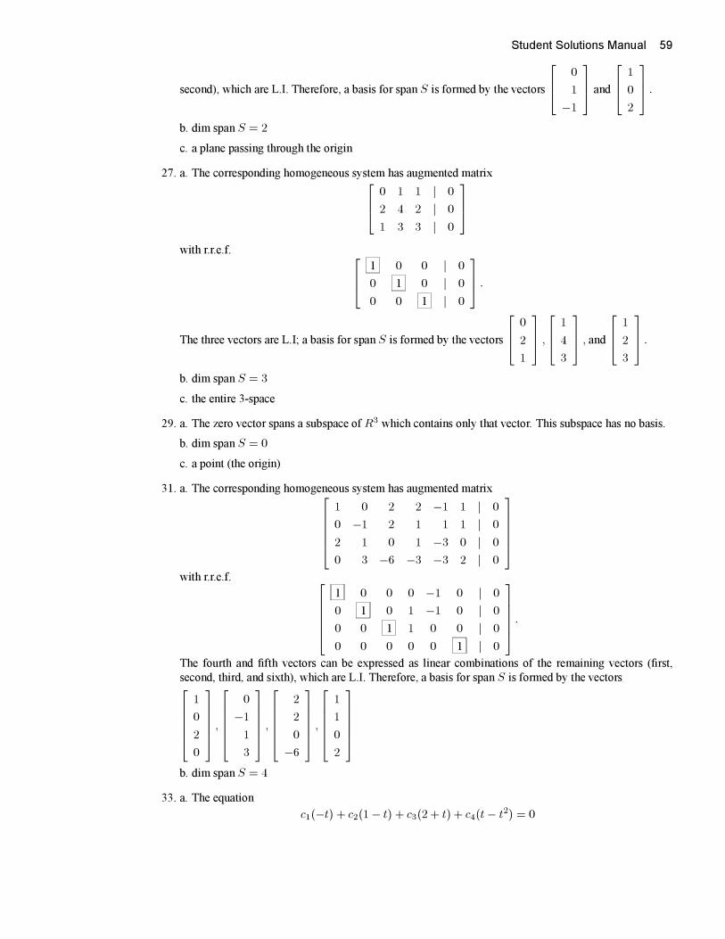
Student Solutions Manual 59
second), which are L.I. Therefore, a basis for span S is formed by the vectors
⎡⎢⎣ 0
1
−1
⎤⎥⎦ and
⎡⎢⎣ 1
0
2
⎤⎥⎦ .b. dim span S = 2
c. a plane passing through the origin
27. a. The corresponding homogeneous system has augmented matrix⎡⎢⎣ 0 1 1 | 0
2 4 2 | 0
1 3 3 | 0
⎤⎥⎦with r.r.e.f. ⎡⎢⎣ 1 0 0 | 0
0 1 0 | 0
0 0 1 | 0
⎤⎥⎦ .
The three vectors are L.I; a basis for span S is formed by the vectors
⎡⎢⎣ 0
2
1
⎤⎥⎦ ,⎡⎢⎣ 1
4
3
⎤⎥⎦ , and⎡⎢⎣ 1
2
3
⎤⎥⎦ .b. dim span S = 3
c. the entire 3-space
29. a. The zero vector spans a subspace of R3 which contains only that vector. This subspace has no basis.
b. dim span S = 0
c. a point (the origin)
31. a. The corresponding homogeneous system has augmented matrix⎡⎢⎢⎢⎢⎣1 0 2 2 −1 1 | 0
0 −1 2 1 1 1 | 0
2 1 0 1 −3 0 | 0
0 3 −6 −3 −3 2 | 0
⎤⎥⎥⎥⎥⎦with r.r.e.f. ⎡⎢⎢⎢⎢⎣
1 0 0 0 −1 0 | 0
0 1 0 1 −1 0 | 0
0 0 1 1 0 0 | 0
0 0 0 0 0 1 | 0
⎤⎥⎥⎥⎥⎦ .The fourth and fifth vectors can be expressed as linear combinations of the remaining vectors (first,
second, third, and sixth), which are L.I. Therefore, a basis for span S is formed by the vectors⎡⎢⎢⎢⎢⎣1
0
2
0
⎤⎥⎥⎥⎥⎦ ,⎡⎢⎢⎢⎢⎣
0
−1
1
3
⎤⎥⎥⎥⎥⎦ ,⎡⎢⎢⎢⎢⎣
2
2
0
−6
⎤⎥⎥⎥⎥⎦ ,⎡⎢⎢⎢⎢⎣
1
1
0
2
⎤⎥⎥⎥⎥⎦b. dim span S = 4
33. a. The equation
c1(−t) + c2(1− t) + c3(2 + t) + c4(t− t2) = 0
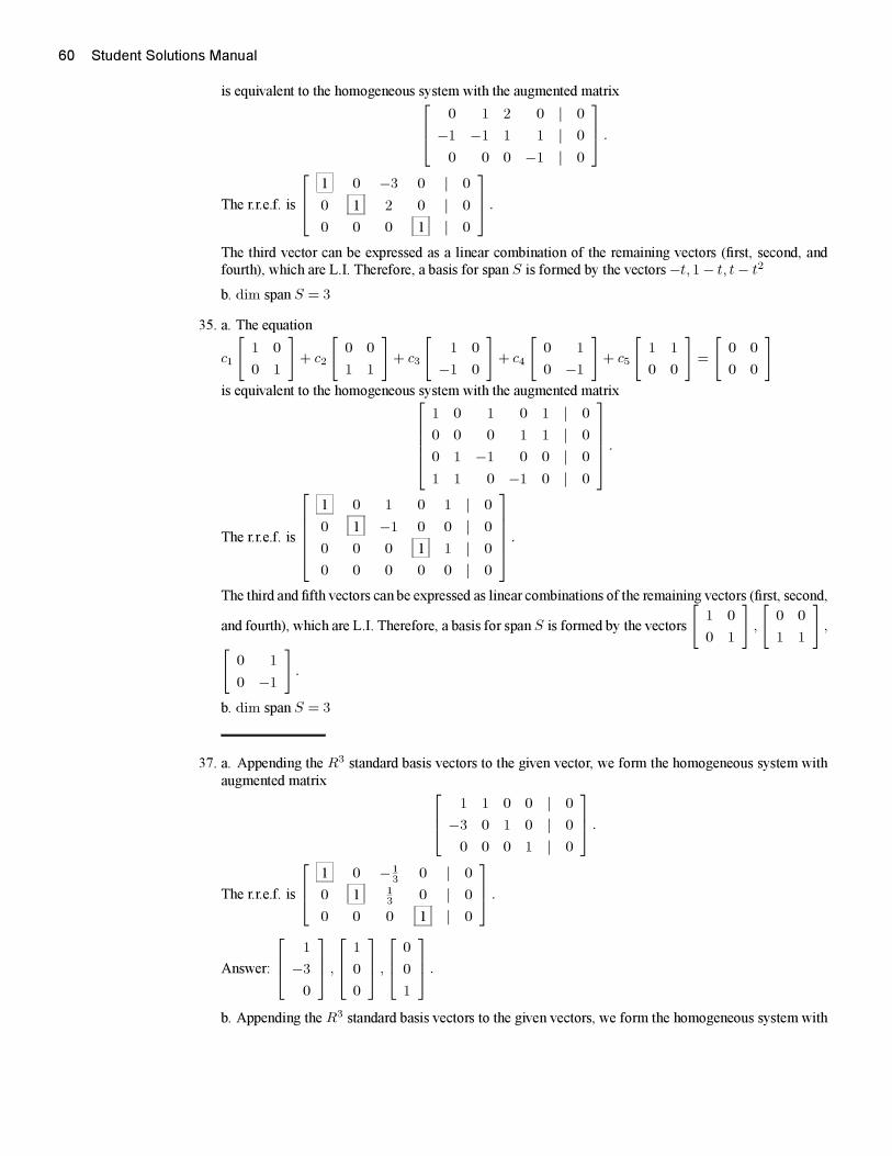
60 Student Solutions Manual
is equivalent to the homogeneous system with the augmented matrix⎡⎢⎣ 0 1 2 0 | 0
−1 −1 1 1 | 0
0 0 0 −1 | 0
⎤⎥⎦ .
The r.r.e.f. is
⎡⎢⎣ 1 0 −3 0 | 0
0 1 2 0 | 0
0 0 0 1 | 0
⎤⎥⎦ .The third vector can be expressed as a linear combination of the remaining vectors (first, second, and
fourth), which are L.I. Therefore, a basis for span S is formed by the vectors−t, 1− t, t− t2
b. dim span S = 3
35. a. The equation
c1
[1 0
0 1
]+ c2
[0 0
1 1
]+ c3
[1 0
−1 0
]+ c4
[0 1
0 −1
]+ c5
[1 1
0 0
]=
[0 0
0 0
]is equivalent to the homogeneous system with the augmented matrix⎡⎢⎢⎢⎢⎣
1 0 1 0 1 | 0
0 0 0 1 1 | 0
0 1 −1 0 0 | 0
1 1 0 −1 0 | 0
⎤⎥⎥⎥⎥⎦ .
The r.r.e.f. is
⎡⎢⎢⎢⎢⎣1 0 1 0 1 | 0
0 1 −1 0 0 | 0
0 0 0 1 1 | 0
0 0 0 0 0 | 0
⎤⎥⎥⎥⎥⎦ .The third and fifth vectors can be expressed as linear combinations of the remaining vectors (first, second,
and fourth), which are L.I. Therefore, a basis for spanS is formed by the vectors
[1 0
0 1
],
[0 0
1 1
],[
0 1
0 −1
].
b. dim span S = 3
37. a. Appending the R3 standard basis vectors to the given vector, we form the homogeneous system with
augmented matrix ⎡⎢⎣ 1 1 0 0 | 0
−3 0 1 0 | 0
0 0 0 1 | 0
⎤⎥⎦ .
The r.r.e.f. is
⎡⎢⎣ 1 0 −13 0 | 0
0 1 13 0 | 0
0 0 0 1 | 0
⎤⎥⎦ .
Answer:
⎡⎢⎣ 1
−3
0
⎤⎥⎦ ,⎡⎢⎣ 1
0
0
⎤⎥⎦ ,⎡⎢⎣ 0
0
1
⎤⎥⎦ .b. Appending the R3 standard basis vectors to the given vectors, we form the homogeneous system with
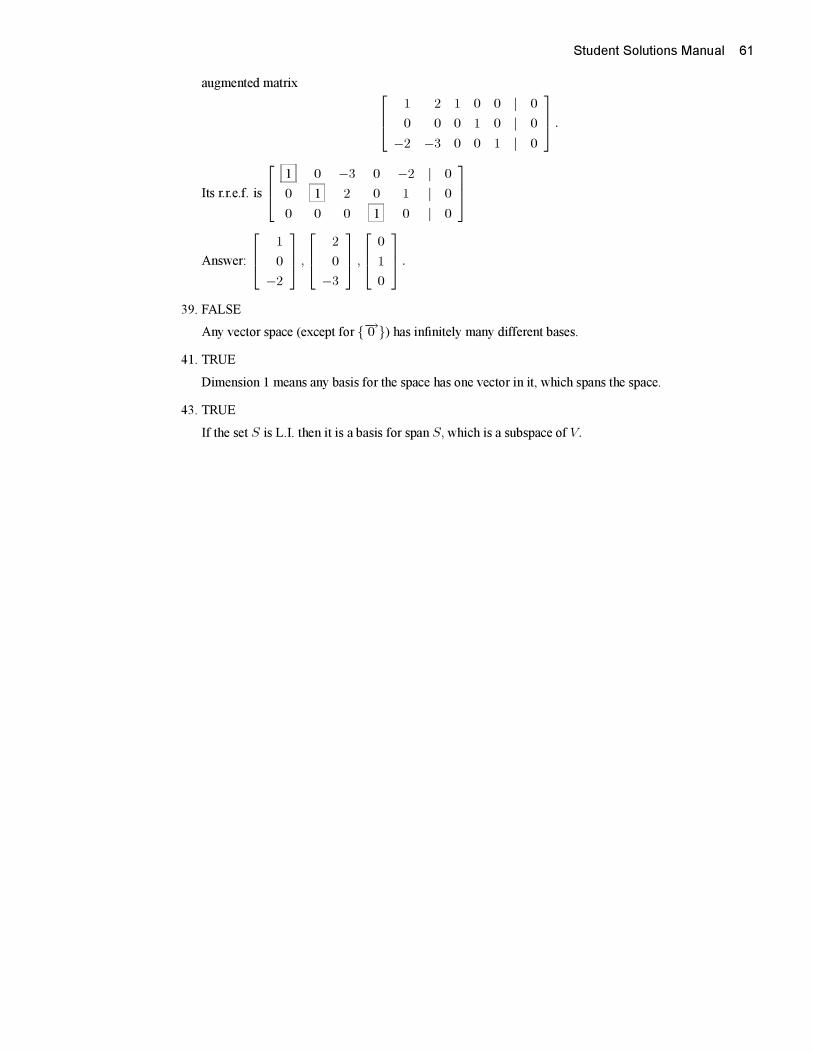
Student Solutions Manual 61
augmented matrix ⎡⎢⎣ 1 2 1 0 0 | 0
0 0 0 1 0 | 0
−2 −3 0 0 1 | 0
⎤⎥⎦ .
Its r.r.e.f. is
⎡⎢⎣ 1 0 −3 0 −2 | 0
0 1 2 0 1 | 0
0 0 0 1 0 | 0
⎤⎥⎦
Answer:
⎡⎢⎣ 1
0
−2
⎤⎥⎦ ,⎡⎢⎣ 2
0
−3
⎤⎥⎦ ,⎡⎢⎣ 0
1
0
⎤⎥⎦ .39. FALSE
Any vector space (except for {−→0 }) has infinitely many different bases.
41. TRUE
Dimension 1 means any basis for the space has one vector in it, which spans the space.
43. TRUE
If the set S is L.I. then it is a basis for span S, which is a subspace of V.
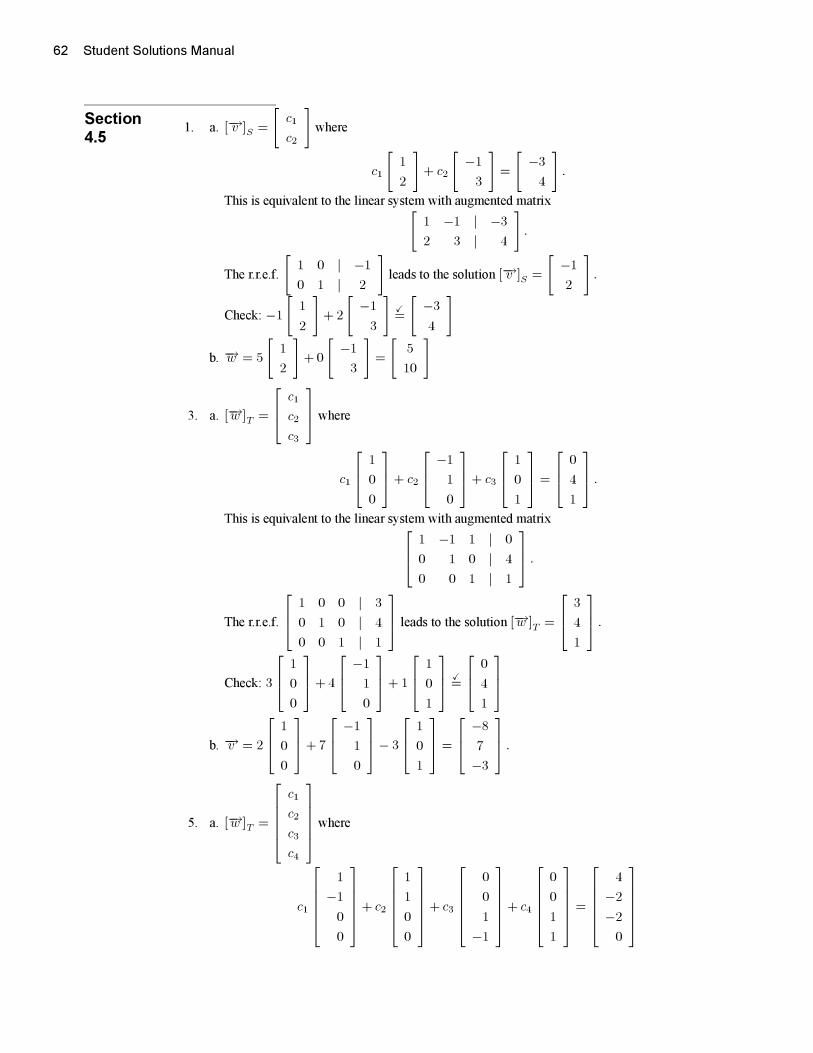
62 Student Solutions Manual
Section
4.51. a. [−→v ]S =
[c1
c2
]where
c1
[1
2
]+ c2
[−1
3
]=
[−3
4
].
This is equivalent to the linear system with augmented matrix[1 −1 | −3
2 3 | 4
].
The r.r.e.f.
[1 0 | −1
0 1 | 2
]leads to the solution [−→v ]S =
[−1
2
].
Check: −1
[1
2
]+ 2
[−1
3
]�=
[−3
4
]
b. −→w = 5
[1
2
]+0
[−1
3
]=
[5
10
]
3. a. [−→w ]T =
⎡⎢⎣ c1
c2
c3
⎤⎥⎦ where
c1
⎡⎢⎣ 1
0
0
⎤⎥⎦+ c2
⎡⎢⎣ −1
1
0
⎤⎥⎦+ c3
⎡⎢⎣ 1
0
1
⎤⎥⎦ =
⎡⎢⎣ 0
4
1
⎤⎥⎦ .This is equivalent to the linear system with augmented matrix⎡⎢⎣ 1 −1 1 | 0
0 1 0 | 4
0 0 1 | 1
⎤⎥⎦ .
The r.r.e.f.
⎡⎢⎣ 1 0 0 | 3
0 1 0 | 4
0 0 1 | 1
⎤⎥⎦ leads to the solution [−→w ]T =
⎡⎢⎣ 3
4
1
⎤⎥⎦ .Check: 3
⎡⎢⎣ 1
0
0
⎤⎥⎦+4
⎡⎢⎣ −1
1
0
⎤⎥⎦+ 1
⎡⎢⎣ 1
0
1
⎤⎥⎦ �=
⎡⎢⎣ 0
4
1
⎤⎥⎦b. −→v = 2
⎡⎢⎣ 1
0
0
⎤⎥⎦+7
⎡⎢⎣ −1
1
0
⎤⎥⎦− 3
⎡⎢⎣ 1
0
1
⎤⎥⎦ =
⎡⎢⎣ −8
7
−3
⎤⎥⎦ .
5. a. [−→w ]T =
⎡⎢⎢⎢⎢⎣c1
c2
c3
c4
⎤⎥⎥⎥⎥⎦ where
c1
⎡⎢⎢⎢⎢⎣1
−1
0
0
⎤⎥⎥⎥⎥⎦+ c2
⎡⎢⎢⎢⎢⎣1
1
0
0
⎤⎥⎥⎥⎥⎦+ c3
⎡⎢⎢⎢⎢⎣0
0
1
−1
⎤⎥⎥⎥⎥⎦+ c4
⎡⎢⎢⎢⎢⎣0
0
1
1
⎤⎥⎥⎥⎥⎦ =
⎡⎢⎢⎢⎢⎣4
−2
−2
0
⎤⎥⎥⎥⎥⎦
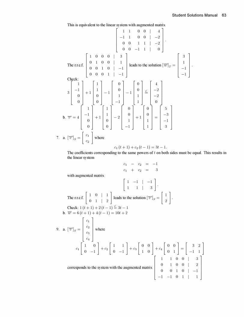
Student Solutions Manual 63
This is equivalent to the linear system with augmented matrix⎡⎢⎢⎢⎢⎣1 1 0 0 | 4
−1 1 0 0 | −2
0 0 1 1 | −2
0 0 −1 1 | 0
⎤⎥⎥⎥⎥⎦ .
The r.r.e.f.
⎡⎢⎢⎢⎢⎣1 0 0 0 | 3
0 1 0 0 | 1
0 0 1 0 | −1
0 0 0 1 | −1
⎤⎥⎥⎥⎥⎦ leads to the solution [−→w ]T =
⎡⎢⎢⎢⎢⎣3
1
−1
−1
⎤⎥⎥⎥⎥⎦ .Check:
3
⎡⎢⎢⎢⎢⎣1
−1
0
0
⎤⎥⎥⎥⎥⎦+1
⎡⎢⎢⎢⎢⎣1
1
0
0
⎤⎥⎥⎥⎥⎦− 1
⎡⎢⎢⎢⎢⎣0
0
1
−1
⎤⎥⎥⎥⎥⎦− 1
⎡⎢⎢⎢⎢⎣0
0
1
1
⎤⎥⎥⎥⎥⎦ �=
⎡⎢⎢⎢⎢⎣4
−2
−2
0
⎤⎥⎥⎥⎥⎦
b. −→v = 4
⎡⎢⎢⎢⎢⎣1
−1
0
0
⎤⎥⎥⎥⎥⎦+ 1
⎡⎢⎢⎢⎢⎣1
1
0
0
⎤⎥⎥⎥⎥⎦− 2
⎡⎢⎢⎢⎢⎣0
0
1
−1
⎤⎥⎥⎥⎥⎦+ 1
⎡⎢⎢⎢⎢⎣0
0
1
1
⎤⎥⎥⎥⎥⎦ =
⎡⎢⎢⎢⎢⎣5
−3
−1
3
⎤⎥⎥⎥⎥⎦7. a. [−→v ]S =
[c1
c2
]where
c1 (t+ 1) + c2 (t− 1) = 3t− 1.
The coefficients corresponding to the same powers of t on both sides must be equal. This results in
the linear system
c1 − c2 = −1
c1 + c2 = 3
with augmented matrix [1 −1 | −1
1 1 | 3
].
The r.r.e.f.
[1 0 | 1
0 1 | 2
]leads to the solution [−→v ]S =
[1
2
].
Check: 1 (t+ 1) + 2 (t− 1)�= 3t− 1
b. −→w = 6 (t+ 1) + 4 (t− 1) = 10t+2
9. a. [−→v ]S =
⎡⎢⎢⎢⎢⎣c1
c2
c3
c4
⎤⎥⎥⎥⎥⎦ where
c1
[1 0
0 −1
]+ c2
[1 1
0 −1
]+ c3
[0 0
1 0
]+ c4
[0 0
0 1
]=
[3 2
−1 1
]
corresponds to the system with the augmented matrix
⎡⎢⎢⎢⎢⎣1 1 0 0 | 3
0 1 0 0 | 2
0 0 1 0 | −1
−1 −1 0 1 | 1
⎤⎥⎥⎥⎥⎦
64 Student Solutions Manual
The r.r.e.f.
⎡⎢⎢⎢⎢⎣1 0 0 0 | 1
0 1 0 0 | 2
0 0 1 0 | −1
0 0 0 1 | 4
⎤⎥⎥⎥⎥⎦ leads to the solution [−→v ]S =
⎡⎢⎢⎢⎢⎣1
2
−1
4
⎤⎥⎥⎥⎥⎦ .Check:
1
[1 0
0 −1
]+2
[1 1
0 −1
]− 1
[0 0
1 0
]+4
[0 0
0 1
]�=
[3 2
−1 1
]
b. −→w = −2
[1 0
0 −1
]+1
[1 1
0 −1
]+ 0
[0 0
1 0
]+0
[0 0
0 1
]=
[−1 1
0 1
]
11. Consider a basis S =
⎧⎪⎨⎪⎩⎡⎢⎣ 1
2
−1
⎤⎥⎦ ,⎡⎢⎣ 0
2
3
⎤⎥⎦⎫⎪⎬⎪⎭ for a 2-dimensional subspace of R3 (a plane passing through
the origin),
a. if possible, find [−→u ]S for −→u =
⎡⎢⎣ 2
−2
−11
⎤⎥⎦⎡⎢⎣ 1 0 2
2 2 −2
−1 3 −11
⎤⎥⎦ has r.r.e.f.
⎡⎢⎣ 1 0 2
0 1 −3
0 0 0
⎤⎥⎦ =⇒ [−→u ]S =
[2
−3
]
and [−→v ]S such that −→v =
⎡⎢⎣ 3
1
1
⎤⎥⎦ ;⎡⎢⎣ 1 0 3
2 2 1
−1 3 1
⎤⎥⎦ has r.r.e.f.
⎡⎢⎣ 1 0 0
0 1 0
0 0 1
⎤⎥⎦ =⇒ [−→v ]S cannot be found
what does it say about a vector when its coordinate vector with respect to S cannot be found?
Answer: such a vector (e.g.,−→v ) is not in the plane spanned by S.
b. find −→w such that [−→w ]S =
[4
1
].
4
⎡⎢⎣ 1
2
−1
⎤⎥⎦+1
⎡⎢⎣ 0
2
3
⎤⎥⎦ =
⎡⎢⎣ 4
10
−1
⎤⎥⎦
Student Solutions Manual 65
Section
4.6 1. a. A row echelon form is
[1 0 2
0 1 3
].
i A basis for the column space:
[1
2
],
[0
−1
].
ii A basis for the row space:
⎡⎢⎣ 1
0
2
⎤⎥⎦ ,⎡⎢⎣ 0
1
3
⎤⎥⎦ .iii 2
iv x3 is arbitrary; x1 = −2x3; x2 = −3x3.⎡⎢⎣ x1
x2
x3
⎤⎥⎦ =
⎡⎢⎣ −2x3
−3x3
x3
⎤⎥⎦ = x3
⎡⎢⎣ −2
−3
1
⎤⎥⎦ .Basis for null space of A :
⎡⎢⎣ −2
−3
1
⎤⎥⎦v 1.
b. A r.e.f.
[1 −2
0 0
]
i A basis for the column space:
[2
−1
].
ii A basis for the row space:
[1
−2
].
iii 1
iv x2 is arbitrary; x1 = 2x2[x1
x2
]=
[2x2
x2
]= x2
[2
1
]
Basis for null space:
[2
1
]v 1.
c. R.e.f. is
⎡⎢⎣ 1 0 −1 2
0 0 0 0
0 0 0 0
⎤⎥⎦ .i A basis for the column space:
⎡⎢⎣ 1
−2
1
⎤⎥⎦
ii A basis for the row space:
⎡⎢⎢⎢⎢⎣1
0
−1
2
⎤⎥⎥⎥⎥⎦iii 1
iv x2, x3, and x4 are arbitrary; x1 = x3 − 2x4.
66 Student Solutions Manual⎡⎢⎢⎢⎢⎣x1
x2
x3
x4
⎤⎥⎥⎥⎥⎦ =
⎡⎢⎢⎢⎢⎣x3 − 2x4
x2
x3
x4
⎤⎥⎥⎥⎥⎦ = x2
⎡⎢⎢⎢⎢⎣0
1
0
0
⎤⎥⎥⎥⎥⎦+ x3
⎡⎢⎢⎢⎢⎣1
0
1
0
⎤⎥⎥⎥⎥⎦+ x4
⎡⎢⎢⎢⎢⎣−2
0
0
1
⎤⎥⎥⎥⎥⎦
Basis for null space of A :
⎡⎢⎢⎢⎢⎣0
1
0
0
⎤⎥⎥⎥⎥⎦ ,⎡⎢⎢⎢⎢⎣
1
0
1
0
⎤⎥⎥⎥⎥⎦ ,⎡⎢⎢⎢⎢⎣
−2
0
0
1
⎤⎥⎥⎥⎥⎦v 3.
3. a. R.e.f. is
⎡⎢⎢⎢⎢⎣1 0 −1
0 1 0
0 0 1
0 0 0
⎤⎥⎥⎥⎥⎦ .
i A basis for the column space: .
⎡⎢⎢⎢⎢⎣1
0
0
1
⎤⎥⎥⎥⎥⎦ ,⎡⎢⎢⎢⎢⎣
0
2
1
0
⎤⎥⎥⎥⎥⎦ ,⎡⎢⎢⎢⎢⎣
−1
0
3
1
⎤⎥⎥⎥⎥⎦ii A basis for the row space:
⎡⎢⎣ 1
0
−1
⎤⎥⎦ ,⎡⎢⎣ 0
1
0
⎤⎥⎦ ,⎡⎢⎣ 0
0
1
⎤⎥⎦iii 3
iv The only solution is
⎡⎢⎣ 0
0
0
⎤⎥⎦ .No basis for null space of A.
v 0.
b. The r.e.f. is
⎡⎢⎢⎢⎢⎣0 1 −1 0 0 2
0 0 1 0 1 −1
0 0 0 1 1 −1
0 0 0 0 0 0
⎤⎥⎥⎥⎥⎦ .
i A basis for the column space:
⎡⎢⎢⎢⎢⎣0
1
0
1
⎤⎥⎥⎥⎥⎦ ,⎡⎢⎢⎢⎢⎣
0
−1
0
1
⎤⎥⎥⎥⎥⎦ ,⎡⎢⎢⎢⎢⎣
1
0
2
0
⎤⎥⎥⎥⎥⎦
ii A basis for the row space:
⎡⎢⎢⎢⎢⎢⎢⎢⎢⎢⎣
0
1
−1
0
0
2
⎤⎥⎥⎥⎥⎥⎥⎥⎥⎥⎦,
⎡⎢⎢⎢⎢⎢⎢⎢⎢⎢⎣
0
0
1
0
1
−1
⎤⎥⎥⎥⎥⎥⎥⎥⎥⎥⎦,
⎡⎢⎢⎢⎢⎢⎢⎢⎢⎢⎣
0
0
0
1
1
−1
⎤⎥⎥⎥⎥⎥⎥⎥⎥⎥⎦iii 3
iv The r.r.e.f. is
⎡⎢⎢⎢⎢⎣0 1 0 0 1 1
0 0 1 0 1 −1
0 0 0 1 1 −1
0 0 0 0 0 0
⎤⎥⎥⎥⎥⎦
Student Solutions Manual 67
x1, x5, and x6 are arbitrary; x2 = −x5 − x6; x3 = −x5 + x6; x4 = −x5 + x6⎡⎢⎢⎢⎢⎢⎢⎢⎢⎢⎣
x1
x2
x3
x4
x5
x6
⎤⎥⎥⎥⎥⎥⎥⎥⎥⎥⎦=
⎡⎢⎢⎢⎢⎢⎢⎢⎢⎢⎣
x1
−x5 − x6
−x5 + x6
−x5 + x6
x5
x6
⎤⎥⎥⎥⎥⎥⎥⎥⎥⎥⎦= x1
⎡⎢⎢⎢⎢⎢⎢⎢⎢⎢⎣
1
0
0
0
0
0
⎤⎥⎥⎥⎥⎥⎥⎥⎥⎥⎦+ x5
⎡⎢⎢⎢⎢⎢⎢⎢⎢⎢⎣
0
−1
−1
−1
1
0
⎤⎥⎥⎥⎥⎥⎥⎥⎥⎥⎦+ x6
⎡⎢⎢⎢⎢⎢⎢⎢⎢⎢⎣
0
−1
1
1
0
1
⎤⎥⎥⎥⎥⎥⎥⎥⎥⎥⎦
Basis for null space of A :
⎡⎢⎢⎢⎢⎢⎢⎢⎢⎢⎣
1
0
0
0
0
0
⎤⎥⎥⎥⎥⎥⎥⎥⎥⎥⎦,
⎡⎢⎢⎢⎢⎢⎢⎢⎢⎢⎣
0
−1
−1
−1
1
0
⎤⎥⎥⎥⎥⎥⎥⎥⎥⎥⎦,
⎡⎢⎢⎢⎢⎢⎢⎢⎢⎢⎣
0
−1
1
1
0
1
⎤⎥⎥⎥⎥⎥⎥⎥⎥⎥⎦v 3.
5. a. rank [A | −→b ] = rank A+1 (the discrepancy corresponds to the row [0...0|nonzero] )b. rank [A |−→b ] = rank A = n (no row [0...0|nonzero]; every one of the n left hand side columns
contains a leading entry)
c. rank [A |−→b ] = rank A < n (no row [0...0|nonzero]; at least one of the left hand side columns does
not contain a leading entry)
7. TRUE
9. TRUE
There are 7 columns inR4 - no more than 4 vectors can be L.I. inR4.
11. e.g.,
⎡⎢⎣ 1 0 0 0 0 0
0 1 0 0 0 0
0 0 0 0 0 0
⎤⎥⎦13. Such matrix cannot exist -
rank+nullity=3, therefore, both must be no bigger than 3
17. Consider anm× n matrix A and an n × p matrix B.
a. If −→x ∈ (null space of B) then B−→x =−→0 . Therefore, AB−→x = A
−→0 =
−→0 , which implies−→x ∈ (null space of AB).
b. e.g., −→x =
⎡⎢⎣ 0
1
0
⎤⎥⎦ ∈ (null space of AB) but B−→x =
⎡⎢⎣ 1 0 0
0 1 0
0 0 0
⎤⎥⎦⎡⎢⎣ 0
1
0
⎤⎥⎦ =
⎡⎢⎣ 0
1
0
⎤⎥⎦ �= −→0 so that
−→x /∈ (null space of B).
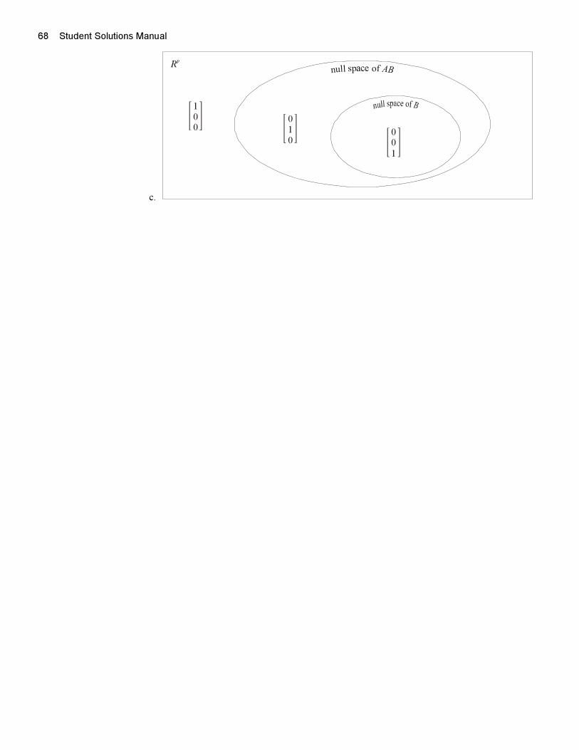
68 Student Solutions Manual
c.
null space of ABR
p
0
0
1
1
0
00
1
0
Student Solutions Manual 69
Section
5.11. For each F : R2 → R2 decide if F is a linear transformation:
a. F (
[x
y
]) =
[2x
3x
];
Yes
Cond. 1 LHS = F (
[x
y
]+
[x′
y′
]) = F (
[x+ x′
y + y′
]) =
[2(x+ x′)3(x+ x′)
]
RHS = F (
[x
y
]) + F (
[x′
y′
]) =
[2x
3x
]+
[2x′
3x′
]√
Cond. 2 LHS = F (c
[x
y
]) = F (
[cx
cy
]) =
[2cx
3cx
]
RHS = cF (
[x
y
]) = c
[2x
3x
]√
b. F (
[x
y
]) =
[0
x− y
];
Yes.
Cond. 1 LHS = F (
[x
y
]+
[x′
y′
]) = F (
[x+ x′
y + y′
]) =
[0
x+ x′ − (y + y′)
]
RHS = F (
[x
y
]) + F (
[x′
y′
]) =
[0
x− y
]+
[0
x′ − y′
]√
Cond. 2 LHS = F (c
[x
y
]) = F (
[cx
cy
]) =
[0
cx− cy
]
RHS = cF (
[x
y
]) = c
[0
x− y
]√
c. F (
[x
y
]) =
[2
−y
].
No.
e.g., Condition 2 does not hold for
LHS = F (2
[0
0
]) = F (
[0
0
]) =
[2
0
]
RHS = 2F (
[0
0
]) = 2
[2
0
]=
[4
0
]not equal
3. For each F : R3 → R2 decide if F is a linear transformation:
a. F (
⎡⎢⎣ x
y
z
⎤⎥⎦) = [ x
yz
];
No.
e.g. Condition 2 does not hold for
70 Student Solutions Manual
LHS = F (2
⎡⎢⎣ 1
2
3
⎤⎥⎦) = F (
⎡⎢⎣ 2
4
6
⎤⎥⎦) = [ 2
24
]
RHS = 2F (
⎡⎢⎣ 1
2
3
⎤⎥⎦) = 2
[1
6
]=
[2
12
]not equal
b. F (
⎡⎢⎣ x
y
z
⎤⎥⎦) = [ y
2z
];
Yes.
Cond. 1 LHS = F (
⎡⎢⎣ x
y
z
⎤⎥⎦+
⎡⎢⎣ x′
y′
z′
⎤⎥⎦) = F (
⎡⎢⎣ x+ x′
y + y′
z + z′
⎤⎥⎦) = [ y + y′
2(z + z′)
]
RHS = F (
⎡⎢⎣ x
y
z
⎤⎥⎦) + F (
⎡⎢⎣ x′
y′
z′
⎤⎥⎦) = [ y
2z
]+
[y′
2z′
]√
Cond. 2 LHS = F (c
⎡⎢⎣ x
y
z
⎤⎥⎦) = F (
⎡⎢⎣ cx
cy
cz
⎤⎥⎦) = [ cy
2cz
]
RHS = cF (
⎡⎢⎣ x
y
z
⎤⎥⎦) = c
[y
2z
]√
c. F (
⎡⎢⎣ x
y
z
⎤⎥⎦) = [ x+ 2z
3y − 2
].
No.
e.g. Condition 1 does not hold for
LHS = F (
⎡⎢⎣ 0
0
0
⎤⎥⎦+
⎡⎢⎣ 1
1
1
⎤⎥⎦) = F (
⎡⎢⎣ 1
1
1
⎤⎥⎦) = [ 3
1
]
RHS = F (
⎡⎢⎣ 0
0
0
⎤⎥⎦) + F (
⎡⎢⎣ 1
1
1
⎤⎥⎦) = [ 0
−2
]+
[3
1
]=
[3
−1
]not equal
5. For eachG : R2 → R decide if G is a linear transformation:
a. G(
[x
y
]) = ln
(ex
ey
)Yes.
After simplifying, the formula forG becomes
G(
[x
y
]) = ln ex−y = x− y.
Therefore, both conditions of the definition are satisfied
Student Solutions Manual 71
Cond 1: G(
[x
y
]+
[x′
y′
]) = G(
[x+ x′
y + y′
]) = (x + x′) − (y + y′) = (x − y) + (x′ − y′) =
G(
[x
y
]) +G(
[x′
y′
])
Cond 2: G(c
[x
y
]) = G(
[cx
cy
]) = cx− cy = c(x− y) = cG(
[x
y
])
b. G(
[x
y
]) = sinx;
No.
e.g. Condition 1 does not hold for
LHS = F (
[π/2
1
]+
[π/2
2
]) = F (
[π
3
]) = sinπ = 0
RHS = F (
[π/2
1
]) + F (
[π/2
2
]) = sin π
2 + sin π2 = 1+ 1 = 2 not equal
c. G(
[x
y
]) =
x2 − y2
x+ y
For x+ y = 0 (e.g.
[1
−1
]), G is undefined. Therefore, this is not a linear transformation.
7. Yes
F (A1 +A2) = 2(A1 +A2) = 2A1 +2A2 = F (A1) +F (A2)
F (cA) = 2(cA) = c(2A) = cF (A)
9. Yes
From properties of matrix multiplication, it follows that
H(A1 +A2) = B(A1 +A2) = BA1 +BA2 = H(A1) +H(A2) and
H(cA) = B(cA) = c(BA) = cH(A)
11. No
e.g. G(3
[2 0
0 2
]) = G(
[6 0
0 6
]) =
[36 0
0 36
]does not equal
3G(
[2 0
0 2
]) = 3
[4 0
0 4
]=
[12 0
0 12
]13. No
e.g. H(3
[2 0
0 2
]) = H(
[6 0
0 6
]) = 2 does not equal
3H(
[2 0
0 2
]) = 3(2) = 6
15. Yes
F ((a0 + a1t + a2t
2 + a3t3)+(b0 + b1t+ b2t
2 + b3t3))
= F ((a0 + b0) + (a1 + b1)t+ (a2 + b2)t2 + (a3 + b3)t3)
= a0 + b0
72 Student Solutions Manual
= F (a0 + a1t+ a2t2 + a3t
3) + F (b0 + b1t+ b2t2 + b3t
3)
F (c(a0 + a1t+ a2t
2 + a3t3))
= F (ca0 + ca1t+ ca2t2 + ca3t
3)
= ca0
= cF (a0 + a1t+ a2t2 + a3t
3)
17. Yes
F ((a0 + a1t + a2t
2 + a3t3)+(b0 + b1t+ b2t
2 + b3t3))
= F ((a0 + b0) + (a1 + b1)t+ (a2 + b2)t2 + (a3 + b3)t
3)
= 6(a3 + b3)
= 6a3 + 6b3
= F (a0 + a1t+ a2t2 + a3t
3) + F (b0 + b1t+ b2t2 + b3t
3)
F (c(a0 + a1t+ a2t
2 + a3t3))
= F (ca0 + ca1t+ ca2t2 + ca3t
3)
= 6(ca3)
c(6a3)
= cF (a0 + a1t+ a2t2 + a3t
3)
19. No
Condition 1
F ((a0 + a1t + a2t
2 + a3t3)+(b0 + b1t+ b2t
2 + b3t3))
= F ((a0 + b0) + (a1 + b1)t+ (a2 + b2)t2 + (a3 + b3)t3)
= a0 + b0 − 1
does not match
F (a0 + a1t + a2t2 + a3t
3) +F (b0 + b1t+ b2t2 + b3t
3)
= a0 − 1 + b0 − 1
21. Is F : M23 → P3 defined by F (
[a11 a12 a13
a21 a22 a23
]) = a11t
3 +1 a linear transformation?
No, violates condition 2, e.g.
F (2
[0 0 0
0 0 0
]) = F (
[0 0 0
0 0 0
]) = 1
2F (
[0 0 0
0 0 0
]) = (2)(1) = 2 do not equal
23. IsH : R2 → M13 defined by H(
[a
b
]) =[a a+ b a+ 2b
]a linear transformation?
Yes
Cond. 1
LHS = H(
[a
b
]+
[a′
b′
]) = H(
[a+ a′
b+ b′
]) =[a+ a′ a+ a′ + b+ b′ a+ a′ +2(b+ b′)
]
RHS = H(
[a
b
]) +H(
[a′
b′
]) =[a a + b a +2b
]+[a′ a′ + b′ a′ + 2b′
]√
Student Solutions Manual 73
Cond. 2
LHS = H(c
[a
b
]) = H(
[ca
cb
]) =[ca ca+ cb ca+2cb
]
RHS = cH(
[a
b
]) = c
[a a+ b a+ 2b
]√
74 Student Solutions Manual
Section
5.21. a. • F (
[0
0
]) =
[0
0
]therefore
[0
0
]is in kerF ;
• F (
[1
0
]) =
[1
2
]�=[
0
0
]therefore
[1
0
]is not in kerF ;
• F (
[1
2
]) =
[5
10
]�=[
0
0
]therefore
[1
2
]is not in kerF ;
• F (
[−2
1
]) =
[0
0
]therefore
[−2
1
]is in kerF.
b. • F (
[0
0
]) =
[0
0
]therefore
[0
0
]is in kerF ;
• F (
[1
0
]) =
[2
0
]�=[
0
0
]therefore
[1
0
]is not in kerF ;
• F (
[1
2
]) =
[2
6
]�=[
0
0
]therefore
[1
2
]is not in kerF ;
• F (
[−2
1
]) =
[−4
3
]�=[
0
0
]therefore
[−2
1
]is not in kerF.
3. a. •[
0
0
]is in range F since F (
−→0 ) =
−→0 for any linear transformation F,
• Setting
[x+2y
2x+4y
]=
[1
0
]yields a system with augmented matrix
[1 2 | 1
2 4 | 0
]whose
r.r.e.f. is
[1 2 | 0
0 0 | 1
].
[1
0
]is not in range F.
• Setting
[x+2y
2x+4y
]=
[1
2
]yields a system with augmented matrix
[1 2 | 1
2 4 | 2
]whose
r.r.e.f. is
[1 2 | 1
0 0 | 0
].
[1
2
]is in range F.
• Setting
[x+ 2y
2x+ 4y
]=
[−2
1
]yields a system with augmented matrix
[1 2 | −2
2 4 | 1
]
whose r.r.e.f. is
[1 2 | 0
0 0 | 1
].
[−2
1
]is not in range F.
b. •[
0
0
]is in range F since F (
−→0 ) =
−→0 for any linear transformation F,
• Setting
[2x
3y
]=
[1
0
]yields
[x
y
]=
[12
0
], .
[1
0
]is in range F.
• Setting
[2x
3y
]=
[1
2
]yields
[x
y
]=
[1223
], .
[1
2
]is in range F.
• Setting
[2x
3y
]=
[−2
1
]yields
[x
y
]=
[−1
13
], .
[−2
1
]is in range F.
5. a. • F (
[0 0
0 0
]) = 0 therefore
[0 0
0 0
]is in kerF ;
• F (
[0 4
0 2
]) = 0 therefore
[0 4
0 2
]is in kerF ;
Student Solutions Manual 75
• F (
[1 1
1 1
]) = t2 �= 0 therefore
[1 1
1 1
]is not in kerF ;
• F (
[4 0
0 −1
]) = −4 �= 0 therefore
[4 0
0 −1
]is not in kerF ;
b. • F (
[0 0
0 0
]) = 0 therefore
[0 0
0 0
]is in kerF ;
• F (
[0 4
0 2
]) = 4 + 8t − 4t2 �= 0 therefore
[0 4
0 2
]is not in kerF ;
• F (
[1 1
1 1
]) = 1 + 5t �= 0 therefore
[1 1
1 1
]is not in kerF ;
• F (
[4 0
0 −1
]) = 0 therefore
[4 0
0 −1
]is in kerF.
7. a. •[
0 0
0 0
]is in range F since F (
−→0 ) =
−→0 for any linear transformation F ;
• Setting
[a b
b a
]=
[0 4
0 2
]yields an inconsistent system (a = 0, b = 4, b = 0, a = 2).[
0 4
0 2
]is not in range F.
• Setting
[a b
b a
]=
[1 1
1 1
]yields a consistent system (a = 1, b = 1).
[1 1
1 1
]is in range
F.
• Setting
[a b
b a
]=
[4 0
0 −1
]yields an inconsistent system (a = 4, b = 0, b = 0, a = −1).[
4 0
0 −1
]is not in range F.
b. •[
0 0
0 0
]is in range F since F (
−→0 ) =
−→0 for any linear transformation F ;
• Setting
[0 2c
0 c
]=
[0 4
0 2
]yields a consistent system (c = 2).
[0 4
0 2
]is in range F.
• Setting
[0 2c
0 c
]=
[1 1
1 1
]yields an inconsistent system (including the equation 0 = 1).[
1 1
1 1
]is not in range F.
• Setting
[0 2c
0 c
]=
[4 0
0 −1
]yields an inconsistent system (including the equation 0 = 4).[
4 0
0 −1
]is not in range F.
9. a. The kernel of F is the set of all vectors in R2 such that
[y
x
]=
[0
0
]. The only solution is[
x
y
]=
[0
0
]. The kernel has no basis.
76 Student Solutions Manual
b. The range of F is the set of all images of F, i.e. {[
y
x
]|x, y ∈ R}.Writing[
y
x
]= x
[0
1
]+ y
[1
0
]
we have range F =span{[
0
1
],
[1
0
]}. The vectors
[0
1
],
[1
0
]are L.I., consequently, they
form a basis for range F.
c. range F = R2 ⇒ F is onto.
d. ker F = {−→0 } ⇒ F is one-to-one.
e. F is onto and one-to-one⇒ F is invertible.
11. a. The kernel of F is the set of all vectors inR3 such that
⎡⎢⎣ x− y
y − z
z − x
⎤⎥⎦ =
⎡⎢⎣ 0
0
0
⎤⎥⎦ .The corresponding linear system has the coefficient matrix
⎡⎢⎣ 1 −1 0
0 1 −1
−1 0 1
⎤⎥⎦ whose r.r.e.f. is
⎡⎢⎣ 1 0 −1
0 1 −1
0 0 0
⎤⎥⎦ . There are many solutions:
x = z
y = z
z = arbitrary
Any solution has the form ⎡⎢⎣ x
y
z
⎤⎥⎦ =
⎡⎢⎣ z
z
z
⎤⎥⎦ = z
⎡⎢⎣ 1
1
1
⎤⎥⎦ .
ker F =span{
⎡⎢⎣ 1
1
1
⎤⎥⎦}. The vector⎡⎢⎣ 1
1
1
⎤⎥⎦ forms a basis for ker F.
b. The range of F is the set of all images of F,⎡⎢⎣ x− y
y − z
z − x
⎤⎥⎦ =
⎡⎢⎣ x
0
−x
⎤⎥⎦+
⎡⎢⎣ −y
y
0
⎤⎥⎦+
⎡⎢⎣ 0
−z
z
⎤⎥⎦
= x
⎡⎢⎣ 1
0
−1
⎤⎥⎦+ y
⎡⎢⎣ −1
1
0
⎤⎥⎦+ z
⎡⎢⎣ 0
−1
1
⎤⎥⎦ .Based on the r.r.e.f. obtained in part a., the third vector is a linear combination of the first two,⎡⎢⎣ 1
0
−1
⎤⎥⎦ and
⎡⎢⎣ −1
1
0
⎤⎥⎦, which are L.I. Therefore,⎡⎢⎣ 1
0
−1
⎤⎥⎦ and
⎡⎢⎣ −1
1
0
⎤⎥⎦ form a basis for range F.
c. range F �= R3 ⇒ F is not onto.
d. ker F �= {−→0 } ⇒ F is not one-to-one.
e. F is neither onto nor one-to-one⇒ F is not invertible.
Student Solutions Manual 77
13. a. The kernel of F is the set of all vectors inR3 such that[x+ y
y + z
]=
[0
0
]
The corresponding homogeneous system has the coefficient matrix
[1 1 0
0 1 1
], whose r.r.e.f. is[
1 0 −1
0 1 1
].
There are many solutions:
x = z
y = −z
z = arbitrary
Every vector in kerF has the form⎡⎢⎣ x
y
z
⎤⎥⎦ =
⎡⎢⎣ z
−z
z
⎤⎥⎦ = z
⎡⎢⎣ 1
−1
1
⎤⎥⎦ .
ker F has a basis formed by the vector
⎡⎢⎣ 1
−1
1
⎤⎥⎦ .b. The range of F consists of all images of F :[
x+ y
y + z
]=
[x
0
]+
[y
y
]+
[0
z
]
= x
[1
0
]+ y
[1
1
]+ z
[0
1
].
Of the three vectors,
[1
0
],
[1
1
], and
[0
1
], based on the r.r.e.f. obtained in part a., the third
vector is a linear combination of the first two, which are L.I. Therefore,
[1
0
]and
[1
1
]form a
basis for range F.
c. range F = R2 ⇒ F is onto.
d. ker F �= {−→0 } ⇒ F is not one-to-one.
e. F is not one-to-one ⇒ F is not invertible.
15. a. The kernel of F is the set of all vectors inR3 such that⎡⎢⎢⎢⎢⎣x− 2z
y + z
x+2y
x+ y − z
⎤⎥⎥⎥⎥⎦ =
⎡⎢⎢⎢⎢⎣0
0
0
0
⎤⎥⎥⎥⎥⎦ .
The corresponding homogeneous system has the coefficient matrix
⎡⎢⎢⎢⎢⎣1 0 −2
0 1 1
1 2 0
1 1 −1
⎤⎥⎥⎥⎥⎦ has the r.r.e.f.
78 Student Solutions Manual⎡⎢⎢⎢⎢⎣1 0 −2
0 1 1
0 0 0
0 0 0
⎤⎥⎥⎥⎥⎦ .According to this matrix, there are many solutions to the system:
x = 2z
y = −z
z = arbitrary
so that vectors in the kernel of F are⎡⎢⎣ x
y
z
⎤⎥⎦ =
⎡⎢⎣ 2z
−z
z
⎤⎥⎦ = z
⎡⎢⎣ 2
−1
1
⎤⎥⎦ .
the vector
⎡⎢⎣ 2
−1
1
⎤⎥⎦ forms a basis for kerF.
b. range F consists of vectors⎡⎢⎢⎢⎢⎣x− 2z
y + z
x+2y
x+ y − z
⎤⎥⎥⎥⎥⎦ =
⎡⎢⎢⎢⎢⎣x
0
x
x
⎤⎥⎥⎥⎥⎦+
⎡⎢⎢⎢⎢⎣0
y
2y
y
⎤⎥⎥⎥⎥⎦+
⎡⎢⎢⎢⎢⎣−2z
z
0
−z
⎤⎥⎥⎥⎥⎦
= x
⎡⎢⎢⎢⎢⎣1
0
1
1
⎤⎥⎥⎥⎥⎦+ y
⎡⎢⎢⎢⎢⎣0
1
2
1
⎤⎥⎥⎥⎥⎦+ z
⎡⎢⎢⎢⎢⎣−2
1
0
−1
⎤⎥⎥⎥⎥⎦ .Based on the r.r.e.f. found in part a, the third vector is a linear combination of the first two, which
are L.I. The vectors
⎡⎢⎢⎢⎢⎣1
0
1
1
⎤⎥⎥⎥⎥⎦ and
⎡⎢⎢⎢⎢⎣0
1
2
1
⎤⎥⎥⎥⎥⎦ form a basis for range F.
c. range F �= R3 ⇒ F is not onto.
d. ker F �= {−→0 } ⇒ F is not one-to-one.
e. F is neither onto nor one-to-one⇒ F is not invertible.
17. a. The kernel of F is composed of all vectors a0 + a1t in P1 such that
a1 = 0,
i.e., ker F = {a0 + a1t | a1 = 0, a0 ∈ R} = {a0 | a0 ∈ R} =span{1}.The polynomial p(t) = 1 is a basis for kerF.
b. The range of F is composed of all vectors in P1 which are images of F. Thus, range F =span{1}.The polynomial p(t) = 1 is a basis for rangeF.
c. range F �= P1 ⇒ F is not onto.
d. ker F �= {−→0 } ⇒ F is not one-to-one.
e. F is neither onto nor one-to-one⇒ F is not invertible.
19. a. The kernel of F contains all vectors in P2, a0 + a1t+ a2t2,such that
−a0 + a1 + a2 − a1t+ (a0 − 2a1 + a2)t2 = 0
For this to be true, the coefficients in front of the same powers of t on both sides must be equal.
−a0 + a1 + a2 = 0
− a1 = 0
a0 − 2a1 + a2 = 0
Student Solutions Manual 79
The coefficientmatrix of this homogeneous system,
⎡⎢⎣ −1 1 1
0 −1 0
1 −2 1
⎤⎥⎦ has r.r.e.f.
⎡⎢⎣ 1 0 0
0 1 0
0 0 1
⎤⎥⎦ .Therefore, kerF = {−→0 } - it has no basis.
b. The range of F is a set composed of vectors in P2 of the form
−a0 + a1 + a2 − a1t+ (a0 − 2a1 + a2)t2
= (a0)(−1 + t2) + (a1)(1− t− 2t2) + (a2)(1 + t2).
From the r.r.e.f. in part a.,−1+ t2, 1− t− 2t2, and 1+ t2 are L.I., so that they are a basis for rangeF.
c. range F = P2 ⇒ F is onto.
d. ker F = {−→0 } ⇒ F is one-to-one.
e. F is onto and one-to-one⇒ F is invertible.
21. a. kerF contains all vectors inM22 (i.e., 2×2matrices
[a11 a12
a21 a22
]) for which a11 +a22 = 0. (The
coefficient matrix,[
1 0 0 1], is already in the r.r.e.f.) The solutions satisfy
a11 = −a22
a12 = arbitrary
a21 = arbitrary
a22 = arbitrary
Vectors in kerF have the form[a11 a12
a21 a22
]=
[−a22 a12
a21 a22
]
= a12
[0 1
0 0
]+ a21
[0 0
1 0
]+ a22
[−1 0
0 1
].
A basis for the kernel of F is formed by
[0 1
0 0
],
[0 0
1 0
], and
[−1 0
0 1
].
b. The range of F is composed of all real numbers that can be expressed as a11+a22. This means range
F = R. A basis can be provided by any nonzero number (e.g., 1).
c. range F = R ⇒ F is onto.
d. ker F �= {−→0 } ⇒ F is not one-to-one.
e. F is not one-to-one ⇒ F is not invertible.
23. a. ker F = P2 - a basis: 1, t, t2
b. range F = {[
0 0
0 0
]} - no basis
c. range F �= M22 ⇒ F is not onto.
d. ker F �= {−→0 } ⇒ F is not one-to-one.
e. F is neither onto nor one-to-one⇒ F is not invertible.
25. Because G is linear,G(a0 + a1x+ · · ·+ akxk) = a0G(1) + a1G(x1) + · · ·+ akG(xk). Therefore, the
degree of precision is the largest integer k such that G(1) = G(x) = · · ·G(xk) = 0 and G(xk+1) �= 0.
• G(1) =∫ b
a1dx− (b− a) (1) = b− a− (b− a) = 0
• G(x) =∫ b
axdx− (b− a) (a+b
2) =[x2
2
]ba− b2−a2
2= b2−a2
2− b2−a2
2= 0
• G(x2) =∫ bax2dx− (b− a) (a+b
2 )2 =[x3
3
]ba− (b− a) (a+b
2 )2
= b3−a3
3 − (b− a) (a+b2 )2 = 1
12b3 − 1
12a3 + 1
4a2b− 1
4ab2 �= 0
Since P1 ⊆ kerG and P2 � kerG, we conclude that the degree of precision of Midpoint Rule is 1.
80 Student Solutions Manual
Section
5.3 1. −→u1 =
[1
2
], −→u2 =
[0
1
]
F (−→u1 ) =
[3
5
], F (−→u2) =
[1
1
][
1 0 | 3 1
2 1 | 5 1
]has r.r.e.f.
[1 0 | 3 1
0 1 | −1 −1
]
The matrix of F with respect to S is A =
[3 1
−1 −1
].
F (
[−2
3
]) obtained directly:
[−2 + 3
3(−2) + 3
]=
[1
−3
].
Using the matrix A :[1 0 | −2
2 1 | 3
]has r.r.e.f.
[1 0 | −2
0 1 | 7
]
Therefore, [
[−2
3
]]S =
[−2
7
].
A[
[−2
3
]]S =
[3 1
−1 −1
][−2
7
]=
[1
−5
]
1
[1
2
]− 5
[0
1
]=
[1
−3
]
3. −→u1 =
[−1
0
], −→u2 =
[1
1
]
F (−→u1 ) =
[−1
−2
], F (−→u2 ) =
[3
3
][
1 0 | −1 3
2 1 | −2 3
]has r.r.e.f.
[1 0 | −1 3
0 1 | 0 −3
]
The matrix of F with respect to S and T is A =
[−1 3
0 −3
].
F (
[6
0
]) obtained directly:
[6 + 2(0)
2(6) + 0
]=
[6
12
].
Using the matrix A :[−1 1 | 6
0 1 | 0
]has r.r.e.f.
[1 0 −6
0 1 0
]
Therefore, [
[6
0
]]S =
[−6
0
].
A[
[6
0
]]S =
[−1 3
0 −3
][−6
0
]=
[6
0
]
Student Solutions Manual 81
6
[1
2
]+0
[0
1
]=
[6
12
]
5. −→u1 =
[1
3
], −→u2 =
[3
−1
]
F (−→u1 ) =
⎡⎢⎣ 3
4
1
⎤⎥⎦ , F (−→u2) =
⎡⎢⎣ −1
2
3
⎤⎥⎦⎡⎢⎣ 0 1 1 | 3 −1
1 0 0 | 4 2
0 1 −1 | 1 3
⎤⎥⎦ has r.r.e.f.
⎡⎢⎣ 1 0 0 | 4 2
0 1 0 | 2 1
0 0 1 | 1 −2
⎤⎥⎦
The matrix of F with respect to S and T is A =
⎡⎢⎣ 4 2
2 1
1 −2
⎤⎥⎦ .
F (
[2
−4
]) obtained directly:
⎡⎢⎣ −4
2− 4
2
⎤⎥⎦ =
⎡⎢⎣ −4
−2
2
⎤⎥⎦ .Using the matrix A :[
1 3 | 2
3 −1 | −4
]has r.r.e.f.
[1 0 | −1
0 1 | 1
]
Therefore, [
[2
−4
]]S =
[−1
1
].
A[
[2
−4
]]S =
⎡⎢⎣ 4 2
2 1
1 −2
⎤⎥⎦[ −1
1
]=
⎡⎢⎣ −2
−1
−3
⎤⎥⎦
−2
⎡⎢⎣ 0
1
0
⎤⎥⎦− 1
⎡⎢⎣ 1
0
1
⎤⎥⎦− 3
⎡⎢⎣ 1
0
−1
⎤⎥⎦ =
⎡⎢⎣ −4
−2
2
⎤⎥⎦
7. −→u1 =
⎡⎢⎣ 1
1
0
⎤⎥⎦ , −→u2 =
⎡⎢⎣ 0
1
1
⎤⎥⎦ ,−→u3 =
⎡⎢⎣ 1
0
1
⎤⎥⎦
F (−→u1 ) =
⎡⎢⎣ 1
2
−1
⎤⎥⎦ , F (−→u2 ) =
⎡⎢⎣ 0
1
0
⎤⎥⎦ , F (−→u3) =
⎡⎢⎣ 1
1
−1
⎤⎥⎦⎡⎢⎣ 1 0 1 | 1 0 1
1 1 0 | 2 1 1
0 1 1 | −1 0 −1
⎤⎥⎦ has r.r.e.f.
⎡⎢⎣ 1 0 0 | 2 12
32
0 1 0 | 0 12 − 1
2
0 0 1 | −1 −12
− 12
⎤⎥⎦
The matrix of F with respect to S is A =
⎡⎢⎣ 2 12
32
0 12 − 1
2
−1 −12 − 1
2
⎤⎥⎦ .
82 Student Solutions Manual
F (
⎡⎢⎣ 2
4
4
⎤⎥⎦) obtained directly:⎡⎢⎣ 2
2 + 4
−2
⎤⎥⎦ =
⎡⎢⎣ 2
6
−2
⎤⎥⎦ .Using the matrix A :⎡⎢⎣ 1 0 1 | 2
1 1 0 | 4
0 1 1 | 4
⎤⎥⎦ has r.r.e.f.
⎡⎢⎣ 1 0 0 | 1
0 1 0 | 3
0 0 1 | 1
⎤⎥⎦
Therefore, [
⎡⎢⎣ 2
4
4
⎤⎥⎦]S =
⎡⎢⎣ 1
3
1
⎤⎥⎦
A[
⎡⎢⎣ 2
4
4
⎤⎥⎦]S =
⎡⎢⎣ 2 12
32
0 12
− 12
−1 −12 − 1
2
⎤⎥⎦⎡⎢⎣ 1
3
1
⎤⎥⎦ =
⎡⎢⎣ 5
1
−3
⎤⎥⎦
5
⎡⎢⎣ 1
1
0
⎤⎥⎦+ 1
⎡⎢⎣ 0
1
1
⎤⎥⎦− 3
⎡⎢⎣ 1
0
1
⎤⎥⎦ =
⎡⎢⎣ 2
6
−2
⎤⎥⎦ .9. F (1) = 1, F (t) = 2t, F (t2) = 4t2
To find [F (1)]T =
⎡⎢⎣ x1
x2
x3
⎤⎥⎦ , [F (t)]T =
⎡⎢⎣ y1
y2
y3
⎤⎥⎦ and [F (t2)]T =
⎡⎢⎣ z1
z2
z3
⎤⎥⎦ we must have
(x1)(1− 2t+ t2
)+ (x2) (2t− 2t2) + x3t
2 = 1
(y1)(1− 2t+ t2
)+ (y2) (2t− 2t2) + y3t
2 = 2t
(z1)(1− 2t+ t2
)+ (z2) (2t− 2t2) + z3t
2 = 4t2
Rewriting the left hand sides, collecting the like terms (in powers of t) we get
x1 + (−2x1 + 2x2) t + (x1 − 2x2 + x3) t2 = 1
y1 + (−2y1 + 2y2) t + (y1 − 2y2 + y3) t2 = 2t
z1 + (−2z1 + 2z2) t + (z1 − 2z2 + z3) t2 = 4t2
For these to hold for all values of t, the coefficients assigned to the same power of t on both sides of eachequation must equal. This leads to three systems of equations, which can be represented using a single
augmented matrix: ⎡⎢⎣ 1 0 0 | 1 0 0
−2 2 0 | 0 2 0
1 −2 1 | 0 0 4
⎤⎥⎦ .
The r.r.e.f. is
⎡⎢⎣ 1 0 0 | 1 0 0
0 1 0 | 1 1 0
0 0 1 | 1 2 4
⎤⎥⎦The matrix of F with respect to S and T is
A =
⎡⎢⎣ | | |[F (1)]T [F (t)]T [F (t2)]T
| | |
⎤⎥⎦ =
⎡⎢⎣ 1 0 0
1 1 0
1 2 4
⎤⎥⎦ .F (−2 + t +3t2) obtained directly: −2 + 2t+ 12t2
Using the matrix A :
Student Solutions Manual 83
[−2 + t+ 3t2]S=
⎡⎢⎣ d1
d2
d3
⎤⎥⎦ where
d1 + d2t+ d3t2 = −2 + t+ 3t2
Clearly, the solution is
[−2 + t+ 3t2]S=
⎡⎢⎣ −2
1
3
⎤⎥⎦
A[−2 + t +3t2]S =
⎡⎢⎣ 1 0 0
1 1 0
1 2 4
⎤⎥⎦⎡⎢⎣ −2
1
3
⎤⎥⎦ =
⎡⎢⎣ −2
−1
12
⎤⎥⎦−2(1− 2t+ t2
) − 1(2t− 2t2
)+ 12t2 = −2 + 2t+12t2
11. To find the coordinate-change matrix PT←S , we perform elementary row operations on the matrix[1 1 | 1 0
−1 1 | 0 1
]
has the r.r.e.f.
[1 0 | 1
2 −12
0 1 | 12
12
].
Therefore, PT←S =
[12
−12
12
12
].
Clearly, [−→u ]S = −→u =
[2
3
].
To determine [−→u ]T , we solve the linear system with the augmented matrix
[1 1 | 2
−1 1 | 3
]. The
r.r.e.f. is
[1 0 | −1
2
0 1 | 52
], therefore, [−→u ]T =
[−1
252
].
PT←S [−→u ]S =
[12
− 12
12
12
][2
3
]=
[−1
252
]�= [−→u ]T
13. To find the coordinate-change matrix PT←S , we perform elementary row operations on the matrix[1 3 | 1 0
−1 −1 | 3 1
]
has the r.r.e.f.
[1 0 | −5 −3
2
0 1 | 2 12
]
Therefore, PT←S =
[−5 −3
2
2 12
].
To determine [−→u ]S , we solve the linear system with the augmented matrix
[1 0 | 4
3 1 | −1
]. The
r.r.e.f. is
[1 0 | 4
0 1 | −13
]therefore, [−→u ]S =
[4
−13
].
To determine [−→u ]T , we solve the linear system with the augmented matrix
[1 3 | 4
−1 −1 | −1
]. The
84 Student Solutions Manual
r.r.e.f. is
[1 0 | −1
2
0 1 | 32
], therefore, [−→u ]T =
[−1
232
].
PT←S [−→u ]S =
[−5 −3
2
2 12
][4
−13
]=
[−1
232
]�= [−→u ]T
15. To find the coordinate-change matrix PT←S , we perform elementary row operations on the matrix⎡⎢⎣ 1 1 −1 | 0 1 1
−1 1 0 | 0 0 1
0 −1 1 | 1 1 0
⎤⎥⎦
has the r.r.e.f.
⎡⎢⎣ 1 0 0 | 1 2 1
0 1 0 | 1 2 2
0 0 1 | 2 3 2
⎤⎥⎦
Therefore, PT←S =
⎡⎢⎣ 1 2 1
1 2 2
2 3 2
⎤⎥⎦ .
To determine [−→u ]S , we solve the linear system with the augmented matrix
⎡⎢⎣ 0 1 1 | 4
0 0 1 | −2
1 1 0 | 1
⎤⎥⎦ . Ther.r.e.f. is
⎡⎢⎣ 1 0 0 | −5
0 1 0 | 6
0 0 1 | −2
⎤⎥⎦ therefore, [−→u ]S =
⎡⎢⎣ −5
6
−2
⎤⎥⎦ .
To determine [−→u ]T , we solve the linear systemwith the augmentedmatrix
⎡⎢⎣ 1 1 −1 | 4
−1 1 0 | −2
0 −1 1 | 1
⎤⎥⎦ .The r.r.e.f. is
⎡⎢⎣ 1 0 0 | 5
0 1 0 | 3
0 0 1 | 4
⎤⎥⎦ therefore, [−→u ]T =
⎡⎢⎣ 5
3
4
⎤⎥⎦ .
PT←S [−→u ]S =
⎡⎢⎣ 1 2 1
1 2 2
2 3 2
⎤⎥⎦⎡⎢⎣ −5
6
−2
⎤⎥⎦ =
⎡⎢⎣ 5
3
4
⎤⎥⎦ �= [−→u ]T
17. We want to find PS←T where S = {1, t, t2} and T = {(1− t)2,2t(1− t), t2}. The desired matrix could
be viewed as a matrix of the identity transformation with respect to T and S :
PS←T =
⎡⎢⎣ | | |[1− 2t+ t2
]S
[2t − 2t2
]S
[t2]S
| | |
⎤⎥⎦
=
⎡⎢⎣ 1 0 0
−2 2 0
1 −2 1
⎤⎥⎦19. We want to find PT←S where S = {1, t, t2, t3} and T = {(1− t)3, 3t(1− t)2,3t2(1− t), t3}.
This problem could be solved in a similar manner in which Exercise 16 was solved. However, it is more
Student Solutions Manual 85
straightforward to invert the matrix PS←T of Exercise 18:⎡⎢⎢⎢⎢⎣1 0 0 0 | 1 0 0 0
−3 3 0 0 | 0 1 0 0
3 −6 3 0 | 0 0 1 0
−1 3 −3 1 | 0 0 0 1
⎤⎥⎥⎥⎥⎦
has the r.r.e.f.
⎡⎢⎢⎢⎢⎣1 0 0 0 | 1 0 0 0
0 1 0 0 | 1 13 0 0
0 0 1 0 | 1 23
13 0
0 0 0 1 | 1 1 1 1
⎤⎥⎥⎥⎥⎦ .
Consequently, PT←S =
⎡⎢⎢⎢⎢⎣1 0 0 0
1 13 0 0
1 23
13 0
1 1 1 1
⎤⎥⎥⎥⎥⎦ .21. FALSE
If F is one-to-one then kerF = {−→0 } so that dimkerF = 0.
Consequently, rankF = 3− 0 = 3 �= 4.
23. TRUE
nullityF = 0 ⇒ F is one-to-one
rank F = dimR4−nullity F = 4− 0 = 4 ⇒ F is onto.
Therefore, F is invertible.
86 Student Solutions Manual
Section
6.11. a. (ii) orthogonal, but not orthonormal:[
1
−1
]·[
3
3
]= 0 but
[1
−1
]·[
1
−1
]= 2 �= 1
b. (i) orthonormal:⎡⎢⎣−1323−23
⎤⎥⎦ ·
⎡⎢⎣23−13−23
⎤⎥⎦ = 0
⎡⎢⎣−1323−23
⎤⎥⎦ ·
⎡⎢⎣−1323−23
⎤⎥⎦ =
⎡⎢⎣23−13−23
⎤⎥⎦ ·
⎡⎢⎣23−13−23
⎤⎥⎦ = 1
c. (iii) neither:⎡⎢⎣ 1
−2
1
⎤⎥⎦ ·
⎡⎢⎣ 1
−1
1
⎤⎥⎦ = 4 �= 0
3. a. (i) orthonormal:⎡⎢⎢⎢⎢⎣−121212−12
⎤⎥⎥⎥⎥⎦ ·
⎡⎢⎢⎢⎢⎣−1212−1212
⎤⎥⎥⎥⎥⎦ = 0
⎡⎢⎢⎢⎢⎣−121212−12
⎤⎥⎥⎥⎥⎦ ·
⎡⎢⎢⎢⎢⎣−121212−12
⎤⎥⎥⎥⎥⎦ =
⎡⎢⎢⎢⎢⎣−1212−1212
⎤⎥⎥⎥⎥⎦ ·
⎡⎢⎢⎢⎢⎣−1212−1212
⎤⎥⎥⎥⎥⎦ = 1
b. (ii) orthogonal, but not orthonormal:⎡⎢⎣ 0
0
0
⎤⎥⎦ ·
⎡⎢⎣ 0
0
0
⎤⎥⎦ = 0 �= 1
5. [−→v ]S =
⎡⎢⎢⎢⎢⎢⎢⎢⎢⎢⎢⎢⎢⎢⎢⎣
⎡⎢⎣
0
−20
⎤⎥⎦ ·
⎡⎢⎣
3
−1
⎤⎥⎦
⎡⎢⎣
3
−1
⎤⎥⎦ ·
⎡⎢⎣
3
−1
⎤⎥⎦
⎡⎢⎣
0
−20
⎤⎥⎦ ·
⎡⎢⎣
2
6
⎤⎥⎦
⎡⎢⎣
2
6
⎤⎥⎦ ·
⎡⎢⎣
2
6
⎤⎥⎦
⎤⎥⎥⎥⎥⎥⎥⎥⎥⎥⎥⎥⎥⎥⎥⎦=
[2
−3
]
Check: 2
[3
−1
]− 3
[2
6
]�=
[0
−20
]
Student Solutions Manual 87
7. [−→w ]S =
⎡⎢⎢⎢⎢⎢⎢⎢⎢⎢⎢⎢⎢⎢⎢⎢⎢⎣
⎡⎢⎣ 3
−9
12
⎤⎥⎦ ·
⎡⎢⎣2323−13
⎤⎥⎦⎡⎢⎣ 3
−9
12
⎤⎥⎦ ·
⎡⎢⎣23−1323
⎤⎥⎦⎡⎢⎣ 3
−9
12
⎤⎥⎦ ·
⎡⎢⎣−132323
⎤⎥⎦
⎤⎥⎥⎥⎥⎥⎥⎥⎥⎥⎥⎥⎥⎥⎥⎥⎥⎦=
⎡⎢⎣ −8
13
1
⎤⎥⎦ .
Check: −8
⎡⎢⎣2323−13
⎤⎥⎦+13
⎡⎢⎣23−1323
⎤⎥⎦+ 1
⎡⎢⎣−132323
⎤⎥⎦ =
⎡⎢⎣ 3
−9
12
⎤⎥⎦9. a. Orthogonal matrix[
0 1
−1 0
]T [0 1
−1 0
]=
[0 −1
1 0
][0 1
−1 0
]=
[1 0
0 1
]b. Not orthogonal - the columns are orthogonal, but are not orthonormal
c. Orthogonal matrix⎡⎢⎢⎢⎢⎣−12
12
−12
−12
12
12
−12
12
−12
12
12
12
−12
−12
−12
12
⎤⎥⎥⎥⎥⎦T ⎡⎢⎢⎢⎢⎣
−12
12
−12
−12
12
12
−12
12
−12
12
12
12
−12
−12
−12
12
⎤⎥⎥⎥⎥⎦
=
⎡⎢⎢⎢⎢⎣−1
212 −1
2 −12
12
12
12 −1
2
−12
− 12
12
−12
−12
12
12
12
⎤⎥⎥⎥⎥⎦⎡⎢⎢⎢⎢⎣
−12
12
−12
−12
12
12
−12
12
−12
12
12
12
−12
−12
−12
12
⎤⎥⎥⎥⎥⎦ =
⎡⎢⎢⎢⎢⎣1 0 0 0
0 1 0 0
0 0 1 0
0 0 0 1
⎤⎥⎥⎥⎥⎦11. TRUE
Zero vector is orthogonal to any vector in the same space.
13. FALSE
If T has fewer than 7 vectors then it cannot be a basis forR7.
15. TRUE
(see the solution of the previous exercise).
88 Student Solutions Manual
Section
6.2
1. a. cosα =
⎡⎢⎣
1
4
⎤⎥⎦ ·
⎡⎢⎣
2
−3
⎤⎥⎦
∥∥∥∥∥∥∥
⎡⎢⎣
1
4
⎤⎥⎦
∥∥∥∥∥∥∥
∥∥∥∥∥∥∥
⎡⎢⎣
2
−3
⎤⎥⎦
∥∥∥∥∥∥∥
= −10√17
√13
The vectors form an obtuse angle.
b. cosα =
⎡⎢⎢⎢⎢⎣
−1
2
1
⎤⎥⎥⎥⎥⎦·
⎡⎢⎢⎢⎢⎣
3
1
1
⎤⎥⎥⎥⎥⎦
∥∥∥∥∥∥∥∥∥∥
⎡⎢⎢⎢⎢⎣
−1
2
1
⎤⎥⎥⎥⎥⎦
∥∥∥∥∥∥∥∥∥∥
∥∥∥∥∥∥∥∥∥∥
⎡⎢⎢⎢⎢⎣
3
1
1
⎤⎥⎥⎥⎥⎦
∥∥∥∥∥∥∥∥∥∥
= 0√6√11
= 0
The vectors are perpendicular.
c. cosα =
⎡⎢⎢⎢⎢⎣
1
0
2
⎤⎥⎥⎥⎥⎦·
⎡⎢⎢⎢⎢⎣
0
2
1
⎤⎥⎥⎥⎥⎦
∥∥∥∥∥∥∥∥∥∥
⎡⎢⎢⎢⎢⎣
1
0
2
⎤⎥⎥⎥⎥⎦
∥∥∥∥∥∥∥∥∥∥
∥∥∥∥∥∥∥∥∥∥
⎡⎢⎢⎢⎢⎣
0
2
1
⎤⎥⎥⎥⎥⎦
∥∥∥∥∥∥∥∥∥∥
= 2√5√5= 2
5
The vectors form an acute angle.
3. a. cosα =
⎡⎢⎢⎢⎢⎢⎢⎢⎢⎣
1
0
2
1
⎤⎥⎥⎥⎥⎥⎥⎥⎥⎦·
⎡⎢⎢⎢⎢⎢⎢⎢⎢⎣
2
0
4
2
⎤⎥⎥⎥⎥⎥⎥⎥⎥⎦
∥∥∥∥∥∥∥∥∥∥∥∥∥∥
⎡⎢⎢⎢⎢⎢⎢⎢⎢⎣
1
0
2
1
⎤⎥⎥⎥⎥⎥⎥⎥⎥⎦
∥∥∥∥∥∥∥∥∥∥∥∥∥∥
∥∥∥∥∥∥∥∥∥∥∥∥∥∥
⎡⎢⎢⎢⎢⎢⎢⎢⎢⎣
2
0
4
2
⎤⎥⎥⎥⎥⎥⎥⎥⎥⎦
∥∥∥∥∥∥∥∥∥∥∥∥∥∥
= 12√6√24
= 1
The vectors are in the same direction.
b. cosα =
⎡⎢⎢⎢⎢⎢⎢⎢⎢⎢⎢⎢⎣
0
1
1
−1
1
⎤⎥⎥⎥⎥⎥⎥⎥⎥⎥⎥⎥⎦
·
⎡⎢⎢⎢⎢⎢⎢⎢⎢⎢⎢⎢⎣
0
−1
1
−1
1
⎤⎥⎥⎥⎥⎥⎥⎥⎥⎥⎥⎥⎦
∥∥∥∥∥∥∥∥∥∥∥∥∥∥∥∥∥
⎡⎢⎢⎢⎢⎢⎢⎢⎢⎢⎢⎢⎣
0
1
1
−1
1
⎤⎥⎥⎥⎥⎥⎥⎥⎥⎥⎥⎥⎦
∥∥∥∥∥∥∥∥∥∥∥∥∥∥∥∥∥
∥∥∥∥∥∥∥∥∥∥∥∥∥∥∥∥∥
⎡⎢⎢⎢⎢⎢⎢⎢⎢⎢⎢⎢⎣
0
−1
1
−1
1
⎤⎥⎥⎥⎥⎥⎥⎥⎥⎥⎥⎥⎦
∥∥∥∥∥∥∥∥∥∥∥∥∥∥∥∥∥
= 2√4√4= 1
2
The vectors form an acute angle.
5. Set up a matrix with these vectors as rows
Student Solutions Manual 89[1 1 0 0
0 2 1 1
]has the r.r.e.f.
[1 0 − 1
2 −12
0 1 12
12
]The null space of the matrix consists of vectors⎡⎢⎢⎢⎢⎣
x
y
z
w
⎤⎥⎥⎥⎥⎦ = z
⎡⎢⎢⎢⎢⎣12−12
1
0
⎤⎥⎥⎥⎥⎦+w
⎡⎢⎢⎢⎢⎣12−12
0
1
⎤⎥⎥⎥⎥⎦
A basis is
⎡⎢⎢⎢⎢⎣12−12
1
0
⎤⎥⎥⎥⎥⎦ ,⎡⎢⎢⎢⎢⎣
12−12
0
1
⎤⎥⎥⎥⎥⎦ .7. Set up a matrix with these vectors as rows⎡⎢⎣ −1 2 1 −3
3 1 −2 1
2 3 −1 −2
⎤⎥⎦ has the r.r.e.f.
⎡⎢⎣ 1 0 −57
57
0 1 17 −8
7
0 0 0 0
⎤⎥⎦The null space of the matrix consists of vectors⎡⎢⎢⎢⎢⎣
x
y
z
w
⎤⎥⎥⎥⎥⎦ = z
⎡⎢⎢⎢⎢⎣57−17
1
0
⎤⎥⎥⎥⎥⎦+w
⎡⎢⎢⎢⎢⎣−5787
0
1
⎤⎥⎥⎥⎥⎦
A basis is
⎡⎢⎢⎢⎢⎣57−17
1
0
⎤⎥⎥⎥⎥⎦ ,⎡⎢⎢⎢⎢⎣
−5787
0
1
⎤⎥⎥⎥⎥⎦ . (Note that the original span has dimension 2).
9. a. −→w =projspan{−→v }−→u =
⎡⎢⎣
3
−1
⎤⎥⎦ ·
⎡⎢⎣
−2
4
⎤⎥⎦
⎡⎢⎣
−2
4
⎤⎥⎦ ·
⎡⎢⎣
−2
4
⎤⎥⎦
[−2
4
]= −10
20
[−2
4
]=
[1
−2
]
Check: −→u −−→w =
[3
−1
]−[
1
−2
]=
[2
1
]
(−→u −−→w ) · −→v = (2)(−2) + (1)(4)�= 0
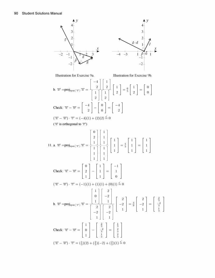
90 Student Solutions Manual
x x
y y
3 121 1
3 3
2 2
1 1
4 4
u
u=
n
n
p
p=0
v
v
−1 −3−2 −4
−1 −1
−2 −2
Illustration for Exercise 9a. Illustration for Exercise 9b.
b. −→w =projspan{−→v }−→u =
⎡⎢⎣
−4
2
⎤⎥⎦ ·
⎡⎢⎣
1
2
⎤⎥⎦
⎡⎢⎣
1
2
⎤⎥⎦ ·
⎡⎢⎣
1
2
⎤⎥⎦
[1
2
]= 0
5
[1
2
]=
[0
0
]
Check: −→u −−→w =
[−4
2
]−[
0
0
]=
[−4
2
]
(−→u −−→w ) · −→v = (−4)(1) + (2)(2)�= 0
(−→u is orthogonal to −→v )
11. a. −→w =projspan{−→v }−→u =
⎡⎢⎢⎢⎢⎣
0
2
1
⎤⎥⎥⎥⎥⎦·
⎡⎢⎢⎢⎢⎣
1
1
1
⎤⎥⎥⎥⎥⎦
⎡⎢⎢⎢⎢⎣
1
1
1
⎤⎥⎥⎥⎥⎦·
⎡⎢⎢⎢⎢⎣
1
1
1
⎤⎥⎥⎥⎥⎦
⎡⎢⎣ 1
1
1
⎤⎥⎦ = 33
⎡⎢⎣ 1
1
1
⎤⎥⎦ =
⎡⎢⎣ 1
1
1
⎤⎥⎦
Check: −→u −−→w =
⎡⎢⎣ 0
2
1
⎤⎥⎦−
⎡⎢⎣ 1
1
1
⎤⎥⎦ =
⎡⎢⎣ −1
1
0
⎤⎥⎦(−→u −−→w ) · −→v = (−1)(1) + (1)(1) + (0)(1)
�= 0
b. −→w =projspan{−→v }−→u =
⎡⎢⎢⎢⎢⎣
1
0
1
⎤⎥⎥⎥⎥⎦·
⎡⎢⎢⎢⎢⎣
2
−2
1
⎤⎥⎥⎥⎥⎦
⎡⎢⎢⎢⎢⎣
2
−2
1
⎤⎥⎥⎥⎥⎦·
⎡⎢⎢⎢⎢⎣
2
−2
1
⎤⎥⎥⎥⎥⎦
⎡⎢⎣ 2
−2
1
⎤⎥⎦ = 39
⎡⎢⎣ 2
−2
1
⎤⎥⎦ =
⎡⎢⎣23−2313
⎤⎥⎦
Check: −→u −−→w =
⎡⎢⎣ 1
0
1
⎤⎥⎦−
⎡⎢⎣23−2313
⎤⎥⎦ =
⎡⎢⎣132323
⎤⎥⎦(−→u −−→w ) · −→v = ( 13 )(2) + ( 23 )(−2) + ( 23 )(1)
�= 0
Student Solutions Manual 91
13. a. −→w =projspan{−→v }−→u =
⎡⎢⎢⎢⎢⎢⎢⎢⎢⎣
0
1
2
3
⎤⎥⎥⎥⎥⎥⎥⎥⎥⎦·
⎡⎢⎢⎢⎢⎢⎢⎢⎢⎣
1
1
−1
−1
⎤⎥⎥⎥⎥⎥⎥⎥⎥⎦
⎡⎢⎢⎢⎢⎢⎢⎢⎢⎣
1
1
−1
−1
⎤⎥⎥⎥⎥⎥⎥⎥⎥⎦·
⎡⎢⎢⎢⎢⎢⎢⎢⎢⎣
1
1
−1
−1
⎤⎥⎥⎥⎥⎥⎥⎥⎥⎦
⎡⎢⎢⎢⎢⎣1
1
−1
−1
⎤⎥⎥⎥⎥⎦ = −44
⎡⎢⎢⎢⎢⎣1
1
−1
−1
⎤⎥⎥⎥⎥⎦ =
⎡⎢⎢⎢⎢⎣−1
−1
1
1
⎤⎥⎥⎥⎥⎦
Check: −→u −−→w =
⎡⎢⎢⎢⎢⎣0
1
2
3
⎤⎥⎥⎥⎥⎦−
⎡⎢⎢⎢⎢⎣−1
−1
1
1
⎤⎥⎥⎥⎥⎦ =
⎡⎢⎢⎢⎢⎣1
2
1
2
⎤⎥⎥⎥⎥⎦(−→u −−→w ) · −→v = (1)(1) + (2)(1) + (1)(−1) + (2)(−1)
�= 0
b. −→w =projspan{−→v }−→u =
⎡⎢⎢⎢⎢⎢⎢⎢⎢⎢⎢⎢⎣
3
0
−1
1
2
⎤⎥⎥⎥⎥⎥⎥⎥⎥⎥⎥⎥⎦
·
⎡⎢⎢⎢⎢⎢⎢⎢⎢⎢⎢⎢⎣
2
1
−1
−1
−1
⎤⎥⎥⎥⎥⎥⎥⎥⎥⎥⎥⎥⎦
⎡⎢⎢⎢⎢⎢⎢⎢⎢⎢⎢⎢⎣
2
1
−1
−1
−1
⎤⎥⎥⎥⎥⎥⎥⎥⎥⎥⎥⎥⎦
·
⎡⎢⎢⎢⎢⎢⎢⎢⎢⎢⎢⎢⎣
2
1
−1
−1
−1
⎤⎥⎥⎥⎥⎥⎥⎥⎥⎥⎥⎥⎦
⎡⎢⎢⎢⎢⎢⎢⎣2
1
−1
−1
−1
⎤⎥⎥⎥⎥⎥⎥⎦ = 48
⎡⎢⎢⎢⎢⎢⎢⎣2
1
−1
−1
−1
⎤⎥⎥⎥⎥⎥⎥⎦ =
⎡⎢⎢⎢⎢⎢⎢⎣112
−12
−12
−12
⎤⎥⎥⎥⎥⎥⎥⎦
Check: −→u −−→w =
⎡⎢⎢⎢⎢⎢⎢⎣3
0
−1
1
2
⎤⎥⎥⎥⎥⎥⎥⎦−
⎡⎢⎢⎢⎢⎢⎢⎣112
−12
−12
−12
⎤⎥⎥⎥⎥⎥⎥⎦ =
⎡⎢⎢⎢⎢⎢⎢⎣2
−12
−123252
⎤⎥⎥⎥⎥⎥⎥⎦(−→u −−→w ) · −→v �
= (2)(2) + (−12 )(1) + (− 1
2 )(−1) + ( 32 )(−1) + ( 52 )(−1)�= 0.
15. Let −→w1 =
⎡⎢⎣1323
−23
⎤⎥⎦ and −→w2 =
⎡⎢⎣23
−23
−13
⎤⎥⎦We have
−→w1 · −→w2 =
⎡⎢⎣1323
− 23
⎤⎥⎦ ·
⎡⎢⎣23
−23
−13
⎤⎥⎦ = ( 13 )(23 ) + ( 23 )(−2
3 ) + (−23 )(−1
3 ) = 0,
‖−→w1‖ =√
19 + 4
9 + 49 = 1, and
‖−→w2‖ =√
49 + 4
9 + 19 = 1 therefore S is an orthonormal set.
Using formula (82),
92 Student Solutions Manual
projspanS−→u = (−→u · −→w1)−→w1 + (−→u · −→w2)−→w2 =
=
⎛⎜⎝⎡⎢⎣ 3
2
1
⎤⎥⎦ ·
⎡⎢⎣1323
−23
⎤⎥⎦⎞⎟⎠⎡⎢⎣
1323
−23
⎤⎥⎦+
⎛⎜⎝⎡⎢⎣ 3
2
1
⎤⎥⎦ ·
⎡⎢⎣23
−23
−13
⎤⎥⎦⎞⎟⎠⎡⎢⎣
23
−23
−13
⎤⎥⎦
=5
3
⎡⎢⎣1323
−23
⎤⎥⎦+1
3
⎡⎢⎣23
−23
−13
⎤⎥⎦ =
⎡⎢⎣7989
−119
⎤⎥⎦
17. Let −→w1 =
⎡⎢⎢⎢⎢⎣12121212
⎤⎥⎥⎥⎥⎦ and −→w2 =
⎡⎢⎢⎢⎢⎣12
− 12
− 1212
⎤⎥⎥⎥⎥⎦We have
−→w1 · −→w2 =
⎡⎢⎢⎢⎢⎣12121212
⎤⎥⎥⎥⎥⎦ ·
⎡⎢⎢⎢⎢⎣12
−12
−1212
⎤⎥⎥⎥⎥⎦ = ( 12)( 1
2) + ( 1
2)(−1
2) + ( 1
2)(−1
2) + ( 1
2)( 1
2) = 0,
‖−→w1‖ =√
14 + 1
4 + 14 + 1
4 = 1, and
‖−→w2‖ =√
14 + 1
4 + 14 + 1
4 = 1 therefore S is an orthonormal set.
Using formula (82),
projspanS−→u = (−→u · −→w1)−→w1 + (−→u · −→w2)−→w2 =
=
⎛⎜⎜⎜⎜⎝⎡⎢⎢⎢⎢⎣
1
−2
1
1
⎤⎥⎥⎥⎥⎦ ·
⎡⎢⎢⎢⎢⎣12121212
⎤⎥⎥⎥⎥⎦⎞⎟⎟⎟⎟⎠⎡⎢⎢⎢⎢⎣
12121212
⎤⎥⎥⎥⎥⎦+
⎛⎜⎜⎜⎜⎝⎡⎢⎢⎢⎢⎣
1
−2
1
1
⎤⎥⎥⎥⎥⎦ ·
⎡⎢⎢⎢⎢⎣12
−12
−1212
⎤⎥⎥⎥⎥⎦⎞⎟⎟⎟⎟⎠⎡⎢⎢⎢⎢⎣
12
−12
−1212
⎤⎥⎥⎥⎥⎦
=1
2
⎡⎢⎢⎢⎢⎣12121212
⎤⎥⎥⎥⎥⎦+3
2
⎡⎢⎢⎢⎢⎣12
− 12
− 1212
⎤⎥⎥⎥⎥⎦ =
⎡⎢⎢⎢⎢⎣1
− 12
− 12
1
⎤⎥⎥⎥⎥⎦
19. Let −→v1 =
⎡⎢⎣ 1
2
−1
⎤⎥⎦ and −→v2 =
⎡⎢⎣ −1
1
1
⎤⎥⎦We have
−→v1 · −→v2 =
⎡⎢⎣ 1
2
−1
⎤⎥⎦ ·
⎡⎢⎣ −1
1
1
⎤⎥⎦ = (1)(−1) + (2)(1) + (−1)(1) = 0,
therefore S is an orthogonal set.
Using formula (81),
Student Solutions Manual 93
projspanS−→u =
−→u · −→v1−→v1 · −→v1−→v1 +
−→u · −→v2−→v2 · −→v2−→v2 =
=
⎡⎢⎣ 5
2
−2
⎤⎥⎦ ·
⎡⎢⎣ 1
2
−1
⎤⎥⎦⎡⎢⎣ 1
2
−1
⎤⎥⎦ ·
⎡⎢⎣ 1
2
−1
⎤⎥⎦
⎡⎢⎣ 1
2
−1
⎤⎥⎦+
⎡⎢⎣ 5
2
−2
⎤⎥⎦ ·
⎡⎢⎣ −1
1
1
⎤⎥⎦⎡⎢⎣ −1
1
1
⎤⎥⎦ ·
⎡⎢⎣ −1
1
1
⎤⎥⎦
⎡⎢⎣ −1
1
1
⎤⎥⎦
=11
6
⎡⎢⎣ 1
2
−1
⎤⎥⎦− 5
3
⎡⎢⎣ −1
1
1
⎤⎥⎦ =
⎡⎢⎣72
2
−72
⎤⎥⎦
21. Let −→v1 =
⎡⎢⎢⎢⎢⎣1
0
1
1
⎤⎥⎥⎥⎥⎦ , −→v2 =
⎡⎢⎢⎢⎢⎣−1
−1
1
0
⎤⎥⎥⎥⎥⎦ , and −→v3 =
⎡⎢⎢⎢⎢⎣0
−1
−1
1
⎤⎥⎥⎥⎥⎦We have
−→v1 · −→v2 =
⎡⎢⎢⎢⎢⎣1
0
1
1
⎤⎥⎥⎥⎥⎦ ·
⎡⎢⎢⎢⎢⎣−1
−1
1
0
⎤⎥⎥⎥⎥⎦ = (1)(−1) + (0)(−1) + (1)(1) + (1)(0) = 0,
−→v1 · −→v3 =
⎡⎢⎢⎢⎢⎣1
0
1
1
⎤⎥⎥⎥⎥⎦ ·
⎡⎢⎢⎢⎢⎣0
−1
−1
1
⎤⎥⎥⎥⎥⎦ = (1)(0) + (0)(−1) + (1)(−1) + (1)(1) = 0, and
−→v2 · −→v3 =
⎡⎢⎢⎢⎢⎣−1
−1
1
0
⎤⎥⎥⎥⎥⎦ ·
⎡⎢⎢⎢⎢⎣0
−1
−1
1
⎤⎥⎥⎥⎥⎦ = (−1)(0) + (−1)(−1) + (1)(−1) + (0)(1) = 0,
therefore S is an orthogonal set.
Using formula (81),
94 Student Solutions Manual
projspanS−→u =
−→u · −→v1−→v1 · −→v1−→v1 +
−→u · −→v2−→v2 · −→v2−→v2 +
−→u · −→v3−→v3 · −→v3−→v3
=
⎡⎢⎢⎢⎢⎣3
0
1
2
⎤⎥⎥⎥⎥⎦ ·
⎡⎢⎢⎢⎢⎣1
0
1
1
⎤⎥⎥⎥⎥⎦⎡⎢⎢⎢⎢⎣
1
0
1
1
⎤⎥⎥⎥⎥⎦ ·
⎡⎢⎢⎢⎢⎣1
0
1
1
⎤⎥⎥⎥⎥⎦
⎡⎢⎢⎢⎢⎣1
0
1
1
⎤⎥⎥⎥⎥⎦+
⎡⎢⎢⎢⎢⎣3
0
1
2
⎤⎥⎥⎥⎥⎦ ·
⎡⎢⎢⎢⎢⎣−1
−1
1
0
⎤⎥⎥⎥⎥⎦⎡⎢⎢⎢⎢⎣
−1
−1
1
0
⎤⎥⎥⎥⎥⎦ ·
⎡⎢⎢⎢⎢⎣−1
−1
1
0
⎤⎥⎥⎥⎥⎦
⎡⎢⎢⎢⎢⎣−1
−1
1
0
⎤⎥⎥⎥⎥⎦+
⎡⎢⎢⎢⎢⎣3
0
1
2
⎤⎥⎥⎥⎥⎦ ·
⎡⎢⎢⎢⎢⎣0
−1
−1
1
⎤⎥⎥⎥⎥⎦⎡⎢⎢⎢⎢⎣
0
−1
−1
1
⎤⎥⎥⎥⎥⎦ ·
⎡⎢⎢⎢⎢⎣0
−1
−1
1
⎤⎥⎥⎥⎥⎦
⎡⎢⎢⎢⎢⎣0
−1
−1
1
⎤⎥⎥⎥⎥⎦
=5
3
⎡⎢⎢⎢⎢⎣1
0
1
1
⎤⎥⎥⎥⎥⎦− 1
3
⎡⎢⎢⎢⎢⎣−1
−1
1
0
⎤⎥⎥⎥⎥⎦+1
3
⎡⎢⎢⎢⎢⎣0
−1
−1
1
⎤⎥⎥⎥⎥⎦ =
⎡⎢⎢⎢⎢⎣8313
173
⎤⎥⎥⎥⎥⎦23. Taking −→v1 = −→v in formula (86)
B =1
−→v · −→v−→v −→v T =
1
4 + 16
[−2
4
] [−2 4
]=
1
20
[4 −8
−8 16
]=
[15
−25
−25
45
]
B−→u =
[15 −2
5
−25
45
][3
−1
]=
[1
−2
]25. Taking −→v1 = −→v in formula (86)
B =1
−→v · −→v−→v −→v T =
1
1 + 1 + 1
⎡⎢⎣ 1
1
1
⎤⎥⎦[ 1 1 1]=
1
3
⎡⎢⎣ 1 1 1
1 1 1
1 1 1
⎤⎥⎦ =
⎡⎢⎣13
13
13
13
13
13
13
13
13
⎤⎥⎦
B−→u =
⎡⎢⎣13
13
13
13
13
13
13
13
13
⎤⎥⎦⎡⎢⎣ 0
2
1
⎤⎥⎦ =
⎡⎢⎣ 1
1
1
⎤⎥⎦27. Taking −→v1 = −→v in formula (86)
B =1
−→v · −→v−→v −→v T =
1
1 + 1 + 1 + 1
⎡⎢⎢⎢⎢⎣1
1
−1
−1
⎤⎥⎥⎥⎥⎦[1 1 −1 −1
]
=1
4
⎡⎢⎢⎢⎢⎣1 1 −1 −1
1 1 −1 −1
−1 −1 1 1
−1 −1 1 1
⎤⎥⎥⎥⎥⎦ =
⎡⎢⎢⎢⎢⎣14
14 −1
4 −14
14
14
−14
−14
−14 − 1
414
14
−14 − 1
414
14
⎤⎥⎥⎥⎥⎦
Student Solutions Manual 95
B−→u =
⎡⎢⎢⎢⎢⎣14
14 −1
4 − 14
14
14 −1
4 − 14
− 14
−14
14
14
− 14 −1
414
14
⎤⎥⎥⎥⎥⎦⎡⎢⎢⎢⎢⎣
0
1
2
3
⎤⎥⎥⎥⎥⎦ =
⎡⎢⎢⎢⎢⎣−1
−1
1
1
⎤⎥⎥⎥⎥⎦29. Using formula (87),
B = AAT =
⎡⎢⎣13
23
23 − 2
3
−23 − 1
3
⎤⎥⎦[ 13
23 −2
323 − 2
3 −13
]=
⎡⎢⎣59
−29
−49
− 29
89 −2
9
− 49 −2
959
⎤⎥⎦
B−→u =
⎡⎢⎣59 −2
9 −49
− 29
89
−29
− 49 −2
959
⎤⎥⎦⎡⎢⎣ 3
2
1
⎤⎥⎦ =
⎡⎢⎣7989
−119
⎤⎥⎦31. Using formula (86),
B =1
−→v1 · −→v1−→v1−→v1T +
1−→v2 · −→v2
−→v2−→v2T +1
−→v3 · −→v3−→v3−→v3T
=1
3
⎡⎢⎢⎢⎢⎣1
0
1
1
⎤⎥⎥⎥⎥⎦[1 0 1 1
]+
1
3
⎡⎢⎢⎢⎢⎣−1
−1
1
0
⎤⎥⎥⎥⎥⎦[−1 −1 1 0
]+
1
3
⎡⎢⎢⎢⎢⎣0
−1
−1
1
⎤⎥⎥⎥⎥⎦[0 −1 −1 1
]
=1
3
⎡⎢⎢⎢⎢⎣1 0 1 1
0 0 0 0
1 0 1 1
1 0 1 1
⎤⎥⎥⎥⎥⎦+1
3
⎡⎢⎢⎢⎢⎣1 1 −1 0
1 1 −1 0
−1 −1 1 0
0 0 0 0
⎤⎥⎥⎥⎥⎦+1
3
⎡⎢⎢⎢⎢⎣0 0 0 0
0 1 1 −1
0 1 1 −1
0 −1 −1 1
⎤⎥⎥⎥⎥⎦
=
⎡⎢⎢⎢⎢⎣23
13 0 1
313
23 0 −1
3
0 0 1 013
−13
0 23
⎤⎥⎥⎥⎥⎦
B−→u =
⎡⎢⎢⎢⎢⎣23
13 0 1
313
23 0 −1
3
0 0 1 013 − 1
3 0 23
⎤⎥⎥⎥⎥⎦⎡⎢⎢⎢⎢⎣
3
0
1
2
⎤⎥⎥⎥⎥⎦ =
⎡⎢⎢⎢⎢⎣8313
173
⎤⎥⎥⎥⎥⎦
96 Student Solutions Manual
Section
6.3 1. a. −→u1 =
⎡⎢⎣ −2
1
2
⎤⎥⎦ ,−→u2 =
⎡⎢⎣ −3
2
5
⎤⎥⎦Orthogonal basis:
−→v1 = −→u1 =
⎡⎢⎣ −2
1
2
⎤⎥⎦
−→v2 = −→u2 − −→u2·−→v1−→v1 ·−→v1
−→v1 =
⎡⎢⎣ −3
2
5
⎤⎥⎦− 189
⎡⎢⎣ −2
1
2
⎤⎥⎦ =
⎡⎢⎣ 1
0
1
⎤⎥⎦ .Orthonormal basis:
−→w1 = 1‖−→v1‖
−→v1 = 1√9
⎡⎢⎣ −2
1
2
⎤⎥⎦ =
⎡⎢⎣ −23
1323
⎤⎥⎦
−→w2 = 1‖−→v2‖
−→v2 = 1√2
⎡⎢⎣ 1
0
1
⎤⎥⎦
b. −→u1 =
⎡⎢⎣ 2
1
−1
⎤⎥⎦ ,−→u2 =
⎡⎢⎣ 4
3
2
⎤⎥⎦Orthogonal basis:
−→v1 = −→u1 =
⎡⎢⎣ 2
1
−1
⎤⎥⎦−→v2 = −→u2 − −→u2·−→v1−→v1 ·−→v1
−→v1 =
⎡⎢⎣ 4
3
2
⎤⎥⎦− 96
⎡⎢⎣ 2
1
−1
⎤⎥⎦
=
⎡⎢⎣ 4
3
2
⎤⎥⎦+
⎡⎢⎣ −3−3232
⎤⎥⎦ =
⎡⎢⎣ 13272
⎤⎥⎦
We can replace −→v2 with the vector twice as long to avoid fractions: −→v2 =
⎡⎢⎣ 2
3
7
⎤⎥⎦Orthonormal basis:
−→w1 = 1‖−→v1‖
−→v1 = 1√6
⎡⎢⎣ 2
1
−1
⎤⎥⎦
Student Solutions Manual 97
−→w2 = 1‖−→v2‖
−→v2 = 1√62
⎡⎢⎣ 2
3
7
⎤⎥⎦
c. −→u1 =
⎡⎢⎢⎢⎢⎣1
1
1
1
⎤⎥⎥⎥⎥⎦ ,−→u2 =
⎡⎢⎢⎢⎢⎣6
4
0
2
⎤⎥⎥⎥⎥⎦Orthogonal basis:
−→v1 = −→u1 =
⎡⎢⎢⎢⎢⎣1
1
1
1
⎤⎥⎥⎥⎥⎦
−→v2 = −→u2 − −→u2·−→v1−→v1 ·−→v1
−→v1 =
⎡⎢⎢⎢⎢⎣6
4
0
2
⎤⎥⎥⎥⎥⎦− 124
⎡⎢⎢⎢⎢⎣1
1
1
1
⎤⎥⎥⎥⎥⎦ =
⎡⎢⎢⎢⎢⎣3
1
−3
−1
⎤⎥⎥⎥⎥⎦ .Orthonormal basis:
−→w1 = 1‖−→v1‖
−→v1 = 12
⎡⎢⎢⎢⎢⎣1
1
1
1
⎤⎥⎥⎥⎥⎦
−→w2 = 1‖−→v2‖
−→v2 = 1√20
⎡⎢⎢⎢⎢⎣3
1
−3
−1
⎤⎥⎥⎥⎥⎦
3. a. −→u1 =
⎡⎢⎢⎢⎢⎣1
2
0
2
⎤⎥⎥⎥⎥⎦ ,−→u2 =
⎡⎢⎢⎢⎢⎣−1
−3
2
−1
⎤⎥⎥⎥⎥⎦ ,−→u3 =
⎡⎢⎢⎢⎢⎣−2
−1
3
2
⎤⎥⎥⎥⎥⎦Orthogonal basis:
−→v1 = −→u1 =
⎡⎢⎢⎢⎢⎣1
2
0
2
⎤⎥⎥⎥⎥⎦
−→v2 = −→u2 − −→u2·−→v1−→v1 ·−→v1
−→v1 =
⎡⎢⎢⎢⎢⎣−1
−3
2
−1
⎤⎥⎥⎥⎥⎦− −99
⎡⎢⎢⎢⎢⎣1
2
0
2
⎤⎥⎥⎥⎥⎦ =
⎡⎢⎢⎢⎢⎣0
−1
2
1
⎤⎥⎥⎥⎥⎦−→v3 = −→u3 − −→u3·−→v1−→v1 ·−→v1
−→v1 − −→u3·−→v2−→v2 ·−→v2−→v2
98 Student Solutions Manual
=
⎡⎢⎢⎢⎢⎣−2
−1
3
2
⎤⎥⎥⎥⎥⎦− 09
⎡⎢⎢⎢⎢⎣1
2
0
2
⎤⎥⎥⎥⎥⎦− 96
⎡⎢⎢⎢⎢⎣0
−1
2
1
⎤⎥⎥⎥⎥⎦ =
⎡⎢⎢⎢⎢⎣−212
012
⎤⎥⎥⎥⎥⎦
We can replace −→v3 with the vector twice as long to avoid fractions: −→v3 =
⎡⎢⎢⎢⎢⎣−4
1
0
1
⎤⎥⎥⎥⎥⎦Orthonormal basis:
−→w1 = 1‖−→v1‖
−→v1 = 13
⎡⎢⎢⎢⎢⎣1
2
0
2
⎤⎥⎥⎥⎥⎦
−→w2 = 1‖−→v2‖
−→v2 = 1√6
⎡⎢⎢⎢⎢⎣0
−1
2
1
⎤⎥⎥⎥⎥⎦
−→w3 = 1‖−→v3‖
−→v3 = 1√18
⎡⎢⎢⎢⎢⎣−4
1
0
1
⎤⎥⎥⎥⎥⎦
b. −→u1 =
⎡⎢⎢⎢⎢⎢⎢⎣1
0
0
0
−1
⎤⎥⎥⎥⎥⎥⎥⎦ ,−→u2 =
⎡⎢⎢⎢⎢⎢⎢⎣0
2
0
0
4
⎤⎥⎥⎥⎥⎥⎥⎦ ,−→u3 =
⎡⎢⎢⎢⎢⎢⎢⎣2
0
−1
1
4
⎤⎥⎥⎥⎥⎥⎥⎦Orthogonal basis:
−→v1 = −→u1 =
⎡⎢⎢⎢⎢⎢⎢⎣1
0
0
0
−1
⎤⎥⎥⎥⎥⎥⎥⎦
−→v2 = −→u2 − −→u2·−→v1−→v1 ·−→v1
−→v1 =
⎡⎢⎢⎢⎢⎢⎢⎣0
2
0
0
4
⎤⎥⎥⎥⎥⎥⎥⎦− −42
⎡⎢⎢⎢⎢⎢⎢⎣1
0
0
0
−1
⎤⎥⎥⎥⎥⎥⎥⎦ =
⎡⎢⎢⎢⎢⎢⎢⎣2
2
0
0
2
⎤⎥⎥⎥⎥⎥⎥⎦−→v3 = −→u3 − −→u3·−→v1−→v1 ·−→v1
−→v1 − −→u3·−→v2−→v2 ·−→v2−→v2
Student Solutions Manual 99
=
⎡⎢⎢⎢⎢⎢⎢⎣2
0
−1
1
4
⎤⎥⎥⎥⎥⎥⎥⎦− −22
⎡⎢⎢⎢⎢⎢⎢⎣1
0
0
0
−1
⎤⎥⎥⎥⎥⎥⎥⎦− 1212
⎡⎢⎢⎢⎢⎢⎢⎣2
2
0
0
2
⎤⎥⎥⎥⎥⎥⎥⎦ =
⎡⎢⎢⎢⎢⎢⎢⎣1
−2
−1
1
1
⎤⎥⎥⎥⎥⎥⎥⎦Orthonormal basis:
−→w1 = 1‖−→v1‖
−→v1 = 1√2
⎡⎢⎢⎢⎢⎢⎢⎣1
0
0
0
−1
⎤⎥⎥⎥⎥⎥⎥⎦
−→w2 = 1‖−→v2‖
−→v2 = 1√12
⎡⎢⎢⎢⎢⎢⎢⎣2
2
0
0
2
⎤⎥⎥⎥⎥⎥⎥⎦ =
⎡⎢⎢⎢⎢⎢⎢⎢⎣
1√31√3
0
01√3
⎤⎥⎥⎥⎥⎥⎥⎥⎦
−→w3 = 1‖−→v3‖
−→v3 = 1√8
⎡⎢⎢⎢⎢⎢⎢⎣1
−2
−1
1
1
⎤⎥⎥⎥⎥⎥⎥⎦
5. The null space of the plane equation consists of vectors
⎡⎢⎣ x
y
z
⎤⎥⎦ =
⎡⎢⎣ y + z
y
z
⎤⎥⎦ = y
⎡⎢⎣ 1
1
0
⎤⎥⎦ + z
⎡⎢⎣ 1
0
1
⎤⎥⎦ ,so that the vectors −→u1 =
⎡⎢⎣ 1
1
0
⎤⎥⎦ , −→u2 =
⎡⎢⎣ 1
0
1
⎤⎥⎦ form a basis for V. a. To use formula (81), we need an
orthogonal basis for V, which we shall find using the Gram-Schmidt process.
−→v1 = −→u1 =
⎡⎢⎣ 1
1
0
⎤⎥⎦−→v2 = −→u2 − −→u2·−→v1−→v1 ·−→v1
−→v1 =
⎡⎢⎣ 1
0
1
⎤⎥⎦− 12
⎡⎢⎣ 1
1
0
⎤⎥⎦ =
⎡⎢⎣12−12
1
⎤⎥⎦ .
We can replace this vector with twice the same vector,
⎡⎢⎣ 1
−1
2
⎤⎥⎦ , to avoid fractions in the remaining
computations.
The matrix of the transformation is can be obtained as
1−→v1 ·−→v1−→v1−→v1 T + 1−→v2 ·−→v2
−→v2−→v2T
100 Student Solutions Manual
= 12
⎡⎢⎣ 1
1
0
⎤⎥⎦[ 1 1 0]+ 1
6
⎡⎢⎣ 1
−1
2
⎤⎥⎦[ 1 −1 2]
= 12
⎡⎢⎣ 1 1 0
1 1 0
0 0 0
⎤⎥⎦+ 16
⎡⎢⎣ 1 −1 2
−1 1 −2
2 −2 4
⎤⎥⎦
=
⎡⎢⎣23
13
13
13
23
− 13
13 −1
323
⎤⎥⎦Another way to perform the last step is to use (81) directly:
F (
⎡⎢⎣ x
y
z
⎤⎥⎦) = projspan{−→v1 ,−→v2}
⎡⎢⎣ x
y
z
⎤⎥⎦
=
⎡⎢⎣ x
y
z
⎤⎥⎦ · −→v1
−→v1 · −→v1−→v1 +
⎡⎢⎣ x
y
z
⎤⎥⎦ · −→v2
−→v2 · −→v2−→v2
=x+ y
2
⎡⎢⎣ 1
1
0
⎤⎥⎦+x− y + 2z
6
⎡⎢⎣ 1
−1
2
⎤⎥⎦
=
⎡⎢⎣23x+ 1
3y +13z
13x+ 2
3y − 13z
13x− 1
3y +23z
⎤⎥⎦
=
⎡⎢⎣23
13
13
13
23
−13
13
−13
23
⎤⎥⎦⎡⎢⎣ x
y
z
⎤⎥⎦ .(or, apply the projection to each of the standard basis vectors.)
b.
Student Solutions Manual 101
Our plane is the column space of A =
⎡⎢⎣ 1 1
1 0
0 1
⎤⎥⎦ . Using (96), we obtain the matrix of projection:
A(ATA)−1AT =
⎡⎢⎣ 1 1
1 0
0 1
⎤⎥⎦⎛⎜⎝[ 1 1 0
1 0 1
]⎡⎢⎣ 1 1
1 0
0 1
⎤⎥⎦⎞⎟⎠
−1 [1 1 0
1 0 1
]
=
⎡⎢⎣ 1 1
1 0
0 1
⎤⎥⎦([ 2 1
1 2
])−1 [1 1 0
1 0 1
]
=
⎡⎢⎣ 1 1
1 0
0 1
⎤⎥⎦[ 23
−13
−13
23
][1 1 0
1 0 1
]
=
⎡⎢⎣23
13
13
13
23 −1
313
− 13
23
⎤⎥⎦
7. The null space of the plane equation consists of vectors
⎡⎢⎣ x
y
z
⎤⎥⎦ =
⎡⎢⎣ −z
y
z
⎤⎥⎦ = y
⎡⎢⎣ 0
1
0
⎤⎥⎦+z
⎡⎢⎣ −1
0
1
⎤⎥⎦ , sothat the vectors−→u1 =
⎡⎢⎣ 0
1
0
⎤⎥⎦ ,−→u2 =
⎡⎢⎣ −1
0
1
⎤⎥⎦ form a basis forV. a. These vectors are already orthogonal,
so that we can proceed directly to use formula (81) without using the Gram-Schmidt process, taking
−→v1 = −→u1 and −→v2 = −→u2 .The matrix of the transformation is can be obtained as
1−→v1 ·−→v1−→v1−→v1 T + 1−→v2 ·−→v2
−→v2−→v2T
= 11
⎡⎢⎣ 0
1
0
⎤⎥⎦[ 0 1 0]+ 1
2
⎡⎢⎣ −1
0
1
⎤⎥⎦[ −1 0 1]
=
⎡⎢⎣ 0 0 0
0 1 0
0 0 0
⎤⎥⎦+ 12
⎡⎢⎣ 1 0 −1
0 0 0
−1 0 1
⎤⎥⎦ =
⎡⎢⎣12 0 −1
2
0 1 0
−12
0 12
⎤⎥⎦
102 Student Solutions Manual
Another way: according to (81) the transformation F can be expressed as
F (
⎡⎢⎣ x
y
z
⎤⎥⎦) = projspan{−→v1 ,−→v2}
⎡⎢⎣ x
y
z
⎤⎥⎦
=
⎡⎢⎣ x
y
z
⎤⎥⎦ · −→v1
−→v1 · −→v1−→v1 +
⎡⎢⎣ x
y
z
⎤⎥⎦ · −→v2
−→v2 · −→v2−→v2
=y
1
⎡⎢⎣ 0
1
0
⎤⎥⎦+−x+ z
2
⎡⎢⎣ −1
0
1
⎤⎥⎦
=
⎡⎢⎣12x− 1
2z
y
−12x+ 1
2z
⎤⎥⎦
=
⎡⎢⎣12 0 −1
2
0 1 0−12 0 1
2
⎤⎥⎦⎡⎢⎣ x
y
z
⎤⎥⎦ .(The same matrix A can be obtained by applying the projection to each of the standard basis vectors.)
b.
Our plane is the column space of A =
⎡⎢⎣ 0 −1
1 0
0 1
⎤⎥⎦ . Using (96), we obtain the matrix of projection:
A(ATA)−1AT =
⎡⎢⎣ 0 −1
1 0
0 1
⎤⎥⎦⎛⎜⎝[ 0 1 0
−1 0 1
]⎡⎢⎣ 0 −1
1 0
0 1
⎤⎥⎦⎞⎟⎠
−1 [0 1 0
−1 0 1
]
=
⎡⎢⎣ 0 −1
1 0
0 1
⎤⎥⎦([ 1 0
0 2
])−1 [0 1 0
−1 0 1
]
=
⎡⎢⎣ 0 −1
1 0
0 1
⎤⎥⎦[ 1 0
0 12
][0 1 0
−1 0 1
]
=
⎡⎢⎣12 0 − 1
2
0 1 0
−12 0 1
2
⎤⎥⎦
9. −→x = (ATA)−1AT−→b =
⎛⎜⎝[ 1 1 0
2 1 1
]⎡⎢⎣ 1 2
1 1
0 1
⎤⎥⎦⎞⎟⎠
−1 [1 1 0
2 1 1
]⎡⎢⎣ 1
3
1
⎤⎥⎦
=
([2 3
3 6
])−1 [1 1 0
2 1 1
]⎡⎢⎣ 1
3
1
⎤⎥⎦ =
[2 −1
−1 23
][1 1 0
2 1 1
] ⎡⎢⎣ 1
3
1
⎤⎥⎦ =
[2
0
]
Student Solutions Manual 103
11. −→x = (ATA)−1AT−→b =
⎛⎜⎜⎜⎜⎝[
1 1 −1 1
−2 −2 1 −1
]⎡⎢⎢⎢⎢⎣1 −2
1 −2
−1 1
1 −1
⎤⎥⎥⎥⎥⎦⎞⎟⎟⎟⎟⎠
−1 [1 1 −1 1
−2 −2 1 −1
]⎡⎢⎢⎢⎢⎣2
0
2
6
⎤⎥⎥⎥⎥⎦
=
([4 −6
−6 10
])−1 [1 1 −1 1
−2 −2 1 −1
]⎡⎢⎢⎢⎢⎣2
0
2
6
⎤⎥⎥⎥⎥⎦ =
[52
32
32 1
][1 1 −1 1
−2 −2 1 −1
]⎡⎢⎢⎢⎢⎣2
0
2
6
⎤⎥⎥⎥⎥⎦ =
[3
1
].
13. The normal equation
ATA−→x = AT−→b
has ATA =
⎡⎢⎣ 1 2
0 0
2 4
⎤⎥⎦[ 1 0 2
2 0 4
]=
⎡⎢⎣ 5 0 10
0 0 0
10 0 20
⎤⎥⎦
The right hand side becomes AT−→b =
⎡⎢⎣ 1 2
0 0
2 4
⎤⎥⎦[ 1
1
]=
⎡⎢⎣ 3
0
6
⎤⎥⎦
The normal equation leads to a linear system with the augmented matrix
⎡⎢⎣ 5 0 10 3
0 0 0 0
10 0 20 6
⎤⎥⎦ with the
reduced row echelon form:
⎡⎢⎣ 1 0 2 35
0 0 0 0
0 0 0 0
⎤⎥⎦ .Therefore, the solutions satisfy
x1 =3
5− 2x3
x2 = arbitrary
x3 = arbitrary
104 Student Solutions Manual
Section
7.11. A−→u1 = −1
2−→u1 , therefore the correct answer is: (f) the given vector is an eigenvector of A associated with
λ = −12 .
3. A−→u3 = 2−→u3 , therefore the correct answer is: (c) the given vector is an eigenvector of A associated with
λ = 2.
5. (a) iv; (b) i; (c) ii;
7.a. Characteristic polynomial:
det(λI2 −A) = det
[λ− 2 −4
−1 λ+ 1
]= λ2 − λ− 6 = (λ+ 2)(λ− 3)
The eigenvalues are −2 and 3.
b. Characteristic polynomial:
det(λI3 −A) = det
⎡⎢⎣ λ −2 0
−1 λ+ 1 0
0 −2 λ+ 3
⎤⎥⎦Expand along the third column
= (λ+ 3) det
[λ −2
−1 λ+ 1
]= (λ+ 3) [λ (λ +1) − 2]
= (λ+ 3) (λ2 + λ − 2) = (λ+ 3)(λ+ 2)(λ− 1)
The eigenvalues are 1, −2 and −3.
9. A =
⎡⎢⎣ −1 4 0
3 −2 0
2 0 4
⎤⎥⎦ has eigenvalues λ1 = 4, λ2 = −5, and λ3 = 2.
For λ1 = 4 the coefficient matrix of the homogeneous system is
(4)I3 −A =
⎡⎢⎣ 5 −4 0
−3 6 0
−2 0 0
⎤⎥⎦
The r.r.e.f. is
⎡⎢⎣ 1 0 0
0 1 0
0 0 0
⎤⎥⎦ so that the corresponding eigenvectors are of the form
⎡⎢⎣ x1
x2
x3
⎤⎥⎦ =
⎡⎢⎣ 0
0
x3
⎤⎥⎦ = x3
⎡⎢⎣ 0
0
1
⎤⎥⎦with x3 �= 0.
The eigenspace has basis
⎡⎢⎣ 0
0
1
⎤⎥⎦ .For λ2 = −5 the coefficient matrix of the homogeneous system is
(−5)I3 −A =
⎡⎢⎣ −4 −4 0
−3 −3 0
−2 0 −9
⎤⎥⎦
Student Solutions Manual 105
The r.r.e.f. is
⎡⎢⎣ 1 0 92
0 1 −92
0 0 0
⎤⎥⎦ so that the corresponding eigenvectors are of the form
⎡⎢⎣ x1
x2
x3
⎤⎥⎦ =
⎡⎢⎣ −92x3
92x3
x3
⎤⎥⎦ = x3
⎡⎢⎣ −92
92
1
⎤⎥⎦with x3 �= 0.
The eigenspace has basis
⎡⎢⎣ −92
92
1
⎤⎥⎦ .For λ3 = 2 the coefficient matrix of the homogeneous system is
(2)I3 −A =
⎡⎢⎣ 3 −4 0
−3 4 0
−2 0 −2
⎤⎥⎦
The r.r.e.f. is
⎡⎢⎣ 1 0 1
0 1 34
0 0 0
⎤⎥⎦ so that the corresponding eigenvectors are of the form
⎡⎢⎣ x1
x2
x3
⎤⎥⎦ =
⎡⎢⎣ −x3−34 x3
x3
⎤⎥⎦ = x3
⎡⎢⎣ −1−34
1
⎤⎥⎦with x3 �= 0.
The eigenspace has basis
⎡⎢⎣ −1−34
1
⎤⎥⎦ .11.a. Characteristic polynomial:
det(λI2 −A) = det
[λ− 4 −2
0 λ− 1
]= (λ − 4)(λ − 1)
The eigenvalues are 4 and 1 (both with algebraic multiplicity 1).
For λ1 = 4 the coefficient matrix of the homogeneous system is
(4)I2 −A =
[0 −2
0 3
]
The r.r.e.f. is
[0 1
0 0
]so that the corresponding eigenvectors are of the form[
x1
x2
]=
[x1
0
]= x1
[1
0
]with x1 �= 0.
The eigenspace has basis
[1
0
].
For λ1 = 1 the coefficient matrix of the homogeneous system is
(1)I2 −A =
[−3 −2
0 0
]
106 Student Solutions Manual
The r.r.e.f. is
[1 2
3
0 0
]so that the corresponding eigenvectors are of the form[
x1
x2
]=
[−2
3x2
x2
]= x2
[−2
3
1
]with x2 �= 0.
The eigenspace has basis
[− 2
3
1
].
b. Characteristic polynomial:
det(λI2 −A) = det
[λ− 6 −5
−1 λ− 2
]= (λ − 6)(λ − 2)− 5
= λ2 − 8λ+ 7 = (λ − 1)(λ − 7).
The eigenvalues are 1 and 7 (both with algebraic multiplicity 1).
For λ1 = 1 the coefficient matrix of the homogeneous system is
(1)I2 −A =
[−5 −5
−1 −1
]
The r.r.e.f. is
[1 1
0 0
]so that the corresponding eigenvectors are of the form[
x1
x2
]=
[−x2
x2
]= x2
[−1
1
]with x2 �= 0.
The eigenspace has basis
[−1
1
].
For λ1 = 7 the coefficient matrix of the homogeneous system is
(−2)I2 −A =
[1 −5
−1 5
]
The r.r.e.f. is
[1 −5
0 0
]so that the corresponding eigenvectors are of the form[
x1
x2
]=
[5x2
x2
]= x2
[5
1
]with x2 �= 0.
The eigenspace has basis
[5
1
].
c. Characteristic polynomial:
det(λI2 −A) = det
[λ− 1 2
−8 λ− 9
]= (λ − 1)(λ − 9) + 16
= λ2 − 10λ+ 25 = (λ− 5)2
The only eigenvalue is 5, with algebraic multiplicity 2.
For this eigenvalue, the coefficient matrix of the homogeneous system is
(5)I2 −A =
[4 2
−8 −4
]
Student Solutions Manual 107
The r.r.e.f. is
[1 1
2
0 0
]so that the corresponding eigenvectors are of the form[
x1
x2
]=
[−12 x2
x2
]= x2
[−12
1
]with x2 �= 0.
The eigenspace has basis
[−12
1
].
13.a. Characteristic polynomial:
det(λI3 −A) = det
⎡⎢⎣ λ 0 0
0 λ− 4 −2
1 0 λ +3
⎤⎥⎦ = λ(λ− 4)(λ+ 3).
The eigenvalues are 0, 4 and −3 (all with multiplicities 1).
For λ1 = 0 the coefficient matrix of the homogeneous system is
(0)I3 −A =
⎡⎢⎣ 0 0 0
0 −4 −2
1 0 3
⎤⎥⎦
The r.r.e.f. is
⎡⎢⎣ 1 0 3
0 1 12
0 0 0
⎤⎥⎦ so that the corresponding eigenvectors are of the form
⎡⎢⎣ x1
x2
x3
⎤⎥⎦ =
⎡⎢⎣ −3x3
−12 x3
x3
⎤⎥⎦ = x3
⎡⎢⎣ −3−12
1
⎤⎥⎦with x3 �= 0.
The eigenspace has basis
⎡⎢⎣ −3−12
1
⎤⎥⎦ .For λ2 = 4 the coefficient matrix of the homogeneous system is
(4)I3 −A =
⎡⎢⎣ 4 0 0
0 0 −2
1 0 7
⎤⎥⎦
The r.r.e.f. is
⎡⎢⎣ 1 0 0
0 0 1
0 0 0
⎤⎥⎦ so that the corresponding eigenvectors are of the form
⎡⎢⎣ x1
x2
x3
⎤⎥⎦ =
⎡⎢⎣ 0
x2
0
⎤⎥⎦ = x2
⎡⎢⎣ 0
1
0
⎤⎥⎦with x2 �= 0.
The eigenspace has basis
⎡⎢⎣ 0
1
0
⎤⎥⎦ .
108 Student Solutions Manual
For λ3 = −3 the coefficient matrix of the homogeneous system is
(−3)I3 −A =
⎡⎢⎣ −3 0 0
0 −7 −2
1 0 0
⎤⎥⎦
The r.r.e.f. is
⎡⎢⎣ 1 0 0
0 1 27
0 0 0
⎤⎥⎦ so that the corresponding eigenvectors are of the form
⎡⎢⎣ x1
x2
x3
⎤⎥⎦ =
⎡⎢⎣ 0−27 x3
x3
⎤⎥⎦ = x3
⎡⎢⎣ 0−27
1
⎤⎥⎦with x3 �= 0.
The eigenspace has basis
⎡⎢⎣ 0−27
1
⎤⎥⎦ .b. Characteristic polynomial:
det(λI3 −A) = det
⎡⎢⎣ λ − 2 0 0
0 λ +2 2
0 2 λ− 1
⎤⎥⎦= (λ− 2) [(λ +2) (λ − 1)− 4] = (λ− 2)
[λ2 + λ − 6
]= (λ− 2)2(λ +3)
The eigenvalues are 2 (with algebraic multiplicity 2) and −3 (with algebraic multiplicity 1).
For λ1 = 2 the coefficient matrix of the homogeneous system is
(2)I3 −A =
⎡⎢⎣ 0 0 0
0 4 2
0 2 1
⎤⎥⎦
The r.r.e.f. is
⎡⎢⎣ 0 1 12
0 0 0
0 0 0
⎤⎥⎦ so that the corresponding eigenvectors are of the form
⎡⎢⎣ x1
x2
x3
⎤⎥⎦ =
⎡⎢⎣ x1
−12 x3
x3
⎤⎥⎦ = x1
⎡⎢⎣ 1
0
0
⎤⎥⎦+ x3
⎡⎢⎣ 0−12
1
⎤⎥⎦with x1, x3 �= 0.
The eigenspace has basis
⎡⎢⎣ 1
0
0
⎤⎥⎦ ,⎡⎢⎣ 0
−12
1
⎤⎥⎦ .For λ2 = −3 the coefficient matrix of the homogeneous system is
(−3)I3 −A =
⎡⎢⎣ −5 0 0
0 −1 2
0 2 −4
⎤⎥⎦
Student Solutions Manual 109
The r.r.e.f. is
⎡⎢⎣ 1 0 0
0 1 −2
0 0 0
⎤⎥⎦ so that the corresponding eigenvectors are of the form
⎡⎢⎣ x1
x2
x3
⎤⎥⎦ =
⎡⎢⎣ 0
2x3
x3
⎤⎥⎦ = x3
⎡⎢⎣ 0
2
1
⎤⎥⎦with x3 �= 0.
The eigenspace has basis
⎡⎢⎣ 0
2
1
⎤⎥⎦ .c. Characteristic polynomial:
det(λI3 −A) = det
⎡⎢⎣ λ − 1 4 −4
−2 λ − 2 −4
0 −2 λ+ 1
⎤⎥⎦= (λ− 1)(λ− 2)(λ+ 1)− 16− 8(λ− 1) + 8(λ +1)
= λ3 − 2λ2 − λ+ 2
You may be able to notice that this polynomial can be factored:
λ3 − 2λ2 − λ+ 2 = (λ− 2)(λ2 − 1) = (λ− 2)(λ− 1)(λ+ 1)
If not, then search among the factors of the free term 2 (1,−1,2,−2) for a zero:
trying λ = 1 leads to 13 − 2(12) − 1 + 2 = 0 so that λ − 1 must be a factor in the characteristic
polynomial. Dividing
λ2 − λ − 2
−− − −− − −− − −−(λ− 1) | λ3 − 2λ2 − λ + 2
−λ3 + λ2
−− − −− − −− − −−− λ2 − λ + 2
+ λ2 − λ
−− − −− − −−− 2λ + 2
+ 2λ − 2
−− − −−0
we obtain
λ3 − 2λ2 − λ+ 2 = (λ− 1)(λ2 − λ − 2
)= (λ− 1)(λ− 2)(λ+ 1).
Either way, we arrive at the eigenvalues λ1 = 1, λ2 = 2, and λ3 = −1 (all with multiplicities 1).
For λ1 = 1 the coefficient matrix of the homogeneous system is
(1)I3 −A =
⎡⎢⎣ 0 4 −4
−2 −1 −4
0 −2 2
⎤⎥⎦
110 Student Solutions Manual
The r.r.e.f. is
⎡⎢⎣ 1 0 52
0 1 −1
0 0 0
⎤⎥⎦ so that the corresponding eigenvectors are of the form
⎡⎢⎣ x1
x2
x3
⎤⎥⎦ =
⎡⎢⎣−52 x3
x3
x3
⎤⎥⎦ = x3
⎡⎢⎣−52
1
1
⎤⎥⎦with x3 �= 0.
The eigenspace has basis
⎡⎢⎣−52
1
1
⎤⎥⎦ .For λ2 = 2 the coefficient matrix of the homogeneous system is
(2)I3 −A =
⎡⎢⎣ 1 4 −4
−2 0 −4
0 −2 3
⎤⎥⎦
The r.r.e.f. is
⎡⎢⎣ 1 0 2
0 1 −32
0 0 0
⎤⎥⎦ so that the corresponding eigenvectors are of the form
⎡⎢⎣ x1
x2
x3
⎤⎥⎦ =
⎡⎢⎣ −2x3
32x3
x3
⎤⎥⎦ = x3
⎡⎢⎣ −232
1
⎤⎥⎦with x3 �= 0.
The eigenspace has basis
⎡⎢⎣ −232
1
⎤⎥⎦ .For λ3 = −1 the coefficient matrix of the homogeneous system is
(−3)I3 −A =
⎡⎢⎣ −2 4 −4
−2 −3 −4
0 −2 0
⎤⎥⎦
The r.r.e.f. is
⎡⎢⎣ 1 0 2
0 1 0
0 0 0
⎤⎥⎦ so that the corresponding eigenvectors are of the form
⎡⎢⎣ x1
x2
x3
⎤⎥⎦ =
⎡⎢⎣ −2x3
0
x3
⎤⎥⎦ = x3
⎡⎢⎣ −2
0
1
⎤⎥⎦with x3 �= 0.
The eigenspace has basis
⎡⎢⎣ −2
0
1
⎤⎥⎦ .d. Characteristic polynomial:
Student Solutions Manual 111
det(λI3 −A) = det
⎡⎢⎣ λ −1 0
−1 λ 2
−1 1 λ
⎤⎥⎦ = λ3 + 2− 2λ − λ
= λ3 − 3λ+ 2
Search among the factors of the free term 2: 1,−1, 2,−2
trying λ = 1 leads to 13 − 3 (1) + 2 = 0 so that 1 is a root;
λ− 1 must be a factor in the characteristic polynomial. Dividing
λ2 + λ − 2
−− − −− − −− − −−(λ− 1) | λ3 − 3λ + 2
−λ3 + λ2
−− − −− − −− − −−λ2 − 3λ + 2
− λ2 + λ
−− − −− − −−− 2λ + 2
+ 2λ − 2
−− − −−0
we obtain
λ3 − 3λ+ 2 = (λ − 1)(λ2 + λ − 2
)= (λ − 1)(λ − 1)(λ +2).
Either way, we arrive at one double eigenvalue λ1 = 1, and one single eigenvalue λ2 = −2.
For λ1 = 1 the coefficient matrix of the homogeneous system is
1I3 −A =
⎡⎢⎣ 1 −1 0
−1 1 2
−1 1 1
⎤⎥⎦
The r.r.e.f. is
⎡⎢⎣ 1 −1 0
0 0 1
0 0 0
⎤⎥⎦ so that the corresponding eigenvectors are of the form
⎡⎢⎣ x1
x2
x3
⎤⎥⎦ =
⎡⎢⎣ x2
x2
0
⎤⎥⎦ = x2
⎡⎢⎣ 1
1
0
⎤⎥⎦with x2 �= 0.
The eigenspace has basis
⎡⎢⎣ 1
1
0
⎤⎥⎦ .For λ2 = −2 the coefficient matrix of the homogeneous system is
−2I3 −A =
⎡⎢⎣ −2 −1 0
−1 −2 2
−1 1 −2
⎤⎥⎦
112 Student Solutions Manual
The r.r.e.f. is
⎡⎢⎣ 1 0 23
0 1 −43
0 0 0
⎤⎥⎦ so that the corresponding eigenvectors are of the form
⎡⎢⎣ x1
x2
x3
⎤⎥⎦ =
⎡⎢⎣ −23x3
43x3
x3
⎤⎥⎦ = x3
⎡⎢⎣ −23
43
1
⎤⎥⎦with x3 �= 0.
The eigenspace has basis
⎡⎢⎣ −23
43
1
⎤⎥⎦ .15. Characteristic polynomial:
det(λI4 −A) = det
⎡⎢⎢⎢⎢⎣λ − 1 0 0 0
0 λ 0 0
−3 −3 λ+ 1 −1
2 −3 0 λ
⎤⎥⎥⎥⎥⎦Expand along the third column:
= (λ+ 1) det
⎡⎢⎣ λ− 1 0 0
0 λ 0
2 −3 λ
⎤⎥⎦expand the 3× 3 determinant along the second row
= (λ+ 1)λ det
[λ − 1 0
2 λ
]= (λ +1)λ2(λ − 1)
The eigenvalues are
• λ1 = −1 (algebraic multiplicity1),
• λ2 = 0, (algebraic multiplicity2) and
• λ3 = 1 (algebraic multiplicity 1).
For λ1 = −1 the coefficient matrix of the homogeneous system is
(−1)I4 −A =
⎡⎢⎢⎢⎢⎣−2 0 0 0
0 −1 0 0
−3 −3 0 −1
2 −3 0 −1
⎤⎥⎥⎥⎥⎦
The r.r.e.f. is
⎡⎢⎢⎢⎢⎣1 0 0 0
0 1 0 0
0 0 0 1
0 0 0 0
⎤⎥⎥⎥⎥⎦ so that the corresponding eigenvectors are of the form
⎡⎢⎢⎢⎢⎣x1
x2
x3
x4
⎤⎥⎥⎥⎥⎦ =
⎡⎢⎢⎢⎢⎣0
0
x3
0
⎤⎥⎥⎥⎥⎦ = x3
⎡⎢⎢⎢⎢⎣0
0
1
0
⎤⎥⎥⎥⎥⎦with x3 �= 0.
Student Solutions Manual 113
The eigenspace has basis
⎡⎢⎢⎢⎢⎣0
0
1
0
⎤⎥⎥⎥⎥⎦ .For λ2 = 0 the coefficient matrix of the homogeneous system is
0I4 −A =
⎡⎢⎢⎢⎢⎣−1 0 0 0
0 0 0 0
−3 −3 1 −1
2 −3 0 0
⎤⎥⎥⎥⎥⎦
The r.r.e.f. is
⎡⎢⎢⎢⎢⎣1 0 0 0
0 1 0 0
0 0 1 −1
0 0 0 0
⎤⎥⎥⎥⎥⎦ so that the corresponding eigenvectors are of the form
⎡⎢⎢⎢⎢⎣x1
x2
x3
x4
⎤⎥⎥⎥⎥⎦ =
⎡⎢⎢⎢⎢⎣0
0
x4
x4
⎤⎥⎥⎥⎥⎦ = x4
⎡⎢⎢⎢⎢⎣0
0
1
1
⎤⎥⎥⎥⎥⎦with x4 �= 0.
The eigenspace has basis
⎡⎢⎢⎢⎢⎣0
0
1
1
⎤⎥⎥⎥⎥⎦ .For λ3 = 1 the coefficient matrix of the homogeneous system is
1I4 −A =
⎡⎢⎢⎢⎢⎣0 0 0 0
0 1 0 0
−3 −3 2 −1
2 −3 0 1
⎤⎥⎥⎥⎥⎦
The r.r.e.f. is
⎡⎢⎢⎢⎢⎣1 0 0 1
2
0 1 0 0
0 0 1 14
0 0 0 0
⎤⎥⎥⎥⎥⎦ so that the corresponding eigenvectors are of the form
⎡⎢⎢⎢⎢⎣x1
x2
x3
x4
⎤⎥⎥⎥⎥⎦ =
⎡⎢⎢⎢⎢⎣−12 x4
0−14x4
x4
⎤⎥⎥⎥⎥⎦ = x4
⎡⎢⎢⎢⎢⎣−12
0−14
1
⎤⎥⎥⎥⎥⎦with x4 �= 0.
The eigenspace has basis
⎡⎢⎢⎢⎢⎣−12
0−14
1
⎤⎥⎥⎥⎥⎦ .17. FALSE
Equivalent statements imply A cannot have a zero eigenvalue
114 Student Solutions Manual
19. TRUE
A
[0
y
]= 2
[0
y
]21. FALSE
λ = −1 is an eigenvalue of A since det((−1)I −A) = 0 if and only if det(A+ I) = 0
23. TRUE
λI −A is also a scalar matrix, with all main diagonal entries λ − c
det(λI −A)=(λ − c)n
Student Solutions Manual 115
Section
7.21.a. Characteristic polynomial:
det(λI2 −A) = det
[λ− 6 6
−6 λ+ 7
]= λ2 + λ− 6 = (λ+ 3) (λ− 2)
For λ = −3, the coefficient matrix of the homogeneous system is
[−9 6
−6 4
], with r.r.e.f.
[1 −2
3
0 0
].
Eigenvectors are
[x1
x2
]= x2
[23
1
]with x2 �= 0 (e.g.,
[2
3
])
For λ = 2, the coefficient matrix of the homogeneous system is
[−4 6
−6 9
], with r.r.e.f.
[1 −3
2
0 0
].
Eigenvectors are
[x1
x2
]= x2
[32
1
]with x2 �= 0 (e.g.,
[3
2
]).
A is diagonalizable: P−1AP = D with P =
[2 3
3 2
]andD =
[−3 0
0 2
].
Verify: AP =
[6 −6
6 −7
][2 3
3 2
]=
[−6 6
−9 4
].
PD =
[2 3
3 2
][−3 0
0 2
]=
[−6 6
−9 4
]�
b. Characteristic polynomial:
det(λI2 −A) = det
[λ+ 5 2
−2 λ+ 1
]= λ2 + 6λ +9 = (λ +3)2
λ = −3 is the only eigenvalue, of algebraic multiplicity 2.
For λ = −3, the coefficient matrix of the homogeneous system is
[2 2
−2 −2
], with r.r.e.f.
[1 1
0 0
].
Eigenvectors are
[x1
x2
]= x2
[−1
1
]with x2 �= 0 (e.g.,
[−1
1
])
This eigenspace has dimension 1, therefore, it cannot yield 2 linearly independent eigenvectors required
for diagonalization.
A is not diagonalizable.
c. Characteristic polynomial:
det(λI3 −A) = det
⎡⎢⎣ λ − 3 −2 −2
1 λ −2
0 0 λ
⎤⎥⎦Expand along the third row
= λ [(λ− 3) (λ) + 2] = (λ)[λ2 − 3λ +2
]= (λ) (λ − 1) (λ− 2) .
For λ = 0, the coefficient matrix of the homogeneous system is
⎡⎢⎣ −3 −2 −2
1 0 −2
0 0 0
⎤⎥⎦, with r.r.e.f.
116 Student Solutions Manual⎡⎢⎣ 1 0 −2
0 1 4
0 0 0
⎤⎥⎦ . Eigenvectors are⎡⎢⎣ x1
x2
x3
⎤⎥⎦ = x3
⎡⎢⎣ 2
−4
1
⎤⎥⎦ with x3 �= 0 (e.g.,
⎡⎢⎣ 2
−4
1
⎤⎥⎦)
For λ = 1, the coefficient matrix of the homogeneous system is
⎡⎢⎣ −2 −2 −2
1 1 −2
0 0 1
⎤⎥⎦, with r.r.e.f.⎡⎢⎣ 1 1 0
0 0 1
0 0 0
⎤⎥⎦ . Eigenvectors are⎡⎢⎣ x1
x2
x3
⎤⎥⎦ = x2
⎡⎢⎣ −1
1
0
⎤⎥⎦ with x2 �= 0 (e.g.,
⎡⎢⎣ −1
1
0
⎤⎥⎦).
For λ = 2, the coefficient matrix of the homogeneous system is
⎡⎢⎣ −1 −2 −2
1 2 −2
0 0 2
⎤⎥⎦, with r.r.e.f.⎡⎢⎣ 1 2 0
0 0 1
0 0 0
⎤⎥⎦ . Eigenvectors are⎡⎢⎣ x1
x2
x3
⎤⎥⎦ = x2
⎡⎢⎣ −2
1
0
⎤⎥⎦ with x2 �= 0 (e.g.,
⎡⎢⎣ −2
1
0
⎤⎥⎦).
A is diagonalizable: P−1AP = D with P =
⎡⎢⎣ 2 −1 −2
−4 1 1
1 0 0
⎤⎥⎦ andD =
⎡⎢⎣ 0 0 0
0 1 0
0 0 2
⎤⎥⎦ .
Verify: AP =
⎡⎢⎣ 3 2 2
−1 0 2
0 0 0
⎤⎥⎦⎡⎢⎣ 2 −1 −2
−4 1 1
1 0 0
⎤⎥⎦ =
⎡⎢⎣ 0 −1 −4
0 1 2
0 0 0
⎤⎥⎦ .
PD =
⎡⎢⎣ 2 −1 −2
−4 1 1
1 0 0
⎤⎥⎦⎡⎢⎣ 0 0 0
0 1 0
0 0 2
⎤⎥⎦ =
⎡⎢⎣ 0 −1 −4
0 1 2
0 0 0
⎤⎥⎦�
3.a. Characteristic polynomial:
det(λI3 −A) = det
⎡⎢⎣ λ − 2 4 −3
−1 λ +2 −1
4 0 λ+ 6
⎤⎥⎦ = λ3 + 6λ2 + 12λ +8
Test factors of the free term, 8 (1,−1, 2,−1,4,−4, 8,−8).
det(1I3 −A) = 1 + 6 + 12 + 8 = 27 �= 0⇒ 1 is not an eigenvalue of A
det(−1I3 −A) = −1 + 6− 12 + 8 = 1 �= 0⇒−1 is not an eigenvalue of A
det(2I3 −A) = 8 + 6(4) + 12(2) + 8 = 64 �= 0⇒ 2 is not an eigenvalue of A
det(−2I3 −A) = −8 + 6(4) + 12(−2) + 8 = 0⇒−2 is an eigenvalue of A.
Student Solutions Manual 117
Therefore, (λ +2) is a factor of the characteristic polynomial. Use long division:
λ2 + 4λ + 4
−− − −− − −− − −−(λ +2) | λ3 + 6λ2 + 12λ + 8
−λ3 − 2λ2
−− − −− − −− − −−4λ2 + 12λ + 8
− 4λ2 − 8λ
−− − −− − −−4λ + 8
− 4λ − 8
−− − −−0
Since det(λI3 −A) = (λ+2)(λ2 + 4λ+ 4
)= (λ+2)3, it follows that λ = −2 is the only eigenvalue
with algebraic multiplicity 3
For this eigenvalue, the coefficient matrix of the homogeneous system is
⎡⎢⎣ −4 4 −3
−1 0 −1
4 0 4
⎤⎥⎦ , with r.r.e.f.
⎡⎢⎣ 1 0 1
0 1 14
0 0 0
⎤⎥⎦ . Eigenvectors are⎡⎢⎣ x1
x2
x3
⎤⎥⎦ = x3
⎡⎢⎣ −1−14
1
⎤⎥⎦ with x3 �= 0.
This eigenspace has dimension 1, therefore, it cannot yield 3 linearly independent eigenvectors required
for diagonalization.
A is not diagonalizable.
b. Characteristic polynomial:
det(λI4 −A) = det
⎡⎢⎢⎢⎢⎣λ 2 −1 1
0 λ+ 1 0 0
0 −1 λ − 2 2
0 0 0 λ +2
⎤⎥⎥⎥⎥⎦Expand along the first column:
det(λI4 −A) = λ det
⎡⎢⎣ λ +1 0 0
−1 λ− 2 2
0 0 λ+ 2
⎤⎥⎦... now, expand along the first row
det(λI4 −A) = λ (λ +1) det
[λ− 2 2
0 λ+ 2
]= λ (λ +1) (λ − 2) (λ +2) .
The matrix has four eigenvalues: 0, −1, 2, and −2 - all with algebraic multiplicity 1.
For λ = 0, the coefficient matrix of the homogeneous system is
⎡⎢⎢⎢⎢⎣0 2 −1 1
0 1 0 0
0 −1 −2 2
0 0 0 2
⎤⎥⎥⎥⎥⎦ with r.r.e.f.
118 Student Solutions Manual⎡⎢⎢⎢⎢⎣0 1 0 0
0 0 1 0
0 0 0 1
0 0 0 0
⎤⎥⎥⎥⎥⎦ . Eigenvectors are⎡⎢⎢⎢⎢⎣
x1
x2
x3
x4
⎤⎥⎥⎥⎥⎦ = x1
⎡⎢⎢⎢⎢⎣1
0
0
0
⎤⎥⎥⎥⎥⎦ with x1 �= 0 (e.g.,
⎡⎢⎢⎢⎢⎣1
0
0
0
⎤⎥⎥⎥⎥⎦)
For λ = −1, the coefficient matrix of the homogeneous system is
⎡⎢⎢⎢⎢⎣−1 2 −1 1
0 0 0 0
0 −1 −3 2
0 0 0 1
⎤⎥⎥⎥⎥⎦, with r.r.e.f.
⎡⎢⎢⎢⎢⎣1 0 7 0
0 1 3 0
0 0 0 1
0 0 0 0
⎤⎥⎥⎥⎥⎦ . Eigenvectors are⎡⎢⎢⎢⎢⎣
x1
x2
x3
x4
⎤⎥⎥⎥⎥⎦ = x3
⎡⎢⎢⎢⎢⎣−7
−3
1
0
⎤⎥⎥⎥⎥⎦ with x3 �= 0 (e.g.,
⎡⎢⎢⎢⎢⎣−7
−3
1
0
⎤⎥⎥⎥⎥⎦).
For λ = 2, the coefficient matrix of the homogeneous system is
⎡⎢⎢⎢⎢⎣2 2 −1 1
0 3 0 0
0 −1 0 2
0 0 0 4
⎤⎥⎥⎥⎥⎦ with r.r.e.f.
⎡⎢⎢⎢⎢⎣1 0 −1
2 0
0 1 0 0
0 0 0 1
0 0 0 0
⎤⎥⎥⎥⎥⎦ . Eigenvectors are⎡⎢⎢⎢⎢⎣
x1
x2
x3
x4
⎤⎥⎥⎥⎥⎦ = x3
⎡⎢⎢⎢⎢⎣12
0
1
0
⎤⎥⎥⎥⎥⎦ with x3 �= 0 (e.g.,
⎡⎢⎢⎢⎢⎣1
0
2
0
⎤⎥⎥⎥⎥⎦)
For λ = −2, the coefficient matrix of the homogeneous system is
⎡⎢⎢⎢⎢⎣−2 2 −1 1
0 −1 0 0
0 −1 −4 2
0 0 0 0
⎤⎥⎥⎥⎥⎦, with r.r.e.f.
⎡⎢⎢⎢⎢⎣1 0 0 −1
4
0 1 0 0
0 0 1 −12
0 0 0 0
⎤⎥⎥⎥⎥⎦ . Eigenvectors are⎡⎢⎢⎢⎢⎣
x1
x2
x3
x4
⎤⎥⎥⎥⎥⎦ = x4
⎡⎢⎢⎢⎢⎣14
012
1
⎤⎥⎥⎥⎥⎦ with x4 �= 0 (e.g.,
⎡⎢⎢⎢⎢⎣1
0
2
4
⎤⎥⎥⎥⎥⎦).
A is diagonalizable: P−1AP = D with P =
⎡⎢⎢⎢⎢⎣1 −7 1 1
0 −3 0 0
0 1 2 2
0 0 0 4
⎤⎥⎥⎥⎥⎦ andD =
⎡⎢⎢⎢⎢⎣0 0 0 0
0 −1 0 0
0 0 2 0
0 0 0 −2
⎤⎥⎥⎥⎥⎦ .
Verify: AP =
⎡⎢⎢⎢⎢⎣0 −2 1 −1
0 −1 0 0
0 1 2 −2
0 0 0 −2
⎤⎥⎥⎥⎥⎦⎡⎢⎢⎢⎢⎣
1 −7 1 1
0 −3 0 0
0 1 2 2
0 0 0 4
⎤⎥⎥⎥⎥⎦ =
⎡⎢⎢⎢⎢⎣0 7 2 −2
0 3 0 0
0 −1 4 −4
0 0 0 −8
⎤⎥⎥⎥⎥⎦ .
PD =
⎡⎢⎢⎢⎢⎣1 −7 1 1
0 −3 0 0
0 1 2 2
0 0 0 4
⎤⎥⎥⎥⎥⎦⎡⎢⎢⎢⎢⎣
0 0 0 0
0 −1 0 0
0 0 2 0
0 0 0 −2
⎤⎥⎥⎥⎥⎦ =
⎡⎢⎢⎢⎢⎣0 7 2 −2
0 3 0 0
0 −1 4 −4
0 0 0 −8
⎤⎥⎥⎥⎥⎦ �
5.a. Characteristic polynomial:
Student Solutions Manual 119
det(λI2 −A) = det
[λ+ 1 2
2 λ− 2
]= (λ +1) (λ− 2)− 4
= λ2 − λ − 6 = (λ +2) (λ − 3) .
Eigenvalues: λ = −2, λ = 3 (both have multiplicities 1)
Forλ = −2, the homogeneous system has the coefficientmatrix
[−1 2
2 −4
]. Its r.r.e.f. is
[1 −2
0 0
].
Solutions:
[x1
x2
]= x2
[2
1
]. Basis for eigenspace:
[2
1
]. Orthonormal basis: 1√
5
[2
1
]
For λ = 3, the homogeneous system has the coefficient matrix
[4 2
2 1
], . Its r.r.e.f. is
[1 1
2
0 0
].
Solutions:
[x1
x2
]= x2
[−12
1
]. Basis for eigenspace:
[−1
2
]. Orthonormal basis: 1√
5
[−1
2
].
A can be orthogonally diagonalized, QTAQ = D with the orthogonal matrix Q =
[2√5
−1√5
1√5
2√5
]and
the diagonal matrixD =
[−2 0
0 3
].
Check: QTAQ =
[2√5
1√5
−1√5
2√5
] [−1 −2
−2 2
][2√5
−1√5
1√5
2√5
]=
[−2 0
0 3
]�= D
b. Characteristic polynomial:
det(λI3 −A) = det
⎡⎢⎣ λ −1 1
−1 λ −1
1 −1 λ
⎤⎥⎦ = λ3 − 3λ +2
Test the factor of the free term, 2 (1, -1, 2, and -2)
det(1I3 −A) = 1− 3 + 2 = 0⇒ 1 is an eigenvalue of A
Divide λ3 − 3λ+ 2 by λ− 1 :
λ2 + λ − 2
−− − −− − −− − −−(λ − 1) | λ3 − 3λ + 2
−λ3 + λ2
−− − −− − −− − −−λ2 − 3λ + 2
− λ2 + λ
−− − −− − −−− 2λ + 2
+ 2λ − 2
−− − −−0
We have λ3 − 3λ +2 = (λ − 1)(λ2 + λ− 2
)= (λ− 1)2 (λ+2) so that
• λ = 1 is an eigenvalue with algebraic multiplicity 2, and
• λ = −2 is an eigenvalue with algebraic multiplicity 1.
120 Student Solutions Manual
For λ = 1 the homogeneous system has the coefficient matrix
⎡⎢⎣ 1 −1 1
−1 1 −1
1 −1 1
⎤⎥⎦. Its reduced row
echelon form is
⎡⎢⎣ 1 −1 1
0 0 0
0 0 0
⎤⎥⎦ . Solutions:⎡⎢⎣ x1
x2
x3
⎤⎥⎦ =
⎡⎢⎣ x2 − x3
x2
x3
⎤⎥⎦ = x2
⎡⎢⎣ 1
1
0
⎤⎥⎦+ x3
⎡⎢⎣ −1
0
1
⎤⎥⎦ . Tofind an orthonormal basis for the eigenspace, use the Gram-Schmidt process:
−→v1 = −→u1 =
⎡⎢⎣ 1
1
0
⎤⎥⎦−→v2 = −→u2 − −→u2·−→v1−→v1 ·−→v1
−→v1 =
⎡⎢⎣ −1
0
1
⎤⎥⎦− −12
⎡⎢⎣ 1
1
0
⎤⎥⎦ =
⎡⎢⎣ −12
12
1
⎤⎥⎦ .
For simplicity, replace −→v2 with the vector twice as long,
⎡⎢⎣ −1
1
2
⎤⎥⎦ .
−→w1 = 1‖−→v1‖
−→v1 = 1√2
⎡⎢⎣ 1
1
0
⎤⎥⎦ .
−→w2 = 1‖−→v2‖
−→v2 = 1√6
⎡⎢⎣ −1
1
2
⎤⎥⎦ .
For λ = −2, the homogeneous system has the coefficient matrix
⎡⎢⎣ −2 −1 1
−1 −2 −1
1 −1 −2
⎤⎥⎦ with r.r.e.f.
⎡⎢⎣ 1 0 −1
0 1 1
0 0 0
⎤⎥⎦ . Solutions:⎡⎢⎣ x1
x2
x3
⎤⎥⎦ = x3
⎡⎢⎣ 1
−1
1
⎤⎥⎦ .Orthonormal basis for the eigenspace: 1√3
⎡⎢⎣ 1
−1
1
⎤⎥⎦ .
A can be orthogonally diagonalized,QTAQ = D with the orthogonal matrix Q =
⎡⎢⎢⎣1√2
−1√6
1√3
1√2
1√6
−1√3
0 2√6
1√3
⎤⎥⎥⎦and the diagonal matrixD =
⎡⎢⎣ 1 0 0
0 1 0
0 0 −2
⎤⎥⎦ .
Check: QTAQ =
⎡⎢⎢⎣1√2
1√2
0−1√6
1√6
2√6
1√3
−1√3
1√3
⎤⎥⎥⎦⎡⎢⎣ 0 1 −1
1 0 1
−1 1 0
⎤⎥⎦⎡⎢⎢⎣
1√2
−1√6
1√3
1√2
1√6
−1√3
0 2√6
1√3
⎤⎥⎥⎦
=
⎡⎢⎣ 1 0 0
0 1 0
0 0 −2
⎤⎥⎦ �= D.
c. Characteristic polynomial:
Student Solutions Manual 121
det(λI4 −A) = det
⎡⎢⎢⎢⎢⎣λ − 2 0 0 0
0 λ − 1 1 1
0 1 λ− 1 1
0 1 1 λ− 1
⎤⎥⎥⎥⎥⎦expand along the first row
= (λ− 2) det
⎡⎢⎣ λ− 1 1 1
1 λ− 1 1
1 1 λ − 1
⎤⎥⎦= (λ− 2)
(λ3 − 3λ2 + 4
)In λ3 − 3λ2 + 4, test the factors of the free term, 4 (1, -1, 2, -2, 4, and -4)
det(1I4 −A) = 1− 3 + 4 = 2 �= 0⇒ 1 is not an eigenvalue of A
det(−1I4 −A) = −1− 3 + 4 = 0⇒−1 is an eigenvalue of A
Divide λ3 − 3λ2 +4 by λ +1 :
λ2 − 4λ + 4
(λ +1) | λ3 − 3λ2 + 4
−λ3 − λ2
− 4λ2 + 4
+ 4λ2 + 4λ
4λ + 4
− 4λ − 4
0
We have
(λ − 2)(λ3 − 3λ2 + 4
)= (λ − 2) (λ +1)
(λ2 − 4λ +4
)= (λ +1) (λ − 2)3
so that
• λ = −1 is an eigenvalue with algebraic multiplicity 1, and
• λ = 2 is an eigenvalue with algebraic multiplicity 3.
For λ = −1 the homogeneous system has the coefficient matrix
⎡⎢⎢⎢⎢⎣−3 0 0 0
0 −2 1 1
0 1 −2 1
0 1 1 −2
⎤⎥⎥⎥⎥⎦ Its reduced
row echelon form is
⎡⎢⎢⎢⎢⎣1 0 0 0
0 1 0 −1
0 0 1 −1
0 0 0 0
⎤⎥⎥⎥⎥⎦ . Solutions:⎡⎢⎢⎢⎢⎣
x1
x2
x3
x4
⎤⎥⎥⎥⎥⎦ = x4
⎡⎢⎢⎢⎢⎣0
1
1
1
⎤⎥⎥⎥⎥⎦ . An orthonormal basis for
the eigenspace is: 1√3
⎡⎢⎢⎢⎢⎣0
1
1
1
⎤⎥⎥⎥⎥⎦ .
122 Student Solutions Manual
For λ = 2, the homogeneous system has the coefficient matrix
⎡⎢⎢⎢⎢⎣0 0 0 0
0 1 1 1
0 1 1 1
0 1 1 1
⎤⎥⎥⎥⎥⎦ with r.r.e.f.
⎡⎢⎢⎢⎢⎣0 1 1 1
0 0 0 0
0 0 0 0
0 0 0 0
⎤⎥⎥⎥⎥⎦ . Solutions:⎡⎢⎢⎢⎢⎣
x1
x2
x3
x4
⎤⎥⎥⎥⎥⎦ =
⎡⎢⎢⎢⎢⎣x1
−x3 − x4
x3
x4
⎤⎥⎥⎥⎥⎦ = x1
⎡⎢⎢⎢⎢⎣1
0
0
0
⎤⎥⎥⎥⎥⎦ + x3
⎡⎢⎢⎢⎢⎣0
−1
1
0
⎤⎥⎥⎥⎥⎦ + x4
⎡⎢⎢⎢⎢⎣0
−1
0
1
⎤⎥⎥⎥⎥⎦ .To find an orthonormal basis for the eigenspace, use Gram-Schmidt process:
−→v1 = −→u1 =
⎡⎢⎢⎢⎢⎣1
0
0
0
⎤⎥⎥⎥⎥⎦
−→v2 = −→u2 − −→u2·−→v1−→v1 ·−→v1
−→v1 =
⎡⎢⎢⎢⎢⎣0
−1
1
0
⎤⎥⎥⎥⎥⎦− 01
⎡⎢⎢⎢⎢⎣1
0
0
0
⎤⎥⎥⎥⎥⎦ =
⎡⎢⎢⎢⎢⎣0
−1
1
0
⎤⎥⎥⎥⎥⎦
−→v3 = −→u3 − −→u3·−→v1−→v1 ·−→v1
−→v1 − −→u3·−→v2−→v2 ·−→v2−→v2 =
⎡⎢⎢⎢⎢⎣0
−1
0
1
⎤⎥⎥⎥⎥⎦− 01
⎡⎢⎢⎢⎢⎣1
0
0
0
⎤⎥⎥⎥⎥⎦− 12
⎡⎢⎢⎢⎢⎣0
−1
1
0
⎤⎥⎥⎥⎥⎦ =
⎡⎢⎢⎢⎢⎣0
−12
−12
1
⎤⎥⎥⎥⎥⎦
For simplicity, we replace−→v3 with the vector that is twice as long:
⎡⎢⎢⎢⎢⎣0
−1
−1
2
⎤⎥⎥⎥⎥⎦ .
−→w1 = 1‖−→v1‖
−→v1 =
⎡⎢⎢⎢⎢⎣1
0
0
0
⎤⎥⎥⎥⎥⎦ .
−→w2 = 1‖−→v2‖
−→v2 = 1√2
⎡⎢⎢⎢⎢⎣0
−1
1
0
⎤⎥⎥⎥⎥⎦ .
−→w3 = 1‖−→v3‖
−→v3 = 1√6
⎡⎢⎢⎢⎢⎣0
−1
−1
2
⎤⎥⎥⎥⎥⎦ .
A canbe orthogonally diagonalized,QTAQ = Dwith the orthogonalmatrixQ =
⎡⎢⎢⎢⎢⎣0 1 0 01√3
0 −1√2
−1√6
1√3
0 1√2
−1√6
1√3
0 0 2√6
⎤⎥⎥⎥⎥⎦
Student Solutions Manual 123
and the diagonal matrixD =
⎡⎢⎢⎢⎢⎣−1 0 0 0
0 2 0 0
0 0 2 0
0 0 0 2
⎤⎥⎥⎥⎥⎦ .
Check: QTAQ =
⎡⎢⎢⎢⎢⎣0 1√
31√3
1√3
1 0 0 0
0 −1√2
1√2
0
0 −1√6
−1√6
2√6
⎤⎥⎥⎥⎥⎦⎡⎢⎢⎢⎢⎣
2 0 0 0
0 1 −1 −1
0 −1 1 −1
0 −1 −1 1
⎤⎥⎥⎥⎥⎦⎡⎢⎢⎢⎢⎣
0 1 0 01√3
0 −1√2
−1√6
1√3
0 1√2
−1√6
1√3
0 0 2√6
⎤⎥⎥⎥⎥⎦ =
⎡⎢⎢⎢⎢⎣−1 0 0 0
0 2 0 0
0 0 2 0
0 0 0 2
⎤⎥⎥⎥⎥⎦ �= D.
d. Not symmetric - not orthogonally diagonalizable.
7. a. Diagonalization yields A =
[0 1
2 1
]=
[23
13
−23
23
] [−1 0
0 2
][1 −1
2
1 1
]
A11 =
[23
13
−23
23
][(−1)11 0
0 (2)11
][1 −1
2
1 1
]=
[682 683
1366 1365
]b. Diagonalization yields
A =
[2 2
1 3
]=
[23
13
−13
13
][1 0
0 4
][1 −1
1 2
]
A6 =
[23
13
−13
13
][16 0
0 46
][1 −1
1 2
]=
[1366 2730
1365 2731
]c. Diagonalization yields
A =
[−1 1
1 −1
]=
[12
12
12 − 1
2
][0 0
0 −2
][1 1
1 −1
]
A10 =
[12
12
12
−12
][010 0
0 (−2)10
][1 1
1 −1
]=
[512 −512
−512 512
]11. FALSE
e.g.,
[1 0
1 1
]has 2 linearly independent columns, but the eigenspace corresponding to its double eigen-
value λ = 1 has dimension 1.
13. TRUE
Follows from the Spectral Theorem.
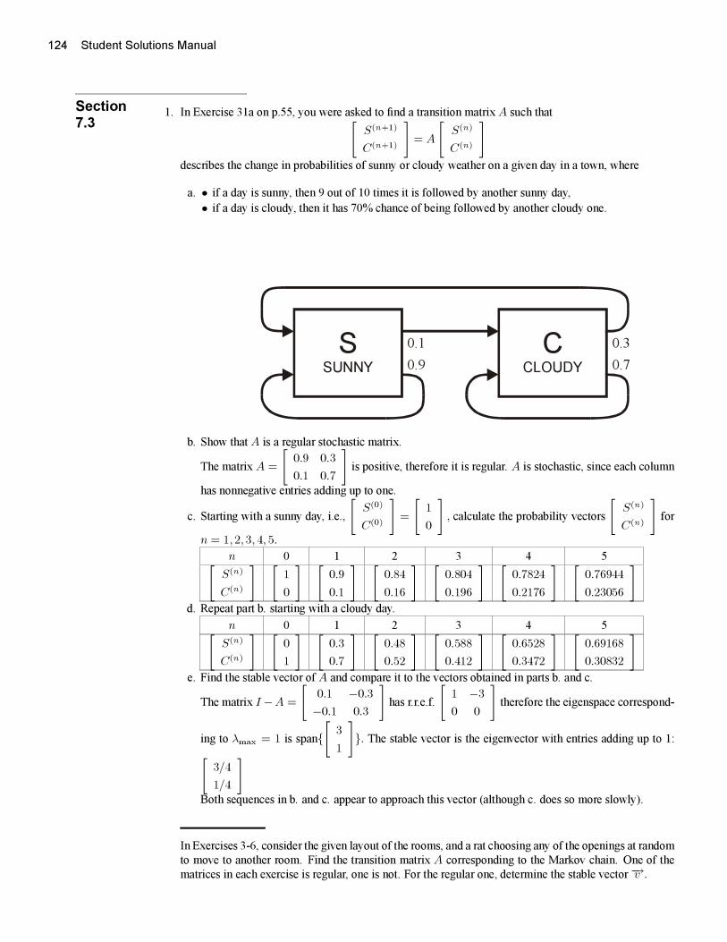
124 Student Solutions Manual
Section
7.31. In Exercise 31a on p.55, you were asked to find a transition matrix A such that[
S(n+1)
C(n+1)
]= A
[S(n)
C(n)
]describes the change in probabilities of sunny or cloudy weather on a given day in a town, where
a. • if a day is sunny, then 9 out of 10 times it is followed by another sunny day,
• if a day is cloudy, then it has 70% chance of being followed by another cloudy one.
SSUNNY
CCLOUDY0.9
0.1 0.3
0.7
b. Show that A is a regular stochastic matrix.
The matrix A =
[0.9 0.3
0.1 0.7
]is positive, therefore it is regular. A is stochastic, since each column
has nonnegative entries adding up to one.
c. Starting with a sunny day, i.e.,
[S(0)
C(0)
]=
[1
0
], calculate the probability vectors
[S(n)
C(n)
]for
n = 1,2,3, 4, 5.
n 0 1 2 3 4 5[S(n)
C(n)
] [1
0
] [0.9
0.1
] [0.84
0.16
] [0.804
0.196
] [0.7824
0.2176
] [0.76944
0.23056
]d. Repeat part b. starting with a cloudy day.
n 0 1 2 3 4 5[S(n)
C(n)
] [0
1
] [0.3
0.7
] [0.48
0.52
] [0.588
0.412
] [0.6528
0.3472
] [0.69168
0.30832
]e. Find the stable vector of A and compare it to the vectors obtained in parts b. and c.
The matrix I −A =
[0.1 −0.3
−0.1 0.3
]has r.r.e.f.
[1 −3
0 0
]therefore the eigenspace correspond-
ing to λmax = 1 is span{[
3
1
]}. The stable vector is the eigenvector with entries adding up to 1:[
3/4
1/4
]Both sequences in b. and c. appear to approach this vector (although c. does so more slowly).
In Exercises 3-6, consider the given layout of the rooms, and a rat choosing any of the openings at random
to move to another room. Find the transition matrix A corresponding to the Markov chain. One of the
matrices in each exercise is regular, one is not. For the regular one, determine the stable vector−→v .
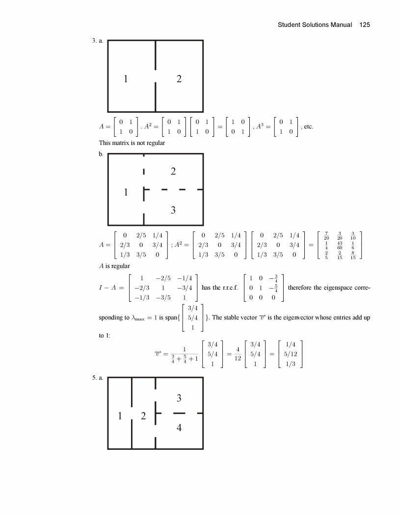
Student Solutions Manual 125
3. a.
1 2
A =
[0 1
1 0
]. A2 =
[0 1
1 0
][0 1
1 0
]=
[1 0
0 1
], A3 =
[0 1
1 0
], etc.
This matrix is not regular
b.
1
2
3
A =
⎡⎢⎣ 0 2/5 1/4
2/3 0 3/4
1/3 3/5 0
⎤⎥⎦ ; A2 =
⎡⎢⎣ 0 2/5 1/4
2/3 0 3/4
1/3 3/5 0
⎤⎥⎦⎡⎢⎣ 0 2/5 1/4
2/3 0 3/4
1/3 3/5 0
⎤⎥⎦ =
⎡⎢⎣720
320
310
14
4360
16
25
215
815
⎤⎥⎦A is regular
I − A =
⎡⎢⎣ 1 −2/5 −1/4
−2/3 1 −3/4
−1/3 −3/5 1
⎤⎥⎦ has the r.r.e.f.
⎡⎢⎣ 1 0 − 34
0 1 − 54
0 0 0
⎤⎥⎦ therefore the eigenspace corre-
sponding to λmax = 1 is span{
⎡⎢⎣ 3/4
5/4
1
⎤⎥⎦}. The stable vector−→v is the eigenvector whose entries add up
to 1:
−→v =1
34 + 5
4 +1
⎡⎢⎣ 3/4
5/4
1
⎤⎥⎦ =4
12
⎡⎢⎣ 3/4
5/4
1
⎤⎥⎦ =
⎡⎢⎣ 1/4
5/12
1/3
⎤⎥⎦5. a.
1 2
3
4
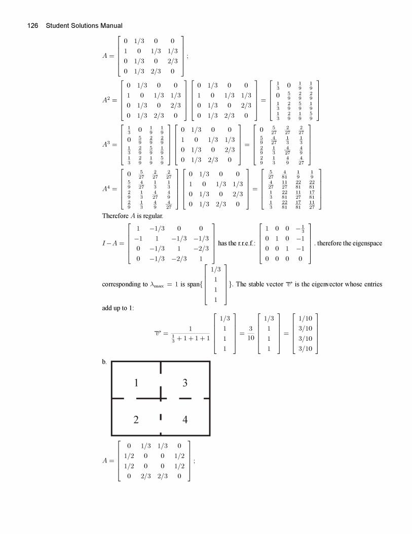
126 Student Solutions Manual
A =
⎡⎢⎢⎢⎢⎣0 1/3 0 0
1 0 1/3 1/3
0 1/3 0 2/3
0 1/3 2/3 0
⎤⎥⎥⎥⎥⎦ ;
A2 =
⎡⎢⎢⎢⎢⎣0 1/3 0 0
1 0 1/3 1/3
0 1/3 0 2/3
0 1/3 2/3 0
⎤⎥⎥⎥⎥⎦⎡⎢⎢⎢⎢⎣
0 1/3 0 0
1 0 1/3 1/3
0 1/3 0 2/3
0 1/3 2/3 0
⎤⎥⎥⎥⎥⎦ =
⎡⎢⎢⎢⎢⎣13 0 1
919
0 59
29
29
13
29
59
19
13
29
19
59
⎤⎥⎥⎥⎥⎦
A3 =
⎡⎢⎢⎢⎢⎣13 0 1
919
0 59
29
29
13
29
59
19
13
29
19
59
⎤⎥⎥⎥⎥⎦⎡⎢⎢⎢⎢⎣
0 1/3 0 0
1 0 1/3 1/3
0 1/3 0 2/3
0 1/3 2/3 0
⎤⎥⎥⎥⎥⎦ =
⎡⎢⎢⎢⎢⎣0 5
27227
227
59
427
13
13
29
13
427
49
29
13
49
427
⎤⎥⎥⎥⎥⎦
A4 =
⎡⎢⎢⎢⎢⎣0 5
27227
227
59
427
13
13
29
13
427
49
29
13
49
427
⎤⎥⎥⎥⎥⎦⎡⎢⎢⎢⎢⎣
0 1/3 0 0
1 0 1/3 1/3
0 1/3 0 2/3
0 1/3 2/3 0
⎤⎥⎥⎥⎥⎦ =
⎡⎢⎢⎢⎢⎣527
481
19
19
427
1127
2281
2281
13
2281
1127
1781
13
2281
1781
1127
⎤⎥⎥⎥⎥⎦Therefore A is regular.
I−A =
⎡⎢⎢⎢⎢⎣1 −1/3 0 0
−1 1 −1/3 −1/3
0 −1/3 1 −2/3
0 −1/3 −2/3 1
⎤⎥⎥⎥⎥⎦ has the r.r.e.f.:
⎡⎢⎢⎢⎢⎣1 0 0 −1
3
0 1 0 −1
0 0 1 −1
0 0 0 0
⎤⎥⎥⎥⎥⎦ . therefore the eigenspace
corresponding to λmax = 1 is span{
⎡⎢⎢⎢⎢⎣1/3
1
1
1
⎤⎥⎥⎥⎥⎦}. The stable vector −→v is the eigenvector whose entries
add up to 1:
−→v =1
13 + 1 + 1 + 1
⎡⎢⎢⎢⎢⎣1/3
1
1
1
⎤⎥⎥⎥⎥⎦ =3
10
⎡⎢⎢⎢⎢⎣1/3
1
1
1
⎤⎥⎥⎥⎥⎦ =
⎡⎢⎢⎢⎢⎣1/10
3/10
3/10
3/10
⎤⎥⎥⎥⎥⎦b.
1
2
3
4
A =
⎡⎢⎢⎢⎢⎣0 1/3 1/3 0
1/2 0 0 1/2
1/2 0 0 1/2
0 2/3 2/3 0
⎤⎥⎥⎥⎥⎦ ;
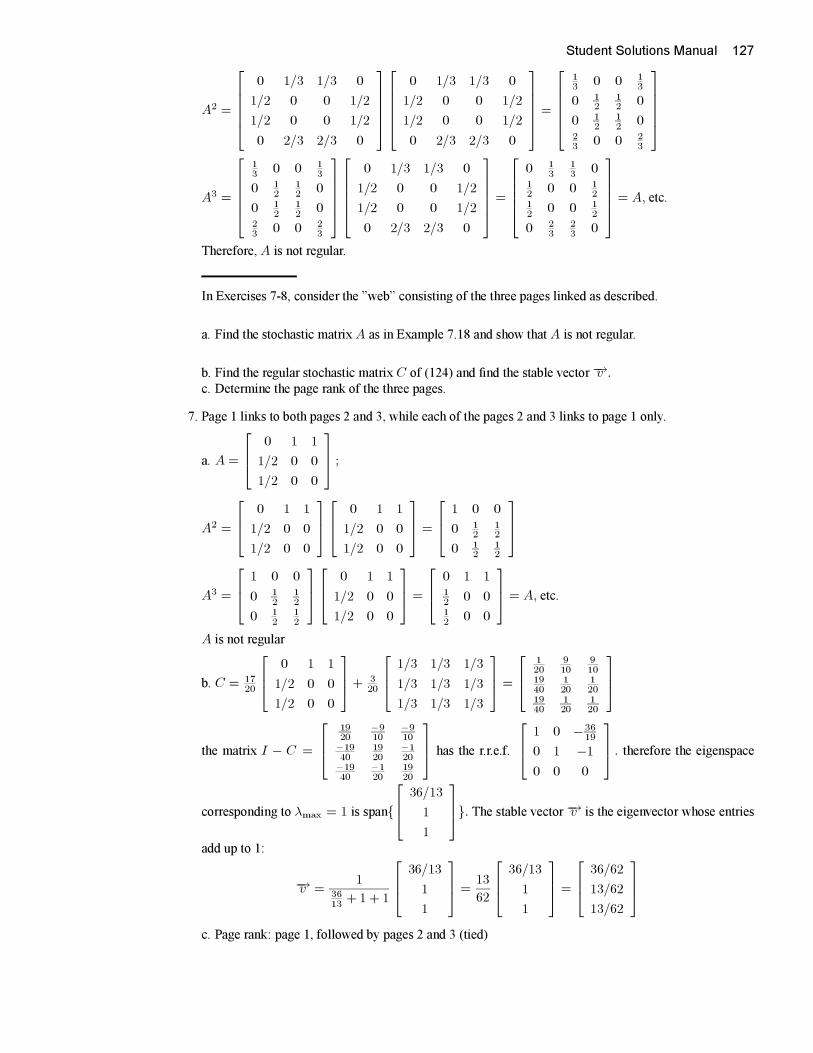
Student Solutions Manual 127
A2 =
⎡⎢⎢⎢⎢⎣0 1/3 1/3 0
1/2 0 0 1/2
1/2 0 0 1/2
0 2/3 2/3 0
⎤⎥⎥⎥⎥⎦⎡⎢⎢⎢⎢⎣
0 1/3 1/3 0
1/2 0 0 1/2
1/2 0 0 1/2
0 2/3 2/3 0
⎤⎥⎥⎥⎥⎦ =
⎡⎢⎢⎢⎢⎣13 0 0 1
3
0 12
12 0
0 12
12
023 0 0 2
3
⎤⎥⎥⎥⎥⎦
A3 =
⎡⎢⎢⎢⎢⎣13 0 0 1
3
0 12
12 0
0 12
12
023 0 0 2
3
⎤⎥⎥⎥⎥⎦⎡⎢⎢⎢⎢⎣
0 1/3 1/3 0
1/2 0 0 1/2
1/2 0 0 1/2
0 2/3 2/3 0
⎤⎥⎥⎥⎥⎦ =
⎡⎢⎢⎢⎢⎣0 1
313 0
12 0 0 1
212
0 0 12
0 23
23 0
⎤⎥⎥⎥⎥⎦ = A, etc.
Therefore,A is not regular.
In Exercises 7-8, consider the ”web” consisting of the three pages linked as described.
a. Find the stochastic matrix A as in Example 7.18 and show that A is not regular.
b. Find the regular stochastic matrix C of (124) and find the stable vector−→v .c. Determine the page rank of the three pages.
7. Page 1 links to both pages 2 and 3, while each of the pages 2 and 3 links to page 1 only.
a. A =
⎡⎢⎣ 0 1 1
1/2 0 0
1/2 0 0
⎤⎥⎦ ;
A2 =
⎡⎢⎣ 0 1 1
1/2 0 0
1/2 0 0
⎤⎥⎦⎡⎢⎣ 0 1 1
1/2 0 0
1/2 0 0
⎤⎥⎦ =
⎡⎢⎣ 1 0 0
0 12
12
0 12
12
⎤⎥⎦
A3 =
⎡⎢⎣ 1 0 0
0 12
12
0 12
12
⎤⎥⎦⎡⎢⎣ 0 1 1
1/2 0 0
1/2 0 0
⎤⎥⎦ =
⎡⎢⎣ 0 1 112 0 012 0 0
⎤⎥⎦ = A, etc.
A is not regular
b. C = 1720
⎡⎢⎣ 0 1 1
1/2 0 0
1/2 0 0
⎤⎥⎦+ 320
⎡⎢⎣ 1/3 1/3 1/3
1/3 1/3 1/3
1/3 1/3 1/3
⎤⎥⎦ =
⎡⎢⎣120
910
910
1940
120
120
1940
120
120
⎤⎥⎦
the matrix I − C =
⎡⎢⎣1920
−910
−910
−1940
1920
−120
−1940
−120
1920
⎤⎥⎦ has the r.r.e.f.
⎡⎢⎣ 1 0 −3619
0 1 −1
0 0 0
⎤⎥⎦ . therefore the eigenspace
corresponding to λmax = 1 is span{
⎡⎢⎣ 36/13
1
1
⎤⎥⎦}. The stable vector−→v is the eigenvector whose entries
add up to 1:
−→v =1
3613
+1+ 1
⎡⎢⎣ 36/13
1
1
⎤⎥⎦ =13
62
⎡⎢⎣ 36/13
1
1
⎤⎥⎦ =
⎡⎢⎣ 36/62
13/62
13/62
⎤⎥⎦c. Page rank: page 1, followed by pages 2 and 3 (tied)
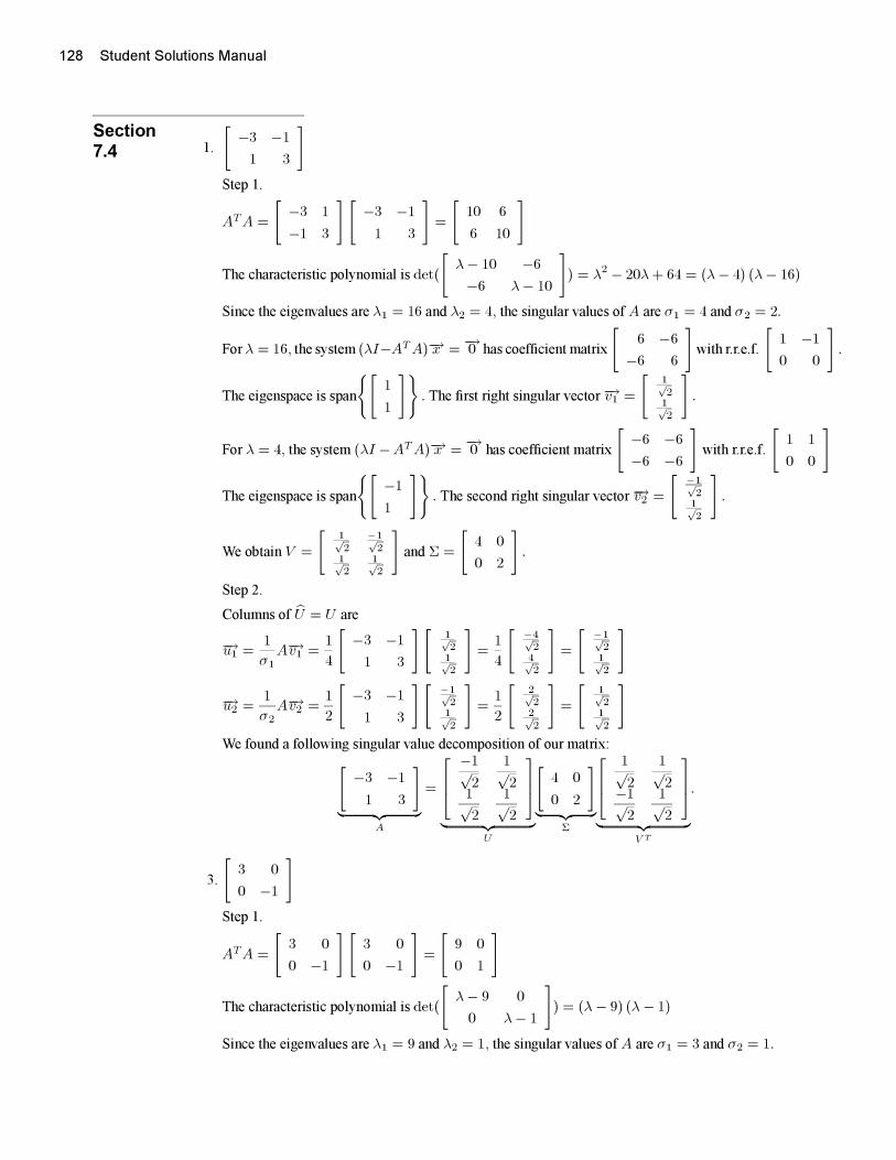
128 Student Solutions Manual
Section
7.4 1.
[−3 −1
1 3
]Step 1.
ATA =
[−3 1
−1 3
][−3 −1
1 3
]=
[10 6
6 10
]
The characteristic polynomial is det(
[λ− 10 −6
−6 λ− 10
]) = λ2 − 20λ+ 64 = (λ− 4) (λ− 16)
Since the eigenvalues are λ1 = 16 and λ2 = 4, the singular values of A are σ1 = 4 and σ2 = 2.
Forλ = 16, the system (λI−ATA)−→x =−→0 has coefficient matrix
[6 −6
−6 6
]with r.r.e.f.
[1 −1
0 0
].
The eigenspace is span
{[1
1
]}. The first right singular vector−→v1 =
[1√21√2
].
For λ = 4, the system (λI −ATA)−→x =−→0 has coefficient matrix
[−6 −6
−6 −6
]with r.r.e.f.
[1 1
0 0
]
The eigenspace is span
{[−1
1
]}. The second right singular vector−→v2 =
[ −1√21√2
].
We obtain V =
[1√2
−1√2
1√2
1√2
]and Σ =
[4 0
0 2
].
Step 2.
Columns of U = U are
−→u1 =1
σ1A−→v1 =
1
4
[−3 −1
1 3
][1√21√2
]=
1
4
[ −4√24√2
]=
[ −1√21√2
]
−→u2 =1
σ2A−→v2 =
1
2
[−3 −1
1 3
][ −1√21√2
]=
1
2
[2√22√2
]=
[1√21√2
]We found a following singular value decomposition of our matrix:[
−3 −1
1 3
]︸ ︷︷ ︸
A
=
⎡⎢⎣−1√2
1√2
1√2
1√2
⎤⎥⎦︸ ︷︷ ︸
U
[4 0
0 2
]︸ ︷︷ ︸
Σ
⎡⎢⎣1√2
1√2−1√
2
1√2
⎤⎥⎦︸ ︷︷ ︸
V T
.
3.
[3 0
0 −1
]Step 1.
ATA =
[3 0
0 −1
][3 0
0 −1
]=
[9 0
0 1
]
The characteristic polynomial is det(
[λ− 9 0
0 λ− 1
]) = (λ − 9) (λ − 1)
Since the eigenvalues are λ1 = 9 and λ2 = 1, the singular values of A are σ1 = 3 and σ2 = 1.
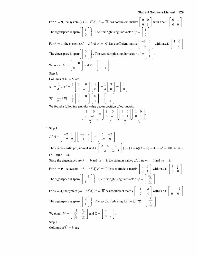
Student Solutions Manual 129
For λ = 9, the system (λI − ATA)−→x =−→0 has coefficient matrix
[0 0
0 8
]with r.r.e.f.
[0 1
0 0
].
The eigenspace is span
{[1
0
]}. The first right singular vector−→v1 =
[1
0
].
For λ = 1, the system (λI − ATA)−→x =−→0 has coefficient matrix
[−8 0
0 0
]with r.r.e.f.
[1 0
0 0
]
The eigenspace is span
{[0
1
]}. The second right singular vector−→v2 =
[0
1
].
We obtain V =
[1 0
0 1
]and Σ =
[3 0
0 1
].
Step 2.
Columns of U = U are
−→u1 =1
σ1A−→v1 =
1
3
[3 0
0 −1
] [1
0
]=
1
3
[3
0
]=
[1
0
]
−→u2 =1
σ2A−→v2 =
1
1
[3 0
0 −1
] [0
1
]=
[0
−1
]We found a following singular value decomposition of our matrix:[
3 0
0 −1
]︸ ︷︷ ︸
A
=
[1 0
0 −1
]︸ ︷︷ ︸
U
[3 0
0 1
]︸ ︷︷ ︸
Σ
[1 0
0 1
]︸ ︷︷ ︸
V T
.
5. Step 1.
ATA =
[−2 1
2 2
][−2 2
1 2
]=
[5 −2
−2 8
]
The characteristic polynomial is det(
[λ− 5 2
2 λ− 8
]) = (λ − 5)(λ − 8) − 4 = λ2 − 13λ + 36 =
(λ− 9)(λ− 4).
Since the eigenvalues are λ1 = 9 and λ2 = 4, the singular values of A are σ1 = 3 and σ2 = 2.
For λ = 9, the system (λI − ATA)−→x =−→0 has coefficient matrix
[4 2
2 1
]with r.r.e.f.
[1 1
2
0 0
].
The eigenspace is span
{[−1
2
1
]}. The first right singular vector−→v1 =
[ −1√52√5
].
Forλ = 4, the system (λI−ATA)−→x =−→0 has coefficient matrix
[−1 2
2 −4
]with r.r.e.f.
[1 −2
0 0
]
The eigenspace is span
{[2
1
]}. The second right singular vector−→v2 =
[2√51√5
].
We obtain V =
[ −1√5
2√5
2√5
1√5
]and Σ =
[3 0
0 2
].
Step 2
Columns of U = U are
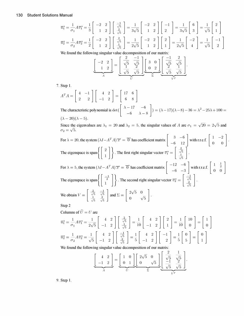
130 Student Solutions Manual
−→u1 =1
σ1A−→v1 =
1
3
[−2 2
1 2
] [ −1√52√5
]=
1
3√5
[−2 2
1 2
][−1
2
]=
1
3√5
[6
3
]=
1√5
[2
1
]
−→u2 =1
σ2A−→v2 =
1
2
[−2 2
1 2
] [2√51√5
]=
1
2√5
[−2 2
1 2
][2
1
]=
1
2√5
[−2
4
]=
1√5
[−1
2
]We found the following singular value decomposition of our matrix:[
−2 2
1 2
]︸ ︷︷ ︸
A
=
⎡⎢⎣2√5
−1√5
1√5
2√5
⎤⎥⎦︸ ︷︷ ︸
U
[3 0
0 2
]︸ ︷︷ ︸
Σ
⎡⎢⎣−1√5
2√5
2√5
1√5
⎤⎥⎦︸ ︷︷ ︸
V T
.
7. Step 1.
ATA =
[4 −1
2 2
][4 2
−1 2
]=
[17 6
6 8
]
The characteristic polynomial is det(
[λ− 17 −6
−6 λ− 8
]) = (λ−17)(λ−8)−36 = λ2−25λ+100 =
(λ− 20)(λ− 5).
Since the eigenvalues are λ1 = 20 and λ2 = 5, the singular values of A are σ1 =√20 = 2
√5 and
σ2 =√5.
Forλ = 20, the system (λI−ATA)−→x =−→0 has coefficient matrix
[3 −6
−6 12
]with r.r.e.f.
[1 −2
0 0
].
The eigenspace is span
{[2
1
]}. The first right singular vector−→v1 =
[2√51√5
].
For λ = 5, the system (λI−ATA)−→x =−→0 has coefficient matrix
[−12 −6
−6 −3
]with r.r.e.f.
[1 1
2
0 0
]
The eigenspace is span
{[−12
1
]}. The second right singular vector−→v2 =
[ −1√52√5
].
We obtain V =
[2√5
−1√5
1√5
2√5
]and Σ =
[2√5 0
0√5
].
Step 2
Columns of U = U are
−→u1 =1
σ1A−→v1 =
1
2√5
[4 2
−1 2
][2√51√5
]=
1
10
[4 2
−1 2
] [2
1
]=
1
10
[10
0
]=
[1
0
]
−→u2 =1
σ2A−→v2 =
1√5
[4 2
−1 2
][ −1√52√5
]=
1
5
[4 2
−1 2
][−1
2
]=
1
5
[0
5
]=
[0
1
]We found the following singular value decomposition of our matrix:[
4 2
−1 2
]︸ ︷︷ ︸
A
=
[1 0
0 1
]︸ ︷︷ ︸
U
[2√5 0
0√5
]︸ ︷︷ ︸
Σ
⎡⎢⎣2√5
1√5−1√
5
2√5
⎤⎥⎦︸ ︷︷ ︸
V T
.
9. Step 1.
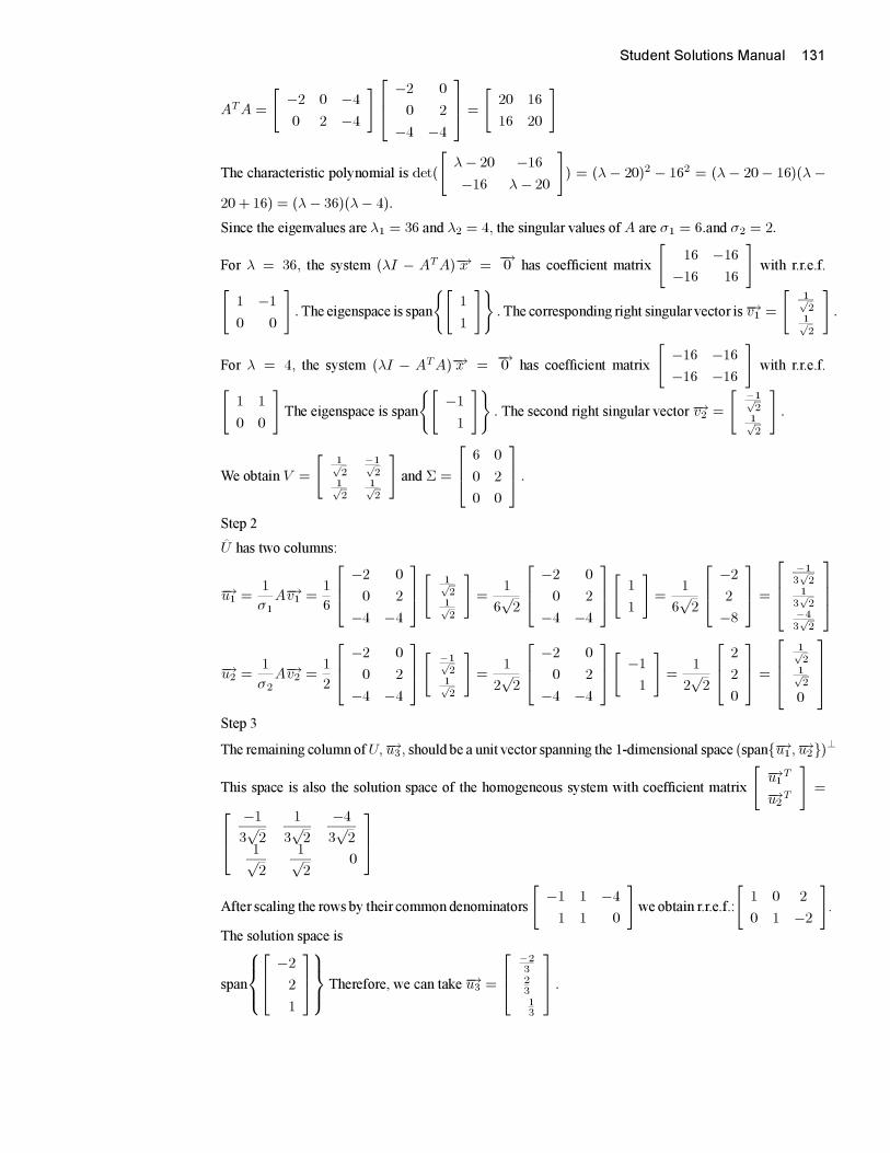
Student Solutions Manual 131
ATA =
[−2 0 −4
0 2 −4
]⎡⎢⎣ −2 0
0 2
−4 −4
⎤⎥⎦ =
[20 16
16 20
]
The characteristic polynomial is det(
[λ − 20 −16
−16 λ − 20
]) = (λ − 20)2 − 162 = (λ − 20− 16)(λ −
20 + 16) = (λ − 36)(λ− 4).
Since the eigenvalues are λ1 = 36 and λ2 = 4, the singular values of A are σ1 = 6.and σ2 = 2.
For λ = 36, the system (λI − ATA)−→x =−→0 has coefficient matrix
[16 −16
−16 16
]with r.r.e.f.[
1 −1
0 0
].The eigenspace is span
{[1
1
]}.The corresponding right singular vector is−→v1 =
[1√21√2
].
For λ = 4, the system (λI − ATA)−→x =−→0 has coefficient matrix
[−16 −16
−16 −16
]with r.r.e.f.[
1 1
0 0
]The eigenspace is span
{[−1
1
]}. The second right singular vector−→v2 =
[ −1√21√2
].
We obtain V =
[1√2
−1√2
1√2
1√2
]and Σ =
⎡⎢⎣ 6 0
0 2
0 0
⎤⎥⎦ .Step 2
U has two columns:
−→u1 =1
σ1A−→v1 =
1
6
⎡⎢⎣ −2 0
0 2
−4 −4
⎤⎥⎦[ 1√21√2
]=
1
6√2
⎡⎢⎣ −2 0
0 2
−4 −4
⎤⎥⎦[ 1
1
]=
1
6√2
⎡⎢⎣ −2
2
−8
⎤⎥⎦ =
⎡⎢⎢⎣−13√2
13√2
−43√2
⎤⎥⎥⎦−→u2 =
1
σ2A−→v2 =
1
2
⎡⎢⎣ −2 0
0 2
−4 −4
⎤⎥⎦[ −1√21√2
]=
1
2√2
⎡⎢⎣ −2 0
0 2
−4 −4
⎤⎥⎦[ −1
1
]=
1
2√2
⎡⎢⎣ 2
2
0
⎤⎥⎦ =
⎡⎢⎢⎣1√21√2
0
⎤⎥⎥⎦Step 3
The remaining column ofU,−→u3 , should be a unit vector spanning the 1-dimensional space (span{−→u1 ,−→u2})⊥
This space is also the solution space of the homogeneous system with coefficient matrix
[ −→u1T−→u2T
]=⎡⎢⎣
−1
3√2
1
3√2
−4
3√2
1√2
1√2
0
⎤⎥⎦After scaling the rows by their common denominators
[−1 1 −4
1 1 0
]we obtain r.r.e.f.:
[1 0 2
0 1 −2
].
The solution space is
span
⎧⎪⎨⎪⎩⎡⎢⎣ −2
2
1
⎤⎥⎦⎫⎪⎬⎪⎭ Therefore, we can take−→u3 =
⎡⎢⎣−232313
⎤⎥⎦ .
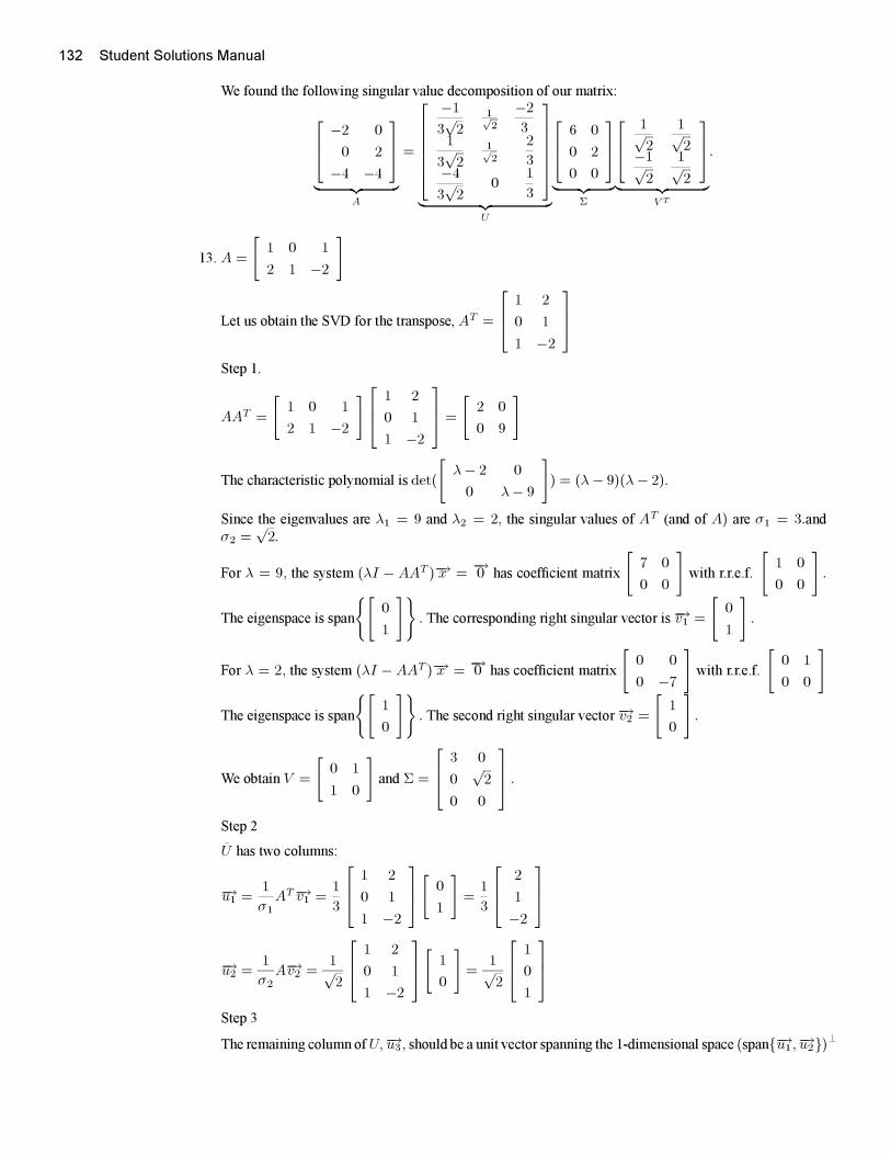
132 Student Solutions Manual
We found the following singular value decomposition of our matrix:⎡⎢⎣ −2 0
0 2
−4 −4
⎤⎥⎦︸ ︷︷ ︸
A
=
⎡⎢⎢⎢⎢⎢⎣−1
3√2
1√2
−2
31
3√2
1√2
2
3−4
3√2
01
3
⎤⎥⎥⎥⎥⎥⎦︸ ︷︷ ︸
U
⎡⎢⎣ 6 0
0 2
0 0
⎤⎥⎦︸ ︷︷ ︸
Σ
⎡⎢⎣1√2
1√2−1√
2
1√2
⎤⎥⎦︸ ︷︷ ︸
V T
.
13. A =
[1 0 1
2 1 −2
]
Let us obtain the SVD for the transpose, AT =
⎡⎢⎣ 1 2
0 1
1 −2
⎤⎥⎦Step 1.
AAT =
[1 0 1
2 1 −2
]⎡⎢⎣ 1 2
0 1
1 −2
⎤⎥⎦ =
[2 0
0 9
]
The characteristic polynomial is det(
[λ− 2 0
0 λ− 9
]) = (λ − 9)(λ − 2).
Since the eigenvalues are λ1 = 9 and λ2 = 2, the singular values of AT (and of A) are σ1 = 3.andσ2 =
√2.
For λ = 9, the system (λI − AAT )−→x =−→0 has coefficient matrix
[7 0
0 0
]with r.r.e.f.
[1 0
0 0
].
The eigenspace is span
{[0
1
]}. The corresponding right singular vector is−→v1 =
[0
1
].
For λ = 2, the system (λI − AAT )−→x =−→0 has coefficient matrix
[0 0
0 −7
]with r.r.e.f.
[0 1
0 0
]
The eigenspace is span
{[1
0
]}. The second right singular vector−→v2 =
[1
0
].
We obtain V =
[0 1
1 0
]and Σ =
⎡⎢⎣ 3 0
0√2
0 0
⎤⎥⎦ .Step 2
U has two columns:
−→u1 =1
σ1AT−→v1 =
1
3
⎡⎢⎣ 1 2
0 1
1 −2
⎤⎥⎦[ 0
1
]=
1
3
⎡⎢⎣ 2
1
−2
⎤⎥⎦−→u2 =
1
σ2A−→v2 =
1√2
⎡⎢⎣ 1 2
0 1
1 −2
⎤⎥⎦[ 1
0
]=
1√2
⎡⎢⎣ 1
0
1
⎤⎥⎦Step 3
The remaining column ofU,−→u3 , should be a unit vector spanning the 1-dimensional space (span{−→u1 ,−→u2})⊥
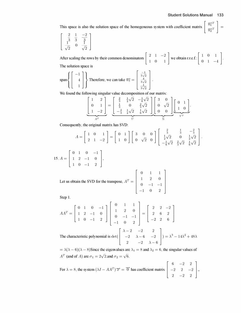
Student Solutions Manual 133
This space is also the solution space of the homogeneous system with coefficient matrix
[ −→u1T−→u2T
]=⎡⎢⎣ 2
3
1
3
−2
31√2
01√2
⎤⎥⎦After scaling the rows by their common denominators
[2 1 −2
1 0 1
]we obtain r.r.e.f.:
[1 0 1
0 1 −4
].
The solution space is
span
⎧⎪⎨⎪⎩⎡⎢⎣ −1
4
1
⎤⎥⎦⎫⎪⎬⎪⎭ Therefore, we can take−→u3 =
⎡⎢⎢⎣−13√2
43√2
13√2
⎤⎥⎥⎦ .We found the following singular value decomposition of our matrix:⎡⎢⎣ 1 2
0 1
1 −2
⎤⎥⎦︸ ︷︷ ︸
AT
=
⎡⎢⎣23
12
√2 −1
6
√2
13 0 2
3
√2
− 23
12
√2 1
6
√2
⎤⎥⎦︸ ︷︷ ︸
U
⎡⎢⎣ 3 0
0√2
0 0
⎤⎥⎦︸ ︷︷ ︸
Σ
[0 1
1 0
]︸ ︷︷ ︸
V T
.
Consequently, the original matrix has SVD:
A =
[1 0 1
2 1 −2
]=
[0 1
1 0
][3 0 0
0√2 0
]⎡⎢⎣23
13 −2
312
√2 0 1
2
√2
− 16
√2 2
3
√2 1
6
√2
⎤⎥⎦ .
15. A =
⎡⎢⎣ 0 1 0 −1
1 2 −1 0
1 0 −1 2
⎤⎥⎦,
Let us obtain the SVD for the transpose, AT =
⎡⎢⎢⎢⎢⎣0 1 1
1 2 0
0 −1 −1
−1 0 2
⎤⎥⎥⎥⎥⎦Step 1.
AAT =
⎡⎢⎣ 0 1 0 −1
1 2 −1 0
1 0 −1 2
⎤⎥⎦⎡⎢⎢⎢⎢⎣
0 1 1
1 2 0
0 −1 −1
−1 0 2
⎤⎥⎥⎥⎥⎦ =
⎡⎢⎣ 2 2 −2
2 6 2
−2 2 6
⎤⎥⎦
The characteristic polynomial is det(
⎡⎢⎣ λ − 2 −2 2
−2 λ− 6 −2
2 −2 λ− 6
⎤⎥⎦) = λ3 − 14λ2 + 48λ
= λ(λ − 6)(λ − 8)Since the eigenvalues are λ1 = 8 and λ2 = 6, the singular values of
AT (and of A) are σ1 = 2√2.and σ2 =
√6.
For λ = 8, the system (λI −AAT )−→x =−→0 has coefficient matrix
⎡⎢⎣ 6 −2 2
−2 2 −2
2 −2 2
⎤⎥⎦„
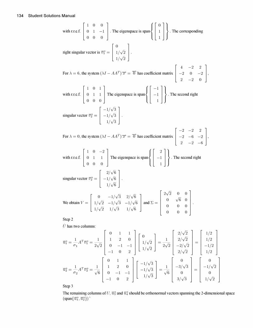
134 Student Solutions Manual
with r.r.e.f.
⎡⎢⎣ 1 0 0
0 1 −1
0 0 0
⎤⎥⎦ . The eigenspace is span⎧⎪⎨⎪⎩⎡⎢⎣ 0
1
1
⎤⎥⎦⎫⎪⎬⎪⎭ . The corresponding
right singular vector is−→v1 =
⎡⎢⎣ 0
1/√2
1/√2
⎤⎥⎦ .
For λ = 6, the system (λI −AAT )−→x =−→0 has coefficient matrix
⎡⎢⎣ 4 −2 2
−2 0 −2
2 −2 0
⎤⎥⎦,
with r.r.e.f.
⎡⎢⎣ 1 0 1
0 1 1
0 0 0
⎤⎥⎦ The eigenspace is span
⎧⎪⎨⎪⎩⎡⎢⎣ −1
−1
1
⎤⎥⎦⎫⎪⎬⎪⎭ . The second right
singular vector −→v2 =
⎡⎢⎣ −1/√3
−1/√3
1/√3
⎤⎥⎦ .
For λ = 0, the system (λI −AAT )−→x =−→0 has coefficient matrix
⎡⎢⎣ −2 −2 2
−2 −6 −2
2 −2 −6
⎤⎥⎦,
with r.r.e.f.
⎡⎢⎣ 1 0 −2
0 1 1
0 0 0
⎤⎥⎦ The eigenspace is span
⎧⎪⎨⎪⎩⎡⎢⎣ 2
−1
1
⎤⎥⎦⎫⎪⎬⎪⎭ . The second right
singular vector −→v2 =
⎡⎢⎣ 2/√6
−1/√6
1/√6
⎤⎥⎦ .
We obtain V =
⎡⎢⎣ 0 −1/√3 2/
√6
1/√2 −1/
√3 −1/
√6
1/√2 1/
√3 1/
√6
⎤⎥⎦ and Σ =
⎡⎢⎢⎢⎢⎣2√2 0 0
0√6 0
0 0 0
0 0 0
⎤⎥⎥⎥⎥⎦ .Step 2
U has two columns:
−→u1 =1
σ1AT−→v1 =
1
2√2
⎡⎢⎢⎢⎢⎣0 1 1
1 2 0
0 −1 −1
−1 0 2
⎤⎥⎥⎥⎥⎦⎡⎢⎣ 0
1/√2
1/√2
⎤⎥⎦ =1
2√2
⎡⎢⎢⎢⎢⎣2/
√2
2/√2
−2/√2
2/√2
⎤⎥⎥⎥⎥⎦ =
⎡⎢⎢⎢⎢⎣1/2
1/2
−1/2
1/2
⎤⎥⎥⎥⎥⎦
−→u2 =1
σ2AT−→v2 =
1√6
⎡⎢⎢⎢⎢⎣0 1 1
1 2 0
0 −1 −1
−1 0 2
⎤⎥⎥⎥⎥⎦⎡⎢⎣ −1/
√3
−1/√3
1/√3
⎤⎥⎦ =1√6
⎡⎢⎢⎢⎢⎣0
−3/√3
0
3/√3
⎤⎥⎥⎥⎥⎦ =
⎡⎢⎢⎢⎢⎣0
−1/√2
0
1/√2
⎤⎥⎥⎥⎥⎦Step 3
The remaining columns of U,−→u3 and−→u4 should be orthonormal vectors spanning the 2-dimensional space
(span{−→u1 ,−→u2})⊥
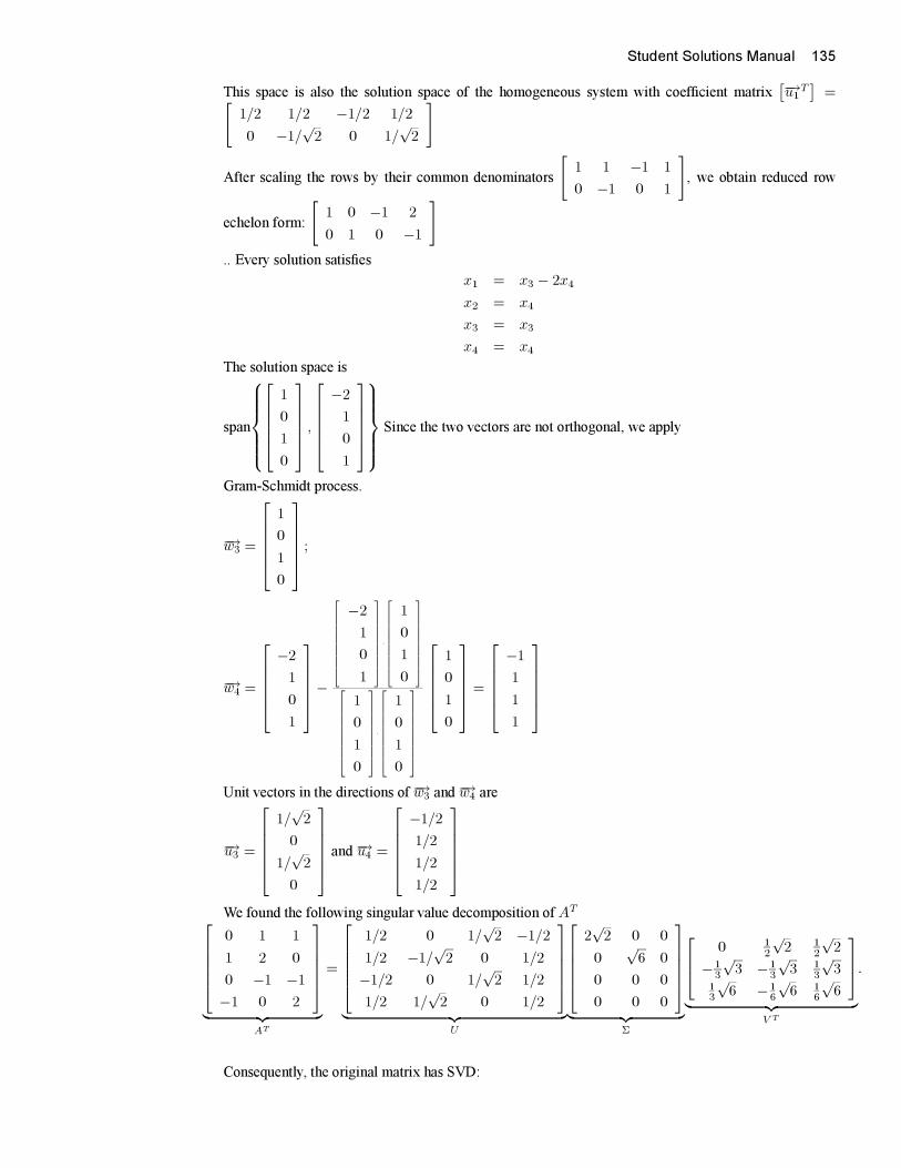
Student Solutions Manual 135
This space is also the solution space of the homogeneous system with coefficient matrix[−→u1
T]
=[1/2 1/2 −1/2 1/2
0 −1/√2 0 1/
√2
]
After scaling the rows by their common denominators
[1 1 −1 1
0 −1 0 1
], we obtain reduced row
echelon form:
[1 0 −1 2
0 1 0 −1
].. Every solution satisfies
x1 = x3 − 2x4
x2 = x4
x3 = x3
x4 = x4The solution space is
span
⎧⎪⎪⎪⎪⎨⎪⎪⎪⎪⎩
⎡⎢⎢⎢⎢⎣1
0
1
0
⎤⎥⎥⎥⎥⎦ ,⎡⎢⎢⎢⎢⎣
−2
1
0
1
⎤⎥⎥⎥⎥⎦⎫⎪⎪⎪⎪⎬⎪⎪⎪⎪⎭ Since the two vectors are not orthogonal, we apply
Gram-Schmidt process.
−→w3 =
⎡⎢⎢⎢⎢⎣1
0
1
0
⎤⎥⎥⎥⎥⎦ ;
−→w4 =
⎡⎢⎢⎢⎢⎣−2
1
0
1
⎤⎥⎥⎥⎥⎦−
⎡⎢⎢⎢⎢⎢⎢⎢⎢⎣
−2
1
0
1
⎤⎥⎥⎥⎥⎥⎥⎥⎥⎦·
⎡⎢⎢⎢⎢⎢⎢⎢⎢⎣
1
0
1
0
⎤⎥⎥⎥⎥⎥⎥⎥⎥⎦
⎡⎢⎢⎢⎢⎢⎢⎢⎢⎣
1
0
1
0
⎤⎥⎥⎥⎥⎥⎥⎥⎥⎦·
⎡⎢⎢⎢⎢⎢⎢⎢⎢⎣
1
0
1
0
⎤⎥⎥⎥⎥⎥⎥⎥⎥⎦
⎡⎢⎢⎢⎢⎣1
0
1
0
⎤⎥⎥⎥⎥⎦ =
⎡⎢⎢⎢⎢⎣−1
1
1
1
⎤⎥⎥⎥⎥⎦
Unit vectors in the directions of −→w3 and−→w4 are
−→u3 =
⎡⎢⎢⎢⎢⎣1/√2
0
1/√2
0
⎤⎥⎥⎥⎥⎦ and −→u4 =
⎡⎢⎢⎢⎢⎣−1/2
1/2
1/2
1/2
⎤⎥⎥⎥⎥⎦We found the following singular value decomposition of AT⎡⎢⎢⎢⎢⎣0 1 1
1 2 0
0 −1 −1
−1 0 2
⎤⎥⎥⎥⎥⎦︸ ︷︷ ︸
AT
=
⎡⎢⎢⎢⎢⎣1/2 0 1/
√2 −1/2
1/2 −1/√2 0 1/2
−1/2 0 1/√2 1/2
1/2 1/√2 0 1/2
⎤⎥⎥⎥⎥⎦︸ ︷︷ ︸
U
⎡⎢⎢⎢⎢⎣2√2 0 0
0√6 0
0 0 0
0 0 0
⎤⎥⎥⎥⎥⎦︸ ︷︷ ︸
Σ
⎡⎢⎣ 0 12
√2 1
2
√2
−13
√3 −1
3
√3 1
3
√3
13
√6 −1
6
√6 1
6
√6
⎤⎥⎦︸ ︷︷ ︸
V T
.
Consequently, the original matrix has SVD:
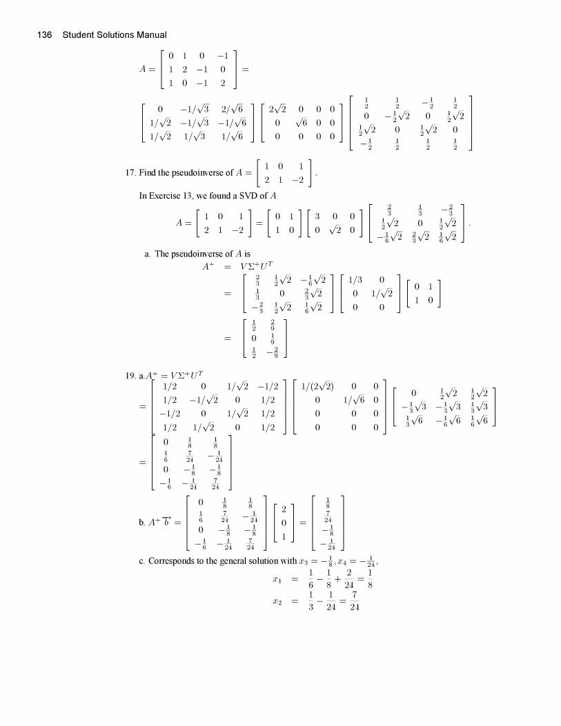
136 Student Solutions Manual
A =
⎡⎢⎣ 0 1 0 −1
1 2 −1 0
1 0 −1 2
⎤⎥⎦ =
⎡⎢⎣ 0 −1/√3 2/
√6
1/√2 −1/
√3 −1/
√6
1/√2 1/
√3 1/
√6
⎤⎥⎦⎡⎢⎣ 2
√2 0 0 0
0√6 0 0
0 0 0 0
⎤⎥⎦⎡⎢⎢⎢⎢⎣
12
12
−12
12
0 −12
√2 0 1
2
√2
12
√2 0 1
2
√2 0
−12
12
12
12
⎤⎥⎥⎥⎥⎦17. Find the pseudoinverse of A =
[1 0 1
2 1 −2
].
In Exercise 13, we found a SVD of A
A =
[1 0 1
2 1 −2
]=
[0 1
1 0
][3 0 0
0√2 0
]⎡⎢⎣23
13
−23
12
√2 0 1
2
√2
− 16
√2 2
3
√2 1
6
√2
⎤⎥⎦ .a. The pseudoinverse of A is
A+ = V Σ+UT
=
⎡⎢⎣23
12
√2 −1
6
√2
13
0 23
√2
−23
12
√2 1
6
√2
⎤⎥⎦⎡⎢⎣ 1/3 0
0 1/√2
0 0
⎤⎥⎦[ 0 1
1 0
]
=
⎡⎢⎣12
29
0 19
12 −2
9
⎤⎥⎦19. a.A+ = V Σ+UT
=
⎡⎢⎢⎢⎢⎣1/2 0 1/
√2 −1/2
1/2 −1/√2 0 1/2
−1/2 0 1/√2 1/2
1/2 1/√2 0 1/2
⎤⎥⎥⎥⎥⎦⎡⎢⎢⎢⎢⎣
1/(2√2) 0 0
0 1/√6 0
0 0 0
0 0 0
⎤⎥⎥⎥⎥⎦⎡⎢⎣ 0 1
2
√2 1
2
√2
−13
√3 −1
3
√3 1
3
√3
13
√6 −1
6
√6 1
6
√6
⎤⎥⎦
=
⎡⎢⎢⎢⎢⎣0 1
818
16
724
− 124
0 −18 −1
8
−16 − 1
24724
⎤⎥⎥⎥⎥⎦
b. A+−→b =
⎡⎢⎢⎢⎢⎣0 1
818
16
724
− 124
0 − 18 − 1
8
−16 − 1
24724
⎤⎥⎥⎥⎥⎦⎡⎢⎣ 2
0
1
⎤⎥⎦ =
⎡⎢⎢⎢⎢⎣18724
− 18
− 124
⎤⎥⎥⎥⎥⎦c. Corresponds to the general solution with x3 = −1
8 , x4 = − 124 ,
x1 =1
6− 1
8+
2
24=
1
8
x2 =1
3− 1
24=
7
24