STRUCTURED POPULATION MODELS

Can subdivide populations by:

• where individuals occur in space (e.g. metapopulation models)

• the age of individuals (age-structured models)

• the size of individuals (size-structured models)

• the stage of individuals (stage-structured individuals)

Life cycle of a fir

Sexual adult

larvae,1st instar

egg

pupae

larvae,3rd instar

larvae,2nd instar

oviposition

1st molt

2nd molt

hatching

diapause, pupation

emergence

Fecundity schedules:

average fertility of females a function of their ages.

Survivorship schedules:

average mortality rates as a function of age.

Fecundity schedules:Semelparous (in animals) or monocarpic (in plants) reproduction:

when organisms reproduce only once in their lifetime.

Iteroparous (in animals) or polycarpic (in plants) reproduction:when organisms reproduce more than once in their lifetime.

Marine salmon Century plant

Elephant Cherry tree

Survivorship schedules:

In plants we distinguish: annuals, biennials, perennials.

An annual: sunflower

A biennial: spinach

A perennial: sequoia

Age

ln S

urvi

vors

hip

Type I: mammals with much parental care in a low risk environment.

Three types of survivorship curves:

Type II: (rare) Individuals of all ages have the same probability of dying.

Type III: Species with many, small and vulnerable young.

This is equivalent to exponential decay:

constant mortality risk throughout a lifetime

To develop an age-structured model:

1. Partition the population into age classes (N1(t), N2(t),….)

2. Formulate rules of transition from one age class into the next.

3. Use probabilities of survival from one age class to the next Pi

4. Use age specific fecundities Fi

Book keeping: (assuming birth-pulse model & post-breeding census)

Life historyinterval

Age (x) x = 1 x = 4x = 3x = 2 x = 5x=0

BIRTH DEATH OF OLDEST INDIVIDUAL

S(0) S(1) S(2) S(3) S(4) S(5) = 0

S(x): the number of survivors at the beginning of age x

b(1) b(2)

b(x): the per-capita birth rate for members of the age class x

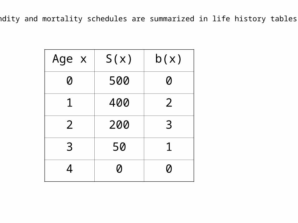
Fecundity and mortality schedules are summarized in life history tables:

Age x S(x) b(x)

0 500 0

1 400 2

2 200 3

3 50 1

4 0 0

Estimate model parameters from table:

Age x S(x) b(x) l(x) Pi Fi

0 500 0 1

1 400 2 0.8 0.8 1.60

2 200 3 0.4 0.5 1.50

3 50 1 0.1 0.25 0.25

4 0 0 0.0 0.0 0.00

)(0.0)1(

)(25.0)1(

)(5.0)1(

)(8.0)1(

)(25.0)(5.1)(6.1)1(

45

34

23

12

3211

tNtN

tNtN

tNtN

tNtN

tNtNtNtN

...

...

)()1(

)()1(

)()1(

...)()()()1(

334

223

112

3322111

tNptN

tNptN

tNptN

tNftNftNftN

Generalized:

In Matrix form:

)1(

)1(

)1(

)1(

4

3

2

1

tN

tN

tN

tN

000

000

000

3

2

1

4321

p

p

p

ffff

)(

)(

)(

)(

4

3

2

1

tN

tN

tN

tN

=

Leslie Matrix

n(t+1) = A n(t)

Asymptotic behavior:Linear model: no equilibrium points except zero.Exponential decline or increase.One form of asymptotic behavior are stable age distributions:

Any study that does not address asymptotic analysis, transient analysis, ergodicity (dependence of asymptotic behavior on initial conditions) and the results of perturbations has not completely explored its model. -Hal Caswell in Matrix Population Models (2001)

n(t+1) = n(t)

n(t+1) = A n(t)

Where n(t) and n(t+1) are in stable age distribution (where the proportion of individuals in the age classes does not change) and is the asymptotic exponential growth rate.

In Matrix algebra, in the formula (not zero):

A n(t) = n(t)

is called the eigenvalue of a matrixn(t) is called the eigenvector of a matrix

Solving for the eigenvalue and eigenvector involves solving:

(A - I)n(t) = 0

Where I is the Identity Matrix, a square matrix with 1’s in the diagonal and 0’s everywhere else.

Simple example:

N1(t+1) = 3.0 N2(t) +N3(t)

N2(t+1) = 0.3 N1(t)

N3(t+1) = 0.5N2(t)

Generalizations:

1. There are as many eigenvalues as there are numbers of equations (unless the matrix is reducible).

2. The asymptotic behavior of the model is determines by the dominant eigenvalue 1, which is the eigenvalue with the largest absolute number.

3. The population grows if 1>1, shrinks if 1<1.

Projection matrices can be visualized in “digraphs”, where every age/stage isrepresented by a symbol and every transition by an arrow. For example:

000

000

000

0

3

2

1

432

p

p

p

fff

1 2 3 4p1 p3p2

f2

f4f3

Some more generalizations:

If there is a path from every stage to every other stage, thematrix is irreducible. – The model cannot be reduced to a simpler model.

Reducibility:

Every irreducible, nonnegative matrix has a real, positive dominant eigenvalue and a real positive eigenvector. (Perron-Frobenius theorem)

1 2 3 4p1 p3p2

f2

f4f3

Irreducible:

1 2 3 4p1 p3p2

f2

f3

Reducible:

A nonnegative irreducible matrix is primitive if and only if the greatest common divisor of all circuit lengths is 1.

Primitivity:

1 2 3p1 p2

f2

f1

f3

This matrix has 3 circuits of lengths 1, 2, and 3. The greatest common divisor is 1. The matrix is primitive.

f4

1 2 3p1 p2

f3

4p3

This matrix has 2 circuits of lengths 2 and 4. The greatest common divisor is 2. The matrix is imprimitive.

Imprimitive matrices cycle. They have complex eigenvalues and do not converge on a stable age distribution. They have real, positive eigenvectors.