Embed Size (px)
Citation preview

SEASONAL INFLUENCE ON AGE-STRUCTURED INVASIVESPECIES WITH YEARLY GENERATION
YINGLI PAN∗, JIAN FANG† , AND JUNJIE WEI‡
Abstract. How do seasonal successions influence the propagation dynamics of an age-structuredinvasive species? We investigate this problem by considering the scenario that the offsprings arereproduced in spring and then reach maturation in fall within the same year. For this purpose, areaction-diffusion system is proposed, with yearly periodic time delay and spatially nonlocal responsecaused by the periodic developmental process. By appealing to the recently developed dynamicalsystem theories, we obtain the invasion speed c∗ and its coincidence with the minimal speed of timeperiodic traveling waves. The characterizations of c∗ suggest that (i) time delay decreases the speedand its periodicity may further do so; (ii) the optimal time to slow down the invasion is the seasonwithout juveniles; (iii) the speed increases to infinity with the same order as the square root of thediffusion rate.
Key words. Periodic delay; Seasonal influence; Invasion speed; Traveling wave.
AMS subject classifications. Primary: 92D25; Secondary: 34K13, 35C07, 37N25
1. Introduction. Seasonal successions bring invasive species temporally dy-namic habitats, which then affect their life cycles, including breeding, development,mobility, maturation, mortality, etc, and further give rise to the propagation complex-ity during their invasion process. How seasonality influences the propagation of anage-structured invasive species is a challenging problem from the viewpoints of bothmathematical modeling and analysis.
In this paper, we intend to investigate such a problem for a single invasive speciesby considering the scenario that the species has distinct breeding and maturationseasons. More precisely, we assume that the species has the following biological char-acteristics.
(B1) The species can be classified into two stages by age: mature and immature.An individual at time t belongs to the mature class if and only if its ageexceeds the time dependent positive number τ(t). Within each stage, allindividuals share the same behavior.
(B2) Adults reproduce offsprings once a year in a fixed season (spring), and theyreach maturation in another season (fall) within the same year.
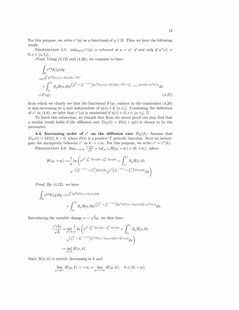
(B3) All behaviors are yearly periodic due to seasonal succession.(B4) The spatial habitat is ideally assumed to be one dimensional and homogeneous
in locations.We refer to Fig. 1.1 for a schematic illustration of the life cycle in a year [0, T ]. Sincethe habitat is dynamic in time, the biological developmental rate of species may bedifferent from one time to another. So we assume that the duration τ = τ(t) fromnewborn to being adult is yearly time periodic. Further, since the developmental ratedepends only on time, juveniles cannot reach maturation before those born ahead ofthem. Therefore, one has following additional implicit assumption.
(B5) t− τ(t) is strictly increasing in t, that is, τ ′(t) < 1 if τ is a smooth function.
∗Department of Mathematics, Harbin Institute of Technology, Harbin, Heilongjiang, 150001,China ([email protected])†Institute for Advanced Studies in Mathematics and Department of Mathematics, Harbin Institute
of Technology, Harbin, Heilongjiang, 150001, China ([email protected])‡School of Science, Harbin Institute of Technology in Weihai, Weihai, Shandong, 264209, China
1
arX
iv:1
712.
0624
1v1
[m
ath.
AP]
18
Dec
201
7

2
0 T t t
Breeding period Maturation period
( )t
t( )t t
Fig. 1.1. Schematic illustrations of the life cycle for the species with yearly generation, where[α, β] is the breeding period and [tα, tβ ] is the maturation period.
To mathematically model such an invasive species, we start from the followinggrowth law for two stages of age-structured population (see Metz and Diekmann [14]):
(∂
∂t+
∂
∂a
)p = DM (t)
∂2
∂x2p− dM (t)p, a ≥ τ(t)(
∂
∂t+
∂
∂a
)p = DI(t)
∂2
∂x2p− dI(t)p, 0 < a < τ(t),
t > 0, x ∈ R, (1.1)
where p = p(x, t, a) denotes the density of species of age a at time t and locationx, DM , DI are the diffusion rates, and dM , dI are the death rates. Clearly, the totalmature population u and immature population v at time t and location x can berepresented, respectively, by the integrals
u(t, x) =
∫ +∞
τ(t)
p(x, t, a)da, v(t, x) =
∫ τ(t)
0
p(x, t, a)da.
Keeping a smooth flow for the paper, we write down here the model while leavingin the next section the derivation details, which are highly motivated by the ideasbehind a few recent works. We will explain the details in the next few paragraphs.
∂u
∂t= DM (t)
∂2u
∂x2− dM (t)u+R(t, u(t− τ(t), ·))(x),
∂v
∂t= DI(t)
∂2v
∂x2− dI(t)v + b(t, u(x, t))−R(t, u(t− τ(t), ·))(x),
t > 0, x ∈ R,
(1.2)where R in general is a nonlocal term, meaning the recruitment rate of mature pop-ulation at time t and location x, and function b is the birth rate. The recruitmentterm R turns out to have the following expression
R(t, φ)(x) = (1− τ ′(t))b(t− τ(t), φ) ∗ kI(t, t− τ(t), ·)(x), (1.3)
where
kI(t, t− τ(t), x) =ε(t)√4πσ(t)
exp
− x2
4σ(t)
=: ε(t)fσ(t)(x) (1.4)
is the Green function of ∂tρ = DI(t)∂xx − dI(t), x ∈ R. Assumption (B5), i.e.,τ ′(t) < 1, ensures the positivity and well-posedness of the recruitment term, in which,(1− τ ′(t))ε(t) is the survival rate from newborn to being adult, fσ(t) is the redistribu-tion kernel in space for newborns upon they become mature, and σ(t), derived from

3
the diffusion of immature population, measures how strong the nonlocal interaction(induced by the diffusibility of immature population) is.
Let us recall some related works that motivate our study. In a pioneer paper onperiodic delays, Freedman and Wu [4] studied the existence of a periodic solution ofa single species population model
u′(t) = u(t)[a(t)− b(t)u(t) + c(t)u(t− τ(t))], (1.5)
where the positive functions a, b, c, τ are all ω-periodic for some ω > 0. Li andKuang [8] investigated a two species Lotka-Volterra model with distributed periodicdelays. Recently, an increasing attention has been paid to the emerging term 1−τ ′(t)in modeling the periodic/state-dependent development for juveniles. We refer toBarbarossa et al. [1], Wu et al. [20] and Kloosterman et al. [7] for the biologicalmeanings in various scenarios. Very recently, the basic reproduction number theoryhas been developed by Lou and Zhao [13] for a large class of disease models withperiodic delays, by employing which Wang and Zhao [18] analyzed a malaria modelwith temperature-dependent incubation period and Liu et al. [12] analyzed a tickpopulation model subject to seasonal effects.
By considering a single invasive species with two stages distinguished by age, Soet al. [16] formulated a reaction-diffusion model in R with constant time delay andspatially nonlocal interaction
∂tu = ∂xxu− du+ e−γτ b(u(t− τ, ·)) ∗ kσ(τ), x ∈ R, (1.6)
where u represents the density of mature population, the positive constant τ is thematuration period, and the whole nonlocal term is the recruitment of mature popu-lation, accounting for the redistribution of survived juveniles at the time when theyreach maturation. Such a mechanism generating nonlocal term has stimulated manydevelopments in differential equations, dynamical systems and nonlinear analysis [5].Under suitable conditions, it has been shown in [10] that the invasion speed c∗ coin-cides with the minimal speed of traveling waves that is determined by the variational
formula c∗ = infµ>0λ(µ)µ , where λ(µ) is the principal eigenvalue of
λ = µ2 − d+ e−γτ b′(0)kσ(τ) ∗ e−λ(τ+·). (1.7)
It is proved by Li et al. [9] that c∗ is decreasing in delay τ (see also [17]).With the aforementioned works, a natural question then arises: what if the peri-
odic development rate is incorporated into the population model (1.6)? Further, howdoes the periodicity affect the invasion speed c∗? For this purpose, we proposed themodel (1.2), which is a generalized version of (1.6).
If assuming all time periodic parameters are constants in (1.2), then one mayretrieve (1.6). If assuming only delay is a constant, then one has the model studiedby Jin and Zhao [6]. If assuming that the mobility of immature population can beignored, i.e., passing σ(t)→ 0, then one can see that fσ(t) tends to the Dirac measureand the nonlocal term R reduces to the local form
(1− τ ′(t))ε(t)b(t− τ(t), u(t− τ(t), x)). (1.8)
If assuming the mobility of mature population can be ignored, i.e., DM (t) ≡ 0, thenone has the following integro-differential equation for the mature population:
∂u(t, x)
∂t= −dM (t)u(t, x) +R(t, u(t− τ(t), ·))(x), (1.9)

4
which looks simpler than the diffusive equation but has more mathematical challengesdue to the lack of regularity in spatial variable x.
Clearly, model (1.2) is partially uncoupled. But it is still hard to fully under-stand how the time heterogeneity influences the propagation dynamics, especiallythe periodicity of time delay. In virtue of biological assumption (B2), we may castthe first equation of model (1.2) for the mature population into an iterative systemdetermined by its Poincare map. This feature will be essentially of help for the math-ematical analysis. As for the immature population, the second equation in model(1.2) can be regarded as a linear time periodic reaction-diffusion equation with aninhomogeneous reaction term once the invasion of mature population is understood.To analyze such an equation, the following conservation equality will play an vitalrole. It comes from the biological observation that all newborns will become maturein the same year as when they were born.
∫ T
0
kI(t, s, ·) ∗ b(s, u(s, ·))ds =
∫ T
0
kI(t, s, ·) ∗R(s, u(s− τ(s), ·))ds, t > T, (1.10)
where kI(t, s, x) is the Green function of ∂tρ = DI(t)∂xxρ− dI(t)ρ.The rest of this paper is organized as follows. In section 2, we formulate the model
(1.2) and reduce its first equation to the iterative system (2.12)-(2.14). In section 3, weinvestigate the global dynamics for the spatially homogeneous system of (2.12)-(2.14).In section 4, we first employ the dynamical system theories in [3, 11, 10, 19] to obtainthe invasion speed c∗ and its coincidence with the minimal speed of traveling waves,and then we investigate the parameter influence on c∗, including the time periodicity.In the last section, we are back to model (1.2) and establish the propagation dynamicswith the help of (1.10).
2. Model. In this section, we first formulate the reaction-diffusion model system(1.2) from the growth law (1.1) and then reduce it to the iterative system (2.12)-(2.14)by using the biological characteristics as assumed in the previous section.
2.1. Reaction-diffusion model with periodic delay. Let p(t, x, a) denotethe population density of the species under consideration at time t ≥ 0, age a ≥ 0and location x ∈ R. According to assumption (B1), the total matured population attime t and location x is given by
u(t, x) =
∫ +∞
τ(t)
p(t, x, a)da. (2.1)
It is natural to assume that p(t, x,+∞) = 0. Differentiating the both sides of (2.1)in time yields
∂
∂tu(t, x) =
∫ ∞τ(t)
∂
∂tp(t, x, a)da− τ ′(t)p(t, x, τ(t)). (2.2)
By using the growth law (1.1), we obtain that∫ ∞τ(t)
∂
∂tp(t, x, a)da=
∫ ∞τ(t)
[− ∂
∂a+DM (t)
∂2
∂x2− dM (t)
]p(t, x, a)da
= DM (t)∂2
∂x2u(t, x)− dM (t)u(t, x) + p(t, x, τ(t)). (2.3)

5
Consequently, (2.2) becomes
∂
∂tu(t, x) = DM (t)
∂2
∂x2u(t, x)− dM (t)u(t, x) + (1− τ ′(t))p(t, x, τ(t)). (2.4)
To obtain a closed form of the model, one needs to express p(t, x, τ(t)) by u in acertain way. Indeed, p(t, x, τ(t)) represents the newly matured population at time t,and it is the evolution result of newborns at t − τ(t). That is, there is an evolutionrelation between the quantities p(t, x, τ(t)) and p(t − τ(t), x, 0). Such a relation isobeyed by the second equation of the growth law (1.1). More precisely, the relationis the time-τ(t) solution map of the following evolution equation
∂q
∂s= DI(t− τ(t) + s)
∂2q
∂x2− dI(t− τ(t) + s)q, x ∈ R, 0 ≤ s ≤ τ(t),
q(0, x) = p(t− τ(t), x, 0), x ∈ R.(2.5)
And the newborns p(t − τ(t), x, 0) is given by then birth b(t − τ(t), u(x, t − τ(t))).Next, by solving the linear Cauchy problem (2.5) we obtain
p(t, x, τ(t)) = q(τ(t), x) =R(t, u(t− τ(t), ·))(x)
1− τ ′(t), (2.6)
where R is defined in (1.3). Combining (2.2) and (2.6), we arrive at a reaction-diffusionequation for mature population u, that is, the first equation in the model (1.2).
As for the total immature population, it is defined by v(t, x) :=∫ τ(t)
0p(t, x, a)da.
Then one may employ the same idea as above to derive another equation. Indeed,differentiating v in time yields
∂
∂tv(t, x) =
∫ τ(t)
0
∂
∂tp(t, x, a)da+ τ ′(t)p(t, x, τ(t)), (2.7)
which, thanks to the second equation of growth law (1.1), becomes
∂
∂tv(t, x) = DI(t)
∂2
∂x2v(t, x)− dIv(t, x)− (1− τ ′(t))p(t, x, τ(t)), (2.8)
which, together with (2.6), gives rise to the second equation of model (1.2) for theimmature population.
2.2. Reduction to a mapping. Let T (= a year) be the period of all timedependent functions. Assume that [α, β] ⊂ (0, T ) is the time duration of breedingseason and [tα, tβ ] ⊂ (0, T ) is the time duration of maturation season. As assumedin (B2), the species has distinct breeding and maturation seasons, we then have thefollowing relation
[α, β] ∩ [tα, tβ ] = ∅. (2.9)
Further, tα and tβ satisfy
tα − τ(tα) = α, tβ − τ(tβ) = β. (2.10)
Biologically it means that within a year all newborns are given in [α, β] and then theyreach maturation in a coming season [tα, tβ ] within the same year. We refer to Fig.

6
1.1 for a schematic illustrations of the life cycle for this particular species. With thisin mind, we infer that for t ∈ [0, T ],
b(t, ·) ≡ 0 when t 6∈ [α, β]; R(t, ·) ≡ 0 when t 6∈ [tα, tβ ]. (2.11)
This feature helps us to further infer that in the end of n-th year the mature populationsize u(nT, x) only depends on its initial size u((n − 1)T, x) at the beginning of thatyear, that is, there is a relation Q mapping u((n− 1)T, x) to u(nT, x) for n ≥ 1.
Next, we figure out the expression of Q from an evolution viewpoint. During theyear [0, T ], the mature population experience only natural death and the recruitment(with diffusion all the time), so we can decompose Q into two parts:
Q[ϕ] = S[ϕ] +R[ϕ], (2.12)
where S means the survival part of initial value after a period of evolution and R isthe new contribution at the end of this year by the next generation. Thus,
S[ϕ] = kM (T, 0, ·) ∗ ϕ (2.13)
and
R[ϕ] =
∫ tβ
tα
kM (T, s, ·) ∗R(s, kM (s− τ(s), 0, ·) ∗ ϕ)ds, (2.14)
where kM (t, s, x) is the Green function of ∂tρ = DM (t)∂xxρ−dM (t)ρ. So far, we havegot the complete form of Q. An alternative way to obtain the expression of Q is tosolve the first equation of (1.2).
The iterative system Qnn≥0 will be sufficient to determine the propagationdynamics of the mature population.
3. Dynamics of the spatially homogeneous map. Restricting Q on R weobtain the map Q : R→ R defined by
Q[z] = zkM (T, 0) +
∫ tβ
tα
kM (T, s)R(s, zkM (s− τ(s), 0)ds, (3.1)
where kM (t, s) = e−∫ tsdM (ω)dω. Before analyzing the map Q, let us first recall the
mathematical assumptions implied by the biological concerns.(A1) (Seasonality) DM ≥ 0, DI ≥ 0, dM > 0, dI > 0, τ > 0, b ≥ 0 are all C1
functions and T−periodic in time.(A2) (Distinct breading and maturation seasons) Assume that
0 < α ≤ β < tα ≤ tβ < T, (3.2)
where tα, tβ satisfy
tα − τ(tα) = α, tβ − τ(tβ) = β. (3.3)
Further, we assume that b(t, u) = p(t)h(u), where p ≥ 0, h ≥ 0 and p(t) ≡ 0for t ∈ [0, α] ∪ [β, T ].
(A3) (Ordering in maturation) τ ′(t) < 1, t ∈ R.We further assume that

7
(A4) (Unimodality) Assume that h ∈ C1 with h(0) = 0 = h(+∞) and thereexists z∗ > 0 such that h(z) is increasing for z ∈ [0, z∗) and decreasing forz ∈ [z∗,+∞).
(A5) (Sublinearity) h(λz) ≥ λh(z) for z ≥ 0 and λ ∈ (0, 1).
The Ricker type function pze−qz is a typical example of h satisfying (A4) and (A5).
Define
L :=kM (T, 0)
1− kM (T, 0)
∫ tβ
tα
∂ϕR(s, 0)
kM (s, s− τ(s))ds, (3.4)
where R is defined in (2.6). By a computation we have
∂ϕR(s, 0) = (1− τ ′(s))ε(s)p(s− τ(s))h′(0). (3.5)
We are now ready to present the following threshold dynamics for the map Q :R→ R.
Theorem 3.1. Assume that (A1)-(A5) hold. Then the following statements arevalid:
(i) If L > 1, then Q admits at least one positive fixed point. Denote the min-imal one by u∗. Then limn→∞Q
n[u] = u∗ provided that u ∈ (0, u∗] and
u∗kM (α, 0) ≤ z∗, where z∗ is defined in (A4).(ii) If L < 1, then limn→∞Q
n[u] = 0 for u ≥ 0.
Proof. (i) By the expression of R, one has
limz→0
R(s, zkM (s− τ(s), 0)
zkM (s− τ(s))= ∂ϕR(s, 0) uniformly in s ∈ [0, T ]. (3.6)
Note that
1
zkM (T, 0)(Q[z]− z)
=1− 1
kM (T, 0)+
∫ tβ
tα
1
kM (s, s− τ(s))
R(s, zkM (s− τ(s), 0))
zkM (s− τ(s), 0)ds
→
[1− 1
kM (T,0)
](1− L) > 0, as z → 0, due to L > 1,
1− 1kM (T,0)
< 0, as z → +∞.(3.7)
Then the existence of positive fixed point follows from the intermediate value theorem.Since L > 1, we have the minimal positive fixed point u∗. If additionally u∗kM (α, 0) ≤z∗, then one may check that Q[z] is non-decreasing in z ∈ [0, u∗]. Since Q[z] > z forz ∈ (0, u∗), we have limn→∞Q
n[z] exists. Clearly, the limit z∞ is a fixed point in
(0, u∗]. So z∞ must be u∗.
(ii) From the computations (3.6) and (3.7), we infer that
1
zkM (T, 0)(Q[z]− z) ≤
[1− 1
kM (T, 0)
](1− L) < 0, L < 1. (3.8)
As such, there exists δ ∈ (0, 1) such that Q[z] ≤ (1 − δ)z for z > 0. Hence, Qn[z] ≤
(1− δ)nz, which converges to 0 for z > 0.

8
4. Propagation dynamics of the iterative system Qnn≥0. Recall that
Q[ϕ] = kM (T, 0, ·) ∗ ϕ+
∫ tβ
tα
kM (T, s, ·) ∗R(s, kM (s− τ(s), 0, ·) ∗ ϕ)ds, (4.1)
where kM (t, s, x) is the Green function for the heat equation ∂tρ = DM (t)∂xxρ −dM (t)ρ. Clearly, if DM ≡ 0, i.e., the mature population does not move, then
kM (t, s, x) = e−∫ tsdM (ω)dω. In such a case, Q is not compact. Thus, to include
the case DM ≡ 0 we will not assume any compactness for Q.In this section, we shall first apply the dynamical system theory in [19, 10] to
establish the existence of invasion speed as well as its variational characterizationby related eigenvalue problems. And then, we apply the results in [3] to obtain theexistence of the minimal wave speed and its coincidence with the stabled invasionspeed. To apply these theories, one needs to choose appropriate phase spaces. Moreprecisely, we will work in the continuous function space for the spreading speed andmonotone function space for traveling waves.
4.1. Existence of spreading speed c∗ and its coincidence with the mini-mal wave speed. Let C := BC(R;R), consisting of all bounded continuous functionsfrom R to R, be endowed with the compact open topology, which can be induced bythe following norm
‖u‖ =
∞∑n=1
sup|x|≤n |u(x)|2n
, u ∈ C. (4.2)
Define C+ := BC(R;R). For φ, ψ ∈ C we write φ ≥ ψ provide that φ − ψ ∈ C+. Forthe positive number r, we define Cr = v ∈ C : 0 ≤ v ≤ r. Given y ∈ R, we definethe translation operator Ty by Ty[v](x) = v(x− y).
Lemma 4.1. Let u∗ be the minimal positive fixed point defined in Theorem (3.1).Assume that h(u) is nondecreasing in u ∈ [0, u∗]. Assume that (A1)-(A5) hold andL > 1. Then Q : Cu∗ → Cu∗ has the following five properties:
(i) TyQ = QTy, y ∈ R;(ii) Q is continuous with respect to the compact open topology;
(iii) Q is order preserved in the sense that Q[u] ≥ Q[v] whenever u ≥ v in Cu∗ ;(iv) Q : [0, u∗]→ [0, u∗] admits two fixed points 0 and u∗, and for any γ ∈ (0, u∗)
one has Q[γ] > γ.(v) Q[λφ] ≥ λQ[φ], φ ∈ Cu∗ , λ ∈ (0, 1).Proof. Item (i) is obvious. Item (iii) follows from the monotonicity of h on [0, u∗].
Item (iv) follows from Theorem (3.1). Item (v) follows from (A5). It then remains tocheck item (ii), that is, we need to check Q[φn] → Q[φ] as φn → φ in Cu∗ . In virtueof (A5), we have
|R(s, kM (s− τ(s), 0, ·) ∗ φn)(x)−R(s, kM (s− τ(s), 0, ·) ∗ φ)(x)|≤ ∂ϕR(s, 0)kM (s− τ(s), 0, ·) ∗ fσ(s) ∗ |φn − φ|(x).
Hence,
|Q[φn](x)−Q[φ](x)| ≤ kM (T, 0, ·) ∗ |φn − φ|(x) +K ∗ |φn − φ|(x), (4.3)
where K is defined by
K(x) :=
∫ tβ
tα
∂ϕR(s, 0)kM (T, s, ·) ∗ fσ(s) ∗ kM (s− τ(s), 0, ·)(x)ds.

9
It is not difficult to see that K ∈ L1. Therefore,
‖Q[φn]−Q[φ]‖
=
∞∑k=1
2−k sup|x|≤k
|Q[φn](x)−Q[φ](x)|
≤∞∑k=1
2−k sup|x|≤k
[kM (T, 0, ·) +K] ∗ |φn − φ|(x)
=
∞∑k=1
2−k sup|x|≤k
(∫|y|≥C
+
∫|y|≤C
)[kM (T, 0, y) +K(y)]|φn − φ|(x− y)dy
≤2u∗∫|y|≥C
[kM (T, 0, y) +K(y)]dy
+
∞∑k=1
2−k sup|x|≤k
∫|y|≤C
[kM (T, 0, y) +K(y)]|φn − φ|(x− y)dy
≤2u∗∫|y|≥C
[kM (T, 0, y) +K(y)]dy + 2C
∞∑k=1
2−k sup|x|≤k+C
|φn − φ|(x)
=2u∗∫|y|≥C
[kM (T, 0, y) +K(y)]dy + 2C+1C‖φn − φ‖, C > 0. (4.4)
Consequently,
lim supn→∞
‖Q[φn]−Q[φ]‖ ≤ 2u∗∫|y|≥C
[kM (T, 0, y) +K(y)]dy, C > 0. (4.5)
Since C is arbitrary and kM (T, 0, ·) +K ∈ L1, we obtain the continuity in item (ii).Now we are ready to apply Theorems 2.11, 2.15 and 2.16 and Corollary 2.16 in [10]
to get the following result on the existence of spreading speed c∗ and its variationalformula.
Theorem 4.2. Assume that all conditions assumed in Lemma 4.1 are satisfied.Define
c∗ := infµ>0
Φ(µ) := infµ>0
1
µln
∫ReµyK(y)dy
, (4.6)
where K is defined by
K(x) := kM (T, 0, x)+
∫ tβ
tα
∂ϕR(s, 0)kM (T, s, ·)∗kI(s, s−τ(s), ·)∗kM (s−τ(s), 0, ·)(x)ds.
(4.7)Then c∗ > 0 and c∗ = Φ(µ∗) for some µ∗ > 0. And the following statements are valid:
(i) if ϕ ∈ Cu∗ has compact support, then limn→∞ sup|x|≥cnQn[ϕ](x) = 0 for
c > c∗.(ii) if ϕ ∈ Cu∗ and ϕ 6≡ 0, then limn→∞ inf |x|≤cn |Qn[ϕ](x) − u∗| = 0 for c ∈
(0, c∗).Proof. According to Lemma 4.1, we know that Q : Cu∗ → Cu∗ satisfies all the
conditions in [10, Theorems 2.11, 2.15 and 2.16, and Corollary 2.16]. Therefore, wehave reached the conclusion except for that c∗ > 0 and it can be achieved at some µ∗.

10
Indeed, since K is symmetric and decays super exponentially, it then follows from theexpansion ex =
∑∞n=0
xn
n! and Fubini’s theorem that∫ReµyK(y)dy =
∫R
∞∑n=0
µnyn
n!K(y)dy =
∞∑n=0
∫R
µnyn
n!K(y)dy =
∞∑n=0
∫R
µ2ny2n
(2n)!K(y)dy.
(4.8)∫ReµyK(y)dy > 1 +
µ2
2
∫Ry2K(y)dy > 1, (4.9)
which implies that Φ(µ) > 0 for µ > 0. By [10, Lemma 3.8], it then suffices to checklimµ→+∞ Φ(µ) = +∞. Note that
lim infµ→+∞
Φ(µ) ≥ limµ→+∞
ln
(1 +
µ2
2
∫Ry2K(y)dy
) 1µ
= limµ→+∞
µ
2
∫Ry2K(y)dy = +∞.
(4.10)The proof is complete.
As a consequence of the invasion speed, we see from [10, Theorem 4.1] that anypossible speed of traveling waves is not less than the spreading speed c∗.
Next we show that there exists traveling wave with c ≥ c∗, i.e., the spreadingspeed c∗ is also the minimal wave speed. Indeed, [10, Theorem 4.2] applies to theiterative system Qnn≥1 if Q is compact. However, as explained before, when themature population does not move, then the result mapping Q is not compact. Toinclude such a case, instead of [10, Theorem 4.2] we shall employ an improved versionwith weaker compactness assumptions, for which we refer to [3, Theorem 3.8]. Inparticular, for the standing mapping Q, we do not need to impose any compactnesscondition, but the phase space is chosen to be the monotone function space
M := φ : R→ R|φ(x) ≥ φ(y), x ≤ y, (4.11)
which is endowed with the compact open topology. Similarly, we may define theordering in M and the order interval Mu∗ .
Theorem 4.3. Assume that all the conditions in Lemma 4.1 hold. Then thespreading speed c∗ is also the minimal speed of traveling waves connecting 0 to u∗.
Proof. It is not difficult to check that the first four item of conclusions in Lemma4.1 still hold with Cu∗ being replaced by Mu∗ . Next we check that Q :Mu∗ →Mu∗
maps left continuous function to left continuous functions. Indeed, for ϕ ∈ Mu∗ andt > s ≥ 0, if ϕ is left continuous, then kM (t, s, ·) ∗ ϕ is left continuous, so is Q[ϕ].Then we can employ [3, Theorem 3.8 and Remark 3.7] to obtain that c∗ is the minimalwave speed.
In order to study the parameter influence on c∗, we use the explicit form ofGreen’s function kM (t, s, x) of ∂tρ = DM (t)∂xxρ − dM (t)ρ to compute the integral∫R e
µyK(y)dy, where K is defined in (4.7). Indeed, it is known that
kM (t, s, x) =1√
4π∫ tsDM (ς)dς
exp
− x2
4∫ tsDM (ς)dς
−∫ t
s
dM (ς)dς
.
Note that ∫ReµykM (t, s, y)dy = exp
∫ t
s
[µ2DM (ς)− dM (ς)]dς
.

11
By the expressions of K defined in (4.7), we compute to have∫ReµyK(y)dy =e
∫ T0
[µ2DM (ς)−dM (ς)]dς
+
∫ tβ
tα
∂ϕR(s, 0)e
(∫ Ts
+∫ s−τ(s)0
)[µ2DM (ς)−dM (ς)]dς+µ2σ(s)
ds. (4.12)
This formula will be used several times in the rest of this section.
4.2. Influence of periodic delay τ(t) on c∗. In this subsection, we comparethe spreading speeds subject to two different maturation periods; one depends ontime, the other is its average. For this purpose, we define
τav :=1
tβ − tα
∫ tβ
tα
τ(s)ds. (4.13)
To focus on the influence of time periodicity of delay, we assume all other time periodicfunctions are trivial. As such, DM (s) ≡ DM , DI(s) ≡ DI and
∂ϕR(s, 0) = (1− τ ′(s))e−dIτ(s)ph′(0).
Now we have two spreading speeds: c∗(τ) and c∗(τav). To compare them, it sufficesto compare the following two integrals thanks to the variational formula of c∗ in (4.6)and (4.12): ∫ tβ
tα
(1− τ ′(s))el(µ)τ(s)ds and
∫ tβ
tα
el(µ)τavds, (4.14)
where l(µ) = (dM − dI) + µ2(DI − DM ). Next, by Jensen’s inequality and the fact1− τ ′(s) > 0 as assumed in (B5), we have
ln
(1
tβ − tα
∫ tβ
tα
(1− τ ′(s))el(µ)τ(s)ds
)≤ 1
tβ − tα
∫ tβ
tα
ln(
(1− τ ′(s))el(µ)τ(s))ds.
(4.15)Further, since
ln(
(1− τ ′(s))el(µ)τ(s))
= ln(1− τ ′(s)) + l(µ)τ(s), (4.16)
it then follows that ∫ tβ
tα
(1− τ ′(s))el(µ)τ(s)ds ≤∫ tβ
tα
el(µ)τavds (4.17)
provided that ∫ tβ
tα
ln(1− τ ′(s))ds ≤ 0. (4.18)
Using the inequality lnx ≤ x− 1, x > 0 we infer that (4.18) holds if∫ tβ
tα
−τ ′(s)ds ≤ 0, (4.19)

12
that is,
τ(tα) ≤ τ(tβ). (4.20)
Thus, c∗(τ) ≤ c∗(τav) provided that (4.20) holds.On the other hand, to expect c∗(τ) ≥ c∗(τav) one has to assume that τ(s) is
decreasing for s in some intervals. For this purpose, we consider the case where τ(s)is a nonincreasing linear function, say
τ(s) := θ1 − θ2s, θ2 ≥ 0, s ∈ [tα, tβ ]. (4.21)
As such, the first term in (4.14) can be estimated from below as follows:∫ tβ
tα
(1− τ ′(s))el(µ)τ(s)ds≥ (1 + θ2)
∫ tβ
tα
el(µ)(θ1−θ2s)ds
=1 + θ2
l(µ)θ2el(µ)θ1 [e−l(µ)θ2tα − e−l(µ)θ2tβ ] (4.22)
Meanwhile, we compute the second term in (4.14) to have∫ tβ
tα
el(µ)τavds = (tβ − tα)el(µ)[θ1−θ2tα+tβ
2 ]. (4.23)
Set ζ := 12 l(µ)θ2(tβ − tα). Then we arrive at∫ tβ
tα
(1− τ ′(s))el(µ)τ(s)ds ≥∫ tβ
tα
el(µ)τavds (4.24)
provided that
1 + θ2
2≥ ζ
eζ − e−ζ, ζ > 0, (4.25)
which is true because ζeζ−e−ζ is increasing in ζ > 0 and has limit 1
2 as ζ → 0+.We summarize the above analysis to have the following result.Proposition 4.4. (i) If τ(tα) < τ(tβ), then c∗(τ) < c∗(τav); (ii) If τ(s) =
θ1 − θ2s with θ2 > 0, then c∗(τ) > c∗(τav).Biological interpretation: The condition τ(tα) < τ(tβ) means that more mat-
uration time is needed at the end of the breeding season than the beginning. Thisappeals to be a common biological scenario, in which the time heterogeneity of devel-opment can slow down the invasion. In other words, using the average of maturationtime to compute the invasion speed is overestimated.
4.3. Dependence of c∗ on the death rate dM (t). Assume that dM (t) consistsof two parts; one is the intrinsic death rate d(t), the other is the extrinsic death rateη(t). For C > 0, define
Ω := η ≥ 0 : η ∈ BC([0, T ],R+), η(0) = η(T ),1
T
∫ T
0
η(s)ds = C.
We plan to minimize c∗ subject to the following constraints
1
T
∫ T
0
η(s)ds = C. (4.26)
13
For this purpose, we write c∗(η) as a functional of η ∈ Ω. Then we have the followingresult.
Proposition 4.5. minη∈Ω c∗(η) is achieved at η = η∗ if and only if η∗(s) ≡
0, s ∈ [α, tβ ].Proof. Using (4.12) and (4.26), we compute to have∫
ReµyK(y)dy
=e∫ T0
[µ2DM (ς)−d(ς)]dς−TC
+
∫ tβ
tα
∂ϕR(s, 0)e
(∫ Ts
+∫ s−τ(s)0
)[µ2DM (ς)−d(ς)]dς−TC+
∫ ss−τ(s) η(ς)dς+µ2σ(s)
ds
:=F (η), (4.27)
from which we clearly see that the functional F (η), subject to the constraints (4.26)is non-increasing in η and independent of η(s), s 6∈ [α, tβ ]. Combining the definitionof c∗ in (4.6), we infer that c∗(η) is minimized if η(s) ≡ 0, s ∈ [α, tβ ].
To finish this subsection, we remark that from the above proof one may find thata similar result holds if the diffusion rate DM (t) = D(t) + η(t) is chosen to be theparameter.
4.4. Increasing order of c∗ on the diffusion rate DM (t). Assume thatDM (t) = kD(t), k > 0, where D(t) is a positive T periodic function. Next we investi-gate the asymptotic behavior c∗ as k → +∞. For this purpose, we write c∗ = c∗(k).
Proposition 4.6. limk→+∞c∗(k)√k
= infµ>0H(µ,+∞) ∈ (0,+∞), where
H(µ,+∞) :=1
µln
(eµ
2∫ T0D(s)ds−
∫ T0d(s)ds +
∫ tβ
tα
∂ϕR(s, 0)
e−(∫ s−τ(s)
0 +∫ Ts
)d(ω)dω
eµ2(∫ s−τ(s)
0 +∫ Ts
)D(ω)dω
ds
).
Proof. By (4.12), we have∫ReµyK(y)dy =e
∫ T0
[µ2kD(ς)−dM (ς)]dς
+
∫ tβ
tα
∂ϕR(s, 0)e
(∫ Ts
+∫ s−τ(s)0
)[µ2kD(ς)−dM (ς)]dς+µ2σ(s)
ds.
Introducing the variable change ν =√kµ, we then have
c∗(k)√k
= infν>0
1
νln
(eν
2∫ T0D(s)ds−
∫ T0d(s)ds +
∫ tβ
tα
∂ϕR(s, 0)
e
(∫ Ts
+∫ s−τ(s)0
)[ν2D(ς)−dM (ς)]dς+ ν2
k σ(s)ds
):= inf
ν>0H(ν, k).
Since H(ν, k) is strictly decreasing in k and
limµ→0+
H(µ, k) = +∞ = limµ→+∞
H(µ, k), k ∈ (0,+∞],

14
infµ>0H(µ, k) can be archived at ν = ν(k). Consequently, H(ν(k), k) is non-increasingin k. Note that H(ν,+∞) > 0 exists and infν>0H(ν,+∞) can be archived at somefinite ν. It then follows that
H(ν(k), k) ≥ H(ν(k),+∞) ≥ infν>0
H(ν,+∞), k > 0.
Hence, the limit limk→+∞c∗(k)√k
exists and it is not less than the positive number
infν>0H(ν,+∞).Next, we show that the limit equals infν>0H(ν,+∞). Indeed, Assume infν>0H(ν,∞)
is archived at ν = ν∞. Then limk→∞H(ν∞, k) = H(ν∞,∞) due to the convexity ofH(µ, k) in µ and the monotonicity in k, and consequently,
limk→∞
c∗(k)√k
= limk→∞
infµ>0
H(µ, k) = H(µ∞,∞) = infν>0
H(ν,+∞).
Finally, we prove infν>0H(ν,+∞) > 0. Indeed, it suffices to show thatH(ν,+∞) >0 for ν > 0, which holds provided that
e−∫ T0d(s)ds +
∫ tβ
tα
∂ϕR(s, 0)e−(∫ s−τ(s)
0 +∫ Ts
)d(ω)dω
ds > 1.
This is equivalent to the assumption L > 1 for the instability of 0, as already assumedin Theorem 3.1. The proof is complete.
To finish this subsection, we remark that infν>0H(ν,+∞) is the spreading speedof the extreme case where DI(t) ≡ 0, i.e., the immature population do not move.
5. Propagation dynamics of model (1.2). In the previous sections, we haveobtained the propagation dynamics for the reduced iterative system Qnn≥0. Inparticular, under appropriate conditions, there is a spreading speed c∗ that coincideswith the minimal speed of traveling waves. Now we come back to the original reaction-diffusion model (1.2). Firstly, we employ the evolution idea introduced in [11] to showthat c∗/T is the spreading speed and the minimal speed of time periodic travelingwaves for the the mature population. Secondly, we use the conservation equality(1.10) to prove that the immature population share the same propagation dynamics.
5.1. The mature equation. The evolution idea in [11] says that for a timeT -periodic semiflow Ptt≥0, the function W (t, x − ct) := Pt[U ](x − ct + ct) is a T -time periodic traveling wave solution provided that PT [U ](x) = U(x − cT ). Thus,we first use the u-equation of (1.2) to define a time periodic semiflow. Generallyspeaking, (1.2) is a reaction-diffusion equation with time delay, one may try to chooseC([−maxs τ(s), 0] × R,R) or its subset as the phase space (see for instance [15]).However, the first equation of (1.2), that is,
∂u
∂t= DM (t)
∂2u
∂x2− dM (t)u+R(t, u(t− τ(t), ·))(x) (5.1)
has a special nonlinearity due to the assumption (B2). In particular, one can useC(R,R) as the phase space because the solution can be uniquely determined by u(0, x).Therefore, we can define a time periodic semiflow by
Pt[φ] = u(t, ·;φ),

15
where u(t, x;φ) is the solution of (5.1) with u(0, ·;φ) = φ ∈ C(R,R) and 0 ≤ φ ≤ u∗.Here u∗ is defined as in Theorem 3.1.
By the reduction process in section 2.2, we know that the map Q defined in (2.12)equals PT . Hence, u(t) = Pt[u
∗] is a periodic solution of (5.1). Then, as a consequenceof Theorems 3.1 and 4.3 and [11, Theorems 2.1-2.3], we have the following result.
Theorem 5.1. Let c∗ be the spreading speed of Q. Then the following statementshold.
(i) For c ∈ (0, c∗/T ), the first equation of (1.2) has no T -time periodic travelingwave U(t, x− ct) connecting u(t) to 0.
(ii) For c ≥ c∗/T , the first equation of (1.2) has a T -time periodic traveling wavesolution U(t, x− ct) connecting u(t) to 0. Moreover, U(t, ξ) is left continuousand nonincreasing in ξ ∈ R.
5.2. The immature equation. In this section we will study the propagationdynamics of the immature population equation, that is,
∂v
∂t= DI(t)
∂2v
∂x2− dI(t)v + b(t, u(x, t))−R(t, u(t− τ(t), ·))(x), (5.2)
where u is supposed to be known.We first prove a conservation equality, which biological means that all newborns
will become mature in the same year as when they were born.Lemma 5.2. Let u(x, t) be a solution of equation (5.1). Then one has∫ T
0
kI(t, s, ·) ∗ b(s, u(s, ·))ds ≡∫ T
0
kI(t, s, ·) ∗R(s, u(s− τ(s), ·))ds, t > T, (5.3)
where kI(t, s, x) is the Green function of ∂tρ = DI(t)∂xxρ− dI(t)ρ. If u(s, x)(≡ u(s))is independent of x, then (5.3) reduces to∫ T
0
e−∫ tsdI(ς)dςb(s, u(s))ds =
∫ T
0
e−∫ tsdI(ς)dςR(s, u(s− τ(s)))ds. (5.4)
Proof. From the definition of R as in (1.3), we see that
R(s, φ) = (1− τ ′(s))kI(s, s− τ(s), ·) ∗ b(s− τ(s), φ), (5.5)
which, combining with the group property of kI , yields that
kI(t, s, ·) ∗R(s, u(s− τ(s), ·)) = (1− τ ′(s))kI(t, s− τ(s), ·) ∗ b(s− τ(s), u(s− τ(s), ·)).
Note that R(s, φ) ≡ 0 for s 6∈ [tα, tβ ] and b(s, φ) ≡ 0 for s 6∈ [α, β]. It then followsthat ∫ T
0
kI(t, s, ·) ∗R(s, u(s− τ(s), ·))ds=∫ tβ
tα
kI(t, s, ·) ∗R(s, u(s− τ(s), ·))ds
=
∫ β
α
kI(t, η, ·) ∗ b(η, u(η, ·))dη
=
∫ T
0
kI(t, η, ·) ∗ b(η, u(η, ·))dη, (5.6)
where the variable change η = s− τ(s) is used.

16
Next we write the linear inhomogeneous reaction-diffusion equation (5.2) as thefollowing integral form and then investigate its propagation dynamics.
v(x, t) = kI(t, 0, ·) ∗ v(·, 0) +
∫ t
0
kI(t, s, ·) ∗ Z(s, ·)(x)ds, (5.7)
where
Z(s, x) := b(s, u(s, x))−R(s, u(s− τ(s), ·))(x). (5.8)
Now we are in a position to present the propagation dynamics of the immaturepopulation.
Theorem 5.3. The following statements are valid:(i) If u(t, x) ≡ u(t), then (5.2) admits a unique nontrivial bounded periodic so-
lution v(t) that is independent of x.(ii) If u(t, x) = U(t, x − ct) is a periodic traveling wave, as established in Theo-
rem 5.1, then (5.2) admits a unique periodic traveling wave V (t, x− ct) withV (t,+∞) = 0 and V (−∞) = v(t).
Proof. We first prove the uniqueness. Indeed, assume for the sake of contra-diction that there are two solutions v1(x, t), v2(x, t). Then v := v1 − v2 satisfiesvt = DI(t)vxx − dI(t)v, for which the only bounded solution is zero. Thus, theuniqueness is proved.
Next we prove the existence. Indeed, choosing v(0, x) ≡ 0, we obtain a specialsolution
v(x, t) =
∫ t
0
kI(t, s, ·) ∗ Z(s, ·)(x)ds.
Now we proceed with the two cases. (i) u(t, x) ≡ u(t). Note that Z(x, s) is assumed tobe independent of x, so is v(x, t). Thus, we may write v(t) and Z(t) instead of v(x, t)
and Z(x, t), respectively. Note that Z is periodic with∫ T
0e−∫ tsdI(ς)dς Z(s)ds = 0 in
virtue of (5.4). It then follows that
v(t+ T )=
∫ t+T
0
e−∫ t+Ts
dI(ς)dς Z(s)ds
=
∫ T
0
e−∫ t+Ts
dI(ς)dς Z(s)ds+
∫ T+t
T
e−∫ t+Ts
dI(ς)dς Z(s)ds
= e−∫ t+Tt
dI(ς)dς
∫ T
0
e−∫ tsdI(ς)dς Z(s)ds+
∫ t
0
e−∫ t+Ts+T
dI(ς)dς Z(s+ T )ds
=
∫ t
0
e−∫ tsdI(ς)dς Z(s)ds
= v(t), (5.9)
where the periodicity of dI is also used. (ii) u(t, x) = U(t, x − ct). In this case,Z(s, x) = b(s, U(s, x− cs))−R(s, U(s− τ(s), · − cs+ cτ(s)))(x). Define
V (t, ξ) :=
∫ t
0
kI(t, s, ·) ∗ Z(s, ·)(ξ + ct)ds. (5.10)
Obviously, V (t, x − ct) is a solution of (5.2) with zero initial value. Then we provethat V is periodic in t with V (t,+∞) = 0 and V (t,−∞) = v(t). Indeed, notice that
Z(s+ T, x+ cT ) = Z(s, x) (5.11)

17
and there exists a constant lT > 0 such that
kI(t+ T, s, x) = lT kI(t, s, x). (5.12)
It then follows from (5.3) that
V (t+ T, ξ)=
(∫ T
0
+
∫ t+T
T
)kI(t+ T, s, ·) ∗ Z(s, ·)(ξ + ct+ cT )ds
=
∫ t+T
T
kI(t+ T, s, ·) ∗ Z(s, ·)(ξ + ct+ cT )ds
=
∫ t
0
kI(t+ T, s+ T, ·) ∗ Z(s+ T, ·)(ξ + ct+ cT )ds
=
∫ t
0
kI(t+ T, s+ T, ·) ∗ Z(s+ T, ·+ cT )(ξ + ct)ds
= V (t, ξ). (5.13)
Finally, we prove the limits. Indeed, since
Z(s,±∞) = b(s, U(s,±∞))−R(s, U(s− τ(s),±∞)) (5.14)
uniformly in s ∈ R due to the periodicity in s. Then in (5.10), passing ξ → ±∞in advantage of the Lebesgue dominated convergence theorem and the periodicity ofV (t, ξ) in t, we obtain
V (t,±∞) =
∫ t
0
e−∫ tsdI(ς)dςZ(s,±∞)ds (5.15)
uniformly for t ∈ R. Clearly, Z(s,+∞) = 0, so is V (t,+∞). Since Z(s,−∞) =b(s, u(s))−R(s, u(s− τ(s))), we see from (i) that V (t,−∞) = v(t).
Theorem 5.4. Let u(x, t) be a solution of (5.1) with spreading speed c∗/T .Then for any bounded initial value, the solution of (5.2) propagates asymptoticallywith speed c∗/T . More precisely, limt→+∞ sup|x|≥ct v(x, t) = 0 for c > c∗/T andlimt→+∞ sup|x|≤ct |v(x, t)− v(t)| = 0 for c ∈ (0, c∗/T ).
Proof. We first claim that for any s ∈ [0, t) and y ∈ R, Z(t− s, x− y) propagatesasymptotically with speed c∗/T . Let us postpone the poof of the claim and quicklyreach the conclusion. Define M := supx∈R ‖v(x, 0)‖. By (5.7), we have
v(x, t) ≤Me−∫ t0dI(ς)dς +
∫ t
0
∫RkI(t, t− s, y)Z(t− s, x− y)dyds. (5.16)
Using Lebesgue’s dominated convergence theorem, we obtain limt→∞ sup|x|≥ct v(x, t) =0 for c > c∗/T . From the proof of Theorem 5.3 we know that
v(t) =
∫ t
0
e−∫ tsdI(ς)dςZ(s,−∞)ds.

18
Consequently,
|v(x, t)− v(t)| ≤Me−∫ t0dI(ς)dς +
∣∣∣∣∫ t
0
∫RkI(t, s, y)Z(s, x− y)dyds
−∫ t
0
e−∫ tsdI(ς)dςZ(s,−∞)ds
∣∣∣∣≤Me−
∫ t0dI(ς)dς +
∫ t
0
∫RkI(t, s, y)|Z(s, x− y)− Z(s,−∞)|dyds
=Me−∫ t0dI(ς)dς +
∫ t
0
∫RkI(t, t− s, y)|Z(t− s, x− y)− Z(t− s,−∞)|dyds,
(5.17)
which implies that limt→∞ sup|x|≤ct |v(x, t) − v(t)| = 0 uniformly in t ∈ R for c ∈(0, c∗/T ), thanks to Lebesgue’s dominated convergence theorem.
Proof of the claim. Fix s and y. By the same arguments as in the proof of [?,Theorem 3.2], we can infer that Z(t− s, x− y) propagates asymptotically with speedc∗/T provided that Z(t, x) propagates with the same speed. Indeed, since the birthfunction b is sublinear, there holds
Z(t, x) ≤ b(t, u(t, x)) ≤ b′(t, 0)u(t, x) (5.18)
Thus, limt→∞ sup|x|≥ct Z(t, x) = 0 for c > c∗/T . On the other side, since the birthfunction b is Lipschitz continuous, there exists C > 0 such that for c ∈ (0, c∗/T ),
limt→∞
sup|x|≤ct
|Z(t, x)− [b(t, u(t))−R(t, u(t− τ(t)))]|
≤C limt→∞
sup|x|≤ct
[|u(t, x)− u(t)|+ |u(t− τ(t), ·)− u(t− τ(t))| ∗ fσ(t)].
Note that, as assumed, the first term has limit zero. The second also has limit zerothanks to the same arguments as in the proof of [2, Theorem 3.2].
6. Summary and Discussion. A time periodic and diffusive model systemin unbounded domain is proposed to study the seasonal influence on the propagationdynamics of a single invasive species. The two-stage structure by age and the seasonaldevelopmental rate jointly result in a time periodic delay, which, combining with themobility of immature population, then gives rise to the spatial non-locality for therecruitment of mature population. Further, the scenario of distinct breading andmaturation seasons within the same year makes the mathematical analysis presentedin this paper possible. Indeed, it is the key to reduce the model system to an explicitmapping for the mature population, partially coupled by a linear and inhomogeneousdiffusive equation for the immature population. Finally, some recently developeddynamical system theories apply to the mapping under suitable technical assumptions,and the finding of the conservation equality plays a vital role in the study of the linearinhomogeneous equation once the reduced mapping is well understood.
In Theorems 4.2 and 4.3, we established the spreading speed c∗ and its coincidencewith the minimal wave speed for model (1.2). Some seasonal influences on c∗ are alsoobtained. In particular, it is known from literature [9, 17] that time delay decreasesthe speed, and it is shown by Proposition 4.4 that the seasonality can further decreasethe speed if the development rate is decreasing in time during the maturation season.Proposition 4.5 shows that the extrinsic death rate in the season without juveniles

19
contributes more than other seasons to decrease the speed, while the consequentremark suggests the opposite for extrinsic diffusion rate. Proposition 4.6 shows thatthe speed is asymptotic to infinity with the same order as the square root of thediffusion rate as it increases to infinity.
In a word, a useful message for the optimal control of the biological invasion withyearly generation structure is to kill the mature population or restrict their mobilityin the season without juveniles.
In this paper, the proposed model (1.2) with a special scenario under suitabletechnical conditions, including the monotonicity and sublinearity, is analyzed. Byconsidering other biological scenarios, one may have several interesting and challeng-ing mathematical questions. For instance, could the invasion be sped up if the diffusionmechanism is modeled by the nonlocal dispersal? Is there any new dynamics if themonotonicity condition imposed in this paper is invalid? What if a weak or strongAllee effect in the breeding season is introduced? How to incorporate spatial hetero-geneity into the model and how does it influence the dynamics? These questions areunder the authors’ investigations.
Acknowledgments. This work received fundings from the National NaturalScience of Foundation of China (No. 11371111, 11771108) and the FundamentalResearch Funds for the Central Universities of China.
REFERENCES
[1] M. V. Barbarossa, K. P. Hadeler and C. Kuttler, State-dependent neutral delay equationsfrom population dynamics, J. Math. Biol., 69(2014), pp. 1027–1056.
[2] J. Fang, J. Wei and X.-Q. Zhao, Spatial dynamics of a nonlocal and time-delayed reaction-diffusion system, J. Differential Equations, 245(2008), pp. 2749–2770.
[3] J. Fang and X.-Q. Zhao, Traveling waves for monotone semiflows with weak compactness,SIAM J. Math. Anal. 46 (2014), pp. 3678–3704.
[4] H.I. Freedman and J. Wu, Periodic solutions of single-spaces models with periodic delay,SIAM J. Math. Anal., 23(1992), pp. 689–701.
[5] S. A. Gourley and J. Wu, Delayed non-local diffusive systems in biological invasion and dis-ease spread, Nonlinear dynamics and evolution equations, 137-200, Fields Inst. Commun.,48, Amer. Math. Soc., Providence, RI, 2006.
[6] Y. Jin and X.-Q. Zhao, Spatial dynamics of a nonlocal periodic reaction-diffusion model withstage structure, SIAM J. Math. Anal., 40(2009), pp. 2496–2516.
[7] M. Kloosterman, S. A. Campbell and F. J. Poulin, An NPZ model with state-dependentdelay due to size-structure in juvenile zooplankton, SIAM J. Appl. Math., 76(2016),pp. 551577.
[8] Y. Li and Y. Kuang, Periodic solutions of periodic delay Lotka-Volterra equations and sys-tems, J. Math. Anal. Appl., 255(2001), pp. 260–280.
[9] W.-T. Li, S. Ruan and Z.-C. Wang, On the diffusive Nicholson’s blowflies equation withnonlocal delay, J. Nonlinear Sci., 17(2007), pp. 505–525.
[10] X. Liang and X.-Q. Zhao, Asymptotic speeds of spread and traveling waves for monotonesemiflows with applications, Comm. Pure Appl. Math., 60 (2007), pp. 1–40.
[11] X. Liang and X.-Q. Zhao, Spreading speeds and traveling waves for periodic evolution sys-tems, J. Differential Equations, 231 (2006), pp. 57–77.
[12] K. Liu, Y. Lou and J. Wu, Analysis of an ante structured model for tick populations subjectto seasonal effects, J. Diff. Eqns., 263(2017), pp. 2078–2112.
[13] Y. Lou and X.-Q. Zhao, A theoretical approach to understanding population dynamics withseasonal developmental durations, J. Nonlinear Sci., 27(2017), pp. 573–603.
[14] J. A. Metz and O. Diekmann, The dynamics of physiologically structured populations, Lec-ture Notes in Biomathematics, Springer-Verlag, 1986.
[15] H. Smith, Monotone dynamical systems: An introduction to the theory of competitive andcooperative systems, Math. Surv. Monographs, AMS, 2008.
[16] J. So, J. Wu and X. Zou, A reaction diffusion model for a single species with age structure. ITravelling wavefronts on unbounded domains, Proceedings of the Royal Society of London

20
A: Mathematical, Physical and Engineering Sciences. The Royal Society, 2001, 457(2001),pp. 1841–1853.
[17] Z.-C. Wang, W.-T. Li and S. Ruan, Traveling fronts in monostable equations with nonlocaldelayed effects, J. Dyn. Diff. Eqns., 20(2008), pp. 573–607.
[18] X. Wang and X.-Q. Zhao, A malaria transmission model with temperature-dependent incu-bation period, Bull. Math. Biol., 79(2017), pp. 1155–1182.
[19] H. F. Weinberger, Long-time behavior of a class of biological models, SIAM J. Math. Anal.,13 (1982), no. 3, pp. 353–396.
[20] X. Wu, F. M. G. Magpantay, J. Wu and X. Zou, Stage-structured population systems withtemporally periodic delay, Math. Methods Appl. Sci., 38(2015), 3011–3036.