Structured eigenvalue condition numbers for parameterized

quasiseparable matrices

Froilán M. Dopico∗ Kenet Pomés∗

October 10, 2015

Abstract

The development of fast algorithms for performing computations with n×n low-rank structured

matrices has been a very active area of research during the last two decades, as a consequence of the

numerous applications where these matrices arise. The key ideas behind these fast algorithms are that

low-rank structured matrices can be described in terms of O(n) parameters and that these algorithms

operate on the parameters instead on the matrix entries. Therefore, the sensitivity of any computed

quantity should be measured with respect to the possible variations that the parameters dening

these matrices may suer, since this determines the maximum accuracy of a given fast computation.

In other words, it is necessary to develop condition numbers with respect to parameters for dierent

magnitudes and classes of low-rank structured matrices, but, as far as we know, this has not yet been

accomplished in any case. In this paper, we derive structured relative eigenvalue condition numbers

for the important class of low-rank structured matrices known as 1; 1-quasiseparable matrices with

respect to relative perturbations of the parameters in the quasiseparable and in the Givens-vector

representations of these matrices, and we provide fast algorithms for computing them. Comparisons

among the new structured condition numbers and the unstructured one are also presented, as well

as numerical experiments showing that the structured condition numbers can be small in situations

where the unstructured one is huge. In addition, the approach presented in this paper is general and

may be extended to other problems and classes of low-rank structured matrices.

Key words. condition numbers, simple eigenvalues, low-rank structured matrices, quasiseparable matrices,

quasiseparable representation, Givens-vector representation.

AMS subject classication. 65F15, 65F35, 15A12, 15A18

1 Introduction

In simple words, a low-rank structured matrix is a matrix such that large submatrices of it have ranksmuch smaller than the size of the matrix. Perhaps, the best known examples of low-rank structuredmatrices are tridiagonal and other banded matrices with small bandwidth, for which all the submatriceslying in the (strictly) lower or upper triangular parts have ranks smaller than or equal to the bandwidth.These examples correspond to special cases of sparse matrices, but many other classes of dense low-rank structured matrices are available in the literature and arise in many applications. Research onlow-rank structured matrices has received much attention in the last 15 years from the points of view oftheory, computations, and applications. In fact, a number of recent books are devoted to this subject[19, 20, 42, 43], as well as survey papers [13], and the interested reader can nd a huge number of referenceson this topic in them. From a numerical perspective, the key features of n × n low-rank structuredmatrices are that they can be very often described in terms of dierent sets of O(n) parameters, calledrepresentations [42, Ch. 2], and that this fact has been used to develop many fast algorithms operatingon these parameters to perform computations with low-rank structured matrices [19, 20, 42, 43]. Inthis context, fast algorithms mean algorithms with cost O(n) operations for solving linear systems ofequations or with cost O(n2) operations for solving eigenvalue problems, which should be compared withthe O(n3) cost of traditional dense matrix algorithms [26, 28].

∗Departamento de Matemáticas, Universidad Carlos III de Madrid, Avda. Universidad 30, 28911 Leganés, Spain(dopico@math.uc3m.es, kpomes@math.uc3m.es). This research was partially supported by Ministerio de Economía y Com-petitividad of Spain through grant MTM2012-32542.

1

Besides being the subject of modern research, low-rank structured matrices have an old and longhistory. One of the rst examples of low-rank structured matrices are the single-pair matrices presentedin 1941 in [24] in the context of totally nonnegative matrices (see also [23]). Another historical source oflow-rank structured matrices is related to the eorts made in the 1950s to compute inverses of tridiagonaland, in general, of banded matrices with small bandwidth [1, 2, 7, 37]. These eorts were motivatedby early research on the numerical solution of certain integral equations, boundary value problems, andproblems in statistics. Inverses of banded matrices are included in a class of low-rank structured matricescalled nowadays semiseparable matrices [42, Theorems 1.38 and 8.45]. Since the 1950s, the number ofpublications on low-rank structured matrices has increased considerably and, in fact, has exploded in thelast 15 years. We refer the reader to the historical notes in [19, 20, 42, 43] and the detailed bibliographyin [41].

Many interesting applications of low-rank structured matrices are discussed in the general references[13, 19, 20, 42, 43], but here we would like to emphasize a few of them and to cite a few specic referencesas a sample. Fast computations with low-rank structured matrices have been used, for instance, in thenumerical solution of elliptic partial dierential equations [5, 27], in the numerical solution of integralequations [12, 33, 34], and in the classical problem of computing all the roots of a polynomial of degree nvia matrix eigenvalue algorithms with cost of O(n2) operations and O(n) storage [9, 11, 14, 15, 21, 39].With respect to this last problem, the recent reference [3] deserves special attention, since it includes anew algorithm and, for the rst time in the literature, a rigorous proof that a fast and memory ecientalgorithm for computing all the roots of a polynomial is backward stable in a matrix sense, which solvesa long-standing open problem in Numerical Linear Algebra.

An important drawback of fast algorithms for low-rank structured matrices is that they have not beenproved to be backward stable, with the exception of the particular ones in [3, 6, 16]. Taking into accountthe large number of references available on these algorithms, this lack of error analyses is striking. Possiblereasons for it are that these fast algorithms are often involved, which makes the potential errors analysesvery dicult (see the analysis in [16]) and, also, that some of them are potentially unstable in rarecases. In this scenario, a practical option is to estimate a posteriori error bounds for the outputs of thesealgorithms based on the classical approach in Numerical Linear Algebra of computing the residuals of thecomputed quantities, which give the backward errors, and multiply them by the corresponding conditionnumbers [26, 28, 29]. Since fast algorithms for low-rank structured matrices operate on parameters andnot on matrix entries, the most sensible approach would be to estimate from the residuals the backwarderrors in the parameters dening the matrix, and to multiply them by the corresponding conditionnumbers with respect to perturbations of those parameters. The results in this paper are a rst step inthis ambitious plan, since we present for the rst time in the literature condition numbers with respect toparameters for a family of low-rank structured matrices. More precisely, we develop eigenvalue conditionnumbers and show that some eigenvalues may be extremely ill-conditioned under general componentwiserelative unstructured perturbations of the matrix entries, but very well-conditioned under perturbationsin the parameters.

There exist many classes of low-rank structured matrices and it is not possible to cover all of them inthis work. Therefore, we restrict ourselves to the particular but important class of 1; 1-quasiseparablematrices, whose denition is recalled in Section 3. This class of matrices was introduced in [17] andincludes several other relevant classes of low-rank structured matrices, as is discussed in [42, p. 10]. Inaddition, we would like to emphasize that the approach presented in this work can be easily extendedto other classes of structured matrices as long as they are explicitly described in terms of parameters, asa consequence of the general framework developed in Section 2. So, we expect that the results in thispaper can show how to get in the future condition numbers for many other classes of low-rank structuredmatrices and problems, as well as to foster more research on this topic.

This paper can also be seen as a new contribution to structured eigenvalue perturbation theory, a veryfruitful and active area of research inside Numerical Linear Algebra. The general goal of the researchin this area is to show that either for matrices in certain classes or for perturbations with particularproperties, it is possible to derive much stronger eigenvalue perturbation bounds than the traditionalones obtained for general unstructured perturbations, and that these strong bounds can be used toprove that certain algorithms taking advantage of the structure yield much more accurate outputs thanstandard eigenvalue algorithms. The number of publications in this area is also very large and, here,we simply list a small sample of relevant references [22, 29, 30, 31, 32]. A common thread in structuredeigenvalue perturbation theory is that the relative, instead the absolute, sensitivity of the eigenvalues isstudied and bounded, as a consequence of the high expectations of the computations in our times. Inaddition, for the same reasons, many works on structured eigenvalue perturbation theory consider relative

2

componentwise perturbations of the parameters dening the matrices. We follow both approaches in thispaper, which are also motivated by the fact that the parameters dening a given quasiseparable matrixcan be widely scaled, while yielding the same matrix [42, Chs. 1 & 2], and so their collective norm is notrelated to the norm of the matrix. The results in this paper are, in particular, inuenced by the recentones in [22], but also inuenced by the classical and seminal reference [36], which is often forgotten andwhich initiated the use of dierential calculus for getting condition numbers.

Another goal of this paper is to provide a way to compare dierent representations of low-rankstructured matrices. It is well known that the same quasiseparable matrix can be represented by dierentsets of parameters ([18], [42, Ch. 2]), also called generators, and it is not clear which set is moreappropriate for developing a fast algorithm. A sensible option is to choose that representation forwhich the condition number of the desired quantity with respect to perturbations of the parametersis the smallest one. For this reason, we study and compare eigenvalue condition numbers for dierentrepresentations of 1; 1-quasiseparable matrices. More precisely, we consider all the quasiseparablerepresentations [18], there are innitely many, and the, essentially unique, Givens-vector representation([40], [42, Ch. 2]), and we prove that the eigenvalue condition numbers have similar magnitudes forall of them, but that the one corresponding to the Givens-vector representation is the smallest. Weadvance that the most basic reason for this fact is the presence of extra constraints in the parametersof the Givens-vector representation with respect to the ones of the quasiseparable representation, whichrestrict the set of possible perturbations. In this context, it should be stressed that relative conditionnumbers do not take into account other issues which are also very important in practical computations,as the appearance of very large or small parameters that can produce overow or underow and spoilthe whole computation.

Two remarkable unexpected properties are proved in this paper for the eigenvalue condition numbersof 1; 1-quasiseparable matrices with respect to the (innitely many) quasiseparable representations.First, that these condition numbers are independent of the particular representation (see Proposition4.5) and, second, that they can be expressed just in terms of the matrix entries, i.e., without using anyparametrization of the matrix (see Theorem 4.4). Nevertheless, the low-rank structure of the matrixis reected in the way the dierent entries of the matrix contribute to the condition number. Theseproperties are important because it is not always trivial to compute a parametrization of a low-rankstructured matrix.

The rest of the paper is organized as follows. Section 2 presents the general results on eigenvaluecondition numbers with respect to parameters that will be used throughout the paper. Section 3 recallsthe notions of quasiseparable matrices and representations. Sections 4, 5, and 6 include the most im-portant results in this paper on eigenvalue condition numbers of 1; 1-quasiseparable matrices in thequasiseparable and Givens-vector representations, on fast algorithms with cost O(n) ops for computingthem, and on the comparison between them. Numerical experiments are presented in Section 7 andconclusions and lines of future research are established in Section 8.

Notation. We will follow a common notation in Numerical Linear Algebra and use capital Romanletters A, B,. . . , for matrices, lower case Roman letters x,y, . . . for column vectors, and Greek lettersα, β, . . . , for scalars. Except in the preliminary Section 2, only real matrices are considered, but someeigenvalues and eigenvectors may be complex. Given a complex column vector y of size n×1, yT denotesits transpose, and y∗ := (y)T its conjugate transpose, where α is the conjugate of α and conjugation ofvectors should be understood in a componentwise sense. We consider the following usual norms

‖y‖1 :=

n∑i=1

|yi| , ‖y‖2 :=

(n∑i=1

|yi|2) 1

2

, and ‖y‖∞ := max1≤i≤n

|yi|,

where yi denotes the i-th component of y, and the corresponding operator norms for matrices [26, 28].For any square matrix M , we write the eigenvalue-eigenvector equations as Mx = λx and y∗M = λy∗,where y and x denote, respectively, the left and right eigenvectors associated to the eigenvalue λ of M .

2 Basics on eigenvalue condition numbers

In this section we will present some well-known and some not so well-known results about eigenvaluecondition numbers that are fundamental in this work. We will only consider simple eigenvalues since fora simple eigenvalue λ with left and right eigenvectors y and x respectively, we have y∗x 6= 0. Theorem2.1 and its Corollary 2.2 can be found in [38]. They are the fundamental results from which all the otherresults in this section are derived.

3

The results in this section are valid for complex matrices. Note that any perturbation of a matrixM ∈ Cn×n can be expressed as the sum M + δM , where δM ∈ Cn×n is called the perturbation matrix.

Theorem 2.1. Let λ be a simple eigenvalue of M ∈ Cn×n, with left and right eigenvectors y and x,respectively. Then, for any matrix δM ∈ Cn×n, there is a unique eigenvalue λ of M + δM such that

λ = λ+y∗(δM)x

y∗x+O(‖δM‖2), (2.1)

where ‖δM‖ is any norm of δM .

Corollary 2.2. Let λ be a simple eigenvalue of M ∈ Cn×n with left and right eigenvectors y =(y1, . . . , yn)T and x = (x1, . . . , xn)T , respectively. Then λ is a dierentiable function of the entriesmij of M . Moreover,

∂λ

∂mij(M) =

yixjy∗x

.

On the other hand, in 1965, in [44], Wilkinson dened the notion of a condition number for simpleeigenvalues. In the modern notation used, for instance, in [29], the Wilkinson condition number is denedas in Denition 2.3.

Denition 2.3. Let λ be a simple eigenvalue of M ∈ Cn×n. Then the Wilkinson condition number ofλ, denoted by κλ, is dened as

κλ := limη→0

sup

|δλ|η

: (λ+ δλ) is an eigenvalue of (M + δM), ‖δM‖2 ≤ η.

Based on this denition, if a left eigenvector and a right eigenvector of a simple eigenvalue λ ofM ∈ Cn×n are known, it is easy to compute the Wilkinson condition number of λ [29].

Theorem 2.4. Let λ be a simple eigenvalue of M ∈ Cn×n, with left eigenvector y ∈ Cn and righteigenvector x ∈ Cn. Then

κλ =||y||2||x||2|y∗x|

=1

cos∠(y,x).

It is obvious, from its denition, that the Wilkinson condition number is an absolute-absolute norm-wise condition number, this means that it measures the absolute sensitivity of a simple eigenvalue withrespect to absolute normwise perturbations of the matrix. In [10] the standard Wilkinson condition num-ber was replaced by a relative-relative condition number, which means a relative measure with respectto relative normwise perturbations of the matrix.

Denition 2.5. Let λ 6= 0 be a simple eigenvalue of M ∈ Cn×n. Then we denote by κrelλ the relativeWilkinson condition number of λ dened as

κrelλ := limη→0

sup

|δλ|η|λ|

: (λ+ δλ) is an eigenvalue of (M + δM), ‖δM‖2 ≤ η‖M‖2.

Theorem 2.6. Let λ 6= 0 be a simple eigenvalue of M ∈ Cn×n with left eigenvector y ∈ Cn and righteigenvector x ∈ Cn. Then

κrelλ =‖y‖2‖x‖2|y∗x|

‖M‖2|λ|

= κλ‖M‖2|λ|

.

Following the ideas in [22], we will use here a relative-relative componentwise condition number, thatis, a measure of the relative variation of an eigenvalue with respect to the largest relative perturbationof each of the nonzero entries of the matrix. We denote by |M | ∈ Cn×n the matrix whose entries are theabsolute values of the entries of M (i.e., |M |ij := |Mij |) and we adopt a similar notation for vectors.

Denition 2.7. Let λ 6= 0 be a simple eigenvalue of M ∈ Cn×n. We dene the relative componentwisecondition number of λ as

cond(λ;M) := limη→0

sup

|δλ|η|λ|

: (λ+ δλ) is an eigenvalue of (M + δM), |δM | ≤ η|M |.

4

The next theorem, stated for the rst time in [25], gives an expression for computing cond(λ;M) andit can be seen as a consequence of the more general Theorem 2.13 we prove later, so we present its proofat the end of this section.

Theorem 2.8. Let λ 6= 0 be a simple eigenvalue with left eigenvector y and right eigenvector x of thematrix M ∈ Cn×n. Then

cond(λ;M) =|y∗||M ||x||λ||y∗x|

. (2.2)

A useful property that is easy to prove about this condition number is that cond(λ;M) ≤√nκrelλ ,

and, in many important situations, cond(λ;M) can be much smaller than κrelλ .Another important fact about cond(λ;M) is that it is invariant under diagonal similarity while

Wilkinson and relative Wilkinson condition numbers are not.

Lemma 2.9. For any scaling matrix K invertible and diagonal,

cond(λ;KMK−1) = cond(λ;M).

Proof. Let G = KMK−1. Note that if y and x are left and right eigenvectors of the matrixM associatedto the simple eigenvalue λ, then y∗K = y∗K−1 and xK = Kx are the corresponding left and righteigenvectors of G associated to λ. Furthermore, since K is diagonal, no addition occurs in KMK−1 andwe have that |KMK−1| = |K||M ||K−1|. Consequently, |y∗KxK | = |y∗K−1Kx| = |y∗x|, and

cond(λ;G) =|y∗K ||G||xK ||λ||y∗KxK |

=|y∗K ||KMK−1||xK |

|λ||y∗x|=|y∗||M ||x||λ||y∗x|

= cond(λ;M).

Many interesting classes of matrices can be represented by sets of parameters dierent from its entries,whenever the entries are functions of certain parameters. Widely known examples include Cauchy,Vandermonde, and Toeplitz matrices [26, 28], among many others, and also the quasiseparable matricesconsidered in this work [17, 42]. This motivates us to extend the denitions above to more generalrepresentations and to focus on relative componentwise eigenvalue condition numbers for representations.

Denition 2.10. Let M ∈ Cn×n be a matrix whose entries are dierentiable functions of a set ofparameters Ω = (ω1, ω2, . . . , ωN )T ∈ CN . This is denoted by M(Ω). Let λ 6= 0 be a simple eigenvalue ofM(Ω) with left eigenvector y and right eigenvector x. Then dene

cond(λ,M ;Ω) := limη→0

sup

|δλ|η|λ|

: (λ+ δλ) is an eigenvalue of M(Ω + δΩ), |δΩ| ≤ η|Ω|.

If the matrix M is clear from the context, then we will usually denote by cond(λ;Ω) the condition numbercond(λ,M ;Ω).

In order to nd an explicit formula that allows us to calculate cond(λ;Ω), as it can be done withcond(λ;M), the next denitions are convenient.

Denition 2.11. Let M ∈ Cn×n be a matrix whose entries are dierentiable functions of a set ofparameters Ω = (ω1, ω2, . . . , ωN )T ∈ CN . Let λ 6= 0 be a simple eigenvalue of M(Ω) with left eigenvectory and right eigenvector x. We dene the relative gradient of λ with respect to Ω as the vector:

relgradΩ(λ) :=

(ω1

λ

∂λ

∂ω1, . . . ,

ωNλ

∂λ

∂ωN

)Tand the relative perturbation of Ω as the vector

rel δΩ :=

(δω1

ω1, . . . ,

δωNωN

)T,

where if wi = 0 for some i, then we dene δwi/wi ≡ 0 in agreement with Denition 2.10.

Taking into account our goals, the main result of this section is given in Theorem 2.13. But forproving that theorem, we will need the next proposition, which will also play an important role incalculating the componentwise relative eigenvalue condition number for quasiseparable matrices withrespect to parameters.

5

Proposition 2.12. Let M ∈ Cn×n be a matrix whose entries are dierentiable functions of a set ofparameters Ω = (ω1, ω2, . . . , ωN )T ∈ CN . This is denoted by M(Ω). Let λ be a simple eigenvalue ofM(Ω) with left eigenvector y and right eigenvector x. Then

∂λ

∂ωi=

1

y∗x

(y∗∂M(Ω)

∂ωix

), i ∈ 1, ..., N. (2.3)

Proof. Compute explicitly the partial derivative of M(Ω)x = λx to get

∂M(Ω)

∂ωix +M(Ω)

∂x

∂ωi=

∂λ

∂ωix + λ

∂x

∂ωi,

then, we multiply on the left the last equation by y∗ and cancel out equal terms to nd

y∗∂M(Ω)

∂ωix =

∂λ

∂ωiy∗x,

which completes the proof.

Theorem 2.13. Under the same hypotheses of Denition 2.10:

cond(λ;Ω) =

N∑i=1

∣∣∣∣ωiλ ∂λ

∂ωi

∣∣∣∣ = ‖relgradΩ(λ)‖1 (2.4)

andωiλ

∂λ

∂ωi=

1

λ(y∗x)y∗(ωi∂M(Ω)

∂ωi

)x, for i = 1, . . . , N. (2.5)

Proof. We can form the absolute gradient vector by considering all the partial derivatives of λ withrespect to ωi:

gradΩ(λ) =

(∂λ

∂ω1, . . . ,

∂λ

∂ωk, . . . ,

∂λ

∂ωN

)T,

and, for innitesimal absolute perturbations, δΩ := (δω1, . . . , δωk, . . . , δωN )T , we have

δλ = gradΩ(λ)T · δΩ + higher order terms (h.o.t). (2.6)

Since δωi = 0 whenever ωi = 0, following the convention in Denition 2.11, we rewrite (2.6) as

δλ

λ=

(ω1

λ

∂λ

∂ω1, . . . ,

ωNλ

∂λ

∂ωN

)·(δω1

ω1, . . . ,

δωNωN

)T+ (h.o.t), (2.7)

which can be rewritten in the notation from Denition 2.11 as

δλ

λ= relgradΩ(λ)T · rel δΩ + (h.o.t). (2.8)

Note that |δΩ| ≤ η|Ω| implies |rel δΩ| ≤ η(1, 1, . . . , 1)T, where 0 < η 1. Thus, ||rel δΩ||∞ ≤ η, and by

applying the Hölder inequality (|uT v| ≤ ||u||1||v||∞) in equation (2.8), we obtain∣∣∣∣δλλ∣∣∣∣ ≤ ||relgradΩ(λ)||1||rel δΩ||∞ + (h.o.t.) ≤ η||relgradΩ(λ)||1 + (h.o.t.). (2.9)

From standard properties of norms (see [28, Ch. 6]), there exist particular vectors rel δΩ with innitynorm η such that |relgradΩ(λ)T · rel δΩ| = ‖relgradΩ(λ)‖1‖rel δΩ‖∞. Hence, for these vectors rel δΩ, wehave ∣∣∣∣δλλ

∣∣∣∣ = ||relgradΩ(λ)||1||rel δΩ||∞ + (h.o.t.) = η||relgradΩ(λ)||1 + (h.o.t.). (2.10)

From (2.9), (2.10) and Denition 2.10 we prove immediately that if λ 6= 0, then (2.4) holds. Equation(2.5) follows from Proposition 2.12.

6

Finally, we prove Theorem 2.8 as a particular case of Theorem 2.13, when the representation is givenby the entries of M themselves (i.e., Ω = (mij)). In this case,

mij∂M

∂mij= mijeiej

T ,

where ei and ej are the respective ith and jth canonical vectors in Cn. Then, we can rewrite equations(2.5) and (2.4), respectively, as

mij

λ

∂λ

∂mij=

1

λ(y∗x)yimijxj ,

cond(λ;M) =

n∑i=1,j=1

1

|λ||(y∗x)||yi||mij ||xj | =

|y∗||M ||x||λ||y∗x|

,

which is Theorem 2.8.

3 Quasiseparable matrices

Quasiseparable matrices were introduced for the rst time in [17]. Before presenting the denition ofa quasiseparable matrix, we need some additional notation. Given a matrix A ∈ Rm×n, we denote byA(i : j, k : l), where 1 ≤ i ≤ j ≤ m and 1 ≤ k ≤ l ≤ n, the submatrix of A consisting of rows i up to andincluding j of A and columns k up to and including l of A. This is the standard MATLAB notation forsubmatrices. The following denition can be found in [42, p. 301].

Denition 3.1 (nL;nU-quasiseparable matrix). A matrix C ∈ Rn×n is called an nL;nU-quasiseparablematrix, with nL ≥ 0 and nU ≥ 0, if the following two conditions are satised:

• every submatrix of C entirely located in the strictly lower triangular part of C has rank at mostnL, and there is at least one of these submatrices that has rank equal to nL, and

• every submatrix of C entirely located in the strictly upper triangular part of C has rank at mostnU , and there is at least one of these submatrices that has rank equal to nU .

This is obviously equivalent to: maxi rank C(i+1 : n, 1 : i) = nL, and maxi rank C(1 : i, i+1 : n) = nU .

A 1; 1-quasiseparable matrix is often referred to as a 1-quasiseparable matrix or simply as aquasiseparable matrix. These are the matrices that will be considered in this work.

3.1 Representations

Many classes of interesting matrices can be represented by a set of parameters dierent from the set ofits entries. As one would expect, these representations are especially useful when they involve a muchsmaller number of parameters than the number of entries of the matrix. In some cases like bandedmatrices with small bandwidth, it is straightforward to nd such a representation: take, for instance,the set of all the entries of the matrix that may be dierent from zero and organize them in a way thattheir positions in the matrix are known. But, in general, representations are not always easy to nd.In Denition 3.2 (see [42, p. 56]) it is stated what is exactly meant by a representation of a class ofmatrices.

Denition 3.2. Let V and W be vector spaces containing the sets V and W respectively, and such thatdim(V) ≤ dim(W). An element v ∈ V is said to be a representation of another element w ∈ W if thereexists a map r : V −→ W, such that r(v) = w, and r(V) =W.

It is important to remark that the denition of a representation involves its existence not only for aparticular element w but for the whole given subset W. In practical situations, the knowledge of a maps : W −→ V such that the map r s = r(s) : W −→ W is bijective and r(s(w)) = w,∀w ∈ W, is alsoneeded, since this map will allow us to obtain the desired representation for any element w ∈ W. We alsonote from the previous denition that a representation of a given element w ∈ W (consider for instancea matrix in a given matrix class) may be not unique and, consequently, the choice of a representationfor such class of matrices will heavily depend on criteria such as the number of parameters used bythe representations and its stability with respect to the specic problem involving such matrices that wewould like to solve, etc. An extensive description of dierent useful representations of low rank structuredmatrices, including quasiseparable matrices, can be found in [42, Ch. 2 and Sec. 8.5].

7

4 Eigenvalue condition numbers for 1; 1-quasiseparable matri-

ces in the quasiseparable representation

In this section we will deduce an expression for calculating the eigenvalue condition number for 1; 1-quasiseparable matrices in the quasiseparable representation. This representation was introduced in [17],together with the denition of quasiseparable matrices, and will be described in Section 4.1. Sections4.2 and 4.3 include the original results that we have obtained for these eigenvalue condition numbers. Inthese sections we establish the procedure and the main techniques that will be used through the rest ofthe work in order to obtain analogous results for the other condition numbers covered in this paper.

4.1 The quasiseparable representation for 1; 1-quasiseparable matrices

Theorem 4.1, stated for 1; 1-quasiseparable matrices, is a particular case of a theorem proved in [17]for nL;nU-quasiseparable matrices and shows how any 1; 1-quasiseparable matrix of size n× n canbe represented with O(n) parameters instead of its n2 entries.

Theorem 4.1. A matrix C ∈ Rn×n is a 1; 1-quasiseparable matrix if and only if it can be parameterizedin terms of the following set of 7n− 8 real parameters,

ΩQS = (pini=2, ain−1i=2 , qin−1i=1 , di

ni=1, gin−1i=1 , bi

n−1i=2 , hi

ni=2),

as follows:

C =

d1 g1h2 g1b2h3 · · · g1b2 . . . bn−1hnp2q1 d2 g2h3 · · · g2b3 . . . bn−1hn

p3a2q1 p3q2 d3 · · · g3b4 . . . bn−1hnp4a3a2q1 p4a3q2 p4q3 · · · g4b5 . . . bn−1hn

......

.... . .

...pnan−1an−2 . . . a2q1 pnan−1 . . . a3q2 pnan−1 . . . a4q3 · · · dn

,

or, in a more compact notation,

C =

d1

d2 gib×ijhj

pia×ijqj

. . .

dn

,where a×ij = ai−1ai−2 · · · aj+1, for i− 1 ≥ j+ 1, b×ij = bi+1bi+2 · · · bj−1, for i+ 1 ≤ j− 1, a×j+1,j = 1, and

b×j,j+1 = 1 for j = 1, . . . , n− 1.

Let us denote by Qn ⊂ Rn×n the set of all 1; 1-quasiseparable matrices of size n×n. From Denition3.2 and the previous theorem, the set of parameters ΩQS is a representation of the matrix C ∈ Qn andtherefore we call ΩQS a quasiseparable representation of C. Note that this representation is not uniqueas we can see in the following example.

Example 4.2. Let C be a 1; 1-quasiseparable matrix of size 5 × 5 and consider a quasiseparablerepresentation of C: ΩQS = (pi5i=2, ai4i=2, qi4i=1, di5i=1, gi4i=1, bi4i=2, hi5i=2). Then,

C =

d1 g1h2 g1b2h3 g1b2b3h4 g1b2b3b4h5

p2q1 d2 g2h3 g2b3h4 g2b3b4h5

p3a2q1 p3q2 d3 g3h4 g3b4h5

p4a3a2q1 p4a3q2 p4q3 d4 g4h5

p5a4a3a2q1 p5a4a3q2 p5a4q3 p5q4 d5

,and for every real number α 6= 0, 1, we also have

C =

d1 g1h2 g1b2h3 g1b2b3h4 g1b2b3b4h5

(αp2)q1α d2 g2h3 g2b3h4 g2b3b4h5

(αp3)a2q1α (αp3)

q2α d3 g3h4 g3b4h5

(αp4)a3a2q1α (αp4)a3

q2α (αp4)

q3α d4 g4h5

(αp5)a4a3a2q1α (αp5)a4a3

q2α (αp5)a4

q3α (αp5)

q4α d5

,

8

and we obtain a dierent quasiseparable representation of C:

Ω′QS = (αpi5i=2, ai4i=2, qi/α4i=1 , di

5i=1, gi4i=1, bi4i=2, hi5i=2).

Remark 4.3. There are many important subsets of 1; 1-quasiseparable matrices arising in applicationsas, for instance, semiseparable matrices, generator representable semiseparable matrices, semiseparableplus diagonal matrices, and their corresponding symmetric versions [42, Ch. 1]. Although these particu-lar subsets of matrices can be represented via the quasiseparable representation introduced in Theorem4.1, they also admit other more compressed representations, i.e., in terms of less parameters, which arespecial instances of the quasiseparable representation. Such compressed representations can be foundin [42, Chs. 1 and 2] and are the ones to be used in practice when working with these particular1; 1-quasiseparable matrices. The formalism presented in this paper can be directly applied to developeigenvalue condition numbers with respect to these compressed representations. These condition num-bers would reect faithfully the particular structures of the subsets of matrices mentioned above and,therefore, would be smaller than the condition numbers developed here, since they restrict the possibleperturbations in order to preserve the additional structures. For the sake of brevity, we do not developsuch condition numbers in this paper.

4.2 The eigenvalue condition number for 1; 1-quasiseparable matrices in

the quasiseparable representation: expression and properties

From Example 4.2 it seems natural to consider relative componentwise perturbations of ΩQS instead ofnormwise perturbations of ΩQS , because the norm of the vector of parameters does not determine thenorm of the matrix. Since the matrix C is dierentiable with respect to these parameters, we can deduceeigenvalue relative-relative componentwise condition numbers for this parametrization by using Theorem2.13.

Theorem 4.4. Let C ∈ Rn×n be a 1; 1-quasiseparable matrix and let us express C as C = CL +CD +CU , with CL strictly lower triangular, CD diagonal, and CU strictly upper triangular. Suppose λ 6= 0is a simple eigenvalue of C with left and right eigenvectors y and x, respectively, and denote by ΩQS aquasiseparable representation of C. Then, the componentwise relative condition number cond(λ;ΩQS) ofλ with respect to ΩQS is given by the following expression:

cond(λ;ΩQS) =1

|λ||y∗x|

|y∗||CD||x|+ |y∗||CLx|+ |y∗CL||x|+ |y∗||CUx|+ |y∗CU ||x|

+

n−1∑i=2

∣∣∣∣y∗ [ 0 0C(i+ 1 : n, 1 : i− 1) 0

]x

∣∣∣∣+

n−1∑j=2

∣∣∣∣y∗ [ 0 C(1 : j − 1, j + 1 : n)0 0

]x

∣∣∣∣.

Proof. Let us consider ΩQS = (pini=2, ain−1i=2 , qi

n−1i=1 , dini=1, gi

n−1i=1 , bi

n−1i=2 , hini=2), then, from

Denition 2.11 and Theorem 2.13, we have cond(λ;ΩQS) = ||relgradΩQS(λ)||1, where

relgradΩQS(λ) =

(d1λ

∂λ

∂d1, . . . ,

dnλ

∂λ

∂dn,p2λ

∂λ

∂p2, . . . ,

pnλ

∂λ

∂pn,a2λ

∂λ

∂a2, . . . ,

an−1λ

∂λ

∂an−1,q1λ

∂λ

∂q1, . . . ,

qn−1λ

∂λ

∂qn−1,g1λ

∂λ

∂g1, . . . ,

gn−1λ

∂λ

∂gn−1,b2λ

∂λ

∂b2, . . . ,

bn−1λ

∂λ

∂bn−1,h2λ

∂λ

∂h2, . . . ,

hnλ

∂λ

∂hn

)T.

Therefore, in order to nd an explicit expression for ||relgradΩQS(λ)||1, we will compute all the partial

derivatives of λ with respect to the parameters of ΩQS by using (2.3) from Proposition 2.12.

Derivatives with respect to dini=1: Since it is obvious that ∂C∂di

= ei · eTi (where ei denotes the ithcanonical vector), we have

∂λ

∂di=

(y∗ei)(eTi x

)y∗x

=yixiy∗x

, anddiλ

∂λ

∂di=

1

λ(y∗x)yidixi.

Derivatives with respect to pini=2: Taking into account that

pi∂C

∂pi= ei

[C(i, 1 : i− 1) 0 · · · 0

],

9

we conclude that

piλ

∂λ

∂pi=

1

λ(y∗x)yi[C(i, 1 : i− 1) 0 · · · 0

]x ; i = 2 : n.

Derivatives with respect to ain−1i=2 : In this case it is also easy to see that

ai∂C

∂ai=

[0 0

C(i+ 1 : n, 1 : i− 1) 0

], and

aiλ

∂λ

∂ai=

1

λ(y∗x)y∗[

0 0C(i+ 1 : n, 1 : i− 1) 0

]x ; i = 2 : n− 1.

Derivatives with respect to qjn−1j=1 : Using that

qj∂C

∂qj=

[0

C(j + 1 : n, j)

]eTj ,

we obtainqjλ

∂λ

∂qj=

1

λ(y∗x)y∗[

0C(j + 1 : n, j)

]xj ; j = 1 : n− 1.

In an analogous way we can nd the partial derivatives of λ with respect to the parameters gin−1i=1 ,bin−1i=2 , and hini=2, which describe the strictly upper triangular part of C.

Derivatives with respect to gin−1i=1 :

giλ

∂λ

∂gi=

1

λ(y∗x)yi[

0 · · · 0 C(i, i+ 1 : n)]x ; i = 1 : n− 1.

Derivatives with respect to bin−1i=2 :

biλ

∂λ

∂bi=

1

λ(y∗x)

(y∗[

0 C(1 : i− 1, i+ 1 : n)0 0

]x

); i = 2 : n− 1.

Derivatives with respect to hjnj=2:

hjλ

∂λ

∂hj=

1

λ(y∗x)

(y∗[C(1 : j − 1, j)

0

]xj

); j = 2 : n.

Now it only remains to calculate ||relgradΩQS(λ)||1 and we will proceed by parts using the decomposition

C = CL + CD + CU . We will denote by C(i, :) the ith row vector of the matrix C. Since the matrix CLis strictly lower triangular and the matrix CU is strictly upper triangular, the following equalities hold,

[C(i, 1 : i− 1) 0

]= CL(i, :) , CL(1, :) = 0;

[0

C(j + 1 : n, j)

]= CL(:, j) , CL(:, n) = 0;

[0 C(i, i+ 1 : n)

]= CU (i, :) , CU (n, :) = 0;

[C(1 : j − 1, j)

0

]= CU (:, j), CU (:, 1) = 0.

10

Finally, let us consider the following sums :

Kd =

n∑i=1

∣∣∣∣diλ ∂λ

∂di

∣∣∣∣ =1

|λ(y∗x)||y∗||CD||x|;

Kp =

n∑i=2

∣∣∣∣piλ ∂λ

∂pi

∣∣∣∣ =1

|λ(y∗x)|

n∑i=2

|yi| |CL(i, :)x| = 1

|λ(y∗x)||y∗| |CLx| ;

Ka =

n−1∑i=2

∣∣∣∣aiλ ∂λ

∂ai

∣∣∣∣ =1

|λ(y∗x)|

n−1∑i=2

∣∣∣∣y∗ [ 0 0C(i+ 1 : n, 1 : i− 1) 0

]x

∣∣∣∣;Kq =

n−1∑j=1

∣∣∣∣qjλ ∂λ

∂qj

∣∣∣∣ =1

|λ(y∗x)|

n−1∑j=1

|y∗CL(:, j)| |xj | =1

|λ(y∗x)||y∗CL| |x|;

Kg =

n−1∑i=1

∣∣∣∣giλ ∂λ

∂gi

∣∣∣∣ =1

|λ(y∗x)|

n−1∑i=1

|yi| |CU (i, :)x| = 1

|λ(y∗x)||y∗| |CUx| ;

Kb =

n−1∑j=2

∣∣∣∣bjλ ∂λ

∂bj

∣∣∣∣ =1

|λ(y∗x)|

n−1∑j=2

∣∣∣∣y∗ [ 0 C(1 : j − 1, j + 1 : n)0 0

]x

∣∣∣∣;Kh =

n∑j=2

∣∣∣∣hjλ ∂λ

∂hj

∣∣∣∣ =1

|λ(y∗x)|

n∑j=2

|y∗CU (:, j)| |xj | =1

|λ(y∗x)||y∗CU | |x|;

We complete this proof by observing that cond(λ;ΩQS) = Kd +Kp +Ka +Kq +Kg +Kb +Kh.

The explicit formula given in Theorem 4.4 for cond(λ;ΩQS) does not depend on the parameters ofthe chosen quasiseparable representation; it only depends on the matrix entries, the simple eigenvalue λ,and the left and right eigenvectors. This important property allows us to state the following proposition.

Proposition 4.5. Let C ∈ Rn×n be a 1;1-quasiseparable matrix and λ 6= 0 be a simple eigenvalue ofC. Then, for any two sets ΩQS and Ω′QS of quasiseparable parameters of C,

cond(λ;ΩQS) = cond(λ;Ω′QS).

Another important property for this relative componentwise condition number appears from thenatural comparison with the unstructured relative entrywise condition number dened in Denition 2.7and given in Theorem 2.8. This comparison is established in the next proposition.

Proposition 4.6. Let C be a 1;1-quasiseparable matrix and consider a set of quasiseparable parametersΩQS of C. Let λ 6= 0 be a simple eigenvalue of C. Then, the following relation holds,

cond(λ;ΩQS) ≤ n cond(λ;C).

Proof. From Theorem 4.4, and standard inequalities of absolute values we get:

cond(λ;ΩQS) ≤ 1

|λ||y∗x|

|y∗||CD||x|+ |y∗||CL||x|+ |y∗||CL||x|+ |y∗||CU ||x|+ |y∗||CU ||x|

+

n−1∑i=2

|y∗||CL||x|+n−1∑j=2

|y∗||CU ||x|

≤ 1

|λ||y∗x|

|y∗||CD||x|+ n|y∗||CL||x|+ n|y∗||CU ||x|

≤ n |y

∗||C||x||λ||y∗x|

= n cond(λ;C).

According to Proposition 4.6, the structured condition number cond(λ;ΩQS) is smaller than theunstructured condition number cond(λ;C), except for a factor of n, but it can be potentially muchsmaller, as we will see in our numerical experiments (see Section 7). The factor n comes from the entriesC1n and Cn1. For instance, Cn1 = pnan−1 · · · a2q1, implies that an entrywise relative perturbation of sizeη over the representation ΩQS will generate a perturbation on the entry Cn1 of the matrix C involvingn factors of the form (1 + δ), where δ represents the relative perturbations on the parameters.

11

On the other hand, the exact expression of cond(λ;ΩQS) deduced in Theorem 4.4 is complicated,especially because of the summations appearing in the last two terms. Surprisingly, these two summationscan be removed in order to dene the eective condition number introduced in Denition 4.7, which canbe used to estimate cond(λ;ΩQS) reliably up to a factor n. This is proved in Proposition 4.8.

Denition 4.7. Under the same hypotheses of Theorem 4.4, we dene the eective relative conditionnumber conde(λ;ΩQS) of λ with respect to the quasiseparable representation ΩQS of C as,

conde(λ;ΩQS) :=1

|λ||y∗x|

|y∗||CD||x|+ |y∗||CLx|+ |y∗CL||x|+ |y∗||CUx|+ |y∗CU ||x|

.

Proposition 4.8. Let C ∈ Rn×n be a 1; 1-quasiseparable matrix with a simple eigenvalue λ 6= 0 withleft and right eigenvectors y and x, respectively. Let ΩQS be a quasiseparable representation of C. Then

conde (λ;ΩQS) ≤ cond(λ;ΩQS) ≤ (n− 1)conde (λ;ΩQS).

Proof. The rst inequality is trivial from the denitions of conde (λ;ΩQS) and cond(λ;ΩQS), respec-tively. On the other hand, note that∣∣∣∣y∗ [ 0 0

C(i+ 1 : n, 1 : i− 1) 0

]x

∣∣∣∣ ≤ ∣∣∣∣y∗ [ 0 0CL(i+ 1 : n, 1 : i− 1) CL(i+ 1 : n, i : n)

]x

∣∣∣∣+

∣∣∣∣y∗ [ 0 00 −CL(i+ 1 : n, i : n)

]x

∣∣∣∣≤|y∗|

∣∣∣∣[ 0CL(i+ 1 : n, :)

]x

∣∣∣∣+

∣∣∣∣y∗ [ 0 00 CL(i+ 1 : n, i : n)

]∣∣∣∣ |x|≤|y∗||CLx|+ |y∗CL||x|,

from where we obtain:

n−1∑i=2

∣∣∣∣y∗ [ 0 0C(i+ 1 : n, 1 : i− 1) 0

]x

∣∣∣∣ ≤ (n− 2)|y∗||CLx|+ (n− 2)|y∗CL||x|. (4.1)

In an analogous way, we can prove that

n−1∑j=2

∣∣∣∣y∗ [ 0 C(1 : j − 1, j + 1 : n)0 0

]x

∣∣∣∣ ≤ (n− 2)|y∗CU ||x|+ (n− 2)|y∗||CUx|. (4.2)

Finally, from (4.1) and (4.2) it is straightforward that

cond(λ;ΩQS) ≤ n− 1

|λ||y∗x|

|y∗||CD||x|+ |y∗||CLx|+ |y∗CL||x|+ |y∗||CUx|+ |y∗CU ||x|

,

which completes the proof.

Another important property of eigenvalue condition numbers that must be studied is their behaviorunder diagonal similarities since many algorithms for computing eigenvalues of matrices start by balancingthe matrix, i.e., by performing a diagonal similarity that for each imakes the norm (‖·‖1, ‖·‖2, or ‖·‖∞) ofthe ith row equal to the norm (‖·‖1, ‖·‖2, or ‖·‖∞) of the ith column (see [35], [26, p. 360-361]). For suchpurpose, Lemmas 4.9 and 4.10 will be useful for proving Theorem 4.11, which will establish the invarianceof cond(λ;ΩQS) under diagonal similarities. In the following, we will denote by K = diag (k1, k2, · · · , kn)any diagonal matrix K ∈ Rn×n such that Kii = ki. For any matrix C and any two ordered sets I andJ , we will denote by C(I,J ) the submatrix of C consisting of rows and columns with indices in I andJ , respectively.

Lemma 4.9. Let K = diag (k1, k2, · · · , kn) be an invertible diagonal matrix, and let A, B ∈ Rn×n bematrices such that B = KAK−1. Then, the following assertions hold.

(a) For any two ordered subsets Ip = i1, i2, · · · , ip and Jq = j1, j2, · · · , jq of indices such that1 ≤ i1 ≤ i2 ≤ · · · ≤ ip ≤ n and 1 ≤ j1 ≤ j2 ≤ · · · ≤ jq ≤ n, we have that

B (Ip,Jq) = diag(ki1 , ki2 , . . . , kip

)· A (Ip,Jq) · diag

(1/kj1 , 1/kj2 , . . . , 1/kjq

).

12

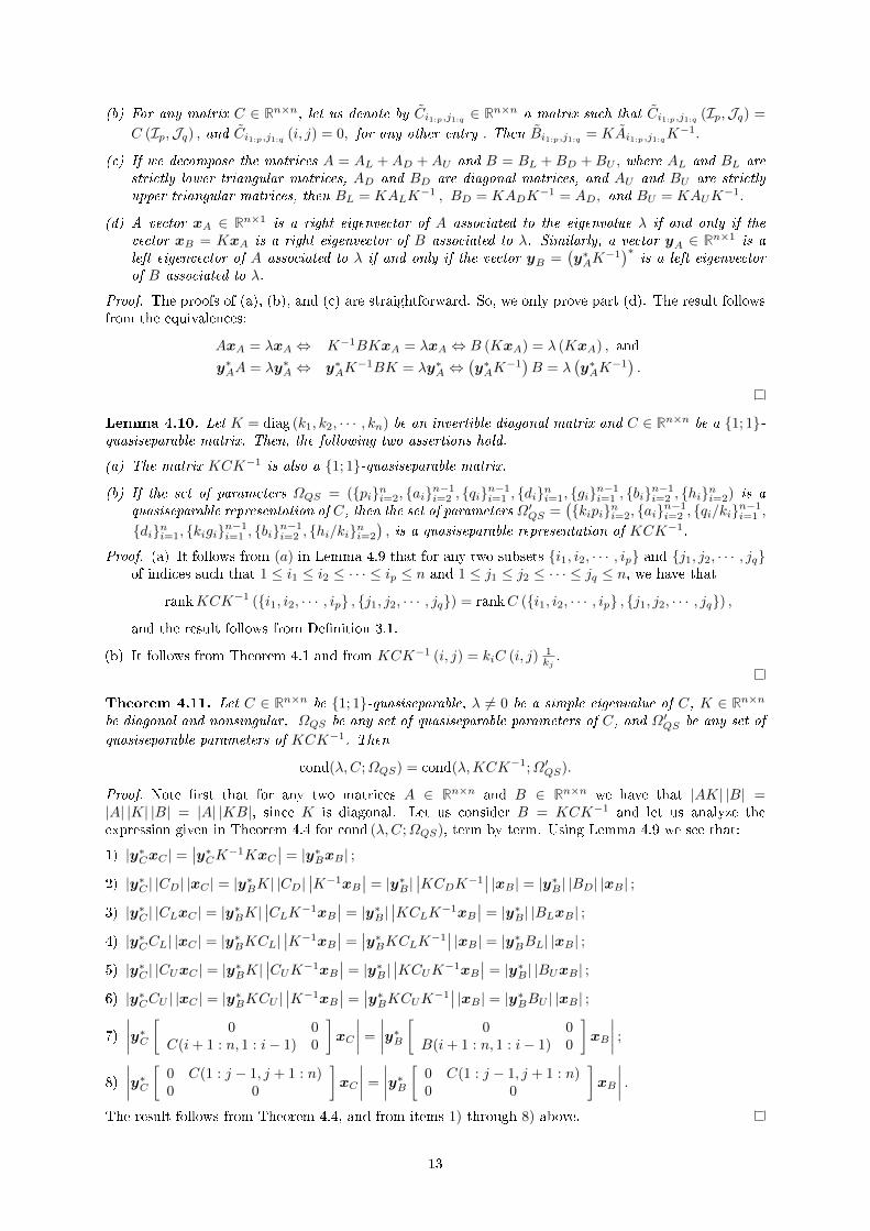
(b) For any matrix C ∈ Rn×n, let us denote by Ci1:p,j1:q ∈ Rn×n a matrix such that Ci1:p,j1:q (Ip,Jq) =

C (Ip,Jq) , and Ci1:p,j1:q (i, j) = 0, for any other entry . Then Bi1:p,j1:q = KAi1:p,j1:qK−1.

(c) If we decompose the matrices A = AL + AD + AU and B = BL + BD + BU , where AL and BL arestrictly lower triangular matrices, AD and BD are diagonal matrices, and AU and BU are strictlyupper triangular matrices, then BL = KALK

−1 , BD = KADK−1 = AD, and BU = KAUK

−1.

(d) A vector xA ∈ Rn×1 is a right eigenvector of A associated to the eigenvalue λ if and only if thevector xB = KxA is a right eigenvector of B associated to λ. Similarly, a vector yA ∈ Rn×1 is aleft eigenvector of A associated to λ if and only if the vector yB =

(y∗AK

−1)∗ is a left eigenvectorof B associated to λ.

Proof. The proofs of (a), (b), and (c) are straightforward. So, we only prove part (d). The result followsfrom the equivalences:

AxA = λxA ⇔ K−1BKxA = λxA ⇔ B (KxA) = λ (KxA) , and

y∗AA = λy∗A ⇔ y∗AK−1BK = λy∗A ⇔

(y∗AK

−1)B = λ(y∗AK

−1) .Lemma 4.10. Let K = diag (k1, k2, · · · , kn) be an invertible diagonal matrix and C ∈ Rn×n be a 1; 1-quasiseparable matrix. Then, the following two assertions hold.

(a) The matrix KCK−1 is also a 1; 1-quasiseparable matrix.

(b) If the set of parameters ΩQS = (pini=2, ain−1i=2 , qi

n−1i=1 , dini=1, gi

n−1i=1 , bi

n−1i=2 , hini=2) is a

quasiseparable representation of C, then the set of parameters Ω′QS =(kipini=2, ai

n−1i=2 , qi/ki

n−1i=1 ,

dini=1, kigin−1i=1 , bi

n−1i=2 , hi/kini=2

), is a quasiseparable representation of KCK−1.

Proof. (a) It follows from (a) in Lemma 4.9 that for any two subsets i1, i2, · · · , ip and j1, j2, · · · , jqof indices such that 1 ≤ i1 ≤ i2 ≤ · · · ≤ ip ≤ n and 1 ≤ j1 ≤ j2 ≤ · · · ≤ jq ≤ n, we have that

rankKCK−1 (i1, i2, · · · , ip , j1, j2, · · · , jq) = rankC (i1, i2, · · · , ip , j1, j2, · · · , jq) ,

and the result follows from Denition 3.1.

(b) It follows from Theorem 4.1 and from KCK−1 (i, j) = kiC (i, j) 1kj.

Theorem 4.11. Let C ∈ Rn×n be 1; 1-quasiseparable, λ 6= 0 be a simple eigenvalue of C, K ∈ Rn×n

be diagonal and nonsingular, ΩQS be any set of quasiseparable parameters of C, and Ω′QS be any set of

quasiseparable parameters of KCK−1. Then

cond(λ,C;ΩQS) = cond(λ,KCK−1;Ω′QS).

Proof. Note rst that for any two matrices A ∈ Rn×n and B ∈ Rn×n we have that |AK| |B| =|A| |K| |B| = |A| |KB|, since K is diagonal. Let us consider B = KCK−1 and let us analyze theexpression given in Theorem 4.4 for cond (λ,C;ΩQS), term by term. Using Lemma 4.9 we see that:

1) |y∗CxC | =∣∣y∗CK−1KxC

∣∣ = |y∗BxB | ;

2) |y∗C | |CD| |xC | = |y∗BK| |CD|∣∣K−1xB∣∣ = |y∗B |

∣∣KCDK−1∣∣ |xB | = |y∗B | |BD| |xB | ;3) |y∗C | |CLxC | = |y∗BK|

∣∣CLK−1xB∣∣ = |y∗B |∣∣KCLK−1xB∣∣ = |y∗B | |BLxB | ;

4) |y∗CCL| |xC | = |y∗BKCL|∣∣K−1xB∣∣ =

∣∣y∗BKCLK−1∣∣ |xB | = |y∗BBL| |xB | ;5) |y∗C | |CUxC | = |y∗BK|

∣∣CUK−1xB∣∣ = |y∗B |∣∣KCUK−1xB∣∣ = |y∗B | |BUxB | ;

6) |y∗CCU | |xC | = |y∗BKCU |∣∣K−1xB∣∣ =

∣∣y∗BKCUK−1∣∣ |xB | = |y∗BBU | |xB | ;7)

∣∣∣∣y∗C [ 0 0C(i+ 1 : n, 1 : i− 1) 0

]xC

∣∣∣∣ =

∣∣∣∣y∗B [ 0 0B(i+ 1 : n, 1 : i− 1) 0

]xB

∣∣∣∣ ;8)

∣∣∣∣y∗C [ 0 C(1 : j − 1, j + 1 : n)0 0

]xC

∣∣∣∣ =

∣∣∣∣y∗B [ 0 C(1 : j − 1, j + 1 : n)0 0

]xB

∣∣∣∣ .The result follows from Theorem 4.4, and from items 1) through 8) above.

13

4.3 Fast computation of the eigenvalue condition number

The main contribution of this section is that, via Proposition 4.12, we will provide an algorithm forcomputing the eigenvalue condition number cond (λ;ΩQS) for any simple eigenvalue of any 1; 1-quasiseparable matrix C of size n × n in O(n) operations. Taking into account that fast algorithmsfor computing all the eigenvalues of a quasiseparable matrix cost O(n2) ops [43], our result allows usto compute the condition numbers of all the eigenvalues of a quasiseparable matrix also in O(n2) ops.

We remark that the diculty of computing cond (λ;ΩQS) fast comes mainly from the terms:

n−1∑i=2

∣∣∣∣y∗ [ 0 0C(i+ 1 : n, 1 : i− 1) 0

]x

∣∣∣∣ and n−1∑j=2

∣∣∣∣y∗ [ 0 C(1 : j − 1, j + 1 : n)0 0

]x

∣∣∣∣ ,that appear in the formula given in Theorem 4.4. Note that the computation of these terms may beavoided, as a consequence of Proposition 4.8, if we estimate cond (λ;ΩQS) via conde (λ;ΩQS).

Proposition 4.12. Let C ∈ Rn×n be a 1; 1-quasiseparable matrix with a simple eigenvalue λ 6= 0 withleft eigenvector y and right eigenvector x, and assume that λ,x,y, and a quasiseparable representationΩQS of C are all known. Then, cond (λ;ΩQS) can be computed in 42n− 66 ops.

Proof. This proof consists of giving an algorithm for calculating cond (λ;ΩQS). We will count the numberof ops needed for calculating the expression of cond (λ;ΩQS), term by term as follows.

(a) The factor |λ| |y∗x| =

∣∣∣∣∣λn∑i=1

yixi

∣∣∣∣∣ requires 2n ops.

(b) Since every product yixi has already been calculated in (a), the term |y∗| |CD| |x| =

n∑i=1

|di| |yixi|,

can be calculated in 2n− 1 ops.

(c) For the term |y∗| |CLx| , we will calculate the products CLx and C(−2)L x simultaneously, where

C(−2)L denotes the matrix that is obtained from CL by setting to zero the entries (CL)i+1,i for

i = 1, 2, . . . , n − 1, and that will be used later for calculating the term in (g). For simplicity, let us

denote the vectors wlx = C(−2)L x and zlx = CLx. Notice that wlx1 = wlx2 = 0 and zlx1 = 0. The

fast method for calculating CLx is given by the following algorithm.

Routine 1 (Computes zlx = CLx and wlx = C(−2)L x taking as inputs the quasiseparable parameters

pini=2, ain−1i=2 , qi

n−1i=1 , and the entries xini=1 of x.)

zlx1 = wlx1 = wlx2 = 0tlx1 = q1 · x1zlx2 = p2 · tlx1

for i = 3 : n

tlx2 = ai−1 · tlx1wlxi = pi · tlx2tlx1 = tlx2 + qi−1 · xi−1zlxi = pi · tlx1

endfor

The fact that Routine 1 indeed computes zlx = CLx and wlx = C(−2)L x can be proved easily by

induction. Observe that Routine 1 uses the temporary variables tlx1 and tlx2, in addition to theentries of the vectors zlx and wlx. We warn the reader that these variables will be used also inAlgorithm 1 for computing cond(λ;ΩQS) and are described in the table right before Algorithm 1.

From Routine 1, we see that the cost of calculating CLx and C(−2)L x is 5n− 8 ops, and taking into

account that (CLx)1 = 0 it is straightforward that the cost of calculating |y∗| |CLx| and |C(−2)L x|

simultaneously is 7n− 11 ops.

(d) For the term |y∗CL| |x| , we can use a similar procedure to that in Routine 1 to compute zly = y∗CLand wly = y∗C

(−2)L by starting with the last components of these two row vectors. As before, this

can be done at the cost of 5n − 8 ops, and then, the cost of calculating |y∗CL| |x| and y∗C(−2)L is

7n− 11 ops.

14

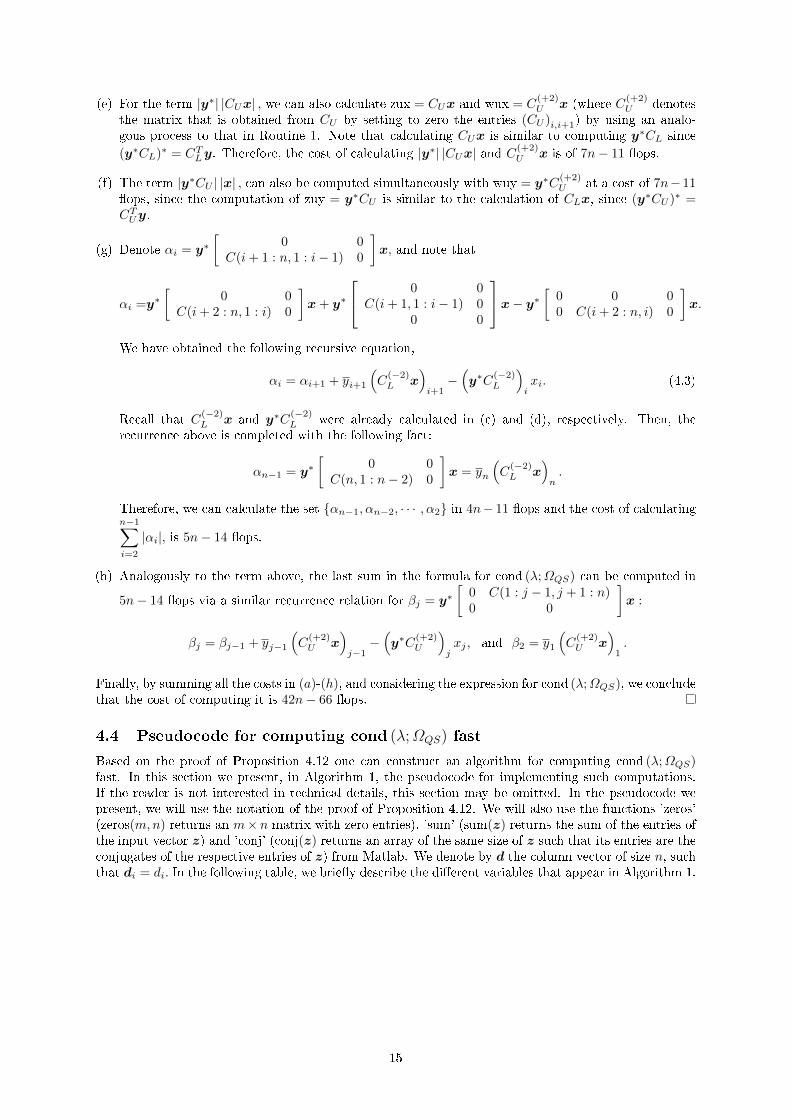
(e) For the term |y∗| |CUx| , we can also calculate zux = CUx and wux = C(+2)U x (where C

(+2)U denotes

the matrix that is obtained from CU by setting to zero the entries (CU )i,i+1) by using an analo-gous process to that in Routine 1. Note that calculating CUx is similar to computing y∗CL since

(y∗CL)∗ = CTLy. Therefore, the cost of calculating |y∗| |CUx| and C(+2)U x is of 7n− 11 ops.

(f) The term |y∗CU | |x| , can also be computed simultaneously with wuy = y∗C(+2)U at a cost of 7n− 11

ops, since the computation of zuy = y∗CU is similar to the calculation of CLx, since (y∗CU )∗ =CTUy.

(g) Denote αi = y∗[

0 0C(i+ 1 : n, 1 : i− 1) 0

]x, and note that

αi =y∗[

0 0C(i+ 2 : n, 1 : i) 0

]x + y∗

0 0C(i+ 1, 1 : i− 1) 0

0 0

x− y∗[

0 0 00 C(i+ 2 : n, i) 0

]x.

We have obtained the following recursive equation,

αi = αi+1 + yi+1

(C

(−2)L x

)i+1−(y∗C

(−2)L

)ixi. (4.3)

Recall that C(−2)L x and y∗C

(−2)L were already calculated in (c) and (d), respectively. Then, the

recurrence above is completed with the following fact:

αn−1 = y∗[

0 0C(n, 1 : n− 2) 0

]x = yn

(C

(−2)L x

)n.

Therefore, we can calculate the set αn−1, αn−2, · · · , α2 in 4n− 11 ops and the cost of calculatingn−1∑i=2

|αi|, is 5n− 14 ops.

(h) Analogously to the term above, the last sum in the formula for cond (λ;ΩQS) can be computed in

5n− 14 ops via a similar recurrence relation for βj = y∗[

0 C(1 : j − 1, j + 1 : n)0 0

]x :

βj = βj−1 + yj−1

(C

(+2)U x

)j−1−(y∗C

(+2)U

)jxj , and β2 = y1

(C

(+2)U x

)1.

Finally, by summing all the costs in (a)-(h), and considering the expression for cond (λ;ΩQS), we concludethat the cost of computing it is 42n− 66 ops.

4.4 Pseudocode for computing cond (λ;ΩQS) fast

Based on the proof of Proposition 4.12 one can construct an algorithm for computing cond (λ;ΩQS)fast. In this section we present, in Algorithm 1, the pseudocode for implementing such computations.If the reader is not interested in technical details, this section may be omitted. In the pseudocode wepresent, we will use the notation of the proof of Proposition 4.12. We will also use the functions 'zeros'(zeros(m,n) returns an m× n matrix with zero entries), 'sum' (sum(z) returns the sum of the entries ofthe input vector z) and 'conj' (conj(z) returns an array of the same size of z such that its entries are theconjugates of the respective entries of z) from Matlab. We denote by d the column vector of size n, suchthat di = di. In the following table, we briey describe the dierent variables that appear in Algorithm 1.

15

Variable Description

zlx zlx = CLx

wlx wlx = C(−2)L x

zly zly = y∗CL

wly wly = y∗C(−2)L

zux zux = CUx

wux wux = C(+2)U x

zuy zuy = y∗CU

wuy wuy = y∗C(+2)U

tlx1 temporary variable introduced for the fast computation of zlx = CLxtly1 temporary variable introduced for the fast computation of zly = y∗CLtux1 temporary variable introduced for the fast computation of zux = CUxtuy1 temporary variable introduced for the fast computation of zuy = y∗CU

tlx2 temporary variable introduced for the fast computation of wlx = C(−2)L x

tly2 temporary variable introduced for the fast computation of wly = y∗C(−2)L

tux2 temporary variable introduced for the fast computation of wux = C(+2)U x

tuy2 temporary variable introduced for the fast computation of wuy = y∗C(+2)U

α vector such that α(i) = αi with αi as in (g) in the proof of Proposition 4.12β vector such that β(i) = βi with βi as in (h) in the proof of Proposition 4.12

Algorithm 1 Fast computation of the eigenvalue condition number cond (λ;ΩQS)

Input: quasiseparable parameters pini=2, ain−1i=2 , qi

n−1i=1 , dini=1, gi

n−1i=1 , bi

n−1i=2 , hini=2, the

eigenvalue λ of C, the respective left and right eigenvectors y and x.Set zlx= zeros (n, 1), wlx= zeros (n, 1), zly= zeros (1, n), wly= zeros (1, n),zux = zeros (n, 1), wux = zeros (n, 1), zuy = zeros (1, n), wuy = zeros (1, n);tlx1 = q1 · x1, zlx2 = p2 · tlx1, tly1 = yn · pn, zlyn−1 = qn−1 · tly1,tux1 = xn · hn, zuxn−1 = gn−1· tux1, tuy1 = g1 · y1, zuy2 = h2 · tuy1.for i=3 to n dotlx2 = ai−1 · tlx1, wlxi = pi · tlx2, tlx1 = tlx2 + qi−1 · xi−1, zlxi = pi · tlx1;tly2 = an−i+1 · tly1, wlyn−i+1 = qn−i+1 · tly2, tly1 = tly2 + pn−i+2 · yn−i+2,zlyn−i+1 = qn−i+1 · tly1;tux2 = bn−i+1 · tux1, wuxn−i+1 = gn−i+1 · tux2, tux1 = tux2 + hn−i+2 · xn−i+2,zuxn−i+1 = gn−i+1 · tux1;tuy2 = bi−1 · tuy1, wuyi = hi · tuy2, tuy1 = tuy2 + gi−1 · yi−1, zuyi = hi · tuy1.

end for

Set α = zeros (1, n), β = zeros (1, n), αn−1 = yn · wlxn, β2 = y1 · wux1.for i=3 to n-1 doαn−i+1 = αn−i+2 + yn−i+2 · wlxn−i+2 − wlyn−i+1 · xn−i+1;βi = βi−1 + yi−1 · wuxi−1 − wuyi · xi;

end for

Set yx = conj(y) . ∗ x;cond (λ;ΩQS) =

( ∣∣d′∣∣ · |yx|+ |y′| · |zlx|+ |zly| · |x|+ |y′| · |zux|+ |zuy| · |x|+sum (|α|) + sum(|β|)

)/(|λ| · |sum(yx)|).

Output: cond (λ;ΩQS).

We remark that the temporary variables tlx1, tlx2, tly1, tly2, tux1, tux2, tuy1, and tuy2 have beenintroduced in order to save operations.

5 Eigenvalue condition numbers for 1; 1-quasiseparable matri-

ces in the Givens-vector representation

This section has, partially, a similar structure to the previous one. We will devote Section 5.1 todescribe the Givens-vector representation [40], while the new results on eigenvalue condition numbersfor this representation are presented in Sections 5.2, 5.3 and 5.4. However, some of the most important

16

properties of these condition numbers will be studied in Section 6.

5.1 The Givens-vector representation for 1; 1-quasiseparable matrices

Another important representation for 1; 1-quasiseparable matrices is the Givens-vector representationintroduced in [40]. This representation was introduced to improve the numerical stability of fast matrixcomputations involving quasiseparable matrices with respect to other representations, but a rigorousproof that this is indeed the case has never been given. The results in this paper are a rst contributionto the solution of this problem. The next theorem shows that this representation is able of representingthe complete class of 1; 1-quasiseparable matrices (see [42, Sections 2.4 and 2.8 ]).

Theorem 5.1. A matrix C ∈ Rn×n is a 1; 1-quasiseparable matrix if and only if it can be parameterizedin terms of the following set of parameters,

• ci, sin−1i=2 , where (ci, si) is a pair of cosine-sine with c2i + s2i = 1 for every i ∈ 2, 3, · · · , n− 1,

• vin−1i=1 , dini=1, ein−1i=1 all of them independent real parameters,

• ri, tin−1i=2 , where (ri, ti) is a pair of cosine-sine with r2i + t2i = 1 for every i ∈ 2, 3, · · · , n− 1,

as follows:

C =

d1 e1r2 e1t2r3 · · · e1t2 . . . tn−2rn−1 e1t2 . . . tn−1c2v1 d2 e2r3 · · · e2t3 . . . tn−2rn−1 e2t3 . . . tn−1

c3s2v1 c3v2 d3 · · · e3t4 . . . tn−2rn−1 e3t4 . . . tn−1...

......

. . ....

...cn−1sn−2 . . . s2v1 cn−1sn−2 . . . s3v2 cn−1sn−2 . . . s4v3 · · · dn−1 en−1sn−1sn−2 . . . s2v1 sn−1sn−2 . . . s3v2 sn−1sn−2 . . . s4v3 · · · vn−1 dn

.

This representation is denoted by ΩGVQS , i.e., ΩGVQS :=

(ci, sin−1i=2 , vi

n−1i=1 , dini=1, ei

n−1i=1 , ri, ti

n−1i=2

).

From Theorems 4.1 and 5.1, it is obvious that the Givens-vector representation is a particular case ofthe quasiseparable representation for 1; 1-quasiseparable matrices by considering the following relationsbetween the parameters in Theorems 4.1 and 5.1, respectively: pi, ain−1i=2 = ci, sin−1i=2 , qi

n−1i=1 =

vin−1i=1 , dini=1 = dini=1, gin−1i=1 = ein−1i=1 , bi, hi

n−1i=2 = ti, rin−1i=2 , and pn = hn = 1. This fact

can be observed better by comparing the expression in Example 4.2 and the expression in the following5× 5 example.

Example 5.2. Let C ∈ R5×5 be a 1; 1-quasiseparable matrix, and let

ΩGVQS :=(ci, sin−1i=2 , vi

n−1i=1 , di

ni=1, ein−1i=1 , ri, ti

n−1i=2

)be a Givens-vector representation of C. Then,

C =

d1 e1r2 e1t2r3 e1t2t3r4 e1t2t3t4

c2v1 d2 e2r3 e2t3r4 e2t3t4c3s2v1 c3v2 d3 e3r4 e3t4

c4s3s2v1 c4s3v2 c4v3 d4 e4s4s3s2v1 s4s3v2 s4v3 v4 d5

.Note that the Givens-vector representation can be made unique if ci and ri are taken to be nonnegative

numbers (if ci = 0, take si = 1 and if ri = 0, take ti = 1) [42, p.76].

5.2 The eigenvalue condition number for 1; 1-quasiseparable matrices in

the Givens-vector representation

Since the Givens-vector representation is a particular case of a quasiseparable representation, one mightthink that it makes no sense to study again eigenvalue condition numbers because we know, from Propo-sition 4.5, that they are independent of the particular choice of ΩQS . However, the subtle point here isthat the Givens-vector representation has correlated parameters since the pairs ci, si are not indepen-dent; the same happens for ri, ti. Since arbitrary componentwise perturbations of ΩGVQS destroy the

17

cosine-sine pairs, and we want to restrict ourselves to perturbations that preserve the cosine-sine pairs,an additional parametrization of these pairs is needed.

Avoiding the use of trigonometric functions, we essentially have two options for this additional pa-rameters:

(a) We can consider ci, si =√

1− s2i , sin−1i=2

and ri, ti =√

1− t2i , tin−1i=2

, but this is not con-

venient because if si is too close to 1, then tiny relative variations of si may produce large relativevariations of ci, since:

sici

∂ci∂si

= − s2ici√

1− s2i= −

(sici

)2

.

This is reected in the following term of the eigenvalue condition number:

siλ

∂λ

∂si=

1

λ (y∗ x)y∗

0 0

−(sici

)2C(i, 1 : i− 1) 0

C(i+ 1 : n, 1 : i− 1) 0

x,

which may be huge if(sici

)2is huge. The same happens for ri.

(b) On the other hand, we can use tangents as parameters in the following way:

ci =1√

1 + l2i, si =

li√1 + l2i

, and ri =1√

1 + u2i, ti =

ui√1 + u2i

, for i = 2, . . . , n− 1.

Observe that when using the tangents as parameters, the value ci = 0 (resp. ri = 0) corresponds toli =∞ (resp. ui =∞). In addition, recall that, since we are interested in calculating relative-relativecomponentwise condition numbers, the parameters that are zero must remain zero. This is consistentwith the fact that ∂ci

∂liand ∂si

∂liboth tend to zero when li →∞. The same happens with ∂ri

∂uiand ∂ti

∂ui

when ui →∞.

Since it is obvious from (b) that tiny relative perturbations of the tangents parameters li and ui producetiny relative perturbations of the cosine-sine parameters ci, si and ri, ti, respectively, it is convenientto use tangents parameters in practical numerical situations. This is related to and inspired by the factthat Givens rotations are computed in practice by using tangents or cotangents. See on this point theclassical reference [26, Algorithm 5.1.3] and the state-of-the-art algorithm in [8].

Denition 5.3. For any Givens-vector representation

ΩGVQS =(ci, sin−1i=2 , vi

n−1i=1 , di

ni=1, ein−1i=1 , ti, ri

n−1i=2

)of a 1; 1-quasiseparable matrix C ∈ Rn×n, we dene the Givens-vector representation via tangents as

ΩGV :=(lin−1i=2 , vi

n−1i=1 , di

ni=1, ein−1i=1 , ui

n−1i=2

), where

ci =1√

1 + l2i, si =

li√1 + l2i

, and ri =1√

1 + u2i, ti =

ui√1 + u2i

, for i = 2, . . . , n− 1.

The next theorem is the main result of this section and it presents an explicit expression for calculatingthe componentwise eigenvalue condition number in the Givens-vector representation via tangents.

Theorem 5.4. Let C ∈ Rn×n be a 1; 1-quasiseparable matrix, let λ 6= 0 be a simple eigenvalue ofC with right eigenvector x and left eigenvector y, and let C = CL + CD + CU , with CL strictly lowertriangular, CD diagonal, and CU strictly upper triangular. Then

cond(λ;ΩGV ) =1

|λ||y∗x|

|y∗||CD||x|+ |y∗CL||x|+ |y∗||CUx|+

n−1∑i=2

∣∣∣∣∣∣y∗ 0 0

−s2i C(i, 1 : i− 1) 0c2i C(i+ 1 : n, 1 : i− 1) 0

x

∣∣∣∣∣∣+

n−1∑j=2

∣∣∣∣y∗ [ 0 −t2jC(1 : j − 1, j) r2jC(1 : j − 1, j + 1 : n)0 0 0

]x

∣∣∣∣.

18

Proof. As in the proof of Theorem 4.4, we will proceed term by term, using (2.5) in Theorem 2.13.Derivatives with respect to the parameters lin−1i=2 : Note rst that

li∂ci∂li

= − l2i(1 + l2i )

3/2= −s2i ci , li

∂si∂li

=li

(1 + l2i )3/2

= c2i si, and, therefore,

liλ

∂λ

∂li=

1

λ(y∗x)

y∗

0 0−s2i C(i, 1 : i− 1) 0

c2i C(i+ 1 : n, 1 : i− 1) 0

x

, i = 2 : n− 1.

Derivatives with respect to the parameters vjn−1j=1 : Note that

vj∂C

∂vj=

[0 · · · 0 0 0 · · · 00 · · · 0 C(j + 1 : n, j) 0 · · · 0

], which implies

vjλ

∂λ

∂vj=

1

λ(y∗x)y∗CL(:, j)xj .

Derivatives with respect to the parameters dini=1:

diλ

∂λ

∂di=

1

λ(y∗x)diyixi.

Derivatives with respect to the parameters ein−1i=1 :

eiλ

∂λ

∂ei=

1

λ(y∗x)yiCU (i, :)x.

Derivatives with respect to the parameters ujn−1j=2 : We rst note that:

uj∂rj∂uj

= −u2j

(1 + u2j )3/2

= −t2jrj and uj∂tj∂uj

=uj

(1 + u2j )3/2

= r2j tj ,

from which we obtain that

ujλ

∂λ

∂uj=

1

λ(y∗x)

(y∗[

0 −t2jC(1 : j − 1, j) r2jC(1 : j − 1, j + 1 : n)0 0 0

]x

).

Again, as in the proof of Theorem 4.4, we consider the sums involving the partial derivatives with respectto each subset of parameters:

• kl =

n−1∑i=2

∣∣∣∣ liλ ∂λ∂li∣∣∣∣ =

1

|λ(y∗x)|

n−1∑i=2

∣∣∣∣∣∣y∗ 0 0

−s2i C(i, 1 : i− 1) 0c2i C(i+ 1 : n, 1 : i− 1) 0

x

∣∣∣∣∣∣;• kv =

n−1∑j=1

∣∣∣∣vjλ ∂λ

∂vj

∣∣∣∣ =1

|λ(y∗x)|

n−1∑j=1

|y∗CL(:, j)xj | =1

|λ(y∗x)||y∗CL| |x|;

• kd =

n∑i=1

∣∣∣∣diλ ∂λ

∂di

∣∣∣∣ =1

|λ(y∗x)|

n∑i=1

|diyixi| =1

|λ(y∗x)||y∗| |CD| |x|;

• ke =

n−1∑i=1

∣∣∣∣eiλ ∂λ

∂ei

∣∣∣∣ =1

|λ(y∗x)|

n−1∑i=1

|yiCU (i, :)x| = 1

|λ(y∗x)||y∗| |CUx|;

• ku =

n−1∑j=2

∣∣∣∣ujλ ∂λ

∂uj

∣∣∣∣ =1

|λ(y∗x)|

n−1∑j=2

∣∣∣∣y∗ [ 0 −t2jC(1 : j − 1, j) r2jC(1 : j − 1, j + 1 : n)0 0 0

]x

∣∣∣∣.From Theorem 2.13 we have cond(λ;ΩGV ) = kl + kv + kd + ke + ku.

19

From the expression in Theorem 5.4 for the relative condition number in the Givens-vector represen-tation for a given 1; 1-quasiseparable matrix C ∈ Rn×n, we see that it does not only depend on thematrix entries, the eigenvalue λ and on the eigenvectors x and y, but it does also depend on the parame-ters ci, si and ri, ti, which are uniquely determined by the entries of C. Therefore, we have obtainedan important dierence with respect to the relative condition number in a quasiseparable representationpresented in Theorem 4.4. Since the Givens-vector representation does not change trivially under diag-onal similarities, because of these cosines-sines parameters, this condition number is not invariant underdiagonal similarities as we can see from Example 5.5.

Example 5.5. Let C ∈ R3×3 be the 1; 1-quasiseparable matrix generated as in Theorem 5.1 bythe set of Givens-vector parameters given by c2, s2 = 2.3768 × 10−1,−9.7134 × 10−1, v1, v2 =9.8355,−2.9770, d1, d2, d3 = 11.437,−5.3162, 9.7257, e1, e2 = 1.7658, 9.7074, t2, r2 =−9.8216 × 10−1, 1.8806 × 10−1, and denote by ΩCGV the respective tangent-Givens-vector represen-

tation. Consider the matrix K = diag(−1,−1, 6), and denote by ΩKCK−1

GV the tangent-Givens-vectorrepresentation of the matrix KCK−1. Then, for the simple eigenvalue λ = 14.120 and the respective left

and right eigenvectors y =[

9.6472× 10−1, 5.5889× 10−2, −2.5728× 10−1]T

and

x =[−4.7887× 10−1, 3.4548× 10−1, 8.0705× 10−1

]Tof C, we have:

cond(λ,C;ΩCGV ) = 1.1706 6= cond(λ,KCK−1;ΩKCK−1

GV ) = 1.2485.

Nevertheless, we will prove in Proposition 6.4 that eigenvalue condition numbers with respect to thetangent-Givens-vector representation can not suer large variations under diagonal similarities.

5.3 Fast computation of the eigenvalue condition number

In this section we prove that cond(λ;ΩGV ) can be computed fast. This fact is stated in Proposition 5.6,which will be proved by providing an algorithm for computing cond(λ;ΩGV ) in O(n) operations.

Proposition 5.6. Let C ∈ Rn×n be a 1; 1-quasiseparable matrix with a simple eigenvalue λ 6= 0 withleft eigenvector y and right eigenvector x, and assume that λ,x,y, and the Givens-vector representationvia tangents ΩGV of C are all known. Then, cond (λ;ΩGV ) can be computed in 60n− 106 ops.

Proof. As we did in the proof of Proposition 4.12, we will nd the cost of calculating each term in theexpression for cond (λ;ΩGV ).

(a) In the rst place, note that the cost of calculating ci = 1√1+l2i

is obviously 4 ops, and the cost of

computing si = li√1+l2i

, is only 1 op because we have already calculated the denominator√

1 + l2i .

Since the same holds for ri and ti, we conclude that the total cost of calculating ci, sin−1i=2 andri, tin−1i=2 is 10n− 20 ops.

(b) The total cost of computing c2i n−1i=2 ,s2i

n−1i=2 ,r2i

n−1i=2 , and t2i

n−1i=2 is 4n− 8 ops.

(c) The factor |λy∗x| =

∣∣∣∣∣λn∑i=1

yixi

∣∣∣∣∣ can be calculated in 2n ops.

(d) Since every product yixi has already been calculated in (c), the term |y∗| |CD| |x| =

n∑i=1

|di| |yixi|,

can be calculated in 2n− 1 ops.

(e) For computing the products y∗CL, CUx (that explicitly appear in the expression for cond (λ;ΩGV ))and CLx, y

∗CU (which will be, respectively, needed in (g) and (h) in this proof) we can proceed asin (d),(e),(c),(f) in the proof of Proposition 4.12, respectively. In these processes, we obtain simulta-

neously y∗C(−2)L , C

(+2)U x, C

(−2)L x, and y∗C

(+2)U (which will also be needed for the fast computation

of the last two sums in cond (λ;ΩGV )). The total cost of these computations is 20n− 32 ops.

(f) The products |y∗CL| |x| and |y∗| |CUx|, can be calculated at a cost of 2n− 3 ops each.

20

(g) Denote αi := y∗

0 0−s2i C(i, 1 : i− 1) 0

c2i C(i+ 1 : n, 1 : i− 1) 0

x, and note that

αi = y∗

0 0−s2i C(i, 1 : i− 1) 0

0 0

x + y∗

0 00 0

c2i C(i+ 1 : n, 1 : i− 1) 0

x

= −s2i yi(CLx)i + c2i

(y∗[

0 0C(i+ 1 : n, 1 : i− 1) 0

]x

).

The expression −s2i yi(CLx)i can be calculated in 2 ops since s2i and CLx have been calculated al-

ready. On the other hand, all the expressions

(y∗[

0 0C(i+ 1 : n, 1 : i− 1) 0

]x

)can be calculated

via a recurrence relation as in (g) in the proof of Proposition 4.12, in 4n − 11 ops. Consequently,

the vector αin−1i=2 can be calculated in 8n−19 ops, and the cost of computing∑n−1i=2 |αi| is 9n−22

ops.

(h) If we denote βj := y∗[

0 −t2j C(1 : j − 1, j) r2j C(1 : j − 1, j + 1 : n)0 0 0

]x, then we can proceed in

an analogous way to (g), and obtain also a cost for computing∑n−1j=2

∣∣∣βj∣∣∣ of 9n− 22 ops.

Finally, by summing all the costs obtained above, and from the expression for cond(λ;ΩGV ) we obtaina total cost of 60n− 106 ops for computing cond(λ;ΩGV ).

5.4 Pseudocode for computing cond (λ;ΩGV ) fast

In this section we present the pseudocode in Algorithm 2 for computing cond (λ;ΩGV ) fast. Again, ifthe reader is not interested in such technical details then this section may be omitted.

Since any set of Givens-vector parameters can also be considered as a set of quasiseparable param-eters, and since from the proof of Proposition 5.6 we know that cond (λ;ΩGV ) can be calculated in avery similar way to cond (λ;ΩQS), we have that Algorithms 1 and 2 are also similar. Therefore we donot describe Algorithm 2 in detail. We will use the standard functions 'zeros', 'sum', 'conj', and 'ones'from MATLAB. The vectors d, zlx, wlx, zly, wly, zux, wux, zuy, wuy, α, β, and the temporary variablestlx1, tly1, tux1, tuy1, tlx2, tly2, tux2, tuy2, are all dened as in Algorithm 1. In the following table, webriey describe the new variables that appear in the pseudocode of Algorithm 2.

Variable Description

α vector such that α(i) = αi with αi as in the proof of Proposition 5.6

β vector such that β(i) = βi with βi as in the proof of Proposition 5.6

21

Algorithm 2 Fast computation of the eigenvalue condition number cond (λ;ΩGV )

Input: Givens-vector parameters lin−1i=2 , vin−1i=1 , dini=1, ei

n−1i=1 , ui

n−1i=2 , the eigenvalue λ of C, the

respective left and right eigenvectors y and x.Set c = [ones(n− 2, 1)./(sqrt(ones(n− 2, 1) + l.2))], s = l. ∗ c, c = [c; 1];r = [ones(n− 2, 1)./(sqrt(ones(n− 2, 1) + u.2))], t = u. ∗ r, r = [r; 1];zlx = zeros (n, 1), wlx= zeros (n, 1), zly= zeros (1, n), wly= zeros (1, n),zux = zeros (n, 1), wux = zeros (n, 1), zuy = zeros (1, n), wuy = zeros (1, n);tlx1 = v1 · x1, zlx2 = c2 · tlx1, tly1 = yn · cn, zlyn−1 = vn−1 · tly1,tux1 = xn · rn, zuxn−1 = en−1· tux1, tuy1 = e1 · y1, zuy2 = r2·tuy1.for i=3 to n dotlx2 = si−1 · tlx1, wlxi = ci · tlx2, tlx1 = tlx2 + vi−1 · xi−1, zlxi = ci · tlx1;tly2 = sn−i+1 · tly1, wlyn−i+1 = vn−i+1 · tly2, tly1 = tly2 + cn−i+2 · yn−i+2,zlyn−i+1 = vn−i+1 · tly1;tux2 = tn−i+1 · tux1, wuxn−i+1 = en−i+1 · tux2, tux1 = tux2 + rn−i+2 · xn−i+2,zuxn−i+1 = en−i+1 · tux1;tuy2 = ti−1 · tuy1, wuyi = ri · tuy2, tuy1 = tuy2 + ei−1 · yi−1, zuyi = ri · tuy1.

end for

Set α = zeros (1, n), β = zeros (1, n), αn−1 = yn · wlxn, β2 = y1 · wux1.α = zeros (1, n), β = zeros (1, n), αn−1 = −s2n−1 · yn−1 · zlxn−1, β2 = −t22 · zuy2 · x2.for i=3 to n-1 doαn−i+1 = αn−i+2 + yn−i+2 · wlxn−i+2 − wlyn−i+1 · xn−i+1,αn−i+1 = −s2n−i+1 · yn−i+1 · zlxn−i+1 + c2n−i+1 · αn−i+1,βi = βi−1 + yi−1 · wuxi−1 − wuyi · xi,βi = −t2i · zuyi · xi + r2i · βi.

end for

Set yx = conj(y). ∗ x;

cond (λ;ΩGV ) =( ∣∣d′∣∣ · |yx|+ |zly| · |x|+ |y′| · |zux|+ sum (|α|) + sum(

∣∣∣β∣∣∣))/(|λ·| |sum(yx)|).Output: cond (λ;ΩGV ).

6 Comparison of cond(λ;ΩQS) and cond(λ;ΩGV )

As we know, the Givens-vector representation is a particular case of the quasiseparable representationwhich imposes additional constraints on the parameters. Since we will only consider perturbationsrespecting such constraints, that is, preserving the cosine-sine relations in the parameters ci, si andri, ti of ΩGVQS , it is natural to expect cond(λ;ΩGV ) not to be larger than cond(λ;ΩQS). In Theorem6.1, we prove that the Givens-vector representation via tangents is a more stable representation thanthe quasiseparable representation for eigenvalue computations for 1; 1-quasiseparable matrices. Thisis the rst time that a rigorous proof is given in such direction.

Theorem 6.1. Let C ∈ Rn×n be a 1; 1-quasiseparable matrix, ΩGV be the tangent-Givens-vectorparameters of C, ΩQS be any set of quasiseparable parameters of C, and λ 6= 0 be a simple eigenvalue ofC. Then,

cond(λ;ΩGV ) ≤ cond(λ;ΩQS).

Proof. We compare for the same matrix C, the expression given for cond(λ;ΩQS) in Theorem 4.4 andthe expression given in Theorem 5.4 for cond(λ;ΩGV ). Starting from the sums in the last two terms ofthe expression for cond(λ;ΩGV ), we have:

S1 =

n−1∑i=2

∣∣∣∣∣∣y∗ 0 0

−s2i C(i, 1 : i− 1) 0c2i C(i+ 1 : n, 1 : i− 1) 0

x

∣∣∣∣∣∣≤

n−1∑i=2

|yiCL(i, :)x|+n−1∑i=2

∣∣∣∣y∗ [ 0 0C(i+ 1 : n, 1 : i− 1) 0

]x

∣∣∣∣= |y∗| |CLx|+

n−1∑i=2

∣∣∣∣y∗ [ 0 0C(i+ 1 : n, 1 : i− 1) 0

]x

∣∣∣∣. (6.1)

22

Analogously, we obtain:

S2 =

n−1∑j=2

∣∣∣∣y∗ [ 0 −t2j C(1 : j − 1, j) r2j C(1 : j − 1, j + 1 : n)0 0 0

]x

∣∣∣∣≤ |y∗CU | |x|+

n−1∑j=2

∣∣∣∣y∗ [ 0 C(1 : j − 1, j + 1 : n)0 0

]x

∣∣∣∣. (6.2)

From (6.1) and (6.2) we have

cond(λ;ΩGV ) ≤ 1

|λ||y∗x|

|y∗||CD||x|+ |y∗||CLx|+ |y∗CL||x|+ |y∗||CUx|+ |y∗CU ||x|

+

n−1∑i=2

∣∣∣∣y∗ [ 0 0C(i+ 1 : n, 1 : i− 1) 0

]x

∣∣∣∣+

n−1∑j=2

∣∣∣∣y∗ [ 0 C(1 : j − 1, j + 1 : n)0 0

]x

∣∣∣∣

= cond(λ;ΩQS).

On the other hand, we are going to show now that the Givens-vector representation via tangents canonly improve, with respect to a general quasiseparable representation, the relative condition number ofa simple eigenvalue of a quasiseparable matrix, up to a factor of 3n. Therefore, both representations canbe considered equivalent from the point of view of the accuracy of the eigenvalue computations that theyallow. This is proved in Theorem 6.3, for which we need the simple Lemma 6.2. It is worth to observethat results in the spirit of Lemma 6.2 can be found in the detailed error analysis of Givens rotationspresented in [4].

Lemma 6.2. Let l 6= 0 be a real number representing a tangent and c the corresponding positive cosine.Then, for any positive value η < 1, a relative perturbation of l by at most η produces a relative perturbationof c of the order of η, i.e.,∣∣∣∣δll

∣∣∣∣ ≤ η =⇒∣∣∣∣δcc∣∣∣∣ ≤ (η +O(η2)

), where c+ δc =

1√1 + (l + δl)2

.

Proof. Consider l′ = l + δl as the perturbed tangent and c′ = c+ δc = 1/√

1 + (l′)2 as the respectiveperturbed cosine . Then, for 1 > η > 0 suciently small we have that if (1− η)|l| ≤ |l′| ≤ (1 + η)|l|, then

c

1 + η=

1

(1 + η)(√

1 + l2)≤ c′ ≤ 1

(1− η)(√

1 + l2)=

c

1− η,

from where we can conclude that |δl| ≤ η|l| ⇒ |δc| ≤ (η +O(η2))|c|.

Theorem 6.3. Let λ 6= 0 be a simple eigenvalue of a 1; 1-quasiseparable matrix C ∈ Rn×n and ΩGVbe the tangent-Givens-vector representation of C. Then for any quasiseparable representation ΩQS of C:

cond(λ;ΩQS)

cond(λ;ΩGV )≤ 3(n− 2).

Proof. Recall that from the Givens-vector representation via tangents ΩGV of C we can obtain theGivens-vector representation ΩGVQS of C as in Denition 5.3, and that ΩGVQS is also a quasiseparablerepresentation of C as we explained after Theorem 5.1. Therefore, in order to use the denition ofthe componentwise relative eigenvalue condition number for representations, i.e., Denition 2.10, let usconsider a quasiseparable perturbation δΩGVQS of the parameters in ΩGVQS such that |δΩGVQS | ≤ η|ΩGVQS |,and the resulting quasiseparable matrix C := C(ΩGVQS + δΩGVQS ). We will refer to η as the level of the

relative perturbation of the parameters in the representation ΩGVQS . We emphasize that the perturbation

δΩGVQS does not respect in general the pairs cosine-sine.

On the other hand, note that C can also be represented by a set

Ω′GV :=(l′in−1i=2 , v

′in−1i=1 , d

′ini=1, e′in−1i=1 , u

′in−1i=2

)23

of tangent-Givens-vector parameters and let us consider the perturbations δ′ΩGV := Ω′GV − ΩGV . Forsimplicity, we will denote C := C(ΩGVQS +δΩGVQS ) = C(Ω′GV ). The strategy of the proof is to nd an upperbound for the level η′ of the respective relative perturbations in the parameters in Ω′GV produced bythe level η of relative perturbation in the quasiseparable parameters in ΩGVQS , i.e., we will nd a function

η′(η) such that |δΩGVQS | ≤ η|ΩGVQS | ⇒ |δ′ΩGV | ≤ η′(η)|ΩGV |. Let us proceed by analyzing each subset ofparameters as follows.

• For the parameters in d′ini=1 it is obvious that δ′di = δdi.

• For the parameters in v′jn−1j=1 note that v′j =

√√√√ n∑i=j+1

(C(i, j))2 from where it is easy to see that if

|δΩGVQS | ≤ η|ΩGVQS |, then√√√√ n∑i=j+1

[(1− η)nC(i, j)]2 ≤ v′j ≤

√√√√ n∑i=j+1

[(1 + η)nC(i, j)]2,

(1− η)n

√√√√ n∑i=j+1

[C(i, j)]2 ≤ v′j ≤ (1 + η)n

√√√√ n∑i=j+1

[C(i, j)]2,

(1− η)nvj ≤ v′j ≤ (1 + η)nvj ,

and, consequently, we have that |δ′vj | ≤ (nη +O(η2))|vj |, for j = 1, . . . , n− 1.

• For studying the level of perturbation in the parameters l′in−1i=2 produced by the level η of per-

turbation in ΩGVQS + δΩGVQS , recall rst that the parameter pn = 1 of ΩGVQS is also perturbed. Next,

taking into account which are the entries of C in the representations ΩGVQS + δΩGVQS and Ω′GVaccording to Theorems 4.1 and 5.1, observe

l′n−1 =s′n−1c′n−1

=C(n, n− 2)

C(n− 1, n− 2)=

(1 + εn−1)sn−1(1 + αn−1)

cn−1(1 + βn−1), and

l′i =s′ic′i

=C(i+ 1, i− 1)

C(i, i− 1)

1

c′i+1

=ci+1(1 + εi)si(1 + αi)

ci(1 + βi)c′i+1

, for i = n− 2, n− 3, . . . , 2,

(6.3)

where |εi| ≤ η, |αi| ≤ η, |βi| ≤ η, for i = n − 1, n − 2, . . . , 2. From Lemma 6.2, we know thatif |δ′li+1| = |l′i+1 − li+1| ≤ κi+1|li+1|, then |δ′ci+1| = |c′i+1 − ci+1| ≤

(κi+1 +O(κ2i+1)

)|ci+1|, or

equivalently c′i+1 = ci+1(1 + θi+1), with |θi+1| ≤ κi+1 + O(κ2i+1). Therefore, the second equationin (6.3) implies

|δ′li| = |l′i − li| ≤ (3η + κi+1 +O(η2 + κ2i+1))|li| for i = n− 2, n− 3, . . . , 2, (6.4)

and the rst equation in (6.3) implies |δ′ln−1| ≤ (3η +O(η2))|ln−1|, i.e., up to rst order in η, wecan take κn−1 = 3η. So, equation (6.4) provides a recurrence relation for κi+1 and we get

|δ′li| ≤ (3(n− i)η +O(η2))|li|.

• For the parameters in e′in−1i=1 , we can proceed in an analogous way to that for the parameters in

v′jn−1j=1 , and we obtain that |δ′ei| ≤ (nη +O(η2))|ei|, for i = 1, . . . , n− 1.

• For the parameters in u′jn−1j=2 , we can also proceed in an analogous way to that for the parameters

in l′in−1i=2 , and we obtain that |δ′uj | ≤ (3(n− j)η +O(η2))|uj |, for j = 2, . . . , n− 1.

Note that for a 1; 1-quasiseparable matrix C := C(ΩGV ) = C(ΩGVQS ), we have proved, so far, that

given any quasiseparable perturbation |δΩGVQS | ≤ η|ΩGVQS |, there exists a perturbation δ′ΩGV of the

tangent-Givens-vector parameters of C, such that C(ΩGVQS + δΩGVQS ) = C(ΩGV + δ′ΩGV ) and |δ′ΩGV | ≤(3(n− 2)η +O(η2))|ΩGV |. Then, from Denition 2.10, we have:

cond(λ;ΩQS) ≤ limη→0

sup

|δλ|η|λ|

: (λ+ δλ) is an eigenvalue of C(ΩGV + δΩGV ),

|δΩGV | ≤ (3(n− 2)η +O(η2))|ΩGV |.

24

By considering the change of variable η′ = (3(n− 2)η +O(η2)), we obtain

cond(λ;ΩQS) ≤ limη′→0

sup

3(n− 2)|δλ|

η′|λ|: (λ+ δλ) is an eigenvalue of C(ΩGV + δΩGV ) ,

|δΩGV | ≤ η′|ΩGV |

= 3(n− 2)cond(λ;ΩGV ).

From Example 5.5 in Section 5.2 we know that the eigenvalue condition number with respect tothe tangent-Givens-vector representation is not invariant under diagonal similarities. However, fromTheorems 6.1, 6.3, and 4.11, it is straightforward to prove that the variations that may be obtained inthe condition number under these similarities are not signicant from a numerical point of view. This isstated, without proof, in the following proposition.

Proposition 6.4. Let λ 6= 0 be a simple eigenvalue of a 1; 1-quasiseparable matrix C ∈ Rn×n, ΩGVbe the tangent-Givens-vector representation of C, K ∈ Rn×n be diagonal and nonsingular and ΩKCK

−1

GV

be the tangent-Givens-vector representation of KCK−1. Then

1

3(n− 2)≤ cond(λ,C;ΩGV )

cond(λ,KCK−1;ΩKCK

−1

GV

) ≤ 3(n− 2).

7 Numerical experiments

In this section, we will discuss briey some numerical experiments that have been performed in orderto conrm some of the results for eigenvalue condition numbers obtained in Sections 4, 5, and 6. Wehave run several random numerical tests in MATLAB for comparing the unstructured componentwisecondition number cond(λ) in Theorem 2.8 and the structured ones cond(λ;ΩQS) and cond(λ;ΩGV ). Wehave started by generating the vectors

l ∈ Rn−2,v ∈ Rn−1,d ∈ Rn, e ∈ Rn−1, and u ∈ Rn−2, (7.1)

containing the randomly generated parameters of the tangent-Givens-vector representation in Denition5.3, by using the command randn from MATLAB. In addition, in some tests we have scaled the pa-rameters in v and e as explained in (7.2). Then, we build the quasiseparable matrix C of size n × ngenerated by these parameters and we obtain its eigenvalues and eigenvectors using the standard com-mand eig from MATLAB. The parameters in ΩQS := ΩGVQS in Denition 5.3 are also computed. Finally,we compute the structured eigenvalue condition numbers cond(λ;ΩQS) and cond(λ;ΩGV ), using our fastAlgorithms 1 and 2 respectively, and the unstructured condition number cond(λ) using direct matrix-vector multiplication with a resulting cost of order 2n2 + O(n) operations (note that cond(λ) can alsobe computed in O(n) operations since |C| is also a quasiseparable matrix), and we compare these threecondition numbers.

When the generated parameters are completely random (i.e., no scaling has been introduced), we havenot observed large dierences between the eigenvalue condition numbers, i.e., cond(λ) ≈ cond(λ;ΩQS) ≈cond(λ;ΩGV ), and all of them are very often moderate.

On the other hand, as announced above, we have also performed tests where some scalings overthe randomly generated parameters of the tangent-Givens-vector representation have been introduced inorder to build an unbalanced quasiseparable matrix. After generating the random vectors as in (7.1), wehave scaled the parameters in v and e by creating the vectors (using MATLAB standard notation):

scv = (10.(k : −(k − 1)/(n− 2) : 1)) and sce = (10.(1 : (k − 1)/(n− 2) : k)) ,

where k is a xed natural number not greater than 10 in our experiments, and considering

v = 102 ∗ scv. ∗ v and e = 102 ∗ sce. ∗ e , (7.2)

which may produce unbalanced rows and columns in the lower and upper triangular parts of the ma-trix generated by these parameters (see Example 5.2). Therefore, we may expect large unstructuredeigenvalue condition numbers. In this way, for dierent values of k and dierent sizes n, we have founddistributions of the tangent-Givens-vector parameters that produce 1; 1-quasiseparable matrices such

25

that the unstructured condition number cond(λ) is much larger than the structured ones, cond(λ;ΩQS)and cond(λ;ΩGV ). In fact, for n = 200 and n = 300, with k = 5 in both cases, we have obtainedparticular matrices such that:

n λmin λmax maxλ

cond(λ)

cond(λ;ΩQS)

maxλ

cond(λ;ΩQS)

cond(λ;ΩGV )

200 555.2761 −2.4628 · 104 + 1.6840 · 105i 4.7847 · 1011 3.3337300 60.5936 −1.3533 · 105 + 2.6060 · 105i 2.4201 · 1010 3.2570

,

where λmin and λmax denote the respective minimum and maximum eigenvalues in absolute value, while

maxλ

cond(λ)

cond(λ;ΩQS)

and max

λ

cond(λ;ΩQS)

cond(λ;ΩGV )

denote the respective maximum values of the quotients,

both taken over the corresponding sets of the eigenvalues of the particular considered matrices for n = 200and n = 300. Furthermore, if we denote by λopt the eigenvalue where the maximum of the quotient

cond(λ)cond(λ;ΩQS)

occurs, we have:

n λopt cond(λopt) cond(λopt;ΩQS)

200 −2.4569 · 103 + 3.7791 · 102i 2.4780 · 1013 51.7901300 −1.0088 · 104 1.8703 · 1011 7.7281

.

It is worth mentioning that, as one would expect, repeating these experiments for values of k greaterthan 5 (which produce matrices with strongly unbalanced lower and upper triangular parts), we obtainedsimilar results to the ones above.

These examples show not only that the structured eigenvalue condition number cond(λ;ΩQS) (and,therefore, cond(λ;ΩGV )) may be much smaller than the unstructured one cond(λ), but also that thereexist 1; 1-quasiseparable matrices having eigenvalues that are very ill conditioned with respect toperturbations of its entries, but that are very well conditioned with respect to perturbations of itsquasiseparable parameters.

In addition, as one would expect from Theorems 6.1 and 6.3, there is not much dierence betweenthe values of cond(λ;ΩQS) and cond(λ;ΩGV ), therefore we have omitted the corresponding column for

the quotientcond(λ;ΩQS)

cond(λ;ΩGV )in the second table above. In fact, in all our tests we have obtained that

cond(λ;ΩQS)

cond(λ;ΩGV )< 15,

which suggests that the bound in Theorem 6.3 may be improved up to a constant.

8 Conclusions

We have provided a general formula for the relative condition number of a simple eigenvalue of any ma-trix that can be represented by a set of parameters with respect to relative componentwise perturbationsof these parameters. This result has been obtained by using dierential calculus techniques and can begeneralized to other conditioning problems. Based on this formula, we have obtained expressions forthe eigenvalue condition numbers of 1; 1-quasiseparable matrices with respect to relative component-wise perturbations of the parameters in the quasiseparable and the Givens-vector representations, andwe have developed fast algorithms with cost O(n) operations for computing these condition numbers.As far as we know, these results are the rst ones available in the literature dealing with structuredperturbations of low-rank structured matrices. Numerical tests comparing the new structured eigen-value condition numbers with the unstructured componentwise condition number have been performedand have revealed that the eigenvalues of quasiseparable matrices may be very well-conditioned underrelative perturbations of the parameters, but very ill-conditioned under general unstructured relativeperturbations of the matrix entries. In contrast, it has been proved theoretically that the opposite can-not happen. Therefore, for 1; 1-quasiseparable matrices, we have established that the structure shouldplay a key role in the accuracy of eigenvalue computations since the sensitivity of their simple eigenval-ues is potentially much smaller to perturbations of the parameters in the covered representations thanto perturbations of the matrix entries. In addition, we have proved that all considered representationsof 1; 1-quasiseparable matrices are equivalent with respect to the eigenvalue sensitivity and that theGivens-vector representation is the one leading to the smallest eigenvalue condition numbers.

26

Future lines of research related to the results in this paper include to develop and analyze structuredeigenvalue condition numbers for other classes of low-rank structured matrices of higher ranks, as wellas to analyze the structured sensitivity of other problems involving low-rank structured matrices. Inparticular, the authors are presently studying structured condition numbers for the solution of linearsystems of equations whose coecient matrices are quasiseparable.

Acknowledgements. The authors sincerely thank two anonymous referees and the Associate Editorhandling this manuscript (Prof. Ilse Ipsen) for their extremely detailed readings of this long and technicalpaper, for correcting many grammatical typos, and for providing constructive and insightful commentsthat have contributed to a signicant improvement of the original manuscript.

References

[1] Asplund, E., Inverses of matrices aij which satisfy aij = 0 for j > i + p, Math. Scand., 7:57-60,1959.

[2] Asplund, S.O., Finite boundary value problems solved by Green's matrix, Math. Scand., 7:49-56,1959.

[3] Aurentz, J.L., Mach, T., Vandebril, R., Watkins, D.S., Fast and backward stable computa-tion of roots of polynomials, SIAM J. Matrix Anal. Appl., 36(3):942-973, 2015.

[4] Barlow, J.L., Ipsen, I.C.F., Scaled Givens rotations for the solution of linear least squaresproblems on systolic arrays, SIAM J. Sci. Stat. Comput., 8(5):716-733, 1987.

[5] Bebendorf, M., Why nite element discretizations can be factored by triangular hierarchical ma-trices, SIAM J. Numer. Anal., 45(4):1472-1494, 2007.

[6] Bella, T., Olshevsky, V., Stewart, M., Nested product decomposition of quasiseparable ma-trices, SIAM J. Matrix Anal. Appl., 34(4):1520-1555, 2013.

[7] Berger, W.J., Saibel, E., On the inversion of continuant matrices, Frankl. Inst.-Eng Appl.Math., 6:249-253, 1953.

[8] Bindel, D., Demmel, J.W., Kahan, W., Marques, O., On computing Givens rotations reliablyand eciently, ACM Trans. Math. Softw., 28(2):206-238, 2002.

[9] Bini, D.A., Gemignani, L., Pan, V.Y., Fast and stable QR eigenvalue algorithms for generalizedcompanion matrices and secular equations, Numer. Math., 100(3):373-408, 2005.

[10] Bini, D.A., Gemignani, L., Tisseur, F., The Ehrlich-Aberth method for the nonsymmetric tridi-agonal eigenvalue problem, SIAM J. Matrix Anal. Appl., 27(1):153-175, 2005.

[11] Bini, D.A., Boito, P., Eidelman, Y., Gemignani, L., Gohberg, I., A fast implicit QR eigen-value algorithm for companion matrices, Linear Algebra Appl., 432:2006-2031, 2010.

[12] Börm, S., Grasedyck, L., Hybrid cross approximation of integral operators, Numer. Math.,101:221-249, 2005.

[13] Börm, S., Grasedyck, L., Hackbusch, W., Introduction to hierarchical matrices with applica-tions, Eng. Anal. Bound. Elemen., 27:405-422, 2003.

[14] Chandrasekaran, S., Gu, M., Xia, J., Zhu, J., A fast QR algorithm for companion matrices,Recent advances in matrix and operator theory, 111-143, Oper. Theory Adv. Appl., 179, Birkhäuser,Basel, 2008.

[15] Delvaux, S., Van Barel, M., A QR-based solver for rank structured matrices, SIAM J. MatrixAnal. Appl., 30(2):464-490, 2008.

[16] Dopico, F.M., Olshevsky, V., Zhlobich, P., Stability of QR-based fast system solvers for asubclass of quasiseparable rank one matrices, Math. Comp., 82:2007-2034, 2013.

[17] Eidelman, Y., Gohberg, I., On a new class of structured matrices, Integr. Equ. Oper. Theory,34(3):293-324, 1999.

27

[18] Eidelman, Y., Gohberg, I., On generators of quasiseparable nite block matrices, Calcolo, 42:187-214, 2005.

[19] Eidelman, Y., Gohberg, I., Haimovici, I., Separable Type Representations of Matrices andFast Algorithms. Volume 1. Basics. Completion Problems. Multiplication and Inversion Algorithms,Operator Theory: Advances and Applications, 234. Birkhäuser/Springer, Basel, 2014

[20] Eidelman, Y., Gohberg, I., Haimovici, I., Separable Type Representations of Matrices andFast Algorithms. Volume 2. Eigenvalue Method, Operator Theory: Advances and Applications, 235.Birkhäuser/Springer, Basel, 2014

[21] Eidelman, Y., Gohberg, I., Olshevsky V., The QR iteration method for Hermitian quasisep-arable matrices of an arbitrary order, Linear Algebra Appl., 404:305-324, 2005.

[22] Ferreira, C., Parlett, B., Dopico, F.M., Sensitivity of eigenvalues of an unsymmetric tridi-agonal matrix, Numer. Math., 122(3):527-555, 2012.

[23] Fiedler, M., Markham T.L., Generalized totally nonnegative matrices, Linear Algebra Appl.,345:9-28, 2002.

[24] Gantmacher, F.R., Krein, M.G., Oscillation Matrices and Kernels and Small Vibrations ofMechanical Systems, AMS Chelsea Publishing, Providence, Rhode Island, 2002 (revised editionfrom the Russian original edition published in 1941).

[25] Geurts, A.J., A contribution to the theory of condition, Numer. Math., 39:85-96, 1982.

[26] Golub, G.H., Van Loan, C.F., Matrix Computations, 3rd ed., The Johns Hopkins UniversityPress, Baltimore, 1996.

[27] Grasedyck, L., Kriemann, R., Le Borne, S., Parallel black box H-LU preconditioning forelliptic boundary value problems, Comput. Vis. Sci., 11:273-291, 2008.

[28] Higham, N.J., Accuracy and Stability of Numerical Algorithms, 2nd edn., Society for Industrialand Applied Mathematics, Philadelphia, 2002.

[29] Higham, D.J., Higham, N.J., Structured backward error and condition of generalized eigenvalueproblems, SIAM J. Matrix Anal. Appl., 20(2):493-512, 1998.

[30] Ipsen, I.C.F., Relative perturbation results for matrix eigenvalues and singular values, Acta Nu-merica, 7:151-201, 1998.

[31] Karow M., Kressner D., Tisseur F, Structured eigenvalue condition numbers, SIAM J. MatrixAnal. Appl., 28(4):1052-1068, 2006.

[32] Li, R.C., Relative perturbation theory. III. More bounds on eigenvalue variations, Linear AlgebraAppl., 266:337-345, 1997.

[33] Martinsson, P.G., Rokhlin V., A fast direct solver for boundary integral equations in two di-mensions, J. Comput. Phys., 205:1-23, 2005.

[34] Martinsson, P.G., Rokhlin, V., Tygert, M., A fast algorithm for the inversion of generalToeplitz matrices, Comput. Math. Appl., 50:741-752, 2005.

[35] Parlett, B.N., Reinsch, C., Balancing a matrix for calculation of eigenvalues and eigenvectors,Numer. Math., 13:292-304, 1969.

[36] Rice, J.R., A theory of condition, SIAM J. Numer. Anal., 3:287-310, 1966.

[37] Roy, S.N., Sarhan A.E., On inverting a class of patterned matrices, Biometrika, 43:227-231, 1956.

[38] Stewart, G.W., Sun, J., Matrix Perturbation Theory, Academic Press, Boston, 1990.

[39] Van Barel, M., Vandebril, R., Van Dooren, P., Frederix, K., Implicit double shift QR-algorithm for companion matrices, Numer. Math., 116:177-212, 2010.

28

[40] Vandebril, R., Van Barel, M., Mastronardi, N., A note on the representation and denitionof semiseparable matrices, Numer. Linear Algebra Appl., 12:839-858, 2005.

[41] Vandebril, R., Van Barel, M., Golub G., Mastronardi, N., A bibliography on semiseparablematrices, Calcolo, 42:249-270, 2005.

[42] Vandebril, R., Van Barel, M., Mastronardi, N., Matrix Computations and SemiseparableMatrices. Volume 1. Linear Systems, The Johns Hopkins University Press, Baltimore, 2008.

[43] Vandebril, R., Van Barel, M., Mastronardi, N., Matrix Computations and SemiseparableMatrices. Volume II. Eigenvalue and singular value methods, The Johns Hopkins University Press,Baltimore, 2008.

[44] Wilkinson, J.H., The Algebraic Eigenvalue Problem, Oxford University Press, New York, 1965.

29