Structure of Finite Nuclei - UMD Physics · Chapter 8 Structure of Finite Nuclei The nuclear shell model, developed by Mayer and Jensen in 1952, is now a very successful and highly

Chapter 8

Structure of Finite Nuclei

The nuclear shell model, developed by Mayer and Jensen in 1952, is now a very successful andhighly developed microscopic theory for the structure of finite nuclei. We will explore its basicaspects and illustrate its predictive power in this chapter.

We have previously seen that a successful description of nuclear matter can be obtained usinga mean single particle potential and a weak residual N -N effective interaction. We will follow asimilar strategy for finite nuclei. Assume that the Schrodinger equation can be written

Hψ(1, 2, . . . A) = Eψ(1, 2, . . . A) (8.1)

with the Hamiltonian given by

H =∑

i

(

Ti + U(i)

)

+∑

i<j

vij . (8.2)

The single particle potential U(i) and the residual two body interaction vij are both phenomenolog-ical, to be adjusted to reproduce the properties of real nuclei. Similar to the case of nuclear matter,we hope that if we find the “best” U(i) then vij will be weak can be treated as a “perturbation”.

8.1 Magic Nuclei, Single Particle States, And Spin-Orbit Interac-

tions

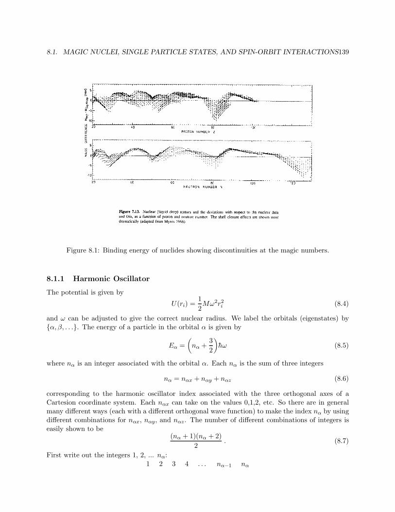
As a first goal, we would hope to reproduce a basic systematic feature of the set of atomic nuclei:the “magic numbers”. Empirically, it is found that there are large deviations from the smoothBethe-Weizacker formula for nuclear binding energies near certain “magic” values of N and Z. Thenuclei with

Z,N = 2, 8, 20, 28, 50, 82, 126have an excess of binding energy. This can be seen in Figure ??.

Such a systematic feature should arise from the properties of the single particle potential U(i),so we first work on the single particle potential. Let the Hamiltonian be

H =∑

i

Ti + U(i) . (8.3)

As a first attempt, let’s explore the shell structure (or magic numbers) that result from a simplesymmetric three dimensional harmonic oscillator potential.

138

8.1. MAGIC NUCLEI, SINGLE PARTICLE STATES, AND SPIN-ORBIT INTERACTIONS139

Figure 8.1: Binding energy of nuclides showing discontinuities at the magic numbers.

8.1.1 Harmonic Oscillator

The potential is given by

U(ri) =1

2Mω2r2i (8.4)

and ω can be adjusted to give the correct nuclear radius. We label the orbitals (eigenstates) byα, β, . . .. The energy of a particle in the orbital α is given by

Eα =

(

nα +3

2

)

hω (8.5)

where nα is an integer associated with the orbital α. Each nα is the sum of three integers

nα = nαx + nαy + nαz (8.6)

corresponding to the harmonic oscillator index associated with the three orthogonal axes of aCartesion coordinate system. Each nαx can take on the values 0,1,2, etc. So there are in generalmany different ways (each with a different orthogonal wave function) to make the index nα by usingdifferent combinations for nαx, nαy, and nαz. The number of different combinations of integers iseasily shown to be

(nα + 1)(nα + 2)

2. (8.7)

First write out the integers 1, 2, ... nα:1 2 3 4 . . . nα−1 nα

140 CHAPTER 8. STRUCTURE OF FINITE NUCLEI

Then place 2 bars somewhere between the integers. There are nα + 1 places for the 1st bar, thennα + 2 places for the second. The number of integers to the left of the left-most bar is nαx, thenumber to the right of the right-most bar is nαz and the number between is nαy. The number ofways to place the bars is

(nα + 1)(nα + 2)

2(8.8)

where we divide by 2 since the bars can be interchanged to give the same result.

Now we fill the orbital α with the maximum number of particles, which is the degeneracy(nα + 1)(nα + 2)/2 times 4 (for spin and isospin). Then we fill all the orbitals nα from 0 up tosome maximum index nmax and count the number of particles:

A = 4 ×nmax∑

nα=0

(nα + 1)(nα + 2)

2=

(nmax + 1)(nmax + 2)(nmax + 3)

6× 4 (8.9)

We also can compute the nuclear radius to evaluate ω:

3

5r20A

2/3 =4

A·

nmax∑

nα=0

〈r2α〉(nα + 1)(nα + 2)

2(8.10)

〈r2α〉 =h

Mω

(

nα +3

2

)

; (virial theorem) (8.11)

(8.12)

so we obtain

hω =42

A1/3MeV. (8.13)

There will be energy “gaps” between shell (orbital) fillings, when we finish filling each orbit. Theseoccur at the values of

N,Z =(n+ 1)(n + 2)(n + 3)

3; n = 0, 1, 2, . . . (8.14)

= 2, 8, 20, 40, 70, 112 (8.15)

Although the first three numbers are a promising start, we find that this potential gives the wrongsequence of magic numbers.

8.1.2 Square Well

Next we try a square well for U(~ri). This more closely approximates the nuclear density, so shouldbe a better choice for the mean potential.

U(r) =

−U0 0 ≤ r ≤ R0 r > R

. (U0 > 0) (8.16)

The interior region Schrodinger equation is

~∇2φα + 2M(U0 − Eα)φα = 0. (8.17)

8.1. MAGIC NUCLEI, SINGLE PARTICLE STATES, AND SPIN-ORBIT INTERACTIONS141

We define k2α ≡ 2M(U0 − Eα) and write the solution in the form φα = Rnl(r)Ylm(Ω) where the

radial equation isd2Rnl

dr2+

2

r

dRnl

dr+

[

k2nl −

l(l + 1)

r2

]

Rnl = 0. (8.18)

The solutions are the spherical Bessel ftns:

Rnl = jl(knlr). (8.19)

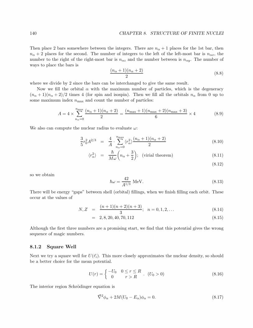
For a deep well, we requirejl(knlR) = 0. (8.20)

One can then find (see e.g., Abramowitz and Stegun, p. 467) the sequence of solutions shown inTable 8.1

knlR 2(2l+1) Sum

π l=0 (0s) 2 24.49 l=1 (0p) 6 85.79 l=2 (0d) 10 18

2π=6.28 l=0 (1s) 2 206.99 l=3 (0f) 14 347.22 l=1 (1p) 6 40

Table 8.1: Magic numbers for the square well potential.

Of course, a finite well will modify this sequence, but not drastically. So a square well cannotgive the correct magic numbers either.

8.1.3 Spin-Orbit Potential

Many potentials have been tried, but none in fact none give the correct sequence of magic numbers.The only successful model uses a spin-orbit potential added to the central potential. A nucleon inthe central region “sees” nucleons on all sides, moving in all directions, and with all spin orienta-tions. Therefore, there would be no spin-orbit force contribution and we expect U(r)=constant,independent of ~σ, ~l. Thus, the spin orbit potential Uso is peaked at the nuclear surface, and isusually something like

Uso(r) =γ

r

dUcent

dr(~l · ~s) = ULS

~l · ~s (8.21)

since dUcent

dr is only large at surface. The origin of this potential is associated with the exchange ofvector mesons (such as the ρ meson) between nucleons.

It is easy to show that the splitting between orbitals with j = l ± 12 is given by a relation

∆ELS = Ej=l+ 1

2

− Ej=l− 1

2

= 〈ULS〉(

l +1

2

)

. (8.22)

∆ELS = 〈ULS〉1

2

[

j(j + 1) − l(l + 1) − 3

4

]

l+ 1

2

−[

j(j + 1) − l(l + 1) − 3

4

]

l− 1

2

(8.23)


=1

2〈ULS〉

[(

l +1

2

)(

l +3

2

)

−(

l − 1

2

)(

l +1

2

)]

(8.24)

= 〈ULS〉(

l +1

2

)

(8.25)

We will see that 〈ULS〉 < 0 is the choice that gives the correct sign of the splitting.Also, the Woods-Saxon potential is commonly used for the central potential:

U(r) =U0

1 + e(r−c)/a0(8.26)

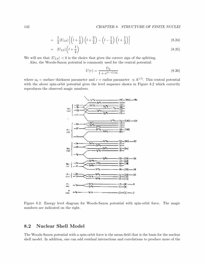
where a0 = surface thickness parameter and c = radius parameter ∝ A1/3. This central potentialwith the above spin-orbit potential gives the level sequence shown in Figure 8.2 which correctlyreproduces the observed magic numbers.

Figure 8.2: Energy level diagram for Woods-Saxon potential with spin-orbit force. The magicnumbers are indicated on the right.

8.2 Nuclear Shell Model

The Woods-Saxon potential with a spin-orbit force is the mean-field that is the basis for the nuclearshell model. In addition, one can add residual interactions and correlations to produce more of the

8.2. NUCLEAR SHELL MODEL 143

details of the structure of nuclei. Here we confine ourselves to the basic features that one can studyusing the mean field potential.

8.2.1 Filled Orbitals

States associated with filled orbitals are the “magic” nuclei where Z or N is one of the magicnumbers. Many nuclei with Z or N close to magic numbers can be treated with the filled orbitalplus a few particles “holes”. Consider an orbital with quantum numbers nlj which is filled with2j + 1 particles, m = −j,m = j + 1, . . . m = j − 1,m = j. Clearly we have

M =∑

i

mi = 0.

The wave function can be written as a Slater determinant

ψnlj =

∣∣∣∣

φm=−j(1) φm=−j+1(1) . . .φ−j(2) φ−j+1(2) . . .

∣∣∣∣ (8.27)

For each term we haveJz

∏

i

φmi(i) = 0. (8.28)

In addition, the antisymmetry of ψnlj implies that, for each i, J±(i)ψnlj = 0 so that J±ψnlj = 0.Thus we have

J2 =1

2(J+J− + J−J+) + J2

Z = 0 (8.29)

and so J = 0 and M = 0 for a filled orbital. The parity is given by [(−)l]2j+1. Since 2j + 1 mustbe an even integer, we obtain π = +. Therefore, a filled orbital has Jπ = 0+

8.2.2 Single particle in orbital

Now consider the case of a single particle in an orbital nlj.

Jzφnljm(1) = mφnljm(1) (8.30)

J2φnljm = j(j + 1)φnljm (8.31)

So the total z component of angular momentum is

J totz = Jz|filled + Jz = Jz (8.32)

andJ tot 2 = J2|filled + 2 ~Jfilled · ~J + J2 = J2 (8.33)

So we have J = j and parity π = (−)l.

8.2.3 Hole in orbital

We designate with Φ−1 the state with all levels filled except nljm. Then

JzΦ−1 = −mΦ−1 (8.34)

J2Φ−1 = j(j + 1)Φ−1 (8.35)

since we can couple Φ−1 and φjm to J = 0.


8.2.4 2 Particles in Orbital

Now consider two particles in the states nljm and nljm′. We can write a Slater determinant

Φ(j2,mm′) =1√2

∣∣∣∣

φ1(j,m) φ1(j,m′)

φ2(j,m) φ2(j,m′)

∣∣∣∣ (8.36)

and note the property Φ(j2,mm′) = −Φ(j2,m′,m). We can use these to form a state of goodangular momentum

Φ(j2, JM) =∑

m,m′

〈jmjm′|JM〉Φ(j2,mm′) . (8.37)

Now use the symmetry of the Clebsch-Gordon coefficients:

Φ(j2, JM) = (−)2j−J∑

〈jm′jm|JM〉Φ(j2,mm′) (8.38)

= (−)2j−J+1∑

〈jmjm′|JM〉Φ(j2,m′m) . (8.39)

The last line follows from the antisymmetry of the Φ(j2,mm′) and implies that (−)2j−J+1 = +1 or(2j + 1) − J = even. Since 2j + 1 is an even integer, we must have only even values of J ≤ 2j − 1.

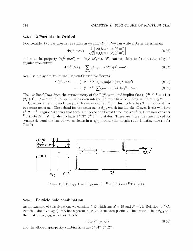
Consider an example of two particles in an orbital, 18O. This nucleus has T = 1 since it hastwo extra neutrons. The orbital for the neutrons is d5/2 which implies the allowed levels will have4+, 2+, 0+. Figure 8.4 shows that these are indeed the lowest three levels of 18O. If we now consider18F (note N = Z), it also includes 1+, 3+, 5+ T = 0 states. These are those that are allowed forsymmetric combinations of two nucleons in a d5/2 orbital (the isospin state is antisymmetric forT = 0).

Figure 8.3: Energy level diagrams for 18O (left) and 18F (right).

8.2.5 Particle-hole combination

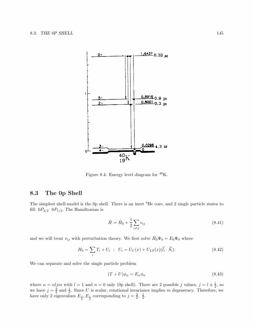
As an example of this situation, we consider 40K which has Z = 19 and N = 21. Relative to 40Ca(which is doubly magic), 40K has a proton hole and a neutron particle. The proton hole is d3/2 andthe neutron is f7/2, which we denote

(πd3/2)−1(νf7/2) (8.40)

and the allowed spin-parity combinations are 5−, 4−, 3−, 2−.

8.3. THE 0P SHELL 145

Figure 8.4: Energy level diagram for 40K.

8.3 The 0p Shell

The simplest shell-model is the 0p shell. There is an inert 4He core, and 2 single particle states tofill: 0P3/2 0P1/2. The Hamiltonian is

H = H0 +1

2

∑

i6=j

vij (8.41)

and we will treat vij with perturbation theory. We first solve H0Ψ0 = E0Ψ0 where

H0 =∑

i

Ti + Ui ; Ui = UC(x) + ULS(x)(~li · ~Si). (8.42)

We can separate and solve the single particle problem

(T + U)φα = Eαφα (8.43)

where α = nljm with l = 1 and n = 0 only (0p shell). There are 2 possible j values, j = l ± 12 , so

we have j = 32 and 1

2 . Since U is scalar, rotational invariance implies m degeneracy. Therefore, wehave only 2 eigenvalues E 3

2

, E 1

2

corresponding to j = 32 ,

12 .


α1 α2 T J

32

32 T=1 2,0

32

32 T=0 3,1

12

12 T=1 0

12

12 T=0 1

32

12 T=1 2,1

32

12 T=0 2,1

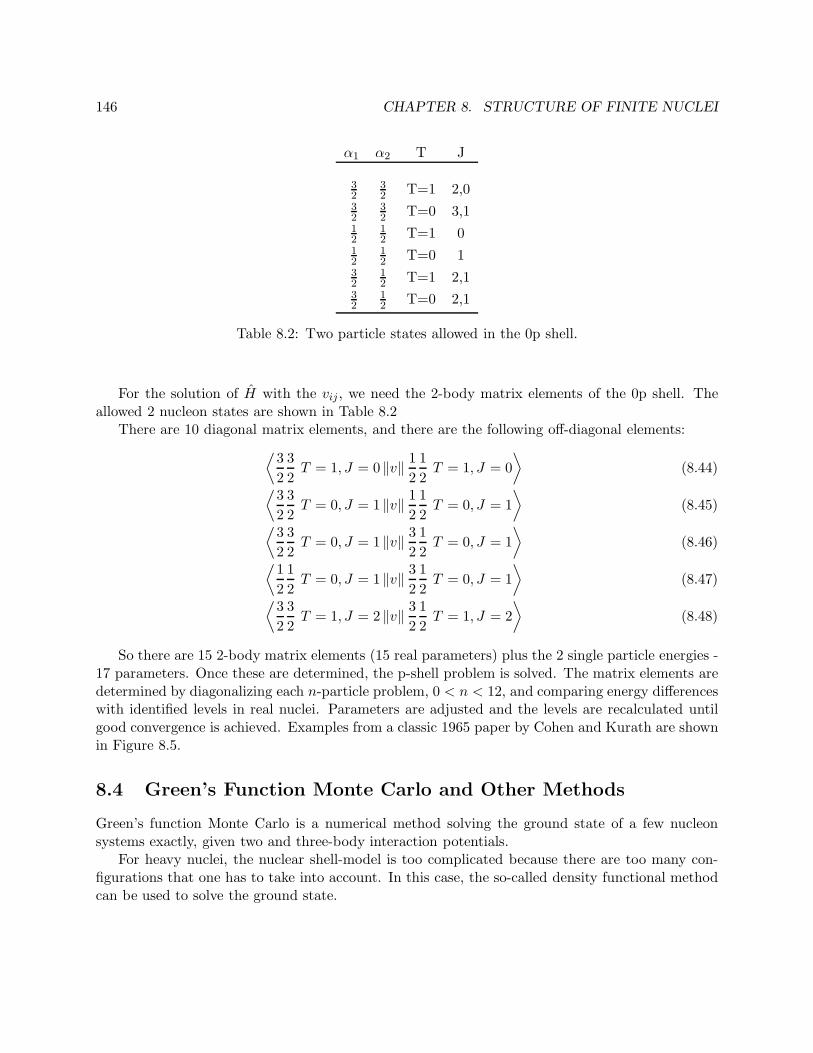
Table 8.2: Two particle states allowed in the 0p shell.

For the solution of H with the vij , we need the 2-body matrix elements of the 0p shell. Theallowed 2 nucleon states are shown in Table 8.2

There are 10 diagonal matrix elements, and there are the following off-diagonal elements:

⟨3

2

3

2T = 1, J = 0 ‖v‖ 1

2

1

2T = 1, J = 0

⟩

(8.44)

⟨3

2

3

2T = 0, J = 1 ‖v‖ 1

2

1

2T = 0, J = 1

⟩

(8.45)⟨

3

2

3

2T = 0, J = 1 ‖v‖ 3

2

1

2T = 0, J = 1

⟩

(8.46)

⟨1

2

1

2T = 0, J = 1 ‖v‖ 3

2

1

2T = 0, J = 1

⟩

(8.47)⟨

3

2

3

2T = 1, J = 2 ‖v‖ 3

2

1

2T = 1, J = 2

⟩

(8.48)

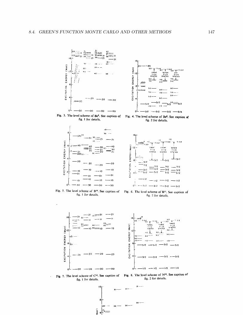
So there are 15 2-body matrix elements (15 real parameters) plus the 2 single particle energies -17 parameters. Once these are determined, the p-shell problem is solved. The matrix elements aredetermined by diagonalizing each n-particle problem, 0 < n < 12, and comparing energy differenceswith identified levels in real nuclei. Parameters are adjusted and the levels are recalculated untilgood convergence is achieved. Examples from a classic 1965 paper by Cohen and Kurath are shownin Figure 8.5.

8.4 Green’s Function Monte Carlo and Other Methods

Green’s function Monte Carlo is a numerical method solving the ground state of a few nucleonsystems exactly, given two and three-body interaction potentials.

For heavy nuclei, the nuclear shell-model is too complicated because there are too many con-figurations that one has to take into account. In this case, the so-called density functional methodcan be used to solve the ground state.

8.4. GREEN’S FUNCTION MONTE CARLO AND OTHER METHODS 147

Chapter 9

Big-Bang Nucleosynthesis

After the universe cooled to a temperature of a few MeV, the energy density was still dominated bythe large number of relativistic particles, all in thermal equilibrium: photons, electrons, positrons,neutrinos and antineutrinos. In addition there were the nucleons (neutrons and protons) thatrepresent the baryonic matter that we observe today.

The number density of the gas of relativistic particles is given by (see Eq. 2.2):

n = gnζ(3)

π2T 3 . (9.1)

The quantity gn is related to the degeneracy of each species present, and is given by

gn = 2 + (2)(2)

(3

4

)

+ (2)

(3

4

)

Nν (9.2)

where the first term is for photons (2 helicity states), the second term is for e+/e− (2 helicitystates for each), and the last term is for neutrinos/antineutrinos (Nν is the number of light flavorspresent). In the standard model we expect Nν = 3. The factor of 3/4 is the proper weighting forfermions relative to bosons (see Chapter 2).

9.1 Neutron/proton Ratio

The subsequent stages of nucleosynthesis in the early universe are governed by the relative numberof neutrons and protons present (heavier nuclei without neutrons do not exist!). So our first goal isto understand and establish the neutron to proton ratio that results from the era of the Big Bang.

The total number density of nucleons is due to the process that created the excess of baryonsat earlier times, and can only be inferred from observations of the present-day universe. However,the relative number of neutrons and protons is governed by the competing processes

νe + n ↔ p+ e− (9.3)

νe + p ↔ n+ e+ . (9.4)

Since the nucleons are in thermal equilibrium with the leptons, the relative number of neutronsand protons is given by the ratio of Boltzmann factors (see Eq. 2.40)

nn

np=e−

MnT

e−Mp

T

= e−Q

T (9.5)

148

9.1. NEUTRON/PROTON RATIO 149

where Q = Mn−Mp = 1.293 MeV. The processes (9.3, 9.4) are, at early times, rapid relative to theexpansion rate of the universe. But as the universe cools, these processes become slower and theratio of neutrons to protons freezes out. This occurs when the rate for neutron-proton conversionΓn↔p falls below the expansion rate (given by Eq. 2.14), or

Γn↔p <R

R. (9.6)

The conversion rate Γn↔p is governed by the weak interaction cross sections for the processesin (9.3) and (9.4). The cross section for

νe + p→ n+ e+ (9.7)

can be computed using the methods used in Chapter 3 to compute the rate of neutron beta decay. Atlow energies (< 10 MeV), the same matrix elements as for the beta decay n→ p e ν are responsiblefor the transition. To compute the cross section, we take the transition probability per unit timeand divide by the incident flux (which for the relativistic neutrinos is c the speed of light):

dσ =dω

c=

2π

hc|Hfi|2

dN

dEf. (9.8)

The density of final states is given by

dN

dEf=

d3pe

(2πh)3=

p2e

(2πh)3dpe

dEf· dΩ . (9.9)

We then integrate over the final β angle:

σ =

∫dσ

dΩdΩ = 4π ·

[2π

hc|Hfi|2

]

· p2e

(2πh)3dpe

dEf. (9.10)

We neglect the recoil energy of the final nucleus: dEf∼= dEe and we use pe dpe = Ee dEe to obtain

the result

σ =1

πh4 |Hfi|2 · peEe (9.11)

where

|Hfi|2 = G2F

[

M2F + g2

AM2GT

]

(9.12)

= G2F

[

1 + 3g2A

]

(9.13)

as in Eq. ??. The final positron energy Ee is related to the incident νe energy by

Eν = Q+Ee + Tn (9.14)

≃ Q+Ee (9.15)

since at these energies the neutron recoil kinetic energy Tn ∼ 1 keV is negligible relative to the otherquantities. Recalling that gA ≃ 1.26 and neglecting the electron mass we arrive at the approximateexpression:

σ ≃ GF2(Eν −Q)2 (9.16)

150 CHAPTER 9. BIG-BANG NUCLEOSYNTHESIS

where we now use units with h = 1. In the early universe the neutrinos are in thermal equilibriumat temperature T :

σ ∼ G2F (T −Q)2 . (9.17)

The rate Γn↔p can be writtenΓn↔p = nν〈σv〉 (9.18)

where nν is the neutrino number density and v(= c) the neutrino velocity. The number density ofneutrinos is just

nν =3

4

ζ(3)

π2T 3 (9.19)

and we findΓn↔p ≃ G2

FT3(T −Q)2/2 . (9.20)

The actual value depends upon the neutron lifetime, which is required as input to obtain andaccurate value for the quantity M2

F + g2AM

2GT .

Now using Eq. 2.14 and Eq. 2.4 we find

R

R≃√

g∗GNT2 (9.21)

(here GN is Newton’s constant) and where we recall (see Chapter 2) that

g∗ = 2 + (2)(2)

(7

8

)

+ (2)

(7

8

)

. (9.22)

We can now solve for the freeze-out temperature where

Γn↔p ∼ R

R(9.23)

to obtain

Tf (Tf −Q)2 ∼√g∗GN

G2F

. (9.24)

Evaluating this expression yields an estimate for the freeze-out temperature of

Tf ∼ 1 MeV . (9.25)

We can now use this value in Eq. 9.5 to obtain

nn

np≃ 1

6. (9.26)

(The actual value is sensitive to some details like Nν , which makes the subsequent nucleosynthesisand final abundances of light elements also sensitive to this interesting quantity.) Finally, after thefreeze-out some of the neutrons decay before the nuclear reactions associated with nucleosynthesis(that traps them in stable nuclei) occurs, and the actual value is given by

nn

np≃ 1

7. (9.27)

9.2. PRODUCTION OF DEUTERIUM AND HELIUM 151

9.2 Production of Deuterium and Helium

The first step in the chain of nuclear reactions in the early universe is the capture of protons andneutrons to form deuterium

n+ p→ d+ γ(2.225 MeV). (9.28)

When the temperature is low enough that the high photon density is reduced sufficiently that thedeuterons are stable (T ∼ 0.1 MeV), further reactions can begin to take place. The next step is

p+ d→ 3He + γ(7 MeV) (9.29)

followed byp+ 3He → 4He + γ(20 MeV). (9.30)

The end product of this chain of reactions, 4He, is very stable and so very little of it is processedfurther. In fact, essentially all of the neutrons end up in 4He. The cross sections for proton captureon deuterium and 3He are quite high and so the rates are fast compared to the expansion rate. Inaddition, the high photon energies required for the inverse reactions prohibit the photodisintegrationreactions so, effectively, at these low temperatures only single captures are important. In the end,only a small number of d and 3He remain when all the neutrons are captured and essentially allof them are in 4He. Thus, the fractional abundance of 4He is given simply by the neutron-protonratio Eq. 9.27. One obtains the result for the mass fraction of 4He, designated Yp,

Yp ≡ 4nHe

nH + 4nHe(9.31)

=2(

nn

np

)

1 + nn

np

(9.32)

≃ 2/7

8/7= 0.25 . (9.33)

The actual value depends mildly upon η, the baryon to photon ratio, but this is a actually areasonably good estimate. The best observational data to date indicate that the primordial valueof Yp = 0.249 ± 0.009, in excellent agreement with the calculations. This is a very impressive androbust prediction of Big Bang Nucleosynthesis, and is a major cornerstone in modern cosmology.

The residual amounts of d and 3He are rather small ∼ 10−5 as they are efficiently converted to4He. The actual amount is quite sensitive to the expansion rate, the nuclear reaction rates, and thetemperature, but can be reliably computed during the phase until the endpoint of 4He production.The predicted values for these abundances are very sensitive to the η, the baryon to photon ratioand are shown in Fig. 9.1.

9.3 Relic Neutrinos

The era of Big Bang Nucleosynthesis marks the point in the history of the universe where the weakinteractions between neutrinos and baryons terminate, and the neutrinos are thereafter decoupled.At this point, we have a relativistic Fermi gas of neutrinos, three flavors, with a total density givenby

nν = 33

4

ζ(3)

π2T 3 . (9.34)


Figure 9.1: The relative abundances of d, 3He, 4He and 7Li are shown as a function of the baryonto photon ratio η10 = η × 1010. The measured values from astronomical observations are shown ashorizontal bands (1σ and 2σ). The curves are the predictions from BBN nucleosynthesis (widthis the estimated uncertainty) and the vertical band at η10 ≃ 6 is the value extracted from fits ofmeasurements of the cosmic microwave background.

9.3. RELIC NEUTRINOS 153

The subsequent evolution of this sea of neutrinos is simply governed by the expansion of theuniverse. Shortly after the decoupling of the neutrinos (at T ∼ 1 MeV) the photons are reheatedby the annihilation of positrons. This reheating is isentropic, so the entropy given by Eq. 2.7 isconserved. Before reheating, we have

s =2

3g0∗

(

T 0)3

(9.35)

with g0∗ = 2 + 7/2 corresponding to the photons and e± (the neutrinos are decoupled). Afterward,

we have

s =2

3g∗T

3 (9.36)

with g∗ = 2. Therefore we find that the ratio of final to initial temperatures are

(T

T 0

)

=

(

g0∗

g∗

)1/3

(9.37)

Thus the density of photons increases as

nγ

n0γ

=

(T

T 0

)3

(9.38)

=

(

g0∗

g∗

)

(9.39)

=

(

1 +7

4

)

=11

4. (9.40)

Following this reheating, the photons and neutrinos both evolve based on the expansion of theuniverse. The ratios of temperatures Tν/Tγ and the number densities nν/nγ remain constant. Atpresent, measurements of the cosmic microwave background yield the values Tγ = 2.725 K andnγ = 410.4cm−3. Thus, if the neutrinos have light enough masses (i.e., mµ ≪ Tν) we would predictfor the neutrinos today:

Tν =

(4

11

)1/3

Tγ = 1.95 K (9.41)

and a total number density

nν = 33

4(

4

11nγ) = 336 cm−3 (9.42)

where we have accounted for antineutrinos as well as neutrinos with only one helicity state each.

The neutrino masses are known to be light, less than about 1 eV, but are not zero. Throughmeasurements of neutrino oscillations, the mass differences

∆m223 ≃ 3 × 10−3 eV2 (9.43)

∆m212 ≃ 7 × 10−5 eV2 (9.44)

have been determined. Given the current neutrino temperature Tν = 1.7× 10−4 eV, at least two of

the neutrino states are non-relativistic (i.e.,√

∆m223 >

√

∆m212 > Tν). With at least one neutrino


mass (the heaviest = mh) mh >√

∆m223 ≃ 0.05 eV we obtain a lower limit on the energy density

of the neutrinos

Ων >nν

3mh (9.45)

> 6 eV/cm−3 (9.46)

> 10−3Ω0 (9.47)

where Ω0 is the total energy density of the universe. The present experimental upper limit on themass of the νe is 3 eV. With the small mass differences implied by Eq. 9.43 and Eq. 9.44 it ispossible that all three neutrinos have a mass of ∼ 3 eV, which implies the upper bound

Ων < 0.2Ω0 . (9.48)

This is the largest possible value based on direct experimental data on neutrino masses. Anindirect limit on the neutrino density has been obtained by recent analyses of the cosmic microwavebackground measurements using the WMAP satellite data:

Ων < 0.015Ω0 . (9.49)

Thus it appears that the neutrino contribution to the energy of the universe is somewhat less thanthe baryonic matter (Ωb = 0.044Ω0), but is likely at least comparable to the visible luminous matterin stars (Ωlum = 0.005Ω0).

Chapter 10

The Power and Evolution of Stars

It is now well-established that fusion reactions provide the energy to make stars like the sun shine.The sun is a typical “main-sequence” star that is about 5 billion years old. In this chapter we willstudy the nuclear processes that power the energy output of the sun as a prototypical main-sequencestar.

The sun is essentially a ball of 1.2× 1057 hydrogen atoms, compressed by their mutual gravita-tional attraction, with a total mass of M⊙ = 1.98×1030 kg. The solar radius is R⊙ = 6.96×108 m,implying an average density of 1.4 g/cm3, but it is not constant and the density at the center of thesun is about 150 g/cm3. The energy output (solar luminosity), in the form of thermal radiation, isL⊙ = 3.8 × 1026 Watts = 2.4 × 1039 MeV/s.

The gravitational compression heats the solar interior, but it is easy to demonstrate that thisgravitational energy is insufficient to power the solar luminosity. Thus, we require another sourceof energy to make the sun shine so brightly for so long. The basic process that starts this processis a weak interaction, the fusion of two protons into a deuteron:

p+ p→ d+ e+ + ν . (10.1)

The fact that this is a weak interaction makes the cross section very small at the energies providedby the interior solar temperature (∼ 1.5 × 107 K). The energy produced in this reaction is

2Mp −Md −me = 0.420 MeV (10.2)

and is primarily shared between the positron and neutrino in the final state. The neutrino escapesfrom the sun, but the positron’s energy (including its rest mass) becomes part of the thermal energyproduced by nuclear reactions in the solar interior.

The subsequent nuclear reactions involving deuterium and 3He actually provide more energy,but this reaction governs the rate of “hydrogen burning” in the sun. At the central temperatureand density of the sun, this p−p fusion reaction has a mean time constant of 1.4×1010 years. Thisis essentially the reason that the sun can shine steadily for billions of years.

10.1 Nuclear Fusion

The fusion of charged particles at low energy is the dominant nuclear process occurring in starslike the sun. Here we consider the fusion of two nuclei with atomic numbers Z1 and Z2, separated

155

156 CHAPTER 10. THE POWER AND EVOLUTION OF STARS

by a distance r. For r > R1, the strong interaction potential between the nuclei can be neglectedand the potential is just the coulomb potential VC(r) = Z1Z2e

2/r. For light nuclei (A < 16) theradius R1 ∼ 1−2 fm, and the coulomb barrier is EC = VC(R1) > 1 MeV. This is large compared tothe typical kinetic energy kT ∼ 1 keV. Thus the cross section for fusion is suppressed by the hugepotential barrier that must be penetrated for the nuclear potential to take effect (i.e., where thenuclei overlap). In addition, one generally finds the condition for quasi-classical behavior is easilyfulfilled:

η ≡ Z1Z2e2

hv≫ 1 (10.3)

where v is the relative velocity of the nuclei. In this case, one can use the WKB approximation tocompute the penetration through the barrier:

Pl ≃ exp

[

−2√

2µ

h

∫ R2

R1

[Vl(r) −E]1/2 dr

]

(10.4)

in which µ is the reduced mass, R2 is the classical turning point [Vl(R2) = E] and we have defined

Vl(r) ≡ VC(r) +l(l + 1)h2

2µr2. (10.5)

At very low energies, one can usually neglect l > 0 and keep only the s− wave, and the exponentin Eq. 10.4 can be evaluated in the limit E << EC as

2√

2µ

h

∫ R2

R1

[Vl(r) − E]1/2 dr =2πZ1Z2e

2

hv≡ 2πη . (10.6)

The s−wave cross section for the nuclear fusion reaction can generally be written as

σ ≃ π

k2P0 (10.7)

where hk is the momentum in the center of mass frame. Thus we expect the low energy crosssection to depend on energy as

σ =S(E)

Ee−2πη (10.8)

where S(E) is expected to be a slowly varying function of E (for the case where there are noresonances at low energies). S is known as the astrophysical S−factor, and is the quantity that isusually calculated and compared to experimental data through the inverse of Eq. 10.8.

For the p − p fusion reaction Eq. 10.1 the S−factor is given by S11(0) = 4 × 10−22 keV-barns,which at the central solar temperature implies a tiny average cross section of

〈σpp〉 ≃ 4 × 10−51 cm2 . (10.9)

The fact that Eq. 10.1 is a weak process, along with the coulomb penetration factor, combine toproduce this very small cross section that implies the sun will shine for billions of years.

Following the process 10.1, the deuteron that is formed can readily fuse with another protonto form 3He:

p+ d→ 3He + γ . (10.10)

10.1. NUCLEAR FUSION 157

The S−factor for this process, S12 is much larger than S11

S12 ≃ 2.5 × 10−4 keV − b . (10.11)

Thus the deuterons produced in Eq. 10.1 only last a few seconds after they are created. Thereforea significant concentration of deuterium does not build up, but instead there is a growth in theconcentration of 3He.

In the final step of the p− p chain of reaction, two 3He will fuse to form 4He:

3He + 3He → 4He + 2p . (10.12)

This reaction has a healthy S−factor, given by

S33 ≃ 5.3 MeV − b (10.13)

but the higher coulomb barrier penetration and lower concentration of 3He moderates the rate ofthis reaction. The result is that 3He reacts on time scale of order a million years in the center ofthe sun.

While other small branches contribute, this is the major reaction chain that converts protonsinto the tightly bound 4He. The positrons produced in the initial p-p fusion reactions annihilatewith electrons into photons (e+ + e− → 2γ) so actually the complete sequence converts 4 protonsand 2 electrons into 4He, 2 ν’s and electromagnetic energy (that eventually leads to the thermalenergy associated with “sunshine”):

2e− + 4p → 4He + 2ν . (10.14)

The total energy released in this chain of reactions is

Erelease = 4MH −M(4He) − 2〈Eν〉 (10.15)

= 26.7MeV (10.16)

where MH and M(4He) are the atomic masses (including electrons) of Hydrogen and 4He.The energy released, Erelease can be combined with the solar luminosity L⊙ = 3.83 × 1033

ergs/sec to calculate the expected production rate of p-p neutrinos to be 1.8 × 1038 sec−1 whichyields a flux at the earth of

φpp = 6.4 × 1010 cm−2s−1 . (10.17)

This is an extremely important result, and follows only from assuming the p-p chain reactions,energy conservation, and the solar luminosity. More detailed calculations that take into accountother small contributions to the solar luminosity predict

φpp = 6.00 × 1010 cm−2s−1 . (10.18)

A star like the sun will burn hydrogen for billions of years, converting the protons into 4He.There is no stable nucleus with A = 5, so there is no opportunity for the 4He to capture a proton andthus the star will steadily increase its concentration of 4He. A dense core of 4He forms, contractingand increasing in temperature driven by the increased gravitational binding. Outside this core ishydrogen which is heated by the 4He core. Hydrogen burning continues at the surface of the 4Hecore, heating the hydrogen envelope so that it greatly expands. A star like the sun will expand itsradius to about 200 times the current solar radius when it reaches this “red giant” phase. When thehydrogen fuel is exhausted, a star like the sun becomes a ball of gradually cooling 4He. Actually,some of the 4He is processed in helium burning, a process that is more important for heavier starswith M > 3M⊙.


10.2 Helium burning

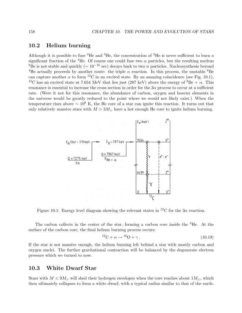
Although it is possible to fuse 4He and 3He, the concentration of 3He is never sufficient to burn asignificant fraction of the 4He. Of course one could fuse two α particles, but the resulting nucleus8Be is not stable and quickly (∼ 10−16 sec) decays back to two α particles. Nucleosynthesis beyond4He actually proceeds by another route: the triple α reaction. In this process, the unstable 8Becan capture another α to form 12C in an excited state. By an amazing coincidence (see Fig. 10.1),12C has an excited state at 7.654 MeV that lies just (287 keV) above the energy of 8Be + α. Thisresonance is essential to increase the cross section in order for the 3α process to occur at a sufficientrate. (Were it not for this resonance, the abundance of carbon, oxygen and heavier elements inthe universe would be greatly reduced to the point where we would not likely exist.) When thetemperature rises above ∼ 108 K, the He core of a star can ignite this reaction. It turns out thatonly relatively massive stars with M > 3M⊙ have a hot enough He core to ignite helium burning.

Figure 10.1: Energy level diagram showing the relevant states in 12C for the 3α reaction.

The carbon collects in the center of the star, forming a carbon core inside the 4He. At thesurface of the carbon core, the final helium burning process occurs:

12C + α→ 16O + γ . (10.19)

If the star is not massive enough, the helium burning left behind a star with mostly carbon andoxygen nuclei. The further gravitational contraction will be balanced by the degenerate electronpressure which we turned to now.

10.3 White Dwarf Star

Stars with M < 9M⊙ will shed their hydrogen envelopes when the core reaches about 1M⊙, whichthen ultimately collapses to form a white dwarf, with a typical radius similar to that of the earth:

10.3. WHITE DWARF STAR 159

6000 km. The white dwarf is a star that is stabilized against further collapse by the degeneracypressure of the Fermi gas of electrons. Further thermonuclear reactions are not significant andnucleosynthesis is essentially terminated.

To understand the role of the degenerate electron pressure, we begin by considering a mature(one that is approaching the limit of its available thermonuclear fuel) star composed of atomseach with mass number A. Let there be a total of n nucleons so the number of atoms is n

A . Wedefine the proton fraction x ≡ Z

A so that the total number of electrons is ne = xn (the star iselectrically neutral). After exhausting its thermonuclear fuel the gravitational force exceeds thethermal pressure associated with thermonuclear reactions, and the radius contracts to the pointwhere the density is very high and atoms lose identity. Then the e− form a Fermi gas and thedensity is high enough that the pressure of the Fermi gas (Pauli principle) is the main supportagainst further collapse. This is a “white dwarf” star.

Assuming the temperature is not so high that the non-relativistic approximation is valid for theelectron gas. The degenerate e− gas has the properties:

ne =Ω

3π2k3

f (10.20)

〈T 〉 =3

5

h2k2f

2me=

3h2

10me

(

3π2ne

Ω

)2/3

(10.21)

Ω =4π

3r3, ne = xn (10.22)

so the total kinetic energy is

〈T 〉 =3h2

10mer2

(9πxn

4

)2/3

(10.23)

The total energy of the star is the sum of the total e− kinetic energy and the gravitationalpotential energy. For a uniform sphere, the gravitational potential is

−3

5GM2

r(10.24)

so we have

E(r) =3h2xn

10mer2

(9πxn

4

)2/3

− 3

5

Gn2M2p

r. (10.25)

(The assumption of a uniform sphere is clearly a rather crude approximation, but the results fora correct treatment are quantitatively very similar.) To find the equilibrium radius, we set thederivative of the energy with respect to the radius to zero

dE(r)

dr

∣∣∣∣req

= 0 (10.26)

which yields the result

req =h2x

GnM2pme

(9πxn

4

)2/3

. (10.27)


For M = M⊙ =1 solar mass= nMp we find n = 1.2 × 1057. Now we assume equal numbers ofprotons and neutrons so that x ∼= 1

2 and use

G = 1.32 × 10−52 cm/GeV (10.28)

h = 1.973 × 10−14 GeV − cm (10.29)

Mp = 0.938 GeV (10.30)

me = 5.11 × 10−4 GeV . (10.31)

The radius of the star is

req = 7.1 × 108 cm (≪ 7 × 1010 cm = R⊙) (10.32)

≈ rearth! (10.33)

The volume and density are then

Ω = 1.5 × 1027 cm3

n/Ω = 1030/cm3 . (10.34)

This is much greater than an inverse atomic volume (1024 cm3), so that the atoms are totallyoverlapping and the electrons are not confined to individual atoms. [The average distance betweenatomic nuclei is about 103 fm = 10−2 A, much smaller than the size of an atom, but much largerthan the nuclear size.] The mass density is

ρ = 1.3 × 106 g/cm3 (10.35)

= 1.3 tons/cm3 (10.36)

≪ ρNM ∼ 1014 g/cm3 (10.37)

where ρNM is the mass density of normal nuclear matter. The average electron kinetic energy is〈T 〉 = 0.12 MeV so we are still in the zero temperature limit but since 〈T 〉 is not insignificantcompared to me we are close to needing to consider the electrons as a relativistic Fermi gas. Thus,for masses beyond 1 M⊙ we need relativistic e−.

For ultra-relativistic electrons the Fermi energy and mean total energy are given by the expres-sions (neglecting now the electron mass)

Ef = h

(

3π2ne

Ω

)1/3

(10.38)

〈E〉 =3

4Ef (10.39)

and we then find

E(r) =3hxn

4r

(9πxn

4

)1/3

− 3

5Gn2M2

p

r(10.40)

≡ αn4/3 − βn2

r. (10.41)

10.4. TYPE IA SUPERNOVA 161

Therefore, if we increase n the numerator eventually becomes negative. Then E(r) decreases(becomes more negative) as the radius r decreases and the star will collapse! Thus, there is acritical number ncrit corresponding to E(r) = 0.

n2/3crit =

5hx

4GM2p

(9πx

4

)1/3

(10.42)

ncrit =

(9πx

4

)1/2

·(

5hx

4GM2p

)3/2

(10.43)

=

(9π

4

)1/2

·(

5h

4GM2p

)3/2

x2 (10.44)

=3(125π)1/2

16·(

h

GM2p

)3/2

x2 (10.45)

This is known as the “Chandrasekhar limit”, and numerically(

h

GM2p

)3/2

= 2.2 × 1057 (10.46)

and so the critical number is ncrit = 2.06 × 1057 corresponding to a total mass

ncritMp = 1.7 M⊙ . (10.47)

The actual value, obtained by numerical solution to the equations that establish equilibrium as afunction of radius and including the rest mass of electron, is 1.4M⊙.

10.4 Type Ia Supernova

Type Ia Supernova explosion is one of the spectacular optical events in the Universe. For this reason,Type Ia supernova has been regarded as a standard candle in measuring cosmological distances.

Type Ia supernova is believed to start from a binary system consisting of a white dwarf and anaccompanying main sequence star. In the white dwarf, the helium has burned almost completelyand resulting a core of carbon and oxygen below Chandrasekar limit. However, the white dwarfsteadily accrete matter from its companion and eventually its mass exceeds the limit. Once thishappens, the star will undergo gravitational collapse and release huge amount of gravitationalenergy in the form of heat which leads to nuclear reactions producing heavier elements such asiron, nickel and cobalt by burning carbon and oxygen. These energy produces a huge explosionwhich result in type Ia supernova, and the entire star is almost entirely destroyed in the process.

In the spectrum of light from type Ia supernova, there is no hydrogen line, because the hydrogenhas been burned before the star collapse happens.

10.5 Fusion in Advanced Massive Stars

Heavier stars with M > 9M⊙ can generate higher internal pressures and temperatures that aresufficient to ignite more advanced stages of nuclear burning and continue the process of nucle-osynthesis. For these stars, the hydrogen burning phase is relatively short, only about 10 million


years, before beginning helium and then carbon burning. Once the carbon burning phase begins,the star has only a few thousand years left to complete the chain of rapid nucleosythesis reactionsthat produce heavier elements up to iron. As shown in a previous chapter, the binding energy pernucleon of stable nuclei increases with nuclear mass number A until A = 56, with 56Fe being themost stable nucleus. Beyond 56Fe it is not possible to form heavier nuclei by the fusion process.

Carbon burning proceeds when the temperature reaches ∼ 5 × 108 K and the central densityexceeds 105 g/cm3. The main reaction is

12C + 12C → 24Mg∗ → 20Ne + α . (10.48)

In addition, there are other reaction products and many reactions that involve capturing protons,alphas, neutrons, and beta decays also occur. Nuclei up to A = 35 are produced in significantquantities as a result of these reactions. But Ne and O are the most abundant products of carbonburning.

At higher temperatures (109 K ∼ 100 keV ) and densities (106g/cm3, the neon burning phasebegins. Photodisintegration of Ne produces α particles via γ + 20Ne → 16O + α and these α’s canin turn be captured on 20Ne:

20Ne + α→ 24Mg + γ . (10.49)

Neon burning is followed by oxygen burning, predominantly

16O + 16O → 32S∗ → 28Si + α (10.50)

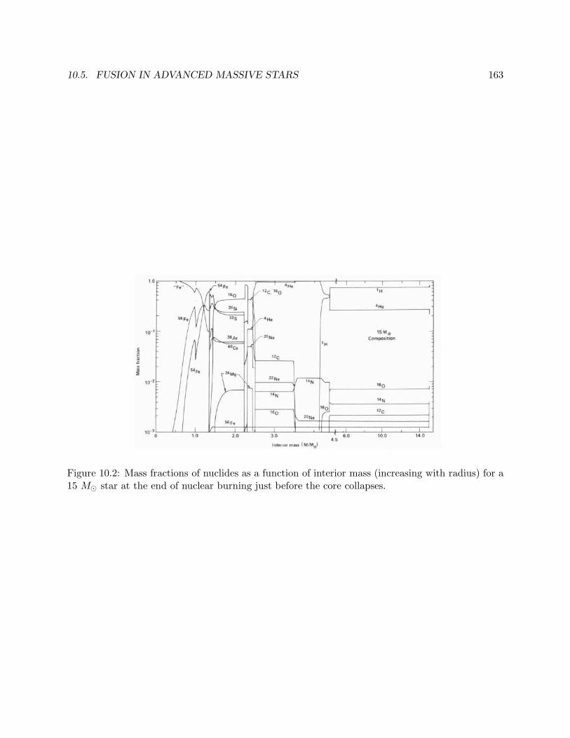
which provides the fuel for silicon burning. Silicon burning involves a complex network of α, p,n, and γ induced reactions that generate nuclei all the way up to 56Ni. The end result of thisprocess is the collection of the most stable nucleus, 56Fe, at the center of the star. The otherburning processes continue in shells outside the Fe core. A calculation of the relative fractions ofnuclides present as a function of interior mass is shown in Fig. 10.2. It can be seen that the star hasan onion-like structure, with different well-defined regions corresponding to the different nuclearburning processes.

If the mass of a star is heavy, the iron core grows until it reaches about 1.4 M⊙, where thedegeneracy pressure of the electrons becomes insufficient to prevent further shrinking. The core willcollapse, and the result is a type II supernova explosion. It is generally thought that the supernovaexplosion is the source of nuclear processes that produce all the elements heavier than iron. Wewill come to this topic later on.

10.5. FUSION IN ADVANCED MASSIVE STARS 163

Figure 10.2: Mass fractions of nuclides as a function of interior mass (increasing with radius) for a15 M⊙ star at the end of nuclear burning just before the core collapses.

Chapter 11

Neutrinos and Neutrino Cosmology

The neutrino was originally invented in 1930 by Pauli to salvage conservation of energy and angularmomentum in nuclear beta decay. At the time it was known that in the beta decay 6He → 6Li+ e−

there were two problems:

• the measured spectrum of electron kinetic energy was a continuous distribution from zero tothe maximum value expected from the difference in masses of 6He and 6Li,

• the spin of 6He is Ji = 0 and the final 6Li has spin Jf = 1, implying the electron should haveintegral angular momentum which is not possible for a fermion.

Thus Pauli had the idea to invent a new neutral fermion emitted with the electron, later known asthe neutrino, that was not detected in the experiments. This would enable restoration of conser-vation of energy and angular momentum.

Due to its lack of electric charge and the weakness of its interactions, the neutrino went unde-tected for many decades. The neutrino was finally observed in experiments in the 1950’s by Reinesand Cowan. These experiments actually were able to detect the antineutrinos emitted by nuclearreactors via the inverse beta decay process νe + p→ e+ + n.

In the latter half of the 20th century, many experiments were performed with muon-type neu-trinos (νµ) produced in accelerator experiments through the decay of pions π+ → µ+ + νµ. Theseνµ (and also νµ) were observed to only produce µ− (or µ+) in their interactions with matter. Thusthey were quite distinct from the νe and νe produced in nuclear beta decays. In addition, thediscovery of the heavier τ lepton introduced another flavor of neutrino, ντ , which was eventuallyobserved as well.

In 1968, Ray Davis and collaborators reported the first observation of neutrinos from the sun.Their experiment involved the use of 100,000 gallons of perchlorethylene (cleaning solution) locateddeep underground (to avoid cosmic rays) in a mine in South Dakota. The chlorine in the detectorcould be transformed into argon through the inverse beta process νe + 37Cl → 37Ar + e−, and theargon atoms could be extracted from the liquid and detected through their decay (37Ar decays withhalf-life t1/2 = 35 days). Although Davis and collaborators reported the observation of a signalindicating the presence of solar neutrinos, the measured rate was more than a factor of 2 less thanthe predicted rate. Throughout the remainder of the 20th century, additional measurements ofsolar neutrinos of various energies all indicated a deficit of flux compared to the expected rates.The issue was finally resolved during the period 1998-2003 when it was established that neutrinos

164

11.1. NUCLEAR BETA DECAY 165

have finite mass and that the flavor eigenstates are not the mass eigenstates. This enables theprocess known as neutrino oscillations, where the flavor states oscillate as the neutrino propagatesthrough space.

The absolute scale of neutrino mass and the basic nature of the neutrino (whether it is its ownantiparticle, i.e., Majorana type, or not i.e, Dirac type fermion) are still to be determined. Nucleiand their properties have been, and continue to be, an essential aspect of the study of neutrinos.

11.1 Nuclear Beta Decay

The process of nuclear beta decay is important both as a means of transforming nuclei into oneanother (in the laboratory and in the stars) and as a crucial means of testing the fundamentalinteraction responsible for it occurrence: the weak interaction. There are three basic processes (allrelated): 1.) electron (β− decay, 2.) positron (β+) decay, and 3.) atomic electron capture. Wefirst consider the definitions of these processes and the energetics associated with each of them.

Electron (β−) decay

This process involves the transformation of a nucleus (Z,N) into (Z+1, N−1) through the emissionof an electron (“β- particle”) and an anti-neutrino (electron-type) νe:

(Z,N) → (Z + 1, N − 1) + e− + νe . (11.1)

The energy released in the process is shared between the e− and νe is known as the “Q value”≡ Q.(A small amount of kinetic energy goes into the recoiling (Z+1, N−1) nucleus, but we will generallyneglect it.)

The simplest example of nuclear beta decay is the decay of the free neutron:

n→ p+ e− + νe . (11.2)

The energy released isQ = Mn −Mp −me −mν . (11.3)

We will see later that we know the neutrino is massless or very light so we may take mν ≃0, andthus

Q = Mn −Mp −me = (939.57 − 938.28 − 0.51)MeV (11.4)

= 0.78MeV. (11.5)

Since the energy is shared between the e− and νe, the maximum kinetic energy of the e− is Q = 0.78MeV.

More generally, for (Z,N) → (Z + 1, N − 1) + e− + νe we define M(Z,N) ≡ atomic mass(including Z electrons) and then

Qβ− = M(Z,N) −M(Z + 1, N − 1) . (11.6)

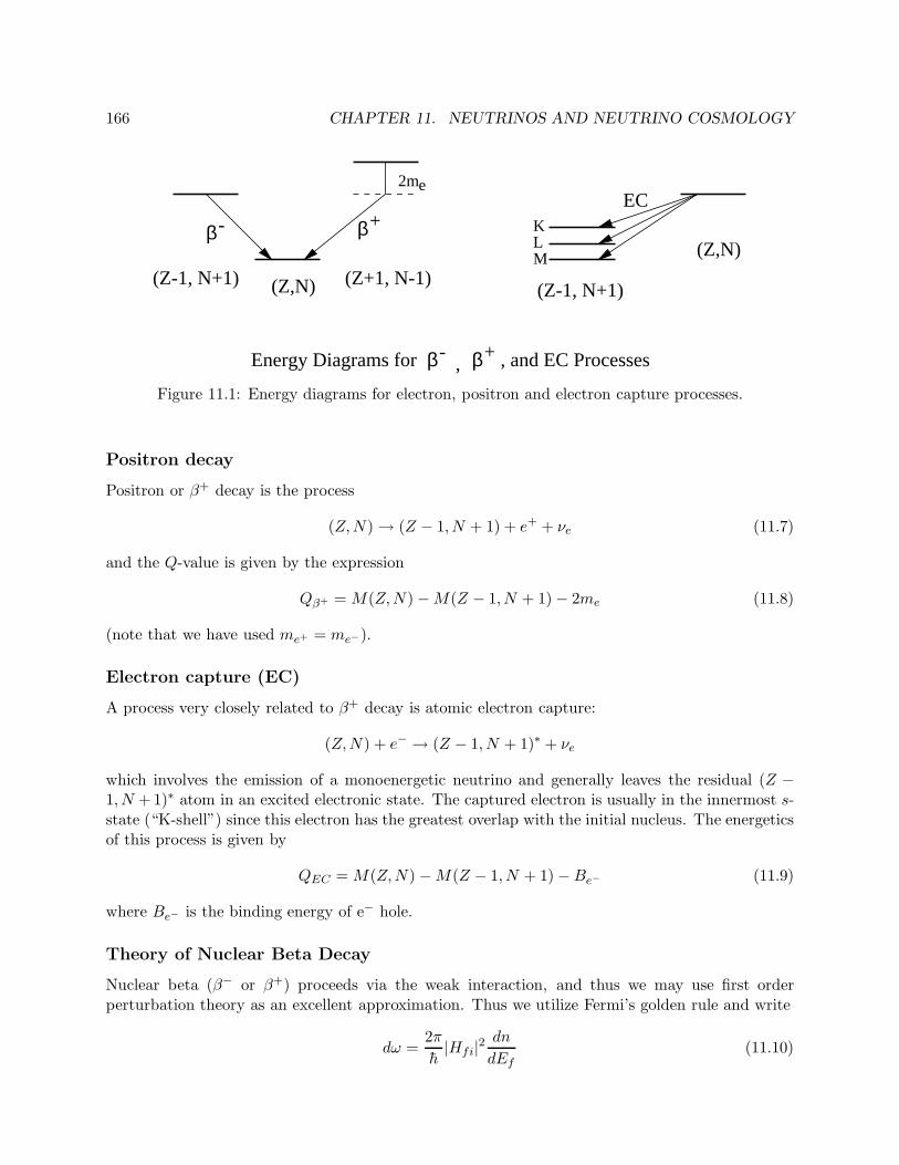
166 CHAPTER 11. NEUTRINOS AND NEUTRINO COSMOLOGY

+-β

-β β+Energy Diagrams for , , and EC Processes

βM

(Z,N)(Z-1, N+1) (Z+1, N-1)(Z-1, N+1)

(Z,N)

EC2me

KL

Figure 11.1: Energy diagrams for electron, positron and electron capture processes.

Positron decay

Positron or β+ decay is the process

(Z,N) → (Z − 1, N + 1) + e+ + νe (11.7)

and the Q-value is given by the expression

Qβ+ = M(Z,N) −M(Z − 1, N + 1) − 2me (11.8)

(note that we have used me+ = me−).

Electron capture (EC)

A process very closely related to β+ decay is atomic electron capture:

(Z,N) + e− → (Z − 1, N + 1)∗ + νe

which involves the emission of a monoenergetic neutrino and generally leaves the residual (Z −1, N + 1)∗ atom in an excited electronic state. The captured electron is usually in the innermost s-state (“K-shell”) since this electron has the greatest overlap with the initial nucleus. The energeticsof this process is given by

QEC = M(Z,N) −M(Z − 1, N + 1) −Be− (11.9)

where Be− is the binding energy of e− hole.

Theory of Nuclear Beta Decay

Nuclear beta (β− or β+) proceeds via the weak interaction, and thus we may use first orderperturbation theory as an excellent approximation. Thus we utilize Fermi’s golden rule and write

dω =2π

h|Hfi|2

dn

dEf(11.10)


where the density of final states may be written

dn

dEf=

d3pe

(2πh)3· d3pν

(2πh)3· δ(E0 − Ee − Eν) (11.11)

where E0 ≡ Q+me = maximum total β energy Ee.We also will assume the long wavelength limit, since generally the lepton momenta pe and pν

are both less than 10 MeV so that the wavelength of the lepton is

λ =2πh

p>∼ 100 fm (11.12)

which is much greater than the nuclear radius. Therefore, Hfi will be independent of pe and pν

but may depend on the angle

cos θeν =~pe · ~pν

pepν. (11.13)

Since we won’t detect the e− direction, nor the ν (direction or energy) we will integrate over thee−, ν angles (note that pν = Eν for mν = 0):

dω =2π

h

∫1

(2π2h3)2|Mfi|2p2

edpep2νdpνδ(E0 − Ee − Eν) (11.14)

=1

2π3h7 |Mfi|2(E0 − Ee)2p2

edpe . (11.15)

Allowing for the Coulomb effect on e− will modify the density of final states, and this has the effectthat we must multiply our result by F (Z,Ee) ≡ “Fermi Function”. In the absence of the Coulombinteraction on the final e−, F (Z = 0, Ee) = 1. Finally, we use that pedpe = EedEe to obtain

dω =1

2π3h7 |Mfi|2F (Z, Ee−)(E0 − E)2peEedEe (11.16)

Beta energy spectrum

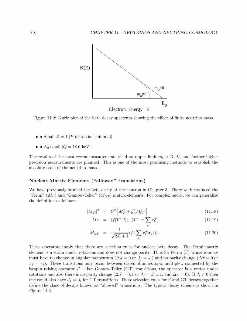
The spectrum of beta energies is then given by dωdEe

, and since |Mfi|2 is independent of the electronenergy we have a relatively simple expression for the electron energy spectrum. If we define

K(Ee) ≡[

dω/dEe

F (Z,Ee)peEe

]1/2

(11.17)

(known as a “Kurie plot”) we expect a linear function that intercepts the energy axis at the“endpoint” energy E0. This is a very useful method for experimentally measuring E0 and thereforeQ which can then be used to determine masses of nuclei.

In addition, the effect of a finite mν 6= 0 is to cause a distortion of the spectrum in the regionnear E = E0:

dω =1

2π3h7 |Mfi|2F (Z, Ee)peEe(E0 − Ee)2

√

1 − m2ν

(E0 − Ee)2· dEe .

The best direct information on the electron neutrino mass comes from measurements of Kurie plotsnear the endpoint in the beta decay of tritium. The favorable conditions of this decay include


ν=0

mν=0

m

0Electron Energy

K(E)

EE

Figure 11.2: Kurie plot of the beta decay spectrum showing the effect of finite neutrino mass.

• • Small Z = 1 [F distortion minimal]

• • E0 small [Q = 18.6 keV!]

The results of the most recent measurements yield an upper limit mν < 3 eV, and further higherprecision measurements are planned. This is one of the most promising methods to establish theabsolute scale of the neutrino mass.

Nuclear Matrix Elements (“allowed” transitions)

We have previously studied the beta decay of the neutron in Chapter 3. There we introduced the“Fermi” (MF ) and “Gamow-Teller” (MGT ) matrix elements. For complex nuclei, we can generalizethe definition as follows:

|Mfi|2 = G2[

M2F + g2

AM2GT

]

(11.18)

MF = 〈f |T+|i〉; (T+ ≡∑

k

τ+k ) (11.19)

MGT =1√

2Ji + 1〈f‖

∑

k

τ+k σk‖i〉 . (11.20)

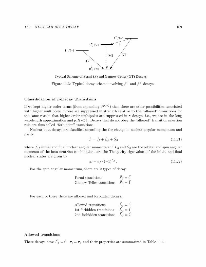
These operators imply that there are selection rules for nuclear beta decay. The Fermi matrixelement is a scalar under rotations and does not change parity. Thus for Fermi (F) transitions wemust have no change in angular momentum (∆J = 0 or Jf = Ji) and no parity change (∆π = 0 orπf = πi). These transitions only occur between states of an isotopic multiplet, connected by theisospin raising operator T+. For Gamow-Teller (GT) transitions, the operator is a vector underrotations and also there is no parity change (∆J = 0, 1 or Jf = Ji ± 1, and ∆π = 0). If Ji 6= 0 thenone could also have Jf = Ji for GT transitions. These selection rules for F and GT decays togetherdefine the class of decays known as “allowed” transitions. The typical decay scheme is shown inFigure 11.3.


+, T=1

1+, T=1

1+, T=1

+0 , T=0

1

GT

Typical Scheme of Fermi (F) and Gamow-Teller (GT) Decays

M1

F

GT

Figure 11.3: Typical decay scheme involving β− and β+ decays.

Classification of β-Decay Transitions

If we kept higher order terms (from expanding ei~pe·~re) then there are other possibilities associatedwith higher multipoles. These are suppressed in strength relative to the “allowed” transitions forthe same reason that higher order multipoles are suppressed in γ decays, i.e., we are in the longwavelength approximation and peR≪ 1. Decays that do not obey the “allowed” transition selectionrule are thus called “forbidden” transitions.

Nuclear beta decays are classified according the the change in nuclear angular momentum andparity.

~Ji = ~Jf + ~Lβ + ~Sβ (11.21)

where ~Ji,f initial and final nuclear angular momenta and Lβ and Sβ are the orbital and spin angularmomenta of the beta-neutrino combination. are the The parity eigenvalues of the initial and finalnuclear states are given by

πi = πf · (−1)Lβ . (11.22)

For the spin angular momentum, there are 2 types of decay:

Fermi transitions ~Sβ = ~0

Gamow-Teller transitions ~Sβ = ~1

For each of these there are allowed and forbidden decays:

Allowed transitions ~Lβ = ~0

1st forbidden transitions ~Lβ = ~1

2nd forbidden transitions ~Lβ = ~2

Allowed transitions

These decays have ~Lβ = 0. πi = πf and their properties are summarized in Table 11.1.


Fermi-type (~Sβ = ~0) Gamow-Teller type ~Sβ = ~1

~Ji = ~Jf~Ji = ~Jf +~1

|∆J | = 0 |∆J | = 0, 1 : no 0+ → 0+

0+ → 0+ : superallowed 0+ → 1+: unique Gamow-Teller

Table 11.1: Properties of allowed beta transitions.

1st forbidden transitions

These decays have ~Lβ = ~1, πi = −πf and the properties listed in Table 11.2.

Fermi-type (~Sβ = ~0) Gamow-Teller type (~Sβ = ~1)

~Ji = ~Jf +~1 ~Ji = ~Jf + ~1 +~1︸︷︷︸

~0, ~1, ~2

|∆J | = 0, 1 3 types:no 0− → 0+ (i) |∆J | = 0

(ii)|∆J | = 0, 1; no 0− → 0+

(iii) |∆J | = 0, 1, 2; no 0− → 0+

no 1+ → 0−

no 12

+ → 12

−

Table 11.2: Properties of first forbidden beta transitions.

Decay Rates

We may now compute the total decay rate (integrate over dEe) to obtain

ω =|Mfi|2m5

e

2π3h7

1

m5e

∫ E0

me

F (Z, E) (E0 −E)2pEdE . (11.23)

We then define the Fermi Integral

f(E0, Z) ≡ 1

m5e

∫ E0

me

F (Z, E) (E0 − E)2pEdE (11.24)

which are standard tabulated functions. In the limit Z → 0, me ≪ E0 we can use the simpleapproximation

f =1

m5e

∫ E0

0E2(E0 − E)2dE =

E50

30m5e

(11.25)

Therefore, we roughly expect ω ∝ E50 and the decay rate is a rather strong function of the available

energy.


The decay rate is related to the half-life t1/2 by

ω =ln2

t1/2=

|Mfi|2m5ef

2π3h7 (11.26)

and it is customary to define the “comparative half-life” or “ft1/2-value” as

ft1/2 ≡ 2π3h7ln2

|Mfi|2m5e

. (11.27)

This comparative half-life is related to simple matrix elements and fundamental constants only:

ft1/2 =2π3h7ln2

G2m5e

[M2

F + g2AM

2GT

] =6221 sec

M2F + g2

AM2GT

. (11.28)

As a common example, we consider a 0+(T = 1,MT = −1) → 0+(T = 1,MT = 0) transition,where the initial and final states are isospin analog states. Then MGT = 0 and only MF contributes.The Fermi matrix element is easily evaluated and we find

MF = 〈T = 1,MT = 0|T+|T = 1,MT = −1〉 (11.29)

=√

T (T + 1) −MT (MT + 1) =√

2

M2F = 2 (11.30)

ft1/2 =6221

2∼= 3110

logft1/2 = 3.5 . (11.31)

Such a strong transition with logft1/2 < 3.7 is termed “superallowed”. Generally these are Fermitransitions.

Parity Nonconservation

The classic demonstration that parity is not conserved by the weak interaction involves the processof nuclear beta decay. One begins by preparing a polarized initial nucleus (e.g. initial spins alignedalong +z). The rate of β emission relative to the spin direction (z) is measured. The rate as afunction of the angle relative to the spin direction J is given by

dω ∝(

1 + αJ · ~Pe

Ee

)

. (11.32)

The quantity J · ~Pe is a pseudoscalar, and the fact that the rate depends on this pseudoscalar mustbe due to the fact that parity symmetry is not conserved by the decay process.

Example (1): 60Co at 0.01 inside solenoid at high B field.The nuclear polarization is ∝ µB

kT . One measures the angular distribution of β− emission relativeto the B-field direction. Experimentally, the value of α = −1 is measured. This indicates thatthe β− is preferentially emitted opposite to the J direction. The explanation is that the parity


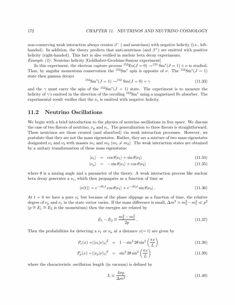
non-conserving weak interaction always creates β− ( and neutrinos) with negative helicity (i.e., left-handed). In addition, the theory predicts that anti-neutrinos (and β+) are emitted with positivehelicity (right-handed). This fact is also verified in nuclear beta decay experiments.Example (2): Neutrino helicity [Goldhaber-Grodzins-Sunyar experiment]

In this experiment, the electron capture process 152Eu(J = 0) →152 Sm∗(J = 1) + ν is studied.Thus, by angular momentum conservation the 152Sm∗ spin is opposite of ν. The 152Sm∗(J = 1)state then gamma decays

152Sm∗(J = 1) →152 Sm(J = 0) + γ (11.33)

and the γ must carry the spin of the 152Sm∗(J = 1) state. The experiment is to measure thehelicity of γ’s emitted in the direction of the recoiling 152Sm∗ using a magnetized Fe absorber. Theexperimental result verifies that the νe is emitted with negative helicity.

11.2 Neutrino Oscillations

We begin with a brief introduction to the physics of neutrino oscillations in free space. We discussthe case of two flavors of neutrino, νµ and νe. The generalization to three flavors is straightforward.These neutrinos are those created (and absorbed) via weak interaction processes. However, wepostulate that they are not the mass eigenstates. Rather, they are a mixture of two mass eigenstatesdesignated ν1 and ν2 with masses m1 and m2 (m1 6= m2). The weak interaction states are obtainedby a unitary transformation of these mass eigenstates:

|νe〉 = cos θ|ν1〉 + sin θ|ν2〉 (11.34)

|νµ〉 = − sin θ|ν1〉 + cos θ|ν2〉 (11.35)

where θ is a mixing angle and a parameter of the theory. A weak interaction process like nuclearbeta decay generates a νe, which then propagates as a function of time as

|ν(t)〉 = e−iE1t cos θ|ν1〉 + e−iE2t sin θ|ν2〉 . (11.36)

At t = 0 we have a pure νe but because of the phase slippage as a function of time, the relativedegree of νµ and νe in the state vector varies. If the mass difference is small, ∆m2 ≡ m2

2−m21 ≪ p2

(p ∼= E1∼= E2 is the momentum) then the energies are related by

E1 −E2∼= m2

2 −m21

2p. (11.37)

Then the probabilities for detecting a νe or νµ at a distance x(= t) are given by

Pe(x) =|〈νe|ν〉t|2 = 1 − sin2 2θ sin2(πx

L

)

(11.38)

Pµ(x) =|〈νµ|ν〉t|2 = sin2 2θ sin2(πx

L

)

(11.39)

where the characteristic oscillation length (in vacuum) is defined by

L ≡ 4πp

∆m2. (11.40)

11.2. NEUTRINO OSCILLATIONS 173

Figure 11.4: Distribution of observed atmospheric neutrino events vs. zenith angle from the Su-perKamiokande experiment, compared with Monte Carlo simulations. The blue hatched regionrepresents the prediction without neutrino oscillations and the red line includes the effect neutrinooscillations. (PC means ‘partially contained’ events.)

This two flavor approximation is a useful approximation for analysis of many experiments. Thegeneralization to three generations involves a 3 × 3 mixing matrix:

|νℓ〉 =∑

i

Uℓi|νi〉 (11.41)

where ℓ is a flavor index (e, µ, τ) and i corresponds to the mass eigenstate (i = 1, 2, 3). The mixingmatrix is usually parametrized by three angles, conventionally denoted as θ12, θ13, θ23, one CPviolating phase δ and two Majorana phases α1, α2. Using c for the cosine and s for the sine, wewrite U as

νe

νµ

ντ

=

c12c13 s12c13 s13e−iδ

−s12c23 − c12s23s13eiδ c12c23 − s12s23s13e

iδ s23c13s12s23 − c12c23s13e

iδ −c12s23 − s12c23s13eiδ c23c13

eiα1/2 ν1

eiα2/2 ν2

ν3

. (11.42)

Here, for example s12 = sin θ12 and so on. There are 3 corresponding mass differences ∆m212,

∆m213 and ∆m2

23. This matrix is analagous to the CKM matrix used to describe the charged weakinteractions of the quarks.

The first experimental observation of neutrino oscillations was due to the SuperKamiokandeexperiment, located deep underground in Japan. This large (22 kTon) water Cerenkov detector


20 30 40 50 60 70 800

0.2

0.4

0.6

0.8

1

1.2

1.4

(km/MeV)eν/E0L

Rat

io

2.6 MeV promptanalysis threshold

KamLAND databest-fit oscillationbest-fit decay

best-fit decoherence

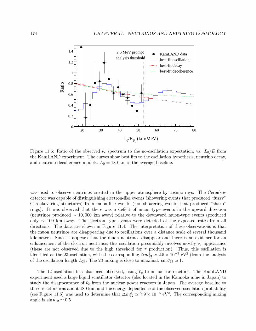
Figure 11.5: Ratio of the observed νe spectrum to the no-oscillation expectation, vs. L0/E fromthe KamLAND experiment. The curves show best fits to the oscillation hypothesis, neutrino decay,and neutrino decoherence models. L0 = 180 km is the average baseline.

was used to observe neutrinos created in the upper atmosphere by cosmic rays. The Cerenkovdetector was capable of distinguishing electron-like events (showering events that produced “fuzzy”Cerenkov ring structures) from muon-like events (non-showering events that produced “sharp”rings). It was observed that there was a deficit of muon type events in the upward direction(neutrinos produced ∼ 10, 000 km away) relative to the downward muon-type events (producedonly ∼ 100 km away. The electron type events were detected at the expected rates from alldirections. The data are shown in Figure 11.4. The interpretation of these observations is thatthe muon neutrinos are disappearing due to oscillations over a distance scale of several thousandkilometers. Since it appears that the muon neutrinos disappear and there is no evidence for anenhancement of the electron neutrinos, this oscillation presumably involves mostly ντ appearance(these are not observed due to the high threshold for τ production). Thus, this oscillation isidentified as the 23 oscillation, with the corresponding ∆m2

23 ≃ 2.5 × 10−3 eV2 (from the analysisof the oscillation length L23. The 23 mixing is close to maximal: sin θ23 ≃ 1.

The 12 oscillation has also been observed, using νe from nuclear reactors. The KamLANDexperiment used a large liquid scintillator detector (also located in the Kamioka mine in Japan) tostudy the disappearance of νe from the nuclear power reactors in Japan. The average baseline tothese reactors was about 180 km, and the energy dependence of the observed oscillation probability(see Figure 11.5) was used to determine that ∆m2

12 ≃ 7.9 × 10−5 eV2. The corresponding mixingangle is sin θ12 ≃ 0.5

11.3. MATTER ENHANCED OSCILLATIONS 175

11.3 Matter Enhanced Oscillations

In dense matter (like the solar interior), there is a substantial density of electrons present. The νe

interact with electrons differently than do the νµ. This affects the phase slippage of νe relative toνµ and can have a dramatic effect on the flavor transformation dynamics.

It is useful to recast the oscillation formulae in a matrix form as follows. (We will simplifythis discussion to just 2 flavors.) The transformation between basis states can be written (C ≡cos θ, S ≡ sin θ)

(νe

νµ

)

=

(C S−S C

) (ν1

ν2

)

(11.43)

with the inverse transformation

(ν1

ν2

)

=

(C −SS C

) (νe

νµ

)

. (11.44)

The time evolution of the mass eigenstates can be written

|νi(t)〉 = e−i(Ei−p)t|νi(0)〉 (11.45)

= e−im2it/2p|νi(0)〉; i = 1, 2, (11.46)

or

d|νi〉dt

= −im2i

2p|νi〉. (11.47)

Therefore, we can express the time evolution in the νe, νµ basis as

id

dt

(νe

νµ

)

=

(C S−S C

)

id

dt

(ν1

ν2

)

(11.48)

=1

2p

(C S−S C

)(m2

1 00 m2

2

)(ν1

ν2

)

(11.49)

=1

2p

(C2m2

1 + S2m22 CS∆m2

CS∆m2 C2m22 + S2m2

1

)(νe

νµ

)

. (11.50)

The effect of dense matter is then included by modifying the diagonal matrix element

C2m21 + S2m2

2 → C2m21 + S2m2

2 + 2√

2GFnep (11.51)

where ne is the number of e− per unit volume. If we now define

L0 ≡ 2π√2GFne

(11.52)

the solutions (for fixed ne) can be rewritten as

|〈νe|ν(t)〉|2 = 1 − sin2 2θm sin2 πx

Lm(11.53)

|〈νµ|ν(t)〉|2 = sin2 2θm sin2 πx

Lm(11.54)


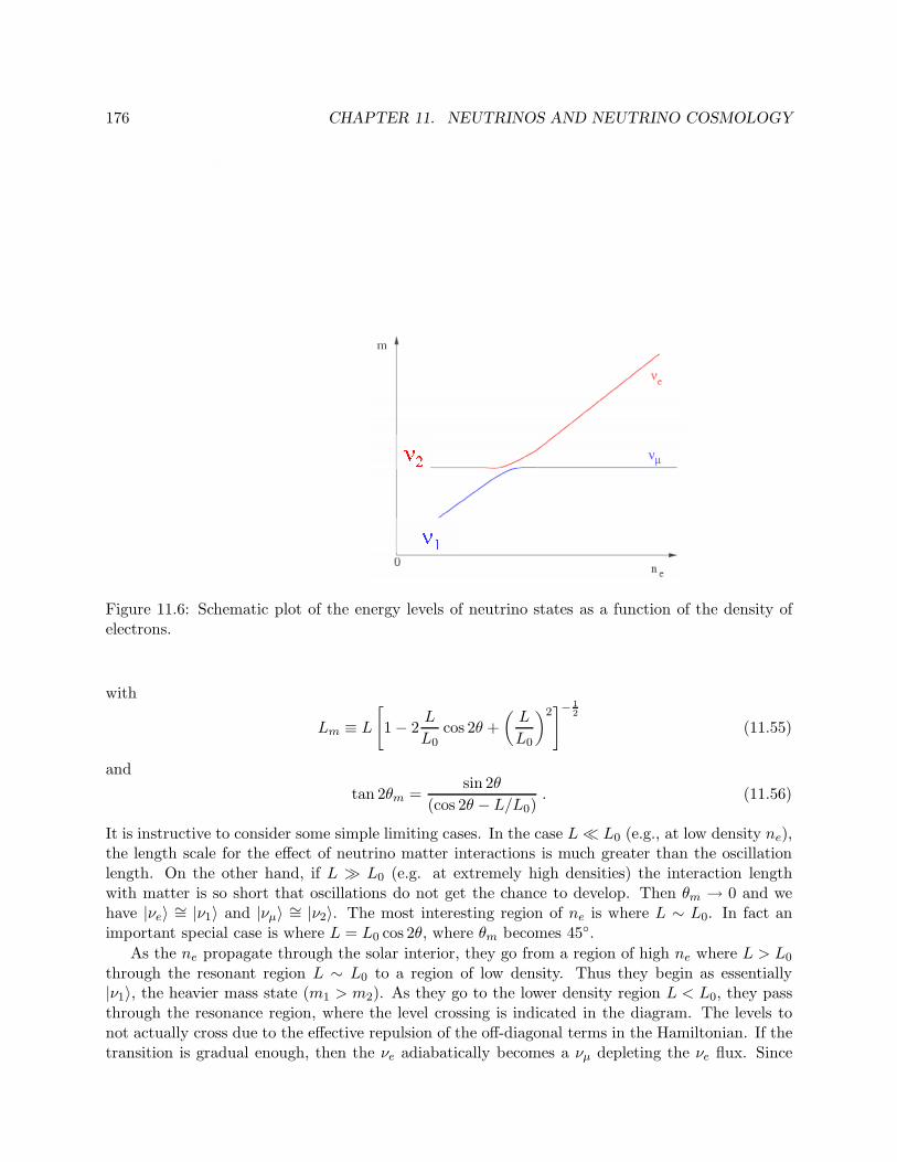
Figure 11.6: Schematic plot of the energy levels of neutrino states as a function of the density ofelectrons.

with

Lm ≡ L

[

1 − 2L

L0cos 2θ +

(L

L0

)2]− 1

2

(11.55)

and

tan 2θm =sin 2θ

(cos 2θ − L/L0). (11.56)

It is instructive to consider some simple limiting cases. In the case L≪ L0 (e.g., at low density ne),the length scale for the effect of neutrino matter interactions is much greater than the oscillationlength. On the other hand, if L ≫ L0 (e.g. at extremely high densities) the interaction lengthwith matter is so short that oscillations do not get the chance to develop. Then θm → 0 and wehave |νe〉 ∼= |ν1〉 and |νµ〉 ∼= |ν2〉. The most interesting region of ne is where L ∼ L0. In fact animportant special case is where L = L0 cos 2θ, where θm becomes 45.

As the ne propagate through the solar interior, they go from a region of high ne where L > L0

through the resonant region L ∼ L0 to a region of low density. Thus they begin as essentially|ν1〉, the heavier mass state (m1 > m2). As they go to the lower density region L < L0, they passthrough the resonance region, where the level crossing is indicated in the diagram. The levels tonot actually cross due to the effective repulsion of the off-diagonal terms in the Hamiltonian. If thetransition is gradual enough, then the νe adiabatically becomes a νµ depleting the νe flux. Since

11.4. DOUBLE BETA DECAY 177

the expression for L/L0 is momentum dependent

L

L0=

2√

2GFnep

∆m2(11.57)

the conversion νe → νµ is energy dependent. In fact, if the value of ∆m2 is about right then thelow energy neutrinos have L/L0 ≪ 1 in the solar interior and only the higher energy neutrinosundergo a transformation.

This explanation was dramatically verified by the Sudbury Neutrino Observatory (SNO) ex-periment. The SNO experiment combines the now high-developed capability of water Cerenkovdetectors with the unique opportunities afforded by using deuterium to detect the solar neutrinos[?, ?]. Low energy neutrinos can dissociate deuterium via the charged current (CC) reaction

νe + d→ e− + 2p (11.58)

or the neutral current (NC) reaction

νℓ + d→ νℓ + p+ n . (11.59)

Only νe can produce the CC reaction, but all flavors ℓ = e, µ, τ can contribute to the NC rate.The CC reaction is detected via the energetic spectrum of e− which closely follows the 8B solarνe spectrum. The NC reaction involves three methods for detection of the produced neutron: (a)capture on deuterium and detection of the 6.25 MeV γ-ray, (b) capture on Cl (due to salt added tothe D2O) and detection of the 8.6 MeV γ-ray, or (c) capture in 3He proportional counters immersedin the detector. There are also some events associated with the elastic scattering of the solar-νon e− in the detector which is dominated by the charged current reaction (again only νe) but hassome ∼ 20% contribution from neutral currents (all flavors equally contribute).

The SNO collaboration has published data on the CC and NC rate (from processes (a) and(b)). Additional data from the NC process (c) will be forthcoming in the future. Nevertheless, thereported results (see Fig. 11.7) demonstrate very clearly that the total neutrino flux (νe + νµ + ντ

as determined from NC) is in good agreement with the SSM, but that the νe flux is suppressed (asdetermined from CC). This represents rather definitive evidence that the νe suppression is due toflavor-changing processes that convert the νe to the other flavors, as expected from ν-oscillations.The SNO results can be combined with the other solar neutrino data to provide constraints on theparameters θ12 and ∆m2

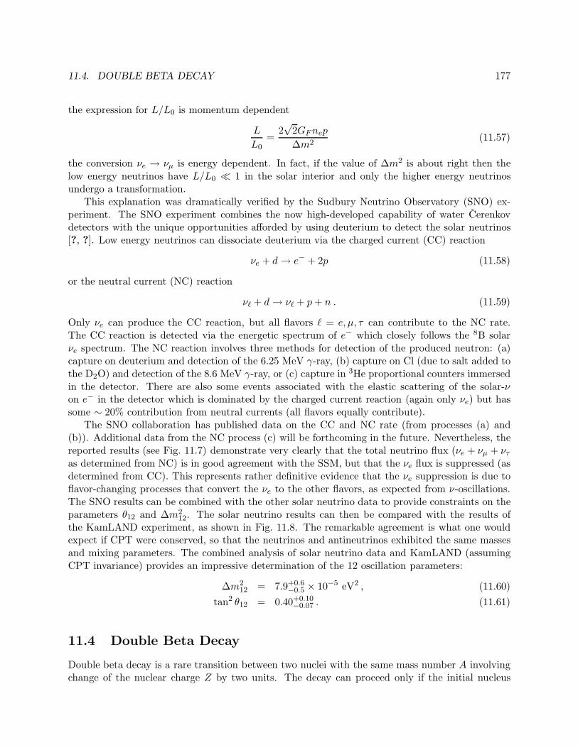
12. The solar neutrino results can then be compared with the results ofthe KamLAND experiment, as shown in Fig. 11.8. The remarkable agreement is what one wouldexpect if CPT were conserved, so that the neutrinos and antineutrinos exhibited the same massesand mixing parameters. The combined analysis of solar neutrino data and KamLAND (assumingCPT invariance) provides an impressive determination of the 12 oscillation parameters:

∆m212 = 7.9+0.6

−0.5 × 10−5 eV2 , (11.60)

tan2 θ12 = 0.40+0.10−0.07 . (11.61)

11.4 Double Beta Decay

Double beta decay is a rare transition between two nuclei with the same mass number A involvingchange of the nuclear charge Z by two units. The decay can proceed only if the initial nucleus


Figure 11.7: Measured solar neutrino fluxes from SNO for the NC and CC processes, along withelastic scattering events (ES) and the standard solar model prediction .

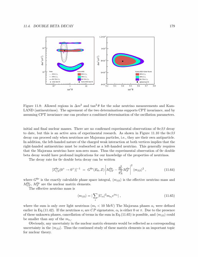
is less bound than the final one, and both must be more bound than the intermediate nucleus.These conditions are fulfilled in nature for many even-even nuclei, due to the nature of the pairinginteraction as discussed in Chapter 9. Fig. 11.9 shows a typical situation for A = 136. Typically,the decay can proceed from the ground state (spin and parity always 0+) of the initial nucleus tothe ground state (also 0+) of the final nucleus, although the decay into excited states (0+ or 2+) isin some cases also energetically possible.

There are, in principle, two types of double beta decay: 2νββ where 2 neutrinos and 2 β particlesare emitted in the final state, and 0νββ where only the 2 β particles are emitted. The two-neutrinodecay, 2νββ,

(Z,A) → (Z + 2, A) + e−1 + e−2 + νe1 + νe2 (11.62)

conserves not only electric charge but also lepton number. On the other hand, the neutrinolessdecay,

(Z,A) → (Z + 2, A) + e−1 + e−2 (11.63)

violates lepton number conservation. One can distinguish the two decay modes by the shape ofthe electron sum energy spectra, which are determined by the phase space of the outgoing lightparticles. Since the nuclear masses are so much larger than the decay Q value, the nuclear recoilenergy is negligible, and the electron sum energy of the 0νββ is simply a peak at Te1 + Te2 = Qsmeared only by the detector resolution.

The 2νββ decay is an allowed process with a very long lifetime ∼ 1020 years, and has now beenexperimentally observed in several nuclei cases. This is a standard second order weak interactionprocess, and is a significant challenge for nuclear theory to calculate the lifetimes.

The 0νββ decay involves a vertex changing two neutrons into two protons with the emission oftwo electrons and nothing else. The total energy of the two electrons is a constant determined by the

11.4. DOUBLE BETA DECAY 179

)2 (

eV2

m∆

-510

-410

θ 2tan

-110 1 10

KamLAND

95% C.L.

99% C.L.

99.73% C.L.

KamLAND best fit

Solar

95% C.L.

99% C.L.

99.73% C.L.

solar best fit

θ 2tan

0.2 0.3 0.4 0.5 0.6 0.7 0.8

)2 (

eV2

m∆

KamLAND+Solar fluxes

95% C.L.

99% C.L.

99.73% C.L.

global best fit-510×4

-510×6

-510×8

-410×1

-410×1.2

Figure 11.8: Allowed regions in ∆m2 and tan2 θ for the solar neutrino measurements and Kam-LAND (antineutrinos). The agreement of the two determinations supports CPT invariance, and byassuming CPT invariance one can produce a combined determination of the oscillation parameters.

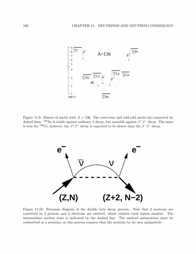
initial and final nuclear masses. There are no confirmed experimental observations of 0νββ decayto date, but this is an active area of experimental research. As shown in Figure 11.10 the 0νββdecay can proceed only when neutrinos are Majorana particles, i.e., they are their own antiparticle.In addition, the left-handed nature of the charged weak interaction at both vertices implies that theright-handed antineutrino must be reabsorbed as a left-handed neutrino. This generally requiresthat the Majorana neutrino have non-zero mass. Thus the experimental observation of 0ν doublebeta decay would have profound implications for our knowledge of the properties of neutrinos.

The decay rate for 0ν double beta decay can be written

[T 0ν1/2(0

+ → 0+)]−1 = G0ν(E0, Z)

∣∣∣∣∣M0ν

GT − g2V

g2A

M0νF

∣∣∣∣∣

2

〈mββ〉2 , (11.64)

where G0ν is the exactly calculable phase space integral, 〈mββ〉 is the effective neutrino mass andM0ν

GT , M0νF are the nuclear matrix elements.

The effective neutrino mass is

〈mββ〉 = |∑

i

|Uei|2mνieiαi | , (11.65)

where the sum is only over light neutrinos (mi < 10 MeV) The Majorana phases αi were definedearlier in Eq.(11.42). If the neutrinos νi are CP eigenstates, αi is either 0 or π. Due to the presenceof these unknown phases, cancellation of terms in the sum in Eq.(11.65) is possible, and 〈mββ〉 couldbe smaller than any of the mνi

.Obviously, any uncertainty in the nuclear matrix elements would be reflected as a corresponding

uncertainty in the 〈mββ〉. Thus the continued study of these matrix elements is an important topicfor nuclear theory.


13653 I

Ba

Xe54136 55 Cs136

13656

La13657 Ce136

58

Pr13659

β

β

βββ

β

−

−+

+

(MeV)1

2

3

4

5

6

7

8

9

A=136

Figure 11.9: Masses of nuclei with A = 136. The even-even and odd-odd nuclei are connected bydotted lines. 136Xe is stable against ordinary β decay, but unstable against β−β− decay. The sameis true for 136Ce, however, the β+β+ decay is expected to be slower than the β−β− decay.

ee− −

(Z,N) (Z+2, N−2)

νν

Figure 11.10: Feynman diagram of the double beta decay process. Note that 2 neutrons areconverted to 2 protons and 2 electrons are emitted, which violates total lepton number. Theintermediate nuclear state is indicated by the dashed line. The emitted antineutrino must bereabsorbed as a neutrino, so this process requires that the neutrino be its own antiparticle.

Chapter 12

Supernova, Neutron Star and BlackHole

For a star with mass larger than 10 solar masses, it undergoes all stages of nuclear burning andeventually develops an iron core. As the mass of the iron core reaches Chandrasekhar limit, itbecomes unstable and will collapse under two mechanisms. First, because of the enormous heat,the energy of the photon is high-enough to produce photo-disintegration of iron. Second, theenergy of the electron becomes so large that it is viable to have inverse beta reaction, generatingneutrons and neutrinos. Therefore, the star will rapidly collapses into a neutron star or a blackhole. The gravitational energy released through the processes will produce a huge explosion whichis the supernova type II or Ib. In this Chapter, we discuss the supernova explosion phenomena anddiscuss the heavy nucleus generation, the physics of neutron star and black hole.

12.1 Collapse of a Well-Burned Star into a Neutron Star

When a star is massive enough, after the nuclear burning resulting the iron core, the star cannothave any further nuclear fusion. However, under the gravitational pressure, the star will shrinkfuture, and at some point, it becomes more profitable to turn the protons into neutrons.

Now note that (for a fixed radius r) the electron and gravitational energy of the star increaseswith increasing x for both non-relativistic (NR) and relativistic (Rel) electron gases:

NR : E ∼ x5/3 (12.1)

Rel : E ∼ x4/3. (12.2)

So it is energetically favorable if we can decrease x through the weak process

e− + p→ n+ νe . (12.3)

At large enough density, the Fermi energy of the electrons exceeds the mass difference Mn−Mp

and this process spontaneously proceeds to convert the star to “neutron matter.” For a non-relativistic electron gas, we set the Fermi energy to about 1 MeV and using the expression

EF =h2

2me

(

3π2xn

Ω

)2/3

(12.4)

181

182 CHAPTER 12. SUPERNOVA, NEUTRON STAR AND BLACK HOLE

we obtain the density

n

Ω= 9 × 1030/cm3 (12.5)

ρ ∼= 1.5 × 107 g/cm3. (12.6)

For relativistic electrons EF = 2 MeV implies the density ρ ∼= 108 g/cm3. Thus, for ρ > 108 g/cm3

we expect the protons to convert to neutrons and the star will consist of neutron matter.

We can then write the total energy as the sum of neutron kinetic energy, electron kinetic energy,and the gravitational potential energy:

E(r, x) =3h2(1 − x)n

10Mpr2

(9π(1 − x)n

4

)2/3

+3hxn

4r

(9πxn

4

)1/3

− 3

5Gn2M2

p

r. (12.7)

We then require the following conditions for an equilibrium configuration:

∂E

∂r= 0 (12.8)

∂E

∂x= 0. (12.9)

Assuming that the matter predominantly converts to neutrons we choose x = 0 and obtain theequilibrium radius

req =h2

GnM3p

(9πn

4

)2/3

. (12.10)

For n = 1.2 × 1057 (1 M⊙) we obtain the values

req = 1.24 × 106 cm = 1.24 × 104 m = 1.24 km (12.11)

Ω = 7.96 × 1018 cm3 (12.12)

ρ = 2.5 × 1014 g/cm3 (12.13)

Plugging this req into E(req, x) and requiring

∂E(req, x)

∂x= 0 (12.14)

yields the value x = 0.005. Thus we find a consistent solution with x ∼ 0 and ρ ∼ ρNM with aradius of req ∼ 1 km. This is a large nucleus at nuclear matter density, consisting of neutrons only,with a radius of 1 km!

We now include nuclear interactions and use the parametrization of the Bethe-Weizsacker for-mula:

E

n∼= aA(ρ) − aV (ρ) − 3

5G

[4πM2M4

p

3ρ

]1/3

(12.15)

where we have assumed x = 0 and ρ = nΩ=# nucleons/cm3. We need to consider the two regions

of density:

12.2. SUPERNOVA EXPLOSION AND R-PROCESS 183

• (a) For ρ = ρ0 = 1.4 × 1038/cm3, we know that aA − aV∼= 7.5 MeV=7.5 × 10−3 GeV from

the empirical fits to normal nuclei. This implies a minimum star mass for En < 0

M >1

M2p

(3

4πρ0

)1/3 (5(aA − aV )

3G

)3/2

= 0.04 M⊙ (12.16)

or n = 4.3 × 1055 with r =(

3n4πρ

)1/3= 4 km.

• (b) For ρ > ρ0, we need the ρ dependence of BA = aV − aA.

Empirically (from measurements of the “breathing mode” of nuclei) and from calculations basedon nuclear matter theory (more later) we find the “compressibility”:

K = −k2f

d2(B/A)

dk2f

= −9ρ20

d2(B/A)

dρ2= 0.1 − 0.2 GeV. (12.17)

Using this parameter we can approximately describe the compression of nuclear matter by theexpression

B

A=

(B

A

)

0− K

18ρ20

(ρ− ρ0)2 . (12.18)

Then we obtain the equilibrium condition for neutron star stability as

d

dρ

(E

n

)

=K

9ρ20

ρ− 1

5G

[4πM2M4

p

3ρ2

]1/3

= 0 (12.19)

which yields the density

ρ =

(

9ρ20G

5K

)3/5 (4πM2M4

p

3

)1/5

. (12.20)

If we now take M = 1.5 M⊙ we find

ρ ∼= (1.6 − 2.4) × 1038cm−3 = (1.1 − 1.7)ρ0 . (12.21)

In fact more realistic calculations give ρ ∼ 4− 5 ρ0 and x ∼0.15. Nevertheless, our simple approx-imations do illustrate the basic physical principles of the structure of neutron stars.

12.2 Supernova Explosion and R-process

In Type II supernova, mass flows into the core by the continued making of iron, the most stablenucleus, from nuclear fusion. Once the core has gained so much mass that it cannot withstand itsown weight (Chandrasekar limit), the core implodes. This implosion can usually be brought to ahalt by neutrons, the only things in nature that can stop such a gravitational collapse. When thecollapse is abruptly stopped by the neutrons, matter bounces off the hard iron core, thus turningthe implosion into an explosion, ejecting the star mantle.

Therefore, the supernova explosion is characterized by electron captures and neutrino release.In fact, almost all of the energy of the supernova II and Ib and Ic explosions is released in the


form of the neutrinos. The fundamental problem in understanding the supernova explosion is theenergy transfer process in which the free fall energy transfers into the star mantle and resulting inan explosion. The detailed study shows that it is a very difficult problem. Numerical simulationshave difficulty to create an explosion.

One of the most important function of the supernova explosion is to create heavy elements inthe Universe. These elements cannot be produced in the usual star fusion processes and must beproduced in the unusual environment such as R-process.

The R-process (R for rapid) is a neutron capture process for radioactive elements which occursin high neutron density, high temperature conditions. In the R-process nuclei are bombarded witha large neutron flux to form highly unstable neutron rich nuclei which very rapidly decay to formstable neutron rich nuclei.

A primary site of the R-process is believed to be iron-core collapse supernovae, which providethe necessary physical conditions for the R-process. However, the abundance of R-process elementsrequires that either only a small fraction of supernova return R-process elements to the outside orthat each supernova only contributes a very small amount of R-process elements.

Due to the much higher neutron flux in this process (on the order of 1022 neutrons per cm2 persecond), the rate of isotopic formation is much faster than the beta decays which follow, meaningthat this process ”runs up” along the neutron drip line (a line alone with adding more neutronswill not lead to a stable nucleus) with the only two hold-ups being closed neutron shells extendingthe time it takes to create new isotopes, and the degree of nuclear stability in the heavy-isotoperegion, which terminates the R-process when such nuclei become readily unstable to spontaneousfission (currently believed to be in the region of A = 270 - or roughly in the Rutherfordium -Darmstadtium area of the periodic table).

Elemental abundance peaks show some support for the idea of rapid neutron capture anddelayed beta emission, as the R-process peaks are at about 10 Atomic mass units below those ofthe S-process peaks (which occur exactly at closed neutron shells), indicating that the ”run up”along the neutron drip line reaches closed neutron shells but with sufficient proton deficiency tomake the peaks resolvable.

12.3 Neutron Stars

As the result of the type II and type Ib and Ic supernova explosion, a neutron star forms. Theconcept of a neutron star was suggested by Baade and Zwicky as early as 1933.

A stable neutron star has mass of order 1.35 to 2.1 solar masses, with a radius about 20 to 10km. The density of the neutron stars is exceedingly large, on the order of 1014 to 2 × 1015 g/cm3.

In the core collapsing processes, the angular momentum is almost conserved and therefore, theneutron star has a large angular momentum. Therefore it rotates several times or even hundreds oftimes a second. However, the rotational axis needs not coincide with the axis of magnetic field. Assuch, when it rotates, it produces electromagnetic radiation. This radiation is powered by rotationand hence the star is also called ”rotation powered pulsar”. As the star rotation, one sees a periodicemission of the radiation in one directions. As the radiation carries away the rotational energy, therotation slows down. However, this process takes a very very long time.

Some of the most interesting questions about the neutron stars have not been settled, whichinclude what is the maximum mass of a neutron star? What is the radius of a neutron star of agiven mass, and what is the physical origin of transient phenomena in neutron star?

12.4. BLACK HOLES 185

The maximum mass of a neutron star is a result of gravitational attraction and nuclear repulsion.Since the largest mass star corresponds to a largest nuclear density, this also yields what is thelargest nuclear density possible in a star without gravitational collapse. This upper limit clearlyindicates a particular class of equation of states for neutron-rich nuclear matter.

Besides the maximum mass, the radius of the neutron star also depends on the equation ofstate.

For a piece of matter without the problem of gravitational collapse, the ground state of coldmatter at extremely high-density might be a color superconductor in a color-flavor-locked phase.

Density dependence of the symmetry energy is an important piece of information characteriz-ing the equation of state for neutron-rich matter. This density dependence might be measurablethrough measuring the neutron radius of Pb nucleus. Through parity elastic electron scattering onthe Pb nucleus, one might be able to learn the density dependence of the symmetry energy.

12.4 Black Holes

When the mass of a neutron star exceeds a certain limit, the degenerate pressure of the neutronsno longer can resist the gravitational pull and the star will continue to collapse to form a blackhole. The size of the black hole is determined by its Schwartzschild radius,

R = 2GM/c2 (12.22)

which is proportional to its mass. One way to derive this to calculate the escape velocity of anobject at distance r,

1

2mv2 = GmM/r (12.23)

At the Schwartzschild radius R, the escape velocity equals to the speed of light c. Because of that,even light cannot escape the gravitational pull of a black hole.

As an example, a blackhole with one solar mass has a Schwartzschild radius 3km! A blackholeof 50kg mass has a radius 10−10 fm!

Other interesting phenomena associated with black holes include 1) speeding up of the clock asit co-moves with the surface of the collapsing star and 2) the redshift of a photon to zero frequency.

A possible way to observe a black hole is binary systems in which one of them is a neutron starand the other is a black hole. As the mass of the neutron star being sucked into a black hole, thereis an X-ray emission. One of the candidate is Cygnus X-1. Another place to look for black holesis at the centers of the galaxies. The center of the Milky Way might contain a black hole of mass4 × 106 solar masses.

Black hole has temperature. The so-called Hawking temperature of a black hole is

kTH =hc3

8πGM(12.24)

which is inversely proportional to its mass. Larger the mass, lower the temperature. Because ofthis, the black hole has also entropy, which is proportional to its surface area.

An object with finite temperature will radiate according to the black-body radiation formula—itis called Hawking radiation in this context. When it radiates, the mass of the black hole decreases,


and its temperature increases, and eventually all masses radiate away. Therefore, a black hole whenleft along has a finite life time. It is not difficult to show that the life time of a black hole is

∼ G2M3/hc4 (12.25)

which is a very long time for a blackhole of one solar mass.

Documents

Structure of Finite Nuclei - UMD Physics · Chapter 8 Structure of Finite Nuclei The nuclear shell model, developed by Mayer and Jensen in 1952, is now a very successful and highly