HAL Id: hal-01037972https://hal.archives-ouvertes.fr/hal-01037972

Submitted on 23 Jul 2014

HAL is a multi-disciplinary open accessarchive for the deposit and dissemination of sci-entific research documents, whether they are pub-lished or not. The documents may come fromteaching and research institutions in France orabroad, or from public or private research centers.

L’archive ouverte pluridisciplinaire HAL, estdestinée au dépôt et à la diffusion de documentsscientifiques de niveau recherche, publiés ou non,émanant des établissements d’enseignement et derecherche français ou étrangers, des laboratoirespublics ou privés.

Structure tensor based analysis of cells and nucleiorganization in tissues

Wenxing Zhang, Jérôme Fehrenbach, Annaick Desmaison, Valérie Lobjois,Bernard Ducommun, Pierre Weiss

To cite this version:Wenxing Zhang, Jérôme Fehrenbach, Annaick Desmaison, Valérie Lobjois, Bernard Ducommun, etal.. Structure tensor based analysis of cells and nuclei organization in tissues. IEEE Transactions onMedical Imaging, Institute of Electrical and Electronics Engineers, 2016, �10.1109/TMI.2015.2470093�.�hal-01037972�

Structure tensor based analysis of cells and

nuclei organization in tissues

Wenxing Zhang1,2,3, Jérôme Fehrenbach1,2,4,5, Annaïck

Desmaison1,2, Valérie Lobjois1,2, Bernard Ducommun1,2,6, and

Pierre Weiss ∗1,2,4,5

1CNRS, ITAV-USR3505, Toulouse, France.2Université de Toulouse, ITAV-USR3505, Toulouse, France.

3School of Mathematical Sciences, University of Electronic Science

and Technology of China, Chengdu, China.4CNRS, IMT-UMR5219, Toulouse, France.

5Université de Toulouse, IMT-UMR5219, Toulouse, France.6CHU de Toulouse, Toulouse, France.

July 23, 2014

Abstract

Motivation: Extracting geometrical information from large 2D or 3D

biomedical images is important to better understand fundamental phe-

nomena such as morphogenesis. We address the problem of automatically

analyzing spatial organization of cells or nuclei in 2D or 3D images of

tissues. This problem is challenging due to the usually low quality of

microscopy images as well as their typically large sizes.

Results: The structure tensor is a simple and robust descriptor that

was developed to analyze textures orientation. Contrarily to segmentation

methods which rely on an object based modelling of images, the structure

tensor views the sample at a macroscopic scale, like a continuum. We

propose an original theoretical analysis of this tool and show that it allows

quantifying two important features of nuclei in tissues: their privileged

orientation as well as the ratio between the length of their main axes. A

quantitative evaluation of the method is provided for synthetic and real 2D

and 3D images. As an application, we analyze the nuclei orientation and

anisotropy on multicellular tumor spheroids cryosections. This analysis

reveals that cells are elongated in a privileged direction that is parallel to

the boundary of the spheroid.

Availability: Source codes are available at

http://www.math.univ-toulouse.fr/~weiss/

∗Corresponding author: pierre.armand.weiss@gmail.com

1

1 Introduction

The advent of new imaging technologies allows observing biological samples withan unprecedented spatial, temporal and spectral resolution. It offers new op-portunities to perform systematic studies of geometrical configurations of cellsor nuclei in their micro-environment to better understand the fundamental pro-cesses involved in morphogenesis or tumor growth [22, 18].

Due to the huge amount of data contained in large images, automatic pro-cedures are however essential to assess cells properties such as location, size,orientation, aspect ratio, etc... The lack of robust, fast and universal proceduresto provide such a geometric description is probably one of the main obstaclesto exploit the full potential of images.

The mainstream approach to analyze image contents nowadays consists insegmenting each cell/nuclei independently [22, 24]. A precise segmentation com-pletely describes the geometrical contents of images and is often regarded as thebest source of information one can hope for. However biological images oftensuffer from many degradations. For instance, in fluorescence microscopy, lightscattering, absorption or poor signal to noise ratio strongly impair image qual-ity, especially in 3D. In many situations it is therefore hopeless to perform aproper image segmentation. Moreover, in cases where large cell populations areinvestigated, a complete segmentation (i.e. a precise description of the objectsboundaries) still brings more information than needed to understand the overallgeometrical distribution.

In this paper we therefore pursue a somehow less ambitious goal. We adopta macroscopic point of view and consider the biological sample as a continuousmedium. This idea stems from mathematical models that describe tissues ascontinuous media such as incompressible fluids, elastic or viscoelastic materials[6, 1, 17, 16, 4]. Our main contribution is to show through both theoretical andnumerical results that the so-called structure tensor [12, 3, 13], provides a fast,robust and precise enough tool to retrieve cells orientation and anisotropy in2D and in 3D. We show the following original results:

• While the structure tensor is usually implemented to assess texture orien-tations, we show that it also allows quantifying precisely the anisotropyof cells or nuclei. This is done by analyzing the method behavior on fieldsof functions with ellipsoidal isosurfaces.

• The proposed mathematical analysis also allows quantifying the methodbias. It shows that a very good estimation can be expected even whenvery few nuclei are locally similar (in the sense that they can be wellapproximated by the same ellipsoid).

• We show that the method is invariant under contrast changes.

We also perform various experiments to validate our theoretical findings. Weassess the structure tensor efficiency on synthetic and real 2D and 3D images.Its output is compared to ground-truth obtained analytically in case of syntheticdata or manually in case of real data. These comparisons show that the structuretensor allows to quickly assess cells organization at a large scale. We finish thepaper by providing an example of application to the analysis of geometricalconfigurations of nuclei in multicellular tumor spheroids.

2

Related work The structure tensor has already been used in various contextsof biological imaging. One of its main applications is coherence enhancing ordiffusion [33, 34, 24] which usually allows improving images quality withoutdegrading their geometrical content too much. It was also used to analyzegeometrical features such as fibers orientations in 2D and 3D [23, 20, 10, 26, 11].The works [26, 11] also come with an ImageJ plugin http://bigwww.epfl.

ch/demo/orientation/. This plugin has a nice interface and can be used toreproduce some experiments of our paper. The authors of these two referencesmention that the structure tensor allows quantifying the orientation and theisotropy properties of a region of interest. However, the isotropy is defined ina way different from the present paper and the authors do not state preciselyhow this information relates to the image contents.

Paper organization The rest of the paper is organized as follows. Notationis introduced in Section 2. Section 3 constitutes the theoretical part of thepaper. We introduce the structure tensor and demonstrate its properties whenapplied to images that consist in fields of functions with ellipsoidal isosurfaces.In Section 4, we illustrate the method on synthetic and real 2D and 3D data.

2 Notation

For any x, y ∈ Rd, the angle in degrees between x and y is denoted ∠(x, y), thisangle lies in [0◦, 90◦]. The ℓp-norm of x ∈ Rd is denoted ‖x‖p and defined by

‖x‖p := (∑d

i=1 |xi|p)1/p. The positive semidefiniteness of a matrix A is denoted

A � 0. The spectral norm of a matrix A is denoted ‖A‖2. We denote A :=A/‖A‖2 the normalized version of A. The largest (resp. smallest) eigenvalueof A is denoted λmax(A) (resp. λmin(A)). The notation Id denotes the identityoperator. Given a vector x ∈ Rd, we let diag(x) denote a diagonal matrixwhose diagonal elements are the entries of x. The Givens transform, denotedby Rθ

ij ∈ Rd×d, represents a counter-clockwise rotation for an angle θ in the

(i, j)-coordinates plane. In the particular case d = 2, it is abbreviated Rθ.

3 Theoretical analysis

The structure tensor appeared in the field of image processing in the late 80’s [12]for the problem of interest point detection. It was then justified theoretically andpopularized in different contexts such as interest point detection [12, 15], textureanalysis [3, 13], representation of flow-like images [25], optical flow problems [19]and anisotropic or coherence enhancing diffusion [24, 33, 34].

In this section, we first recall the definition of structure tensor, then showits capability of analyzing fields of locally coherent ellipses (in 2D) or ellipsoids(in 3D). The motivation for introducing fields of ellipses is that images such asFigure 3 are a rather good approximation of certain dense tissues such as mi-crotumors. To the best of our knowledge, even though fields of locally coherentellipsoids share some similarities with flow-like images, the proposed theoreticalanalysis and results are original and shed a novel light on the structure tensor.

3

3.1 Preliminary facts about the structure tensor

Let u : Rd → R denote a grayscale image. In this paper, we restrict on thepractical cases d = 2 and d = 3, although the theory is valid in any dimension.For ease of exposition, we assume that u ∈ C1(Rd) and has bounded partialderivatives. The function K ∈ L1(Rd) is a filter that satisfies the followingconditions:

(i) K(x) ≥ 0, ∀x ∈ Rd; (ii)

∫

Rd

K(x) dx = 1. (1)

For any ρ > 0, we define Kρ the scaled version of K by

Kρ(x) :=1

ρdK

(x

ρ

), ∀x ∈ R

d. (2)

The conditions (1) still hold for any ρ > 0. In practice, K is usually a smoothingfilter (e.g. a Gaussian) and Kρ is a scaled version at scale ρ.

The structure tensor of u, denoted by Jρ, is defined by

Jρ := Kρ ⋆(∇u∇uT

), (3)

where ∇ denotes the gradient operator and ‘⋆’ is the convolution operationwhich acts independently on each component of the d×d tensor ∇u∇uT . Usingthe boundedness of the partial derivatives of u and the conditions (1), we have

| (Jρ(x))i,j | ≤

(∫

Rd

|Kρ(x− y)| dy

)

︸ ︷︷ ︸=1

(maxy∈Rd

|(∂iu∂ju)(y)|

)< +∞

for any x ∈ Rd, which implies that Jρ is bounded in Rd. Notice that thedefinition given in equation (3) differs slightly from that found in standardarticles or textbooks such as [33, 34]. Therein, the image u is first convolvedwith a Gaussian filter and the filter K is assumed to be a Gaussian, see thediscussion in Section 3.4.

A useful property of structure tensor is its positive semidefiniteness, which isa direct consequence of (1) and the convexity of the cone of symmetric positivesemidefinite matrices.

Proposition 1 (Positive semidefiniteness) The structure tensor satisfies Jρ(x) �0 for any ρ > 0 and any x ∈ Rd.

3.2 Structure tensor and a single ellipsoid

In this section, we analyze the structure tensor behavior on a simple imagewhose isosurfaces are concentric ellipsoids. We show that it allows recoveringits principal orientations as well as the ratios between the length of the ellipsoidmain axes.

Let ϕ : R+ → R denote a C1 function different from 0 satisfying ϕ′(0) =0. Let A ∈ Rd×d denote a symmetric positive-definite matrix with spectraldecomposition A = UΣUT , where Σ = diag(σ−2

1 , . . . , σ−2d ) and U is orthogonal.

Let x = (x1, . . . , xd). Define ψ : Rd → R by

ψ(x) := ϕ(xTAx), ∀x ∈ Rd. (4)

4

Figure 1: Representation of ψ in (4) with specific ϕ, U and Σ in (5)-(6). Left:the case σ1 = 2, σ2 = 1 and θ = 0◦. Right: the case σ1 = 2, σ2 = 1 and θ = 30◦.

The isosurfaces of ψ are ellipsoids in Rd with semiaxes of length σi (i =1, 2, · · · , d).

Example 1 Let ϕ : R → R denote the bump function

ϕ(t) =

{exp

(− 1

1−t2

), if |t| < 1;

0, otherwise,(5)

and let

U =

(cos θ sin θ− sin θ cos θ

)and Σ =

(σ−21 00 σ−2

2

). (6)

With the above choices, the level lines of ψ in (4) are ellipses in R2 (see Figure1).

Proposition 2 Let u := ψ with ψ defined in (4). Assume that supp(ψ) ⊂[− 1

2 ,12

]d. Let K be the indicator of a unit disk:

K(x) =

{Cd, if ‖x‖2 ≤ 1;

0, otherwise,(7)

where the normalizing constant Cd is chosen so that the normalization condition(ii) of (1) is satisfied. Then, for all ρ ≥

√d/2, we have Jρ(0) = A and if x is

small enough then Jρ(x) = Jρ(0).

The above proposition leads to the following observations:

• First, for simple functions with ellipsoidal isosurfaces, a diagonalizationof the structure tensor allows recovering the orientation matrix U as wellas the matrix Σ up to a multiplicative constant. In 2D, it means that√λmin(Jρ(0))/λmax(Jρ(0)) is the ratio between the principal axes.

5

• Second, since this result holds for any function ϕ, the method is con-trast invariant, which is a highly desirable property. Contrast invariancebasically indicates that the method should behave similarly on differentimaging devices or when using different stainings.

• Third, the structure tensor is stable in the sense that this result holds notonly at point 0, but also in a neighborhood of 0.

3.3 Structure tensor and fields of ellipsoids

In the previous section, we focussed on a very simple image u. We now turn toa slightly more realistic setting where u is the sum of functions with ellipsoidalisosurfaces and nonoverlapping support.

We use the same notation as in the previous section and assume that supp(ψ) ⊂[− 1

2 ,12

]d. The Dirac comb, denoted by X, is defined by

X :=∑

x∈Zd

δx,

where δx is the Dirac delta function (see e.g. [5]). Consider the image u

u = X ⋆ ψ, (8)

where ψ is defined in (4). The image u consists of a function ψ replicatedperiodically over all Rd. Note that the translated versions of ψ do not overlap

since supp(ψ) ⊂[− 1

2 ,12

]d. Figure 2 illustrates such an image in the 2D case.

In Proposition 2, it is proven that Jρ(0) = A, which implies that Jρ(0)possesses adequate information to retrieve the orientation and anisotropy of u.However, that proposition holds under the following assumptions: (i) the im-age u has concentric ellipsoidal isosurfaces without neighbors; (ii) the ellipsoid’scenter should be known. Both requirements are hardly met in practical appli-cations. We develop below a stronger theory stating that the structure tensorallows recovering the orientation and anisotropy at every point of the image do-main. Namely, for the image u defined in (8), we expect that Jρ(x) ≃ A holds atany x ∈ Rd. The questions we tackle in this paragraph are the following: doesthe structure tensor provide an approximation of A at any point of the imagedomain? How many cells are necessary to reach a low approximation error?

The following proposition provides a preliminary answer.

Proposition 3 Let K be the function defined in (7) and u be the image definedin (8). Then ‖Jρ(x)− A‖2 = O(1/ρ) for all x ∈ Rd.

Proposition 3 indicates that Jρ(x) ≃ A for any x ∈ Rd and sufficiently largeρ. However, the asymptotic O(1/ρ) convergence rate is not compelling. Thefollowing theorem shows that much more attractive results can be obtained byusing smoother kernels.

Theorem 1 Let K be the Gaussian function

K(x) =1

(2π)d/2exp

(−‖x‖222

)(9)

6

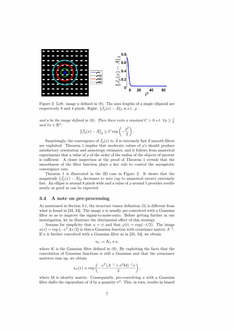
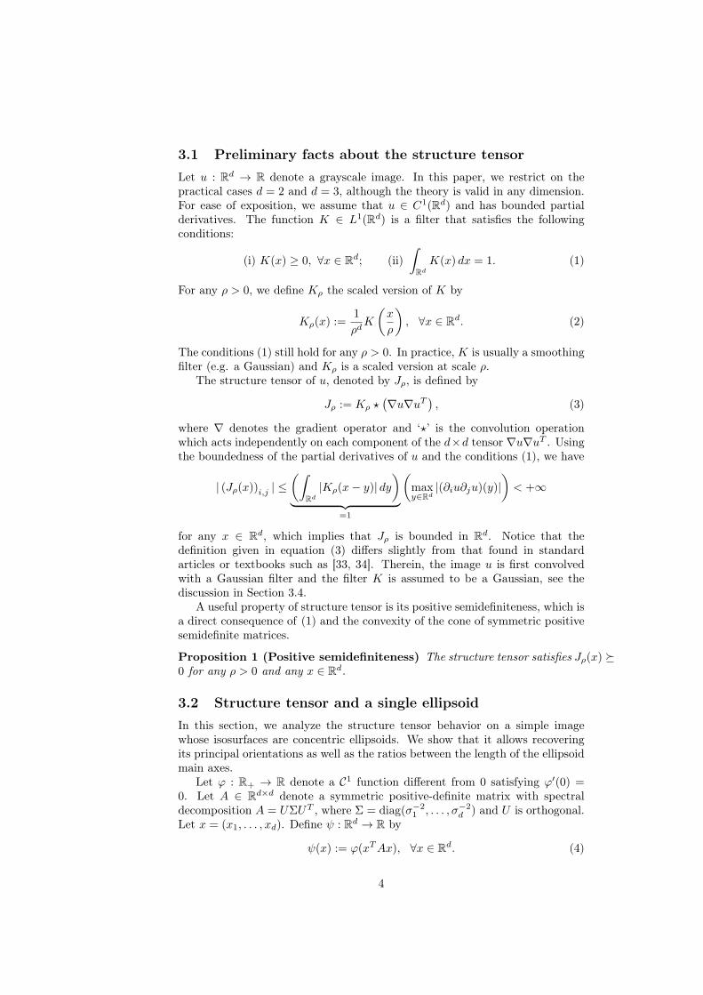
Figure 2: Left: image u defined in (8). The axes lengths of a single ellipsoid arerespectively 8 and 4 pixels. Right: ‖Jρ(x)− A‖2 w.r.t. ρ.

and u be the image defined in (8). Then there exits a constant C > 0 s.t. ∀ρ ≥ 12

and ∀x ∈ Rd:∥∥Jρ(x)− A

∥∥2≤ C exp

(−ρ2

2

).

Surprisingly, the convergence of Jρ(x) to A is extremely fast if smooth filtersare exploited. Theorem 1 implies that moderate values of ρ’s should producesatisfactory orientation and anisotropy estimates, and it follows from numericalexperiments that a value of ρ of the order of the radius of the objects of interestis sufficient. A closer inspection at the proof of Theorem 1 reveals that thesmoothness of the filter function plays a key role to control the asymptoticconvergence rate.

Theorem 1 is illustrated in the 2D case in Figure 2. It shows that themagnitude ‖Jρ(x) − A‖2 decreases to zero (up to numerical errors) extremelyfast. An ellipse is around 8 pixels wide and a value of ρ around 5 provides resultsnearly as good as can be expected.

3.4 A note on pre-processing

As mentioned in Section 3.1, the structure tensor definition (3) is different fromwhat is found in [33, 34]. The image u is usually pre-convolved with a Gaussianfilter so as to improve the signal-to-noise-ratio. Before getting further in ourinvestigation, let us illustrate the detrimental effect of this strategy.

Assume for simplicity that u = ψ and that ϕ(t) = exp(−t/2). The imageu(x) = exp

(−xTAx/2

)is thus a Gaussian function with covariance matrix A−1.

If u is further convolved with a Gaussian filter as in [33, 34], we obtain

uσ := Kσ ⋆ u,

where K is the Gaussian filter defined in (9). By exploiting the facts that theconvolution of Gaussian functions is still a Gaussian and that the covariancematrices sum up, we obtain

uσ(x) ∝ exp

(−xT (A−1 + σ2Id)−1x

2

),

where Id is identity matrix. Consequently, pre-convolving u with a Gaussianfilter shifts the eigenvalues of A by a quantity σ2. This, in turn, results in biased

7

anisotropy estimates. For instance, in the 2D case, the structure tensor basedanisotropy obtained using uσ is

(λ−1max(A) + σ2

λ−1min(A) + σ2

)1/2

,

which is different from the ground truth anisotropy(

λmin(A)λmax(A)

)1/2

.

The simple analysis above shows that in practice, more advanced imagedenoising techniques that keep isosurfaces unchanged should be preferred overa simple convolution with a Gaussian filter. A wide choice is now available suchas anisotropic diffusion, total variation denoising, frame based regularization ornon-local methods [31, 27, 29, 7, 8].

4 Numerical validation

In this section, we conduct some numerical experiments to evaluate the structuretensors performance on synthetic and real data. The main biological problemaddressed in our experiments is the analysis of geometrical configurations of nu-clei in multicellular tumor spheroids. There are at least two reasons making thisanalysis relevant. First, tumor development is associated with a disorganizationof the tissue. The role played by this disorganization is not well understood yetand it has been shown that it could have an impact on tumor cell behavior [36].Second, among the key parameters involved in tumor growth, those related tomechanical forces seem to play a critical role [21, 30, 9]. The elongation of nu-clei in a preferential direction is an indicator of local stresses [14, 32]. Assessingthe anisotropy and orientation of nuclei in their micro-environment is thereforecrucial to better understand tumor organization and mechanics.

4.1 Implementation details

Up to now, we only performed theoretical analyses in the continuous domain.In practice, the structure tensor should be adapted to the discrete setting.

The discrete gradient operator ∇ is defined by ∇ =

∂1...∂d

. In all reported

experiments, the partial differential operators ∂i are defined as convolutionswith discrete kernels. From an asymptotic point of view any kernel leading to aconsistent discretization should provide good results. However, the kernel designturns out to be crucial to provide good orientation and anisotropy estimates.Key properties of discrete kernels are [35]: i) rotation invariance, ensuring areliable orientation estimation, ii) separability, ensuring faster computations andiii) no shift, implying the use of centered finite differences. Following thesecriteria, the authors of [35] suggested to use the following filter in 2D:

h =1

32

−3 0 3−10 0 10−3 0 3

.

8

i.e. to set ∂1u = h ⋆ u and ∂2u = hT ⋆ u. Using the same methodology in 3D,one can derive the following filter (using Matlab notation):

h(:, :, 1) =

0.0153 0 −0.01530.0568 0 −0.05680.0153 0 −0.0153

,

h(:, :, 2) =

0.0568 0 −0.05680.2117 0 −0.21170.0568 0 −0.0568

and h(:, :, 3) = h(:, :, 1).

The gradient is computed in the space domain, while the convolution withKρ

is based on fast Fourier transforms. The overall computational complexity foran image with n pixels is therefore O(n log(n)). In practice, the structure tensorcan be computed in near real-time for 2D images and takes a few seconds for 3Dimages. It can be very easily parallelized on multicore or GPU architectures. Allcodes were written in Matlab 7.9 and experiments were conducted on a Lenovopersonal computer with Intel Core (TM) CPU 2.30GHZ and 8G memory.

4.2 2D and 3D synthetic data

In order to validate the theory, we first concentrate on 2D and 3D synthetictumor spheroids.

4.2.1 Synthesizing images

A tumor spheroid image u : Rd → R+ is synthesized by

u(x) =

N∑

i=1

ϕ((x− xci )

TAi(x− xci )), ∀x ∈ R

d, (10)

where N is the number of nuclei in the spheroid; ϕ is the bump function definedin (5); and xci ∈ Rd is the i-th nucleus center. The centers are drawn at randomin a d-dimensional sphere in such a way that the nuclei do not overlap.

• If d = 2, the matrix Ai ≻ 0 is defined by

Ai = Rθidiag(σ−21,i , σ

−22,i )(R

θi)T . (11)

where Rθi is the Givens transform (see Section 2); θi is the phase angle ofthe radial line issued from the origin and crossing the nucleus center xci ,see Fig. 1.

• If d = 3, the matrix Ai ≻ 0 is defined by

Ai = Rθi1,2R

γi

2,3diag(σ−21,i , σ

−22,i , σ

−23,i )(R

θi1,2R

γi

2,3)T , (12)

where θi, γi denote the compass and elevation angles of the radial linecrossing the ellipsoid center.

9

The anisotropy of the i-th nucleus is defined by

αi :=

mink=1,2,··· ,d

σk,i

maxk=1,2,··· ,d

σk,i. (13)

In our 2D experiment, the anisotropy αi increases linearly from the image centerto the outer layers of the sphere. For the 3D case, the anisotropy αi is set asconstant. Figure 3(a) and Figure 6 (a)-(b) display the 2D and 3D syntheticspheroids respectively.

4.2.2 Measuring the performance

In order to assess the structure tensor efficiency, we evaluate the following quan-tities:

• Orientation. Let vi denote the eigenvector corresponding to the largesteigenvalue of Jρ(x

ci ) and vi = (cos θi, sin θi) denote the ground truth ori-

entation. The following angles

∠(vi, vi), i = 1, 2, · · · , N, (14)

are used to evaluate the orientation accuracy in 2D. An angle close to0◦ indicates a good orientation estimation, while an angle close to 90◦ isthe worst possible estimate. For the 3D case, we choose for vi either thelargest eigenvector (prolate spheroid) ot the smallest eigenvector (oblatespheroid).

• Anisotropy. The structure tensor based anisotropy is defined by αi =(λmin(Jρ(x

ci ))

λmax(Jρ(xci))

)1/2

. The ratio

αi/αi, i = 1, 2, · · · , N, (15)

is used to quantify the estimated anisotropy accuracy, where αi is ground-truth anisotropy, see (13). A ratio close to 1 indicates that the anisotropyis correctly evaluated.

• Spectral norm. In the experiments based on synthetic images, a matrixA(x) can be associated to every point of the image domain. We cantherefore evaluate the spectral norm ‖Jρ(x)− A(x)‖2 everywhere and notonly at the nuclei centers.

4.2.3 2D synthetic data

We report numerical results on the 2D synthetic spheroid displayed in Figure3(a). The spheroid is first approximated by the nuclei convex hull, denotedby H. The green curve in Figure 3(d) represents the convex hull boundary1,denoted by ∂H. Note that the upcoming analyses are all restricted to the convexhull.

1In Matlab, this result can be obtained by first thresholding the image and then usingthe quickhull algorithm [2] (convhull command).

10

(a) (b) (c)

(d) (e) (f)

Figure 3: 2D synthetic data (a) 512×512 synthetic tumor spheroid (b) ground-truth orientations (c) ground-truth anisotropy (d) ground-truth orientations (e)Structure tensor based orientations (f) Structure tensor based anisotropy.

We use the value ρ = 5 in (3), this value is to be compared with the smallaxis of the ellipses that is σ1 = 10 and the large axis which ranges σ2 from10 to 32. An adequate value for ρ is of the order of the radius of the objectsof interest. Figure 3 (e)-(f) show the structure tensor based orientations andanisotropies which should be compared to the ground truth ones in Figure 3(b)-(c). The orientations and anisotropy are clearly very well estimated. Thisis somehow surprising since for this image, only a small number of cells sharethe same orientation and anisotropy locally. This favorable behavior is anotherillustration of the fast convergence speed obtained in Theorem 1.

To further quantify the accuracy of the results, the quantities (14)-(15) areevaluated. The histograms of both quantities are displayed in Figure 4. Theyshow that approximately 95% of estimated orientations have an angular errorbelow 4◦. Similarly, approximately 65% of estimated anisotropies have a anerror below 10%.

Finally, when using synthetic data, a ground-truth structure tensor A(x) canbe defined at every point of the image domain. We can thus compare the fourcoefficients of the 2 × 2 matrix A(x) with the coefficients of Jρ. The distance‖Jρ − A‖2 can also be evaluated at every point of the image domain, see Figure5. We observe that the structure tensor approximates accurately the groundtruth tensor.

4.2.4 3D synthetic data

We now test the structure tensor efficiency on 3D synthetic data generatedby formula (12), see Figures 6(a) for an oblate example and (b) for a prolateexample. The structure tensor Jρ is computed with ρ = 5. The estimatedorientations are displayed in Figure 6 (e) and (f) while the ground truth orien-

11

Figure 4: Analysis of structure tensor based accuracy for the 2D test case.Histograms of orientations errors (left) and of anisotropy errors (right).

Figure 5: Four coefficients of matrix A (left), four coefficients of matrix Jρ(center) and error map ‖Jρ − A‖2 (right).

tations are displayed in Figure 6 (c) and (d). The orientation is well retrieved.This is also confirmed by the histogram in Figure 7. Moreover, the histogramof anisotropy discrepancies show that approximately 70% of the anisotropiesare evaluated with an error below 10%. Overall, these results confirm that thestructure tensor is also very attractive to estimate anisotropies and orientationsfor 3D data.

4.3 Performance evaluation on real spheroid images

We now evaluate the structure tensor based orientation and anisotropy on a 2Dreal image. The image that we use in our experiment contains 1465 nuclei. The’gold standard’ reference was obtained manually. The scalar ρ is set to 10 inthis section. This value was selected manually and corresponds roughly to theradius of the nuclei.

The gold standard and estimated orientations are displayed in Figure 8.The orientation and anisotropy errors are presented in Figure 9(a) and (b)respectively.

Let us emphasize that the gold standard is subject to many errors sincei) a preferential orientation cannot be defined properly on isotropic cells andii) fitting a thousand ellipses manually is subject to many errors. Moreover,real data strongly depart from the ideal models considered in Section 3 since(i) the SNR of real tumor spheroid image is typically low due to noise, blur,variations in illumination, etc; (ii) the nuclei geometry is only approximatelyellipsoidal; (iii) the nuclei may overlap in 2D. Despite the rather poor quality of

12

(a) (c) (e)

(b) (d) (f)

Figure 6: 3D synthetic data (size: 128× 128× 128). (a) spheroid with σ1 : σ2 :σ3 = 5 : 5 : 2. (b) spheroid with σ1 : σ2 : σ3 = 5 : 2 : 2. (c)-(d) ground truthorientations of spheroids (a) and (b) respectively. (e)-(f) structure tensor basedorientations.

Figure 7: Analysis of structure tensor based errors for 3D synthetic data fromFigure 6. Histograms of orientations errors (left) and of anisotropy errors (right).

13

data and gold standard, the results fit remarkably well. Overall the orientationis evaluated with an error no larger 20◦ while the anisotropy seldom exceeds50% error. Finally, note that the preferential orientation is not well defined atthe image center since cells are near isotropic.

In Figure 9(c) we plot the median, mean and 25% ∼ 75% percentiles ofthe angle error (14) with respect to the distance to the spheroid boundary.The notation ‘dist(xci , ∂H)’ stands for the Euclidean distance from the nucleuscenter xci to the spheroid boundary. Figure 9(c) indicates that structure tensorprovides accurate orientations near the spheroid boundary and less accurate inthe center, since the median error increases from 7◦ close to the boundary to14◦ near the center.

4.4 Application to drug effects analysis on spheroids

As a proof of concept, spheroids were treated with latrunculin A, an inhibitorof actin polymerization. The comparison of (a) and (e) in Figure 10 showsthat this treatment induces a disorganization. We applied the structure tensorto extract the orientation and anisotropy maps in Figure 10 (c), (d), (g) and(h). The angle is measured with respect to the normal of the closest pointof the boundary. In other words, an angle equal to 90◦ means that the localorientation is parallel to the boundary, and an angle equal to 0◦ means that thelocal orientation is normal to the boundary.

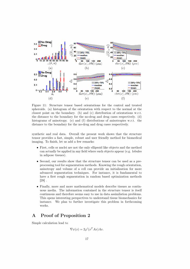
The results obtained show a decrease of both nuclei anisotropy and alignmentwith the spheroid boundary in the outer layers after treatment. This observationis confirmed by the graphs showed in Figure 11. In Figure 11(a) we compare thealignement of the nuclei with respect to the boundary with or without treatment.In Figures 11(b) and (c) we present the alignment with respect to the distanceto the boundary. We observe that the mean angle at the origin is around 80◦ forthe control spheroid and 60◦ for the treated spheroid, indicating that the drugtends to desalign the nuclei with respect to the spheroid boundary. Moreover,in Figure 11 (b), the gray zone is narrow at the origin, reflecting the fact thatnearly all nuclei near are well aligned with the boundary in the outer layers. Onthe contrary, the gray zone at the origin of the graph in Figure 11 (c) is thick,indicating that the orientation is much more erratic.

In Figure 11(d) we present the distribution of anisotropy for the control andthe treated spheroid. In Figures 11 (e) and (f) we present the anisotropy withrespect to the distance to the boundary. We observe that the mean anisotropynear the spheroid boundary is approximately equal to 0.6 for the control spheroidand 0.8 for the treated spheroid, indicating that nuclei are more round for thetreated case.

As a summary, our methodology allows quantifying both the change of align-ment and the decrease of anisotropy and could therefore have interesting appli-cations in high content throughput.

5 Outlook

We proposed an original theoretical analysis of structure tensors, justifying theiruse for evaluating orientations and anisotropies of cells or nuclei in 2D or 3Dimages. Our theoretical results were validated by numerical experiments, on

14

Figure 8: Comparison of ground truth orientations (top) and estimated orien-tations (bottom) on spheroid sections. Nuclei are stained using DAPI. Imageswere acquired using epifluorescence microscope (LEICA DM5000) and 10X ob-jective NA:0.3. Scale bar: 100µm.

(a) (b) (c)

Figure 9: Quantification of structure tensor based results for the 2D experimen-tal test case. (a) histogram of orientation error, (b) histogram of anisotropyerror, (c) structure tensor based orientations with respect to nuclei locations.

15

(a) (e)

(b) (f)

(c) (g)

(d) (h)

Figure 10: (a) and (e): Images of Tumor spheroids cryosections with nucleilabelled using DAPI. Images were obtained as in Figure 8. Top row: controlspheroid (with no drug). Bottom row: treated with latrunculin. (b) and (f):orientation map. (c) and (g): angle maps. An angle equal to 90◦ indicates thatnuclei are aligned with the spheroid boundary. (d) and (h) anisotropy map.Scale bar: 100µm.

16

(a) (b) (c)

(d) (e) (f)

Figure 11: Structure tensor based orientations for the control and treatedspheroids. (a) histogram of the orientation with respect to the normal at theclosest point on the boundary. (b) and (c) distribution of orientations w.r.t.the distance to the boundary for the no-drug and drug cases respectively. (d)histograms of anisotropy. (e) and (f) distributions of anisotropies w.r.t. thedistance to the boundary for the no-drug and drug cases respectively.

synthetic and real data. Overall the present work shows that the structuretensor provides a fast, simple, robust and user friendly method for biomedicalimaging. To finish, let us add a few remarks:

• First, cells or nuclei are not the only ellipsoid like objects and the methodcan actually be applied in any field where such objects appear (e.g. lobulesin adipose tissues).

• Second, our results show that the structure tensor can be used as a pre-processing tool for segmentation methods. Knowing the rough orientation,anisotropy and volume of a cell can provide an initialization for moreadvanced segmentation techniques. For instance, it is fundamental tohave a first rough segmentation in random based optimization methods[28] .

• Finally, more and more mathematical models describe tissues as contin-uous media. The information contained in the structure tensor is itselfcontinuous and therefore seems easy to use in data assimilation problems.This opens interesting perspectives to understand tissue biomechanics forinstance. We plan to further investigate this problem in forthcomingworks.

A Proof of Proposition 2

Simple calculation lead to

∇ψ(x) = 2ϕ′(xTAx)Ax.

17

Therefore

Jρ(0) =

∫

Rd

Kρ(−x)(∇ψ∇ψT )(x) dx

= 4A

(∫

Rd

(ϕ′(xTAx))2xxTKρ(x) dx

)AT .

But if ρ >√d/2 then Kρ is constant on the domain where ψ does not vanish.

Therefore by using the change of variable y = Σ1

2UTx, we obtain:

Jρ(0) ∝ |Σ− 1

2 |AUΣ− 1

2

(∫

Rd

ϕ′(‖y‖22)2yyT dy

)

︸ ︷︷ ︸∝Id

Σ− 1

2UTAT

∝ A.

Since Kρ is constant on a neighborhood of the domain where ψ does not vanish,Jρ is invariant by small translations hence Jρ is locally constant around 0.

B Proof of Proposition 3

We denote B(x0, ρ) = {x | ‖x − x0‖2 ≤ ρ} the Euclidian ball centered at x0with radius ρ and S(x0, ρ) = {x | ‖x− x0‖2 ≤ ρ} the Euclidian sphere centeredat x0 with radius ρ. We have

Jρ(x0) =1

ρd

∫

B(x0,ρ)

(∇u∇uT )(x) dx.

The image u is a sum of (non-overlapping) replicates of ψ. From Proposition 2,we know that all the replicates of ψ with support included in B(x0, ρ) will have acontribution to Jρ(x) proportional to A while the ones with support intersectingS(x0, ρ) have a contribution that can be considered as a bias, whose componentsare bounded by

∫Rd |∂iψ∂jψ|(x) dx. Let I = {i ∈ Zd | supp(ψ(·−i)) ⊂ B(x0, ρ)}

and J = {j ∈ Zd | supp(ψ(· − j)) ∩ S(x0, ρ) 6= ∅}. For sufficiently large ρ,|I| ∝ ρd (the volume of a ball of radius ρ) while |J | ∝ ρd−1 (the area of thesphere). Therefore

Jρ(x0) ∝ (ρdA+ ρd−1Bρ)/ρd,

where Bρ is some bias of bounded amplitude. This implies that

‖Jρ(x0)− A‖2 = O (1/ρ) .

C Proof of Theorem 1

The non-smoothed structure tensor is defined by

J0 = ∇u∇uT

= (X ⋆∇ψ) · (X ⋆∇ψ)T

= ((∂iψ∂jψ) ⋆X)i,j ,

18

where the last equality follows from the fact that the functions are nonover-lapping. By exploiting the facts that Jρ = Kρ ⋆ J0 and X = X, it comesthat

Jρ =((∂iψ∂jψ) · X · Kρ

)1≤i,j≤d

=

∑

k∈Zd

(∂iψ∂jψ)(k)Kρ(k)δk

1≤i,j≤d

.

This analysis provides a Fourier series decomposition of Jρ:

Jρ(x) =

∑

k∈Zd

(∂iψ∂jψ)(k)Kρ(k) exp(−2iπ〈x, k〉)

1≤i,j≤d

.

Moreover (1)-(ii) implies that Kρ(0) = 1, and for all i, j:∣∣∣(Jρ(x))i,j − (∂iψ∂jψ)(0)

∣∣∣

=

∣∣∣∣∣∣∑

k∈Zd\{0}

(∂iψ∂jψ)(k)Kρ(k) exp(−2iπ〈x, k〉)

∣∣∣∣∣∣

≤∑

k∈Zd\{0}

∣∣∣(∂iψ∂jψ)(k)∣∣∣∣∣∣Kρ(k)

∣∣∣

By denoting y = Σ1

2UTx, we obtain:(∂iψ∂jψ)(0)

)1≤i,j≤d

=

(∫

Rd

(∂iψ∂jψ)(x)

)

1≤i,j≤d

= 4A

(∫

Rd

ϕ′(xTAx)2xxT dx

)

1≤i,j≤d

AT

= 4|Σ− 1

2 |AUΣ− 1

2

(∫

Rd

ϕ′(‖y‖22)yyT dx

)

1≤i,j≤d︸ ︷︷ ︸∝Id

Σ− 1

2UTAT

∝ A.

Since ψ ∈ C1 with bounded support, c = ‖∂iψ∂jψ‖1 < +∞. Therefore

‖∂iψ∂jψ‖∞ ≤ c. Moreover, Kρ(k) = K(ρk) so that

∑

k∈Zd\{0}

∣∣∣(∂iψ∂jψ)(k)∣∣∣∣∣∣Kρ(k)|

∣∣∣ ≤ c∑

k∈Zd\{0}

|Kρ(k)|

= c∑

k∈Zd\{0}

|K(ρk)|

∝∑

k∈Zd\{0}

exp

(−ρ2‖k‖22

2

).

19

We now remark that

∑

k∈Zd

exp

(−ρ2‖k‖22

2

)=

∑

j∈Z

exp

(−ρ2j2

2

)

d

=

1 + 2

∑

j≥1

exp

(−ρ2j2

2

)

d

= (1 + 2u(ρ))d

= 1 + 2du(ρ) +Oρ→+∞(u(ρ))

where

u(ρ) =∑

j≥1

exp

(−ρ2j2

2

)≤

∑

j≥1

exp

(−ρ2j

2

)=

exp(−ρ2

2)

1− exp(−ρ2

2)

.

Since u(ρ) is asymptotic to exp(−ρ2

2) when ρ→ ∞ the claim is proved.

Acknowledgement

The authors would like to thank the TRI-Genotoul and ITAV-USR3505 imagefacilities and all the members of ITAV for providing a nice research environment.

Funding This work was supported by the ANR SPH-IM-3D (ANR-12-BSV5-0008), the NNSFC Grant 11301055 and la Fondation pour la Recherche Médicale(équipe labelisée 2012). A. D. is recipient of a doctoral fellowship from theAssociation pour la Recherche contre le Cancer and is as student of the écolede l’INSERM Liliane Bettencourt.

References

[1] D Ambrosi and F Mollica. On the mechanics of a growing tumor. Interna-tional Journal of Engineering Science, 40(12):1297–1316, 2002.

[2] C Bradford Barber, David P Dobkin, and Hannu Huhdanpaa. The quickhullalgorithm for convex hulls. ACM Transactions on Mathematical Software(TOMS), 22(4):469–483, 1996.

[3] Josef Bigun, Goesta H Granlund, and Johan Wiklund. Multidimensionalorientation estimation with applications to texture analysis and opticalflow. Pattern Analysis and Machine Intelligence, IEEE Transactions on,13(8):775–790, 1991.

[4] Isabelle Bonnet, Philippe Marcq, Floris Bosveld, Luc Fetler, Yohanns Bel-laïche, and François Graner. Mechanical state, material properties andcontinuous description of an epithelial tissue. Journal of The Royal SocietyInterface, page rsif20120263, 2012.

20

[5] Ronald N Bracewell. The fourier transform and its applications. McGraw-Hill, 1978.

[6] Didier Bresch, Thierry Colin, Emmanuel Grenier, Benjamin Ribba, OlivierSaut, et al. A viscoelastic model for avascular tumor growth. 2009.

[7] Antoni Buades, Bartomeu Coll, and J-M Morel. A non-local algorithmfor image denoising. In Computer Vision and Pattern Recognition, 2005.CVPR 2005. IEEE Computer Society Conference on, volume 2, pages 60–65. IEEE, 2005.

[8] Kostadin Dabov, Alessandro Foi, Vladimir Katkovnik, and Karen Egiazar-ian. Image denoising by sparse 3-d transform-domain collaborative filtering.Image Processing, IEEE Transactions on, 16(8):2080–2095, 2007.

[9] Annaïck Desmaison, Céline Frongia, Katia Grenier, Bernard Ducommun,and Valérie Lobjois. Mechanical stress impairs mitosis progression in multi-cellular tumor spheroids. PloS one, 8(12):e80447, 2013.

[10] Salvatore Federico and T Christian Gasser. Nonlinear elasticity of biolog-ical tissues with statistical fibre orientation. Journal of the Royal SocietyInterface, 7(47):955–966, 2010.

[11] Edouard Fonck, Georg G Feigl, Jean Fasel, Daniel Sage, Michael Unser,Daniel A Rüfenacht, and Nikolaos Stergiopulos. Effect of aging on elastinfunctionality in human cerebral arteries. Stroke, 40(7):2552–2556, 2009.

[12] Wolfgang Förstner and Eberhard Gülch. A fast operator for detectionand precise location of distinct points, corners and centres of circular fea-tures. In Proc. ISPRS intercommission conference on fast processing ofphotogrammetric data, pages 281–305, 1987.

[13] Gösta H Granlund and Hans Knutsson. Signal processing for computervision, volume 2. Springer, 1995.

[14] Farshid Guilak. Compression-induced changes in the shape and volume ofthe chondrocyte nucleus. Journal of biomechanics, 28(12):1529–1541, 1995.

[15] Chris Harris and Mike Stephens. A combined corner and edge detector. InAlvey vision conference, volume 15, page 50. Manchester, UK, 1988.

[16] JD Humphrey. Review paper: Continuum biomechanics of soft biologicaltissues. Proceedings of the Royal Society of London. Series A: Mathemati-cal, Physical and Engineering Sciences, 459(2029):3–46, 2003.

[17] JD Humphrey and KR Rajagopal. A constrained mixture model for growthand remodeling of soft tissues. Mathematical models and methods in appliedsciences, 12(03):407–430, 2002.

[18] Raphael Jorand, Gwénaële Le Corre, Jordi Andilla, Amina Maandhui, Cé-line Frongia, Valérie Lobjois, Bernard Ducommun, and Corinne Lorenzo.Deep and clear optical imaging of thick inhomogeneous samples. PloS one,7(4):e35795, 2012.

21

[19] Bruce D Lucas and Takeo Kanade. An iterative image registration tech-nique with an application to stereo vision. In IJCAI, volume 81, pages674–679, 1981.

[20] Andreas Menzel, Magnus Harrysson, and Matti Ristinmaa. Towards anorientation-distribution-based multi-scale approach for remodelling biolog-ical tissues. Computer methods in biomechanics and biomedical engineering,11(5):505–524, 2008.

[21] Fabien Montel, Morgan Delarue, Jens Elgeti, Laurent Malaquin, MarkusBasan, Thomas Risler, Bernard Cabane, Danijela Vignjevic, Jacques Prost,Giovanni Cappello, et al. Stress clamp experiments on multicellular tumorspheroids. Physical review letters, 107(18):188102, 2011.

[22] Nicolas Olivier, Miguel A Luengo-Oroz, Louise Duloquin, Emmanuel Faure,Thierry Savy, Israël Veilleux, Xavier Solinas, Delphine Débarre, PaulBourgine, Andrés Santos, et al. Cell lineage reconstruction of early zebrafishembryos using label-free nonlinear microscopy. Science, 329(5994):967–971,2010.

[23] Kannappan Palaniappan, Ilker Ersoy, and Sumit K Nath. Moving objectsegmentation using the flux tensor for biological video microscopy. In Ad-vances in Multimedia Information Processing–PCM 2007, pages 483–493.Springer, 2007.

[24] Sorin Pop, Alexandre C Dufour, Jean-François Le Garrec, Chiara V Ragni,Clémire Cimper, Sigolène M Meilhac, and Jean-Christophe Olivo-Marin.Extracting 3d cell parameters from dense tissue environments: applicationto the development of the mouse heart. Bioinformatics, 29(6):772–779,2013.

[25] A Ravishankar Rao and Brian G. Schinck. Computing oriented texturefields. CVGIP: Graphical Models and Image Processing, 53(2):157–185,1991.

[26] Rana Rezakhaniha, Aristotelis Agianniotis, Jelle Tymen ChristiaanSchrauwen, Alessandra Griffa, Daniel Sage, CVC Bouten, FN Van de Vosse,Michaël Unser, and Nikolaos Stergiopulos. Experimental investigation ofcollagen waviness and orientation in the arterial adventitia using confocallaser scanning microscopy. Biomechanics and modeling in mechanobiology,11(3-4):461–473, 2012.

[27] Leonid I Rudin, Stanley Osher, and Emad Fatemi. Nonlinear total vari-ation based noise removal algorithms. Physica D: Nonlinear Phenomena,60(1):259–268, 1992.

[28] Emmanuel Soubies, Pierre Weiss, and Xavier Descombes. A 3d segmenta-tion algorithm for ellipsoidal shapes. application to nuclei extraction. InProceedings ICPRAM, 2013.

[29] J-L Starck, Emmanuel J Candès, and David L Donoho. The curvelettransform for image denoising. Image Processing, IEEE Transactions on,11(6):670–684, 2002.

22

[30] Triantafyllos Stylianopoulos, John D Martin, Vikash P Chauhan, Sa-loni R Jain, Benjamin Diop-Frimpong, Nabeel Bardeesy, Barbara L Smith,Cristina R Ferrone, Francis J Hornicek, Yves Boucher, et al. Causes, conse-quences, and remedies for growth-induced solid stress in murine and humantumors. Proceedings of the National Academy of Sciences, 109(38):15101–15108, 2012.

[31] David Tschumperlé. Fast anisotropic smoothing of multi-valued images us-ing curvature-preserving pde’s. International Journal of Computer Vision,68(1):65–82, 2006.

[32] Marie Versaevel, Thomas Grevesse, and Sylvain Gabriele. Spatial coordi-nation between cell and nuclear shape within micropatterned endothelialcells. Nature communications, 3:671, 2012.

[33] Joachim Weickert. Anisotropic diffusion in image processing, volume 1.Teubner Stuttgart, 1998.

[34] Joachim Weickert. Coherence-enhancing diffusion filtering. InternationalJournal of Computer Vision, 31(2-3):111–127, 1999.

[35] Joachim Weickert and Hanno Scharr. A scheme for coherence-enhancingdiffusion filtering with optimized rotation invariance. Journal of VisualCommunication and Image Representation, 13(1):103–118, 2002.

[36] Britta Weigelt and Mina J Bissell. Unraveling the microenvironmentalinfluences on the normal mammary gland and breast cancer. In Seminarsin cancer biology, volume 18, pages 311–321. Elsevier, 2008.

23