University of Warsaw

Faculty of Mathematics, Informatics and Mechanics

Aleksandra Paluszy«ska

Student no. 320255

Structure mining and knowledge

extraction from random forest with

applications to The Cancer Genome

Atlas project

Master's thesis

in MATHEMATICSin the eld of APPLIED MATHEMATICS

Supervisor:

dr hab. Przemysªaw BiecekInstytut Matematyki Stosowanej i Mechaniki

July 2017

Supervisor's statement

Hereby I conrm that the presented thesis was prepared under my supervision and

that it fulls the requirements for the degree of Master of Mathematics.

Date Supervisor's signature

Author's statement

Hereby I declare that the presented thesis was prepared by me and none of its contents

was obtained by means that are against the law.

The thesis has never before been a subject of any procedure of obtaining an academic

degree.

Moreover, I declare that the present version of the thesis is identical to the attached

electronic version.

Date Author's signature

Abstract

The thesis discusses various approaches to interpreting black boxes, i.e. predictive modelswith extremely complicated structure. In particular, I consider random forests that oftenproduce accurate predictions, which are not easily explained in terms of relative importanceof input variables.

As information on how the explanatory variables inuence prediction is often critical inapplications, I introduce a new R package, randomForestExplainer, that calculates new andexisting measures of variable importance in random forests. More importantly, the packageproposes new ways of visualizing relative importance of variables and provides a wrap-upfunction that summarizes a given random forest in various ways.

Finally, I demonstrate the usage of the package in an analysis of the Cancer Genome Atlasdata concerning glioblastoma cancer. My data set has many more variables than observations,which leads to shallow trees in the forest and makes the assessment of variable importanceparticularly hard. Thus, using this example I show how the package works in such problematicsettings.

Keywords

random forests, structure mining, visualization, variable importance, feature importance

Thesis domain (Socrates-Erasmus subject area codes)

11.2 Statistics11.3 Informatics, Computer Science

Subject classication

68 Computer Science68Q Theory of Computing68Q32 Computational learning theory62 Statistics62P Applications62P10 Applications to biology and medical sciences

Tytuª pracy w jezyku polskim

Analiza struktury i ekstrakcja wiedzy z lasów losowych z przyk³adami zastosowañ dladanych The Cancer Genome Atlas

Contents

Contents . . . . . . . . . . . . . . . . . . . . . . . . . . . . . . . . . . . . . . . . . . . 3

Introduction . . . . . . . . . . . . . . . . . . . . . . . . . . . . . . . . . . . . . . . . 5

1. Structure mining of predictive models . . . . . . . . . . . . . . . . . . . . . . 71.1. Predictive models . . . . . . . . . . . . . . . . . . . . . . . . . . . . . . . . . . 7

1.1.1. The problem . . . . . . . . . . . . . . . . . . . . . . . . . . . . . . . . 71.1.2. Data models . . . . . . . . . . . . . . . . . . . . . . . . . . . . . . . . 71.1.3. Algorithmic models . . . . . . . . . . . . . . . . . . . . . . . . . . . . . 8

1.2. Structure mining . . . . . . . . . . . . . . . . . . . . . . . . . . . . . . . . . . 91.2.1. Local Interpretable Model-agnostic Explanations . . . . . . . . . . . . 91.2.2. Visualization of the model . . . . . . . . . . . . . . . . . . . . . . . . . 10

1.3. Random forests . . . . . . . . . . . . . . . . . . . . . . . . . . . . . . . . . . . 121.3.1. Construction of a random forest . . . . . . . . . . . . . . . . . . . . . . 131.3.2. Analysis using random forests . . . . . . . . . . . . . . . . . . . . . . . 171.3.3. Importance of variables in a forest . . . . . . . . . . . . . . . . . . . . 18

2. Functionality of the R package randomForestExplainer . . . . . . . . . . . . 232.1. Minimal depth distribution . . . . . . . . . . . . . . . . . . . . . . . . . . . . 24

2.1.1. Calculate the distribution . . . . . . . . . . . . . . . . . . . . . . . . . 242.1.2. Mean minimal depth . . . . . . . . . . . . . . . . . . . . . . . . . . . . 252.1.3. Plot the distribution . . . . . . . . . . . . . . . . . . . . . . . . . . . . 27

2.2. Variable importance . . . . . . . . . . . . . . . . . . . . . . . . . . . . . . . . 292.3. Interactions of variables . . . . . . . . . . . . . . . . . . . . . . . . . . . . . . 33

2.3.1. Conditional minimal depth . . . . . . . . . . . . . . . . . . . . . . . . 342.3.2. Prediction on a grid . . . . . . . . . . . . . . . . . . . . . . . . . . . . 37

2.4. Explain the forest . . . . . . . . . . . . . . . . . . . . . . . . . . . . . . . . . . 38

3. Application to The Cancer Genome Atlas data . . . . . . . . . . . . . . . . 413.1. The data and random forest . . . . . . . . . . . . . . . . . . . . . . . . . . . . 413.2. Distribution of minimal depth . . . . . . . . . . . . . . . . . . . . . . . . . . . 423.3. Various variable importance measures . . . . . . . . . . . . . . . . . . . . . . 443.4. Variable interactions . . . . . . . . . . . . . . . . . . . . . . . . . . . . . . . . 473.5. Explain the forest . . . . . . . . . . . . . . . . . . . . . . . . . . . . . . . . . . 50

Summary . . . . . . . . . . . . . . . . . . . . . . . . . . . . . . . . . . . . . . . . . . 53

Appendices . . . . . . . . . . . . . . . . . . . . . . . . . . . . . . . . . . . . . . . . . 55

3

A. List of functions available in randomForestExplainer . . . . . . . . . . . . . . 55

B. Additional examples . . . . . . . . . . . . . . . . . . . . . . . . . . . . . . . . . 57B.1. Multi-label classication: breast cancer data . . . . . . . . . . . . . . . . . . . 57B.2. Regression: PISA data . . . . . . . . . . . . . . . . . . . . . . . . . . . . . . . 57

List of Figures . . . . . . . . . . . . . . . . . . . . . . . . . . . . . . . . . . . . . . . 69

List of Algorithms . . . . . . . . . . . . . . . . . . . . . . . . . . . . . . . . . . . . . 71

Bibliography . . . . . . . . . . . . . . . . . . . . . . . . . . . . . . . . . . . . . . . . 73

4

Introduction

In recent years the use of predictive models, which predict an outcome using a set of inputs,has become more widespread than ever. Abundance of data and ample computing powercreate opportunities for the emergence of new elds that rely on predictive modelling, suchas speech or image recognition, which are inherently dierent from the established ones andmay require dierent kinds of models. Traditionally the focus of statistical modelling was tounderstand the data-generating process so predictive ability of the model was a sort of usefulbyproduct of the analysis.

Nowadays, many applications primarily call for accurate predictions due to the following:rst, nancial rewards may be driven by prediction accuracy (e.g., accurate facial recognitionboosts productivity of a security rm) and second, the nature of the data-generating processmay be too complex or not interesting enough to be analyzed as such (e.g., how the structureof pixels in an image shapes the probability of a face appearing in it).

Whenever a statistical model is used for prediction, a dierent sort of model assessmentis necessary than when building it in order to explain some natural phenomenon. Similarly,whenever a model built for the sole purpose of prediction is to be used in the decision-makingprocess, there is a pressing need of explaining how the prediction is made so that it can betrusted. If the model in question is a black box, i.e. it is so complex that there is no naturalway of interpreting it, an explanation has to be provided by what we call structure miningand knowledge extraction.

In this thesis I focus on random forests, one class of predictive black boxes that is recog-nized as capable of accurate prediction using relatively little computing power in comparisonto other methods (e.g., gradient boosting [5]). As a committee of decision trees, each built ona bootstrap sample of the data, random forests do not provide any natural way of measur-ing which variables drive the prediction. To address this issue I introduce a new R packagerandomForestExplainer that aims at explaining a forest in terms of distinguishing the vari-ables that are essential to its performance.

The package provides a few functions that calculate a set of measures of variable impor-tance including the ones already in use and some new ones such as the number of timesa predictor was used to split the root node of a tree in the forest. Most importantly,randomForestExplainer oers a wide variety of possibilities for visualizing the forest thathelp to understand its structure and assess importance of variables. Finally, it includes awrapper function that utilizes all capabilities of the package for a given random forest andproduces a HTML report summarizing the results. This allows the user to familiarize herselfwith the explanatory insight that the package oers for her forest without getting to knowthe details about how to produce each plot or data frame.

I demonstrate the capabilities of randomForestExplainer for a forest predicting whethera patient survives a year from diagnosis of glioblastoma cancer. The data come from TheCancer Genome Atlas Project [18] and contain 16117 predictors for 125 observations such ahigh number of variables relative to observations leads to shallow trees in the forest and this

5

in turn makes the assessment of variable importance particularly hard. As such problems arerecently ever more common in practice, the point of using this data set is to show how thenew package manages them.

The thesis is structured as follows: in Chapter 1 I discuss predictive models in general,present general methods of structure mining, formally dene random forests and existingmethods of measuring variable importance in them. Then, in Chapter 2 I present how eachrandomForestExplainer function works, what are its parameters and how it should be used.Finally, Chapter 3 contains a step-by-step application of the new package to the glioblastomadata set.

6

Chapter 1

Structure mining of predictive models

1.1. Predictive models

In this section we rst dene our problem as either a regression or classication task andintroduce its mathematical structure. Then, we present two main approaches to solvingthe problem: through a data model that requires certain assumptions concerning the data-generating process or with an algorithmic model that treats this process as a black box.

1.1.1. The problem

Lets assume that we observe pairs (y,x), where y will be called the response variable and xis a vector of length p of predictors. Moreover, we assume that y is a realization of randomvariable Y , while x is a realization of random variable X. We face the following problem:given observed inputs x we want to predict the expected value of Y . Usually, we assume thatY depends on X and the expected value of Y can be expressed as follows:

E(Y |X = x) = f(x), (1.1)

where f is a function f : Rp → Y that we call a predictive model. Moreover, if Y = R(i.e., the response is measured on a quantitative scale and is thus called quantitative) we callf a regression model and if Y = G1, G2, . . . , GK is a set of K possible groups to whichthe observation belongs, we use the term classication model. Fortunately, in our case thisdistinction will not matter much, as the models we discuss work equally well under bothsettings.

Throughout the paper we assume that we observe an n-element training sample

Z = (x1, y1), (x2, y2), . . . , (xn, yn). (1.2)

Using this knowledge we want to predict y for a given vector of values x; we denote theprediction as y(x). For simplicity, we will use the shorter notation y.

1.1.2. Data models

Until recently the main approach to predicting y from a set of inputs was to assume anunderlying data model. Breiman [3] refers to this as the data modelling culture in which oneassumes that the data are independently drawn from some distribution whose expectationcan be denoted as

E(Y |X = x) = f(x,βββ), (1.3)

7

where f is a known function and βββ is the vector of unknown parameters. Under such assump-tions one can estimate the unknown parameters using the available data.

In [15] Schmueli refers to this approach as explanatory modelling as it is often used fortesting the validity of causal theoretical models in which the variables in X cause the eectmeasured by Y . It is worth noting that this is most appropriate in settings where the un-derlying theory is important, sometimes to such an extent that it is given as a justicationfor the causal interpretation of the model. Furthermore, as Schmueli points out, this focuson theory is usually present at all stages of explanatory modelling including the choice ofindependent variables, model selection and validation. This leads to the conclusion that datamodels are indeed most useful when explaining a phenomenon is the focus and not necessarilywhen the sole purpose of modelling is prediction (this point is often made in the literature,most notably by Breiman [3]). More importantly, if the assumed model is not an accurateapproximation of the natural processes it may lead to wrong conclusions.

To give an example, generalized linear models are a class of widely-used data models thatcan be represented by the following equation:

E(Y |X = x) = g−1(xβββ), (1.4)

where g is usually referred to as the link function. The simplest examples of link functionsare: the identity function for linear regression, the logistic function for logistic regressionand the natural logarithm for Poisson regression. Regardless of the link function chosen, theparameters βββ = (β0, β1, . . . , βp)

T , of which the rst one is a constant and the others correspondto p independent variables, can be directly interpreted as measures of relative importance ofthose variables in the Y -generating stochastic process. Moreover, using classical statistics wecan test various hypotheses concerning these parameters (e.g., whether the true parameteris dierent than zero) and with some additional assumptions we can interpret the estimatedrelationship as causal.

1.1.3. Algorithmic models

In contrast to the data modelling culture, the algorithmic modelling culture (as called byBreiman in [3]) focuses on predictive accuracy of models. Although it also takes input variablesX and tries to nd a function f(X) that best predicts Y it rejects the idea that we canrestrict the search to some class of functions as in (1.4). The core assumption here is thatthe data-generating process is complex and unknown so, instead of approximating it, we usean algorithm that based on available data imitates natural outcomes most accurately. Theresulting model is usually not interpretable due to a very complicated structure and is thuscalled a black box.

The focus of algorithmic models on prediction makes them a valuable tool whenever themechanism of the data-generating process is not of main interest or there is no theory sup-porting an explanatory model. The rst scenario often appears in the industry, wheneverdecisions rely on accurate predictions of the future (e.g., weather forecast) and not on under-standing what drives them. The latter scenario is ever more common in emerging elds suchas speech, image and handwriting recognition [3]. In general, algorithmic models oer greaterpredictive accuracy than simple explanatory models as they are designed for the sole purposeof prediction.

Algorithmic models also oer a solution to two major problems with data models: themultiplicity of good models and the curse of dimensionality [3]. The rst of them concerns thefact that even a slight perturbation of the data or an alteration of the set of models considered(e.g., with or without some variable) may lead to major changes in the nal model, regardless

8

of whether it is a data or an algorithmic one. One solution is to average over a set ofcompeting models in order to stabilize the result this is often introduced as an inherent partof the model-building process of algorithmic models and is usually a minor complication ofan inherently complex black box1.

Finally, data models cannot usually include too many explanatory variables (e.g., nomore than the number of data points in the case of linear regression), so the dimensionof the analyzed data set often has to be reduced prior to modelling, which leads to loss ofinformation. Conversely, in algorithmic modelling it is usually the case that only computationpower limits the numer of input variables and nowadays this is not too big of a restriction.Clearly, this not only improves the aforementioned predictive accuracy but also eliminatesthe problem of variable selection as all variables and even many of their transformations canbe included in the black box. Breiman [3] calls this the blessing of dimensionality in contrastto the curse of dimensionality inherent to explanatory modelling. As in this paper our mainfocus is prediction accuracy and our motivating example is the high-dimensional problem ofpredicting whether a patient will die of cancer from The Cancer Genome Project data, fromnow on we will only consider algorithmic models.

1.2. Structure mining

We already discussed the fact that having a black box tuned to our problem (of either theregression or classication type) gives us a good chance of predicting the desired outcomevariable accurately. However, we cannot justify the prediction in any way, e.g. we have noway of knowing which input variables drive it, as our model has an inherently complicated,uninterpretable structure. This may be a big problem in applications, where such predictionsmust be at least partially explained to the decision-makers so they will trust them and, as aresult, use them.

To address this issue, we need to analyze the structure of our black box and in this sectionwe present some existing methods of doing this. We call it structure mining as it aims atdiscovering patterns and extracting knowledge from the vast and complex structure of theblack box. Sánchez, Rocktäschel, Riedel and Singh in [14] list three main approaches tothis: pedagogical, which analyzes the behavior of the model, decompositional, which aims atdividing the model into simpler parts to inspect each of them in turn and eclectic a mix ofthe two. In this section we focus on pedagogical methods, as they usually do not require anyadditional assumptions about the black box and we would like to start our discussion of blackboxes from a general perspective.

1.2.1. Local Interpretable Model-agnostic Explanations

The paper [13] by Riberio, Singh and Guerstin introduces a technique called Local InterpretableModel-agnostic Explanations (LIME). Its main idea is to approximate the black box f(x) byan interpretable model ξ(x) in the small neighborhood of the actual prediction, as measuredby πx(z) the structure of the black box is not explicitly considered. We present the methodfollowing [13] with slight modications due to notation dierences.

Let us dene πx(z) as the proximity measure between the input values for our observationx and z, which denes locality around x. Also, let ξ : Rp → Y be a model such that ξ ∈ H

1It is worth noting that this can also be done in the case of data models, but usually complicates theinterpretation. Also, data models are generally sensitive to inclusion/exclusion of some explanatory variablesand there is no simple way in determining a set of models (dierent in this respect) over which to average.

9

where H is a class of potentially interpretable models in contrast to our uninterpretable blackbox f . We denote the measure of complexity of ξ as Ω(ξ) if it is too high, ξ may be hard tointerpret (e.g., linear regression with too many parameters). Finally, let L(f, ξ, πx) measurehow unfaithfully ξ approximates f locally, as dened by πx.

LIME aims at producing an explanation ξ(x) of the black box f , which is both interpretableby humans (i.e., Ω(ξ) is suciently low) and locally faithful (i.e., gives similar results as theblack box in the vicinity of a given observation). This is obtained by the following:

ξ(x, f) = arg minh∈H

L(f, h, πx) + Ω(h). (1.5)

Note that this gives many possibilities of proceeding, depending on what class of interpretablemodels we consider, etc. As in [13] we focus on sparse linear models and use perturbation ofinputs to search for them.

In order to learn the behavior of our black box under varying inputs we approximateL(f, ξ, πx) by optimizing it on a perturbed sample drawn from the neighbourhood of x.In [13] the authors propose the following procedure: draw the number of elements of theperturbed sample K with equal probabilities from the set 1, 2, . . . , n. Then, uniformly drawK elements of our sample x1,x2, . . . ,xn to form the perturbed sample z1, z2, . . . , zK, sofor all i ∈ 1, 2, . . . ,K there exists a j ∈ 1, 2, . . . , n such that zi = xj . After repeating thisprocedure r times we obtain a set of perturbed samples Z so we can optimize the equation(1.5) over this set to get ξ(x).

For example, we might dene H as linear models, i.e. ξ(z) = zTβββ, and use locally weightedsquare loss function to measure the accuracy of approximation:

L(f, zTβββ, πx) =∑z∈Z

πx(z)[f(z)− zTβββ]2, πx(z) = exp

−dist(x, z)2

σ2

, (1.6)

where πx is the exponential kernel with width σ, dened on some distance function dist(). Toensure that the explanation is interpretable we may restrict the number of non-zero entries ofβββ to M , i.e. set Ω(ξ) = ‖βββ‖0 and add an additional restriction that Ω(ξ) ≤M .

1.2.2. Visualization of the model

Wickham, Cook and Hofman recognize visualization as a powerful tool for explaining statis-tical models and propose three main strategies of doing so (see [19]): visualizing the modelin the data space, analyzing a collection of models instead of a single one and exploring themodel-tting process. It is worth noting that, apart from approaching the issue of structuremining without any assumptions concerning the model as was the case for LIME, Wick-ham, Cook and Hofman focus on visual presentation of the model, to make it appealing to abroader audience and enhance its understanding. We summarize their main points in [19] byaddressing each of the aforementioned strategies in turn.

When using visual model descriptions we usually want to explain either what the modellooks like or how well it ts the data. In the rst case we consider changes to the modelcaused by those of its parameters or changes to parameters caused by those in the data.When it comes to exploring model tness, we can compare the shapes of the model and data,identify the regions of good or bad t and ones in which it can be improved. All this leads toour better understanding of the underlying process and improves out ability to meaningfullycriticize the model.

10

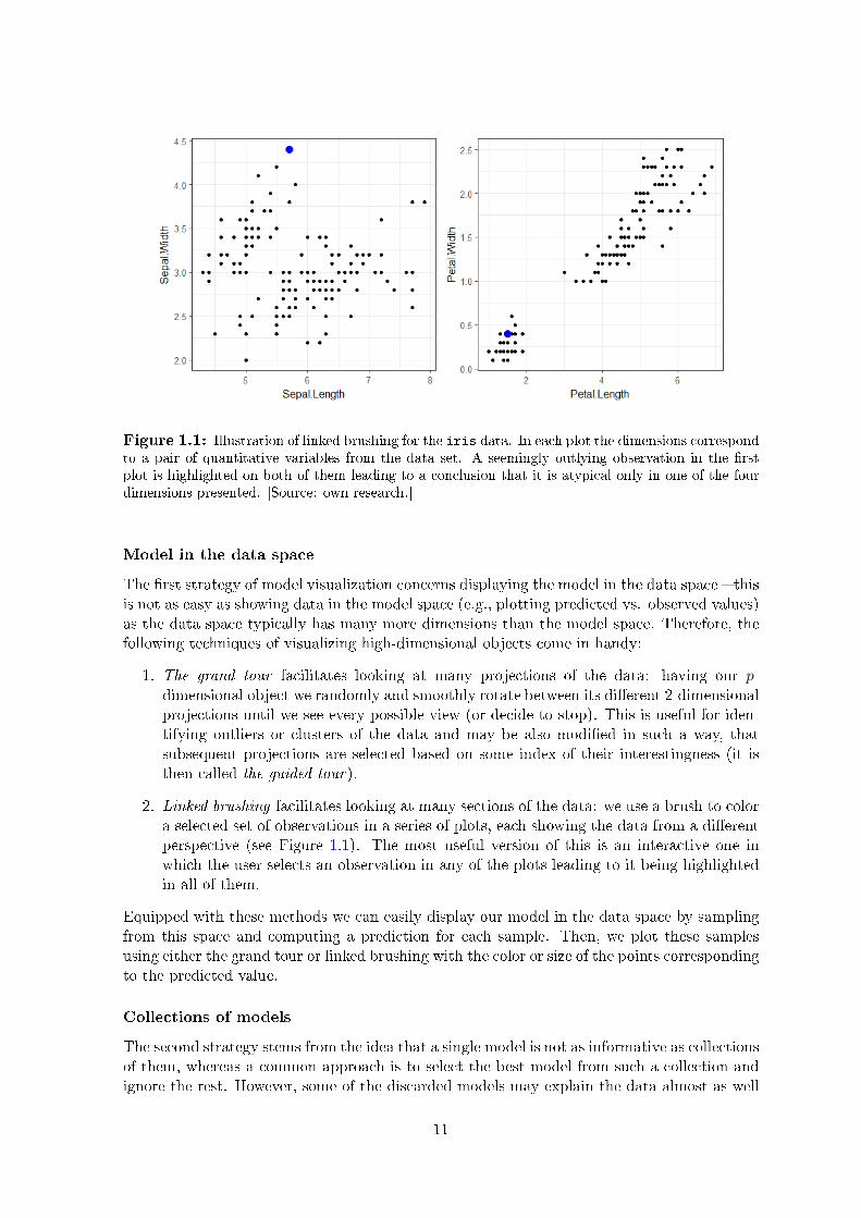
Figure 1.1: Illustration of linked brushing for the iris data. In each plot the dimensions correspondto a pair of quantitative variables from the data set. A seemingly outlying observation in the rstplot is highlighted on both of them leading to a conclusion that it is atypical only in one of the fourdimensions presented. [Source: own research.]

Model in the data space

The rst strategy of model visualization concerns displaying the model in the data space thisis not as easy as showing data in the model space (e.g., plotting predicted vs. observed values)as the data space typically has many more dimensions than the model space. Therefore, thefollowing techniques of visualizing high-dimensional objects come in handy:

1. The grand tour facilitates looking at many projections of the data: having our p-dimensional object we randomly and smoothly rotate between its dierent 2-dimensionalprojections until we see every possible view (or decide to stop). This is useful for iden-tifying outliers or clusters of the data and may be also modied in such a way, thatsubsequent projections are selected based on some index of their interestingness (it isthen called the guided tour).

2. Linked brushing facilitates looking at many sections of the data: we use a brush to colora selected set of observations in a series of plots, each showing the data from a dierentperspective (see Figure 1.1). The most useful version of this is an interactive one inwhich the user selects an observation in any of the plots leading to it being highlightedin all of them.

Equipped with these methods we can easily display our model in the data space by samplingfrom this space and computing a prediction for each sample. Then, we plot these samplesusing either the grand tour or linked brushing with the color or size of the points correspondingto the predicted value.

Collections of models

The second strategy stems from the idea that a single model is not as informative as collectionsof them, whereas a common approach is to select the best model from such a collection andignore the rest. However, some of the discarded models may explain the data almost as well

11

as the best one but lead to substantially dierent interpretations, presumably valuable whenwe try to understand the underlying process. To take this into account, one should visualizethe entire collection of models.

Unfortunately, we are usually able to visualize only a few models from the collection intheir entirety, so it is essential to somehow summarize them this is most easily done withdescriptive statistics that report model quality. Usually, these are specic to the class of mod-els considered (e.g., R2, information criteria or degrees of freedom for regression models), butthere are more universal ones like various summaries of residuals or, in the case of parameterestimation, statistics describing the distribution of estimates across models. In any case, ifwe have l models, n observations and p variables, we can think of descriptive statistics on vedierent levels [19]:

• model level: l observations, each corresponding to one model, e.g. prediction accuracy,

• model-estimate level: l × p observations, e.g. coecient estimates,

• estimate level: p observations, e.g. summary of estimates across models,

• model-observation level: l × n observations, e.g. inuence measures,

• observation level: n observations, e.g. average of residuals across models.

Having calculated descriptive statistics, we can use linked brushing for visualization in orderto connect statistics from dierent levels across plots.

The model-tting process

Finally, the third visualization strategy aims at exploring the model-tting process wheneverpossible, instead of only looking at the nal result. Wickham, Cook and Hofman note that thismay be particularly valuable if the algorithm used for model-tting is iterative, because thenwe observe how the consecutive versions of the model improve using their natural ordering.When it comes to visualization we can think of two main approaches exploiting this ordering:time series plots (i.e., time on the x-axis and a summary statistic on the y-axis) or moviesdepicting the evolution of the model (i.e., many static plots capturing dierent iterations ofthe model stringed together). Moreover, we could t the model multiple times using dierentstarting points for the algorithm to explore optima reached, as many algorithms only guaranteeconvergence to a local optimum (see Figure 1.2).

In summary, visualization is an important tool not only in data exploration but also inthe process of building statistical models. Therefore, in this paper we aim at explaining blackboxes with a strong emphasis on visualization.

1.3. Random forests

In this section we focus our attention on one class of predictive black boxes: random forests.We start by presenting their construction and motivation behind it to then discuss theirproperties in more detail. Finally, we address the issue of structure mining in this contextby presenting various measures of importance of explanatory variables included in the model.Throughout the section we rely heavily on the work of Hastie, Tibshirani and Friedman [5]and occasionally refer to the original work of Breiman [2] that laid the foundations of randomforests.

12

Figure 1.2: The model-tting process of simulated annealing with 20 random starts. The qualityof the model in any particular time is measured by a clumpiness index that is high when a divisionof the data into distinct groups emerges. Red points indicate four highest values. [Source: Wickham,Cook and Hofman [19], Figure 14.]

1.3.1. Construction of a random forest

Random forest is a collection of trees, each built on a dierent bootstrap sample of the data,from which an aggregate prediction is calculated [2]. This denition makes it natural to presentthe construction of a random forest by rst discussing its individual elements, decision trees,and then considering their whole collection.

Decision trees

First, we need to introduce terminology connected to decision trees. In mathematics a tree isdened as an undirected, acyclic and connected graph or, equivalently, an undirected graphin which any two vertices are connected by exactly one path [10]. In the context of trees thevertices are called nodes and edges branches. When it comes to decision trees it is convenientto use directed trees so that they can be depicted in such a way that on top we have a uniquestarting node, referred to as the root, which has only outgoing branches so that consecutivebranches and nodes are below it. If a branch starts at a node the latter is called a parent

and the node to which the branch points is called a daughter. Nodes without daughters arereferred to as leaves.

A decision tree is a model that partitions the p-dimensional space generated by predictorsinto L hypercubes Rl for l = 1, 2, . . . , L called decision regions and ts a simple model of Y(such as a constant) on each of them separately. Thus, the model has the following form2:

f(x) =

L∑l=1

cl1(x ∈ Rl), (1.7)

where cl is some constant,⋃L

l=1Rl = Rp and Rl ∩ Rk = ∅ for all l 6= k. This model can be

2For a multi-class classication problem the notation is slightly dierent instead of E(Y |X) = f(X) wewrite E(Y = k|X) = fk(X) for k = 1, 2, . . . ,K corresponding to the K possible values of Y so in (1.7) theconstant is indexed over both l and k.

13

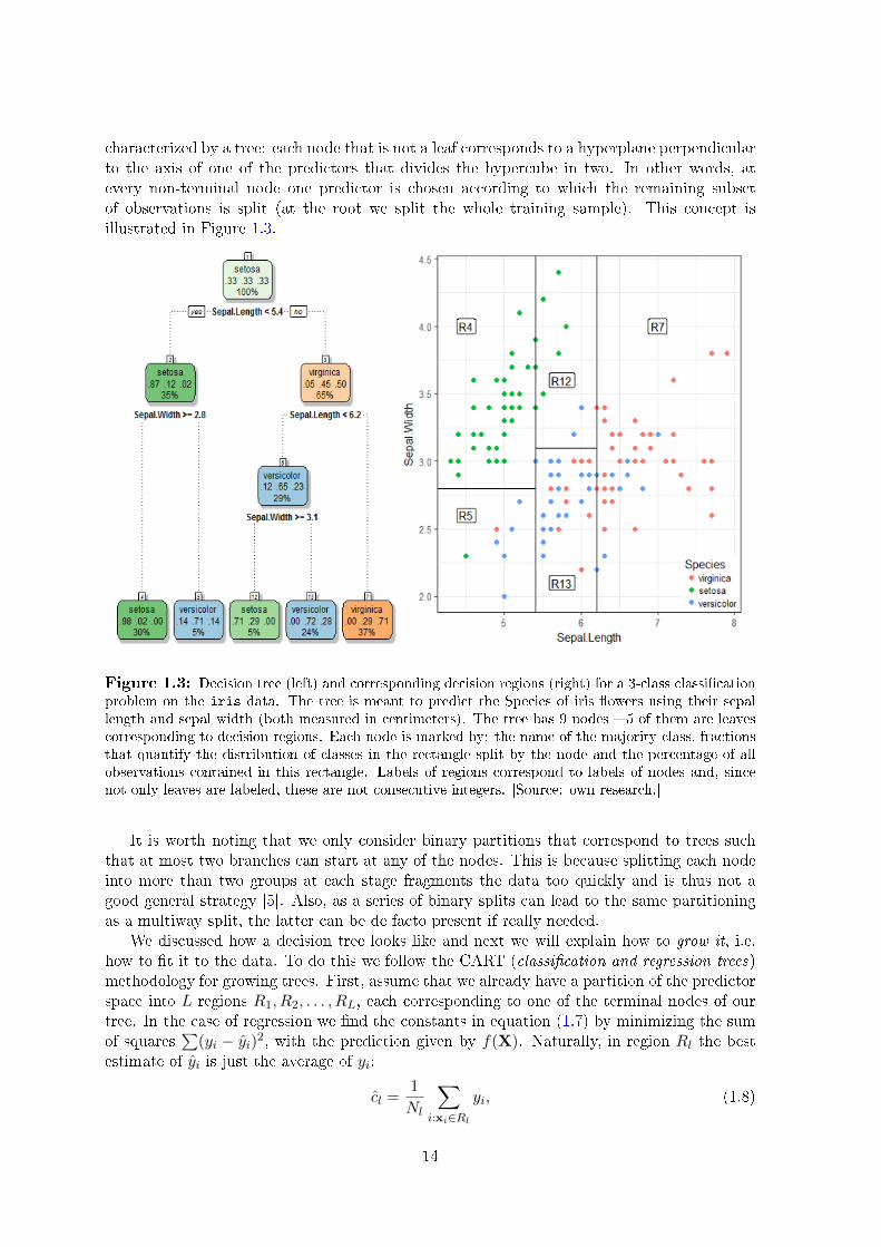
characterized by a tree: each node that is not a leaf corresponds to a hyperplane perpendicularto the axis of one of the predictors that divides the hypercube in two. In other words, atevery non-terminal node one predictor is chosen according to which the remaining subsetof observations is split (at the root we split the whole training sample). This concept isillustrated in Figure 1.3.

Figure 1.3: Decision tree (left) and corresponding decision regions (right) for a 3-class classicationproblem on the iris data. The tree is meant to predict the Species of iris owers using their sepallength and sepal width (both measured in centimeters). The tree has 9 nodes 5 of them are leavescorresponding to decision regions. Each node is marked by: the name of the majority class, fractionsthat quantify the distribution of classes in the rectangle split by the node and the percentage of allobservations contained in this rectangle. Labels of regions correspond to labels of nodes and, sincenot only leaves are labeled, these are not consecutive integers. [Source: own research.]

It is worth noting that we only consider binary partitions that correspond to trees suchthat at most two branches can start at any of the nodes. This is because splitting each nodeinto more than two groups at each stage fragments the data too quickly and is thus not agood general strategy [5]. Also, as a series of binary splits can lead to the same partitioningas a multiway split, the latter can be de facto present if really needed.

We discussed how a decision tree looks like and next we will explain how to grow it, i.e.how to t it to the data. To do this we follow the CART (classication and regression trees)methodology for growing trees. First, assume that we already have a partition of the predictorspace into L regions R1, R2, . . . , RL, each corresponding to one of the terminal nodes of ourtree. In the case of regression we nd the constants in equation (1.7) by minimizing the sumof squares

∑(yi − yi)2, with the prediction given by f(X). Naturally, in region Rl the best

estimate of yi is just the average of yi:

cl =1

Nl

∑i:xi∈Rl

yi, (1.8)

14

where Nl = |i : xi ∈ Rl| is the number of observations in region Rl. In the case ofclassication in order to minimize the number of misclassied observations, we classify allobservations from region Rl to the majority class k(l) = arg maxk plk, where plk is the estimateof E(Y = k|X), i.e. the proportion of observations in leave l that belong to class k:

plk =1

Nl

∑i:xi∈Rl

1(yi = k). (1.9)

Now we return to the question of how to nd the best binary partition of the predictorspace. We start at the root (with all the data) and consider splitting it on variable Xj at thesplit point s which denes a pair of half-planes corresponding to the left and right daughterof the root3:

RL(j, s) = X : Xj ≤ s, RR(j, s) = X : Xj > s. (1.10)

We pick Xj and s such that they solve:

minj,s

[mincL

NLQL(T ) + mincR

NRQR(T )

], (1.11)

where Ql(T ) measures the impurity of node l and is weighted by the number of observations inthis node. In general, Ql(T ) should measure how dierent are observations in node l as we areinterested in nding such a split that each node contains observations as similar as possibleso predicting the same value of response for them as in equation (1.7) will be accurate. Inpractice dierent measures of node impurity can be used and we need to select one suitableto our problem. For regression one usually uses the sum of squares:

Ql(T ) =1

Nl

∑i:xi∈Rl

(yi − cl)2. (1.12)

As a result, the inner minimization problems given in (1.11) are solved by averages of theresponse in both of the nodes as discussed before. The outer minimization can then be easilysolved as follows: we scan through Xj for j = 1, 2, . . . , p and for each variable nd the optimalsplit s to then determine the best pair (j, s). After nding the best split at the root we repeatthe above procedure to its daughters using their subsets of our sample and so on.

In the case of classication one usually uses one of the following node impurity measures:

• misclassication error: 1Nl

∑i:xi∈Rl

1(yi 6= k(l)) = 1− plk(l),

• Gini index:∑

k 6=k′ plkplk′ =∑K

k=1 plk(1− plk),

• cross-entropy or deviance: −∑K

k=1 plk log plk.

The above measures are all similar except for the fact that the misclassication error is notdierentiable so may be problematic when it comes to numerical optimization. In the end,the inner optimization problems are solved by (1.9) and to solve (1.11) we proceed as in theregression case.

3Note that this approach works only when the values of predictor Xj have a natural order, i.e. are eitherquantitative or qualitative and ordinal. Otherwise, inequalities with Xj are meaningless so we dene thehalf-planes in (1.10) in the following way: R1(j, C) = X : Xj ∈ C and R2(j, C) = X : Xj /∈ C for C ⊂ C,where C is the set of values taken by Xj . Of course, there are 2|C|−1 − 1 possible partitions of the set C intoC and Cc so the computations become prohibitive for large |C|.

15

A committee of trees

The main advantage of decision trees is that they can capture complex nonlinear relationsfound in the data due to their hierarchical structure the split of a set of observations in onenode is conditional on all splits occurring before, which is equivalent to modelling compositeinteractions. If grown suciently deep (i.e., such that each region of the predictor spacecontains observations with the same or very similar values of yi) trees produce estimates withlow bias but high variance, as the structure of a tree is very sensitive to minor changes in thedata [5].

Consequently, decision trees are natural candidates for averaging that could reduce vari-ance and at the same time keep bias low. Bagging or bootstrap aggregation is designed to dojust that: after drawing B bootstrap samples Z∗b of our training data (i.e., samples of thesame size as our data that are drawn uniformly with replacement) we grow a tree f∗b on eachof them and aggregate the result by taking the average in the case of regression and decidingby a majority vote in the case of classication. As all trees are identically distributed theexpectation of any one of them is the same as the expectation of their average, so baggingdoes not increase bias. The remaining question is whether it reduces the variance.

If the prediction of tree f∗b is a random variable Tb and T1, T2, . . . , TB are identicallydistributed with variance σ2 and the correlation between any two of them ρ := Cov(Ti, Tj)/σ

2

(for i 6= j) is positive, the variance of their average is equal to:

Var

(1

B

B∑b=1

Tb

)=

1

B2

BVar(T1) +∑i 6=j

Cov(Ti, Tj)

=

1

B2

Bσ2 +B∑i=1

B∑j 6=i

ρ√

Var(Ti) Var(Tj)

=

1

B2

(Bσ2 +B(B − 1)ρσ2

)= ρσ2 +

1− ρB

σ2. (1.13)

Thus, even as B goes to innity and the second term disappears the variance of our estimatoris determined by the size of correlation between bagged trees. Therefore, further variancereduction can be achieved by reducing the correlation between trees in such a way that thisis not oset by the increase in their individual variance. This idea is implemented in randomforests that use the following modication of bagging decision trees: when nding the optimalsplit at a given node we only consider a random subset of predictors. We can summarize thealgorithm of growing a random forest as follows4:

1. Draw a bootstrap sample Z∗b of size n from the training sample Z.

2. Grow a decision tree Tb on the bootstrap sample by repeating the following steps foreach node starting at the root until the terminal nodes contain observations with assimilar values of yi as possible:

(a) Draw independently and uniformly r out of p predictors, where r p.

(b) For each selected variable nd the best split point.

(c) Split the node into two daughter nodes using such variable and its optimal splitthat impurity of new nodes is lowest.

4It is worth noting that although in this paper we only consider regression and classication problems,random forests are also used in survival analysis where they are called random survival forests [9].

16

3. Repeat steps 1. and 2. for b = 1, 2, . . . , B producing the ensemble of tees TbBb=1.

4. Using predictions of individual trees predict the response for a new observation x:

Regression: y = 1B

∑Bb=1 Tb(x),

Classication: y = majority voteTb(x)Bb=1.

In practice, random forests to some extent reduce the variance of noisy estimates obtainedby decision trees while keeping the bias relatively low. Even more importantly, they are verysimple to use as they only require two tuning parameters r and B the choice of the latterdoes not change much as long as it is suciently big (see section 1.3.2). The other one isusually set by default to bp/3c for regression and b√pc for classication [5].

1.3.2. Analysis using random forests

Summary statistics

Due to their structure random forests provide summary statistics at three levels [19]:

1. Tree-level: as each tree is grown on its own bootstrap sample Z∗b it has its own test setcalled the out-of-bag (OOB) sample5 composed of observations that were not selectedinto Z∗b. Using the OOB sample for each tree we can compute an unbiased estimateof our prediction error that is almost identical to the one obtained by n-fold cross-validation [5] so this additional procedure is no longer necessary. Also, we can grow thetrees of our forest until this error stabilizes meaning that B is suciently big.

2. Variable-level: we can asses the importance of each predictor by randomly permuting itand observing the drop in accuracy of prediction of the forest.

3. Observation-level: for each observation the forest produces a distribution of predictionsacross all its trees so that we can identify observations for which prediction was unusuallyhard or easy as measured by how many trees predicted the response correctly.

These statistics make random forests interesting subjects of structure mining as one can comeup with dedicated techniques of knowledge extraction exploiting the structure of a forest andnot just rely on the general approaches presented in section 1.2 the "box" is not that "black"after all. In particular, we will discuss the variable-level summary statistics in greater detailin section 1.3.3.

Missing data

When it comes to missing data, random forests (and decision trees in general) oer twoapproaches in addition to the usual ones of either discarding observations that have missingvalues or lling in those values (e.g., with the mean for quantitative, median for qualitativeand ordinal, and mode for multinomial variables). The rst approach is to create a separatecategory "missing value" so this information can be used for splitting. Of course, this is only

5Observe that on average around one third of the sample is not selected to the bootstrap sample [10]. Thisstems from a simple calculation: we independently draw n observations from an n-element sample and if n islarge enough we use the following approximation:

P((xi, yi) /∈ Z∗b) =

(1− 1

n

)nn→∞−−−−→ 1

e≈ 0.368.

17

possible for qualitative variables but its combination with data imputation could be used forquantitative ones as well: we could ll in the missing values using the mean and create aseparate binary variable that points to the observations that had those values missing andinclude it as an additional predictor.

The second approach, distinctive for tree-based models, is to use surrogate splits whenevera value of the split variable is missing for an observation. Consider a split of variable Xj at thevalue sj if the value of Xj is missing for an observation i we choose another predictor Xj′ andits split point sj′ such that this new (surrogate) split best mimics the original one. Note thatwe can form an ordered list of surrogate splits for each node in case more predictor valuesare missing for some observations. To sum up, this approach exploits correlation betweenpredictors to make up for missing data so it will work best when this correlation is indeedhigh.

Imbalanced data

Another issue that may arise when using random forests concerns classication problems onimbalanced data meaning that at least one of the categories of the response variable is observedonly for a small number of observations. This is quite common in applications and is oftenaccompanied by the need of correct classication of the rare event (e.g., predicting default orfraud) which may not even appear in many bootstrap samples to which we t decision treeswhen building a forest so we may observe a bias in prediction towards more-common classes.Moreover, the algorithm treats all misclassications the same, whereas in such cases we areoften mainly interested in correct classication of the rare category.

In [4] Chen, Liaw and Breiman propose two ways of dealing with imbalanced data:

1. Weighted random forest (WRF) places a heavier penalty on misclassifying the minorityclass we assign a weight to each class (a larger one is given to the rare one) to thenuse them to weight the Gini criterion used for nding splits and nally to weight theshares of each class at terminal nodes to determine prediction of a tree.

2. Balanced random forest (BRF) modies the way of forming the bootstrap sample in thefollowing way: a bootstrap sample is drawn from the minority case and then the samenumber of cases is drawn from the majority case. This is an implementation of suchdown-sampling (i.e., reducing the size of the majority class in the bootstrap sample)that no information is lost as all observations from the majority class can appear in thebootstrap sample.

The authors corroborate the usefulness of the above methods with experiments on variousdata sets and both performed better than most other methods considered but none was foundto be unequivocally superior [16].

1.3.3. Importance of variables in a forest

In this paper we aim at explaining the structure of a random forest with a particular em-phasis on the importance of variables. We recognize the fact that in applications it is oftencritical to point to the variables that drive our prediction (otherwise it could be discardedas untrustworthy, see detailed discussion in [13]). To rise to this challenge we rst reviewexisting approaches of measuring variable importance in a random forest.

18

Perturbation of predictors

The rst approach to assessing importance of predictors in a random forest was proposed byBreiman in his paper [2] introducing the method and is still widely used today. It adopts theidea that if a variable plays a role in predicting our response, then perturbing it on the OOBsample should decrease prediction accuracy of our forest on this sample. Therefore, takingeach variable in turn, one can perturb its values and calculate the resulting average decreaseof predictive accuracy of the trees such a measure is sometimes referred to as VIMP, whichstands for variable importance.

Since the rst was introduced, two additional methods of permuting a predictor Xj havebeen proposed and together with Breiman's approach6 they form the following list:

(A) Permutation of the input the values of Xj in the OOB sample are randomly permuted.

(B) Random node assignment in each tree to assign the terminal value for an observationfollow split rules of the tree and if a split on Xj occurs than with equal probabilitieschoose the left or right daughter of this split.

(C) Opposite node assignment proceed similarly as in (B) but instead of randomly assigningthe left or right daughter choose the opposite one than would be normally chosen basedon the value of Xj for this observation.

All of the above measures are implemented in R: (A) is available in the benchmark packagerandomForest, whereas the newer package randomForestSRC allows for choosing among allthree perturbation methods. However, there are not a lot of theoretical results on the topic some are given in [7] in the case of regression and for method (B) modied in the followingway: if a split on Xj occurs than a random daughter is assigned not only at this split butalso for all subsequent ones even if they do not use Xj . The authors of the paper note thatthis is similar to methods (A)-(C) because for all four methods VIMP is directly aected bythe location of the rst split on Xj . On the other hand, the modication diers substantiallyfrom (A)-(C) importance measures as neither of them would be aected by an early split ona non-informative Xj that was selected for the split only due to chance as no informativepredictor was selected to the r variables considered for the split. Nevertheless, the resultspresented in [7] are instructive, in particular the authors prove that nodes closer to the rootcontribute more to prediction error this motivates the usefulness ofminimal depth, a measureof variable importance introduced in the next point.

Generally, perturbation of inputs as a measure of variable importance in random forestshas been widely criticized in the literature [1]. Most notably, when it comes to qualitativepredictors, VIMP measures are biased in favor of those that can take more categories. Theauthors of [17], who corroborate this criticism with simulations, ascribe this bias partly to theCART algorithm of growing trees as a solution they propose building random forests usingconditional inference trees [6] and incorporating a bias-correction into VIMP calculations(they implement this approach in the R package cforest).

Minimal depth

As mentioned before, variables used for splitting close to the root tend to be important asmeasured by VIMP. This has been proven in [7] using the concept of maximal subtrees, denedas follows: for each predictor Xj we call TXj an Xj-subtree of our tree T if the root of TXj is

6The Breiman's approach is sometimes called the Breiman-Cutler permutation VIMP.

19

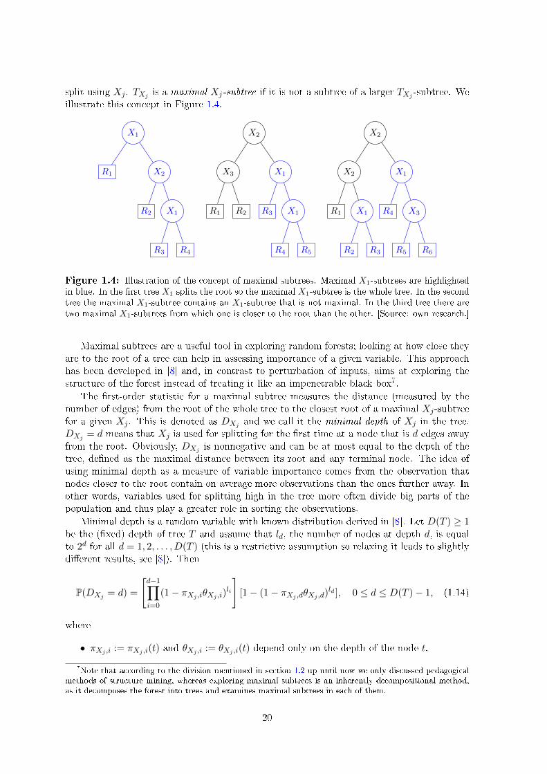
split using Xj . TXj is a maximal Xj-subtree if it is not a subtree of a larger TXj -subtree. Weillustrate this concept in Figure 1.4.

X1

R1 X2

R2 X1

R3 R4

X2

X3

R1 R2

X1

R3 X1

R4 R5

X2

X2

R1 X1

R2 R3

X1

R4 X3

R5 R6

Figure 1.4: Illustration of the concept of maximal subtrees. Maximal X1-subtrees are highlightedin blue. In the rst tree X1 splits the root so the maximal X1-subtree is the whole tree. In the secondtree the maximal X1-subtree contains an X1-subtree that is not maximal. In the third tree there aretwo maximal X1-subtrees from which one is closer to the root than the other. [Source: own research.]

Maximal subtrees are a useful tool in exploring random forests; looking at how close theyare to the root of a tree can help in assessing importance of a given variable. This approachhas been developed in [8] and, in contrast to perturbation of inputs, aims at exploring thestructure of the forest instead of treating it like an impenetrable black box7.

The rst-order statistic for a maximal subtree measures the distance (measured by thenumber of edges) from the root of the whole tree to the closest root of a maximal Xj-subtreefor a given Xj . This is denoted as DXj and we call it the minimal depth of Xj in the tree.DXj = d means that Xj is used for splitting for the rst time at a node that is d edges awayfrom the root. Obviously, DXj is nonnegative and can be at most equal to the depth of thetree, dened as the maximal distance between its root and any terminal node. The idea ofusing minimal depth as a measure of variable importance comes from the observation thatnodes closer to the root contain on average more observations than the ones further away. Inother words, variables used for splitting high in the tree more often divide big parts of thepopulation and thus play a greater role in sorting the observations.

Minimal depth is a random variable with known distribution derived in [8]. Let D(T ) ≥ 1be the (xed) depth of tree T and assume that ld, the number of nodes at depth d, is equalto 2d for all d = 1, 2, . . . , D(T ) (this is a restrictive assumption so relaxing it leads to slightlydierent results, see [8]). Then

P(DXj = d) =

[d−1∏i=0

(1− πXj ,iθXj ,i)li

][1− (1− πXj ,dθXj ,d)ld ], 0 ≤ d ≤ D(T )− 1, (1.14)

where

• πXj ,i := πXj ,i(t) and θXj ,i := θXj ,i(t) depend only on the depth of the node t,

7Note that according to the division mentioned in section 1.2 up until now we only discussed pedagogicalmethods of structure mining, whereas exploring maximal subtrees is an inherently decompositional method,as it decomposes the forest into trees and examines maximal subtrees in each of them.

20

• πXj ,i(t) is the probability that Xj is selected as one of the r candidates for splittingnode t at depth i, assuming there is no maximal Xj-subtree with depth lower than i,

• θXj ,i(t) is the probability that Xj splits the node t with depth i, assuming that Xj is acandidate for splitting t and there is no maximal Xj-subtree with depth lower than i.

It is important to realize that the sum of probabilities (1.14) over d is bounded between 0 and1 but does not equal 1 when no maximal Xj-subtree exists. In such a case we set DXj to thedepth of the tree:

P(DXj = D(T )) = 1−D(T )−1∑d=1

P(DXj = d). (1.15)

Now we can easily calculate the minimal depth of variables X1, X2, X3 in trees presented inFigure 1.4:

• X1 has minimal depth 0 in the rst tree and 1 in the others,

• X2 has minimal depth 1 in the rst tree and 0 in the others,

• X3 is not used for splitting in the rst tree so its minimal depth there is 3, it is equalto 1 in the second tree and 2 in the third.

It must be remembered that the concept of minimal depth strongly relies on the existence ofmaximal subtrees with respect to predictors whose importance we want to measure. Therefore,in problems with small n and big p we observe a "ceiling eect" of minimal depth as the treescannot be grown deep enough to suciently dierentiate the statistic between variables8.

Node impurity

The third popular approach to measuring variable importance in random forests is based onnode impurity measures that are used for growing trees (see section 1.3.1). Recall that ateach split potential improvement of node purity is calculated for all candidate variables andwe select for splitting the one which maximizes this improvement. Therefore, we can measureimportance of each predictor by calculating its improvement in the split-criterion accumulatedover all trees. This idea is easily implemented as one only needs to store the information onnode purity calculated in the tree-growing process and aggregate it for each predictor.

In the case of classication problems, in which Gini index is the most widely used impuritymeasure, many studies found that measuring variable importance with this index induces biasin cases where the values of a predictor cluster into well separated groups regardless of whetherthe predictor is qualitative of quantitative [1]. Some procedures of correcting this bias havebeen proposed: e.g., permutation importance (PIMP) which normalizes the biased importancemeasure using a permutation test and additionally reports a p-value for each variable (see [1]).

8One solution to this issue has been proposed in [8]: RSF-Variable Hunting, which is a regularized algorithmfor random survival forests.

21

Chapter 2

Functionality of the R package

randomForestExplainer

In this chapter I introduce my new R package randomForestExplainer devoted to exploringimportance of variables in a random forest. The package is designed for forests built withthe randomForest package, which I consider the most popular implementation of the randomforest algorithm. Functionality of my package is mainly concerned with visualization and forthat purpose it uses ggplot2 and two other packages that build upon it: GGally and ggrepel.For data processing and aggregation I use data.table, dplyr, dtplyr, DT and reshape2.Finally, for creating automatic summaries of forests in the form of HTML documents I usermarkdown.

Each section of this chapter is devoted to discussing a dierent functionality of the pack-age1. Every section starts with general ideas that I implement, then lists the functions tonally describe in detail how they work. For brevity I present my functions using pseudocode the R code can be found in the online repository of the package2. I divide most of myfunctions into three groups:

1. Data-generating the function takes as its main argument a randomForest object andreturns data that are potentially useful to the user, e.g. importance measures.

2. Plotting the function takes as its main argument a result of some data-generatingfunction and plots it using ggplot2.

3. Auxiliary the function is a building block of a function from group 1. or 2. and is notdirectly available to users of the package.

Note that this division separates data from plots so when the user wants to visualize someresult, she usually has to generate appropriate data rst. This may seem onerous, but it isuseful as the user only needs to generate the data once (and for large random forests this maybe time-consuming) to then plot it multiple times while adjusting graphical parameters.

Apart from describing how the functions work I illustrate the plotting ones using a ran-dom forest build on the iris data that predicts the Species of an iris ower using its fournumerical characteristics: sepal and petal length and width. I grow the forest using therandomForest::randomForest function with option localImp set to TRUE.

1The division into sections corresponds to the division of R code that makes up randomForestExplainer

into separate les.2See https://github.com/geneticsMiNIng/BlackBoxOpener/tree/master/randomForestExplainer.

23

2.1. Minimal depth distribution

In section 1.3.3 I introduced the concept of minimal depth and discussed its usefulness. Inpractice, calculating minimal depth is implemented in the randomForestSRC package, which inaddition to what randomForest does allows for building random survival forests. To comparevariables, mean minimal depth over all trees is calculated, leading to a ranking of predictorsfrom lowest (best) to highest (worst) mean minimal depth.

In my opinion looking only at the mean is not always sucient and there is much to begained from analyzing the whole distribution of minimal depth. I implement this idea inrandomForestExplainer using the following functions:

(1) calculate_tree_depth (auxiliary) takes a data frame describing a single decision treeand adds to it information about depth of each node,

(2) min_depth_distribution (data-generating) for each tree in a forest the function com-putes depth of predictors using (1), gathers results for all trees in one data frame andcomputes the minimum of depth of each variable in each tree,

(3) min_depth_count (auxiliary) takes the result of (2) and counts the instances of eachminimal depth for each variable and the number of trees in which each variable occurred;it also computes the mean tree depth in the forest,

(4) get_min_depth_means (auxiliary) takes results of (2) and (3), and calculates meanminimal depth for each variable in one of three possible ways specied by the user,

(5) plot_min_depth_distribution (plotting) takes the result of (2) to plot the discretedistribution of minimal depth obtained with (3) for a certain number of variables withthe lowest mean minimal depth as given by (4); mean values are also added to the plot.

In this section I describe each of the above functions in turn.

2.1.1. Calculate the distribution

Let forest be my random forest produced by the package randomForest with option localImp= TRUE. To get a data frame with split information on the b-th tree, where variables are codedwith their labels instead of numbers, I use the function randomForest::getTree(forest, k

= b, labelVar = TRUE) and store the result in frame.Each row in frame corresponds to a node in my tree and the rst two entries point to the

left and right daughter of this node using names of their respective rows; the third entry is thename of the predictor used for splitting. Conveniently, the rows in frame are ordered in sucha way that daughters are always below their parents. This leads to a very simple constructionof the function calculate_tree_depth described in Algorithm 2.1.

Algorithm 2.1: Calculating depth of nodes in a single tree

Function: calculate_tree_depth(frame)

let r ← number of rows of frame

let depth ← vector of length rlet depth[1] ← 0for i = 2, 3, . . . , r

begin

find j such that: left daughter[j] = i or right daughter[j] = ilet depth[i] ← depth[j] + 1

end

24

Return: frame with depth as a new column

Once I am able to calculate depth of nodes in a single tree it is easy to do that for the wholeforest by taking all its trees in turn and applying calculate_tree_depth. Then, for eachtree and predictor used in it for splitting I calculate the minimum of its depth. This simpleprocedure is implemented in the function min_depth_distribution described in Algorithm2.2 the function takes forest as its argument and returns a data frame with the wholedistribution of minimal depth.

Algorithm 2.2: Calculating minimal depth in every tree of a forest

Function: min_depth_distribution(forest)

let forest_table ← empty data frame

for b = 1, 2, . . . , Bbegin

let frame ← getTree(forest, k = b, labelVar = TRUE)

add calculate_tree_depth(frame) to forest_table

end

group forest_table by: tree, split variable

let min_depth_frame ← min(depth) in each group

Return: min_depth_frame

To prepare the data frame min_depth_frame containing the distribution for plotting andaveraging, I use the function min_depth_count (Algorithm 2.3) that returns a list with threeelements: a data frame with frequency counts of each minimal depth for each variable, a dataframe that for each variable gives the number of trees in which it was used for splitting andthe mean depth of a tree in the forest.

Algorithm 2.3: Count the trees in which each variable had a given minimal depth

Function: min_depth_count(min_depth_frame)

/* Count instances of each minimal depth */

group min_depth_frame by: variable, minimal_depth

let min_depth_count ← count observations in each group

/* Count number of trees in which each variable occured */

group min_depth_count by: variable

let occurrences ← sum(count) in each group

/* Calculate mean depth of a tree */

group min_depth_frame by: tree

let mean_tree_depth ← mean[max(minimal_depth) + 1 in each group]

Return: list of min_depth_count, occurrences, mean_tree_depth

2.1.2. Mean minimal depth

Although my main goal in this section is to look at the whole distribution of minimal depth,calculating its mean is useful as it gives a simple ranking of variables. Such a ranking can beused for selecting the subset of variables of which the minimal depth distribution we wish toplot. Moreover, while considering the whole distribution, I should also look at the means tosee whether they indeed provide insucient information about my variables.

I propose two ways of calculating mean minimal depth in addition to the one describedin section 1.3.3. All three approaches dier in he way they treat missing values that appearwhen a variable is not used for splitting in a tree. They can be described as follows:

25

(I) Filling missing values: the minimal depth of a variable in a tree that does not use it forsplitting is equal to the mean depth of trees3 in the forest [8].

(II) Restricting the sample: to calculate the mean minimal depth only B out of B observa-tions are considered, where B is equal to the maximum number of trees in which anyvariable was used for splitting. Remaining missing values for variables that were usedfor splitting less than B times are lled in as in (I).

(III) Ignoring missing values: mean minimal depth is calculated using only non-missing val-ues.

Obviously, the results obtained using each of those approaches dier whenever many valuesare missing. One notable example of this occurs when the data contain many variables butfew observations (large p, small n) as this leads to shallow trees, each using only a fraction ofall p variables for splitting.

The main advantage of calculating mean minimal depth using (I) is the fact that it in-creases the mean for variables that are not frequently used for splitting. However, when themajority of values are missing the means will be strongly pulled towards mean depth of treesin the forest leading to small variability of the mean between predictors and problems withinterpretation of these inated values (in section 1.3.3 I referred to this as the "ceiling eect").The second approach aims at reducing this eect by imputing only as many observations asnecessary to use samples of the same size for all variables to compute the mean. One drawbackof both (I) and (II) is that the value used for lling missing values is somewhat articial.

Finally, approach (III) to calculating mean minimal depth only uses available observationsand discards missing data. This removes the concern of lling missing values with somethingthat is not really variable depth and therefore distorts interpretability of the mean. However,a major drawback of this approach is that low values of mean minimal depth obtained in thisway do not necessarily mean that a variable is important. On the contrary: when a variable isused for splitting only once in a forest and this happens at the root (e.g. because no importantvariables were selected as candidates for the split) its mean minimal depth will be equal tozero, the lowest possible value.

In my opinion each of the three methods may be useful in applications so whenever Icalculate the minimal depth I ask the user to specify the parameter mean_sample as equalto one of the following: "all_trees", "top_trees", "relevant_trees" corresponding tomethods (I), (II) and (III) (I set "top_trees" as the default).

After obtaining min_depth_frame using the function min_depth_distribution and sav-ing the result of min_depth_count as count_list I need to calculate means of minimal depthof my variables as described above. To do this I create the function get_min_depth_means

described in Algorithm 2.4.

Algorithm 2.4: Calculate means of minimal depth in one of three ways

Function: get_min_depth_means(min_depth_frame, count_list, mean_sample)

if mean_sample = "all_trees"

begin

for j such that: minimal_depth[j] is missing

begin

let minimal_depth[j] ← mean_tree_depth

end

3Note that the depth of a tree is equal to the length of the longest path from root to leave in this tree.This equals the maximum depth of a variable in this tree plus one, as leaves are by denition not split by anyvariable.

26

group min_depth_frame by: variable

let min_depth_means ← mean(minimal_depth) in each group

end

if mean_sample = "top_trees"

begin

for j such that: minimal_depth[j] is missing

begin

let count[j] ← count[j] − min(count[all j])let minimal_depth[j] ← mean_tree_depth

end

group min_depth_count by: variable

let min_depth_means ← mean(minimal_depth, weights = count) in each group

end

if mean_sample = "relevant_trees"

begin

for j such that: minimal_depth[j] is missing

begin

remove observation jend

group min_depth_frame by: variable

let min_depth_means ← mean(minimal_depth) in each group

end

Return: min_depth_means

2.1.3. Plot the distribution

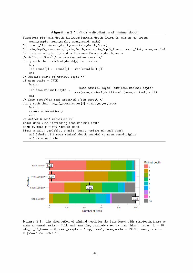
Finally, I create the function plot_min_depth_distribution for plotting the minimal depthdistribution (Algorithm 2.5). Its arguments are:

• min_depth_frame produced by the data-generating function min_depth_distribution,

• k the maximal number of variables with lowest mean minimal depth to be includedin the plot,

• min_no_of_trees the minimal number of trees in which a variable has to be used forsplitting to be used for plotting,

• mean_sample the type of sample on which to calculate mean minimal depth,

• mean_scale logical: should the mean minimal depth be rescaled so that its minimumand maximum are equal to 0 and 1, respectively?

• mean_round integer: number of digits to which the displayed mean minimal depthshould be rounded,

• main the title of the plot.

The function plots the discrete distribution of minimal depth for at most k variables withlowest mean minimal and in addition displays this statistic (see Figure 2.1). As I mentionedbefore, in some applications it might be the case that the minimal depth distribution isdominated by missing values. Then, including missing values in the plot could obscure therest of the distribution. To avoid that for each variable we only plot the number of missingvalues in addition to the minimal number of missing values (B − B).

27

Algorithm 2.5: Plot the distribution of minimal depth

Function: plot_min_depth_distribution(min_depth_frame, k, min_no_of_trees,

mean_sample, mean_scale, mean_round, main)

let count_list ← min_depth_count(min_depth_frame)

let min_depth_means ← get_min_depth_means(min_depth_frame, count_list, mean_sample)

let data ← min_depth_count with means from min_depth_means

/* Subtract B − B from missing values count */

for j such that: minimal_depth[j] is missing

begin

let count[j] ← count[j] − min(count[all j])end

/* Rescale means of minimal depth */

if mean_scale = TRUE

begin

let mean_minimal_depth ← mean_minimal_depth− min(mean_minimal_depth)

max(mean_minimal_depth)− min(mean_minimal_depth)end

/* Keep variables that appeared often enough */

for j such that: no_of_occurrences[j] < min_no_of_trees

begin

remove observation jend

/* Select k best variables */

order data with increasing mean_minimal_depth

keep at most k first rows of data

Plot: y-axis: variable, x-axis: count, color: minimal_depth

add labels with mean_minimal_depth rounded to mean_round digits

add main as title

Figure 2.1: The distribution of minimal depth for the iris forest with min_depth_frame asmain argument, main = NULL and remaining parameters set to their default values: k = 10,min_no_of_trees = 0, mean_sample = "top_trees", mean_scale = FALSE, mean_round =2. [Source: own research.]

28

2.2. Variable importance

In this section I introduce the part of randomForestExplainer functionality that calculatesand plots various variable importance measures using the following functions:

(1) measure_importance (data-generating) takes forest and generates a data frame con-taining various variable importance measures,

(2) important_variables takes the result of (1) and returns names of up to k top variablesaccording to the sum of rankings based on specied importance measures,

(3) plot_multi_way_importance (plotting) takes the result of (1) and plots two or threevariable importance measures against each other (two corresponding to y and x coordi-nates and the optional third to the size or color of points),

(4) plot_importance_ggpairs (plotting) takes the result of (1) and plots all pairs of se-lected variable importance measures against each other,

(5) plot_importance_rankings (plotting) takes the result of (1) and plots all pairs ofrankings based on selected variable importance measures against each other.

First, I need to calculate various variable importance measures. In Algorithm 2.6 I describethe function measure_importance that takes our forest, gathers split information on all itstrees in a forest_table and calculates the following importance measures for each variableXj :

(a) accuracy_decrease (classication) mean decrease of prediction accuracy after Xj ispermuted,

(b) gini_decrease (classication) mean decrease in the Gini index of node impurity (i.e.increase of node purity) by splits on Xj ,

(c) mse_increase (regression) mean increase of mean squared error after Xj is permuted,

(d) node_purity_increase (regression) mean node purity increase by splits on Xj , asmeasured by the decrease in sum of squares,

(e) mean_minimal_depth mean minimal depth calculated in one of three ways speciedby the parameter mean_sample, as described in section 2.1.2,

(f) no_of_trees total number of trees in which a split on Xj occurs,

(g) no_of_nodes total number of nodes that use Xj for splitting (it is usually equal tono_of_trees if trees are shallow),

(h) times_a_root total number of trees in which Xj is used for splitting the root node(i.e., the whole sample is divided into two based on the value of Xj),

(i) p_value p-value for the one-sided binomial test using the following distribution:

Bin(no_of_nodes, P(node splits on Xj)), (2.1)

where I calculate the probability of split on Xj as if Xj was uniformly drawn from ther candidate variables

P(node splits on Xj) = P(Xj is a candidate) · P(Xj is selected) =r

p· 1

r=

1

p. (2.2)

29

This test tells me whether the observed number of successes (number of nodes in whichXj was used for splitting) exceeds the theoretical number of successes if they wererandom (i.e. following the binomial distribution (2.1)).

Measures (a)-(d) are calculated by the randomForest package (see [12]) so need only to beextracted from my forest object if option localImp = TRUE was used for growing the forest(I assume this is the case). Note that measures (a) and (c) are based on the decrease inpredictive accuracy of the forest after perturbation of the variable, (b) and (d) are based onchanges in node purity after splits on the variable and (e)-(i) are based on the structure ofthe forest.

Algorithm 2.6: Calculate variable importance measures

Function: measure_importance(forest, mean_sample)

/* Extract randomForest importance measures */

if forest type = "classification"

begin

let accuracy_decrease ← MeanDecreaseAccuracy from forest importance

let gini_decrease ← MeanDecreaseGini from forest importance

let vimp_frame ← accuracy_decrease and gini_decrease

end

if forest type = "regression"

begin

let mse_increase ← %IncMSE from forest importance

let node_purity_increase ← IncNodePurity from forest importance

let vimp_frame ← mse_increase and node_purity_increase

end

/* Calculate structure importance measures */

let forest_table ← empty data frame

for b = 1, 2, . . . , Bbegin

let frame ← getTree(forest, k = b, labelVar = TRUE)

add calculate_tree_depth(frame) to forest_table

end

group forest_table by: tree, split variable

let min_depth_frame ← min(depth) in each group

min_depth ← get_min_depth_means(min_depth_frame, min_depth_count(min_depth_frame),

mean_sample)

group forest_table by: split variable

let no_of_nodes ← count observations in each group

group min_depth_frame by: variable

let no_of_trees ← count observations in each group

/* Calculate p-value */

let p_value ← p-value of right-sided binomial test:

number of successes: no_of_nodes

number of trials: sum(no_of_nodes)

probability of success: 1/pReturn: data frame with vimp_frame, min_depth, no_of_nodes, no_of_trees, p_value

After calculating all variable importance measures I might be interested in nding a num-ber of top variables according to one or more of those measures (e.g., to restrict further analysisto this subset of variables). I propose a simple solution of doing that: selecting variables withthe lowest sum of rankings (index), each based on one of the importance measures of interest.This is implemented in the function important_variables (Algorithm 2.7) that takes as itsargument the result of measure_importance, a vector of importance measures to be used,

30

the number of top variables to select and a ties_action parameter. The last species whichvariables should be selected if a problematic tie occurs, i.e. when the k-th top variable hassum of rankings q and this is equal to that of the k+1-th variable. Three possible values ofthis parameter are:

• none no variable with index=q is included in the result so it may be shorter than k,

• all all variables with index=q are included in the result so it may be longer than k,

• draw a uniformly drawn subset of variables with index=q appears in the result so itwill be exactly of length k.

Algorithm 2.7: Select k most important variables in a forest

Function: important_variables(importance_frame, k, measures, ties_action)

let rankings ← rank variables according to measures

let index ← sum(rankings)

let vars ← min(k, p) variables with lowest index

let q ← index[j] for j such that: index[j] = max(index[l ∈ vars])

if [#(j such that: index[j] = q) > 1] and [#(j such that: index[j] ≤ q) > k]

begin

if ties_action = "none" then let vars ← j such that: index[j] < qif ties_action = "all" then let vars ← j such that: index[j] ≤ qif ties_action = "draw"

begin

let vars ← j such that: index[j] < qadd to vars: uniformly draw k−#(vars) j's such that: index[j] = qend

end

Return: vars (a vector of variable names)

Figure 2.2: The multi-way importance plot for the iris forest with importance_frame asmain argument, size_measure = "accuracy_decrease", main = NULL and the remaining parame-ters set to their default values: x_measure = "mean_min_depth", y_measure = "times_a_root",

min_no_of_trees = 0, no_of_labels = 10. [Source: own research.]

Regardless of the type of my random forest, the result of measure_importance containsseven importance measures for the predictors, which opens a lot of possibilities for visual-

31

ization. I propose three plotting functions in turn in all of them, in addition to tuningparameters discussed below, the user can supply a character string main to be used as title.

The rst plotting function produces what I call a multi-way importance plot that showsthree selected measures using a scatter plot with size or color of points varying according tothe third measure (see Figure 2.2). The corresponding function plot_multi_way_importance

takes the following parameters:

• importance_frame the result of measure_importance,

• x_measure, y_measure, size_measure each is a string containing one of importancemeasures contained in importance_frame; size_measure is optional,

• min_no_of_trees the minimal number of trees in which a variable has to be used forsplitting to appear in the plot,

• no_of_labels the number of top variables, according to all measures plotted, to belabeled (we allow for more labels in case of ties).

The resulting plot is slightly dierent depending on which measures are being plotted. Ifno_of_nodes, no_of_trees or times_a_root are used as either x_measure or y_measure thecorresponding axis uses the square root scale so that dierences in high values are clearlyvisible (as these are usually the most interesting). When it comes to size_measure: if itis set to mean_min_depth its scale is reversed so that bigger points correspond to smallervalues (as variables with smaller mean minimal depth are considered better). Furthermore,if p_value is the size_measure, then instead of varying the size of points I vary their colorafter turning p_value into a qualitative variable informing of the level of signicance at whicheach predictor is signicant this modication makes the plot a lot easier to analyze.

Figure 2.3: Pairwise comparisons of importance measures of variables for the iris forest withimportance_frame as main argument, main = NULL and the measures argument set to its defaultnames(importance_frame)[c(2, 4, 5, 3, 7)]. [Source: own research.]

32

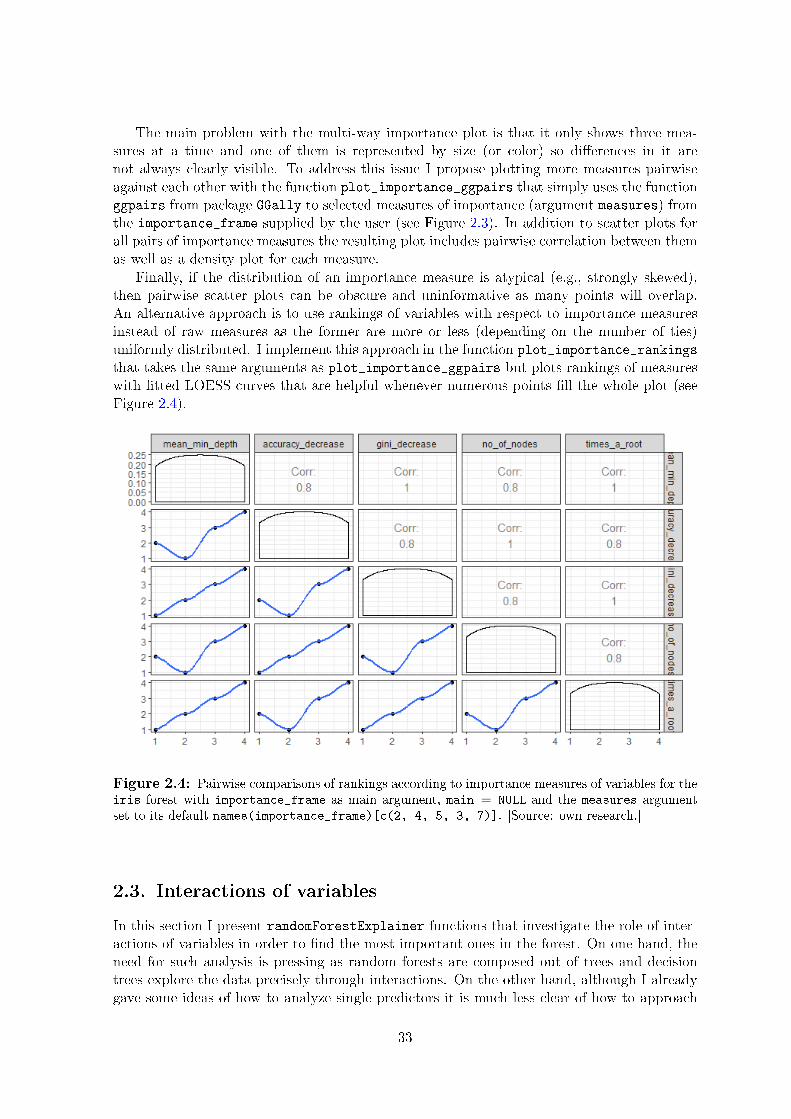
The main problem with the multi-way importance plot is that it only shows three mea-sures at a time and one of them is represented by size (or color) so dierences in it arenot always clearly visible. To address this issue I propose plotting more measures pairwiseagainst each other with the function plot_importance_ggpairs that simply uses the functionggpairs from package GGally to selected measures of importance (argument measures) fromthe importance_frame supplied by the user (see Figure 2.3). In addition to scatter plots forall pairs of importance measures the resulting plot includes pairwise correlation between themas well as a density plot for each measure.

Finally, if the distribution of an importance measure is atypical (e.g., strongly skewed),then pairwise scatter plots can be obscure and uninformative as many points will overlap.An alternative approach is to use rankings of variables with respect to importance measuresinstead of raw measures as the former are more or less (depending on the number of ties)uniformly distributed. I implement this approach in the function plot_importance_rankings

that takes the same arguments as plot_importance_ggpairs but plots rankings of measureswith tted LOESS curves that are helpful whenever numerous points ll the whole plot (seeFigure 2.4).

Figure 2.4: Pairwise comparisons of rankings according to importance measures of variables for theiris forest with importance_frame as main argument, main = NULL and the measures argumentset to its default names(importance_frame)[c(2, 4, 5, 3, 7)]. [Source: own research.]

2.3. Interactions of variables

In this section I present randomForestExplainer functions that investigate the role of inter-actions of variables in order to nd the most important ones in the forest. On one hand, theneed for such analysis is pressing as random forests are composed out of trees and decisiontrees explore the data precisely through interactions. On the other hand, although I alreadygave some ideas of how to analyze single predictors it is much less clear of how to approach

33

their interactions. Usually, this is done by adjusting the concept of importance of single vari-ables such that it would allow for interactions. I do this in the case of minimal depth byintroducing conditional minimal depth. In addition, I examine the prediction of our randomforest for a grid of values of an interaction of two numerical variables. I do this using thefollowing functions:

(1) conditional_depth (auxilliary) takes a data frame describing a single decision tree(after depths of nodes have been calculated with calculate_tree_depth), a vector ofconditioning variables and returns the data frame with information on depth of nodesconditional on each of the conditioning variables,

(2) min_depth_interactions_values (auxilliary) takes a random forest, a vector of condi-tioning variables and uses (1) to compute conditional depth in the whole forest to thencalculate the minimum for each variable in each tree and return it in a list together withmean depths of maximal subtrees with respect to each conditioning variable,

(3) min_depth_interactions (data-generating) takes a random forest and a vector of con-ditioning variables, uses (2) to compute conditional minimal depth in all trees and meandepths of maximal subtrees, and returns a data frame with mean conditional minimaldepth for each interaction calculated in one of three ways,

(4) plot_min_depth_interactions (plotting) takes the result of (3) and plots the condi-tional mean minimal depth for a given number of most frequent interactions togetherwith mean minimal depth of the second variable in the interaction, for comparison,

(5) plot_predict_interaction uses the forest and data on which it was trained to plotits prediction for each point on a grid for two numerical predictors with values of otherpredictors sampled from their empirical distributions.

It is worth noting that exploring interactions is usually computationally intensive due to manypossibilities (for p variables there are 1/2p(p − 1) possible interactions of two variables) so Irestrict my analysis to interactions of two variables.

2.3.1. Conditional minimal depth

Conditional minimal depth is a simple modication of minimal depth: for a conditioningvariable Xj and a second variable Xl I dene conditional minimal depth of Xl with respect to

Xj as the minimal depth of Xl in the maximal Xj-subtree closest to the root of the wholetree minus one (my denition is based on the ideas presented in [8]). I subtract one in orderto make the values of conditional minimal depth comparable to the unconditional ones: thelatter range from zero, whereas without subtracting one the former would range from one asthe root of any Xj-subtree is by denition split on Xj .

Obviously, conditional minimal depth is not symmetric: if Xj is the conditioning variableI analyze Xj-subtrees and look for splits on Xl in them, whereas if I exchange the roles ofthese variables I would be examining Xl-subtrees. As an example consider the simple decisiontrees in Figure 1.4 and variables X2 and X3. In the second and third trees X3 is always belowX2 so conditional minimal depth of X3 with respect to X2 is equal to 1 and 2, respectively.On the other hand, the conditional minimal depth of X2 with respect to X3 is equal to themean depth of maximal X3-subtrees in the forest as there are no splits on X2 in X3-subtrees.

This leads to the conclusion that analyzing conditional minimal depth makes much moresense if the conditioning variables are often used for splitting in the forest, because then I

34

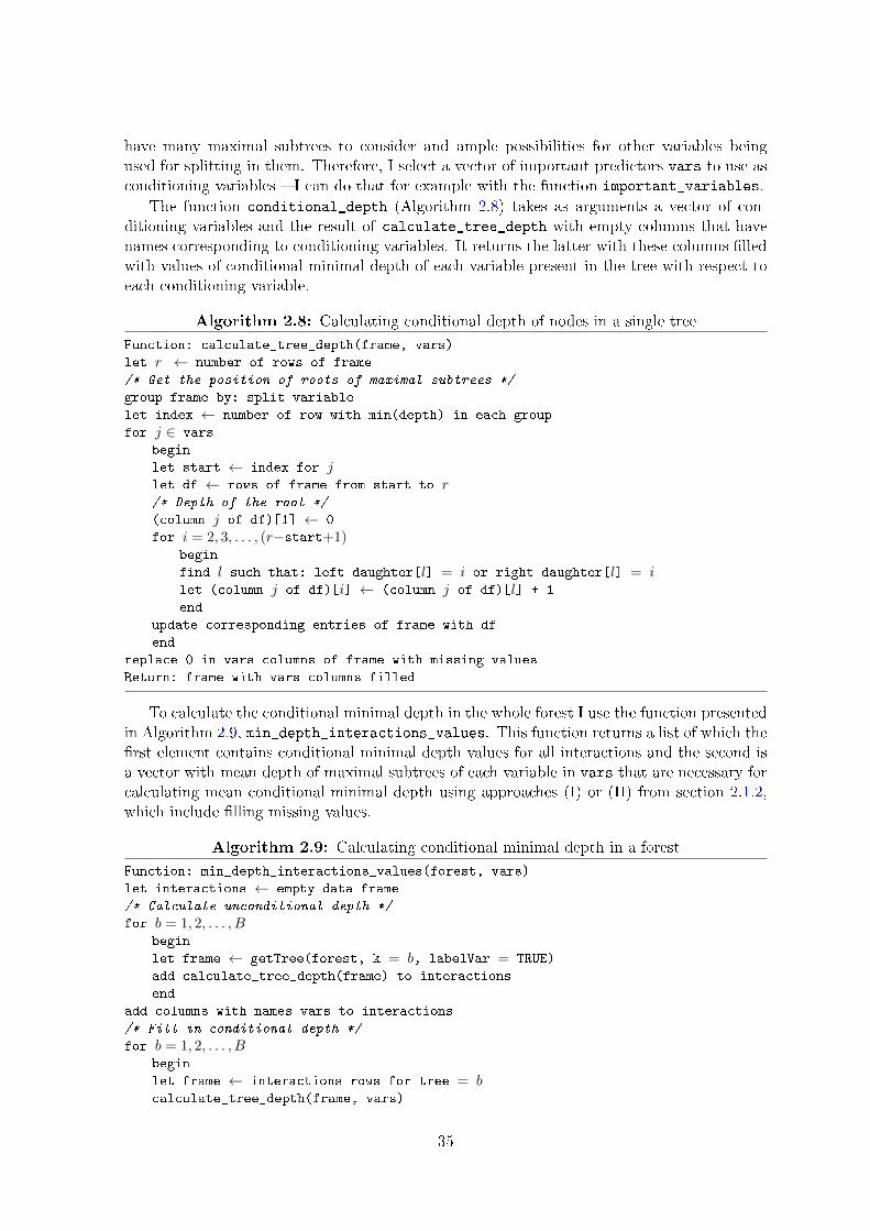
have many maximal subtrees to consider and ample possibilities for other variables beingused for splitting in them. Therefore, I select a vector of important predictors vars to use asconditioning variables I can do that for example with the function important_variables.

The function conditional_depth (Algorithm 2.8) takes as arguments a vector of con-ditioning variables and the result of calculate_tree_depth with empty columns that havenames corresponding to conditioning variables. It returns the latter with these columns lledwith values of conditional minimal depth of each variable present in the tree with respect toeach conditioning variable.

Algorithm 2.8: Calculating conditional depth of nodes in a single tree

Function: calculate_tree_depth(frame, vars)

let r ← number of rows of frame

/* Get the position of roots of maximal subtrees */

group frame by: split variable

let index ← number of row with min(depth) in each group

for j ∈ vars

begin

let start ← index for jlet df ← rows of frame from start to r/* Depth of the root */

(column j of df)[1] ← 0

for i = 2, 3, . . . , (r−start+1)begin

find l such that: left daughter[l] = i or right daughter[l] = ilet (column j of df)[i] ← (column j of df)[l] + 1

end

update corresponding entries of frame with df

end

replace 0 in vars columns of frame with missing values

Return: frame with vars columns filled

To calculate the conditional minimal depth in the whole forest I use the function presentedin Algorithm 2.9, min_depth_interactions_values. This function returns a list of which therst element contains conditional minimal depth values for all interactions and the second isa vector with mean depth of maximal subtrees of each variable in vars that are necessary forcalculating mean conditional minimal depth using approaches (I) or (II) from section 2.1.2,which include lling missing values.

Algorithm 2.9: Calculating conditional minimal depth in a forest

Function: min_depth_interactions_values(forest, vars)

let interactions ← empty data frame

/* Calculate unconditional depth */

for b = 1, 2, . . . , Bbegin

let frame ← getTree(forest, k = b, labelVar = TRUE)

add calculate_tree_depth(frame) to interactions

end

add columns with names vars to interactions

/* Fill in conditional depth */

for b = 1, 2, . . . , Bbegin

let frame ← interactions rows for tree = bcalculate_tree_depth(frame, vars)

35

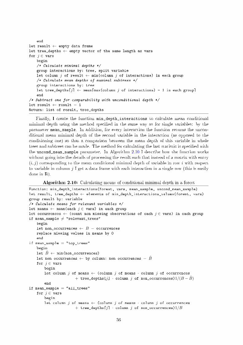
end

let result ← empty data frame

let tree_depths ← empty vector of the same length as vars

for j ∈ vars

begin

/* Calculate minimal depths */

group interactions by: tree, split variable

let column j of result ← min(column j of interactions) in each group

/* Calculate mean depths of maximal subtrees */

group interactions by: tree

let tree_depths[j] ← mean[max(column j of interactions) + 1 in each group]

end

/* Subtract one for comparability with unconditional depth */

let result ← result − 1

Return: list of result, tree_depths

Finally, I create the function min_depth_interactions to calculate mean conditionalminimal depth using the method specied in the same way as for single variables: by theparameter mean_sample. In addition, for every interaction the function returns the uncon-ditional mean minimal depth of the second variable in the interaction (as opposed to theconditioning one) so that a comparison between the mean depth of this variable in wholetrees and subtrees can be made. The method for calculating the last statistic is specied withthe uncond_mean_sample parameter. In Algorithm 2.10 I describe how the function workswithout going into the details of processing the result such that instead of a matrix with entry(i, j) corresponding to the mean conditional minimal depth of variable in row i with respectto variable in column j I get a data frame with each interaction in a single row (this is easilydone in R).

Algorithm 2.10: Calculating means of conditional minimal depth in a forest

Function: min_depth_interactions(forest, vars, mean_sample, uncond_mean_sample)

let result, tree_depths ← elements of min_depth_interactions_values(forest, vars)

group result by: variable

/* Calculate means for relevant variables */

let means ← mean(each j ∈ vars) in each group

let occurrences ← (count non-missing observations of each j ∈ vars) in each group

if mean_sample 6= "relevant_trees"

begin

let non_occurrences ← B − occurrences

replace missing values in means by 0

end

if mean_sample = "top_trees"

begin

let B ← min(non_occurrences)

let non_occurrences ← by column: non_occurrences − Bfor j ∈ vars

begin

let column j of means ← (column j of means · column j of occurrences

+ tree_depths[j] · column j of non_occurrences)1/(B − B)end

if mean_sample = "all_trees"

for j ∈ vars

begin

let column j of means ← (column j of means · column j of occurrences

+ tree_depths[j] · column j of non_occurrences)1/B

36

end

end

Return: data frame with means and occurrences of interactions in rows appended with

unconditional minimal depth of second variable calculated on sample given by

uncond_mean_sample

The function plot_min_depth_interactions plots the data on mean conditional minimaldepth obtained by min_depth_interactions in the following way. It produces a bar plot forat most k (parameter) most frequent interactions ordered by decreasing frequency from leftto right, where the height of the bar corresponds to the mean conditional minimal depth ofeach interaction and the minimum of this statistic across all interactions is given by a red line(see Figure 2.5). In addition, the unconditional mean minimal depth of the second variablein the interaction is marked by a point so that it can be compared with the height of the bar.

Figure 2.5: Mean conditional minimal depth for the iris forest with interactions_frame as mainargument, main = NULL and the remaining parameter k set to its default value of 30. [Source: ownresearch.]

2.3.2. Prediction on a grid

So far I have analyzed interactions in terms of where splits corresponding to them appear inthe forest. However, one may also be interested in how the prediction of the forest dependson values of both variables that make up the interaction. A simple idea of addressing thisquestion is to calculate the forest prediction for many combinations of values of these variablesand to present it on a two-dimensional plot with color of points reecting the predicted value.

To do this, the function plot_predict_interaction creates a 100 × 100 grid for quan-titative predictors variable1, variable2 such that the grid ranges from the minimum tomaximum of each variable and is equally spaced in each dimension (the size of the grid canbe changed with the grid parameter). Then, remaining predictors are one by one sampledfrom their empirical distributions to do that original data used for training the forest has to

37

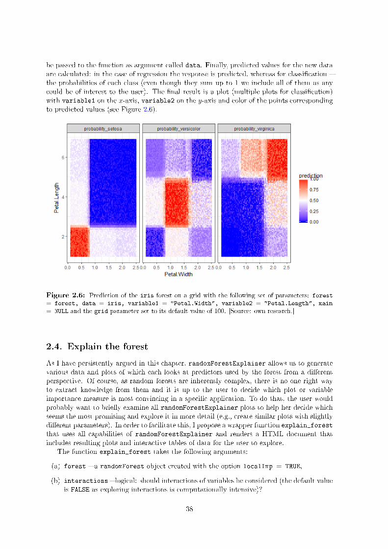
be passed to the function as argument called data. Finally, predicted values for the new dataare calculated: in the case of regression the response is predicted, whereas for classication the probabilities of each class (even though they sum up to 1 we include all of them as anycould be of interest to the user). The nal result is a plot (multiple plots for classication)with variable1 on the x-axis, variable2 on the y-axis and color of the points correspondingto predicted values (see Figure 2.6).

Figure 2.6: Prediction of the iris forest on a grid with the following set of parameters: forest

= forest, data = iris, variable1 = "Petal.Width", variable2 = "Petal.Length", main

= NULL and the grid parameter set to its default value of 100. [Source: own research.]

2.4. Explain the forest

As I have persistently argued in this chapter, randomForestExplainer allows us to generatevarious data and plots of which each looks at predictors used by the forest from a dierentperspective. Of course, as random forests are inherently complex, there is no one right wayto extract knowledge from them and it is up to the user to decide which plot or variableimportance measure is most convincing in a specic application. To do that, the user wouldprobably want to briey examine all randomForestExplainer plots to help her decide whichseems the most promising and explore it in more detail (e.g., create similar plots with slightlydierent parameters). In order to facilitate this, I propose a wrapper function explain_forestthat uses all capabilities of randomForestExplainer and renders a HTML document thatincludes resulting plots and interactive tables of data for the user to explore.

The function explain_forest takes the following arguments:

(a) forest a randomForest object created with the option localImp = TRUE,

(b) interactions logical: should interactions of variables be considered (the default valueis FALSE as exploring interactions is computationally intensive)?

38

(c) data the data frame on which forest was trained,

(d) vars a vector of names of predictors with respect to which interactions should beconsidered; if equal to NULL a default of at most 15 conditioning variables will be selectedusing the function important_variables,

(e) no_of_pred_plots the number of most frequent interactions of numeric variables forwhich prediction on a grid will be plotted, the default is 3,

(f) measures a vector of names of importance measures to be plotted by functionsplot_importance_ggpairs and plot_importance_rankings, by default the followingare used: mean minimal depth, number of nodes, number of trees in which the variablesplits the root and both measures calculated by the randomForest package.

Note that parameters (c)-(e) are redundant if interactions = FALSE as they are needed onlyby functions dedicated for analyzing interactions of variables. The default values of parametersallow the user to get the HTML report simply by passing the forest to the function. If onewants interactions to be considered as well, then apart from setting interactions to TRUE

the argument data needs to be specied.The function explain_forest is very simple: it creates a new environment to which it

passes the values of all parameters and uses rmarkdown::render to produce the HTML reportusing a template from the package directory with objects from the new environment. Thereport is saved to the working directory in a le called Your_forest_explained.html.

Clearly, the crucial element in rendering the document is the R markdown template thatis used. The template starts by listing the details of the forest (i.e., the formula used, thenumber of trees, the parameter r and information on prediction accuracy). Then, data forplotting are generated using functions min_depth_distribution, measure_importance andmin_depth_interactions if interactions are to be considered. Further, the distribution ofminimal depth is plotted and an interactive table with all importance measures is generatedfollowed by two multi-way importance plots: the rst contains structure measures (meanminimal depth, number of nodes and number of trees in which the variable splits the root),the second contains the increase in node purity measure, decrease in prediction accuracy afterpermutation and the p-value. Finally, both plots comparing all measures pairwise appear:the rst uses raw measures and the second rankings.

A conditional part of the template is used only if interactions = TRUE. Then, mean con-ditional minimal depth is plotted for up to 30 most frequent interactions and an interactivetable containing the data concerning interactions is given. Finally, up to no_of_pred_plots

most frequent interactions of numerical variables are plotted with plot_predict_interaction.Apart from all the aforementioned plots and tables, the template contains brief comments thathelp understand the results. For example output of the function see Appendix B.

All in all, the randomForestExplainer is a useful tool for exploring the importance ofvariables in a random forest. In my opinion the emphasis on visualization is a major advantageof the package, as well as the wrapper function that allows the user to see all plots withoutgetting to know the details of how to create them. A list of functions of the package availableto the user together with arguments and their default values can be found in Appendix A.

39

Chapter 3

Application to The Cancer Genome

Atlas data

In this chapter we use randomForestExplainer to explore a random forest built on dataconcerning glioblastoma brain cancer, generated by the TCGA Research Network [18]. Theforest is meant to predict whether a patient survived one year after the diagnosis using dataon expression of various genes. This is a typical example of a problem with large p and smalln as the data set contains many more genes than patients.

3.1. The data and random forest

Our data come from the R package RTCGA [11] and contain observations for 125 patientsthat have been diagnosed with glioblastoma. There are 16118 columns in the data: death1y(1 if the patient died within a year from diagnosis, 0 otherwise), Cluster (subtype of thetumor), age (age in years at the time of diagnosis) and 16115 columns containing numericalmeasurements of gene expression (names of columns are those of corresponding genes). Ouraim is to build a random forest that predicts death1y and to single out genes whose expressiondrives the prediction.

Before we proceed, we have to clarify the term gene expression in order to understandwhat we are actually modelling. It is worth noting that the denition of a gene depends oncontext and in our analysis a gene is a place on the DNA. In cell cycle dierent places of DNAtranscribe with dierent speed and eciency. We treat the amount of transcripts that arerelated to a given place as a random variable. In a single experiment we have gene expressionwhich is its realization. [16].

Moreover, we need to resolve the issue of missing data before we start our analysis. Insection 1.3.2 we discussed three ways of dealing with missing data in random forests: imputingmissing values, creating a "missing value" category for factors and using surrogate splits.We do not apply any of these approaches here as we do not wish to somewhat arbitrarilyimpute data, all our missing values are numeric gene expressions and surrogate splits are verycomputationally intensive and thus not implemented in the randomForest package. Therefore,in order to use all of our 125 observations we simply discard the 1989 out of 16117 predictorsthat contain missing values, which still leaves a plethora of variables for our analysis.

Finally, we use the randomForest::randomForest function to train a forest of 10000 trees,with option localImp = TRUE and r = b

√14128c = 118 candidate variables for each split.

The reason for growing such a big forest is that we are interested in distinguishing importantpredictors in that case the more trees in a forest the better, as they create more opportunities

41

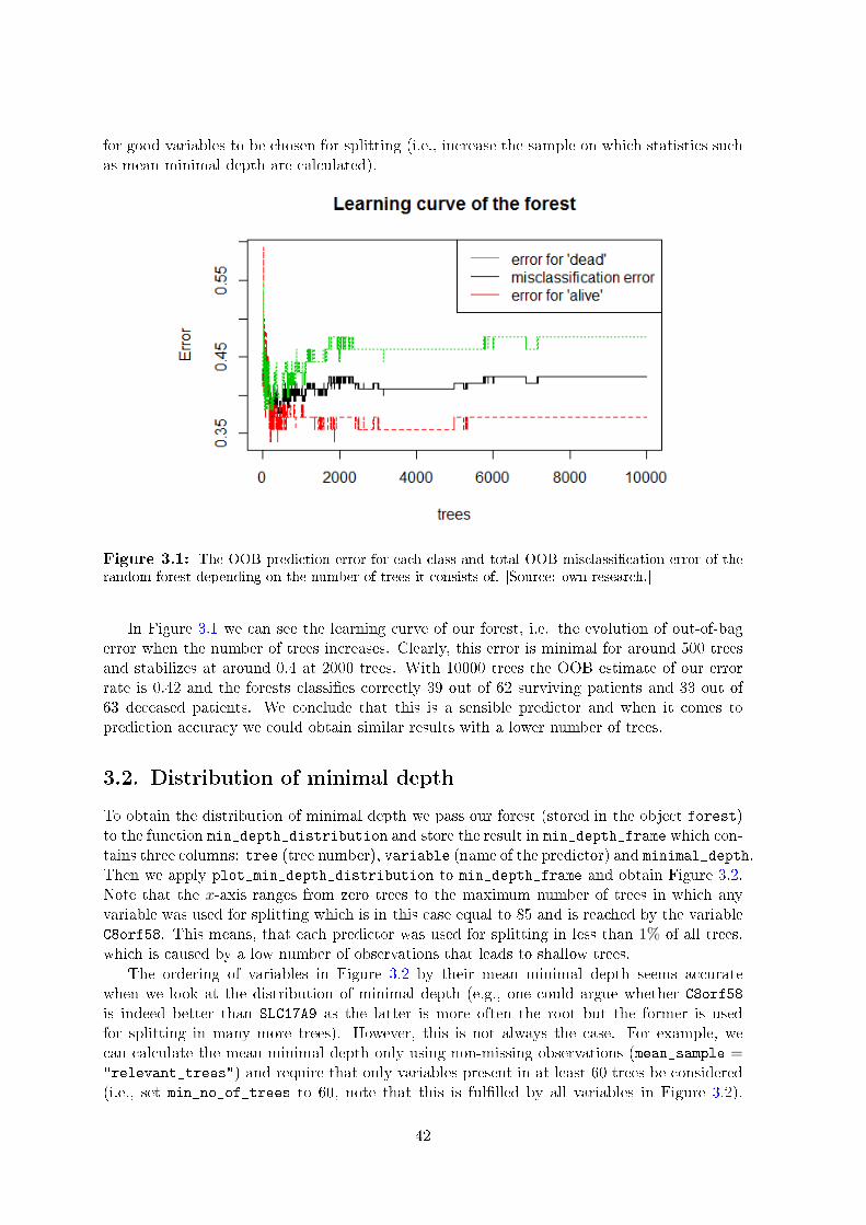
for good variables to be chosen for splitting (i.e., increase the sample on which statistics suchas mean minimal depth are calculated).

Figure 3.1: The OOB prediction error for each class and total OOB misclassication error of therandom forest depending on the number of trees it consists of. [Source: own research.]

In Figure 3.1 we can see the learning curve of our forest, i.e. the evolution of out-of-bagerror when the number of trees increases. Clearly, this error is minimal for around 500 treesand stabilizes at around 0.4 at 2000 trees. With 10000 trees the OOB estimate of our errorrate is 0.42 and the forests classies correctly 39 out of 62 surviving patients and 33 out of63 deceased patients. We conclude that this is a sensible predictor and when it comes toprediction accuracy we could obtain similar results with a lower number of trees.

3.2. Distribution of minimal depth

To obtain the distribution of minimal depth we pass our forest (stored in the object forest)to the function min_depth_distribution and store the result in min_depth_frame which con-tains three columns: tree (tree number), variable (name of the predictor) and minimal_depth.Then we apply plot_min_depth_distribution to min_depth_frame and obtain Figure 3.2.Note that the x-axis ranges from zero trees to the maximum number of trees in which anyvariable was used for splitting which is in this case equal to 85 and is reached by the variableC8orf58. This means, that each predictor was used for splitting in less than 1% of all trees,which is caused by a low number of observations that leads to shallow trees.

The ordering of variables in Figure 3.2 by their mean minimal depth seems accuratewhen we look at the distribution of minimal depth (e.g., one could argue whether C8orf58is indeed better than SLC17A9 as the latter is more often the root but the former is usedfor splitting in many more trees). However, this is not always the case. For example, wecan calculate the mean minimal depth only using non-missing observations (mean_sample ="relevant_trees") and require that only variables present in at least 60 trees be considered(i.e., set min_no_of_trees to 60, note that this is fullled by all variables in Figure 3.2).

42

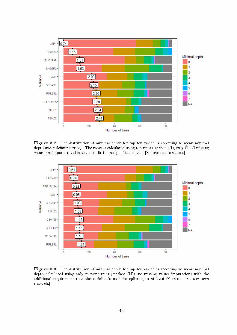
Figure 3.2: The distribution of minimal depth for top ten variables according to mean minimaldepth under default settings. The mean is calculated using top trees (method (II), only B−B missingvalues are imputed) and is scaled to t the range of the x-axis. [Source: own research.]

Figure 3.3: The distribution of minimal depth for top ten variables according to mean minimaldepth calculated using only relevant trees (method (III), no missing values imputation) with theadditional requirement that the variable is used for splitting in at least 60 trees. [Source: ownresearch.]

43

Some form of the last requirement is in this case necessary to avoid selecting variables thathave been by chance used for splitting once at the root. These settings result in Figure 3.3.

Clearly, method (III) of calculating mean minimal depth does not penalize missing ob-servations (when a variable is not used for splitting in a tree) and the plotting function onlyrequires the threshold of 60 trees to be fullled. This approach leads to the variable PPP1R12Aappearing as third best even though it is not only present in about 25% less trees than C8orf58

but also much less often splits the root node. C8orf58 on the other hand has minimal depthof 5 in some trees and this contributes to higher mean minimal depth in our opinion beingused for splitting at depth 5 in a tree is better than not being used at all.

Regardless of the exact parameters used in plot_min_depth_distribution, looking atthe whole distribution of minimal depth oers a lot more insight into the role that a predictorplays in a forest in contrast to looking only at the mean, especially as it can be calculated inmore than one way.

3.3. Various variable importance measures

To further explore variable importance measures we pass our forest to measure_importance

function and save the result as importance_frame it contains 14128 rows, each correspondingto a predictor, and 8 columns of which one stores the variable names and the rest store thevariable importance measures. Although this data frame can be useful in itself, we simplypass it to randomForestExplainer plotting functions.

In Figure 3.4 we present the result of plot_multi_way_importance for the default valuesof x_measure and y_measure, where the size of points reects the number of nodes split onthe variable (size_measure = "no_of_nodes"). In order not to obscure the picture with toomany points we only plot those that correspond to variables used for splitting at least in 30trees (min_no_of_trees = 30); in our case this requirement restricts the sample to 145 out of14128 observations. By default no_of_labels = 10 top variables in the plot are highlightedin blue and labeled these are selected using the function important_variables, i.e. usingthe sum of rankings based on importance measures used in the plot (more variables may belabeled if ties occur, as is the case here: 11 variables are highlighted).

Observe the marked negative relation between times_a_root and mean_min_depth inFigure 3.4 (though it looks linear it is not as the y-axis uses the square root scale). It isnecessary to remember that the plot excludes the worst predictors and including them couldmake the aforementioned relation look a lot dierent. However, if we are interested in therelation of the depicted importance measures only among variables that were used for splittingin at least 30 trees then our observation remains valid and we can conclude that using eitherof those two importance measures is sucient as they are highly (negatively) correlated.

In Figure 3.5 we present the multi-way importance plot for a dierent set of importancemeasures: decrease in predictive accuracy after permutation (x-axis), decrease in the Giniindex (y-axis) and levels of signicance (color of points). As in the previous plot, the twomeasures used as coordinates are strongly correlated, but in this case this is somewhat moresurprising as one is connected to the structure of the forest and the other to its prediction,whereas in the previous plot both measures reected the structure. Also, Figure 3.5 includesall 14128 observations and we can see that the most pronounced dierences appear amongtop variables. Moreover, the p-value criterion is evidently not very selective indeed, 1015predictors are signicant at the 1% signicance level. Interestingly, all 10 top variables inFigure 3.5 are also top variables in Figure 3.4 so we can be fairly condent that they are trulycrucial to predictive ability of our forest.

44

Figure 3.4: Multi-way importance plot for variables that were used for splitting in at least 30 trees.The x and y-axis measure mean minimal depth and number of splits at root of a variable and the sizeof points corresponds to the total number of nodes split on that variable. [Source: own research.]

Figure 3.5: Multi-way importance plot for all variables. The x and y-axis measure decrease inaccuracy when the variable is permuted and decrease in the Gini measure of node impurity resultingfrom splits on the variable, respectively. The color corresponds to variable signicance which is derivedfrom the number of nodes that split on it. [Source: own research.]

45

Generally, the multi-way importance plot oers a wide variety of possibilities so it canbe hard to select the most informative one. One idea of overcoming this obstacle is to rstexplore relations between dierent importance measures to then select three that least agreewith each other and use them in the multi-way importance plot to select top variables. Therst is easily done by plotting selected importance measures pairwise against each other usingplot_importance_ggpairs as in Figure 3.6. One could of course include all seven measuresin the plot but by default p-value and the number of trees are excluded as both carry similarinformation as the number of nodes.

In Figure 3.6 we can see that all depicted measures are highly correlated (of coursethe correlation of any measure with mean minimal depth is negative as the latter is low-est for best variables), but some less than others. Notably, the points in plots includingaccuracy_decrease and times_a_root are most dispersed, so these may be the measuresone should select. Moreover, regardless of which measures we compare, there is always onlya handful of points that stand out.

Figure 3.6: Pairwise comparison of ve importance measures: below the diagonal each pair ofmeasures is plotted against each other, pairwise correlation coecients are given above the diagonaland density estimates are depicted on the diagonal. [Source: own research.]

In addition to scatter plots and correlation coecients, Figure 3.6 also depicts densityestimate for each importance measure all of which are in this case very skewed. An attemptto eliminate this feature by plotting rankings instead of raw measures is implemented in thefunction plot_importance_rankings whose result is presented in Figure 3.7.

Density estimates in Figure 3.7 show that skewness was eliminated only for two out ofve importance measures: accuracy_decrease and gini_decrease. The skewness of rankingdistributions for other measures is most likely caused by frequent ties: e.g. 10370 predictors

46

were ranked last according to the times_a_root measure, as they were never used for splittingat the root. In general, ties are much less frequent for importance measures computed by therandomForest package also because they are measured on a continuous scale in contrast tothe discrete one used for root, node and tree counts.

When comparing the rankings in Figure 3.7 we can see that for accuracy_decrease andgini_decrease they more or less agree for observations with low ranks according to thosemeasures but strongly disagree for variables ranked higher according to accuracy_decrease.Also, observe that times_a_root and no_of_nodes dierentiate much more between variableswith low ranks than rankings according to other measures.

Figure 3.7: Pairwise comparison of rankings according to ve importance measures: below thediagonal each pair of rankings is plotted against each other, pairwise correlation coecients for rank-ings are given above the diagonal and density estimates are depicted on the diagonal. [Source: ownresearch.]

3.4. Variable interactions

After selecting a set of most important variables we can investigate interactions with respectto them, i.e. splits appearing in maximal subtrees with respect to one of the variables selected.To extract the names of 20 most important variables according to both the mean minimaldepth and number of trees in which a variable appeared, we pass our importance_frame tothe function important_variables with parameter k = 20 and selected importance measurespassed to the argument measures. After using the resulting vector of predictor names togetherwith the forest as arguments of min_depth_interactions we obtain a data frame containingthe mean conditional minimal depth for each interaction, its number of occurrences and the

47

unconditional mean minimal depth of the second variable in the interaction (for both typesof mean minimal depth we use the "top_trees" option).

Unfortunately, as we have many predictors and little observations, the trees in our forestare shallow and interactions are rare. Specically, only two interactions appeared 3 times, 153 two times and 7767 only one time. Thus, the mean conditional minimal depth is in this casemeaningless, as it is calculated on up to three observations. We conclude, that to properlyanalyze interactions we need to grow another random forest with either increased number oftrees or increased r (mtry) parameter so that more candidate variables will be tried at eachsplit.

We choose to grow a new forest with r = bp/3c = 4709 (this is the default r for regression)and after repeating the above calculations we save the result of min_depth_interactions asinteractions_frame. In the new forest 16 of the interactions considered appeared at least10 times in the forest, of which the most frequent, SLC17A9:IFIT2 (this corresponds to splitson IFIT2 in maximal subtrees of SLC17A9), a total of 29 times, which is a lot better thanbefore and oers some ground for interaction analysis.

Figure 3.8: 30 most frequent interactions ordered by decreasing frequency. The bars report meanconditional minimal depth and the points the unconditional mean minimal depth for the secondvariable in the interaction. Both are calculated using method (II) (mean_sample = "top_trees anduncond_mean_sample = "top_trees). [Source: own research.]

In Figure 3.8 we present the result of passing our interactions_frame to the functionplot_min_depth_interactions with the default number of most frequent interactions plotted(k = 30). An interesting thing about the interactions depicted is that they usually do notinclude top 20 predictors used as conditioning variables as the non-conditioning variable (only8 out of 30 do), which suggests that variables that are important in maximal subtrees withrespect to top predictors are not important in whole trees. This is actually what we wouldexpect from an interaction: some variable is only important conditional on another one andthis in most pronounced in the case of SLC17A9:IFIT2, as IFIT2 has mean minimal depthover 3.5 but in maximal subtrees of SLC17A9 it is often used for splitting immediately after

48

the root.Note that in Figure 3.8 the most frequent interaction has a lot lower mean conditional

minimal depth than the rest this is due to calculating the mean using method (II) thatpenalizes interactions that occur less frequently than the most frequent one. Of course, one canswitch between methods (I), (II) and (III) of calculating the mean both of the conditional andunconditional minimal depth but each of them has its drawbacks as discussed in section 2.1.2and we favour method (II). However, as plot_min_depth_interactions plots interactions bydecreasing frequency the major drawback of calculating the mean only for relevant variablesvanishes as interactions appearing only once but with conditional depth 0 will not be includedin the plot anyway. Thus, we repeat the computation of means using method (III) and reportthe result in Figure 3.9.

Figure 3.9: 30 most frequent interactions ordered by decreasing frequency. The bars report meanconditional minimal depth and the points the unconditional mean minimal depth for the secondvariable in the interaction. Both are calculated using method (III) (mean_sample = "relevant_trees

and uncond_mean_sample = "relevant_trees). [Source: own research.]

In Figure 3.9 we see, that all interactions have mean conditional minimal depth lower than1 meaning that the split on second variable in the interaction is often the daughter of the root,which is by denition split on the rst variable. This is not surprising as trees in our forestare shallow and there are not many possibilities for splits deep in maximal subtrees. Fromthis plot we can also infer that, apart from the rst one, the fourth, fth and sixth interactionseem important, with mean close to zero and number of occurrences equal to 16, 15 and 13,respectively.

To further investigate the interactions mentioned above (SLC17A9:IFIT2, LSP1:SH3BP2,SLC17A9:NRXN3 and NEIL1:HSPA1L) we use the function plot_predict_interaction to plotprediction of our forest on a grid of values for the components of each interaction. Unfortu-nately, neither of the plots oers any insight into how simultaneous changes of both variablesin the interaction shape the prediction. We report the plot for SLC17A9:IFIT2 in Figure 3.10as an example the other three look similar.

49

Figure 3.10: Prediction of the forest on a 100× 100 grid of values of variables SLC17A9 and IFIT2.The range of both axes corresponds to the ranges of the respective variables in our data set. [Source:own research.]

Clearly, higher values of SLC17A9 lead to higher predicted probabilities of the patientdying within a year from diagnosis, but this eect does not change with the variable IFIT2.All things considered, this is not surprising interaction of these two variables appears inonly 29 out of 10000 trees in our forest so it cannot inuence the prediction much. This is,as is frequency of interactions, a consequence of the structure of our high-p-low-n problem.We already modied our forest to be able to consider interactions at all, and we would haveto do more in order to investigate their eect on forest prediction. A possible solution wouldbe to build a forest using only a subset of our predictors, for example 50 top ones and allcomponents of interactions that appeared at least ve times in the forest.

3.5. Explain the forest

Instead of producing each plot separately, exploring the details of how each of them is madeand what parameters need to be specied, we could have just passed out data, forest andinteractions = TRUE to the function explain_forest. As in our analysis we mostly reliedon default values of parameters, so using the wrapper function would produce an HTMLdocument with all of the plots we discussed except Figure 3.3 and 3.9 as they were duplicateswith slightly changed parameters. Moreover, the resulting HTML document would containinteractive versions of both importance_frame and interactions_frame so that the usercould sort variables and interactions according to dierent importance measures or easily ndinformation concerning predictors of interest.

As we do not want to duplicate our results, we do not report the document producedby explain_forest for our forest. However, in Appendix B we include such documents fortwo other data sets. The rst concerns breast cancer and the problem there is to classify the

50

observations into one of ve groups corresponding to cancer subtypes on the basis of gene ex-pression data. The second data set contains information on students and their performance onthe PISA cognitive test. We build a forest that predicts the quantitative score in mathematicsof the students based on their various characteristics. Obviously, we modied somewhat theHTML documents obtained with the function explain_forest in order to t the format ofour paper. Notably, instead of interactive tables we show snippets of their non-interactivecounterparts and move them to the beginning of the document to take less space.

51

Summary

As I have shown throughout this thesis, random forests, though inherently complex, allow forat least two approaches of knowledge extraction: rst, one can analyze how the predictionof the forest changes after various modications of the data (e.g., inputs permutation) andsecond, one can come up with a number of useful summary statistics concerning the structureof a single tree and then aggregate them over the whole forest.

In particular, I have thoroughly discussed the minimal depth statistic and various waysof calculating its mean, each substantially dierent if the forest consists of shallow trees andvariables are often not used for splitting in a tree at all. Such considerations lead me tobelieve that it may be useful to investigate the whole distribution of minimal depth in theforest instead of just looking at its mean.

To address this and other issues I provide new ways of visualizing a random forest in R byintroducing the randomForestExplainer package that calculates various statistics measuringthe importance of variables and their interactions in a forest. Although the package mainlyutilizes existing variable importance measures with a few simple extensions, it possesses awide variety of graphical capabilities, all based on the ggplot2 package. Out of 11 functionsof the new package, six produce plots of which each presents predictors used in the forest froma dierent point of view. In my opinion, this focus on visualization is the main advantage ofthe new package.

Furthermore, the agship function explain_forest gives the user immediate insight intothe results that can be obtained by the package for a given forest without almost any need ofgetting to know how the package works. The resulting HTML document presents the resultsof all plotting functions of randomForestExplainer in turn, under default settings, allowingthe user to immediately asses the usefulness of each of them in the particular application.

When it comes to the example of predicting if the patient will survive one year fromdiagnosis of glioblastoma cancer, I found that out of a multitude of variables measuring geneexpression only a small group seems driving the prediction of the forest. Moreover, this ndingis consistent across plots using dierent variable importance measures for comparison. Myanalysis also helps in distinguishing which predictors are almost entirely useless when it comesto predicting the outcome so an analysis excluding them could be performed.

All in all, I believe that the ideas presented in this thesis can potentially help explainpredictions given by random forests. In other words, randomForestExplainer will hopefullylighten the random forest black box so that it will be of some more accessible shade of grey.

53

Appendix A

List of functions available in

randomForestExplainer

Below we list all functions available in the package randomForestExplainer. For each func-tion we include all its parameters and their default values, if any, and explain the nature ofobjects that have to be passed to the function as parameters that have no default value:

(1) min_depth_distribution(forest) the only argument is a randomForest object,

(2) plot_min_depth_distribution(min_depth_frame, k = 10, min_no_of_trees = 0,

mean_sample = "top_trees", mean_scale = FALSE, mean_round = 2, main ="Distribution of minimal depth and its mean") the rst argument is a result offunction (1),

(3) measure_importance(forest, mean_sample = "top_trees") the rst argument isa randomForest object grown with option localImp = TRUE,

(4) important_variables(importance_frame, k = 15, measures = names(importance

_frame)[2:5], ties_action = "all") the rst argument is a result of function (3),

(5) plot_multi_way_importance(importance_frame, x_measure = "mean_min_depth",

y_measure = "times_a_root", size_measure = NULL, min_no_of_trees = 0,

no_of_labels = 10, main = "Multi-way importance plot") the rst argumentis a result of function (3),

(6) plot_importance_ggpairs(importance_frame, measures = names(importance_

frame)[c(2, 4, 5, 3, 7)], main = "Relations between measures of importance")

the rst argument is a result of function (3),

(7) plot_importance_rankings(importance_frame, measures = names(importance_

frame)[c(2, 4, 5, 3, 7)], main = "Relations between rankings according to

different measures") the rst argument is a result of function (3),

(8) min_depth_interactions(forest, vars, mean_sample = "top_trees", uncond_

mean_sample = mean_sample) the rst argument is a randomForest object, the sec-ond one is a vector of names of (possibly all) predictors,

(9) plot_min_depth_interactions(interactions_frame, k = 30, main = paste0(

"Mean minimal depth for ", paste0(k, " most frequent interactions"))) therst argument is a result of function (8),

55

(10) plot_predict_interaction(forest, data, variable1, variable2, grid = 100,

main = paste0("Prediction of the forest for different values of ", paste0(

variable1, paste0(" and ", variable2)))) the rst argument is a randomForest

object, the second one is a data frame on which forest was trained, two subsequentones are names of predictors,

(11) explain_forest(forest, interactions = FALSE, data = NULL, vars = NULL,

no_of_pred_plots = 3, pred_grid = 100, measures = if (forest$type =="classification") c("mean_min_depth", "accuracy_decrease", "gini_decrease",

"no_of_nodes", "times_a_root") else c("mean_min_depth", "mse_increase",

"node_purity_increase", "no_of_nodes", "times_a_root")) the rst argumentis a randomForest object.

56

Appendix B

Additional examples

In this appendix we present documents produced by the randomForestExplainer functionexplain_forest applied to random forests grown on two dierent data sets.

B.1. Multi-label classication: breast cancer data

The rst data set comes from The Cancer Genome Atlas Project [18] and contains observationson 100 patients that have been diagnosed with breast cancer. We build a random forest thataims at predicting the subtype of cancer (one of ve: Basal, Her2, LumA, LumB or Normal)using 730 predictors containing numerical gene expression. Thus, this problem is similar toour glioblastoma example presented in Chapter 3 as it is also a classication problem withmany more predictors than observations leading to a forest with shallow trees.

We report the document produced by randomForestExplainer on pages 5862.

B.2. Regression: PISA data

The second data set comes from the PISA2012lite package and is a subset of the PISA 2012OECD database which contains information on students' performance on various cognitivetests and their personal characteristics. We use a relatively small sample that contains 12473observations on students from four members of the Visegrad Group (i.e., Czech Republic,Hungary, Poland and Slovak Republic). We build a random forest that aims at predicting thequantitative score in mathematics PV1MATH using 12 characteristics of a student such as hergender or index of wealth of her family. Clearly, this is a typical regression problem with nconsiderably bigger than p.

We report the document produced by randomForestExplainer on pages 6367.

57

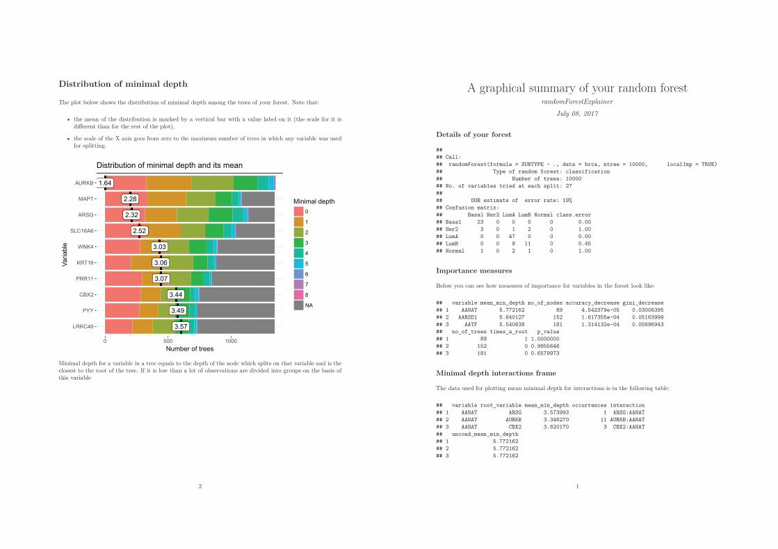
A graphical summary of your random forestrandomForestExplainer

July 08, 2017

Details of your forest

##

## Call:

## randomForest(formula = SUBTYPE ~ ., data = brca, ntree = 10000, localImp = TRUE)

## Type of random forest: classification

## Number of trees: 10000

## No. of variables tried at each split: 27

##

## OOB estimate of error rate: 19%

## Confusion matrix:

## Basal Her2 LumA LumB Normal class.error

## Basal 23 0 0 0 0 0.00

## Her2 3 0 1 2 0 1.00

## LumA 0 0 47 0 0 0.00

## LumB 0 0 9 11 0 0.45

## Normal 1 0 2 1 0 1.00

Importance measures

Below you can see how measures of importance for variables in the forest look like:

## variable mean_min_depth no_of_nodes accuracy_decrease gini_decrease

## 1 AANAT 5.772162 89 4.542379e-05 0.03006395

## 2 AARSD1 5.640127 152 1.617355e-04 0.05163999

## 3 AATF 5.540638 181 1.314132e-04 0.05696943

## no_of_trees times_a_root p_value

## 1 89 1 1.0000000

## 2 152 0 0.9955646

## 3 181 0 0.6579973

Minimal depth interactions frame

The data used for plotting mean minimal depth for interactions is in the following table:

## variable root_variable mean_min_depth occurrences interaction

## 1 AANAT ARSG 3.573993 1 ARSG:AANAT

## 2 AANAT AURKB 3.346270 11 AURKB:AANAT

## 3 AANAT CBX2 3.820170 3 CBX2:AANAT

## uncond_mean_min_depth

## 1 5.772162

## 2 5.772162

## 3 5.772162

1

Distribution of minimal depth

The plot below shows the distribution of minimal depth among the trees of your forest. Note that:

• the mean of the distribution is marked by a vertical bar with a value label on it (the scale for it isdifferent than for the rest of the plot),

• the scale of the X axis goes from zero to the maximum number of trees in which any variable was usedfor splitting.

2.32

1.64

3.44

3.06

3.57

2.28

3.07

3.49

2.52

3.03

LRRC46

PYY

CBX2

PRR11

KRT16

WNK4

SLC16A6

ARSG

MAPT

AURKB

0 500 1000

Number of trees

Vari

able

Minimal depth

0

1

2

3

4

5

6

7

8

NA

Distribution of minimal depth and its mean

Minimal depth for a variable in a tree equals to the depth of the node which splits on that variable and is theclosest to the root of the tree. If it is low than a lot of observations are divided into groups on the basis ofthis variable

2

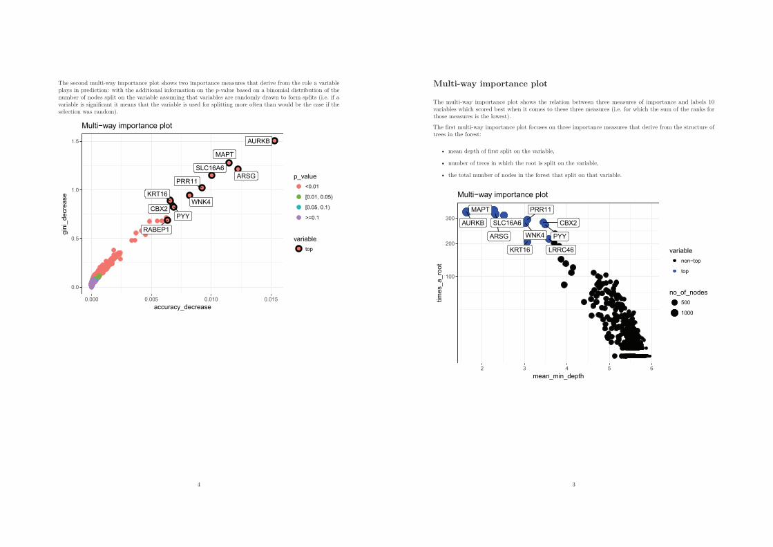
Multi-way importance plot

The multi-way importance plot shows the relation between three measures of importance and labels 10variables which scored best when it comes to these three measures (i.e. for which the sum of the ranks forthose measures is the lowest).

The first multi-way importance plot focuses on three importance measures that derive from the structure oftrees in the forest:

• mean depth of first split on the variable,

• number of trees in which the root is split on the variable,

• the total number of nodes in the forest that split on that variable.

ARSG

AURKB CBX2

KRT16 LRRC46

MAPT PRR11

PYY

SLC16A6

WNK4

100

200

300

2 3 4 5 6

mean_min_depth

tim

es_

a_

root

variable

non−top

top

no_of_nodes

500

1000

Multi−way importance plot

3

The second multi-way importance plot shows two importance measures that derive from the role a variableplays in prediction: with the additional information on the p-value based on a binomial distribution of thenumber of nodes split on the variable assuming that variables are randomly drawn to form splits (i.e. if avariable is significant it means that the variable is used for splitting more often than would be the case if theselection was random).

ARSG

AURKB

CBX2

KRT16

MAPT

PRR11

PYY

RABEP1

SLC16A6

WNK4

0.0

0.5

1.0

1.5

0.000 0.005 0.010 0.015

accuracy_decrease

gin

i_decre

ase

p_value

<0.01

[0.01, 0.05)

[0.05, 0.1)

>=0.1

variable

top

Multi−way importance plot

4

Compare importance measures

The plot below shows bilateral relations between the following importance measures: , if some variables arestrongly related to each other it may be worth to consider focusing only on one of them.

Corr:

−0.946

Corr:

−0.986

Corr:

0.983

Corr:

−0.994

Corr:

0.919

Corr:

0.967

Corr:

−0.924

Corr:

0.954

Corr:

0.96

Corr:

0.885

mean_min_depth accuracy_decrease gini_decrease no_of_nodes times_a_root

mean_

min

_depth

accura

cy_

decre

ase

gin

i_decre

ase

no_

of_

nodes

times_

a_

root

2 3 4 5 6 0.000 0.005 0.010 0.015 0.0 0.5 1.0 1.5 0 500 1000 0 100 200 300

0

1

2

0.000

0.005

0.010

0.015

0.0

0.5

1.0

1.5

0

500

1000

0

100

200

300

Relations between measures of importance

5

Compare rankings of variables

The plot below shows bilateral relations between the rankings of variables according to chosen importancemeasures. This approach might be useful as rankings are more evenly spread than corresponding importancemeasures. This may also more clearly show where the different measures of importance disagree or agree.

Corr:

0.896

Corr:

0.993

Corr:

0.914

Corr:

0.958

Corr:

0.867

Corr:

0.947

Corr:

0.635

Corr:

0.643

Corr:

0.643

Corr:

0.745

mean_min_depth accuracy_decrease gini_decrease no_of_nodes times_a_root

mean_

min

_depth

accura

cy_

decre

ase

gin

i_decre

ase

no_

of_

nodes

times_

a_

root

0 200 400 600 0 200 400 600 0 200 400 600 0 100 200 0 25 50 75

0e+00

5e−04

1e−03

0

200

400

600

0

200

400

600

0

100

200

0

25

50

75

Relations between rankings according to different measures

6

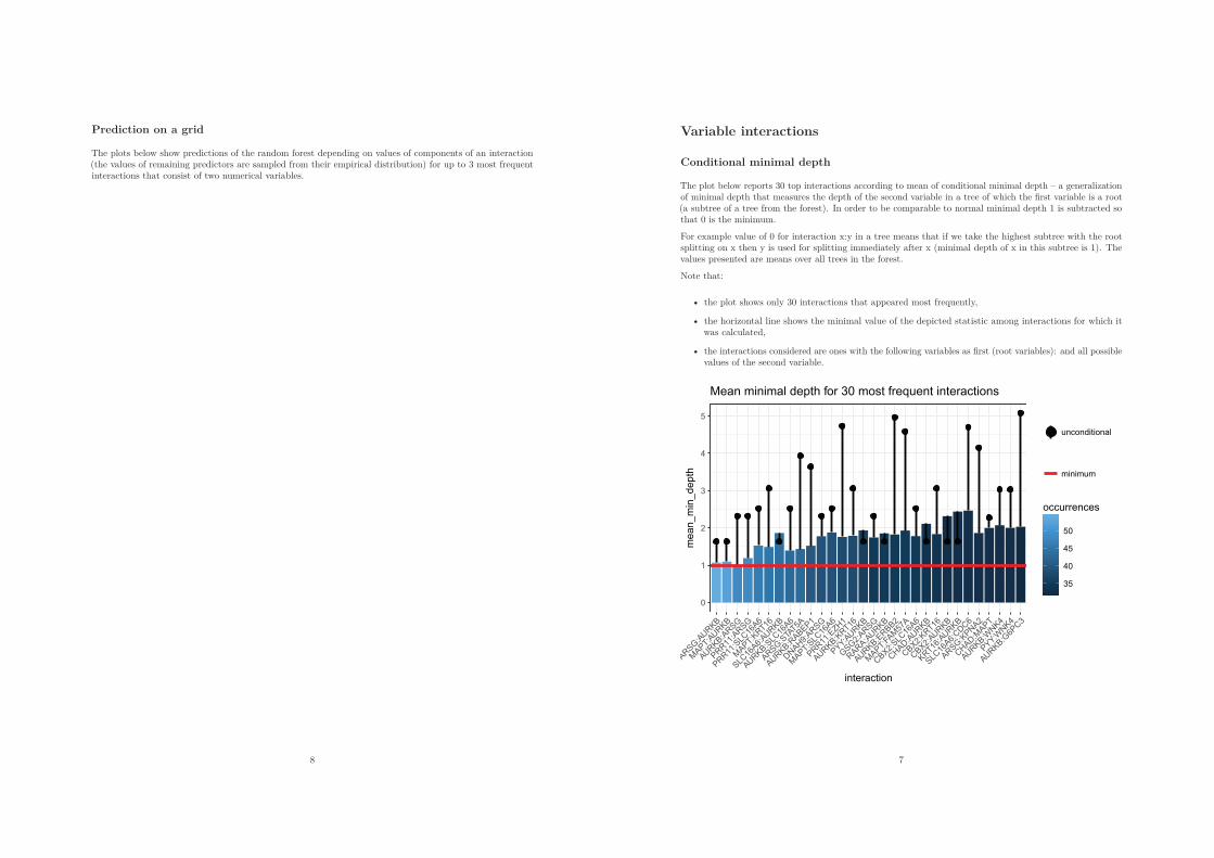
Variable interactions

Conditional minimal depth

The plot below reports 30 top interactions according to mean of conditional minimal depth – a generalizationof minimal depth that measures the depth of the second variable in a tree of which the first variable is a root(a subtree of a tree from the forest). In order to be comparable to normal minimal depth 1 is subtracted sothat 0 is the minimum.

For example value of 0 for interaction x:y in a tree means that if we take the highest subtree with the rootsplitting on x then y is used for splitting immediately after x (minimal depth of x in this subtree is 1). Thevalues presented are means over all trees in the forest.

Note that:

• the plot shows only 30 interactions that appeared most frequently,

• the horizontal line shows the minimal value of the depicted statistic among interactions for which itwas calculated,

• the interactions considered are ones with the following variables as first (root variables): and all possiblevalues of the second variable.

0

1

2

3

4

5

AR

SG

:AU

RK

B

MA

PT:A

UR

KB

AUR

KB

:AR

SG

PR

R11

:AR

SG

PR

R11

:SLC

16A

6

MA

PT:K

RT16

SLC

16A

6:AU

RK

B

AUR

KB

:SLC

16A

6

AR

SG

:STA

T5A

AUR

KB

:RA

BE

P1

DN

AH

9:A

RS

G

MA

PT:S

LC16

A6

PR

R11

:EZH

1

AUR

KB

:KR

T16

PY

Y:AU

RK

B

GS

G2:

AR

SG

RA

RA

:AU

RK

B

AUR

KB

:ER

BB

2

MA

PT:F

AM

57A

CB

X2:

SLC

16A

6

CH

AD

:AU

RK

B

CB

X2:

KR

T16

CB

X2:

AUR

KB

KR

T16:A

UR

KB

SLC

16A

6:C

DC

6

AR

SG

:KP

NA

2

CH

AD

:MA

PT

AUR

KB

:WN

K4

PY

Y:WN

K4

AUR

KB

:G6P

C3

interactionm

ean_

min

_depth

unconditional

minimum

35

40

45

50

occurrences

Mean minimal depth for 30 most frequent interactions

7

Prediction on a grid

The plots below show predictions of the random forest depending on values of components of an interaction(the values of remaining predictors are sampled from their empirical distribution) for up to 3 most frequentinteractions that consist of two numerical variables.

8

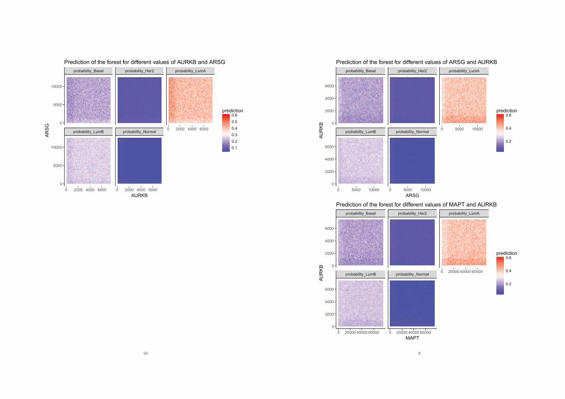
probability_LumB probability_Normal

probability_Basal probability_Her2 probability_LumA

0 5000 10000 0 5000 10000

0 5000 10000

0

2000

4000

6000

0

2000

4000

6000

ARSG

AU

RK

B

0.2

0.4

0.6prediction

Prediction of the forest for different values of ARSG and AURKB

probability_LumB probability_Normal

probability_Basal probability_Her2 probability_LumA

0 20000 40000 60000 0 20000 40000 60000

0 20000 40000 60000

0

2000

4000

6000

0

2000

4000

6000

MAPT

AU

RK

B

0.2

0.4

0.6prediction

Prediction of the forest for different values of MAPT and AURKB

9

probability_LumB probability_Normal

probability_Basal probability_Her2 probability_LumA

0 2000 4000 6000 0 2000 4000 6000

0 2000 4000 6000

0

5000

10000

0

5000

10000

AURKB

AR

SG

0.1

0.2

0.3

0.4

0.5

0.6prediction

Prediction of the forest for different values of AURKB and ARSG

10

A graphical summary of your random forestrandomForestExplainer

July 08, 2017

Details of your forest

##

## Call:

## randomForest(formula = PV1MATH ~ ., data = pisa, localImp = TRUE)

## Type of random forest: regression

## Number of trees: 500

## No. of variables tried at each split: 4

##

## Mean of squared residuals: 7293.245

## % Var explained: 18.91

Importance measures

Below you can see how measures of importance for variables in the forest look like:

## variable mean_min_depth no_of_nodes mse_increase node_purity_increase no_of_trees times_a_root

## 1 CNT 1.414 62408 1477.227 5861251 500 109

## 2 ISCEDO 1.216 19526 1340.554 6915233 500 155

## 3 OECD NA 0 0.000 0 0 0

## p_value

## 1 1.472617e-51

## 2 1.000000e+00

## 3 1.000000e+00

Minimal depth interactions frame

The data used for plotting mean minimal depth for interactions is in the following table:

## variable root_variable mean_min_depth occurrences interaction uncond_mean_min_depth

## 1 CNT CNT 3.574100 485 CNT:CNT 1.414

## 2 CNT ISCEDO 1.892594 490 ISCEDO:CNT 1.414

## 3 CNT OECD NaN 0 OECD:CNT 1.414

1

Distribution of minimal depth

The plot below shows the distribution of minimal depth among the trees of your forest. Note that:

• the mean of the distribution is marked by a vertical bar with a value label on it (the scale for it isdifferent than for the rest of the plot),

• the scale of the X axis goes from zero to the maximum number of trees in which any variable was usedfor splitting.

1.41

1.22

3.36

2.34

2.95

2.29

3.23

2.36

2.67

1.66

ST04Q01

ST115Q01

ST08Q01

ST27Q02

ST27Q01

ST05Q01

ST09Q01

WEALTH

CNT

ISCEDO

0 100 200 300 400 500

Number of trees

Vari

able

Minimal depth

0

1

2

3

4

5

6

NA

Distribution of minimal depth and its mean

Minimal depth for a variable in a tree equals to the depth of the node which splits on that variable and is theclosest to the root of the tree. If it is low than a lot of observations are divided into groups on the basis ofthis variable

2

Multi-way importance plot

The multi-way importance plot shows the relation between three measures of importance and labels 10variables which scored best when it comes to these three measures (i.e. for which the sum of the ranks forthose measures is the lowest).

The first multi-way importance plot focuses on three importance measures that derive from the structure oftrees in the forest:

• mean depth of first split on the variable,

• number of trees in which the root is split on the variable,

• the total number of nodes in the forest that split on that variable.

CNT

ISCEDO

ST05Q01

ST08Q01

ST09Q01

ST115Q01

ST27Q01

ST27Q02

ST46Q04

WEALTH

40

80

120

160

2 3 4

mean_min_depth

tim

es_

a_

root

no_of_nodes

50000

100000

150000

variable

non−top

top

Multi−way importance plot

3

The second multi-way importance plot shows two importance measures that derive from the role a variableplays in prediction: with the additional information on the p-value based on a binomial distribution of thenumber of nodes split on the variable assuming that variables are randomly drawn to form splits (i.e. if avariable is significant it means that the variable is used for splitting more often than would be the case if theselection was random).

CNT

ISCEDO

ST04Q01

ST05Q01ST08Q01

ST09Q01ST27Q01

ST27Q02

ST46Q04

WEALTH

0

2500000

5000000

7500000

10000000

12500000

0 500 1000 1500

mse_increase

node_

puri

ty_

incre

ase variable

top

p_value

<0.01

>=0.1

Multi−way importance plot

4

Compare importance measures

The plot below shows bilateral relations between the following importance measures: , if some variables arestrongly related to each other it may be worth to consider focusing only on one of them.

Corr:

−0.801

Corr:

−0.659

Corr:

0.84

Corr:

−0.204

Corr:

0.441

Corr:

0.807

Corr:

−0.848

Corr:

0.823

Corr:

0.632

Corr:

0.093

mean_min_depth mse_increase node_purity_increase no_of_nodes times_a_root

mean_

min

_depth

mse_

incre

ase

node_

purity

_in

cre

ase

no_

of_

nodes

times_

a_

root

2 3 4 0 500 1000 1500 025000005000000750000010000000125000000 50000100000150000 0 50 100 150

0.0

0.1

0.2

0.3

0

500

1000

1500

0

2500000

5000000

7500000

10000000

12500000

0

50000

100000

150000

0

50

100

150

Relations between measures of importance

5

Compare rankings of variables

The plot below shows bilateral relations between the rankings of variables according to chosen importancemeasures. This approach might be useful as rankings are more evenly spread than corresponding importancemeasures. This may also more clearly show where the different measures of importance disagree or agree.

Corr:

0.846

Corr:

0.714

Corr:

0.923

Corr:

0.187

Corr:

0.511

Corr:

0.643

Corr:

0.939

Corr:

0.698

Corr:

0.58

Corr:

0.0196

mean_min_depth mse_increase node_purity_increase no_of_nodes times_a_root

mean_

min

_depth

mse_

incre

ase

node_

purity

_in

cre

ase

no_

of_

nodes

times_

a_

root

5 10 5 10 5 10 5 10 2.5 5.0 7.5 10.0

0.00

0.02

0.04

0.06

0.08

0

5

10

15

−5

0

5

10

15

20

0

5

10

15

20

0

5

10

Relations between rankings according to different measures

6

Variable interactions

Conditional minimal depth

The plot below reports 30 top interactions according to mean of conditional minimal depth – a generalizationof minimal depth that measures the depth of the second variable in a tree of which the first variable is a root(a subtree of a tree from the forest). In order to be comparable to normal minimal depth 1 is subtracted sothat 0 is the minimum.

For example value of 0 for interaction x:y in a tree means that if we take the highest subtree with the rootsplitting on x then y is used for splitting immediately after x (minimal depth of x in this subtree is 1). Thevalues presented are means over all trees in the forest.

Note that:

• the plot shows only 30 interactions that appeared most frequently,

• the horizontal line shows the minimal value of the depicted statistic among interactions for which itwas calculated,

• the interactions considered are ones with the following variables as first (root variables): and all possiblevalues of the second variable.

0

1

2

3

CN

T:ST46

Q04

ISC

ED

O:W

EA

LTH

CN

T:WE

ALT

H

ISC

ED

O:S

T27Q

02

WE

ALT

H:W

EA

LTH

CN

T:ST27

Q02

ST05

Q01

:WE

ALT

H

ISC

ED

O:C

NT

ISC

ED

O:S

T04Q

01

ST05

Q01

:ST27

Q02

ISC

ED

O:S

T46Q

04

ST05

Q01

:ST46

Q04

ISC

ED

O:S

T08Q

01

WE

ALT

H:S

T46Q

04

ST09

Q01

:WE

ALT

H

CN

T:CN

T

WE

ALT

H:S

T27Q

02

ISC

ED

O:S

T115Q

01

ST27

Q01

:WE

ALT

H

ST27

Q02

:WE

ALT

H

CN

T:ST08

Q01

WE

ALT

H:S

T08Q

01

ST09

Q01

:ST27

Q02

ST09

Q01

:ST46

Q04

CN

T:ST04

Q01

ST27

Q02

:ST46

Q04

CN

T:ST11

5Q01

ST05

Q01

:ST04

Q01

CN

T:ST09

Q01

ST27

Q01

:ST46

Q04

interactionm

ean_

min

_depth

unconditional

480

490

occurrences

minimum

Mean minimal depth for 30 most frequent interactions

7

Prediction on a grid

The plots below show predictions of the random forest depending on values of components of an interaction(the values of remaining predictors are sampled from their empirical distribution) for up to 3 most frequentinteractions that consist of two numerical variables.

8

1

2

3

4

−4 −2 0 2

WEALTH

ST

115Q

01

350

400

450

500

550

600

prediction

Prediction of the forest for different values of WEALTH and ST115Q01

−4

−2

0

2

1 2 3 4

ST115Q01

WE

ALT

H

400

500

600

prediction

Prediction of the forest for different values of ST115Q01 and WEALTH

9

List of Figures

1.1. Illustration of linked brushing for the iris data . . . . . . . . . . . . . . . . . 111.2. The model-tting process of simulated annealing with 20 random starts . . . 131.3. Decision tree and decision regions for a classication problem on the iris data 141.4. Illustration of the concept of maximal subtrees . . . . . . . . . . . . . . . . . 20

2.1. The iris forest: minimal depth distribution . . . . . . . . . . . . . . . . . . . 282.2. The iris forest: multi-way importance plot . . . . . . . . . . . . . . . . . . . 312.3. The iris forest: pairwise plots of importance measures . . . . . . . . . . . . . 322.4. The iris forest: pairwise plots of rankings of importance . . . . . . . . . . . 332.5. The iris forest: mean conditional minimal depth . . . . . . . . . . . . . . . . 372.6. The iris forest: prediction on a grid . . . . . . . . . . . . . . . . . . . . . . . 38

3.1. The learning curve of our random forest . . . . . . . . . . . . . . . . . . . . . 423.2. Minimal depth distribution with mean for top trees . . . . . . . . . . . . . . . 433.3. Minimal depth distribution with mean for relevant trees . . . . . . . . . . . . 433.4. Multi-way importance plot: minimal depth, number of nodes, times a root . . 453.5. Multi-way importance plot: accuracy decrease, Gini decrease and p-value . . . 453.6. Pairwise comparison of ve importance measures . . . . . . . . . . . . . . . . 463.7. Pairwise comparison of rankings according to ve importance measures . . . . 473.8. Mean conditional minimal depth on top trees for best interactions . . . . . . . 483.9. Mean conditional minimal depth on relevant trees for best interactions . . . . 493.10. Prediction of the forest on a grid of values of SLC17A9 and IFIT2 . . . . . . . 50

69

List of Algorithms

2.1. Calculating depth of nodes in a single tree . . . . . . . . . . . . . . . . . . . . 242.2. Calculating minimal depth in every tree of a forest . . . . . . . . . . . . . . . 252.3. Count the trees in which each variable had a given minimal depth . . . . . . . 252.4. Calculate means of minimal depth in one of three ways . . . . . . . . . . . . . 262.5. Plot the distribution of minimal depth . . . . . . . . . . . . . . . . . . . . . . 282.6. Calculate variable importance measures . . . . . . . . . . . . . . . . . . . . . 302.7. Select k most important variables in a forest . . . . . . . . . . . . . . . . . . . 312.8. Calculating conditional depth of nodes in a single tree . . . . . . . . . . . . . 352.9. Calculating conditional minimal depth in a forest . . . . . . . . . . . . . . . . 352.10. Calculating means of conditional minimal depth in a forest . . . . . . . . . . . 36

71

Bibliography

[1] André Altmann, Laura Tolosi, Oliver Sander, and Thomas Lengauer. Permutation im-portance: a corrected feature importance measure. Bioinformatics, 26(10):13401347,2010.

[2] Leo Breiman. Random forests. Machine Learning, 45(1):532, 2001.

[3] Leo Breiman. Statistical modeling: The two cultures (with comments and a rejoinder bythe author). Statistical Science, 16(3):199231, 2001.

[4] Chao Chen, Andy Liaw, and Leo Breiman. Using random forest to learn imbalanceddata. Technical report, Department of Statistics, University of Berkeley, 2004.

[5] Trevor Hastie, Robert Tibshirani, and Jerome Friedman. The Elements of Statistical

Learning. Springer Series in Statistics. Springer New York Inc., New York, NY, USA,2016.

[6] Torsten Hothorn, Kurt Hornik, and Achim Zeileis. Unbiased recursive partitioning: Aconditional inference framework. Journal of Computational and Graphical Statistics,15(3):651674, 2006.

[7] Hemant Ishwaran. Variable importance in binary regression trees and forests. ElectronicJournal of Statistics, 1:519537, 2007.

[8] Hemant Ishwaran, Udaya B. Kogalur, Eiran Z. Gorodeski, Andy J. Minn, and Michael S.Lauer. High-dimensional variable selection for survival data. Journal of the American

Statistical Association, 105(489):205217, 2010.

[9] Hemant Ishwaran, Udaya B. Kogular, Eugene H. Blackstone, and Michael S. Lauer.Random survival forests. The Annals of Applied Statistics, 2(3):841860, 2008.

[10] Jacek Koronacki and Jan wik. Statystyczne systemy ucz¡ce si¦. Akademicka OcynaWydawnicza EXIT, Warszawa, 2nd edition, 2008.

[11] Marcin Kosi«ski and Przemysªaw Biecek. RTCGA: The cancer genome atlas data inte-gration. R package version 1.2.5, 2016.

[12] Andy Liaw and Matthew Wiener. Classication and Regression by randomForest. R

News, 2(3):1822, 2002.

[13] Marco Túlio Ribeiro, Sameer Singh, and Carlos Guestrin. "Why Should I Trust You?":Explaining the predictions of any classier. In KDD '16 Proceedings of the 22nd ACM

SIGKDD International Conference on Knowledge Discovery and Data Mining, pages11351144, 2016.

73

[14] Ivan Sanchez, Tim Rocktaschel, Sebastian Riedel, and Sameer Singh. Towards extract-ing faithful and descriptive representations of latent variable models. In AAAI Spring

Syposium on Knowledge Representation and Reasoning (KRR): Integrating Symbolic and

Neural Approaches, 2015.

[15] Galit Shmueli. To explain or to predict? Statistical Science, 25(3):289310, 2010.

[16] Katarzyna Sobiczewska. Analiza metod uczenia maszynowego wykorzystywanych w bu-dowaniu sygnatur genetycznych. Master's thesis, Politechnika Warszawska, 2016.

[17] Carolin Strobl, Anne-Laure Boulesteix, Achim Zeileis, and Torsten Hothorn. Bias inrandom forest variable importance measures: Illustrations, sources and a solution. BMC

Bioinformatics, 8(25):14712105, 2007.

[18] John Weinstein, Eric Collission, Gordon Mills, Kenna Mills Shaw, Brad Ozenberger, KyleEllrott, Ilya Shmulevich, Chris Sander, and Joshua Stuart. Cancer genome atlas researchnetwork. Nature Genetics, 45:11131120, 2013.

[19] Hadley Wickham, Dianne Cook, and Heike Hofmann. Visualizing statistical models:Removing the blindfold. Statistical Analysis and Data Mining, 8(4):203225, 2015.

74