Embed Size (px)
Citation preview

For multiple-author papers: Contact author designated by * Presenting author designated by underscore
Structural Stability Session Organizer: Herbert MANG (Technical University of Vienna) Plenary Lecture: Abstract, Slides and Video Answers to three not quite straightforward questions in structural stability Andreas STEINBOECK, Gerhard HOEFINGER, Xin JIA, Herbert A. MANG (Technical University of Vienna) Keynote Lecture Limit-point and postbuckling behavior of steel trusses under thermal and mechanical loadings Yeong Bin YANG*, T.J. LIN (National Taiwan University) Modeling thin-walled cold-formed steel members and systems Benjamin W. SCHAFER*, R. H. SANGREE, Cristopher MOEN, M. SEIF, Y. SHIFFERAW, V. ZEINODDINI, Z. J. LI, O. IUORIO, Y. GUAN (Johns Hopkins University) Multi parametrical instability of straight bars Jan B. OBREBSKI (Warsaw University of Technology) The effect of predetermined delaminations on buckling and post-buckling behavior of spatial composite timber beams and frames Miran SAJE*, Urban RODMAN, Dejan ZUPAN, Igor PLANINC (University of Ljubljana) Keynote Lecture Buckling and sensitivity analysis of imperfect shells involving contact Karl SCHWEIZERHOF*, Eduard EWERT (University of Karlsruhe) Keynote Lecture Determining the stability of tensegrities and generic global rigidity Robert CONNELLY (Cornell University) Initial imperfection identification in shell buckling problems Christopher J. STULL*, Christopher J. EARLS, Wilkins AQUINO (Cornell University) Buckling phenomena, analysis and design of axially compressed cylindrical shells with co-existent external pressure Werner GUGGENBERGER*, Medhanye B. TEKLEAB (TU Graz)

Proceedings of the 6th International Conference on
Computation of Shell and Spatial Structures
IASS-IACM 2008: “Spanning Nano to Mega”
28-31 May 2008, Cornell University, Ithaca, NY, USA
John F. ABEL and J. Robert COOKE (eds.)
1
Answers to three not quite straightforward questions in
structural stability
Andreas STEINBOECK, Gerhard HOEFINGER, Xin JIA, Herbert A. MANG*
*Institute for Mechanics of Materials and Structures, Vienna University of Technology
Karlsplatz 13/202, 1040 Vienna, Austria
Abstract
In this contribution, the following three questions will be answered by means of both, theoretical proofs and
practical examples:
• Are linear prebuckling paths and linear stability problems mutually conditional?
• Does the conversion from imperfection sensitivity into imperfection insensitivity by means of a
modification of the original structural design require a symmetric postbuckling path?
• Is hilltop buckling, characterized by the coincidence of a bifurcation point and a snap-through point on a
load-displacement path, necessarily imperfection sensitive?
1. Introduction
Despite the long history of structural stability as a field of great scientific relevance and practical importance, it
holds a number of questions which so far were not rigorously answered. The reasons for some pieces of the
structural stability landscape still being uncharted range from missing mathematical proofs to aspects that are
commonly regarded as matters of course, which, at first glance, render thorough proofs dispensable. This is the
motivation to ponder in this contribution over the three questions mentioned in the abstract.
They are related to the computation and study of load-displacement paths and, in particular, to loss of stability
phenomena, exhibiting either imperfection sensitivity or insensitivity (Mang et al. [4]). After a brief theoretical
introduction into the topic, theoretical answers to the posed questions will be given based on mathematical
proofs. The lecture will supplement the theory by representative problems which were solved analytically and
numerically, respectively.
2. Theoretical foundations
The behavior of a static, conservative system can be deduced from the potential energy function
( , ) : .× →ℝ ℝ ℝNV u λ The vector ∈ℝN
u contains the displacement coordinates, implying that the system has N
degrees of freedom. The parameter ∈ℝλ is a load multiplier scaling a constant reference load .∈ℝNP
Therefore, ,( , ) : ( )= = −IVu
G u F u Pλ λ may be interpreted as an out-of-balance force, which vanishes along any
equilibrium path in the u-λ-space. Here, ( )∈ℝI NF u is the vector of internal forces.
A crossing point ( , )C Cu λ of two equilibrium paths is called a bifurcation point. The equilibrium path
containing the unloaded state is the primary or prebuckling path ( ( ), ),ɶu λ λ the other one the secondary or
postbuckling path.
The differential of ,=G 0 i.e.,
,⋅ − =T d dK u P 0λ (1)

6th International Conference on Computation of Shell and Spatial Structures IASS-IACM 2008, Ithaca
2
with the symmetric tangent-stiffness matrix ,: ( , ),=T Vuu
K u λ commonly serves as the basis for the solution of
nonlinear structural problems by the FEM. Specializing (1) for the primary path, using the notation
,( ) : ( ( ), ),=ɶ ɶT V
uuK uλ λ λ and disregarding, for the time being, snap-through points characterized by 0,=dλ (1)
can be expressed as
, ,⋅ − =ɶ ɶTK u P 0λ (2)
or, after differentiation with respect to λ, as
, , , .⋅ + ⋅ =ɶ ɶɶ ɶT TK u K u 0λ λ λλ (3)
The secondary path is parameterized by a scalar ,η with 0=η corresponding to the bifurcation point ( , ).C Cu λ
The displacement offset between the primary and the secondary path is defined by the vector ( ) .∈ℝNv η Thus,
( ) ( ( )) ( )= +ɶu u vη λ η η describes the displacement along the secondary path. Single-valuedness is guaranteed
for ( ) : →ℝ ℝN
v η but not for ( ) : .→ɶ ℝ ℝN
u λ Frequently, the coordinates are chosen such that η is a
component of u. Insertion of the series expansions
2 3 41 2 3( ) ( )= + + + +OCλ η λ λη λ η λ η η (4)
2 3 41 2 3( ) ( )= + + +Ov v v vη η η η η (5)
into the specialization of G for the secondary path, i.e., ( ) ( ( ( )) ( ), ( )) ,= + =ɶG G u v 0η λ η η λ η yields the new
series expansion
2 30 1 2( ) ( ) 0C C Cη η η η= + + + =G G G G O (6)
with , 0| / ! .== ∀ ∈nnC n nG G ℕη η Since (6) must hold for arbitrary values of ,η .= ∀ ∈nC nG 0 ℕ This condition
paves the way for successive calculation of the unknowns 1 1 2 2, , , ,v vλ λ etc. To render this calculation unique,
the length of 1v has to be chosen (not equal to zero) and the orthogonality condition 1 0 1,⋅ = ∀ >i iv v suggested
in Budiansky [2] can be materialized.
3. Are linear prebuckling paths and linear stability problems mutually conditional?
A primary path is linear if
, const. .= = ∀ ∈ɶ ℝu kλ λ (7)
Thus, ( ) (0)= +ɶ ɶu u kλ λ with a constant (non-zero) vector k. A stability problem is considered as linear if the
tangent stiffness matrix specialized for the primary path can be written as
0 1,= +ɶTK K Kλ (8)
with constant matrices 0K and 1K (cf. Zienkiewicz and Taylor [7]). Provided that the unloaded state ( 0)=λ
is stable, 0K is positive definite. 1 1= TK K may be any constant non-zero matrix. Consequently,
det( ( )) 0,=ɶTK λ i.e., the condition for loss of stability, is a scalar algebraic equation in λ, which facilitates the
computation of the critical load level .Cλ
3.1 A linear prebuckling path is not sufficient for a linear stability problem
Utilization of (7) in (3) yields
, .⋅ = ∀ ∈ɶ ℝTK k 0λ λ (9)
Clearly, for any value of λ, k is a zero eigenvector of , .ɶTK λ Yet, this is not sufficient for (8), i.e. (7)⇒/ (8).
3.2 A linear stability problem is not sufficient for a linear prebuckling path
Substitution of (8) into (2) shows that for a linear stability problem, ɶu is defined by the differential equation
0 1 ,( ) .+ ⋅ − =ɶK K u P 0λλ (10)

6th International Conference on Computation of Shell and Spatial Structures IASS-IACM 2008, Ithaca
3
The existence of an appropriate vector k such that (7) is a solution of (10) is not guaranteed. Thus, (8)⇒/ (7),
which is explained in more detail in Steinboeck and Mang [6]. Moreover, it follows from (10) that a linear
stability problem entails a linear prebuckling path only if in addition 1 , .⋅ = ∀ɶK u 0λ λ
4. Does the conversion from imperfection sensitivity into imperfection insensitivity require a symmetric postbuckling path?
To achieve a conversion from imperfection sensitivity into insensitivity, the original structure must be modified.
The degree of such a modification may be parameterized by means of a scalar κ. In many cases, it is of interest
to find values of κ, for which the system is imperfection insensitive.
4.1 Conditions for symmetric load-displacement paths
For a definition of symmetric load-displacement paths, it is reasonable to start out from the potential energy
function. As suggested in Steinboeck et al. [5], symmetry requires
( , ) ( ( ), ) ( , ) ,= ∀ ∈ ×ℝ ℝNV Vu T u uλ λ λ (11)
where the linear mapping : →ℝ ℝN N
T is an element of a symmetry group. Moreover, symmetry of the
secondary path with respect to η requires
( ( ( )) ( ), ( )) ( ( ( )) ( ), ( )) .+ = − + − − ∀ ∈ɶ ɶ ℝV Vu v u vλ η η λ η λ η η λ η η (12)
Condition (11) must hold along the primary path, and the uniqueness of this path implies ( ) ( ( )).=ɶ ɶu T uλ λ
Moreover, a comparison of (11) and (12) reveals that ( ) ( )= −λ η λ η and ( ) ( ( )).= −v T vη η These conditions
may be summarized as follows:
A postbuckling path is said to be symmetrical with respect to η if it obeys the definition:
( ) ( )= − ∧λ η λ η (13)
( ) ( ( ))= − ∧v T vη η (14)
( ( )) ( ( ( ))).=ɶ ɶu T uλ η λ η (15)
It follows (trivially) from (4) that 1 3 5 ... 0= = = =λ λ λ is a necessary condition for symmetry.
4.2 Conditions for imperfection insensitivity
According to Bochenek [1], a symmetric load-displacement behavior in the vicinity of ( , )C Cu λ and satisfaction
of the inequality , ( )sign( ) 0≥ηλ η η in an open local domain around ( , )C Cu λ are necessary and sufficient for
imperfection insensitivity. In fact, , ( )sign( )ηλ η η must not vanish in this local domain except at ( , ).C Cλu
Therefore, with the help of min : min | \0, 0,= ∈ ≠mm m m ℕ λ a necessary and sufficient condition for
imperfection insensitivity is found as
minmin is even 0.∧ >mm λ (16)
If this condition is not satisfied, the system is imperfection sensitive.
4.3 A symmetric postbuckling path is not necessary for the conversion from imperfection sensitivity into
imperfection insensitivity
A comparison of (13)-(15) with (16) shows that imperfection insensitivity is independent of (14) and (15).
Thus, if the coefficients iλ are computed up to an index =i m such that 0,≠mλ (16) facilitates a decision
about imperfection sensitivity or insensitivity. From these considerations it follows that a conversion from
imperfection sensitivity into imperfection insensitivity is characterized by a sign reversal of min
,mλ which does
not require symmetry.
Evidently, the choice of η is not unique, i.e. η may be replaced by means of a bijective coordinate trans-
formation ( )֏η η η obeying (0) 0.=η As it can be shown, satisfaction of (16) in the original system ensures
that minmin is even 0∧ >mm λ in the transformed system. As expected from a physical viewpoint, the (intrinsic)
property of imperfection insensitivity (sensitivity) is invariant with respect to coordinate changes.

6th International Conference on Computation of Shell and Spatial Structures IASS-IACM 2008, Ithaca
4
5. Is hilltop buckling necessarily imperfection sensitive?
Hilltop buckling is characterized by the coincidence of a bifurcation point and a snap-through point of a load-
displacement path (Fujii and Noguchi [3]). The following gives a brief outline of determining whether the
secondary path emerging from a hilltop buckling point is necessarily imperfection sensitive. For simplicity, the
discussion is restricted to cases where 1 0,λ = which is a necessary condition for imperfection insensitivity (cf.
section 4).
In Mang et al. [4], the pivotal equation 24 1 2 2 2 3a b dλ λ λ= + + describing the relationship between 2λ and 4λ in
terms of scalar coefficients 1,a 2 ,b and 3d is deduced. In fact, if the structure under consideration is modified,
a scalar design parameter κ defining the degree of the modification may be introduced (cf. section 4). Hence,
the aforementioned equation turns out to be parameter-dependent, and the solution for 2 ( )λ κ is obtained as
22 1 3 42
2 1,2
1 1
( ) 4 ( ) ( ( ) ( ))( )( ) .
2 ( ) 2 ( )
b a db
a a
κ κ κ λ κκλ κ
κ κ
− −= − ± (17)
Equ. (17) allows distinguishing between two characteristic classes of hilltop buckling problems. For the first
class, 1a = −∞ and 2 .b = +∞ In the limit, 2 1/ 0,b a = however the second addend of (17), with
3 4 ,d λ− = +∞ is negative in sign. Thus, for this class of problems, all load-displacement paths crossing the
hilltop buckling point are imperfection sensitive.
The second class of hilltop buckling problems belongs to a category of buckling problems characterized by a
vanishing discriminant for any value of ,κ i.e. 22 1 3 4( ) 4 ( ) ( ( ) ( )) 0.b a dκ κ κ λ κ− − = Hence, 2 1,2( )λ κ =
2 1( ) /(2 ( )).b aκ κ− For this class, 1 ,a = −∞ 2 .b = −∞ In the limit, 2 1/b a− is negative in sign. Thus, as for the
first class of problems, all load-displacement paths crossing the hilltop buckling point are imperfection
sensitive.
For both classes of hilltop buckling, 4 ( ) 0 .λ κ κ− < < ∀∞ Departing from hilltop buckling by increasing the
value of κ, it is seen that κ →+∞ corresponds, for the first class, with 2 ( )λ κ → +∞ and 4 ( ) ,λ κ → +∞
whereas, for the second class, with 2 ( )λ κ → +∞ and 4 ( ) ,λ κ → −∞ indicating a worse quality of asymptotic
initial postbuckling behavior, generally preceded by a worse quality of transition from imperfection sensitivity
to insensitivity.
Acknowledgements
The authors thankfully acknowledge support by the Austrian Academy of Sciences. X. Jia also gratefully
acknowledges support by Eurasia-Pacific Uninet.
References
[1] Bochenek B. Problems of structural optimization for post-buckling behaviour. In Structural and
Multidisciplinary Optimization 2003; 25/5-6:423-435.
[2] Budiansky B. Post-buckling behavior of cylinders under torsion. In Theory of thin shells - Proceedings of
the second IUTAM symposium, Copenhagen, Denmark, 5-9 September. Springer: Berlin, 1967; 212-233.
[3] Fujii F, Noguchi H. Multiple hill-top branching. In Proceedings of the 2nd International Conference on
Structural Stability and Dynamics, World Scientific, Singapore, 2002.
[4] Mang HA, Schranz C, Mackenzie-Helnwein P. Conversion from imperfection-sensitive into imperfection-
insensitive elastic structures I: Theory. In International Journal of Computer Methods in Applied
Mechanics and Engineering 2006; 195:1422-1457.
[5] Steinboeck A, Jia X, Hoefinger G, Mang HA. Conditions for symmetric, antisymmetric, and zero-stiffness
bifurcation in view of imperfection sensitivity and insensitivity. In Computer Methods in Applied
Mechanics and Engineering 2008, in press, doi: 10.1016/j.cma.2008.02.016
[6] Steinboeck A, Mang HA. Are linear prebuckling paths and linear stability problems mutually conditional?
In Computational Mechanics 2008, in press, doi: 10.1007/s00466-008-0257-3
[7] Zienkiewicz OC, Taylor RL. The finite element method, volume 2, solid mechanics. Butterworth-
Heinemann: Oxford, England, 2000.

Proceedings of the 6th International Conference onComputation of Shell and Spatial Structures
IASS-IACM 2008: “Spanning Nano to Mega”28-31 May 2008, Cornell University, Ithaca, NY, USA
John F. ABEL and J. Robert COOKE (eds.)
1
Limit-point and postbuckling behaviors of steel trusses underthermal and mechanical loadings
Y. B. YANG*, T. J. LIN
*Department of Civil Engineering, National Taiwan UniversityTaipei, Taiwan 10617Email: [email protected]
AbstractA procedure is presented for the inelastic postbuckling analysis of steel trusses under thermal loadings. First, theforce-displacement relation in total form was derived. Then an element is formulated to simulate the inelasticnonlinear behavior of truss members under thermal loadings. The actions due to restraint against elongation andmaterial softening are referred to as thermal loads and reduced member loads, respectively. The trusses areassumed to be either under constant temperature but increasing loads, or under constant loads but risingtemperature. The generalized displacement control (GDC) method is modified to solve for the postbucklingpaths of the trusses. The results indicate that the critical load (or temperature) of a truss decreases drastically asthe preheating (or preload) increases, and that a truss shows a breaking strength much smaller than the elasticcritical load, if the effect of yielding is taken into account. From the design point, the overall capacity of anelastic truss can be well represented by the critical load-temperature curve.
1. IntroductionIn fire analysis of structures, we are interested in the mechanism of failure or progressive collapse of structuresunder thermal loadings. To this end, one fundamental problem is to analyze the limit-point or postbucklingbehavior of a preloaded structure under rising temperature, or a preheated structure under increasing loads.Unfortunately, the load-deflection curves obtained by most related studies rarely went beyond the limit point [1-5]. This can be attributed partly to the lack of a proper procedure for dealing with the numerical instabilityaround the limit point, and partly to the lack of knowledge of the structural behavior beyond the limit point.
The objective of this paper is to fill in such a gap. To trace the postbuckling behavior of structures under thermalloadings, we shall concentrate only on the nonlinear behavior of trusses, for which the elastic postbucklingbehavior is well understood, e.g., see the paper by Pecknold et al. [6]. It is true that the postbuckling behavior ofa structure may not be of direct aid to engineering practice. Nevertheless, a clear understanding of the failuremechanism of structures beyond the limit point is useful to engineers in design considerations.
2. Force-displacement relation for truss element in total formThe motion of a truss element can be described by three typical configurations, as shown in Figure 1. In the totalLagrangian (TL) formulation, the equation of equilibrium is established for the element at C2 with temperature2T, but expressed with reference to C0 at room temperature 0T. The truss element considered is assumed to bemade of steel, free of loadings at C0. The TL formulation will be adopted to derive the force-displacementrelation for the element at 2C , under the external loads and temperature rise. Throughout the process ofdeformation from C0 to C2, the cross-sectional area 0 A of each truss member is assumed to remain unchanged.
The total strain 20 t of the truss element at an elevated temperature is equal to the sum of the thermal strain
20 th and stress-related strain 2
0 x :2 2
2
2 02 2 20 0 0 02
t th x
L L
L
(1)

6th International Conference on Computation of Shell and Spatial Structures IASS-IACM 2008, Ithaca
2
where 0L and 2L = member lengths at 0C and 2C , respectively. For a pin-connected bar, the thermal strain is
2 2 00 ( )th T T T (2)
where 6(11.09 0.0062 ( )) 10 (1/ )T C C [7] is the coefficient of thermal expansion for steel with2 0( ) / 2T T T , 2T the temperature at 2C , and T the total temperature rise, i.e., 2 0T T T . By the
constitutive law, the 2nd Piola-Kirchhoff stress 20 xS can be related to the strain 2
0 x as2 2 20 0 0( )x xS E T (3)
where 20 ( )E T = elastic modulus of the material. Consequently, the axial force 2
2 xF at 2C is2 2 0 2 2
2 2 02 0 0 2 0( )
2x
L L LF E T T A
L L
(4)
The preceding equation is exactly the total-form equation for calculating the element force considering thethermal effect.
2
1
3
xF11
xF22
xF22
xF11
0
0.1
0.2
0.3
0.4
0.5
0.6
0.7
0.8
0.9
1
0 200 400 600 800 1000 1200 1400
temperature
redu
ctio
nfa
ctor
reduction factor of yieldstress at elevatedtemperature
reduction factor of Young'smodulus at elevatedtemperature
Figure 1: Configurations of reference Figure 2: Reduction factors based EC3
3. Models of materials consideredTwo kinds of materials are considered. The first is an elastic material, for which the results obtained can becompared with the existing ones. The second is an elastoplastic material, an idealization of the uniaxial behaviorof steel. For this material, two quantities need to be specified, i.e., the elastic modulus 2
0 ( )E T and yieldstress yTf , both of which decrease with increasing temperatures. In this study, the reduction factors provided byEurocode 3 (EC3) [8], as given in Figure 2, will be adopted for the elastic modulus and yield stress to accountfor material softening due to temperature rise.
4. Force-displacement relation in incremental formThe axial force 2
2 xF at 2C of the truss element has been given in Eq. (4) in total form. For an incremental-iterative analysis, it is necessary to express the force-displacement relation in a form suitable for finite elementanalysis. This can be done by performing the following two steps: (1) decomposing 2
2 xF into four componentsalong the x and y axes for the two ends of the element with reference to 1C , to yield the element forces 2
1 xF ,and (2) taking the Taylor expansion for 2
1 xF at 1C with respect to the displacement and temperature. As aresult, the following incremental equation can be derived by neglecting the higher order terms [9]:
2 11 1 t sk u F F f f (5)
Here [k] is the stiffness matrix, which is composed of the elastic stiffness matrix ek and geometric stiffnessmatrix gk , u is the nodal displacement increments, 2
1F and 11F are the nodal forces acting at 2C
and 1C , respectively. In particular, tf should be recognized as the thermal loads associated with thermalexpansion and sf the reduced member loads due to material softening; the latter was not fully considered inmost conventional analyses.
The preceding equations in Eq. (5) can be transformed to a global coordinate system, and assembled for allelements of a truss to yield the structural equations. In this regard, it is noted that the elastic constants involved

6th International Conference on Computation of Shell and Spatial Structures IASS-IACM 2008, Ithaca
3
in the [k] matrices should be updated to reflect the change in the reference configuration due to the deflection ofeach member of the structure at each incremental step.
5. Lock and unlock stages in analysis of thermal problemsTo consider the deformation of truss members under thermal loadings, a two-stage technique is adopted. In thefirst or lock stage, the configuration 1C with temperature 1T is adopted as the reference configuration. The twoends of the truss member are restrained from elongation, while the temperature is allowed to increase to 2T .Because of locking, fixed-end forces are generated for each member due to restraint against thermal expansionand material softening under temperature rise. In the second or unlock stage from 1C to 2C , the restraints areremoved, allowing the truss member to deform freely. Equivalent nodal forces that are equal in magnitude butopposite to the fixed-end forces generated in the lock stage will be applied as external loads acting on eachmember. Again, the equivalent nodal loads induced by temperature rise can be divided into two parts as theequivalent thermal loads due to thermal expansion, and reduced member loads due to material softening. This isexactly the idea for treating the thermal loads in the present analysis.
6. Incremental-iterative path-tracing scheme for thermal problemsTwo cases of loading are considered. In the first case, the temperature is increased from room temperature to aspecified value and kept there. Then, the external loads are increased from zero. In the second case, the loads areincreased from zero to a specified value and then kept there. After that, the temperature is increased graduallyfrom room temperature. Obviously, either the external loading or temperature is allowed to apply at a time.
The generalized displacement control (GDC) method, enhanced by the general stiffness parameter (GSP) [10],is modified for solving the nonlinear behavior of trusses under either mechanical or thermal loadings [9]. By theGDC method, the critical temperature (or load) can be solved for a truss with preload (or preheat). It should benoted that the postbuckling behavior discussed herein for the truss is in the global sense. Most of the resultspresented herein are believed to be new in the literature.
7. Application of the present analysis techniquesFor the 24-member shallow dome given in Figure 3 [9], the load-deflection curves obtained for the dome at 20,300, 500 and 700 C were plotted in Figure 4. As can be seen, the critical load decreases from 4.2 to 0.6 kN asthe temperature increases from 20 to 700 C . Besides, the loads that can be sustained by the truss withelastoplastic (E.P.) material are lower than those of elastic (EL) material for temperatures over 500 C .
-4
-3
-2
-1
0
1
2
3
4
5
-2 -1 0 1 2 3 4 5
vertical displacement at point 1 (cm)
verti
call
oadi
ngat
poin
t1(k
N)
T=20 deg (EL)T=20 deg (E. P.)T=300 deg (EL)T=300 deg (E. P.)T=500 deg (EL)T=500 deg (E. P.)T=700 deg (EL)T=700 deg (E. P.)
Figure 3: 24-member dome Figure 4: Load-deflection curves
The temperature-deflection curves for the dome at different preloads were plotted in Figure 5. For the ELmaterial, the critical temperature solved from the limit point is 649.3, 553.2, and 424.9 C for preloads equal to1, 2, and 3 kN, respectively, with a displacement in the range of 0 ~ -1 cm. For the E.P. material, thetemperature-deflection curves follow the elastic path before yielding. For preloads equal to 1 or 2 kN, thecritical temperature for the E.P. case occurs slightly earlier than that for the elastic case. However, for a preloadequal to 3 kN, the dome just enters the yield state and transits immediately to the postblucking path. For thiscase, no distinction can be made for the critical temperature between the EL and E.P. materials.
This figure also indicates that the results generated by ABAQUS coincide very well with the present results.Unfortunately, ABAQUS works only for the elastic case prior to the limit point. When approaching the limit

6th International Conference on Computation of Shell and Spatial Structures IASS-IACM 2008, Ithaca
4
point, ABAQUS encounters some numerical instability problem and fails in tracing the postbuckling path.
For the dome with elastic material, the critical load vs. temperature curve has been plotted in Figure 5. Ofinterest is the fact that when temperature reaches 650 C , the critical load decreases to only one-fourth of theoriginal loading capacity at room temperature. Curves such as the one presented herein are useful to the designof domes under fire conditions.
-1.5
-1
-0.5
0
0.5
1
1.5
2
0 100 200 300 400 500 600 700
temperature
vert
ical
disp
lace
men
tatp
oint
1(c
m) P = 1 kN(EL)
P = 2 kN(EL)P = 3 kN(EL)P = 1 kN(E. P.)P = 2 kN(E. P.)P = 3 kN(E. P.)P = 1 kN(ABAQUS)P = 2 kN(ABAQUS)P = 3 kN(ABAQUS)
0
1
2
3
4
5
0 200 400 600 800 1000
critical temperature (deg)
criti
call
oad
(kN
)Figure 4: Temperature-displacement curves Figure 5: Critical load-temperature curve
8. Concluding remarksThe conclusions drawn from the numerical studies are: (1) The present approach, based on the GDC method,enables us to trace the postbuckling path of the truss, which is beyond the reach of some commercial programs.(2) The critical load of a truss decreases drastically as the preheating increases. (3) The critical temperature of atruss decreases as the preload increases. (4) By including the effect of yielding, the truss shows a breakingstrength much lower than the elastic one. (5) The critical load-temperature curve of the truss represents itscombined capacity in resisting the mechanical and thermal loads, which is useful for the purpose of design.
AcknowledgementThe research reported herein is sponsored in part by the ROC National Science Council via a series of researchprojects, including the one with Grant No. NSC 80-0410-E002-18.
References[1] Wang YC and Moore DB. Steel and frames in fire analysis, Engineering Structures, 1995; 17(6):462-472.[2] El-Rimawi JA, Burgess IW, Plank RJ. The analysis of semi-rigid frames in fire- a secant approach,
Journal of Constructional Steel Research 1995; 33:125-146.[3] Saab HA and Nethercot DA. Modelling steel frame behaviour under fire conditions, Engineering
Structures 1991; 13(6): 371-382.[4] Landesmann A, Batista E, Drummond Alves J. Implementation of advanced analysis method for steel-
framed structures under fire conditions, Fire Safety Journal 2005; 40(4): 339-366.[5] Iu CK and Chan SL. A simulation-based large deflection and inelastic analysis of steel frames under fire,
Journal of Constructional Steel Research 2004; 60(10): 1495-1524.[6] Pecknold DA, Ghaboussi J, Healey TJ. Snap-through and bifurcation in a simple structure, Journal of
Engineering Mechanics, ASCE 1985; 111(7): 909-922.[7] AISC—American Institute of Steel Construction. Manual of steel construction: load and resistance factor
design. Structural members, specification and codes, I, 2nd ed., Chicago, Illinois. (1994).[8] Eurocode 3, Design of steel structures, part 1.2: structural fire design. European Committee for
Standardization (1993).[9] Yang YB, Lin TJ, Leu LJ, and Huang CW. Inelastic postbuckling response of steel trusses under thermal
loadings, accepted by Journal of Constructional Steel Research, Jan. 11, 2008.[10] Yang YB and Shieh MS. Solution method for nonlinear problems with multiple critical points, AIAA
Journal 1990; 28: 2110-2116.

Proceedings of the 6th International Conference on
Computation of Shell and Spatial Structures IASS-IACM 2008: “Spanning Nano to Mega”
28-31 May 2008, Cornell University, Ithaca, NY, USA John F. ABEL and J. Robert COOKE (eds.)
1
Modeling thin-walled cold-formed steel members and systems B.W. SCHAFER*, R.H. SANGREE, C. MOEN, M. SEIF, Y. SHIFFERAW, V. ZEINODDINI, Z.J. LI, O. IUORIO, Y. GUAN
*Johns Hopkins University 203 Latrobe Hall, Dept. of Civil Eng., Baltimore MD 21218, USA [email protected]
Abstract The objective of this paper is to describe current research efforts in the Thin-walled Structures research group at Johns Hopkins University to address computational modeling related to the structural stability of cold-formed steel members and systems. Three areas focus the work: (a) fundamental modeling improvements, (b) member behavior and prediction, and (c) system behavior and prediction. For each of the preceding areas the state-of-the-art is briefly summarized and recent contributions from the group with respect to modeling highlighted.
1. Introduction Successful modeling of cold-formed steel members and systems is challenged by the strong role that geometric and material nonlinearity plays in the response, even for common applications. Further, separation and classification of the response is only beginning to evolve from heuristic descriptions to formal mechanical definitions. Nonetheless, while the basic solid mechanics inherent in such modeling is relatively well understood many of the inputs that drive such models remain only poorly examined. Ultimately, the goal of our computational modeling is to better understand and predict cold-formed steel members and systems. In nearly every case the computational efforts described herein are complemented with parallel experimental efforts.
2. Fundamental model improvements Efforts are underway to understand and improve basic modeling tools such as the finite strip and finite element method, primarily through application of the newly developed constrained Finite Strip Method. Work on improving the characterization of initial conditions for the models, namely imperfections and residual stresses, is focused on improving the basic mechanics involved and better representing the uncertainty.
2.1 Finite strip method and constrained Finite Strip Method Eigenbuckling analysis of thin-walled members using the finite strip method is a consistently used modeling tool in our research group. The freely available, open source, code CUFSM [1] is distributed and maintained by the group. CUFSM provides a first means for examining cross-section instability: local, and distortional buckling; and member instability: e.g., flexural-torsional buckling. Recently, through the use of the constrained finite strip method [2-4] the ability to formally decompose and identify the instability modes in open cross-sections has been realized. Research is active on extending this capability to the finite element method [5].
2.2 Shell finite element analysis The collapse modeling performed in the group uses shell elements, typically in ABAQUS. The ABAQUS shell models are generated from companion CUFSM models using our own code. The use of ABAQUS is widespread amongst steel researchers, even in cold-formed steel, but typically only linear elements are the focus, see e.g. [6] or [7]. After several years of modeling, our group has found distinct advantages with the use of quadratic elements, in our case the ABAQUS S9R5 element [8], as shown for elastic buckling analysis in Figure 1. From a practical standpoint, the quadratic element holds an advantage in its ability to model an initially curved surface, such as the corners of a cold-formed steel member, with as little as one element. From a theoretical standpoint, the linearly varying strain fields inherent with a quadratic element insure improved accuracy in the predicted strains and resulting plasticity predictions. This is particularly important at free edges such as the lip

6th International Conference on Computation of Shell and Spatial Structures IASS-IACM 2008, Ithaca
of a cold-formed steel channel section which may initiate failure in the post-buckling range. However, as part of an ongoing assessment of ABAQUS elements, recently a series of eigenbuckling studies on thicker hot-rolled steel members was completed. The study compared shell element solutions to a model comprised of 3D solid elements, as summarized in Figure 2. In these models the S9R5 element apparently leads to an unduly flexible solution, a most counter-intuitive outcome given that the enforcement of Kirchoff’s hypothesis for this thin shell element should, if anything, result in an overly stiff solution; work on this topic continues.
0 0.2 0.4 0.6 0.8 10
0.2
0.4
0.6
0.8
1
0 1 2 3 4 53.5
4
4.5
5
5.5
6
a/b
plat
e bu
cklin
g co
effic
ient
, k
S4S4RS9R5Theory
10
010
110
20
20
40
60
80
100
120
L/Bw
σ cr(M
Pa)
S4 elmentS4R elmentS9R5 elment
(a) simply supported plate (b) lipped channel
Figure 1 Accuracy of ABAQUS S9R5, S4, and S4R Elements in elastic buckling analysis
0 .205 00
0 .207 00
0 .209 00
0 .211 00
0 .213 00
0 .215 00
0 .217 00
0 .219 00
0 .221 00
0 .223 00
So lid(Su bspace)
So lid(La nczos)
She ll S4 She ll S4R She ll S4 (HD) She ll S4R(HD )
She ll S9R5
Bu
cklin
g L
oa
d x
10
E5
E lemen t T ype
0.02%0.02%
(a) (b)
-0.97%-0.97%
-0.11%-0.11% -0.36%-0.36%
-2.26%-2.26%
0.205 00
0 .207 00
0 .209 00
0 .211 00
0 .213 00
0 .215 00
0 .217 00
0 .219 00
0 .221 00
0 .223 00
So lid(Su bspace)
So lid(La nczos)
She ll S4 She ll S4R She ll S4 (HD) She ll S4R(HD )
She ll S9R5
Elemen t T ype
Bu
cklin
g L
oa
d x
10
E5
0.02%0.02%
(a) (b)
-0.97%-0.97%
-0.11%-0.11% -0.36%-0.36%
-2.26%-2.26%
Figure 2 First buckling mode; (a) shape, (b) buckling loads and their variation from the solid model
2.3 Residual stresses and strains The initial state of a cold-formed steel member includes significant contributions from the manufacturing process. Early research focused on the increase in apparent yield stress from cold-working the corners [9] and the measurement of surface residual stresses [10]. Our research group provided statistical summaries of surface residual stresses [11], but has recently completed work on predictive models for residual stresses and strains [12]. Most importantly, these new models include the fundamental role of plastic bending, followed by elastic springback, in creating a nonlinear through-thickness residual stress distribution, see Figure 3. The impact of these more mechanically accurate models on nonlinear collapse modeling is currently underway.
2.4 Geometric Imperfections Imperfections have an important role to play in the behavior and capacity of thin-walled cold-formed steel members, see e.g. [13]. Both distribution (shape) and magnitude of imperfections influence computational models significantly. A statistical summary of cross-section imperfection magnitude is provided by our group in [11] along with an examination of imperfection distributions using Fourier transforms. Detailed measurements such as those reported in [14] (and subsequently) provide richer data for examination in the “frequency” domain. Such evaluations provide the potential to create probabilistic realizations of imperfections consistent with measurements as opposed to imperfection distributions selected to match sympathetic buckling modes. Currently our group is working with manufacturers to measure a broad spectrum of imperfections and use this information to develop a better statistical understanding of both imperfection distribution and magnitude.
2

6th International Conference on Computation of Shell and Spatial Structures IASS-IACM 2008, Ithaca
3. Member behavior and prediction Current modeling focused on member behavior includes: coupled instabilities in thin-walled angles, inelastic reserve in bending members, and the impact on stability and strength of introducing holes in cold-formed steel members.
3.1 Members: angles and lipped angles Our modeling of cold-formed steel angles examines the “merging” of local/torsional buckling and global torsional buckling that exists for simple plain angle columns. Numerical models demonstrated that although the buckling load and cross-section deformation (twist) may appear the same, the fact that local buckling may occur at many different longitudinal half-wavelengths requires considering the two modes separately in terms of imperfections and collapse [15]. Currently, through a new collaboration, we are investigating the interesting experimental results of [16] which show lipped angles that exhibit post-buckling reserve in global torsional failures.
Plastic bending
Elastic springback
ε
σ
Elastic springback
Plastic bending
+ =
Plastic bending Elastic springback Nonlinear residual stress distribution
compression
tension
Figure 3 Plastic bending and elastic springback result in a nonlinear residual stress distribution
3.2 Members: inelastic reserve The existence of inelastic bending capacity in cold-formed steel beams, despite their fundamentally thin-walled nature, led to research in understanding this reserve. Previous experimental results including tests conducted by the group were used to verify and develop finite element models to investigate this phenomenon for both distortional and local buckling. The research developed a simple design procedure to account for the increased bending capacity by extending the Direct Strength Method of cold-formed steel design [17].
3.3 Members: influence of holes A significant computational effort has been recently undertaken to better understand cold-formed steel members with holes, see e.g. [8], and develop improved design methods which incorporate the observed behavior. The impact of a hole on local, distortional, and global buckling of beams and columns as well as the collapse load has been studied. Interesting findings include the stiffening effect holes can have on certain stability modes, the different ways in which holes impact such global cross-section properties as I, J, or Cw and, the disparate impact that holes have on strength vs. ductility.
4. System behavior and prediction A number of current modeling problems in the research group are focused on cold-formed steel systems such as roofs, floors, or walls. These models which involve multiple materials and nonlinear connection behavior, in addition to nonlinearities inherent in the members, complement ongoing experimental work and provide insight on the challenges of evolving thin-walled modeling from primarily that of members to that of systems.
4.1 Systems: purlin-sheeting roof behavior In a recent collaboration computational modeling of a purlin-sheeting system, common in metal building roofs, was investigated through modeling [18]. A key finding from this computational research was the applied warping stress on partially restrained purlins as they undergo deflection. Knowledge of such applied stresses enables a rational design of the purlin without resorting to empirical reduction factors as used in current codes.
4.2 Systems: joist – sheathing DB behavior Distortional buckling of cold-formed steel members can be successfully restricted via attachments to the compression flange [19]. The stiffness of such attachments has a strong influence on the buckling strength and may be studied computationally [20]. Recently, a significant series of tests were performed by the group to characterize the stiffness of the restraining elements [21]. Currently work is underway to model the testing setup so that provisions for testing can be finalized and the observed limit states from the tests better understood.
4.3 Systems: stud-sheathing wall behavior Sheathed wall studs represent an important building block in cold-formed steel framing systems. Initial plane strain and finite strip modeling demonstrated inadequacies with current design approaches [22]. Specifically, we have shown the necessity to couple elastic buckling analysis of the member to the complete member-sheathing
3

6th International Conference on Computation of Shell and Spatial Structures IASS-IACM 2008, Ithaca
4
system, particularly for distortional buckling limit states. Currently we are actively working on both models and experimentation to address the large variety of potential limit states in these systems.
Acknowledgments Research reported in this paper has been sponsored by the National Science Foundation, the American Iron and Steel Institute, and the American Institute of Steel Construction.
References 1. Schafer, B.W. and S. Adany. Buckling analysis of cold-formed steel members using CUFSM: Conventional and
constrained finite strip methods. 2006. Orlando, FL, United States: University of Missouri-Rolla, Rolla, MO, 65409-1060, United States.
2. Adany, S. and B.W. Schafer, Buckling mode decomposition of single-branched open cross-section members via finite strip method: Application and examples. Thin-Walled Structures, 2006. 44(5): p. 585-600.
3. Adany, S. and B.W. Schafer, Buckling mode decomposition of single-branched open cross-section members via finite strip method: Derivation. Thin-Walled Structures, 2006. 44(5): p. 563-584.
4. Adany, S. and B.W. Schafer, A full modal decomposition of thin-walled, single-branched open cross-section members via the constrained finite strip method. Journal of Constructional Steel Research, 2008. 64(1): p. 12-29.
5. Ádány, S., Joó, A., Schafer, B.W. Approximate identification of the buckling modes of thin-walled columns by using the modal base functions of the constrained finite strip method. in International Colloquium on Stability and Ductility of Steel Structures. 2006. Lisbon, Portugal.
6. Dinis, P.B., Camotim, D. On the use of shell finite element analysis to assess the local buckling and post-buckling behaviour of cold-formed steel thin-walled members. in Third European Conference on Computational Mechanics Solids, Structures and Coupled Problems in Engineering. 2006. Lisbon, Portugal.
7. Earls, C.J., Constant moment behavior of high-performance steel I-shaped beams. Journal of Constructional Steel Research, 2001. 57(7): p. 711-728.
8. Moen, C.D., Schafer, B.W., Direct Strength Design for Cold-Formed Steel Members With Perforations, Progress Report No. 1. 2006, American Iron and Steel Institute.
9. Karren, K.W. and G. Winter, Effects of cold-forming on light-gage steel members. American Society of Civil Engineers Proceedings, Journal of the Structural Division, 1967. 93(ST1): p. 433-469.
10. Weng, C.C. and T. Pekoz, Residual stresses in cold-formed steel members. Journal of Structural Engineering, 1990. 116(6): p. 1611-1625.
11. Schafer, B.W. and T. Pekoz, Computational modeling of cold-formed steel: Characterizing geometric imperfections and residual stresses. Journal of Constructional Steel Research, 1998. 47(3): p. 193-210.
12. Moen, C.D., Igusa, T., Schafer, B.W., Prediction of Residual Stresses and Strains in Cold-Formed Steel Members. Thin-Walled Structures, 2008(In Press).
13. Schafer, B.W., Zeinoddini, V.M., Impact of global flexural imperfections on the cold-formed steel column curve, in 19th International Specialty Conference on Cold-Formed Steel Structures. 2008, Missouri University of Science and Technology: St Louis, MO.
14. Young, B. and K.J.R. Rasmussen, Tests of fixed-ended plain channel columns. Journal of Structural Engineering, 1998. 124(2): p. 131-139.
15. Chodraui, G.M.B., et al. Cold-formed steel angles under axial compression. 2006. Orlando, FL, United States: University of Missouri-Rolla, Rolla, MO, 65409-1060, United States.
16. Young, B., Experimental investigation of cold-formed steel lipped angle concentrically loaded compression members. Journal of Structural Engineering, 2005. 131(9): p. 1390-1396.
17. Shifferaw, Y. and B.W. Schafer. Inelastic bending capacity in cold-formed steel members. in Annual Technical Session and Meeting, Structural Stability Research Council. 2007. New Orleans, LA.
18. Vieira, L.C.M., M. Malite, and B.W. Schafer. Numerical Analysis of Cold-Formed Steel Pulrin-Sheeting Systems. in International Conference on Thin-walled Structures. 2008. Brisbane, Australia.
19. Yu, C. and B.W. Schafer, Distortional buckling tests on cold-formed steel beams. Journal of Structural Engineering, 2006. 132(4): p. 515-528.
20. Yu, C. and B.W. Schafer, Simulation of cold-formed steel beams in local and distortional buckling with applications to the direct strength method. Journal of Constructional Steel Research, 2007. 63(5): p. 581-590.
21. Schafer, B.W., R.H. Sangree, and Y. Guan, Experiments on Rotational Restraint of Sheathing. 2007, American Iron and Steel Institute - Committee on Framing Standards.
22. Schafer, B.W. and B. Hiriyur. Analysis of sheathed cold-formed steel wall studs. 2002. Orlando, FL, United States: University of Missouri-Rolla, Rolla, MO, United States.

Proceedings of the 6th International Conference on
Computation of Shell and Spatial Structures IASS-IACM 2008: “Spanning Nano to Mega”
28-31 May 2008, Cornell University, Ithaca, NY, USA John F. ABEL and J. Robert COOKE (eds.)
1
Multi parametrical instability of straight bars Jan B. OBRĘBSKI
Institute of Structural Mechanics, Faculty of Civil Engineering, Warsaw University of Technology Al. Armii Ludowej 16, 00-637 Warsaw, POLAND [email protected]
Abstract The paper presents some approaches to calculate critical loadings of straight bars and some other kind of structures, when task depends on multi parameters. There, besides of external combined loading, as having an influence on bar behavior are considered: type of cross-section, bar boundary condition, moving mass, its velocity, etc. There, can be analyzed straight bars with compact or thin-walled open or closed with one or more circumferences, homogenous or composite cross-section. It is proposed determination of ultimate stability surface, for visualization of safe states of structure behavior. By multi-parametrical character of tasks, it gives certain procedure for evaluation of safe solution for the structure.
1. Introduction In some of previous author’s papers were shown examples of experimental investigations pointing visible influence of torsion and bimoment on the instability of thin-walled bars. The experiments concern of the bars loaded by pure bimoment or bended eccentrically. This type critical loading can be as well measured or calculated with good convergence. The effects of bimoment activity can be evidently observed on photographs. So, the bimoment is simply a real internal force, very dangerous for structures, which should be seriously considered together with other internal forces. In the paper are shown some approaches to determine state of critical loadings, associated with some additional parameters. So, are mentioned some solutions obtained efficiently for static and dynamics for such structures as: columns with constant or variable cross-sections, with various intermediate supports, under action of longitudinal force, bending moments, bimoment, combined loadings; for bridges treated as thin-walled box girder under moving mass; airstrip modelled as plate on elastic foundation under landing or starting aircraft, etc. etc. For dynamical stability it is proposed 3D-Time Space Method application. All critical loads are found by application of uniform criterion – comparing to zero main determinant of stiffness matrix or dynamical stiffness matrix. For evaluation of safe state of structure behaviour, was proposed in general case construction of ultimate stability surface or for 2D tasks – ultimate critical curves.
2. Applied theory The theory is lectured since 1980 on the Faculty of Civil Engineering of Warsaw University of Technology and published by Obrębski [1-6]. It concern of the elastic thin-walled straight bars with any type of cross-sections: open or closed with one or more circumferences and open-closed. The cross-sections can be homogenous or composite – built of some different materials. There are derived common equilibrium equations for static, dynamics, stability and dynamical-stability, where are possible to be considered interactions with surrounding media as air or water or soil. So, range of application and accuracy of structures analysis is here extremely wide. The theory was illustrated by many numerical calculations of comparative tasks, including FEM, and supported by serious experimental investigations (are excellent photos) and by some problem-oriented own programs. In each case were obtained sufficient analogies (any kind of analysis can never to give at all exact results). Derived in the theory set of four very general equations of motion describes behaviour of single bar for static (as simplified task), and dynamics of straight bars, homogenous and composite, which can interact with surrounding media – e.g. soil, water or air. The very complicated equations concern of the elementary section of the bar with the length dx. Therefore, by analytical approaches are problems with description of: combined

6th International Conference on Computation of Shell and Spatial Structures IASS-IACM 2008, Ithaca
loadings acting on the bar with variable rigidity on its length (variable dimensions, thickness of walls, openings in walls, different disposition of reinforcement in volume of the bar etc.). Contrary, by numerical calculations it is no problem. By means of these equations can be solved many very complicated tasks, including a stability and dynamical stability of the bar. The theory was extended on the bars with full cross-sections, [3]. So, independently on kind of cross-sections, the set of four differential equilibrium equations, always is the same. There, the values of calculated geometrical characteristics of bar cross-section and its mass are changed, only.
3. Uniform criterion for instability of structures Instability of the thin-walled or any type of the bar can be observed by any kind of loading: longitudinal compressing or even tensioning, by bending, by torsion moment and by bimoment, too. There, is proposed uniform criterion for instability of any kind of structures. In three of the previous author’s papers presented at Structures Instability Symposia in Zakopane, Poland (1997, 2000, 2006), in Singapore (2002) and at Polish-Ukrainian Seminar [6], it was shown, that a comparison to zero of the main determinant of the whole structure stiffness matrix (the main determinant of a set of equations describing equilibrium of structure) can be considered as an efficient criterion of its instability or geometrical changeability:
det(K)=0. (1)
There, K is simply a stiffness matrix of the whole structure. So, the same condition informs us that the structure is geometrically changeable. In some approaches for particular tasks K can be built in some other ways. For example it can be composed: analytically (Euler, Vlasov), as a stiffness matrix of FEM or by finite differences, etc. On the basis of the above thesis, the following two conclusions were drawn:
1) The structure which in an unloaded state has its scheme geometrically unchangeable, where det(K)≠0, can under a certain combination of loading P with frequencies of free vibrations ω and/or given support displacements, reach a state when det[K(P, ω)]=0. It implies remark, that state of the instability of the structure and possibility to obtain a motion mechanism, is similar to its geometrically changeable behavior.
2) In each case when the main determinant of the stiffness matrix det(K)=0, it means that the structure has the possibility of reaching the mechanism of motion. For an unloaded structure it means geometrical changeability of its scheme and for a loaded, stable structure – a state of critical loading.
In the beginning, there were concerned tasks with loading acting on given positions. Some latter were shown efficient application of this criterion to moving loadings, too (e.g. Obrębski [6]). Next, were shown examples of more general cases of instabilities of straight bars under combined loading. There as general criterion of structure instability was taken condition:
det[K(P, ω, v, a, M, m, d, t)]=0 , (2)
where symbolically: P – system of one or more forces, ω – frequency of free vibrations, v – loading velocity, a – acceleration of loadings, M – moving mass, m – mass of structure, d – dumping conditions, t – time etc. There, as the loading system can be considered: separate longitudinal axial or eccentric force, bending moments, external bimoment; continuous longitudinal or transversal loading (in two principal planes). Moreover, it can be various sets of above loadings – forming combined external bar loading, together with given its geometrical distortions especially at the ends (boundary conditions – given displacements of ends). Next it can be given some imperfections of the bar (initial deflections etc.).
3.1 Range of applications of uniform criterion The condition (1) is particular case of (2). It was efficiently tested, that the K can be composed by FEM or on basis of more than one differential equation (finite differences operators). Moreover, the conclusions 1) and 2) quoted above are valid for the problems of: any kind of analysis: static, dynamics, stability and dynamical stability; by any type of loading: static or dynamical, with any kind of structure interaction with the external media; by any type of analysis: analytical solutions of equilibrium equations, analytical solutions of finite differences equilibrium equations, in numerical displacements methods: of FEM (Finite Elements-), FDM (Finite Differences-), DMEM (Difference Matrix Equations-) or 3D-TSM (3 Dimensional and Time Space Method). It were done some examples of application of above general, uniform criterion to structures instability. In all calculated examples, applying each of above methods, this condition gave fairly exact results.
2

6th International Conference on Computation of Shell and Spatial Structures IASS-IACM 2008, Ithaca
3.2 Analytical determination of instability for bars under combined loading
On the ground of conditions (1) and (2) can be determined combinations of critical external loadings associated with boundary conditions, by means of analytical methods or even by MathCAD application. In result were found diagrams of ultimate critical bar loading or ultimate critical surfaces - for e.g. longitudinal force and transversal continuous loadings (P1, q3 or P1, q2, q3). In the cooperation with J. Tolksdorf were presented examples of the ultimate critical surfaces (conditions), dependent on three parameters at each case. There, using three orthogonal axes with separate scales for three chosen parameters listed as arguments in condition (2) were determined three-dimensional surfaces, named as ultimate instability condition. The analysis was led by means of closed formulae, derived analytically as it is accessible in theory of Vlasov [8] or Obrębski [1, 2, 3].
3.3 Parameters influencing on instability of particular bar To parameters having influence on instability of the structures besides of loadings can be added: - boundary conditions of particular bar, boundary conditions of whole structure, mechanical properties of particular bars (Young’s or Kirchhoff’s modules of elasticity), disposition of material in volume of the bar (symmetrical or unsymmetrical), density of surrounding media - gas or fluid or friction of media (soil) contacting with the bar or structure (plate). In the author’s book [2] presenting analytical solutions for stability and dynamics of straight bars vibrating in air or in water is pointed, that important for bar behaviour is a thickness of the air or water boundary (contact) layer on dumping of motion. Probably the list of factors, having influence on the rapid change of bar (structure) behaviour can be much longer. Different instable behaviour of one bar can be obtained by almost infinite number of cases of its geometry and loadings. Therefore, the instability of the structure should be checked applying rather numerical model, very close to real structure. In most cases the theoretical solutions are rather not numerous and strongly simplified. So, it can be expressed the opinion, that by dynamical instability of structures, we can expect rather multi-dimensional critical surface. Investigations are continued.
3.4 Determination of critical force using finite differences
In all author’s own numerical tests in which conditions (1, 2) were applied to classical tasks, obtained results were almost or wholly identical with theoretical one. So, it seems that these conditions are not only necessary, but sufficient, too. In this approach equilibrium equation of the whole structure always has the shape
QKx = , (3)
where additionally: x - vector of node displacements, Q -vector of external loadings. It is always a set of linear algebraic equations. Its solution belongs to elementary numerical tasks. By the process of unknowns x determination, using Gaussian eliminations, the value of D=det(K) can be additionally (by the way) calculated. Searching critical forces by means of conditions (1, 2) we look for the value of the decisive parameters, when determinant of stiffness matrix D=det(K)=0. Applying the FDM and single equilibrium equation, or sets of equilibrium equations, we open possibilities to consider: very complicated systems of boundary conditions, combined loadings, very long bars, any type of interaction of bar with surrounding media etc. There is no problem with well known limitation of argument for hyperbolic functions sinh(x) and cosh(x), as it is by analytical solutions. This way, the extremely advanced theory can be in whole range applied for plenty of complicated tasks such, which were not possible previously e.g. [7-9]. So, most of limitations disappear even for combined loadings. Such solutions are easy to be executed even by means of commercial MS Excel program.
3.5 3D-Time Space Method for dynamical stability of structures
Some solution of the dynamical tasks can be obtained efficiently by application of 3D-TSM. There, in very easy way, applying FDM to four-dimensional space, including time, can be solved many unusual tasks applying very, general and simple program MRS (very small 17,52kB!!), which the author Obrębski, has used for teaching mechanics principles for beams and plates etc. There, as central point of numerical algorithm is solution of equation (3), where this time matrix K can be called dynamical stiffness matrix. In each time moment t the structure may be considered individually (Obrębski and Szmit) but in reality its behavior depends on three sequential time moments. So, dynamical analysis of structures in 3D-Time space is coming to solution of large linear, algebraic set of equations. The method is easy in application and comparable to FEM or even better.
Applying FDM we can modeling many tasks, steering proper steps along all of four axes of 3D-T space. As particular cases, there can be used 2D-T (plates, shells) or 1D-T (beams) spaces. From numerical point of view,
3

6th International Conference on Computation of Shell and Spatial Structures IASS-IACM 2008, Ithaca
4
always it is 2D problem – two dimensional, square stiffness matrix K (1, 2) and (3). For static in FDM, the matrix K is reduced to one time moment, only. In this method, are available solutions of tasks, almost impossible to realization by other approaches. Especially the solutions can be obtained for: any kind of sets of equilibrium or motion equations of Finite Differences (first or second order etc.), including tasks concerning 3D-T space, where the method is oriented towards of straight bars, to tall buildings, bridges, foundation piles (driving in) etc.; beams, where it is possible to consider the influence of the elastic three-parametrical Winkler foundation, interaction with wind or fluid, friction etc., for plates and shells including dynamics and stability; for above structures regarded as: homogenous, anisotropic and composite; for movable loadings – e.g. car(s) on a bridge (regarded as beam or as plate), with curved paths, accelerating, jumping aircrafts, stopping etc.; taking some advantages of the repeatability of the structure nodes and loading; for considering simple-, elastic-, rigid and intermediate supports of structures. Moreover, here very easy can be modeled: - impact single or multi loading, moving alone or in group, the last – can have straight or curved in any way path, mass acceleration (each one separately), slacking, starting and stopping, changing direction of move, including opposite ones, etc. Moreover, loading can act with different intensity and/or velocity, or jumping (landing aircraft) etc. The same can concern of contact problems for supports, etc. So, program of loading can be applied as variable in 3D space and in time. Some such examples were presented in previous author’s works.
4. Ultimate critical curves or surfaces for evaluation of save behavior of structures As we see, the instability task in most of cases is multi-parametrical problem. In the case, when typical bar can be used many times in many places in the structure, it is worthy to construct ultimate critical surface showing safe domain of bar application. There, is generally high difficulty to express it graphically (visualization), when number of factors is bigger than three. For the reason of limited volume of this paper, wider discussion of presented here problem, easiest examples and its utilisation can be discussed during oral presentation.
5. Conclusions Applying mentioned above theory combined with FDM and together with specialized program, we can obtain very advanced solutions, describing instability of structures, which by other methods are very difficult to be calculated. Now, we can revise well known old, traditional solutions in the light of conditions (1, 2). It can be here enumerated the simplest tasks, starting from Euler’s, through Vlasov’s bending-, bending-torsion and torsion only type of instability for single straight bars to critical loadings of large space bar structures. In the same way various types of task for dynamical instability of bridges under moving loading (cars, aircrafts) were considered. Now we can say that all above solutions were obtained using discussed conditions.
References [1] Obrębski J.B. Second-order and second-approximation theory in the statics and dynamics of thin-walled
straight bars. Thin-Walled Structures, Applied. Sc. Publ. 1989, 8, .81-97. [2] Obrębski J.B. Thin-Walled Elastic Straight Bars (In Polish). Publishers Warsaw University of Technology,
Warsaw, 1991, 1999. [3] Obrębski J.B. Strength of Materials (In Polish, +contents in English). Micro-Publisher J.B.O.
Wydawnctwo Naukowe Warsaw, 1997, pp. 238.. [4] Obrębski J.B. (2004). Examples of some parameters influence on bridges behaviour under moving
loadings 2-nd SEMC, Cape Town, Balkema Publishers Leiden/ (..)Abstr. v. p.171, CD pp. 859-864. [5] J.B. Obrębski: Torsion in analysis of space bar frames – review and discussion. (Invited Paper). In Proc.
Of the Third Intern. Conf. on Structural Engineering, Mechanics and computations. 10-12 September 2007, Cape Town, South Africa, abstract pp. 49-50 + CD ROM.
[6] J.B. Obrębski: Torsion in analysis of bar structures. XV Polish-Ukrainian-Lithuanian Transactions, Ed. By W. Szcześniak, Warsaw, May 2007, pp.509-532.
[7] Rutecki J. Strength of Thin-Walled Structures (In Polish). PWN, Warsaw, 1957. [8] Smith B.S., Coull A. Tall Building Structures: Analysis and Design. John Wiley & Sons, Inc. New York,
Chichester, Brisbane, Toronto, Singapore, 1991. [9] Vlasov V.Z. Thin-Walled Elastic Bars. Gosstrojizd. Moscow, 1940.

Proceedings of the 6th International Conference on
Computation of Shell and Spatial Structures IASS-IACM 2008: “Spanning Nano to Mega”
28-31 May 2008, Cornell University, Ithaca, NY, USA John F. ABEL and J. Robert COOKE (eds.)
1
The effect of predetermined delaminations on buckling and post-buckling behavior of spatial composite timber beams and frames
Miran SAJE*, Urban RODMAN, Dejan ZUPAN, Igor PLANINC
*University of Ljubljana Faculty of Civil and Geodetic Engineering Jamova 2, SI-1115 Ljubljana, Slovenia [email protected]
Abstract The delamination often triggers the buckling failure in laminated timber beam-like structures at a considerably reduced force. Hence it is very important to study different types of single and multiple delaminations regarding their effects on both buckling and post-buckling behavior, including centric or eccentric, equally or differently spaced delaminations, with equal or different lengths.
The theoretical framework of the present buckling analysis is set by Reissner’s geometrically exact spatial beam model and the linearized stability theory. A laminated, naturally curved and twisted beam is represented by a set of Reissner’s parallel sub-beams, some of them being partly disconnected to the others. All strain components are considered in the analysis including the transverse shear. A linear elastic material model is assumed to describe the timber behavior with a sufficient accuracy. The analysis is performed numerically employing highly accurate strain-based finite elements.
Some interesting numerical examples along with the discussion of results will be given showing, e.g. effects of the position of the delamination, the initial curvature of the beam and transverse shear on both buckling loads and the post-buckling response of beams and frames.
1. Introduction Because of their material and geometric properties, initially curved or twisted timber structures are convenient for bridging longer spans. Due to their favorable esthetic form, they are widely used for constructing hall roofs, and also, although less often, for bridges, footbridges, and viaducts. These constructions tend to be slender, so that is why the stability test is of major importance. Stability analyses and load-deflection path tracing of initially curved elements have often been carried out in literature ([4], [5]). In the present paper we discuss the timber beams with predetermined delaminations. The theoretical basis of our discussion is the geometrically exact, three dimensional beam theory, in which the strain vectors are the only unknown functions ([3]).
The theory allows us to model initially curved predelaminated beams highly accurately with only a few elements. The buckling load is determined by observing the sign of the tangent stiffness matrix ([2]). The post-critical load deflection path has been traced by adapting the arc-length method of Feng et al. [1] to the present beam formulation.
2. Numerical examples 2.1 Delaminated shallow arch The first example deals with a delaminated timber arch. The data are as follows: elastic modulus parallel to grain, E0,mean=1160 kN/cm²; shear modulus G=72 kN/cm²; span, L=50 m; arch height, H=2.5 m; rectangular cross section: width, b=25 cm, height, h=150 cm (Fig. 1). The arch is subjected to a point load P, applied off the

6th International Conference on Computation of Shell and Spatial Structures IASS-IACM 2008, Ithaca
symmetry axis with eccentricity, e=1 m. The position of the delamination is defined with its length, ldel, height, hdel, and the relative position. We also introduce the terms ‘relative delamination height’, del'h h= h , and
‘relative delamination length’, del'l l= l .
L/2e
L/2
H
P
hhh
h
b
Cross-section:
ldel
del del
l
Figure 1: Model of a delaminated arch.
The effect of the delamination on buckling and post-buckling behavior is shown for delamination with relative length , with its left edge at the midpoint of the arch. In Fig. 2 we present the load-deflection path for both the undelaminated and the delaminated arches. It is clear that thin delaminations ( ) do not effect the critical buckling load significantly in contrast to thick delaminations, where the buckling load can decrease for about 30%.
' 0.25l =' 0.1h ≤
-1600
-800
0
800
1600
2400
-5-4-3-2-10
[kN]
-1600
-800
0
800
1600
2400
-5-4-3-2-10
[kN]
[m]Undelam. h'=0.75 h'=0.9[m]Undelam. h'=0.1 h'=0.25 h'=0.5
' 0.1 0.9.h
− Figure 2: Load deflection paths for arches with delaminations; =
Even for such severe delaminations, the shape of the post-critical load-deflection curve remains similar, yet differs a lot from the undelaminated case in quantitive terms.
In the above cases, we ignored the nature of the contact between the laminae. In order to eliminate the overlapping in the deformed structure and to show the effect of the contact forces on the critical load and post-buckling behavior, the row of springs was introduced (‘bridging’). The stiffnesses of springs were assumed to be: Kt=8000 MN/m2 for tension and Kc=1012 MN/m2 (a huge number) for compression. After taking the contact springs into account, we achieved a slightly higher critical load (Fig. 3). The increase of the stiffness of springs yields in approaching to the results for the undelaminated case. This is also confirmed numerically using the spring constants Kt= Kc=1012 MN/m2).
2

6th International Conference on Computation of Shell and Spatial Structures IASS-IACM 2008, Ithaca
-1600
-800
0
800
1600
2400
-6-5-4-3-2-10 [m]
[kN]
Delaminated Delam.-Bridging Undelaminated Figure 3: Load deflection paths for arch with delamination with ' 0.5h = (with / without bridging).
2.2 Pretwisted compressed column An initially twisted, axially compressed column was studied in order to investigate the effect of the pretwist and the delaminations on the buckling load and post-buckling behavior.
The column is pretwisted for an angle ψ and subjected to an axial compression point load P. In this case, the following (timber-like) material and geometric characteristics are used: elastic modulus parallel to grain, E0,mean=1200 kN/cm²; shear modulus, G=75 kN/cm²; cross-section: height, h=50 cm, width b=23 cm; beam length, L=3 m. The delamination with a relative length, del'l l l= , is also twisting along the beam; its cross-section is shown in Fig. 4.
ZY
PX
Cross-section:
L
h
bLdel
delamination
h'
Figure 4: Model of a pretwisted delaminated column.
In the first part of the analysis, we studied the effect of the pretwist angle on the buckling load. The value of the buckling load was determined numerically by observing the determinant of the tangent stiffness matrix.
ψ 0 π/2 π 2π 3π 4π 5π 10π
Pcr/Peu 0.9789 1.0500 1.2384 1.4308 1.4878 1.5157 1.5326 1.5659
Figure 5: Model of a pretwisted delaminated column. Normalized buckling loads.
3

6th International Conference on Computation of Shell and Spatial Structures IASS-IACM 2008, Ithaca
The values of the buckling load, Pcr, are normalized with regard to Euler’s buckling force (Peu), and presented in Fig. 5, for various angles of pretwist. It is clear from the table, that the pretwist may increase the buckling load for not more than about 60%.
Next we discuss the influence of the delamination. We analyze the column with the delamination length, , at two different vertical heights, ' 0.6l = ' 24h = cm (del. 1) and ' 14h = cm (del. 2). The load-deflection paths
are shown in Fig. 6. They are presented for columns with the pretwist angles / 2, and 2ψ π π π= . As observed from the graphs in Fig. 6, the delamination does not essentially change the critical load for columns with small pretwists. When 2ψ π= the difference between the critical forces for the delaminated and the undelaminated columns is roughly 20%. It should be pointed out that the delamination in the central part of the beam (del. 1) is the most unfavorable one.
4
0
1000
2000
3000
4000
0 100 200 w [cm]
P cr [kN]
undel.del. 1del. 2
0 100 200 w [cm]
undel.del. 1del. 2
0
1000
2000
3000
4000
-300 -100 100 w [cm
2
πψ = ψ π=
]
undel.del. 1del. 2
' 0.5
2ψ π=
h . Figure 6: Load deflection paths for arch with delamination; =
3. Conclusions As timber structures are prone to delamination, their effect onto the critical load and post-buckling behavior should not be neglected. Delaminations with the relative vertical height ' 0.5h = (in the midpoint of the cross-section) are most unfavorable for timber arches, as their contribution to the reduction of the critical loads is the largest. In contrast, the flexible contact between layers has a favorable effect on buckling behavior of arches. It may be handled by elastic springs; stiffness of the springs should, however, be obtained experimentally. The initial twist of the columns somewhat increases the buckling force. The delaminations of the twisted columns have only a minor effect on the buckling load for columns with the pretwist angle less than about π.
References [1] Y.T. Feng, D. Perić, D.R.J. Owen, “Determination of travel directions in path-following methods”, Math.
Comput. Model. 21, 43–59, 1995. [2] I. Planinc, M. Saje, “A quadratically convergent algorithm for the computation of stability points: The
application of the determinant of the tangent stiffness matrix”, Comput. Method Appl. M. 169, 89–105, 1999.
[3] D. Zupan, M. Saje, “Finite element formulation of geometrically exact three-dimensional beam theories based on interpolation of strain measures”, Comput. Methods Appl. M. 193, 5209–5248, 2003.
[4] H.A. El-Ghazaly, G.R. Monforton, “Analysis of flexible frames by energy search”, Comput. Struct. 32, 75–86, 1989.
[5] A. Gjelsvik, S.R. Bodner, “The energy criterion and snap buckling of arches”, J. Appl. Mech., 87–134, 1962.

Proceedings of the 6th International Conference on
Computation of Shell and Spatial Structures IASS-IACM 2008: “Spanning Nano to Mega”
28-31 May 2008, Cornell University, Ithaca, NY, USA John F. ABEL and J. Robert COOKE (eds.)
1
Buckling and sensitivity analysis of imperfect shells involving contact
Karl SCHWEIZERHOF*, Eduard EWERT
University of Karlsruhe, Institute of Mechanics D-76128, Karlsruhe, Kaiserstrasse 12, Karlsruhe, Germany [email protected]
Abstract In the present contribution the “robustness” of buckling-prone shell structures, which show any type of contact internally as well as with the boundary, against finite perturbations is investigated. The perturbations are applied using an initial velocity definition at a defined load level which is increased until the structure buckles. This critical perturbation is used to define the sensitivity at the current load level. Finally the sensitivity studies are performed for a circular arch and for cylinders involving geometrical imperfections and in particular contact.
1. Introduction According to modern design rules, e.g. Eurocode 3 [2], it is sufficient to obtain singular points - the stability loads - using a purely static approach. In [1] it is shown that small deviations of the approximated geometry using different ansatz-functions may lead to significantly different buckling loads and modes depending on the numerical tool used, and that in addition mesh convergence behavior for imperfect structures is non-monotone. In the end it could be followed that stability points and the corresponding loading determined numerically by static stability analysis are often of limited use for design purposes. However, the post-buckling loads mostly obtained by a transient analysis, which are the stable equilibrium states in the post-buckling region and represent the ''natural lower bound'' for buckling loads, are rather independent of geometrical imperfections of type of “radial deviations” and of approximation order, see [1]. Therefore it appears to be advantageous to use post-buckling loads for design purposes instead of loads obtained for singular points. Since the applicability of static analyses in the computation of post-buckling paths is difficult and often limited, it is favorable to model the complete loading and deformation behavior by a time dependent process, see e.g. [3], [4]. This is possible with moderate numerical effort, since the matrices used in the solution are in general better conditioned compared to pure static analysis. In addition, this allows taking the changing boundary conditions as found in contact situations properly into account. For practical design purposes not only the equilibrium state itself is significant but also the ”robustness” of such states against finite perturbations – so-called sensitivity – beyond the usually considered infinitesimal perturbations. In the following the behavior of thin-walled structures concerning sensitivity is investigated.
2. Sensitivity analysis – definition and procedure For systems with more than one state of equilibrium at a defined load level – e.g. in the region below the stability point – a finite perturbation can cause buckling. In order to quantify the size of the minimum perturbation in combination with the applied static loading a sensitivity measure S is defined as the reciprocal value of the minimum perturbation energy Wp,min, necessary for this transfer out of the equilibrium state.
S= 1W p ,min (1)

26th International Conference on Computation of Shell and Spatial Structures IASS-IACM 2008, Ithaca
2
To compute the defined sensitivity measure the procedure described in the following is applied. First a static nonlinear analysis is performed in order to reach the state of equilibrium to be analyzed. For this purpose the linearized equation of equilibrium (2) with KT(ui) as stiffness matrix at different displacement states ui, λui as iterative solution, λp as current load and r(ui) as out-of-balance forces is solved iteratively to obtain finally the displacement vector u0 for a given load level λ0. ( ) ( ) ii+iiiiT Δ+=:updateλ=Δ uuuurpuuK 10 − (2)
In the next step a finite perturbation is introduced by setting a velocity pattern v0 as initial conditions. The corresponding perturbation energy can be computed as
0021 MvvT
kinp =W=W (3)
with M as mass matrix. The perturbed motion is computed with the initial conditions u0 and v0. Within this step
the previously applied loading λ0 p is kept constant and the perturbed motion is obtained solving the equation of motion ( ) 0purCvMa =λ++ 0− (4)
with a as acceleration and C as damping matrix using the so-called semi-discrete method and a Newmark type scheme. In order to determine the minimum perturbation energy to leave the state of equilibrium, which is equal to the minimum kinetic energy Wkin,min the perturbation energy is increased or decreased iteratively. Then the sensitivity can be computed either similar to (1) or as a dimensionless value using the internal energy Winte,i at the investigated stable state of equilibrium:
S=W inte ,i
W kin ,min. (5)
3. Sensitivity investigations for a circular arch First the sensitivity is investigated for the circular arch depicted in Fig. 2. The properties are: E = 0.1373 MN/mm2, ν = 0.0, R = 10 m, t = 0.3 m, θ = 90°, F = 50 MN, λ is the load multiplier. The arch is discretized with 18 4-node bilinear degenerated shell elements. For the sake of a clear separation of shapes in the post-buckling region for the load-deflection path in Fig. 2 new variables ξ and η are chosen containing the displacements u1 and u2 of the loading points. In contrast to the projections this type of diagrams shows very clearly, that the paths of symmetric and asymmetric buckling shapes are connected only at two points, which are the bifurcation points.
Figure 1: Circular arch – system and load-deflection behavior; ξ = u1+u2, η = u1-u2.
The sensitivity is computed for two different velocity vectors v0, affine to the symmetric and asymmetric shapes shown in Fig. 2. The paths in Fig. 2(a) are computed at the load level of λ0 = 0.7λbif (Point 1) for these two perturbations. It can be seen, that the path 1-3-5 with the symmetric shape seems to be the direct one from the pre- towards the post-buckling region, and the path for asymmetric perturbation 1-4-5 seems to be the “longer”
projection 1 λsnap
projection 2
λbif

36th International Conference on Computation of Shell and Spatial Structures IASS-IACM 2008, Ithaca
3
one. However, comparing the minimum perturbation energies we conclude, that for the asymmetric shape the sensitivity is much higher. Thus, the proposed sensitivity investigation is more general than the consideration of any “distance” from the stable state to the next unstable state of equilibrium.
The investigation of sensitivity for other load levels depicted in Fig. 2(b) shows, that – as expected – the structure is insensitive below the post-buckling load of approx. 0.25 λbif: for λ < 0.25 λbif the sensitivity is zero, and further the values of sensitivity increase significantly in the vicinity of bifurcation point. The interesting point for design is the fact, that at lower load levels the chosen velocity distribution has only very little effect on the sensitivity value.
Figure 2: Circular arch – a) perturbation paths for symmetric and asymmetric perturbations, b) sensitivity values for the complete sensitive region
4. Sensitivity investigations for cylinders under axial compression Using the same procedure as before the sensitivity is computed for a cylinder under axial compression with real measured imperfections and the following data: E = 2.1·105 N/mm2, ν = 0.3, R = 625 mm, t = 0.56 mm, H = 966 mm. Four different perturbation shapes Ψi shown in Fig. 3 are used. The vibration modes Ψ1/Ψ2 are computed using the eigenvalue problem ( ) 0ΨMK =ωT 2− (6)
for the reference (index 1) and the deformed (index 2) situation; they are rather similar thus only one of them is depicted. The remaining shapes are affine to the buckling mode at the singular point (Ψsing) and to the deformed shape in the post-buckling region (Ψpost) respectively. The sensitivity values given in Fig. 4(a) show similar behavior as for the circular arch: the sensitivity is zero below the post-buckling load and increases in the vicinity of the static buckling load. Even though the sensitivity values depend on the chosen perturbation shape in the loading range λ/λcr,cl > 0.4, the values below this level are for all investigated shapes nearly zero. A comparison with the design codes shows that the transition from the region with S ≈ 0 to the region with a significant value of sensitivity at ≈ 25 % of the classical critical load matches very well with the design load from Eurocode 3 for Class A. From this point of view the other design loads seem to be very conservative.
Figure 3: Cylinder under axial compression – perturbation shapes.
5. Shell structures with contact Finally some structures involving contact have been investigated. First the situation of an axially loaded buckled cylinder with a repairing patch is considered. The influence of the patch and of the contact between the patch and the cylinder is investigated using three different finite element models. A quarter of a cylinder with a single buckle is modeled first without the patch (model 1), then with the patch but without considering contact (model 2) and finally with the patch and considering contact (model 3), see Fig. 6. The single buckle is defined as an
Ψ1/Ψ2 Ψsing Ψpost
1 2 3
4
5
Wp,min=37.1 MNm
Wp,min=19.5 MNm
a)
post-buckling load
λ/λbif
S
b) asymmetric pert. symmetric pert.

46th International Conference on Computation of Shell and Spatial Structures IASS-IACM 2008, Ithaca
4
imperfection using a doublesinus function with the maximum amplitude of the size of the wall-thickness; the remaining geometric data are the same as before.
The buckling behavior is investigated using a transient analysis and a displacement driven process in the longitudinal direction. The load deflection curves in Fig. 7 show that the post-buckling minima of the imperfect cylinders (models 1,2,3) are nearly the same and are close to the one of the perfect cylinder, therefore all four cylinders have nearly the same sensitive region. Furthermore taking contact into account has only a very small effect on the post-buckling behavior for this structure. Further investigations concerning sensitivity are currently performed.
Figure 4: Sensitivity for imperfect cylinder under axial compression: a) different perturbation shapes, b) comparison with the codes.
a) model 1 b) models 2 and 3
Figure 5: Finite element model of a quarter of a “buckled cylinder” a) without the patch and b) with the patch, both scaled by a factor of 100.
References [1] E. Ewert, K. Schweizerhof. Numerical Aspects in the Computation of Singular Points / Modes for
Cylindrical Shells. Proc. of ANASS-Workshop, Zagreb, 2007. [2] prEN 1993-1-6:2002-05, Eurocode 3: Design of Steel Structures. Part 1-6: Strength and stability of shell
structures. Brussels, Europ. Com. for Standardisation, 2002. [3] T. Rottner, K. Schweizerhof, P. Vielsack. Transient Analysis to Compute Post-Buckling Solutions for
Axially Loaded Cylindrical Shells and Sensitivity Investigations. Proc. 4th IASS-IACM Conf., Chania, Greece, 2000.
[4] M. W. Hillburger and J. H. Starnes Jr. Effects of imperfections on the buckling response of composite shells. Thin-Walled Structures, 42: 369 - 397, 2004.
a)
post-buckling load
static buckling load
λ/λcr,cl
S
ΨposΨsin
Ψ2
Ψ1 German design rules
Eurocode 3 (A)
Eurocode 3 (B)
Eurocode 3 (C)
90°
H/4
H/4
H/2
22,5° 22,5°
45° perfect
model 1
model 2 model 3

Proceedings of the 6th International Conference on
Computation of Shell and Spatial Structures IASS-IACM 2008: “Spanning Nano to Mega”
28-31 May 2008, Cornell University, Ithaca, NY, USA John F. ABEL and J. Robert COOKE (eds.)
1
Determining the stability of tensegrities and generic global rigidity Robert CONNELLY*
*Cornell University Department of Mathematics Malott Hall, Cornell University Ithaca, NY 14853 [email protected]
Abstract This is a discussion of some ways to understand the stability and rigidity of tensegrity structures determined by struts stably suspended by cables in space. This also applies to the global problem of determining a configuration of points from partial information about the distance between some of the pairs of points of the configuration.
1. Introduction Let p = (p1, p2, …, pn) be a finite configuration of points in the plane or three-space. Regard these points as nodes of a pin jointed framework, where some pairs of points are connected by inextendable cables and other pairs of nodes are connected by incompressible struts, determined by a graph G on the nodes whose edges correspond to the cables and struts. This whole structure is denoted by G(p) and called a tensegrity, a name coined by R. Buckminster Fuller because of its “tensional integrity”.
There are two points of view about the stability of this structure. One, I simply call rigidity, is that of hard distance constraints. That is, if q = (q1, q2, …, qn) is another configuration sufficiently close to p and ||qi-qj|| ≤ ||pi-pj||, when (i,j) is a cable, and ||qi-qj|| ≥ ||pi-pj||, when (i,j) is a strut, then the configurations q and p are the same up to congruence. (Here it is not assumed that the structures are attached to the ground, say.)
The other point of view, often called prestress stability, is that there is an energy determined by the lengths of the cable and strut members (say obeying Hooke’s Law locally) such that the configuration p is at a local minimum determined by the second-derivative test applied to the Hessian of the energy function.
These two points of view are actually quite compatible. The energy method is an excellent way of solving the geometric problem posed by the rigidity determined by the hard distance constraints. If one chooses convenient coordinates, which are used to calculate the energies, it is very helpful and simplifies the understanding of the geometric problem as well as understanding physical questions surrounding actual structures. It, also, allows one to find structures that will have the stability properties that one may want. Furthermore, the analysis of these structures suggests other geometric problems, such as global rigidity, that could be quite useful in an even wider context than just local stability. A tensegrity G(p) is globally rigid (in the plane or space) if when q = (q1, q2, …, qn) is another configuration (anywhere in the same space, not just locally) that obeys the same cable and strut constraints, then q is congruent to p. When we combine a cable and a strut in one member so that the distance between its end nodes is fixed, we call it a bar. So, for example, a triangle or tetrahedron of nodes all connected by bars is globally rigid.
In the following we will introduce a matrix, which I call the stress matrix Ω, which is a major contributor to the stability of a structure when it is positive semi-definite. I will show how this can be used to determine rigidity for certain tensegrities that are highly symmetric as well as global rigidity for bar frameworks satisfying a certain generic condition. See (Connelly [2]) and (Connelly-Whiteley [3]) for more information.

6th International Conference on Computation of Shell and Spatial Structures IASS-IACM 2008, Ithaca
2. The stress coefficients and the stress matrix In physics, stress in a bar and joint structure, is the force per unit cross-sectional area. Here I define stress coefficients to be dimensionless scalars, where a scalar ωij = ωji is associated to the member connecting node i to node j. The row vector of all such scalars ω = (…, ωij , …) encodes all the stress coefficients in what I call a stress vector. We say that the stress vector ω is proper if ωij ≥ 0 for a cable, and ωij ≤ 0 for a strut. (There is no condition for a bar.) The configuration p is in equilibrium with respect to the stress vector ω if for each node i,
Σj ωij (pi-pj) = 0. (1)
Define the stress energy associated to ω for each configuration q by the following,
Ε(q) = Σj ωij ||qi-qj||2. (2)
In other words, the stress energy is the weighted sum of the squares of the edge lengths of the members. The functional is not meant to reflect a physical energy as described by Hookean members, yet. But it is a very useful geometric tool, and it will be an important component of a very physically realistic potential function that will be described later.
The functional E is a quadratic form on the space of all configurations in the plane or space. This is a very useful property in that under appropriate conditions it can be used to determine global properties of a tensegrity. If the configuration p is a critical point, for example a minimum, for the stress energy E, then it is easy to show that p is in equilibrium with respect to the stress vector ω, and E(p) = 0. It is also straightforward to calculate the matrix of the quadratic form E, with respect to the standard coordinates for the configuration space defining p as a single vector in dn space, where d is the dimension of the ambient Euclidean space, and n is the number of nodes defining p. If qi = (xi, yi, …), and qj = (xj, yj, …), then ||qi-qj||2 = (xi-xj)2 + (yi-yj)2 + … . So the quadratic form E decomposes into d identical n-dimensional quadratic forms corresponding to each coordinate. Each of those forms is associated to a symmetric n-by-n matrix called the stress matrix Ω associated to the stress vector ω. The off-diagonal coefficients of Ω are -ωij corresponding to the member connecting node i to node j. If there is no member connecting node i to node j, then the entry is 0. The diagonal entries are chosen so that the row and column sums are 0.
For example, suppose that the tensegrity configuration consists of the four vertices of a square in the plane, and cables are placed on the outside edges, while struts are placed on the two diagonals. Then if the stress coefficients are 1 on the cables and –1 on the struts, that is a proper equilibrium stress vector ω.
Figure 1: This is simple tensegrity in the plane that is prestress stable in space.
The stress matrix for this stress vector is a 4-by-4 matrix with alternating +1 and –1’s in each row and column. Its rank is 1, with one eigenvalue equal to 4 and three others equal to 0.
It turns out that the stress matrix Ω always has a kernel of dimension d+1 if the equilibrium configuration in d-dimensional space does not lie in a (d-1)-dimensional affine subspace. The kernel of Ω corresponds to the equilibrium configurations with respect to the stress vector ω. If the configuration in d-dimensional space does not lie in a (d-1)-dimensional affine subspace, the kernel of Ω is (d+1)-dimensional, the stress vector ω is proper, and Ω is positive semi-definite, then the tensegrity G(p) is rigid up to affine motions. In other words, if G(q) satisfies the cable and strut constraints for G(p), then the configuration q is an affine image of p. This means that q is obtained from p by a composition of a linear expansion, contraction, shear, translation, or orthogonal projection. There is an easy test to see if such an affine linear mapping is possible; if not, then we say that the tensegrity is super stable.
2
6th International Conference on Computation of Shell and Spatial Structures IASS-IACM 2008, Ithaca
Notice that if a structure is super stable, it is globally rigid, in all higher-dimensional Euclidean spaces, not just the one it sits in. There are a large number of such super stable tensegrities, even when they are under-braced. Most of the sculptures of Kenneth Snelson, made of large aluminum tubes and steel cables are super stable. Increasing the tension in the cables can only serve to stabilize the structure as long as the cables don’t break and the tubes, the struts, don’t buckle.
3. Prestress stability and the stress matrix
For determining the rigidity of a bar-and-joint framework, the first step is to determine the behavior under infinitesimal displacements p′(p′1, p′2, …, p′n). It turns out that first-order rigidity is determined by a sparse m-by-nd matrix R(p), called the rigidity matrix in the mathematics literature, where m is the number of members (bars), d is the dimension, and n is the number of nodes as before. The bar framework G(p) is infinitesimally rigid and therefore rigid when the rank of R(p) is dn – d(d+1)/2, for n ≥ d+1.
If one considers a pin jointed framework, a more physically realistic energy functional than E in Section 2 defined on the space configurations is F(q) = Σj hij(||qi-qj||2), where hij is a real-valued function on the member between node i and node j that is increasing for a cable, decreasing for a strut, and we suppose that each hij has at least two continuous derivatives. It is convenient to regard hij as acting on the square of the member lengths, rather than, say, the displacement strain from a rest position. If we evaluate the gradient of F at the configuration p, it is in equilibrium with respect to the stress vector determined by ωij = hij(||pi-pj||2), the derivative of hij at ||pi-pj||2 if and only if p is a critical configuration for F. But we want to consider the case when p is at least a local minimum for the functional F. To do this we consider the Hessian of F. From the way F is described here it turns out that the Hessian is H = 2R(p)TDR(p) + 4Ω ⊗ , where R(p) is the rigidity matrix, ()T is the transpose operator, D is an e-by-e diagonal matrix with positive stiffness coefficients on the diagonal, and ⊗ is the tensor product operator so that Ω ⊗ is just d copies of Ω.
The energy functional H always has a d(d+1)/2-dimensional kernel that corresponds to the derivative of rigid congruences of Euclidean space. If those are the only vectors in the kernel of H, and H is positive semi-definite, then the tensegrity framework is called prestress stable, and prestress stability implies rigidity. The very light tensegrity structures of Kenneth Snelson are prestress stable because even though the rigidity matrix R(p) is not of full rank, the stress matrix component can cover the kernel with enough positive eigenvalues.
4. Global rigidity
An interesting extension of the role that the stress matrix can play is to global rigidity of bar frameworks G(p) in d-space. In general it is not feasible to be able to determine the global rigidity of a bar framework for any possible configuration p. On the other hand, if one assumes that the coordinates of the configuration p are generic, which means that they have no special integral polynomial relationship to each other, we can hope to calculate the global rigidity of G(p). In (Connelly [4]), I showed that if a bar framework G(p) has an equilibrium stress with a stress matrix Ω that has maximal rank n-d-1, and p is generic, then it is globally rigid in d-space. Note that this does not assume that Ω is positive semi-definite. Later (Berg and Jordán [1]) and (Jackson and Jordán [6]) gave a completely combinatorial polynomial-time algorithm to determine generic global rigidity for a graph in the plane. Then (Gortler, et al. [5]) showed that if p is a generic configuration, and the bar graph is globally rigid, then there is an equilibrium stress vector such that Ω that has maximal rank n-d-1. This gives a complete computationally feasible characterization of generic global rigidity in all dimensions.
Acknowledgement Research supported in part by NSF Grant No. DMS-0209595.
References [1] Berg, Alex R., Jordán, Tibor, A proof of Connelly’s Conjecture on 3-connected Circuits of the Rigidity
Matroid. J. Combin. Theory Ser. B 33 (2003), no. 1, 77-97. [2] Connelly, Robert, Rigidity and energy, Invent. Math. 66 (1982), no. 1, 11-33. [3] Connelly, Robert, Whiteley, Walter, Second-order rigidity and prestress stability for tensegrity
frameworks SIAM J. Discrete Math. 9 (1996) no. 3, 453-491.
3

6th International Conference on Computation of Shell and Spatial Structures IASS-IACM 2008, Ithaca
4
[4] Connelly, Robert, Generic Global rigidity, Discrete Comput. Geom. 33 (2005), no. 4, 549-563. [5] Gortler, Steven J, Healy, Alexander D, Thurston, Dylan P. Characterizing Generic Global Rigidity,
http://www.cs.harvard.edu/~sjg/papers/rigid.pdf [6] Jackson, Bill, Jordán, Tibor. Connected Rigidity Matroids and Unique Realizations of Graphs. Journal
Combin. Theory, Ser. B 94 (2005), no. 1, 1-29.

Proceedings of the 6th International Conference on
Computation of Shell and Spatial Structures IASS-IACM 2008: “Spanning Nano to Mega”
28-31 May 2008, Cornell University, Ithaca, NY, USA John F. ABEL and J. Robert COOKE (eds.)
1
Initial imperfection identification in shell buckling problems Christopher J. STULL*, Christopher J. EARLS, Wilkins AQUINO
*Cornell University School of Civil and Environmental Engineering 220 Hollister Hall Ithaca, NY 14853 [email protected]
Abstract It is well known that initial imperfections may result in a reduction of the load-carrying capacity of shell structures (Edlund [1]). However, it is often difficult, if not impossible, to determine the nature of these imperfections for shell structures which are currently in-service. Without knowledge of the initial imperfection field, ascertaining the reserve capacity of such structures requires considerable assumptions on the part of the analyst, thereby degrading the integrity of the solution.
The current research aims to address this issue through the development of a method that leverages techniques from machine learning and nonlinear finite element analysis in order that sensor telemetry, related to structural response measures (e.g. displacement and load intensity), may be used in the solution of an inverse problem that characterizes the initial imperfection field.
In order to test the proposed solution approach, two separate initial imperfection configurations are superimposed upon a barrel vault shell structure: a single dent and two dents of contrasting magnitudes. These imperfections are parameterized by way of one and / or four Gaussian radial basis functions. A genetic algorithm (GA) tool is then employed to guide the solutions through the parameterized space; thereby arriving at the desired imperfection fields. Results from this test case are presented for the two initial imperfection configurations and demonstrate reasonable accuracy and repeatability.
1. Introduction While the stability of shell structures, as it relates to initial imperfections, is a topic that has received considerable attention in the research community, it is a topic for which many lines of inquiry remain (Arbocz and Starnes Jr. [2]). Significant research effort has been focused on the prediction of shell buckling capacities through stochastic means: an example of which comes from Bielewicz and Gorski [3]. However, little, if any, effort has been applied to the identification of initial or accumulated imperfections, in situ. It is this topic that forms the focus of the present research.
2. Problem Description 2.1 Test Structure Edlund [1] regards cylindrical shells under axial compression as one of the most imperfection sensitive shell structures. Taking this as a point of departure, a sensitivity study was conducted on a barrel vault shell structure geometry, a case that also exhibits considerable imperfection sensitivity. The axially loaded barrel vault shell structure, which consists of ideal pinned boundary conditions along the base, and horizontal / out-of-plane restraints along the remaining three edges, is displayed in Figure 1.

6th International Conference on Computation of Shell and Spatial Structures IASS-IACM 2008, Ithaca
2
Figure 1: Schematic of barrel vault shell structure
2.1 Imperfection Parameterization A common imperfection present in shell structures is that consisting of a single or multiple dents, which locally shift the mid-plane of the shell away of its original configuration. In order to represent such imperfections in a manner which lends itself to implementation into an inverse solution algorithm, the imperfections are parameterized by way of Gaussian radial basis functions (RBF), given as follows:
, (1)
where the subscript i, represents the ith radial basis function, the are the coordinates of the RBF centers, and are the standard deviations of the RBFs. Multiplication of Equation 1 by a scalar, , which represents the
height, or mid-plane shift of the radial basis, completes the approximation of dent-i. The final form of the imperfection field, , may now be arrived at by superimposing the above functions, given by:
(2)
This imperfection field may then be inserted into a highly refined finite element model (i.e. 235,000 degrees of freedom) of the test structure, which, within the context of the present research, serves as a surrogate model from which may be obtained field and / or experimental observations (i.e. normal, out-of-plane displacements). Examples of imperfection fields generated in the manner described above are found in Section 4.
3. Solution Technique 3.1 Forward Solution The forward solution is achieved via the commercially available finite element software package, ADINA [4]. A MITC-4 shell formulation is employed within a less refined finite element model (i.e. 60,000 degrees of freedom, as compared with the 235,000 degrees of freedom used in modeling the simulated experimental case), so that the time required for the forward solution is significantly decreased; numerous executions of the forward solver, typical to inverse solution algorithms, mandate that time be taken into consideration. It is also important to note that the finite element mesh employed in the forward solver still achieves sufficient h-convergence, as compared with that of the surrogate model.
The goal of this method is to use service load response (i.e. loads at a fraction of the critical case) to make predictions regarding the buckling load. The service load response is assumed to be easily obtained during in-service conditions, and thus an ability to make a strength prediction based on this type of response is attractive.

6th International Conference on Computation of Shell and Spatial Structures IASS-IACM 2008, Ithaca
3
3.2 Inverse Solution A genetic algorithm (GA) tool, available through the commercially available technical computing software package, MATLAB [5], is chosen for use in the current inverse problem solution approach. The GA, is a non-gradient based optimization method that is amenable to instances where multiple local minima occur in the objective function under consideration. The present problem is a case where just such a condition applies to the objective function, and thus the strengths of the GA, in this regard, are needed for a solution to the inverse problem.
A highly refined model is employed to generate a population of observed responses that are subsequently used in the inverse solution by way of the following objective function, considered within the GA:
, (3)
where n is the number of nodes from which normal, out-of-plane displacements, (wGA)i, are obtained; (wobs.)i are the associated observed displacements.
The primary deviations from the techniques employed within typical GA tools (e.g. selection, crossover, etc.), arise from an imposed decomposition of the global solution domain into local sub-domains and the development of a custom mutation function. This mutation function operates with a truncated two-dimensional Gaussian probability density function (PDF), which allows the parameters chosen for mutation to gradually migrate from the corners of the associated sub-domains into the global domain (Figure 2).
Figure 2: Adopted divide and conquer strategy for global optimization
4. Results For the present research, two imperfection configurations are tested: a single dent, located at the center of the shell structure (Figure 3a); and two dents with contrasting magnitudes, located at opposing corners of the shell structure (Figure 3b). Representative results for these test problems are summarized by Figures 4 and 5, for the single dent imperfection configuration and two dent imperfection configuration, respectively.
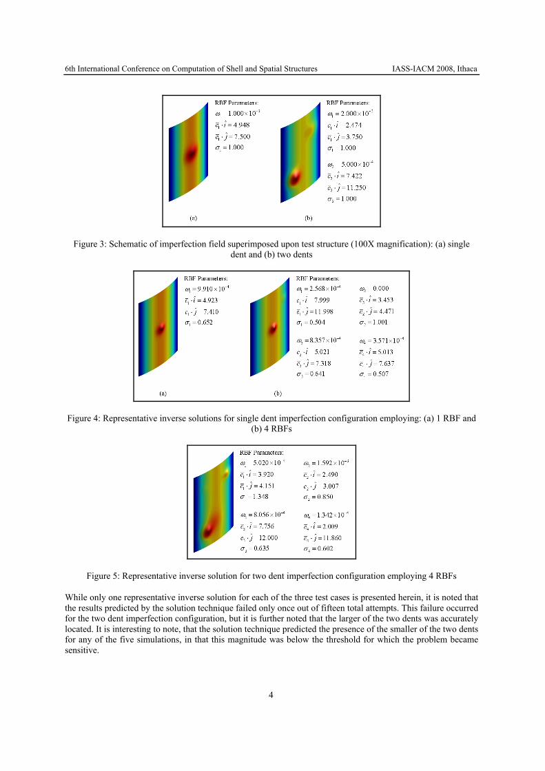
6th International Conference on Computation of Shell and Spatial Structures IASS-IACM 2008, Ithaca
4
Figure 3: Schematic of imperfection field superimposed upon test structure (100X magnification): (a) single dent and (b) two dents
Figure 4: Representative inverse solutions for single dent imperfection configuration employing: (a) 1 RBF and (b) 4 RBFs
Figure 5: Representative inverse solution for two dent imperfection configuration employing 4 RBFs
While only one representative inverse solution for each of the three test cases is presented herein, it is noted that the results predicted by the solution technique failed only once out of fifteen total attempts. This failure occurred for the two dent imperfection configuration, but it is further noted that the larger of the two dents was accurately located. It is interesting to note, that the solution technique predicted the presence of the smaller of the two dents for any of the five simulations, in that this magnitude was below the threshold for which the problem became sensitive.

6th International Conference on Computation of Shell and Spatial Structures IASS-IACM 2008, Ithaca
5
An analysis of the buckling characteristics of each of the inverse solutions provides evidence of close agreement with the target values (i.e. +/- 0.3%). Thus, this solution technique provides a means for the analyst to determine, with a reasonable level of accuracy, the imperfection field of a structure at service load levels. This imperfection field may then be applied to a finite element model of the same structure in order to determine the ultimate capacity of the structure.
5. Conclusions A solution technique, capable of predicting initial imperfections in shell structures, has been presented. The commercial availability of finite element software, coupled with a modified version of the GA tools available in MATLAB, allow for the further development of this solution technique for additional problems.
For the cases considered, this method provides good predictions related to imperfection fields present in the given shell structure; as well as the resulting critical load exhibited by this same imperfect shell.
Acknowledgements The first two authors wish to thank the Office of Naval Research, Program 331, for funding provided for the present research.
References [1] Edlund, B. L. O. Buckling of metallic shells: Buckling and postbuckling behaviour of isotropic shells,
especially cylinders. Structural Control and Health Monitoring, 14:693-713, 2007. [2] Arbocz, J. and Starnes Jr., J.H. Future directions and challenges in shell stability analysis. Thin-Walled
Structures, 40:729-54, 2002. [3] Bielewicz, E. and Gorski, J. Shells with random geometric imperfections simulation based approach.
International Journal of Non-Linear Mechanics, 37:777-84, 2002. [4] ADINA Research and Development, Inc. (2007). ADINA Version 8.4.1. 71 Elton Avenue, Watertown,
Massachusetts 02472. <http://www.adina.com/>. [5] The Mathworks, Inc. (2006). MATLAB Version 7.2.0.232 (R2006a). 3 Apple Hill Drive, Natick,
Massachusetts 01760. <http://www.mathworks.com/>.

Proceedings of the 6th International Conference on
Computation of Shell and Spatial Structures IASS-IACM 2008: “Spanning Nano to Mega”
28-31 May 2008, Cornell University, Ithaca, NY, USA John F. ABEL and J. Robert COOKE (eds.)
Buckling phenomena, analysis and design of axially compressed cylindrical shells with co–existent internal pressure Werner GUGGENBERGER*, Medhanye B. TEKLEAB
Graz University of Technology *Institute for Steel and Shell Structures Lessingstrasse 25, 8010 Graz, Austria [email protected]
Abstract In this paper the elastic and plastic buckling of axially compressed cylindrical metal shell segments is investigated under the side condition of co–exisitent internal pressure. Such non–standard bi–axial loading conditions, leading to meridional membrane compression and simultaneous circumferential membrane tension, are frequently encountered in many structural engineering applications like pipe sections, tanks or silos. The internal pressure loading may be caused by hydrostatic or hydrodynamic earthquake–induced liquid pressure or granular solid pressure in the latter case. The most well–known buckling failure phenomenon connected with this type of loading is the so–called “elephant – foot – type” buckling phenomenon in tanks which is a consequence of the fact that the pre–dominant mode of plastic buckling failure at high pressure levels is represented by more or less axisymmetric shapes of the buckles extending over wide parts of the circumference close to the supported lower boundaries. The main focus of our investigation lies on the analysis of the axisymme-tric plastic buckling phenomenon close to the supported lower shell boundary (elephant foot type buckling) and in the shell interior. In the first case local edge bending disturbances play a leading role, in the second case the presence of axisymmetric geometrical imperfections is of central importance. Comprehensive parametric studies are carried out by variation of the shell slenderness ratio, the shell boundary conditions (fixed versus pinned), a multitude of relevant geometrical imperfection forms and their locations, and finally, the internal pressure ratio in particular. Materially nonlinear only analyses and linear buckling eigenvalue analyses are carried out for reference purposes. The upper limit of (plastic buckling) load bearing capacity is represented by fulfillment of the Mises yield condition by the critical combination of axial compression and meridional tension membrane forces at any location in the free interior of the shell. Edge bending effects do effect plastic buckling, in a negative sense, but they do not effect the purely plastic capacity, i.e. if any geometrically nonlinear effects are neglected.
A clear new understanding of the plastic buckling mode near the boundary is obtained by comparison with the related (axisymmetric) plastic buckling mode in the shell interior. Both modes can be compared for the geometrically perfect as well as for the geometrically imperfect case. Both modes are dominated and limited by the bi–axial Mises membrane yield condition. Considering these common features as basis of comparison it turns out that the plastic boundary buckling mode is not significantly more unfavourable than the related “free shell interior” plastic buckling mode. This is in contrast to some of the existing interpretations and explanations. On the background of results and insights obtained, a coherent new set of buckling design rules was derived which is now based on the bi–axial Mises yield condition.