STRUCTURAL POLICIES AND ECONOMIC RESILIENCE TO SHOCKS

by

Romain Duval, Jørgen Elmeskov and Lukas Vogel1

1. A trend towards more moderate business cycle fluctuations is often quoted as a stylised feature of economic developments in OECD countries over the past several decades. Among the causes frequently cited are better macroeconomic policies that have helped to anchor inflation expectations, a lower incidence and size of outside exogenous shocks, better financial market instruments for risk allocation and a reduced role for and better control of inventories.2 Reflecting the more moderate cycle within countries, cyclical divergences across countries have also tended to shrink over time. As a result, macroeconomic policy requirements have become less divergent across countries. This is obviously important when it comes to countries inside the euro area, where monetary policy settings are by definition identical.

2. Much more controversial is whether, and to what extent, business cycles have become more synchronised across countries. A factor making for synchronous business cycles are common shocks. Historically, oil price hikes have been prominent in this respect, but the oil intensity of OECD economies has tended to decline over time, implying that oil price fluctuations have become less important as a source of large common shocks. Another factor potentially making for synchronous business cycles is propagation of shocks across countries. Here, the increasing trade and financial linkages between countries are likely to have led to faster and stronger transmission of shocks across borders. A particular issue relates to business cycles across euro area countries, with the common currency potentially leading to greater integration and faster transmission, and thereby better alignment of cycles (Frankel and Rose, 1998), but also to greater specialisation and thereby a larger role for idiosyncratic shocks (Krugman, 1993).

3. Apart from idiosyncratic shocks, business cycle divergence across countries may also reflect different responses to common shocks. At issue here is the extent to which some economies are more resilient than others to various shocks. Since 2001, the experience of the large continental European economies contrasts with that of English-speaking OECD countries and many smaller European economies. Many of the shocks hitting countries appeared to be similar between the two groups or even marginally larger in some of the countries in the second group, such as with mass terrorism, the bursting of the equity bubble and corporate governance scandals. Yet, growth performance was generally better in the second group of countries (even adjusting for typically higher rates of potential growth) and even when

1. The authors are, respectively, senior economist, director and economic researcher at the OECD Economics

Department. They would like to thank Christophe André, Benoît Bellone, Jean-Philippe Cotis, Boris Cournède, Sébastien Jean and Dave Rae for helpful discussions. We also thank participants to the March 2007 OECD Working Party No.1 workshop on resilience for comments and suggestions. Remaining errors and omissions are the responsibility of the authors. The views expressed do not necessarily represent those of the OECD or its member governments.

2. See e.g. Dalsgaard et al. (2002); Stock and Watson (2003).

1

recessions occurred they were usually short-lived, with economies bouncing back smartly. It seems unlikely that the differences in performance between the two country groups can be explained by different macroeconomic policy settings, even if these may in some cases have contributed.3 As a result, the hypothesis has emerged that economic resilience is stronger in some countries than in others. Interestingly, and perhaps not coincidentally, the countries seen as more resilient also appear to be the ones that have made most progress on structural reform over the past two decades.

4. Economic resilience may be loosely defined as the ability to maintain output close to potential in the aftermath of shocks. Hence, it comprises at least two dimensions: the extent to which shocks are dampened and the speed with which economies revert to normal following a shock. Structural policies are likely to affect both the strength and persistence of the effects of outside exogenous shocks. Macroeconomic stabilisation policies will also play an important role for resilience, but their effectiveness will also be conditioned by structural policy settings. For example, structural policy settings may affect the strength of the monetary policy transmission mechanism.

5. Against this background, the current paper first reviews simple evidence on business cycle volatility and convergence among OECD countries and within the euro area.4 It then examines at greater length the impact of a range of structural policies on the resilience of economies to shocks, both across countries and over time. A final section sums up the main findings and concludes.

1. Stylised features of business cycles

1.1 Business cycle indicators

6. Business cycles are unobservables and indicators of business cycles rely on the separation of economic developments into trend and cyclical components. This paper focuses exclusively on developments in the volume of GDP and considers three different procedures for decomposing them into trend and cycle.5 Two rely on purely statistical procedures: the Hodrick-Prescott and the Baxter-King filters.6 The cyclical component of GDP, or the output gap, is derived as the difference in per cent between actual and trend GDP. In addition to output gaps derived using these statistical methods, OECD estimates of output gaps are also used. These are constructed as deviations from a trend calculated using a production function, taking as given actual capital stocks and trends of total factor productivity and employment (which in turn is derived based on estimates of the trend participation rates, the NAIRU and trend working hours).7

3. See Cotis and Coppel (2005).

4. Part of this descriptive analysis is an update of prior OECD analysis in Dalsgaard et al. (2002) and Cotis and Coppel (2005).

5. Dalsgaard et al. (2002) provide evidence on cyclical behaviour of a number of demand components.

6. In line with standard practice on quarterly numbers, a HP-filter with a smoothing parameter of 1 600 is used. The Baxter-King filter is implemented so as to remove high-frequency components of less than six and low-frequency components of more than 32 quarters. In practice, in order to mitigate the usual “end-point” problem, these filters are implemented over the period 1960Q1-2008Q4 (1963Q1-2008Q4, 1966Q1-2008Q4 and 1970Q1-2008Q4 for France, Denmark and Korea, respectively), using OECD forecasts (as published in OECD Economic Outlook 80) to extrapolate GDP data up to the fourth quarter of 2008.

7. See e.g. Cotis et al. (2005).

2

7. The three output gap series were calculated on a quarterly basis for 23 OECD countries.8 In addition, a sub-sample of 11 euro area countries is also considered in what follows.9 The statistical measures of output gaps were calculated for the period 1970-2006, whereas the OECD output gap estimate is available only over the period 1980-2006.10

1.2 Main features of business cycle amplitude and convergence

8. Confirming earlier evidence, the cross-country divergence of output gaps appears to have declined over time (Figure 1.1). Standard deviations of output gaps across OECD countries appear to have been broadly halved since the early 1980s. The output gaps based on the three methods provide roughly the same picture in this respect even though the size of cross-country divergences is larger based on the OECD output gap measure than on the two statistical measures. Considering only euro area countries does not change the general impression.

[Figure 1.1. Cyclical divergence across 23 OECD economies, 1970-2006]

9. Reduced cyclical divergence across countries could in principle reflect both a smaller amplitude of cycles within countries and greater synchronisation of cyclical positions across countries. A simple calculation puts the weight on the former explanation: when standard deviations of output gaps are corrected for the size of the average absolute output gap, no signs of increased synchronisation emerge (Figure 1.2). If anything, the trend since 2000 could seem to have been in the direction of greater divergence across countries when assessed based on statistical measures. For euro area countries, signs of convergence were visible up to around 2000, but not thereafter (Figure 1.3).

[Figure 1.2. Cyclical synchronisation across 23 OECD economies, 1970-2006]

[Figure 1.3. Cyclical synchronisation across euro area economies, 1970-2006]

10. The cyclical position of most euro area countries tends to be more correlated with the aggregate euro area cycle than with the US cycle (Figure 1.4). This tendency holds for all the indicators of the output gap considered in this paper, and appears to have strengthened since 1990 as compared with the previous two decades -- corroborating the above impression of some convergence among euro area countries until very recently. Among non-euro area countries, Switzerland also seems to be more aligned with the euro area cycle than with its US counterpart. By contrast, most English-speaking countries (including the UK) tend to have cycles that are more closely aligned with the US cycle than with the euro area (Ireland being the exception), and this tendency has also strengthened since 1990.

[Figure 1.4. Cyclical correlation with the euro area average and the US]

11. An alternative way of exploring tendencies towards greater convergence is to examine whether there is an increased coincidence in time of cyclical troughs and peaks in growth cycles across countries. Any tendency in that direction would see the bars in Figures 1.5 and 1.6 become bigger over time, with a reduced tendency for peak and trough bars to coincide. Again, the impression is that the tendency towards

8. The OECD countries excluded because of insufficient data are the Czech Republic, Hungary, Mexico,

Luxembourg, Poland, the Slovak Republic and Turkey.

9. Output gap series are also calculated for the aggregate euro area economy using the same procedures.

10. The data are taken from the December 2006 OECD Economic Outlook database (OECD, 2006). Among the larger recent data revisions not included in this databank is the upward revision of Greek GDP by about 25% that was announced in late 2006.

3

greater convergence of business cycles has been modest whether for OECD countries at large or just for euro area members.

[Figure 1.5. Business cycle turning points across 23 OECD economies]

[Figure 1.6. Business cycle turning points across 11 euro area countries]

12. Regression analysis can provide a crude separation of cyclical movements into common components across countries and idiosyncratic country variations around the common component. Based on such a decomposition, the respective roles of the common and the idiosyncratic part of the cycle can then be compared over time. More specifically, an OLS estimation of the following panel data equation is run:

GAPit = λt + γ + (γi – γ) + εit [1.1]

where i and t are country and time suffixes, GAPit is the output gap, λt is a time fixed effect which aims to capture an undefined set of shocks that are common to all countries, and γi is a country fixed effect which controls for the fact that output gaps may not necessarily sum to zero over particular sample periods. In this formulation, the common component is λt + γ and the idiosyncratic component (γi – γ) + εit.

13. Figure 1.7 shows the common components estimated for the three different gap measures and for both the 23 OECD countries and 11 of the euro area countries. Overall, the shape is quite similar between the three measures of output gaps, but the common component has a somewhat larger amplitude for the OECD output gap estimates. As well, the common component has a similar shape as between the OECD country sample and the euro area countries, which is perhaps not surprising given that the latter make up close to half of the OECD sample. A trend can be discerned towards peaks and troughs becoming smaller over time.

[Figure 1.7. Common components in business cycles across countries]

14. The idiosyncratic components by construction show no common variation pattern across countries, but they clearly have become smaller over time. This is illustrated in the case of G7 countries in Figure 1.8. The idiosyncratic component also seems to be larger than the common component for most countries (Table 1.1). This is particularly so for small economies with specific specialisation patterns. However, the difference is small, or goes in the opposite direction, for large and/or highly integrated European economies.

[Figure 1.8. Idiosyncratic business cycle components of G-7 economies, 1970-2006]

[Table 1.1. Size of idiosyncratic relative to common fluctuations]

15. As concerns trends over time, a tendency for cycles to become more synchronised should be reflected in a declining importance of the idiosyncratic components relative to the common components. In the sample of 23 OECD countries there is very little sign of this happening on average, although a small majority of countries experience a decline in the variability of the idiosyncratic component relative to that of the common component (Table 1.2)11. Among euro area countries, however, the evidence is more compelling (Table 1.3). The average relative decline in the idiosyncratic component in the euro area appears to be driven by a few countries that had a fairly idiosyncratic cycle in the first part of the period and which subsequently became more aligned with the common cycle (Greece, Netherlands, Portugal). As 11. This conclusion is unchanged if instead the average absolute idiosyncratic component is compared with the

average absolute common component.

4

a result of these developments, idiosyncratic fluctuations appear to have become substantially smaller than the common fluctuations among virtually all euro area countries since 1990.

[Table 1.2. Idiosyncratic relative to common fluctuations over time]

[Table 1.3. Idiosyncratic relative to common fluctuations in the euro area]

1.3 Summing up the descriptive evidence

16. Overall, there is clear evidence that cyclical fluctuations have become smaller over the past three or four decades. By contrast, based on the very simple indicators used here there is no strong evidence to suggest that cycles have become more synchronised across OECD countries. However, among euro area countries, some signs of greater synchronisation are in evidence. The most recent empirical literature does not yield clear-cut results either. Focusing on cross-country correlations between cyclical components and other simple indicators such as those used above, Helbling and Bayoumi (2003) conclude that business cycle linkages have remained unchanged over the 1973-2001 period. Benalal et al. (2006) find evidence of increased business cycle co-movements across euro area economies, but Camacho et al. (2006) obtain no such result using industrial production series and more sophisticated measures of synchronisation -- such as VAR-based or spectral-based approaches. Bergman (2006) even finds that business cycles were more coordinated across euro area members before the implementation of the “hard” exchange rate mechanism (in 1987) than after.

17. The continued importance of idiosyncratic as compared with common cyclical fluctuations, in particular at the level of the OECD at large, may have several causes. One is that economies differ in their degree of resilience to otherwise similar shocks. The rest of the paper explores to what extent different structural policy settings lead to different degrees of resilience across countries.

2. Structural policy determinants of resilience to shocks

18. As already noted, two key dimensions of resilience are the ability of the policy and institutional framework to cushion the initial impact of shocks and to reduce the persistence of the ensuing output gap. In this respect, those policies and institutions that dampen the initial impact of a shock may actually increase its persistence, and vice versa, i.e. they may have conflicting effects on resilience. For instance, strict employment protection legislation (EPL) may deter firms from laying off workers in the short run, thereby supporting employment and private consumption. At the same time, it may slow down the wage adjustment process (Blanchard and Summers, 1986) as well as workers’ reallocation towards more productive jobs, thereby delaying the return of employment and output to their initial levels. Box 1 offers a more coherent theoretical framework for thinking about links between rigidities in labour and product markets and resilience. The upshot is that there is no simple link between policy-induced rigidities and resilience and that the net effect of structural policies in product and labour markets is essentially an empirical issue.

19. Another potential determinant of economic resilience to shocks is the strength of monetary policy transmission channels. Here the expected effect is less ambiguous: in general, the more powerful the monetary transmission mechanism, the smaller and the less persistent the monetary policy and output responses to demand shocks.12 Among the host of factors that contribute to shape monetary transmission channels, the degree of liberalisation of financial markets plays an important role, not least by facilitating 12. In principle, output could also be stabilised in response to demand shocks under a weak transmission

mechanism but this would be associated with an instrument variability that might be unpalatable. In the face of supply shocks, the strength of the transmission mechanism might at worst be irrelevant to the inflation and output pattern.

5

intertemporal consumption smoothing. For example, the degree of mortgage market “completeness” (the range and variety of mortgage products available to borrowers) has been shown to amplify the transmission channel from housing wealth to consumption (Catte et al., 2004). More broadly, econometric analyses of consumption behaviour typically find larger “wealth effects” from housing and financial assets in those countries that have the most liberalised financial markets (see e.g. Deroose, 2006). That said, the use a country can make of an effective monetary transmission mechanism obviously depends on the chosen exchange rate policy.13 For example, small members of a monetary union will not be helped by a strong transmission mechanism when faced with an idiosyncratic shock because monetary policy, calibrated on the union average, will not respond. Likewise, when confronted with a common shock, members of a monetary union can have too much of a good thing in the sense that a transmission mechanism that is stronger than average, together with a monetary policy response that is calibrated on the average, could be destabilizing. The analysis below controls for the influence of exchange rate policy as a constraint on monetary policy that may make it more difficult to stabilise the economy in the face of idiosyncratic shocks and/or heterogeneous propagation mechanisms of common shocks.

20. Fiscal policy may also affect resilience patterns via two main channels. First, automatic stabilisers are expected to dampen the impact of shocks. Strong automatic stabilisers are typically associated with large public sectors, which in turn partly reflect some of the structural policies mentioned above -- such as high and long-lasting unemployment benefits. Second, discretionary fiscal policy may be stabilising or destabilising, depending on whether it is counter or pro-cyclical. Here, one might expect government size, which allows strong automatic stabilisers, to be associated with a reduced need for discretionary fiscal impulses. This may not always be the case in practice, however. Evidence in Ahrend et al. (2006) suggests that several countries with large public sectors have supplemented automatic stabilisers with sizeable discretionary (counter-cyclical) actions over the past two decades. These were on balance stabilising in Nordic countries, but destabilising in many euro-area countries. Fiscal policy was more in line with expectations in countries with smaller public sectors -- such as a number of English-speaking and Asian OECD countries --, with sizeable discretionary impulses contributing to output stabilisation.

Box 1. Theoretical considerations on the link between product and labour market rigidities and resilience Modern business cycle theory offers a systematic take on the link between rigidities and resilience. In a basic

New Keynesian model, greater (nominal) wage and/or price stickiness flattens the (New Keynesian) Phillips curve and increases the sacrifice ratio. In turn, under optimal monetary policy,1 an independent central bank credibly committed to medium-term price stability will react less aggressively to most shocks -- including temporary but persistent cost-push or technology shocks -- thereby engineering a smaller but more prolonged output gap response (see e.g. Altissimo et al., 2006). The intuition is that since nominal rigidities worsen the inflation-output variability trade-off, a more aggressive policy reaction to a cost-push shock would induce large output losses for a limited gain in terms of reduced inflation.2 By contrast, in the case of pure demand shocks, rigidities may be of little influence since monetary policy can readily stabilise aggregate demand without facing any trade-off between output and inflation stabilisation.

Any policy or institution that increases wage and/or price stickiness would therefore be expected to lead to a smaller but more persistent output reaction to certain shocks. Among the many theoretical underpinnings of price stickiness, imperfect competition in product markets features prominently, e.g. through menu costs or coordination failure3 approaches.4 On the empirical side, there is now fairly strong evidence at the microeconomic level that firms tend to reset their prices more frequently in more competitive markets, lending some support to the view that low product market competition increases price stickiness (see e.g. the recent analysis carried out within the context of the Eurosystem Inflation Persistence Network, including inter alia Alvaréz et al., 2006, and Fabiani et al., 2006). Likewise, among the various theoretical explanations for wage stickiness, some authors have stressed the role played by labour market policies and institutions.5 For example, stringent EPL and/or high coverage of collective agreements bargained between unions and firms may slow down the adjustment of labour contracts in the face of shocks and thereby be conducive to nominal wage rigidities (Holden, 1994, 2004).

Like price stickiness, real wage rigidities flatten the Phillips curve and increase the sacrifice ratio. Real wage rigidities may be strengthened, for example, by high unemployment benefit replacement rates available over long 13. The exchange rate is part of the monetary transmission mechanism, but this aspect is not explicitly covered

in the current analysis.

6

periods. Ceteris paribus, rigid real wages should induce a less aggressive monetary policy response, and therefore a smaller but more persistent output reaction, to a variety of shocks. However, unlike price stickiness, real wage rigidities also increase the persistence of inflation, which should prompt monetary authorities to be more aggressive, thereby engineering a larger but less persistent output reaction to shocks. The latter effect may dominate in practice.6 To sum up, while nominal rigidities should lead to smaller but more persistent output gaps, real rigidities might go in the opposite direction.7 In both cases, the implications for resilience are expected to be ambiguous a priori.8________ 1. Minimising a quadratic loss function defined over both inflation and output gaps.

2. Given the convexity of the central bank’s welfare loss function, such a policy response would not be optimal. Another reason for the central bank to react less aggressively to a cost-push shock in the presence of price stickiness is that the initial impact of the shock on inflation will be smaller, for example because firms reset prices less frequently.

3. Co-ordination failure relates to the observation that in oligopolistic markets, following a shock, firms may choose not to change their prices unless their competitors move first.

4. Furthermore, Rotemberg and Woodford (1991) have suggested that during upswings, oligopolistic firms have greater incentives to free ride on other firms’ efforts to maintain collusive price behaviour, so that mark-ups should fall. This counter-cyclicality of mark-ups provides another reason to expect that low product market competition flattens the Phillips curve.

5. Other factors may also play a role. For example, in conditions of low and stable inflation, contracts may lengthen which could induce greater nominal inertia.

6. Work undertaken as part of this paper shows that when real wage rigidities à la Blanchard and Galí (2005) are introduced in an otherwise basic New Keynesian model, the optimal monetary response to a cost-push shock is more aggressive than under flexible real wages. This more aggressive policy response is associated with a larger but less persistent impact on the output gap. A similar conclusion appears to hold for technology shocks.

7. Model simulations suggest that this conclusion also holds within a monetary union. In a member country with an above-average degree of nominal rigidity, the initial impact of a common cost-push shock on prices is smaller. This results in a competitiveness gain which in turn mitigates the impact of the common shock on the output gap. However, this comes at the cost of a more persistent output gap, as more flexible countries quickly restore their competitiveness through the larger negative impact on inflation of their negative output gap. By contrast, in a member country with an above-average degree of real wage rigidity, the dominant effect is that the common cost-push shock brings about higher wages and therefore a loss of competitiveness. This in turn results in a larger initial impact of the common shock on the output gap.8. It should also be stressed that the empirical notion of output gap used in this paper differs from the theoretical concept of output gap featured in New Keynesian models. The former is essentially the difference between actual and smoothed GDP, while the latter is the difference between actual and “natural” output, where -- in line with the real business cycle literature -- natural output may be quite volatile, e.g. due to temporary technology shocks.

2.1 Modelling strategy and preliminary cross-country comparison of business cycle patterns

21. With resilience determined by both amplification and persistence mechanisms, an empirical investigation of the phenomenon has to be dynamic in nature. This sub-section explores the determinants of cross-country business cycle patterns by means of dynamic, panel data output gap equations. As the first section has shown, most features of business cycles appear to hold independently of the exact measure chosen. Therefore, the analysis undertaken below focuses on only one of these, namely the OECD output gap measure. Another obvious consideration is that the modelled dynamics should fit OECD output gap patterns. As discussed in Box 2, visual inspection and specification tests point to an AR(2) specification for describing output gaps (as well as unemployment gaps, dealt with below in Box 3).

22. As a starting point, the following dynamic (non-linear) panel regression is estimated for a sample of 20 OECD countries14 using annual OECD output gap data over the period 1982-2003:15

14. Australia, Austria, Belgium, Canada, Denmark, Finland, France, Germany, Ireland, Italy, Japan,

Netherlands, New Zealand, Norway, Portugal, Spain, Sweden, Switzerland, United Kingdom, United States.

15. The choice of the time period is driven by the availability of policy and institutional indicators, in particular the OECD EPL index which starts in 1982.

7

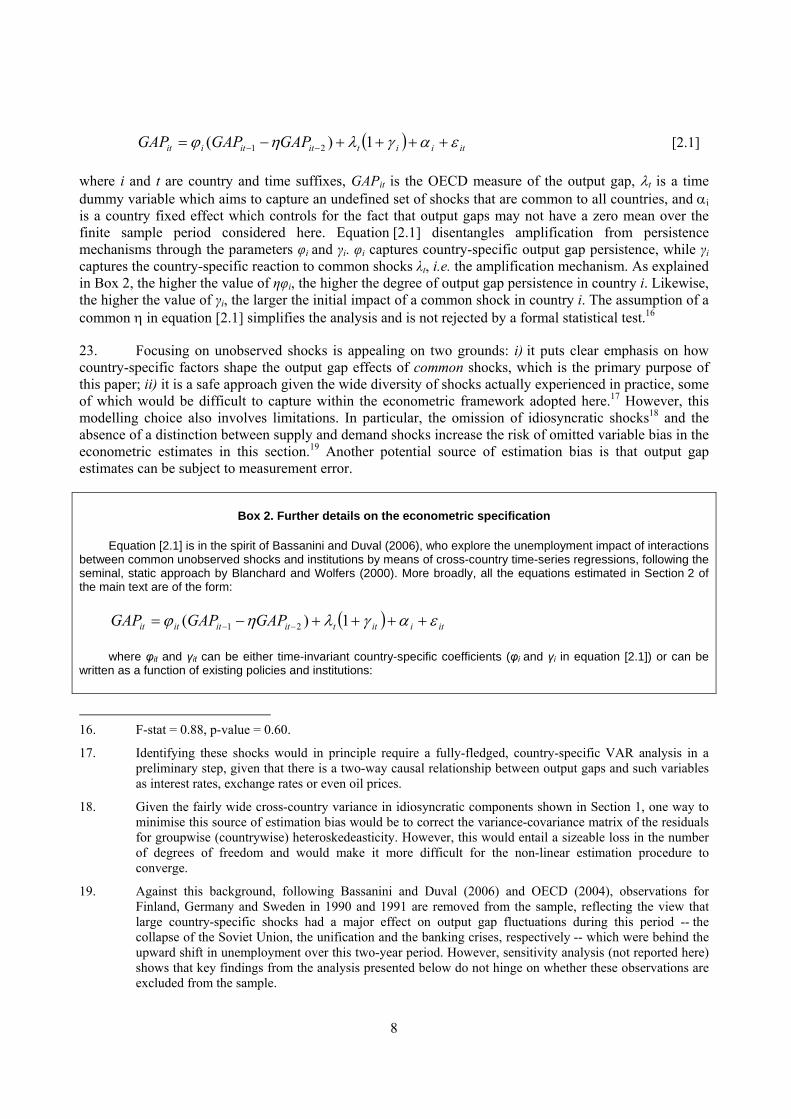
( ) itiitititiit GAPGAPGAP εαγληϕ ++++−= −− 1)( 21 [2.1]

where i and t are country and time suffixes, GAPit is the OECD measure of the output gap, λt is a time dummy variable which aims to capture an undefined set of shocks that are common to all countries, and αi is a country fixed effect which controls for the fact that output gaps may not have a zero mean over the finite sample period considered here. Equation [2.1] disentangles amplification from persistence mechanisms through the parameters φi and γi. φi captures country-specific output gap persistence, while γi captures the country-specific reaction to common shocks λt, i.e. the amplification mechanism. As explained in Box 2, the higher the value of ηφi, the higher the degree of output gap persistence in country i. Likewise, the higher the value of γi, the larger the initial impact of a common shock in country i. The assumption of a common η in equation [2.1] simplifies the analysis and is not rejected by a formal statistical test.16

23. Focusing on unobserved shocks is appealing on two grounds: i) it puts clear emphasis on how country-specific factors shape the output gap effects of common shocks, which is the primary purpose of this paper; ii) it is a safe approach given the wide diversity of shocks actually experienced in practice, some of which would be difficult to capture within the econometric framework adopted here.17 However, this modelling choice also involves limitations. In particular, the omission of idiosyncratic shocks18 and the absence of a distinction between supply and demand shocks increase the risk of omitted variable bias in the econometric estimates in this section.19 Another potential source of estimation bias is that output gap estimates can be subject to measurement error.

Box 2. Further details on the econometric specification

Equation [2.1] is in the spirit of Bassanini and Duval (2006), who explore the unemployment impact of interactions between common unobserved shocks and institutions by means of cross-country time-series regressions, following the seminal, static approach by Blanchard and Wolfers (2000). More broadly, all the equations estimated in Section 2 of the main text are of the form:

( ) itiittitititit GAPGAPGAP εαγληϕ ++++−= −− 1)( 21

where φit and γit can be either time-invariant country-specific coefficients (φi and γi in equation [2.1]) or can be written as a function of existing policies and institutions:

16. F-stat = 0.88, p-value = 0.60.

17. Identifying these shocks would in principle require a fully-fledged, country-specific VAR analysis in a preliminary step, given that there is a two-way causal relationship between output gaps and such variables as interest rates, exchange rates or even oil prices.

18. Given the fairly wide cross-country variance in idiosyncratic components shown in Section 1, one way to minimise this source of estimation bias would be to correct the variance-covariance matrix of the residuals for groupwise (countrywise) heteroskedeasticity. However, this would entail a sizeable loss in the number of degrees of freedom and would make it more difficult for the non-linear estimation procedure to converge.

19. Against this background, following Bassanini and Duval (2006) and OECD (2004), observations for Finland, Germany and Sweden in 1990 and 1991 are removed from the sample, reflecting the view that large country-specific shocks had a major effect on output gap fluctuations during this period -- the collapse of the Soviet Union, the unification and the banking crises, respectively -- which were behind the upward shift in unemployment over this two-year period. However, sensitivity analysis (not reported here) shows that key findings from the analysis presented below do not hinge on whether these observations are excluded from the sample.

8

( ∑ −+=j

jjit

jit XX )( ..ϕϕϕ and ∑ −=

k

kkit

kit XX )( ..γγ in equation [2.2]).

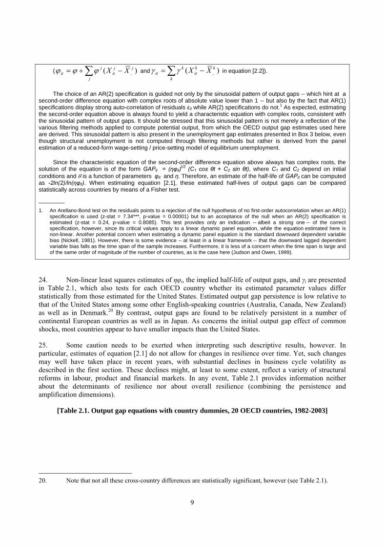
The choice of an AR(2) specification is guided not only by the sinusoidal pattern of output gaps -- which hint at a second-order difference equation with complex roots of absolute value lower than 1 -- but also by the fact that AR(1) specifications display strong auto-correlation of residuals εit while AR(2) specifications do not.1 As expected, estimating the second-order equation above is always found to yield a characteristic equation with complex roots, consistent with the sinusoidal pattern of output gaps. It should be stressed that this sinusoidal pattern is not merely a reflection of the various filtering methods applied to compute potential output, from which the OECD output gap estimates used here are derived. This sinusoidal pattern is also present in the unemployment gap estimates presented in Box 3 below, even though structural unemployment is not computed through filtering methods but rather is derived from the panel estimation of a reduced-form wage-setting / price-setting model of equilibrium unemployment.

Since the characteristic equation of the second-order difference equation above always has complex roots, the solution of the equation is of the form GAPit = (ηφit)t/2 (C1 cos θt + C2 sin θt), where C1 and C2 depend on initial conditions and θ is a function of parameters φit and η. Therefore, an estimate of the half-life of GAPit can be computed as -2ln(2)/ln(ηφit). When estimating equation [2.1], these estimated half-lives of output gaps can be compared statistically across countries by means of a Fisher test.

________

1. An Arellano-Bond test on the residuals points to a rejection of the null hypothesis of no first-order autocorrelation when an AR(1) specification is used (z-stat = 7.34***, p-value = 0.00001) but to an acceptance of the null when an AR(2) specification is estimated (z-stat = 0.24, p-value = 0.8085). This test provides only an indication -- albeit a strong one -- of the correct specification, however, since its critical values apply to a linear dynamic panel equation, while the equation estimated here is non-linear. Another potential concern when estimating a dynamic panel equation is the standard downward dependent variable bias (Nickell, 1981). However, there is some evidence -- at least in a linear framework -- that the downward lagged dependent variable bias falls as the time span of the sample increases. Furthermore, it is less of a concern when the time span is large and of the same order of magnitude of the number of countries, as is the case here (Judson and Owen, 1999).

24. Non-linear least squares estimates of ηφi, the implied half-life of output gaps, and γi are presented in Table 2.1, which also tests for each OECD country whether its estimated parameter values differ statistically from those estimated for the United States. Estimated output gap persistence is low relative to that of the United States among some other English-speaking countries (Australia, Canada, New Zealand) as well as in Denmark.20 By contrast, output gaps are found to be relatively persistent in a number of continental European countries as well as in Japan. As concerns the initial output gap effect of common shocks, most countries appear to have smaller impacts than the United States.

25. Some caution needs to be exerted when interpreting such descriptive results, however. In particular, estimates of equation [2.1] do not allow for changes in resilience over time. Yet, such changes may well have taken place in recent years, with substantial declines in business cycle volatility as described in the first section. These declines might, at least to some extent, reflect a variety of structural reforms in labour, product and financial markets. In any event, Table 2.1 provides information neither about the determinants of resilience nor about overall resilience (combining the persistence and amplification dimensions).

[Table 2.1. Output gap equations with country dummies, 20 OECD countries, 1982-2003]

20. Note that not all these cross-country differences are statistically significant, however (see Table 2.1).

9

2.2 The impact of labour and product market regulation on business cycle patterns

Correlations between policies and resilience parameters

26. As preliminary evidence of the effects of labour and product market regulation on business cycle patterns, the country-specific persistence and amplification coefficients φi and γi estimated in Table 2.1 are retrieved and regressed on the following indicators (averaged for each country over the period 1982-2003) in separate regressions: 21

• The unemployment benefit replacement rate (averaged across a variety of income levels, family situations and unemployment durations).

• The stringency of employment protection legislation for regular workers (EPL).

• The stringency of product market regulation (PMR) across seven non-manufacturing industries.22

• Collective bargaining coverage, i.e. the share of workers covered by a collective agreement, a measure of union influence in wage bargaining.23

• The degree of centralisation/co-ordination of wage bargaining, a proxy for the concept of “corporatism” which has received widespread attention in the comparative political economy literature. In practice, the variable entered in the econometric estimates is a “low corporatism” dummy variable, which equals 1 if bargaining is decentralised and uncoordinated and zero otherwise.

27. Cross-country correlation coefficients between persistence and amplification coefficients φi and γi on the one hand, and the above policy indicators on the other, are presented in Table 2.2. Given that persistence and amplification coefficients are estimated rather than observed -- so that standard statistical inference could be misleading -- the critical values used to assess the statistical significance of each correlation coefficient are obtained by bootstrapping the regression residuals. Strict EPL, stringent PMR and a high degree of corporatism appear to be negatively correlated with the initial impact of shocks but positively with output gap persistence. Similar but insignificant correlation signs are obtained for collective bargaining coverage and the unemployment benefit replacement rate. In a nutshell, the results from Table 2.2 suggest that strict labour and product market regulations may dampen the initial impact of a common shock while making it more persistent.

21. See data appendix for full details on data sources and methods. These indicators are time-varying and

available at an annual frequency, with the exception of collective bargaining coverage which is time-invariant (country average over 1980-2000) due to lack of data at an annual frequency over the sample period.

22. This sector-based PMR indicator is used in this paper because it covers the whole sample period, unlike the OECD’s economy-wide indicator which is available only for 1998 and 2003. One drawback is that changes in the indicator for non-manufacturing sectors do not incorporate all aspects of regulatory reforms that have been undertaken by a number of OECD countries in the past decades, such as administrative reforms affecting all sectors. As a result, the resilience effects of regulatory reforms may not be fully captured by the econometric estimates presented in this paper.

23. This variable is less imperfect than union density, not least because administrative extension practices -- which remain in place in a number of continental European countries -- extend collective agreements to the non-affiliated, providing unions with greater bargaining power in practice than union membership rates would suggest.

10

[Table 2.2. Cross-country correlation coefficients between persistence/amplification coefficients and labour/product market policy indicators]

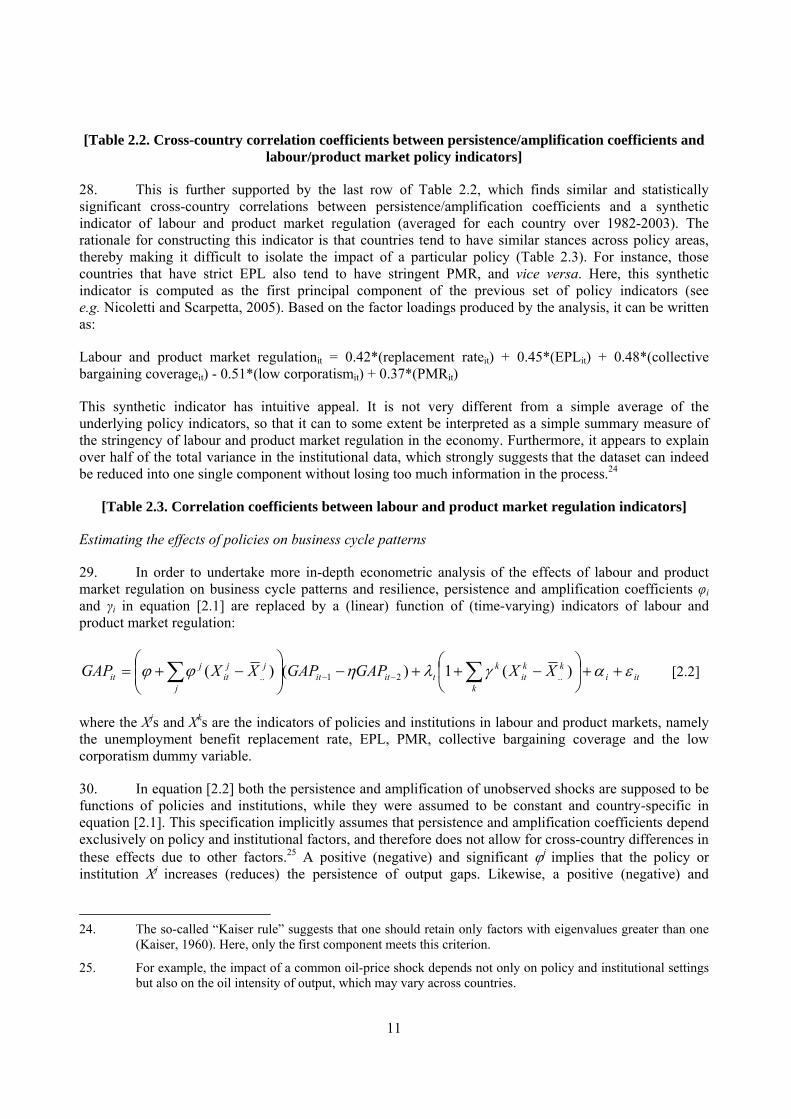
28. This is further supported by the last row of Table 2.2, which finds similar and statistically significant cross-country correlations between persistence/amplification coefficients and a synthetic indicator of labour and product market regulation (averaged for each country over 1982-2003). The rationale for constructing this indicator is that countries tend to have similar stances across policy areas, thereby making it difficult to isolate the impact of a particular policy (Table 2.3). For instance, those countries that have strict EPL also tend to have stringent PMR, and vice versa. Here, this synthetic indicator is computed as the first principal component of the previous set of policy indicators (see e.g. Nicoletti and Scarpetta, 2005). Based on the factor loadings produced by the analysis, it can be written as:

Labour and product market regulationit = 0.42*(replacement rateit) + 0.45*(EPLit) + 0.48*(collective bargaining coverageit) - 0.51*(low corporatismit) + 0.37*(PMRit)

This synthetic indicator has intuitive appeal. It is not very different from a simple average of the underlying policy indicators, so that it can to some extent be interpreted as a simple summary measure of the stringency of labour and product market regulation in the economy. Furthermore, it appears to explain over half of the total variance in the institutional data, which strongly suggests that the dataset can indeed be reduced into one single component without losing too much information in the process.24

[Table 2.3. Correlation coefficients between labour and product market regulation indicators]

Estimating the effects of policies on business cycle patterns

29. In order to undertake more in-depth econometric analysis of the effects of labour and product market regulation on business cycle patterns and resilience, persistence and amplification coefficients φi and γi in equation [2.1] are replaced by a (linear) function of (time-varying) indicators of labour and product market regulation:

itik

kkit

ktitit

j

jjit

jit XXGAPGAPXXGAP εαγληϕϕ ++⎟

⎠

⎞⎜⎝

⎛−++−⎟⎟

⎠

⎞⎜⎜⎝

⎛−+= ∑∑ −− )(1)()( ..21.. [2.2]

where the Xjs and Xks are the indicators of policies and institutions in labour and product markets, namely the unemployment benefit replacement rate, EPL, PMR, collective bargaining coverage and the low corporatism dummy variable.

30. In equation [2.2] both the persistence and amplification of unobserved shocks are supposed to be functions of policies and institutions, while they were assumed to be constant and country-specific in equation [2.1]. This specification implicitly assumes that persistence and amplification coefficients depend exclusively on policy and institutional factors, and therefore does not allow for cross-country differences in these effects due to other factors.25 A positive (negative) and significant ϕj implies that the policy or institution Xj increases (reduces) the persistence of output gaps. Likewise, a positive (negative) and

24. The so-called “Kaiser rule” suggests that one should retain only factors with eigenvalues greater than one

(Kaiser, 1960). Here, only the first component meets this criterion.

25. For example, the impact of a common oil-price shock depends not only on policy and institutional settings but also on the oil intensity of output, which may vary across countries.

11

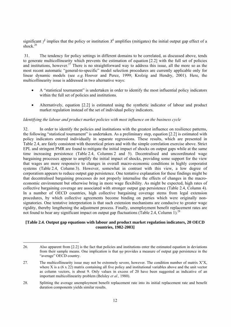
significant γk implies that the policy or institution Xk amplifies (mitigates) the initial output gap effect of a shock.26

31. The tendency for policy settings in different domains to be correlated, as discussed above, tends to generate multicollinearity which prevents the estimation of equation [2.2] with the full set of policies and institutions, however.27 There is no straightforward way to address this issue, all the more so as the most recent automatic “general-to-specific” model selection procedures are currently applicable only for linear dynamic models (see e.g. Hoover and Perez, 1999; Krolzig and Hendry, 2001). Here, the multicollinearity issue is addressed in two alternative ways:

• A “statistical tournament” is undertaken in order to identify the most influential policy indicators within the full set of policies and institutions.

• Alternatively, equation [2.2] is estimated using the synthetic indicator of labour and product market regulation instead of the set of individual policy indicators.

Identifying the labour and product market policies with most influence on the business cycle

32. In order to identify the policies and institutions with the greatest influence on resilience patterns, the following “statistical tournament” is undertaken. As a preliminary step, equation [2.2] is estimated with policy indicators entered individually in separate regressions. These results, which are presented in Table 2.4, are fairly consistent with theoretical priors and with the simple correlation exercise above. Strict EPL and stringent PMR are found to mitigate the initial impact of shocks on output gaps while at the same time increasing persistence (Table 2.4, Columns 2 and 5). Decentralised and uncoordinated wage bargaining processes appear to amplify the initial impact of shocks, providing some support for the view that wages are more responsive to changes in overall macro-economic conditions in highly corporatist systems (Table 2.4, Column 3). However, somewhat in contrast with this view, a low degree of corporatism appears to reduce output gap persistence. One tentative explanation for these findings might be that decentralised bargaining processes do not properly internalise the effects of changes in the macro-economic environment but otherwise bring in more wage flexibility. As might be expected, high rates of collective bargaining coverage are associated with stronger output gap persistence (Table 2.4, Column 4). In a number of OECD countries, high collective bargaining coverage stems from legal extension procedures, by which collective agreements become binding on parties which were originally non-signatories. One tentative interpretation is that such extension mechanisms are conducive to greater wage rigidity, thereby lengthening the adjustment process. Finally, unemployment benefit replacement rates are not found to bear any significant impact on output gap fluctuations (Table 2.4, Column 1).28

[Table 2.4. Output gap equations with labour and product market regulation indicators, 20 OECD countries, 1982-2003]

26. Also apparent from [2.2] is the fact that policies and institutions enter the estimated equation in deviations

from their sample means. One implication is that ηφ provides a measure of output gap persistence in the “average” OECD country.

27. The multicollinearity issue may not be extremely severe, however. The condition number of matrix X’X, where X is a (6 x 22) matrix containing all five policy and institutional variables above and the unit vector as column vectors, is about 9. Only values in excess of 20 have been suggested as indicative of an important multicollinearity problem (Belsley et al., 1980).

28. Splitting the average unemployment benefit replacement rate into its initial replacement rate and benefit duration components yields similar results.

12

33. As a second step, those persistence and/or amplification terms that are insignificant in the individual regressions are seen as having no robust impact on output gap patterns and are thus dropped from the analysis. This leaves a set of seven significant policy and institutional terms to focus upon, four related to persistence and three concerned with the initial impact of shocks. Equation [2.2] is then estimated with two terms for all possible pairs of policies and institutions among the seven remaining terms. Those terms that are found to be insignificant (at the 10% confidence level) in at least one of the regressions are then discarded, and the remaining ones are built upon to estimate equations with three variables. The selection procedure continues until a final model is selected. It can be safely inferred from this “statistical tournament” that “surviving” policy and/or institutional terms significantly affect output gap patterns. By contrast, no firm conclusions can be drawn from this procedure as regards discarded terms -- given that possible significant impacts may have been obscured by the even more significant effect of other variables -- and, more broadly, as regards the “true” model.

34. The final model selected through this procedure contains two variables, namely EPL and PMR (Table 2.4, Column 6). It is reassuring to note that estimating the full model from the outset would point to a similar selection (Table 2.4, Column 7). There is therefore robust evidence that stringent PMR dampens the initial impact of shocks while strict EPL increases persistence. Overall, these findings are consistent with those obtained by Bassanini and Duval (2006) regarding unemployment patterns, although unemployment benefits are also found to have a robust positive effect on persistence in their paper.

35. For the average OECD country, the estimated half-life of output gaps is 1.8 years. Taken at face value, the estimates suggest that for this “average” OECD country, a two standard deviation decline in EPL stringency would reduce the half-life of output gaps by almost half a year.29 Similarly, a two standard deviation decline in PMR would raise the initial impact of a shock by about one-half. While the magnitude of the estimated effects does not look implausible, caution should be exercised when interpreting them. As already noted, it is plausible that although the “statistical tournament” approach helps single out the most significant policies and institutions, it is unable to select the “true” model. For instance, the separate impact of EPL and collective bargaining coverage may be difficult to disentangle insofar as they are highly correlated and interact with shocks through comparable channels.

The impact of overall labour and product market policies on the business cycle

36. An alternative approach is to re-estimate equation [2.2] using the synthetic indicator of labour and product market regulation as the only structural policy variable. As expected, amplification and persistence coefficients are of opposite signs and they are statistically significant at the 1% confidence level (Table 2.5, Column 1). This strongly suggests that strict labour and product market regulation dampens the initial impact of a common shock but makes it more persistent.

[Table 2.5. Output gap equations with synthetic indicators of labour and product market regulation, 20 OECD countries, 1982-2003]

29. By construction, the values of both the EPL indicator and that of product market regulation for seven non-

manufacturing industries range from 0 to 6. In 2003, their average values across the 20 countries included in the sample were equal to 1.84 and 2.1, and their standard deviations were equal to 0.87 and 0.55, respectively. For the “average” OECD country, a decline in EPL by two standard deviations would be equivalent to bringing it down to the stance observed in the some of the most liberal OECD countries (Canada and the United Kingdom, where EPL is estimated to be slightly more stringent than in the most liberal country, namely the United States). Likewise, a decline in PMR by two standard deviations would be equivalent to undertaking product market liberalisation of the same order of magnitude as that which has taken place in the average OECD country over the past ten years.

13

2.3 Monetary and financial drivers of business cycle patterns

37. As noted earlier, output gap dynamics in the aftermath of a shock depends not only on supply-side rigidities in the economy but also on the monetary policy response as well as on the strength of the monetary policy transmission channel. A tentative and limited attempt to tackle these issues is provided here by considering three monetary and financial variables that may impact on resilience. First, household mortgage debt (as a share of GDP) can be seen as an indicator of financial market flexibility -- it tends to bear a negative relationship with measures of mortgage market regulation30 -- and as such it is expected to strengthen monetary policy transmission. Second, a flexible exchange rate dummy variable31 is aimed at capturing whether domestic monetary policy can react to shocks and thereby (under efficient monetary policy) both cushion the initial impact of shocks and make them less persistent.32 Finally, a financial intermediation variable, computed as the ratio of total bank credit to stock market value traded, captures the extent to which the financial system is dominated by bank intermediation rather than by market institutions. Bank-based systems might conduce to slower initial pass-through but more persistence of shocks than market-based systems (see e.g. Artis, 2005).33 Table 2.6 finds estimated output gap persistence to be correlated negatively across countries with household mortgage debt and the flexible exchange rate dummy variable, and positively with financial intermediation.

[Table 2.6. Cross-country correlation coefficients between persistence/amplification coefficients and monetary/financial variables]

38. Table 2.5 extends the baseline equation featuring the synthetic indicator of labour and product market regulation (Table 2.5, Column 1) to incorporate the indicator of household mortgage debt (Column 2), the flexible exchange rate dummy variable (Column 3), or the financial intermediation variable (Column 4). These extensions yield only one significant finding at the 5% confidence level, namely that high levels of household mortgage debt tend to lower output gap persistence, consistent with the view that they strengthen monetary transmission. Furthermore, only household mortgage debt survives a “statistical tournament” between the three monetary and financial variables.34 Reflecting this, a final, preferred specification features labour and product market regulation and household mortgage debt in the persistence term and labour and product market regulation in the amplification term (Column 5). While 30. See Catte et al. (2004). Household mortgage debt is expressed as a share of GDP and is time-invariant

(country average over 1990-2002), due to lack of data at an annual frequency for most countries over the sample period. See data appendix for details.

31. This dummy variable takes value 1 if the country is not engaged in any fixed exchange rate agreement in year t and zero otherwise. See data appendix for details.

32. For euro area countries, which according to Section 1 have seen an increased synchronisation of cycles, the common monetary policy may of course react to common shocks. The dummy variable is not able to capture such nuances, which could explain its lack of significance in the regressions discussed below. As well, it could be argued that what matters is the combination of monetary policy autonomy and the strength of the transmission mechanism, i.e. that the two variables should be interacted. However, such interactions (not reported here) were tested but appeared to be statistically insignificant.

33. See data appendix. The value of trades on domestic shares is used as denominator because the main alternative, namely stock market capitalisation, does not measure the amount of funding available to firms but rather the discounted value of future earnings. Stock market capitalisation provides an indication of the size rather than the activity of stock markets. That said, it should be acknowledged that stock market value traded primarily captures turnover in stock markets and therefore is also an imperfect proxy for firms’ access to capital.

34. It should be stressed that this variable is particularly robust since it would also survive the statistical tournament between labour and product market regulation indicators carried out in the previous section, and would therefore appear in the “final” model along with the other variables selected.

14

household mortgage debt -- and the strength of monetary transmission channels more broadly – would be expected to improve resilience mainly under flexible exchange rates, in practice no significant interaction was found here between these two variables.

2.4 Sensitivity analysis

Using alternative output gap measures

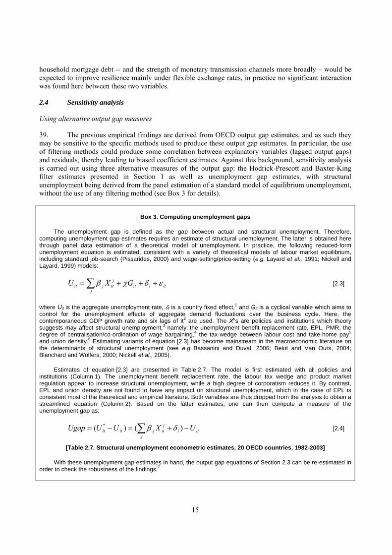
39. The previous empirical findings are derived from OECD output gap estimates, and as such they may be sensitive to the specific methods used to produce these output gap estimates. In particular, the use of filtering methods could produce some correlation between explanatory variables (lagged output gaps) and residuals, thereby leading to biased coefficient estimates. Against this background, sensitivity analysis is carried out using three alternative measures of the output gap: the Hodrick-Prescott and Baxter-King filter estimates presented in Section 1 as well as unemployment gap estimates, with structural unemployment being derived from the panel estimation of a standard model of equilibrium unemployment, without the use of any filtering method (see Box 3 for details).

Box 3. Computing unemployment gaps

The unemployment gap is defined as the gap between actual and structural unemployment. Therefore, computing unemployment gap estimates requires an estimate of structural unemployment. The latter is obtained here through panel data estimation of a theoretical model of unemployment. In practice, the following reduced-form unemployment equation is estimated, consistent with a variety of theoretical models of labour market equilibrium, including standard job-search (Pissarides, 2000) and wage-setting/price-setting (e.g. Layard et al., 1991; Nickell and Layard, 1999) models:

[2.3] itiitj

jitjit GXU εδχβ +++= ∑

where Uit is the aggregate unemployment rate, δi is a country fixed effect,1 and Git is a cyclical variable which aims to control for the unemployment effects of aggregate demand fluctuations over the business cycle. Here, the contemporaneous GDP growth rate and six lags of it2 are used. The Xj’s are policies and institutions which theory suggests may affect structural unemployment,3 namely: the unemployment benefit replacement rate, EPL, PMR, the degree of centralisation/co-ordination of wage bargaining,4 the tax-wedge between labour cost and take-home pay5 and union density.6 Estimating variants of equation [2.3] has become mainstream in the macroeconomic literature on the determinants of structural unemployment (see e.g. Bassanini and Duval, 2006; Belot and Van Ours, 2004; Blanchard and Wolfers, 2000; Nickell et al., 2005).

Estimates of equation [2.3] are presented in Table 2.7. The model is first estimated with all policies and institutions (Column 1). The unemployment benefit replacement rate, the labour tax wedge and product market regulation appear to increase structural unemployment, while a high degree of corporatism reduces it. By contrast, EPL and union density are not found to have any impact on structural unemployment, which in the case of EPL is consistent most of the theoretical and empirical literature. Both variables are thus dropped from the analysis to obtain a streamlined equation (Column 2). Based on the latter estimates, one can then compute a measure of the unemployment gap as:

[2.4] itij

jitjitit UXUUUgap −+=−= ∑ )()( * δβ

[Table 2.7. Structural unemployment econometric estimates, 20 OECD countries, 1982-2003]

With these unemployment gap estimates in hand, the output gap equations of Section 2.3 can be re-estimated in order to check the robustness of the findings.7

15

________

1. The inclusion of country effects -- which are found to be jointly significant -- aims to control for omitted, country-specific determinants of structural unemployment.

2. Starting from a model with 10 lags, insignificant lags were eliminated sequentially until all remaining lags were found to be significant.

3. See e.g. Bassanini and Duval (2006), Nickell and Layard (1999), Nickell (1997, 1998), Pissarides (2000).

4. In line with Bassanini and Duval (2006), its influence is captured in Table 2.7 through a dummy for “high corporatism” -- instead of the “low corporatism” dummy used above.

5. See data appendix for details on sources and methods.

6. Union density, which is defined as the rate of union membership (see data appendix for details), aims to capture union power. While the rate of collective bargaining coverage would be arguably a better proxy -- which is why it was used in the econometric analysis above, it is not available over the whole sample for most OECD countries and therefore cannot be used here.

7. Ideally, one would rather estimate a dynamic unemployment equation in one step, identifying simultaneously the policy determinants of equilibrium unemployment and those of short-run unemployment dynamics. However, compared with the two-step estimation approach followed here, the large number of additional parameters to be estimated would imply a sizeable loss in the number of degrees of freedom and would make it more difficult for the non-linear estimation procedure to converge.

40. Table 2.8 presents the re-estimation of three key equations -- the model selected from the “statistical tournament” on labour and product market policies (Table 2.4, Column 6), the model using the synthetic indicator of labour and product market regulation (Table 2.5, Column 1) and the model incorporating the synthetic indicator of labour and product market regulation and household mortgage debt (Table 2.5, Column 5) -- using the three alternative gap estimates. The main conclusion is that the findings are reasonably robust to the method used to construct the gaps. The only two noticeable differences with respect to previous results are the following: i) Labour and product market regulation is no longer found to mitigate the initial impact of shocks when unemployment gap estimates are used; household mortgage debt no longer appears to raise gap persistence when Baxter-King filter estimates are used.

[Table 2.8. Equations with alternative output gap definitions]

Incorporating interactions between institutions and observed shocks

41. All econometric estimates from Section 2.3 are based on equation [2.2], which focuses on interactions between institutions and common, unobserved shocks. One potential issue with such estimates is the omission of interactions between institutions and country-specific shocks. Such omission is a potential source of estimation bias insofar as institutions that shape the propagation of common shocks would also be expected to influence the propagation of country-specific shocks.

42. In order to check whether this issue affects the estimates, the three key equations are re-estimated by adding several macroeconomic variables, or “observed shocks”, to the set of unobserved shocks (Table 2.9). Concretely, the following equation is estimated:

itik

kkit

k

h

hhit

ht

ititj

jjit

jit

XXZZ

GAPGAPXXGAP

εαγχλ

ηϕϕ

++⎟⎠

⎞⎜⎝

⎛−+−++

−⎟⎟⎠

⎞⎜⎜⎝

⎛−+=

∑∑

∑ −−

)(1))((

)()(

....

21..

[2.4]

where the Zhs are the “observed shocks” to be interacted with policies and institutions.

16

43. In line with recent empirical literature (Bassanini and Duval, 2006; Blanchard and Wolfers, 2000; Nickell et al., 2005), four types of “observed shocks” Zh are considered for analysis (see data appendix for definitions and methodological details): i) total factor productivity (TFP) shocks; ii) terms of trade shocks; iii) labour demand shocks; and, iv) real interest rate shocks, defined as the difference between the 10-year nominal US government bond yield and annual US GDP price inflation. These are country-specific observed shocks, except for the last one which is a common observed shock in order to avoid endogeneity with respect to the output gap. As shown in Table 2.9, the main findings are robust to the use of both observed and unobserved shocks in the estimated equation.

[Table 2.9. Output gap equations with both observed and unobserved shocks]

Controlling for fiscal policy

44. Output response to shocks depends on both existing institutional settings in labour, product and financial markets and the monetary and fiscal policy reactions. Equation [2.2] focuses only on the former, based on the implicit assumption that monetary and fiscal policy is not exogenous but rather is shaped by the institutional framework. Assuming that monetary policy reaction to shocks is entirely driven by existing nominal and real rigidities may not be implausible.35 By contrast, the assumption that fiscal policy responds optimally to shocks is arguably a stronger one, for at least two reasons. First, as noted earlier, the response of the fiscal balance depends partly on automatic stabilisers, which vary across countries and are only partially captured by the structural policy indicators in equation [2.2]. Second, the discretionary fiscal policy reaction is likely to be shaped by a wide range of considerations in practice. For these reasons, it can not be ruled out that estimates of equation [2.2] might suffer from an omitted variable bias.

45. A limited attempt to tackle this issue is made here by re-estimating the three key equations with the share of overall tax receipts in GDP as an additional institutional variable to be interacted with shocks (Table 2.10). This variable directly captures the size of automatic stabilisers and would therefore be expected to dampen the initial impact of shocks. No attempt is made here at addressing its potential endogeneity, however.36 Therefore, the results from Table 2.10 should not be seen as an attempt to study the role of fiscal policy for resilience but rather as some robustness check for previous findings. The latter are found to be robust to such sensitivity analysis.

[Table 2.10. Output gap equations with control for fiscal policy]

2.5 Assessing the overall degree of resilience of OECD countries

46. What the previous analysis holds for the analysis of the policy and institutional determinants of resilience is somewhat ambiguous. Overall, strict labour and product market regulations appear to reduce resilience to shocks by increasing output gap persistence. Strict mortgage regulations have a similar -- albeit somewhat less robust -- effect. At the same time, there seems to be an offsetting effect insofar as strict labour and product market regulations improve resilience by cushioning the initial impact of shocks in most specifications.

47. In order to determine which of these offsetting effects dominates in practice, it is possible to devise a number of resilience criteria, and then to simulate the “preferred” equation of Table 2.5 (Column 5) for different values of policy and institutional indicators to see how the latter affect the score 35. As discussed in Box 1, this assumption holds under optimal monetary policy.

36. One way at least to mitigate the endogeneity issue is to consider the country average of the fiscal policy variable over the sample period. In practice, however, using this time-invariant variable does not change the conclusions from Table 2.10.

17

on each resilience criteria. Three alternative criteria for assessing resilience are defined: i) the time T needed for output to get back to potential in the aftermath of a 1 percentage point negative common shock to the output gap; ii) the cumulative output loss between 0 and T; and, iii) the volatility of output gaps, which unlike the other criteria is not derived from simulations but rather can be calculated from the equation for any value of policy and institutional indicators, under the assumption that only common shocks λt with standard deviation σλ occur.37 The smaller is the time needed for output to get back to potential, and/or the smaller is the cumulative output loss and/or the lower is the volatility of output gaps, the greater is the degree of resilience to common shocks. In practice, the simulations indicate that rigid labour and product markets delay output recovery and increase the cumulative output loss on the one hand, but reduce output gap volatility on the other. By contrast, on all three criteria, a flexible mortgage market strengthens resilience through its impact on output gap persistence.38.

48. It is also possible to simulate the “preferred” equation for each OECD country, based on its current set of policy and institutional settings, to see how it is expected to score on each resilience criterion. Concretely, the analysis proceeds in two steps:

• First, a dynamic output gap equation is computed for each country, replacing the synthetic indicator of labour and product market regulation and the level of household mortgage debt by their most recent (2003 and 2002, respectively) values in the “preferred” econometric regression. Three main groups of OECD countries emerge from these two indicators (Figure 2.1): English-speaking countries (Australia, Canada, New Zealand, UK, US), which combine relatively flexible labour, product and mortgage markets; most continental European countries (Austria, Belgium, France, Italy, Spain and, to a lesser extent, Germany), where regulation remains comparatively stringent in all three areas; Northern European countries (Denmark, Netherlands, Norway and, to a lesser extent, Sweden) and Switzerland, which combine moderately regulated labour and product markets and well-developed mortgage markets. Japan is a special case, where labour and product markets are relatively flexible, while mortgage markets remain under-developed.

[Figure 2.1. Cross-country comparison of the value of explanatory variables]

• These country-specific output gap equations are then used to simulate the impact of a (common) shock on output gap dynamics. Based on these simulations, illustrative cross-country comparisons of resilience are made according to each of the three resilience criteria defined above.

49. Impulse-response functions derived from these country-specific output gap equations are presented in Figure 2.2, and associated comparisons of the degree of resilience across OECD countries are summarised in Figure 2.3. The main cross-country patterns that emerge from these simulations are the following:

37. The mathematical formula for the variance of a stationary second-order auto-regressive process can be

found for instance in Hamilton (1994), p.58.

38. However, it should be borne in mind that such simulations have no clear-cut normative implications, given that none of the three resilience criteria correspond to clear welfare measures. For instance, in a so-called “New Keynesian” model of the business cycle model, the utility-based welfare loss function would combine both inflation and the output gap and would imply some trade-off between inflation and output stabilisation, at least for certain types of shocks. Welfare-based evaluations go beyond the scope of this paper, whose primary purpose is to shed some light on the policy and institutional determinants of business cycle patterns.

18

• Following a common shock, the time needed to get back to potential and the cumulative output loss appear to be relatively low in English-speaking countries with more flexible labour, product and/or mortgage markets (Figure 2.3, upper and middle panels). At the same time, however, output gap volatility tends to be comparatively high in this group of countries (Figure 2.3, lower panel). This reflects primarily their relatively flexible labour and product markets, which act in the direction of amplifying the initial shock.

• By contrast, some small European countries (Denmark, the Netherlands, and Switzerland) tend to perform relatively well on all accounts, reflecting their highly developed mortgage markets along with a moderate degree of labour and product market regulation. To a lesser extent, and somewhat surprisingly, Germany appears to fall into the same category.

• Most other continental European countries perform poorly on all accounts, reflecting both their less-developed mortgage markets and the stringency of their labour and product market regulation.

[Figure 2.2. Impulse-response functions]

[Figure 2.3. Simulated degrees of resilience according to three alternative criteria]

3 Summary and Conclusions

50. While there is clear evidence that cyclical fluctuations have become smaller over the past three to four decades, there is no strong evidence to suggest that cycles have become more synchronised across OECD countries, except perhaps among euro area countries. One potential explanation, which is the main focus of this paper, is that economies differ in their degree of resilience to otherwise similar shocks as a result of existing cross-country differences in labour, product and financial market regulation.

51. Resilience may be loosely defined as the ability to maintain output close to potential in the aftermath of shocks. This in turn hinges on the ability of the institutional framework to cushion the initial impact of exogenous shocks and to reduce the persistence of the ensuing gap between actual and potential output. Both of these components of resilience are likely to be undermined by stringent financial market regulation, insofar as the latter weakens the monetary policy transmission mechanism. By contrast, the resilience effects of labour and product market regulations are theoretically ambiguous and represent essentially an empirical issue.

52. The paper therefore presents a univariate econometric framework in which the determinants of both amplification and persistence aspects of economic resilience can be tested. Concretely, output gap equations are estimated for a panel of 20 countries over the period 1982-2003 in order to disentangle the effect of policies and institutions on the initial impact of (unobserved) common shocks from their effect on output gap persistence. The key findings are the following:

• Employment protection legislation is found to increase output gap persistence, while product market regulation appears to dampen the initial output gap effect of (unobserved) exogenous shocks. Other individual policy and institutional indicators are not robust across all specifications, making it difficult to draw clear conclusions regarding their effects. When instead of individual indicators a synthetic indicator of labour and product market regulation is used, the analysis provides strong evidence that heavy regulation dampens the initial impact of shocks but makes it more persistent.

19

• Household mortgage debt, which bears a negative relationship with mortgage market regulation and can be seen as an indicator of financial market flexibility, seems to reduce output gap persistence. This is consistent with the view that monetary policy transmission channels are stronger in less regulated financial markets.

• Most of the above findings appear to be reasonably robust to the use of alternative output gap measures, to the analysis of both observed and unobserved shocks and to some control for the fiscal policy stance.

53. Insofar as strict labour and product market regulations may dampen the initial impact of shocks but make it more persistent, the implications for resilience are a priori unclear. In order to determine which of these offsetting effects dominates in practice, the preferred equation was simulated so as to assess the impact of policies and institutions on different resilience criteria. The simulations indicate that rigid labour and product markets lengthen the time it takes for output to return to potential following a shock and increase the cumulative output loss incurred over the period. However, economies with more flexible labour and product markets appear to exhibit greater output gap volatility. By contrast, whatever the resilience criterion used, strict mortgage market regulation reduces resilience by increasing output gap persistence.

54. Simulations of the preferred equation were also run in order to see how individual OECD countries are expected to score on these resilience criteria, based on their most recent policy and institutional settings. This exercise points to three main groups of countries:

• English-speaking countries with flexible labour and product markets and well-developed mortgage markets, where the time needed for output to get back to potential in the aftermath of a shock and the cumulative output loss are estimated to be among the lowest across the OECD, but where output gap volatility is comparatively high.

• Some small European countries with moderately stringent labour and product market regulation and well-developed mortgage markets, which according to the simulations perform relatively well on all of the resilience criteria. To a lesser extent, Germany also falls into this group.

• Most other continental European countries with comparatively strict labour and product market regulation and less-developed mortgage markets, which are estimated to be less resilient on all accounts.

55. The main purpose of this paper was to explore the reasons why in recent years a number of English-speaking and Nordic countries seem to have been more resilient than most continental European countries to a range of otherwise fairly similar shocks. Overall, the evidence linking resilience to rigidities in labour and product markets is somewhat ambiguous -- both theoretically and empirically. By contrast, the analysis tentatively suggests that policy settings strengthening monetary policy transmission -- such as the low degree of mortgage market regulation prevailing within the group of resilient countries -- are unambiguously good for resilience. This result is in line with the conclusions drawn by Cotis and Coppel (2005) who, based on an analysis of recent cross-country business cycle patterns, suggest that financial market flexibility has been key to the strong resilience of certain OECD countries. However, it remains tentative insofar as it is not based on a detailed analysis of the policy and institutional determinants of monetary policy transmission. Furthermore, the univariate approach adopted here could only to a limited extent distinguish between different kinds of shocks hitting economies. It is possible that such a distinction could overturn some of the above conclusions. As well, the specifications assume symmetry in the way structural policies affect response to positive and negative shocks. In practice, however, effects may well differ depending on the direction of a shock. There is therefore ample scope for further research.

20

21

BIBLIOGRAPHY

Ahrend, R., P. Catte and R. Price (2006), “Interactions between Monetary and Fiscal policy: How Monetary Conditions Affect Fiscal Consolidation”, OECD Economics Department Working Paper No. 521.

Altissimo, F., M. Ehrmann and F. Smets (2006), “Inflation Persistence and Price-Setting Behaviour in the Euro Area: A Summary of the IPN Evidence”, ECB Occasional Paper No. 46.

Álvarez, L., E. Dhyne, M. Hoeberichts, C. Kwapil. H. Le Bihan, P. Lünnemann, F. Martins, R. Sabbatini, H. Stahl, P. Vermeulen and J. Vilmunen (2006), “Sticky Prices in the Euro Area: A Summary of New Micro-Evidence”, Journal of the European Economic Association, Vol. 4, No. 2-3.

Artis, M. (2005), “Business cycle affiliations and their determinants: where do we stand?”, European Economy, Economic Paper 227, Proceedings of the 2004 DG ECFIN Research Conference on “Business Cycles and Growth in Europe”.

Bassanini, A. and R. Duval (2006), “Reassessing the Role of Policies and Institutions for Labour Market Performance: A Consolidated Analysis”, OECD Economics Department Working Paper No. 486.

Belot, M. and J. van Ours (2004), “Does the Recent Success of Some OECD Countries in Lowering their Unemployment Rates Lie in the Clever Design of their Labour Market Reform?”, Oxford Economic Papers, Vol. 56, No. 4.

Belsley, D., E. Kuh and R. Welsch (1980), Regression Diagnostics: Identifying Influential Data and Sources of Collinearity, Wiley Series in Probability and Statistics, Wiley.

Bergman, M. (2006), “How Similar are European Business Cycles?”, in Mazzi G. and G. Savio (eds), Growth and Cycle in the Euro-zone, Palgrave, MacMillan.

Blanchard, O. (1999), “European Unemployment: The Role of Shocks and Institutions”, Baffi Lecture, Banca d’Italia, Rome, January.

Blanchard, O. (1998), “Revisiting European Unemployment: Unemployment, Capital Accumulation and Factor Prices”, NBER Working Paper No. 6566.

Blanchard, O. and J. Galí (2005), “Real Wage Rigidities and the New Keynesian Model”, Federal Reserve Bank of Boston Working Paper No. 05-14.

Blanchard, O. and L. Summers (1986), “Hysteresis and the European Unemployment Problem”, in S. Fischer (ed.), NBER Macroeconomics Annual, Vol. 1.

Blanchard, O. and J. Wolfers (2000), “The Role of Shocks and Institutions in the Rise of European Unemployment: The Aggregate Evidence”, The Economic Journal, Vol. 110, No. 462.

Camacho, M., G. Perez-Quiros and L. Sainz (2006), “Are European Business Cycles Close Enough to be Just One?”, Journal of Economic Dynamics and Control, Vol. 30, No. 9-10.

22

Catte, P., N. Girouard, R. Price and C. André (2004), “Housing Markets, Wealth and the Business Cycle”, OECD Economics Department Working Paper No. 394.

Cotis, J.-P. and J. Coppel (2005), “Business Cycle Dynamics in OECD Countries: Evidence, Causes and Policy Implications”, in Kent C. and D. Norman (ed.), The Changing Nature of the Business Cycle, Reserve Bank of Australia 2005 Conference Proceedings, Sidney.

Cotis, J.-P., J. Elmeskov and A. Mourougane (2005), “Estimates of Potential Output: Benefits and Pitfalls from a Policy Perspective”, in L. Reichlin (ed.), Euro Area Business Cycle: Stylised Facts and Measurement Issues, CEPR, London.

Dalsgaard, T., J. Elmeskov and C-Y. Park (2002), “Ongoing Changes in the Business Cycle: Evidence and Causes”, OECD Economics Department Working Paper No. 315.

Deroose, S. (ed.) (2006), “Assessing the Factors of Resilience of Private Consumption in the Euro Area”, European Economy, Economic Papers, No. 252.

Fabiani, S., M. Druant, I. Hernando, C. Kwapil, B. Landau, C. Loupias, F. Martins, T. Mathä, R. Sabbatini, H. Stahl and A. Stokman (2006), “The Pricing Behaviour of Firms in the Euro Area: New Survey Evidence”, International Journal of Central Banking, Vol. 2, No. 3.

Frankel J., and A. Rose (1998), “The Endogeneity of the optimum Currency Area Criteria”, The Economic Journal, Vol. 108, No. 449.

Giorno, C., P. Richardson, D. Roseveare and P. van den Noord (1995), “Estimating Potential Output, Output Gaps and Structural Budget Balances”, OECD Economics Department Working Paper No. 157.

Hamilton J. (1994), Time Series Analysis, Princeton University Press, Princeton.

Helbling, T. and T. Bayoumi (2003), “Are they All in the Same Boat? The 2000-2001 Growth Slowdown and the G-7 Business Cycle Linkages”, IMF Working Paper No. 03/46.

Holden, S. (2004), “The Costs of Price Stability: Downward Nominal Wage Rigidity in Europe”, Economica, Vol. 71.

Holden, S. (1994), “Wage Bargaining and Nominal rigidities”, European Economic Review, Vol. 38, No. 5.

Hover, K. and S. Perez (1999), “Data Mining Reconsidered: Encompassing and the General-to-Specific Approach to Specification Search”, Econometrics Journal, Vol. 2, No. 2.

Judson, R.A. and A.L. Owen (1999), “Estimating Dynamic Panel Data Models: A Guide for Macroeconomists”, Economics Letters, Vol. 65, No. 1.

Kaiser, H. (1960), “The application of Electronic Computers to Factor Analysis”, Educational and Psychological Measurement, Vol. 20, No. 1.

Krolzig, H.-M. and D. Hendry (2001), “Computer Automation of General-to-Specific Model Selection Procedures”, Journal of Economic Dynamics and Control, Vol. 25, Nos. 6-7.

23

Krugman, P. (1993), “Lessons of Massachussets for the EMU”, in Torres, F. and F. Giavazzi (eds.), Adjustment and Growth in the European Monetary Union, Cambridge University Press, Oxford.

Layard, R., S. Nickell and R. Jackman (1991), Unemployment: Macroeconomic Performance and the Labour Market, Oxford University Press, Oxford.

Nickell, S. (1981), “Biases in Dynamic Models with Fixed Effects”, Econometrica, Vol. 49, No. 6.

Nickell, S. (1997), “Unemployment and Labor Market Rigidities: Europe versus North America”, The Journal of Economic Perspectives, Vol. 11, No. 3.

Nickell, S. (1998), “Unemployment: Questions and Some Answers”, The Economic Journal, Vol. 108, No. 448.

Nickell, S. and R. Layard (1999), “Labor Market Institutions and Economic Performance”, in Ashenfelter, O. and D. Card (eds.), Handbook of Labor Economics. Vol. 3C, North-Holland, Amsterdam.

Nickell, S., L. Nunziata and W. Ochel (2005), “Unemployment in the OECD Since the 1960s: What Do We Know?”, The Economic Journal, Vol. 115, No. 500.

Nicoletti, G. and S. Scarpetta (2005), “Product Market Reforms and Employment in OECD Countries”, OECD Economics Department Working Paper No. 472.

OECD (2004), “Employment Protection Legislation and Labour Market Performance”, in OECD Employment Outlook, June, Paris.

OECD (2006), OECD Economic Outlook, December, Paris.

Pissarides, C. (2000), Equilibrium Unemployment Theory, MIT Press, Cambridge, Massachusetts.

Richardson, P., L. Boone, C. Giorno, M. Meacci, D. Rae and D. Turner (2000), “The Concept, Policy Use and Measurement of Structural Unemployment: Estimating a Time-Varying NAIRU across 21 OECD Countries”, OECD Economics Department Working Paper No. 250.

Rotemberg, J. and M. Woodford (1991), “Markups and the Business Cycle”, in Blanchard, O. and S. Fischer (eds.), NBER Macroeconomics Annual, Vol. 6.

Stock, J. and M. Watson (2003), “Has the Business Cycle Changed? Evidence and Explanations”, in Federal Reserve Bank of Kansas City, Monetary Policy and Uncertainty.

24

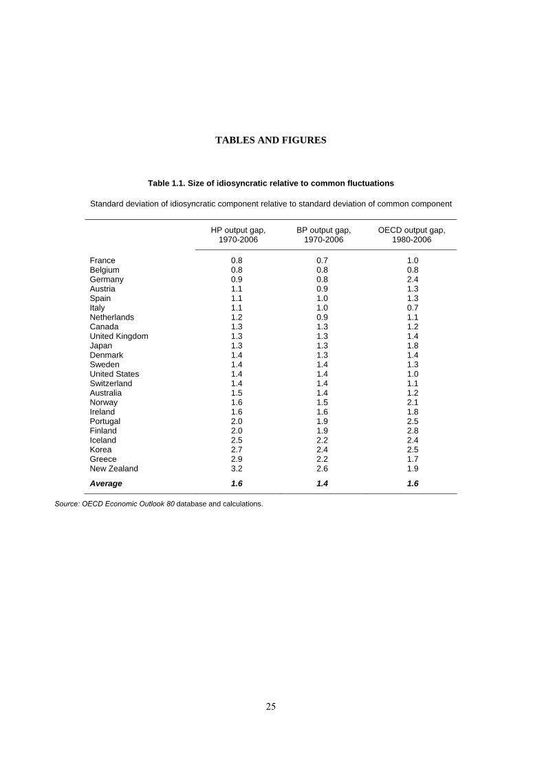
TABLES AND FIGURES

Table 1.1. Size of idiosyncratic relative to common fluctuations

Standard deviation of idiosyncratic component relative to standard deviation of common component

HP output gap, 1970-2006

BP output gap, 1970-2006

OECD output gap, 1980-2006

France 0.8 0.7 1.0 Belgium 0.8 0.8 0.8 Germany 0.9 0.8 2.4 Austria 1.1 0.9 1.3 Spain 1.1 1.0 1.3 Italy 1.1 1.0 0.7 Netherlands 1.2 0.9 1.1 Canada 1.3 1.3 1.2 United Kingdom 1.3 1.3 1.4 Japan 1.3 1.3 1.8 Denmark 1.4 1.3 1.4 Sweden 1.4 1.4 1.3 United States 1.4 1.4 1.0 Switzerland 1.4 1.4 1.1 Australia 1.5 1.4 1.2 Norway 1.6 1.5 2.1 Ireland 1.6 1.6 1.8 Portugal 2.0 1.9 2.5 Finland 2.0 1.9 2.8 Iceland 2.5 2.2 2.4 Korea 2.7 2.4 2.5 Greece 2.9 2.2 1.7 New Zealand 3.2 2.6 1.9

Average 1.6 1.4 1.6

Source: OECD Economic Outlook 80 database and calculations.

25

Table 1.2. Idiosyncratic relative to common fluctuations over time

Standard deviation of idiosyncratic component relative to standard deviation of common component

HP output gap BP output gap

1973-1989 1990-2006 1973-1989 1990-2006

France 0.7 0.8 0.7 0.7 Belgium 0.9 0.7 0.9 0.6 Germany 0.7 1.1 0.6 1.0 Austria 1.0 0.9 0.9 0.9 Spain 1.0 1.0 1.0 0.9 Italy 1.1 0.8 1.0 0.8 Netherlands 1.2 0.9 0.9 0.8 Canada 1.2 1.3 1.1 1.3 United Kingdom 1.4 1.0 1.3 1.0 Japan 1.1 1.4 1.0 1.5 Denmark 1.5 1.1 1.5 0.9 Sweden 1.5 1.0 1.4 1.0 United States 1.4 1.2 1.4 1.2 Switzerland 1.6 1.0 1.6 1.0 Australia 1.4 1.4 1.4 1.4 Norway 1.6 1.4 1.6 1.3 Ireland 1.5 1.8 1.6 1.5 Portugal 2.1 1.7 2.1 1.6 Finland 1.8 2.1 1.7 2.1 Iceland 1.9 2.8 2.0 2.2 Korea 2.3 3.3 2.3 3.4 Greece 3.2 2.1 2.4 1.2 New Zealand 3.4 2.1 2.7 2.0

Average 1.5 1.4 1.4 1.3

Source: OECD Economic Outlook 80 database and calculations.

Table 1.3. Idiosyncratic relative to common fluctuations in the euro area

Standard deviation of idiosyncratic component relative to standard deviation of common component

HP output gap BP output gap

1973-1989 1990-2006 1973-1989 1990-2006

France 0.5 0.5 0.3 0.3 Belgium 0.7 0.5 0.4 0.3 Germany 0.7 0.7 0.4 0.4 Austria 0.9 0.6 0.4 0.3 Spain 0.9 0.5 0.5 0.3 Italy 0.9 0.6 0.5 0.4 Netherlands 1.2 0.5 0.6 0.2 Ireland 1.3 1.2 0.7 0.6 Portugal 1.7 0.9 1.0 0.6 Finland 1.6 1.6 1.1 1.3 Greece 2.7 1.5 1.5 0.6

Average 1.2 0.8 0.7 0.5

Source: OECD Economic Outlook 80 database and calculations.

26

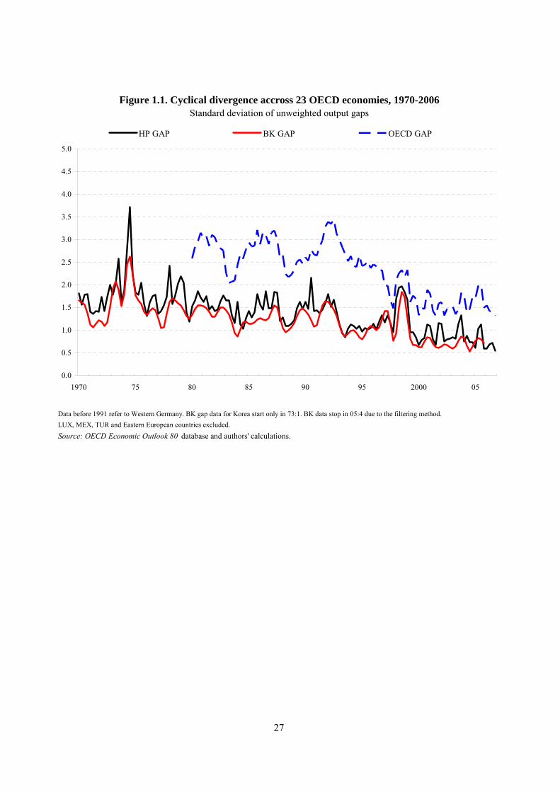
Data before 1991 refer to Western Germany. BK gap data for Korea start only in 73:1. BK data stop in 05:4 due to the filtering method. LUX, MEX, TUR and Eastern European countries excluded.Source: OECD Economic Outlook 80 database and authors' calculations.

Figure 1.1. Cyclical divergence accross 23 OECD economies, 1970-2006Standard deviation of unweighted output gaps

0.0

0.5

1.0

1.5

2.0

2.5

3.0

3.5

4.0

4.5

5.0

1970 75 80 85 90 95 2000 05

HP GAP BK GAP OECD GAP

27

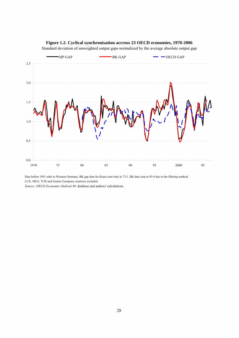
Data before 1991 refer to Western Germany. BK gap data for Korea start only in 73:1. BK data stop in 05:4 due to the filtering method. LUX, MEX, TUR and Eastern European countries excluded.Source: OECD Economic Outlook 80 database and authors' calculations.

Figure 1.2. Cyclical synchronisation accross 23 OECD economies, 1970-2006Standard deviation of unweighted output gaps normalized by the average absolute output gap

0.0

0.5

1.0

1.5

2.0

2.5

1970 75 80 85 90 95 2000 05

HP GAP BK GAP OECD GAP

28

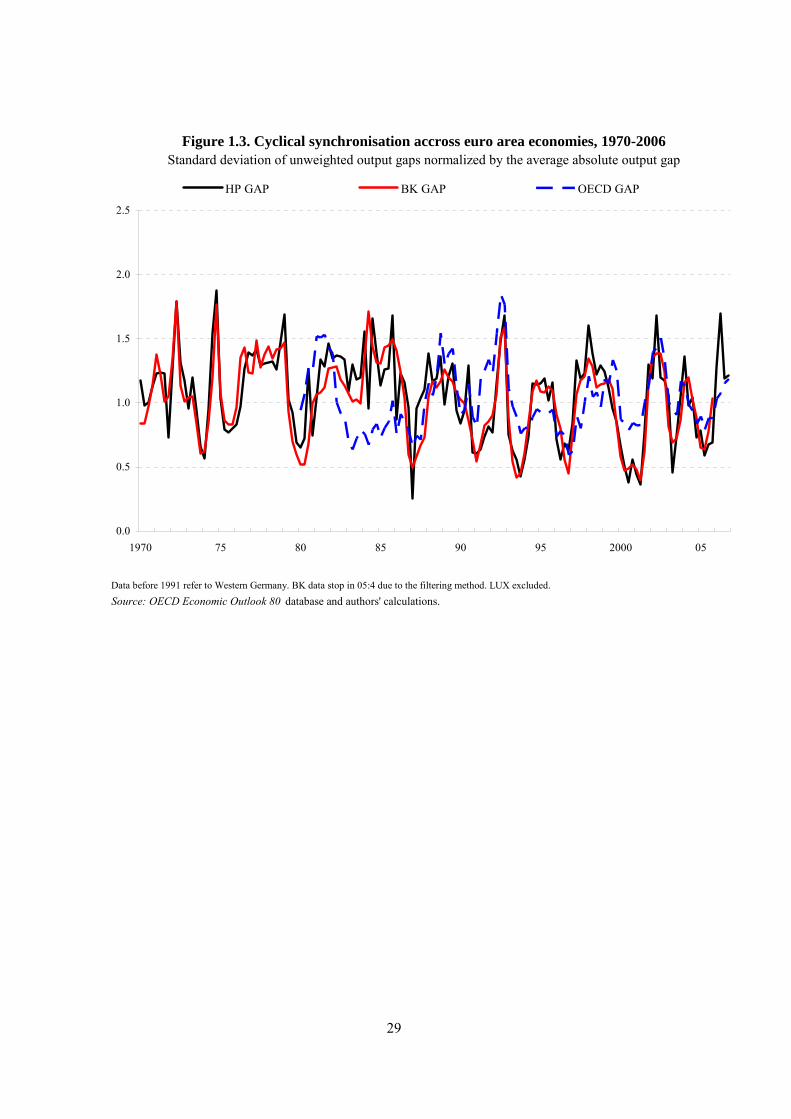
Data before 1991 refer to Western Germany. BK data stop in 05:4 due to the filtering method. LUX excluded.Source: OECD Economic Outlook 80 database and authors' calculations.

Figure 1.3. Cyclical synchronisation accross euro area economies, 1970-2006Standard deviation of unweighted output gaps normalized by the average absolute output gap

0.0

0.5

1.0

1.5

2.0

2.5

1970 75 80 85 90 95 2000 05

HP GAP BK GAP OECD GAP

29

LUX, MEX, TUR and Eastern European countries excluded.

Source: OECD Economic Outlook 80 database and authors' calculations.

B. 1990-2006

Figure 1.4. Cyclical correlation with the euro area average and the USCorrelation coefficient for quarterly HP output gaps

A. 1973-1989

Correlation with euro area

PRT

NLD

ITA

IRL

GRC

FRA

FIN

ESP

DEUBEL

AUT

USA

SWENZL NOR

KOR

JPN

ISL

GBR

DNK

CHE

CAN

AUS

-0.5

-0.4

-0.3

-0.2

-0.1

0.0

0.1

0.2

0.3

0.4

0.5

0.6

0.7

0.8

0.9

1.0

-0.5 -0.4 -0.3 -0.2 -0.1 0.0 0.1 0.2 0.3 0.4 0.5 0.6 0.7 0.8 0.9 1.0

Correlation with the US

Euro area countries Other OECD countries

Correlation with euro area

PRT

NLDITA

IRL

GRC

FRA

FIN

ESPDEU

BEL

AUT

USA

SWE

NZL

NORKOR

JPN

ISL GBR

DNK

CHE

CAN

AUS

-0.5

-0.4

-0.3

-0.2

-0.1

0.0

0.1

0.2

0.3

0.4

0.5

0.6

0.7

0.8

0.9

1.0

-0.5 -0.4 -0.3 -0.2 -0.1 0.0 0.1 0.2 0.3 0.4 0.5 0.6 0.7 0.8 0.9 1.0

Correlation with the US

Euro area countries Other OECD countries

30

Data before 1991 refer to Western Germany. BK gap data for Korea start only in 73:1.LUX, MEX, TUR and Eastern European countries excluded.Source: OECD Economic Outlook 80 database and authors' calculations.

Cycles are defined as lasting five quarters at least. Turning points require that the upturn or downturn lasts at least over two subsequent quarters.

Figure 1.5. Business cycle turning points accross 23 OECD economiesAverage number of turning points over current and previous three quarters

HP output gap measure

BK output gap measure

6

5

4

3

2

1

0

1

2

3

4

5

6

1970 75 80 85 90 95 2000 05

Peaks Troughs

6

5

4

3

2

1

0

1

2

3

4

5

6

1970 75 80 85 90 95 2000 05

Peaks Troughs

31

Data before 1991 refer to Western Germany. LUX eand SI excluded.Source: OECD Economic Outlook 80 database and authors' calculations.

BK output gap measure

Cycles are defined as lasting five quarters at least. Turning points require that the upturn or downturn lasts at least over two subsequent quarters.

Figure 1.6. Business cycle turning points accross euro membersAverage number of turning points over current and previous three quarters

HP output gap measure

3

2

1

0

1

2

3

1970 75 80 85 90 95 2000 05

Peaks Troughs

3

2

1

0

1

2

3

1970 75 80 85 90 95 2000 05

Peaks Troughs

32

Data before 1991 refer to Western Germany. BK gap data for Korea start only in 73:1. BK data stop in 05:4 due to the filtering method.LUX, MEX, TUR and Eastern European countries excluded. Source: OECD Economic Outlook 80 database and authors' calculations.

B. Across 11 euro area countries

Figure 1.7. Common components in business cycles accross countriesSum of the intercept plus time dummies from a regression of output gaps on time and country dummies only.

A. Across 23 OECD countries

-5

-4

-3

-2

-1

0

1

2

3

4

5

1970 75 80 85 90 95 2000 05

HP GAP BK GAP OECD GAP

-5

-4

-3

-2

-1

0

1

2

3

4

5

1970 75 80 85 90 95 2000 05

HP GAP BK GAP OECD GAP

33

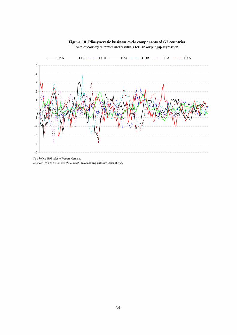
Data before 1991 refer to Western Germany.Source: OECD Economic Outlook 80 database and authors' calculations.

Figure 1.8. Idiosyncratic business cycle components of G7 countriesSum of country dummies and residuals for HP output gap regression

-5

-4

-3

-2

-1

0

1

2

3

4

5

1970 75 80 85 90 95 2000 05

USA JAP DEU FRA GBR ITA CAN

34

Persistence of shocks:1

coefficientImplied half-life of output gaps

(in years)

Amplification of shocks:1

coefficient

Estimate for the US:

USA 0.44 1.67 0.41

Estimates for other OECD countriesand test for statistical differences in coefficients with respect to the US:

AUS 0.34 1.3 0.24* *

AUT 0.47 1.8 -0.85***

BEL 0.45 1.7 -0.25*

CAN 0.27 1.1 0.34** **

CHE 0.41 1.6 -0.16*

DEU1 0.42 1.6 -0.15

DNK 0.31 1.2 -0.49* * **

ESP 0.54 2.3 -0.41** ** **

FIN1 0.49 2.0 0.24

FRA 0.50 2.0 -0.53***

GBR 0.41 1.6 -0.30*

IRL 0.49 1.9 0.37

ITA 0.47 1.9 -0.37**

JPN 0.50 2.0 -0.57***

NLD 0.50 2.0 -0.55**

NOR 0.57 2.5 -0.97*** *** ***

NZL 0.38 1.4 -0.61***

PRT 0.56 2.4 -0.38*** *** **

SWE1 0.40 1.5 0.18

Time dummies yesObservations 434

R-squared 0.85Non-linear least squares.* (**, ***): estimated coefficient differs significantly from corresponding coefficient obtained for the US at the 10% (5%, 1%) level.1. (weighted) average over periods 1982-1990 and 1993-2003.Source : Authors' estimates.

Table 2.1. Output gap equations with country dummies (20 OECD countries, 1982-2003)

iηϕ iγ

35

Persistence of shocks: coefficient Amplification of shocks: coefficient

Benefit replacement rate 0.12 -0.39*

EPL for regular contracts 0.62*** -0.43**

PMR 0.58*** -0.46**

Collective bargaining coverage 0.29 -0.23

Low corporatism -0.52*** 0.54***

Labour and product market regulation(synthetic indicator) 0.5** -0.51**

Source : Authors' estimates on the basis of country-specific persistence and amplification coefficients estimated in Table 2.1 and data sources described in the data appendix.

coefficients and labour/product market policy indicatorsTable 2.2. Cross-country correlation coefficients between persistence/amplification

(based on simpleregressions of country-specific coefficients on the average value of each policy indicator over the period 1982-2003, using bootstrapped critical values to assess statistical significance)

iγiϕ

36

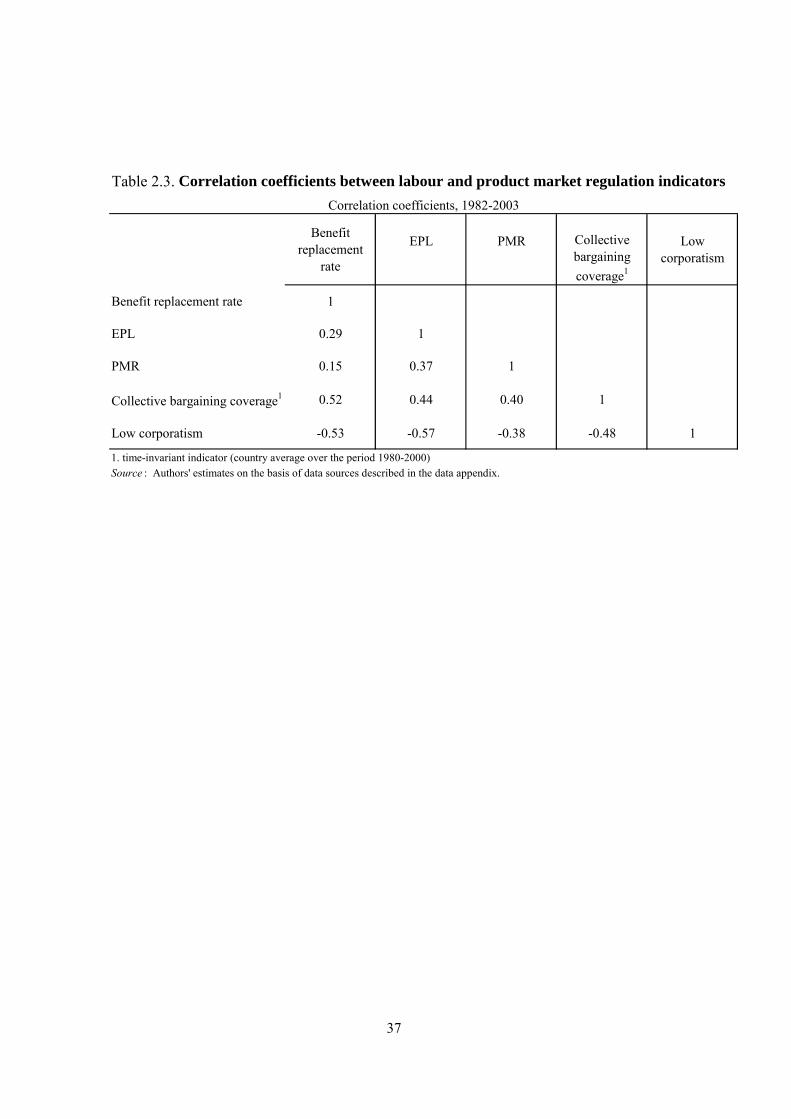
Table 2.3. Correlation coefficients between labour and product market regulation indicators

Benefit replacement

rate

EPL PMR Collective bargaining coverage1

Low corporatism

Benefit replacement rate 1

EPL 0.29 1

PMR 0.15 0.37 1

Collective bargaining coverage1 0.52 0.44 0.40 1

Low corporatism -0.53 -0.57 -0.38 -0.48 1

1. time-invariant indicator (country average over the period 1980-2000)Source : Authors' estimates on the basis of data sources described in the data appendix.

Correlation coefficients, 1982-2003

37

1 2 3 4 5 6 7

Benefitreplacement

rate

EPL Low corporatism

Bargaining coverage

PMRFinal model

selected from statistical

tournament

Full model with all policies and

institutions

Persistence coefficients:1.077 1.081 1.069 1.123 1.112 1.085 1.113

[22.96]*** [24.71]*** [23.54]*** [23.98]*** [25.46]*** [24.96]*** [20.71]***0.395 0.425 0.390 0.393 0.399 0.425 0.418

[9.62]*** [11.19]*** [9.55]*** [9.68]*** [10.27]*** [11.39]*** [10.41]***

Effect of institutions on persistence:

Benefit replacement rate 0.002 -0.004[0.75] [1.23]

EPL 0.141 0.128 0.106[5.11]*** [4.77]*** [3.01]***

Low corporatism -0.279 -0.070[3.40]*** [0.69]

Collective bargaining coverage 0.004 0.002[2.63]*** [1.11]

PMR 0.099 0.025[3.15]*** [0.68]

Effect of institutions on amplification of shocks:

Benefit replacement rate -0.007 0.002[1.09] [0.33]

EPL -0.242 -0.088[2.93]*** [0.89]

Low corporatism 0.493 0.364[2.47]** [1.47]

Collective bargaining coverage -0.002 0.005[0.51] [1.22]

PMR -0.508 -0.537 -0.431[6.15]*** [5.93]*** [4.15]***

Country fixed effects yes yes yes yes yes yes yesTimes dummies yes yes yes yes yes yes yesObservations 434 434 434 434 434 434 434R-squared 0.82 0.83 0.82 0.82 0.83 0.83 0.84Non-linear least squares. Absolute value of t statistics in brackets.* significant at 10%; ** significant at 5%; *** significant at 1%.Source : Authors' estimates.

Table 2.4. Output gap equations with labour and product market regulation indicators (20 OECD countries, 1982-2003)

kγ

φ

jϕ

η

38

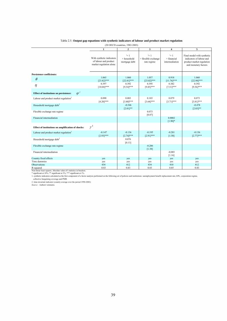
1 2 3 4 5

With synthetic indicators of labour and product

market regulation alone

'= 1 + household

mortgage debt

'= 1 + flexible exchange

rate regime

'= 1 + financial

intermediation

Final model with synthetic indicators of labour and

product market regulation and monetary factors

Persistence coefficients:1.065 1.060 1.057 0.918 1.060

[23.82]*** [22.81]*** [23.02]*** [11.76]*** [22.98]***0.397 0.392 0.395 0.382 0.392

[10.04]*** [9.54]*** [9.85]*** [7.51]*** [9.56]***

Effect of institutions on persistence:

Labour and product market regulation1 0.090 0.083 0.103 0.079 0.073[4.20]*** [3.80]*** [3.64]*** [3.71]*** [3.81]***

Household mortgage debt2 -0.546 -0.478[2.01]** [2.03]**

Flexible exchange rate regime 0.073[0.87]

Financial intermediation 0.0002[1.90]*

Effect of institutions on amplification of shocks:

Labour and product market regulation1 -0.147 -0.136 -0.195 -0.281 -0.136[2.93]*** [2.74]*** [2.91]*** [1.50] [2.77]***

Household mortgage debt2 0.076[0.13]

Flexible exchange rate regime -0.286[1.38]

Financial intermediation -0.003[1.16]

Country fixed effects yes yes yes yes yesTime dummies yes yes yes yes yesObservations 434 412 434 410 412R-squared 0.83 0.83 0.83 0.85 0.83Non-linear least squares. Absolute value of t statistics in brackets.* significant at 10%; ** significant at 5%; *** significant at 1%.1. synthetic indicators calculated as the first component of a factor analysis performed on the following set of policies and institutions: unemployment benefit replacement rate, EPL, corporatism regime, collective bargaining coverage and PMR.2. time-invariant indicator (country average over the period 1990-2002)Source : Authors' estimates.

Table 2.5. Output gap equations with synthetic indicators of labour and product market regulation(20 OECD countries, 1982-2003)

jϕ

kγ

φ

η

39

Persistence of shocks:coefficient ξ i

Amplification of shocks:coefficient ξi

Household mortgage debt -0.38* 0.03

Intermediation of financial system 0.36* 0.11

Flexible exchange rate regime -0.43** 0.32

Source : Authors' estimates on the basis of country-specific persistence and amplification coefficients estimated in Table 2.1 and data sources described in the data appendix.

coefficients and monetary/financial variablesTable 2.6. Correlation coefficients between country-specific persistence/amplification

based on simpleregressions of country-specific coefficients on the average value of each indicator over the period 1982-2003, using bootstrapped critical values to assess statistical significance)

40

1 2Full model

with all policies and institutions(dependent variable: unemployment rate)

Final model selected after dropping insignificant variables

(dependent variable: unemployment rate)

Policies and institutions:Benefit replacement rate 0.064 0.072

[3.11]*** [4.14]***Labour tax wedge 0.142 0.139

[5.20]*** [5.12]***High corporatism -1.203 -1.590

[2.89]*** [4.11]***PMR 0.711 0.661

[6.31]*** [8.97]***Union density -0.031

[1.36]EPL 0.259

[0.85]

Cyclical controls:

GDP growth (t) -0.164 -0.150[4.14]*** [3.74]***

GDP growth (t-1) -0.305 -0.300[7.33]*** [7.19]***

GDP growth (t-2) -0.246 -0.237[6.02]*** [5.68]***

GDP growth (t-3) -0.256 -0.252[6.26]*** [6.10]***

GDP growth (t-4) -0.139 -0.131[3.15]*** [2.81]***

GDP growth (t-5) -0.134 -0.132[4.04]*** [3.84]***

GDP growth (t-6) -0.129 -0.123[3.73]*** [3.53]***

Country fixed effects yes yesTime dummies no noObservations 434 434R-squared 0.98 0.98Ordinary least squares (Within estimates). Absolute value of t statistics in brackets.* significant at 10%; ** significant at 5%; *** significant at 1%.Source : Authors' estimates based on Bassanini and Duval (2006).

Table 2.7. Structural unemployment econometric estimates (20 OECD countries, 1982-2003)

41

1 2 3

Model selected from statistical tournament

Model with synthetic indicators of labour and product market

regulation alone

Model with synthetic indicators of labour and product market

regulation and monetary factors

Persistence coefficients:0.995 0.983 0.975

[22.75]*** [22.08]*** [21.09]***0.430 0.408 0.394

[10.43]*** [9.52]*** [8.88]***

Effect of institutions on persistence:

Labour and product market regulation2 0.094 0.090[4.14]*** [3.86]***

Household mortgage debt2 -0.658[2.36]**

EPL 0.145[4.84]***

Effect of institutions on amplification of shocks:

Labour and product market regulation2 -0.127 -0.126[2.76]*** [2.80]***

Household mortgage debt3

PMR -0.452[5.90]***

Country fixed effects yes yes yesTime dummies yes yes yesObservations 431 431 409R-squared 0.81 0.80 0.80Non-linear least squares. Absolute value of t statistics in brackets.* significant at 10%; ** significant at 5%; *** significant at 1%.1. See Section 1.1 in the main text for the definition of the Hodrick-Prescott-filtered output gap.2. synthetic indicators calculated as the first component of a factor analysis performed on the following set of policies and institutions: unemployment benefit replacement rate, EPL, corporatism regime, collective bargaining coverage and PMR.3. time-invariant indicator (country average over the period 1990-2002)Source : Authors' estimates.

Table 2.8. Equations with alternative output gap definitions: Hodrick-Prescott filter gap1 estimates (20 OECD countries, 1982-2003)

η

φ

jϕ

kγ

42

1 2 3

Model selected from statistical tournament

Model with synthetic indicators of labour and product market

regulation alone

Model with synthetic indicators of labour and product market

regulation and monetary factors

Persistence coefficients:0.551 0.541 0.541

[12.10]*** [11.69]*** [11.18]***0.480 0.439 0.428

[6.44]*** [5.49]*** [5.21]***

Effect of institutions on persistence:

Labour and product market regulation2 0.112 0.116[3.94]*** [3.90]***

Household mortgage debt2 0.019[0.06]

EPL 0.213[5.00]***

Effect of institutions on amplification of shocks:

Labour and product market regulation2 -0.121 -0.122[2.67]*** [2.61]***

Household mortgage debt3

PMR -0.427[5.61]***

Country fixed effects yes yes yesTime dummies yes yes yesObservations 431 431 409R-squared 0.59 0.58 0.57Non-linear least squares. Absolute value of t statistics in brackets.* significant at 10%; ** significant at 5%; *** significant at 1%.1. See Section 1.1 in the main text for the definition of the Baxter-King filtered output gap.2. synthetic indicators calculated as the first component of a factor analysis performed on the following set of policies and institutions: unemployment benefit replacement rate, EPL, corporatism regime, collective bargaining coverage and PMR.3. time-invariant indicator (country average over the period 1990-2002)Source : Authors' estimates.

Table 2.8. (cont.) Equations with alternative output gap definitions: Baxter-King filter gap1 estimates (20 OECD countries, 1982-2003)

η

φ

jϕ

kγ

43

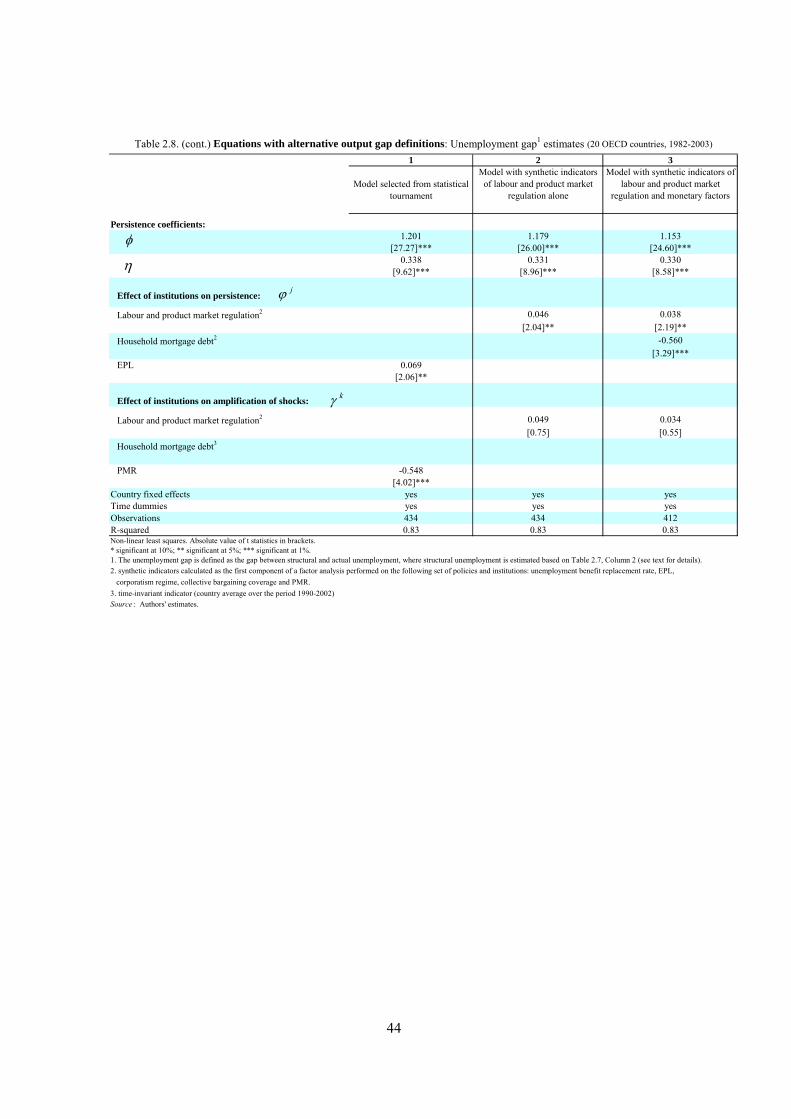
1 2 3

Model selected from statistical tournament

Model with synthetic indicators of labour and product market

regulation alone

Model with synthetic indicators of labour and product market

regulation and monetary factors

Persistence coefficients:1.201 1.179 1.153

[27.27]*** [26.00]*** [24.60]***0.338 0.331 0.330

[9.62]*** [8.96]*** [8.58]***

Effect of institutions on persistence:

Labour and product market regulation2 0.046 0.038[2.04]** [2.19]**

Household mortgage debt2 -0.560[3.29]***

EPL 0.069[2.06]**

Effect of institutions on amplification of shocks:

Labour and product market regulation2 0.049 0.034[0.75] [0.55]

Household mortgage debt3

PMR -0.548[4.02]***

Country fixed effects yes yes yesTime dummies yes yes yesObservations 434 434 412R-squared 0.83 0.83 0.83Non-linear least squares. Absolute value of t statistics in brackets.* significant at 10%; ** significant at 5%; *** significant at 1%.1. The unemployment gap is defined as the gap between structural and actual unemployment, where structural unemployment is estimated based on Table 2.7, Column 2 (see text for details).2. synthetic indicators calculated as the first component of a factor analysis performed on the following set of policies and institutions: unemployment benefit replacement rate, EPL, corporatism regime, collective bargaining coverage and PMR.3. time-invariant indicator (country average over the period 1990-2002)Source : Authors' estimates.

Table 2.8. (cont.) Equations with alternative output gap definitions: Unemployment gap1 estimates (20 OECD countries, 1982-2003)

η

φ

jϕ

kγ

44

1 2 3

Model selected from statistical tournament

Model with synthetic indicators of labour and product market

regulation alone

Model with synthetic indicators of labour and product market

regulation and monetary factors

Persistence coefficients:1.203 1.229 1.221

[35.54]*** [36.87]*** [34.85]***0.277 0.278 0.271

[10.38]*** [10.64]*** [9.76]***

Effect of institutions on persistence:

Labour and product market regulation1 0.028 0.029[2.07]** [2.05]**

Household mortgage debt2 -0.322[1.80]*

EPL 0.066[3.72]***

Effect of institutions on amplification of shocks:

Labour and product market regulation1 -0.070 -0.063[2.96]*** [2.60]***

Household mortgage debt2

PMR -0.074[2.06]**

Country fixed effects yes yes yesTime dummies yes yes yesObservations 394 394 376R-squared 0.92 0.92 0.92Non-linear least squares. Absolute value of t statistics in brackets.* significant at 10%; ** significant at 5%; *** significant at 1%.1. synthetic indicators calculated as the first component of a factor analysis performed on the following set of policies and institutions: unemployment benefit replacement rate, EPL, corporatism regime, collective bargaining coverage and PMR.2. time-invariant indicator (country average over the period 1990-2002)Source : Authors' estimates.

Table 2.9. Output gap equations with both observed and unobserved shocks (20 OECD countries, 1982-2003)

η

φ

jϕ

kγ

45

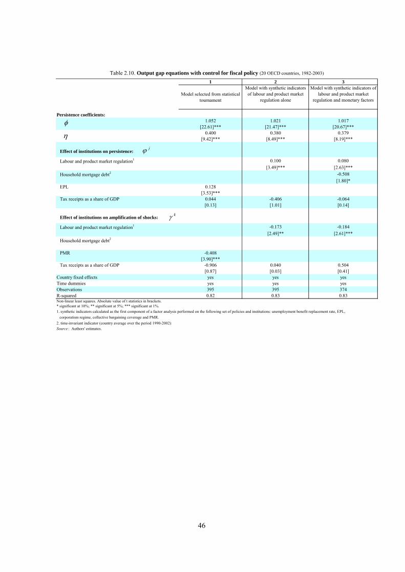
1 2 3

Model selected from statistical tournament

Model with synthetic indicators of labour and product market

regulation alone

Model with synthetic indicators of labour and product market

regulation and monetary factors

Persistence coefficients:1.052 1.021 1.017

[22.61]*** [21.47]*** [20.67]***0.400 0.380 0.379

[9.42]*** [8.49]*** [8.19]***

Effect of institutions on persistence:

Labour and product market regulation1 0.100 0.080[3.49]*** [2.63]***

Household mortgage debt2 -0.508[1.80]*

EPL 0.128[3.53]***

Tax receipts as a share of GDP 0.044 -0.406 -0.064[0.13] [1.01] [0.14]

Effect of institutions on amplification of shocks:

Labour and product market regulation1 -0.173 -0.184[2.49]** [2.61]***

Household mortgage debt2

PMR -0.408[3.90]***

Tax receipts as a share of GDP -0.906 0.040 0.504[0.87] [0.03] [0.41]

Country fixed effects yes yes yesTime dummies yes yes yesObservations 395 395 374R-squared 0.82 0.83 0.83Non-linear least squares. Absolute value of t statistics in brackets.* significant at 10%; ** significant at 5%; *** significant at 1%.1. synthetic indicators calculated as the first component of a factor analysis performed on the following set of policies and institutions: unemployment benefit replacement rate, EPL, corporatism regime, collective bargaining coverage and PMR.2. time-invariant indicator (country average over the period 1990-2002)Source : Authors' estimates.

Table 2.10. Output gap equations with control for fiscal policy (20 OECD countries, 1982-2003)

η

φ

jϕ

kγ

46

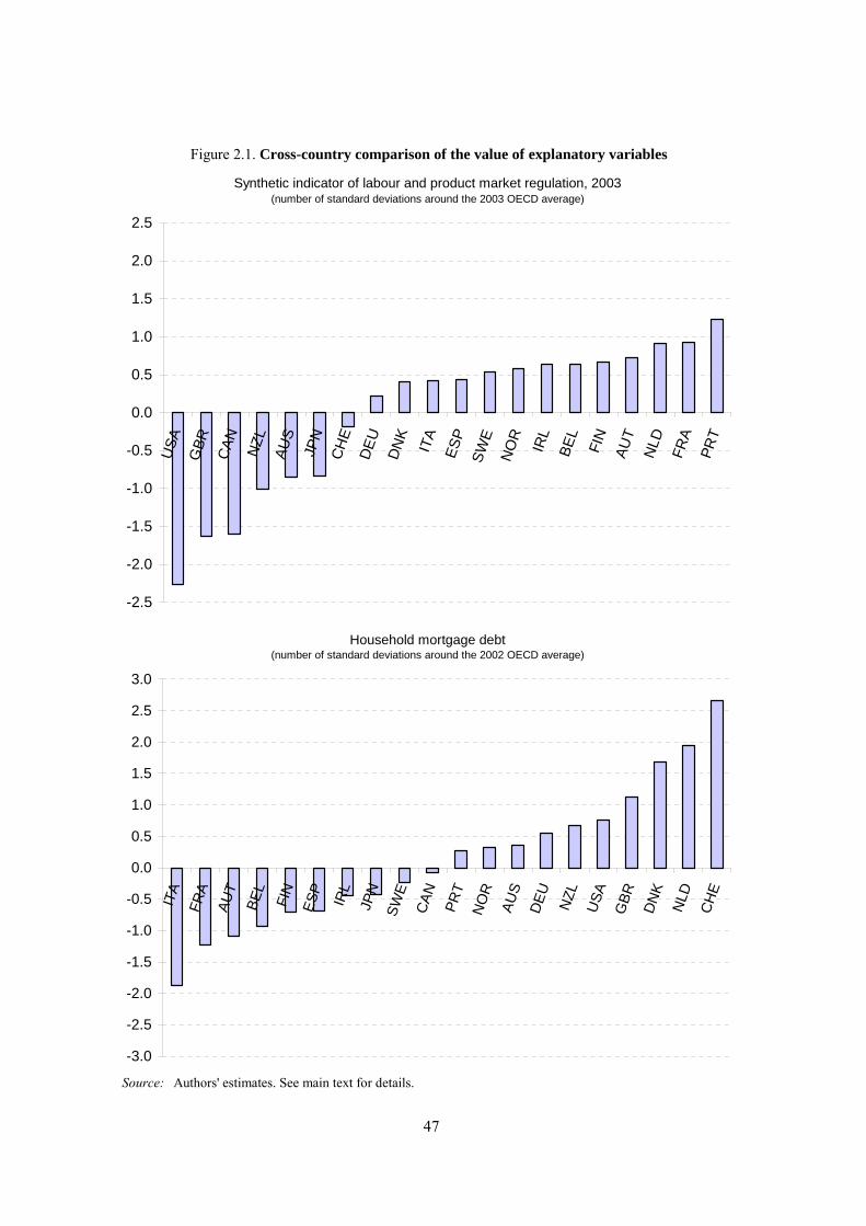
Source: Authors' estimates. See main text for details.

Figure 2.1. Cross-country comparison of the value of explanatory variables

-2.5

-2.0

-1.5

-1.0

-0.5

0.0

0.5

1.0

1.5

2.0

2.5

USA

GBR

CAN NZL

AUS

JPN

CH

ED

EUD

NK

ITA

ESP

SWE

NO

RIR

LBE

LFI

NAU

TN

LDFR

APR

T

Synthetic indicator of labour and product market regulation, 2003(number of standard deviations around the 2003 OECD average)

-3.0

-2.5

-2.0

-1.5

-1.0

-0.5

0.0

0.5

1.0

1.5

2.0

2.5

3.0

ITA

FRA

AUT

BEL

FIN

ESP

IRL

JPN

SWE

CAN PR

TN

OR

AUS

DEU NZL

USA

GBR

DN

KN

LDC

HE

Household mortgage debt(number of standard deviations around the 2002 OECD average)

47

Source: Authors' estimates. See main text for details.

(assuming a 1 percentage point common negative shock to the output gap, based on Table 2.4, column 5)Figure 2.2. Impulse-response functions

Canada

-1.6

-1.2

-0.8

-0.4

0.0

0.4

0 1 2 3 4 5 6 7 8 9 10

years

output gap France

-1.6

-1.2

-0.8

-0.4

0.0

0.4

0 1 2 3 4 5 6 7 8 9 1

years

output gap

0

Germany

-1.6

-1.2

-0.8

-0.4

0.0

0.4

0 1 2 3 4 5 6 7 8 9 10

output gap

years

Italy

-1.6

-1.2

-0.8

-0.4

0.0

0.4

0 1 2 3 4 5 6 7 8 9 1

output gap

years

0

Japan

-1.6

-1.2

-0.8

-0.4

0.0

0.4

0 1 2 3 4 5 6 7 8 9 10

output gap

years

Spain

-1.6

-1.2

-0.8

-0.4

0.0

0.4

0 1 2 3 4 5 6 7 8 9 1

output gap

years

0

United Kingdom

-1.6

-1.2

-0.8

-0.4

0.0

0.4

0 1 2 3 4 5 6 7 8 9 10

output gap

years

United States

-1.6

-1.2

-0.8

-0.4

0.0

0.4

0 1 2 3 4 5 6 7 8 9 1

output gap

years

0

48

Source: Authors' estimates. See main text for details.

Figure 2.2 (continued). Impulse-response functions(assuming a 1 percentage point common negative shock to the output gap, based on Table 2.4, column 5)

Australia

-1.6

-1.2

-0.8

-0.4

0.0

0.4

0 1 2 3 4 5 6 7 8 9 10

output gap Belgium

-1.6

-1.2

-0.8

-0.4

0.0

0.4

0 1 2 3 4 5 6 7 8 9 1

output gap

0

Denmark

-1.6

-1.2

-0.8

-0.4

0.0

0.4

0 1 2 3 4 5 6 7 8 9 10

output gap

years

Ireland

-1.6

-1.2

-0.8

-0.4

0.0

0.4

0 1 2 3 4 5 6 7 8 9 1

output gap

years

0

New Zealand

-1.6

-1.2

-0.8

-0.4

0.0

0.4

0 1 2 3 4 5 6 7 8 9 10

output gap

years

Norway

-1.6

-1.2

-0.8

-0.4

0.0

0.4

0 1 2 3 4 5 6 7 8 9 1

output gap

years

0

Portugal

-1.6

-1.2

-0.8

-0.4

0.0

0.4

0 1 2 3 4 5 6 7 8 9 10

output gap

years

Sweden

-1.6

-1.2

-0.8

-0.4

0.0

0.4

0 1 2 3 4 5 6 7 8 9 1

output gap

years

0

49

Source: Authors' estimates. See main text for details.

Figure 2.2 (continued). Impulse-response functions(assuming a 1 percentage point common negative shock to the output gap, based on Table 2.4, column 5)

Austria

-1.6

-1.2

-0.8

-0.4

0.0

0.4

0 1 2 3 4 5 6 7 8 9 10

output gap

years

Finland

-1.6

-1.2

-0.8

-0.4

0.0

0.4

0 1 2 3 4 5 6 7 8 9 1

output gap

years

0

Netherlands

-1.6

-1.2

-0.8

-0.4

0.0

0.4

0 1 2 3 4 5 6 7 8 9 10

output gap

years

Switzerland

-1.6

-1.2

-0.8

-0.4

0.0

0.4

0 1 2 3 4 5 6 7 8 9 1

output gap

years

0

50

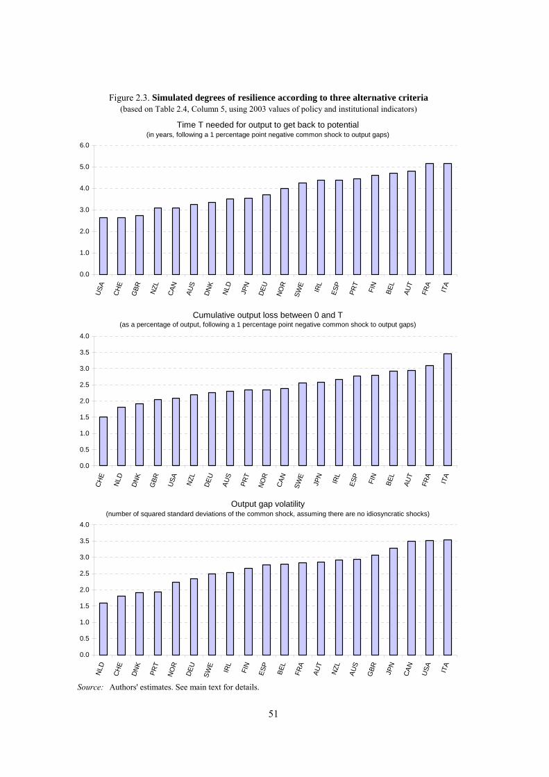
Source: Authors' estimates. See main text for details.

Figure 2.3. Simulated degrees of resilience according to three alternative criteria(based on Table 2.4, Column 5, using 2003 values of policy and institutional indicators)

0.0

0.5

1.0

1.5

2.0

2.5

3.0

3.5

4.0

NLD

CH

E

DN

K

PRT

NO

R

DEU

SWE

IRL

FIN

ESP

BEL

FRA

AUT

NZL

AUS

GBR JP

N

CAN USA IT

A

Output gap volatility(number of squared standard deviations of the common shock, assuming there are no idiosyncratic shocks)

0.0

1.0

2.0

3.0

4.0

5.0

6.0

USA

CH

E

GBR NZL

CAN AU

S

DN

K

NLD JPN

DEU

NO

R

SWE

IRL

ESP

PRT

FIN

BEL

AUT

FRA

ITA

Time T needed for output to get back to potential(in years, following a 1 percentage point negative common shock to output gaps)

0.0

0.5

1.0

1.5

2.0

2.5

3.0

3.5

4.0

CH

E

NLD

DN

K

GBR USA NZL

DEU AU

S

PRT

NO

R

CAN

SWE

JPN

IRL

ESP

FIN

BEL

AUT

FRA

ITA

Cumulative output loss between 0 and T(as a percentage of output, following a 1 percentage point negative common shock to output gaps)

51

DATA APPENDIX: DATA SOURCES AND METHODOLOGY

OECD measure of the output gap:

Definition: OECD measure of the gap between actual and potential output as a percentage of potential output, in %. The methodology followed by the OECD in order to estimate output gaps is based on a Cobb-Douglas production function with Harrod-neutral technological progress and is described in detail in Giorno et al. (1995). The approach may best be qualified as hybrid in the sense that it relies on both structural economic relationships to estimate NAIRUs (see Richardson et al., 2000) -- and univariate filters -- mostly HP filters, to estimate trend participation rates, trend hours worked and trend total factor productivity.

Source: OECD, Economic Outlook 78, December 2005.

Aggregate unemployment rate:

Definition: unemployed workers as share of the labour force, in %.

Source: OECD, Database on Labour Force Statistics; OECD, Annual Labour Force Statistics.

Data adjustments: while the primary source is the OECD Database on Labour Force Statistics, Annual Labour Force Statistics -- which are usually available over longer time periods -- were also used in some cases to extrapolate unemployment rates backwards (under the assumption of similar percentage changes in unemployment rates in both sources).

Unemployment benefit replacement rate:

Definition: average unemployment benefit replacement rate across two income situations (100% and 67% of average production worker (APW) earnings), three family situations (single, with dependent spouse, with spouse in work) and three different unemployment durations (1st year, 2nd and 3rd years, and 4th and 5th years of unemployment).

Source: OECD, Benefits and Wages.

Data adjustments: original data are available only for odd years. Data for even years are obtained by linear interpolation.

Employment Protection Legislation (EPL):

Definition: OECD summary indicator of the stringency of Employment Protection Legislation.

Source: OECD, Employment Outlook 2004.

52

Product Market Regulation (PMR):

Definition: OECD summary indicator of regulatory impediments to product market competition in seven non-manufacturing industries39: gas, electricity, post, telecoms (mobile and fixed services), passenger air transport, railways (passenger and freight services) and road freight.

Source: Conway, P. and G. Nicoletti (2006) “Product Market Regulation in the Non-Manufacturing Sectors of OECD Countries: Measurement and Highlights”, Economics Department Working Paper No. 530.

Degree of corporatism:

Definition: indicator of the degree of centralisation/co-ordination of the wage bargaining processes, which takes values 1 for decentralised and uncoordinated processes, and 2 and 3 for intermediate and high degrees of centralisation/co-ordination, respectively. The “low corporatism” dummy variable frequently used in this paper equals 1 when bargaining is decentralised and uncoordinated and 0 otherwise. The “high corporatism” dummy variable used in structural unemployment regressions equals 1 when bargaining is highly centralised and/or co-ordinated and 0 otherwise.

Source: OECD, Employment Outlook 2004.

Data adjustments: original data are five-year averages and classify countries in each period along a 0-5 scale from least to most “corporatist” countries. In the present paper, annual data have been reconstructed based on various sources on the timing of past changes in centralisation and/or co-ordination of wage bargaining. Furthermore, the indicator has been rescaled along a 1-3 scale. In this process, it has been assumed that wage bargaining in France predominantly occurs at the intermediate level, while original data describe it as a mix of firm-level and industry-level bargaining. For other countries, values 1, 2 and 3 correspond to values 1-2, 3 and 4-5 in the original dataset, respectively.

Collective bargaining coverage:

Definition: share of workers covered by a collective agreement, in %. The variable used in the econometric estimates is the country average computed over the period 1980-2000.

Source: OECD, Employment Outlook 2004. In the case of Ireland, the average bargaining coverage rate is taken from Belot, M. and J. Van Ours (2004).

Union density:

Definition: trade union density rate, i.e. the share of workers affiliated to a trade union, in %.

Source: OECD, Employment Outlook 2004.

Data adjustments: data for missing years are obtained by linear interpolation. Furthermore, original data are typically available until 2001 for most OECD countries. Extrapolations have therefore been made in order to expand data availability up to 2003. These are mainly based on national sources but, in some 39. Details on the broader PMR indicator for the whole economy -- which is available only over the period

1998-2003 and therefore is not used in this paper -- can be found in Conway, P., V. Janod and G. Nicoletti (2005), “Product Market Regulation in OECD Countries: 1998 to 2003”, OECD Economics Department Working Paper No. 41.

53

cases, an assumption of unchanged union densities over the period 2001-03 had to be made due to lack of data.

Labour tax wedge:

Definition: tax wedge between the labour cost to the employer and the corresponding net take-home pay of the employee for a single-earner couple with two children earning 100% of APW earnings. The tax wedge corresponds to the sum of personal income tax and all social security contributions as a percentage of total labour cost.

Source: OECD, Taxing Wages.

Data adjustments: Austria: original data includes employers’ social security contributions starting from 1997 only, thereby inducing an upward shift in tax wedge from this year; the tax wedge starting from 1997 is therefore recalculated based on the fact that employers’ contribution rates to social security remained unchanged between 1996 and 1997. Netherlands: unlike other years, in 2002 and 2003 APW earnings are just above the threshold beyond which employers and employees do no longer have to contribute to the national health insurance plan (private medical insurance is typically provided instead), thereby inducing a temporary decline in the tax wedge; this issue is addressed by replacing the 2002 and 2003 observations by data obtained from linear interpolations between the 2001 and 2004 observations.

Monetary policy autonomy:

Definition: dummy variable which equals 1 when a country’s (de jure) exchange rate regime is “floating” or “floating with discretionary intervention” and 0 otherwise.

Source: These data represent the de jure classification of IMF countries’ exchange rate regimes, as collected and normalized by Ghosh, A., A-M. Gulde and H. Wolf, Exchange Rate Regimes: Choices and Consequences, The MIT Press, Cambridge, Massachussets, 2002.

Household mortgage debt:

Definition: Household mortgage debt as a share of GDP, in %. The variable used in the econometric estimates is the country average computed over the period 1990-2002. In the absence of available data for Switzerland before 2000, this country is excluded from all those regressions that include household mortgage debt among the set of explanatory variables. However, it is included in the illustrative impulse-response functions that are produced using the estimated regressions.

Source: Catte, P. et al. (2004) and, for Switzerland, Swiss National Bank (2004), Swiss Financial Accounts.

Financial intermediation:

Definition: Ratio of private credit by deposit money banks and other financial institutions to total stock market value traded -- which is the value of the trades of domestic shares on domestic exchanges.

Source: World Bank, Financial Structure Database.

54

Total factor productivity shock:

Definition: deviation of the logarithm of Total Factor Productivity (TFP) from its trend calculated by means of a Hodrick-Prescott (HP) filter (smoothing parameter λ = 100). The calculation proceeds in three steps. First, growth in the Solow residual in the business sector is calculated as:

ααα /)]log()1()log()log([)log( KNYTFP ∆−+∆−∆=∆ , where Y refers to real business sector GDP, N to total employment, K to the gross capital stock and α to labour income as a share of business sector income. Second, an index log(TFP) of the logarithm of TFP is obtained by cumulating the annual values of ∆log(TFP). Finally, the TFP shock variable is computed as the difference between log(TFP) and its HP filtered trend.

Source: Bassanini and Duval (2006), Annex 2.

Terms of trade shock:

Definition: logarithm of the relative price of imports weighted by the share of imports in GDP, i.e. terms of trade shock = (M/Y) * log(PM / PY), where M and Y denote total imports and GDP in nominal terms, respectively, and (PM / PY) is the ratio of the deflator of total imports to the GDP deflator.

Source: Bassanini and Duval (2006), Annex 2.

Real interest shock:

Definition: difference between the 10-year nominal US government bond yield (in %) and the annual change in the US GDP deflator (in %).

Source: Bassanini and Duval (2006), Annex 2.

Labour demand shocks:

Definition: logarithm of the labour share in business sector GDP purged from the short-run influence of factor prices.

The methodology follows Blanchard O. and J. Wolfers (2000). First, measures of real wages and employment in efficiency units are computed as Wefficiency units = (W / PY) / TFP and Nefficiency units = N * TFP, respectively. The simplest possible measure of labour demand shocks would be the negative of the sum of the logarithm of the ratio of labour input in efficiency units to real output in the business sector, on the one hand, and the logarithm of real wages in efficiency units, on the other hand: – [log(Nefficiency units / Y) + log(Wefficiency units)] = – log[(N * TFP) / Y] – log[(W / PY) / TFP] = –log [(W * N) / (PY * Y)] = – (labour’s share of business sector income). However, this simple measure of labour demand shocks is accurate only to the extent that the production function is Cobb-Douglas and factor proportions adjust instantaneously to changes in factor prices. Insofar as the latter assumption is unlikely to be verified in the short-run, changes in the labour share reflect both genuine labour demand shocks and the lagged adjustment of factor proportions to changes in factor prices.

Therefore, it is necessary to purge the labour share from the short-run influence of factor prices. For simplicity and comparative purposes, this is done here by following the same methodology as Blanchard (1998). Concretely, a wage measure which takes into account the gradual adjustment of factor proportions is computed as: log(Wadjusted) = λ * log(Wadjusted) + (1–λ) * log(Wefficiency units), where the value of parameter λ is set equal to 0.8 in line with estimates on annual data provided by Blanchard. The labour demand shock is then constructed as – [log(Nefficiency units / Y) + log(Weadjusted)]. The negative sign implies that an increase in

55

this variable should be interpreted as an adverse labour demand shock. Finally, this variable is set equal to zero in 1970 (or in the first year of data availability for those countries where long time series are unavailable).

Source: Bassanini and Duval (2006), Annex 2.

Cyclically-adjusted primary fiscal surplus:

Definition: Primary fiscal surplus adjusted for cyclical factors.

Source: OECD, Economic Outlook 80.

56