Structural Estimation of the Effect of Out-of-Stocks

Andrés Musalem Marcelo Olivares Eric T. Bradlow

Christian Terwiesch Daniel Corsten*

February 1, 2010

* Andrés Musalem is Assistant Professor of Marketing at Duke University’s Fuqua School of Busi-ness. Marcelo Olivares is Assistant Professor of Decision, Risk and Operations at Columbia Uni-versity’s Business School. Eric T. Bradlow is The K.P. Chao Professor, Professor of Marketing,Statistics and Education, Vice-Dean and Director, Wharton Doctoral Programs and Co-Director ofthe Wharton Interactive Media Initiative at The Wharton School of the University of Pennsylva-nia. Christian Terwiesch is Professor of Operations and Information Management at The WhartonSchool of the University of Pennsylvania and Senior Fellow at the Leonard Davis Institute for HealthEconomics. Daniel Corsten is Professor of Operations and Technology Management at Instituto deEmpresa Business School. We would like to thank seminar participants at the University of Chicago,University of Michigan, Emory University, University of Rochester, University of Miami, Universityof Southern California, University of Wisconsin, the 2008 Marketing Science Conference hosted bythe University of British Columbia and the 2008 Workshop on Empirical Research in OperationsManagement hosted by The Wharton School of the University of Pennsylvania. In particular, wewould like to thank J.P. Dubé, Günter Hitsch, Peter Rossi, Naufel Vilcassim, Vishal Gaur, PuneetManchanda and S. Sriram for providing very detailed and helpful comments about this article. Wewould also like to extend our gratitude to the Jay H. Baker Retailing Initiative at The WhartonSchool of the University of Pennsylvania and the retail research center CERET at the Industrial En-gineering Department of the University of Chile. We thank Jim Flannery, J.P. Brackman and AnaGonzalez of Procter & Gamble for giving us access to the data used in this article. We also thankthe editor Wallace Hopp, the area editor and two anonymous reviewers for their helpful sugges-tions that have greatly improved this paper. Please address all correspondence on this manuscriptto Andrés Musalem, 1 Towerview Drive, Durham, NC 27708, Phone: (919) 660-7827, Fax: (919)681-6245, amusalem@duke.edu.

Structural Estimation of the Effect of Out-of-Stocks

Abstract

We develop a structural demand model that endogenously captures the effect of out-of-stocks on

customer choice by simulating a time-varying set of available alternatives. Our estimation method

uses store-level data on sales and partial information on product availability. Our model allows for

flexible substitution patterns, which are based on utility maximization principles, and can accom-

modate categorical and continuous product characteristics. The methodology can be applied to data

from multiple markets and in categories with a relatively large number of alternatives, slow moving

products and frequent out-of-stocks (unlike many existing approaches). In addition, we illustrate

how the model can be used to assist the decisions of a store manager in two ways. First, we show

how to quantify the lost sales induced by out-of-stock products. Second, we provide insights on the

financial consequences of out-of-stocks and suggest price promotion policies that can be used to help

mitigate their negative economic impact, which run counter to simple commonly used heuristics.

Keywords: aggregate demand estimation; Bayesian methods; choice models; data augmentation;

inventory management; out-of-stocks; retailing.

1 Introduction

In retailing, inventory decisions have direct implications on product availability to customers. When

making decisions related to the inventory levels of a product category, store managers need to

balance the costs of holding and replenishing inventory versus the costs of out-of-stocks. The cost of

holding inventory can be calculated directly using financial measures available to store managers. In

contrast, evaluating the cost of an out-of-stock requires estimating its impact on customers’ buying

behavior. The lack of precise measures of the costs of out-of-stocks has been cited as one of the

root causes for the slow adoption of quantitative models in inventory management by practitioners

(Zipkin (2000)).

In terms of the magnitude and prevalence of this problem, out-of-stocks are certainly not uncom-

mon in retailing. The average out-of-stock rate in the U.S. and Europe is about 8% and the costs

associated with out-of-stocks vary across product categories and can be substantial in some cases.1

In order to quantify the financial consequences of out-of-stocks, it is useful to analyze the choices

that a customer facing an out-of-stock could make. First, a customer encountering an out-of-stock

may choose to defer its purchase until the desired focal product becomes available. Second, the

customer may choose to purchase a substitute product in the category. Third, a customer may

decide not to purchase any products – that is, the out-of-stock leads to a lost sale– which has the

largest negative short-term financial impact for the retailer. Our main objective is to develop a

methodology to quantify the effect of the two latter scenarios, product substitution and lost sales,

that can be implemented using information commonly available to a store manager.

A major challenge in estimating the impact of out-of-stocks on retail demand is the lack of pre-

cise data on product availability. One would expect the extensive adoption of perpetual inventory

management systems in retailing, which monitor inventory in real-time, to alleviate this data limita-

tion problem. However, there are two reasons why these inventory systems have not entirely solved

this problem. First, in many cases these systems do not distinguish between inventory on the shelf

or in the backroom and, as a consequence, the system might report availability for the store, while

the shelf may be empty. Second, recent work by DeHoratius and Raman (2008) has shown large

discrepancies between the actual inventory and system-recorded inventory. Consequently, audits

1See Gruen et al. (2002) for a detailed study on the incidence and consequences of out-of-stocks across differentproduct categories and geographies.

1

need to be conducted periodically in order to reconcile actual inventory with what is kept in the

inventory system. Therefore, in practice, many retailers operate with a periodic inventory review

system, where inventory is observed precisely only at specific time epochs and cannot be perfectly

inferred at other points in time. For these reasons, we design our methods to work with sparse

(partial) information of product availability, as provided by periodic inventory review systems.

Our estimation approach is based on an extension of the methodology in Musalem et al. (2008,

2009) for demand estimation from aggregate data. Accordingly, we treat the sequence of individual

purchases in a given time period (i.e., the order in which individual purchases were made) as miss-

ing data and simulate these sequences from their posterior distribution. Combining these simulated

sequences of purchases with periodic inventory information, we estimate the evolution of product

inventory on the shelf and make inferences about the demand model taking into account the oc-

currence of out-of-stocks. Consequently, we explicitly consider the endogenous variation in product

availability, modeling the set of products available to a customer in a given time period as a function

of the initial inventory and the sequence of choices made by customers. Moreover, when used in

categories where out-of-stocks occur frequently, our data augmentation simplifies substantially the

estimation of the model parameters relative to the Expectation-Maximization (EM) approach used

in previous work (Anupindi et al. (1998) and Conlon and Mortimer (2009)). Furthermore, this

structural demand approach to model product availability allows us to perform policy experiments

that can be useful to estimate lost sales and evaluate the impact of policies designed to mitigate

the consequences of out-of-stocks.

We illustrate how the model can be used to assist the decisions of a store manager in two ways.

First, we estimate lost sales and substitution induced by out-of-stock products, which is used to

assign a “financial” tag to out-of-stock events. Second, we use the model to evaluate the financial

consequences of temporary price promotions that can help alleviate the costs of out-of-stocks by

recapturing a fraction of the lost sales.

To summarize, our work makes four important contributions. First, we develop a methodology

that can be applied in fairly general settings, including categories with a large number of products,

some of which may be slow-moving products that exhibit zero sales in some periods. Second,

our methodology explicitly considers the endogenous changes in product availability triggered by

customer choices. Third, our structural demand approach allows us to perform policy experiments

2

that can be useful to estimate lost sales and evaluate the impact of policies designed to reduce

the consequences of out-of-stocks. Fourth, the use of data augmentation greatly simplifies the

estimation of the model parameters, especially when compared with EM or maximum simulated

likelihood approaches.

The rest of this article is structured as follows. Section 2 relates our work to the existing

literature. In Section 3 we describe the demand model, estimation methodology and how the

methodology can be used to estimate lost sales and stockout-based substitution. Section 4 presents

an empirical application of the methodology using a data set on shampoo purchases. Section 5

estimates the costs of out-of-stocks and illustrates how the methodology can be used to assess the

impact of different policies aimed at mitigating their financial consequences. Finally, Section 6

concludes this article with a discussion of interesting avenues for future research.

2 Literature Review

Our work is related to research streams in the operations management, marketing and economics

literatures. For instance, our work is related to analytical models of inventory management and

assortment planning developed in the operations management literature (e.g. Zipkin (2000), Smith

and Agrawal (2000)). These models typically assume a specific demand formulation that is incorpo-

rated into an optimization problem; but in general they provide little guidance on how to determine

the input parameters of the demand model. This limits the applicability of this work in two ways.

First, the demand model specification needs to be validated through empirical data in order for the

prescribed decisions to be relevant in practice. Second, a naïve estimation of a correctly specified

demand model which neglects the effect of out-of-stocks on sales can lead to biased estimates and

incorrect model inputs and managerial recommendations. A notable exception in this literature

is Kök and Fisher (2007), who estimate a demand model that captures the effect of permanent

changes in an assortment on sales, which is then used to choose the number of facings of products

to be included in an optimal assortment. Our focus is different in that we measure the effect of

temporary changes of product availability on sales.2 Recent work by Vulcano et al. (2008) estimates

substitution effects induced by out-of-stocks, using exact information on product availability. In

2Kök and Fisher (2007) also develop a model to estimate stock-out based substitution (temporary changes inavailability), which they do not estimate with their empirical data.

3

contrast, our methodology can be used with partial information on product availability (as in a

periodic review inventory system).

In the context of the marketing literature, models that use individual data (e.g. Fader and Hardie

(1996); Rossi et al. (1996)) or aggregate data (e.g., Besanko et al. (2003), Jiang et al. (2009)) to

estimate consumer demand are ubiquitous. However, most of this work ignores the effect of product

availability on demand, probably due to the lack of data.3 Some studies use simple methods to infer

availability from sales data, for example, by assuming that a product is out-of-stock when it has no

sales (e.g., Campo et al 2003; Swait and Erdem 2002). This approach is imprecise for categories with

slow-moving products. Instead, we incorporate direct measures of product availability to estimate

customers’ preferences and reactions to stock-outs.

To our knowledge, Anupindi et al. (1998) are the first to estimate the effect of out-of-stocks

on customer demand using actual measures of product availability. Their model accounts for lost

sales and product substitution effects, but unless further restrictions are imposed to this model, it

is necessary to estimate different arrival rates for every possible set of available alternatives faced

by a customer. Therefore, the number of parameters rapidly grows with the number of alternatives

and in order to fully characterize customers’ propensity to buy each alternative, it is necessary to

have observations for every possible choice set.4 In order to address this estimation issue, Anupindi

et al. (1998) impose ad-hoc restrictions on the substitution patterns.5 Kalyanam et al. (2007) model

cross-item substitution through a finite number of categorical variables. This approach does not

capture substitution through continuous measures such as price, and therefore cannot be used to

compute price elasticities. In our model, substitution patterns are also restricted but based on a

structural model of utility maximization, which enables us to account for price-based substitution.

In addition, our work is also related to the literature on consideration sets (e.g., Hauser and

Wernerfelt (1990); Roberts and Lattin (1991); Andrews and Srinivasan (1995)). This body of re-

search focuses on modeling the set of alternatives that are considered by a consumer when estimating

consumer preferences. In this article, we face a similar problem as we are interested in estimat-

ing the underlying set of alternatives that are available to each customer. We estimate this set of

3An exception is Anderson et al. (2006), who use sales data from a catalog retailer.4Denoting by J the number of alternatives, the number of non-empty choice sets is equal to 2J − 1.5More specifically, they assume “one-stage substitution” where a fraction of the demand for an out-of-stock product

is transferred to a second product, but if that product is also out-of-stock, the demand is lost.

4

alternatives combining aggregate sales data with information on product inventory.

In the economics literature there has been an extensive development of methods to estimate

demand based on random utility maximization models (RUM) using market-level sales data (e.g.

Berry (1994) and Berry et al. (1995)). RUM models can be very effective at providing a parsimonious

characterization of consumer preferences reducing the number of parameters to be estimated. In

the context of out-of-stocks, Bruno and Vilcassim (2008) extend the methodology in Berry et al.

(1995) to incorporate external information about product availability, showing that neglecting the

effects of out-of-stocks leads to substantial biases in the estimation. As pointed out by Chintagunta

and Dubé (2005), a limitation of the methodology of Berry (1994) and its extensions is that it

cannot be used when some of the products have zero sales, which is not uncommon for store-level

data of slow-moving categories. In contrast, our method can be used with store-level data and

slow-moving products. Store-level data has the advantage of providing more precise information on

which products are out-of-stock (relative to proxies of product availability that could be obtained

at the market level).

Closest to our work is Conlon and Mortimer (2009), who estimate the substitution effects in-

duced by stock-outs using a random utility model and partial data on product availability. They

use an EM algorithm to account for the missing data on product availability faced by each cus-

tomer. However, the expectation step becomes difficult to implement when multiple products are

simultaneously out-of-stock (as in the case of our empirical application). As we will explain in the

next section, our approach can be applied to cases where a large number of products become out-

of-stock without increasing the complexity of the estimation method. This enables us to uncover

some interesting patterns describing how the number of out-of-stock products affects lost sales (the

details are discussed in Section 5).

In terms of Bayesian methods, our estimation approach is similar to the methods used by Chen

and Yang (2007) and Musalem et al. (2008, 2009). In contrast to prior work in this area (e.g.,

Musalem et al. (2008)), we not only use aggregate sales data, but also use periodic information about

product inventory. Conditioning on both types of information, we jointly estimate the distribution

of consumer preferences and product availability, which enables us to estimate the impact of out-

of-stocks on consumer choices.

Finally, we note that other authors have used controlled laboratory experiments (e.g. Fitzsimons

5

(2000)), field experiments (e.g., Anderson et al. (2006)), and questionnaires (e.g., Campo et al.

(2003b)) to estimate customer response to out-of-stocks. We focus instead on developing methods

that use field data routinely collected by store managers.

3 Model and Methodology

This section describes the customer choice model and the estimation method. The demand model

is based on utility maximization principles and can be estimated with sales data from multiple

stores combined with (partial) information about product availability. We also discuss identification

and endogeneity issues and show results from a simulation experiment to test and validate our

methodology. Finally, we show how the model can be used to estimate lost sales.

3.1 Customer Choice model

We start by specifying a random-coefficients multinomial logit (MNL) model for product choice

within a category, a demand specification widely used in the economics and marketing literature

(e.g. Chintagunta et al. (1991); Train (2003)). Consider a customer i that visits store m during

time period t and chooses to buy a single unit from among the alternatives in the set J = {1, .., J}

or chooses not to purchase (no-purchase option). We specify the utility of purchasing product j ∈ J

as follows:

Uijtm = �′itmxjtm + �jtm + "ijtm, (1)

where xjtm is a vector of covariates that may include product characteristics, price and other

marketing variables. The vector of random coefficients �itm, which varies across customers, describes

individual preferences and is assumed to be distributed according to a multivariate normal with

mean �m and covariance matrix Σ. Note that the vector of preference coefficients �itm has i, t

and m subscripts, which allows different customers visiting a store in each period to have different

preference coefficients, albeit drawn from the same distribution.6 The mean of individual preferences

6This corresponds to the independent samples assumption described in Musalem et al. (2009), where a differentrandom sample of consumers make purchase decisions in each period. Musalem et al. (2009) also show that thisassumption is asymptotically equivalent to the case where the same consumers make purchase decisions in every timeperiod, i.e. �itm = �im.

6

for a given store m is specified as:

�m = � ⋅ zm, (2)

where zm is a vector of time-varying characteristics for store m, which enables a researcher to capture

observed heterogeneity across customers in different markets and � is a matrix of coefficients. The

variance-covariance matrix Σ captures unobserved customer heterogeneity, which is assumed for

simplicity and parsimony to be constant across stores. The term �jtm is a demand shock for each

product j, common to all customers, that represents other factors that enter customer’s utility

which are not captured by xjtm. We also write Xtm = (x1tm, ..., xJtm) and �tm = (�1tm, ..., �Jtm) to

describe the product characteristics and demand shocks of all products in store m during period t.

The random vectors �tm are i.i.d. samples of a multivariate normal distribution with zero mean and

covariance matrix Σ�. For simplicity, we assume that Σ� = �2� ⋅ IJ (where I is the identity matrix

with J rows and columns). The inclusion of these demand shocks helps to prevent overfitting

problems when aggregate data are used to estimate the model (Berry (1994)). Finally, "ijtm is

an individual-specific demand shock, modeled as an i.i.d. random variable from an extreme value

distribution.

The probability that a customer chooses a particular brand during a given time period depends

on the set of alternatives available to a customer. In particular, due to the occurrence of out-

of-stocks, the choice set of a customer may not include all the products in the set J . Product

availability is characterized in our model by the vector aitm =(

a1itm, ..., aJitm)

, where ajitm = 1 if

customer i visiting store m in period t finds product j available, and ajitm = 0 otherwise. Without

any loss of generality, we index customers in each period by their order of arrival to the store. The

matrix Atm = (a1tm, ..., aNmtm) contains the unobserved product availability information for all

customers visiting that store in period t, which will be structurally inferred.

Let yitm denote the product chosen by customer i in period t and market m and let Ui0tm = "i0tm

be the utility of the no-purchase option (the subscript 0 denotes the no-purchase option). The

probability that a customer i facing availability aitm purchases product j is given by:

pj (�itm, �tm∣aitm, Xtm) ≡ Pr (yitm = j∣�itm, aitm, �tm, Xtm) =ajitm ⋅ exp (�itmXjtm + �jtm)

1 +∑

k∈J

akitm ⋅ exp (�itmXktm + �ktm),

(3)

7

while the probability of choosing the no purchase option is given by p0 (�itm, �tm∣aitm, Xtm) =

1−∑

j∈J

pj (�itm, �tm∣aitm, Xtm). Note that this customer model is similar to the one used by Bruno

and Vilcassim (2008) and Conlon and Mortimer (2009) and represents an extension to random-

coefficients to handle (observed or unobserved) product availability.7

3.2 Derivation of the likelihood function of the aggregate data

As is evident from equation (3), computing the probability of purchase requires information about

the choices of each customer visiting the store (yitm) and the set of products available to each of them

(aitm). As we mentioned in the introduction, this information is not always available in practice.

Therefore, we seek to estimate the parameters of the customer choice model, (�,Σ, ��), using the

following aggregate data: (1) sales of each product for each store-period, Sjtm; (2) inventory at

the store at the beginning and end of each period, Ijtmand Ijtm, respectively; and (3) the number

of customers making purchase decisions in each period, Ntm.8 Information about Ntm can be

obtained, for example, from the total number of transactions recorded for each store in each period.

Alternatively, it is also possible to use demographic information (e.g., population data) to estimate

the size of the market (i.e., the maximum number of consumers that would purchase any of the

alternatives in the product category in a given time period; see Berry et al. (1995)). The number

of customers choosing the no purchase option is then given by S0tm ≡ Ntm −J∑

j=1Sjtm. If there are

replenishments, the definition of the time periods is such that they occur just before the beginning

of the period and are therefore accounted in Itm.

Note that when a store m runs out-of-stock for some product j during period t, we observe that

Ijtm > 0 and Ijtm = 0 but we do not know the exact time of the out-of-stock. This missing piece of

information is important as it determines how many customers were exposed to the out-of-stock.

For example, if the first customer visiting the store purchased the last unit of product j, then all

other customers were exposed to this out-of-stock. In contrast, if the last customer visiting the

store purchased the last unit of product j, then no customers were affected by this out-of-stock.

Because this information is not directly observable, we don’t know a priori whether customers

7Campo et al. (2003a) make use of a similar extension to the MNL model, but do not incorporate randomcoefficients.

8Note that store sales are usually monitored more frequently than product availability. In those cases, our methodcan still be applied after aggregating sales to form a sales series with the same frequency as the availability data.

8

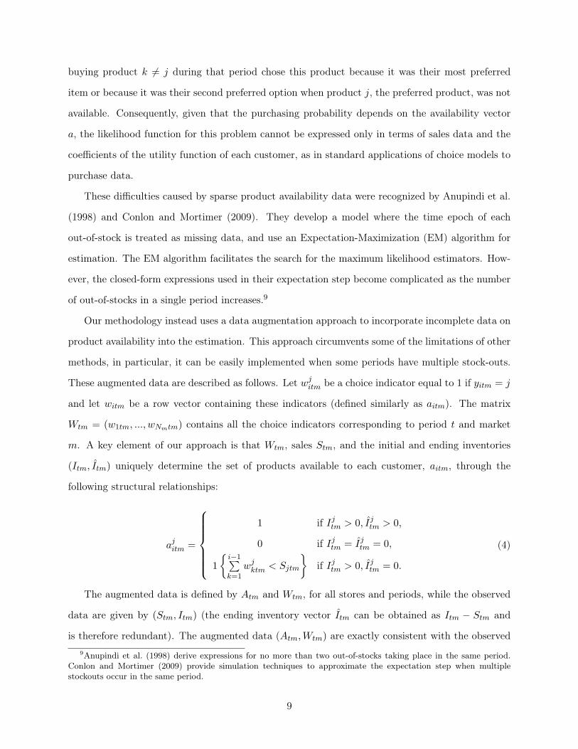
buying product k ∕= j during that period chose this product because it was their most preferred

item or because it was their second preferred option when product j, the preferred product, was not

available. Consequently, given that the purchasing probability depends on the availability vector

a, the likelihood function for this problem cannot be expressed only in terms of sales data and the

coefficients of the utility function of each customer, as in standard applications of choice models to

purchase data.

These difficulties caused by sparse product availability data were recognized by Anupindi et al.

(1998) and Conlon and Mortimer (2009). They develop a model where the time epoch of each

out-of-stock is treated as missing data, and use an Expectation-Maximization (EM) algorithm for

estimation. The EM algorithm facilitates the search for the maximum likelihood estimators. How-

ever, the closed-form expressions used in their expectation step become complicated as the number

of out-of-stocks in a single period increases.9

Our methodology instead uses a data augmentation approach to incorporate incomplete data on

product availability into the estimation. This approach circumvents some of the limitations of other

methods, in particular, it can be easily implemented when some periods have multiple stock-outs.

These augmented data are described as follows. Let wjitm be a choice indicator equal to 1 if yitm = j

and let witm be a row vector containing these indicators (defined similarly as aitm). The matrix

Wtm = (w1tm, ..., wNmtm) contains all the choice indicators corresponding to period t and market

m. A key element of our approach is that Wtm, sales Stm, and the initial and ending inventories

(Itm, Itm) uniquely determine the set of products available to each customer, aitm, through the

following structural relationships:

ajitm =

⎧

⎨

⎩

1 if Ijtm > 0, Ijtm > 0,

0 if Ijtm = Ijtm = 0,

1

{

i−1∑

k=1

wjktm < Sjtm

}

if Ijtm > 0, Ijtm = 0.

(4)

The augmented data is defined by Atm and Wtm, for all stores and periods, while the observed

data are given by (Stm, Itm) (the ending inventory vector Itm can be obtained as Itm − Stm and

is therefore redundant). The augmented data (Atm,Wtm) are exactly consistent with the observed

9Anupindi et al. (1998) derive expressions for no more than two out-of-stocks taking place in the same period.Conlon and Mortimer (2009) provide simulation techniques to approximate the expectation step when multiplestockouts occur in the same period.

9

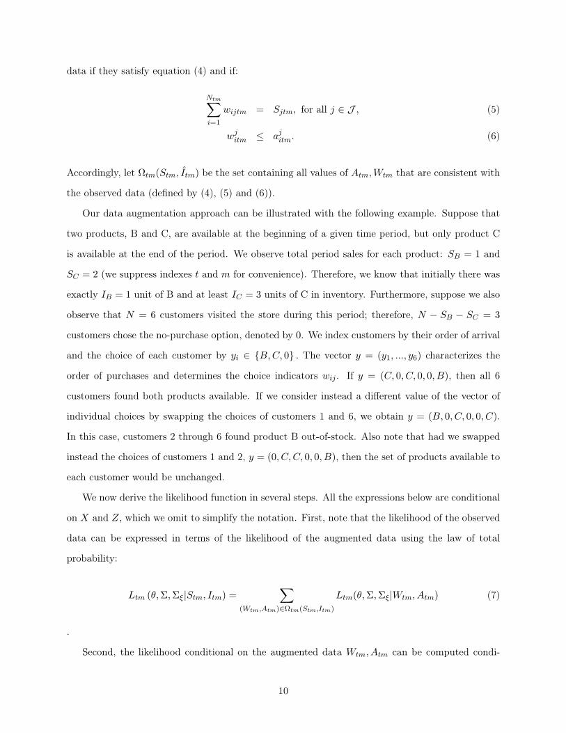
data if they satisfy equation (4) and if:

Ntm∑

i=1

wijtm = Sjtm, for all j ∈ J , (5)

wjitm ≤ ajitm. (6)

Accordingly, let Ωtm(Stm, Itm) be the set containing all values of Atm,Wtm that are consistent with

the observed data (defined by (4), (5) and (6)).

Our data augmentation approach can be illustrated with the following example. Suppose that

two products, B and C, are available at the beginning of a given time period, but only product C

is available at the end of the period. We observe total period sales for each product: SB = 1 and

SC = 2 (we suppress indexes t and m for convenience). Therefore, we know that initially there was

exactly IB = 1 unit of B and at least IC = 3 units of C in inventory. Furthermore, suppose we also

observe that N = 6 customers visited the store during this period; therefore, N − SB − SC = 3

customers chose the no-purchase option, denoted by 0. We index customers by their order of arrival

and the choice of each customer by yi ∈ {B,C, 0} . The vector y = (y1, ..., y6) characterizes the

order of purchases and determines the choice indicators wij . If y = (C, 0, C, 0, 0, B), then all 6

customers found both products available. If we consider instead a different value of the vector of

individual choices by swapping the choices of customers 1 and 6, we obtain y = (B, 0, C, 0, 0, C).

In this case, customers 2 through 6 found product B out-of-stock. Also note that had we swapped

instead the choices of customers 1 and 2, y = (0, C, C, 0, 0, B), then the set of products available to

each customer would be unchanged.

We now derive the likelihood function in several steps. All the expressions below are conditional

on X and Z, which we omit to simplify the notation. First, note that the likelihood of the observed

data can be expressed in terms of the likelihood of the augmented data using the law of total

probability:

Ltm (�,Σ,Σ�∣Stm, Itm) =∑

(Wtm,Atm)∈Ωtm(Stm,Itm)

Ltm(�,Σ,Σ�∣Wtm, Atm) (7)

.

Second, the likelihood conditional on the augmented data Wtm, Atm can be computed condi-

10

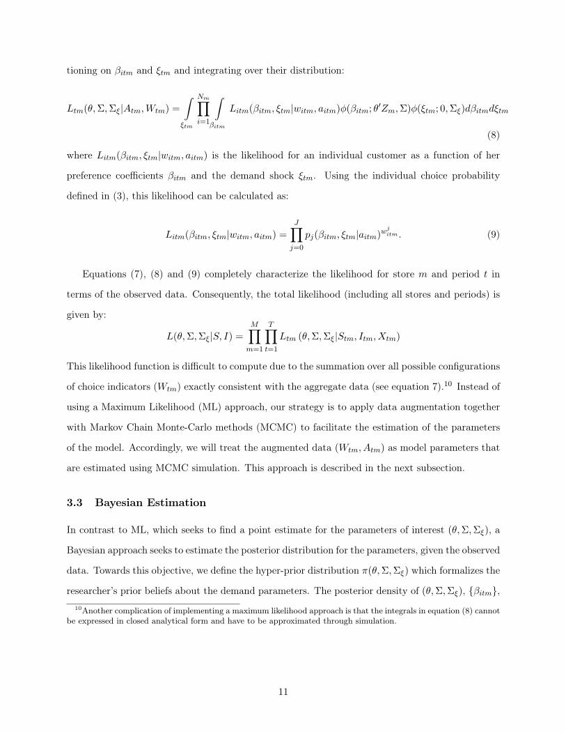
tioning on �itm and �tm and integrating over their distribution:

Ltm(�,Σ,Σ�∣Atm,Wtm) =

∫

�tm

Nm∏

i=1

∫

�itm

Litm(�itm, �tm∣witm, aitm)�(�itm; �′Zm,Σ)�(�tm; 0,Σ�)d�itmd�tm

(8)

where Litm(�itm, �tm∣witm, aitm) is the likelihood for an individual customer as a function of her

preference coefficients �itm and the demand shock �tm. Using the individual choice probability

defined in (3), this likelihood can be calculated as:

Litm(�itm, �tm∣witm, aitm) =J∏

j=0

pj(�itm, �tm∣aitm)wjitm . (9)

Equations (7), (8) and (9) completely characterize the likelihood for store m and period t in

terms of the observed data. Consequently, the total likelihood (including all stores and periods) is

given by:

L(�,Σ,Σ�∣S, I) =M∏

m=1

T∏

t=1

Ltm (�,Σ,Σ�∣Stm, Itm, Xtm)

This likelihood function is difficult to compute due to the summation over all possible configurations

of choice indicators (Wtm) exactly consistent with the aggregate data (see equation 7).10 Instead of

using a Maximum Likelihood (ML) approach, our strategy is to apply data augmentation together

with Markov Chain Monte-Carlo methods (MCMC) to facilitate the estimation of the parameters

of the model. Accordingly, we will treat the augmented data (Wtm, Atm) as model parameters that

are estimated using MCMC simulation. This approach is described in the next subsection.

3.3 Bayesian Estimation

In contrast to ML, which seeks to find a point estimate for the parameters of interest (�,Σ,Σ�), a

Bayesian approach seeks to estimate the posterior distribution for the parameters, given the observed

data. Towards this objective, we define the hyper-prior distribution �(�,Σ,Σ�) which formalizes the

researcher’s prior beliefs about the demand parameters. The posterior density of (�,Σ,Σ�), {�itm},

10Another complication of implementing a maximum likelihood approach is that the integrals in equation (8) cannotbe expressed in closed analytical form and have to be approximated through simulation.

11

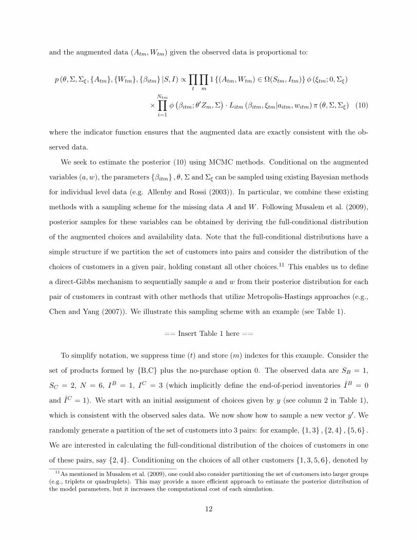
and the augmented data (Atm,Wtm) given the observed data is proportional to:

p (�,Σ,Σ�, {Atm}, {Wtm}, {�itm} ∣S, I) ∝∏

t

∏

m

1 {(Atm,Wtm) ∈ Ω(Stm, Itm)}� (�tm; 0,Σ�)

×

Ntm∏

i=1

�(

�itm; �′Zm,Σ)

⋅ Litm (�itm, �tm∣aitm, witm)� (�,Σ,Σ�) (10)

where the indicator function ensures that the augmented data are exactly consistent with the ob-

served data.

We seek to estimate the posterior (10) using MCMC methods. Conditional on the augmented

variables (a, w), the parameters {�itm} , �, Σ and Σ� can be sampled using existing Bayesian methods

for individual level data (e.g. Allenby and Rossi (2003)). In particular, we combine these existing

methods with a sampling scheme for the missing data A and W . Following Musalem et al. (2009),

posterior samples for these variables can be obtained by deriving the full-conditional distribution

of the augmented choices and availability data. Note that the full-conditional distributions have a

simple structure if we partition the set of customers into pairs and consider the distribution of the

choices of customers in a given pair, holding constant all other choices.11 This enables us to define

a direct-Gibbs mechanism to sequentially sample a and w from their posterior distribution for each

pair of customers in contrast with other methods that utilize Metropolis-Hastings approaches (e.g.,

Chen and Yang (2007)). We illustrate this sampling scheme with an example (see Table 1).

== Insert Table 1 here ==

To simplify notation, we suppress time (t) and store (m) indexes for this example. Consider the

set of products formed by {B,C} plus the no-purchase option 0. The observed data are SB = 1,

SC = 2, N = 6, IB = 1, IC = 3 (which implicitly define the end-of-period inventories IB = 0

and IC = 1). We start with an initial assignment of choices given by y (see column 2 in Table 1),

which is consistent with the observed sales data. We now show how to sample a new vector y′. We

randomly generate a partition of the set of customers into 3 pairs: for example, {1, 3} , {2, 4} , {5, 6} .

We are interested in calculating the full-conditional distribution of the choices of customers in one

of these pairs, say {2, 4}. Conditioning on the choices of all other customers {1, 3, 5, 6}, denoted by

11As mentioned in Musalem et al. (2009), one could also consider partitioning the set of customers into larger groups(e.g., triplets or quadruplets). This may provide a more efficient approach to estimate the posterior distribution ofthe model parameters, but it increases the computational cost of each simulation.

12

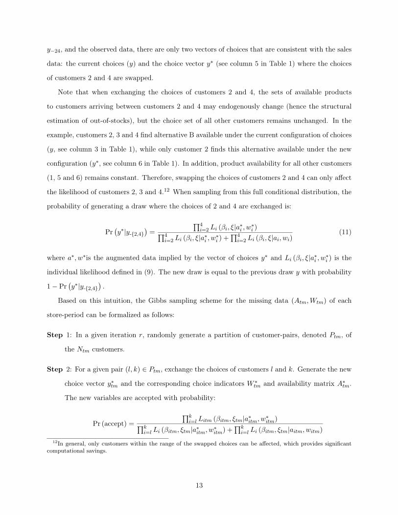
y−24, and the observed data, there are only two vectors of choices that are consistent with the sales

data: the current choices (y) and the choice vector y∗ (see column 5 in Table 1) where the choices

of customers 2 and 4 are swapped.

Note that when exchanging the choices of customers 2 and 4, the sets of available products

to customers arriving between customers 2 and 4 may endogenously change (hence the structural

estimation of out-of-stocks), but the choice set of all other customers remains unchanged. In the

example, customers 2, 3 and 4 find alternative B available under the current configuration of choices

(y, see column 3 in Table 1), while only customer 2 finds this alternative available under the new

configuration (y∗, see column 6 in Table 1). In addition, product availability for all other customers

(1, 5 and 6) remains constant. Therefore, swapping the choices of customers 2 and 4 can only affect

the likelihood of customers 2, 3 and 4.12 When sampling from this full conditional distribution, the

probability of generating a draw where the choices of 2 and 4 are exchanged is:

Pr(

y∗∣y-{2,4}

)

=

∏4i=2 Li (�i, �∣a

∗i , w

∗i )

∏4i=2 Li (�i, �∣a∗i , w

∗i ) +

∏4i=2 Li (�i, �∣ai, wi)

(11)

where a∗, w∗is the augmented data implied by the vector of choices y∗ and Li (�i, �∣a∗i , w

∗i ) is the

individual likelihood defined in (9). The new draw is equal to the previous draw y with probability

1− Pr(

y∗∣y-{2,4}

)

.

Based on this intuition, the Gibbs sampling scheme for the missing data (Atm,Wtm) of each

store-period can be formalized as follows:

Step 1: In a given iteration r, randomly generate a partition of customer-pairs, denoted Ptm, of

the Ntm customers.

Step 2: For a given pair (l, k) ∈ Ptm, exchange the choices of customers l and k. Generate the new

choice vector y∗tm and the corresponding choice indicators W ∗tm and availability matrix A∗

tm.

The new variables are accepted with probability:

Pr (accept) =

∏ki=l Litm (�itm, �tm∣a

∗itm, w∗

itm)∏k

i=l Li (�itm, �tm∣a∗itm, w∗itm) +

∏ki=l Li (�itm, �tm∣aitm, witm)

12In general, only customers within the range of the swapped choices can be affected, which provides significantcomputational savings.

13

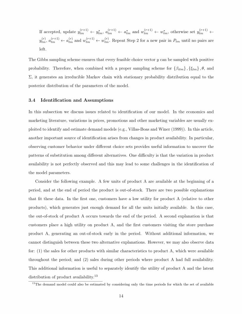
If accepted, update y(r+1)tm ← y∗tm, a

(r+1)tm ← a∗tm and w

(r+1)tm ← w∗

tm, otherwise set y(r+1)tm ←

y(r)tm , a

(r+1)tm ← a

(r)tm and w

(r+1)tm ← w

(r)tm. Repeat Step 2 for a new pair in Ptm until no pairs are

left.

The Gibbs sampling scheme ensures that every feasible choice vector y can be sampled with positive

probability. Therefore, when combined with a proper sampling scheme for {�itm} , {�tm} , �, and

Σ, it generates an irreducible Markov chain with stationary probability distribution equal to the

posterior distribution of the parameters of the model.

3.4 Identification and Assumptions

In this subsection we discuss issues related to identification of our model. In the economics and

marketing literature, variations in prices, promotions and other marketing variables are usually ex-

ploited to identify and estimate demand models (e.g., Villas-Boas and Winer (1999)). In this article,

another important source of identification arises from changes in product availability. In particular,

observing customer behavior under different choice sets provides useful information to uncover the

patterns of substitution among different alternatives. One difficulty is that the variation in product

availability is not perfectly observed and this may lead to some challenges in the identification of

the model parameters.

Consider the following example. A few units of product A are available at the beginning of a

period, and at the end of period the product is out-of-stock. There are two possible explanations

that fit these data. In the first one, customers have a low utility for product A (relative to other

products), which generates just enough demand for all the units initially available. In this case,

the out-of-stock of product A occurs towards the end of the period. A second explanation is that

customers place a high utility on product A, and the first customers visiting the store purchase

product A, generating an out-of-stock early in the period. Without additional information, we

cannot distinguish between these two alternative explanations. However, we may also observe data

for: (1) the sales for other products with similar characteristics to product A, which were available

throughout the period; and (2) sales during other periods where product A had full availability.

This additional information is useful to separately identify the utility of product A and the latent

distribution of product availability.13

13The demand model could also be estimated by considering only the time periods for which the set of available

14

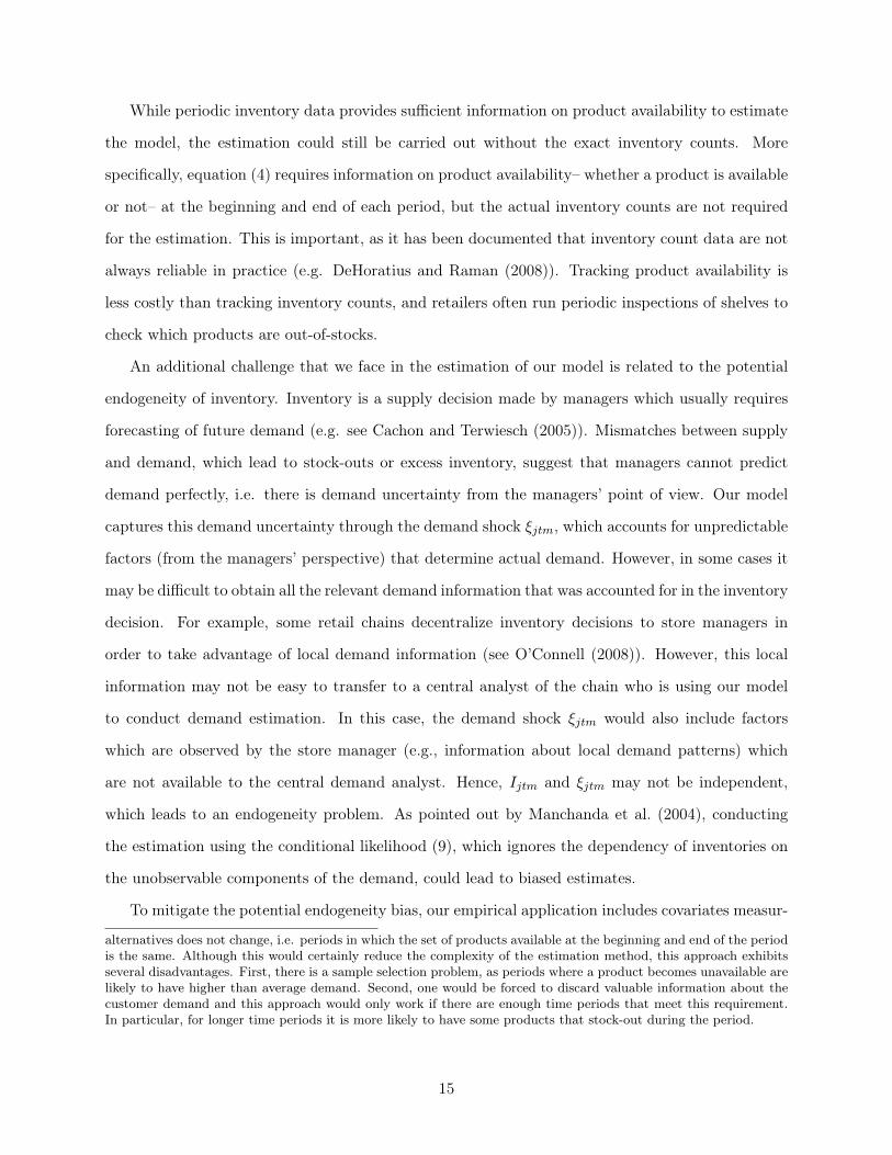
While periodic inventory data provides sufficient information on product availability to estimate

the model, the estimation could still be carried out without the exact inventory counts. More

specifically, equation (4) requires information on product availability– whether a product is available

or not– at the beginning and end of each period, but the actual inventory counts are not required

for the estimation. This is important, as it has been documented that inventory count data are not

always reliable in practice (e.g. DeHoratius and Raman (2008)). Tracking product availability is

less costly than tracking inventory counts, and retailers often run periodic inspections of shelves to

check which products are out-of-stocks.

An additional challenge that we face in the estimation of our model is related to the potential

endogeneity of inventory. Inventory is a supply decision made by managers which usually requires

forecasting of future demand (e.g. see Cachon and Terwiesch (2005)). Mismatches between supply

and demand, which lead to stock-outs or excess inventory, suggest that managers cannot predict

demand perfectly, i.e. there is demand uncertainty from the managers’ point of view. Our model

captures this demand uncertainty through the demand shock �jtm, which accounts for unpredictable

factors (from the managers’ perspective) that determine actual demand. However, in some cases it

may be difficult to obtain all the relevant demand information that was accounted for in the inventory

decision. For example, some retail chains decentralize inventory decisions to store managers in

order to take advantage of local demand information (see O’Connell (2008)). However, this local

information may not be easy to transfer to a central analyst of the chain who is using our model

to conduct demand estimation. In this case, the demand shock �jtm would also include factors

which are observed by the store manager (e.g., information about local demand patterns) which

are not available to the central demand analyst. Hence, Ijtm and �jtm may not be independent,

which leads to an endogeneity problem. As pointed out by Manchanda et al. (2004), conducting

the estimation using the conditional likelihood (9), which ignores the dependency of inventories on

the unobservable components of the demand, could lead to biased estimates.

To mitigate the potential endogeneity bias, our empirical application includes covariates measur-

alternatives does not change, i.e. periods in which the set of products available at the beginning and end of the periodis the same. Although this would certainly reduce the complexity of the estimation method, this approach exhibitsseveral disadvantages. First, there is a sample selection problem, as periods where a product becomes unavailable arelikely to have higher than average demand. Second, one would be forced to discard valuable information about thecustomer demand and this approach would only work if there are enough time periods that meet this requirement.In particular, for longer time periods it is more likely to have some products that stock-out during the period.

15

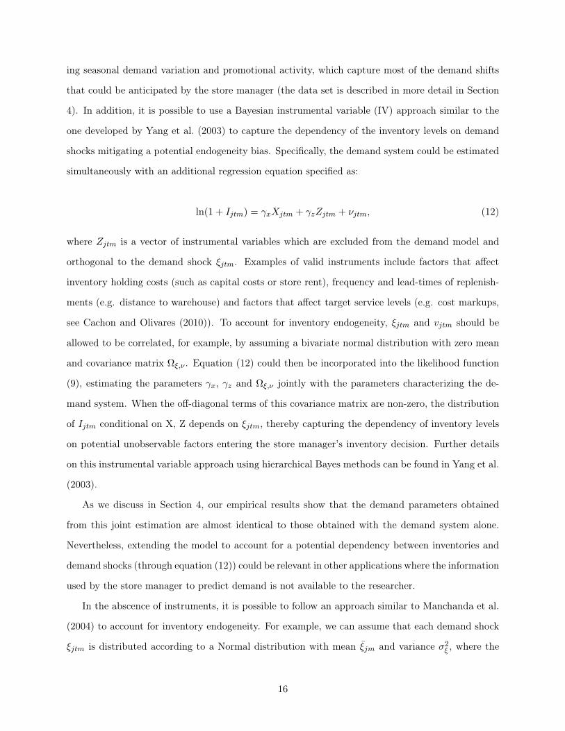
ing seasonal demand variation and promotional activity, which capture most of the demand shifts

that could be anticipated by the store manager (the data set is described in more detail in Section

4). In addition, it is possible to use a Bayesian instrumental variable (IV) approach similar to the

one developed by Yang et al. (2003) to capture the dependency of the inventory levels on demand

shocks mitigating a potential endogeneity bias. Specifically, the demand system could be estimated

simultaneously with an additional regression equation specified as:

ln(1 + Ijtm) = xXjtm + zZjtm + �jtm, (12)

where Zjtm is a vector of instrumental variables which are excluded from the demand model and

orthogonal to the demand shock �jtm. Examples of valid instruments include factors that affect

inventory holding costs (such as capital costs or store rent), frequency and lead-times of replenish-

ments (e.g. distance to warehouse) and factors that affect target service levels (e.g. cost markups,

see Cachon and Olivares (2010)). To account for inventory endogeneity, �jtm and vjtm should be

allowed to be correlated, for example, by assuming a bivariate normal distribution with zero mean

and covariance matrix Ω�,� . Equation (12) could then be incorporated into the likelihood function

(9), estimating the parameters x, z and Ω�,� jointly with the parameters characterizing the de-

mand system. When the off-diagonal terms of this covariance matrix are non-zero, the distribution

of Ijtm conditional on X, Z depends on �jtm, thereby capturing the dependency of inventory levels

on potential unobservable factors entering the store manager’s inventory decision. Further details

on this instrumental variable approach using hierarchical Bayes methods can be found in Yang et al.

(2003).

As we discuss in Section 4, our empirical results show that the demand parameters obtained

from this joint estimation are almost identical to those obtained with the demand system alone.

Nevertheless, extending the model to account for a potential dependency between inventories and

demand shocks (through equation (12)) could be relevant in other applications where the information

used by the store manager to predict demand is not available to the researcher.

In the abscence of instruments, it is possible to follow an approach similar to Manchanda et al.

(2004) to account for inventory endogeneity. For example, we can assume that each demand shock

�jtm is distributed according to a Normal distribution with mean �jm and variance �2� , where the

16

means are treated as random coefficients. If we replace Zjtm by �jm in equation (12) and assume that

Cov(�jtm, �jtm− �jm) = 0, our model becomes a special case of the model developed by Manchanda

et al. (2004), which can be estimated with the Bayesian techniques described therein.

Finally, another potential endogeneity problem may arise from serially correlated demand shocks

(�jtm). Today’s inventory depends on yesterday’s demand, which induces a correlation between

current inventory and previous demand shocks. In addition, if demand shocks are autocorrelated,

current demand shocks will be correlated with previous shocks that are in turn correlated with

today’s initial inventory, leading to an endogeneity problem. As we previously mentioned, we do

not expect to observe autocorrelation in demand shocks in our application once we control for

seasonality. Nevertheless, the methodology presented here could be extended to allow for demand

shock persistence, which would eliminate this form of endogeneity.

3.5 Numerical Experiment

In this subsection, we test the proposed methodology using simulated data. We generated sales

and inventory data for J = 10 purchase alternatives and a no-purchase option available in M = 12

markets and T = 15 periods. We included four variables (x1, ..., x4) in the utility function. We

use random coefficients for x3 and x4 and assume fixed (i.e., constant across customers in a given

market) coefficients for x1 and x2. The first two variables correspond to two brands dummies, one

for alternatives 1, 2 and 3 (x1), and another for alternatives 4, 5 and 6 (x2). The third variable is a

dummy variable equal to 1 for all purchase alternatives (x3), while the fourth variable is generated

from a normal distribution (x4). In order to replicate some of the features of the data set used in

our empirical application, the continuous variable is generated so that its values for a given brand

and market are the same across all time periods. Accordingly, the values of x4 for each brand and

market are generated from a normal distribution with mean equal to 2 and variance equal to 1.

Based on these four explanatory variables, customer coefficients for a given market m are gen-

erated from a 4-dimensional multivariate normal distribution with mean �m = �′Zm as in equation

(2) and variance Σ, where Zm represents a 2-dimensional vector of demographic variables. In terms

of the demographics, the first variable z1m is equal to 1 for all markets (intercept), while the second

variable z2m is generated from a uniform distribution in the interval [−1.5, 1.5]. The true value of

17

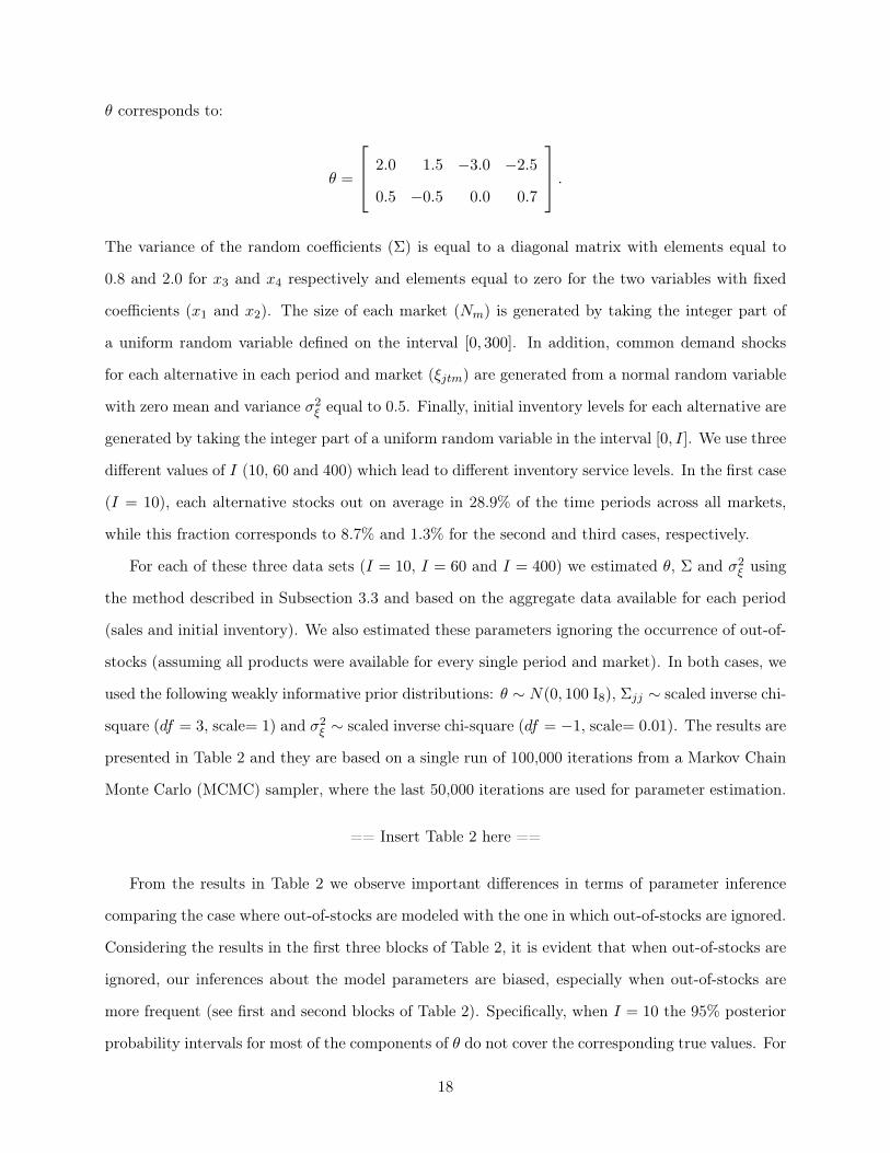
� corresponds to:

� =

⎡

⎢

⎣

2.0 1.5 −3.0 −2.5

0.5 −0.5 0.0 0.7

⎤

⎥

⎦.

The variance of the random coefficients (Σ) is equal to a diagonal matrix with elements equal to

0.8 and 2.0 for x3 and x4 respectively and elements equal to zero for the two variables with fixed

coefficients (x1 and x2). The size of each market (Nm) is generated by taking the integer part of

a uniform random variable defined on the interval [0, 300]. In addition, common demand shocks

for each alternative in each period and market (�jtm) are generated from a normal random variable

with zero mean and variance �2� equal to 0.5. Finally, initial inventory levels for each alternative are

generated by taking the integer part of a uniform random variable in the interval [0, I]. We use three

different values of I (10, 60 and 400) which lead to different inventory service levels. In the first case

(I = 10), each alternative stocks out on average in 28.9% of the time periods across all markets,

while this fraction corresponds to 8.7% and 1.3% for the second and third cases, respectively.

For each of these three data sets (I = 10, I = 60 and I = 400) we estimated �, Σ and �2� using

the method described in Subsection 3.3 and based on the aggregate data available for each period

(sales and initial inventory). We also estimated these parameters ignoring the occurrence of out-of-

stocks (assuming all products were available for every single period and market). In both cases, we

used the following weakly informative prior distributions: � ∼ N(0, 100 I8), Σjj ∼ scaled inverse chi-

square (df = 3, scale= 1) and �2� ∼ scaled inverse chi-square (df = −1, scale= 0.01). The results are

presented in Table 2 and they are based on a single run of 100,000 iterations from a Markov Chain

Monte Carlo (MCMC) sampler, where the last 50,000 iterations are used for parameter estimation.

== Insert Table 2 here ==

From the results in Table 2 we observe important differences in terms of parameter inference

comparing the case where out-of-stocks are modeled with the one in which out-of-stocks are ignored.

Considering the results in the first three blocks of Table 2, it is evident that when out-of-stocks are

ignored, our inferences about the model parameters are biased, especially when out-of-stocks are

more frequent (see first and second blocks of Table 2). Specifically, when I = 10 the 95% posterior

probability intervals for most of the components of � do not cover the corresponding true values. For

18

example, �z1,x3 which is used to derive the mean utility of all the purchase options is underestimated

when out-of-stocks are ignored (true value= −3, 95% posterior probability interval: [−4.60,−3.78]).

In addition, the heterogeneity in the random coefficients for the continuous variable (Σx4,x4 , true

value= 2, 95% posterior probability interval: [0.54, 1.46]) is underestimated. As expected, the

estimation results for the naïve model improve as out-of-stocks become less frequent. In particular,

in the third case, where out-of-stocks are on-average observed only in 1.3% of the time periods for

each alternative(I = 400), the results are very similar across both models (see third and sixth blocks

in Table 2), a good sign for our approach.

In terms of the full model, the results in the last three blocks in Table 2 show that the method

recovers well the original parameters under each of the three scenarios. In fact, the posterior

means are close to their true values (on average within 0.8 posterior standard deviations from the

corresponding true values). In addition, in all but four cases (�z1,x3 and Σx3,x3 in the fifth block and

�z1,x2 and Σ� in the sixth block of Table 2), the true values are contained within the 95% posterior

probability intervals.

Finally, it is important to mention that we also conducted an additional simulation study by

generating 50 data sets for the case where I = 10. We estimated the model parameters using the

proposed method and also ignoring the occurrence of out-of-stocks. The results of this simulation

study, confirm the basic findings discussed in this subsection (please refer to Online Appendix A).

3.6 Estimating Lost Sales

An important factor that determines inventory levels in retailing is the cost of shortage. This

cost is closely related to the behavior of customers that encounter an out-of-stock. The cost of an

out-of-stock increases with: (i) the markup of the product that sells out; and (ii) the fraction of

customers that choose not to purchase after experiencing an out-of-stock.14 The former is known

by the store manager, but the latter is not directly observable. In what follows, we show how to use

the model to estimate lost sales - the fraction of customers that chose not to purchase but would

have purchased if some of the out-of-stock products had been available- for a given inventory policy.

This estimate can be used to compute performance measures such as the fill-rate, defined as the

14Also note that the cost of an out-of-stock decreases with the markup of the products that capture the demandfor the non-available products and leads to the possibility of “strategic out-of-stocks” by the retailer, which we do notpursue here.

19

fraction of demand filled from stock, which is commonly used in retail operations management. It

can also be used together with markup information to assign a dollar value to the cost of shortage.

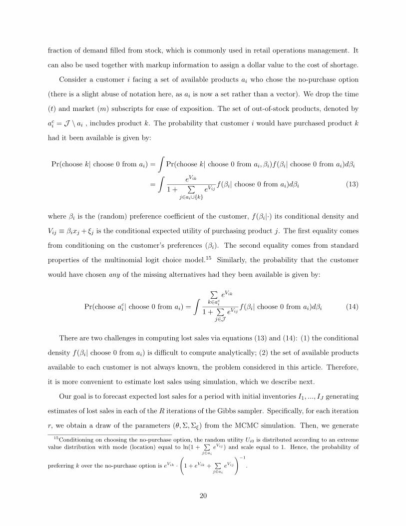
Consider a customer i facing a set of available products ai who chose the no-purchase option

(there is a slight abuse of notation here, as ai is now a set rather than a vector). We drop the time

(t) and market (m) subscripts for ease of exposition. The set of out-of-stock products, denoted by

aci = J ∖ ai , includes product k. The probability that customer i would have purchased product k

had it been available is given by:

Pr(choose k∣ choose 0 from ai) =

∫

Pr(choose k∣ choose 0 from ai, �i)f(�i∣ choose 0 from ai)d�i

=

∫

eVik

1 +∑

j∈ai∪{k}

eVijf(�i∣ choose 0 from ai)d�i (13)

where �i is the (random) preference coefficient of the customer, f(�i∣⋅) its conditional density and

Vij ≡ �ixj + �j is the conditional expected utility of purchasing product j. The first equality comes

from conditioning on the customer’s preferences (�i). The second equality comes from standard

properties of the multinomial logit choice model.15 Similarly, the probability that the customer

would have chosen any of the missing alternatives had they been available is given by:

Pr(choose aci ∣ choose 0 from ai) =

∫

∑

k∈aci

eVik

1 +∑

j∈J

eVijf(�i∣ choose 0 from ai)d�i (14)

There are two challenges in computing lost sales via equations (13) and (14): (1) the conditional

density f(�i∣ choose 0 from ai) is difficult to compute analytically; (2) the set of available products

available to each customer is not always known, the problem considered in this article. Therefore,

it is more convenient to estimate lost sales using simulation, which we describe next.

Our goal is to forecast expected lost sales for a period with initial inventories I1, ..., IJ generating

estimates of lost sales in each of the R iterations of the Gibbs sampler. Specifically, for each iteration

r, we obtain a draw of the parameters (�,Σ,Σ�) from the MCMC simulation. Then, we generate

15Conditioning on choosing the no-purchase option, the random utility Ui0 is distributed according to an extremevalue distribution with mode (location) equal to ln(1 +

∑

j∈ai

eVij ) and scale equal to 1. Hence, the probability of

preferring k over the no-purchase option is eVik⋅

(

1 + eVik +∑

j∈ai

eVij

)

−1

.

20

N new draws of �i from a MVN(�′Z,Σ) (one for each customer) and � from a MVN(0,Σ�). These

can be used to calculate the expected utilities Vij = �ixj + �j for each customer and product.

Next, we sequentially simulate the choices of each customer. Specifically, given the initial inven-

tories, we determine the set of products available to the first customer, a1, and sample the customer

choice, y1, from a multinomial distribution with probabilities specified by (3). Given this choice, we

update inventories by subtracting one unit from the chosen product (unless y1 = 0, in which case

inventories remain unchanged) and proceed to next customer. The process is repeated for all the

N customers. Customers who chose the no-purchase alternative are recorded in the set Or (keeping

the corresponding values of the Vij ’s and ai). Accordingly, the expected lost sales can be estimated

as follows:

E(LostSales) =1

∣R∣

R∑

r=1

∑

i∈Or

∑

k∈aci

eV(r)ik

1 +∑

j∈J

eV(r)ij

. (15)

where V(r)ij denotes the value of Vij in iteration r. This simulation procedure can be used to forecast

lost sales for any initial inventory levels I1, ..., IJ . Alternatively, one could estimate lost sales

retrospectively for a time period where the observed data on inventories and sales were collected.

The only adjustment to this method is that samples of �i, ai, �iand yi are directly obtained from the

MCMC simulation used in the estimation. This ensures that the distribution of customer preferences

and availability are conditioned on the observed data.

We tested the accuracy of this method to estimate expected lost sales using the simulated

data described in Subsection 3.5. Actual lost sales were calculated using the simulated utilities by

counting customers who chose the outside good, but would have purchased a product under a full

assortment. We compared these actual lost sales with those estimated using equation (15) and the

estimated parameters. The correlation between the actual and estimated lost sales is 98.2% and the

mean absolute percentage error (MAPE) is 11.99%. Overall, this method provides a fairly accurate

estimate of the expected lost sales for a wide range of inventory levels.

A similar simulation approach can be used to estimate stockout-based substitution. At the end

of each iteration r, we can store the set of customers Pr that purchased any available product. The

number of these customers that would have instead purchased the out-of-stock product k when all

21

products are available can be estimated as:

E(Substitution[k]) =1

∣R∣

R∑

r=1

∑

i∈Pr

eV(r)ik

1 +∑

j∈J

eV(r)ij

. (16)

The next section describes an application of the methodology based on data from the shampoo

product category.

4 Empirical Application: Demand Estimation in the Shampoo Prod-

uct Category

We use data on shampoo purchases from six supermarket stores located in different regions of Spain

to illustrate the methodology. The stores are owned by a major supermarket chain, with more than

400 stores in this country. The data set was collected from 6 of these stores including daily sales

during 15 consecutive days (excluding two Sundays in which stores are closed) between May 13th

and May 29th in 1999. The product category includes 24 different stock keeping units (SKUs),

but not all SKUs were offered in each store during the study period. In addition to the sales data,

information about product availability on the shelf was recorded at the beginning and end of each

day. In total, 291 days with zero final inventory were recorded across all days, stores and products.

The data also contain price and promotion information for every product on each store-day.

From the 24 products in the data set, 16 products exhibited price variation across stores, but very

few products exhibited temporal price variation within a given store during the study period. Table

3 displays the brands of each product and shows summary statistics for each of the products in

terms of daily unit sales, prices (in Spanish Pesetas), promotion incidence, availability (OOS) and

number of stores where each product is offered (Stores).16

== Insert Table 3 here ==

4.1 Model specification

We include nine covariates (Xjtm) in the utility function of each customer. Two of these covariates

have random coefficients: price and purchase option. The latter is a dummy variable equal to 1 in

16Availability is measured as the fraction of days with zero end inventory for a given product.

22

every period for all options except the no-purchase option. This variable captures total category

demand for shampoo products as higher coefficients associated to this variable raise the utility of

all purchase alternatives in relation to the utility of the no-purchase option. In addition, we include

dummy variables for the following brands: Pantene, Herbal Essence, Head & Shoulders (H&S),

Cabello Sano and Timotei. We also include a dummy variables (Weekend) to control for seasonality

(changes in demand during weekends). This variable is equal to 1 for all purchase alternatives for

every time period corresponding to a Saturday and is equal to 0 otherwise (recall that the stores

are closed on Sundays). Finally, we control for promotional effects by using a dummy variable

(Promotion) equal to 1 if an item was promoted and zero otherwise during a given time period and

store. We note that these last two variables (Weekend and Promotion) also enable us to explicitly

consider in the utility function changes in demand that might be anticipated by the store manager,

given that promotional activity can (and is expected) to cause increased demand.

We use store-level demographic information to capture observed preference heterogeneity across

stores (unobserved heterogeneity is captured through random coefficients). Specifically, we collected

information on average declared income for each market. Accordingly, the vector of demographic

variables for a given store m (Zm) has two components: an indicator equal to 1 for all stores

(intercept) and the standardized natural logarithm of income17. In addition, the size of the market

for each store was estimated combining data on population and total consumption of shampoo in

Spain18. We note that, as it is common in the marketing and economics literature, the market size

is assumed to be constant across time periods, although it is important to highlight that our model

allows for a different fraction of the market to make purchases in different periods19.

17We also experimented using additional demographic information (e.g., age), but the results and the fit of themodel do not substantially change.

18The population data were downloaded from http://www.ine.es, while the consumption data were obtained fromEuromonitor International. We also experimented with an alternative definition of the market size (approximatelytwice the size of the one used in this section) and obtained very similar results.

19We also tested the consequences of this assumption using simulated data where the market size fluctuates overtime and estimating this model assuming the market size is constant and equal to its average. When the variability ofthe market size increases, we find a slight decrease in the estimated variance of the intercepts that affect the utility ofall purchase alternatives and a slight increase in the estimated variance of the demand shocks. The mean of consumercoefficients does not exhibit any systematic changes. Detailed results are available from the authors upon request.

23

4.2 Results

Using the method introduced in Section 3, we estimated the model based on the covariates and

demographic variables previously described. We also estimated a benchmark model that ignores

out-of-stocks, i.e. every product offered in a given store is assumed to be available to all customers in

every time period. However, products that were never available in a particular store were excluded

from the choice set in the benchmark model. We computed the log-marginal likelihood for the

full and benchmark models and obtained a log-Bayes Factor equal to 74.5, which gives very strong

empirical support for the full model (Kass and Raftery (1995)). Table 4 reports the estimation

results for the hyper-parameters �, Σ and �2� under both model specifications.

== Insert Table 4 here ==

From the results of the full model we note that products from the brands Herbal Essence

and H&S are on average more demanded than all other products (see the results for �Intercept

in Table 4). Furthermore, the results for �Income show higher intrinsic demand for Pantene and

H&S products in stores reaching customers with higher income levels. As expected, the price,

weekend and promotion effects (see �Intercept,Price, �Intercept,Weekend and �Intercept,Promotion) show

a significant disutility associated with higher prices and higher levels of demand during Saturdays

and when items are promoted. These results also show that the promotional and weekend effects

are stronger for lower-income markets.

In addition to the observed heterogeneity across stores captured by �Income, the results for Σ show

the magnitude of the unobserved heterogeneity within stores in terms of total demand (Purchase

option) and price sensitivity (Price). The variances for these random coefficients are estimated as

0.70 and 0.24, respectively. The results for the variance of the demand shocks (�2� ) suggest that

these unobserved demand effects are substantial (the posterior mean of �2� is estimated as 1.00).

Finally, when comparing the full and benchmark models, we note that the posterior means of

�Intercept for the brands Pantene, H&S and Cabello Sano are smaller under the benchmark model

than in the full model (these posterior means are approximately one posterior standard deviation

from each other). These differences do not exhibit a strong level of statistical significance, but

their direction suggests that ignoring out-of-stocks leads to lower estimates of demand for these

brands. In contrast, the corresponding posterior mean for Herbal Essence is very similar across

24

both models, which is consistent with the high availability of this product on the shelf (92%, see

fraction of out-of-stocks for product 17 in Table 3).

We tested the robustness of these results with respect to a potential inventory endogeneity bias.

Using the extensions described in Subsection 3.4, we accounted for a possible correlation between

inventory and the demand shocks by adding equation (12) into the estimation, which helps to

mitigate this endogeneity problem. We used the products’ cost markup as an instrumental variable,

which varies across products and stores but not across days. The results from this extended model

suggest a small correlation between inventory and demand shocks (the estimated posterior mean

of the correlation between � and � is equal to 0.26)20. Furthermore, there is strong empirical

support favoring the model where the correlation between � and � is zero (log-Bayes Factor=

−716.6). The estimated marginal posterior distribution of each parameter in the extended model

exhibits a reasonable precision, suggesting that the parameters are identified after controlling for

inventory endogeneity (see Allenby and Rossi (2003) for more details on identification of Bayesian

IV models). In addition, the estimated demand parameters from this extended model and the full

model presented in Subsection 4.2 are very similar (results are available from the authors upon

request), which implies that the potential bias due to inventory endogeneity is small. Recall that

the demand specification of this application includes factors that measure seasonality, promotional

activity and brand effects, capturing most of the variation in demand that can be anticipated by

the store manager. This helps to reduce endogeneity problems arising from omitted variables in the

demand specification.

5 Estimating and Mitigating the Costs of Out-Of-Stocks

Using the expressions derived in Subsection 3.6 (see equation 15), we estimated lost sales for every

time period in each store. We are particularly interested in estimating how the number of out-of-

stock products affects lost sales. In our application, the number of products simultaneously out-

of-stock on a given day ranges between 0 and 10 SKUs. Our methodology is sufficiently flexible to

estimate lost sales for all of these possible scenarios without increasing the computational complexity

20Interestingly, we obtained a positive coefficient for price margin, which is consistent with theoretical predictionsfrom the inventory management literature (e.g. Porteus (2002)). Detailed results about this sensitivity analysis areavailable from the authors upon request.

25

of the method. Figure 1 shows the estimated average lost sales as a function of the number of out-

of-stock products. The figure reveals that lost sales increases non-linearly in the number of products

not available. When five or fewer products are out-of-stock the average lost sales are equal to 5.9%

of the full availability sales. But when six or more products are out-of-stock, lost sales grow by

more than 3 times, up to 20.2% of the full-availability sales. This suggests that the first products

that stock-out have a smaller impact on category sales, but lost sales increase more rapidly as more

products become unavailable. This pattern has important implications for assortment planning and

inventory replenishment decisions. In supermarkets, there are substantial fixed costs of replenishing

products on the shelf. Hence, Figure 1 suggests that replenishments may be postponable until

several products become out-of-stock without substantially affecting category sales, although the

profitability consequences of such a policy will depend on the retail margins of each of the products

and the stockout-based substitution patterns.

== Insert Figure 1 here ==

Note that in this analysis lost sales are estimated for each period and store in our data set.

Alternatively, one could estimate lost sales for a new time period by simulating a sequence of

consumers making choice decisions under limited and infinite inventory levels. In the context of the

MCMC estimation, this analysis can be easily performed and we use these results for a particular

store (store 5) to illustrate how consumers switch from one product to another when their most

preferred item is not available. As we show in Table 5, for the segment of customers who intend

to buy each product i (row) we estimate the percentage that choose instead alternative j (column)

considering representative levels of product inventory and the utility function covariates. The NP

column shows the customer that choose not to purchase, which are counted as lost sales. This

analysis enables us to provide a detailed characterization of the expected consequences of out-of-

stocks on customers’ buying behavior21.

== Insert Table 5 here ==

Specifically, the diagonal elements in the first block of this matrix indicate the percentage of

customers that are able to find their most preferred product and, consequently, provide an estimate

21For space considerations, we display the results of this analysis for only 10 of the 24 products for store 5. Therefore,the sum of the substitution rates in each of the rows of Table 5 is not equal to 1.

26

of the level of “service” provided by the retailer to its customers. Considering all alternatives (not

just those reported in Table 5), while some products exhibit very high levels of availability (e.g.,

products 5, 6, 17 and 22), most of them show availability levels below 50% (e.g., product 10). In

this regard, it is informative to consider the off-diagonal elements of this switching matrix. For

example, when product 10 (Pantene) is not available, most customers intending to buy that item

would not buy any of the available products: 37.3% of the customers intending to buy product

10 choose the no-purchase option compared to only 13.7% (i.e., 100%-49.0%-37.3%) that substitute

this product by an available one. Among the latter group of customers, most of these stockout-based

substitutions correspond to purchases of product 17 (Herbal Essence). Overall, we estimate that

for most products, between one and two thirds of the customers that intend to buy a product are

not able to find their most preferred alternative and decide not to buy. Finally, the last column

of Table 5 shows the change in contribution margin due lost sales and stockout-based substitution.

For most products with low availability (20% or below), contribution margins decrease between

30% and 65%. Overall, this analysis suggests that the financial consequences of out-of-stocks can

be sizable.

In addition to estimating stockout-based substitution and lost sales, we also evaluate the effect of

a strategy that seeks to mitigate the effect of out-of-stocks: conducting a temporary price reduction

for a single product to recapture a fraction of lost sales. Price discounts increase the attractiveness of

substitute products, inducing some customers whose preferred product is not available to substitute

their intended purchase with another product rather than choosing the no-purchase option. In what

follows, we show how to use our model to quantify the expected fraction of lost sales that would

be recaptured (from the no-purchase option) through this temporary price promotions. Consider

the set OA of customers who chose not to purchase when assortment A was available. Suppose

that the price of product k ∈ A is discounted by some fraction of the original price. For each

customer i ∈ OA, we define two events: (1) Ei1 is the event that customer i would have purchased

some of the unavailable products (i.e. products in Ac) had they been available; (2) Ei2 is the event

that the customer would purchase the discounted product k when only products in A are available.

All customers in OA experiencing Ei1 are counted as lost sales; those who in addition experience

Ei2 count as recaptured lost sales. Therefore, the fraction of lost sales that is recaptured can be

27

calculated as:

Lost Sales Reduction =

∑

i∈OA

Pr(Ei1, Ei2∣i ∈ OA)

LostSales,

where LostSales can be estimated using the simulation procedure described in Subsection 3.6. De-

tails on how to calculate the numerator of the expression above are shown in Online Appendix

B.

Accordingly, the model was used to measure the effectiveness of implementing price reductions

of 20% for different store-days. We consider scenarios where only one product is discounted at a

time. As an illustration, we report results for two store-days with very different levels of availability:

(i) day 3 in market 5, where 10 SKUs have zero final inventory; and (ii) day 15 in market 2, where

only one product has zero final inventory – SKU 15 (Pantene). In the case of day 3 in market 5,

a price promotion on product 17 (Herbal Essence) reduces lost sales by 2.0%; all other promotions

reduce lost sales by less than 1%. However, in the case of day 15 in market 2, it is more effective

to discount product 13 (Pantene), which leads to a lost-sales reduction of 4.2%. In this case, a

promotion of product 17 leads to a 1.6% reduction in lost sales.

The comparison of the results from these two store-days provides insights on the effectiveness of

price promotions at mitigating the consequences of out-of-stocks. In the case of day 15 in market 2

where only one product was out-of-stock, a price promotion on a product with similar characteristics

to the missing product is more effective to recapture lost sales. In contrast, when many products

are missing, it is more effective to use a price promotion on a popular product (SKU 17).

These results show that price promotions can be useful to reduce lost sales and improve customer

service. However, promotions may also have negative consequences, including: (1) a reduction in

the margin of the discounted product; (2) cannibalization of sales from other products with higher

margins.22 These consequences can also be easily estimated with our model if data on the cost

of goods sold by SKU is available. Using gross margin data from the supermarket chain under

study, we evaluated the net change in category profits accounting for the effect of increased sales,

reduced markups and cannibalization. In the case of day 3 in market 5, the promotion on product 17

increased total profits by 13.2%. In contrast, in the case of day 15 in market 2, the price promotion

22Other negative effects not considered here include stockpiling effects that occur when customers buy the promotedproduct earlier because of the discount, which leads to a cannibalization of future sales.

28

on products 13 and 17 reduces profits by 32.5% and 10.7%, respectively.23

In summary, this section illustrates how the methodology can be used to assess the consequences

of policies aimed at mitigating the costs of out-of-stocks (e.g., lost sales reduction, impact on cate-

gory profits). Many additional policy experiments could be also performed, including discounts on

multiple products and experimenting with different magnitudes for price discounts. These additional

policy experiments can be easily implemented using the estimated model. Note, however, that our

estimation and subsequent analysis do not consider any long run effects on customer behavior. For

example, some of the customers that don’t find their most preferred item available might return to

the store in future periods to buy the missing product. Alternatively, it is possible that some of

these customers might reduce their likelihood of returning to the store in future periods transferring

not only their shampoo purchases, but also those in other product categories, to competing retail-

ers. Studying these long-term effects constitutes a very interesting avenue for future research that

would probably require getting access to customer panel data with a longer time series of sales and

inventory data from multiple product categories.

6 Conclusions

In this article, we have proposed a method to capture the effects of out-of-stocks on customer

behavior using data commonly available to a store manager. Lack of precise availability data in

real-time, which is common in practical retail settings, introduces a major challenge in identifying

the effect of out-of-stocks on sales. To overcome these difficulties, our methodology simulates the

transition of the inventory on the shelf conditioning on snapshots of information about product

inventory, which can be obtained through a periodic inventory review system. These data are

combined with daily sales and pricing data to estimate a structural model of demand for a product

category.

The method has several attractive features. First, the model can be estimated using data from

multiple stores and markets. Second, our method is applicable in categories with many products

and with slow moving products exhibiting frequent out-of-stocks. Previous methods in this area

were limited by the number of products, the type of substitutions and the number of products that

23Promotions on other products, such as SKU 10, reduced lost sales by about 1% without substantially changingprofits.

29

could be simultaneously out-of-stock. Third, our structural demand model allows the evaluation

of policies to mitigate the consequences of out-of-stocks (such as temporary price promotions).

Fourth, the methodology explicitly models the distribution of the timing of out-of-stocks (which are

unobservable in periodic inventory systems), providing useful information on product availability.

In terms of future research, several interesting generalizations can be identified. Considering the

demand model, alternative specifications or behavioral assumptions could be studied (e.g., probit

model, complexity of choice decisions). In addition, the model could be extended to explicitly

consider the possibility of some customers returning to the store in future periods if they did

not find a product in a given time period. Since our methodology is based on estimating the joint

distribution of availability and sales, another possible extension could be developed for the detection

of out-of-stocks based on point-of-sales data. Finally, the model could be generalized to consider

purchase quantity decisions (e.g., Kim et al. (2002)).

In summary, we hope that the methodology presented in this article may provide useful tools

for researchers and managers to estimate the consequences of out-of-stocks and assess the impact

of policies to mitigate their costs. This issue is certainly relevant for audiences in the operations

management, marketing and economics disciplines, and we hope this work stimulates more cross-

disciplinary research in this area.

30

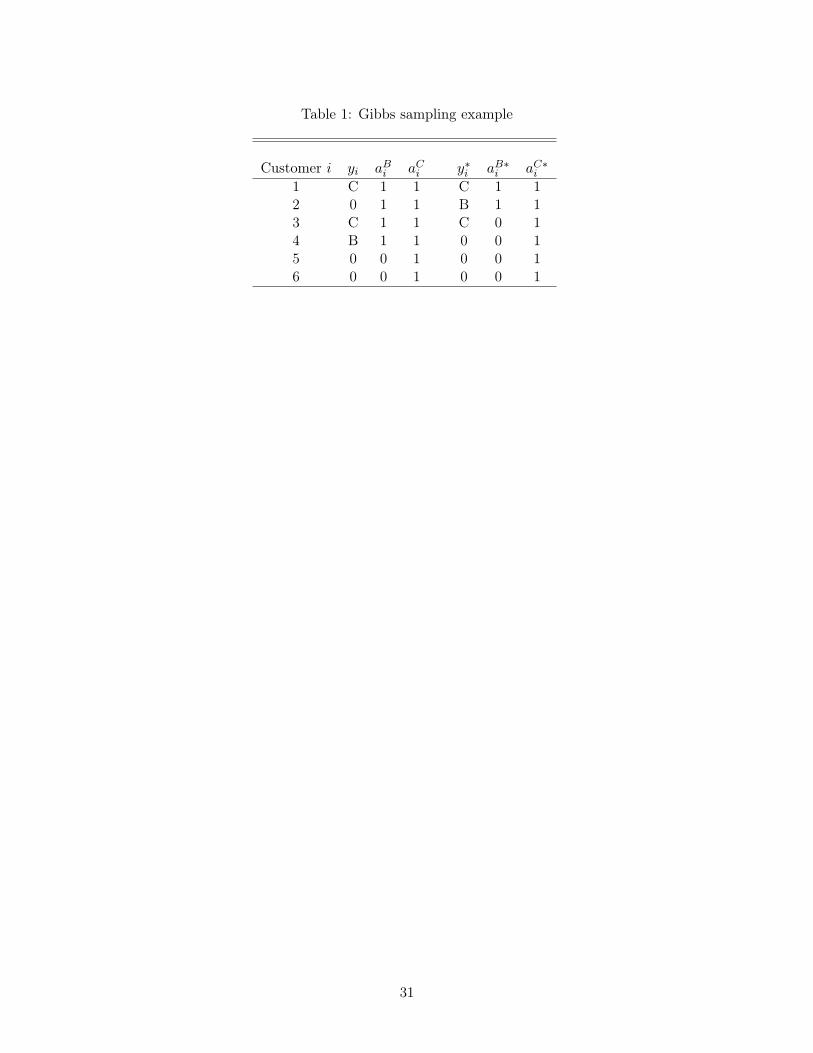
Table 1: Gibbs sampling example

Customer i yi aBi aCi y∗i aB∗i aC∗

i

1 C 1 1 C 1 12 0 1 1 B 1 13 C 1 1 C 0 14 B 1 1 0 0 15 0 0 1 0 0 16 0 0 1 0 0 1

31

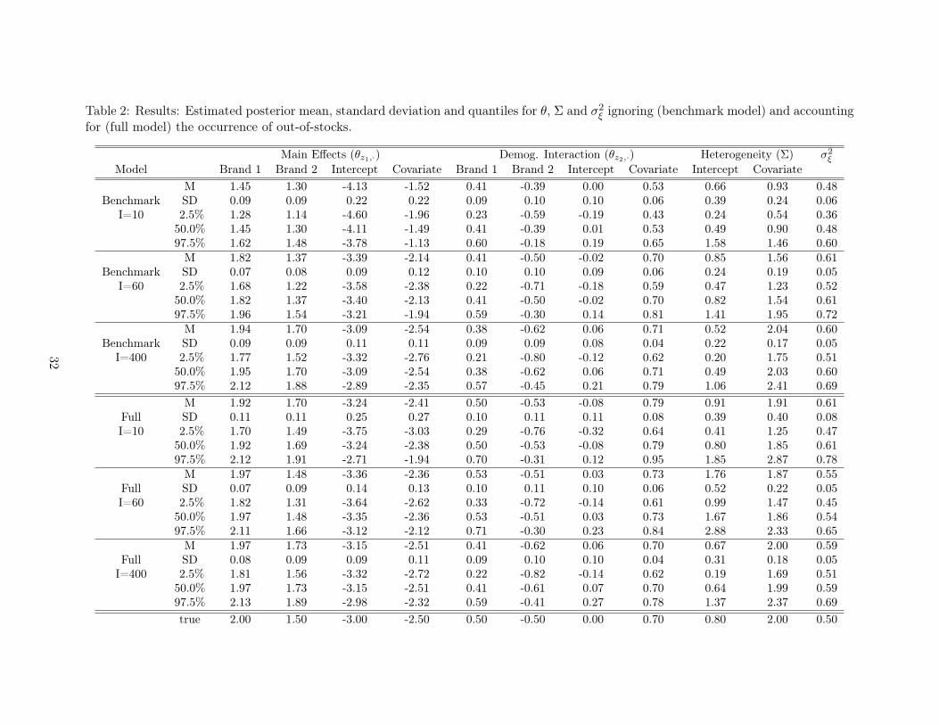
Table 2: Results: Estimated posterior mean, standard deviation and quantiles for �, Σ and �2� ignoring (benchmark model) and accounting

for (full model) the occurrence of out-of-stocks.

Main Effects (�z1,⋅) Demog. Interaction (�z2,⋅) Heterogeneity (Σ) �2

�

Model Brand 1 Brand 2 Intercept Covariate Brand 1 Brand 2 Intercept Covariate Intercept Covariate

M 1.45 1.30 -4.13 -1.52 0.41 -0.39 0.00 0.53 0.66 0.93 0.48Benchmark SD 0.09 0.09 0.22 0.22 0.09 0.10 0.10 0.06 0.39 0.24 0.06

I=10 2.5% 1.28 1.14 -4.60 -1.96 0.23 -0.59 -0.19 0.43 0.24 0.54 0.3650.0% 1.45 1.30 -4.11 -1.49 0.41 -0.39 0.01 0.53 0.49 0.90 0.4897.5% 1.62 1.48 -3.78 -1.13 0.60 -0.18 0.19 0.65 1.58 1.46 0.60

M 1.82 1.37 -3.39 -2.14 0.41 -0.50 -0.02 0.70 0.85 1.56 0.61Benchmark SD 0.07 0.08 0.09 0.12 0.10 0.10 0.09 0.06 0.24 0.19 0.05

I=60 2.5% 1.68 1.22 -3.58 -2.38 0.22 -0.71 -0.18 0.59 0.47 1.23 0.5250.0% 1.82 1.37 -3.40 -2.13 0.41 -0.50 -0.02 0.70 0.82 1.54 0.6197.5% 1.96 1.54 -3.21 -1.94 0.59 -0.30 0.14 0.81 1.41 1.95 0.72

M 1.94 1.70 -3.09 -2.54 0.38 -0.62 0.06 0.71 0.52 2.04 0.60Benchmark SD 0.09 0.09 0.11 0.11 0.09 0.09 0.08 0.04 0.22 0.17 0.05

I=400 2.5% 1.77 1.52 -3.32 -2.76 0.21 -0.80 -0.12 0.62 0.20 1.75 0.5150.0% 1.95 1.70 -3.09 -2.54 0.38 -0.62 0.06 0.71 0.49 2.03 0.6097.5% 2.12 1.88 -2.89 -2.35 0.57 -0.45 0.21 0.79 1.06 2.41 0.69

M 1.92 1.70 -3.24 -2.41 0.50 -0.53 -0.08 0.79 0.91 1.91 0.61Full SD 0.11 0.11 0.25 0.27 0.10 0.11 0.11 0.08 0.39 0.40 0.08I=10 2.5% 1.70 1.49 -3.75 -3.03 0.29 -0.76 -0.32 0.64 0.41 1.25 0.47

50.0% 1.92 1.69 -3.24 -2.38 0.50 -0.53 -0.08 0.79 0.80 1.85 0.6197.5% 2.12 1.91 -2.71 -1.94 0.70 -0.31 0.12 0.95 1.85 2.87 0.78

M 1.97 1.48 -3.36 -2.36 0.53 -0.51 0.03 0.73 1.76 1.87 0.55Full SD 0.07 0.09 0.14 0.13 0.10 0.11 0.10 0.06 0.52 0.22 0.05I=60 2.5% 1.82 1.31 -3.64 -2.62 0.33 -0.72 -0.14 0.61 0.99 1.47 0.45

50.0% 1.97 1.48 -3.35 -2.36 0.53 -0.51 0.03 0.73 1.67 1.86 0.5497.5% 2.11 1.66 -3.12 -2.12 0.71 -0.30 0.23 0.84 2.88 2.33 0.65

M 1.97 1.73 -3.15 -2.51 0.41 -0.62 0.06 0.70 0.67 2.00 0.59Full SD 0.08 0.09 0.09 0.11 0.09 0.10 0.10 0.04 0.31 0.18 0.05

I=400 2.5% 1.81 1.56 -3.32 -2.72 0.22 -0.82 -0.14 0.62 0.19 1.69 0.5150.0% 1.97 1.73 -3.15 -2.51 0.41 -0.61 0.07 0.70 0.64 1.99 0.5997.5% 2.13 1.89 -2.98 -2.32 0.59 -0.41 0.27 0.78 1.37 2.37 0.69

true 2.00 1.50 -3.00 -2.50 0.50 -0.50 0.00 0.70 0.80 2.00 0.50

32

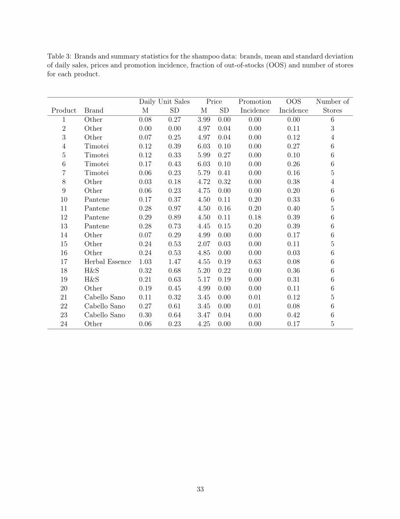
Table 3: Brands and summary statistics for the shampoo data: brands, mean and standard deviationof daily sales, prices and promotion incidence, fraction of out-of-stocks (OOS) and number of storesfor each product.

Daily Unit Sales Price Promotion OOS Number ofProduct Brand M SD M SD Incidence Incidence Stores

1 Other 0.08 0.27 3.99 0.00 0.00 0.00 62 Other 0.00 0.00 4.97 0.04 0.00 0.11 33 Other 0.07 0.25 4.97 0.04 0.00 0.12 44 Timotei 0.12 0.39 6.03 0.10 0.00 0.27 65 Timotei 0.12 0.33 5.99 0.27 0.00 0.10 66 Timotei 0.17 0.43 6.03 0.10 0.00 0.26 67 Timotei 0.06 0.23 5.79 0.41 0.00 0.16 58 Other 0.03 0.18 4.72 0.32 0.00 0.38 49 Other 0.06 0.23 4.75 0.00 0.00 0.20 610 Pantene 0.17 0.37 4.50 0.11 0.20 0.33 611 Pantene 0.28 0.97 4.50 0.16 0.20 0.40 512 Pantene 0.29 0.89 4.50 0.11 0.18 0.39 613 Pantene 0.28 0.73 4.45 0.15 0.20 0.39 614 Other 0.07 0.29 4.99 0.00 0.00 0.17 615 Other 0.24 0.53 2.07 0.03 0.00 0.11 516 Other 0.24 0.53 4.85 0.00 0.00 0.03 617 Herbal Essence 1.03 1.47 4.55 0.19 0.63 0.08 618 H&S 0.32 0.68 5.20 0.22 0.00 0.36 619 H&S 0.21 0.63 5.17 0.19 0.00 0.31 620 Other 0.19 0.45 4.99 0.00 0.00 0.11 621 Cabello Sano 0.11 0.32 3.45 0.00 0.01 0.12 522 Cabello Sano 0.27 0.61 3.45 0.00 0.01 0.08 623 Cabello Sano 0.30 0.64 3.47 0.04 0.00 0.42 624 Other 0.06 0.23 4.25 0.00 0.00 0.17 5

33

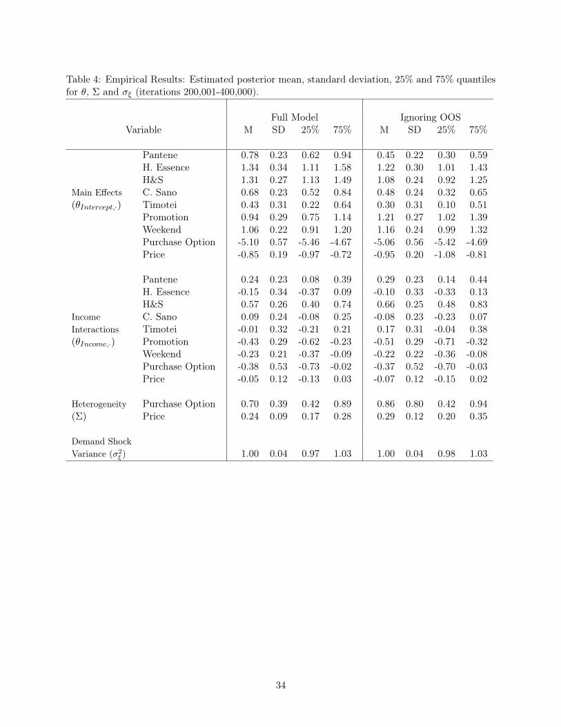
Table 4: Empirical Results: Estimated posterior mean, standard deviation, 25% and 75% quantilesfor �, Σ and �� (iterations 200,001-400,000).

Full Model Ignoring OOSVariable M SD 25% 75% M SD 25% 75%

Pantene 0.78 0.23 0.62 0.94 0.45 0.22 0.30 0.59H. Essence 1.34 0.34 1.11 1.58 1.22 0.30 1.01 1.43H&S 1.31 0.27 1.13 1.49 1.08 0.24 0.92 1.25

Main Effects C. Sano 0.68 0.23 0.52 0.84 0.48 0.24 0.32 0.65(�Intercept,⋅) Timotei 0.43 0.31 0.22 0.64 0.30 0.31 0.10 0.51

Promotion 0.94 0.29 0.75 1.14 1.21 0.27 1.02 1.39Weekend 1.06 0.22 0.91 1.20 1.16 0.24 0.99 1.32Purchase Option -5.10 0.57 -5.46 -4.67 -5.06 0.56 -5.42 -4.69Price -0.85 0.19 -0.97 -0.72 -0.95 0.20 -1.08 -0.81

Pantene 0.24 0.23 0.08 0.39 0.29 0.23 0.14 0.44H. Essence -0.15 0.34 -0.37 0.09 -0.10 0.33 -0.33 0.13H&S 0.57 0.26 0.40 0.74 0.66 0.25 0.48 0.83

Income C. Sano 0.09 0.24 -0.08 0.25 -0.08 0.23 -0.23 0.07Interactions Timotei -0.01 0.32 -0.21 0.21 0.17 0.31 -0.04 0.38(�Income,⋅) Promotion -0.43 0.29 -0.62 -0.23 -0.51 0.29 -0.71 -0.32

Weekend -0.23 0.21 -0.37 -0.09 -0.22 0.22 -0.36 -0.08Purchase Option -0.38 0.53 -0.73 -0.02 -0.37 0.52 -0.70 -0.03Price -0.05 0.12 -0.13 0.03 -0.07 0.12 -0.15 0.02

Heterogeneity Purchase Option 0.70 0.39 0.42 0.89 0.86 0.80 0.42 0.94(Σ) Price 0.24 0.09 0.17 0.28 0.29 0.12 0.20 0.35

Demand Shock

Variance (�2

� ) 1.00 0.04 0.97 1.03 1.00 0.04 0.98 1.03

34

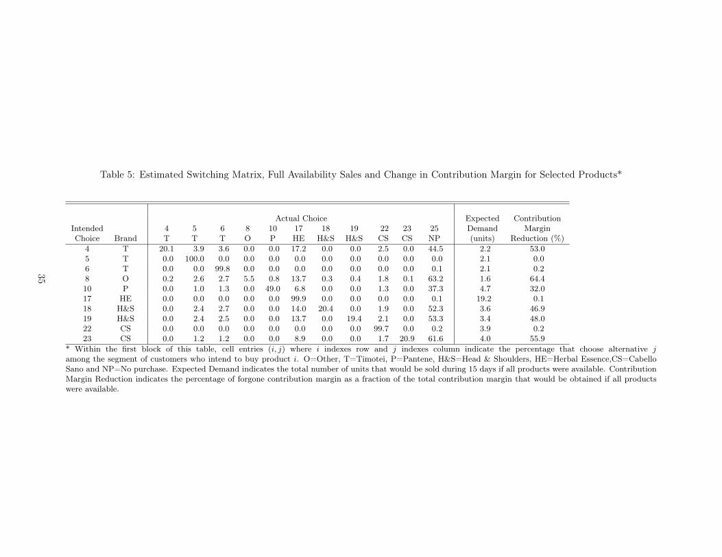
Table 5: Estimated Switching Matrix, Full Availability Sales and Change in Contribution Margin for Selected Products*

Actual Choice Expected ContributionIntended 4 5 6 8 10 17 18 19 22 23 25 Demand MarginChoice Brand T T T O P HE H&S H&S CS CS NP (units) Reduction (%)

4 T 20.1 3.9 3.6 0.0 0.0 17.2 0.0 0.0 2.5 0.0 44.5 2.2 53.05 T 0.0 100.0 0.0 0.0 0.0 0.0 0.0 0.0 0.0 0.0 0.0 2.1 0.06 T 0.0 0.0 99.8 0.0 0.0 0.0 0.0 0.0 0.0 0.0 0.1 2.1 0.28 O 0.2 2.6 2.7 5.5 0.8 13.7 0.3 0.4 1.8 0.1 63.2 1.6 64.410 P 0.0 1.0 1.3 0.0 49.0 6.8 0.0 0.0 1.3 0.0 37.3 4.7 32.017 HE 0.0 0.0 0.0 0.0 0.0 99.9 0.0 0.0 0.0 0.0 0.1 19.2 0.118 H&S 0.0 2.4 2.7 0.0 0.0 14.0 20.4 0.0 1.9 0.0 52.3 3.6 46.919 H&S 0.0 2.4 2.5 0.0 0.0 13.7 0.0 19.4 2.1 0.0 53.3 3.4 48.022 CS 0.0 0.0 0.0 0.0 0.0 0.0 0.0 0.0 99.7 0.0 0.2 3.9 0.223 CS 0.0 1.2 1.2 0.0 0.0 8.9 0.0 0.0 1.7 20.9 61.6 4.0 55.9

* Within the first block of this table, cell entries (i, j) where i indexes row and j indexes column indicate the percentage that choose alternative j

among the segment of customers who intend to buy product i. O=Other, T=Timotei, P=Pantene, H&S=Head & Shoulders, HE=Herbal Essence,CS=CabelloSano and NP=No purchase. Expected Demand indicates the total number of units that would be sold during 15 days if all products were available. ContributionMargin Reduction indicates the percentage of forgone contribution margin as a fraction of the total contribution margin that would be obtained if all productswere available.

35

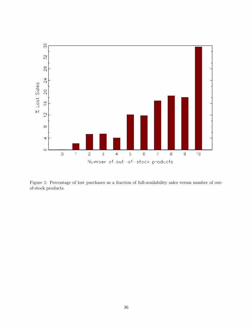
Figure 1: Percentage of lost purchases as a fraction of full-availability sales versus number of out-of-stock products.

36

References

Allenby, G. M., P. E. Rossi. 2003. Bayesian statistics and marketing. Marketing Science 22(3)

304–328.

Anderson, E., G. Fitzsimons, D. Simester. 2006. Measuring and mitigating the cost of stockouts.

Management Science 52(11) 1751–1763.

Andrews, R. L., T. C. Srinivasan. 1995. Studying consideration effects in empirical choice models

using scanner panel data. Journal of Marketing Research 32(February) 30–41.

Anupindi, R., M. Dada, S. Gupta. 1998. Estimation of consumer demand with stock-out based

substitution: An application to vending machine products. Marketing Science 17(4) 406–423.

Ben-Akiva, M. E., S. R. Lerman. 1985. Discrete Choice Analysis: Theory and Application to Travel

Demand . MIT Press.

Berry, S. 1994. Estimating discrete choice models of product differentiation. Rand Journal of

Economics 25(2) 242–262.

Berry, S., J. Levinson, A. Pakes. 1995. Automobile prices in market equilibrium. Econometrica

963(4) 841–890.

Besanko, D., J.-P. Dubé, S. Gupta. 2003. Competitive price discrimination strategies in a vertical

channel using aggregate data. Management Science 49(9) 1121–1138.

Bruno, H., N. Vilcassim. 2008. Structural demand estimation with varying product availability.

Marketing Science 27(6) 1126–1131.

Cachon, Gerard, Marcelo Olivares. 2010. Drivers of finished good inventory in the u.s. automobile

industry. Management Science 56(1) 202–216.

Cachon, Gerard P., Christian Terwiesch. 2005. Matching Supply with Demand . 1st ed. McGraw-Hill,

1221 Avenue of the Americas, New York.

Campo, K., E. Gijsbrechts, P. Nisol. 2003a. The impact of retailer stockouts on whether, how much,

and what to buy. International Journal of Research in Marketing 20(3) 273–286.

37

Campo, K., E. Gijsbrechts, P. Nison. 2003b. Towards understanding consumer response to stock-

outs. Journal of Retailing 72(2).

Chen, Y., S. Yang. 2007. Estimating disaggregate models using aggregate data via augmentation

of individual choice. Journal of Marketing Research 44(November) 596–613.

Chintagunta, P. K., J.-P. Dubé. 2005. Estimating a stockkeeping-unit-level brand choice model

that combines household panel data and store data. Journal of Marketing Research 42(August)

368–379.

Chintagunta, P. K., D. Jain, N. J. Vilcassim. 1991. Investigating heterogeneity in brand preferences

in logit models for panel data. Journal of Marketing Research 28(November) 417–428.

Conlon, C., J. Holland Mortimer. 2009. Demand estimation under incomplete product availability.

Working paper, Harvard University.

DeHoratius, N., A. Raman. 2008. Inventory record inaccuracy: an empirical analysis. Management

Science 54(4) 627–641.

Fader, P., B. Hardie. 1996. Modeling consumer choice among SKUs. Journal of Marketing Research

33(November) 442–452.

Fitzsimons, G. J. 2000. Consumer response to stockouts. Journal of Consumer Research 27(2)

249–266.

Gruen, T.W., D.S. Corsten, S. Bharadwaj. 2002. Retail Out-of-stocks: A Worldwide Examination

of Extent, Causes and Consumer Responses . Grocery Manufacturers of America.

Hauser, J., B. Wernerfelt. 1990. An evaluation cost model of consideration sets. Journal of Consumer

Research 16(March) 393–408.

Jiang, R., P. Manchanda, P. Rossi. 2009. Bayesian analysis of random coefficient logit models using

aggregate data. Journal of Econometrics 149(2) 136–148.

Kalyanam, K., S. Borle, P. Boatwright. 2007. Deconstructing each item’s category contribution.

Marketing Science 26(3) 327–341.

38

Kass, R. E., A. E. Raftery. 1995. Bayes factors. Journal of the American Statistical Association

90(430) 773–795.

Kim, J., G. M. Allenby, P. E. Rossi. 2002. Modeling consumer demand for variety. Marketing

Science 21(3) 229–250.

Kök, A. G., M. L. Fisher. 2007. Demand estimation and assortment optimization under substitution:

Methodology and application. Operations Research 55(6) 1001.

Manchanda, P., P.E. Rossi, P.K. Chintagunta. 2004. Response modeling with nonrandom marketing-

mix variables. Journal of Marketing Research 41(4) 467–478.

Musalem, A., E. T. Bradlow, J. S. Raju. 2008. Who’s got the coupon? Estimating consumer prefer-

ences and coupon usage from aggregate information. Journal of Marketing Research 45(Decem-

ber) 715–730.

Musalem, A., E. T. Bradlow, J. S. Raju. 2009. Bayesian estimation of random-coefficients choice

models using aggregate data. Journal of Applied Econometrics 24(3) 490–516.

O’Connell, Vanessa. 2008. Reversing field, macy’s goes local. Wall Street Journal April 21 B1.

Porteus, Evan L. 2002. Foundations of Stochastic Inventory Theory . Stanford Business Books.

Roberts, J. H., J. M. Lattin. 1991. Development and testing of a model of consideration set com-

position. Journal of Marketing Research 28(4) 429–440.

Rossi, P. E., R. McCulloch, G. M. Allenby. 1996. The value of purchase history data in target

marketing. Marketing Science 15(4) 321–340.

Smith, S. A., N. Agrawal. 2000. Management of Multi-Item Retail Inventory Systems with Demand

Substitution. Operations Research 48(1) 50–64.

Train, K. E. 2003. Discrete Choice Methods with Simulation. Cambridge University Press.

Villas-Boas, J. M., R. S. Winer. 1999. Endogeneity in brand choice models. Management Science

45(10) 1324–1338.

39

Vulcano, G., G. van Ryzin, R. Ratliff. 2008. Estimating primary demand for substitutable products

from sales transaction data. Working paper.

Yang, S., Y. Chen, G.M. Allenby. 2003. Bayesian analysis of simultaneous demand and supply.

Quantitative Marketing and Economics 1(3) 251–275.

Zipkin, P. 2000. Foundations of Inventory Management . McGraw-Hill.

40

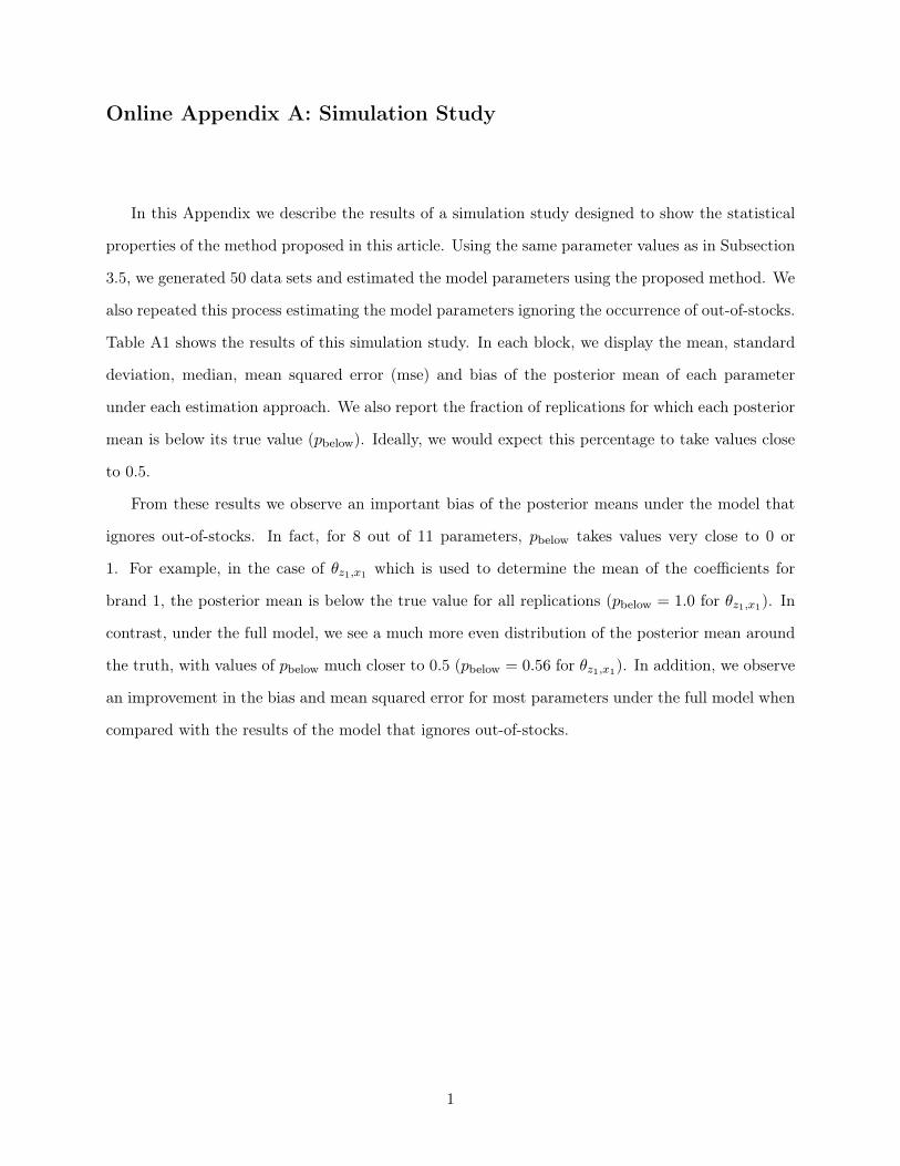
Online Appendix A: Simulation Study

In this Appendix we describe the results of a simulation study designed to show the statistical

properties of the method proposed in this article. Using the same parameter values as in Subsection

3.5, we generated 50 data sets and estimated the model parameters using the proposed method. We

also repeated this process estimating the model parameters ignoring the occurrence of out-of-stocks.

Table A1 shows the results of this simulation study. In each block, we display the mean, standard

deviation, median, mean squared error (mse) and bias of the posterior mean of each parameter

under each estimation approach. We also report the fraction of replications for which each posterior

mean is below its true value (pbelow). Ideally, we would expect this percentage to take values close

to 0.5.

From these results we observe an important bias of the posterior means under the model that

ignores out-of-stocks. In fact, for 8 out of 11 parameters, pbelow takes values very close to 0 or

1. For example, in the case of �z1,x1 which is used to determine the mean of the coefficients for

brand 1, the posterior mean is below the true value for all replications (pbelow = 1.0 for �z1,x1). In

contrast, under the full model, we see a much more even distribution of the posterior mean around

the truth, with values of pbelow much closer to 0.5 (pbelow = 0.56 for �z1,x1). In addition, we observe

an improvement in the bias and mean squared error for most parameters under the full model when

compared with the results of the model that ignores out-of-stocks.

1

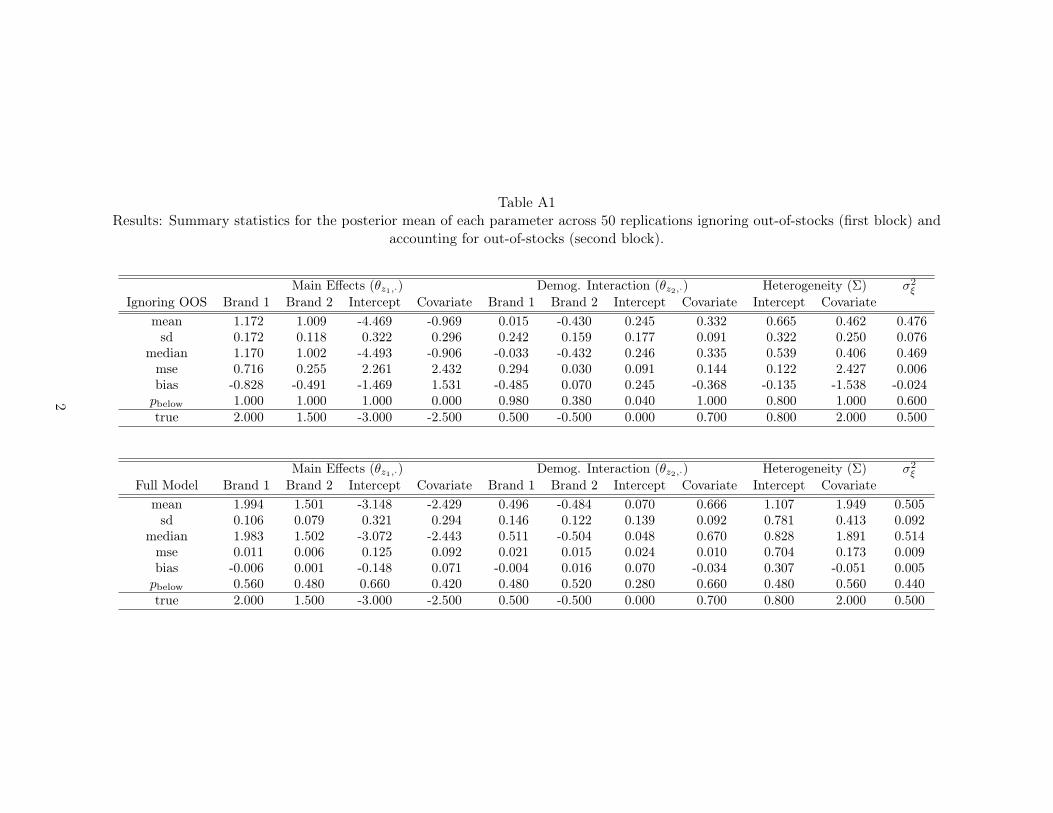
Table A1Results: Summary statistics for the posterior mean of each parameter across 50 replications ignoring out-of-stocks (first block) and

accounting for out-of-stocks (second block).

Main Effects (�z1,⋅) Demog. Interaction (�z2,⋅) Heterogeneity (Σ) �2

�

Ignoring OOS Brand 1 Brand 2 Intercept Covariate Brand 1 Brand 2 Intercept Covariate Intercept Covariate

mean 1.172 1.009 -4.469 -0.969 0.015 -0.430 0.245 0.332 0.665 0.462 0.476sd 0.172 0.118 0.322 0.296 0.242 0.159 0.177 0.091 0.322 0.250 0.076

median 1.170 1.002 -4.493 -0.906 -0.033 -0.432 0.246 0.335 0.539 0.406 0.469mse 0.716 0.255 2.261 2.432 0.294 0.030 0.091 0.144 0.122 2.427 0.006bias -0.828 -0.491 -1.469 1.531 -0.485 0.070 0.245 -0.368 -0.135 -1.538 -0.024pbelow 1.000 1.000 1.000 0.000 0.980 0.380 0.040 1.000 0.800 1.000 0.600true 2.000 1.500 -3.000 -2.500 0.500 -0.500 0.000 0.700 0.800 2.000 0.500

Main Effects (�z1,⋅) Demog. Interaction (�z2,⋅) Heterogeneity (Σ) �2

�

Full Model Brand 1 Brand 2 Intercept Covariate Brand 1 Brand 2 Intercept Covariate Intercept Covariate

mean 1.994 1.501 -3.148 -2.429 0.496 -0.484 0.070 0.666 1.107 1.949 0.505sd 0.106 0.079 0.321 0.294 0.146 0.122 0.139 0.092 0.781 0.413 0.092

median 1.983 1.502 -3.072 -2.443 0.511 -0.504 0.048 0.670 0.828 1.891 0.514mse 0.011 0.006 0.125 0.092 0.021 0.015 0.024 0.010 0.704 0.173 0.009bias -0.006 0.001 -0.148 0.071 -0.004 0.016 0.070 -0.034 0.307 -0.051 0.005pbelow 0.560 0.480 0.660 0.420 0.480 0.520 0.280 0.660 0.480 0.560 0.440true 2.000 1.500 -3.000 -2.500 0.500 -0.500 0.000 0.700 0.800 2.000 0.500

2

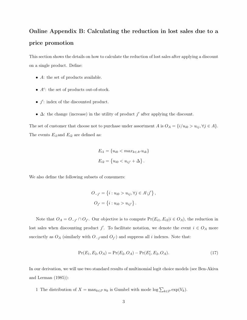
Online Appendix B: Calculating the reduction in lost sales due to a

price promotion

This section shows the details on how to calculate the reduction of lost sales after applying a discount

on a single product. Define:

∙ A: the set of products available.

∙ Ac: the set of products out-of-stock.

∙ j′: index of the discounted product.

∙ Δ: the change (increase) in the utility of product j′ after applying the discount.

The set of customer that choose not to purchase under assortment A is OA = {i/ui0 > uij , ∀j ∈ A}.

The events Ei1and Ei2 are defined as:

Ei1 = {ui0 < maxk∈Acuik}

Ei2 ={

ui0 < uij′ +Δ}

.

We also define the following subsets of consumers:

O−j′ ={

i : ui0 > uij , ∀j ∈ A∖j′}

,

Oj′ ={

i : ui0 > uij′}

.

Note that OA = O−j′ ∩ Oj′ . Our objective is to compute Pr(Ei1, Ei2∣i ∈ OA), the reduction in

lost sales when discounting product j′. To facilitate notation, we denote the event i ∈ OA more

succinctly as OA (similarly with O−j′and Oj′) and suppress all i indexes. Note that:

Pr(E1, E2, OA) = Pr(E2, OA)− Pr(Ec1, E2, OA). (17)

In our derivation, we will use two standard results of multinomial logit choice models (see Ben-Akiva

and Lerman (1985)):

1 The distribution of X = maxk∈P uk is Gumbel with mode log∑

k∈P exp(Vk).

3

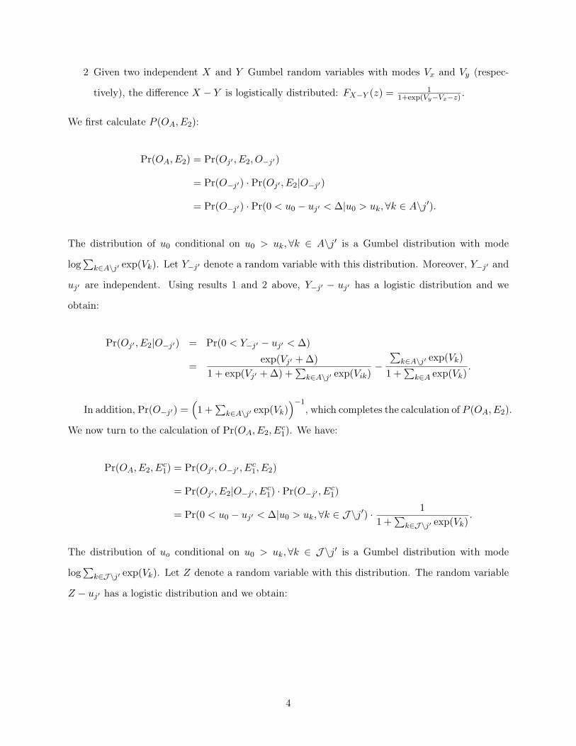
2 Given two independent X and Y Gumbel random variables with modes Vx and Vy (respec-

tively), the difference X − Y is logistically distributed: FX−Y (z) =1

1+exp(Vy−Vx−z) .

We first calculate P (OA, E2):

Pr(OA, E2) = Pr(Oj′ , E2, O−j′)

= Pr(O−j′) ⋅ Pr(Oj′ , E2∣O−j′)

= Pr(O−j′) ⋅ Pr(0 < u0 − uj′ < Δ∣u0 > uk, ∀k ∈ A∖j′).

The distribution of u0 conditional on u0 > uk, ∀k ∈ A∖j′ is a Gumbel distribution with mode

log∑

k∈A∖j′ exp(Vk). Let Y−j′ denote a random variable with this distribution. Moreover, Y−j′ and

uj′ are independent. Using results 1 and 2 above, Y−j′ − uj′ has a logistic distribution and we

obtain:

Pr(Oj′ , E2∣O−j′) = Pr(0 < Y−j′ − uj′ < Δ)

=exp(Vj′ +Δ)

1 + exp(Vj′ +Δ) +∑

k∈A∖j′ exp(Vik)−

∑

k∈A∖j′ exp(Vk)

1 +∑

k∈A exp(Vk).

In addition, Pr(O−j′) =(

1 +∑

k∈A∖j′ exp(Vk))−1

, which completes the calculation of P (OA, E2).

We now turn to the calculation of Pr(OA, E2, Ec1). We have:

Pr(OA, E2, Ec1) = Pr(Oj′ , O−j′ , E

c1, E2)

= Pr(Oj′ , E2∣O−j′ , Ec1) ⋅ Pr(O−j′ , E

c1)

= Pr(0 < u0 − uj′ < Δ∣u0 > uk, ∀k ∈ J ∖j′) ⋅

1

1 +∑

k∈J∖j′ exp(Vk).

The distribution of uo conditional on u0 > uk, ∀k ∈ J ∖j′ is a Gumbel distribution with mode

log∑

k∈J∖j′ exp(Vk). Let Z denote a random variable with this distribution. The random variable

Z − uj′ has a logistic distribution and we obtain:

4

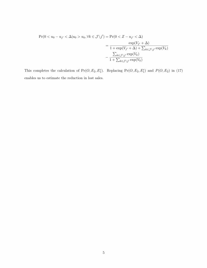
Pr(0 < u0 − uj′ < Δ∣u0 > uk, ∀k ∈ J ∖j′) = Pr(0 < Z − uj′ < Δ)

=exp(Vj′ +Δ)

1 + exp(Vj′ +Δ) +∑

k∈J∖j′ exp(Vk)

−

∑

k∈J∖j′ exp(Vk)

1 +∑

k∈J∖j′ exp(Vk)

This completes the calculation of Pr(O,E2, Ec1). Replacing Pr(O,E2, E

c1) and P (O,E2) in (17)

enables us to estimate the reduction in lost sales.

5