MAR120 - Cantilever Beam LINEAR AND NONLINEAR ANALYSIS OF A CANTILEVER BEAM

MAR120 - Cantilever Beam

LINEAR AND NONLINEARANALYSIS OF A

CANTILEVER BEAM

WS 5 - 2MAR120 - Cantilever Beam

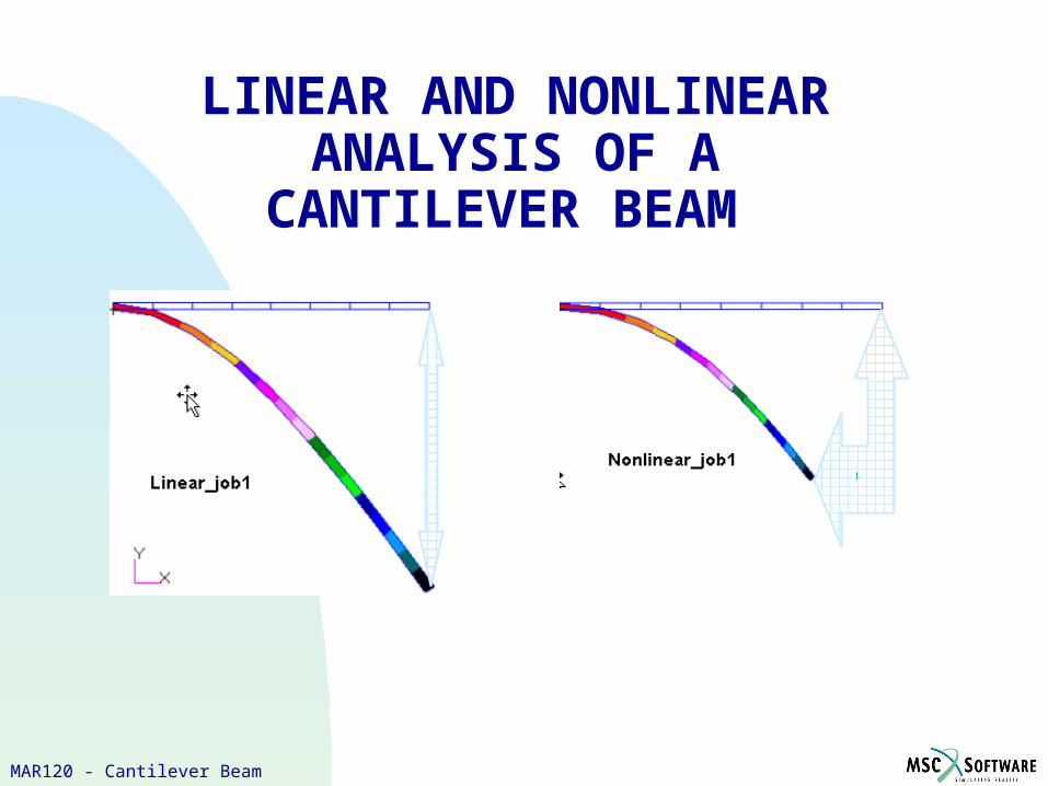
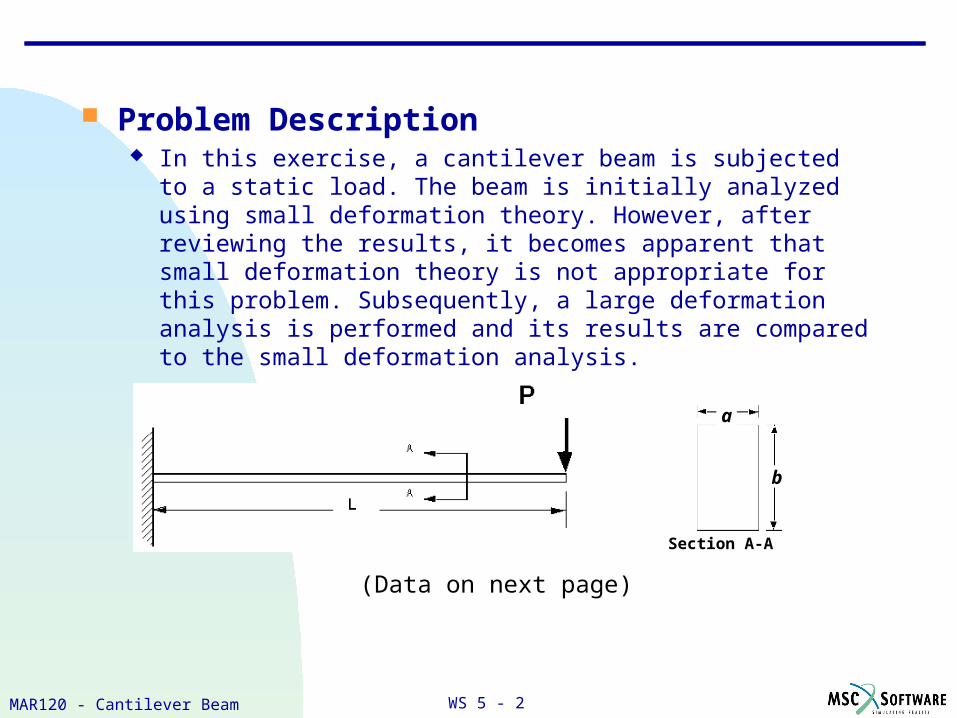
Problem Description In this exercise, a cantilever beam is subjected to a static load. The

beam is initially analyzed using small deformation theory. However, after reviewing the results, it becomes apparent that small deformation theory is not appropriate for this problem. Subsequently, a large deformation analysis is performed and its results are compared to the small deformation analysis.

Section A-A

b

a

(Data on next page)


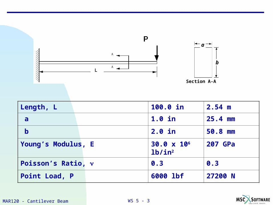
Length, L 100.0 in 2.54 m

a 1.0 in 25.4 mm

b 2.0 in 50.8 mm

Young’s Modulus, E 30.0 x 106 lb/in2 207 GPa

Poisson’s Ratio, 0.3 0.3

Point Load, P 6000 lbf 27200 N

Section A-A

b

a


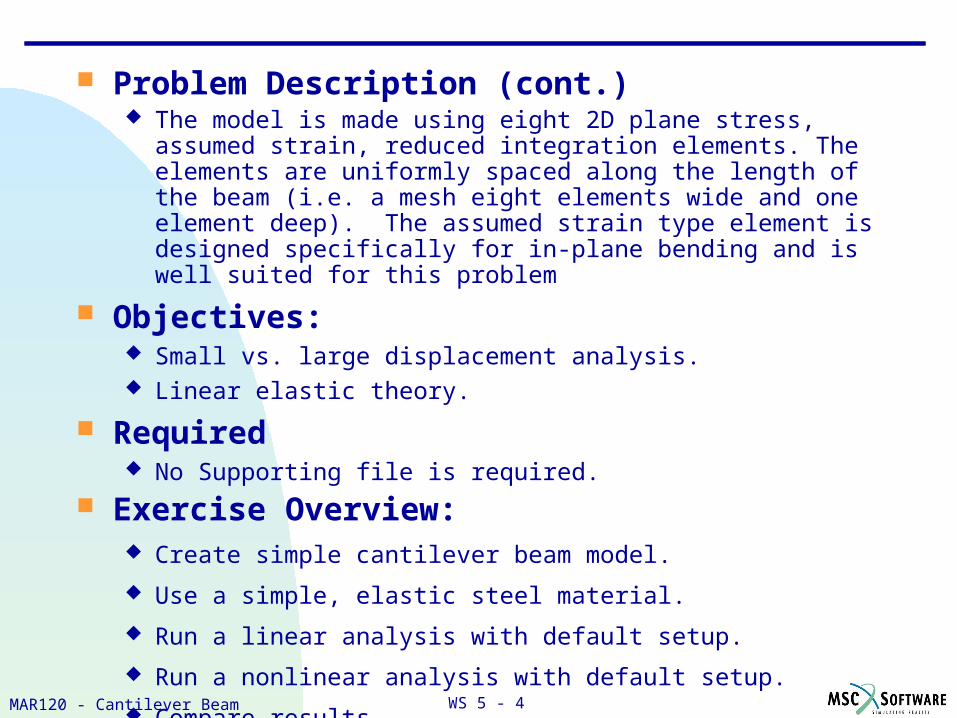
Problem Description (cont.) The model is made using eight 2D plane stress, assumed strain,

reduced integration elements. The elements are uniformly spaced along the length of the beam (i.e. a mesh eight elements wide and one element deep). The assumed strain type element is designed specifically for in-plane bending and is well suited for this problem

Objectives: Small vs. large displacement analysis. Linear elastic theory.

Required No Supporting file is required.

Exercise Overview: Create simple cantilever beam model.

Use a simple, elastic steel material.

Run a linear analysis with default setup.

Run a nonlinear analysis with default setup.

Compare results.


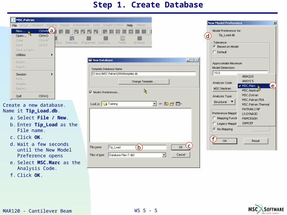
Step 1. Create Database

a

Create a new database. Name it Tip_Load.db.

a. Select File / New.

b. Enter Tip_Load as the File name.

c. Click OK.

d. Wait a few seconds until the New Model Preference opens

e. Select MSC.Marc as the Analysis Code.

f. Click OK.

b c

d

f

e


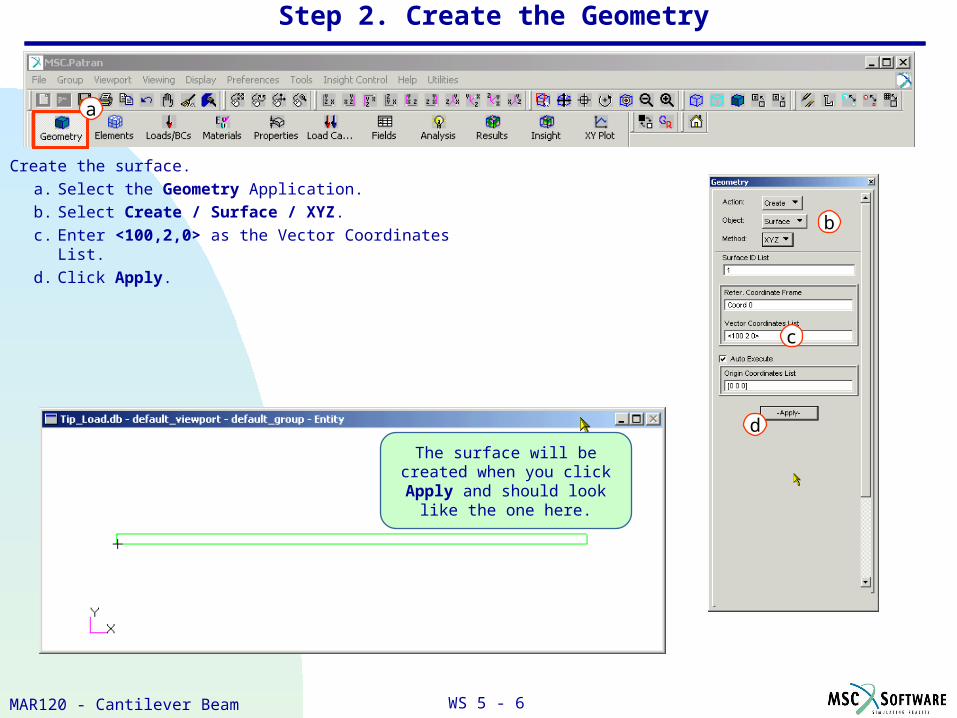
Step 2. Create the Geometry

Create the surface.

a. Select the Geometry Application.

b. Select Create / Surface / XYZ.

c. Enter <100,2,0> as the Vector Coordinates List.

d. Click Apply.

b

c

d

The surface will be created when you click Apply and

should look like the one here.

a


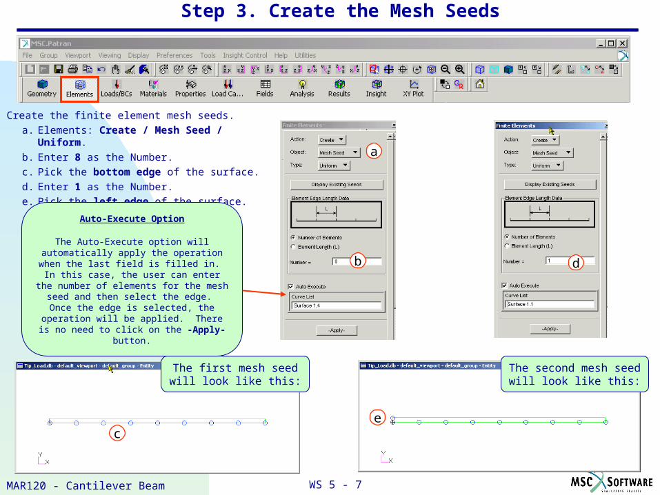
The second mesh seed will look like this:

Step 3. Create the Mesh Seeds

e

d

e

Create the finite element mesh seeds.

a. Elements: Create / Mesh Seed / Uniform.

b. Enter 8 as the Number.

c. Pick the bottom edge of the surface.

d. Enter 1 as the Number.

e. Pick the left edge of the surface.

a

b

The first mesh seed will look like this:

c

Auto-Execute Option

The Auto-Execute option will automatically apply the operation when the last field is filled in. In this case, the user can enter the number of

elements for the mesh seed and then select the edge. Once the edge is selected, the operation

will be applied. There is no need to click on the -Apply- button.


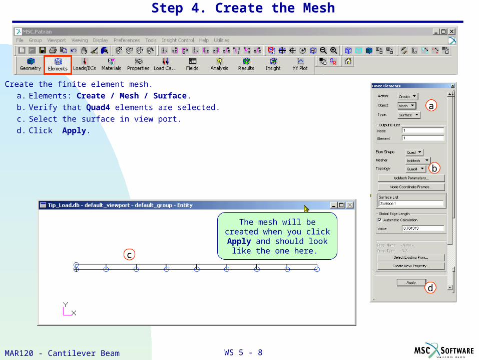
Step 4. Create the Mesh

c

The mesh will be created when you click Apply and

should look like the one here.

Create the finite element mesh.

a. Elements: Create / Mesh / Surface.

b. Verify that Quad4 elements are selected.

c. Select the surface in view port.

d. Click Apply.

b

a

d


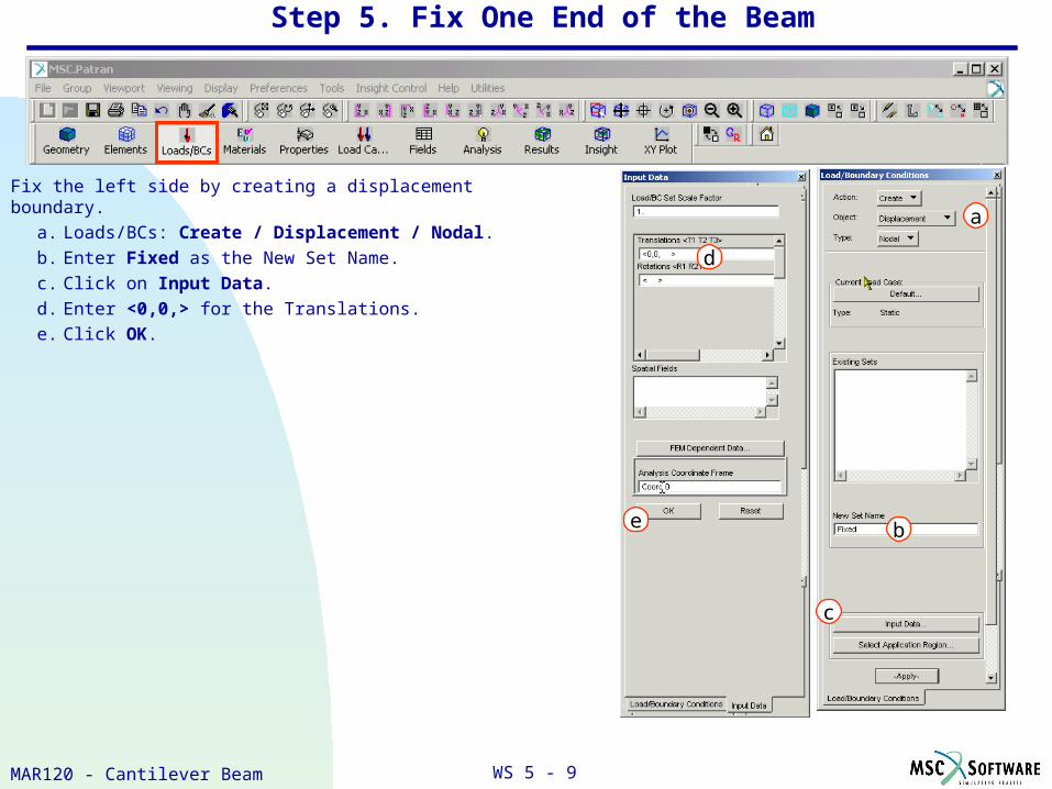
Step 5. Fix One End of the Beam

Fix the left side by creating a displacement boundary.

a. Loads/BCs: Create / Displacement / Nodal.

b. Enter Fixed as the New Set Name.

c. Click on Input Data.

d. Enter <0,0,> for the Translations.

e. Click OK.

d

e

a

b

c


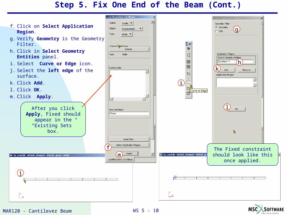
f. Click on Select Application Region.

g. Verify Geometry is the Geometry Filter.

h. Click in Select Geometry Entities panel.

i. Select Curve or Edge icon.

j. Select the left edge of the surface.

k. Click Add.

l. Click OK.

m. Click Apply.

Step 5. Fix One End of the Beam (Cont.)

mf

After you click Apply, Fixed should appear in the

“Existing Sets” box.

g

h

i

j

k

l

The Fixed constraint should look like this once applied.


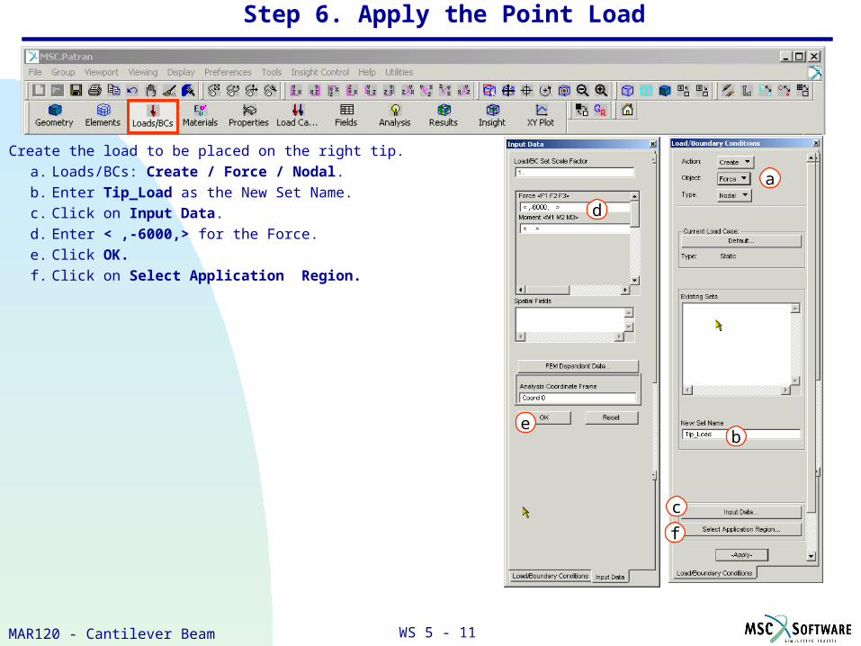
Step 6. Apply the Point Load

Create the load to be placed on the right tip.

a. Loads/BCs: Create / Force / Nodal.

b. Enter Tip_Load as the New Set Name.

c. Click on Input Data.

d. Enter < ,-6000,> for the Force.

e. Click OK.

f. Click on Select Application Region.

d

e

a

b

c

f


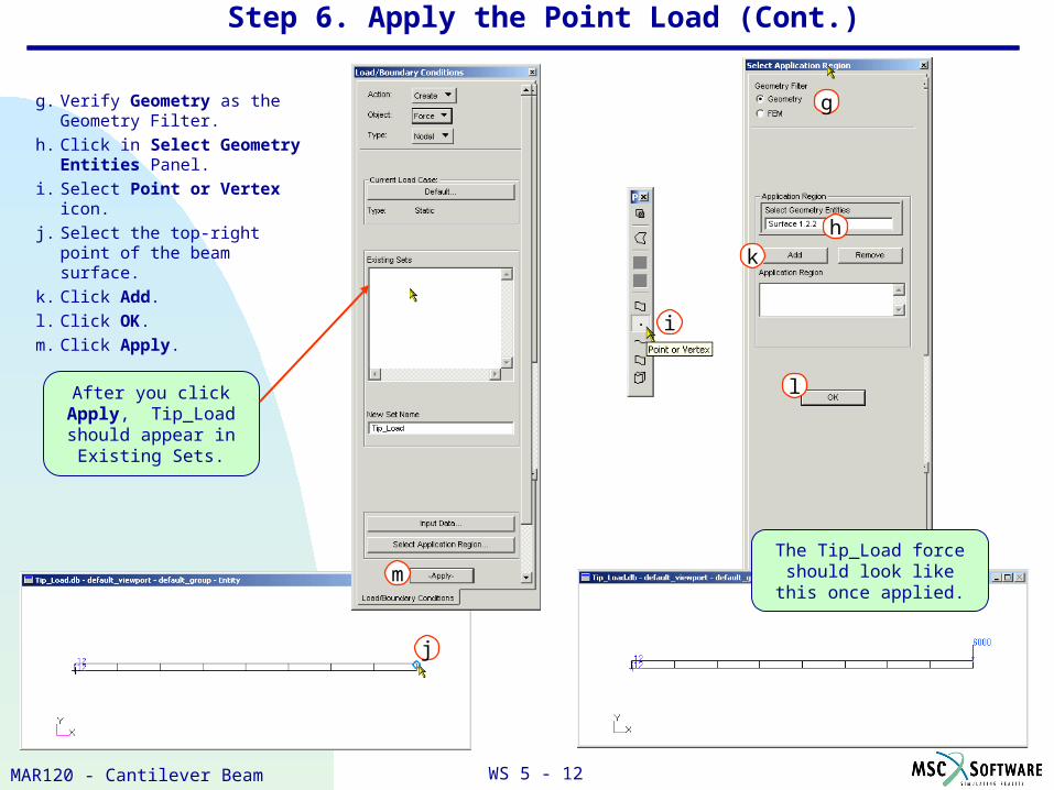
g. Verify Geometry as the Geometry Filter.

h. Click in Select Geometry Entities Panel.

i. Select Point or Vertex icon.

j. Select the top-right point of the beam surface.

k. Click Add.

l. Click OK.

m. Click Apply.

Step 6. Apply the Point Load (Cont.)

j

m

k

l

h

g

i

j

After you click Apply, Tip_Load should

appear in Existing Sets.

The Tip_Load force should look like this once applied.


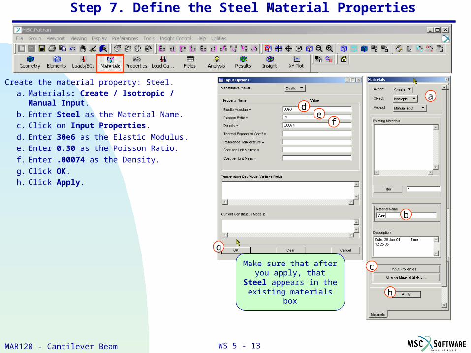
Step 7. Define the Steel Material Properties

de

g

f

Make sure that after you apply, that Steel appears in the existing materials

box

Create the material property: Steel.

a. Materials: Create / Isotropic / Manual Input.

b. Enter Steel as the Material Name.

c. Click on Input Properties.

d. Enter 30e6 as the Elastic Modulus.

e. Enter 0.30 as the Poisson Ratio.

f. Enter .00074 as the Density.

g. Click OK.

h. Click Apply.

a

b

c

h


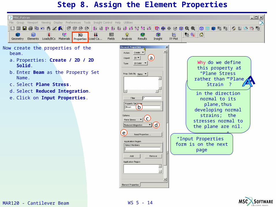
The test specimen is free to contract in the direction

normal to its plane,thus developing normal strains; the stresses normal to the

plane are nil.

Why do we define this property as “Plane Stress” rather than “Plane Strain” ?

Step 8. Assign the Element Properties

“Input Properties” form is on the next page

Now create the properties of the beam.

a. Properties: Create / 2D / 2D Solid.

b. Enter Beam as the Property Set Name.

c. Select Plane Stress.

d. Select Reduced Integration.

e. Click on Input Properties.

a

b

cd

e


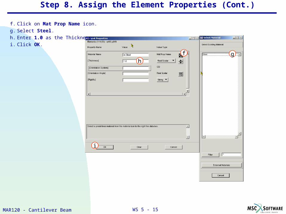
f. Click on Mat Prop Name icon.

g. Select Steel.

h. Enter 1.0 as the Thickness.

i. Click OK.

gf

h

i

Step 8. Assign the Element Properties (Cont.)


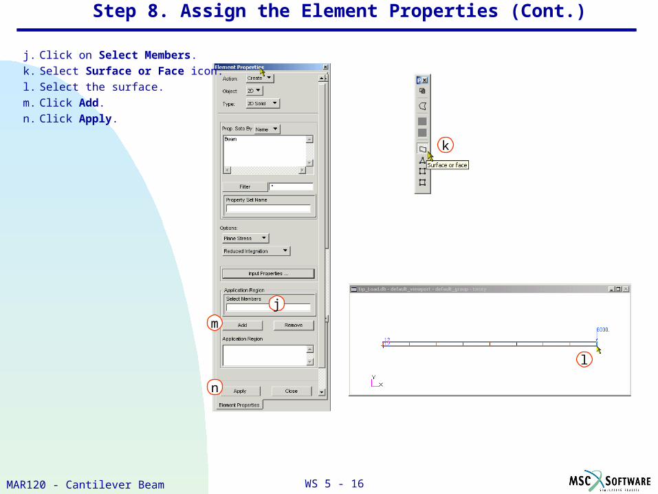
Step 8. Assign the Element Properties (Cont.)

j. Click on Select Members.

k. Select Surface or Face icon.

l. Select the surface.

m. Click Add.

n. Click Apply.

k

j

l

n

m


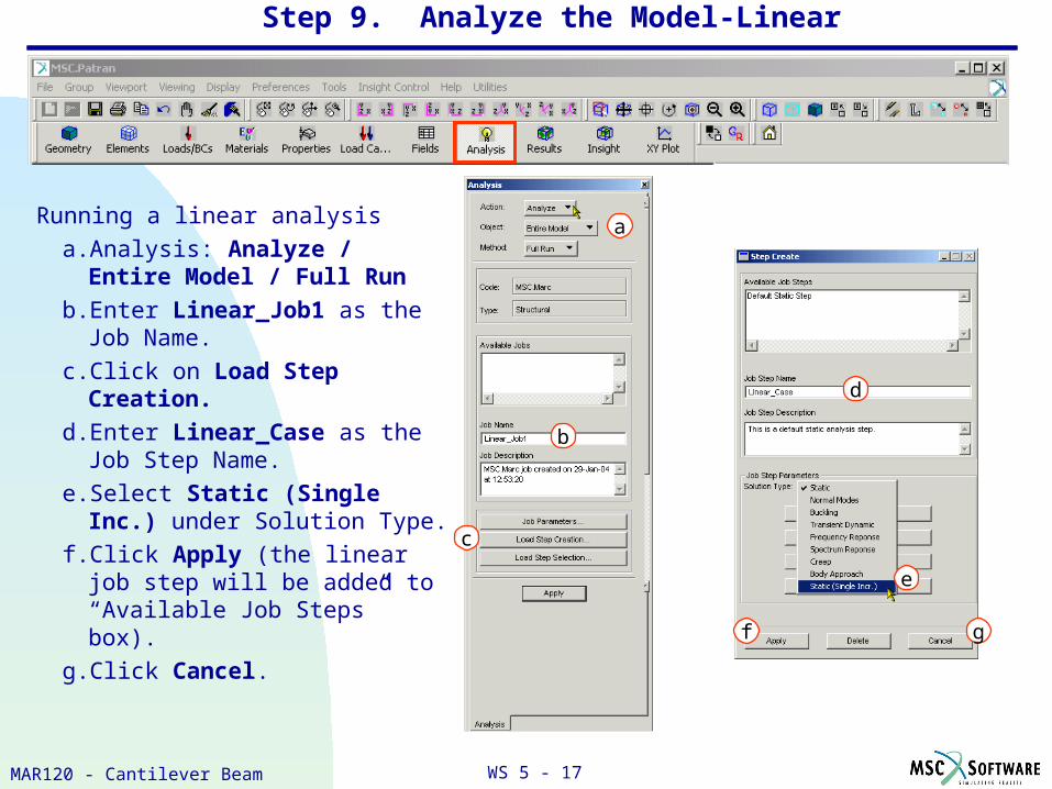
Step 9. Analyze the Model-Linear

Running a linear analysis

a. Analysis: Analyze / Entire Model / Full Run

b. Enter Linear_Job1 as the Job Name.

c. Click on Load Step Creation.

d. Enter Linear_Case as the Job Step Name.

e. Select Static (Single Inc.) under Solution Type.

f. Click Apply (the linear job step will be added to “Available Job Steps” box).

g. Click Cancel.

a

b

c

e

f

d

g


l

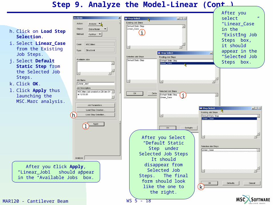
ih. Click on Load Step Selection.

i. Select Linear_Case from the Existing Job Steps.

j. Select Default Static Step from the Selected Job Steps.

k. Click OK.

l. Click Apply thus launching the MSC.Marc analysis.

j

k

Step 9. Analyze the Model-Linear (Cont.)

After you click Apply, “Linear_Job1” should appear in the “Available Jobs”

box.

After you Select “Default Static Step” under

Selected Job Steps It should disappear from

Selected Job Steps. The final form should look like

the one to the right.

After you select “Linear_Case” in the “Existing Job Steps” box, it should appear in the “Selected Job Steps” box.

h


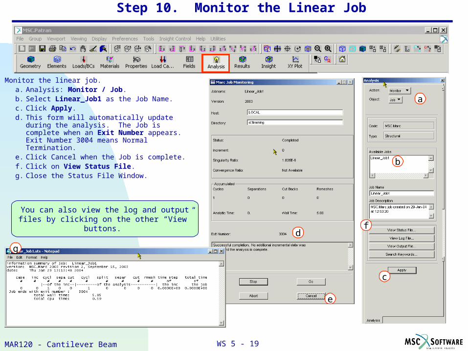
Step 10. Monitor the Linear Job

Monitor the linear job.a. Analysis: Monitor / Job.b. Select Linear_Job1 as the Job Name.c. Click Apply.d. This form will automatically update during the

analysis. The Job is complete when an Exit Number appears. Exit Number 3004 means Normal Termination.

e. Click Cancel when the Job is complete.f. Click on View Status File.g. Close the Status File Window.

You can also view the log and output files by clicking on the other “View” buttons.

a

b

c

d

e

f

g


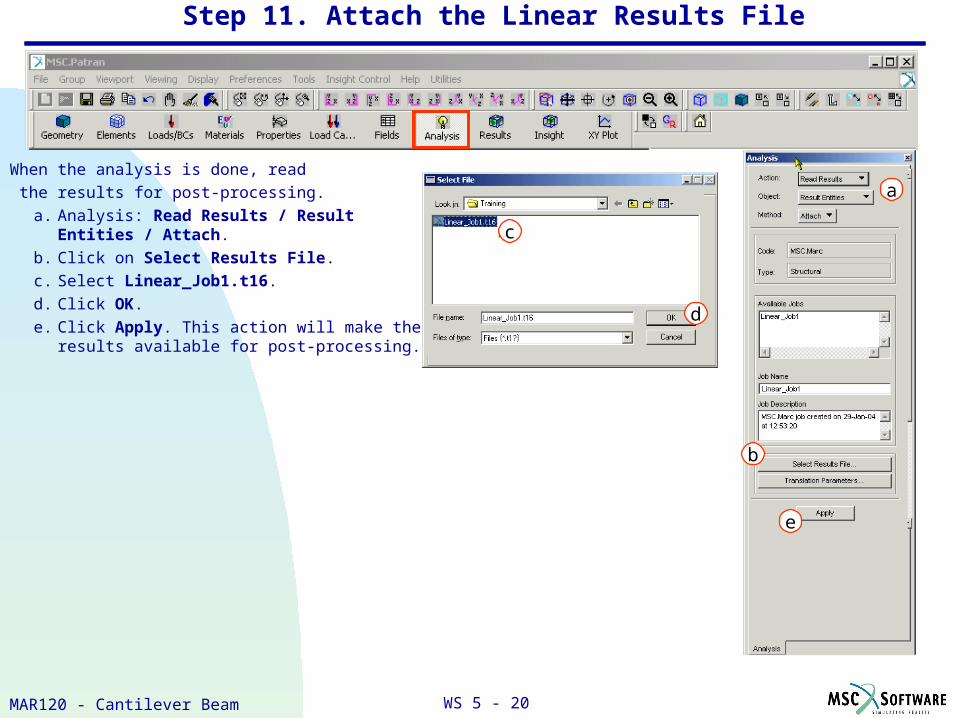
Step 11. Attach the Linear Results File

When the analysis is done, read

the results for post-processing.

a. Analysis: Read Results / Result Entities / Attach.

b. Click on Select Results File.

c. Select Linear_Job1.t16.

d. Click OK.

e. Click Apply. This action will make the results available for post-processing.

a

b

e

c

d


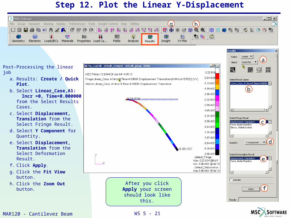
Step 12. Plot the Linear Y-Displacement

Post-Processing the linear job

a. Results: Create / Quick Plot.

b. Select Linear_Case,A1: Incr =0, Time=0.000000 from the Select Results Cases.

c. Select Displacement, Translation from the Select Fringe Result.

d. Select Y Component for Quantity.

e. Select Displacement, Translation from the Select Deformation Result.

f. Click Apply.

g. Click the Fit View button.

h. Click the Zoom Out button.

a

b

c

d

e

f

hg

After you click Apply your screen should look like this.


000,900

21

100000,66

6

100211030

100000,6

4

3

2max

2max

max

36

3

max

3

33

max

ba

PL

I

bM

U

abE

PL

EI

PLU

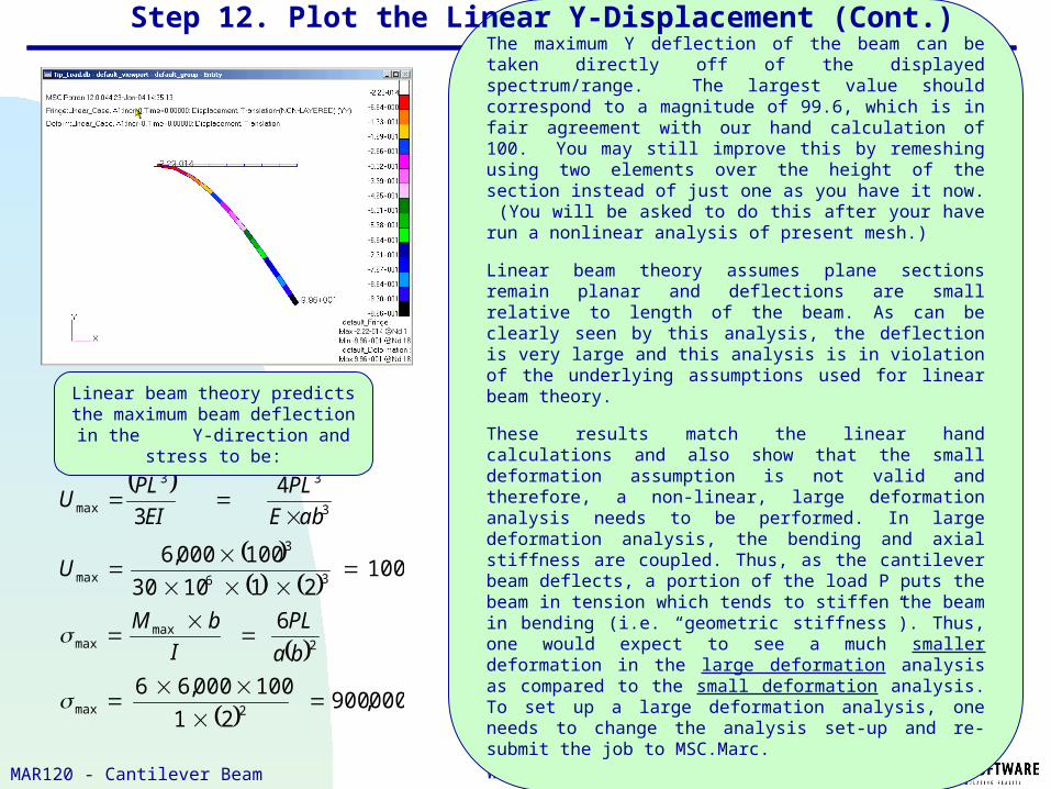
The maximum Y deflection of the beam can be taken directly off of the displayed spectrum/range. The largest value should correspond to a magnitude of 99.6, which is in fair agreement with our hand calculation of 100. You may still improve this by remeshing using two elements over the height of the section instead of just one as you have it now. (You will be asked to do this after your have run a nonlinear analysis of present mesh.)

Linear beam theory assumes plane sections remain planar and deflections are small relative to length of the beam. As can be clearly seen by this analysis, the deflection is very large and this analysis is in violation of the underlying assumptions used for linear beam theory.

These results match the linear hand calculations and also show that the small deformation assumption is not valid and therefore, a non-linear, large deformation analysis needs to be performed. In large deformation analysis, the bending and axial stiffness are coupled. Thus, as the cantilever beam deflects, a portion of the load P puts the beam in tension which tends to stiffen the beam in bending (i.e. “geometric stiffness”). Thus, one would expect to see a much smaller deformation in the large deformation analysis as compared to the small deformation analysis. To set up a large deformation analysis, one needs to change the analysis set-up and re-submit the job to MSC.Marc.

Linear beam theory predicts the maximum beam deflection in the

Y-direction and stress to be:

Step 12. Plot the Linear Y-Displacement (Cont.)


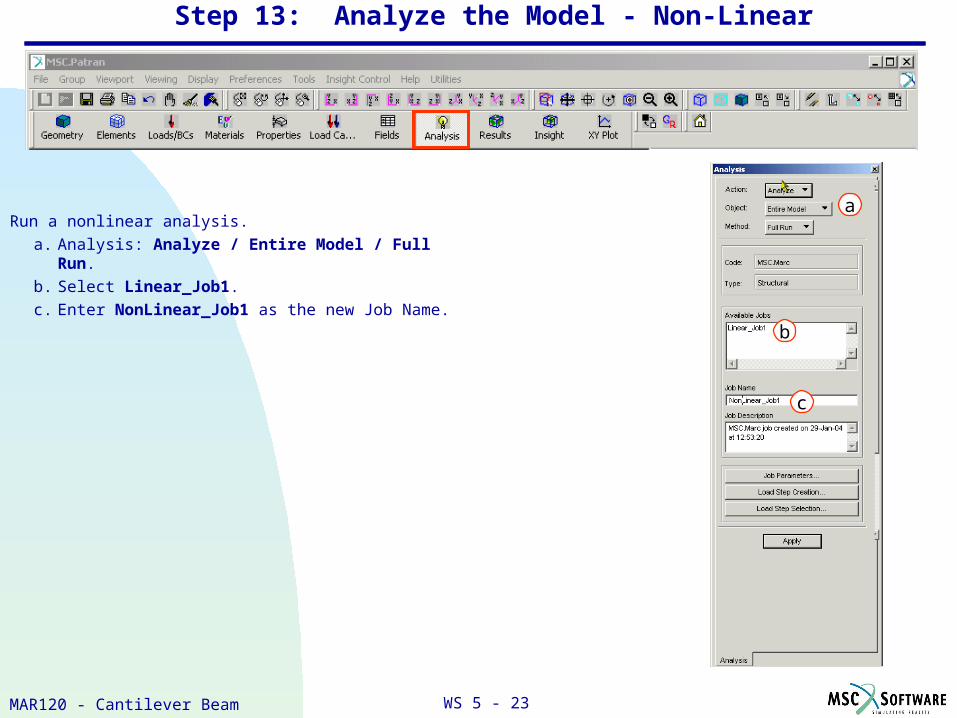
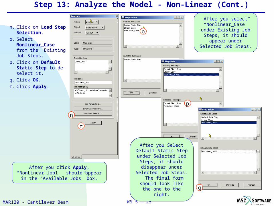
Step 13: Analyze the Model - Non-Linear

Run a nonlinear analysis.

a. Analysis: Analyze / Entire Model / Full Run.

b. Select Linear_Job1.

c. Enter NonLinear_Job1 as the new Job Name.

a

b

c


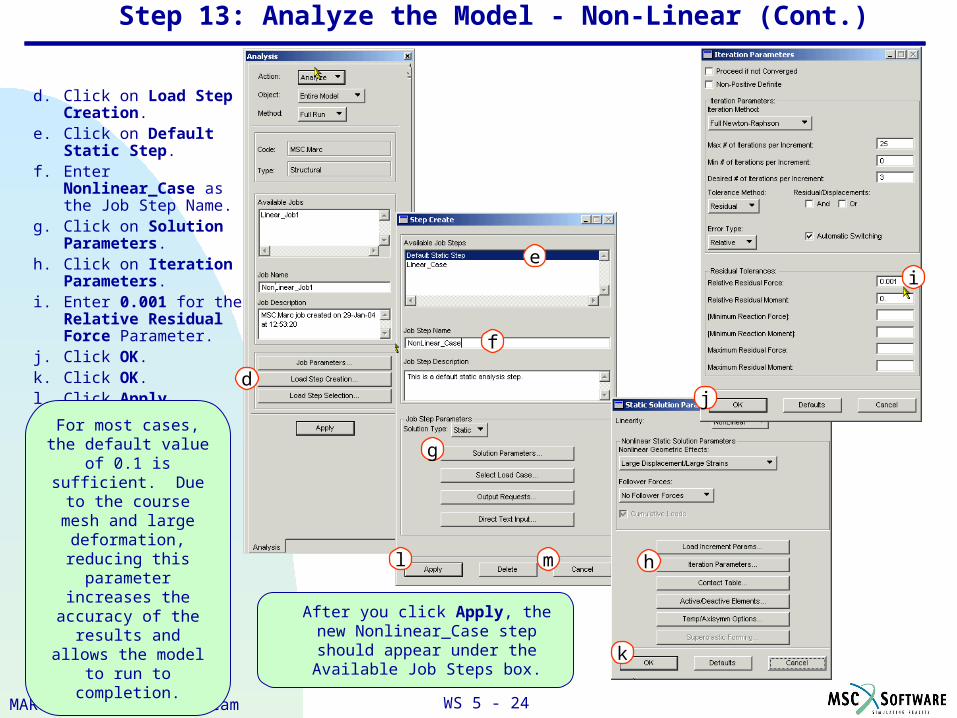
d. Click on Load Step Creation.

e. Click on Default Static Step.

f. Enter Nonlinear_Case as the Job Step Name.

g. Click on Solution Parameters.

h. Click on Iteration Parameters.

i. Enter 0.001 for the Relative Residual Force Parameter.

j. Click OK.k. Click OK.l. Click Apply.m. Click Cancel.

k

d

e

f

g

h

For most cases, the default value of 0.1 is sufficient. Due to the

course mesh and large deformation, reducing

this parameter increases the accuracy

of the results and allows the model to run

to completion. k

l

Step 13: Analyze the Model - Non-Linear (Cont.)

After you click Apply, the new Nonlinear_Case step should appear under the Available Job Steps box.

i

j

m


n. Click on Load Step Selection.

o. Select Nonlinear_Case from the Existing Job Steps.

p. Click on Default Static Step to de-select it.

q. Click OK.

r. Click Apply.

Step 13: Analyze the Model - Non-Linear (Cont.)

n

o

p

q

r

After you Select Default Static Step under

Selected Job Steps, it should disappear under

Selected Job Steps. The final form should look like

the one to the right.

After you select “Nonlinear_Case” under

Existing Job Steps, it should appear under Selected Job Steps.

After you click Apply, “NonLinear_Job1” should appear in the “Available Jobs” box.


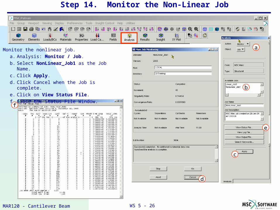
Step 14. Monitor the Non-Linear Job

Monitor the nonlinear job.

a. Analysis: Monitor / Job.

b. Select NonLinear_Job1 as the Job Name.

c. Click Apply.

d. Click Cancel when the Job is complete.

e. Click on View Status File.

f. Close the Status File Window. b

c

a

d

e

f


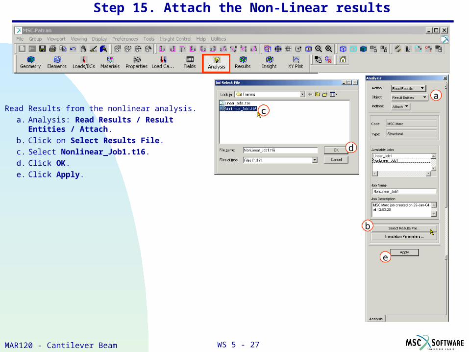
Step 15. Attach the Non-Linear results

a

b

c

d

e

Read Results from the nonlinear analysis.

a. Analysis: Read Results / Result Entities / Attach.

b. Click on Select Results File.

c. Select Nonlinear_Job1.t16.

d. Click OK.

e. Click Apply.


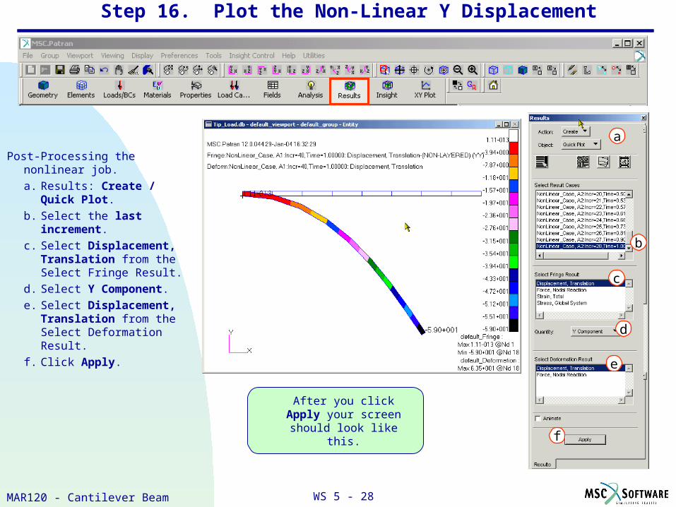
Step 16. Plot the Non-Linear Y Displacement

After you click Apply your screen should look like this.

Post-Processing the nonlinear job.

a. Results: Create / Quick Plot.

b. Select the last increment.

c. Select Displacement, Translation from the Select Fringe Result.

d. Select Y Component.

e. Select Displacement, Translation from the Select Deformation Result.

f. Click Apply.

b

a

c

d

e

f


Step 17. Compare Your Results

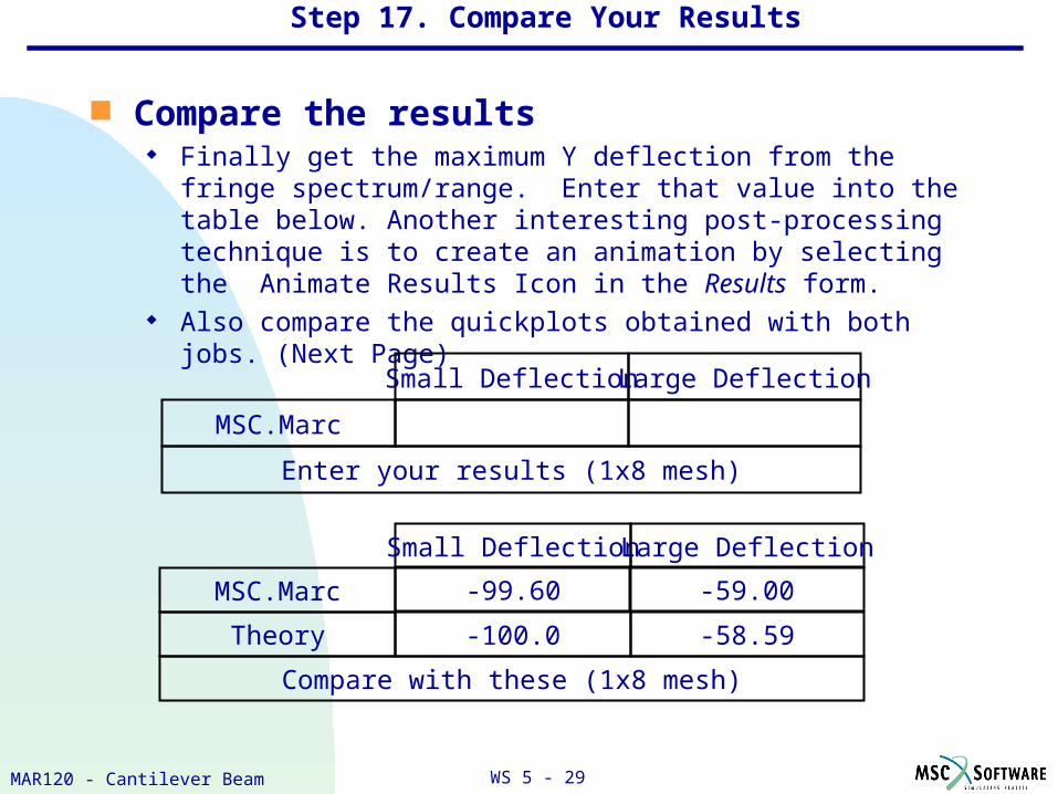
Compare the results Finally get the maximum Y deflection from the fringe

spectrum/range. Enter that value into the table below. Another interesting post-processing technique is to create an animation by selecting the Animate Results Icon in the Results form.

Also compare the quickplots obtained with both jobs. (Next Page)

MSC.Marc

Small Deflection Large Deflection

Enter your results (1x8 mesh)

MSC.Marc

Theory -100.0 -58.59

Small Deflection Large Deflection

-99.60 -59.00

Compare with these (1x8 mesh)


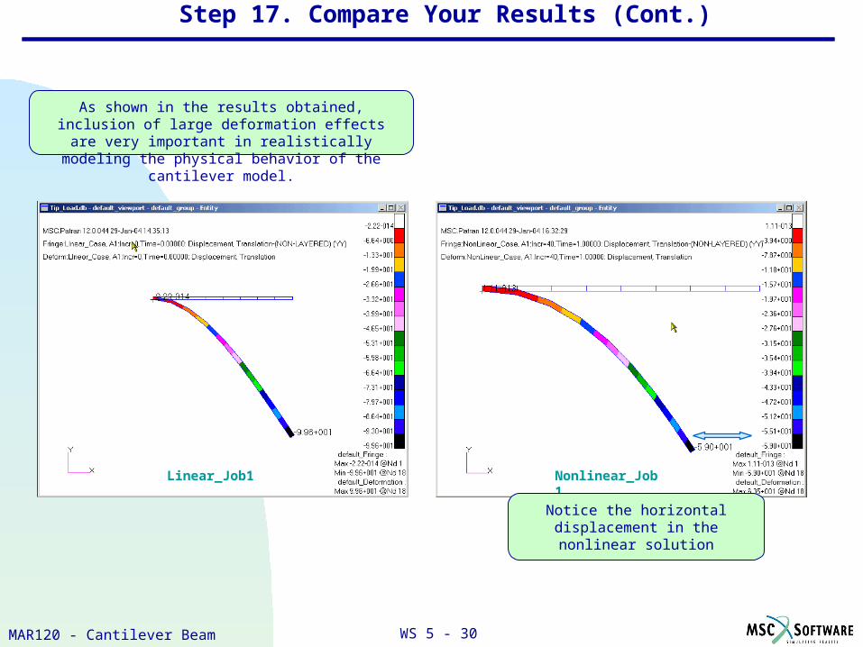
As shown in the results obtained, inclusion of large deformation effects are very important in realistically

modeling the physical behavior of the cantilever model.

Nonlinear_Job1Linear_Job1

Notice the horizontal displacement in the nonlinear solution

Step 17. Compare Your Results (Cont.)


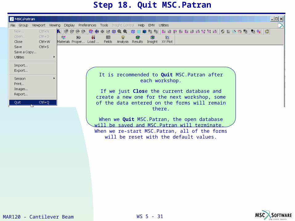
Step 18. Quit MSC.Patran

It is recommended to Quit MSC.Patran after each workshop.

If we just Close the current database and create a new one for the next workshop, some of the data entered on the forms will

remain there.

When we Quit MSC.Patran, the open database will be saved and MSC.Patran will terminate. When we re-start MSC.Patran,

all of the forms will be reset with the default values.


Various Mesh Results

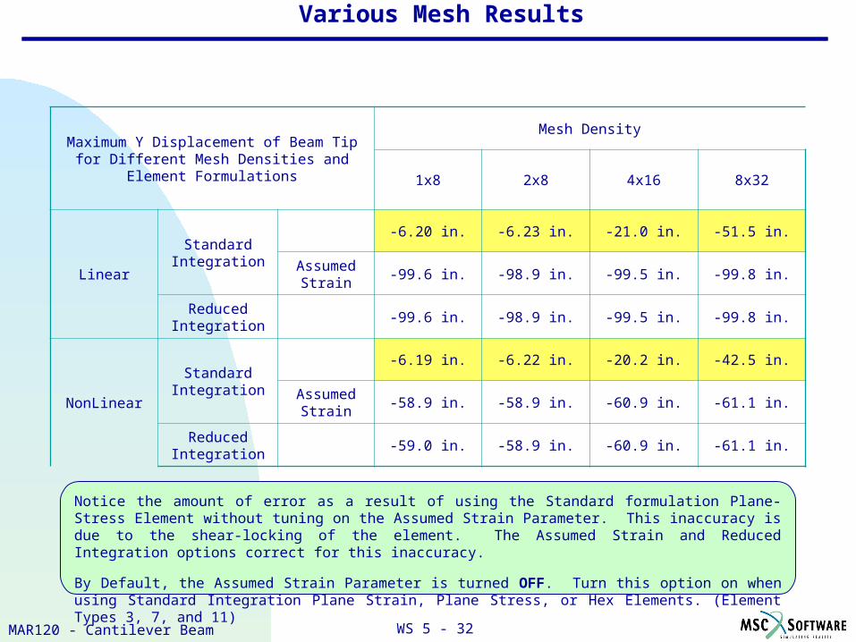
Maximum Y Displacement of Beam Tip for Different Mesh Densities and Element

Formulations

Mesh Density

1x8 2x8 4x16 8x32

Linear

Standard Integration

-6.20 in. -6.23 in. -21.0 in. -51.5 in.

Assumed Strain

-99.6 in. -98.9 in. -99.5 in. -99.8 in.

Reduced Integration

-99.6 in. -98.9 in. -99.5 in. -99.8 in.

NonLinear

Standard Integration

-6.19 in. -6.22 in. -20.2 in. -42.5 in.

Assumed Strain

-58.9 in. -58.9 in. -60.9 in. -61.1 in.

Reduced Integration

-59.0 in. -58.9 in. -60.9 in. -61.1 in.

Notice the amount of error as a result of using the Standard formulation Plane-Stress Element without tuning on the Assumed Strain Parameter. This inaccuracy is due to the shear-locking of the element. The Assumed Strain and Reduced Integration options correct for this inaccuracy.

By Default, the Assumed Strain Parameter is turned OFF. Turn this option on when using Standard Integration Plane Strain, Plane Stress, or Hex Elements. (Element Types 3, 7, and 11)

Documents

MAR120 - Cantilever Beam LINEAR AND NONLINEAR ANALYSIS OF A CANTILEVER BEAM