Embed Size (px)
Citation preview

Forsknings- Og Innovationsstyrelsen
Report
April 2013
Structural Design of
Wave Energy Devices
Long-term Wave Prediction
Deliverable D1.1

11804965 SDWED Long-term Wave Prediction D1.1/jts/mgo/ybr/pot – 09Apr13
This project has been prepared under the
DHI Business Management System
certified by DNV to be in compliance with
ISO 9001: Quality Management System
DHI• Agern Allé 5 • 2970 Hørsholm• Denmark• Telephone: 0045 4516 9200 • Telefax: 0045 4516 9292 • [email protected]• www.dhigroup.com
Structural Design of
Wave Energy Devices
Long-term Wave Prediction
Deliverable D1.1
Prepared for Forsknings- Og Innovationsstyrelsen
Represented by Assoc.Prof Dr Jens Peter Kofoed, Aalborg University
(Principal Investigator, SDWED project)
Project manager Jacob Viborg Tornfeldt Sørensen
Authors Erwan Tacher, Jacob V Tornfeldt Sørensen, Maziar Golestani
Reviewer Maziar Golestani
Approver Jacob V Tornfeldt Sørensen
Project number 11804965
Approval date 10 April 2013
Revision Final: 1.0
Classification Restricted

11804965 SDWED Long-term Wave Prediction D1.1/jts/mgo/ybr/pot – 09Apr13
i
CONTENTS
1 Introduction and Summary ......................................................................................... 1
2 Methodology ................................................................................................................ 3 2.1 Spectral wave modelling ................................................................................................................ 3 2.1.1 MIKE 21 SW ................................................................................................................................... 3
3 Hindcast Data .............................................................................................................. 5 3.1 Bathymetry ..................................................................................................................................... 5 3.2 Wind ............................................................................................................................................... 5 3.3 Water levels ................................................................................................................................... 6 3.4 Boundary conditions ...................................................................................................................... 6 3.5 Validation data ............................................................................................................................... 6
4 Spectral Wave Model Set-up....................................................................................... 7 4.1 Model mesh .................................................................................................................................... 7 4.2 Model set-up .................................................................................................................................. 8
5 Calibration and Validation Results............................................................................. 9 5.1 Validation ..................................................................................................................................... 11
6 Spectral Data, Wave Power Maps ............................................................................ 13 6.1 Spectra ......................................................................................................................................... 16 6.1.1 Extreme events ............................................................................................................................ 16 6.1.2 Production of sea states .............................................................................................................. 17 6.1.3 Wave parameter distribution near Hanstholm ............................................................................. 18 6.2 Wave power maps ....................................................................................................................... 20 6.3 Data distribution ........................................................................................................................... 20
7 Summary .................................................................................................................... 23
8 References ................................................................................................................. 25
APPENDICES
APPENDIX A General Description of the QI
APPENDIX B The Full 30-year Scatter Diagrams for Points P1 to P7
ii 11804965 SDWED Long-term Wave Prediction D1.1/jts/mgo/ybr/pot – 09Apr13
FIGURES
Figure 3.1 Coverage of DHI’s NSBS flow model ............................................................................................ 6 Figure 4.1 Mesh of the regional model ........................................................................................................... 7 Figure 4.2 Mesh of the regional model, zoom-in on the vicinity of the project area ....................................... 7 Figure 5.1 Significant wave height at Hanstholm, model and observations (final parameters) .................... 10 Figure 5.2 Significant wave height at Hanstholm, model and observations ................................................. 11 Figure 5.3 Zero-crossing wave period, model and observations .................................................................. 12 Figure 6.1 Wave power at Hanstholm, model ............................................................................................... 13 Figure 6.2 Mean wave direction at Hanstholm, model .................................................................................. 14 Figure 6.3 Peak wave period at Hanstholm, model ...................................................................................... 15 Figure 6.4 The two selected extreme events ................................................................................................ 16 Figure 6.5 Production events highlighted in a Hm0-T02 scatter diagram ........................................................ 17 Figure 6.6 An image representing the location of output points and an overview of the bathymetry ........... 18 Figure 6.7 A sample of occurrence percentage table for P1 in 2009............................................................ 19 Figure 6.8 Profile showing significant wave height variations over a distance of approximately 10km
from P7 (on left) towards P1 (on right)......................................................................................... 19 Figure 6.9 30-year averaged wave power .................................................................................................... 20
TABLES
Table 3.1 Resolution and source of the first set of hindcast wind data ......................................................... 5 Table 3.2 Resolution and source of the second set of hindcast wind data ................................................... 5 Table 6.1 Selected events for operational conditions .................................................................................. 17 Table 6.2 Geographical specifications of output points in which scatter diagrams were produced ............ 18
1
1 Introduction and Summary
This report constitutes Deliverable D1.1, Long-term Wave Prediction, of the research project,
Structural Design of Wave Energy Devices (SDWED), funded by the Danish Council for
Strategic Research with Jens Peter Kofoed from Aalborg University as Principal Investigator.
Long-term wave prediction in this project refers to the prediction of statistical properties of wave
conditions based on a long (20-30 years) modelled spatial time series of model results from a
linear spectral wave model such as MIKE 21 SW, /1/.
In the context of developing wave energy converters, supporting wave to wire modelling and
harvesting wave energy at sea, the results from this task are valuable for the following purposes:
1. Site conditions
a) Potential wave power maps
b) Extreme wave conditions
c) Metocean data basis for wave power matrix generation for a given wave energy
converter (WEC)
2. Realistic site-specific irregular sea state estimation
a) Providing production sea states for wave structure interactions models
b) Providing extreme sea states for extreme loads estimation in wave structure
interactions models
Spectral wave models are capable of modelling very long time series and include wind forcing
and linear wave transformation over varying bathymetry to estimate a spatial field of wave
conditions, but this is achieved at the price of excluding non-linear wave transformation and the
detailed wave-structure interaction. Hence within the framework of SDWED, sea states are
transferred to deterministic wave models at some offshore distance to the actual WEC for the
given sea states defined to achieve the most accurate description of the irregular waves at the
production site.
The production site specifically considered within this project is Hanstholm, Denmark, since this
is an existing Danish wave energy test site.

2 11804965 SDWED Long-term Wave Prediction D1.1/jts/mgo/ybr/pot – 09Apr13
3
2 Methodology
2.1 Spectral wave modelling
2.1.1 MIKE 21 SW
MIKE 21 SW is a new generation spectral wind-wave model based on unstructured meshes.
The model simulates the growth, decay and transformation of wind-generated waves and swells
in offshore and coastal areas.
MIKE 21 SW includes a fully spectral formulation which is used in SDWED.
The fully spectral formulation is based on the wave action conservation equation, as described
in eg /2/ and /3/.
The basic conservation equations are formulated in either Cartesian coordinates for small-scale
applications or polar spherical coordinates for large-scale applications.
MIKE 21 SW includes the following physical phenomena:
Wave growth by action of wind
Non-linear wave-wave interaction
Dissipation due to white-capping
Dissipation due to bottom friction
Dissipation due to depth-induced wave breaking
Refraction and shoaling due to depth variations
Wave-current interaction
Effect of time-varying water depth
The discretization of the governing equation in geographical and spectral space is performed
using a cell-centred finite volume method. In the geographical domain, an unstructured mesh
technique is used. The time integration is performed using a fractional step approach where a
multi-sequence explicit method is applied for the propagation of wave action.
The energy source term, S, represents the superposition of source functions describing various
physical phenomena.
(1)
Here Sin represents the generation of energy by wind, Snl is the wave energy transfer due non-
linear wave-wave interaction, Sds is the dissipation of wave energy due to white-capping, Sbot is
the dissipation due to bottom friction and Ssurf is the dissipation of wave energy due to depth-
induced breaking.
Wind input In a series of studies by Janssen (/4/, /5/ and /6/), it is shown that the growth rate of the waves
generated by wind depends also on the wave age. This is because of the dependence of the
aerodynamic drag on the sea state.
1in n ds bot surfS S S S S S
4 11804965 SDWED Long-term Wave Prediction D1.1/jts/mgo/ybr/pot – 09Apr13
Defining wave frequency, f, and direction, θ, the input source term, Sin is given by
(2)
where α is the linear growth, γ is the non-linear growth rate and E is the wave energy density.
Quadruplet-wave interactions The exact computations of the three-dimensional non-linear Boltzmann integral expressions for
Snl, /7/, are too time-consuming to be incorporated in a general numerical wave model. Thus, a
parameterization of Snl is required. The discrete interaction approximation (DIA) is the
commonly used parameterization of Snl in third generation wave models and adopted here. The
DIA was developed by S. Hasselmann et al., 1985, /8/ and /9/.
Triad-wave interactions In shallow water, triad-wave interaction becomes important. Non-linear transformation of
irregular waves in shallow water involves the generation of bound sub-harmonics and super-
harmonics and near-resonant triad interactions, where substantial cross-spectral energy transfer
can take place over a relatively short distance. The process of triad interaction exchanges
energy between three interacting wave modes. The triad-wave interaction is modelled using the
simplified approach proposed by Eldeberky and Battjes (/10/ and /11/)
White-capping The mathematical development of a white-cap model is based on /5/. The formulation of the
source term due to white-capping is, as a rule, applied over the entire spectrum, and the integral
wave parameters used in the formulation are calculated based on the whole energy spectrum.
For wave conditions with a combination of wind-sea and swell, this may result in too strong
decay of energy on the swell components. Introducing a separation of wind-sea and swell, the
predictions for these cases can be improved by excluding the dissipation on the swell part of the
spectrum and by calculating the wave parameters, used in the formulation of white-capping,
from the wind-sea part of the spectrum.
Bottom friction The rate of dissipation due to bottom friction is given by
(3)
where Cf is a friction coefficient, k is the wave number, d is water depth, fc is the friction
coefficient for current and u is the current velocity. The coefficient Cf is typically 0.001-0.01m/s
depending on the bed and flow conditions, /2/.
Details of the bottom friction formulation can be found in /12/.
Wave breaking Depth-induced breaking (or surf breaking) occurs when waves propagate into very shallow
areas, and the wave height can no longer be supported by the water depth. The formulation of
wave breaking derived by Battjes and Janssen, /13/, is used. The source term is written as in
/11/.
Diffraction Diffraction can be modelled using the phase-decoupled refraction-diffraction approximation
proposed by Holthuijsen et al., /14/. The approximation is based on the mild-slope equation for
refraction and diffraction, omitting phase information.
,,max, fEfSin
),(2sinh
)/)((),( fEkd
kkkufCfS cfbot
5
3 Hindcast Data
This chapter describes the data basis for the undertaken modelling.
3.1 Bathymetry
Bathymetry data were provided by C-MAP regionally, coastlines are from C-MAP everywhere,
and locally near Hanstholm bathymetry data are complimented from the following sources:
Port of Hanstholm (made available for use within the framework of SDWED – only for
SW modelling)
survej_2010.xyz (System-32)
30032010_waveenergy_mapper_5m.xyz (System-32)
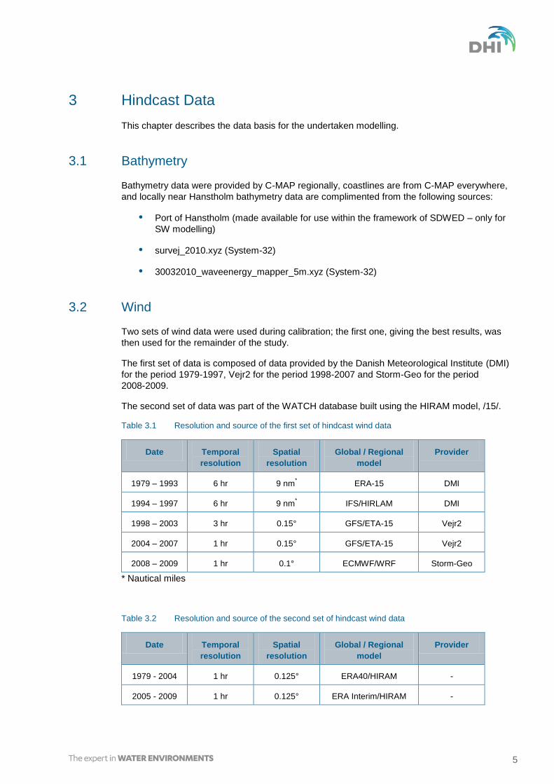
3.2 Wind
Two sets of wind data were used during calibration; the first one, giving the best results, was
then used for the remainder of the study.
The first set of data is composed of data provided by the Danish Meteorological Institute (DMI)
for the period 1979-1997, Vejr2 for the period 1998-2007 and Storm-Geo for the period
2008-2009.
The second set of data was part of the WATCH database built using the HIRAM model, /15/.
Table 3.1 Resolution and source of the first set of hindcast wind data
Date Temporal
resolution
Spatial
resolution
Global / Regional
model
Provider
1979 – 1993 6 hr 9 nm* ERA-15 DMI
1994 – 1997 6 hr 9 nm* IFS/HIRLAM DMI
1998 – 2003 3 hr 0.15° GFS/ETA-15 Vejr2
2004 – 2007 1 hr 0.15° GFS/ETA-15 Vejr2
2008 – 2009 1 hr 0.1° ECMWF/WRF Storm-Geo
* Nautical miles
Table 3.2 Resolution and source of the second set of hindcast wind data
Date Temporal
resolution
Spatial
resolution
Global / Regional
model
Provider
1979 - 2004 1 hr 0.125° ERA40/HIRAM -
2005 - 2009 1 hr 0.125° ERA Interim/HIRAM -
6 11804965 SDWED Long-term Wave Prediction D1.1/jts/mgo/ybr/pot – 09Apr13
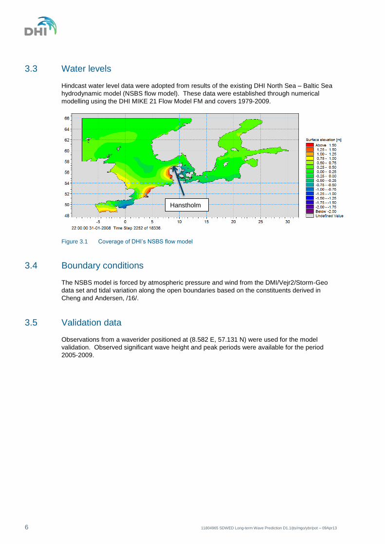
3.3 Water levels
Hindcast water level data were adopted from results of the existing DHI North Sea – Baltic Sea
hydrodynamic model (NSBS flow model). These data were established through numerical
modelling using the DHI MIKE 21 Flow Model FM and covers 1979-2009.
Figure 3.1 Coverage of DHI’s NSBS flow model
3.4 Boundary conditions
The NSBS model is forced by atmospheric pressure and wind from the DMI/Vejr2/Storm-Geo
data set and tidal variation along the open boundaries based on the constituents derived in
Cheng and Andersen, /16/.
3.5 Validation data
Observations from a waverider positioned at (8.582 E, 57.131 N) were used for the model
validation. Observed significant wave height and peak periods were available for the period
2005-2009.
Hanstholm
7
4 Spectral Wave Model Set-up
Hindcast wave data were established using MIKE 21 Spectral Waves (WS).
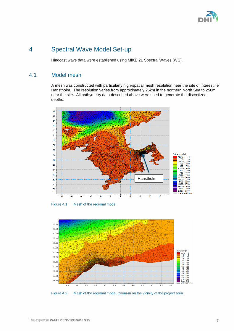
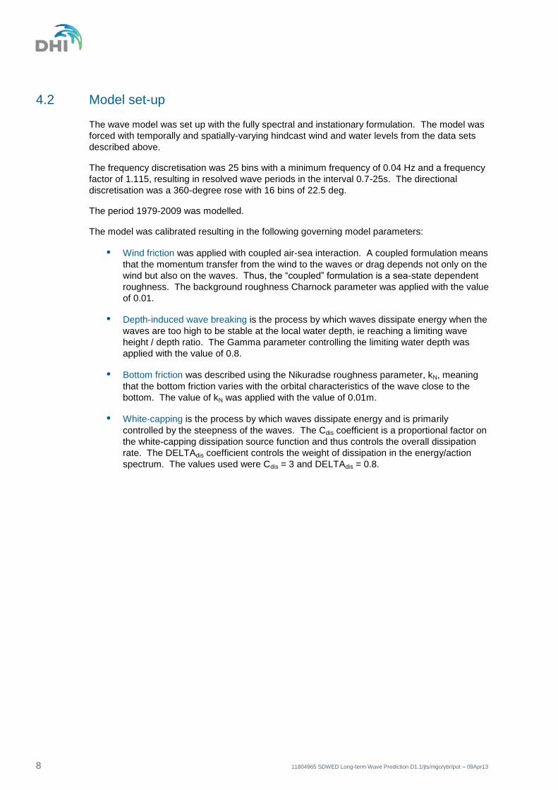
4.1 Model mesh
A mesh was constructed with particularly high-spatial mesh resolution near the site of interest, ie
Hanstholm. The resolution varies from approximately 25km in the northern North Sea to 250m
near the site. All bathymetry data described above were used to generate the discretized
depths.
Figure 4.1 Mesh of the regional model
Figure 4.2 Mesh of the regional model, zoom-in on the vicinity of the project area
Hanstholm
8 11804965 SDWED Long-term Wave Prediction D1.1/jts/mgo/ybr/pot – 09Apr13
4.2 Model set-up
The wave model was set up with the fully spectral and instationary formulation. The model was
forced with temporally and spatially-varying hindcast wind and water levels from the data sets
described above.
The frequency discretisation was 25 bins with a minimum frequency of 0.04 Hz and a frequency
factor of 1.115, resulting in resolved wave periods in the interval 0.7-25s. The directional
discretisation was a 360-degree rose with 16 bins of 22.5 deg.
The period 1979-2009 was modelled.
The model was calibrated resulting in the following governing model parameters:
Wind friction was applied with coupled air-sea interaction. A coupled formulation means
that the momentum transfer from the wind to the waves or drag depends not only on the
wind but also on the waves. Thus, the “coupled” formulation is a sea-state dependent
roughness. The background roughness Charnock parameter was applied with the value
of 0.01.
Depth-induced wave breaking is the process by which waves dissipate energy when the
waves are too high to be stable at the local water depth, ie reaching a limiting wave
height / depth ratio. The Gamma parameter controlling the limiting water depth was
applied with the value of 0.8.
Bottom friction was described using the Nikuradse roughness parameter, kN, meaning
that the bottom friction varies with the orbital characteristics of the wave close to the
bottom. The value of kN was applied with the value of 0.01m.
White-capping is the process by which waves dissipate energy and is primarily
controlled by the steepness of the waves. The Cdis coefficient is a proportional factor on
the white-capping dissipation source function and thus controls the overall dissipation
rate. The DELTAdis coefficient controls the weight of dissipation in the energy/action
spectrum. The values used were Cdis = 3 and DELTAdis = 0.8.
9
5 Calibration and Validation Results
The calibration included the investigation of the following parameters and input data:
Bottom friction: roughness coefficient kN
White-capping: dissipation coefficients Cdis and DELTAdis
Air-sea drag: Charnock parameter
Input data: selection of the best wind data set
Input data: influence of open boundaries
Based on a multi objective analysis of both the predicted and observed significant wave height,
zero-crossing and peak period distributions, the above wind data and parameters were selected
by a trial and error calibration process. The year 2007 was primarily used for the calibration of
the wave model.
The key parameters considered in the calibration were: the scatter index, bias and the peak
ratio.
See Appendix A for details on the statistical analysis methods used.
The significant wave height performance of the calibrated model over the calibration period can
be seen in Figure 5.1.

10 11804965 SDWED Long-term Wave Prediction D1.1/jts/mgo/ybr/pot – 09Apr13
Figure 5.1 Significant wave height at Hanstholm, model and observations (final parameters)
11
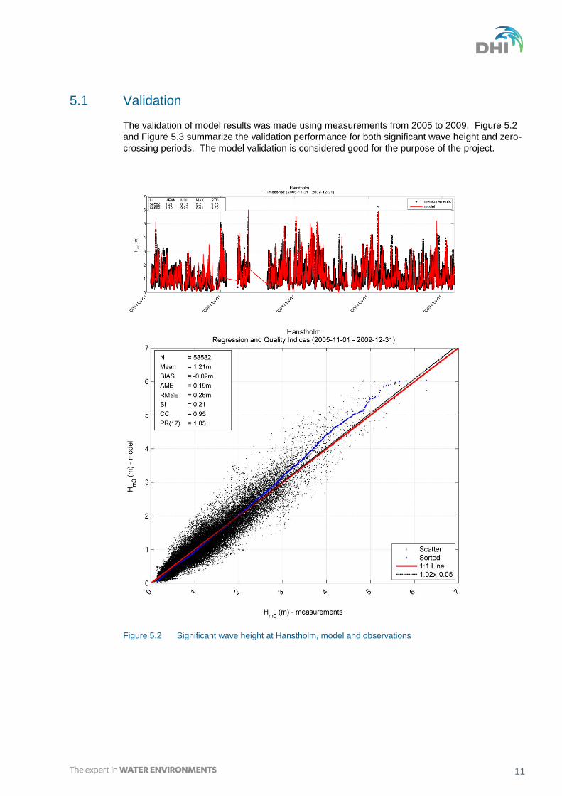
5.1 Validation
The validation of model results was made using measurements from 2005 to 2009. Figure 5.2
and Figure 5.3 summarize the validation performance for both significant wave height and zero-
crossing periods. The model validation is considered good for the purpose of the project.
Figure 5.2 Significant wave height at Hanstholm, model and observations

12 11804965 SDWED Long-term Wave Prediction D1.1/jts/mgo/ybr/pot – 09Apr13
Figure 5.3 Zero-crossing wave period, model and observations

13
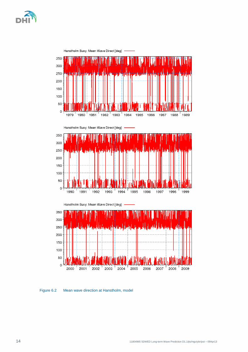
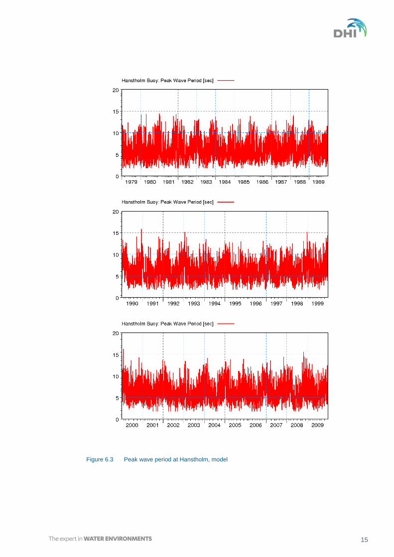
6 Spectral Data, Wave Power Maps
In order to provide spectral hindcast data for five production sea states and two extreme events,
a selection of appropriate periods has been made, through a time series visual analysis. Figure
6.1 - Figure 6.3 show 30-year time series of wave power, mean wave direction and peak wave
period at the monitoring position.
Figure 6.1 Wave power at Hanstholm, model
14 11804965 SDWED Long-term Wave Prediction D1.1/jts/mgo/ybr/pot – 09Apr13
Figure 6.2 Mean wave direction at Hanstholm, model
15
Figure 6.3 Peak wave period at Hanstholm, model
16 11804965 SDWED Long-term Wave Prediction D1.1/jts/mgo/ybr/pot – 09Apr13
6.1 Spectra
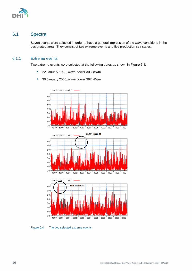
Seven events were selected in order to have a general impression of the wave conditions in the
designated area. They consist of two extreme events and five production sea states.
6.1.1 Extreme events
Two extreme events were selected at the following dates as shown in Figure 6.4:
22 January 1993, wave power 308 kW/m
30 January 2000, wave power 397 kW/m
Figure 6.4 The two selected extreme events
17
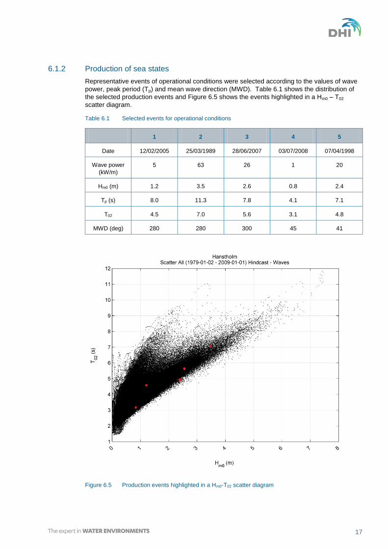
6.1.2 Production of sea states
Representative events of operational conditions were selected according to the values of wave
power, peak period (Tp) and mean wave direction (MWD). Table 6.1 shows the distribution of
the selected production events and Figure 6.5 shows the events highlighted in a Hm0 – T02
scatter diagram.
Table 6.1 Selected events for operational conditions
1 2 3 4 5
Date 12/02/2005 25/03/1989 28/06/2007 03/07/2008 07/04/1998
Wave power
(kW/m)
5 63 26 1 20
Hm0 (m) 1.2 3.5 2.6 0.8 2.4
Tp (s) 8.0 11.3 7.8 4.1 7.1
T02 4.5 7.0 5.6 3.1 4.8
MWD (deg) 280 280 300 45 41
Figure 6.5 Production events highlighted in a Hm0-T02 scatter diagram
18 11804965 SDWED Long-term Wave Prediction D1.1/jts/mgo/ybr/pot – 09Apr13
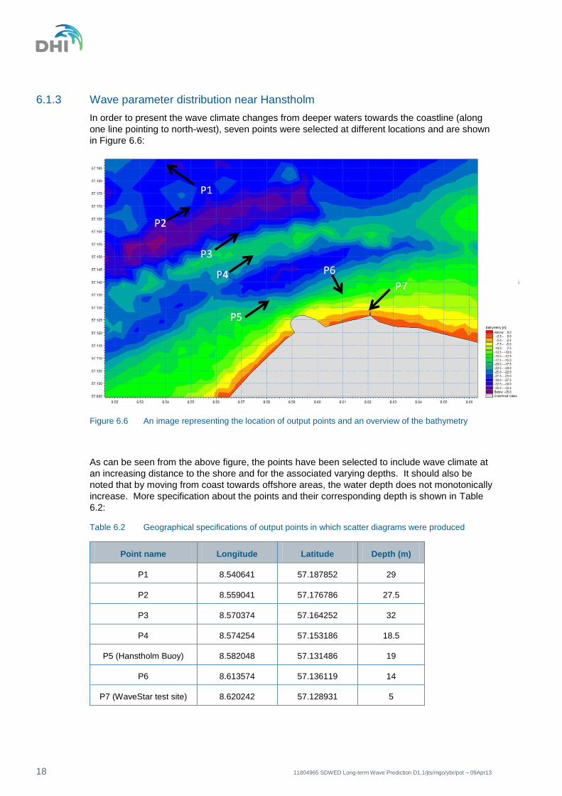
6.1.3 Wave parameter distribution near Hanstholm
In order to present the wave climate changes from deeper waters towards the coastline (along
one line pointing to north-west), seven points were selected at different locations and are shown
in Figure 6.6:
Figure 6.6 An image representing the location of output points and an overview of the bathymetry
As can be seen from the above figure, the points have been selected to include wave climate at
an increasing distance to the shore and for the associated varying depths. It should also be
noted that by moving from coast towards offshore areas, the water depth does not monotonically
increase. More specification about the points and their corresponding depth is shown in Table
6.2:
Table 6.2 Geographical specifications of output points in which scatter diagrams were produced
Point name Longitude Latitude Depth (m)
P1 8.540641 57.187852 29
P2 8.559041 57.176786 27.5
P3 8.570374 57.164252 32
P4 8.574254 57.153186 18.5
P5 (Hanstholm Buoy) 8.582048 57.131486 19
P6 8.613574 57.136119 14
P7 (WaveStar test site) 8.620242 57.128931 5
19
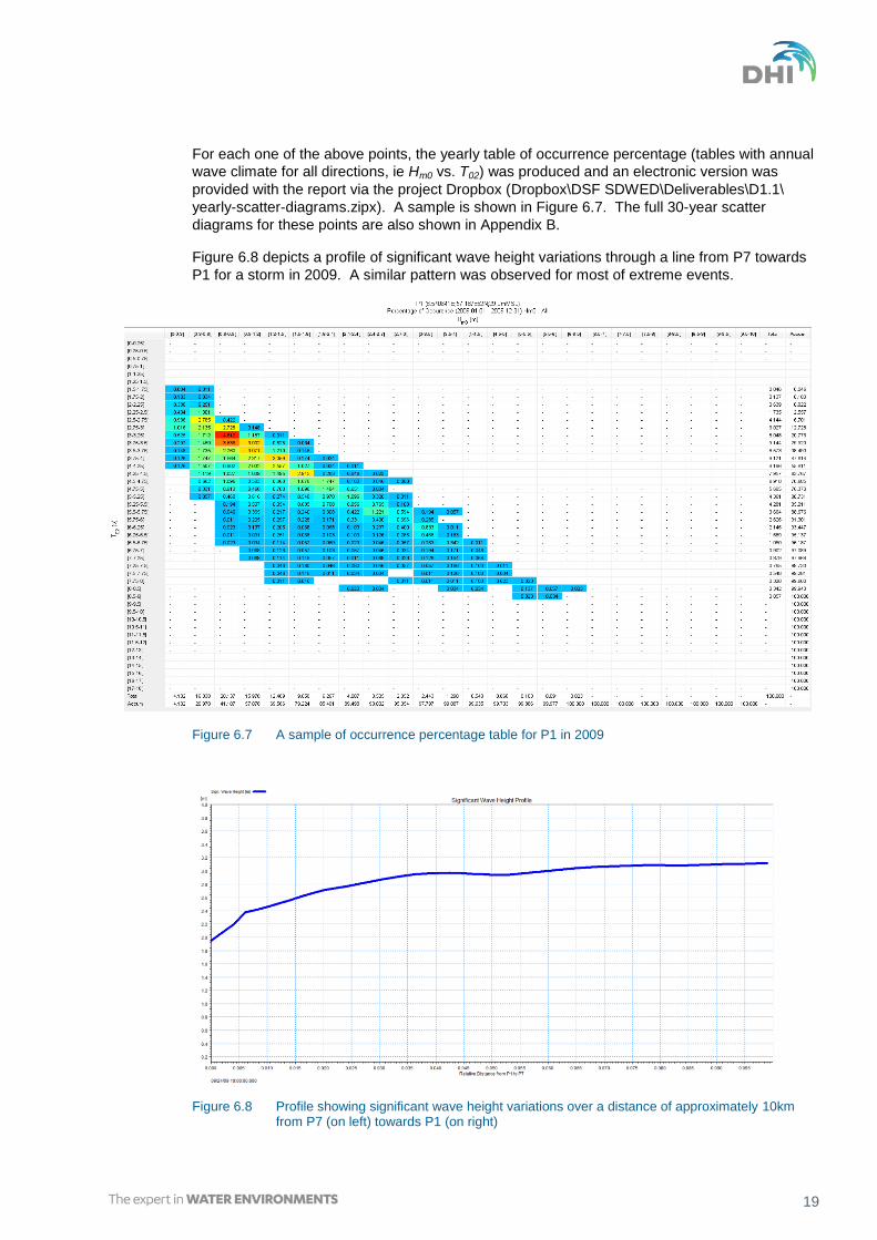
For each one of the above points, the yearly table of occurrence percentage (tables with annual
wave climate for all directions, ie Hm0 vs. T02) was produced and an electronic version was
provided with the report via the project Dropbox (Dropbox\DSF SDWED\Deliverables\D1.1\
yearly-scatter-diagrams.zipx). A sample is shown in Figure 6.7. The full 30-year scatter
diagrams for these points are also shown in Appendix B.
Figure 6.8 depicts a profile of significant wave height variations through a line from P7 towards
P1 for a storm in 2009. A similar pattern was observed for most of extreme events.
Figure 6.7 A sample of occurrence percentage table for P1 in 2009
Figure 6.8 Profile showing significant wave height variations over a distance of approximately 10km from P7 (on left) towards P1 (on right)
20 11804965 SDWED Long-term Wave Prediction D1.1/jts/mgo/ybr/pot – 09Apr13
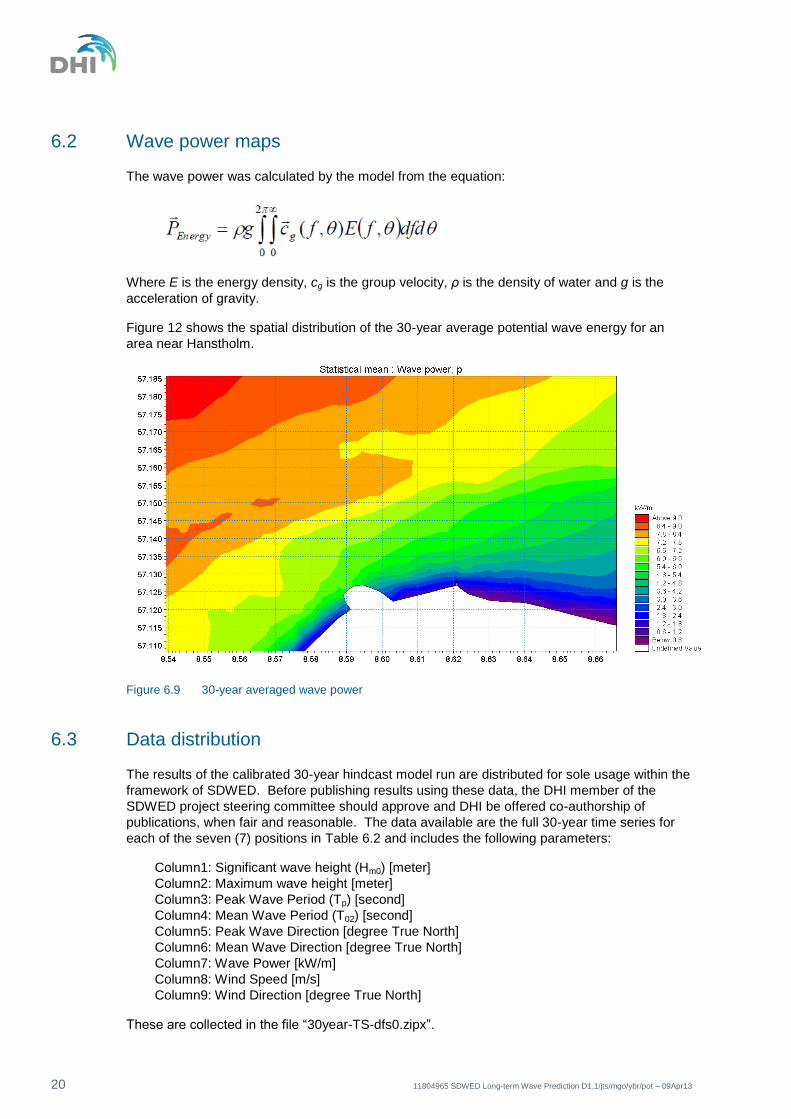
6.2 Wave power maps
The wave power was calculated by the model from the equation:
Where E is the energy density, cg is the group velocity, ρ is the density of water and g is the
acceleration of gravity.
Figure 12 shows the spatial distribution of the 30-year average potential wave energy for an
area near Hanstholm.
Figure 6.9 30-year averaged wave power
6.3 Data distribution
The results of the calibrated 30-year hindcast model run are distributed for sole usage within the
framework of SDWED. Before publishing results using these data, the DHI member of the
SDWED project steering committee should approve and DHI be offered co-authorship of
publications, when fair and reasonable. The data available are the full 30-year time series for
each of the seven (7) positions in Table 6.2 and includes the following parameters:
Column1: Significant wave height (Hm0) [meter]
Column2: Maximum wave height [meter]
Column3: Peak Wave Period (Tp) [second]
Column4: Mean Wave Period (T02) [second]
Column5: Peak Wave Direction [degree True North]
Column6: Mean Wave Direction [degree True North]
Column7: Wave Power [kW/m]
Column8: Wind Speed [m/s]
Column9: Wind Direction [degree True North]
These are collected in the file “30year-TS-dfs0.zipx”.

21
A MATLAB program is further supplied for reading the dfs0 time series. To use this program,
the instructions described via the link for download of DHI MATLAB Toolbox should be followed:
http://mikebydhi.com/Download/DocumentsAndTools/Tools/DHIMatLabToolbox.aspx.
Further, full spectral and directional time series are provided for positions 5 and 7. These data
are distributed by the project manager upon request due to the large size of the file. The data
file is named “Stations-DF-Spectra.dfs2”.

22 11804965 SDWED Long-term Wave Prediction D1.1/jts/mgo/ybr/pot – 09Apr13
23
7 Summary
This report has summarized the derivation of reliable long-term wave conditions near Hanstholm
and presented the spatio-temporal distribution of the waves and their associated energy. The
intention is that the distributed data sets are used as input to other WP1 tasks, WP4 and WP5.

24 11804965 SDWED Long-term Wave Prediction D1.1/jts/mgo/ybr/pot – 09Apr13
25
8 References
/1/ MIKE 21 SW scientific documentation
/2/ Komen, G.J., K. Hasselmann and S. Hasselmann, (1984) 'On the existence of a fully
developed windsea spectrum.' Journal of Physical Oceanography 14, 1271-1285.
/3/ Young, I.R., 1999: Wind generated ocean waves, Eds. R. Bhattacharyya and M.E.
McCormick, Ocean Engineering Series, Elsevier, Amsterdam, 288 pp.
/4/ Janssen, P.A.E.M., 1989: Wave induced stress and the drag of air flow over sea waves,
J. Phys. Oceanogr., 19, 745-754.
/5/ Janssen, P.A.E.M., Lionello, P. and Zambresky, L., 1989: On the interaction of wind and
waves, Phil. Trans. R Soc. Lond., A 329, 289-301.
/6/ Janssen, P.A.E.M (1991) ‘Quasi-linear Theory of Wind-Wave Generation Applied to Wave
Forecasting’ Journal of Physical Oceanography 21, 1631-1642.
/7/ Hasselmann, K., 1962: On the non-linear transfer in a gravity wave spectrum, part 1.
General theory, J. Fluid Mech., 12, 481-500.
/8/ Hasselmann, S.K., Hasselmann, J., Allender, H. and Barnett, T. P. (1985) 'Computations
and parameterizations of the nonlinear transfer in a gravity-wave spectrum. Part I A new
method for efficient computations of the exact nonlinear transfer integral.' Journal of
Physical Oceanography 15, 1369-1377.
/9/ Hasselmann, S.K., Hasselmann, J., Allender, H. and Barnett, T. P. (1985) 'Computations
and parameterizations of the nonlinear transfer in a gravity-wave spectrum. Part II.
Parameterizations of the nonlinear transfer for application in wave models.' Journal of
Physical Oceanography 15, 1378-1391.
/10/ Eldeberky, Y. and J.A. Battjes, 1995: Parameterization of triad interactions in wave
energy models, Proc. Coastal Dynamics Conf. ’95, Gdansk, Poland, 140-148
/11/ Eldeberky, Y. and J. A. Battjes, 1996: Spectral modelling of wave breaking. J. Geophys.
Res., 101, 1253-1264.
/12/ Johnson, Hakeem K., Henrik Kofoed-Hansen, 2000: Influence of Bottom Friction on Sea
Surface Roughness and Its Impact on Shallow Water Wind Wave Modeling. J. Phys.
Oceanogr., 30, 1743–1756.
/13/ Battjes J. A. and J. P. F. M. Janssen, 1978: Energy loss and set-up due to breaking of
random waves. In Proc. of the 16th Int. Conf. Coastal Engineering, 569-587, Hamburg
Germany.
/14/ Holthuijsen L.H., Herman A. and Booij N., 2003: Phase-decoupled refraction-difraction for
spectral wave models, Coastal Engineering, 49, 291-305.
/15/ FP6 project, Ensembles, http://ensembles-eu.metoffice.com/
/16/ Yongcun Cheng, Ole Baltazar Andersen, (2010). Improvement in global ocean tide model
in shallow water regions. Poster, SV.1-68 45, OSTST, Lisbon, Oct.18-22.

26 11804965 SDWED Long-term Wave Prediction D1.1/jts/mgo/ybr/pot – 09Apr13

APPENDICES

11804965 SDWED Long-term Wave Prediction D1.1/jts/mgo/ybr/pot – 09Apr13

APPENDIX A
General Description of the QI

11804965 SDWED Long-term Wave Prediction D1.1/jts/mgo/ybr/pot – 09Apr13
A-1
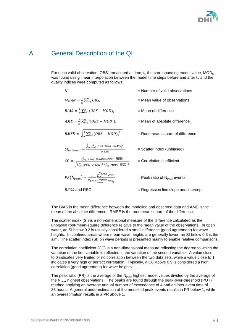
A General Description of the QI
For each valid observation, OBSi, measured at time, ti, the corresponding model value, MODi,
was found using linear interpolation between the model time steps before and after ti, and the
quality indices were computed as follows:
= Number of valid observations
∑
= Mean value of observations
∑
= Mean of difference
∑ | |
= Mean of absolute difference
√
∑
= Root mean square of difference
√
∑
= Scatter index (unbiased)
∑
√∑ ∑
= Correlation coefficient
( )
∑
∑
= Peak ratio of Npeak events
and REGI = Regression line slope and intercept
The BIAS is the mean difference between the modelled and observed data and AME is the
mean of the absolute difference. RMSE is the root mean square of the difference.
The scatter index (SI) is a non-dimensional measure of the difference calculated as the
unbiased root-mean-square difference relative to the mean value of the observations. In open
water, an SI below 0.2 is usually considered a small difference (good agreement) for wave
heights. In confined areas where mean wave heights are generally lower, an SI below 0.3 is the
aim. The scatter index (SI) on wave periods is presented mainly to enable relative comparisons.
The correlation coefficient (CC) is a non-dimensional measure reflecting the degree to which the
variation of the first variable is reflected in the variation of the second variable. A value close
to 0 indicates very limited or no correlation between the two data sets, while a value close to 1
indicates a very high or perfect correlation. Typically, a CC above 0.9 is considered a high
correlation (good agreement) for wave heights.
The peak ratio (PR) is the average of the Npeak highest model values divided by the average of
the Npeak highest observations. The peaks are found through the peak-over-threshold (POT)
method applying an average annual number of exceedance of 4 and an inter event time of
36 hours. A general underestimation of the modelled peak events results in PR below 1, while
an overestimation results in a PR above 1.
A-2 11804965 SDWED Long-term Wave Prediction D1.1/jts/mgo/ybr/pot – 09Apr13
The regression line slope and intercept (REGS and REGI) are found from a linear fit to the data
points in a least square sense. A regression line slope different from 1 may indicate a trend in
the difference.
In the scatter comparison figures, a blue dotted line with the legend “Sorted” is included. It
consists of sorted measurement data and model data. The data are sorted without respect to
each other from the lowest value to the highest (for example: the highest measured value is
presented against the highest modelled value even though they may not occur at the same
time). This removes time dependency and represents a statistical distribution between
measured and modelled values. For equal distribution of data values, the blue line will follow
the 1:1 line. If the data values are not evenly distributed, the blue line will be shifted away from
the 1:1 line towards the variables with the relatively higher values.
The quality indices should be considered averaged measures for the entire data set and may
not be representative of the quality during rare events.

APPENDIX B
The Full 30-year Scatter Diagrams for Points P1 to P7

11804965 SDWED Long-term Wave Prediction D1.1/jts/mgo/ybr/pot – 09Apr13
B-1
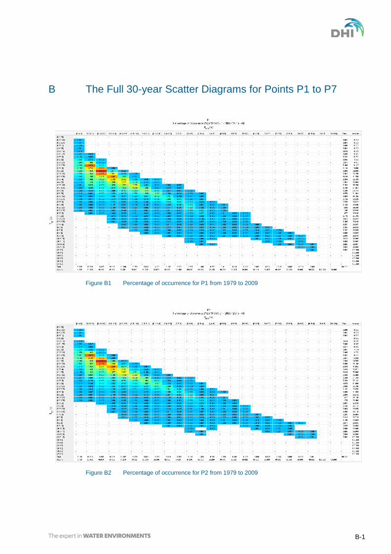
B The Full 30-year Scatter Diagrams for Points P1 to P7
Figure B1 Percentage of occurrence for P1 from 1979 to 2009
Figure B2 Percentage of occurrence for P2 from 1979 to 2009
B-2 11804965 SDWED Long-term Wave Prediction D1.1/jts/mgo/ybr/pot – 09Apr13
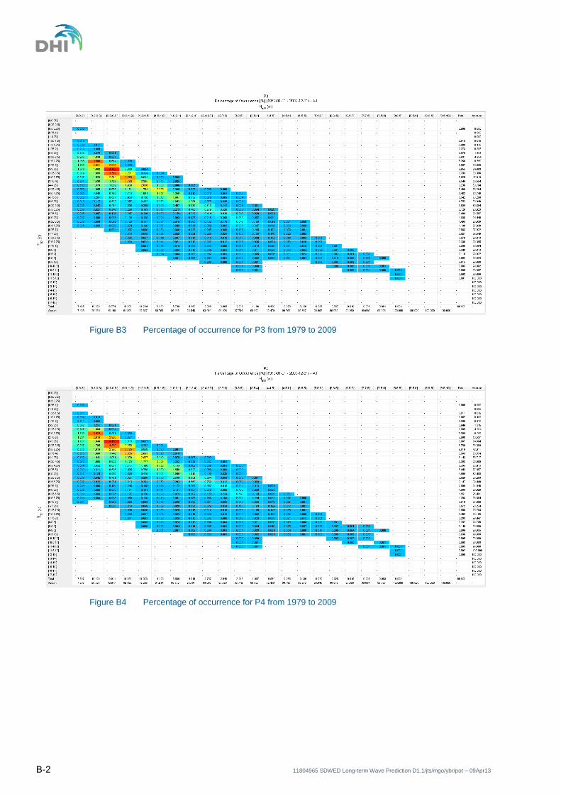
Figure B3 Percentage of occurrence for P3 from 1979 to 2009
Figure B4 Percentage of occurrence for P4 from 1979 to 2009
B-3
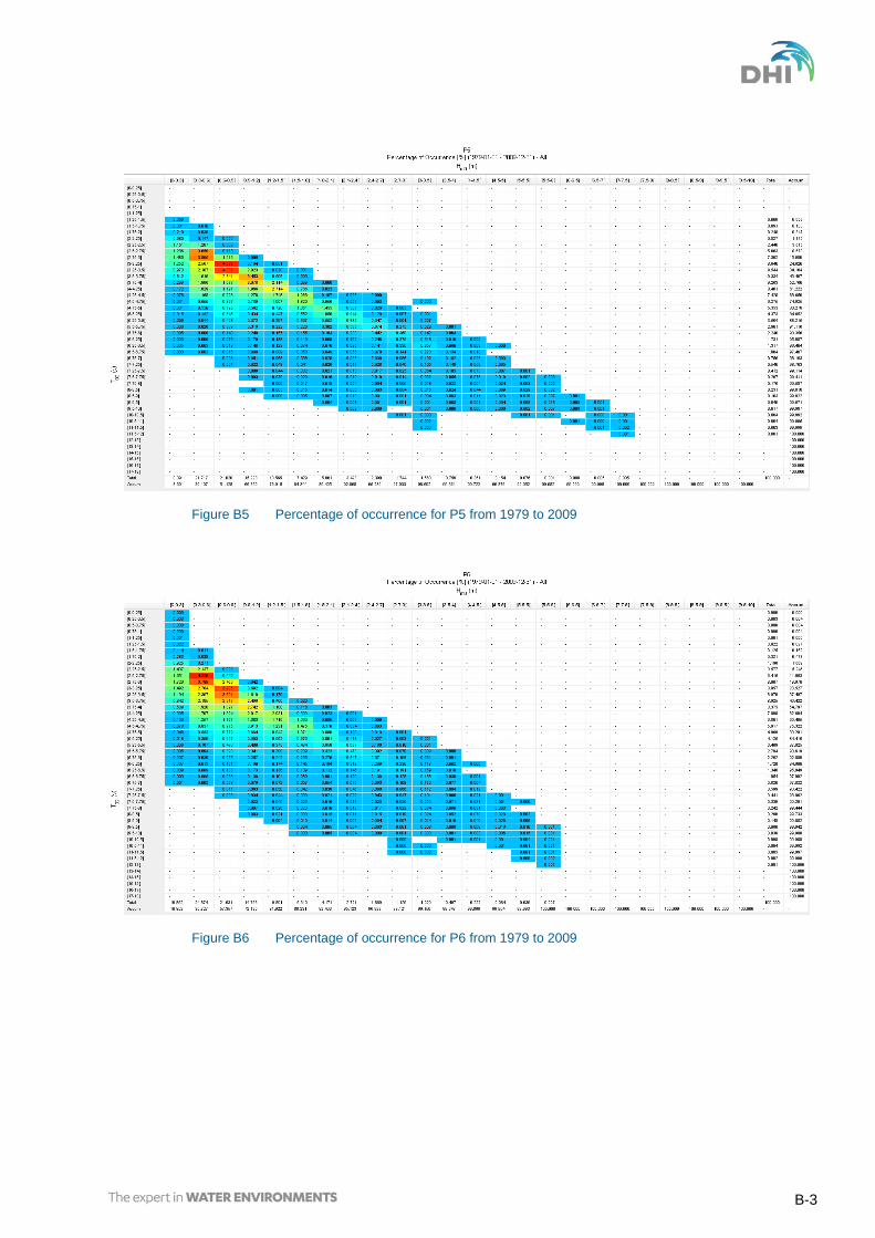
Figure B5 Percentage of occurrence for P5 from 1979 to 2009
Figure B6 Percentage of occurrence for P6 from 1979 to 2009
B-4 11804965 SDWED Long-term Wave Prediction D1.1/jts/mgo/ybr/pot – 09Apr13
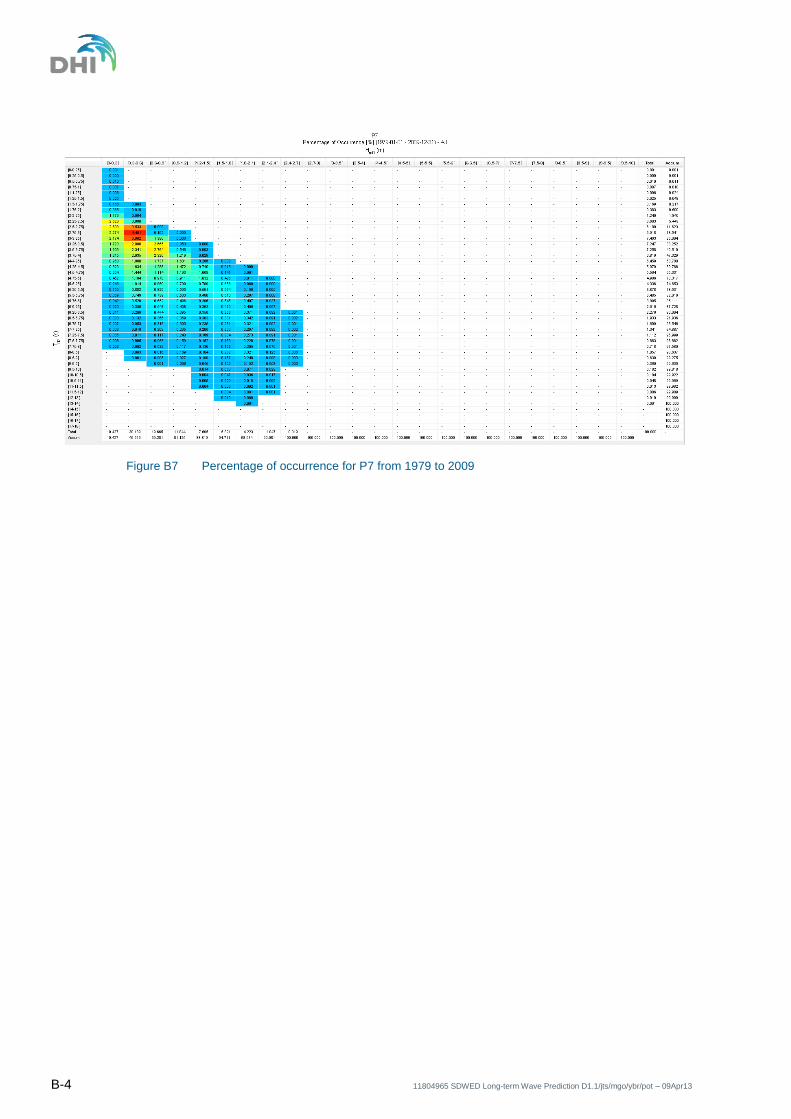
Figure B7 Percentage of occurrence for P7 from 1979 to 2009