Embed Size (px)
Citation preview
STRUCTURAL DAMAGE CLASSIFICATION COMPARISON USING
SUPPORT VECTOR MACHINE AND BAYESIAN MODEL SELECTION
Zhu Mao1, Michael Todd1
1 University of California at San Diego, 9500 Gilman Dr, MC0085, La Jolla, CA, USA 92093-0085
ABSTRACT
Since all damage identification strategies inevitably involve uncertainties from various
sources, a higher level of characterization is necessary to facilitate decision-making in
a statistically confident sense. Machine learning plays an important role in the
decision-making process of damage detection, classification, and prognosis, which
employs training data (or a validated model) and extracts useful information from the
high-dimensional observations. This paper classifies the type of damage via support
vector machine (SVM) in a supervised learning fashion, and selects the most plausible
model for data interpretation. Therefore the separation of damage type and failure
trajectory is transformed into a group classification process, under the influence of
uncertainty. Given data observation, SVM is obtained under a training process, which
characterizes the best classification boundaries for any future feature set. A rotary
machine test-bed is employed, and vibration-based damage features are evaluated to
demonstrate the proposed classification process.
KEYWORDS : damage classification, machine learning,support vector machine,
bearing failure.
1 INSTRUCTION
As the technology of structural damage detection and health monitoring is getting more and more
mature, lots of considerations have been addressed in dealing with the uncertainties involved in
making damage diagnosis/prognosis decisions. To make better decisions under uncertain scenarios
such as noisy measurements and operational variability, quantifying the uncertainty will enhance
the overall performance, and as a result, a quantified confidence in the decision will be available [1-
3]. In our previous research, probabilistic uncertainty quantification (UQ) models of frequency
response function (FRF) estimations are established, and the distributions of estimations from
different algorithms are fully characterized by the analytically derived probability density functions
[4, 5]. Bayesian statistics fuse collected evidence to update prior confidence and are powerful for
making decision especially when there is ambiguity caused by all sorts of uncertainty. For damage
classification applications, a Bayesian framework can be used to select the most plausible model to
characterize the data observations and classify the structural condition with respect to maximum
posterior probability [6].
Besides the uncertainty involved in damage detection and classification processes, extracting
sensitive and specific features from large volume of data set is another burden. Oftentimes, there is
great “fuzziness” and redundancy in the raw data coupled to the aforementioned uncertainty, and
this fundamentally causes the damage detection and classification processes to become more
complicated. Machine learning technologies have been employed widely in data processing and
feature extraction, among which support vector machines (SVM) are particularly powerful for
solving classification problems. This paper adopts an SVM to classify damage cases of the
Machinery Fault Simulator (MFS) from SpectraQuest, Inc., where damages on the outer race and
7th European Workshop on Structural Health Monitoring
July 8-11, 2014. La Cité, Nantes, France
Copyright © Inria (2014) 1973
Mor
e In
fo a
t Ope
n A
cces
s D
atab
ase
ww
w.n
dt.n
et/?
id=
1724
7
balls of bearings are differentiated from undamaged baseline. In this work, features are selected
based on FRF magnitude and phase, and rate of correct classification is defined as comparison
metric for different case studies.
A brief overview of FRF and the estimations on the test-bed will be given in section-2, and
SVM implementation on the data acquired from the test-bed, with a parametric study, is available in
section-3. In the end, a summary of the result is given in section-4.
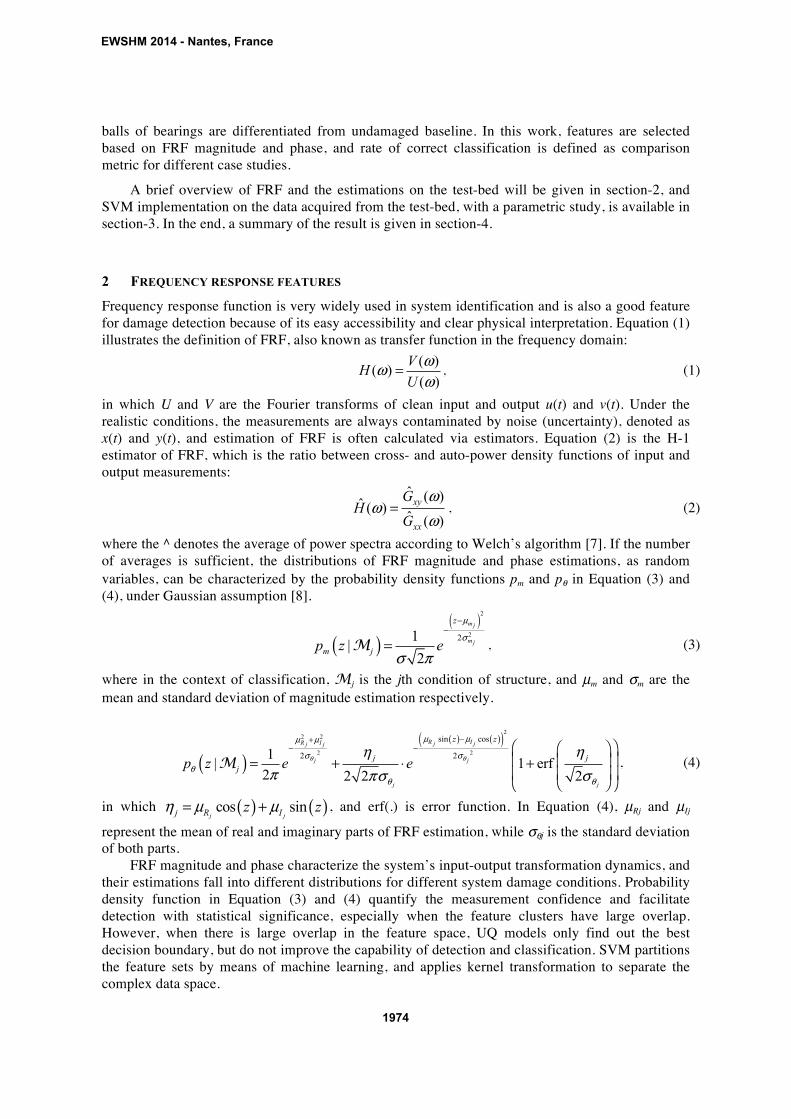
2 FREQUENCY RESPONSE FEATURES
Frequency response function is very widely used in system identification and is also a good feature
for damage detection because of its easy accessibility and clear physical interpretation. Equation (1)
illustrates the definition of FRF, also known as transfer function in the frequency domain:
( )
( )( )
VH
U
ωω
ω= , (1)
in which U and V are the Fourier transforms of clean input and output u(t) and v(t). Under the
realistic conditions, the measurements are always contaminated by noise (uncertainty), denoted as
x(t) and y(t), and estimation of FRF is often calculated via estimators. Equation (2) is the H-1
estimator of FRF, which is the ratio between cross- and auto-power density functions of input and
output measurements:
ˆ ( )
ˆ ( )ˆ ( )
xy
xx
GH
G
ωω
ω= , (2)
where the ^ denotes the average of power spectra according to Welch’s algorithm [7]. If the number
of averages is sufficient, the distributions of FRF magnitude and phase estimations, as random
variables, can be characterized by the probability density functions pm and pθ in Equation (3) and
(4), under Gaussian assumption [8].
( )
( )2
221|
2
mj
mj
z
m jp z e
µ
σ
σ π
−
−
=M , (3)
where in the context of classification, Mj is the jth condition of structure, and µm and σm are the
mean and standard deviation of magnitude estimation respectively.
( )
( ) ( )( )2
2 2
2 2
sin cos
2 21| 1 erf
2 2 2 2
R IR I j jj j
j j
j j
z z
j j
jp z e e
θ θ
µ µµ µ
σ σθ
θ θ
η ηπ πσ σ
−+− − ⎛ ⎞⎛ ⎞
⎜ ⎟⎜ ⎟= + ⋅ +⎜ ⎟⎜ ⎟⎝ ⎠⎝ ⎠
M , (4)
in which ( ) ( )cos sinj jj R I
z zη µ µ= + , and erf(.) is error function. In Equation (4), µRj and µIj
represent the mean of real and imaginary parts of FRF estimation, while σθj is the standard deviation
of both parts.
FRF magnitude and phase characterize the system’s input-output transformation dynamics, and
their estimations fall into different distributions for different system damage conditions. Probability
density function in Equation (3) and (4) quantify the measurement confidence and facilitate
detection with statistical significance, especially when the feature clusters have large overlap.
However, when there is large overlap in the feature space, UQ models only find out the best
decision boundary, but do not improve the capability of detection and classification. SVM partitions
the feature sets by means of machine learning, and applies kernel transformation to separate the
complex data space.
EWSHM 2014 - Nantes, France
1974
3 SVM AND IMPLEMENTATION
3.1 SVM and kernelization
SVM employs training data to form a hyperplane as the decision boundary, in order to discriminate
different sets of data, and all the data points determining the hyperplane are called support vectors.
Equation (5) describes the decision maker h(*), which maps feature vector x into a binary space:
( )( )
( )
0 if g 0h
1 if g 0
⎧ >⎪= ⎨
<⎪⎩
xx
x. (5)
The function g(*) is a hyperplane in the feature space:
( )gT
= +x w x b . (6)
When the data from the classification model are non-separable, slack variables are introduced
to solve a soft margin problem, but this may not always practical for highly overlapped/complicated
feature spaces. Kernel functions are employed if necessary, so that the feature dimension is
increased, and all clusters are being better distinguished in a higher dimensional state, as Equation
(7) shows:
( ) ( )* *
SV
h sign K ,i i i
i
y∈
⎡ ⎤= +⎢ ⎥
⎣ ⎦∑x α x x b , (7)
in which xi are all the support vectors, K(*,*) is the selected kernel function, α i is the Lagrange
multiplier for constrained optimization, and yi is the classification label of feature xi.
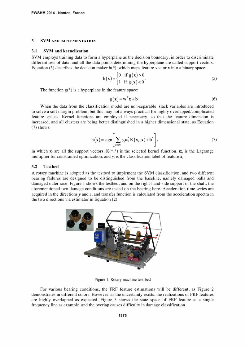
3.2 Testbed
A rotary machine is adopted as the testbed to implement the SVM classification, and two different
bearing failures are designed to be distinguished from the baseline, namely damaged balls and
damaged outer race. Figure 1 shows the testbed, and on the right-hand-side support of the shaft, the
aforementioned two damage conditions are tested on the bearing here. Acceleration time series are
acquired in the directions y and z, and transfer function is calculated from the acceleration spectra in
the two directions via estimator in Equation (2).
Figure 1: Rotary machine test-bed
For various bearing conditions, the FRF feature estimations will be different, as Figure 2
demonstrates in different colors. However, as the uncertainty exists, the realizations of FRF features
are highly overlapped as expected. Figure 3 shows the state space of FRF feature at a single
frequency line as example, and the overlap causes difficulty in damage classification.
x
y
z
EWSHM 2014 - Nantes, France
1975
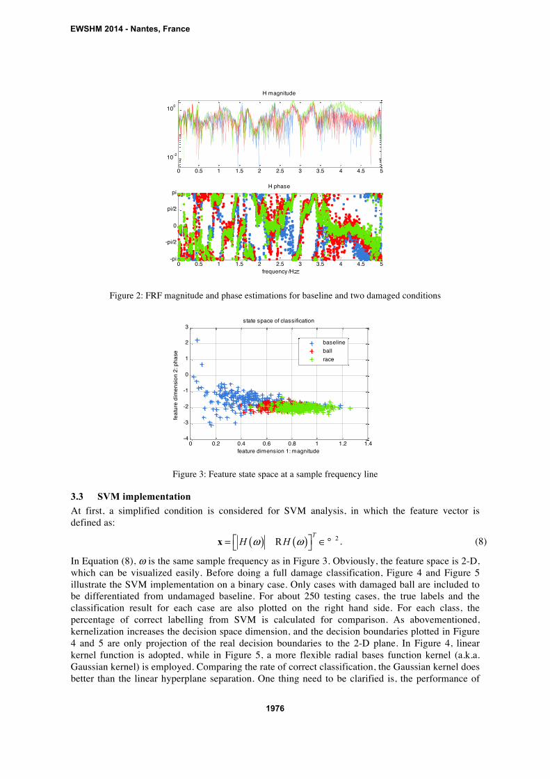
Figure 2: FRF magnitude and phase estimations for baseline and two damaged conditions
Figure 3: Feature state space at a sample frequency line
3.3 SVM implementation
At first, a simplified condition is considered for SVM analysis, in which the feature vector is
defined as:
( ) ( ) 2T
H Hω ω⎡ ⎤= ∈⎣ ⎦x R ° . (8)
In Equation (8), ω is the same sample frequency as in Figure 3. Obviously, the feature space is 2-D,
which can be visualized easily. Before doing a full damage classification, Figure 4 and Figure 5
illustrate the SVM implementation on a binary case. Only cases with damaged ball are included to
be differentiated from undamaged baseline. For about 250 testing cases, the true labels and the
classification result for each case are also plotted on the right hand side. For each class, the
percentage of correct labelling from SVM is calculated for comparison. As abovementioned,
kernelization increases the decision space dimension, and the decision boundaries plotted in Figure
4 and 5 are only projection of the real decision boundaries to the 2-D plane. In Figure 4, linear
kernel function is adopted, while in Figure 5, a more flexible radial bases function kernel (a.k.a.
Gaussian kernel) is employed. Comparing the rate of correct classification, the Gaussian kernel does
better than the linear hyperplane separation. One thing need to be clarified is, the performance of
0 0.5 1 1.5 2 2.5 3 3.5 4 4.5 5
10-2
100
H magnitude
0 0.5 1 1.5 2 2.5 3 3.5 4 4.5 5-pi
-pi/2
0
pi/2
piH phase
frequency /Hz
0 0.2 0.4 0.6 0.8 1 1.2 1.4-4
-3
-2
-1
0
1
2
3
feature dimension 1: magnitude
fea
ture
dim
en
sio
n 2
: p
ha
se
state space of classification
baseline
ball
race
EWSHM 2014 - Nantes, France
1976
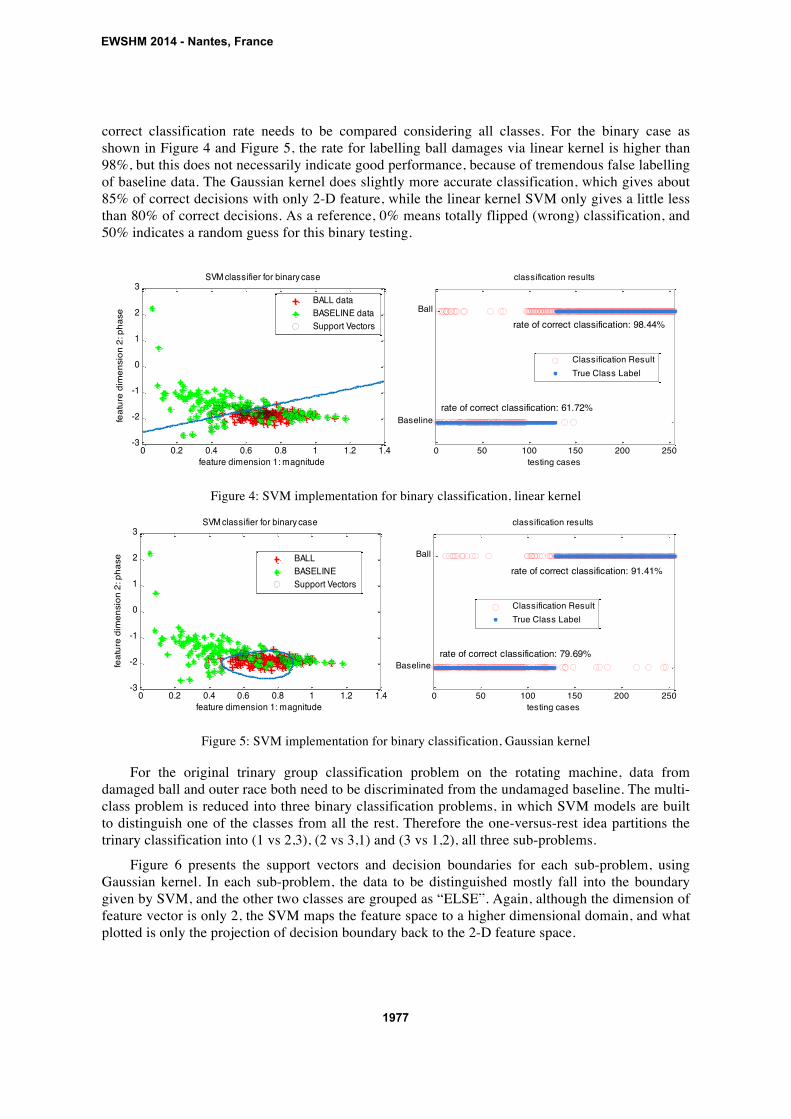
correct classification rate needs to be compared considering all classes. For the binary case as
shown in Figure 4 and Figure 5, the rate for labelling ball damages via linear kernel is higher than
98%, but this does not necessarily indicate good performance, because of tremendous false labelling
of baseline data. The Gaussian kernel does slightly more accurate classification, which gives about
85% of correct decisions with only 2-D feature, while the linear kernel SVM only gives a little less
than 80% of correct decisions. As a reference, 0% means totally flipped (wrong) classification, and
50% indicates a random guess for this binary testing.
Figure 4: SVM implementation for binary classification, linear kernel
Figure 5: SVM implementation for binary classification, Gaussian kernel
For the original trinary group classification problem on the rotating machine, data from
damaged ball and outer race both need to be discriminated from the undamaged baseline. The multi-
class problem is reduced into three binary classification problems, in which SVM models are built
to distinguish one of the classes from all the rest. Therefore the one-versus-rest idea partitions the
trinary classification into (1 vs 2,3), (2 vs 3,1) and (3 vs 1,2), all three sub-problems.
Figure 6 presents the support vectors and decision boundaries for each sub-problem, using
Gaussian kernel. In each sub-problem, the data to be distinguished mostly fall into the boundary
given by SVM, and the other two classes are grouped as “ELSE”. Again, although the dimension of
feature vector is only 2, the SVM maps the feature space to a higher dimensional domain, and what
plotted is only the projection of decision boundary back to the 2-D feature space.
0 0.2 0.4 0.6 0.8 1 1.2 1.4-3
-2
-1
0
1
2
3
feature dimension 1: magnitude
fea
ture
dim
en
sio
n 2
: p
ha
se
SVM classifier for binary case
BALL data
BASELINE data
Support Vectors
0 50 100 150 200 250
Baseline
Ball
testing cases
classification results
rate of correct classification: 61.72%
rate of correct classification: 98.44%
Classification Result
True Class Label
0 0.2 0.4 0.6 0.8 1 1.2 1.4-3
-2
-1
0
1
2
3
feature dimension 1: magnitude
fea
ture
dim
en
sio
n 2
: p
ha
se
SVM classifier for binary case
BALL
BASELINE
Support Vectors
0 50 100 150 200 250
Baseline
Ball
testing cases
classification results
rate of correct classification: 79.69%
rate of correct classification: 91.41%
Classification Result
True Class Label
EWSHM 2014 - Nantes, France
1977
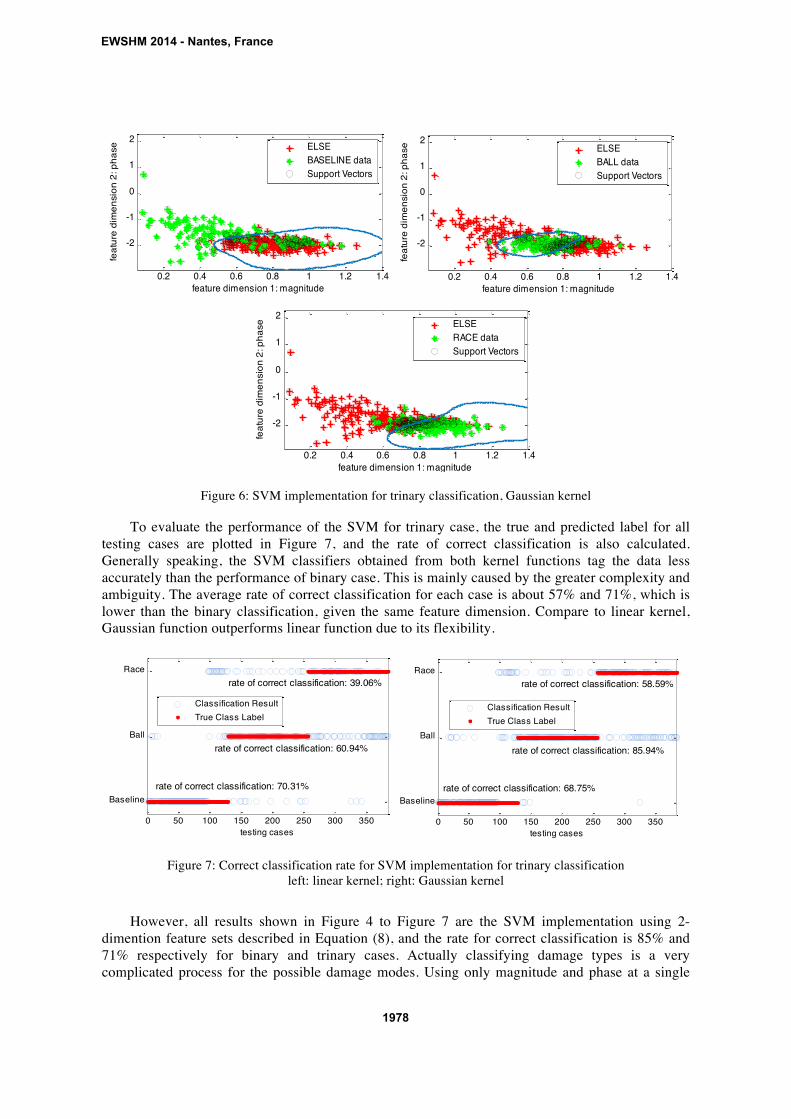
Figure 6: SVM implementation for trinary classification, Gaussian kernel
To evaluate the performance of the SVM for trinary case, the true and predicted label for all
testing cases are plotted in Figure 7, and the rate of correct classification is also calculated.
Generally speaking, the SVM classifiers obtained from both kernel functions tag the data less
accurately than the performance of binary case. This is mainly caused by the greater complexity and
ambiguity. The average rate of correct classification for each case is about 57% and 71%, which is
lower than the binary classification, given the same feature dimension. Compare to linear kernel,
Gaussian function outperforms linear function due to its flexibility.
Figure 7: Correct classification rate for SVM implementation for trinary classification
left: linear kernel; right: Gaussian kernel
However, all results shown in Figure 4 to Figure 7 are the SVM implementation using 2-
dimention feature sets described in Equation (8), and the rate for correct classification is 85% and
71% respectively for binary and trinary cases. Actually classifying damage types is a very
complicated process for the possible damage modes. Using only magnitude and phase at a single
0.2 0.4 0.6 0.8 1 1.2 1.4
-2
-1
0
1
2
feature dimension 1: magnitude
fea
ture
dim
en
sio
n 2
: p
ha
se
ELSE
BASELINE data
Support Vectors
0.2 0.4 0.6 0.8 1 1.2 1.4
-2
-1
0
1
2
feature dimension 1: magnitude
fea
ture
dim
en
sio
n 2
: p
ha
se
ELSE
BALL data
Support Vectors
0.2 0.4 0.6 0.8 1 1.2 1.4
-2
-1
0
1
2
feature dimension 1: magnitude
fea
ture
dim
en
sio
n 2
: p
ha
se
ELSE
RACE data
Support Vectors
0 50 100 150 200 250 300 350
Baseline
Ball
Race
testing cases
rate of correct classification: 70.31%
rate of correct classification: 60.94%
rate of correct classification: 39.06%
Classification Result
True Class Label
0 50 100 150 200 250 300 350
Baseline
Ball
Race
testing cases
rate of correct classification: 68.75%
rate of correct classification: 85.94%
rate of correct classification: 58.59%
Classification Result
True Class Label
EWSHM 2014 - Nantes, France
1978
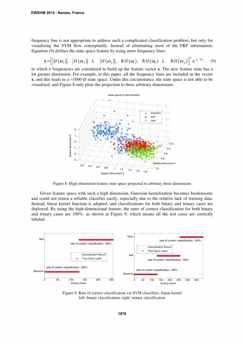
frequency line is not appropriate to address such a complicated classification problem, but only for
visualizing the SVM flow conceptually. Instead of eliminating most of the FRF information,
Equation (9) defines the state space feature by using more frequency lines:
( ) ( ) ( ) ( ) ( ) ( ) 2
1 2 1 2, , ,T
n
n nH H H H H Hω ω ω ω ω ω⎡ ⎤= ∈⎣ ⎦x L R R L R ° . (9)
in which n frequencies are considered to build up the feature vector x. The new feature state has a
lot greater dimension. For example, in this paper, all the frequency lines are included in the vector
x, and this leads to a ~1000-D state space. Under this circumstance, the state space is not able to be
visualized, and Figure 8 only plots the projection to three arbitrary dimensions.
Figure 8: High-dimension feature state space projected to arbitrary three dimensions
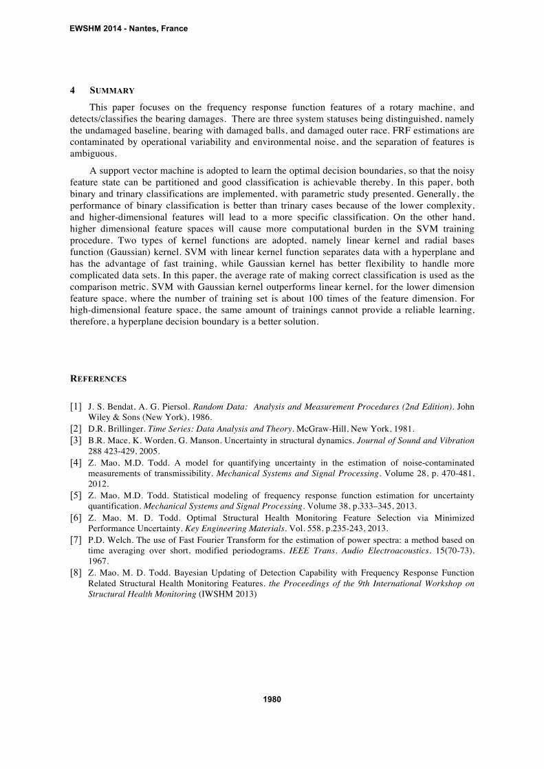
Given feature space with such a high dimension, Gaussian kernelization becomes burdensome
and could not return a reliable classifier easily, especially due to the relative lack of training data.
Instead, linear kernel function is adopted, and classifications for both binary and trinary cases are
deployed. By using the high-dimensional feature, the rates of correct classification for both binary
and trinary cases are 100%, as shown in Figure 9, which means all the test cases are correctly
labeled.
Figure 9: Rate of correct classification via SVM classifiers, linear kernel
left: binary classification; right: trinary classification
0.2
0.4
0.6
0.8
1
1.2
0.2 0.4 0.6 0.8 1 1.2 1.4 1.6 1.8
-3
-2
-1
0
1
2
feature dimension 1
feature dimension 2
state space of classification
fea
ture
dim
en
sio
n 3
baseline
ball
race
0 50 100 150 200 250
Baseline
Ball
testing cases
rate of correct classification: 100%
rate of correct classification: 100%
Classification Result
True Class Label
0 50 100 150 200 250 300 350
Baseline
Ball
Race
testing cases
rate of correct classification: 100%
rate of correct classification: 100%
rate of correct classification: 100%
Classification Result
True Class Label
EWSHM 2014 - Nantes, France
1979
4 SUMMARY
This paper focuses on the frequency response function features of a rotary machine, and
detects/classifies the bearing damages. There are three system statuses being distinguished, namely
the undamaged baseline, bearing with damaged balls, and damaged outer race. FRF estimations are
contaminated by operational variability and environmental noise, and the separation of features is
ambiguous.
A support vector machine is adopted to learn the optimal decision boundaries, so that the noisy
feature state can be partitioned and good classification is achievable thereby. In this paper, both
binary and trinary classifications are implemented, with parametric study presented. Generally, the
performance of binary classification is better than trinary cases because of the lower complexity,
and higher-dimensional features will lead to a more specific classification. On the other hand,
higher dimensional feature spaces will cause more computational burden in the SVM training
procedure. Two types of kernel functions are adopted, namely linear kernel and radial bases
function (Gaussian) kernel. SVM with linear kernel function separates data with a hyperplane and
has the advantage of fast training, while Gaussian kernel has better flexibility to handle more
complicated data sets. In this paper, the average rate of making correct classification is used as the
comparison metric. SVM with Gaussian kernel outperforms linear kernel, for the lower dimension
feature space, where the number of training set is about 100 times of the feature dimension. For
high-dimensional feature space, the same amount of trainings cannot provide a reliable learning,
therefore, a hyperplane decision boundary is a better solution.
REFERENCES
[1] J. S. Bendat, A. G. Piersol. Random Data: Analysis and Measurement Procedures (2nd Edition). John
Wiley & Sons (New York), 1986.
[2] D.R. Brillinger. Time Series: Data Analysis and Theory. McGraw-Hill, New York, 1981.
[3] B.R. Mace, K. Worden, G. Manson. Uncertainty in structural dynamics. Journal of Sound and Vibration
288 423-429, 2005.
[4] Z. Mao, M.D. Todd. A model for quantifying uncertainty in the estimation of noise-contaminated
measurements of transmissibility. Mechanical Systems and Signal Processing. Volume 28, p. 470-481,
2012.
[5] Z. Mao, M.D. Todd. Statistical modeling of frequency response function estimation for uncertainty
quantification. Mechanical Systems and Signal Processing. Volume 38, p.333–345, 2013.
[6] Z. Mao, M. D. Todd. Optimal Structural Health Monitoring Feature Selection via Minimized
Performance Uncertainty. Key Engineering Materials. Vol. 558, p.235-243, 2013.
[7] P.D. Welch. The use of Fast Fourier Transform for the estimation of power spectra: a method based on
time averaging over short, modified periodograms. IEEE Trans. Audio Electroacoustics. 15(70-73),
1967.
[8] Z. Mao, M. D. Todd. Bayesian Updating of Detection Capability with Frequency Response Function
Related Structural Health Monitoring Features. the Proceedings of the 9th International Workshop on
Structural Health Monitoring (IWSHM 2013)
EWSHM 2014 - Nantes, France
1980