Embed Size (px)
Citation preview
105
chapter 7
Structural and Evolutionary Considerations for Multiple Sequence Alignment of RNA, and the Challenges for Algorithms That Ignore Them
Identifi cation of Goals. . . . . . . . . . . . . . . . . . . . . . . . . . . . . . . . . . .106Alignment and Its Relation to Data Exclusion. . . . . . . . . . . . . . . . .108Differentiation of Molecules . . . . . . . . . . . . . . . . . . . . . . . . . . . . . .110
rRNA Sequences Evolve under Structural Constraints . . . . . . . .111Challenges to Existing Programs . . . . . . . . . . . . . . . . . . . . . . . . . . .114
Compositional Bias Presents a Severe Challenge . . . . . . . . . . . . .114Gaps Are Not Uniformly Distributed . . . . . . . . . . . . . . . . . . . . .116Nonindependence of Indels. . . . . . . . . . . . . . . . . . . . . . . . . . . . .121Long Inserts/Deletions . . . . . . . . . . . . . . . . . . . . . . . . . . . . . . . .122Lack of Recognition of Covarying Sites (A Well-Known, Seldom-Adopted Strategy) . . . . . . . . . . . . . . . . . . . . . . . . . . . . .123
Are Structural Inferences Justifi ed? . . . . . . . . . . . . . . . . . . . . . . . . .126Why Align Manually? . . . . . . . . . . . . . . . . . . . . . . . . . . . . . . . . . . .127
Perceived Advantages of Algorithms . . . . . . . . . . . . . . . . . . . . . .127
karl m. kjerRutgers University
usman roshanNew Jersey Institute of Technology
joseph j. gillespieUniversity of Maryland, Baltimore County; Virginia Bioinformatics Institute, Virginia Tech
Rosenberg08_C07.indd 105Rosenberg08_C07.indd 105 9/30/08 5:09:18 PM9/30/08 5:09:18 PM
106 Structural Considerations for RNA MSA
An Example of Accuracy and Repeatability . . . . . . . . . . . . . . . .129Comparison to Protein Alignment—Programs and Benchmarks . . .136Conclusion . . . . . . . . . . . . . . . . . . . . . . . . . . . . . . . . . . . . . . . . . . .137Terminology . . . . . . . . . . . . . . . . . . . . . . . . . . . . . . . . . . . . . . . . . .139Appendix: Instructions on Performing a Structural Alignment . . . .141
identification of goals
What Is It You are Trying to Accomplish with an Alignment? Some of the disagreement over alignment approaches comes from differences in objectives among investigators. Are the data merely meant to distinguish target DNA from contaminants in a BLAST search? Or is there a specifi c node on a cladogram you wish to test? Are you aligning genomes or genes? Are the data protein-coding, structural RNAs or noncoding sequences? Do you consider phylogenetics to be a process of inference or estimation? Would you rather be more consistent or more accurate? Are you studying the performance of your selected programs or the relationships among your taxa? Different answers to each of these questions could likely lead to legitimate alternate alignment approaches. Morrison (2006) reviewed the many uses of alignment programs, and distinguished phylogenetic alignments as a special subset that requires attention to biological processes. Hypša (2006) reached a similar conclusion and emphasized the importance of adding complexity to multiple sequence alignments and phylogeny estimation. This chapter is devoted to discussing the alignment of structural RNAs, or ribosomal RNA (rRNA) and transfer RNA (tRNA) sequences, for phylogenetic analysis (although our thesis applies to other smaller RNAs, such as tmRNAs, RNase Ps, and group I and group II introns). We seek to have our phylogenetic hypotheses be predictive and accurate, even if accuracy is diffi cult (or impossible) to demonstrate. By accurate we mean that a hypothesis coincides with the true history of branching events.
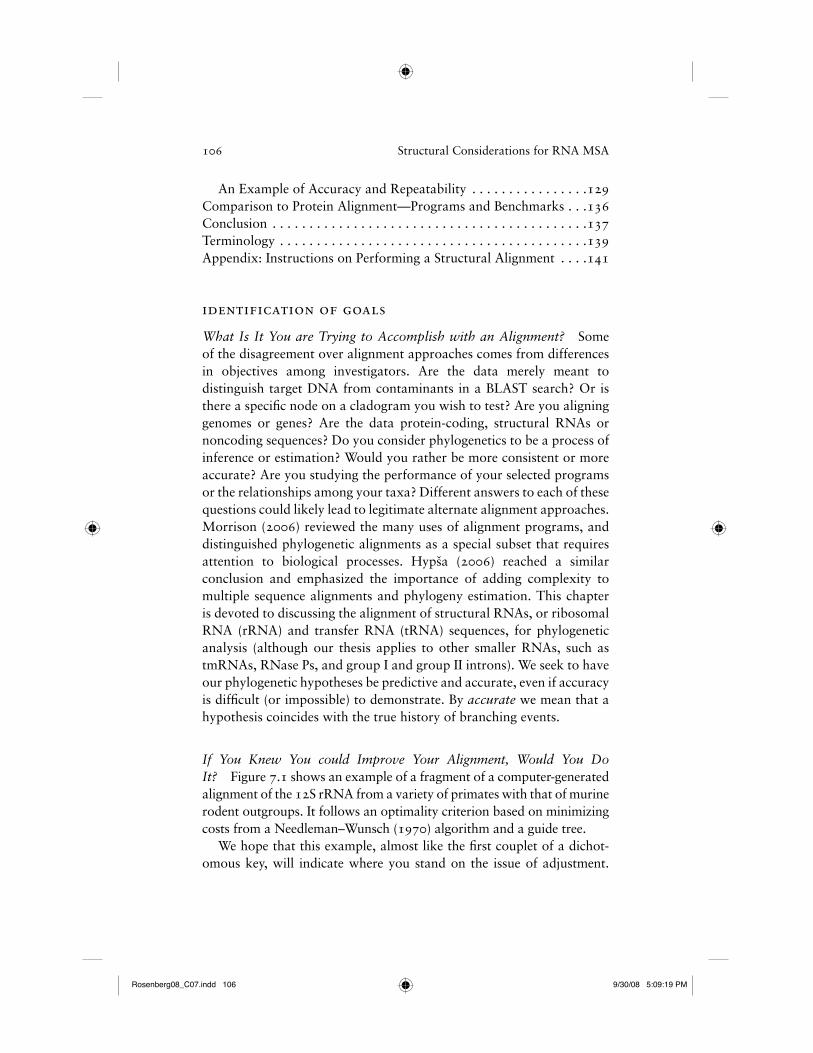
If You Knew You could Improve Your Alignment, Would You Do It? Figure 7.1 shows an example of a fragment of a computer-generated alignment of the 12S rRNA from a variety of primates with that of murine rodent outgroups. It follows an optimality criterion based on minimizing costs from a Needleman–Wunsch (1970) algorithm and a guide tree.
We hope that this example, almost like the fi rst couplet of a dichot-omous key, will indicate where you stand on the issue of adjustment.
Rosenberg08_C07.indd 106Rosenberg08_C07.indd 106 9/30/08 5:09:19 PM9/30/08 5:09:19 PM
Structural Considerations for RNA MSA 107
Notice the “CTTCAGAAAAC” in the middle of the fi gure for both the baboon and the orangutan. If these were your data, would you adjust the sequences to correct the errors made by the program, or would you leave it alone and let the program make all of the decisions about homology, even when it appears to have erred? Would you adjust the nearly identical sequences between the human and the chimps? Would you make decisions about which nucleotides to exclude? Would it bother you if the baboon grouped inside the rodents? There are no correct answers, and the choices you make have implications that relate to what you wish to discover from your data, and tell a lot about both your background and your objectives. If you adjust the alignment, even in this one instance, you have converted to a manual alignment, with all its strengths and limitations. Adjusting the alignment is an attempt to improve the accuracy of an alignment. Here we defi ne “accurate” as representing true (unknowable) homology, and also propose that accu-rate homology estimations will probably improve the accuracy of the phylogenetic hypothesis. But how do you know what “accurate” is, and where do you draw the line? Is manual alignment an art form subject to the whims and biases of the aligner, or can we identify a repeatable meth-odology? Similarly, if we criticize manual alignments as subjective and inconsistent, might these same criticisms apply to computer-generated alignments? If accuracy is a concern, where do current algorithms fail?
Many workers could legitimately state that we cannot objectively defi ne errors made by the computer, and, in fact, the whole concept would be counter to an optimality-based study. If you are looking for the shortest tree, you should favor an alignment that reduces the number of steps. Others might assume that a few errors, even if they
MouseRatGibbonBaboonOrangutanHumanBonoboChimp
GCTACATTTTCTTA--TAAAAGAACAT-TACTATACCCTTTATGAGCTACATTTTCTTTTCCCAGAGAACAT-TACGAAACCCTTTATGAGCTACATTTTCTA--TGCC-AGAAAAC-CACGATAACCCTCATGAGCTACATTTTCTA--CTTCAGAAAACCCCACGATAGCTCTTATGAGCTACATTTTCTA---CTTCAGAAAAC-TACGATAGCCCTCATGAGCTACATTTTCTA---CCCCAGAAAAC-TACGATAGCCCTTATGAGCTACATTTTCTA--CCCC-AGAAAAT-TACGATAACCCTTATGAGCTACATTTTCTA--CCCC-AGAAAAT-TACGATAACCCTTATGA
Figure 7.1. A fragment of an alignment of complete 12S rRNA, generated by ClustalX (Jeanmougin et al. 1998; Thompson et al. 1997).
Rosenberg08_C07.indd 107Rosenberg08_C07.indd 107 9/30/08 5:09:19 PM9/30/08 5:09:19 PM
108 Structural Considerations for RNA MSA
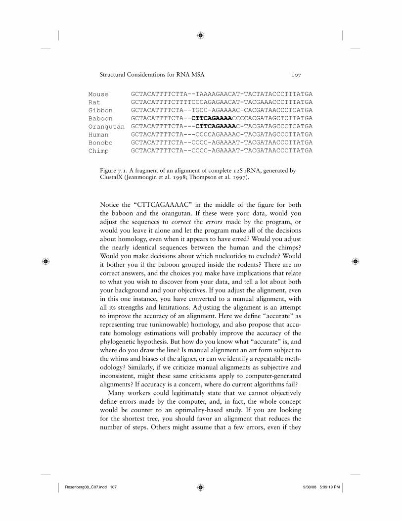
could be defi ned, would be better left alone, because the mass of the data should counterbalance a few random errors. But what if the errors are not random, creating a potential for linking together unrelated groups that share the same systematic biases? What if there were some higher order of conservation that we could examine in making deci-sions about homology that does not necessarily result in shorter trees? Figure 7.2 shows the same region of rRNA as in Figure 7.1, but has been adjusted to minimize secondary structural changes predicted for this region of the molecule. Minimizing structural change is also an optimality criterion for homology assessment that we support and will explore in this chapter. Structural homology is based on position and connection, and assumes that the same structure existed in a common ancestor. Strict adherence to nucleotide homology may require that the same nucleotide state exists in a common ancestor as in its descendants, and, by this defi nition, structural homology and nucleotide homology may support different alignments.
alignment and its relation to data exclusion
One of the things that are not clear from the above comparisons (Figures 7.1 and 7.2) is what we should do with the nucleotides in the “loop” portion of the hairpin-stem loop, between the “TTCT” and the “AGAA.” This is an extremely important issue, but somewhat out-side the debate about alignment. Frequently, these regions are excluded from the analysis on the grounds that they are too variable to align. Some systematists fi nd any form of data exclusion to be unacceptable,
MouseRatGibbonBaboonOrangutanHumanBonoboChimp
GCTACATT(TTCT TATA--AA AGAA)CAT--TACTATACCCTTTATGAGCTACATT(TTCT TTTCCCAG AGAA)CAT--TACGAAACCCTTTATGAGCTACATT(TTCT -ATGCC-- AGAA)AAC--CACGATAACCCTCATGAGCTACATT(TTCT -ACTTC-- AGAA)AACCCCACGATAGCTCTTATGAGCTACATT(TTCT -ACTTC-- AGAA)AAC--TACGATAGCCCTCATGAGCTACATT(TTCT -ACCCC-- AGAA)AAC--TACGATAGCCCTTATGAGCTACATT(TTCT -ACCCC-- AGAA)AAT--TACGATAACCCTTATGAGCTACATT(TTCT -ACCCC-- AGAA)AAT--TACGATAACCCTTATGA
Figure 7.2. A structurally adjusted alignment of the same data as shown in Figure 7.1. Parentheses indicate the bounds of a hairpin-stem loop, with hydrogen-bonded nucleotides indicated with underlines (Kjer et al. 1994). An unaligned region (the “loop” portion of the hairpin-stem) is delimited with spaces.
Rosenberg08_C07.indd 108Rosenberg08_C07.indd 108 9/30/08 5:09:19 PM9/30/08 5:09:19 PM
Structural Considerations for RNA MSA 109
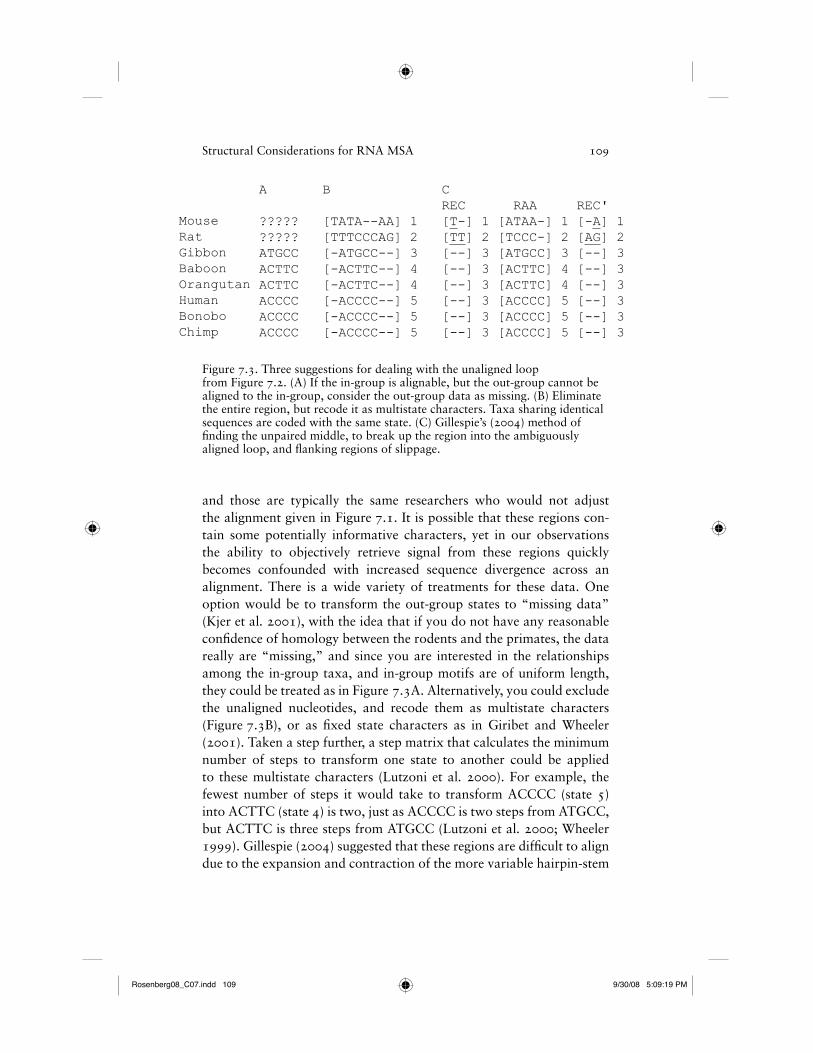
and those are typically the same researchers who would not adjust the alignment given in Figure 7.1. It is possible that these regions con-tain some potentially informative characters, yet in our observations the ability to objectively retrieve signal from these regions quickly becomes confounded with increased sequence divergence across an alignment. There is a wide variety of treatments for these data. One option would be to transform the out-group states to “missing data” (Kjer et al. 2001), with the idea that if you do not have any reasonable confi dence of homology between the rodents and the primates, the data really are “missing,” and since you are interested in the relationships among the in-group taxa, and in-group motifs are of uniform length, they could be treated as in Figure 7.3A. Alternatively, you could exclude the unaligned nucleotides, and recode them as multistate characters (Figure 7.3B), or as fi xed state characters as in Giribet and Wheeler (2001). Taken a step further, a step matrix that calculates the minimum number of steps to transform one state to another could be applied to these multistate characters (Lutzoni et al. 2000). For example, the fewest number of steps it would take to transform ACCCC (state 5) into ACTTC (state 4) is two, just as ACCCC is two steps from ATGCC, but ACTTC is three steps from ATGCC (Lutzoni et al. 2000; Wheeler 1999). Gillespie (2004) suggested that these regions are diffi cult to align due to the expansion and contraction of the more variable hairpin-stem
A B C REC RAA REC'????? [TATA--AA] 1 [T-] 1 [ATAA-] 1 [-A] 1 ????? [TTTCCCAG] 2 [TT] 2 [TCCC-] 2 [AG] 2 ATGCC [-ATGCC--] 3 [--] 3 [ATGCC] 3 [--] 3 ACTTC [-ACTTC--] 4 [--] 3 [ACTTC] 4 [--] 3 ACTTC [-ACTTC--] 4 [--] 3 [ACTTC] 4 [--] 3 ACCCC [-ACCCC--] 5 [--] 3 [ACCCC] 5 [--] 3 ACCCC [-ACCCC--] 5 [--] 3 [ACCCC] 5 [--] 3 ACCCC [-ACCCC--] 5 [--] 3 [ACCCC] 5 [--] 3
MouseRatGibbonBaboonOrangutanHumanBonoboChimp
Figure 7.3. Three suggestions for dealing with the unaligned loop from Figure 7.2. (A) If the in-group is alignable, but the out-group cannot be aligned to the in-group, consider the out-group data as missing. (B) Eliminate the entire region, but recode it as multistate characters. Taxa sharing identical sequences are coded with the same state. (C) Gillespie’s (2004) method of fi nding the unpaired middle, to break up the region into the ambiguously aligned loop, and fl anking regions of slippage.
Rosenberg08_C07.indd 109Rosenberg08_C07.indd 109 9/30/08 5:09:19 PM9/30/08 5:09:19 PM
110 Structural Considerations for RNA MSA
loops of rRNA. He proposed a method that defi nes regions of ambigu-ous alignment, slippage, and regions of expansion and contraction (called RAA/RSC/REC coding), which subdivides these ambiguous regions based on their structural properties and is directly applicable to the methods of Kjer et al. (2001) and Lutzoni et al. (2000). A demon-stration of three alternative treatments is shown in Figure 7.3C.
differentiation of molecules
It is obvious that the selective processes involved in the effects of insertions or deletions (indels) on the function of a gene (and thus the probability of observing such a change in a living organism) are completely different for structural RNAs and protein-coding genes. An indel of one or two nucleotides in a protein-coding gene results in a reading frame shift, whereas an indel of even three nucleotides adds or subtracts a codon. Thus, a single indel will most likely have a major effect on protein structure and function. Indels in structural RNA genes are very different. The effect an indel has on structural RNA is variable across sites of the gene. For instance, some regions of rRNA are highly conserved in length across phylogenetic domains whose common ancestors stretch back for billions of years (Gutell 1996), implying that there is little or no tolerance for length variation in these regions of a functional ribosome. Other regions freely tolerate insertions and dele-tions, as observed among the most recently divergent species (Schnare et al. 1996). So the location of indels, their frequency, and their length in ribosomal RNAs are determined by the affects they have on rRNA structure and hence function. Indels in rRNA are not randomly dis-tributed, but typically highly clustered into regions called expansion segments (or variable regions) that are much reduced, or nonexistent, in prokaryotes and lower eukaryotes. These expansion segments are located on the surface of the ribosome in regions not considered critical for ribosome function (Ban et al. 2000; Cate et al. 1999; Schluenzen et al. 2000; Spahn et al. 2001; Wimberly et al. 2000; Yusupov et al. 2001); thus their evolution can be considered less constrained than that of the core rRNA.
There are other differences in alignment protocols that are dependent on the kinds of questions an investigator is attempting to answer. Researchers who study the evolution of genes need to look at structural variation. Information about how a protein evolves across kingdoms includes major rearrangements, missing amino acids, and
AUQ1
Rosenberg08_C07.indd 110Rosenberg08_C07.indd 110 9/30/08 5:09:20 PM9/30/08 5:09:20 PM
Structural Considerations for RNA MSA 111
large insertions, which may make alignment more diffi cult. At the level where we observe major substitution of codons, there is often a coinci-dent saturation of nucleotides, typically at the fi rst and second codon positions. On the other end of the spectrum, if you are a population geneticist looking for patterns among recently diverged populations, you may encounter variation in noncoding regions of the genome. So investigators at both the deepest and the shallowest levels of divergence may confront serious alignment problems that we do not address in this chapter. An alignment of a protein-coding gene with so many indels that render homology assignment ambiguous is probably not an ideal marker for phylogenetic studies (note, for example, how many phylo-genetic papers state that their protein-coding genes were length invari-ant, or that alignment was trivial). Similarly, noncoding regions, such as introns, are relatively rare sources for estimating phylogenies. So, for phylogenetic systematists, alignment problems are most frequently encountered with rRNAs or tRNAs. Those who design alignment algo-rithms are often interested in serving all investigators, however, and many programs are specifi cally designed to align proteins, with the default parameters set for protein-coding genes. All of these statements seem intuitively obvious. Yet, how many times in the literature have we seen phylogenetic studies state in their methods sections that rRNAs were aligned with default parameters, that is, using a program whose defaults were set to align proteins? There seems to be a basic misunder-standing, or at least a lack of concern, about differentiating alignment processes according to the effect that indels have on the kinds of genes that are being aligned (but see Benavides et al. 2007). We fi nd a discon-nection between alignment philosophy and biological and evolutionary constraints. Does constructing an alignment based on maximizing nucleotide identity make sense for rRNA?
rRNA Sequences Evolve under Structural Constraints
That nucleotides in rRNA do not evolve parsimoniously can be unam-biguously demonstrated. Put another way, rRNA structures change more slowly than do the nucleotides that they comprise. The Gutell laboratory (http://www.rna.icmb.utexas.edu/) maintains a database, the Comparative RNA Web Site (Cannone et al. 2002), from which secondary structural diagrams can be downloaded. To demonstrate the nonconservation of nucleotides, relative to structural features, we suggest you download and print any two structural diagrams
Rosenberg08_C07.indd 111Rosenberg08_C07.indd 111 9/30/08 5:09:20 PM9/30/08 5:09:20 PM
112 Structural Considerations for RNA MSA
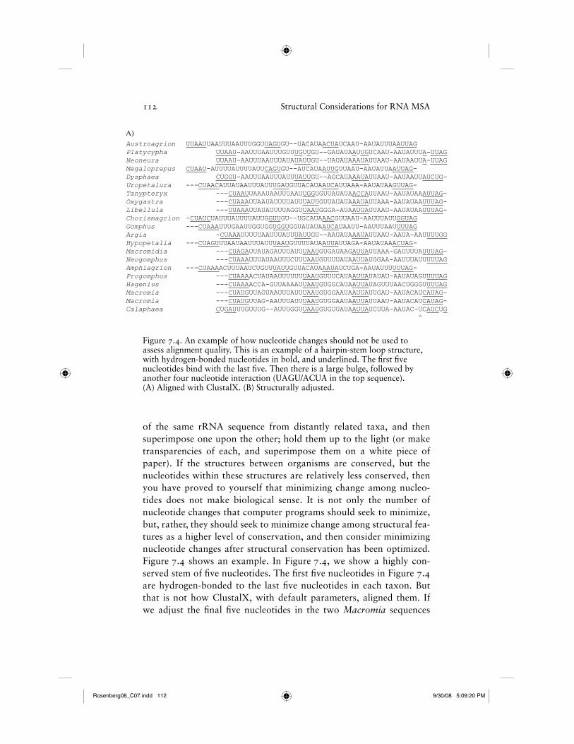
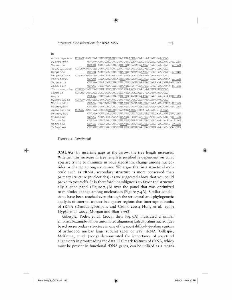
of the same rRNA sequence from distantly related taxa, and then superimpose one upon the other; hold them up to the light (or make transparencies of each, and superimpose them on a white piece of paper). If the structures between organisms are conserved, but the nucleotides within these structures are relatively less conserved, then you have proved to yourself that minimizing change among nucleo-tides does not make biological sense. It is not only the number of nucleotide changes that computer programs should seek to minimize, but, rather, they should seek to minimize change among structural fea-tures as a higher level of conservation, and then consider minimizing nucleotide changes after structural conservation has been optimized. Figure 7.4 shows an example. In Figure 7.4, we show a highly con-served stem of fi ve nucleotides. The fi rst fi ve nucleotides in Figure 7.4 are hydrogen-bonded to the last fi ve nucleotides in each taxon. But that is not how ClustalX, with default parameters, aligned them. If we adjust the fi nal fi ve nucleotides in the two Macromia sequences
Austroagrion UUAAUUAAUUUAAUUUGGUUAGUGU--UACAUAACUAUCAAU-AAUAUUUAAUUAGPlatycypha UUAAU-AAUUUAAUUUGUUUGUUGU--GAUAUAAUUGUCAAU-AAUAUUUA-UUAGNeoneura UUAAU-AAUUUAAUUUAUAUAUUGU--UAUAUAAAUAUUAAU-AAUAAUUA-UUAGMegaloprepus CUAAU-AUUUUAUUUUAUUCAGUGU--AUCAUAAUUGUUAAU-AAUAUUAAUUAG-Dysphaea CUGGU-AAUUUAAUUUAUUUAUUGU--AGCAUAAAUAUUAAU-AAUAAUUAUCUG-Uropetalura ---CUAACAUUAUAAUUUAUUUGAUGUUACAUAAUCAUUAAA-AAUAUAAGUUAG-Tanypteryx ---CUAAUUAAAUAAUUUAAUUGGUGUUAUAUAACCAUUAAU-AAUAUAAAUUAG-Oxygastra ---CUAAAUUAAUAUUUUAUUUAUUGUUAUAUAAAUAUUAAA-AAUAUAAUUUAG-Libellula ---UUAAAUUAUAUUUUAGGUUAAUGGGA-AUAAUUAUUAAU-AAUAUAAUUUAG-Chorismagrion -CUAUCUAUUUAUUUUAUUGGUUGU--UGCAUAAACGUUAAU-AAUUUAUUGGUAGGomphus ---CUAAAUUUGAAUUGGUGGUGGUGGUAUAUAAUCAUAAUU-AAUUUAAUUUUAGArgia -CUAAAUUUUUAAUUUAUUUAUUGU--AAUAUAAAUAUUAAU-AAUA-AAUUUUGGHypopetalia ---CUAGUUUAAUAAUUUAUUUAAUGUUUUAUAAUUAUUAGA-AAUAUAAACUAG-Macromidia ---CUAGAUUAUAGAUUUAUUUAAUGUGAUAAGAUUAUUAAA-GAUUUUAUUUAG-Neogomphus ---CUAAAUUUAUAAUUUCUUUAAUGUUUUAUAAUUAUGGAA-AAUUUAUUUUUAGAmphiagrion ---CUAAAACUUUAAUCUGUUUAUUGUUACAUAAAUAUCUGA-AAUAUUUUUUAG-Progomphus ---CUAAAACUAUAAUUUUUUUAAUGUUUCAUAAUUAUAUAU-AAUAUAGUUUUAGHagenius ---CUAAAACCA-GUUAAAAUUAAUGUGGCAUAAUUAUAGUUUAACUGGGUUUUAGMacromia ---CUAUGUUAGUAAUUUAUUUAAUGUGGAAUAAUUAUUGAU-AAUACAUCAUAG-Macromia ---CUAUGUUAG-AAUUUAUUUAAUGUGGAAUAAUUAUUAAU-AAUACAUCAUAG-Calaphaea CUGAUUUGUUUG--AUUUGGUUAAUGUGUUAUAAUUAUCUUA-AAUAC-UCAUCUG ^
A)
Figure 7.4. An example of how nucleotide changes should not be used to assess alignment quality. This is an example of a hairpin-stem loop structure, with hydrogen-bonded nucleotides in bold, and underlined. The fi rst fi ve nucleotides bind with the last fi ve. Then there is a large bulge, followed by another four nucleotide interaction (UAGU/ACUA in the top sequence). (A) Aligned with ClustalX. (B) Structurally adjusted.
Rosenberg08_C07.indd 112Rosenberg08_C07.indd 112 9/30/08 5:09:20 PM9/30/08 5:09:20 PM
Structural Considerations for RNA MSA 113
(CAUAG) by inserting gaps at the arrow, the tree length increases. Whether this increase in tree length is justifi ed is dependent on what you are trying to minimize in your algorithm: change among nucleo-tides or change among structures. We argue that in a structural mol-ecule such as rRNA, secondary structure is more conserved than primary structure (nucleotides) (as we suggested above that you could prove to yourself). It is therefore unambiguous to favor the structur-ally aligned panel (Figure 7.4B) over the panel that was optimized to minimize change among nucleotides (Figure 7.4A). Similar conclu-sions have been reached even through the structural and phylogenetic analysis of internal transcribed spacer regions that interrupt subunits of rRNA (Denduangboripant and Cronk 2001; Hung et al. 1999; Hypša et al. 2005; Morgan and Blair 1998).
Gillespie, Yoder, et al. (2005, their Fig. 9A) illustrated a similar empirical example of how automated alignment failed to align nucleotides based on secondary structure in one of the most diffi cult-to-align regions of arthropod nuclear large subunit (LSU or 28S) rRNA. Gillespie, McKenna, et al. (2005) demonstrated the importance of structural alignments in proofreading the data. Hallmark features of rRNA, which must be present in functional rDNA genes, can be utilized as a means
Austroagrion UUAAUUAAUUUAAUUUGGUUAGUGUUACAUAACUAUCAAU-AAUAUUUAAUUAGPlatycypha UUAAU-AAUUUAAUUUGUUUGUUGUGAUAUAAUUGUCAAU-AAUAUUU-AUUAGNeoneura UUAAU-AAUUUAAUUUAUAUAUUGUUAUAUAAAUAUUAAU-AAUAAUU-AUUAGMegaloprepus CUAAU-AUUUUAUUUUAUUCAGUGUAUCAUAAUUGUUAAU-AAUA-UUAAUUAGDysphaea CUGGU-AAUUUAAUUUAUUUAUUGUAGCAUAAAUAUUAAU-AAUAAUU-AUCUGUropetalura CUAAC-AUUAUAAUUUAUUUGAUGUUACAUAAUCAUUAAA-AAUAUAA-GUUAGTanypteryx CUAAU-UAAAUAAUUUAAUUGGUGUUAUAUAACCAUUAAU-AAUAUAA-AUUAGOxygastra CUAAA-UUAAUAUUUUAUUUAUUGUUAUAUAAAUAUUAAA-AAUAUAA-UUUAGLibellula UUAAA-UUAUAUUUUAGGUUAAUGGGA-AUAAUUAUUAAU-AAUAUAA-UUUAGChorismagrion CUAUC-UAUUUAUUUUAUUGGUUGUUGCAUAAACGUUAAU-AAUUUAUUGGUAGGomphus CUAAA-UUUGAAUUGGUGGUGGUGGUAUAUAAUCAUAAUU-AAUUUAAUUUUAGArgia CUAAA-UUUUUAAUUUAUUUAUUGUAAUAUAAAUAUUAAU-AAUA-AAUUUUGGHypopetalia CUAGU-UUAAUAAUUUAUUUAAUGUUUUAUAAUUAUUAGA-AAUAUAA-ACUAGMacromidia CUAGA-UUAUAGAUUUAUUUAAUGUGAUAAGAUUAUUAAA-GAUUUUA-UUUAGNeogomphus CUAAA-UUUAUAAUUUCUUUAAUGUUUUAUAAUUAUGGAA-AAUUUAUUUUUAGAmphiagrion CUAAA-ACUUUAAUCUGUUUAUUGUUACAUAAAUAUCUGA-AAUAUUU-UUUAGProgomphus CUAAA-ACUAUAAUUUUUUUAAUGUUUCAUAAUUAUAUAU-AAUAUAGUUUUAGHagenius CUAAA-ACCA-GUUAAAAUUAAUGUGGCAUAAUUAUAGUUUAACUGGGUUUUAGMacromia CUAUG-UUAGUAAUUUAUUUAAUGUGGAAUAAUUAUUGAU-AAUACAU-CAUAGMacromia CUAUG-UUAG-AAUUUAUUUAAUGUGGAAUAAUUAUUAAU-AAUACAU-CAUAGCalaphaea CUGAUUUGUUUGAUUUGGUUAAUGUGUUAUAAUUAUCUUA-AAUAC-UCAUCUG
B)
Figure 7.4. (continued)
Rosenberg08_C07.indd 113Rosenberg08_C07.indd 113 9/30/08 5:09:20 PM9/30/08 5:09:20 PM
114 Structural Considerations for RNA MSA
of checking the accuracy of generated sequences in a fashion that is no different than using translated amino acid sequences to validate the correct reading frame within protein-coding genes (Gillespie, McKenna, et al. 2005).
challenges to existing programs
Compositional Bias Presents a Severe Challenge
One of the appealing things about DNA data is that all of the character states are discrete. With morphological characters, it often seems that as you continue to study more representatives of a taxon, your formerly “good” or “discrete” characters dissolve into a grade of continuous variation. Nucleotide characters are what they are, without intermedi-ates. Even though this property of four discrete character states, evolving under a common mechanism, enhances the justifi cation for models and algorithmic alignments, it also presents some new problems with homo-plasy due to limited character-state space (Brooks and McLennan 1994; Lanyon 1988; Mishler et al. 1988). If a nucleotide is free to fl icker back and forth among these four states, and if there is some nonrandom bias in the data among independent lineages, then there is the possibility for systematic error in our hypotheses of phylogeny. If life on some other planet had fi ve nucleotides instead of four, then this problem would not be as serious as it is here on earth. If we had only two nucleotide states, this problem would be much worse. Unfortunately, there are biological systems in which there are effectively only two states. For example, arthropod mitochondrial genomes are notoriously AT rich, but this bias ranges from 65.6% in Reticulitermes (Isoptera) to 86.7% in Melipona (Hymenoptera) (Cameron and Whiting 2007). It is easy to predict that with A’s and T’s constituting nearly 87% of the genome, a particular site that can be an A or T (such as silent third and fi rst codon sites), will be. So, taxa that have independently evolved similar compositional biases may be drawn together by rapidly evolving, meaningless sites, and this convergence is more likely with two states than it is with four (Meyer 1994). Simmons et al. (2004) discuss at length the problem of limited character-state space.
Nucleotide compositional bias is particularly problematic in the hypervariable regions of rRNA. The conserved core (the length- invariant, alignment trivial regions) may possess the four nucleotides in nearly equal proportions, whereas the hypervariable regions (which contain many if not most of the parsimony informative characters, and
AUQ2
AUQ3AUQ4
Rosenberg08_C07.indd 114Rosenberg08_C07.indd 114 9/30/08 5:09:20 PM9/30/08 5:09:20 PM
Structural Considerations for RNA MSA 115
wherein different alignment methods produce different hypotheses) can possess extreme nucleotide compositional bias. This bias can vary a great deal among taxa. For example, analyzing the structural proper-ties of nuclear 18S rRNA across the major lineages of insects, Gillespie, McKenna, et al. (2005) demonstrated that base compositional bias within nearly all variable regions was severe, and that the patterns of these biases were inconsistent with phylogenetic expectations. Interest-ingly, in instances where pairwise comparisons of base composition were not signifi cantly different, length heterogeneity was signifi cantly different. This suggests that variable sequence length alone is not the only problem encountered in the alignment of rRNA sequences. Base compositional bias is another confounding factor.
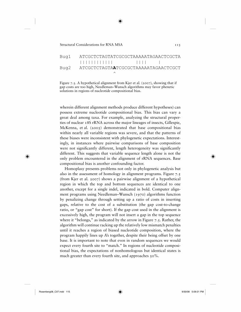
Homoplasy presents problems not only in phylogenetic analysis but also in the assessment of homology in alignment programs. Figure 7.5 (from Kjer et al. 2007) shows a pairwise alignment of a hypothetical region in which the top and bottom sequences are identical to one another, except for a single indel, indicated in bold. Computer align-ment programs using Needleman–Wunsch (1970) algorithms function by penalizing change through setting up a ratio of costs in inserting gaps, relative to the cost of a substitution (the gap cost-to-change ratio, or “gap cost” for short). If the gap cost used in the alignment is excessively high, the program will not insert a gap in the top sequence where it “belongs,” as indicated by the arrow in Figure 7.5. Rather, the algorithm will continue racking up the relatively low mismatch penalties until it reaches a region of biased nucleotide composition, where the program happily lines up A’s together, despite their being offset by one base. It is important to note that even in random sequences we would expect every fourth site to “match.” In regions of nucleotide composi-tional bias, the expectations of nonhomologous but identical states is much greater than every fourth site, and approaches 50%.
Figure 7.5. A hypothetical alignment from Kjer et al. (2007), showing that if gap costs are too high, Needleman–Wunsch algorithms may favor phenetic solutions in regions of nucleotide compositional bias.
Bug1 ATCGCTCTAGTATCGCGCTAAAAATAGAACTCGCTA |||||||||||| |||| |Bug2 ATCGCTCTAGTAATCGCGCTAAAAATAGAACTCGCT
^
Rosenberg08_C07.indd 115Rosenberg08_C07.indd 115 9/30/08 5:09:21 PM9/30/08 5:09:21 PM
116 Structural Considerations for RNA MSA
Biased nucleotide regions are reminiscent of the bland uniformity that frustrates morphologists. But by throwing everything into a computer without looking at it, you would miss the fact that, under conditions of high compositional bias combined with rapid evolu-tion and length variation, Needleman–Wunsch algorithms (and their subsequent derivations) can imitate phenetics, wherein taxa are grouped together according to the overall percentages of A’s and T’s, rather than by synapomorphies. The effects of compositional bias can be amplifi ed if nonhomologous nucleotides are fi rst aligned together with parsimony (with Needleman–Wunsch, minimizing nucleotide change), and then subject to long-branch attraction under a parsimony search. This is why we reject the assertion that alignments and analyses should logically be conducted under the same optimality criterion (Phillips et al. 2000). We believe that the goals of each endeavor (alignment and analysis), while not independent of one another, are different enough to require a different approach, with each step favoring the best option. Simmons (2004) provides a detailed discussion on the separation of homology and analysis. The regions of rRNA that most commonly accumulate extreme compositional bias are the same regions that are most length heterogeneous, and hard to align. Compositional bias presents a severe challenge to Needleman–Wunsch-based alignment algorithms.
Compositional bias is particularly problematic for the direct optimi-zation program POY (Gladstein and Wheeler 1999) because it depends on accurate reconstruction of ancestral sequences. Collins et al. (1994) showed that under conditions of nucleotide compositional bias, or accelerated substitution rates, parsimony severely underrepresents the rare states in ancestral reconstructions. The Collins et al. (1994) study employed a series of empirical and simulation studies to show this, and the mathematical proof by Eyre-Walker (1998) confi rmed their fi ndings. Reconstructing ancestral nodes is what POY does, and these studies indicate that results from a POY analysis should be interpreted with caution, and with an understanding of these limitations under conditions that are characteristic of the hard-to-align regions of rRNA.
Gaps Are Not Uniformly Distributed
Not only are substitution rates elevated in the hypervariable regions of rRNA, but also these regions accumulate insertions and deletions at a much more rapid pace than does the “conserved core” (Clark et al. 1984; Hadjiolov et al. 1984; Hogan et al. 1984; Michot et al. 1984).
Rosenberg08_C07.indd 116Rosenberg08_C07.indd 116 9/30/08 5:09:21 PM9/30/08 5:09:21 PM
Structural Considerations for RNA MSA 117
Anyone who has ever attempted to align rRNA data soon recognizes that gaps are clustered in regions. Kjer et al. (2007) measured the clustering of gaps by simply converting all of the nucleotides in a mammalian rRNA dataset into A’s, and all of the gaps into C’s. The among-site rate variation of indels from our so-altered NEXUS fi le was measured on the expected tree using PAUP version 4.0b10 (1998) by estimating the shape of the gamma distribution (Yang 1994). The gamma distribution is best indicated by a value called “alpha,” whose values below 1 indicate seri-ous among-site rate variation. The alpha value was 0.45, confi rming that variation among sites with respect to the frequency of insertions and deletions is indeed highly variable. This clustering of indels has several important ramifi cations with respect to alignment. Most impor-tantly, it means that ideal gap costs should vary among sites (Kjer 1995). Typically, computer alignments are performed with fi xed gap costs. If biological gap costs vary among sites, then all analyses using fi xed gap costs will underrepresent appropriate gap costs at some sites, and over-represent gap costs at others. The “ideal” average gap cost, even if it were algorithmically and objectively defi ned, would be inappropriate for most sites. Kjer et al. (2007) demonstrate this with a fi gure, repro-duced here as Figure 7.6. In Figure 7.6, structure is indicated with Kjer et al.’s (1994) notation on the nucleotides, and Gillespie’s (2004) struc-tural mask above them. The top panel contains a commonly sequenced region of mitochondrial 12S rRNA from a series of murine rodents. The lower panel contains sequences from a considerably more diverse group: a whale, an ape, an ostrich, a lizard, and a snail. Variation in length among the rodents indicates that the gap cost in those regions should be relatively low, just as invariant lengths among the different phyla should indicate the need for a high gap cost. In this region, we can see that the loop portion of stem 42 (variable region V7) should have a low gap cost, allowing for the easy introduction of gaps. Directly down-stream from this hypervariable region is a region of extremely high con-servation in length. Apparently, indels in strand 38’ are not permitted. Even if we cannot quantify gap costs (which we cannot do because they are arbitrary, and they are arbitrary because we do not have realistic models for indels), you can scan across Figure 7.6 and apply fl exible gap costs. For example, the loop between the strands of stem 40 should receive a low gap cost, and the loop between the strands of stem 42, an even lower gap cost. Contrast those low gap costs to the near infi nite gap cost within strand 38' and all the undefi ned gap costs in between for other sites. If you wish to check your own 12S rRNA data for
Rosenberg08_C07.indd 117Rosenberg08_C07.indd 117 9/30/08 5:09:21 PM9/30/08 5:09:21 PM
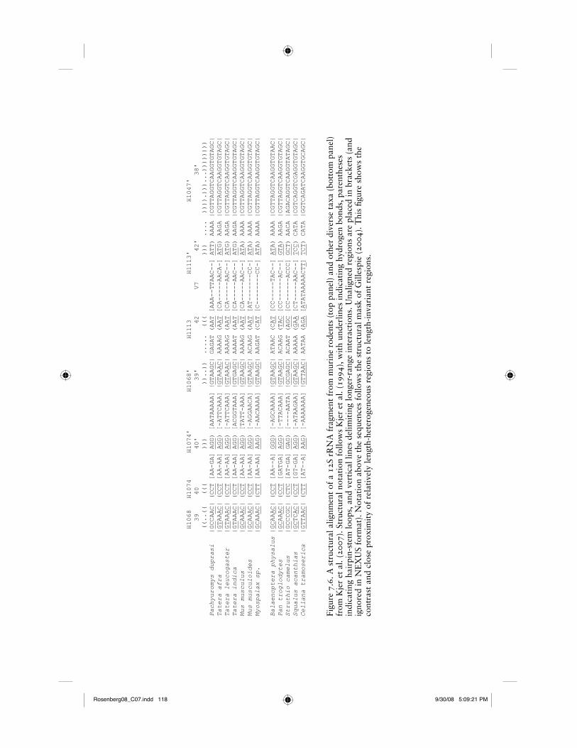
H1068 H1074 H1074' H1068' H1113 H1113' H1047'
39 40 40' 39' 42 V7 42' 38'
((..(( ((( ))) ))..)) ..... ((( ))) .... )))).)))...))))))))
Pachyuromys duprasi |GCCAAC| (CCT [AA-GA] AGG) [AATAAAAA] |GTAAGC| GAGAT (AAT [AAA--TTAAC--] ATT) AAAA |CGTTAGGTCAAGGTGTAGC|
Tatera afra |GTAAAC| (CCT [AA-AA] AGG) [-ATTCAAA] |GTAAAC| AAAAG (AAT [CA-----AACA-] ATG) AAGA |CGTTAGGTCAAGGTGTAGC|
Tatera leucogaster |GTAAAC| (CCT [AA-AA] AGG) [-ATTCAAA] |GTAAAC| AAAAG (AAT [CA-----AAC--] ATG) AAGA |CGTTAGGTCAAGGTGTAGC|
Tatera indica |GTAAAC| (CCT [AA-AA] AGG) [ACGGTAAA] |GTGAGC| AAAAT (AAT [CA-----AAC--] ATG) AAGA |CGTTAGGTCAAGGTGTAGC|
Mus musculus |GCAAAC| (CCT [AA-AA] AGG) [TATT-AAA] |GTAAGC| AAAAG (AAT [CA-----AAC--] ATA) AAAA |CGTTAGGTCAAGGTGTAGC|
Mus musculoides |GCAAAC| (CCT [AA-AA] AGG) [-AGGAACA] |GTAAGC| ACAAG (AAT [AT-------CC-] ATA) AAAA |CGTTAGGTCAAGGTGTAGC|
Myospalax sp. |GCAAAC| (CTT [AA-AA] AAG) [-AACAAAA] |GTAAGC| AAGAT (CAT [C--------CC-] ATA) AAAA |CGTTAGGTCAAGGTGTAGC|
Balaenoptera physalus |GCAAAC| (CCT [AA--A] GGG) [-AGCAAAA] |GTAAGC| ATAAC (CAT [CC-----TAC--] ATA) AAAA |CGTTAGGTCAAGGTGTAAC|
Pan troglodytes |GCAAAC| (CCT [GATGA] AGG) [-TTACAAA] |GTAAGC| ACAAG (TAC [CC------AC--] GTA) AAGA |CGTTAGGTCAAGGTGTAGC|
Struthio camelus |GCCCGC| (CTC [AT-GA] GAG) [----AATA] |GCGAGC| ACAAT (AGC [CC------ACCC] GCT) AACA |AGACAGGTCAAGGTATAGC|
Squalus acanthias |GCTCAC| (CCT [GT-GA] AGG) [-ATAAGAA] |GTAAGC| AAAAA (GAA [CT-----AAC--] TCC) CATA |CGTCAGGTCGAGGTGTAGC|
Cellana tramoserica |GTTAAC| (CTT [AT--A] AAG) [-AAAAAAA] |GTTAAC| AATAA (AGA [ATATAAAAACTT] TCT) CATA |GGTCAGATCAAGGTGCAGC|
Figu
re 7
.6. A
str
uctu
ral a
lignm
ent
of a
12S
rR
NA
fra
gmen
t fr
om m
urin
e ro
dent
s (t
op p
anel
) an
d ot
her
dive
rse
taxa
(bo
ttom
pan
el)
from
Kje
r et
al.
(200
7). S
truc
tura
l not
atio
n fo
llow
s K
jer
et a
l. (1
994)
, wit
h un
derl
ines
indi
cati
ng h
ydro
gen
bond
s, p
aren
thes
es
indi
cati
ng h
airp
in-s
tem
loop
s, a
nd v
erti
cal l
ines
del
imit
ing
long
er-r
ange
inte
ract
ions
. Una
ligne
d re
gion
s ar
e pl
aced
in b
rack
ets
(and
ig
nore
d in
NE
XU
S fo
rmat
). N
otat
ion
abov
e th
e se
quen
ces
follo
ws
the
stru
ctur
al m
ask
of G
illes
pie
(200
4). T
his
fi gur
e sh
ows
the
cont
rast
and
clo
se p
roxi
mit
y of
rel
ativ
ely
leng
th-h
eter
ogen
eous
reg
ions
to
leng
th-i
nvar
iant
reg
ions
.
Rosenberg08_C07.indd 118Rosenberg08_C07.indd 118 9/30/08 5:09:21 PM9/30/08 5:09:21 PM
Structural Considerations for RNA MSA 119
alignment errors, you will probably fi nd them by lining up stem 39. Using fi xed integers as gap costs and applying them across a molecule that is demonstrably length-heterogeneous as a result of regional- specifi c clustering of indels is a commonly used, but biologically unrealistic, approach to the “alignment problem.”
Hence, the practice of exploring parameter space with sensitivity analyses, that is, the testing different gap costs, in an effort to select among an infi nite pool of gap costs and other parameters is problem-atic (but supporters of sensitivity analyses would be correct in noting that this is no more problematic than performing no such tests, if you are tied to fi xed gap costs). Sampling around a series of parameters, as a means of parameter selection, implies that some parameters are “good,” whereas others are “bad.” This is a futile endeavor. There is no ideal, single, fi xed gap cost for an alignment such as this because we are dealing with a heterogeneous assortment of regions. Sensitivity analyses require that at least some of the analyses are appropriate. But when we look at rRNA sequence data, where the “gappy” regions are clustered, we can see that one-gap costs will work well for one region, and poorly for another. By changing the gap cost, other regions may be well aligned, whereas the regions previously well aligned become worse. Different gap costs may shift the appropriately aligned regions from one region to another without necessarily expanding the proportion of well-aligned sites. Of course, if homology is completely ambiguous and unknowable, one may fi nd it useful to present alternative alignments in assessing alignment uncertainty. However, we fi nd it unreasonable to assume that history happened in multiple ways when structural homol-ogy favors a single solution.
One proposal for selecting among parameters is to perform a sen-sitivity analysis on a variety of parameters, and measure each resul-tant tree against some external criterion: a tree based on morphological characters, for example, or minimizing ILD scores (Farris et al. 1994) between partitions. However, there is an infi nite number of parameters to explore. Wheeler (2005) discussed the problem, and also how this infi nite space might be realistically explored. Wheeler (2005) explored gap costs and transversion weights (as did Terry and Whiting 2005; Whiting et al. 1997; and others). These explorations result in a three-dimensional plot of the parameter landscape. What you would want in such a landscape is a single hump containing a distinct peak, because with such a simple distribution, if you are anywhere near the peak, then you can be assured that the combination of gap cost and some other
AUQ5
Rosenberg08_C07.indd 119Rosenberg08_C07.indd 119 9/30/08 5:09:22 PM9/30/08 5:09:22 PM
120 Structural Considerations for RNA MSA
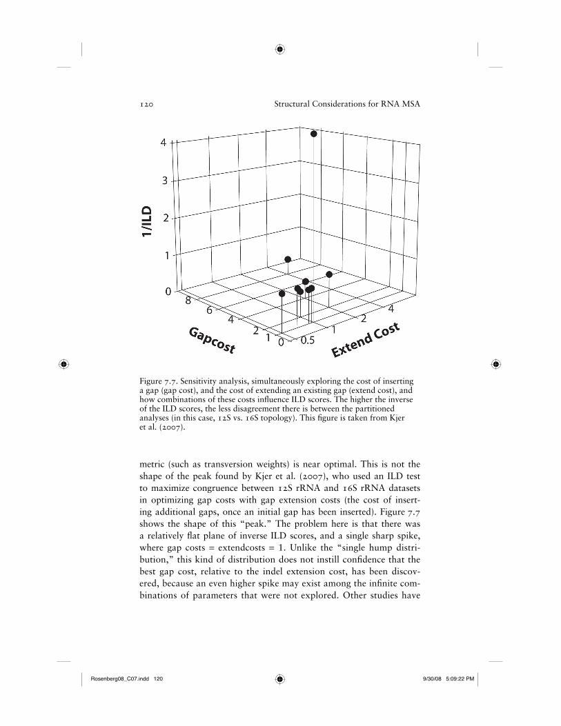
metric (such as transversion weights) is near optimal. This is not the shape of the peak found by Kjer et al. (2007), who used an ILD test to maximize congruence between 12S rRNA and 16S rRNA datasets in optimizing gap costs with gap extension costs (the cost of insert-ing additional gaps, once an initial gap has been inserted). Figure 7.7 shows the shape of this “peak.” The problem here is that there was a relatively fl at plane of inverse ILD scores, and a single sharp spike, where gap costs = extendcosts = 1. Unlike the “single hump distri-bution,” this kind of distribution does not instill confi dence that the best gap cost, relative to the indel extension cost, has been discov-ered, because an even higher spike may exist among the infi nite com-binations of parameters that were not explored. Other studies have
Figure 7.7. Sensitivity analysis, simultaneously exploring the cost of inserting a gap (gap cost), and the cost of extending an existing gap (extend cost), and how combinations of these costs infl uence ILD scores. The higher the inverse of the ILD scores, the less disagreement there is between the partitioned analyses (in this case, 12S vs. 16S topology). This fi gure is taken from Kjer et al. (2007).
Rosenberg08_C07.indd 120Rosenberg08_C07.indd 120 9/30/08 5:09:22 PM9/30/08 5:09:22 PM
Structural Considerations for RNA MSA 121
also found it diffi cult to select parameters with sensitivity analyses (Terry and Whiting 2005; Wheeler 2005), although the generality of this problem has not been explored. One thing is certain, though; it is arbitrary to perform sensitivity analyses that compare only two analyti-cal parameters (such as gap cost vs. transversion weights, or gap costs vs. extend costs) when there are a multitude of interacting parameters that simultaneously infl uence phylogenetic hypotheses. Many of these parameters may not be best treated with integers, or with fi xed values, and many of them, such as the gap cost, are arbitrary (Doyle and Davis 1998; Hickson et al. 2000; Kjer 1995; Phillips et al. 2000; Vingron and Waterman 1994; Wheeler 1996).
Nonindependence of Indels
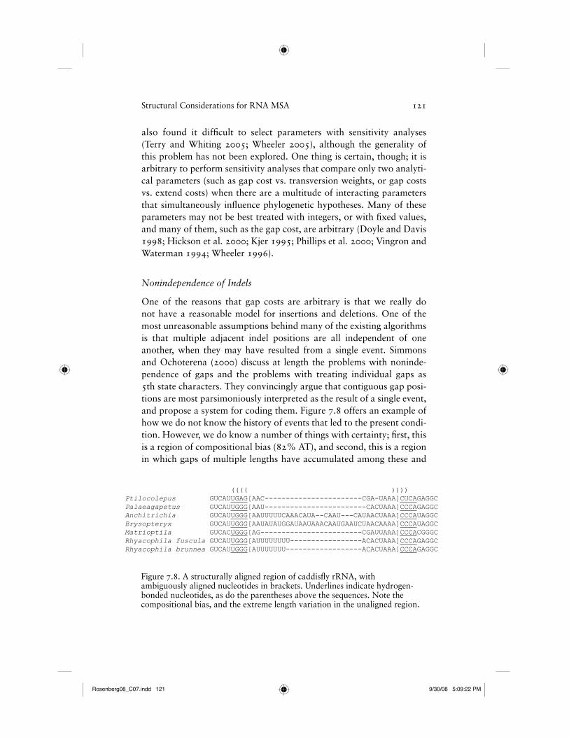
One of the reasons that gap costs are arbitrary is that we really do not have a reasonable model for insertions and deletions. One of the most unreasonable assumptions behind many of the existing algorithms is that multiple adjacent indel positions are all independent of one another, when they may have resulted from a single event. Simmons and Ochoterena (2000) discuss at length the problems with noninde-pendence of gaps and the problems with treating individual gaps as 5th state characters. They convincingly argue that contiguous gap posi-tions are most parsimoniously interpreted as the result of a single event, and propose a system for coding them. Figure 7.8 offers an example of how we do not know the history of events that led to the present condi-tion. However, we do know a number of things with certainty; fi rst, this is a region of compositional bias (82% AT), and second, this is a region in which gaps of multiple lengths have accumulated among these and
(((( )))) Ptilocolepus GUCAUUGAG[AAC-----------------------CGA-UAAA]CUCAGAGGC Palaeagapetus GUCAUUGGG[AAU------------------------CACUAAA]CCCAGAGGC Anchitrichia GUCAUUGGG[AAUUUUUCAAACAUA--CAAU---CAUAACUAAA]CCCAUAGGC Brysopteryx GUCAUUGGG[AAUAUAUGGAUAAUAAACAAUGAAUCUAACAAAA]CCCAUAGGC Matrioptila GUCACUGGG[AG------------------------CGAUUAAA]CCCACGGGC Rhyacophila fuscula GUCAUUGGG[AUUUUUUUU-----------------ACACUAAA]CCCAGAGGC Rhyacophila brunnea GUCAUUGGG[AUUUUUUU------------------ACACUAAA]CCCAGAGGC
Figure 7.8. A structurally aligned region of caddisfl y rRNA, with ambiguously aligned nucleotides in brackets. Underlines indicate hydrogen-bonded nucleotides, as do the parentheses above the sequences. Note the compositional bias, and the extreme length variation in the unaligned region.
Rosenberg08_C07.indd 121Rosenberg08_C07.indd 121 9/30/08 5:09:22 PM9/30/08 5:09:22 PM
122 Structural Considerations for RNA MSA
many other taxa. We also know that this same region is hypervariable and hard to align in a wide range of taxa. In an example taken from caddisfl y (Insecta: Trichoptera) rRNA, we can see that the sequences from Anchitrichia and Brysopteryx (Hydroptilidae, Hydroptilinae) are much longer than those from Paleagepetus and Ptilocolepus (Hydropti-lidae, Ptilocolepinae). If we treat each of the gaps as 5th state characters, that is, as if they were independent of one another, then that would mean that ptilocolepines share 24 independent deletions, relative to Matrioptila. Such a treatment of the data is nonparsimonious. It would be more parsimonious to assume that there was a large insertion of multiple nucleotides in Hydroptilinae, followed by subsequent modi-fi cations. Although the alignment of this region is ambiguous, it gives strong hints about relationships. The nucleotides between the brackets give strong support to the monophyly of Rhyacophila, and the large insert present in the Hydroptilines is likely homologous, since it is long and complex, and there are conserved motifs that indicate a common origin. Yet, for one to infer dozens of synapomorphies from this rapidly changing, unalignable mess, one would have to disregard common sense and assume that all characters are equally informative and independent of one another. Some studies fi nd that 5th state coding for deletions outperform methods that treat deletions as missing data (Ogden and Rosenberg 2007b). While we agree that gaps provide important signals (Freudenstein and Chase 2001), treating them as 5th states falls short to the probability that, while many long inserts do indicate phylogenetic relatedness, treating all the gaps as independent characters infl ates the support for these nodes (Simmons and Ochoterena 2000), whether they are due to common history, convergence, or alignment artifacts.
Long Inserts/Deletions
Whereas simultaneous deletions of fi ve or six nucleotides at a time, occurring in independent lineages, may draw these unrelated taxa together if they are considered to be fi ve or six independent events, much larger indels, sometimes hundreds of nucleotides long, are known to occur (e.g., Giribet and Wheeler 2001 provided a list of atypically long 18S rRNA sequences of metazoans). These long insertions have the potential to wreak havoc on a computer alignment (Benavides et al. 2007). The epitome of this problem is perhaps the bizarre insertions that interrupt both the 28S (Gillespie, unpublished) and 18S (Gillespie, McKenna, et al. 2005) rRNA sequences of the strepsipterans. Not
Rosenberg08_C07.indd 122Rosenberg08_C07.indd 122 9/30/08 5:09:22 PM9/30/08 5:09:22 PM
Structural Considerations for RNA MSA 123
only do inserts occur in the variable regions and expansion segments of the rRNA of these odd insects, but extraordinarily (up to 366 nts.) long insertions are known to occur within the hairpin-stem loop of the highly conserved pseudoknot 13/14 in the V4 region of 18S rRNA (Gillespie, Mcenna, et al. 2005). Thus, despite the earlier statement that conserved regions are less tolerant of indels, the Strepsiptera data suggest that introns can occur in conserved regions. In fact, virtually all of the introns that interrupt rRNAs occur in the most conserved regions of the tertiary structure (Jackson et al. 2002; Wuyts et al. 2001), particularly at the subunit interface or in conserved sites with known tRNA–rRNA interaction (Jackson et al. 2002). While introns are relatively rare in rRNA sequences, only a manual evaluation using a structural model would detect their presence. Still, the majority of large inserts in rRNAs are likely part of the mature molecules and are localized to the surface of the ribosome. However, structural models for the expansion segments and variable regions exposed to the surface of the ribosome are becoming more and more refi ned with the addition of new taxa and sequences and through refi nements in the ribosome crys-tal structures (e.g., Alkemar and Nygård 2003; Alkemar and Nygård 2004; Buckley et al. 2000; Gillespie et al. 2004; Gillespie et al. 2006; Gillespie, McKenna, et al. 2005; Gillespie, Munro, et al. 2005; Gillespie, Yoder, et al. 2005; Hickson et al. 1996; Kjer 1997, 2004; Mears et al. 2006; Misof and Fleck 2003; Ouvrard et al. 2000; Page 2000; Schnare et al. 1996; Wuyts et al. 2000). Thus, conserved structures within even variable regions and expansion segments will be necessary to guide the assignment of nucleotide homology when high levels of length hetero-geneity exist across alignments.
Lack of Recognition of Covarying Sites (A Well-Known, Seldom-Adopted Strategy)
Wheeler and Honeycutt (1988) identifi ed a directed substitution rate within helices of the 5S rRNA of animals and plants that deviates from the neutral theory of molecular evolution explaining rRNA evolution (Kimura 1983; Ohta 1973). This slightly deleterious mode of sequence evolution in rRNA, in which noncanonical base pairings, or bulges, are replaced by compensatory base changes or reversals to the origi-nal state, has been identifi ed in subsequent studies (e.g., Douzery and Catzefl is 1995; Gatesy et al. 1994; Kraus et al. 1992; Rousset et al. 1991; Springer and Douzery 1996; Springer et al. 1995; Vawter and
AUQ6
Rosenberg08_C07.indd 123Rosenberg08_C07.indd 123 9/30/08 5:09:23 PM9/30/08 5:09:23 PM
124 Structural Considerations for RNA MSA
Brown 1993), and appears to be the mechanism orchestrating second-ary structural conservation in rRNAs. Paramount to the fi ndings of Wheeler and Honeycutt (1988) was not only the identifi cation of two different selective constraints within the same molecule (pairing versus nonpairing regions), but also the realization that nucleotides within pair-ing regions in rRNA datasets are not independent characters, because a change at one site infl uences the probability of a substitution at another site. This poses an added diffi culty when treating helices in phylogenetic analysis, as opposed to unpaired nucleotides, wherein interdependence with other positions is not easily demonstrated (although the variety of tertiary and stacking interactions could in theory be modeled). Regard-ing parsimony, analysis of pairing (stems) or nonpairing (loops) regions has been suggested, but not both in simultaneous analysis (Wheeler and Honeycutt 1988). Some workers have implemented a stem-loop weight-ing approach to accommodate the nonindependence of pairing regions (Dixon and Hillis 1993; Smith 1989; Wheeler and Honeycutt 1988). Although seemingly intuitive, down-weighting stems on the basis of their nonindependence will also relatively up-weight positions that are hypervariable, and often nonpairing and perhaps misaligned, thus inac-curately representing the information contained within pairing regions. Up-weighting compensatory mutations within pairing regions has jus-tifi cation (Ouvrard et al. 2000), particularly if rare substitutions defi ne major clades; however, discerning which characters to weight within an alignment can be puzzling if the ancestral pairing cannot be imme-diately identifi ed (i.e., before analysis). Simon (1991) warns against stem-loop weighting, and van de Peer et al. (1993) illustrate that stems and loops are both highly heterogeneous in terms of substitution rates. These added diffi culties, coupled with the fact that assumptions of cer-tain branch support measures such as the bootstrap (Felsenstein 1985) and Bremer support indices (Bremer 1988; Donoghue et al. 1992) are violated by the nonindependence of rRNA pairing regions, suggests that a parsimony approach to analyzing rRNA alignments may not ade-quately accommodate these data. There may be interacting operational vs. philosophical factors involved; if compensatory changes in paired stem sites are also relatively more conservative, parsimony may appropriately (although inadvertently) up-weight the slower-evolving characters (Kjer 2004). Similarly, standard likelihood models of DNA substitution, which are all based on a 4 × 4 rate matrix, are also insuffi cient for phylogeny estimation using rRNA, because of their failure to account for corre-lated bases forming helices.
Rosenberg08_C07.indd 124Rosenberg08_C07.indd 124 9/30/08 5:09:23 PM9/30/08 5:09:23 PM
Structural Considerations for RNA MSA 125
Studies modeling the evolution of pairing regions in rRNA molecules have grown in the last decade. Although most have focused on modeling base pair evolution under likelihood, similar approaches are under development for parsimony (Yoder 2007, Yoder and Gillespie, unpublished). These studies have all centered on implementing a sub-stitution matrix that accommodates the nonindependence of helical regions. Unlike the typical 4 × 4 substitution matrix used for model-ing DNA evolution, a matrix modeling rRNA evolution consists of all possible substitutions within a pairing region. Hence, a 16 × 16 matrix is used to model pairing regions, with the most general time reversible (GTR) model allowing for 134 free parameters. A detailed explana-tion of the simplifi ed families of RNA substitution models was recently provided by Gillespie (2005). Given the attention being addressed to modeling RNA evolution, two software packages have incorporated some of the above-mentioned models into their programs. MrBayes version 3.1 (and earlier versions) (Ronquist and Huelsenbeck 2003) includes model 16B (Schöniger and von Haeseler 1994) and allows for helices to be modeled independently as pairs along with other mod-els for nonpaired sites (i.e., loops, codons, amino acids). Importantly, model 16B should be considered an F81-like model for pairing sites, and when the covarion model in MrBayes is set to REV or HKY85, model 16B becomes different for each case (Jow et al. 2005). The pro-gram PHASE version 1.1 (Jow et al. 2002) also provides a means to simultaneously model multiple partitions with different models of evo-lution. In addition, PHASE contains a suite of RNA models that allow for the evaluation of the performance of different RNA models on a given dataset. Most likely as a result of the study of Savill et al. (2001), those models that allow for base pair asymmetry and a nonzero rate of double substitutions, namely, models 16A, 7A, 7D, 6A, and 6B, are all included in the PHASE program. Thus, PHASE has an appeal over MrBayes 3.1 in that the user can determine the best model of evolution for an RNA dataset, rather than settle for only one RNA model (per-haps with slight modifi cations). The soon-to-be-released MrBayes 4.0 will contain additional rRNA models.
Doublet models are thus directly related to the alignment issue, because alignments performed within a structural context provide a template that allows for a more realistic modeling of the evolution of these complex biological molecules. Intuitively, they are more desirable to the evolutionary biologist. However, it is not our intention here to criticize the algorithmic approach to alignment just because more
Rosenberg08_C07.indd 125Rosenberg08_C07.indd 125 9/30/08 5:09:23 PM9/30/08 5:09:23 PM
126 Structural Considerations for RNA MSA
biologically sound methods exist. On the contrary, we fully support and prefer algorithmic methods, as long as the algorithm that is applied has some grounding in biological reality. Current methods that ignore the properties of rRNA are not biologically grounded. We hope that in pointing out the challenges faced by current methods, we will accelerate the implementation of algorithmic methods, and eventually eliminate the diffi cult, tedious, and nonrepeatable manual alignments. Before this can happen, however, if you favor phylogenetic hypotheses that are mean-ingful and predictive, then manual approaches should not be eliminated until algorithmic methods can be shown to outperform them. Replace-ment should not occur just because a new method remedies some of the problems and is “cool,” new, and computationally expensive.
are structural inferences justified?
One of the criticisms of rRNA structural inferences is that they are inferences, not direct observations. Despite great efforts in cryo-electron microscopy (e.g., Frank and Agrawal 2000; Frank and Agrawal 2001; Frank et al. 2000), complete ribosomal RNA secondary structures can be directly observed only through x-ray crystallography. While several atomic structures of ribosomal subunits now exist for yeast (Spahn et al. 2001), the archaean Haloarcula marismortui (Ban et al. 2000), and the bacteria Thermus thermophilus (Brodersen et al. 2002; Schluenzen et al. 2000; Wimberly et al. 2000; Yusupov et al. 2001) and Deinococcus radiodurans (Harms et al. 2001), most rRNA secondary structures are inferred through comparative evidence. Structural align-ments identify with very high accuracy (>90%, Gutell et al. 2002) those regions involved in base pairing. Comparative evidence works under the assumption that if multiple sequences can fold into the same conserved structure, and if there is a substitution in one part of the putative stem, it is usually followed by its complementary partner. Inferential, yes, but what are the odds that structures are not real, and are you willing to take that chance? The odds that structurally superimposable structures could arise by chance are easily calculable. For example, if there is an A at one site, what is the probability that there will be a T at the position of its putative partner? Answer: 0.25 according to Jukes and Cantor (1969). So if you align two taxa together, and fi nd 35 compensatory mutations between them, the probability of this happening by chance is 0.2535 (that is, a zero, followed by a decimal point, 21 zeros, and then an 8). Adding the thousands of observed compensatory substitutions
Rosenberg08_C07.indd 126Rosenberg08_C07.indd 126 9/30/08 5:09:23 PM9/30/08 5:09:23 PM
Structural Considerations for RNA MSA 127
among all taxa, one arrives at a number so small that the human mind (even among mathematicians who are experienced in thinking about really small numbers) cannot come close to even imagining these num-bers in a meaningful way. When one considers how tenuous the whole process of phylogenetic inference is (where we never know anything, and the best we can do is come up with a reasonable guess, where our data are consistent with our hypotheses, given our assumptions), it seems absurd to argue over whether it is safe to assume whether structural constraints that have a virtually zero (but not technically zero) proba-bility of being random should be abandoned on philosophical (or other) grounds. We also note that translated amino acids are routinely used to check DNA alignments of protein-coding sequences, even though few (if any) of these studies bother to experimentally demonstrate that the genetic code for the taxa of interest is the same as the model taxa.
why align manually?
As we were considering our observations about the objectives of phylogenetic alignment, and beginning to write them down for this paper, Morrison (2006) presented a review of procedures and philosophies. This excellent review thoroughly explores the differences among us, and, in fact, much of what we had thought to be intuitive but unproven could now be explained in a series of logical arguments. Morrison (2006) lays out a series of problems with current algorithms that were designed for one purpose, and then used for phylogenetics. He argues that many of the problems we face in alignments stem from a failure to recognize that the program is neither designed nor suited for phylogenetic inference. Whereas we had noticed these problems, we had assumed that some smart person out there must have some reasonable solution to phylogenetic alignment; we just had not read about it yet. Morrison (2006) presents a radical new view, stating, “Our objective should be biological plausibility rather than mathematical optimality.” With respect to alignments, we are in complete agreement with this statement. Algorithms that currently align sequences with the goal of reaching a mathematical optimum may fail for phyloge-netics if they do not simulate biological reality.
Perceived Advantages of Algorithms
Much about alignment has simply been assumed, without question. One’s preferences, alluded to in the introduction, seem more a matter
AUQ7
Rosenberg08_C07.indd 127Rosenberg08_C07.indd 127 9/30/08 5:09:24 PM9/30/08 5:09:24 PM
128 Structural Considerations for RNA MSA
of culture and tradition than experimentally justifi ed or even thought-fully considered criteria. It seems intuitively obvious that computers are more objective at making alignment decisions than manual alignments. Are they? No, not if the computer requires arbitrary input parameters. The following comparison should be made. Consider a thoughtful sys-tematist, thinking about homology under a series of structural and evo-lutionary constraints. Contrast this to another reasonable systematist, who believes that homology is best decided objectively with a repeatable optimality criterion implemented by a computer. The former may fail through carelessness. The latter may fail when the computer program is actually an irrational black box. Input parameters, such as gap costs, assigned by the investigator determine phylogenetic hypotheses. If these input parameters are arbitrary, then justifying algorithmic approaches over manual ones under a criterion of “objectivity” is almost impossible to argue. One must justify each of the parameters that infl uence the analysis. Yet the argument continues. We believe that if input param-eters are arbitrary and unpredictable, then alignment methods that use them are also arbitrary and unpredictable. To submit one’s data to an algorithm, with no regard for the implications of such an action, is to transfer subjective (and thoughtful) decisions about homology from the human investigator to subjective (and careless) decisions about gap cost determination. Algorithmic methods are not objective if input param-eters are subjectively determined.
Another perceived advantage of algorithmic methods is that they are easier than structural alignments. In our experience, many inves-tigators accept that structural alignments make sense, but they do not make the effort to perform them because they assume that their Clustal alignment is “good enough” and that a few alignment errors gener-ated by the algorithm will be overridden by the mass of signal in their data. We fi nd this cavalier attitude toward homology to be surprising, when we consider the effort and expense that goes into collecting the sequences. In our opinion, it is always worth the effort to align the data with care. As systematists, we are often are more interested in resolving controversial nodes and not so interested in re-corroborating well-established relationships. Controversial internodes are often char-acteristically short, and may be diffi cult to recover by any means with a variety of datasets. It may be that the characters we discard, because the easy method is applied, are the only ones that are informative. Or more likely, the few characters that inform us about a short internode are overwhelmed by a mass of poorly aligned noise. We could never
Rosenberg08_C07.indd 128Rosenberg08_C07.indd 128 9/30/08 5:09:24 PM9/30/08 5:09:24 PM
Structural Considerations for RNA MSA 129
know how a careful alignment would infl uence our results without the effort. Those who support sensitivity analyses to optimize parameters with POY would probably agree with us on this point, as they perform months of analysis time on parallel processors or super clusters. Careful alignment, whether performed by hand or computer, takes time, effort, and expertise. We reject the argument that carefully performed algorith-mic methods are “easier,” and let the reader decide whether “fast and careless” alignments are defendable.
An Example of Accuracy and Repeatability
If algorithmic methods could be shown to be more accurate than man-ual alignments, then we might be able to overlook the possibility that arbitrary parameter selection may sometimes lead to unpredictable hypotheses. This is not the case, however. Many empirical compari-sons have shown that manual alignments tend to recover more reason-able phylogenies (Ellis and Morrison 1995; Gillespie, McKenna, et al. 2005; Hickson et al. 1996; Hickson et al. 2000; Kjer 1995; Kjer 2004; Lutzoni et al. 2000; Morrison and Ellis 1997; Mugridge et al. 2000; Schnare et al. 1996; Titus and Frost 1996; Xia et al. 2003). Phylogenies are hypotheses to be tested, accepted, or refuted by subsequent hypoth-eses. We never “know the truth.” Such hypotheses may be accepted on the grounds that they generally equate to the recovery of expected or corroborated relationships with phylogenetic accuracy. A compelling case can be made for phylogenies generated from manually aligned datasets. Time after time, we recover “more reasonable” phylogenetic hypotheses from carefully aligned data, (while at the same time, analy-ses justifi ed only on epistemological consistency continue to produce “unexpected” hypotheses). Admittedly, these empirical studies can provide only points for discussion. To demonstrate accuracy, we need either known phylogenies from experimentally manipulated systems (such as sampling evolving viruses, Hillis and Bull 1993) or simula-tion studies where we know the history of insertions and deletions in a simulated dataset. However, there are problems with both of these approaches, and these problems stem from the nature of rRNA. Viruses do not possess rRNA, so problems specifi c to rRNA alignment cannot be addressed with manipulated viral sequences. Simulation studies are only as good as the model used to simulate the data. Currently, our abil-ity to model insertions and deletions is limited and unrealistic. Although it is possible to insert gaps into a simulated sequence, any model that
Rosenberg08_C07.indd 129Rosenberg08_C07.indd 129 9/30/08 5:09:24 PM9/30/08 5:09:24 PM
130 Structural Considerations for RNA MSA
assumes that gaps are independent of one another and randomly dis-tributed is not capturing the essence of what is happening in rRNA, where insertions and deletions are frequently multiple nucleotides in lengths, and strongly clustered in variable regions. An accurate model of rRNA evolution would require a proportion of the sites to be cova-rying, gaps to be nonindependent, and substitution rates and length heterogeneity to be regionally variable. Without these characteristic features of rRNA built into the simulation, any generalizations drawn from these studies must be understood to be only crude approxima-tions of biological reality.
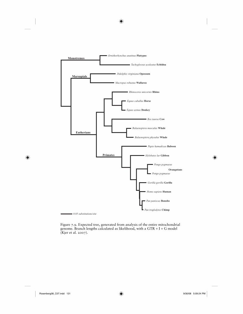
We suggest a reasonable empirical solution to the assessment of accuracy in Kjer et al. (2006, 2007). Although accuracy cannot be fully explored with empirical data, we see at least one example where an “expected tree” is justifi ed. For taxa whose entire mitochondrial genomes are sequenced, it can be expected that partitions of the data share the same history. We suggest that relationships that are corrobo-rated with both nuclear genes and morphology are candidates for iden-tifying sets of phylogenetic expectations from the mitochondrial data. If these independently corroborated nodes are also supported by the combined mitochondrial genome data, then these relationships could be used to assess alignment strategies of any partitions of the data, such as the 12S and 16S mitochondrial rRNAs. Kjer et al. (2007) used the rela-tionships shown in Figure 7.9 to compare phylogenetic accuracy and repeatability of manual and direct optimization methods. These taxa possess complete mitochondrial genome data, and each of the nodes is supported by morphological characters (McKenna and Bell 1997; Novacek 1992; Novacek et al. 1988; Simpson 1945) and nuclear genes (Amrine-Madsen et al. 2003; Delsuc et al. 2002; Waddell and Shelley 2003). The phylogeny shown in Figure 7.9 is recovered from parsi-mony, Bayesian, and Likelihood analyses of the complete mitochon-drial genomes (Gibson et al. 2005; Kjer and Honeycutt 2007; Reyes et al. 2004). One need not accept this as the “true tree,” but merely a tree that is recovered by the entire dataset, and corroborated by mul-tiple independent sources. By defi nition, partitions of the same linked dataset contain less data. It is therefore reasonable to use a tree derived from ten times the number of linked nucleotides in order to test align-ment accuracy. There is a risk to judging an alignment method accord-ing to this sort of phylogenetic expectation. Namely, the risk would be that the “expected tree” was later shown to be inconsistent with a tree derived by some future superior method. As such, the results from
AUQ8AUQ10
AUQ9
Rosenberg08_C07.indd 130Rosenberg08_C07.indd 130 9/30/08 5:09:24 PM9/30/08 5:09:24 PM
Ornithorhynchus anatinus Platypus
Tachyglossus aculeatus Echidna
Didelphis virginiana Opossum
Macropus robustus Wallaroo
Rhinoceros unicornis Rhino
Equus caballus Horse
Equus asinus Donkey
Bos taurus Cow
Balaenoptera musculus Whale
Balaenoptera physalus Whale
Papio hamadryas Baboon
Hylobates lar Gibbon
Pongo pygmaeus
Pongo pygmaeus
Gorilla gorilla Gorilla
Homo sapiens Human
Pan paniscus Bonobo
Pan troglodytes Chimp
0.05 substitutions/site
Orangutans
Monotremes
Marsupials
Eutherians
Primates
Figure 7.9. Expected tree, generated from analysis of the entire mitochondrial genome. Branch lengths calculated as likelihood, with a GTR + I + G model (Kjer et al. 2007).
Rosenberg08_C07.indd 131Rosenberg08_C07.indd 131 9/30/08 5:09:24 PM9/30/08 5:09:24 PM
132 Structural Considerations for RNA MSA
the experiment could be modifi ed by the new phylogenetic expectations. In other words, if one is transparent about how phylogenetic expecta-tions are used to assess alignment performance, then conclusions can easily be overturned with future illumination. Science is about laying out one’s assumptions, and testing hypotheses according to whether or not the data fi t those assumptions.
The experimental design of Kjer et al. (2007) was simple. The 16S rRNA sequences from the taxa shown in Figure 7.9 were assembled, the taxon names were disguised, and the taxon order was shuffl ed within the matrix. The masked data were then sent to three investigators with simple instructions: “Align these data with secondary structure, and also with POY.” It was predicted that if secondary structure could pro-vide a reasonable means of homology assessment, then different inves-tigators would come to similar decisions about structurally infl uenced homology. More simply stated, if the structures were real, we would all fi nd them, and structurally aligned data would lead to similar phylo-genetic conclusions among investigators, because they would be using a nonarbitrary means of homology assessment, even if the alignments themselves were not identical. The second prediction was that if param-eter decisions were arbitrary (Doyle and Davis 1998; Hickson et al. 2000; Kjer 1995; Phillips et al. 2000; Vingron and Waterman 1994; Wheeler 1996), and these parameters had a strong infl uence on phy-logenetic conclusions, then different investigators using an algorithmic approach to a phylogenetic problem would arrive at different phyloge-netic hypotheses, given the same data.
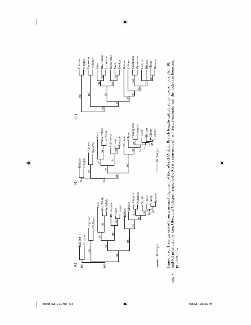
Figure 7.10 shows the results of the experiment. All three of the struc-tural alignments yielded nearly identical results, with the only differ-ence being on the Chimp/Human/Gorilla branch (which is a reasonable refl ection of reality, because this branch has no perceivable length). The structurally aligned data also recovered the expected tree. The hypoth-eses generated from the independent POY analyses (not shown; see Kjer et al. 2007, Fig. 5) resulted in each investigator proposing a different phylogenetic hypothesis, none of which were the expected tree. Each of the POY analyses resulted in different opinions on how to present the confusing array of trees that were generated from the many explorations of alternative parameters. We have already discussed the ambiguity of sensitivity analyses when each of the explorations of parameter space is biologically unrealistic. Alarmingly, even when the same parameters (but not necessarily the same search heuristics) were used, each of the investigators recovered different trees with POY. In all probability, this
Rosenberg08_C07.indd 132Rosenberg08_C07.indd 132 9/30/08 5:09:25 PM9/30/08 5:09:25 PM
Ech
idna
Plat
ypus
A)
B)
C)
100
chan
ges
100
chan
ges
99
99
99
100
100
100 10
0
100
100
100
100
100
100
100
100
100
100 10
0
100
100
100
100
100
10010
0
100
97
100
100
91
89
94
99
5352
57 3998
6339 97
68
49
47
87
86
Opp
osum
Wal
laro
o
Cow
Blu
e W
hale
Fin
Wha
le
Rhi
noce
ros
Hor
se
Don
key
Bab
oon
Gib
bon Ora
ngut
an
Ora
ngut
an
Gor
illa
Chi
mp
Bon
obo
Hum
an
Ech
idna
Plat
ypus
Opp
osum
Wal
laro
o
Cow
Blu
e W
hale
Fin
Wha
le
Rhi
noce
ros
Hor
se
Don
key
Bab
oon
Gib
bon
Ora
ngut
an
Ora
ngut
an
Gor
illa
Chi
mp
Bon
obo
Hum
an
Ech
idna
Plat
ypus
Opp
osum
Wal
laro
o
Cow
Blu
e W
hale
Fin
Wha
le
Rhi
noce
ros
Hor
se
Don
key
Bab
oon
Gib
bon
Ora
ngut
an
Ora
ngut
an
Gor
illa
Chi
mp
Bon
obo
Hum
an
99
Figu
re 7
.10.
Tre
es g
ener
ated
fro
m a
man
ual a
lignm
ent
of t
he 1
6S r
RN
A d
ata.
Bra
nch
leng
ths
calc
ulat
ed w
ith
pars
imon
y. (
A),
(B
),
and
(C)
gene
rate
d by
Kje
r, O
ber,
and
Gill
espi
e, r
espe
ctiv
ely.
(C
) is
a c
onse
nsus
of
two
tree
s. N
umer
als
near
the
nod
es a
re b
oots
trap
pr
opor
tion
s.A
UQ
15
Rosenberg08_C07.indd 133Rosenberg08_C07.indd 133 9/30/08 5:09:25 PM9/30/08 5:09:25 PM
134 Structural Considerations for RNA MSA
was the result of an insuffi cient search strategy. All heuristic exercises, including routine tree searches, can suffer from this problem, and if you start from the same random seed, you will get the same tree. However, direct optimization is more complex than simple tree searches, and fi g-uring out how long to run the analysis is another decision that needs to be made. In this example, structurally aligned data resulted in phyloge-netically identical hypotheses that conformed to the corroborated tree. Is that not what we want in terms of repeatability? Consider the scenario of baking a cake. We follow a recipe: 2 eggs, a cup of fl our, a cup of sugar, and so forth, . . . mix well, and then bake in the oven at 375 °F for 30 minutes. Perhaps one person uses 5% more fl our than another, or one person stirs with greater vigor. Regardless, the end product is a cake. With manual alignments guided by secondary structure, we all get cake in the end (Figure 7.10). Repeatability in science has always been defi ned in this way. We describe the methods, and then see if others can repeat it. Taken even further, if the alignment is presented, the analyses can be precisely repeated, and the decisions that went into it can be assessed and changed. Kjer et al. (2007) show that when you follow the cake recipe, and pop the data into POY, you do not know what will come out; it might be a loaf of bread. Of course, our scenario is one of exaggeration, but it serves to make a point. When you are cooking (or applying math-ematics), you can tell the difference between the end results of a cake and a loaf of bread. In phylogenetics, the end products cannot be so easily distinguished from one another with respect to which is correct.
Not everyone agrees with the generalizations we reported in Kjer et al. (2007), and as with any work, there are, no doubt, legitimate criticisms that we would like people to consider. This work (Kjer et al. 2007) was presented as an opinion piece to foster some discussions about the ambiguities of alignments, both manual and computer gener-ated. We asked one of our critics, Gonzalo Giribet, to summarize the basic weakness of our work here.
I think that we both agree that secondary structure information is valuable for refi ning homology hypotheses but we differ in the way we incorporate such ancillary information into our homology-assignment techniques, being those multiple alignments or simply putative synapomorphies in “direct optimization” techniques (what I have called “single-step phylogenetics”). We have different understanding of what reproducibility may mean, and although I see an alignment as a pure topology-dependant hypothesis you may view it as something that is fundamentally knowable, i.e., that there is “one” alignment. This is what causes that you may search for
Rosenberg08_C07.indd 134Rosenberg08_C07.indd 134 9/30/08 5:09:25 PM9/30/08 5:09:25 PM
Structural Considerations for RNA MSA 135
“the” alignment while I am more interested in exploring what alternative parameter sets may have to do with my homology hypothesis, i.e., assess-ing the stability of my results to alternative parameter sets.
Naturally we do not agree with everything Giribet has to say about sensitivity analysis. There seem to be two purposes for sensitivity anal-yses; one would be to fi nd the most justifi ed set of parameters, and therefore select a favored hypotheses derived from the preferred input parameters. The other purpose would be to explore the stability of the data to a variety of parameters, and present a phylogenetic hypoth-esis that includes measures of alignment uncertainty. Giribet supports the second of these in his statement above, and there may have been instances where we have confused these two justifi cations for sensitivity analyses. We appreciate his effort to clarify this difference, but still fi nd both uses of sensitivity analyses problematic.
We think that phylogenetics is a near impossible enterprise, and the best we can do is to do our best. We should not be ashamed of pursu-ing accuracy, even if it is impossible to assess. We agree with Giribet that sensitivity to alignment uncertainty should be explored, and that uncertainty in an alignment should eventually be part of our estimates of support. We think that this would probably require a Bayesian method, similar to that proposed by Redelings and Suchard (2005).
If one is interested in a “best estimate” of phylogeny, this estimate will likely come from an analysis in which homology (alignment) is optimized. Another area of ambiguity is amplifi ed when multiple align-ment parameters offer many different trees; it becomes diffi cult to infor-matively select among them. The utility of a phylogenetic hypothesis is drastically reduced when no hypothesis can be considered better than another, because all of the trees are devoted to explorations of the data under different alignment input parameters. For example, what can we take from Wheeler et al. (2001) as a phylogenetic hypothesis? Surely not the “discussion tree,” but if not that, should we favor the myriad of other trees that collapse to a near meaningless polytomy? We believe that it is the responsibility on an investigator to clearly present his or her hypothesis. The best way to do so would be to state “the best estimate of phylogeny we could make comes from analysis ‘X,’ shown in Fig. ‘Y.’” It is the responsibility of the reader to then evaluate the results and either agree or disagree with the fi ndings. For this dynamic process to occur, one must present the data, present the alignment, and justify the deci-sions that were made. The current feasibility of justifying one’s decisions
Rosenberg08_C07.indd 135Rosenberg08_C07.indd 135 9/30/08 5:09:25 PM9/30/08 5:09:25 PM
136 Structural Considerations for RNA MSA
with an algorithmic approach is not as straightforward as is the case with a manual approach.
comparison to protein alignment—programs and benchmarks
Protein alignment programs have seen much development in recent years, beginning with ClustalW (Thompson et al. 1994) to current state-of-the-art approaches, such as Probalign (Roshan and Livesay 2006), Probcons (Do et al. 2005), and MAFFT (Katoh et al. 2005). These programs use a variety of techniques, such as hidden Markov models (Durbin et al. 1998), maximal expected accuracy (Durbin et al. 1998), fast Fourier transforms (Katoh et al. 2005), profi le alignment (Edgar 2004a), and consistency alignment (Do et al. 2005). Most protein alignment programs aim to align parts of proteins conserved in sequence or structure. This is facilitated by amino acid substitution-scoring matrices estimated from real data (such as PAM, Dayhoff and Eck 1968; and BLOSUM, Henikoff and Henikoff 1992) and manually created protein alignment benchmarks, also based on real data (such as HOMSTRAD, Mizuguchi et al. 1998b; and BAliBASE, Thompson et al. 2005b). These benchmarks, which are primarily structure-based alignments, not only allow for comparison of different programs, but also enable optimization of gap penalty parameters on real data. As a result, protein alignment programs have shown a steady increase in accu-racy over the years. The most accurate programs use a combination of techniques, such as PSI-BLAST profi les, and predicted secondary struc-tures as found in the PROMALS program (Pei and Grishin 2007).
Most protein sequence alignment programs can be used for RNA align-ment in principle. However, substitution scoring matrices and alignment benchmarks (analogous to BLOSUM and BAliBASE, for example) were not developed for RNA until recently. The BRaliBASE RNA alignment benchmark (Gardner et al. 2005), similar to BAliBASE for proteins, is the fi rst RNA alignment benchmark produced by aligning sequence while taking into consideration secondary structure. Subsequent efforts have expanded BRaliBASE (see Wilm et al. 2006). Yet, BRaliBASE still lacks the size and diversity of its protein counterparts. The RIBOSUM scoring matrices (Klein and Eddy 2003) for RNA are comparable to the BLOSUM matrices for proteins; however, recent studies show that they perform more poorly than simpler scoring matrices when used in the ClustalW program on enhanced BRaliBASE benchmarks (Wilm et al. 2006).
Further development of RNA alignment benchmarks, better substitu-tion scoring matrices, and adaptation of techniques used in state-of-the-art
Rosenberg08_C07.indd 136Rosenberg08_C07.indd 136 9/30/08 5:09:25 PM9/30/08 5:09:25 PM
Structural Considerations for RNA MSA 137
protein alignment programs will eventually lead to better algorithms for aligning RNA. Alignment of conserved regions (in sequence or structure) is accepted as a measure of correctness in the protein domain. In light of our discussion in the preceding sections, the same criteria should apply when aligning RNA.
conclusion
When initially asked to contribute to this book, I thought that we would provide a chapter on the problems with algorithmic methods. However, we fi nd this to be an overly negative approach. We all have different backgrounds—and experience. Sometimes we see things in different ways, and our experience differs greatly from that of many of the other contributors to this book. These differences are a good thing, as differing points of view should be openly discussed and debated. Thus, our science progresses. It is all too easy in science to take an adversarial approach to those who disagree with us. It is not our intention in this chapter to be overly critical. We do support properly invoked algorithmic methods, and clearly stated optimality criteria. It is our hope that, by our pointing out some of the problems we have experienced in the alignment of rRNA data, program developers can incorporate solutions to these issues in their algorithms. Biologically realistic algorithms could make manual alignment less and less relevant. Here are some of the issues we see as most important toward the improvement of alignment programs.
In molecules whose function is dependent on structure, the conserva-tion of the structure should be part of the optimality criterion. Minimizing structural change is as justifi ed as minimizing change among nucleotides. Perhaps a program could be developed that could locate covarying sites in a multiple alignment. Some multistepped combination of calculating minimum free energy structures that are shared among multiple taxa, and then confi rming those hypothesized structural interactions based on compensatory base changes, seems possible. Sites containing such com-pensatory base changes should be aligned together. A research group led by P. Stadler at the University of Leipzig and a research group led by B. Misof at the University of Bonn have developed a promising program called RNAsalsa that promises to do these things (B. Misof, personal communication), but we have not had a chance to evaluate it.
Gap costs should vary among regions. Manual alignments contain fl exible gap costs, in that when a person comes to a hypervariable region with a lot of variation in length among sequences, gaps are more freely inserted. With an algorithm, there should be a way to locate conserved
Rosenberg08_C07.indd 137Rosenberg08_C07.indd 137 9/30/08 5:09:26 PM9/30/08 5:09:26 PM

138 Structural Considerations for RNA MSA
regions by some criteria, and then measure the range of length varia-tion among taxa in the regions between them. Gap costs could then be regionally assigned based on how much length variation was observed, giving the lowest gap costs to regions that contain the most length het-erogeneity. The standard deviation of the lengths could also play a role in gap cost determination, and in data exclusion criteria.
The iterative process of moving from guide trees to multiple alignments should be improved upon. Perhaps the initial guide tree should be devel-oped from unambiguously aligned regions; we could then iteratively move through more diffi cult regions with guide trees developed only from data whose homology reaches some confi dence threshold. It is fairly easy to see by eye when one lineage cannot be aligned with another. Reconstruct-ing ancestral states to the root of a particular lineage may yield sequences so different from other lineages that it would be foolish to attempt to homologize them. If it is that easy to see for the human eye, there should be a way for a computer to measure this incompatibility as well, and reach objective criteria for data exclusion. Gblocks (Castresana 2000) provides a conservative means of data exclusion. Another interesting program called “Aliscore,” based on the identifi cation of randomness in sequence alignments using a Monte Carlo approach, is being developed by Misof and Misof (personal communication). We need more informa-tion about how gaps accumulate and evolve in rRNA to model these characters. The greatest challenge is that gaps are not independent of one another, and are not randomly distributed across sites. Alignment programs must recognize both of these properties.
An ideal program would have a means to assess alignment uncer-tainty (as in Redelings and Suchard 2005). But alignment uncertainty is linked with the model, so it is important to remember that if the model for gaps is biologically unrealistic, then the “uncertainty” cannot be disentangled from those limitations. It is our impression that the differ-ences among trees that are attributed to alignment methods are more often associated with different data exclusion criteria and philosophies. It should be possible to produce a program that incorporates some data exclusion criterion with alignment uncertainty.
Alignments involving moderate to extreme length heterogeneity across sampled sequences will undoubtedly invoke some degree of subjectivity from the investigator, regardless of the methodological approach (Kjer et al. 2007). The legitimate disagreements about the kinds of subjectivity that are justifi ed will likely continue. Here we state our beliefs. Phy-logenies are hypotheses only. We think that even though we can never
Rosenberg08_C07.indd 138Rosenberg08_C07.indd 138 9/30/08 5:09:26 PM9/30/08 5:09:26 PM
Structural Considerations for RNA MSA 139
prove a phylogeny to be true, phylogenies that are wrong are worse than worthless because they promote further inaccurate predictions. For phy-logenies to be predictive, they must be accurate, and even if we cannot prove accuracy, none of us should be embarrassed to pursue it. Given that, we think it is imperative to intervene when it can be demonstrated that existing methods are failing. Reasoned subjectivity, with all assump-tions defi ned and the alignment made public, is far more accessible than black box analysis justifi ed under some philosophical principle. We sug-gest that you should do the best you can today with what you have, because if something better comes along later, the data are still available in GenBank for reanalysis. And the addition of new sequences to exist-ing alignment templates is likely the better approach, not only for the re-estimation of phylogenies, but also for the evaluation of structural and functional predictions derived from said alignments (see Morrison 2006). Thus, we disagree with favoring purely algorithmic approaches, such as POY and others based only on the perceived future of direct optimization, simply because no algorithms to date match the level of empiricism ingrained within the biological (manual) method.
terminology
Comparative evidence for secondary structure base pairing comes pre-dominantly from the observation of covarying Watson–Crick pairs (see the early works of Gutell, Noller, and Woese). Typically, contradiction of a covarying position is as follows: AA, CC, UU, GG; AC, AG, and CU (and their symmetrical equivalents) cause disruptive bulges. Gutell and others have observed that some of these pairs actually do covary, mostly within highly conserved regions of rRNA (e.g., see Lee and Gutell 2004), wherein selection favors noncanonical base pairs to foster a variety of tertiary inter-actions (reviewed in Noller 2005); however, for the alignment of variable regions of rRNA, consider them forbidden. Remember also that G↔U is a permitted hydrogen bonding pair in RNA. C↔A pairs do not appear to be as disruptive as the other noncanonical pairs listed above, and therefore, if there is comparative evidence of a site, C↔A pairs should not contra-dict the site. Contradiction of core helices and other strongly supported features of rRNA cannot come from a single taxon because sequencing errors can happen, just as evolution can happen. Some deleterious substi-tutions do not result in the immediate extinction of the lineage, so a single bulge or even a few bulges across an alignment cannot contradict a stem. However, if you see multiple bulges, treat the site as suspect and evaluate
AUQ11
AUQ12
Rosenberg08_C07.indd 139Rosenberg08_C07.indd 139 9/30/08 5:09:26 PM9/30/08 5:09:26 PM
140 Structural Considerations for RNA MSA
the support for the helix by a variety of means. Base pair frequency tables provide a means to measure the degree of covariation for a given base pair. Other statistics, such as mutual information and Kramer’s statistic, further illustrate the manner of dependence within sites of a base pair. The entire stem need not be rejected, however, particularly if there are covarying sites at other positions. Ideally, an objective approach would be to accept only base pairs that have less than a certain percentage of noncanonical base pairs within proposed helices.
• Helix (stem): A right-handed double helix composed of a succes-sion of complementary hydrogen-bonded nucleotides between paired strands.
• Single strand (loop): Unpaired nucleotides separating helices.
• Hairpin-stem loop: Helix closed distally by a loop of unpaired nucleotides (terminal bulge).
• Terminal bulge: Succession of unpaired nucleotides at the distal end of a hairpin-stem.
• Lateral bulge: Succession of unpaired nucleotides on one strand of a helix.
• Internal bulge: Group of nucleotides from two antiparallel strands unable to form canonical pairs.
• Compensatory base change: Subsequent mutation on one strand of a helix to maintain structure following initial mutation of a complementary base (aka CBC).
• Insertion: A single insertion of a nucleotide relative to the rest of the multiple sequence alignment (dependent on frequency and determination of direction of event relative to out-group).
• Deletion: A single deletion of a nucleotide relative to the rest of the multiple sequence alignment (dependent on frequency and determination of direction of event relative to out-group).
• Indel: An ambiguous position (column) within a multiple sequence alignment that cannot be described as an insertion or deletion.
• Region of ambiguous alignment (RAA): Two or more adjacent, nonpairing positions within a sequence wherein positional homology cannot be confi dently assigned due to the high occur-rence of indels in other sequences.
• Region of slipped-strand compensation (RSC): Region involved in base pairing wherein positional homology cannot be defended
Rosenberg08_C07.indd 140Rosenberg08_C07.indd 140 9/30/08 5:09:26 PM9/30/08 5:09:26 PM
Structural Considerations for RNA MSA 141
across a multiple sequence alignment; inconsistency in pairing likely due to slipped-strand mispairing.
• Region of expansion and contraction (REC): Variable helical region fl anked by conserved base pairs at the 5' and 3' ends, and an unpaired terminal bulge of at least three nucleotides; charac-teristic of RNA hairpin-stem loops.
Acknowledgments
JJG acknowledges support from NIAID contract HHSN266200400035C awarded to Bruno Sobral (VBI).
appendix: instructions on performing a structural alignment
(NOTE: A conceptual approach for structural alignment of rRNA sequences and further preparation of the data for RNA maximum likelihood models of evolution is available at http://hymenoptera.tamu.edu/rna/methods.php. Below we provide a didactic example that will help the reader begin manually adjusting his or her own data).
It is most often the mechanics of manual alignment that trip people up. It is not hard to convince people that doing structural alignments is a good idea. It is just that it becomes “too hard,” and if people can get “close enough” with Clustal, they call it “good enough.” We under-stand their pain, but disagree. The following suggestions should make the whole process a little easier:
The goal of a manual structural alignment is to make objective and repeatable decisions, using minimizing structural changes without being arbitrary. An example of being arbitrary would be to say: “retain all nucleotides that are identical among all taxa for ten nucleotides or more.” Although it makes good sense, and results in a repeatable crite-rion, the selection of ten is arbitrary. In our opinion, it is better to admit to ambiguity than to hide from it and pretend you are being objective, in the hope that nobody will notice.
1. Align the sequences with Clustal or any other computer align-ment program as a starting point. It works best to avoid a “gappy”-looking alignment, because you will need to manually adjust the gaps. The computer alignment is simply a timesaving
Rosenberg08_C07.indd 141Rosenberg08_C07.indd 141 9/30/08 5:09:26 PM9/30/08 5:09:26 PM
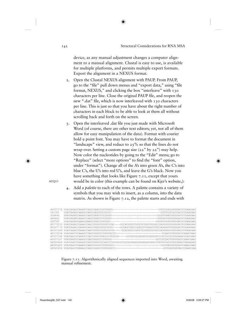
142 Structural Considerations for RNA MSA
device, as any manual adjustment changes a computer align-ment to a manual alignment. Clustal is easy to use, is available for multiple platforms, and permits multiple export formats. Export the alignment in a NEXUS format.
2. Open the Clustal NEXUS alignment with PAUP. From PAUP, go to the “fi le” pull down menus and “export data,” using “fi le format, NEXUS,” and clicking the box “interleave” with 130 characters per line. Close the original PAUP fi le, and reopen the new “.dat” fi le, which is now interleaved with 130 characters per line. This is just so that you have about the right number of characters in each block to be able to look at them all without scrolling back and forth on the screen.
3. Open the interleaved .dat fi le you just made with Microsoft Word (of course, there are other text editors; yet, not all of them allow for easy manipulation of the data). Format with courier bold 9 point font. You may have to format the document in “landscape” view, and reduce to 25% so that the lines do not wrap over. Setting a custom page size (22” by 22”) may help. Now color the nucleotides by going to the “Edit” menu; go to “Replace” (select “more options” to fi nd the “font” option, under “format”). Change all of the A’s into green A’s, the C’s into blue C’s, the U’s into red U’s, and leave the G’s black. Now you have something that looks like Figure 7.11, except that yours would be in color (this example can be found on Kjer’s website,):
4. Add a palette to each of the rows. A palette contains a variety of symbols that you may wish to insert, as a column, into the data matrix. As shown in Figure 7.12, the palette starts and ends with
AY037172 UUAUUAGAUCAAAGCCAAUCGAACUUUCGGGUU-------------------------------CGUUUUAUUGGUGACUCUGAAUAACU61301 UUAUUAGAUCAAAGCCAAUCGAGUUUCGGCUC---------------------------------GUUUUGUUGGUGACUCUGAAUAACZ36893 UUAUUAGAUCAAAGCCAAUCGAACUCUCGGGU-------------------------------UCGUUUAAUUGGUGACUCUGAAUAACX89485 UUAUUAGAUCAAAGCCAAUCGGACUCUCGGGU-------------------------------UCGUAUUGUUGGUGACUCUGAAUAACZ26765 UUAUUAGAUCAAAGCAAAUCGGACCUUCGGG-------------------------------UUCGUUUUGUUGGUGACUCUGAAUAACAF173233 UUAUUAGACCGAAACCAACCUGGUCGUGUCUCAC----GGCACGGUCCGGUCUCUGGCUUUGCCCAGGGGUUUGGUGACUCUGAAUAACAY037170 UUAUUAGACCGAAAUCAACCUGGUCGUUCGCUU-----GCGAGCGGUCCGGUCUCUGGAUCUUCCAGGGGUUUGGUGACUCUGAAUAACAY037169 UUAUUAGACCGAAACCAACCUGGUCGUGUCUCUG-----GCACGGUCCGGUCUCUGGCUUUGUCCAGGGGUUUGGUGACUCUGAAUAACAF173234 UUAUUAGCUCAAAGCCGAUCGGGUCCUUGUGGCCC-------------------------------GCAACUUGGUGACUCAAACGAACAY037168 UUAUUAGCUCAAAGCCGACCGGGCUUAGCCCGCGCUU-----CCGUUCGCGGUGCGCGGGCGGCCCGCCUCUCGGUGAAACGGACGAACAY037167 UUAUUAGUUCAAAGCCGAUCGGGUCCUUUGUG------------------------------GCCCGCUACUUGGUGACUCAAACGAACAF005456 UUAUUAGCUCAAAGCCGACCGGGCUUCAACCCUUCGUCCCCUCGCGGGGCGUUGGGGCGGCCCGUUUCCACUCGGCGAAUCGAAAGAACAF005455 UUAUUAGCUUAAAGCCAAUCGGGUCCUUGUGGCC-------------------------------CGCUUAUUGGUGACUCAAACGAACAF005454 UUAUUAGCUUAAAGCCAAUCGGGUCCUUGUGGCCC--------------------------------GCUUAUUGGUGACUCAAACGAA
Figure 7.11. Algorithmically aligned sequences imported into Word, awaiting manual refi nement.
AUQ13
Rosenberg08_C07.indd 142Rosenberg08_C07.indd 142 9/30/08 5:09:27 PM9/30/08 5:09:27 PM
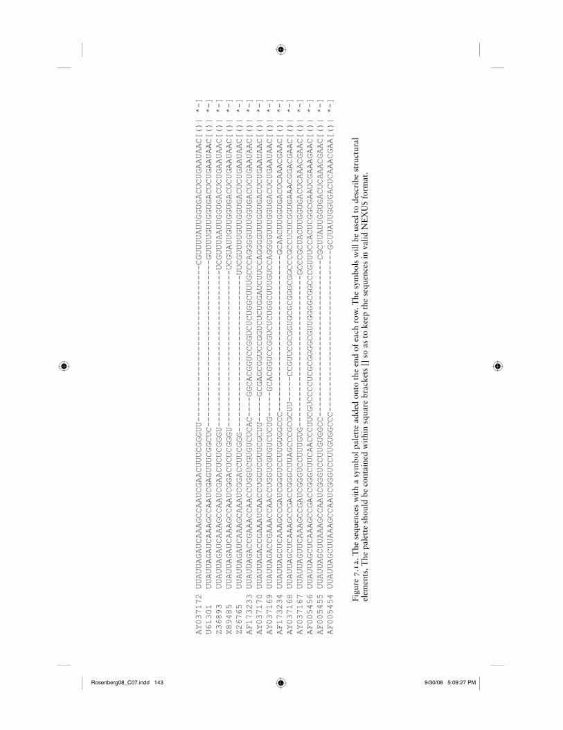
AY037172 UUAUUAGAUCAAAGCCAAUCGAACUUUCGGGUU-------------------------------CGUUUUAUUGGUGACUCUGAAUAAC[()| *-]
U61301 UUAUUAGAUCAAAGCCAAUCGAGUUUCGGCUC---------------------------------GUUUUGUUGGUGACUCUGAAUAAC[()| *-]
Z36893 UUAUUAGAUCAAAGCCAAUCGAACUCUCGGGU-------------------------------UCGUUUAAUUGGUGACUCUGAAUAAC[()| *-]
X89485 UUAUUAGAUCAAAGCCAAUCGGACUCUCGGGU-------------------------------UCGUAUUGUUGGUGACUCUGAAUAAC[()| *-]
Z26765 UUAUUAGAUCAAAGCAAAUCGGACCUUCGGG-------------------------------UUCGUUUUGUUGGUGACUCUGAAUAAC[()| *-]
AF173233 UUAUUAGACCGAAACCAACCUGGUCGUGUCUCAC----GGCACGGUCCGGUCUCUGGCUUUGCCCAGGGGUUUGGUGACUCUGAAUAAC[()| *-]
AY037170 UUAUUAGACCGAAAUCAACCUGGUCGUUCGCUU-----GCGAGCGGUCCGGUCUCUGGAUCUUCCAGGGGUUUGGUGACUCUGAAUAAC[()| *-]
AY037169 UUAUUAGACCGAAACCAACCUGGUCGUGUCUCUG-----GCACGGUCCGGUCUCUGGCUUUGUCCAGGGGUUUGGUGACUCUGAAUAAC[()| *-]
AF173234 UUAUUAGCUCAAAGCCGAUCGGGUCCUUGUGGCCC-------------------------------GCAACUUGGUGACUCAAACGAAC[()| *-]
AY037168 UUAUUAGCUCAAAGCCGACCGGGCUUAGCCCGCGCUU-----CCGUUCGCGGUGCGCGGGCGGCCCGCCUCUCGGUGAAACGGACGAAC[()| *-]
AY037167 UUAUUAGUUCAAAGCCGAUCGGGUCCUUUGUG------------------------------GCCCGCUACUUGGUGACUCAAACGAAC[()| *-]
AF005456 UUAUUAGCUCAAAGCCGACCGGGCUUCAACCCUUCGUCCCCUCGCGGGGCGUUGGGGCGGCCCGUUUCCACUCGGCGAAUCGAAAGAAC[()| *-]
AF005455 UUAUUAGCUUAAAGCCAAUCGGGUCCUUGUGGCC-------------------------------CGCUUAUUGGUGACUCAAACGAAC[()| *-]
AF005454 UUAUUAGCUUAAAGCCAAUCGGGUCCUUGUGGCCC--------------------------------GCUUAUUGGUGACUCAAACGAA[()| *-]
Figu
re 7
.12.
The
seq
uenc
es w
ith
a sy
mbo
l pal
ette
add
ed o
nto
the
end
of e
ach
row
. The
sym
bols
will
be
used
to
desc
ribe
str
uctu
ral
elem
ents
. The
pal
ette
sho
uld
be c
onta
ined
wit
hin
squa
re b
rack
ets
[] s
o as
to
keep
the
seq
uenc
es in
val
id N
EX
US
form
at.
Rosenberg08_C07.indd 143Rosenberg08_C07.indd 143 9/30/08 5:09:27 PM9/30/08 5:09:27 PM
144 Structural Considerations for RNA MSA
brackets, so that NEXUS will ignore the contents after they are eventually reimported into PAUP.
5. Go to Gutell’s (http://www.rna.ccbb.utexas.edu) or Gillespie’s website and download the most recent secondary structure diagram.
6. Microsoft Word permits three essential things you need to be able to do. First, you want to see colors. Second, you must be able to move columns. To move columns in Word, you simply depress the “option” key as you drag down a column with the mouse. Finally, underlines are essential (more about them in step 9). So the next step is to fi nd a stem from a structural model, and paste in the structural symbols from Kjer (1995) to indicate the putative boundaries of the stems. (Note: since 1995, I have replaced the bracket symbols with the “|” symbol to indicate long range stems, because the brackets have meaning in NEXUS that I had not considered in 1995.)
7. Apply structural symbols as in Kjer (1995) to the reference sequence, and fi t them, one by one, onto each of the other sequences. Attempt to subdivide long single-stranded regions by looking for covariation, as in Kjer (1995). As a fi rst pass, assume the structural model you have is correct, but if the data contradict it, then do what the data tell you. Structural models are inferred from comparative evidence, which is exactly what you have before you for a more specifi c set of taxa. These struc-tures may evolve. If you see that your model does not fi t your taxa, then alter it to a model that is supported by the evidence presented by the sequences. The signal in these regions comes from universal and covariable inferred hydrogen bonds (com-pensatory base changes). If all of the taxa can bond in a thermo-dynamically stable stem that is supported by compensatory base changes, and would also be unlikely to exist by chance, then this stem should be inferred and used in an alignment. You may propose modifi cations to structural models this way. It is not your task to construct a perfect secondary structural model, but, rather, to use the structure to infer homology. A portion of the stem for which the structure is ambiguous from the data cannot be used to defi ne homology beyond what you can infer from the nucleotides (primary structure). So you should freely contract stems to the minimum common supported size, and let others
AUQ14
Rosenberg08_C07.indd 144Rosenberg08_C07.indd 144 9/30/08 5:09:27 PM9/30/08 5:09:27 PM
Structural Considerations for RNA MSA 145
whose primary goals are to develop structural models worry about the differences.
8. Consult Hickson et al. (1996) and “Phylogenetic conservation superimposed onto the E. coli SSU rRNA” on Gutell’s website for conserved motifs.
9. Pasting the structural symbols provides only an initial rough hypothesis of base pairing. The next step is to confi rm the hydrogen bonds. Since this is an iterative process, you MUST be able to trace what you have looked at, and differentiate those regions from the regions you have not yet fi nished. One way to do this is with underlines. Underlines indicate confi rmed hydrogen bonds. They mean that you have looked at those individual nucleotides, and their partners, and a Watson–Crick, or G-U, base pair is possible. Laziness is the biggest prob-lem at this point, because it is easy to drag entire columns of nucleotides, and simply underline them all without checking. A sloppy alignment is full of non-Watson–Crick pairs that are mistakenly underlined. Note in Figure 7.13 the bulge indicated by the lack of underlines in Z26765 GCAAA...UUGGU. If you cannot trust the underlines, you cannot trust the alignment. This is why we do not use some of the fancier phylogenetic data editors—because they do not offer the opportunity to visualize individual hydrogen bonds (or if they do, Kjer did not know). There may be a better way to do this. But any system must have confi rmation of bonding at each site, as opposed to a mask applied to the top sequence.
10. Line up the stems. If the stems do not line up because there are alternative lengths, slippage, or a lack of structural conserva-tion, pull back on the stems, and consider them unaligned. Put an empty space to mark the unaligned regions, as above. Use empty spaces to help you break up the alignment, so that you can get a better look at it. Think carefully about data exclusion. For example, can you justify aligning the above UUUUG with CAAC? If not, then eliminate this region, and code it as you see fi t with some other method. The structure will defi ne the aligned regions, and delimit the unaligned regions. If there is no length variation in the single-stranded region, keep it in, as in the region below “V2”: AGAUCAAA. If there is length variation, without conserved nucleotide motifs, throw it out, put it into INAASE,
Rosenberg08_C07.indd 145Rosenberg08_C07.indd 145 9/30/08 5:09:27 PM9/30/08 5:09:27 PM
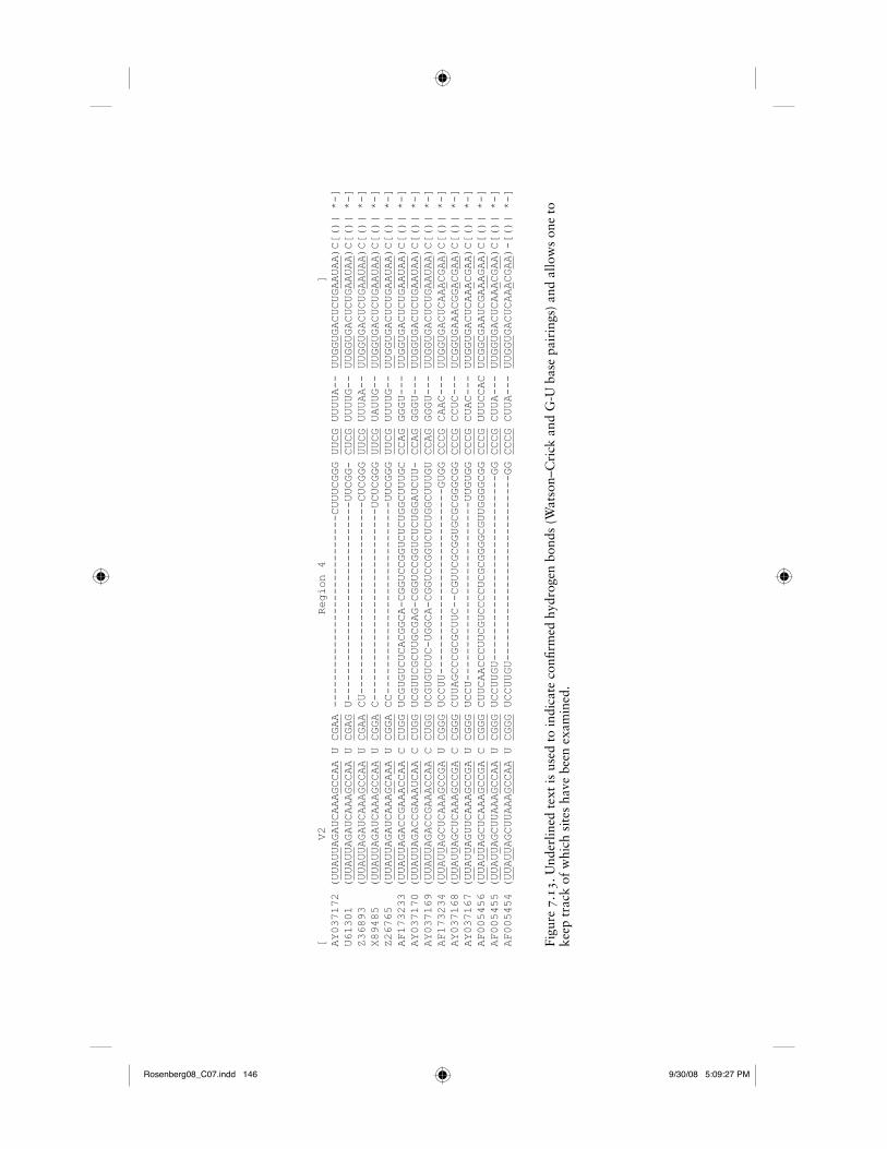
[ V2 Region 4 ]
AY037172 (UUAUUAGAUCAAAGCCAA U CGAA -----------------------------CUUUCGGG UUCG UUUUA-- UUGGUGACUCUGAAUAA)C[()| *-]
U61301 (UUAUUAGAUCAAAGCCAA U CGAG U------------------------------UUCGG- CUCG UUUUG-- UUGGUGACUCUGAAUAA)C[()| *-]
Z36893 (UUAUUAGAUCAAAGCCAA U CGAA CU-----------------------------CUCGGG UUCG UUUAA-- UUGGUGACUCUGAAUAA)C[()| *-]
X89485 (UUAUUAGAUCAAAGCCAA U CGGA C-----------------------------UCUCGGG UUCG UAUUG-- UUGGUGACUCUGAAUAA)C[()| *-]
Z26765 (UUAUUAGAUCAAAGCAAA U CGGA CC-----------------------------UUCGGG UUCG UUUUG-- UUGGUGACUCUGAAUAA)C[()| *-]
AF173233 (UUAUUAGACCGAAACCAA C CUGG UCGUGUCUCACGGCA-CGGUCCGGUCUCUGGCUUUGC CCAG GGGU--- UUGGUGACUCUGAAUAA)C[()| *-]
AY037170 (UUAUUAGACCGAAAUCAA C CUGG UCGUUCGCUUGCGAG-CGGUCCGGUCUCUGGAUCUU- CCAG GGGU--- UUGGUGACUCUGAAUAA)C[()| *-]
AY037169 (UUAUUAGACCGAAACCAA C CUGG UCGUGUCUC-UGGCA-CGGUCCGGUCUCUGGCUUUGU CCAG GGGU--- UUGGUGACUCUGAAUAA)C[()| *-]
AF173234 (UUAUUAGCUCAAAGCCGA U CGGG UCCUU----------------------------GUGG CCCG CAAC--- UUGGUGACUCAAACGAA)C[()| *-]
AY037168 (UUAUUAGCUCAAAGCCGA C CGGG CUUAGCCCGCGCUUC--CGUUCGCGGUGCGCGGGCGG CCCG CCUC--- UCGGUGAAACGGACGAA)C[()| *-]
AY037167 (UUAUUAGUUCAAAGCCGA U CGGG UCCU---------------------------UUGUGG CCCG CUAC--- UUGGUGACUCAAACGAA)C[()| *-]
AF005456 (UUAUUAGCUCAAAGCCGA C CGGG CUUCAACCCUUCGUCCCCUCGCGGGGCGUUGGGGCGG CCCG UUUCCAC UCGGCGAAUCGAAAGAA)C[()| *-]
AF005455 (UUAUUAGCUUAAAGCCAA U CGGG UCCUUGU----------------------------GG CCCG CUUA--- UUGGUGACUCAAACGAA)C[()| *-]
AF005454 (UUAUUAGCUUAAAGCCAA U CGGG UCCUUGU----------------------------GG CCCG CUUA--- UUGGUGACUCAAACGAA)-[()| *-]
Figu
re 7
.13.
Und
erlin
ed t
ext
is u
sed
to in
dica
te c
onfi r
med
hyd
roge
n bo
nds
(Wat
son–
Cri
ck a
nd G
-U b
ase
pair
ings
) an
d al
low
s on
e to
ke
ep t
rack
of
whi
ch s
ites
hav
e be
en e
xam
ined
.
Rosenberg08_C07.indd 146Rosenberg08_C07.indd 146 9/30/08 5:09:27 PM9/30/08 5:09:27 PM
Structural Considerations for RNA MSA 147
or try some iterative tree-based computer alignment on these regions.
11. Think about dots. When applied to sequences to indicate identity with a reference sequence (on top in Figure 7.14), they help you to visualize compensatory base changes, as well as synapo-morphies. They will also make misalignments stand out so that you can see them. You can insert them by moving a section into MacClade, and selecting the “matchar” option, but in doing so, you would lose your structural symbols.
12. Defi ne regions of ambiguous alignment. A candidate for a region of sequence that may be considered as “ambiguously aligned” is initially any region containing length variation among taxa. Objectively subdividing this assignment becomes the more important task because the initial defi nition applies to the whole sequence. There are three types of information that help to designate regions into aligned and ambiguously aligned classes. First, an ambiguously aligned region is any region containing length variation among taxa that is fl anked by hydrogen-bonded stems, in which there is more than one equally plausible alignment. This assignment alone will subdivide the whole gene into multiple fragments. Once the secondary structure has defi ned the boundaries of ambiguity, additional information comes from the nucleotides. Attempt to manually align the region. Consult both Gutell and Hickson et al. for conserved motifs, and if all taxa have them, align the conserved motifs together to further subdivide the region. Ask yourself if a panel of judges were to look at every gap in your alignment, whether or not you could defend your deci-sions to the point where no other placement would be equally parsimonious. Consider transitions to be more likely than transversions, and also, make consistent decisions about how heavily to consider one or a few aberrant taxa in an otherwise length-homogeneous region. Decide the degree of nucleotide similarity among taxa that is required to expand into the regions defi ned by the fl anking hydrogen bonds. Remember, each decision you make is a hypothesis of homology that can be reviewed and overturned. Therefore, you do not need to be perfect, because if you publish your hypotheses, they can be repeated and or contested.
Rosenberg08_C07.indd 147Rosenberg08_C07.indd 147 9/30/08 5:09:28 PM9/30/08 5:09:28 PM

Figu
re 7
.14.
The
use
of
dots
to
indi
cate
iden
tity
wit
h a
refe
renc
e se
quen
ce c
an e
ase
the
iden
tifi c
atio
n of
com
pens
ator
y ba
se c
hang
es,
as w
ell a
s sy
napo
mor
phie
s.
[ V2 Region 4 ]
AY037172 (UUAUUAGAUCAAAGCCAA U CGAA -----------------------------CUUUCGGG UUCG UUUUA-- UUGGUGACUCUGAAUAA)C[()| *-]
U61301 (.................. . ...G U------------------------------UUCGG- C... UUUUG-- ...G.............).[()| *-]
Z36893 (.................. . .... CU-----------------------------CUCGGG .... UUUAA-- .................).[()| *-]
X89485 (.................. . ..G. C-----------------------------UCUCGGG .... UAUUG-- .................).[()| *-]
Z26765 (...............A.. . ..G. CC-----------------------------UUCGGG .... UUUUG-- .................).[()| *-]
AF173233 (........C.G..A.... C .UGG UCGUGUCUCACGGCA-CGGUCCGGUCUCUGGCUUUGC CCA. GGGU--- .................).[()| *-]
AY037170 (........C.G..AU... C .UGG UCGUUCGCUUGCGAG-CGGUCCGGUCUCUGGAUCUU- CCA. GGGU--- .................).[()| *-]
AY037169 (........C.G..A.... C .UGG UCGUGUCUC-UGGCA-CGGUCCGGUCUCUGGCUUUGU CCA. GGGU--- .................).[()| *-]
AF173234 (.......C........G. . ..GG UCCUU----------------------------GUGG CC.. CAAC--- ..........AA.CG..).[()| *-]
AY037168 (.......C........G. C ..GG CUUAGCCCGCGCUUC--CGUUCGCGGUGCGCGGGCGG CC.. CCUC--- .C.....AA.G..CG..).[()| *-]
AY037167 (.......U........G. . ..GG UCCU---------------------------UUGUGG CC.. CUAC--- ..........AA.CG..).[()| *-]
AF005456 (.......C........G. C ..GG CUUCAACCCUUCGUCCCCUCGCGGGGCGUUGGGGCGG CC.. UUUCCAC .C..C..A..GA..G..).[()| *-]
AF005455 (.......C.U........ . ..GG UCCUUGU----------------------------GG CC.. CUUA--- ..........AA.CG..).[()| *-]
AF005454 (.......C.U........ . ..GG UCCUUGU----------------------------GG CC.. CUUA--- ..........AA.CG..)-[()| *-]
Rosenberg08_C07.indd 148Rosenberg08_C07.indd 148 9/30/08 5:09:28 PM9/30/08 5:09:28 PM
Structural Considerations for RNA MSA 149
13. Once you have fi nished the alignment in Word, import the whole thing back into PAUP, and use the “Replace” option in the Edit menu to change all the parentheses, and lines “(“ , ”)” and “ | ” into blank spaces. The NEXUS fi le should be an exact match to the Word fi le, except that it will lack color, and the structural symbols.
Rosenberg08_C07.indd 149Rosenberg08_C07.indd 149 9/30/08 5:09:28 PM9/30/08 5:09:28 PM

AUQ1: (Differentiation of Molecules, 1st paragraph) Please supply reference entry for Cate et al. 1999.
AUQ2: (Compositional Bias Presents a Severe Challenge, 1st paragraph) Please supply reference entry for Brooks and McLennan 1994.
AUQ3: (Compositional Bias Presents a Severe Challenge, 1st paragraph) Please supply reference entry for Lanyon 1988.
AUQ4: (Compositional Bias Presents a Severe Challenge, 1st paragraph) Please supply reference entry for Mishler et al. 1988.
AUQ5: (Gaps Are Not Uniformly Distributed, 3rd paragraph) Suggest defi ne “ILD”AUQ6: (Long Inserts/Deletions, 1st paragraph) Is “nts” an abbreviation for nucleotides? If so,
probably better to write out the wordAUQ7: (Are Structural Inferences Justifi ed?, last line) Would “taxa” in both places be better as
“taxon”?AUQ8: (An Example of Accuracy and Repeatability, 2nd paragraph) Please supply reference entry
for Amrine-Madsen et al. 2003.AUQ9: (An Example of Accuracy and Repeatability, 2nd paragraph) Please supply reference entry
for Delsuc et al. 2002.AUQ10: (An Example of Accuracy and Repeatability, 2nd paragraph) Please supply reference entry
for Waddell and Shelley 2003.AUQ11: (Terminology, 1st paragraph) Please provide reference entries for the “early works of Gutell,
Noller, and Woese.”AUQ12: (Terminology, 1st paragraph) “a single bulge” correct?AUQ13: (Appendix, item 3) Please provide the URL for Kjer’s website.AUQ14: (Appendix, item 5) Please provide the URL for Gillespie’s website.AUQ15: (Figure 7.10 caption) Please supply reference entries for Kjer, Ober, and Gillespie.
Rosenberg08_C07.indd 150Rosenberg08_C07.indd 150 9/30/08 5:09:28 PM9/30/08 5:09:28 PM