Structure, Volume 25

Supplemental Information

Structural Analysis of Multi-component Amyloid

Systems by Chemometric SAXS

Data Decomposition

Fátima Herranz-Trillo, Minna Groenning, Andreas van Maarschalkerweerd, RomàTauler, Bente Vestergaard, and Pau Bernadó

S1

SUPPLEMENTARY INFORMATION

Structural Analysis of Multicomponent Amyloid Systems by Chemometric SAXS Data Decomposition

Fátima Herranz-Trillo,a,b Minna Groenning,b Andreas van Maarschalkerweerd,b Romà Tauler,c Bente Vestergaard, b,* and Pau Bernadóa,*

Afiliations: a Centre de Biochimie Structurale. INSERM U1054, CNRS UMR 5048, Université de Montpellier. 29, rue de Navacelles, 34090-Montpellier, France. b Department of Pharmacy and Department of Drug Design and Pharmacology, University of Copenhagen, Universitetsparken 2, 2100 Copenhagen, Denmark. c Environmental Chemometrics Group, Department of Environmental Chemistry, Institute of Environmental Assessment and Water Diagnostic (IDAEA-CSIC), Barcelona, Spain.

*Authors to whom correspondence should be addressed: Pau Bernadó (pau.bernado@cbs.cnrs.fr) and Bente Vestergaard (bente.vestergaard@sund.ku.dk)

S2

Multivariate Curve Resolution Alternating Least Squares (MCR-ALS) method

Multivariate Curve Resolution (MCR) is a powerful tool for advanced multivariate data analysis. It may

be used in the decomposition of any kind of experimental data, organized as a single data matrix or in

multiple data matrices when multiple experiments are analyzed simultaneously. The basic assumption of

MCR is that measured data variance may be decomposed as the weighted sum of individual

contributions (mixture) coming from the different coexistent components, each one of them defined by a

set of profiles corresponding to each technique applied and weighted according to their composition in

the analyzed mixture.

The bilinear model of MCR is described by the matrix Equation:

D = CST + R (Equation S1)

where the dimensions of the matrices are: D(I,J), C(I,N), ST (N,J) and R(I,J); being I the number of

rows in data matrix D (e,g. the number of spectra measured for instance at different times); J the number

of columns in data matrix D (e.g. the number of wavelengths or momentum transfer points); and N the

number of components (chemical species contributing to the spectroscopic signal). C matrix describes

the composition contributions of the N components (concentration profiles of the different components

at the different reaction times). ST

is the matrix describing the instrumental responses (spectra) of these

N components (pure spectra profiles). Due to unavoidable experimental (noise, etc.) and modeling

uncertainties this matrix decomposition is not perfect, and the differences between the measured data

and their decomposition are collected in a matrix R of residuals. Therefore, the problem to solve in

multivariate curve resolution may be mathematically stated in the following way: given the data matrix

D find: 1) N, the number of chemical components or species causing the observed data variance, D; 2)

find the concentration profiles of these components in matrix C; and 3) find the pure response or spectra

profiles of these components in matrix ST. Stated in this way, and without any further constraint, there is

not a unique set of matrices C and ST that solve Equation S1. In fact there is an infinite number of

mathematically equivalent solutions of C and ST, which multiplied with each other, give the same result

D* = CST. The bilinear decomposition described by Equation S1 is ambiguous if no additional

information is provided, or in other words, there is rotational and scale freedom in the solutions of

Equation S1. This problem is often called in the literature the factor analysis ambiguity problem.

(Malinowski, (2002)) Fortunately, it is usually possible to reduce considerably the number of possible

solutions (and consequently the range of solutions for C and ST matrices) by introducing constraints

derived from the physical nature of the system and/or from prior knowledge of the problem under study.

S3

Among multivariate curve resolution methods, the one based on Alternating Least Squares (MCR-ALS,)

has become very popular. (Tauler, (1995); Tauler, Smilde & Kowalski, (1995); de Juan & Tauler,

(2003); Jaumot et al., (2005); Navea, Tauler & de Juan, (2006)) The MCR-ALS strategy consists of the

following steps:

I. Determination of the number of significant components (N) present in the matrix D using

Singular Value Decomposition (SVD) or Principal Component Analysis (PCA). The analysis

of the size of the eigenvalues and shape of the eigenvectors derived from the data matrix D

identify the number of (relevant) chemical components or species present in the analyzed

mixtures. Unavoidable experimental errors and noise are associated to non-significant (non-

relevant) species.

II. Generation of initial estimates of concentration or spectra profiles. Once the number of

components, N, has been determined, an initial estimate of their concentration or spectra

profiles can be obtained by different methods, based for instance on the selection of the

purest variables (Maeder, (1987); Windig & Guilment, (1991)) in the experimental data

matrix D. Steps I and II can also be done using previous knowledge of the chemical problem

under investigation to propose directly the number of components and the initial estimates.

III. Resolution of equation S1 by the alternating least squares (ALS) algorithm. In the

unconstrained case, this involves two steps:

C = DS(STS)-1 (Equation S2)

ST = (CTC)-1CTD (Equation S3)

Constraints can be incorporated into the optimization process in order to render the solution chemically

meaningful. A constraint is defined as a particular characteristic of chemical or mathematical nature that

the spectra of the pure components or the concentration profiles must obey. Usually, non-negativity can

always be applied to the concentration profiles and also to multiple types of spectra (not for derivative

and difference spectra or for Circular Dichroism). Unimodality constraint forces the presence of a single

maximum per profile, which in some cases can be applied to concentrations profiles (e.g reaction and

chromatographic systems). Closure constraint is related with mass balance, and it can be introduced for

the concentration C matrix. Local rank-based or selectivity constraints can be applied when one or

several species are known not to be present in a particular region or window of the dataset (in both the

S4

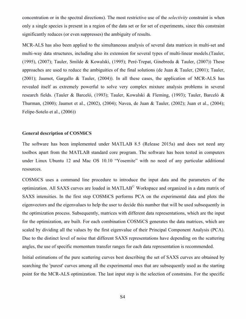
concentration or in the spectral directions). The most restrictive use of the selectivity constraint is when

only a single species is present in a region of the data set or for set of experiments, since this constraint

significantly reduces (or even suppresses) the ambiguity of results.

MCR-ALS has also been applied to the simultaneous analysis of several data matrices in multi-set and

multi-way data structures, including also its extension for several types of multi-linear models.(Tauler,

(1995), (2007); Tauler, Smilde & Kowalski, (1995); Peré-Trepat, Ginebreda & Tauler, (2007)) These

approaches are used to reduce the ambiguities of the final solutions (de Juan & Tauler, (2001); Tauler,

(2001); Jaumot, Gargallo & Tauler, (2004)). In all these cases, the application of MCR-ALS has

revealed itself as extremely powerful to solve very complex mixture analysis problems in several

research fields. (Tauler & Barceló, (1993); Tauler, Kowalski & Fleming, (1993); Tauler, Barceló &

Thurman, (2000); Jaumot et al., (2002), (2004); Navea, de Juan & Tauler, (2002); Juan et al., (2004);

Felipe-Sotelo et al., (2006))

General description of COSMiCS

The software has been implemented under MATLAB 8.5 (Release 2015a) and does not need any

toolbox apart from the MATLAB standard core program. The software has been tested in computers

under Linux Ubuntu 12 and Mac OS 10.10 “Yosemite” with no need of any particular additional

resources.

COSMiCS uses a command line procedure to introduce the input data and the parameters of the

optimization. All SAXS curves are loaded in MATLAB© Workspace and organized in a data matrix of

SAXS intensities. In the first step COSMiCS performs PCA on the experimental data and plots the

eigenvectors and the eigenvalues to help the user to decide this number that will be used subsequently in

the optimization process. Subsequently, matrices with different data representations, which are the input

for the optimization, are built. For each combination COSMiCS generates the data matrices, which are

scaled by dividing all the values by the first eigenvalue of their Principal Component Analysis (PCA).

Due to the distinct level of noise that different SAXS representations have depending on the scattering

angles, the use of specific momentum transfer ranges for each data representation is recommended.

Initial estimations of the pure scattering curves best describing the set of SAXS curves are obtained by

searching the 'purest' curves among all the experimental ones that are subsequently used as the starting

point for the MCR-ALS optimization. The last input step is the selection of constrains. For the specific

S5

case of fibrillating proteins the constrains used in COSMiCS were:

- Non-negativity. This constraint forces both concentrations and scattering intensities to have

positive values. This is achieved using the fast non-negativity least squares algorithm (fast

NNLS or FNNLS), which is a modification of the standard algorithm NNLS (Bro & De Jong,

(1997)). This constraint has been applied to both concentrations and spectra. In particular, in all

the steps of the ALS algorithm the values of the populations and spectra are evaluated and

constrained not to be negative. Since the ‘true’ solution is non-negative, the application of this

constraint drives the optimization to this true solution and avoids negative solutions fitting

equally well the data in a least squares sense.

- Closure. This constraint forces the system to be closed. In other words, it forces the sum of the

molar fractions of the different species of the mixture to be equal to 1.0 in all points of the

dataset (de Juan & Tauler, (2003); Jaumot et al., (2005)). The concentration of the species i is

updated during every ALS step, using the expression:

𝐶!,!′ =𝐶!,!𝐶!,!!

!!!

where Ci,k’ is the updated concentration value, Ci,k is the currently ALS calculated concentration

value, and the denominator corresponds to the sum of the concentration of all coexisting species

(k=1,N, and i refers to the considered spectrum/sample). This constraint is applied at each step of

the algorithm.

- Selectivity. This constraint is implemented in COSMiCS but it has not been used in the present

study, as the presence of a single species was not guaranteed in any of the measured time-points.

- Unimodality. This constraint has not been implemented in COSMiCS due to the stochasticity of

the onset of the fibrillation reaction which precludes the identification of a single maximum of

the concentration profile.”

In the present application of COSMiCS, the maximum number of iterations was set to 50, and the

convergence criteria was defined as a 0.1% of change in the standard deviation of the residuals.

Once the input is introduced, the MCR-ALS optimization is performed first for the absolute value

representation of the data, and repeated afterwards for every combination of SAXS representations. For

the cases where several representations of the data were analyzed simultaneously, a row-wise

augmented matrix of spectra was used as input dataset assuming that a single matrix of concentration

profiles is valid for all the simultaneously analyzed datasets.

S6

After each optimization, the COSMiCS procedure back calculates the solution curves and compares

them with the experimental data set to derive individual χi2 values and their averages 〈χi

2〉. A graphical

interface of COSMiCS displays all the optimized curves for each combination. Using the graphical

inspection and 〈χi2〉 values, the user decides which is the combination that has provided the best solution.

After this selection, the program displays the ten curves with the worst χi2 values allowing the user to

remove individual curves from the analysis and to run the complete procedure again. COSMiCS

provides then Δχi2 between both optimizations for each individual curve to confirm the overall benefit

of the curve removal and the improvement of results. This procedure can be repeated until robust and

consistent solutions are obtained.

COSMiCS Flowchart

Proper SAXS-based structural modeling procedures require proper estimations of the error uncertainty

bars for each of the intensity values. The uncertainties on both SAXS curves and concentration profiles

are derived using a Monte Carlo error analysis similar to what was previously used by Svergun and

Pedersen (Svergun & Pedersen, (1994)). To perform this analysis, random noise based on the

S7

experimental uncertainty bars is added to each of the back-calculated curves. This new synthetic dataset

is then submitted to the MCR-ALS optimization. This process is repeated one hundred times using

different values of random noise. The optimized SAXS curves and the concentration profiles for each

Monte Carlo cycle that converge are stored and the standard deviations for the intensities, I(s), and for

the concentrations profiles are calculated.

S8

Generation and COSMiCS analysis of a synthetic SAXS dataset Generation of the Synthetic dataset: We have generated a synthetic SAXS dataset based on the

selecase oligomerization (López-Pelegrín et al., (2014)). Concretely, we designed a monomer-dimer-

tetramer model corresponding to pdb codes 4QHF, 4QHG and 4QHH, respectively. Their theoretical

scattering profiles were computed with CRYSOL (Svergun, Barberato & Koch, (1995)) using the

maximum number of spherical harmonics and maximum order of the Fibonacci’s grid representation.

All other parameters were in default setting. These three curves were scaled in order to have a

monomeric species curve with a forward scattering, I(0), equivalent to the curve of 8.5 mg/ml selecase

concentration from the experimental dataset. A population (kinetic) model that included a Gaussian

population for the dimeric species was generated making sure that the sum of molar fractions for each

time-point was 1.0. The final dataset of curves was calculated for 50 time-points using the synthetic

profiles for the three species and the molar fractions of the kinetic model. Synthetic noise was added to

these curves based on the experimental error estimations of the experimental SAXS curve of selecase at

8.5 mg/ml. Error in successive synthetic curves was increased according to the square root of the ratio

I(0)theo/I(0)exp , where I(0)theo was the forward scattering of each synthetic curve, and I(0)exp is the

forward scattering of the experimental curve of selecase at 8.5 mg/ml. Two independent datasets were

generated: one assuming the experimental noise, and a second one with the double noise. Both datasets

yielded very similar results with the COSMiCS analysis. We are only presenting results of the double

noise dataset (Figure S1A).

COSMiCS analysis: COSMiCS was applied to the synthetic dataset using closure and non-negativity

as constraints (see above). The <χ2> resulting from the different combinations of data representations

are displayed in the table. A very good agreement to the complete dataset is observed for the majority of

combinations. Some combinations including Porod’s representation present larger <χ2>. The resulting

decomposed curve profiles for the three species and their relative populations are in excellent agreement

with the theoretical values used to simulate the data. Importantly, all combinations with <χ2> smaller

than 1.0 present almost equivalent results. In supplementary figure S1 the results of the AH combination

are presented.

S9

Results of the COSMiCS analysis of the synthetic dataset

Representations included

Code Absolute

I(s) Holtzer I(s)*s

Kratky I(s)*s2

Porod I(s)*s4

〈χi2〉

A + 0.95 AH + + 0.93 AK + + 0.93 AP + + 1.24

AHK + + + 0.93 AHP + + + 1.22 AKP + + + 0.95

AHKP + + + + 0.95

Dataset and results from the decomposition of the synthetic data set using COSMiCS: (A) Complete synthetic data set in logarithmic scale. (B) SAXS profiles for the isolated species for the AH combination: monomer (blue), dimer (green) and tetramer (orange) and the original CRYSOL curves superimposed in darker colors. (C) Kinetic model used to create the data set (solid lines) and the concentration profiles derived from COSMiCS (dots), with the same color code as the spectra profiles.

S10

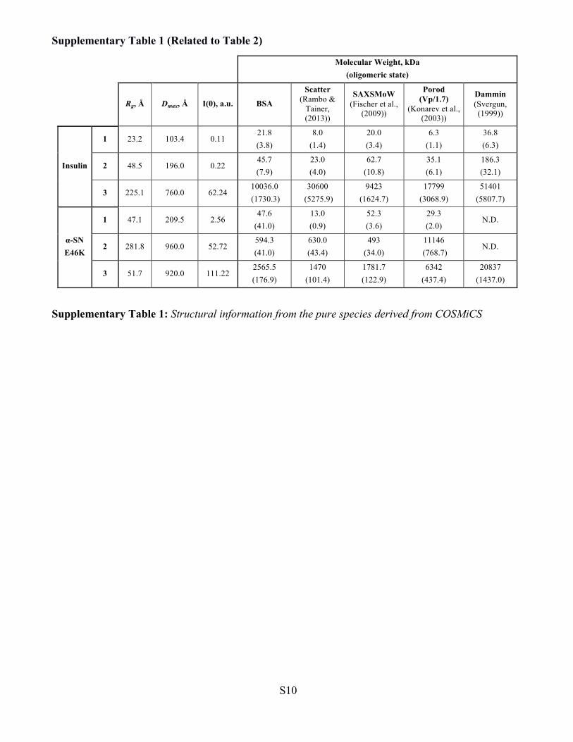
Supplementary Table 1 (Related to Table 2)

Molecular Weight, kDa

(oligomeric state)

Rg, Å Dmax, Å I(0), a.u. BSA

Scatter (Rambo &

Tainer, (2013))

SAXSMoW (Fischer et al.,

(2009))

Porod (Vp/1.7)

(Konarev et al., (2003))

Dammin (Svergun, (1999))

Insulin

1 23.2 103.4 0.11 21.8 (3.8)

8.0 (1.4)

20.0 (3.4)

6.3 (1.1)

36.8 (6.3)

2 48.5 196.0 0.22 45.7 (7.9)

23.0 (4.0)

62.7 (10.8)

35.1 (6.1)

186.3 (32.1)

3 225.1 760.0 62.24 10036.0 (1730.3)

30600 (5275.9)

9423 (1624.7)

17799 (3068.9)

51401 (5807.7)

α-SN E46K

1 47.1 209.5 2.56 47.6

(41.0) 13.0 (0.9)

52.3 (3.6)

29.3 (2.0)

N.D.

2 281.8 960.0 52.72 594.3 (41.0)

630.0 (43.4)

493 (34.0)

11146 (768.7)

N.D.

3 51.7 920.0 111.22 2565.5 (176.9)

1470 (101.4)

1781.7 (122.9)

6342 (437.4)

20837 (1437.0)

Supplementary Table 1: Structural information from the pure species derived from COSMiCS

S11

Supplementary Figure 1 (Related to Figure 1 and 3)

Supplementary Figure 1: SAXS profiles (black dots) showing the evolution of fibrillation of insulin (left) and α-SN E46K (right) and the MCR-ALS fits (red solid lines) (see main text for details). Log-Log representations of Figures 1 and 3 in the main text.

S12

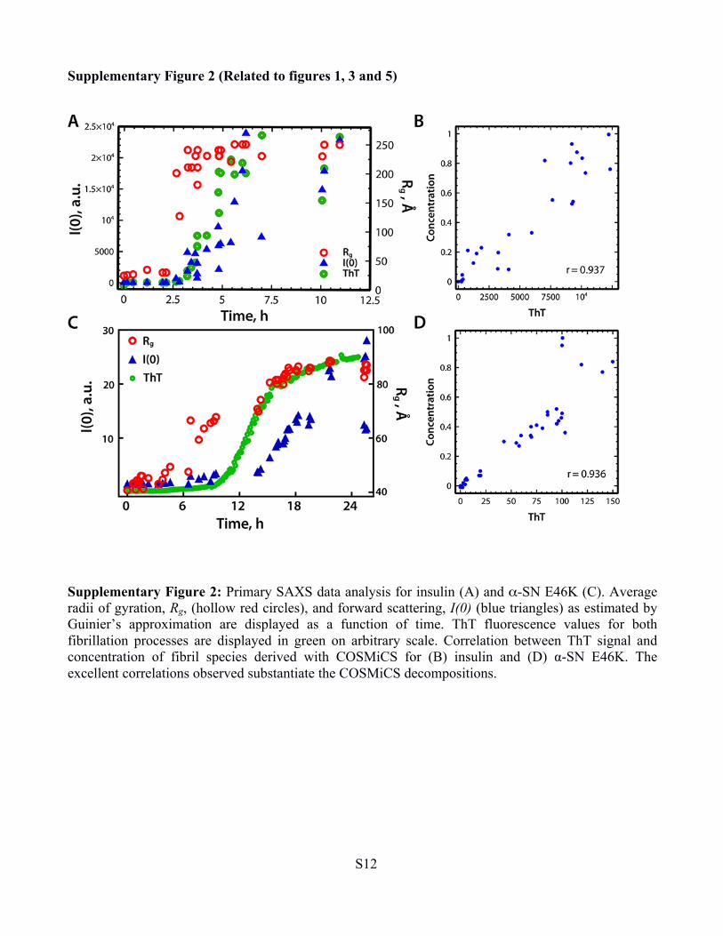
Supplementary Figure 2 (Related to figures 1, 3 and 5)

Supplementary Figure 2: Primary SAXS data analysis for insulin (A) and α-SN E46K (C). Average radii of gyration, Rg, (hollow red circles), and forward scattering, I(0) (blue triangles) as estimated by Guinier’s approximation are displayed as a function of time. ThT fluorescence values for both fibrillation processes are displayed in green on arbitrary scale. Correlation between ThT signal and concentration of fibril species derived with COSMiCS for (B) insulin and (D) α-SN E46K. The excellent correlations observed substantiate the COSMiCS decompositions.

S13

Supplementary Figure 3 (Related to Figures 1 and 3)

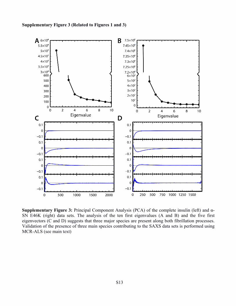
Supplementary Figure 3: Principal Component Analysis (PCA) of the complete insulin (left) and α-SN E46K (right) data sets. The analysis of the ten first eigenvalues (A and B) and the five first eigenvectors (C and D) suggests that three major species are present along both fibrillation processes. Validation of the presence of three main species contributing to the SAXS data sets is performed using MCR-ALS (see main text)

S14

Supplementary Figure 4 (Related to Figure 1)

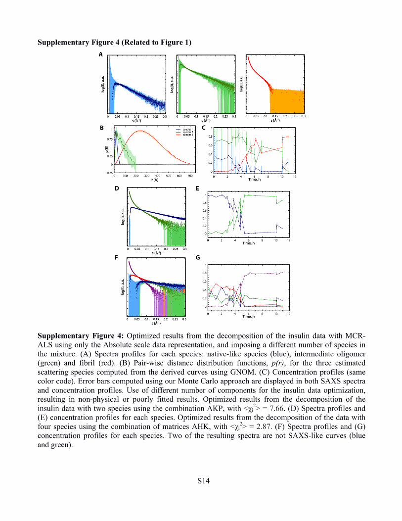
Supplementary Figure 4: Optimized results from the decomposition of the insulin data with MCR-ALS using only the Absolute scale data representation, and imposing a different number of species in the mixture. (A) Spectra profiles for each species: native-like species (blue), intermediate oligomer (green) and fibril (red). (B) Pair-wise distance distribution functions, p(r), for the three estimated scattering species computed from the derived curves using GNOM. (C) Concentration profiles (same color code). Error bars computed using our Monte Carlo approach are displayed in both SAXS spectra and concentration profiles. Use of different number of components for the insulin data optimization, resulting in non-physical or poorly fitted results. Optimized results from the decomposition of the insulin data with two species using the combination AKP, with <χi

2> = 7.66. (D) Spectra profiles and (E) concentration profiles for each species. Optimized results from the decomposition of the data with four species using the combination of matrices AHK, with <χi

2> = 2.87. (F) Spectra profiles and (G) concentration profiles for each species. Two of the resulting spectra are not SAXS-like curves (blue and green).

S15

Supplementary Figure 5 (Related to Figure 1)

Supplementary Figure 5: Representations of the SAXS data measured along the fibrillation of insulin and used in our COSMiCS approach. (A) Absolute values, I(s). (B) Holtzer, I(s)·s. (C) Kratky, I(s)·s2. (D) Porod, I(s)·s4. Different features are observed in the momentum transfer range displayed along the fibrillation process represented with a blue color scale, from light blue (t=0) to dark blue (t=11 h).

S16

Supplementary Figure 6 (Related to Figure 1 and 5)

Supplementary Figure 6: Structural analysis of some of the species derived from the COSMiCS analysis (A) Kratky representation of the monomeric insulin derived from COSMiCS indicating that the isolated monomeric species is partially unfolded. (B) Fitting with CRYSOL of the folded monomeric insulin extracted from pdb 1EV6 to the curve isolated using COSMiCS for the monomeric species (see main text for details) (C) EOM fitting (red curve) of the α−SNE46K curve isolated with COSMiCS (black dots), with a χ2=1.12. (D) The distributions of radii of gyrations for the pool of α−SNE46K conformations (black)) and the EOM selected ones (red). (E) Three orientations of the ab initio structure of the fibril repeating unit of α-SN E46K determined from the decomposed curve with COSMiCS. Average from 20 refined models computed with the program DAMMIN.

S17

Supplementary Figure 7 (Related to Figures 1 and 3)

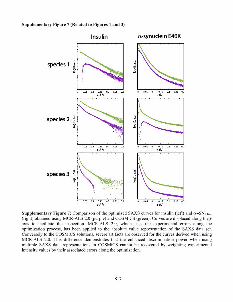
Supplementary Figure 7: Comparison of the optimized SAXS curves for insulin (left) and α−SNE46K (right) obtained using MCR-ALS 2.0 (purple) and COSMiCS (green). Curves are displaced along the y axis to facilitate the inspection. MCR-ALS 2.0, which uses the experimental errors along the optimization process, has been applied to the absolute value representation of the SAXS data set. Conversely to the COSMiCS solutions, severe artifacts are observed for the curves derived when using MCR-ALS 2.0. This difference demonstrates that the enhanced discrimination power when using multiple SAXS data representations in COSMiCS cannot be recovered by weighting experimental intensity values by their associated errors along the optimization.

S18

Supplementary References

Bro, R. & De Jong, S. (1997). A fast non-negativity-constrained least squares algorithm. J. Chemom. 11, 393–401.

Felipe-Sotelo, Gustems, L., Hernandez, I., Terrado, M. & Tauler, R. (2006). Investigation of geographical and temporal distribution of tropospheric ozone in Catalonia (North-East Spain) during the period 2000–2004 using multivariate data analysis methods. Atmos. Environ. 40, 7421–7436.

Fischer, H., de Oliveira Neto, M., Napolitano, H.B., Polikarpov, I. & Craievich, A.F. (2009). Determination of the molecular weight of proteins in solution from a single small-angle X-ray scattering measurement on a relative scale. J. Appl. Crystallogr. 43, 101–109.

Jaumot, J., Escaja, N., Gargallo, R., González, C., Pedroso, E. & Tauler, R. (2002). Multivariate curve resolution: a powerful tool for the analysis of conformational transitions in nucleic acids. Nucleic Acids Res. 30, e92.

Jaumot, J., Gargallo, R. & Tauler, R. (2004). Noise propagation and error estimations in multivariate curve resolution alternating least squares using resampling methods. J. Chemom. 18, 327–340.

Jaumot, J., Marchán, V., Gargallo, R., Grandas, A. & Tauler, R. (2004). Multivariate Curve Resolution Applied to the Analysis and Resolution of Two-Dimensional [ 1 H, 15 N] NMR Reaction Spectra. Anal. Chem. 76, 7094–7101.

Jaumot, J., Gargallo, R., de Juan, A. & Tauler, R. (2005). A graphical user-friendly interface for MCR-ALS: a new tool for multivariate curve resolution in MATLAB. Chemom. Intell. Lab. Syst. 76, 101–110.

Juan, A. de, Tauler, R., Dyson, R., Marcolli, C., Rault, M. & Maeder, M. (2004). Spectroscopic imaging and chemometrics: a powerful combination for global and local sample analysis. TrAC Trends Anal. Chem. 23, 70–79.

de Juan, A. & Tauler, R. (2001). Comparison of three-way resolution methods for non-trilinear chemical data sets. J. Chemom. 15, 749–771.

de Juan, A. & Tauler, R. (2003). Chemometrics applied to unravel multicomponent processes and mixtures. Anal. Chim. Acta. 500, 195–210.

Konarev, P. V., Volkov, V. V., Sokolova, A. V., Koch, M.H.J. & Svergun, D.I. (2003). PRIMUS  : a Windows PC-based system for small-angle scattering data analysis. J. Appl. Crystallogr. 36, 1277–1282.

López-Pelegrín, M., Cerdà-Costa, N., Cintas-Pedrola, A., Herranz-Trillo, F., Bernadó, P., Peinado, J.R., Arolas, J.L. & Gomis-Rüth, F.X. (2014). Multiple Stable Conformations Account for Reversible Concentration-Dependent Oligomerization and Autoinhibition of a Metamorphic Metallopeptidase. Angew. Chemie Int. Ed. 53, 10624–10630.

Maeder, M. (1987). Evolving factor analysis for the resolution of overlapping chromatographic peaks. Anal. Chem. 59, 527–530.

Malinowski, E. (2002). Factor analysis in chemistry. ed. (New York, NY: Wiley-Interscience).

Navea, S., de Juan, A. & Tauler, R. (2002). Detection and resolution of intermediate species in protein

S19

folding processes using fluorescence and circular dichroism spectroscopies and multivariate curve resolution. Anal. Chem. 74, 6031–9.

Navea, S., Tauler, R. & de Juan, A. (2006). Monitoring and Modeling of Protein Processes Using Mass Spectrometry, Circular Dichroism, and Multivariate Curve Resolution Methods. Anal. Chem. 78, 4768–4778.

Peré-Trepat, E., Ginebreda, A. & Tauler, R. (2007). Comparison of different multiway methods for the analysis of geographical metal distributions in fish, sediments and river waters in Catalonia. Chemom. Intell. Lab. Syst. 88, 69–83.

Rambo, R.P. & Tainer, J.A. (2013). Accurate assessment of mass, models and resolution by small-angle scattering. Nature. 496, 477–81.

Svergun, D.I. (1999). Restoring low resolution structure of biological macromolecules from solution scattering using simulated annealing. Biophys. J. 76, 2879–86.

Svergun, D.I. & Pedersen, J.S. (1994). Propagating errors in small-angle scattering data treatment. J. Appl. Crystallogr. 27, 241–248.

Svergun, D.I., Barberato, C. & Koch, M.H.J. (1995). CRYSOL-a program to evaluate X-ray solution scattering of biological macromolecules from atomic coordinates. J. Appl. …. 768–773.

Tauler, R. (1995). Multivariate curve resolution applied to second order data. Chemom. Intell. Lab. Syst. 30, 133–146.

Tauler, R. (2001). Calculation of maximum and minimum band boundaries of feasible solutions for species profiles obtained by multivariate curve resolution. J. Chemom. 15, 627–646.

Tauler, R. (2007). Application of non-linear optimization methods to the estimation of multivariate curve resolution solutions and of their feasible band boundaries in the investigation of two chemical and environmental simulated data sets. Anal. Chim. Acta. 595, 289–98.

Tauler, R. & Barceló, D. (1993). Multivariate curve resolution applied to liquid chromatography—diode array detection. TrAC Trends Anal. Chem. 12, 319–327.

Tauler, R., Kowalski, B. & Fleming, S. (1993). Multivariate curve resolution applied to spectral data from multiple runs of an industrial process. Anal. Chem. 65, 2040–2047.

Tauler, R., Smilde, A.K. & Kowalski, B. (1995). Selectivity, local rank, three‐way data analysis and ambiguity in multivariate curve resolution. J. Chemom. 9, 31–58.

Tauler, R., Barceló, D. & Thurman, E.M. (2000). Multivariate Correlation between Concentrations of Selected Herbicides and Derivatives in Outflows from Selected U.S. Midwestern Reservoirs. Environ. Sci. Technol. 34, 3307–3314.

Windig, W. & Guilment, J. (1991). Interactive self-modeling mixture analysis. Anal. Chem. 63, 1425–1432.