Embed Size (px)
Citation preview

Published: September 16, 2011
r 2011 American Chemical Society 7710 dx.doi.org/10.1021/cr100353t |Chem. Rev. 2011, 111, 7710–7748
REVIEW
pubs.acs.org/CR
Structural Analysis of Macromolecular Assemblies byElectron MicroscopyE. V. Orlova* and H. R. Saibil*
Crystallography and Institute of Structural and Molecular Biology, Birkbeck College, Malet Street, London WC1E 7HX,United Kingdom
CONTENTS
1. Introduction 77111.1. Light and ElectronMicroscopy and Their Impact
in Biology 7711
1.2. EM of Macromolecular Assemblies, Isolated andin Situ 7711
2. EM Imaging 77112.1. Sample Preparation 7711
2.1.1. Negative Staining of IsolatedAssemblies 7712
2.1.2. Cryo EM of Isolated and SubcellularAssemblies 7712
2.1.3. Stabilization of Dynamic Assemblies 77132.1.4. EM Preparation of Cells and Tissues 7713
2.2. Interaction of Electrons with the Specimen 77142.3. Image Formation 7715
2.3.1. Electron Sources 77152.3.2. The Electron Microscope Lens System 77162.3.3. Electron Microscope Aberrations 7716
2.4. Contrast Transfer 77162.4.1. Formation of Projection Images 77172.4.2. Contrast for Thin Samples 7717
2.5. Phase Plates and Energy Filters 77193. Image Recording and Preprocessing 7720
3.1. Electron Detectors 77203.1.1. Photographic Film 77203.1.2. Digitization of Films 77203.1.3. Digital Detectors 7721
3.2. Computer-Controlled Data Collection andParticle Picking 7721
3.3. Tomographic Data Collection 77223.4. Preprocessing of Single-Particle Images 7722
3.4.1. Determination of the CTF 77233.4.2. CTF Correction 77233.4.3. Image Normalization 7724
4. Image Alignment 77244.1. The Cross-Correlation Function 77254.2. Alignment Principles and Strategies 7725
4.2.1. Maximum Likelihood Methods 77274.3. Template Matching in 2D and 3D 77274.4. Alignment in Tomography 7727
4.4.1. Alignment with and without FiducialMarkers 7727
4.4.2. Alignment of Subregions Extracted fromTomograms 7727
5. Statistical Analysis of Images 77285.1. Principal Component Analysis 77285.2. Hierarchical Clustering 77295.3. K-Means Clustering and the Maximum Likeli-
hood Method 77296. Orientation Determination 7729
6.1. Random Conical Tilt 77296.2. Angle Assignment by Common Lines in Reci-
procal Space 7731
6.3. Common Lines in Real Space 77326.4. Projection Matching 77326.5. Molecular Replacement 7732
7. 3D Reconstruction 77337.1. Real-Space Methods 7733
7.1.1. Back Projection 77337.1.2. Filtered Back-Projection or Convolution
Methods 7734
7.1.3. Algebraic Methods 77347.2. Fourier Methods 7736
7.2.1. Fourier Inversion 77367.2.2. Fourier�Bessel Reconstruction 7736
7.3. Distribution of Projections 77377.4. Electron Crystallography 77377.5. Tomographic Reconstruction 7738
8. Evaluation of Reconstruction Quality and Reliability 77398.1. Causes of Resolution Loss 77398.2. Resolution Measures 77398.3. Temperature Factor and Amplitude Scaling
(Sharpening) 77419. Heterogeneity in 2D and 3D 7741
9.1. Sources of Heterogeneity 77419.2. Methods for Computational Sorting of Mixed
Structures 774110. Map Interpretation 7743
10.1. Analysis of Map Features 7743
Received: October 21, 2010
7711 dx.doi.org/10.1021/cr100353t |Chem. Rev. 2011, 111, 7710–7748
Chemical Reviews REVIEW
10.2. Atomic Structure Fitting 774410.3. Biological Implications 7744
Author Information 7744Biographies 7744Acknowledgment 7745References 7745
1. INTRODUCTION
1.1. Light and Electron Microscopy and Their Impact inBiology
To fully understand biological processes from the metabolismof a bacterium to the operation of a human brain, it is necessary toknow the three-dimensional (3D) spatial arrangement anddynamics of the constituent molecules, how they assemble intocomplex molecular machines, and how they form functionalorganelles, cells, and tissues. The methods of X-ray crystal-lography and NMR spectroscopy can provide detailed informa-tion on molecular structure and dynamics. At the cellular level,optical microscopy reveals the spatial distribution and dynamicsof molecules tagged with fluorophores. Electron microscopy(EM) overlaps with these approaches, covering a broad rangefrom atomic to cellular structures. The development of cryogenicmethods has enabled EM imaging to provide snapshots ofbiological molecules and cells trapped in a close to native,hydrated state.1,2
Because of the importance of macromolecular assemblies inthe machinery of living cells and progress in the EM and imageprocessing methods, EM has become a major tool for structuralbiology over themolecular to cellular size range. There have beentremendous advances in understanding the 3D spatial organiza-tion of macromolecules and their assemblies in cells and tissues,due to developments in both optical and electron microscopy. Inlight microscopy, super-resolution and single molecule methodshave pushed the resolution of fluorescence images to ∼50 nm,using the power of molecular biology to fuse molecules ofinterest with fluorescent marker proteins.3 X-ray cryo-tomogra-phy is developing as a method for 3D reconstruction of thicker(10 μm) hydrated samples, with resolution reaching the 15 nmresolution range.4 In EM, major developments in instrumenta-tion and methods have advanced the study of single particles(isolated macromolecular complexes) in vitrified solution as wellas in 3D reconstruction by tomography of irregular objects suchas cells or subcellular structures.1,5�7 Cryo-sectioning can beused to prepare vitrified sections of cells and tissues that wouldotherwise be too thick to image by transmission EM (TEM).8,9
In parallel, software improvements have facilitated 3D struc-ture determination from the low contrast, low signal-to-noiseratio (SNR) images of projected densities provided by TEM ofbiological molecules.10�14 Alignment and classification of imagesin both 2D and 3D are key methods for improving SNR anddetection and sorting of heterogeneity in EM data sets.14 Theresolution of single-particle reconstructions is steadily improvingand has gone beyond 4 Å for some icosahedral viruses and 5.5 Åfor asymmetric complexes such as ribosomes, giving a clear viewof protein secondary structure elements and, in the best cases,resolving the protein or nucleic acid fold.15,16
1.2. EM of Macromolecular Assemblies, Isolated and in SituA variety of molecular assemblies of different shapes, sizes, and
biochemical states can be studied by TEM, provided the sample
thickness is well below 1000 nm. There is a range of sample typestypified by two extreme cases: biochemically purified, isolatedcomplexes (single particles or ordered assemblies such as 2Dcrystals) and unique, individual objects such as tissue sections,cells, or organelles. From preparations of isolated complexes withmany identical single particles present on an EM grid, manyviews of the same molecule can be obtained, so that their 3Dstructure can be calculated. Near-atomic resolution maps werefirst obtained from samples in ordered arrays such as 2D crystalsand helices.17,18 Membrane proteins can be induced to form 2Dcrystals in lipid bilayers, although examples of highly orderedcrystals leading to high-resolution 3D structures are still rare. Ifmembrane-bound complexes are large enough, they can also beprepared as single particles using detergents or in liposomes. Ingeneral, the single-particle approach is widely applicable and hascaught up with the crystallographic one. This approach isapplicable to homogeneous preparations of single particles withany symmetry and molecular masses in the range of 0.5�100 MDa (e.g., viruses, ribosomes) and can reveal fine detailsof the 3D structure.15 The study of single particles by cryo-EM inthe 0.1�0.5 MDa size range still needs great care to avoidproducing false but self-consistent density maps. In addition,the single-particle approach can be used to correct for localdisorder in ordered arrays, improving the yield of structuralinformation. Regarding the quality of this structural information,the resolution of cryo-EM is steadily improving, and comparisonsof cryo-EM results with X-ray crystallography or NMR of thesame molecules indicate that cryo-EM often provides faithfulsnapshots of the native structure in solution. A detailedaccount of the basic principles of imaging and diffractioncan be found in ref 19.
For cells, organelles, and tissue sections, electron tomographyprovides a wealth of 3D information, and methods for harvestingthis information are in an active state of development. Auto-mated tomographic data collection is well established onmodernmicroscopes. A major factor limiting resolution in cryo-electrontomography is radiation damage of the specimen by the electronbeam during acquisition of a tilt series. At the forefront of thisfield are efforts to optimize contrast at low electron dose, in orderto locate and characterize macromolecular complexes withintomograms of cells and tissues. At present, complexes must bewell over 1 MDa to be clearly identifiable in an EM tomographicreconstruction. Examples of important biological structures char-acterized by electron tomography include the nuclear porecomplex20 and the flagellar axoneme.21 For thicker, cellularsamples, X-ray microscopy (tomography) provides informationin the 15�100 nm resolution range, bridging EM tomographyand fluorescence methods.
The above developments have led to a flourishing field enablingmultiscale imaging to link atomic structure to cellular functionand dynamics. In this Review, we aim to cover the theoreticalbackground and technical advances in instrumentation, software,and experimental methods underlying the major developmentsin 3D structure determination of macromolecular assemblies byEM and to review the current state of the art in the field.
2. EM IMAGING
2.1. Sample PreparationElectron imaging is a powerful technique for visualizing 3D
structural details. However, because electrons interact stronglywith matter, the electron path of the microscope must be kept
7712 dx.doi.org/10.1021/cr100353t |Chem. Rev. 2011, 111, 7710–7748
Chemical Reviews REVIEW
under high vacuum to avoid unwanted scattering by gas mole-cules in the electron path. Consequently, the EM specimenmust be in the solid state for imaging, and special preparationtechniques are necessary to either dehydrate or stabilize hydratedbiological samples under vacuum.22
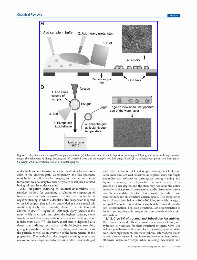
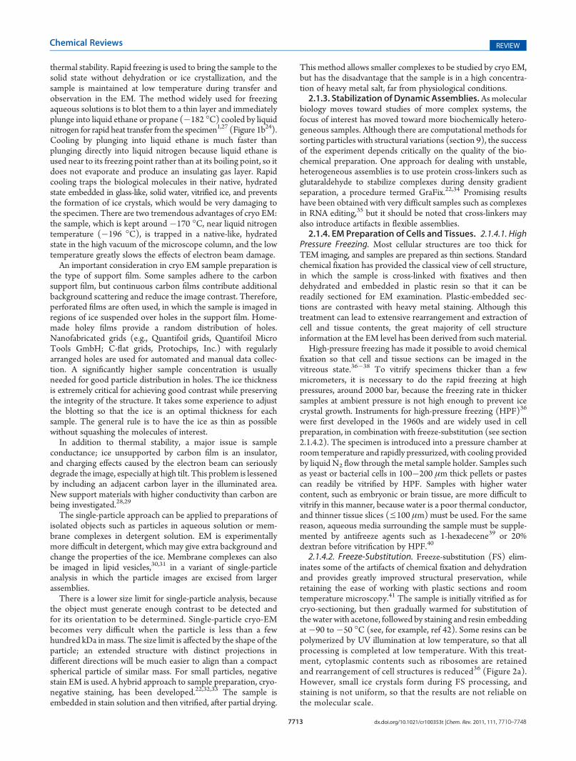
2.1.1. Negative Staining of Isolated Assemblies. Thesimplest method for examining a solution or suspension ofisolated particles such as viruses or other macromolecules isnegative staining, in which a droplet of the suspension is spreadon an EM support film and then embedded in a heavy metal saltsolution, typically uranyl acetate, blotted to a thin film andallowed to dry23,24 (Figure 1a). Although uranyl acetate is themost widely used stain and gives the highest contrast, somestructures are better preserved in other stains such as tungsten ormolybdenum salts.25,26 The heavy metal stain is deposited as adense coat outlining the surfaces of the biological assembly,giving information about the size, shape, and symmetry ofthe particle, as well as an overview of the homogeneity of thepreparation. The method is called negative staining because themacromolecular shape is seen by exclusion rather than binding of
stain. The method is quick and simple, although not foolproof.Some molecules are well preserved in negative stain, but fragileassemblies can collapse or disintegrate during staining anddrying. In general, the 3D structure becomes flattened to agreater or lesser degree, and the stain may not cover the entiremolecule, so that parts of the structure may be distorted or absentfrom the image data. Therefore, it is normally preferable to usecryo-methods for 3D structure determination. The exception isfor small structures, below ∼100�200 kDa, for which the signalin cryo-EM may be too weak for accurate detection and orienta-tion determination. For such structures, 3D reconstruction isdone from negative stain images and can provide much usefulinformation.2.1.2. Cryo EM of Isolated and Subcellular Assemblies.
Macromolecules and cells are normally in aqueous solution, andhydration is necessary for their structural integrity. Cryo EMmakes it possible to stabilize samples in the native, hydrated state,even under high vacuum. The main technical effort of cryo EM isto keep the specimen cold and free of surface contamination in anotherwise warm microscope while retaining mechanical and
Figure 1. Negative stain and cryo EM sample preparation. (a) Schematic view of sample deposition, staining, and drying, with an example negative stainimage. (b) Schematic of plunge freezing and of a vitrified layer, and an example cryo EM image. Panel (b) is adapted with permission from ref 24.Copyright 2000 International Union of Crystallography.
7713 dx.doi.org/10.1021/cr100353t |Chem. Rev. 2011, 111, 7710–7748
Chemical Reviews REVIEW
thermal stability. Rapid freezing is used to bring the sample to thesolid state without dehydration or ice crystallization, and thesample is maintained at low temperature during transfer andobservation in the EM. The method widely used for freezingaqueous solutions is to blot them to a thin layer and immediatelyplunge into liquid ethane or propane (�182 �C) cooled by liquidnitrogen for rapid heat transfer from the specimen1,27 (Figure 1b24).Cooling by plunging into liquid ethane is much faster thanplunging directly into liquid nitrogen because liquid ethane isused near to its freezing point rather than at its boiling point, so itdoes not evaporate and produce an insulating gas layer. Rapidcooling traps the biological molecules in their native, hydratedstate embedded in glass-like, solid water, vitrified ice, and preventsthe formation of ice crystals, which would be very damaging tothe specimen. There are two tremendous advantages of cryo EM:the sample, which is kept around �170 �C, near liquid nitrogentemperature (�196 �C), is trapped in a native-like, hydratedstate in the high vacuum of the microscope column, and the lowtemperature greatly slows the effects of electron beam damage.An important consideration in cryo EM sample preparation is
the type of support film. Some samples adhere to the carbonsupport film, but continuous carbon films contribute additionalbackground scattering and reduce the image contrast. Therefore,perforated films are often used, in which the sample is imaged inregions of ice suspended over holes in the support film. Home-made holey films provide a random distribution of holes.Nanofabricated grids (e.g., Quantifoil grids, Quantifoil MicroTools GmbH; C-flat grids, Protochips, Inc.) with regularlyarranged holes are used for automated and manual data collec-tion. A significantly higher sample concentration is usuallyneeded for good particle distribution in holes. The ice thicknessis extremely critical for achieving good contrast while preservingthe integrity of the structure. It takes some experience to adjustthe blotting so that the ice is an optimal thickness for eachsample. The general rule is to have the ice as thin as possiblewithout squashing the molecules of interest.In addition to thermal stability, a major issue is sample
conductance; ice unsupported by carbon film is an insulator,and charging effects caused by the electron beam can seriouslydegrade the image, especially at high tilt. This problem is lessenedby including an adjacent carbon layer in the illuminated area.New support materials with higher conductivity than carbon arebeing investigated.28,29
The single-particle approach can be applied to preparations ofisolated objects such as particles in aqueous solution or mem-brane complexes in detergent solution. EM is experimentallymore difficult in detergent, which may give extra background andchange the properties of the ice. Membrane complexes can alsobe imaged in lipid vesicles,30,31 in a variant of single-particleanalysis in which the particle images are excised from largerassemblies.There is a lower size limit for single-particle analysis, because
the object must generate enough contrast to be detected andfor its orientation to be determined. Single-particle cryo-EMbecomes very difficult when the particle is less than a fewhundred kDa inmass. The size limit is affected by the shape of theparticle; an extended structure with distinct projections indifferent directions will be much easier to align than a compactspherical particle of similar mass. For small particles, negativestain EM is used. A hybrid approach to sample preparation, cryo-negative staining, has been developed.22,32,33 The sample isembedded in stain solution and then vitrified, after partial drying.
This method allows smaller complexes to be studied by cryo EM,but has the disadvantage that the sample is in a high concentra-tion of heavy metal salt, far from physiological conditions.2.1.3. Stabilization of Dynamic Assemblies.Asmolecular
biology moves toward studies of more complex systems, thefocus of interest has moved toward more biochemically hetero-geneous samples. Although there are computational methods forsorting particles with structural variations (section 9), the successof the experiment depends critically on the quality of the bio-chemical preparation. One approach for dealing with unstable,heterogeneous assemblies is to use protein cross-linkers such asglutaraldehyde to stabilize complexes during density gradientseparation, a procedure termed GraFix.22,34 Promising resultshave been obtained with very difficult samples such as complexesin RNA editing,35 but it should be noted that cross-linkers mayalso introduce artifacts in flexible assemblies.2.1.4. EM Preparation of Cells and Tissues. 2.1.4.1. High
Pressure Freezing. Most cellular structures are too thick forTEM imaging, and samples are prepared as thin sections. Standardchemical fixation has provided the classical view of cell structure,in which the sample is cross-linked with fixatives and thendehydrated and embedded in plastic resin so that it can bereadily sectioned for EM examination. Plastic-embedded sec-tions are contrasted with heavy metal staining. Although thistreatment can lead to extensive rearrangement and extraction ofcell and tissue contents, the great majority of cell structureinformation at the EM level has been derived from such material.High-pressure freezing has made it possible to avoid chemical
fixation so that cell and tissue sections can be imaged in thevitreous state.36�38 To vitrify specimens thicker than a fewmicrometers, it is necessary to do the rapid freezing at highpressures, around 2000 bar, because the freezing rate in thickersamples at ambient pressure is not high enough to prevent icecrystal growth. Instruments for high-pressure freezing (HPF)36
were first developed in the 1960s and are widely used in cellpreparation, in combination with freeze-substitution (see section2.1.4.2). The specimen is introduced into a pressure chamber atroom temperature and rapidly pressurized, with cooling providedby liquid N2 flow through the metal sample holder. Samples suchas yeast or bacterial cells in 100�200 μm thick pellets or pastescan readily be vitrified by HPF. Samples with higher watercontent, such as embryonic or brain tissue, are more difficult tovitrify in this manner, because water is a poor thermal conductor,and thinner tissue slices (e100 μm) must be used. For the samereason, aqueous media surrounding the sample must be supple-mented by antifreeze agents such as 1-hexadecene39 or 20%dextran before vitrification by HPF.40
2.1.4.2. Freeze-Substitution. Freeze-substitution (FS) elim-inates some of the artifacts of chemical fixation and dehydrationand provides greatly improved structural preservation, whileretaining the ease of working with plastic sections and roomtemperature microscopy.41 The sample is initially vitrified as forcryo-sectioning, but then gradually warmed for substitution ofthe water with acetone, followed by staining and resin embeddingat�90 to�50 �C (see, for example, ref 42). Some resins can bepolymerized by UV illumination at low temperature, so that allprocessing is completed at low temperature. With this treat-ment, cytoplasmic contents such as ribosomes are retainedand rearrangement of cell structures is reduced36 (Figure 2a).However, small ice crystals form during FS processing, andstaining is not uniform, so that the results are not reliable onthe molecular scale.
7714 dx.doi.org/10.1021/cr100353t |Chem. Rev. 2011, 111, 7710–7748
Chemical Reviews REVIEW
Importantly, antigenicity is often conserved in FS material, sothat immunolabeling or other chemical labeling can be done onthe sections.36 This is a major advantage over vitreous sectioning,for which antibody labeling is impossible. FS is an importantadjunct to cryo-sectioning for tomography of cell structures,because large volumes are far more readily imaged and structuresof interest tracked in the 200�300 nm thick sections that can beexamined with FS. In addition, the fluorescence of GFP isretained in the freeze-substituted sections, facilitating correlativefluorescence/EM.43 A chemical reaction of the GFP chromo-phore with diaminobenzidine produces an electron dense pro-duct, allowing GFP tags to be precisely localized in EM sections.44
Therefore, the combination of cryo-sectioning and freeze-sub-stitution on the same sample can provide an overview of the 3Dstructure, chemical labeling, and detailed structural informationon regions of interest.2.1.4.3. Cryo-Sectioning of Frozen-Hydrated Specimens.
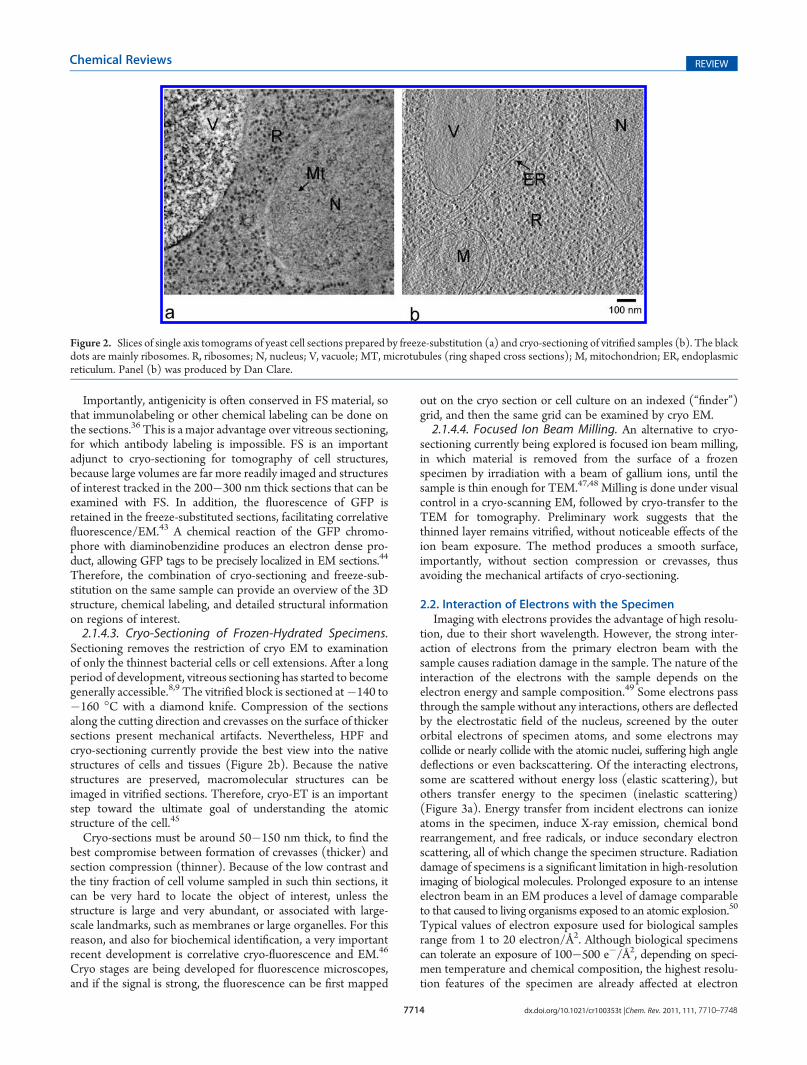
Sectioning removes the restriction of cryo EM to examinationof only the thinnest bacterial cells or cell extensions. After a longperiod of development, vitreous sectioning has started to becomegenerally accessible.8,9 The vitrified block is sectioned at�140 to�160 �C with a diamond knife. Compression of the sectionsalong the cutting direction and crevasses on the surface of thickersections present mechanical artifacts. Nevertheless, HPF andcryo-sectioning currently provide the best view into the nativestructures of cells and tissues (Figure 2b). Because the nativestructures are preserved, macromolecular structures can beimaged in vitrified sections. Therefore, cryo-ET is an importantstep toward the ultimate goal of understanding the atomicstructure of the cell.45
Cryo-sections must be around 50�150 nm thick, to find thebest compromise between formation of crevasses (thicker) andsection compression (thinner). Because of the low contrast andthe tiny fraction of cell volume sampled in such thin sections, itcan be very hard to locate the object of interest, unless thestructure is large and very abundant, or associated with large-scale landmarks, such as membranes or large organelles. For thisreason, and also for biochemical identification, a very importantrecent development is correlative cryo-fluorescence and EM.46
Cryo stages are being developed for fluorescence microscopes,and if the signal is strong, the fluorescence can be first mapped
out on the cryo section or cell culture on an indexed (“finder”)grid, and then the same grid can be examined by cryo EM.2.1.4.4. Focused Ion Beam Milling. An alternative to cryo-
sectioning currently being explored is focused ion beam milling,in which material is removed from the surface of a frozenspecimen by irradiation with a beam of gallium ions, until thesample is thin enough for TEM.47,48 Milling is done under visualcontrol in a cryo-scanning EM, followed by cryo-transfer to theTEM for tomography. Preliminary work suggests that thethinned layer remains vitrified, without noticeable effects of theion beam exposure. The method produces a smooth surface,importantly, without section compression or crevasses, thusavoiding the mechanical artifacts of cryo-sectioning.
2.2. Interaction of Electrons with the SpecimenImaging with electrons provides the advantage of high resolu-
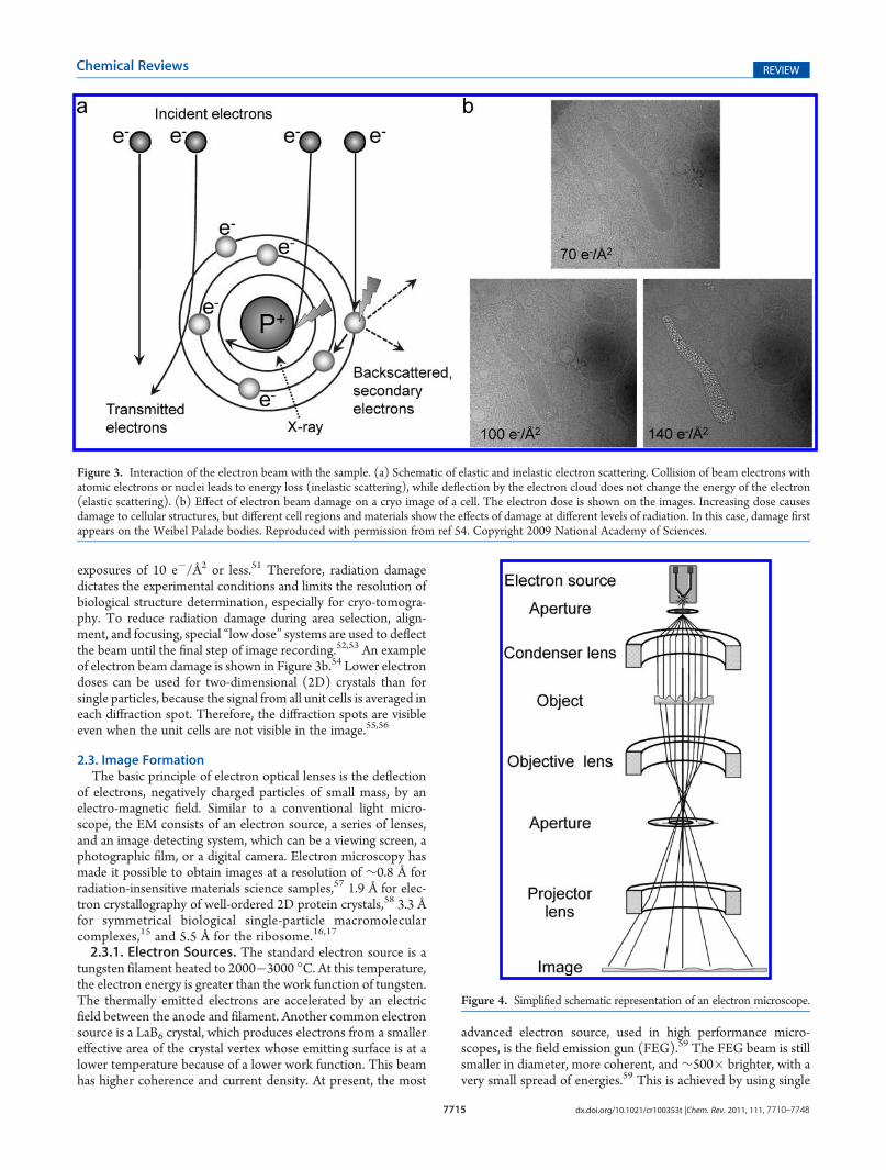
tion, due to their short wavelength. However, the strong inter-action of electrons from the primary electron beam with thesample causes radiation damage in the sample. The nature of theinteraction of the electrons with the sample depends on theelectron energy and sample composition.49 Some electrons passthrough the sample without any interactions, others are deflectedby the electrostatic field of the nucleus, screened by the outerorbital electrons of specimen atoms, and some electrons maycollide or nearly collide with the atomic nuclei, suffering high angledeflections or even backscattering. Of the interacting electrons,some are scattered without energy loss (elastic scattering), butothers transfer energy to the specimen (inelastic scattering)(Figure 3a). Energy transfer from incident electrons can ionizeatoms in the specimen, induce X-ray emission, chemical bondrearrangement, and free radicals, or induce secondary electronscattering, all of which change the specimen structure. Radiationdamage of specimens is a significant limitation in high-resolutionimaging of biological molecules. Prolonged exposure to an intenseelectron beam in an EM produces a level of damage comparableto that caused to living organisms exposed to an atomic explosion.50
Typical values of electron exposure used for biological samplesrange from 1 to 20 electron/Å2. Although biological specimenscan tolerate an exposure of 100�500 e�/Å2, depending on speci-men temperature and chemical composition, the highest resolu-tion features of the specimen are already affected at electron
Figure 2. Slices of single axis tomograms of yeast cell sections prepared by freeze-substitution (a) and cryo-sectioning of vitrified samples (b). The blackdots are mainly ribosomes. R, ribosomes; N, nucleus; V, vacuole; MT, microtubules (ring shaped cross sections); M, mitochondrion; ER, endoplasmicreticulum. Panel (b) was produced by Dan Clare.
7715 dx.doi.org/10.1021/cr100353t |Chem. Rev. 2011, 111, 7710–7748
Chemical Reviews REVIEW
exposures of 10 e�/Å2 or less.51 Therefore, radiation damagedictates the experimental conditions and limits the resolution ofbiological structure determination, especially for cryo-tomogra-phy. To reduce radiation damage during area selection, align-ment, and focusing, special “low dose” systems are used to deflectthe beam until the final step of image recording.52,53 An exampleof electron beam damage is shown in Figure 3b.54 Lower electrondoses can be used for two-dimensional (2D) crystals than forsingle particles, because the signal from all unit cells is averaged ineach diffraction spot. Therefore, the diffraction spots are visibleeven when the unit cells are not visible in the image.55,56
2.3. Image FormationThe basic principle of electron optical lenses is the deflection
of electrons, negatively charged particles of small mass, by anelectro-magnetic field. Similar to a conventional light micro-scope, the EM consists of an electron source, a series of lenses,and an image detecting system, which can be a viewing screen, aphotographic film, or a digital camera. Electron microscopy hasmade it possible to obtain images at a resolution of ∼0.8 Å forradiation-insensitive materials science samples,57 1.9 Å for elec-tron crystallography of well-ordered 2D protein crystals,58 3.3 Åfor symmetrical biological single-particle macromolecularcomplexes,15 and 5.5 Å for the ribosome.16,17
2.3.1. Electron Sources. The standard electron source is atungsten filament heated to 2000�3000 �C. At this temperature,the electron energy is greater than the work function of tungsten.The thermally emitted electrons are accelerated by an electricfield between the anode and filament. Another common electronsource is a LaB6 crystal, which produces electrons from a smallereffective area of the crystal vertex whose emitting surface is at alower temperature because of a lower work function. This beamhas higher coherence and current density. At present, the most
advanced electron source, used in high performance micro-scopes, is the field emission gun (FEG).59 The FEG beam is stillsmaller in diameter, more coherent, and∼500� brighter, with avery small spread of energies.59 This is achieved by using single
Figure 4. Simplified schematic representation of an electron microscope.
Figure 3. Interaction of the electron beam with the sample. (a) Schematic of elastic and inelastic electron scattering. Collision of beam electrons withatomic electrons or nuclei leads to energy loss (inelastic scattering), while deflection by the electron cloud does not change the energy of the electron(elastic scattering). (b) Effect of electron beam damage on a cryo image of a cell. The electron dose is shown on the images. Increasing dose causesdamage to cellular structures, but different cell regions and materials show the effects of damage at different levels of radiation. In this case, damage firstappears on the Weibel Palade bodies. Reproduced with permission from ref 54. Copyright 2009 National Academy of Sciences.
7716 dx.doi.org/10.1021/cr100353t |Chem. Rev. 2011, 111, 7710–7748
Chemical Reviews REVIEW
crystal tungsten sharpened to give a tip radius ∼10�25 nm, ascompared to 5�10 μm for LaB6 crystals. The tip is coated withZrO2, which lowers the work function for electrons. Thermallyemitted electrons are extracted from the crystal tip by a strongpotential gradient at the emitter surface (field emission), andthen accelerated through voltages of 100�300 kV.2.3.2. The Electron Microscope Lens System. As in light
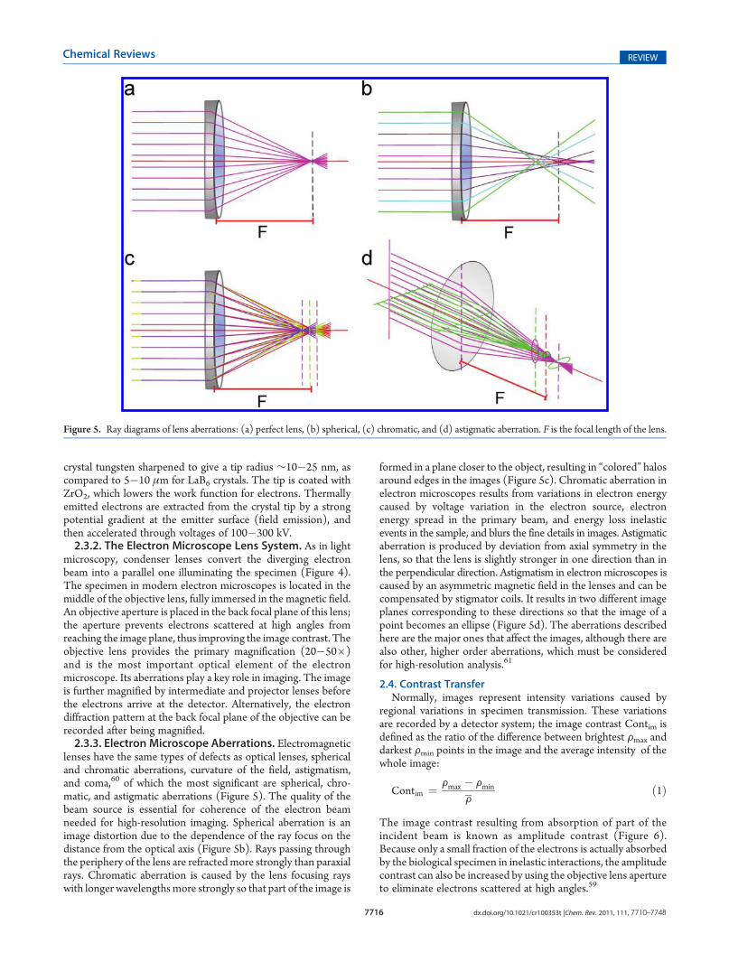
microscopy, condenser lenses convert the diverging electronbeam into a parallel one illuminating the specimen (Figure 4).The specimen in modern electron microscopes is located in themiddle of the objective lens, fully immersed in the magnetic field.An objective aperture is placed in the back focal plane of this lens;the aperture prevents electrons scattered at high angles fromreaching the image plane, thus improving the image contrast. Theobjective lens provides the primary magnification (20�50�)and is the most important optical element of the electronmicroscope. Its aberrations play a key role in imaging. The imageis further magnified by intermediate and projector lenses beforethe electrons arrive at the detector. Alternatively, the electrondiffraction pattern at the back focal plane of the objective can berecorded after being magnified.2.3.3. Electron Microscope Aberrations. Electromagnetic
lenses have the same types of defects as optical lenses, sphericaland chromatic aberrations, curvature of the field, astigmatism,and coma,60 of which the most significant are spherical, chro-matic, and astigmatic aberrations (Figure 5). The quality of thebeam source is essential for coherence of the electron beamneeded for high-resolution imaging. Spherical aberration is animage distortion due to the dependence of the ray focus on thedistance from the optical axis (Figure 5b). Rays passing throughthe periphery of the lens are refractedmore strongly than paraxialrays. Chromatic aberration is caused by the lens focusing rayswith longer wavelengthsmore strongly so that part of the image is
formed in a plane closer to the object, resulting in “colored” halosaround edges in the images (Figure 5c). Chromatic aberration inelectron microscopes results from variations in electron energycaused by voltage variation in the electron source, electronenergy spread in the primary beam, and energy loss inelasticevents in the sample, and blurs the fine details in images. Astigmaticaberration is produced by deviation from axial symmetry in thelens, so that the lens is slightly stronger in one direction than inthe perpendicular direction. Astigmatism in electron microscopes iscaused by an asymmetric magnetic field in the lenses and can becompensated by stigmator coils. It results in two different imageplanes corresponding to these directions so that the image of apoint becomes an ellipse (Figure 5d). The aberrations describedhere are the major ones that affect the images, although there arealso other, higher order aberrations, which must be consideredfor high-resolution analysis.61
2.4. Contrast TransferNormally, images represent intensity variations caused by
regional variations in specimen transmission. These variationsare recorded by a detector system; the image contrast Contim isdefined as the ratio of the difference between brightest Fmax anddarkest Fmin points in the image and the average intensity of thewhole image:
Contim ¼ Fmax � FminF
ð1Þ
The image contrast resulting from absorption of part of theincident beam is known as amplitude contrast (Figure 6).Because only a small fraction of the electrons is actually absorbedby the biological specimen in inelastic interactions, the amplitudecontrast can also be increased by using the objective lens apertureto eliminate electrons scattered at high angles.59
Figure 5. Ray diagrams of lens aberrations: (a) perfect lens, (b) spherical, (c) chromatic, and (d) astigmatic aberration. F is the focal length of the lens.
7717 dx.doi.org/10.1021/cr100353t |Chem. Rev. 2011, 111, 7710–7748
Chemical Reviews REVIEW
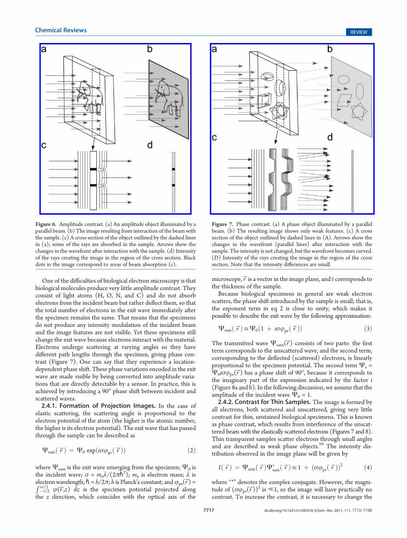
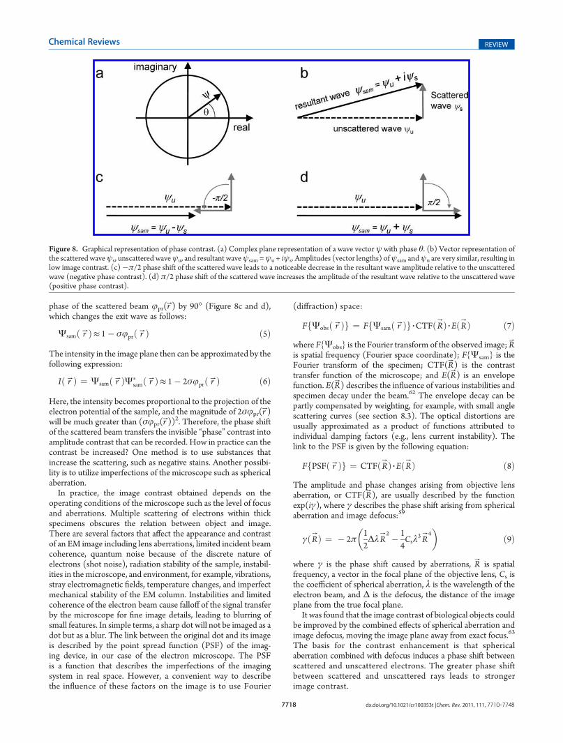
One of the difficulties of biological electron microscopy is thatbiological molecules produce very little amplitude contrast. Theyconsist of light atoms (H, O, N, and C) and do not absorbelectrons from the incident beam but rather deflect them, so thatthe total number of electrons in the exit wave immediately afterthe specimen remains the same. That means that the specimensdo not produce any intensity modulation of the incident beamand the image features are not visible. Yet these specimens stillchange the exit wave because electrons interact with the material.Electrons undergo scattering at varying angles so they havedifferent path lengths through the specimen, giving phase con-trast (Figure 7). One can say that they experience a location-dependent phase shift. These phase variations encoded in the exitwave are made visible by being converted into amplitude varia-tions that are directly detectable by a sensor. In practice, this isachieved by introducing a 90� phase shift between incident andscattered waves.2.4.1. Formation of Projection Images. In the case of
elastic scattering, the scattering angle is proportional to theelectron potential of the atom (the higher is the atomic number,the higher is its electron potential). The exit wave that has passedthrough the sample can be described as
Ψsamð rBÞ ¼ Ψ0 expðiσjprð rBÞÞ ð2Þ
whereΨsam is the exit wave emerging from the specimen;Ψ0 isthe incident wave; σ = meλ/(2πp
2); me is electron mass; λ iselectron wavelength; p = h/2π; h is Planck’s constant; andjpr(rB) =R�t/2+t/2 j(rB,z) dz is the specimen potential projected along
the z direction, which coincides with the optical axis of the
microscope, rB is a vector in the image plane, and t corresponds tothe thickness of the sample.Because biological specimens in general are weak electron
scatters, the phase shift introduced by the sample is small; that is,the exponent term in eq 2 is close to unity, which makes itpossible to describe the exit wave by the following approximation:
Ψsamð rBÞ≈Ψ0ð1 þ iσjprð rBÞÞ ð3Þ
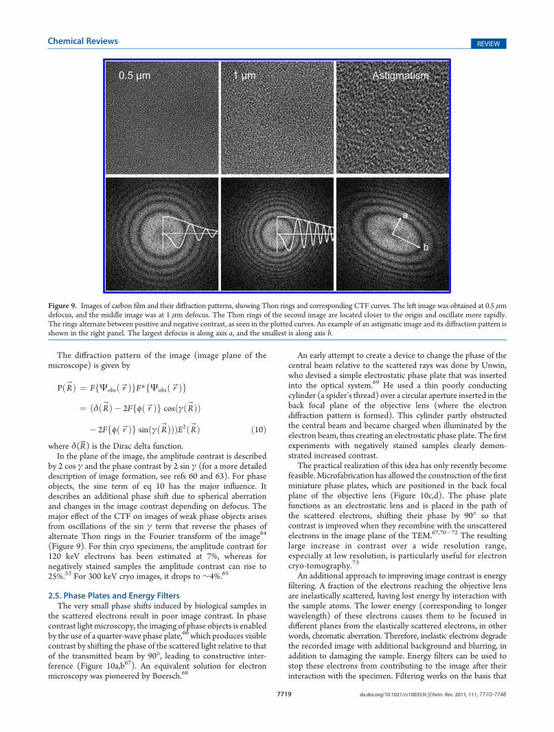
The transmitted wave Ψsam(rB) consists of two parts: the firstterm corresponds to the unscattered wave, and the second term,corresponding to the deflected (scattered) electrons, is linearlyproportional to the specimen potential. The second term Ψs =Ψ0iσjpr(rB) has a phase shift of 90�, because it corresponds tothe imaginary part of the expression indicated by the factor i(Figure 8a and b). In the following discussion, we assume that theamplitude of the incident wave Ψ0 = 1.2.4.2. Contrast for Thin Samples. The image is formed by
all electrons, both scattered and unscattered, giving very littlecontrast for thin, unstained biological specimens. This is knownas phase contrast, which results from interference of the unscat-tered beamwith the elastically scattered electrons (Figures 7 and 8).Thin transparent samples scatter electrons through small anglesand are described as weak phase objects.59 The intensity dis-tribution observed in the image plane will be given by
Ið rBÞ ¼ Ψsamð rBÞΨ�samð rBÞ≈ 1 þ ðσjprð rBÞÞ2 ð4Þ
where “*” denotes the complex conjugate. However, the magni-tude of (σjpr(rB))
2 is ,1, so the image will have practically nocontrast. To increase the contrast, it is necessary to change the
Figure 7. Phase contrast. (a) A phase object illuminated by a parallelbeam. (b) The resulting image shows only weak features. (c) A crosssection of the object outlined by dashed lines in (A). Arrows show thechanges in the wavefront (parallel lines) after interaction with thesample. The intensity is not changed, but the wavefront becomes curved.(D) Intensity of the rays creating the image in the region of the crosssection. Note that the intensity differences are small.
Figure 6. Amplitude contrast. (a) An amplitude object illuminated by aparallel beam. (b) The image resulting from interaction of the beamwiththe sample. (c) A cross section of the object outlined by the dashed linesin (a); some of the rays are absorbed in the sample. Arrows show thechanges in the wavefront after interaction with the sample. (d) Intensityof the rays creating the image in the region of the cross section. Blackdots in the image correspond to areas of beam absorption (c).
7718 dx.doi.org/10.1021/cr100353t |Chem. Rev. 2011, 111, 7710–7748
Chemical Reviews REVIEW
phase of the scattered beam jpr(rB) by 90� (Figure 8c and d),which changes the exit wave as follows:
Ψsamð rBÞ≈ 1� σjprð rBÞ ð5ÞThe intensity in the image plane then can be approximated by thefollowing expression:
Ið rBÞ ¼ Ψsamð rBÞΨ�samð rBÞ≈ 1� 2σjprð rBÞ ð6Þ
Here, the intensity becomes proportional to the projection of theelectron potential of the sample, and the magnitude of 2σjpr(rB)will be much greater than (σjpr(rB))
2. Therefore, the phase shiftof the scattered beam transfers the invisible “phase” contrast intoamplitude contrast that can be recorded. How in practice can thecontrast be increased? One method is to use substances thatincrease the scattering, such as negative stains. Another possibi-lity is to utilize imperfections of the microscope such as sphericalaberration.In practice, the image contrast obtained depends on the
operating conditions of the microscope such as the level of focusand aberrations. Multiple scattering of electrons within thickspecimens obscures the relation between object and image.There are several factors that affect the appearance and contrastof an EM image including lens aberrations, limited incident beamcoherence, quantum noise because of the discrete nature ofelectrons (shot noise), radiation stability of the sample, instabil-ities in themicroscope, and environment, for example, vibrations,stray electromagnetic fields, temperature changes, and imperfectmechanical stability of the EM column. Instabilities and limitedcoherence of the electron beam cause falloff of the signal transferby the microscope for fine image details, leading to blurring ofsmall features. In simple terms, a sharp dot will not be imaged as adot but as a blur. The link between the original dot and its imageis described by the point spread function (PSF) of the imag-ing device, in our case of the electron microscope. The PSFis a function that describes the imperfections of the imagingsystem in real space. However, a convenient way to describethe influence of these factors on the image is to use Fourier
(diffraction) space:
FfΨobsð rBÞg ¼ FfΨsamð rBÞg 3CTFðRBÞ 3 EðRBÞ ð7Þwhere F{Ψobs} is the Fourier transform of the observed image; RBis spatial frequency (Fourier space coordinate); F{Ψsam} is theFourier transform of the specimen; CTF(RB) is the contrasttransfer function of the microscope; and E(RB) is an envelopefunction. E(RB) describes the influence of various instabilities andspecimen decay under the beam.62 The envelope decay can bepartly compensated by weighting, for example, with small anglescattering curves (see section 8.3). The optical distortions areusually approximated as a product of functions attributed toindividual damping factors (e.g., lens current instability). Thelink to the PSF is given by the following equation:
FfPSFð rBÞg ¼ CTFðRBÞ 3 EðRBÞ ð8ÞThe amplitude and phase changes arising from objective lensaberration, or CTF(RB), are usually described by the functionexp(iγ), where γ describes the phase shift arising from sphericalaberration and image defocus:59
γðRBÞ ¼ � 2π12ΔλRB
2 � 14Csλ
3RB4
� �ð9Þ
where γ is the phase shift caused by aberrations, RB is spatialfrequency, a vector in the focal plane of the objective lens, Cs isthe coefficient of spherical aberration, λ is the wavelength of theelectron beam, and Δ is the defocus, the distance of the imageplane from the true focal plane.It was found that the image contrast of biological objects could
be improved by the combined effects of spherical aberration andimage defocus, moving the image plane away from exact focus.63
The basis for the contrast enhancement is that sphericalaberration combined with defocus induces a phase shift betweenscattered and unscattered electrons. The greater phase shiftbetween scattered and unscattered rays leads to strongerimage contrast.
Figure 8. Graphical representation of phase contrast. (a) Complex plane representation of a wave vectorψ with phase θ. (b) Vector representation ofthe scattered waveψs, unscattered waveψu, and resultant waveψsam =ψu + iψs. Amplitudes (vector lengths) ofψsam andψu are very similar, resulting inlow image contrast. (c)�π/2 phase shift of the scattered wave leads to a noticeable decrease in the resultant wave amplitude relative to the unscatteredwave (negative phase contrast). (d) π/2 phase shift of the scattered wave increases the amplitude of the resultant wave relative to the unscattered wave(positive phase contrast).
7719 dx.doi.org/10.1021/cr100353t |Chem. Rev. 2011, 111, 7710–7748
Chemical Reviews REVIEW
The diffraction pattern of the image (image plane of themicroscope) is given by
PðRBÞ ¼ FfΨobsð rBÞgF�fΨobsð rBÞg
¼ ðδðRBÞ � 2Ffϕð rBÞg cosðγðRBÞÞ
� 2Ffϕð rBÞg sinðγðRBÞÞÞE2ðRBÞ ð10Þwhere δ(RB) is the Dirac delta function.In the plane of the image, the amplitude contrast is described
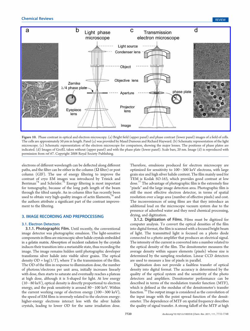
by 2 cos γ and the phase contrast by 2 sin γ (for a more detaileddescription of image formation, see refs 60 and 63). For phaseobjects, the sine term of eq 10 has the major influence. Itdescribes an additional phase shift due to spherical aberrationand changes in the image contrast depending on defocus. Themajor effect of the CTF on images of weak phase objects arisesfrom oscillations of the sin γ term that reverse the phases ofalternate Thon rings in the Fourier transform of the image64
(Figure 9). For thin cryo specimens, the amplitude contrast for120 keV electrons has been estimated at 7%, whereas fornegatively stained samples the amplitude contrast can rise to25%.53 For 300 keV cryo images, it drops to ∼4%.65
2.5. Phase Plates and Energy FiltersThe very small phase shifts induced by biological samples in
the scattered electrons result in poor image contrast. In phasecontrast light microscopy, the imaging of phase objects is enabledby the use of a quarter-wave phase plate,66 which produces visiblecontrast by shifting the phase of the scattered light relative to thatof the transmitted beam by 90�, leading to constructive inter-ference (Figure 10a,b67). An equivalent solution for electronmicroscopy was pioneered by Boersch.68
An early attempt to create a device to change the phase of thecentral beam relative to the scattered rays was done by Unwin,who devised a simple electrostatic phase plate that was insertedinto the optical system.69 He used a thin poorly conductingcylinder (a spider’s thread) over a circular aperture inserted in theback focal plane of the objective lens (where the electrondiffraction pattern is formed). This cylinder partly obstructedthe central beam and became charged when illuminated by theelectron beam, thus creating an electrostatic phase plate. The firstexperiments with negatively stained samples clearly demon-strated increased contrast.
The practical realization of this idea has only recently becomefeasible. Microfabrication has allowed the construction of the firstminiature phase plates, which are positioned in the back focalplane of the objective lens (Figure 10c,d). The phase platefunctions as an electrostatic lens and is placed in the path ofthe scattered electrons, shifting their phase by 90� so thatcontrast is improved when they recombine with the unscatteredelectrons in the image plane of the TEM.67,70�72 The resultinglarge increase in contrast over a wide resolution range,especially at low resolution, is particularly useful for electroncryo-tomography.73
An additional approach to improving image contrast is energyfiltering. A fraction of the electrons reaching the objective lensare inelastically scattered, having lost energy by interaction withthe sample atoms. The lower energy (corresponding to longerwavelength) of these electrons causes them to be focused indifferent planes from the elastically scattered electrons, in otherwords, chromatic aberration. Therefore, inelastic electrons degradethe recorded image with additional background and blurring, inaddition to damaging the sample. Energy filters can be used tostop these electrons from contributing to the image after theirinteraction with the specimen. Filtering works on the basis that
Figure 9. Images of carbon film and their diffraction patterns, showing Thon rings and corresponding CTF curves. The left image was obtained at 0.5 μmdefocus, and the middle image was at 1 μm defocus. The Thon rings of the second image are located closer to the origin and oscillate more rapidly.The rings alternate between positive and negative contrast, as seen in the plotted curves. An example of an astigmatic image and its diffraction pattern isshown in the right panel. The largest defocus is along axis a, and the smallest is along axis b.
7720 dx.doi.org/10.1021/cr100353t |Chem. Rev. 2011, 111, 7710–7748
Chemical Reviews REVIEW
electrons of different wavelength can be deflected along differentpaths, and the filter can be either in the column (Ω filter) or postcolumn (GIF). The use of energy filtering to improve thecontrast of cryo EM images was introduced by Trinick andBerriman74 and Schr€oder.75 Energy filtering is most importantfor tomography, because of the long path length of the beamthrough the tilted sample. An in-column filter has recently beenused to obtain very high-quality images of actin filaments,76 andthe authors attribute a significant part of the contrast improve-ment to the filtering.
3. IMAGE RECORDING AND PREPROCESSING
3.1. Electron Detectors3.1.1. Photographic Film. Until recently, the conventional
image detector was photographic emulsion. The light-sensitivecomponents in films aremicroscopic silver halide crystals embeddedin a gelatin matrix. Absorption of incident radiation by the crystalsinduces their transition into ametastable state, thus recording theimage. The image remains hidden until photographic developertransforms silver halide into visible silver grains. The opticaldensity OD = log(1/T), where T is the transmission of the film.The OD of the film in response to illumination dose, the numberof photons/electrons per unit area, initially increases linearlywith dose, then starts to saturate and eventually reaches a plateauat high dose, although it is S-shaped for light. At low energy(10�80 keV), optical density is directly proportional to electronenergy, and the peak sensitivity is around 80�100 keV. Withinthe current working range of electron energy (100�300 keV),the speed of EM films is inversely related to the electron energy:higher-energy electrons interact less with the silver halidecrystals, leading to lower OD for the same irradiation dose.
Therefore, emulsions produced for electron microscopy areoptimized for sensitivity to 100�300 keV electrons, with largegrain size and high silver halide content. The filmmainly used forTEM is Kodak SO-163, which provides good contrast at lowdose.77 The advantage of photographic film is the extremely fine“pixels” and the large image detection area. Photographic film isstill the most effective electron detector, in terms of spatialresolution over a large area (number of effective pixels) and cost.The inconveniences of using films are that they introduce anadditional load on the microscope vacuum system due to thepresence of adsorbed water and they need chemical processing,drying, and digitization.3.1.2. Digitization of Films. Films must be digitized for
computer analysis. To convert the optical densities of the filminto digital format, the film is scanned with a focused bright beamof light. The transmitted light is focused on a photo diodeconnected to a photo amplifier that produces an electrical signal.The intensity of the current is converted into a number related tothe optical density of the film. The densitometer measures theaverage density within square elements (pixels) whose size isdetermined by the sampling resolution. Linear CCD detectorsare used to measure a line of pixels in parallel.Digitisation does not provide a faultless transfer of optical
density into digital format. The accuracy is determined by thequality of the optical system and the sensitivity of the photodetectors and amplifiers. Densitometer performance can bedescribed in terms of the modulation transfer function (MTF),which is defined as the modulus of the densitometer’s transferfunction.78 The output image is considered as the convolution ofthe input image with the point spread function of the densit-ometer. The dependence of MTF on spatial frequency describesthe quality of signal transfer. A strong falloff of the MTF at high
Figure 10. Phase contrast in optical and electron microscopy. (a) Bright field (upper panel) and phase contrast (lower panel) images of a field of cells.The cells are approximately 50 μm in length. Panel (a) was provided byMaud Dumoux and Richard Hayward. (b) Schematic representation of the lightmicroscope. (c) Schematic representation of the electron microscope for comparison, showing the major lenses. The positions of phase plates areindicated. (d) Images of GroEL taken without (upper panel) and with the phase plate (lower panel). Scale bars, 20 nm. Image (d) is reproduced withpermission from ref 67. Copyright 2008 Royal Society Publishing.
7721 dx.doi.org/10.1021/cr100353t |Chem. Rev. 2011, 111, 7710–7748
Chemical Reviews REVIEW
frequencies indicates the loss of fine details in the digitizedimages. Densitometer characteristics and assessments have beendescribed in several articles.79,80
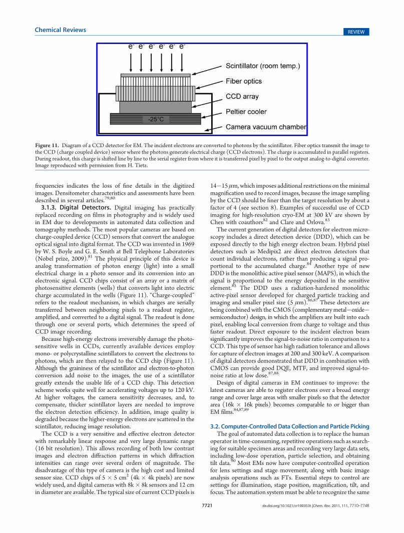
3.1.3. Digital Detectors. Digital imaging has practicallyreplaced recording on films in photography and is widely usedin EM due to developments in automated data collection andtomography methods. The most popular cameras are based oncharge-coupled device (CCD) sensors that convert the analogueoptical signal into digital format. The CCD was invented in 1969by W. S. Boyle and G. E. Smith at Bell Telephone Laboratories(Nobel prize, 2009).81 The physical principle of this device isanalog transformation of photon energy (light) into a smallelectrical charge in a photo sensor and its conversion into anelectronic signal. CCD chips consist of an array or a matrix ofphotosensitive elements (wells) that converts light into electriccharge accumulated in the wells (Figure 11). “Charge-coupled”refers to the readout mechanism, in which charges are seriallytransferred between neighboring pixels to a readout register,amplified, and converted to a digital signal. The readout is donethrough one or several ports, which determines the speed ofCCD image recording.Because high-energy electrons irreversibly damage the photo-
sensitive wells in CCDs, currently available devices employmono- or polycrystalline scintillators to convert the electrons tophotons, which are then relayed to the CCD chip (Figure 11).Although the graininess of the scintillator and electron-to-photonconversion add noise to the images, the use of a scintillatorgreatly extends the usable life of a CCD chip. This detectionscheme works quite well for accelerating voltages up to 120 kV.At higher voltages, the camera sensitivity decreases, and, tocompensate, thicker scintillator layers are needed to improvethe electron detection efficiency. In addition, image quality isdegraded because the higher-energy electrons are scattered in thescintillator, reducing image resolution.The CCD is a very sensitive and effective electron detector
with remarkably linear response and very large dynamic range(16 bit resolution). This allows recording of both low contrastimages and electron diffraction patterns in which diffractionintensities can range over several orders of magnitude. Thedisadvantage of this type of camera is the high cost and limitedsensor size. CCD chips of 5 � 5 cm2 (4k � 4k pixels) are nowwidely used, and digital cameras with 8k� 8k sensors and 12 cmin diameter are available. The typical size of current CCDpixels is
14�15 μm,which imposes additional restrictions on theminimalmagnification used to record images, because the image samplingby the CCD should be finer than the target resolution by about afactor of 4 (see section 8). Examples of successful use of CCDimaging for high-resolution cryo-EM at 300 kV are shown byChen with coauthors82 and Clare and Orlova.83
The current generation of digital detectors for electron micro-scopy includes a direct detection device (DDD), which can beexposed directly to the high energy electron beam. Hybrid pixeldetectors such as Medipix2 are direct electron detectors thatcount individual electrons, rather than producing a signal pro-portional to the accumulated charge.84 Another type of newDDD is the monolithic active pixel sensor (MAPS), in which thesignal is proportional to the energy deposited in the sensitiveelement.85 The DDD uses a radiation-hardened monolithicactive-pixel sensor developed for charged particle tracking andimaging and smaller pixel size (5 μm).86,87 These detectors arebeing combined with the CMOS (complementarymetal�oxide�semiconductor) design, in which the amplifiers are built into eachpixel, enabling local conversion from charge to voltage and thusfaster readout. Direct exposure to the incident electron beamsignificantly improves the signal-to-noise ratio in comparison to aCCD. This type of sensor has high radiation tolerance and allowsfor capture of electron images at 200 and 300 keV. A comparisonof digital detectors demonstrated that DDD in combination withCMOS can provide good DQE, MTF, and improved signal-to-noise ratio at low dose.87,88
Design of digital cameras in EM continues to improve: thelatest cameras are able to register electrons over a broad energyrange and cover large areas with smaller pixels so that the detectorarea (16k � 16k pixels) becomes comparable to or bigger thanEM films.84,87,89
3.2. Computer-Controlled Data Collection and Particle PickingThe goal of automated data collection is to replace the human
operator in time-consuming, repetitive operations such as search-ing for suitable specimen areas and recording very large data sets,including low-dose operation, particle selection, and obtainingtilt data.90 Most EMs now have computer-controlled operationfor lens settings and stage movement, along with basic imageanalysis operations such as FTs. Essential steps to control aresettings for illumination, stage position, magnification, tilt, andfocus. The automation systemmust be able to recognize the same
Figure 11. Diagram of a CCD detector for EM. The incident electrons are converted to photons by the scintillator. Fiber optics transmit the image tothe CCD (charge coupled device) sensor where the photons generate electrical charge (CCD electrons). The charge is accumulated in parallel registers.During readout, this charge is shifted line by line to the serial register from where it is transferred pixel by pixel to the output analog-to-digital converter.Image reproduced with permission from H. Tietz.
7722 dx.doi.org/10.1021/cr100353t |Chem. Rev. 2011, 111, 7710–7748
Chemical Reviews REVIEW
region at different magnification scales, so that objects selected ina lower magnification overview can be located for data collection,in particular after stage movements. The software must compen-sate for inaccuracies in mechanical stage positioning. Thiscompensation is done by collecting overview images and findingthe areas of interest by cross-correlation with previously recordedimages, so that the selected area can be positioned with sufficientprecision for high-magnification recording. For all of these opera-tions, electronic image recording is essential, and the availabilityof high-resolution CCD cameras has enabled the development ofautomation. Several automation systems have been developed,both by academic users (e.g., Leginon;90 JADAS91) and by EMsuppliers (FEI, JEOL systems). Some of them are coupled to dataprocessing pipelines that extend the automation through thestages of particle picking and image processing (e.g., Appion92).Serial EM is a widely used system that provides semiautomatedprocedures for manually selecting a series of targets for subse-quent unsupervised collection of tomograms and can also beused for single-particle data.93
In single-particle EM, data processing begins with particleselection. Conventionally, the particles are identified by shapeand characteristic features that are often difficult to recognize fora new complex. Even for known complexes, manual selection of∼100 000 single-particle images is prohibitively time-consumingand tedious. Not surprisingly, the idea of automating particleselection has been a focus of research efforts. The first computa-tional methods were based on template matching,94,95 and moresophisticated approaches were subsequently based on patternrecognition.96 A comparative evaluation of different programscan be found in the review by Zhu and coauthors,97 and otherprograms have been developed more recently.98
3.3. Tomographic Data CollectionThe purpose of electron tomography is to obtain a 3D
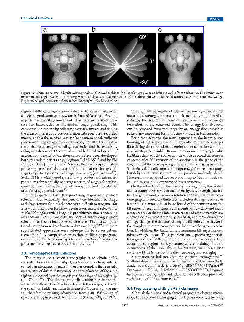
reconstruction of a unique object, such as a cell section, isolatedsubcellular structure, or macromolecular complex, that can takeup a variety of different structures. A series of images of the sameregion is recorded over the largest possible range of tilt angles, upto �70� to 70�. The limitation on tilt is ultimately due to theincreased path length of the beam through the sample, althoughthe specimen holder may also limit the tilt. Electron tomogramswill therefore be missing information from a 40�60� wedge ofspace, resulting in some distortion to the 3D map (Figure 1299).
The high tilt, especially of thicker specimens, increases theinelastic scattering and multiple elastic scattering, thereforereducing the fraction of coherent electrons useful in imageformation, in the scattered beam. The energy-loss electronscan be removed from the image by an energy filter, which isparticularly important for improving contrast in tomography.
For plastic sections, the initial exposure to the beam causesthinning of the sections, but subsequently the sample changeslittle during data collection. Therefore, data collection with fineangular steps is possible. Room temperature tomography alsofacilitates dual-axis data collection, in which a second tilt series iscollected after 90� rotation of the specimen in the plane of thestage, so that the missing wedge is reduced to a missing pyramid.Therefore, data collection can be optimized for plastic sections,but dehydration and staining do not preserve molecular detail.However, as mentioned above, sections up to 300 nm thick canbe used to give a 3D overview of larger structures.
On the other hand, in electron cryo-tomography, the molec-ular structure is preserved in the frozen-hydrated sample, but it ishard to get beyond 3�4 nm resolution. The resolution of cryo-tomography is severely limited by radiation damage, because atleast 50�100 images must be collected of the same area for thetilt series. These conflicting requirements for low dose and manyexposures mean that the images are recorded with extremely lowelectron dose and therefore very low SNR, and the accumulateddamage changes the structure during the tilt series. The thicker isthe sample, the more views are needed to reach a given resolu-tion. In addition, the limitation on maximum tilt angle leaves amissing wedge of data. These problems make processing of cryo-tomograms more difficult. The best resolution is obtained byaveraging subregions of cryo-tomograms containing multipleoccurrences of the same object, for example, viral spikes (seesection 4.4). This method is called subtomogram averaging.
Automation is indispensable for electron tomography.100
Well-developed tomography software is available from bothacademic and commercial sources (SerialEM;93 UCSFTomo;101
Protomo;102 TOM;103 Xplore3D;104 IMOD105,106). Leginonincorporates tomographic and other tilt data collection protocolssuch as conical tilt (section 6.1).107
3.4. Preprocessing of Single-Particle ImagesAlthough theoretical and technical progress in electron micro-
scopy has improved the imaging of weak phase objects, defocusing
Figure 12. Distortions caused by the missing wedge. (a) A model object. (b) Set of image planes at different angles from a tilt series. The limitation onmaximum tilt angle results in a missing wedge of data. (c) Reconstruction of the object showing elongated features due to the missing wedge.Reproduced with permission from ref 99. Copyright 1998 Elsevier Inc.
7723 dx.doi.org/10.1021/cr100353t |Chem. Rev. 2011, 111, 7710–7748
Chemical Reviews REVIEW
complicates the interpretation of the image because features insome size ranges will have reversed contrast. Imaging of biolo-gical objects requires a compromise between contrast enhance-ment and minimization of image distortions.
The intensity distribution in the EM image plane is related tothe projected electron potential by
Ið rBÞ ¼ Ψobsð rBÞΨ�obsð rBÞ≈ 1 þ σjprð rBÞ X F�1fsin γg
ð11Þwhere sinγ is the phase contrast transfer function andγ is definedby eq 9. F�1{sinγ} defines the shape of the image of a point in theobject plane formed by the microscope optics, the point spreadfunction (PSF) of the microscope. Therefore, the real image isdistorted, because the ideal object image is convoluted withthe PSF, and is not directly related to the density distribution inthe original object. To restore the image, so that it corresponds tothe projected electron potential of the sample, the image must becorrected for the effect of contrast modulation by sin γ, themicroscope phase contrast transfer function (CTF). The CTF,modified by an envelope decay, and the PSF of a microscope arerelated by Fourier transformation. For weak phase objects,deconvolution with the PSF of the microscope is necessary forcomplete restoration of image data. The procedure of eliminatingthe effects of the CTF is called CTF correction.3.4.1. Determination of the CTF. For a given microscope
setup, the voltage and spherical aberration are constant, but thedefocus varies from image to image because of variations in lenssettings, sample height, and thickness. There are two mainapproaches for determination and correction of the CTF. Inthe first one, the images are CTF-corrected before structuralanalysis. In the second approach, structural analysis is doneseparately on each micrograph, and determination and correc-tion of the CTF are performed on the structures obtained. Eachapproach has its own advantages and disadvantages.If CTF correction is done first, data can be combined from
many different micrographs and subsequently processed to-gether. The second method is applicable if each micrographhas a sufficient number of particles to calculate a 3D reconstruc-tion. This method works well for particles at high concentrationand has the advantage that CTF determination is more accuratebecause of the high SNR in the reconstruction, in which theimages have been combined. However, with fewer particles andlower symmetry, it will not be possible to get a good reconstruc-tion of the object from a single micrograph, so that the firstapproach is more practical.Manual CTF determination108 involves calculation of the
rotationally averaged power spectrum (diffraction intensity) ofa set of 2D images, which can only be done in the absence ofastigmatism. The amplitude profile (square root of the inten-sities) is compared to a model CTF. The model defocus is variedto find the best match between the two profiles. The valuecorresponding to the match is then used as the defocus for thatparticular set of images. It is also possible to include additionalprocessing steps such as band-pass filtering to remove back-ground and provide smoothing for more accurate detection ofthe positions of the CTF minima.The rotational averaging used in the above method assumes
good astigmatism correction. Software developed byMindell andGrigorieff (CTFFIND3109) searches for the best match of ex-perimental with theoretical CTF functions calculated at differentdefoci. This software includes the determination of astigmatism
in the images, assuming that its effect on the CTF can beapproximated by an ellipse (valid for small astigmatism), withaveraging of the profiles over sectors of the ellipse. Scripts can beused to automate the search and correction.In some studies, statistical analysis has been employed to sort
power spectra of particle images (squared amplitudes of theimage Fourier transform) into groups with similar CTF. Classaverages of the spectra provide a higher SNR for CTF deter-mination.110 Other, more sophisticated approaches that take intoaccount background and noise are described by Huang111 andFern�andez and coauthors.112 A fully automated program, ACE,implemented in Matlab, incorporates a model for backgroundnoise and uses edge detection to define the elliptical shape of theThon rings.113
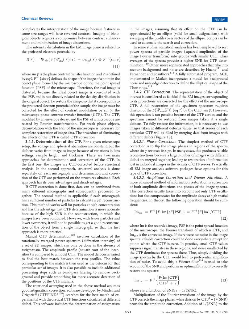
3.4.2. CTF Correction. The representation of the object ofinterest is considered as faithful if the EM images correspondingto its projections are corrected for the effects of the microscopeCTF. A full restoration of the specimen spectrum requiresdivision of the F{Ψsam(rB)} (eq 7) by the CTF, sin γ. However,this operation is not possible because of the CTF zeroes, and thespectrum cannot be restored from images taken at a singledefocus. To fully restore the information, it is necessary to useimages taken at different defocus values, so that zeroes of eachparticular CTF will be filled by merging data from images withdifferent defoci (Figure 13).3.4.2.1. Phase Correction. The simplest method of CTF
correction is to flip the image phases in regions of the spectrawhere sin γ reverses its sign. In many cases, this produces reliablereconstructions because a large number of images with differentdefoci are merged together, leading to restoration of informationlost in individual images in the vicinity of CTF zeroes. Practicallyall EM image analysis software packages have options for thistype of CTF correction.3.4.2.2. Amplitude Correction and Wiener Filtration. A
more advanced method of information restoration is correctionof both amplitude distortions and phases of the image spectra.This correction usually takes into account not only CTF oscilla-tions but also compensates for the amplitude decay at high spatialfrequencies. In theory, the following operation should be suffi-cient:
Imcor ¼ F�1fFfImg=FfPSFgg ¼ F�1fFfImg=CTFgð12Þ
where Im is the recorded image, PSF is the point spread functionof the microscope, the Fourier transform of which is CTF, andImcor is the corrected image. If there were no noise in the imagespectra, reliable correction could be done everywhere except forpoints where the CTF is zero. In practice, small CTF valuessuppress signal transfer in these regions, and noise unaffected bythe CTF dominates the spectra there. Thus, simply dividing theimage spectra by the CTF would lead to preferential amplifica-tion of noise. To avoid this, a Wiener filter114 is used to takeaccount of the SNR and perform an optimal filtration to correctlyrestore the spectra:
Imcor ¼ F�1 FfImgCTFCTF2 þ c
� �ð13Þ
where c is a function of SNR: c = 1/(SNR).Multiplication of the Fourier transform of the image by the
CTF corrects the image phases, while division by CTF2 + 1/(SNR)provides the amplitude correction. Addition of 1/(SNR) to the
7724 dx.doi.org/10.1021/cr100353t |Chem. Rev. 2011, 111, 7710–7748
Chemical Reviews REVIEW
denominator is necessary to avoid division by values close tozero115 (Figure 14). Amplitude correction has been implemen-ted in EMAN,116 SPIDER,117 Xmipp,118 and other softwarepackages. To visualize high-resolution details, it is also importantto correct the envelope decay of image amplitudes at high spatialfrequencies (see section 8.3).3.4.3. Image Normalization. After CTF correction, the
image of a weak phase object can be considered as a reasonableapproximation of the 2D projection of the 3D object, except forthe regions affected by CTF zeros, where the signal is low. Thisallows the process of image analysis to progress toward determi-nation of the 3D density distribution for the object. Nonetheless,some important steps of preprocessing are necessary.Even with the same EM settings during data acquisition,
variations in specimen particle orientation, support film thick-ness, and film processing conditions lead to differences in imagecontrast. In addition, structural analysis requires the merging ofimage data collected during multiple EM sessions. Optimizationof data processing requires standardization of images known asnormalization. It is conventional in EM image processing to setthe mean density of all particle images to the same level, usuallyzero, and to scale the standard deviation of the densities to thesame value for all images, which is important for the alignmentprocedure.Images are normalized using the formula:
Fnormi, j ¼ Fi, j � Fσold
σnew ð14Þ
σold is the standard deviation of the original image, and σnew is thetarget standard deviation in the data.The mean density of the images is defined as
F ¼∑I, J
i, j¼ 1Fi, j
I � Jð15Þ
where I and J are dimensions of the image array, and Fi,j isthe density in the image pixel with coordinates i and j. σold isdefined as
σold ¼
ffiffiffiffiffiffiffiffiffiffiffiffiffiffiffiffiffiffiffiffiffiffiffiffiffiffiffiffiffiffiffiffiffi∑I, J
i, j¼ 1ðFi, j � FÞ2
ðI � 1Þ � ðJ � 1Þ
vuuuut ð16Þ
The normalization sets all images to the same standard deviationand a mean density of zero.
4. IMAGE ALIGNMENT
The information we wish to extract from EM images, thesignal, is the projected density of the structure of interest. Therecorded images contain, in addition to the signal, fluctuations inintensity caused by noise frommany different sources. Sources ofnoise include background variations in ice or stain, damage to themolecule from preparation procedures or radiation, and detector
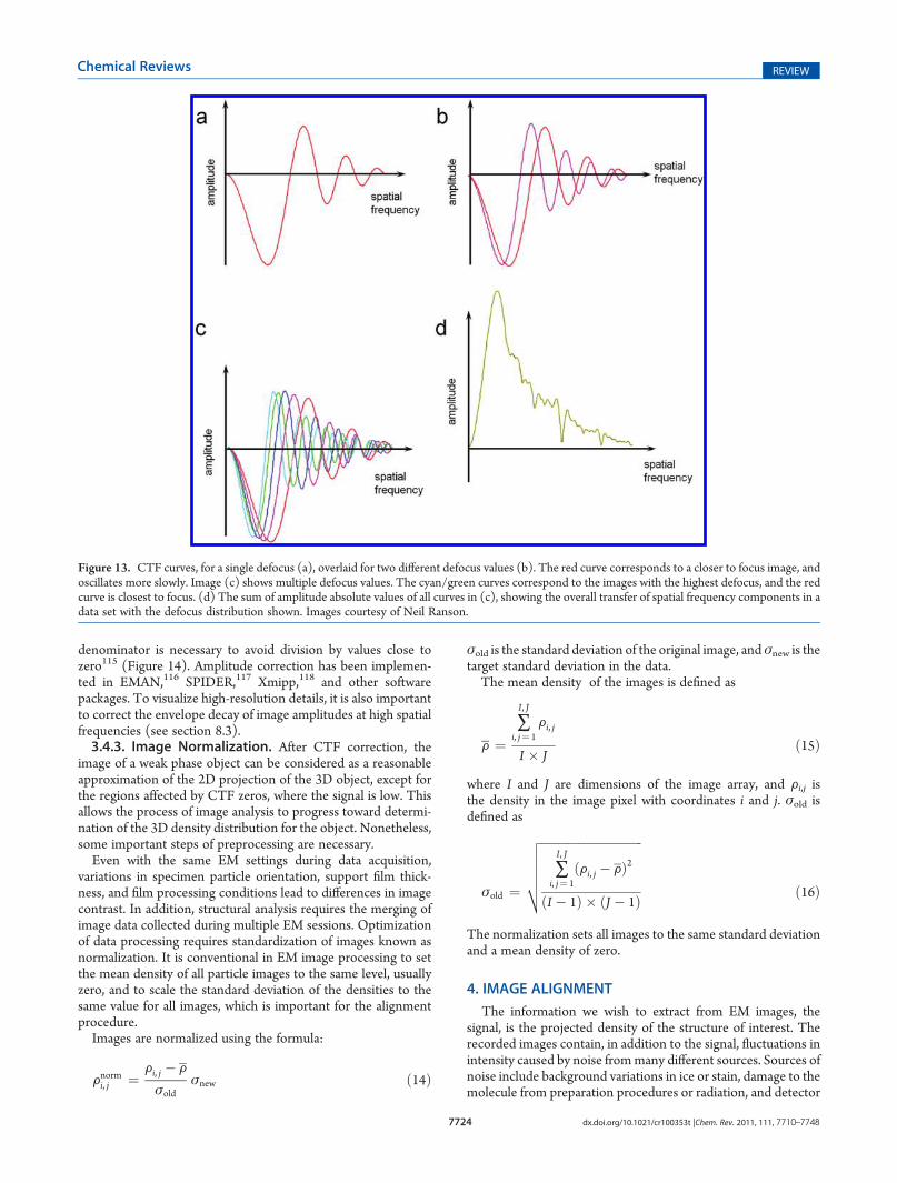
Figure 13. CTF curves, for a single defocus (a), overlaid for two different defocus values (b). The red curve corresponds to a closer to focus image, andoscillates more slowly. Image (c) shows multiple defocus values. The cyan/green curves correspond to the images with the highest defocus, and the redcurve is closest to focus. (d) The sum of amplitude absolute values of all curves in (c), showing the overall transfer of spatial frequency components in adata set with the defocus distribution shown. Images courtesy of Neil Ranson.
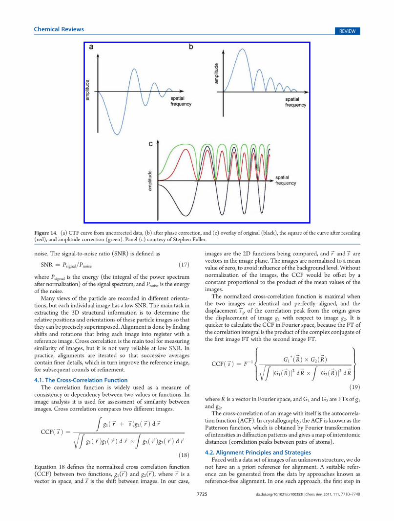
7725 dx.doi.org/10.1021/cr100353t |Chem. Rev. 2011, 111, 7710–7748
Chemical Reviews REVIEW
noise. The signal-to-noise ratio (SNR) is defined as
SNR ¼ Psignal=Pnoise ð17Þwhere Psignal is the energy (the integral of the power spectrumafter normalization) of the signal spectrum, and Pnoise is the energyof the noise.
Many views of the particle are recorded in different orienta-tions, but each individual image has a low SNR. The main task inextracting the 3D structural information is to determine therelative positions and orientations of these particle images so thatthey can be precisely superimposed. Alignment is done by findingshifts and rotations that bring each image into register with areference image. Cross correlation is the main tool for measuringsimilarity of images, but it is not very reliable at low SNR. Inpractice, alignments are iterated so that successive averagescontain finer details, which in turn improve the reference image,for subsequent rounds of refinement.
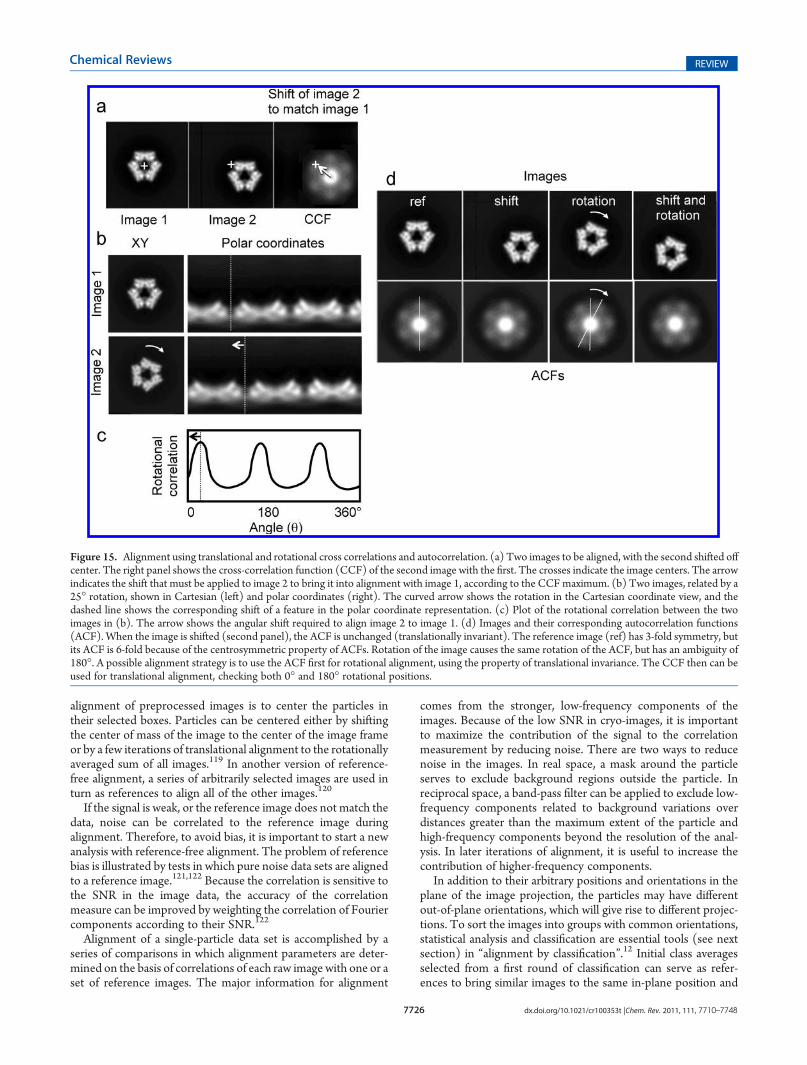
4.1. The Cross-Correlation FunctionThe correlation function is widely used as a measure of
consistency or dependency between two values or functions. Inimage analysis it is used for assessment of similarity betweenimages. Cross correlation compares two different images.
CCFð sBÞ ¼
Zg1ð rB þ sBÞg2ð rBÞ d rBffiffiffiffiffiffiffiffiffiffiffiffiffiffiffiffiffiffiffiffiffiffiffiffiffiffiffiffiffiffiffiffiffiffiffiffiffiffiffiffiffiffiffiffiffiffiffiffiffiffiffiffiffiffiffiffiffiffiffiffiffiffiffiffiffiffiffiffiffiffiffiffiffiffiffiffiffiffiZ
g1ð rBÞg1ð rBÞ d rB�Z
g2ð rBÞg2ð rBÞ d rB
r
ð18ÞEquation 18 defines the normalized cross correlation function(CCF) between two functions, g1(rB) and g2(rB), where rB is avector in space, and sB is the shift between images. In our case,
images are the 2D functions being compared, and rB and sB arevectors in the image plane. The images are normalized to a meanvalue of zero, to avoid influence of the background level. Withoutnormalization of the images, the CCF would be offset by aconstant proportional to the product of the mean values of theimages.
The normalized cross-correlation function is maximal whenthe two images are identical and perfectly aligned, and thedisplacement sBp of the correlation peak from the origin givesthe displacement of image g1 with respect to image g2. It isquicker to calculate the CCF in Fourier space, because the FT ofthe correlation integral is the product of the complex conjugate ofthe first image FT with the second image FT.
CCFð sBÞ ¼ F�1 G1�ðRBÞ � G2ðRBÞffiffiffiffiffiffiffiffiffiffiffiffiffiffiffiffiffiffiffiffiffiffiffiffiffiffiffiffiffiffiffiffiffiffiffiffiffiffiffiffiffiffiffiffiffiffiffiffiffiffiffiffiffiffiffiffiffiffiffiffiffiffiffiffiZ
jG1ðRBÞj2 dRB�Z
jG2ðRBÞj2 dRBr
8>>><>>>:
9>>>=>>>;ð19Þ
where RB is a vector in Fourier space, and G1 and G2 are FTs of g1and g2.
The cross-correlation of an image with itself is the autocorrela-tion function (ACF). In crystallography, the ACF is known as thePatterson function, which is obtained by Fourier transformationof intensities in diffraction patterns and gives amap of interatomicdistances (correlation peaks between pairs of atoms).
4.2. Alignment Principles and StrategiesFaced with a data set of images of an unknown structure, we do
not have an a priori reference for alignment. A suitable refer-ence can be generated from the data by approaches known asreference-free alignment. In one such approach, the first step in
Figure 14. (a) CTF curve from uncorrected data, (b) after phase correction, and (c) overlay of original (black), the square of the curve after rescaling(red), and amplitude correction (green). Panel (c) courtesy of Stephen Fuller.
7726 dx.doi.org/10.1021/cr100353t |Chem. Rev. 2011, 111, 7710–7748
Chemical Reviews REVIEW
alignment of preprocessed images is to center the particles intheir selected boxes. Particles can be centered either by shiftingthe center of mass of the image to the center of the image frameor by a few iterations of translational alignment to the rotationallyaveraged sum of all images.119 In another version of reference-free alignment, a series of arbitrarily selected images are used inturn as references to align all of the other images.120
If the signal is weak, or the reference image does not match thedata, noise can be correlated to the reference image duringalignment. Therefore, to avoid bias, it is important to start a newanalysis with reference-free alignment. The problem of referencebias is illustrated by tests in which pure noise data sets are alignedto a reference image.121,122 Because the correlation is sensitive tothe SNR in the image data, the accuracy of the correlationmeasure can be improved by weighting the correlation of Fouriercomponents according to their SNR.122
Alignment of a single-particle data set is accomplished by aseries of comparisons in which alignment parameters are deter-mined on the basis of correlations of each raw image with one or aset of reference images. The major information for alignment
comes from the stronger, low-frequency components of theimages. Because of the low SNR in cryo-images, it is importantto maximize the contribution of the signal to the correlationmeasurement by reducing noise. There are two ways to reducenoise in the images. In real space, a mask around the particleserves to exclude background regions outside the particle. Inreciprocal space, a band-pass filter can be applied to exclude low-frequency components related to background variations overdistances greater than the maximum extent of the particle andhigh-frequency components beyond the resolution of the anal-ysis. In later iterations of alignment, it is useful to increase thecontribution of higher-frequency components.
In addition to their arbitrary positions and orientations in theplane of the image projection, the particles may have differentout-of-plane orientations, which will give rise to different projec-tions. To sort the images into groups with common orientations,statistical analysis and classification are essential tools (see nextsection) in “alignment by classification”.12 Initial class averagesselected from a first round of classification can serve as refer-ences to bring similar images to the same in-plane position and
Figure 15. Alignment using translational and rotational cross correlations and autocorrelation. (a) Two images to be aligned, with the second shifted offcenter. The right panel shows the cross-correlation function (CCF) of the second image with the first. The crosses indicate the image centers. The arrowindicates the shift that must be applied to image 2 to bring it into alignment with image 1, according to the CCFmaximum. (b) Two images, related by a25� rotation, shown in Cartesian (left) and polar coordinates (right). The curved arrow shows the rotation in the Cartesian coordinate view, and thedashed line shows the corresponding shift of a feature in the polar coordinate representation. (c) Plot of the rotational correlation between the twoimages in (b). The arrow shows the angular shift required to align image 2 to image 1. (d) Images and their corresponding autocorrelation functions(ACF). When the image is shifted (second panel), the ACF is unchanged (translationally invariant). The reference image (ref) has 3-fold symmetry, butits ACF is 6-fold because of the centrosymmetric property of ACFs. Rotation of the image causes the same rotation of the ACF, but has an ambiguity of180�. A possible alignment strategy is to use the ACF first for rotational alignment, using the property of translational invariance. The CCF then can beused for translational alignment, checking both 0� and 180� rotational positions.
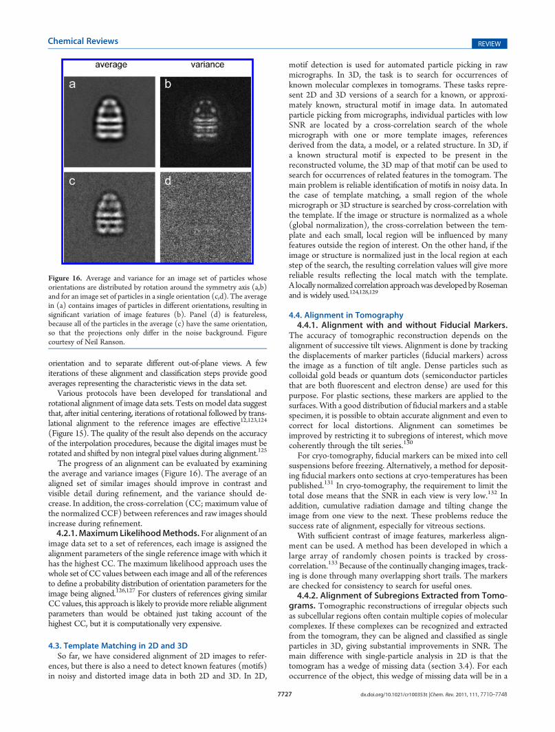
7727 dx.doi.org/10.1021/cr100353t |Chem. Rev. 2011, 111, 7710–7748
Chemical Reviews REVIEW
orientation and to separate different out-of-plane views. A fewiterations of these alignment and classification steps provide goodaverages representing the characteristic views in the data set.
Various protocols have been developed for translational androtational alignment of image data sets. Tests onmodel data suggestthat, after initial centering, iterations of rotational followed by trans-lational alignment to the reference images are effective12,123,124
(Figure 15). The quality of the result also depends on the accuracyof the interpolation procedures, because the digital images must berotated and shifted by non integral pixel values during alignment.125
The progress of an alignment can be evaluated by examiningthe average and variance images (Figure 16). The average of analigned set of similar images should improve in contrast andvisible detail during refinement, and the variance should de-crease. In addition, the cross-correlation (CC; maximum value ofthe normalized CCF) between references and raw images shouldincrease during refinement.4.2.1.MaximumLikelihoodMethods. For alignment of an
image data set to a set of references, each image is assigned thealignment parameters of the single reference image with which ithas the highest CC. The maximum likelihood approach uses thewhole set of CC values between each image and all of the referencesto define a probability distribution of orientation parameters for theimage being aligned.126,127 For clusters of references giving similarCC values, this approach is likely to providemore reliable alignmentparameters than would be obtained just taking account of thehighest CC, but it is computationally very expensive.
4.3. Template Matching in 2D and 3DSo far, we have considered alignment of 2D images to refer-
ences, but there is also a need to detect known features (motifs)in noisy and distorted image data in both 2D and 3D. In 2D,
motif detection is used for automated particle picking in rawmicrographs. In 3D, the task is to search for occurrences ofknown molecular complexes in tomograms. These tasks repre-sent 2D and 3D versions of a search for a known, or approxi-mately known, structural motif in image data. In automatedparticle picking from micrographs, individual particles with lowSNR are located by a cross-correlation search of the wholemicrograph with one or more template images, referencesderived from the data, a model, or a related structure. In 3D, ifa known structural motif is expected to be present in thereconstructed volume, the 3D map of that motif can be used tosearch for occurrences of related features in the tomogram. Themain problem is reliable identification of motifs in noisy data. Inthe case of template matching, a small region of the wholemicrograph or 3D structure is searched by cross-correlation withthe template. If the image or structure is normalized as a whole(global normalization), the cross-correlation between the tem-plate and each small, local region will be influenced by manyfeatures outside the region of interest. On the other hand, if theimage or structure is normalized just in the local region at eachstep of the search, the resulting correlation values will give morereliable results reflecting the local match with the template.A locally normalized correlation approachwasdevelopedbyRosemanand is widely used.124,128,129
4.4. Alignment in Tomography4.4.1. Alignment with and without Fiducial Markers.
The accuracy of tomographic reconstruction depends on thealignment of successive tilt views. Alignment is done by trackingthe displacements of marker particles (fiducial markers) acrossthe image as a function of tilt angle. Dense particles such ascolloidal gold beads or quantum dots (semiconductor particlesthat are both fluorescent and electron dense) are used for thispurpose. For plastic sections, these markers are applied to thesurfaces. With a good distribution of fiducial markers and a stablespecimen, it is possible to obtain accurate alignment and even tocorrect for local distortions. Alignment can sometimes beimproved by restricting it to subregions of interest, which movecoherently through the tilt series.130
For cryo-tomography, fiducial markers can be mixed into cellsuspensions before freezing. Alternatively, a method for deposit-ing fiducial markers onto sections at cryo-temperatures has beenpublished.131 In cryo-tomography, the requirement to limit thetotal dose means that the SNR in each view is very low.132 Inaddition, cumulative radiation damage and tilting change theimage from one view to the next. These problems reduce thesuccess rate of alignment, especially for vitreous sections.With sufficient contrast of image features, markerless align-
ment can be used. A method has been developed in which alarge array of randomly chosen points is tracked by cross-correlation.133 Because of the continually changing images, track-ing is done through many overlapping short trails. The markersare checked for consistency to search for useful ones.4.4.2. Alignment of Subregions Extracted from Tomo-
grams. Tomographic reconstructions of irregular objects suchas subcellular regions often contain multiple copies of molecularcomplexes. If these complexes can be recognized and extractedfrom the tomogram, they can be aligned and classified as singleparticles in 3D, giving substantial improvements in SNR. Themain difference with single-particle analysis in 2D is that thetomogram has a wedge of missing data (section 3.4). For eachoccurrence of the object, this wedge of missing data will be in a
Figure 16. Average and variance for an image set of particles whoseorientations are distributed by rotation around the symmetry axis (a,b)and for an image set of particles in a single orientation (c,d). The averagein (a) contains images of particles in different orientations, resulting insignificant variation of image features (b). Panel (d) is featureless,because all of the particles in the average (c) have the same orientation,so that the projections only differ in the noise background. Figurecourtesy of Neil Ranson.
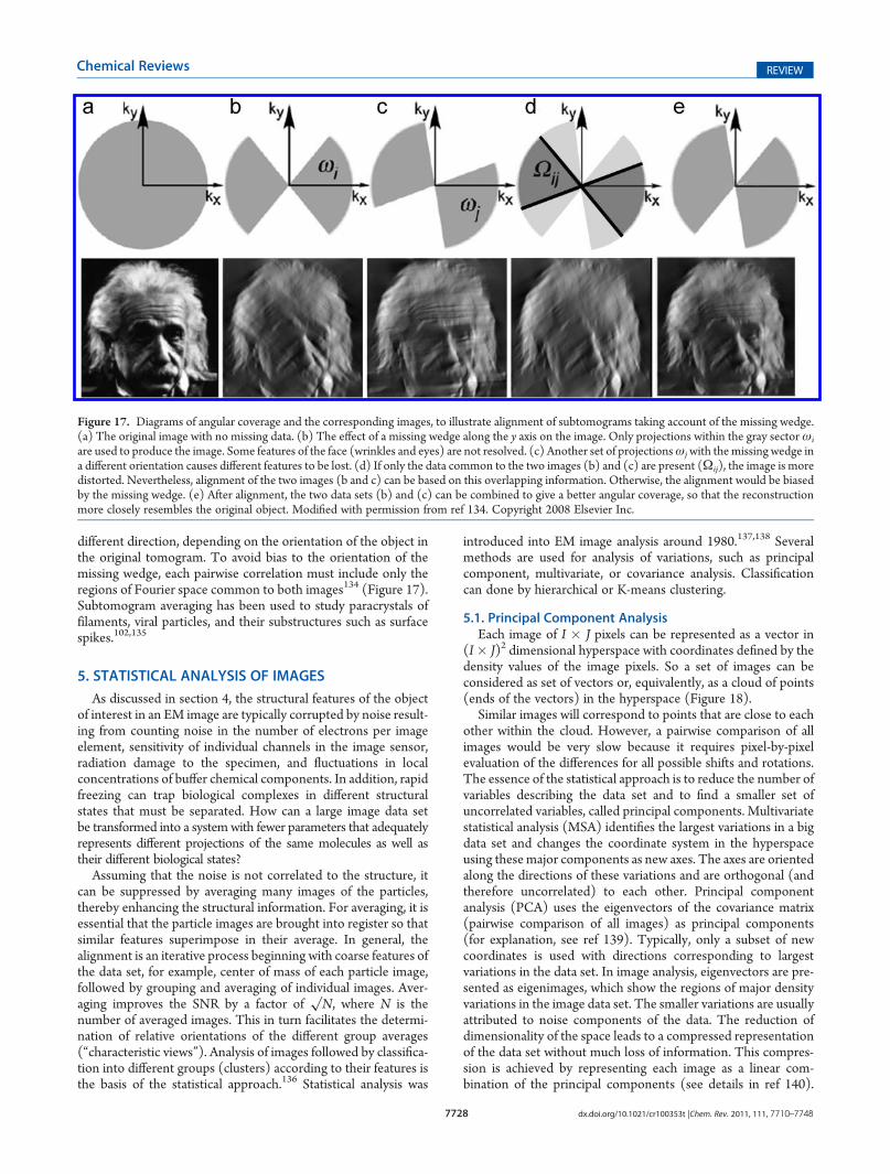
7728 dx.doi.org/10.1021/cr100353t |Chem. Rev. 2011, 111, 7710–7748
Chemical Reviews REVIEW
different direction, depending on the orientation of the object inthe original tomogram. To avoid bias to the orientation of themissing wedge, each pairwise correlation must include only theregions of Fourier space common to both images134 (Figure 17).Subtomogram averaging has been used to study paracrystals offilaments, viral particles, and their substructures such as surfacespikes.102,135
5. STATISTICAL ANALYSIS OF IMAGES
As discussed in section 4, the structural features of the objectof interest in an EM image are typically corrupted by noise result-ing from counting noise in the number of electrons per imageelement, sensitivity of individual channels in the image sensor,radiation damage to the specimen, and fluctuations in localconcentrations of buffer chemical components. In addition, rapidfreezing can trap biological complexes in different structuralstates that must be separated. How can a large image data setbe transformed into a systemwith fewer parameters that adequatelyrepresents different projections of the same molecules as well astheir different biological states?
Assuming that the noise is not correlated to the structure, itcan be suppressed by averaging many images of the particles,thereby enhancing the structural information. For averaging, it isessential that the particle images are brought into register so thatsimilar features superimpose in their average. In general, thealignment is an iterative process beginning with coarse features ofthe data set, for example, center of mass of each particle image,followed by grouping and averaging of individual images. Aver-aging improves the SNR by a factor of
√N, where N is the
number of averaged images. This in turn facilitates the determi-nation of relative orientations of the different group averages(“characteristic views”). Analysis of images followed by classifica-tion into different groups (clusters) according to their features isthe basis of the statistical approach.136 Statistical analysis was
introduced into EM image analysis around 1980.137,138 Severalmethods are used for analysis of variations, such as principalcomponent, multivariate, or covariance analysis. Classificationcan done by hierarchical or K-means clustering.
5.1. Principal Component AnalysisEach image of I � J pixels can be represented as a vector in
(I� J)2 dimensional hyperspace with coordinates defined by thedensity values of the image pixels. So a set of images can beconsidered as set of vectors or, equivalently, as a cloud of points(ends of the vectors) in the hyperspace (Figure 18).
Similar images will correspond to points that are close to eachother within the cloud. However, a pairwise comparison of allimages would be very slow because it requires pixel-by-pixelevaluation of the differences for all possible shifts and rotations.The essence of the statistical approach is to reduce the number ofvariables describing the data set and to find a smaller set ofuncorrelated variables, called principal components. Multivariatestatistical analysis (MSA) identifies the largest variations in a bigdata set and changes the coordinate system in the hyperspaceusing thesemajor components as new axes. The axes are orientedalong the directions of these variations and are orthogonal (andtherefore uncorrelated) to each other. Principal componentanalysis (PCA) uses the eigenvectors of the covariance matrix(pairwise comparison of all images) as principal components(for explanation, see ref 139). Typically, only a subset of newcoordinates is used with directions corresponding to largestvariations in the data set. In image analysis, eigenvectors are pre-sented as eigenimages, which show the regions of major densityvariations in the image data set. The smaller variations are usuallyattributed to noise components of the data. The reduction ofdimensionality of the space leads to a compressed representationof the data set without much loss of information. This compres-sion is achieved by representing each image as a linear com-bination of the principal components (see details in ref 140).
Figure 17. Diagrams of angular coverage and the corresponding images, to illustrate alignment of subtomograms taking account of the missing wedge.(a) The original image with no missing data. (b) The effect of a missing wedge along the y axis on the image. Only projections within the gray sectorωi
are used to produce the image. Some features of the face (wrinkles and eyes) are not resolved. (c) Another set of projectionsωjwith themissing wedge ina different orientation causes different features to be lost. (d) If only the data common to the two images (b) and (c) are present (Ωij), the image is moredistorted. Nevertheless, alignment of the two images (b and c) can be based on this overlapping information. Otherwise, the alignment would be biasedby the missing wedge. (e) After alignment, the two data sets (b) and (c) can be combined to give a better angular coverage, so that the reconstructionmore closely resembles the original object. Modified with permission from ref 134. Copyright 2008 Elsevier Inc.
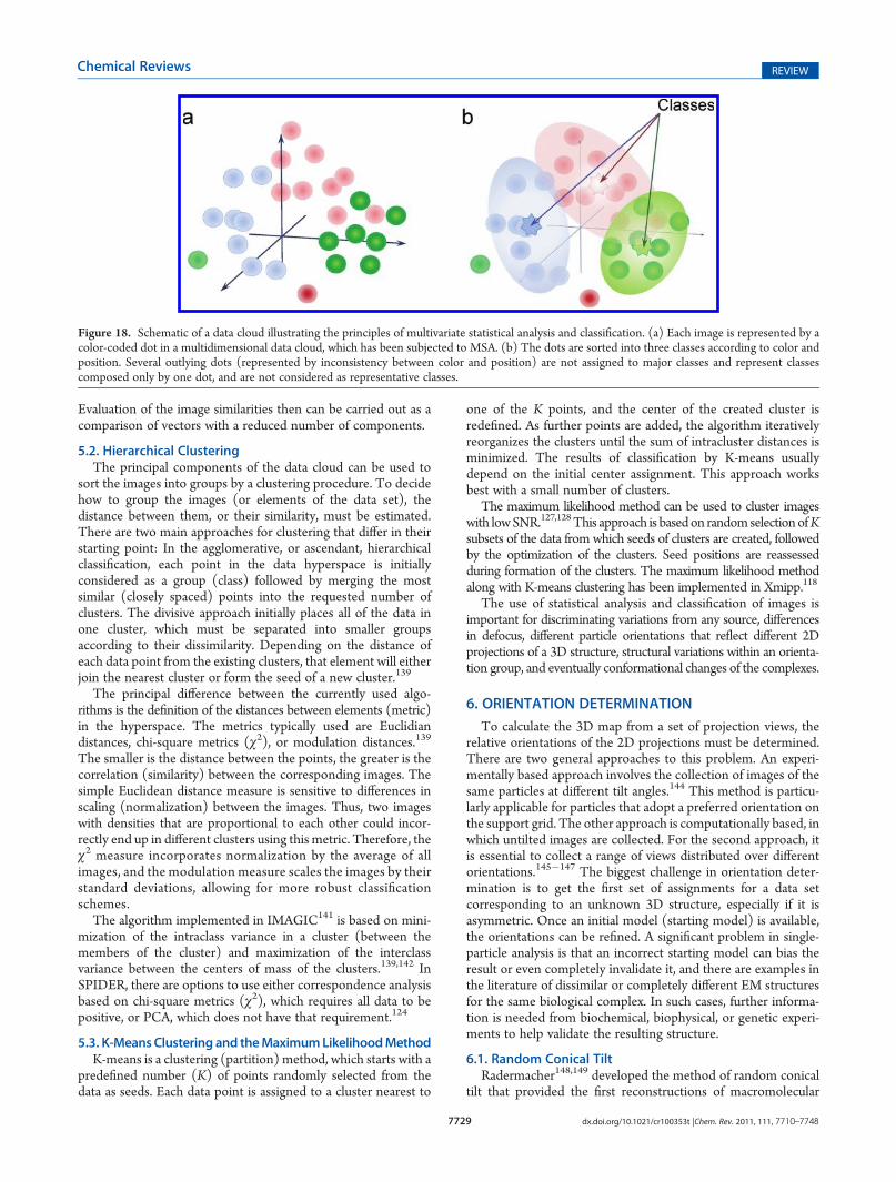
7729 dx.doi.org/10.1021/cr100353t |Chem. Rev. 2011, 111, 7710–7748
Chemical Reviews REVIEW
Evaluation of the image similarities then can be carried out as acomparison of vectors with a reduced number of components.
5.2. Hierarchical ClusteringThe principal components of the data cloud can be used to
sort the images into groups by a clustering procedure. To decidehow to group the images (or elements of the data set), thedistance between them, or their similarity, must be estimated.There are two main approaches for clustering that differ in theirstarting point: In the agglomerative, or ascendant, hierarchicalclassification, each point in the data hyperspace is initiallyconsidered as a group (class) followed by merging the mostsimilar (closely spaced) points into the requested number ofclusters. The divisive approach initially places all of the data inone cluster, which must be separated into smaller groupsaccording to their dissimilarity. Depending on the distance ofeach data point from the existing clusters, that element will eitherjoin the nearest cluster or form the seed of a new cluster.139
The principal difference between the currently used algo-rithms is the definition of the distances between elements (metric)in the hyperspace. The metrics typically used are Euclidiandistances, chi-square metrics (χ2), or modulation distances.139
The smaller is the distance between the points, the greater is thecorrelation (similarity) between the corresponding images. Thesimple Euclidean distance measure is sensitive to differences inscaling (normalization) between the images. Thus, two imageswith densities that are proportional to each other could incor-rectly end up in different clusters using this metric. Therefore, theχ2 measure incorporates normalization by the average of allimages, and the modulation measure scales the images by theirstandard deviations, allowing for more robust classificationschemes.
The algorithm implemented in IMAGIC141 is based on mini-mization of the intraclass variance in a cluster (between themembers of the cluster) and maximization of the interclassvariance between the centers of mass of the clusters.139,142 InSPIDER, there are options to use either correspondence analysisbased on chi-square metrics (χ2), which requires all data to bepositive, or PCA, which does not have that requirement.124
5.3. K-MeansClustering and theMaximumLikelihoodMethodK-means is a clustering (partition) method, which starts with a
predefined number (K) of points randomly selected from thedata as seeds. Each data point is assigned to a cluster nearest to
one of the K points, and the center of the created cluster isredefined. As further points are added, the algorithm iterativelyreorganizes the clusters until the sum of intracluster distances isminimized. The results of classification by K-means usuallydepend on the initial center assignment. This approach worksbest with a small number of clusters.
The maximum likelihood method can be used to cluster imageswith lowSNR.127,128This approach is basedon randomselectionofKsubsets of the data from which seeds of clusters are created, followedby the optimization of the clusters. Seed positions are reassessedduring formation of the clusters. The maximum likelihood methodalong with K-means clustering has been implemented in Xmipp.118
The use of statistical analysis and classification of images isimportant for discriminating variations from any source, differencesin defocus, different particle orientations that reflect different 2Dprojections of a 3D structure, structural variations within an orienta-tion group, and eventually conformational changes of the complexes.
6. ORIENTATION DETERMINATION
To calculate the 3D map from a set of projection views, therelative orientations of the 2D projections must be determined.There are two general approaches to this problem. An experi-mentally based approach involves the collection of images of thesame particles at different tilt angles.144 This method is particu-larly applicable for particles that adopt a preferred orientation onthe support grid. The other approach is computationally based, inwhich untilted images are collected. For the second approach, itis essential to collect a range of views distributed over differentorientations.145�147 The biggest challenge in orientation deter-mination is to get the first set of assignments for a data setcorresponding to an unknown 3D structure, especially if it isasymmetric. Once an initial model (starting model) is available,the orientations can be refined. A significant problem in single-particle analysis is that an incorrect starting model can bias theresult or even completely invalidate it, and there are examples inthe literature of dissimilar or completely different EM structuresfor the same biological complex. In such cases, further informa-tion is needed from biochemical, biophysical, or genetic experi-ments to help validate the resulting structure.
6.1. Random Conical TiltRadermacher148,149 developed the method of random conical
tilt that provided the first reconstructions of macromolecular
Figure 18. Schematic of a data cloud illustrating the principles of multivariate statistical analysis and classification. (a) Each image is represented by acolor-coded dot in a multidimensional data cloud, which has been subjected to MSA. (b) The dots are sorted into three classes according to color andposition. Several outlying dots (represented by inconsistency between color and position) are not assigned to major classes and represent classescomposed only by one dot, and are not considered as representative classes.
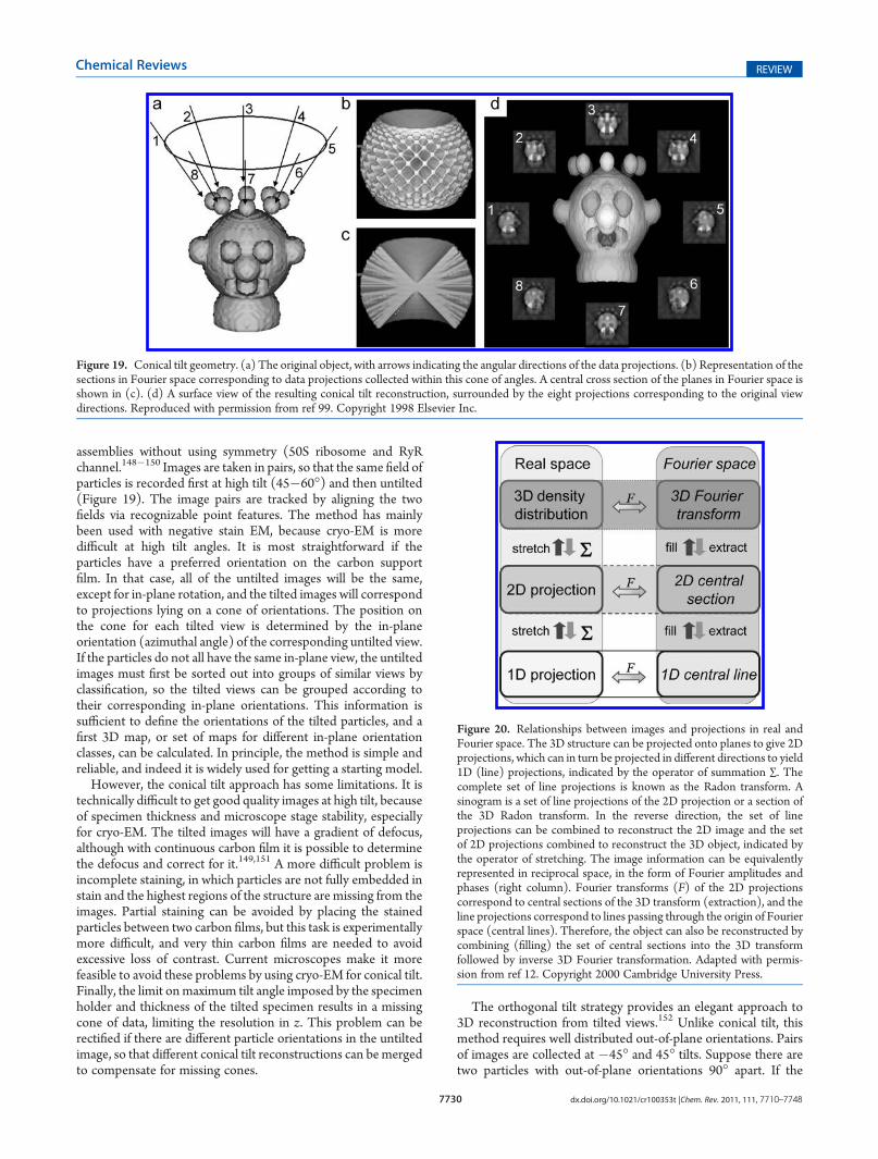
7730 dx.doi.org/10.1021/cr100353t |Chem. Rev. 2011, 111, 7710–7748
Chemical Reviews REVIEW
assemblies without using symmetry (50S ribosome and RyRchannel.148�150 Images are taken in pairs, so that the same field ofparticles is recorded first at high tilt (45�60�) and then untilted(Figure 19). The image pairs are tracked by aligning the twofields via recognizable point features. The method has mainlybeen used with negative stain EM, because cryo-EM is moredifficult at high tilt angles. It is most straightforward if theparticles have a preferred orientation on the carbon supportfilm. In that case, all of the untilted images will be the same,except for in-plane rotation, and the tilted images will correspondto projections lying on a cone of orientations. The position onthe cone for each tilted view is determined by the in-planeorientation (azimuthal angle) of the corresponding untilted view.If the particles do not all have the same in-plane view, the untiltedimages must first be sorted out into groups of similar views byclassification, so the tilted views can be grouped according totheir corresponding in-plane orientations. This information issufficient to define the orientations of the tilted particles, and afirst 3D map, or set of maps for different in-plane orientationclasses, can be calculated. In principle, the method is simple andreliable, and indeed it is widely used for getting a starting model.
However, the conical tilt approach has some limitations. It istechnically difficult to get good quality images at high tilt, becauseof specimen thickness and microscope stage stability, especiallyfor cryo-EM. The tilted images will have a gradient of defocus,although with continuous carbon film it is possible to determinethe defocus and correct for it.149,151 A more difficult problem isincomplete staining, in which particles are not fully embedded instain and the highest regions of the structure are missing from theimages. Partial staining can be avoided by placing the stainedparticles between two carbon films, but this task is experimentallymore difficult, and very thin carbon films are needed to avoidexcessive loss of contrast. Current microscopes make it morefeasible to avoid these problems by using cryo-EM for conical tilt.Finally, the limit onmaximum tilt angle imposed by the specimenholder and thickness of the tilted specimen results in a missingcone of data, limiting the resolution in z. This problem can berectified if there are different particle orientations in the untiltedimage, so that different conical tilt reconstructions can bemergedto compensate for missing cones.
The orthogonal tilt strategy provides an elegant approach to3D reconstruction from tilted views.152 Unlike conical tilt, thismethod requires well distributed out-of-plane orientations. Pairsof images are collected at �45� and 45� tilts. Suppose there aretwo particles with out-of-plane orientations 90� apart. If the
Figure 19. Conical tilt geometry. (a) The original object, with arrows indicating the angular directions of the data projections. (b) Representation of thesections in Fourier space corresponding to data projections collected within this cone of angles. A central cross section of the planes in Fourier space isshown in (c). (d) A surface view of the resulting conical tilt reconstruction, surrounded by the eight projections corresponding to the original viewdirections. Reproduced with permission from ref 99. Copyright 1998 Elsevier Inc.
Figure 20. Relationships between images and projections in real andFourier space. The 3D structure can be projected onto planes to give 2Dprojections, which can in turn be projected in different directions to yield1D (line) projections, indicated by the operator of summation ∑. Thecomplete set of line projections is known as the Radon transform. Asinogram is a set of line projections of the 2D projection or a section ofthe 3D Radon transform. In the reverse direction, the set of lineprojections can be combined to reconstruct the 2D image and the setof 2D projections combined to reconstruct the 3D object, indicated bythe operator of stretching. The image information can be equivalentlyrepresented in reciprocal space, in the form of Fourier amplitudes andphases (right column). Fourier transforms (F) of the 2D projectionscorrespond to central sections of the 3D transform (extraction), and theline projections correspond to lines passing through the origin of Fourierspace (central lines). Therefore, the object can also be reconstructed bycombining (filling) the set of central sections into the 3D transformfollowed by inverse 3D Fourier transformation. Adapted with permis-sion from ref 12. Copyright 2000 Cambridge University Press.
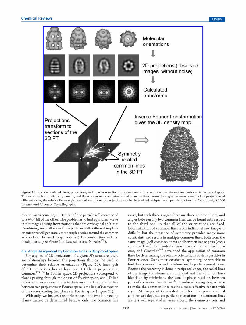
7731 dx.doi.org/10.1021/cr100353t |Chem. Rev. 2011, 111, 7710–7748
Chemical Reviews REVIEW
rotation axes coincide, a�45� tilt of one particle will correspondto a +45� tilt of the other. The problem is to find equivalent viewsin tilt images arising from particles that are orthogonal at 0� tilt.Combining such tilt views from particles with different in-planeorientations will generate a tomographic series around the commonaxis and can be used to generate a 3D reconstruction with nomissing cone (see Figure 1 of Leschziner and Nogales152).
6.2. Angle Assignment by Common Lines in Reciprocal SpaceFor any set of 2D projections of a given 3D structure, there
are relationships between the projections that can be used todetermine their relative orientations (Figure 20). Each pairof 2D projections has at least one 1D (line) projection incommon.153,154 In Fourier space, 2D projections correspond toplanes passing through the origin of Fourier space, and 1D lineprojections become radial lines in the transform.The common linebetween two projections in Fourier space is the line of intersectionof the corresponding two planes in Fourier space (Figure 21).
With only two images, the angle between the two intersectingplanes cannot be determined because only one common line
exists, but with three images there are three common lines, andangles between any two common lines can be found with respectto the third one, so that all of the orientations are fixed.Determination of common lines from individual raw images isdifficult, but the presence of symmetry provides many moreconstraints and results in multiple common lines, both from thesame image (self-common lines) and between image pairs (crosscommon lines). Icosahedral viruses provide the most favorablecase, and Crowther145 developed the application of commonlines for determining the relative orientations of virus particles inFourier space. Using their icosahedral symmetry, he was able tofind the common lines and to determine the particle orientations.Because the searching is done in reciprocal space, the radial linesof the image transforms are compared and the common linesidentified by minimizing the sum of phase residuals betweenpairs of common lines. Fuller155 introduced a weighting schemeto make the common lines method more effective for use withcryo EM images of icosahedral particles. The phase residualcomparison depends on particle orientation: the common linesare less well separated in views around the symmetry axes, and
Figure 21. Surface rendered views, projections, and transform sections of a structure, with a common line intersection illustrated in reciprocal space.The structure has rotational symmetry, and there are several symmetry-related common lines. From the angles between common line projections ofdifferent views, the relative Euler-angle orientations of a set of projections can be determined. Adapted with permission from ref 24. Copyright 2000International Union of Crystallography.
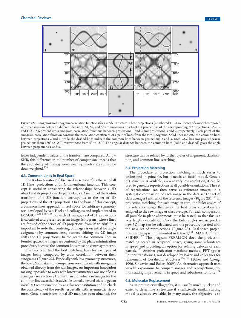
7732 dx.doi.org/10.1021/cr100353t |Chem. Rev. 2011, 111, 7710–7748
Chemical Reviews REVIEW
fewer independent values of the transform are compared. At lowSNR, this difference in the number of comparisons means thatthe probability of finding views near symmetry axes must bedownweighted.156
6.3. Common Lines in Real SpaceThe Radon transform (discussed in section 7) is the set of all
1D (line) projections of an N-dimensional function. This con-cept is useful in considering the relationships between a 3Dobject and its projections. In particular, a 2D section of the Radontransform of a 3D function corresponds to the set of 1Dprojections of the 2D projection. On the basis of this concept,a common lines approach in real space for arbitrary symmetrywas developed by van Heel and colleagues and implemented inIMAGIC.12,154,157,158 For each 2D image, a set of 1D projectionsis calculated and presented as an image (sinogram) whose linesare formed of the series of 1D projections from 0� to 360�. It isimportant to note that centering of images is essential for angleassignment by common lines, because shifting the 2D imageshifts the 1D projections. In the search for common lines inFourier space, the images are centered by the phase minimizationprocedure, because the common lines must be centrosymmetric.
The task is to find the best matching lines for each pair ofimages being compared, by cross correlation between theirsinograms (Figure 22). Especially with low symmetry structures,the low SNRmakes this comparison very difficult with sinogramsobtained directly from the raw images. An important innovationmaking it possible to work with lower symmetries was use of classaverages (see section 5) rather than individual raw images for thecommon lines search. It is advisible tomake several trials to get aninitial 3D reconstruction by angular reconstitution and to checkthe consistency of the results, especially with asymmetric struc-tures. Once a consistent initial 3D map has been obtained, the
structure can be refined by further cycles of alignment, classifica-tion, and common line searching.
6.4. Projection MatchingThe procedure of projection matching is much easier to
understand in principle, but it needs an initial model. Once a3D structure is available, even at very low resolution, it can beused to generate reprojections at all possible orientations. The setof reprojections can then serve as reference images, in asystematic comparison of each image in the data set (or set ofclass averages) with all of the reference images (Figure 23).159 Inprojection matching, for each image in turn, the Euler angles ofthe reference image that gives the best cross correlation areassigned to the raw image or class average. For each comparison,all possible in-plane alignments must be tested, so that this is avery lengthy calculation. Once the Euler angles are assigned, anew 3D map can be calculated and the procedure iterated withthe new set of reprojections (Figure 23). Real-space projec-tion matching is implemented in EMAN,116 IMAGIC,141 andSPIDER.117 The program FREALIGN does the projectionmatching search in reciprocal space, giving some advantagesin speed and providing an option for refining defocus of eachparticle.160 Another projection matching method, PFT (polarFourier transforms), was developed by Baker and colleagues forrefinement of icosahedral structures146,161 (Baker and Cheng,1996, Sinkovits and Baker, 2009). An alternative approach useswavelet expansions to compare images and reprojections, de-monstrating improvements in speed and robustness to noise.162
6.5. Molecular ReplacementAs in protein crystallography, it is usually much quicker and
easier to determine a structure if a sufficiently similar startingmodel is already available. In many cases, the objective is to
Figure 22. Sinograms and sinogram correlation functions for a model structure. Three projections (numbered 1�3) are shown of a model composedof three Gaussian dots with different densities. S1, S2, and S3 are sinograms or sets of 1D projections of the corresponding 2D projections. CSC12and CSC32 represent cross-sinogram correlation functions between projections 1 and 2 and projections 3 and 2, respectively. Each point of thesinogram correlation function contains the correlation coefficient of a pair of lines from the two sinograms. Solid lines indicate the common linesbetween projections 2 and 1, while the dashed lines indicate the common lines between projections 2 and 3. Each CSC has two peaks becauseprojections from 180� to 360� mirror those from 0� to 180�. The angular distance between the common lines (solid and dashed) gives the anglebetween projections 1 and 3.
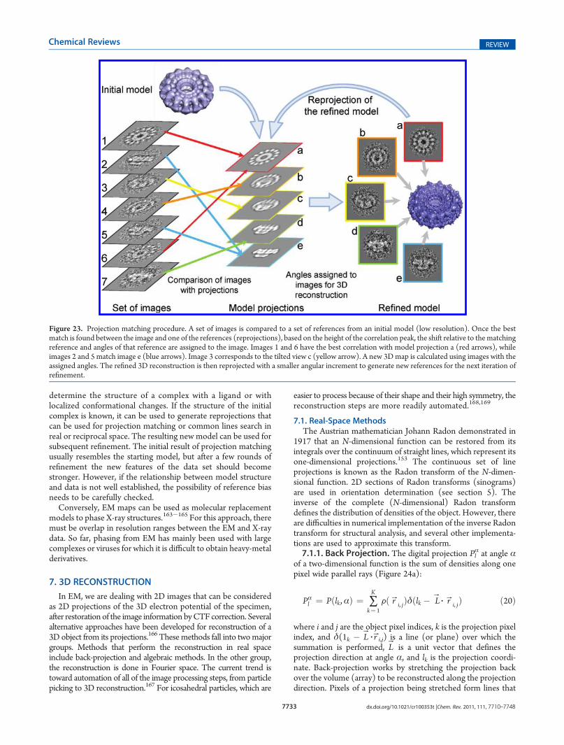
7733 dx.doi.org/10.1021/cr100353t |Chem. Rev. 2011, 111, 7710–7748
Chemical Reviews REVIEW
determine the structure of a complex with a ligand or withlocalized conformational changes. If the structure of the initialcomplex is known, it can be used to generate reprojections thatcan be used for projection matching or common lines search inreal or reciprocal space. The resulting new model can be used forsubsequent refinement. The initial result of projection matchingusually resembles the starting model, but after a few rounds ofrefinement the new features of the data set should becomestronger. However, if the relationship between model structureand data is not well established, the possibility of reference biasneeds to be carefully checked.
Conversely, EM maps can be used as molecular replacementmodels to phase X-ray structures.163�165 For this approach, theremust be overlap in resolution ranges between the EM and X-raydata. So far, phasing from EM has mainly been used with largecomplexes or viruses for which it is difficult to obtain heavy-metalderivatives.
7. 3D RECONSTRUCTION
In EM, we are dealing with 2D images that can be consideredas 2D projections of the 3D electron potential of the specimen,after restoration of the image information byCTF correction. Severalalternative approaches have been developed for reconstruction of a3D object from its projections.166 These methods fall into twomajorgroups. Methods that perform the reconstruction in real spaceinclude back-projection and algebraic methods. In the other group,the reconstruction is done in Fourier space. The current trend istoward automation of all of the image processing steps, from particlepicking to 3D reconstruction.167 For icosahedral particles, which are
easier to process because of their shape and their high symmetry, thereconstruction steps are more readily automated.168,169
7.1. Real-Space MethodsThe Austrian mathematician Johann Radon demonstrated in
1917 that an N-dimensional function can be restored from itsintegrals over the continuum of straight lines, which represent itsone-dimensional projections.153 The continuous set of lineprojections is known as the Radon transform of the N-dimen-sional function. 2D sections of Radon transforms (sinograms)are used in orientation determination (see section 5). Theinverse of the complete (N-dimensional) Radon transformdefines the distribution of densities of the object. However, thereare difficulties in numerical implementation of the inverse Radontransform for structural analysis, and several other implementa-tions are used to approximate this transform.7.1.1. Back Projection. The digital projection Pl
α at angle αof a two-dimensional function is the sum of densities along onepixel wide parallel rays (Figure 24a):
Pαl ¼ Pðlk,αÞ ¼ ∑K
k¼ 1Fð rBi, jÞδðlk � LB 3 rBi, jÞ ð20Þ
where i and j are the object pixel indices, k is the projection pixelindex, and δ(1k � LB 3 rBi,j) is a line (or plane) over which thesummation is performed, LB is a unit vector that defines theprojection direction at angle α, and lk is the projection coordi-nate. Back-projection works by stretching the projection backover the volume (array) to be reconstructed along the projectiondirection. Pixels of a projection being stretched form lines that
Figure 23. Projection matching procedure. A set of images is compared to a set of references from an initial model (low resolution). Once the bestmatch is found between the image and one of the references (reprojections), based on the height of the correlation peak, the shift relative to thematchingreference and angles of that reference are assigned to the image. Images 1 and 6 have the best correlation with model projection a (red arrows), whileimages 2 and 5 match image e (blue arrows). Image 3 corresponds to the tilted view c (yellow arrow). A new 3Dmap is calculated using images with theassigned angles. The refined 3D reconstruction is then reprojected with a smaller angular increment to generate new references for the next iteration ofrefinement.

7734 dx.doi.org/10.1021/cr100353t |Chem. Rev. 2011, 111, 7710–7748
Chemical Reviews REVIEW
are called ray sums (RS). An estimate of the density in a givenpixel of the reconstruction with coordinates i,j is the sum of allRSs that pass through that pixel (Figure 24b). However, thissimple technique does not accurately reconstruct the originalobject; details are smeared over some distance or surrounded bya halo (Figure 24C and D). These distortions arise because thereconstruction is convoluted with a broad PSF, which has a falloffof 1/r in 2D and 1/r2 in 3D space:
Frecð rBÞ ¼ Forigð rBÞ X1r
in 2D space ð21aÞ
Frecð rBÞ ¼ Forigð rBÞ X1r2
in 3D space ð21bÞ
or where X is the convolution operator and rB is the real spacevector.124,170
7.1.2. Filtered Back-Projection or Convolution Methods.Filtered back-projection is a modified version of the back-projection algorithm, which corrects for the blurring introducedby the PSF function mentioned in section 7.1.1 (Figure 25). Theoperation can be performed in either real or Fourier space. InFourier space, the correction is achieved by applying a filtercorresponding to the inverse of the PSF. For 1/r, this function isproportional to the spatial frequency and is called a ramp filter.A variety of filters can be used in real space. One type of filter
used for correcting back projection is the Laplace operator, whichis applied to the projections for prefiltering. These reconstructionalgorithms are based on functions that approximate the inverseRadon transform; they perform back-projection reconstructionon the preprocessed projections.171�173 The preprocessingmodifies the projections using window (apodizing) functions(Hamming window), which are equal to zero outside a chosendistance interval and enhance the signal within the interval.170 In
some packages, the filtering is performed in 3D space on thereconstruction obtained by back-projection.Filter characteristics in addition to the 1/r term depend on
the distribution of projections and their noise level, as well asthe symmetry of the object.149,174,175 Most published filterfunctions have been derived analytically from theoreticalconsiderations.170,173
7.1.3. Algebraic Methods. The development of algebraicmethods has been stimulated by medical tomography. In thiscase, reconstruction of the 3D object is based on determinationof successive planar slices of the object (patient), so that theproblem is reduced to a set of 2D reconstructions from 1Dprojections. We will explain the methods in 2D space, becausethe concept of reconstruction can be easily extended to 3D space.This technique requires that the object is described by a
positive function over a finite region (the object is of limitedsize) and can be represented as a digital I � J array of densities.An element of the array with coordinates i, j is the pixel Fi,j. Theprojection Pl
α is defined as in eq 20:
Pαl ¼ ∑l
i, j ∈ rayðl ,αÞFi, j ð22Þ
where i = 1, 2, ..., I; j = 1, 2, ..., J; l = 1, 2, ..., L.Equation 22 is linear, with I unknowns. For M projections,
there will be L�M linear equations. Solution of the complete setof equations would give the reconstruction of the object. Theproblem arises from the fact that a number of unknowns I � J(the size of the array {F(rBi,j)}) can be larger than number ofequations in the set (L 3M), and that the number of unknownsincreases dramatically with image dimensions. If L �M < I � J,the set of equations can have more than one solution. Moreover,in reality, projections may not be consistent with each otherbecause of noise. Even for an image of 50� 50 pixels, the number
Figure 24. Back-projection algorithm. (a) Projections Plα1, Pl
α2, and Plα3 are obtained experimentally from an object containing two dots of different
density. α1, α2, and α3 are the angles of the different projection directions, and Lα1, Lα2, and Lα3 are the unit vectors of the corresponding projectiondirections (eq 20). (b) Back projection is done by stretching projections back through the area to be reconstructed along the original projectiondirections, or in other words by creating rays of pixels with the density of the corresponding projection pixel. This is shown as light and dark gray linesfrom projections 1, 2, and 3. The rays are summed in the reconstructed area, providing information on the dot positions. (c) The more projections thatare used, the better defined are the dots. (d) An artifact of the technique is that each point is surrounded by a background halo. The intensity of the halo isproportional to the density of the dot.
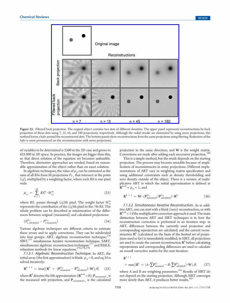
7735 dx.doi.org/10.1021/cr100353t |Chem. Rev. 2011, 111, 7710–7748
Chemical Reviews REVIEW
of variables to be determined is 2500 in the 2D case and grows to625 000 in 3D space. In practice, the images are bigger than this,so that direct solution of the equation set becomes unfeasible.Therefore, alternative approaches are needed, based on reason-able approximation of the object rather than on exact solution.In algebraic techniques, the value of Fi,j can be estimated as the
sum of all RSs from M projections Plαm that intersect at the point(i,j), multiplied by a weighting factor, where each RS is one pixelwide.
Fi, j ¼ ∑M
m¼ 1RSml 3W
mi, j ð23Þ
where RSl passes through (i,j)th pixel. The weight factor Wi,jm
represents the contribution of the (i,j)th pixel to the l th RS. Thewhole problem can be described as minimization of the differ-ences between original (measured) and calculated projections:
ðPαml, calculated � Pαm
l, measuredÞ ð24ÞVarious algebraic techniques use different criteria to estimatethese errors and to apply corrections. They can be subdividedinto four groups: ART, algebraic reconstruction technique;176
SIRT,177 simultaneous iterative reconstruction technique; SART,simultaneous algebraic reconstruction technique;177 and RMLE,relaxation methods for linear equations.170,178,179
7.1.3.1. Algebraic Reconstruction Technique. In ART, theinitial array (the first approximation) is blank: Fi,j = 0, and eq 24 issolved iteratively:
Rk þ 1 ¼ max½ðRk þ ðPαmmeasured � Pαm
calculatedÞ 3WÞ, 0� ð25ÞwhereRk denotes the kth approximation (Rk=0 = 0);Pmeasuredαm isthe measured mth projection, and Pcalculatedαm is the calculated
projection in the same direction; and W is the weight matrix.Corrections are made after adding each successive projection.180
This is a simple method, but the result depends on the startingprojection. The process may become unstable because of ampli-fication of inconsistencies in noisy projections. Different imple-mentations of ART vary in weighting matrix specification andusing additional constraints such as density thresholding andzero density outside of the object. There is a version of multi-plicative ART in which the initial approximation is defined asRk=0 = Fi,j = 1, and
Rk þ 1 ¼ W 3 ðPαmmeasured=P
αmcalculatedÞ 3Rk ð26Þ
7.1.3.2. Simultaneous Iterative Reconstruction. As in addi-tive ART, one can start with a blank (zero) reconstruction, or withRk=0 = 1 if themultiplicative correction approach is used. Themaindistinction between ART and SIRT techniques is in how thereconstruction correction is performed in an iteration step: inART, differences between the currently used projection andcorresponding reprojection are calculated, and the current recon-struction Rk (calculated on the basis of the limited set of projec-tions used so far) is immediately modified; in SIRT, all projectionsare used to create the current reconstruction Rk before calculatingreprojections and corresponding differences are used to calculatean overall corrective matrix for the next iteration:
Rk þ 1
¼ max½ðRk þ ðA 3∑Pαmmeasured � B 3∑Pαm
calculatedÞ 3WÞ, 0� ð27Þwhere A and B are weighting parameters.181 Results of SIRT donot depend on the starting projection. Although SIRT convergesmore slowly than ART, it produces better results.182
Figure 25. Filtered back projection. The original object contains two dots of different densities. The upper panel represents reconstructions by backprojection of these dots using 7, 15, 45, and 180 projections, respectively. Although the radial streaks are eliminated by using more projections, thismethod leaves a halo around the reconstructed dots. The bottom panels show reconstructions from the same projections using filtering. Reduction of thehalo is most pronounced on the reconstructions with more projections.
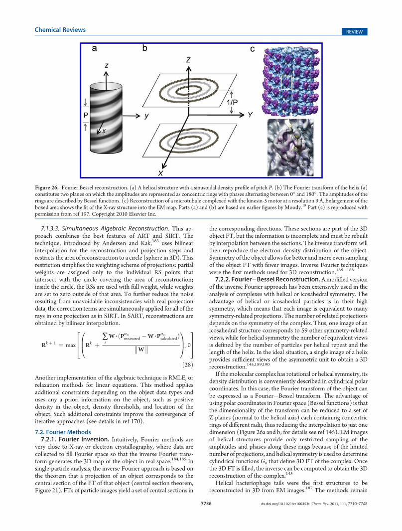
7736 dx.doi.org/10.1021/cr100353t |Chem. Rev. 2011, 111, 7710–7748
Chemical Reviews REVIEW
7.1.3.3. Simultaneous Algebraic Reconstruction. This ap-proach combines the best features of ART and SIRT. Thetechnique, introduced by Andersen and Kak,183 uses bilinearinterpolation for the reconstruction and projection steps andrestricts the area of reconstruction to a circle (sphere in 3D). Thisrestriction simplifies the weighting scheme of projections: partialweights are assigned only to the individual RS points thatintersect with the circle covering the area of reconstruction;inside the circle, the RSs are used with full weight, while weightsare set to zero outside of that area. To further reduce the noiseresulting from unavoidable inconsistencies with real projectiondata, the correction terms are simultaneously applied for all of therays in one projection as in SIRT. In SART, reconstructions areobtained by bilinear interpolation.
Rk þ 1 ¼ max Rk þ∑iW 3 ðPαm
measured �W 3PαmcalculatedÞ��W��
0B@
1CA, 0
264
375
ð28ÞAnother implementation of the algebraic technique is RMLE, orrelaxation methods for linear equations. This method appliesadditional constraints depending on the object data types anduses any a priori information on the object, such as positivedensity in the object, density thresholds, and location of theobject. Such additional constraints improve the convergence ofiterative approaches (see details in ref 170).
7.2. Fourier Methods7.2.1. Fourier Inversion. Intuitively, Fourier methods are
very close to X-ray or electron crystallography, where data arecollected to fill Fourier space so that the inverse Fourier trans-form generates the 3D map of the object in real space.184,185 Insingle-particle analysis, the inverse Fourier approach is based onthe theorem that a projection of an object corresponds to thecentral section of the FT of that object (central section theorem,Figure 21). FTs of particle images yield a set of central sections in
the corresponding directions. These sections are part of the 3Dobject FT, but the information is incomplete and must be rebuiltby interpolation between the sections. The inverse transform willthen reproduce the electron density distribution of the object.Symmetry of the object allows for better andmore even samplingof the object FT with fewer images. Inverse Fourier techniqueswere the first methods used for 3D reconstruction.186�188
7.2.2. Fourier�Bessel Reconstruction.Amodified versionof the inverse Fourier approach has been extensively used in theanalysis of complexes with helical or icosahedral symmetry. Theadvantage of helical or icosahedral particles is in their highsymmetry, which means that each image is equivalent to manysymmetry-related projections. The number of related projectionsdepends on the symmetry of the complex. Thus, one image of anicosahedral structure corresponds to 59 other symmetry-relatedviews, while for helical symmetry the number of equivalent viewsis defined by the number of particles per helical repeat and thelength of the helix. In the ideal situation, a single image of a helixprovides sufficient views of the asymmetric unit to obtain a 3Dreconstruction.145,189,190
If themolecular complex has rotational or helical symmetry, itsdensity distribution is conveniently described in cylindrical polarcoordinates. In this case, the Fourier transform of the object canbe expressed as a Fourier�Bessel transform. The advantage ofusing polar coordinates in Fourier space (Bessel functions) is thatthe dimensionality of the transform can be reduced to a set ofZ-planes (normal to the helical axis) each containing concentricrings of different radii, thus reducing the interpolation to just onedimension (Figure 26a and b; for details see ref 145). EM imagesof helical structures provide only restricted sampling of theamplitudes and phases along these rings because of the limitednumber of projections, and helical symmetry is used to determinecylindrical functions Gn that define 3D FT of the complex. Oncethe 3D FT is filled, the inverse can be computed to obtain the 3Dreconstruction of the complex.145
Helical bacteriophage tails were the first structures to bereconstructed in 3D from EM images.187 The methods remain
Figure 26. Fourier Bessel reconstruction. (a) A helical structure with a sinusoidal density profile of pitch P. (b) The Fourier transform of the helix (a)constitutes two planes on which the amplitudes are represented as concentric rings with phases alternating between 0� and 180�. The amplitudes of therings are described by Bessel functions. (c) Reconstruction of a microtubule complexed with the kinesin-5 motor at a resolution 9 Å. Enlargement of theboxed area shows the fit of the X-ray structure into the EM map. Parts (a) and (b) are based on earlier figures by Moody.19 Part (c) is reproduced withpermission from ref 197. Copyright 2010 Elsevier Inc.
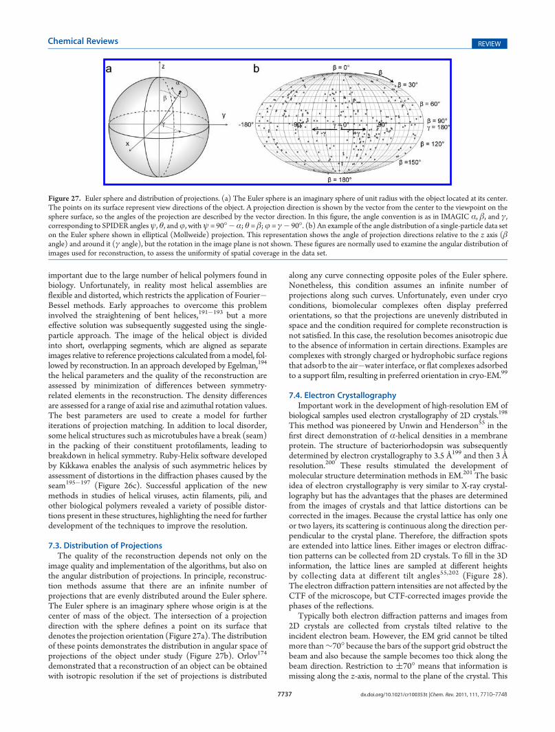
7737 dx.doi.org/10.1021/cr100353t |Chem. Rev. 2011, 111, 7710–7748
Chemical Reviews REVIEW
important due to the large number of helical polymers found inbiology. Unfortunately, in reality most helical assemblies areflexible and distorted, which restricts the application of Fourier�Bessel methods. Early approaches to overcome this probleminvolved the straightening of bent helices,191�193 but a moreeffective solution was subsequently suggested using the single-particle approach. The image of the helical object is dividedinto short, overlapping segments, which are aligned as separateimages relative to reference projections calculated from amodel, fol-lowed by reconstruction. In an approach developed by Egelman,194
the helical parameters and the quality of the reconstruction areassessed by minimization of differences between symmetry-related elements in the reconstruction. The density differencesare assessed for a range of axial rise and azimuthal rotation values.The best parameters are used to create a model for furtheriterations of projection matching. In addition to local disorder,some helical structures such as microtubules have a break (seam)in the packing of their constituent protofilaments, leading tobreakdown in helical symmetry. Ruby-Helix software developedby Kikkawa enables the analysis of such asymmetric helices byassessment of distortions in the diffraction phases caused by theseam195�197 (Figure 26c). Successful application of the newmethods in studies of helical viruses, actin filaments, pili, andother biological polymers revealed a variety of possible distor-tions present in these structures, highlighting the need for furtherdevelopment of the techniques to improve the resolution.
7.3. Distribution of ProjectionsThe quality of the reconstruction depends not only on the
image quality and implementation of the algorithms, but also onthe angular distribution of projections. In principle, reconstruc-tion methods assume that there are an infinite number ofprojections that are evenly distributed around the Euler sphere.The Euler sphere is an imaginary sphere whose origin is at thecenter of mass of the object. The intersection of a projectiondirection with the sphere defines a point on its surface thatdenotes the projection orientation (Figure 27a). The distributionof these points demonstrates the distribution in angular space ofprojections of the object under study (Figure 27b). Orlov174
demonstrated that a reconstruction of an object can be obtainedwith isotropic resolution if the set of projections is distributed
along any curve connecting opposite poles of the Euler sphere.Nonetheless, this condition assumes an infinite number ofprojections along such curves. Unfortunately, even under cryoconditions, biomolecular complexes often display preferredorientations, so that the projections are unevenly distributed inspace and the condition required for complete reconstruction isnot satisfied. In this case, the resolution becomes anisotropic dueto the absence of information in certain directions. Examples arecomplexes with strongly charged or hydrophobic surface regionsthat adsorb to the air�water interface, or flat complexes adsorbedto a support film, resulting in preferred orientation in cryo-EM.99
7.4. Electron CrystallographyImportant work in the development of high-resolution EM of
biological samples used electron crystallography of 2D crystals.198
This method was pioneered by Unwin and Henderson55 in thefirst direct demonstration of α-helical densities in a membraneprotein. The structure of bacteriorhodopsin was subsequentlydetermined by electron crystallography to 3.5 Å199 and then 3 Åresolution.200 These results stimulated the development ofmolecular structure determination methods in EM.201 The basicidea of electron crystallography is very similar to X-ray crystal-lography but has the advantages that the phases are determinedfrom the images of crystals and that lattice distortions can becorrected in the images. Because the crystal lattice has only oneor two layers, its scattering is continuous along the direction per-pendicular to the crystal plane. Therefore, the diffraction spotsare extended into lattice lines. Either images or electron diffrac-tion patterns can be collected from 2D crystals. To fill in the 3Dinformation, the lattice lines are sampled at different heightsby collecting data at different tilt angles55,202 (Figure 28).The electron diffraction pattern intensities are not affected by theCTF of the microscope, but CTF-corrected images provide thephases of the reflections.
Typically both electron diffraction patterns and images from2D crystals are collected from crystals tilted relative to theincident electron beam. However, the EM grid cannot be tiltedmore than∼70� because the bars of the support grid obstruct thebeam and also because the sample becomes too thick along thebeam direction. Restriction to (70� means that information ismissing along the z-axis, normal to the plane of the crystal. This
Figure 27. Euler sphere and distribution of projections. (a) The Euler sphere is an imaginary sphere of unit radius with the object located at its center.The points on its surface represent view directions of the object. A projection direction is shown by the vector from the center to the viewpoint on thesphere surface, so the angles of the projection are described by the vector direction. In this figure, the angle convention is as in IMAGIC α, β, and γ,corresponding to SPIDER anglesψ, θ, andj, withψ = 90��α; θ = β;j = γ� 90�. (b) An example of the angle distribution of a single-particle data seton the Euler sphere shown in elliptical (Mollweide) projection. This representation shows the angle of projection directions relative to the z axis (βangle) and around it (γ angle), but the rotation in the image plane is not shown. These figures are normally used to examine the angular distribution ofimages used for reconstruction, to assess the uniformity of spatial coverage in the data set.
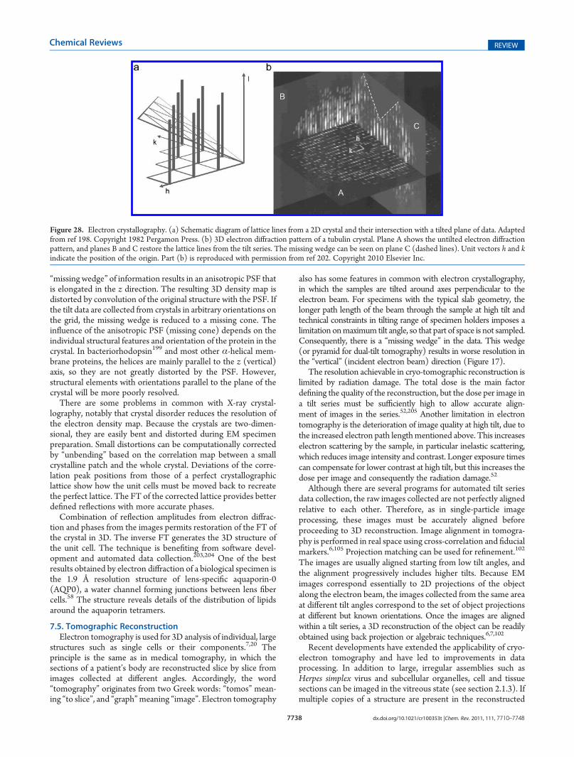
7738 dx.doi.org/10.1021/cr100353t |Chem. Rev. 2011, 111, 7710–7748
Chemical Reviews REVIEW
“missing wedge” of information results in an anisotropic PSF thatis elongated in the z direction. The resulting 3D density map isdistorted by convolution of the original structure with the PSF. Ifthe tilt data are collected from crystals in arbitrary orientations onthe grid, the missing wedge is reduced to a missing cone. Theinfluence of the anisotropic PSF (missing cone) depends on theindividual structural features and orientation of the protein in thecrystal. In bacteriorhodopsin199 and most other α-helical mem-brane proteins, the helices are mainly parallel to the z (vertical)axis, so they are not greatly distorted by the PSF. However,structural elements with orientations parallel to the plane of thecrystal will be more poorly resolved.
There are some problems in common with X-ray crystal-lography, notably that crystal disorder reduces the resolution ofthe electron density map. Because the crystals are two-dimen-sional, they are easily bent and distorted during EM specimenpreparation. Small distortions can be computationally correctedby “unbending” based on the correlation map between a smallcrystalline patch and the whole crystal. Deviations of the corre-lation peak positions from those of a perfect crystallographiclattice show how the unit cells must be moved back to recreatethe perfect lattice. The FT of the corrected lattice provides betterdefined reflections with more accurate phases.
Combination of reflection amplitudes from electron diffrac-tion and phases from the images permits restoration of the FT ofthe crystal in 3D. The inverse FT generates the 3D structure ofthe unit cell. The technique is benefiting from software devel-opment and automated data collection.203,204 One of the bestresults obtained by electron diffraction of a biological specimen isthe 1.9 Å resolution structure of lens-specific aquaporin-0(AQP0), a water channel forming junctions between lens fibercells.58 The structure reveals details of the distribution of lipidsaround the aquaporin tetramers.
7.5. Tomographic ReconstructionElectron tomography is used for 3D analysis of individual, large
structures such as single cells or their components.7,20 Theprinciple is the same as in medical tomography, in which thesections of a patient’s body are reconstructed slice by slice fromimages collected at different angles. Accordingly, the word“tomography” originates from two Greek words: “tomos” mean-ing “to slice”, and “graph”meaning “image”. Electron tomography
also has some features in common with electron crystallography,in which the samples are tilted around axes perpendicular to theelectron beam. For specimens with the typical slab geometry, thelonger path length of the beam through the sample at high tilt andtechnical constraints in tilting range of specimen holders imposes alimitation onmaximum tilt angle, so that part of space is not sampled.Consequently, there is a “missing wedge” in the data. This wedge(or pyramid for dual-tilt tomography) results in worse resolution inthe “vertical” (incident electron beam) direction (Figure 17).
The resolution achievable in cryo-tomographic reconstruction islimited by radiation damage. The total dose is the main factordefining the quality of the reconstruction, but the dose per image ina tilt series must be sufficiently high to allow accurate align-ment of images in the series.52,205 Another limitation in electrontomography is the deterioration of image quality at high tilt, due tothe increased electron path lengthmentioned above. This increaseselectron scattering by the sample, in particular inelastic scattering,which reduces image intensity and contrast. Longer exposure timescan compensate for lower contrast at high tilt, but this increases thedose per image and consequently the radiation damage.52
Although there are several programs for automated tilt seriesdata collection, the raw images collected are not perfectly alignedrelative to each other. Therefore, as in single-particle imageprocessing, these images must be accurately aligned beforeproceeding to 3D reconstruction. Image alignment in tomogra-phy is performed in real space using cross-correlation and fiducialmarkers.6,105 Projection matching can be used for refinement.102
The images are usually aligned starting from low tilt angles, andthe alignment progressively includes higher tilts. Because EMimages correspond essentially to 2D projections of the objectalong the electron beam, the images collected from the same areaat different tilt angles correspond to the set of object projectionsat different but known orientations. Once the images are alignedwithin a tilt series, a 3D reconstruction of the object can be readilyobtained using back projection or algebraic techniques.6,7,102
Recent developments have extended the applicability of cryo-electron tomography and have led to improvements in dataprocessing. In addition to large, irregular assemblies such asHerpes simplex virus and subcellular organelles, cell and tissuesections can be imaged in the vitreous state (see section 2.1.3). Ifmultiple copies of a structure are present in the reconstructed
Figure 28. Electron crystallography. (a) Schematic diagram of lattice lines from a 2D crystal and their intersection with a tilted plane of data. Adaptedfrom ref 198. Copyright 1982 Pergamon Press. (b) 3D electron diffraction pattern of a tubulin crystal. Plane A shows the untilted electron diffractionpattern, and planes B and C restore the lattice lines from the tilt series. The missing wedge can be seen on plane C (dashed lines). Unit vectors h and kindicate the position of the origin. Part (b) is reproduced with permission from ref 202. Copyright 2010 Elsevier Inc.
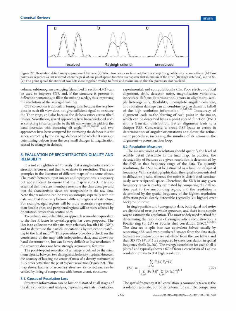
7739 dx.doi.org/10.1021/cr100353t |Chem. Rev. 2011, 111, 7710–7748
Chemical Reviews REVIEW
volume, subtomogram averaging (described in section 4.4.2) canbe used to improve SNR and, if the structure is present indifferent orientations, to fill in the missing wedge, thus improvingthe resolution of the averaged volumes.
CTF correction is difficult in tomograms, because the very lowdose in each tilt view does not give sufficient signal to measurethe Thon rings, and also because the defocus varies across tiltedimages. Nevertheless, several approaches have been developed, suchas correcting in bands parallel to the tilt axis, where the width of theband decreases with increasing tilt angle,102,151,206,207 and twoapproaches have been compared for estimating the defocus in a tiltseries: correcting by the average defocus of the whole tilt series, ordetermining defocus from the very small changes in magnificationcaused by changes in defocus.
8. EVALUATION OF RECONSTRUCTION QUALITY ANDRELIABILITY
It is not straightforward to verify that a single-particle recon-struction is correct and then to evaluate its resolution. There areexamples in the literature of different maps of the same object.The match between input images and reprojections is necessarybut not sufficient to ensure that the map is correct. It is alsoessential that the class members resemble the class averages andthat the characteristic views are recognizable in the raw data.Note that resolution can be very anisotropic, especially with tiltdata, and that it can vary between different regions of a structure.For example, rigid regions will be more accurately representedthan flexible ones, and peripheral regions will be more affected byorientation errors than central ones.
To evaluate map reliability, an approach somewhat equivalentto the free R factor in crystallography has been proposed. Theidea is to collect some tilt pairs, with relatively low tilt (10�30�),and to determine the particle orientations by projection match-ing to the final map.208 This procedure provides a check on theconsistency of the map with independent data, and allows forhand determination, but can be very difficult at low resolution ifthe structure does not have strongly asymmetric features.
The point-to-point resolution of an image is defined by the mini-mumdistance between two distinguishable densitymaxima.However,the accuracy of locating the center of mass of a density maximum is3�5 times better than the point to point resolution (Figure 29). If themap shows features of secondary structure, its correctness can beverified by fitting of components with known atomic structures.
8.1. Causes of Resolution LossStructure information can be lost or distorted at all stages of
the data collection and analysis, depending on instrumentation,
experimental, and computational skills. Poor electron opticalalignment, drift, detector noise, magnification variations,inaccurate defocus determination, errors in alignment, sam-ple heterogeneity, flexibility, incomplete angular coverage,and radiation damage can all combine to give dramatic falloffof the high-resolution information.10,208,209 Inaccuracy ofalignment leads to the blurring of each point in the image,which can be described by as a point spread function (PSF)with a Gaussian distribution. Better alignment leads to asharper PSF. Conversely, a broad PSF leads to errors indetermination of angular orientations and slows the refine-ment procedure, increasing the number of iterations in thealignment�reconstruction loop.
8.2. Resolution MeasuresThe measurement of resolution should quantify the level of
reliable detail detectable in the final map. In practice, thedetectability of features at a given resolution is determined bythe SNR in that frequency range of the data. To quantifyresolution, the SNR must be estimated as a function of spatialfrequency.With crystallographic data, the signal is concentratedin diffraction peaks, whereas the noise is distributed continu-ously over reciprocal space. Therefore, the SNR in any givenfrequency range is readily estimated by comparing the diffrac-tion peak to the surrounding region, and the resolution isdetermined by the spatial frequency of the highest resolutiondiffraction peaks clearly detectable (typically 3� higher) overbackground noise.
In single-particle and tomography data, both signal and noiseare distributed over the whole spectrum, and there is no simpleway to estimate the resolution. The most widely used method fordetermining the resolution of a single-particle reconstruction isFourier ring (in 2D) or Fourier shell correlation (FSC).210,211
The data set is split into two equivalent halves, usually byseparating odd- and even-numbered images from the data stack.Separate reconstructions are calculated from the two halves, andtheir 3D FTs (F1, F2) are compared by cross-correlation in spatialfrequency shells (k,Δk). The average correlation for each shell isplotted and typically shows a falloff from a correlation of 1 at lowresolution down to 0 at high resolution.
FSC ¼∑k,Δk
F1ðkÞF2�ðkÞ
j ∑k,Δk
jF1ðkÞj2 ∑k,Δk
jF2ðkÞj2j1=2ð29Þ
The spatial frequency at 0.5 correlation is commonly taken as theresolution estimate, but other criteria, for example, comparison
Figure 29. Resolution definition by separation of features. (a) When two points are far apart, there is a deep trough of density between them. (b) Twopoints are regarded as just resolved when the peak of one point spread function overlaps the first minimum of the other (Rayleigh criterion), see ref 60.(c) The point spread functions of two dots close together overlap to form one maximum, so that the points are not resolved.
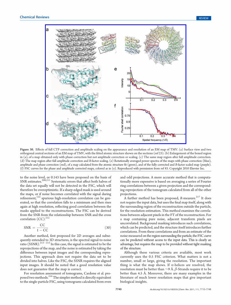
7740 dx.doi.org/10.1021/cr100353t |Chem. Rev. 2011, 111, 7710–7748
Chemical Reviews REVIEW
to the noise level, or 0.143 have been proposed on the basis ofSNR estimates.208,211 Systematic errors that affect both halves ofthe data set equally will not be detected in the FSC, which willtherefore be overoptimistic. If a sharp-edged mask is used aroundthe maps, or if noise becomes correlated with the signal duringrefinement,122 spurious high-resolution correlation can be gen-erated, so that the correlation falls to a minimum and then risesagain at high resolution, reflecting good correlation between themasks applied to the reconstructions. The FSC can be derivedfrom the SNR from the relationship between SNR and the crosscorrelation (CC).212
SNR ¼ CC1� CC
ð30ÞAnother method, first proposed for 2D averages and subse-
quently extended to 3D structures, is the spectral signal-to-noiseratio (SSNR).213�215 In this case, the signal is estimated to be thereprojections of the map, and the noise is estimated by taking thedifference between input images and the corresponding repro-jections. This approach does not require the data set to bedivided into halves. Like the FSC, the SSNR requires the alignedinput images. It should be noted that a good resolution valuedoes not guarantee that the map is correct.
For resolution assessment of tomograms, Cardone et al. pro-posed twomethods.216 The simpler method is directly equivalentto the single-particle FSC, using tomograms calculated from even
and odd projections. A more accurate method that is computa-tionally more expensive is based on averaging a series of Fourierring correlations between a given projection and the correspond-ing reprojection of the tomogram calculated from all of the otherprojections.
A further method has been proposed, R-measure.217 It doesnot require the input data, but uses the final map itself, along withthe surrounding region of the reconstruction outside the particle,for the resolution estimation. This method examines the correla-tions between adjacent pixels in the FT of the reconstruction. Fora map containing pure noise, adjacent transform pixels areuncorrelated. Background masking introduces such correlations,which can be predicted, and the structure itself introduces furthercorrelations. From these correlations and from an estimate of thenoisemeasured on the region surrounding theparticle, theFSCcurvecan be predicted without access to the input data. This is clearly anadvantage, but requires the map to be provided without tight maskingof the structure.
Although these various criteria are available, most workcurrently uses the 0.5 FSC criterion. What matters is not anumber, small or large, giving the resolution. The importantthing is what the map shows. If α-helices are resolved, theresolution must be better than∼9 Å. β-Strands require it to bebetter than 4.5 Å. Moreover, there are many examples in theliterature of much lower resolution maps that give importantbiological insights.
Figure 30. Effects of full CTF correction and amplitude scaling on the appearance and resolution of an EM map of TMV. (a) Surface view and twoorthogonal central sections of an EMmap of TMV, with the fitted atomic structure shown on the sections (ref 23). (b) Enlargement of the boxed regionin (a), of a map obtained only with phase correction but not amplitude correction or scaling. (c) The same map region after full amplitude correction.(d) The map region after full amplitude correction and B-factor scaling. (e) Rotationally averaged power spectra of the maps with phase correction (blue),amplitude and phase correction (red), of a map calculated from the atomic structure fit (green), and of the fully corrected and B-factor scaled map (purple).(f) FSC curves for the phase and amplitude corrected maps, colored as in (e). Reproduced with permission from ref 83. Copyright 2010 Elsevier Inc.
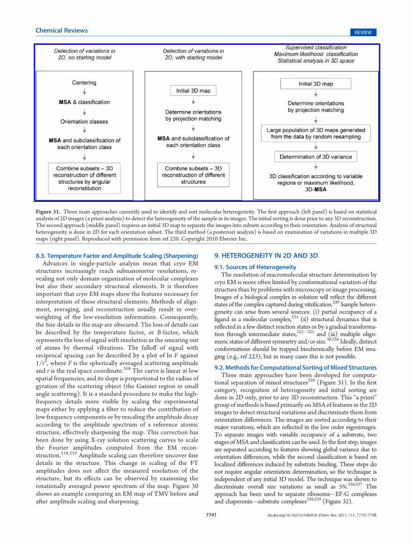
7741 dx.doi.org/10.1021/cr100353t |Chem. Rev. 2011, 111, 7710–7748
Chemical Reviews REVIEW
8.3. Temperature Factor and Amplitude Scaling (Sharpening)Advances in single-particle analysis mean that cryo EM
structures increasingly reach subnanometer resolutions, re-vealing not only domain organization of molecular complexesbut also their secondary structural elements. It is thereforeimportant that cryo EM maps show the features necessary forinterpretation of these structural elements. Methods of align-ment, averaging, and reconstruction usually result in over-weighting of the low-resolution information. Consequently,the fine details in the map are obscured. The loss of details canbe described by the temperature factor, or B-factor, whichrepresents the loss of signal with resolution as the smearing outof atoms by thermal vibrations. The falloff of signal withreciprocal spacing can be described by a plot of ln F against1/r2, where F is the spherically averaged scattering amplitudeand r is the real space coordinate.208 The curve is linear at lowspatial frequencies, and its slope is proportional to the radius ofgyration of the scattering object (the Guinier region in smallangle scattering). It is a standard procedure to make the high-frequency details more visible by scaling the experimentalmaps either by applying a filter to reduce the contribution oflow frequency components or by rescaling the amplitude decayaccording to the amplitude spectrum of a reference atomicstructure, effectively sharpening the map. This correction hasbeen done by using X-ray solution scattering curves to scalethe Fourier amplitudes computed from the EM recon-struction.218,219 Amplitude scaling can therefore uncover finedetails in the structure. This change in scaling of the FTamplitudes does not affect the measured resolution of thestructure, but its effects can be observed by examining therotationally averaged power spectrum of the map. Figure 30shows an example comparing an EM map of TMV before andafter amplitude scaling and sharpening.
9. HETEROGENEITY IN 2D AND 3D
9.1. Sources of HeterogeneityThe resolution of macromolecular structure determination by
cryo EM is more often limited by conformational variation of thestructure than by problems withmicroscopy or image processing.Images of a biological complex in solution will reflect the differentstates of the complex captured during vitrification.220 Sample hetero-geneity can arise from several sources: (i) partial occupancy of aligand in a molecular complex,221 (ii) structural dynamics that isreflected in a few distinct reaction states or by a gradual transforma-tion through intermediate states,222�225 and (iii) multiple oligo-meric states of different symmetry and/or size.30,226 Ideally, distinctconformations should be trapped biochemically before EM ima-ging (e.g., ref 223), but in many cases this is not possible.
9.2.Methods for Computational Sorting ofMixed StructuresThree main approaches have been developed for computa-
tional separation of mixed structures220 (Figure 31). In the firstcategory, recognition of heterogeneity and initial sorting aredone in 2D only, prior to any 3D reconstruction. This “a priori”group ofmethods is based primarily onMSA of features in the 2Dimages to detect structural variations and discriminate them fromorientation differences. The images are sorted according to theirmajor variations, which are reflected in the low order eigenimages.To separate images with variable occupancy of a substrate, twostages ofMSA and classification can be used. In the first step, imagesare separated according to features showing global variance due toorientation differences, while the second classification is based onlocalized differences induced by substrate binding. These steps donot require angular orientation determination, so the technique isindependent of any initial 3D model. The technique was shown todiscriminate overall size variations as small as 5%.226,227 Thisapproach has been used to separate ribosome�EF-G complexesand chaperonin�substrate complexes228,229 (Figure 32).
Figure 31. Three main approaches currently used to identify and sort molecular heterogeneity. The first approach (left panel) is based on statisticalanalysis of 2D images (a priori analysis) to detect the heterogeneity of the sample in its images. The initial sorting is done prior to any 3D reconstruction.The second approach (middle panel) requires an initial 3D map to separate the images into subsets according to their orientation. Analysis of structuralheterogeneity is done in 2D for each orientation subset. The third method (a posteriori analysis) is based on examination of variations in multiple 3Dmaps (right panel). Reproduced with permission from ref 220. Copyright 2010 Elsevier Inc.
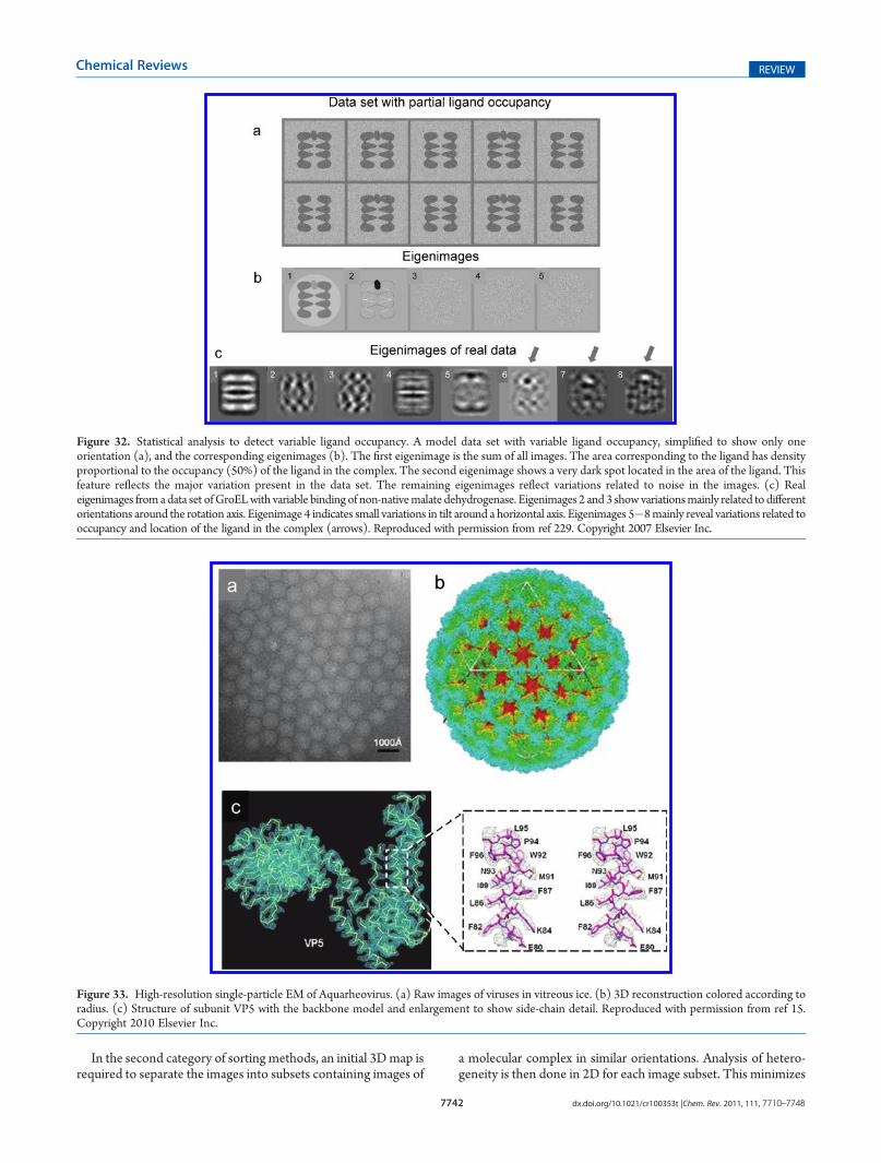
7742 dx.doi.org/10.1021/cr100353t |Chem. Rev. 2011, 111, 7710–7748
Chemical Reviews REVIEW
In the second category of sorting methods, an initial 3Dmap isrequired to separate the images into subsets containing images of
a molecular complex in similar orientations. Analysis of hetero-geneity is then done in 2D for each image subset. This minimizes
Figure 32. Statistical analysis to detect variable ligand occupancy. A model data set with variable ligand occupancy, simplified to show only oneorientation (a), and the corresponding eigenimages (b). The first eigenimage is the sum of all images. The area corresponding to the ligand has densityproportional to the occupancy (50%) of the ligand in the complex. The second eigenimage shows a very dark spot located in the area of the ligand. Thisfeature reflects the major variation present in the data set. The remaining eigenimages reflect variations related to noise in the images. (c) Realeigenimages fromadata set ofGroELwith variable binding of non-nativemalate dehydrogenase. Eigenimages 2 and 3 showvariationsmainly related to differentorientations around the rotation axis. Eigenimage 4 indicates small variations in tilt around a horizontal axis. Eigenimages 5�8mainly reveal variations related tooccupancy and location of the ligand in the complex (arrows). Reproduced with permission from ref 229. Copyright 2007 Elsevier Inc.
Figure 33. High-resolution single-particle EM of Aquarheovirus. (a) Raw images of viruses in vitreous ice. (b) 3D reconstruction colored according toradius. (c) Structure of subunit VP5 with the backbone model and enlargement to show side-chain detail. Reproduced with permission from ref 15.Copyright 2010 Elsevier Inc.
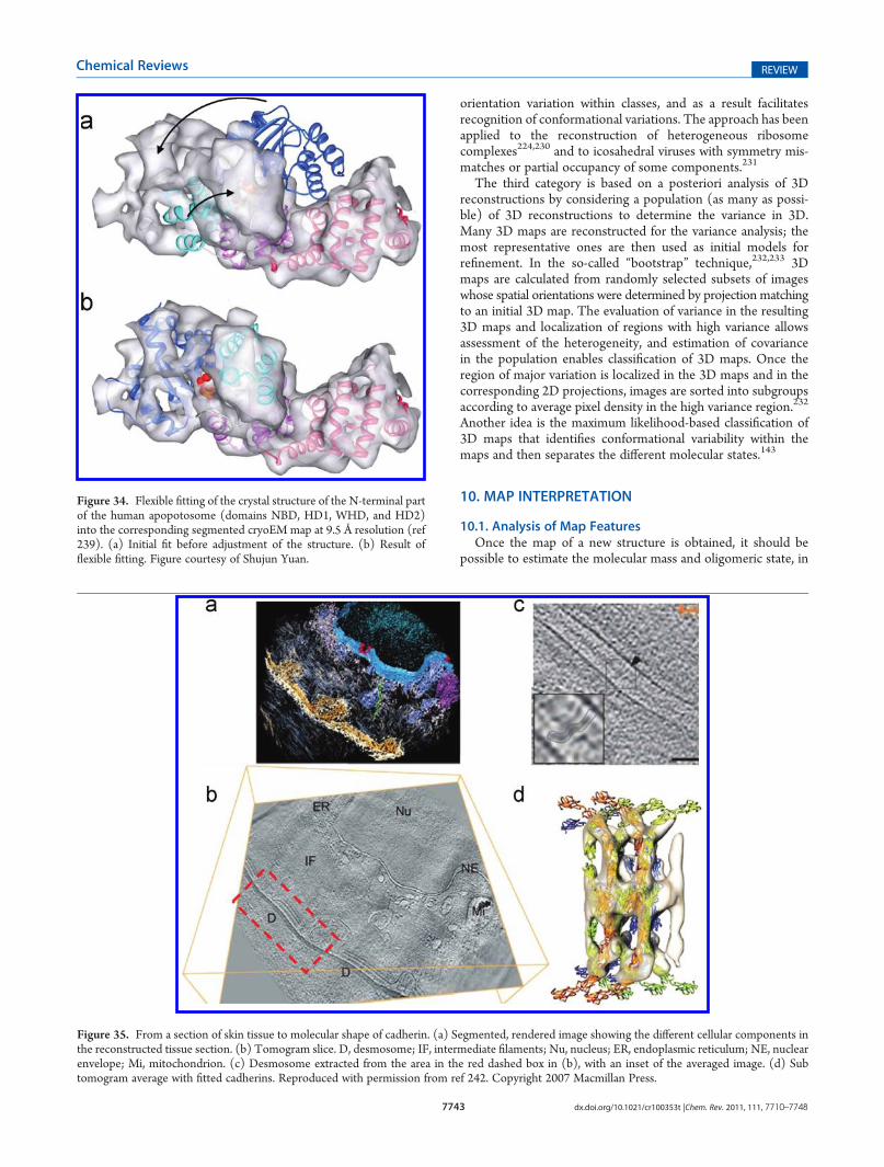
7743 dx.doi.org/10.1021/cr100353t |Chem. Rev. 2011, 111, 7710–7748
Chemical Reviews REVIEW
orientation variation within classes, and as a result facilitatesrecognition of conformational variations. The approach has beenapplied to the reconstruction of heterogeneous ribosomecomplexes224,230 and to icosahedral viruses with symmetry mis-matches or partial occupancy of some components.231
The third category is based on a posteriori analysis of 3Dreconstructions by considering a population (as many as possi-ble) of 3D reconstructions to determine the variance in 3D.Many 3D maps are reconstructed for the variance analysis; themost representative ones are then used as initial models forrefinement. In the so-called “bootstrap” technique,232,233 3Dmaps are calculated from randomly selected subsets of imageswhose spatial orientations were determined by projection matchingto an initial 3D map. The evaluation of variance in the resulting3D maps and localization of regions with high variance allowsassessment of the heterogeneity, and estimation of covariancein the population enables classification of 3D maps. Once theregion of major variation is localized in the 3D maps and in thecorresponding 2D projections, images are sorted into subgroupsaccording to average pixel density in the high variance region.232
Another idea is the maximum likelihood-based classification of3D maps that identifies conformational variability within themaps and then separates the different molecular states.143
10. MAP INTERPRETATION
10.1. Analysis of Map FeaturesOnce the map of a new structure is obtained, it should be
possible to estimate the molecular mass and oligomeric state, in
Figure 34. Flexible fitting of the crystal structure of the N-terminal partof the human apopotosome (domains NBD, HD1, WHD, and HD2)into the corresponding segmented cryoEM map at 9.5 Å resolution (ref239). (a) Initial fit before adjustment of the structure. (b) Result offlexible fitting. Figure courtesy of Shujun Yuan.
Figure 35. From a section of skin tissue to molecular shape of cadherin. (a) Segmented, rendered image showing the different cellular components inthe reconstructed tissue section. (b) Tomogram slice. D, desmosome; IF, intermediate filaments; Nu, nucleus; ER, endoplasmic reticulum; NE, nuclearenvelope; Mi, mitochondrion. (c) Desmosome extracted from the area in the red dashed box in (b), with an inset of the averaged image. (d) Subtomogram average with fitted cadherins. Reproduced with permission from ref 242. Copyright 2007 Macmillan Press.
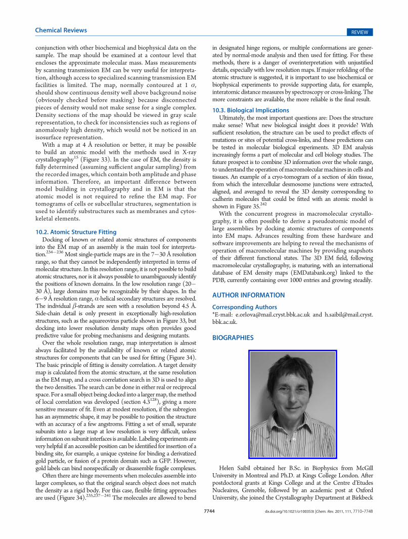
7744 dx.doi.org/10.1021/cr100353t |Chem. Rev. 2011, 111, 7710–7748
Chemical Reviews REVIEW
conjunction with other biochemical and biophysical data on thesample. The map should be examined at a contour level thatencloses the approximate molecular mass. Mass measurementsby scanning transmission EM can be very useful for interpreta-tion, although access to specialized scanning transmission EMfacilities is limited. The map, normally contoured at 1 σ,should show continuous density well above background noise(obviously checked before masking) because disconnectedpieces of density would not make sense for a single complex.Density sections of the map should be viewed in gray scalerepresentation, to check for inconsistencies such as regions ofanomalously high density, which would not be noticed in anisosurface representation.
With a map at 4 Å resolution or better, it may be possibleto build an atomic model with the methods used in X-raycrystallography15 (Figure 33). In the case of EM, the density isfully determined (assuming sufficient angular sampling) fromthe recorded images, which contain both amplitude and phaseinformation. Therefore, an important difference betweenmodel building in crystallography and in EM is that theatomic model is not required to refine the EM map. Fortomograms of cells or subcellular structures, segmentation isused to identify substructures such as membranes and cytos-keletal elements.
10.2. Atomic Structure FittingDocking of known or related atomic structures of components
into the EM map of an assembly is the main tool for interpreta-tion.234�236 Most single-particle maps are in the 7�30 Å resolutionrange, so that they cannot be independently interpreted in terms ofmolecular structure. In this resolution range, it is not possible to buildatomic structures, nor is it always possible to unambiguously identifythe positions of known domains. In the low resolution range (20�30 Å), large domains may be recognizable by their shapes. In the6�9 Å resolution range, α-helical secondary structures are resolved.The individual β-strands are seen with a resolution beyond 4.5 Å.Side-chain detail is only present in exceptionally high-resolutionstructures, such as the aquareovirus particle shown in Figure 33, butdocking into lower resolution density maps often provides goodpredictive value for probing mechanisms and designing mutants.
Over the whole resolution range, map interpretation is almostalways facilitated by the availability of known or related atomicstructures for components that can be used for fitting (Figure 34).The basic principle of fitting is density correlation. A target densitymap is calculated from the atomic structure, at the same resolutionas the EMmap, and a cross correlation search in 3D is used to alignthe two densities. The search can be done in either real or reciprocalspace. For a small object being docked into a largermap, themethodof local correlation was developed (section 4.3128), giving a moresensitive measure of fit. Even at modest resolution, if the subregionhas an asymmetric shape, it may be possible to position the structurewith an accuracy of a few angstroms. Fitting a set of small, separatesubunits into a large map at low resolution is very difficult, unlessinformationon subunit interfaces is available. Labeling experiments arevery helpful if an accessible position can be identified for insertion of abinding site, for example, a unique cysteine for binding a derivatizedgold particle, or fusion of a protein domain such as GFP. However,gold labels can bind nonspecifically or disassemble fragile complexes.
Often there are hinge movements whenmolecules assemble intolarger complexes, so that the original search object does not matchthe density as a rigid body. For this case, flexible fitting approachesare used (Figure 34).235,237�241 The molecules are allowed to bend
in designated hinge regions, or multiple conformations are gener-ated by normal-mode analysis and then used for fitting. For thesemethods, there is a danger of overinterpretation with unjustifieddetails, especially with low resolutionmaps. If major refolding of theatomic structure is suggested, it is important to use biochemical orbiophysical experiments to provide supporting data, for example,interatomic distancemeasures by spectroscopy or cross-linking. Themore constraints are available, the more reliable is the final result.
10.3. Biological ImplicationsUltimately, the most important questions are: Does the structure
make sense? What new biological insight does it provide? Withsufficient resolution, the structure can be used to predict effects ofmutations or sites of potential cross-links, and these predictions canbe tested in molecular biological experiments. 3D EM analysisincreasingly forms a part of molecular and cell biology studies. Thefuture prospect is to combine 3D information over the whole range,to understand the operationofmacromolecularmachines in cells andtissues. An example of a cryo-tomogram of a section of skin tissue,from which the intercellular desmosome junctions were extracted,aligned, and averaged to reveal the 3D density corresponding tocadherin molecules that could be fitted with an atomic model isshown in Figure 35.242
With the concurrent progress in macromolecular crystallo-graphy, it is often possible to derive a pseudoatomic model oflarge assemblies by docking atomic structures of componentsinto EM maps. Advances resulting from these hardware andsoftware improvements are helping to reveal the mechanisms ofoperation of macromolecular machines by providing snapshotsof their different functional states. The 3D EM field, followingmacromolecular crystallography, is maturing, with an internationaldatabase of EM density maps (EMDatabank.org) linked to thePDB, currently containing over 1000 entries and growing steadily.
AUTHOR INFORMATION
Corresponding Authors*E-mail: [email protected] and [email protected].
BIOGRAPHIES
Helen Saibil obtained her B.Sc. in Biophysics from McGillUniversity in Montreal and Ph.D. at Kings College London. Afterpostdoctoral grants at Kings College and at the Centre d’EtudesNucleaires, Grenoble, followed by an academic post at OxfordUniversity, she joined the Crystallography Department at Birkbeck
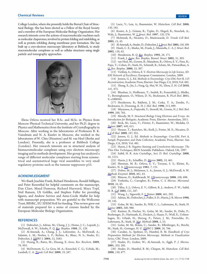
7745 dx.doi.org/10.1021/cr100353t |Chem. Rev. 2011, 111, 7710–7748
Chemical Reviews REVIEW
College London, where she presently holds the Bernal Chair of Struc-tural Biology. She has been elected as a Fellow of the Royal Societyand amember of the EuropeanMolecular BiologyOrganization. Herresearch interests cover the actions of macromolecular machines suchasmolecular chaperones, involved in protein folding andmisfolding, aswell as protein refolding during membrane pore formation. She hasbuilt up a cryo-electron microscopy laboratory at Birkbeck, to studymacromolecular complexes as well as cellular structures using singleparticle and tomography approaches.
Elena Orlova received her B.Sc. and M.Sc. in Physics fromMoscow Physical-Technical University, and her Ph.D. degree inPhysics andMathematics from the Institute of Crystallography inMoscow. After working in the laboratories of Professors B. K.Vainshtain and N. A. Kiselev in Moscow, she worked in thelaboratories of W. Chiu (Houston) and M. van Heel (Berlin andLondon). Presently, she is a professor at Birkbeck College(London). Her research interests are in structural analysis ofbiomacromolecular complexes using cryo electron microscopyimaging and in methods development. Her group has analyzed arange of different molecular complexes starting from symme-trical and asymmetrical huge viral assemblies to very smallregulatory proteins such as the tumour suppressor p53.
ACKNOWLEDGMENT
We thank Joachim Frank, Richard Henderson, Ronald Milligan,and Peter Rosenthal for helpful comments on the manuscript,Dan Clare, Maud Dumoux, Richard Hayward, Maya Topf,Neil Ranson, Uli Gohlke, and Stephen Fuller for providingfigures, and Andrew Service and Anne-Cecile Maffat for helpwith manuscript preparation. We are grateful to the WellcomeTrust, BBSRC, EU 3DEMNoE for funding. This review grew outof materials prepared for a series of courses funded by theEuropean Molecular Biology Organization.
REFERENCES
(1) Dubochet, J.; Adrian, M.; Chang, J. J.; Homo, J. C.; Lepault, J.;McDowall, A. W.; Schultz, P. Q. Rev. Biophys. 1988, 21, 129.(2) Al-Amoudi, A.; Chang, J. J.; Leforestier, A.; McDowall, A.;
Salamin, L. M.; Norlen, L. P.; Richter, K.; Blanc, N. S.; Studer, D.;Dubochet, J. EMBO J. 2004, 23, 3583.(3) Huang, B.; Bates, M.; Zhuang, X. Annu. Rev. Biochem. 2009,
78, 993.(4) McDermott, G.; Le Gros, M. A.; Knoechel, C. G.; Uchida, M.;
Larabell, C. A. Trends Cell Biol. 2009, 19, 587.
(5) Lucic, V.; Leis, A.; Baumeister, W. Histochem. Cell Biol. 2008,130, 185.
(6) Koster, A. J.; Grimm, R.; Typke, D.; Hegerl, R.; Stoschek, A.;Walz, J.; Baumeister, W. J. Struct. Biol. 1997, 120, 276.
(7) McIntosh, R.; Nicastro, D.; Mastronarde, D. Trends Cell Biol.2005, 15, 43.
(8) Al-Amoudi, A.; Studer,D.;Dubochet, J. J. Struct. Biol. 2005, 150, 109.(9) Hsieh, C. E.; Marko, M.; Frank, J.; Mannella, C. A. J. Struct. Biol.
2002, 138, 63.(10) Henderson, R. Q. Rev. Biophys. 1995, 28, 171.(11) Frank, J. Annu. Rev. Biophys. Biomol. Struct. 2002, 31, 303.(12) van Heel, M.; Gowen, B.; Matadeen, R.; Orlova, E. V.; Finn, R.;
Pape, T.; Cohen, D.; Stark, H.; Schmidt, R.; Schatz, M.; Patwardhan, A.Q. Rev. Biophys. 2000, 33, 307.
(13) Verkleij, A.; Orlova, E. V. Electron Microscopy in Life Science, 3D-EM Network of Excellence; European Commission: London, 2009.
(14) Jensen, G. J., Ed.Methods in Enzymology: Cryo-EM, Part B, 3-DReconstruction; Academic Press, Elsevier: San Diego, CA, 2010; Vol. 482.
(15) Zhang, X.; Jin, L.; Fang, Q.; Hui, W. H.; Zhou, Z. H. Cell 2010,141, 472.
(16) Bhushan, S.; Hoffmann, T.; Seidelt, B.; Frauenfeld, J.; Mielke,T.; Berninghausen, O.; Wilson, D. N.; Beckmann, R. PLoS Biol. 2011,9, e1000581.
(17) Henderson, R.; Baldwin, J. M.; Ceska, T. A.; Zemlin, F.;Beckmann, E.; Downing, K. H. J. Mol. Biol. 1990, 213, 899.
(18) Miyazawa, A.; Fujiyoshi, Y.; Stowell, M.; Unwin, N. J. Mol. Biol.1999, 288, 765.
(19) Moody, M. F. Structural Biology Using Electrons and X-rays. AnIntroduction for Biologists; Academic Press, Elsevier: Amsterdam, 2011.
(20) Beck, M.; Lucic, V.; F€orster, F.; Baumeister, W.; Medalia, O.Nature 2007, 449, 611.
(21) Heuser, T.; Raytchev, M.; Krell, J.; Porter, M. E.; Nicastro, D.J. Cell Biol. 2009, 187, 921.
(22) Jensen, G. J., Ed. Methods in Enzymology: Cryo-EM, Part A,Sample Preparation and Data Collection; Academic Press, Elsevier: SanDiego, CA, 2010; Vol. 481.
(23) Harris, J. R. Negative Staining and Cryoelectron Microscopy: TheThin Film Techniques; BIOS Scientific Publishers: Oxford, UK, 1997.
(24) Saibil, H. R. Acta Crystallogr., Sect. D: Biol. Crystallogr. 2000,56, 1215.
(25) Harris, J. R.; Scheffler, D. Micron 2002, 33, 461.(26) Sherman, M. B.; Orlova, E. V.; Terzyan, S. S.; Kleine, R.;
Kiselev, N. A. Ultramicroscopy 1981, 7, 131.(27) Dobro, M. J.; Melanson, L. A.; Jensen, G. J.; McDowall, A. W.
Methods Enzymol. 2010, 481, 63.(28) Rhinow, D.; Kuhlbrandt, W. Ultramicroscopy 2008, 108, 698.(29) Yoshioka, C.; Carragher, B.; Potter, C. S. Microsc. Microanal.
2010, 16, 43.(30) Tilley, S. J.; Orlova, E. V.; Gilbert, R. J.; Andrew, P. W.; Saibil,
H. R. Cell 2005, 121, 247.(31) Wang, L.; Sigworth, F. J. Nature 2009, 461, 292.(32) Adrian,M.; Dubochet, J.; Fuller, S. D.; Harris, J. R.Micron 1998,
29, 145.(33) Golas, M. M.; Sander, B.; Will, C. L.; Luhrmann, R.; Stark, H.
Science 2003, 300, 980.(34) Kastner, B.; Fischer, N.; Golas, M. M.; Sander, B.; Dube, P.;
Boehringer, D.; Hartmuth, K.; Deckert, J.; Hauer, F.; Wolf, E.; Uchten-hagen, H.; Urlaub, H.; Herzog, F.; Peters, J. M.; Poerschke, D.;Luhrmann, R.; Stark, H. Nat. Methods 2008, 5, 53.
(35) Golas, M. M.; Bohm, C.; Sander, B.; Effenberger, K.; Brecht,M.; Stark, H.; Goringer, H. U. EMBO J. 2009, 28, 766.
(36) Cavalier, A.; Spehner, D.; Humbel, B. M. Handbook of CryoPreparation Methods for Electron Microscopy. Methods in VisualizationSeries; CRC Press: London, 2009.
(37) Studer, D.; Graber, W.; Al-Amoudi, A.; Eggli, P. J. Microsc.2001, 203, 285.
(38) Studer, D.; Humbel, B. M.; Chiquet, M. Histochem. Cell Biol.2008, 130, 877.
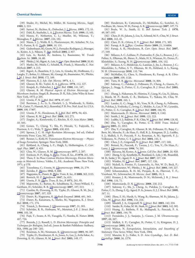
7746 dx.doi.org/10.1021/cr100353t |Chem. Rev. 2011, 111, 7710–7748
Chemical Reviews REVIEW
(39) Studer, D.; Michel, M.; M€uller, M. Scanning Microsc., Suppl.1989, 3, 253.(40) Sartori, N.; Richter, K.; Dubochet, J. J. Microsc. 1993, 172, 55.(41) Dahl, R.; Staehelin, L. A. J. Electron Microsc. Tech. 1989, 13, 165.(42) Hawes, P.; Netherton, C. L.; Mueller, M.; Wileman, T.;
Monaghan, P. J. Microsc. 2007, 226, 182.(43) Nixon, S. J.; Webb, R. I.; Floetenmeyer, M.; Schieber, N.; Lo,
H. P.; Parton, R. G. Traffic 2009, 10, 131.(44) Grabenbauer,M.; Geerts,W. J.; Fernadez-Rodriguez, J.; Hoenger,
A.; Koster, A. J.; Nilsson, T. Nat. Methods 2005, 2, 857.(45) Leis, A.; Rockel, B.; Andrees, L.; Baumeister, W. Trends
Biochem. Sci. 2009, 34, 60.(46) Plitzko, J.M.; Rigort, A.; Leis, A.Curr. Opin. Biotechnol. 2009, 20, 83.(47) Marko, M.; Hsieh, C.; Schalek, R.; Frank, J.; Mannella, C. Nat.
Methods 2007, 4, 215.(48) Rigort, A.; Bauerlein, F. J.; Leis, A.; Gruska, M.; Hoffmann, C.;
Laugks, T.; Bohm, U.; Eibauer, M.; Gnaegi, H.; Baumeister, W.; Plitzko,J. M. J. Struct. Biol. 2010, 172, 169.(49) Hanszen, K. J. Adv. Opt. Microsc. 1971, 4, 1.(50) Glaeser, R. M.; Taylor, K. A. J. Microsc. 1978, 112, 127.(51) Knapek, E.; Dubochet, J. J. Mol. Biol. 1980, 141, 147.(52) Glaeser, R. M. Physical Aspects of Electron Microscopy and
Microbeam Analysis; Siegel, B., Beaman, D. R., Eds.; John Wiley & Sons:New York, 1975; p 205.(53) Unwin, P. N. J. Mol. Biol. 1974, 87, 657.(54) Berriman, J. A.; Li, S.; Hewlett, L. J.; Wasilewski, S.; Kiskin,
F. N.; Carter, T.; Hannah,M. J.; Rosenthal, P. B. Proc. Natl. Acad. Sci. U.S.A.2009, 106, 17407.(55) Unwin, P. N.; Henderson, R. J. Mol. Biol. 1975, 94, 425.(56) Glaeser, R. M. J. Struct. Biol. 2008, 163, 271.(57) Ziegler, A.; Kisielowski, C.; Ritchie, R. O. Acta Mater. 2002,
50, 565.(58) Gonen, T.; Cheng, Y.; Sliz, P.; Hiroaki, Y.; Fujiyoshi, Y.;
Harrison, S. C.; Walz, T. Nature 2005, 438, 633.(59) Spence, J. C. H. High Resolution Microscopy, 3rd ed.; Oxford
University Press: Cary, NC, 2003.(60) Reimer, L.; Kohl, H. Transmission Electron Microscopy� Physics
of Image Formation; Springer: New-York, 2008.(61) Kirkland, A.; Chang, L.-Y.; Haigh, S.; Hetherington, C. Curr.
Appl. Phys. 2007, 8, 425.(62) Chiu, W.; Glaeser, R. M. Ultramicroscopy 1977, 2, 207.(63) Erickson, H. P.; Klug, A. Philos. Trans. R. Soc., B 1970, 261, 105.(64) Thon, F. In Phase Contrast Electron Microscopy. Electron Micro-
scopy in Materials Science; Valdre, U., Ed.; Academic Press: New York,1971; p 570.(65) Toyoshima, C.; Unwin, N. Ultramicroscopy 1988, 25, 279.(66) Zernike, F. Physica 1942, 9, 686.(67) Nagayama, K.; Danev, R. Philos. Trans. R. Soc., B 2008, 363, 2153.(68) Boersch, H. Z. Naturforsch. 1947, 2a, 615.(69) Unwin, P. N. Philos. Trans. R. Soc., B 1971, 261, 95.(70) Majorovits, E.; Barton, B.; Schultheiss, K.; Perez-Willard, F.;
Gerthsen, D.; Schr€oder, R. R. Ultramicroscopy 2007, 107, 213.(71) Cambie, R.; Downing, K. H.; Typke, D.; Glaeser, R. M.; Jin, J.
Ultramicroscopy 2007, 107, 329.(72) Danev, R.; Nagayama, K. Methods Enzymol. 2010, 481, 343.(73) Danev, R.; Kanamaru, S.; Marko, M.; Nagayama, K. J. Struct.
Biol. 2010, 171, 174.(74) Trinick, J.; Berriman, J. Ultramicroscopy 1987, 21, 393.(75) Schr€oder, R. R.; Hofmann, W.; Menetret, J.-F. J. Struct. Biol.
1990, 105, 28.(76) Fujii, T.; Iwane, A. H.; Yanagida, T.; Namba, K. Nature 2010,
467, 724.(77) Bozzola, J. J.; Russell, L. D. Electron Microscopy: Principles and
Techniques for Biologists, 2nd ed.; Jones & Bartlett Publishers: Sudbury,MA, 1998; pp 240�261.(78) Roseman, A. M.; Neumann, K. Ultramicroscopy 2003, 96, 207.(79) Typke, D.; Nordmeyer, R. A.; Jones, A.; Lee, J.; Avila-Sakar, A.;
Downing, K. H.; Glaeser, R. M. J. Struct. Biol. 2005, 149, 17.
(80) Henderson, R.; Cattermole, D.; McMullan, G.; Scotcher, S.;Fordham, M.; Amos, W. B.; Faruqi, A. R. Ultramicroscopy 2007, 107, 73.
(81) Boyle, W. S.; Smith, G. E. Bell Systems Tech. J. 1970,49, 587–593.
(82) Chen, D.H.; Jakana, J.; Liu, X.; Schmid,M. F.; Chiu,W. J. Struct.Biol. 2008, 163, 45.
(83) Clare, D. K.; Orlova, E. V. J. Struct. Biol. 2010, 171, 303.(84) Faruqi, A. R. J. Phys.: Condens. Matter 2009, 21, 314004.(85) Faruqi, A. R.; Henderson, R. Curr. Opin. Struct. Biol. 2007,
17, 549.(86) Milazzo, A. C.; Leblanc, P.; Duttweiler, F.; Jin, L.; Bouwer, J. C.;
Peltier, S.; Ellisman, M.; Bieser, F.; Matis, H. S.; Wieman, H.; Denes, P.;Kleinfelder, S.; Xuong, N. H. Ultramicroscopy 2005, 104, 152.
(87) Milazzo, A. C; Moldovan, G.; Lanman, J.; Jin, L.; Bouwer, J. C.;Klienfelder, S.; Peltier, S. T.; Ellisman, M. H.; Kirkland, A. I.; Xuong,N. H. Ultramicroscopy 2010, 110, 744.
(88) McMullan, G.; Chen, S.; Henderson, R.; Faruqi, A. R. Ultra-microscopy 2009, 109, 1126.
(89) Tietz, H. R. Microsc. Microanal. 2008, 14, 804.(90) Suloway, C.; Pulokas, J.; Fellmann, D.; Cheng, A.; Guerra, F.;
Quispe, J.; Stagg, S.; Potter, C. S.; Carragher, B. J. Struct. Biol. 2005,151, 41.
(91) Zhang, J.; Nakamura, N.; Shimizu, Y.; Liang, N.; Liu, X.; Jakana,J.; Marsh, M. P.; Booth, C. R.; Shinkawa, T.; Nakata, M.; Chiu, W.J. Struct. Biol. 2009, 165, 1.
(92) Lander, G. C.; Stagg, S. M.; Voss, N. R.; Cheng, A.; Fellmann,D.; Pulokas, J.; Yoshioka, C.; Irving, C.; Mulder, A.; Lau, P. W.; Lyumkis,D.; Potter, C. S.; Carragher, B. J. Struct. Biol. 2009, 166, 95.
(93) Mastronarde, D. Microsc. Microanal. 2003, 9, 1182.(94) Smith, J. M. J. Struct. Biol. 1999, 125, 223.(95) Ludtke, S. J.; Baldwin, P. R.; Chiu, W. J. Struct. Biol. 1999, 128, 82.(96) Zhu, Y.; Carragher, B.; Potter, C. S. IEEE Trans. Medical
Imaging 2003, 22, 1053.(97) Zhu, Y.; Carragher, B.; Glaeser, R. M.; Fellmann, D.; Bajaj, C.;
Bern, M.; Mouche, F.; de Haas, F.; Hall, R. J.; Kriegman, D. J.; Ludtke,S. J.; Mallick, S. P.; Penczek, P. A.; Roseman, A. M.; Sigworth, F. J.;Volkmann, N.; Potter, C. S. J. Struct. Biol. 2004, 145, 3.
(98) Chen, J. Z.; Grigorieff, N. J. Struct. Biol. 2007, 157, 168.(99) Boisset, N.; Penczek, P.; Taveau, J. C.; You, V.; De Haas, F.;
Lamy, J. Ultramicroscopy 1998, 74, 201.(100) B�arcena, M; Koster, A. J. Semin. Cell Dev. Biol. 2009, 20, 920.(101) Zheng, S. Q.; Keszthelyi, B.; Branlund, E.; Lyle, J. M.; Braunfeld,
M. B.; Sedat, J. W.; Agard, D. A. J. Struct. Biol. 2007, 157, 138.(102) Winkler, H. J. Struct. Biol. 2007, 157, 126.(103) Nickell, S.; F€orster, F.; Linaroudis, A.; Net, W. D.; Beck, F.;
Hegerl, R.; Baumeister, W.; Plitzko, J. M. J. Struct. Biol. 2005, 149, 227.(104) Schoenmakers, R. H. M.; Perquin, R. A.; Fliervoet, T. F.;
Voorhout, W.; Schirmacher, H. Microsc. Anal. 2005, 19, 5.(105) Kremer, J. R.; Mastronarde, D. N.; McIntosh, J. R. J. Struct.
Biol. 1996, 116, 71.(106) Mastronarde, D. N. J. Microsc. 2008, 230, 212.(107) Suloway, C.; Shi, J.; Cheng, A.; Pulokas, J.; Carragher, B.;
Potter, C. S.; Zheng, S. Q.; Agard, D. A.; Jensen, G. J. J. Struct. Biol. 2009,167, 11.
(108) Zhou, Z. H.; Hardt, S.; Wang, B.; Sherman, M. B.; Jakana, J.;Chiu, W. J. Struct. Biol. 1996, 116, 216.
(109) Mindell, J. A.; Grigorieff, N. J. Struct. Biol. 2003, 142, 334.(110) Sander, B.; Golas, M. M.; Stark, H. J. Struct. Biol. 2003, 142, 392.(111) Huang, Z.; Baldwin, P. R.; Mullapudi, S.; Penczek, P. A.
J. Struct. Biol. 2003, 144, 79.(112) Fern�andez, J. J.; Sanjurjo, J.; Carazo, J. M. Ultramicroscopy
1997, 68, 267.(113) Mallick, S. P.; Carragher, B.; Potter, C. S.; Kriegman, D. J.
Ultramicroscopy 2005, 104, 8.(114) Wiener, N. Extrapolation, Interpolation, and Smoothing of
Stationary Time Series; Wiley: New York, 1964.(115) Mancini, E. J.; Fuller, S. D. Acta Crystallogr., Sect. D: Biol.
Crystallogr. 2000, 56, 1278.
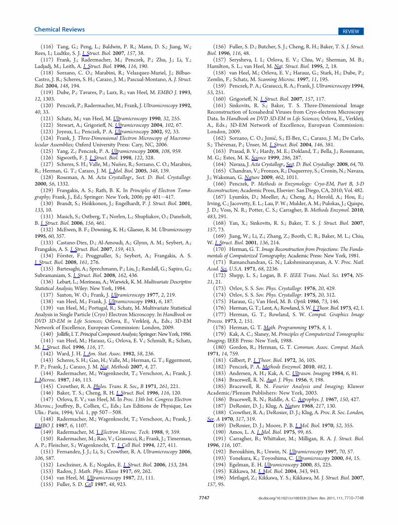
7747 dx.doi.org/10.1021/cr100353t |Chem. Rev. 2011, 111, 7710–7748
Chemical Reviews REVIEW
(116) Tang, G.; Peng, L.; Baldwin, P. R.; Mann, D. S.; Jiang, W.;Rees, I.; Ludtke, S. J. J. Struct. Biol. 2007, 157, 38.(117) Frank, J.; Radermacher, M.; Penczek, P.; Zhu, J.; Li, Y.;
Ladjadj, M.; Leith, A. J. Struct. Biol. 1996, 116, 190.(118) Sorzano, C. O.; Marabini, R.; Velazquez-Muriel, J.; Bilbao-
Castro, J. R.; Scheres, S. H.; Carazo, J. M.; Pascual-Montano, A. J. Struct.Biol. 2004, 148, 194.(119) Dube, P.; Tavares, P.; Lurz, R.; van Heel, M. EMBO J. 1993,
12, 1303.(120) Penczek, P.; Radermacher, M.; Frank, J.Ultramicroscopy 1992,
40, 33.(121) Schatz, M.; van Heel, M. Ultramicroscopy 1990, 32, 255.(122) Stewart, A.; Grigorieff, N. Ultramicroscopy 2004, 102, 67.(123) Joyeux, L.; Penczek, P. A. Ultramicroscopy 2002, 92, 33.(124) Frank, J. Three-Dimensional Electron Microscopy of Macromo-
lecular Assemblies; Oxford University Press: Cary, NC, 2006.(125) Yang, Z.; Penczek, P. A. Ultramicroscopy 2008, 108, 959.(126) Sigworth, F. J. J. Struct. Biol. 1998, 122, 328.(127) Scheres, S. H.; Valle, M.; Nu~nez, R.; Sorzano, C. O.; Marabini,
R.; Herman, G. T.; Carazo, J. M. J. Mol. Biol. 2005, 348, 139.(128) Roseman, A. M. Acta Crystallogr., Sect. D: Biol. Crystallogr.
2000, 56, 1332.(129) Frangakis, A. S.; Rath, B. K. In Principles of Electron Tomo-
graphy; Frank, J., Ed.; Springer: New York, 2006; pp 401�417.(130) Brandt, S.; Heikkonen, J.; Engelhardt, P. J. Struct. Biol. 2001,
133, 10.(131) Masich, S.; Ostberg, T.; Norlen, L.; Shupliakov, O.; Daneholt,
B. J. Struct. Biol. 2006, 156, 461.(132) McEwen, B. F.; Downing, K. H.; Glaeser, R. M. Ultramicroscopy
1995, 60, 357.(133) Castano-Diez, D.; Al-Amoudi, A.; Glynn, A. M.; Seybert, A.;
Frangakis, A. S. J. Struct. Biol. 2007, 159, 413.(134) F€orster, F.; Pruggnaller, S.; Seybert, A.; Frangakis, A. S.
J. Struct. Biol. 2008, 161, 276.(135) Bartesaghi, A.; Sprechmann, P.; Liu, J.; Randall, G.; Sapiro, G.;
Subramaniam, S. J. Struct. Biol. 2008, 162, 436.(136) Lebart, L.; Morineau, A.; Warwick, K. M.Multivariate Descriptive
Statistical Analysis; Wiley: New York, 1984.(137) Saxton, W. O.; Frank, J. Ultramicroscopy 1977, 2, 219.(138) van Heel, M.; Frank, J. Ultramicroscopy 1981, 6, 187.(139) van Heel, M.; Portugal, R.; Schatz, M. Multivariate Statistical
Analysis in Single Particle (Cryo) Electron Microscopy. InHandbook onDVD 3D-EM in Life Sciences; Orlova, E., Verkleij, A., Eds.; 3D-EMNetwork of Excellence, European Commission: London, 2009.(140) Jolliffe, I.T.PrincipalComponentAnalysis; Springer:NewYork, 1986.(141) van Heel, M.; Harauz, G.; Orlova, E. V.; Schmidt, R.; Schatz,
M. J. Struct. Biol. 1996, 116, 17.(142) Ward, J. H. J. Am. Stat. Assoc. 1982, 58, 236.(143) Scheres, S. H.; Gao, H.; Valle, M.; Herman, G. T.; Eggermont,
P. P.; Frank, J.; Carazo, J. M. Nat. Methods 2007, 4, 27.(144) Radermacher, M.; Wagenknecht, T.; Verschoor, A.; Frank, J.
J. Microsc. 1987, 146, 113.(145) Crowther, R. A. Philos. Trans. R. Soc., B 1971, 261, 221.(146) Baker, T. S.; Cheng, R. H. J. Struct. Biol. 1996, 116, 120.(147) Orlova, E. V.; van Heel, M. In Proc. 13th Int. Congress Electron
Microsc.; Jouffrey, B., Colliex, C., Eds.; Les Editions de Physique, LesUlis.: Paris, 1994; Vol. 1, pp 507�508.(148) Radermacher, M.; Wagenknecht, T.; Verschoor, A.; Frank, J.
EMBO J. 1987, 6, 1107.(149) Radermacher, M. J. Electron Microsc. Tech. 1988, 9, 359.(150) Radermacher, M.; Rao, V.; Grassucci, R.; Frank, J.; Timerman,
A. P.; Fleischer, S.; Wagenknecht, T. J. Cell Biol. 1994, 127, 411.(151) Fernandez, J. J.; Li, S.; Crowther, R. A. Ultramicroscopy 2006,
106, 587.(152) Leschziner, A. E.; Nogales, E. J. Struct. Biol. 2006, 153, 284.(153) Radon, J. Math. Phys. Klasse 1917, 69, 262.(154) van Heel, M. Ultramicroscopy 1987, 21, 111.(155) Fuller, S. D. Cell 1987, 48, 923.
(156) Fuller, S. D.; Butcher, S. J.; Cheng, R. H.; Baker, T. S. J. Struct.Biol. 1996, 116, 48.
(157) Serysheva, I. I.; Orlova, E. V.; Chiu, W.; Sherman, M. B.;Hamilton, S. L.; van Heel, M. Nat. Struct. Biol. 1995, 2, 18.
(158) van Heel, M.; Orlova, E. V.; Harauz, G.; Stark, H.; Dube, P.;Zemlin, F.; Schatz, M. Scanning Microsc. 1997, 11, 195.
(159) Penczek, P. A.; Grasucci, R. A.; Frank, J.Ultramicroscopy 1994,53, 251.
(160) Grigorieff, N. J. Struct. Biol. 2007, 157, 117.(161) Sinkovits, R. S.; Baker, T. S. Three-Dimensional Image
Reconstruction of Icosahedral Viruses from Cryo-electron MicroscopyData. In Handbook on DVD 3D-EM in Life Sciences; Orlova, E., Verkleij,A., Eds.; 3D-EM Network of Excellence, European Commission:London, 2009.
(162) Sorzano, C. O.; Joni�c, S.; El-Bez, C.; Carazo, J. M.; De Carlo,S.; Th�evenaz, P.; Unser, M. J. Struct. Biol. 2004, 146, 381.
(163) Prasad, B. V.; Hardy, M. E.; Dokland, T.; Bella, J.; Rossmann,M. G.; Estes, M. K. Science 1999, 286, 287.
(164) Navaza, J. Acta Crystallogr., Sect. D: Biol. Crystallogr. 2008, 64, 70.(165) Chandran, V.; Fronzes, R.; Duquerroy, S.; Cronin, N.; Navaza,
J.; Waksman, G. Nature 2009, 462, 1011.(166) Penczek, P. Methods in Enzymology: Cryo-EM, Part B, 3-D
Reconstruction; Academic Press, Elsevier: San Diego, CA, 2010; Vol. 482.(167) Lyumkis, D.; Moeller, A.; Cheng, A.; Herold, A.; Hou, E.;
Irving, C.; Jacovetty, E. L.; Lau, P.W.;Mulder, A.M.; Pulokas, J.; Quispe,J. D.; Voss, N. R.; Potter, C. S.; Carragher, B. Methods Enzymol. 2010,483, 291.
(168) Yan, X.; Sinkovits, R. S.; Baker, T. S. J. Struct. Biol. 2007,157, 73.
(169) Jiang, W.; Li, Z.; Zhang, Z.; Booth, C. R.; Baker, M. L.; Chiu,W. J. Struct. Biol. 2001, 136, 214.
(170) Herman, G. T. Image Reconstruction from Projections: The Funda-mentals of Computerized Tomography; Academic Press: New York, 1981.
(171) Ramanchandran, G. N.; Lakshminarayanan, A. V. Proc. Natl.Acad. Sci. U.S.A. 1971, 68, 2236.
(172) Shepp, L. S.; Logan, B. F. IEEE Trans. Nucl. Sci. 1974, NS-21, 21.
(173) Orlov, S. S. Sov. Phys. Crystallogr. 1976, 20, 429.(174) Orlov, S. S. Sov. Phys. Crystallogr. 1975, 20, 312.(175) Harauz, G.; Van Heel, M. B. Optik 1986, 73, 146.(176) Herman, G. T.; Lent, A.; Rowland, S.W. J. Theor. Biol. 1973, 42, 1.(177) Herman, G. T.; Rowland, S. W. Comput. Graphics Image
Process. 1973, 2, 151.(178) Herman, G. T. Math. Programming 1975, 8, 1.(179) Kak, A. C.; Slaney, M. Principles of Computerized Tomographic
Imaging; IEEE Press: New York, 1988.(180) Gordon, R.; Herman, G. T. Commun. Assoc. Comput. Mach.
1971, 14, 759.(181) Gilbert, P. J. Theor. Biol. 1972, 36, 105.(182) Penczek, P. A. Methods Enzymol. 2010, 482, 1.(183) Andersen, A. H.; Kak, A. C. Ultrason. Imaging 1984, 6, 81.(184) Bracewell, R. N. Aust. J. Phys. 1956, 9, 198.(185) Bracewell, R. N. Fourier Analysis and Imaging; Kluwer
Academic/Plenum Publishers: New York, 2003.(186) Bracewell, R. N.; Riddle, A. C. Astrophys. J. 1967, 150, 427.(187) DeRosier, D. J.; Klug, A. Nature 1968, 217, 130.(188) Crowther, R. A.; DeRosier, D. J.; Klug, A. Proc. R. Soc. London,
Ser. A 1970, 317, 319.(189) DeRosier, D. J.; Moore, P. B. J. Mol. Biol. 1970, 52, 355.(190) Amos, L. A. J. Mol. Biol. 1975, 99, 65.(191) Carragher, B.; Whittaker, M.; Milligan, R. A. J. Struct. Biol.
1996, 116, 107.(192) Beroukhim, R.; Unwin, N. Ultramicroscopy 1997, 70, 57.(193) Yonekura, K.; Toyoshima, C. Ultramicroscopy 2000, 84, 15.(194) Egelman, E. H. Ultramicroscopy 2000, 85, 225.(195) Kikkawa, M. J. Mol. Biol. 2004, 343, 943.(196) Metlagel, Z.; Kikkawa, Y. S.; Kikkawa, M. J. Struct. Biol. 2007,
157, 95.
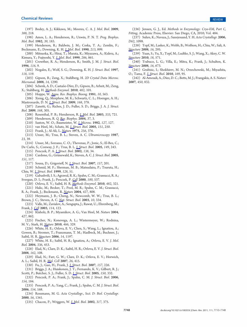
7748 dx.doi.org/10.1021/cr100353t |Chem. Rev. 2011, 111, 7710–7748
Chemical Reviews REVIEW
(197) Bodey, A. J.; Kikkawa, M.; Moores, C. A. J. Mol. Biol. 2009,388, 218.(198) Amos, L. A.; Henderson, R.; Unwin, P. N. T. Prog. Biophys.
Mol. Biol. 1982, 39, 183.(199) Henderson, R.; Baldwin, J. M.; Ceska, T. A.; Zemlin, F.;
Beckmann, E.; Downing, K. H. J. Mol. Biol. 1990, 213, 899.(200) Mitsuoka, K.; Hirai, T.; Murata, K.; Miyazawa, A.; Kidera, A.;
Kimura, Y.; Fujiyoshi, Y. J. Mol. Biol. 1999, 286, 861.(201) Crowther, R. A.; Henderson, R.; Smith, J. M. J. Struct. Biol.
1996, 116, 9.(202) Nogales, E.; Wolf, S. G.; Downing, K. H. J. Struct. Biol. 1997,
118, 119.(203) Gipson, B.; Zeng, X.; Stahlberg, H. 2D Crystal Data Microsc.
Microanal. 2008, 14, 1290.(204) Schenk, A. D.; Casta~no-Díez, D.; Gipson, B.; Arheit, M.; Zeng,
X.; Stahlberg, H. Methods Enzymol. 2010, 482, 101.(205) Hoppe, W. Annu. Rev. Biophys. Bioeng. 1981, 10, 563.(206) Xiong, Q.; Morphew, M. K.; Schwartz, C. L.; Hoenger, A. H.;
Mastronarde, D. N. J. Struct. Biol. 2009, 168, 378.(207) Zanetti, G.; Riches, J. D.; Fuller, S. D.; Briggs, J. A. J. Struct.
Biol. 2009, 168, 305.(208) Rosenthal, P. B.; Henderson, R. J. Mol. Biol. 2003, 333, 721.(209) Henderson, R. Q. Rev. Biophys. 2004, 37, 3.(210) Saxton, W. O.; Baumeister, W. J. Microsc. 1982, 127, 127.(211) van Heel, M.; Schatz, M. J. Struct. Biol. 2005, 151, 250.(212) Frank, J.; Al-Ali, L. Nature 1975, 256, 376.(213) Unser, M.; Trus, B. L.; Steven, A. C. Ultramicroscopy 1987,
23, 39.(214) Unser, M.; Sorzano, C. O.; Thevenaz, P.; Jonic, S.; El-Bez, C.;
De Carlo, S.; Conway, J. F.; Trus, B. L. J. Struct. Biol. 2005, 149, 243.(215) Penczek, P. A. J. Struct. Biol. 2002, 138, 34.(216) Cardone, G.; Gr€unewald, K.; Steven, A. C. J. Struct. Biol. 2005,
151, 117.(217) Sousa, D.; Grigorieff, N. J. Struct. Biol. 2007, 157, 201.(218) Schmid, M. F.; Sherman, M. B.; Matsudaira, P.; Tsuruta, H.;
Chiu, W. J. Struct. Biol. 1999, 128, 51.(219) Gabashvili, I. S.; Agrawal, R. K.; Spahn, C.M.; Grassucci, R. A.;
Svergun, D. I.; Frank, J.; Penczek, P. Cell 2000, 100, 537.(220) Orlova, E. V.; Saibil, H. R. Methods Enzymol. 2010, 482, 321.(221) Halic, M.; Becker, T.; Pool, M. R.; Spahn, C. M.; Grassucci,
R. A.; Frank, J.; Beckmann, R. Nature 2004, 427, 808.(222) Heymann, J. B.; Cheng, N.; Newcomb, W. W.; Trus, B. L.;
Brown, J. C.; Steven, A. C. Nat. Struct. Biol. 2003, 10, 334.(223) Valle, M.; Zavialov, A.; Sengupta, J.; Rawat, U.; Ehrenberg, M.;
Frank, J. Cell 2003, 114, 123.(224) Klaholz, B. P.; Myasnikov, A. G.; Van Heel, M. Nature 2004,
427, 862.(225) Fischer, N.; Konevega, A. L.; Wintermeyer, W.; Rodnina,
M. V.; Stark, H. Nature 2010, 466, 329.(226) White, H. E.; Orlova, E. V.; Chen, S.; Wang, L.; Ignatiou, A.;
Gowen, B.; Stromer, T.; Franzmann, T. M.; Haslbeck, M.; Buchner, J.;Saibil, H. R. Structure 2006, 14, 1197.(227) White, H. E.; Saibil, H. R.; Ignatiou, A.; Orlova, E. V. J. Mol.
Biol. 2004, 336, 453.(228) Elad, N.; Clare, D. K.; Saibil, H. R.; Orlova, E. V. J. Struct. Biol.
2008, 162, 108.(229) Elad, N.; Farr, G. W.; Clare, D. K.; Orlova, E. V.; Horwich,
A. L.; Saibil, H. R. Mol. Cell 2007, 26, 415.(230) Fu, J.; Gao, H.; Frank, J. J. Struct. Biol. 2007, 157, 226.(231) Briggs, J. A.; Huiskonen, J. T.; Fernando, K. V.; Gilbert, R. J.;
Scotti, P.; Butcher, S. J.; Fuller, S. D. J. Struct. Biol. 2005, 150, 332.(232) Penczek, P. A.; Frank, J.; Spahn, C. M. J. Struct. Biol. 2006,
154, 184.(233) Penczek, P. A.; Yang, C.; Frank, J.; Spahn, C. M. J. Struct. Biol.
2006, 154, 168.(234) Rossmann, M. G. Acta Crystallogr., Sect. D: Biol. Crystallogr.
2000, 56, 1341.(235) Chacon, P.; Wriggers, W. J. Mol. Biol. 2002, 317, 375.
(236) Jensen, G. J., Ed. Methods in Enzymology: Cryo-EM, Part C,Fitting; Academic Press, Elsevier: San Diego, CA, 2010; Vol. 484.
(237) Suhre, K.; Navaza, J.; Sanejouand, Y. H.Acta Crystallogr. 2006,D62, 1098.
(238) Topf, M.; Lasker, K.; Webb, B.; Wolfson, H.; Chiu, W.; Sali, A.Structure 2008, 16, 295.
(239) Yuan, S.; Yu, X.; Topf, M.; Ludtke, S. J.; Wang, X.; Akey, C.W.Structure 2010, 18, 571.
(240) Trabuco, L. G.; Villa, E.; Mitra, K.; Frank, J.; Schulten, K.Structure 2008, 16, 673.
(241) Grubisic, I.; Shokhirev, M. N.; Orzechowski, M.; Miyashita,O.; Tama, F. J. Struct. Biol. 2010, 169, 95.
(242) Al-Amoudi, A.; Díez, D. C.; Betts, M. J.; Frangakis, A. S.Nature2007, 450, 832.