Embed Size (px)
Citation preview

ORI GIN AL PA PER
Stress Measurement by Overcoring at Shallow Depthsin a Rock Slope: the Scattering of Input Dataand Results
C. Clement Æ V. Merrien-Soukatchoff Æ C. Dunner ÆY. Gunzburger
Received: 28 March 2008 / Accepted: 13 October 2008 / Published online: 3 December 2008
� Springer-Verlag 2008
Abstract This paper describes a field experiment of stress measurement using the
overcoring method performed in a rock slope, called Rochers de Valabres (located
in France’s Southern Alps Region), a field laboratory site prone to rockfalls. Six
measurements were conducted at shallow depths from the surface, moving deeper
along a sub-horizontal borehole. The experiment was conducted in heterogeneous
and anisotropic gneiss, with the overcored rock elastic properties, as evaluated by
biaxial and uniaxial tests, being widely scattered. Since stress calculations are
sensitive to all input data uncertainties, strain inversion was, thus, performed using
an experimental device and Monte Carlo simulations. The experimental device
allows the assessment of rather broad confidence intervals for both stress magnitude
and orientation. The results indicate that the stress state in the surface area is quite
heterogeneous and may be correlated with topography. The measurements show a
nonlinear stress distribution with distance to the free surface, along with high values
of principal stresses, despite the vicinity of the surface. Although influenced by local
topography, orientations of the principal computed stresses are characterized by a
high turnover due to local heterogeneities. The results are roughly in accordance to a
2D finite element model of the site.
C. Clement (&)
LAEGO-INERIS, Nancy-Universite, Parc de Saurupt, CS 14234, 54042 Nancy, France
e-mail: [email protected]
Present Address:C. Clement
ANTEA, 1, rue du parc de Brabois, 54500 Vandoeuvre, France
V. Merrien-Soukatchoff � Y. Gunzburger
LAEGO, Nancy-Universite, Parc de Saurupt, CS 14234, 54042 Nancy, France
C. Dunner
Institut National de l’Environnement Industriel et des Risques (INERIS),
Parc de Saurupt, CS 14234, 54042 Nancy, France
123
Rock Mech Rock Eng (2009) 42:585–609
DOI 10.1007/s00603-008-0019-8

Keywords Stress � Overcoring � Rock slope � Uncertainty � Numerical modeling �Experimental device
1 Introduction
Rock slope stability is governed by several factors, including slope topography,
fracture network, groundwater pressure, seismic activity, and in situ stress
conditions. This last factor, yielding, for example, an unbalanced stress concen-
tration, can produce phenomena such as rockfalls and slipping (Amadei and
Stephansson 1997, p. 51). Panthi and Nilsen (2006) revealed that very anisotropic
stresses near the topographic surface exert a significant impact on both present and
future slope stability. Similarly, Obara et al. (2000) demonstrated that the horizontal
stress component plays a key role in estimating rock slope stability.
Even though the stress state constitutes an important factor of slope stability, it
remains difficult to grasp in the case of an irregular ground surface. As opposed to
studies on tunnels and ground-related problems, few analytical solutions of initial
stresses are available, and these are limited to smooth surfaces (Ling 1947;
Akhpatelov and Ter-Martirosyan 1971; Pan and Amadei 1994). For irregular and
complex three-dimensional topographies, numerical computations provide the best
alternative for computing in situ stresses, yet, input data are required. Stress
measurements on slopes also prove to be rare, particularly close to the surface.
Some such efforts have been performed on manmade cuts, e.g., open-pit mines and
dumps (Obara et al. 2000; Bozzano et al. 2006; Demin et al. 2003; Kang et al.
2002). However, these measurements were conducted on slopes with regular and
simple topographies and not on natural slopes.
Under these complex conditions, in situ stress measurements, by use of the
overcoring method, were performed within the experimental zone of a natural slope
called Rochers de Valabres.
Although not directly linked to instability evaluations, the stress measurement
analysis described herein is intended to:
• Offer an order of magnitude for the stress state at shallow depths, as necessary
for conducting a stability evaluation. It was decided to investigate and monitor
the surface zone of the slope (first few meters of depth) inasmuch as rockfalls
begin with a slip of the surface block (5–10 m wide). This subsurface area is
also particularly sensitive to the topographic surface, fracturation, and thermal
stresses, all of which produce a more heterogeneous and complex stress state
than for stresses inside the rock mass (Haimson 1979; Amadei and Stephansson
1997, p. 14, 108).
• Compare stress-to-stress variations due to thermal effects, which are partially
measured by a strain cell network at the Rochers de Valabres rock slope
(Merrien-Soukatchoff et al. 2007; Clement et al. 2008).
• Compare in situ measurements and their uncertainties with analytical and
numerical computations.
• Contrast measurement data with the a priori assumptions adopted for the stress
state on the rock slope. As an example, it is generally assumed that stresses close
586 C. Clement et al.
123

to the surface are smaller, since the shallower part of the slope may be less
compressed than the deeper part, due to the presence of open discontinuities and
weathering near the topographic surface (Comite Francais de Mecanique des
Roches 2004, p. 350). It may also be considered that the vertical normal stress
equals the weight of the overlying rock for horizontal topography; in the case of
hilly terrain, this evaluation would involve the orientations of the major
principal stresses lying in the plane of the slope, with the minor stresses being
normal to the slope and equal to zero. Similarly, these stresses approach zero
where the rock slope is convex upward, but increase where the slope is concave
upward (Goodman 1980, pp. 104–105, see Fig. 1).
• Evaluate the feasibility of stress measurements using the overcoring test in a
rock slope. The field experiment is, indeed, intended to apply the overcoring
technique to investigating other fractured rock slopes.
This paper will initially present the laboratory site and provide a description of
the experimental setup. A description of the drilling campaign and acquisition of
anisotropic rock properties will be described next. In order to evaluate the impact of
uncertainties and quantify errors in the estimation of in situ principal stresses, a
procedure relying upon reliability analysis (or an ‘‘experimental device’’) will be
suggested. Lastly, the stress measurement results will be detailed, discussed, and
compared with the output from a simple 2D finite element model.
2 Site Description
The Rochers de Valabres is a large fractured rock slope located in the Tinee Valley
(in France’s Southern Alps region). The slope overhangs a road, its viaduct, and a
hydroelectric power plant (Fig. 2).
Two rockfalls occurred, respectively in May 2000 (involving some 2,000 m3 of
material) and October 2004 (roughly 30 m3 of material).
Since 2002, this slope has been investigated as a laboratory site by the Laego and
Ineris Institutes (Gunzburger 2004; Gunzburger et al. 2005; Merrien-Soukatchoff
et al. 2005; Dunner et al. 2007) and the Geosciences Azur and Geosciences
Fig. 1 Estimated initial stresses in the case of a valley side, according to Goodman (1980, pp. 104–105)
Stress Measurement by Overcoring at Shallow Depths in a Rock Slope 587
123

Besancon laboratories. Beginning in 2006 and within the framework of a French
national program (entitled STABROCK), these research organizations, along with
new partners, have been concentrating their efforts on field observations,
monitoring, and numerical modeling. The scientific investigations have sought to
better understand the effect of climatic variations on rock slope stability, as well as
to test and introduce new equipment and monitoring techniques (Senfaute et al.
2006). Instrumentation technologies, such as microseismic networks, mechanical
measurements using tiltmeters, and deformations cells, have been installed in a zone
denoted the experimental area (Fig. 3). Stress measurements have been carried out
beneath this area, thanks to the presence of a former access road.
This experimental zone ranges in elevation from 700 to 900 m, with an average
dip of around 50–70�. The top of the slope actually culminates at more than
2,000 m, while the bottom of the valley lies at an altitude of 600 m.
The site is cut into hard migmatic gneiss, which displays significant foliation,
generally oriented N110�–140�E. The fracture network cuts the rock mass into
many blocks potentially capable of sliding towards the valley by means of plane
sliding (Gunzburger 2004; Gunzburger et al. 2005).
3 Stress Measurements Using the Overcoring Test
3.1 Description of Field Experiments
Overcoring methods are commonly applied with success in mine settings (Lahaie
et al. 2003), natural gas storage (Glamheden and Curtis 2006), and radioactive waste
storage research (Heusermann et al. 2003). This technique enables measurement of
the full 3D stress tensor from a single measurement; in the case of several tests
along a profile, both the stress gradients and local heterogeneous stress fields can be
detected. The scale of rock volume covered by such measurements amounts to
Fig. 2 Location of the Rochers de Valabres experimental site in the Southern French Alps
588 C. Clement et al.
123

around 10-2–10-3 m3 (Amadei and Stephansson 1997 p. 96; Bertrand 2001). The
overcoring test, thus, yields a fine level of stress tensor detail.
In November 2005, in situ stress measurements were performed by INERIS along
a sub-horizontal borehole drilled towards the north on the former road beneath the
monitored area (Dunner et al. 2007). The stress field was determined by overcoring
CSIRO Hi 12 stress cells on six locations at the following depths from the free
surface: 2.45, 4.35, 6.35, 10.25, 15.75, and 18.35 m (Fig. 4). These locations
correspond to overlying rock extending between 15 and 45 m.
Each cell comes equipped with 12 gauges (Worotnicki 1993): two axial gauges
(ez), five tangential gauges (eh), and five inclined strain gauges (e45 and e135).
During the measurement procedure, a CSIRO strain cell placed in a small-diameter
pilot hole (38 mm) is overcored by drilling a large-diameter borehole (146 mm).
The overcored sample becomes totally isolated and relieved of the surrounding
stress. The 12 strain gauges then record deformations as a result of the volume
increase in the sample created by the stress relief (Amadei 1983). The stress tensor
is calculated, using inversion methods, from the strain response and elastic
Fig. 3 Description of the experimental area of the Rochers de Valabres study slope
Stress Measurement by Overcoring at Shallow Depths in a Rock Slope 589
123

properties of the overcored sample, which are typically evaluated using biaxial tests.
The strain responses of the CSIRO cells were recorded by a SYTGEO� system and
the inversion was performed with the SYTGEOstress� software developed by
INERIS.
The stress measurement depths were chosen by virtue of the local geological
setting, i.e., fracturation rate. The first several meters of rocks from the borehole
were too heavily fractured and constrained the initial measurement conducted at a
depth of 2.5 m.
Strain curves recorded during overcoring Tests 1–6 are shown in Fig. 5, which
plots measured strain versus time. All strain curves reveal a gradual elongation and
the various types of gauges are well distinguished.
3.2 Geological Setting of the Boreholes
All 18-m samples from the borehole were investigated and described in order to
survey fractures, foliation orientation, and weathering zones. The foliation
orientation actually constitutes an input data element for strain inversion, and the
fractured or weathering zones may influence the in situ stress state. Moreover, thin
sections were prepared from each overcored sample and then investigated under the
microscope.
Fig. 4 Location of the six stress measurements within the horizontal borehole over a cross-section
590 C. Clement et al.
123

The discontinuities display a perpendicular direction with respect to the drilling
direction, varying from approximately N70� to N110�, with a dip in the 50–70%
range. This fracturation system shows good agreement with the main fracture sets,
as described on the slope scale (Gunzburger et al. 2005). These natural
discontinuities present rough, weathered, and oxidized surfaces; some discontinu-
ities contain calcite filling.
The petrological description reveals that the borehole was drilled through a
migmatic paragneiss formation, belonging to the Alpine Hercynian basement. The
rock is composed of quartz, feldspar, and mica (mostly biotite). At the slope scale,
foliation is oriented 110�–140�NE, with a dip of 65�N. On the drilling scale
however, foliation layers are undulating and often discontinuous, with quartz-
Fig. 5 Response curves observed during overcoring Tests 1–6. The dark curves with squares correspondto transverse gauges, the gray curves with triangles to inclined gauges, and the gray curves with circles toaxial gauges
Stress Measurement by Overcoring at Shallow Depths in a Rock Slope 591
123

feldspar lenses included in the host gneiss. Consequently, gneiss samples of each
overcoring test appear to be heterogeneous, and it is difficult to accurately display
the main foliation orientations of each sample. This difficulty will exert a certain
impact on stress calculations, as will be discussed further below.
Although the borehole samples exhibit numerous heterogeneities, it is still
possible to separate the drilling length into five sections (see Fig. 6) as follows:
• First section—between 1 and 8.5 m: zone with undulating foliation layers,
quartz-feldspar lenses, and quartz veins.
• Second section—between 8.5 and 11.5 m: zone with regular and thin foliation
layers dipping towards the southeast. Higher proportion of mica.
• Third section—between 11.5 and 15.5 m: zone with considerable open
fracturing, plus calcified and rough surfaces. Quartz-feldspar lenses are larger
and numerous. The foliation orientation is, therefore, imperceptible.
• Fourth section—between 15.5 and 16.5 m: known as the breccia area. Gneiss
stones are enclosed by a chlorite matrix.
• Fifth section—between 16.5 and 18.5 m: a zone similar to the first section.
3.3 Overcored Rock Mechanics Properties
The stress tensor is calculated from the strain response recorded during the
overcoring test and from the elastic parameters of overcored rock.
Since the rock fabric is clearly anisotropic, mechanical behavior will be assessed
by means of transversely isotropic theory (Amadei 1996), which requires defining
five elastic parameters: E1 and E2, Young’s moduli in the direction normal to the
plane of transverse isotropy and in the parallel direction; v12 and v23, Poisson’s ratio;
and G12, the shear modulus.
If anisotropy were to be neglected, a major error in the calculated principal
stresses would be introduced (Amadei and Stephansson 1997, pp. 108–109). Hooker
and Johnson (1969) derived an error of approximately 25% in magnitude and 25� in
orientation, while Amadei (1996) and then Lahaie (2005) demonstrated that
anisotropy can introduce 33 and 40% error, respectively.
Fig. 6 Location of overcoring tests and the petrological sections
592 C. Clement et al.
123

Elastic parameters are typically obtained from biaxial testing applied directly on
the overcored sample. In our case however, biaxial tests were not sufficient to
estimate the entire transversely isotropic elastic matrix. It proved necessary to use
uniaxial testing for a full determination of anisotropic properties. Given that the
rock is clearly anisotropic and heterogeneous and that various types of laboratory
tests were employed, the elastic parameters are widely scattered and affected by
uncertainties, as will be shown below.
3.3.1 Biaxial Testing
In this paper, the so-called biaxial test designates the test directly performed on the
overcored sample using a biaxial chamber. A radial and increasing confining
pressure is to be applied, although no prescribed load or displacement is applied on
the sample axis.
Only two overcored samples (120 mm diameter and 600 mm long), retrieved
from a depth of 2.45 m (Test 1) and 15.75 m (Test 5), were usable for the biaxial
tests. Indeed, the length of the overcored samples extracted from Tests 2, 3, 4, and 6
were too short to be introduced in the biaxial chamber.
The Test 1 sample clearly exhibits a foliation plane, hence, an anisotropic
fabric, while the second sample (Test 5) is composed of breccia and will be
considered as isotropic. Two loading–unloading cycles were introduced on each
sample.
Nevertheless, biaxial testing can only establish the apparent elastic parameters,
i.e., Young’s modulus (Eeq) and Poisson’s ratio (veq), with the assumption of an
isotropic material. The results are shown in Table 1.
Table 1 shows low Poisson’s ratio values, especially for Test 5, and a scattering
of the apparent Young’s modulus values, which may be caused by both anisotropy
and heterogeneity at the sample scale.
In the case of the Test 1 sample however, i.e., for an anisotropic sample, biaxial
testing is not sufficient to estimate all of the transversely isotropic parameters (E1,
E2, v12, v23, and G12), since this testing is not being performed in the plane of
foliation or normal to it and since, to the best of our knowledge, no analytical
solutions have actually been proposed for such a complete determination by means
of biaxial testing.
Table 1 Apparent elastic parameters calculated during biaxial testing
Apparent elastic parameter Minimum Maximum Mean Standard deviation
Test 1
Eeq: Young’s modulus (GPa) 18.2 33.6 27.5 5.6
veq: Poisson’s ratio 0.06 0.19 0.12 0.07
Test 5
Eeq: Young’s modulus (GPa) 23.1 42.1 29.7 7.8
veq: Poisson’s ratio 0.05 0.06 0.05 0.003
Stress Measurement by Overcoring at Shallow Depths in a Rock Slope 593
123

3.3.2 Uniaxial Testing
In order to estimate the transversely isotropic parameters, uniaxial compression tests
were conducted on specimens cut at different angles with respect to the plane of
transverse isotropy. Two samples were collected from the borehole at depths of 2.88
and 15.5 m, and then cut into eight specimens (38 mm in diameter and 76 mm long)
and instrumented with strain gauges. All of the specimens displayed foliation layers
and were considered to be anisotropic.
The five independent elastic properties (i.e., E1, E2, v12, v23, and G12) were
determined from the linear portion of stress–strain curves via several loading–
unloading cycles. The results from uniaxial compression tests indicate a clearly
anisotropic fabric with an anisotropy factor (R = E2/E1) of about 1.4. The entire set
of transversely isotropic parameters, measured at a point 2.88 m deep, is presented
in Table 2.
3.3.3 Choice of Mechanical Parameters
Two kinds of laboratory tests were conducted on Valabres samples at two different
scales; this approach has served to raise the problem of parameter value choice
inherent in this study.
Biaxial testing can only determine the apparent elastic parameters, i.e., Young’s
modulus (Eeq) and Poisson’s ratio (veq), under the assumption of an isotropic
material. Biaxial testing does, however, yield an order of magnitude for
mechanical parameters at the scale of the overcoring test, given that the samples
are directly extracted from the in situ experiment and correspond to the scale of
the studied volume (i.e., around 10-2–10-3 m3, Bertrand 2001) and its state of
heterogeneities. These apparent elastic parameters must be kept to follow up with
the study.
On the other hand, uniaxial tests are carried out on smaller specimens, which do
not correspond to the scale of the studied rock volume. They are, however, useful in
quantifying rock anisotropy by being performed with reference to the plane of
transverse isotropy.
Consequently, we decided to deduce the transversely isotropic parameters E1 and
E2 using apparent parameters from biaxial testing (due to their scale), along with the
anisotropic factor R from uniaxial testing. We also decided to maintain the
anisotropic Poisson’s ratio.
Table 2 Transversely isotropic parameters calculated from uniaxial testing at a point 2.88 m deep
Transversely isotropic
parameter
Minimum Maximum Mean Standard
deviation
Number
of values
E1 (GPa) 32.2 48.50 41 5.2 7
E2 (GPa) 56.20 60.37 58 1.5 4
v12 0.09 0.15 0.13 0.02 7
v23 0.12 0.17 0.15 0.02 4
G12 (GPa) 20 1
594 C. Clement et al.
123

4 Stress Computations with the Experimental Device
4.1 Understanding and the Handling of Uncertainties: use of the Experimental
Device
Stress computations by means of strain inversion require input data, such as
mechanical parameters and (two-angle) foliation orientation in the case of a
transversely isotropic material. If these parameters are known, then the
knowledge of strain after overcoring will lead to determining the stress tensor
by inversion and least-squares minimization. In our case, the determination of
these input data was complex and involved several sources of uncertainties, as
detailed below:
• Uncertainties on foliation layer orientation, due to undulating foliation.
• A scattering of mechanical properties, which could be caused by the
considerable heterogeneity of the gneiss sample, as revealed during the
petrological description of the borehole.
• Uncertainties on anisotropic elastic properties, due to the use of two kinds of
laboratory tests at various scales.
• Uncertainties on elastic properties of overcoring Tests 2, 3, 4, and 6. Biaxial
and uniaxial testing was performed at just two locations (overcoring Tests 1
and 5), and their elastic rock properties will be extrapolated to the other
points.
The first two points correspond to the natural spatial variability of the rock, while
the last two correspond to measurement uncertainties.
Stress computations however, are sensitive to all input data uncertainties, which
cannot be overcome, though it is possible to quantify their impact by displaying
results with a confidence interval evaluation.
In our specific case, we have decided to perform a reliability analysis (also called
‘‘experimental device’’). Both mechanical and geometric input data are treated as
random variables, according to Monte Carlo analysis techniques, and their influence
on the output random variable will be examined.
This process can be detailed as follows (see Fig. 7):
• Input data are mechanical parameters and geometric characteristics (azimuth
and dip of the foliation layer); they are generated using Monte Carlo
simulations. The random intervals are chosen with respect to variations deduced
from laboratory testing and sample observation.
• Output data are stress tensors, i.e., magnitude, azimuth, and dip angle. Using
random input data, the strain data inversion produced 500 stress tensors for each
Fig. 7 Summary diagram of the experimental device
Stress Measurement by Overcoring at Shallow Depths in a Rock Slope 595
123

measurement point. Such an inversion was performed using the SYTGEO-
Stress� software application (Lahaie and Renaud 2005).
• The impact of uncertainties may be assessed both qualitatively with response
surface models and quantitatively with multiple regression operations.
• The stress estimation can then be presented, together with confidence intervals,
and interpreted more accurately.
Such statistical techniques, e.g., least-squares method and Monte Carlo
analysis, have already been used successfully by Cornet and Valette (1984) and
by Walter et al. (1990); they may be applied to stress determination using
hydraulic fracturing. These methods produce a variation domain and, with it,
confidence intervals on the magnitude and orientation of the mean principal
stresses. The level of confidence assigned to stress determination will then provide
an order of magnitude for the resolution needed when performing numerical
modeling.
4.2 Random Input Data Intervals
The quality and precision of the experimental device depends on the choice of
random input data intervals; in our case, the input data will depend on mechanical
behavior, i.e.:
• For an isotropic material, i.e., for overcored Test 5, only two input data are
necessary: E, Young’s modulus; and v, Poisson’s ratio.
• For a transversely isotropic material, i.e., for overcored Tests 1, 2, 3, 4, and 6,
five mechanical properties (E1, E2, v12, v23, and G12) and two geometric
parameters (azimuth [A] and dip [D] of the foliation layers) need to be
introduced. These five mechanical properties have been reduced to three
(R = E2/E1, v12, v23) using:
• A Saint-Venant approximation (Amadei 1996):
1
G12
¼ 1þ 2v12
E1
þ 1
E2
ð1Þ
• A fixed value of Eeq (i.e., 27.5 GPa) and an assumption between E1 and E2,
the anisotropy factor R, and Eeq.
Furthermore, since only two measurement points (Tests 1 and 5) were
characterized using laboratory results, it proved necessary to extrapolate rock
properties to the other measurement points. Transversely, isotropic parameters
obtained during Test 1 have, thus, been applied to Tests 2, 3, 4, and 6, which reveal
anisotropic behavior and apparent foliation layers. Only Test 5 is considered to be
isotropic.
The mechanical parameter random intervals for each overcored test are listed in
Table 3. The intervals for each mechanical parameter have been deduced from the
maximum and minimum values yielded by laboratory testing.
596 C. Clement et al.
123

Foliation layers (two parameters: azimuth [A] and dip [D]) are also random. Their
intervals depend on the irregularity observed in borehole samples.
4.3 Results: Application of the Experimental Device on Overcored Test 1
The experimental device will be detailed first on overcored Test 1 in order to clarify
the method. Explanations will focus on the major principal stress (r1). The aim here
is to bound the major principal stress magnitude (m_r1), trend (tr_r1), and plunge
(pl_r1), all of which depend upon random input data by use of regression analysis. A
polynomial equation connecting the output (m_r1, tr_r1, and pl_r1) with five input
variables (R, v12, v23, A, and D) can be derived according to the following equation:
y ¼ b0 þ b1Rþ b2v12 þ b3v23 þ b4Aþ b5D ð2Þ
where y is one of the output parameters (m_r1, tr_r1, or pl_r1) and b0, b1, b2,... are
the regression coefficients, which may be considered as a weighting of the influence
from each input parameter.
Let’s note that the multiple linear regression analysis is performed on a
standardized database (i.e., with a reduced centered variable).
In order to ensure model adequacy, the multiple determination coefficient (R2) is
calculated for each regression analysis using the following expression:
R2 ¼Pn
i¼1 yi � �yð Þ2Pn
i¼1 yi � �yð Þ2ð3Þ
where �y; yi, and yi are the mean, the real values, and the predicted values of the
output response (y), respectively. R2 lies between 0 and 1, with a value close to 1
indicating that the majority of the variability in y is explained by the regression
analysis. Table 4 presents, for each output data element, the regression coefficient
for each input parameter and the corresponding R2 values.
The above table reveals that the variation in output response stems from a
complex combination of input data, i.e.:
• The magnitude of r1 is more heavily influenced by mechanical parameters.
Anisotropy factor R is especially influential.
• The variation in r1 trend is bounded with anisotropy factor R and foliation layer
dip D. v23 also exerts a significant impact.
Table 3 Random mechanical
parameter intervalsMechanical parameter Minimum Maximum
Tests 1, 2, 3, 4, and 6 (transversely isotropic)
R = E2/E1 1.16 1.9
v12 0.06 0.19
v23 0.12 0.17
Test 5 (isotropic)
E (GPa) 23.1 42.1
v 0.05 0.06
Stress Measurement by Overcoring at Shallow Depths in a Rock Slope 597
123

• The variation in plunge r1 depends on both v23 and the geometric parameters (Aand D).
• The high R2 values suggest good model approximation.
Furthermore, the response surface representation may be used to analyze
response variability versus the random input parameters. Figure 8 depicts the
variability in r1 magnitude versus both anisotropy factor R and Poisson’s ratio v12.
It can be observed that the magnitude of r1 increases with higher R values and then
decreases with higher v12 values.
Moreover, application of the experimental device on Test 1 has produced an
estimation of r1, along with its variability and, hence, its confidence interval:
• The mean magnitude of r1 is 6.3 MPa, with a standard deviation of ±0.8 MPa.
• The mean trend of r1 is 290�N, with a standard deviation of ±15�. In comparison
with the potential trend range (360�), this variability becomes minor.
• The mean plunge of r1 is 56�, with a standard deviation of ±15�.
The directions of the three principal stresses calculated for overcoring Test 1,
using the experimental device, have been plotted on the lower-hemisphere polar
stereographic projection (OX: north, OY: upward vertical, OZ: east) in Fig. 9.
Fig. 8 Response surface for a magnitude of r1 versus both v12 and R
Table 4 Results from the linear regression analysis: calculation of regression coefficients
Constant R = E2/E1 v12 v23 A D R2
m_r1 -0.11 0.62 20.46 0.30 -0.13 0.02 0.98
tr_r1 0.49 20.39 -0.04 20.15 -0.02 20.80 0.96
pl_r1 -0.13 0.01 -0.05 20.29 0.20 20.36 0.89
Bold values are corresponding to the most important values
598 C. Clement et al.
123

One of the first key results to notice in Fig. 9 is the vertical W–E plane created by
the entire set of simulations of r1 and r2. A significant variability in plunge, coupled
with a minor variability in trend and a small difference in magnitude between r1 and
r2, has produced an isotropic plane in which stresses are nearly uniform. This
diagram clearly shows a plane containing the two major stresses, yet, their
respective orientations in this plane are less distinguishable.
4.4 Results: Application of the Experimental Device to the Full Stress Profile
In order to generate the stress profile (overcoring Tests 1 through 6) along with its
confidence interval, the experimental device was applied on each overcoring test;
the corresponding results are listed in Table 5 and Fig. 10. The principal stress
directions are plotted on the upper part of Fig. 10 using a polar stereographic
projection, while principal stress magnitudes are plotted on the lower part of Fig. 10
using curves with BoxPlot (Tukey 1977).
5 Interpretation and Numerical Modeling
5.1 General Interpretation: Effect of Topography and Heterogeneities
The computed stress profile (see Table 5; Fig. 10) leads to the following general
considerations:
Fig. 9 Polar stereographic projection of the principal stress directions and stress magnitudes fromovercoring Test 1 performed at a depth of 2.45 m (lower hemisphere)
Stress Measurement by Overcoring at Shallow Depths in a Rock Slope 599
123

• The magnitudes of the major principal stresses, ranging from 5.5 to 11.8 MPa,
are sizable for data collected close to the surface; they are 10 times higher than
the estimated vertical overburden weight (0.3–1.1 MPa for an overburden
weight at 15–45 m, see Fig. 4), but the order of magnitude still agrees with
numerical modeling results, as will be shown subsequently.
• The maximum principal stress r1 is not influenced by the direction of the ‘‘large
slab’’ (i.e., 40–50�N, 50–70�SE) overhanging the borehole (Fig. 4).
• The evolution in stress magnitude is not linear: a shift is observed in stress
magnitude during Test 4, with a strong gradient and then a surprising decrease in
Test 5.
The stress profile is described in detail below (Fig. 11).
5.1.1 Stress Tensor for Tests 1, 2, and 3
At the locations of Tests 1, 2, and 3, the stress field magnitude shows no gradient.
The minimum principal stress r3 lies horizontally (Fig. 10) in a direction normal to
the free surface at the borehole location (Fig. 4). Moreover, a consistent propensity
can be detected for both the major r1 and intermediate r2 stress directions to lie in a
vertical plane, tending towards the E–W direction. Due to trend and plunge
variability, these two principal stresses overlap in this plane, where the magnitudes
Table 5 Stress measurement results: average values and standard deviations
Principal stress Magnitude (MPa)/standard deviation Trend (�N) Plunge (�)
Test 1 r1 6.3/0.8 290/15 56/15
r2 5.3/0.6 90/10 32/16
r3 2.2/0.2 184/5 9/6
Test 2 r1 5.5/0.7 265/30 58/12
r2 4.5/0.6 86/7 32/12
r3 1.3/0.2 176/6 2/2
Test 3 r1 6.6/0.9 272/16 51/16
r2 5.2/0.6 107/11 38/16
r3 1.9/0.2 12/3 6/4
Test 4 r1 10/1.2 80/4 37/4
r2 7.1/1.0 301/23 42/10
r3 4.4/0.5 203/40 24/9
Test 5 r1 7.6/1.3 284/0.1 37/0.01
r2 6.3/1.1 100/0.03 53/0.01
r3 2/0.3 193/0.05 2/0.01
Test 6 r1 11.8/1.4 89/18 66/5
r2 9.5/1.3 230/46 19/9
r3 5.9/0.6 301/71 9/6
600 C. Clement et al.
123

are nearly equivalent. Such an ‘‘isotropic’’ vertical plane can be correlated with the
influence of the free vertical surface.
5.1.2 Stress Tensor for Test 4
In contrast, the principal stresses as calculated for Test 4 are quite different from
Tests 1, 2, and 3. First of all, we have observed an increase in stress values (r1
increases from 6.6 to 10 MPa). Secondly, the stress directions are changing: the
directions of both the intermediate r2 and minimum r3 principal stresses reveal
significant variations that lead to a plane tending in the N–S direction, while the
maximum principal r1 stress features a more fixed trend of 80� with a plunge of 37�.
This particular tensor does not correspond to any discontinuities or rock slab
orientations.
5.1.3 Stress Tensor for Test 5
Test 5 displays no real stress orientation variation, due to its particular type of
processing (i.e., as an isotropic material). We can observe a shift in stress magnitude
during Test 5, which may be explained by the influence of both the fractured zone
(third section, see Fig. 6) and the breccia zone (fourth area) that produced a local
anomaly. As a result of this geological disturbance and given that Test 5 presents
isotropic behavior and, hence, requires specific processing, it has been considered as
an anomaly in the stress state.
5.1.4 Stress Tensor for Test 6
For Test 6, the principal stress orientations become lithostatic (or far-field stresses),
i.e., with vertical and horizontal directions. The direction of r1 has, indeed, trended
Fig. 10 Stress profile (overcoring Tests 1 through 6). Upper part principal stress directions plotted on apolar stereographic projection. Lower part principal stress magnitudes plotted by curves with BoxPlot.The box plots are constructed using the lower quartile (Q1 = 25%) and upper quartile (Q3 = 75%) ofeach data set, which serve to create the middle box. The curves cross the median values. Constructionextremities are limited by the interquartile range
Stress Measurement by Overcoring at Shallow Depths in a Rock Slope 601
123

Fig. 11 Summary depiction of stress measurements and the geological and geometric setting
602 C. Clement et al.
123

vertically, while r2 and r3 overlap and lie within a horizontal plane. We have
assumed that Test 6 corresponds to depths from which the stress state becomes more
homogeneous and topographic influences diminish. Moreover, the location of the
fractured and breccia areas could insulate this measurement point from the surface
area, which is influenced by topography.
As expected for stress measurements conducted at shallow depths, the calculated
stress state is strongly affected by topography and geological heterogeneities.
Topography has a truly major effect: on Tests 1, 2, and 3, a vertical isotropic plane,
in alignment with the local vertical free surface, contains r1 and r2, while r3 is
normal to this plane. Such a finding confirms that stress near the slope surface tends
to be characterized by the maximum principal stress running along the ground
surface and by the minimum principal stress lying normal to it (Goodman 1980).
Furthermore, for Test 6, stress tensor orientation becomes close to that of lithostatic
stresses, which agrees with the assumption that topographic influence decreases
with depth. Finite element modeling, performed before the field experimentation,
had determined that, at a depth corresponding to twice the topographic roughness,
topographic influence is no longer perceptible (Merrien-Soukatchoff et al. 2006).
This depth corresponds, for the Rochers de Valabres site, to 20 m from the surface,
which approximately complies with Test 6 conducted at 18 m. Such an estimation
corresponds with what was found by Haimson (1979) and Cooling et al. (1988), who
measured stresses at shallow depths in alignment with the topography, as well as by
Savage et al. (1985), who expressed the distance for topography-induced stresses to
become far-field stresses.
The effect of heterogeneities can be observed on Test 5, which highlights
minor stress magnitudes and, hence, a jump in the stress profile. It is generally
considered that the presence of geological heterogeneities can significantly
disturb the distribution and magnitude of in situ stresses and, therefore, result in
measurement scattering (Amadei and Stephansson 1997, p. 45). Many cases of
measured stress field disturbance in the vicinity of heterogeneities have, indeed,
been reported in the literature (Ask 2006; Stephansson 1993). In our particular
case, a large fractured zone is located in front of Test 5 (see Fig. 6), and the test
was performed in a breccia area considered to be an isotropic material. If we
cannot express a precise relationship between this local geological disturbance
and the shift in stress magnitudes, we can then presume that these phenomena
are exerting a real effect on our data and, consequently, must be taken into
account.
5.2 Comparison Between Measurement Results and Modeling Output
In order to better explain stress measurement magnitude and orientation, we have
conducted some simple plane strain finite element computations using the
CESAR-LCPC� software. We chose, as a first step, not to introduce any fracture
network.
The geometry was constructed using both a digital elevation model (DEM)
obtained by Lidar Technology, as shown in Fig. 12 close to the experimental area,
and national geographic information for the far-field construction. From this 3D
Stress Measurement by Overcoring at Shallow Depths in a Rock Slope 603
123

model, we extracted four cross-sections passing through the exact location (cross-
section B) or near the borehole (cross-sections A, C, and D) used for the overcoring
test. The cross-sections are 1,400 m high and 800 m wide (Fig. 13) and include both
the mountain crest (elevation: 1,400 m) and valley floor (elevation: 650 m).
Since the mountain peak and valley floor are considered as axes of symmetry, the
horizontal displacements were fixed on the side boundaries and vertical displace-
ments on the bottom boundary (Fig. 13). The calculation was performed under
plane strain assumptions, due to the large slope extension, and the rock was assumed
to be a linearly elastic material.
The rock mass mechanical parameters were deduced from rock mass assessments
made using the geological strength index (GSI) (Hoek and Brown 1988, 1997). The
rock mass deformation modulus Erm was estimated from the empirical expression
defined by Hoek and Diederichs (2006), i.e.:
Erm ¼ Ei 0:02þ 1� D=2
2þ e 60þ15D�GSIð Þ=11ð Þ
� �
ð4Þ
where:
E The Young’s modulus value for intact rock (Ei = 46.6 GPa).
GSI The geological strength index value for the rock mass (Hoek 2006). We have
determined that GSI = 65, which corresponds to a rock mass formed by three
intersecting discontinuity sets under good surface conditions.
D The disturbance factor value, which is another qualitative index that depends
on the degree of blast damage and/or stress relaxation. For slopes, D varies
from 0.7 for a good blasting to 1 for a poor one (Hoek 2006). We have set
D = 0.7.
Fig. 12 Digital elevation model (DEM)—close-up of the experimental area for altitudes ranging from700 to 900 m. A, B, C, and D are the cross-section references. Cross-section B is positioned at theborehole location
604 C. Clement et al.
123
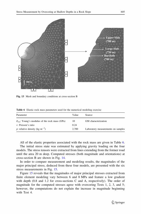
All of the elastic properties associated with the rock mass are given in Table 6.
The initial stress state was estimated by applying gravity loading on the four
models. The stress tensors were extracted from lines extending from the former road
until the area 20 m deep. Computed stresses (both magnitude and orientations) at
cross-section B are shown in Fig. 14.
In order to compare measurement and modeling results, the magnitudes of the
major principal stress, deduced from these four models, are presented with the six
stress measurements in Fig. 15.
Figure 15 reveals that the magnitudes of major principal stresses extracted from
finite element modeling vary between 6 and 8 MPa and feature a low gradient
with depth (0.8 and 1.2 for cross-sections C and A, respectively). The order of
magnitude for the computed stresses agree with overcoring Tests 1, 2, 3, and 5;
however, the computations do not explain the increase in magnitude beginning
with Test 4.
Fig. 13 Mesh and boundary conditions at cross-section B
Table 6 Elastic rock mass parameters used for the numerical modeling exercise
Parameter Value Source
Erm: Young’s modulus of the rock mass (GPa) 10 GSI characterization
v: Poisson’s ratio 0.24
p: relative density (kg m-3) 2,700 Laboratory measurements on samples
Stress Measurement by Overcoring at Shallow Depths in a Rock Slope 605
123

Furthermore, orientations of the major and minor stresses, as computed by the
2D finite element model (Fig. 14), show a significant topographic effect. For the
first 2 m, the major stress plunge is aligned with the local vertical free surface
(plunge: 90�), while the minor stress is horizontal. This first area corresponds
with the first overcoring test. On the other hand, from a depth of 2 m and
extending deeper, the computed major stresses tend to align with the mean dip
of the ‘‘large slab’’ (50–70�) until reaching a greater depth (around 300 m),
where the major stresses become vertical. The measured stresses show a more
scattered orientation, and the major stress plunge becomes vertical during Test 6
(18 m deep).
Numerical tests have, nonetheless, highlighted that the entire slope weight leads
to high stress magnitudes at the foot of the slope, a finding that complies with stress
measurements, even though anisotropy has not been taken into account in the
modeling set-up. However, the fact that stress magnitudes increase with depth, as
Fig. 14 Magnitudes and orientations of computed major principal stresses on cross-section B
Fig. 15 Measurements and modeling results for the major principal stress profile. The continuous linesrepresent numerical computations of major principal stresses for cross-sections A, B, C, and D.Overcoring Tests 1 through 6 are depicted using box plot squares (over the lower quartile Q1 = 25% andupper quartile Q3 = 75% of the data). The curves cross the median value points
606 C. Clement et al.
123

well as with orientation, has not been fully understood by this 2D computation. This
particular stress profile is obviously influenced by 3D topography, stress history, the
discontinuity network, and network heterogeneities. Further calculations, such as
those associated with 3D modeling, are foreseen.
6 Conclusion: Contributions Foreseen by this Study
Within the framework of multidisciplinary investigations at the Rochers deValabres rock slope site, the shallow stress field has been determined experimen-
tally at the foot of the slope composed of anisotropic gneiss.
Stress computations were performed using an experimental device and Monte
Carlo simulations. This process enabled us to highlight confidence intervals on the
stress module and orientation, in correlation with input data uncertainties. For the
studied case, the influence of anisotropy proved to be particularly acute, even
though the undulating foliation and mechanical dispersion remain significant.
Knowing the dispersion of these input data, the average standard deviations on
stress magnitude range between ±0.5 and ±0.9 MPa, which corresponds to 15–25%
of the stress quantity. This order of magnitude must be kept in mind for further
comparison with numerical modeling exercises or for all other conclusions drawn
from these stress measurements.
Moreover, these unusual stress measurements have provided us with information
on the stress field within the subsurface slope area. The measurements undertaken
have revealed that:
• The magnitudes of principal stresses are high, which complies with the simple
2D computation. Both computed and measured stresses have the same order of
magnitude, which corresponds to the overburden weight of the entire slope,
including the mountain crest.
• The subsurface area is heterogeneous and characterized by a high turnover of
the principal orientations and magnitude scattering. The initial measurements,
taken close to the surface and down to a depth of 7 m, are heavily influenced
by topography. Yet, topography is not the sole influential factor, as stress
history, the discontinuity network, and network heterogeneities have all been
hypothesized to explain stress heterogeneities, which indicates that a sizable
share of stress remains unpredictable and inaccessible due to a lack of
knowledge.
In conclusion, the stress measurements carried out as field experiments, through
the use of the overcoring test, have proven the feasibility of the overcoring
technique under rock slope conditions. Nevertheless, the results may not be
transposed to reach general assessments, as these investigations are characteristic of
the given site and depend on the particular stress determination techniques.
Acknowledgments This work program has been performed thanks to the financial support provided by
the French Ministry of Ecology and Sustainable Development. All authorizations and assistance from the
Mercantour National Park and the national EDF electric utility are gratefully acknowledged.
Stress Measurement by Overcoring at Shallow Depths in a Rock Slope 607
123

References
Akhpatelov DM, Ter-Martirosyan ZG (1971) The stressed state of ponderable semi-infinite domains.
Armenian Acad Sci Mech Bull 24:33–40
Amadei B (1983) Rock anisotropy and the theory of stress measurements. In: Brebbia CA, Orszag SA
(eds) Lecture Notes in Engineering. Springer, Heidelberg
Amadei B (1996) Importance of anisotropy when estimating and measuring in situ stresses in rock. Int J
Rock Mech Min Sci Geomech Abstr 33:293–325
Amadei B, Stephansson O (1997) Rock stress and its measurements. Chapman and Hall, London, pp 14,
45, 51, 96, 108–109
Ask D (2006) Measurement-related uncertainties in overcoring data at the Aspo HRL, Sweden. Part 2:
biaxial tests of CSIRO HI overcore samples. Int J Rock Mech Min Sci 43:127–138
Bertrand L (2001) Les mesures de contraintes in situ. La mesure et sa representativite en sciences de la
terre. Geologues 129:41–47
Bozzano F, Martino S, Priori M (2006) Natural and man-induced stress evolution of slopes: the Monte
Mario hill in Rome. Environ Geol 50:505–524
Clement C, Gunzburger Y, Merrien-Soukatchoff V, Dunner C (2008) Monitoring of natural thermal
strains using hollow cylinder strain cells: the case of a large rock slope prone to rockfalls. In:
Proceedings of the 10th International Symposium on Landslides and Engineered Slopes, Xi’an,
China, 30 June to 4 July 2008 (published)
Comite Francais de Mecanique des Roches (CFMR) (2004) Manuel de mecanique des roches, Tome 2:
les applications. Les Presses de l’Ecole des Mines, Paris, France. ISBN 2-911762-45-2, p 350
Cooling CM, Hudson JA, Tunbridge LW (1988) In situ rock stresses and their measurement in the U.K.—
Part II. Site experiments and stress field interpretation. Int J Rock Mech Min Sci Geomech Abstr
25:371–382
Cornet FH, Valette B (1984) In situ stress determination from hydraulic injection test data. J Geophys Res
89:11527–11537
Demin AM, Gorbacheva NP, Rulev AB (2003) Pattern of normal tension cracks on the landing of open pit
bench as an energy characteristic of landslide. J Min Sci 39(6):552–555
Dunner C, Bigarre P, Clement C, Merrien-Soukatchoff V, Gunzburger Y (2007) Field natural and thermal
stress measurements at ‘‘Rochers de Valabres’’ Pilot Site Laboratory. In: Proceedings of the 11th
Congress of the International Society for Rock Mechanics (ISRM), Lisbon, Portugal, 9–13 July 2007
Glamheden R, Curtis P (2006) Excavation of a cavern for high-pressure storage of natural gas. Tunn
Undergr Space Technol 21:56–67
Goodman RE (1980) Introduction to rock mechanics. Wiley, New York, pp 104–105
Gunzburger Y (2004) Role de la thermique dans la predisposition, la preparation et le declenchement des
mouvements de versants complexes. Exemple des Rochers de Valabres (Alpes-Maritimes). PhD
Thesis, LAEGO, Ecole des Mines, INPL, France, 174 pp
Gunzburger Y, Merrien-Soukatchoff V, Guglielmi Y (2005) Influence of daily surface temperature
fluctuations on rock slope stability: case study of the Rochers de Valabres slope (France). Int J Rock
Mech Min Sci 42:331–349
Haimson BC (1979) New hydro-fracturing measurements in the Sierra Nevada mountains and the
relationship between shallow stresses and surface topography. In: Proceedings of the 20th US
Symposium on Rock Mechanics, Center for Earth Sciences and Engineering, Austin, Texas, June
1979, pp 675–82
Heusermann S, Eickemeier R, Sprado K-H, Hoppe F-J (2003) Initial rock stress in the Gorleben salt dome
measured during shaft sinking. In: Proceedings of the GTMM International Symposium on
Geotechnical Measurements and Modelling, Karlsruhe, Germany, 23–26 September 2003
Hoek E (2006) Practical Rock Engineering. Available on http://www.rocscience.com/hoek/
PracticalRockEngineering.asp.
Hoek E, Brown ET (1988) The Hoek–Brown failure criterion—a 1988 update. In: Rock Engineering for
Underground Excavations, Proceedings of the 15th Canadian Rock Mechanics Symposium,
Toronto, Canada, pp 31–38
Hoek E, Brown ET (1997) Practical estimates of rock mass strength. Int J Rock Mech Min Sci Geomech
Abstr 34:1165–1186
Hoek E, Diederichs M (2006) Empirical estimation of rock mass modulus. Int J Rock Mech Min Sci
43:203–215
608 C. Clement et al.
123

Hooker VE, Johnson CF (1969) Near surface horizontal stresses including the effects of rock anisotropy.
US Bureau of Mines Report of Investigations RI 7224
Kang SS, Jang BA, Kang CW, Obrara Y, Kim JM (2002) Rock stress measurements and the state of stress
at an open-pit limestone mine in Japan. Eng Geol 67:201–217
Lahaie F (2005) Impact de l’anisotropie des proprietes elastiques sur l’estimation des contraintes in situ
par surcarottage. INERIS technical report DRS-05-56162/RN03
Lahaie F, Renaud V (2005) Optimisation de la procedure d’analyse et d’interpretation des donnees de
sous-carottage. INERIS technical report DRS-05-61593/RN01
Lahaie F, Bigarre P, Al Heib M, Josien JP, Noirel JF (2003) Large-scale 3D characterization of in-situ
stress field in a complex mining district prone to rockbursting. In: Proceedings of the 10th
International Congress on Rock Mechanics (ISRM), Sandton City, South Africa, 8–12 September
2003, pp 689–694
Ling CB (1947) On the stresses in a notched plate under tension. J Math Phys 26:284–289
Merrien-Soukatchoff V, Clement C, Senfaute G, Gunzburger Y (2005) Monitoring of a potential rockfall
zone: the case of ‘‘Rochers de Valabres’’ site. In: International Conference on Landslide Risk
Management, Proceedings of the 18th Annual Vancouver Geotechnical Society Symposium,
Vancouver, Canada, 31 May to 3 June 3 2005. CD-ROM
Merrien-Soukatchoff V, Sausse J, Dunner D (2006) Influence of topographic roughness and surface
rheology on the stress state in a sloped rock-mass. In Proceedings of Eurock 2006: Multiphysics
Coupling and Long Term Behaviour in Rock Mechanics, Liege, Belgium, 9–12 May 2006
Merrien-Soukatchoff V, Clement C, Gunzburger Y, Dunner D (2007) Thermal effects on rock slopes:
case study of the ‘‘Rochers de Valabres’’ slope (France). In: ISRM 2007, Specialized Sessions on
Rockfall—Mechanism and Hazard Assessment, Lisbon, Portugal, 9–13 July 2007
Obara Y, Nakamura N, Kang SS, Kaneko K (2000) Measurement of local stress and estimation of
regional stress associated with stability assessment of an open-pit rock slope. Int J Rock Mech Min
Sci 37:1211–1221
Pan E, Amadei B (1994) Stresses in anisotropic rock mass with irregular topography. ASCE J Eng Mech
120:97–119
Panthi KK, Nilsen B (2006) Numerical analysis of stresses and displacements for the Tafjord slide,
Norway. Bull Eng Geol Env 65:57–63
Savage WZ, Swolfs HS, Powers PS (1985) Gravitational stresses in long symmetric ridges and valleys.
Int J Rock Mech Min Sci Geomech Abstr 22:291–302
Senfaute G, Merrien-Soukatchoff V, Clement C, Laoufa F, Dunner C, Pfeifle G, Guglielmi Y, Lancon H,
Mudry J, Darve F, Donze F, Duriez J, Pouya A, Bemani P, Gasc M, Wassermann J (2006) Impact of
climate change on rock slope stability: monitoring and modelling. In: Proceedings of the
International Conference on Landslides and Climate Change, Ventnor, Isle of Wight, UK, 21–24
May 2007
Stephansson O (1993) Rock stress in the Fennoscandian shield. In: Hudson JA (ed) Comprehensive rock
engineering. Pergamon Press, Oxford
Tukey JW (1977) Exploratory data analysis. Addison-Wesley, Reading, MA. ISBN 0-201-07616-0
Walter JR, Martin CD, Dzik EJ (1990) Confidence intervals for in situ stress measurements. Technical
note. Int J Rock Mech Min Sci 27:139–141
Worotnicki G (1993) CSIRO triaxial stress measurement cell. In: Hudson JA (ed) Comprehensive rock
engineering, vol 3. Pergamon Press, Oxford, pp 329–394
Stress Measurement by Overcoring at Shallow Depths in a Rock Slope 609
123


![PC0710 J-DRain · [DIMPLE DRAIN CORE / NON-WOVEN GEOTEXTILE] An excellent choice for light commercial and residential construction. Maintains a very high flow rate for shallow depths](https://img.pdfslide.us/doc/110x75/5eda9c4209f66a09130ba02d/pc0710-j-drain-dimple-drain-core-non-woven-geotextile-an-excellent-choice-for.jpg)