Embed Size (px)
Citation preview
Kasetsart J. (Nat. Sci.) 47 : 143 - 154 (2013)
Civil Engineering Program, Sirindhorn International Institute of Technology, Thammasat University, Pathum Thani 12121, Thailand.* E-mail: [email protected]
Received date : 17/10/12 Accepted date : 25/12/12
Verification and Modification of Conversion Formulas for Estimating Statistical-Based Representative Wave Heights from
Zeroth Moment of Wave Spectrum Based on Field Data
Winyu Rattanapitikon
ABSTRACT
Conversion formulas were studied for estimating statistical-based representative wave heights (the mean wave height (Hm), root-mean-square wave height (Hrms ), average of the highest one-third wave height (H1/3) and average of the highest one-tenth wave height (H1/10)) from the zeroth moment of the wave spectrum (m0). The applicability of five sets of existing conversion formulas was examined based on two field experiments of the COAST3D project (using 13,430 wave records). The examination showed that the conversion formulas derived from the Weibull distribution with a constant shape parameter gave the best prediction. The best set of conversion formulas was modified by reformulating the shape parameter in the formulas. The modified formulas gave slightly better predictions at Hm , Hrms and H1/3 , and considerably better prediction at H1/10 than those of existing formulas. The modified formulas can be applied from shallow water to deepwater.Keywords: wave height distribution, representative wave height, zeroth moment of wave spectrum,
conversion formula
INTRODUCTION
Representative wave height is one of the most essential required factors for many coastal and ocean engineering applications such as the design of structures and the study of beach deformations. There are two basic approaches to describing wave height parameters, —the statistical approach (or wave-by-wave approach) and the spectral approach. The two approaches are both important, and neither one alone is sufficient for the successful application of wave height analysis in engineering problems (Goda, 1974). While some formulas in coastal and ocean engineering are appropriate for statistical-based
wave heights, others may be more appropriate for spectral-based wave heights that are related to the zeroth moment of wave spectrum (m0). The statistical-based wave heights should be used in those applications where the effect of individual waves is more important than the average wave energy. Measured ocean wave records are often analyzed spectrally by an instrument package. Similarly, modern wave hindcasts are often expressed in terms of spectral-based wave height (or m0). The spectral-based wave heights are usually available in deepwater, but not available at the depths required in shallow water. The wave heights in shallow water can be determined from a spectral-based wave model. Hence the output of
Kasetsart J. (Nat. Sci.) 47(1)144
the wave model is the spectral-based wave height, for example, the spectral significant wave height ( H mm0 04= ). However, some formulas in coastal and ocean engineering applications are expressed in terms of statistical-based representative wave heights. Therefore, it is necessary to know conversion formulas for converting from m0 to statistical-based representative wave heights. The present study focused on conversion formulas for converting from common parameters obtained from the spectral-based wave model—that is , m0 , water depth (h) and the spectral peak period (Tp)—to the four common statistical-based representative wave heights—namely, the mean wave height (Hm), root-mean-square wave height (Hrms), average of the highest one-third wave height (H1/3) and average of the highest one-tenth wave height (H1/10). Conversions formulas are usually derived based on a given probability distribution function of wave heights. Longuet-Higgins (1952) first applied a Rayleigh distribution function to describe the distribution of ocean waves under the conditions of a narrow band spectrum and linear Gaussian ocean surface. If the Rayleigh distribution of wave heights is valid, the representative wave heights can be determined from m0 through known proportional constants, for example, H m1 3 04/ = . Because of their simplicity, the conversion formulas of Longuet-Higgins (1952) are widely used in practical work. However, based on the analysis of field data for wind-driven waves in deepwater, Goda (1979) found that the proportional constants have to be reduced, for example, H m1 3 03 8/ .≈ . This discrepancy was considered to be caused by the broad band spectrum in the field (Longuet-Higgins, 1980). Moreover, when waves propagate in shallow water, the effect of wave breaking may become relevant, causing the wave height distribution to deviate from the Rayleigh distribution. Nevertheless, it is not clear whether this deviation has a significant effect on the estimation of the representative wave heights or not. Some researchers demonstrated
that the wave height distribution deviated slightly from the Rayleigh distribution (Goda and Kudaka, 2007; Risio et al., 2010). On the other hand, several researchers stated that the wave height distribution deviated considerably from the Rayleigh distribution (Klopman, 1996; Battjes and Groenendijk, 2000). Several conversion formulas with depth-limited wave breaking have been proposed for computing the representative wave heights in shallow water. Battjes and Groenendijk, (2000) compared the accuracy of their formulas with those of Longuet-Higgins (1952) and Klopman (1996), and found that their formulas gave the best prediction for small-scale laboratory data. The main difference between laboratory and field experiments is the incident wave spectrum. In the laboratory, the incident wave spectrum is usually based on some standard spectra (for example, the so-called TMA and JONSWAP spectra), while the actual wave spectra in the field usually exhibit some deviations from the standard spectra (Goda, 2000). Therefore, it is not clear, whether the formulas developed based on laboratory conditions are applicable in the field or not. The main objective of this study was to examine five sets of existing conversion formulas with field experiments, and to develop a suitable set of conversion formulas.
EXISTING FORMULAS
For the statistical approach, an individual wave in a wave record is determined by a zero crossing definition of the wave. A wave is defined between two upward (or downward) crossings of the water surface about the mean water elevation. The wave height (H) of an individual wave is defined as the difference between the highest and lowest water surface elevation between two zero-up-crossings (or zero-down-crossings). The statistical-based representative wave heights (Hm , Hrms , H1/3 and H1/10) can be determined from the wave heights data of the wave record.
Kasetsart J. (Nat. Sci.) 47(1) 145
For the spectral approach, the moments of a wave spectrum are important in characterizing the spectrum and are useful in relating the spectral description of the wave to the statistical-based wave heights. The representative parameter of the average wave energy is the zeroth moment of the wave spectrum (m0 ), which can be obtained by integrating the wave spectrum, S(f), in the full range of frequency, f, as shown in Equation 1:
m S f df00
=∞( )∫ (1)
Conversion formulas for computing the statistical-based representative wave heights from the known m0 can be derived from a given probability density function (pdf) of wave heights. Various pdfs of wave heights have been proposed; some of them are expressed in terms of uncommon output parameters, which are not available from some existing spectral-based wave models (for example, spectral bandwidth, spectral shape and wave nonlinearity parameters), such as the distributions of Tayfun and Fedele (2007), Vandever et al. (2008) and Petrova and Soares (2011). Including more related parameters is expected to make the pdf more accurate. However, it may not be suitable to incorporate them with some spectral-based wave models because such parameters are not available from the wave models. Therefore, this study concentrated on only pdfs which are expressed in terms of common parameters obtained from the spectral-based wave model, that is m0 , h and Tp. Brief reviews of the selected existing conversion formulas are described below. a) Longuet-Higgins (1952), hereafter referred to as LH52, demonstrated that a Rayleigh distribution is applicable to the wave heights in the sea. The Rayleigh distribution is derived based on the assumption that ocean surface elevations follow a linear Gaussian distribution and the wave energy is concentrated in a narrow band of frequencies. The cumulative distribution function (cdf) of Rayleigh is expressed using Equation 2:
F H H
m( ) exp= − −
18 0
2
(2)
where H is the individual wave height, and F(H) is the cdf of H. Longuet-Higgins (1952) derived the conversion formulas based on this cdf. The root-mean-square wave height can be calculated from the second moment of the pdf by Equation 3:
( )20 0
0
2( 1) 8 82rmsH H f H dH m m
∞= = Γ + =∫
(3)
where f(H) = dF(H)/dH is the pdf of H and Γ(x) is the Gamma function of variable x. The formula for computing the average of the highest 1/N wave heights is obtained by manipulation of the pdf of wave heights. The result is shown in Equation 4: 0/1
1( ) 1, ln 82N
NH
H N Hf H dH N N m∞
= = Γ +∫
(4)
where H1/N is the average of the highest 1/N wave heights, N is the number of individual waves, HN
is the wave height with exceedance probability of 1/N and Γ(a, x) is the upper incomplete Gamma function of variables a and x. The representative wave heights (Hm , H1/3 and H1/10) can be determined by substituting N equal to 1, 3 and 10, respectively, into Equation 4. b) Forristall (1978), hereafter referred to as F78, analyzed deepwater wave data recorded during hurricanes in the Gulf of Mexico and suggested that wave height distribution fits well with the Weibull distribution described by Equation 5:
F H H
m( ) exp
.
.
= − −
12 724 0
2 126
(5)
Following the same procedures as that of LH52, the formulas for computing Hrms and H1/N can be derived using Equations 6 and 7, respectively:
Kasetsart J. (Nat. Sci.) 47(1)146
H m mrms = + =2 724 2
2 1261 2 6892
0 0. (.
) . (6)
H NN1 02 724 12 126
1/ ..
, ln( )
+= Nm (7)
From the known m0 , the root-mean-square wave height (Hrms) is determined from Equation 6 and the other representative wave heights (H1/N) are determined from Equation 7. c) Klopman (1996), hereafter referred to as K96, used the same probability function as that of Glukhovskiy (1966). He modified the distribution of Glukhovskiy (1966) by reformulating the position and shape parameters. The relationship between Hrms and m0 was assumed to be the same as that of LH52 (Equation 3). The Weibull distribution, described by Equation 8, is used to describe the wave height distribution:
F H A H
m( ) exp= − −
18 0
κ
(8)
where A is the position parameter and κ is the shape parameter. The influence of depth-limited wave breaking is taken into account by including a function of Hrms/h (or m h0 / ) into the shape parameter as shown in Equation 9:
−2
1 1 98 0. /m h= (9)
where h is the water depth. To assure consistency, the second moment of the pdf has to be equal to Hrms
2 . This yields the position parameter (A) as Equation 10: A = +
Γ
2 12
κ
κ /
(10)
Similar to the derivation of LH52, the formula for computing the average of the highest 1/N wave heights (H1/N) is obtained by manipulation of the pdf of wave heights. The formula for computing H1/N can be derived as Equation 11:
H N Hf∫ H dH N
AN mN
HN1 1 0
1 1 8/ /( ) , ln= = +
∞
κ κΓ
(11)From the known m0 and h , the root-mean-square wave height (Hrms) is determined from Equation 3 and the other representative wave heights (H1/N) are determined from Equation 11, in which the parameters κ and A are determined from Equations 9 and 10, respectively. It should be noted that the Rayleigh distribution is considered as a special case of the Weibull distribution. If the parameter κ is equal to 2, the formulas of K96 will become the same as those of LH52. d) Battjes and Groenendijk (2000), hereafter referred to as BG00, proposed a composite Weibull wave height distribution to describe the wave height distribution on a shallow foreshore. The distribution consists of a Weibull distribution with an exponent of 2.0 for the lower wave heights and a Weibull distribution with an exponent of 3.6 for the higher wave heights. The two Weibull distributions are matched at the transitional wave height (Htr). The pdf is expressed by Equation 12:
2H H
F H
HH
H H
HH
tr
( )
exp
exp.
=
− −
− −
<1
1
1
2
3 6
for
≥for tr
(12)
where H1 and H2 are the scale parameters. The transitional wave height (Htr) is determined from the empirical formula of Equation 13:
Htr = (0.35 + 5.8m)h (13)
where m is the beach slope. For convenience in the calculations, all wave heights are normalized with Hrms using Equation 14: H
HHx
x
rms= (14)
Kasetsart J. (Nat. Sci.) 47(1) 147
where H x is the normalized characteristic wave height. The root-mean-square wave height (Hrms) is proposed as a function of m0 and h as shown in Equation 15: H
mh
mrms = +2 69 3 24 00. . (15)
The normalized scale parameters H1 and H2 are determined by solving Equations 16 and 17 simultaneously: � � �
�H H HHtrtr
21
2/3.6
= (16) 1 2 1 5561
2
1
2
22
2
3
= +� ��
� ��H
HH
HHH
tr trγ , . ,.
Γ66
(17)where g(a, x) is the lower incomplete Gamma function of variables a and x. After manipulation of the probability function (more detail is provided in Groenendijk, 1998), the normalized HN and H1/N are expressed using Equations 18 and 19:
�� � �
� � �H
HH
H N H H
H N H HN
N
rms
N tr
N tr
= =[ ] <
[ ] ≥
11 2
21 3 6
ln
ln
/
/ .
for
for
(18)
HH
NH NHHN
rms
tr1 1
1
2
1 5 1 5/ . , ln . ,=
[ ]−
� ��à à + <NH
HH
H H
NH
trN tr
� ��
� �
�
22
3 6
2
1.278,
1 27
Γ
Γ .
.
for
88, ln N H HN tr[ ] ≥for � �
HH
NH NHHN
rms
tr1 1
1
2
1 5 1 5/ . , ln . ,=
[ ]−
� ��à à + <NH
HH
H H
NH
trN tr
� ��
� �
�
22
3 6
2
1.278,
1 27
Γ
Γ .
.
for
88, ln N H HN tr[ ] ≥for � �
(19)
From the known m0 , h and m , the root-mean-square wave height (Hrms) is determined from Equation 15 and the normalized scale parameters H1 and H2 are determined from Equations 16
and 17 simultaneously. Once H1 and H2 have been determined, H1/N can be determined from Equations 18 and 19.
e) Elfrink et al. (2006), hereafter referred to as EHR06, used the same probability function as that of K96 and, consequently, the same conversion formulas for computing Hrms and H1/N by Equations 3 and 11, respectively. They modified the distribution of K96 by reformulating the shape parameter (κ). The proposed formula for computing the parameter κ of EHR06 is expressed by Equation 20: κ −
+= 15.5 2.03
2 2
tanhHh
Hh
rms rms (20)
From the known m0 and h , the representative wave heights Hrms and H1/N are determined from Equations 3 and 11, respectively, in which the parameters κ and A are determined from Equations 20 and 10, respectively.
COLLECTED EXPERIMENTAL DATA
The existing models of wave height distribution (or conversion formulas) are determined by the local parameters of wave field and water depth. The models are expected to be valid for the slow evolution of a wave and bathymetry (Battjes and Groenendijk, 2000) and to be influenced in a small manner by any discharge from a river or by wave reflection from structures. Therefore, the selected measuring stations should not be located close to structures or a river mouth or where there is a substantial change in the waves and bathymetry. The data required for examination of the conversion formulas are m0, h , Tp , Hm, Hrms , H1/3 and H1/10. Two field experiments to examine the conversion formulas (including 2,237 cases and 13,430 wave records) were used from the COAST3D project, a collaborative project co-funded by the European Commission’s MAST-III program and national resources (Soulsby, 1998). The experiments covered a range of m h0 / from 0.003 to 0.286 and a range of relative depth (h/L, where L is the wavelength) from 0.01 to 0.63. The collected wave data belong to the categories
Kasetsart J. (Nat. Sci.) 47(1)148
of deepwater, intermediate-depth and shallow water waves. A summary of the experimental data is shown in Table 1. A brief summary of the experiments is outlined below. The two field experiments were performed at two sites—Egmond-aan-Zee (Ruessink, 1999) and Teignmouth (Whitehouse and Sutherland, 2001). The Egmond site is located in the central part of the Dutch North Sea coast. The study area was about 0.5 by 0.5 km near the beach of Egmond. The site was dominated by two well-developed shore-parallel bars intersected by rip channels. Two field campaigns were executed—a pilot experiment (from April to May 1998) and main experiments (from October to November 1998). The experiments were divided into three conditions—pre-storm (pilot experiment), storm (main-A experiment) and post storm (main-B experiment). For the main-A experiment, large waves and water level rises due to storm surges were present, resulting in considerable bathymetric change (bar movement and the presence of rip channels). A large variety of instruments was deployed at many stations in the study area. The complete data at some stations was considered (stations 1a, 1b, 1c, 1d, 2, 7a, 7b, 7c, 7d and 7e for the pilot experiment; stations 1a, 1b, 1c, 1d, 2, 7a, 7b and 7e for the main-A experiment; and stations 1a, 1b, 1c, 1d, 2, 7b, 7d and 7e for the main-B experiment. Most available stations (except station 2 for the main-A experiment) were used in this study. Station 2 was located close to the crest of a sand bar. Because of the considerable changes to the waves and the sand bar during storms, the data from station 2 for the main-A experiment was excluded in the present study. The Teigmond site is located on the south coast of Devon, UK. The study area was about 1.5 km along the beach by 1.0 km offshore of the beach. The Teign river mount is situated at the southern end of the beach. The beach is protected by groins and seawalls. A leisure pier is
situated about mid-way along the beach. Two field campaigns were executed—a pilot experiment (in March 1999) and a main experiment (from October to November 1999). During the experiments, bathymetric changes were minor. A large variety of instruments was deployed at many stations in the study area. The data of water depth and representative wave heights were available at some stations (stations 1, 2, 15, 18, 22 and 25 for the pilot experiment and stations 1, 2, 3a, 4, 6, 9, 10, 15, 18, 19a, 20a, 25, 28, 29, 32 and 33 for the main experiment). If stations are located close to structures or the river mouth, the wave spectra may be affected by discharge from the river and wave reflection from the structures. Consequently, only data at stations which were not located close to structures or the river mouth were used in the present study—namely, stations 15, 18, 22 and 25 for the pilot experiment and stations 3a, 4, 6, 9, 10, 15, 18, 25, 28, 32 and 33 for the main experiment.
EXAMINATION OF EXISTING FORMULAS
The basic parameter for measuring the accuracy of the conversion formulas is the root-mean-square relative error (ER) as defined in Equation 21: ER
∑
∑
H H
H
cr i mr ii
n
mr ii
n=−
=
=
100
2
1
2
1
( ), ,
,
(21)
where Hcr is the computed representative wave height, Hmr is the measured representative wave height and n is the total number of representative wave heights. It is expected that a good set of formulas should be able to provide a good prediction for all representative wave heights. Therefore, the average error (ERavg) from the four representative wave heights was used to examine the overall accuracy of the set of formulas.
Kasetsart J. (Nat. Sci.) 47(1) 149
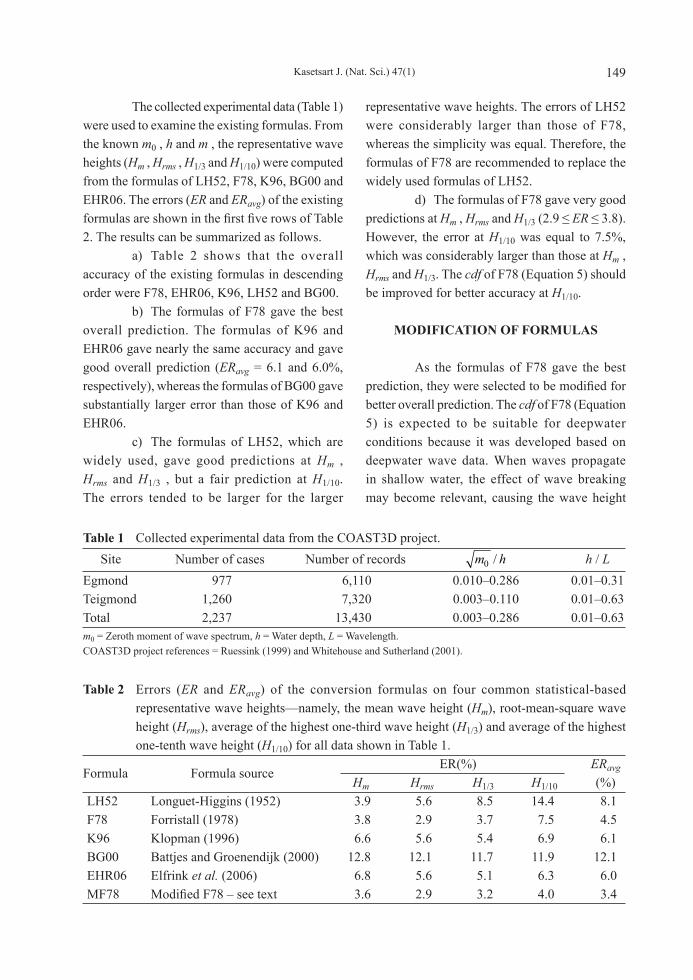
The collected experimental data (Table 1) were used to examine the existing formulas. From the known m0 , h and m , the representative wave heights (Hm , Hrms , H1/3 and H1/10) were computed from the formulas of LH52, F78, K96, BG00 and EHR06. The errors (ER and ERavg) of the existing formulas are shown in the first five rows of Table 2. The results can be summarized as follows. a) Table 2 shows that the overall accuracy of the existing formulas in descending order were F78, EHR06, K96, LH52 and BG00. b) The formulas of F78 gave the best overall prediction. The formulas of K96 and EHR06 gave nearly the same accuracy and gave good overall prediction (ERavg
= 6.1 and 6.0%, respectively), whereas the formulas of BG00 gave substantially larger error than those of K96 and EHR06. c) The formulas of LH52, which are widely used, gave good predictions at Hm , Hrms and H1/3 , but a fair prediction at H1/10. The errors tended to be larger for the larger
representative wave heights. The errors of LH52 were considerably larger than those of F78, whereas the simplicity was equal. Therefore, the formulas of F78 are recommended to replace the widely used formulas of LH52. d) The formulas of F78 gave very good predictions at Hm , Hrms and H1/3 (2.9 ≤ ER ≤ 3.8). However, the error at H1/10 was equal to 7.5%, which was considerably larger than those at Hm , Hrms and H1/3. The cdf of F78 (Equation 5) should be improved for better accuracy at H1/10.
MODIFICATION OF FORMULAS
As the formulas of F78 gave the best prediction, they were selected to be modified for better overall prediction. The cdf of F78 (Equation 5) is expected to be suitable for deepwater conditions because it was developed based on deepwater wave data. When waves propagate in shallow water, the effect of wave breaking may become relevant, causing the wave height
Table 1 Collected experimental data from the COAST3D project. Site Number of cases Number of records m h0 / h / LEgmond 977 6,110 0.010–0.286 0.01–0.31Teigmond 1,260 7,320 0.003–0.110 0.01–0.63Total 2,237 13,430 0.003–0.286 0.01–0.63m0 = Zeroth moment of wave spectrum, h = Water depth, L = Wavelength.COAST3D project references = Ruessink (1999) and Whitehouse and Sutherland (2001).
Table 2 Errors (ER and ERavg) of the conversion formulas on four common statistical-based representative wave heights—namely, the mean wave height (Hm), root-mean-square wave height (Hrms), average of the highest one-third wave height (H1/3) and average of the highest one-tenth wave height (H1/10) for all data shown in Table 1.
ER(%) ERavg
Hm Hrms H1/3 H1/10 (%)LH52 Longuet-Higgins (1952) 3.9 5.6 8.5 14.4 8.1F78 Forristall (1978) 3.8 2.9 3.7 7.5 4.5K96 Klopman (1996) 6.6 5.6 5.4 6.9 6.1BG00 Battjes and Groenendijk (2000) 12.8 12.1 11.7 11.9 12.1EHR06 Elfrink et al. (2006) 6.8 5.6 5.1 6.3 6.0MF78 Modified F78 – see text 3.6 2.9 3.2 4.0 3.4
Formula Formula source
Kasetsart J. (Nat. Sci.) 47(1)150
distribution to deviate from that of F78. Following the concept of Klopman (1996), the effect of depth-limited breaking is taken into account by including a function of m h0 / in the shape parameter of the cdf. The cdf of F78 can be written in general form using Equation 22:
F H P H
C m
S
( ) exp= − −
11 0
(22)
in which Equations 22 and 23 describe: H C mrms = 1 0 (23) S fu
mh
n= 0
(24)
where P is the position parameter, S is the shape parameter, C1 is constant and fu xn { } is a function of variable x. If S = 2.126, C1 = 2.689 and P = 0.973, Equation 22 will become the distribution of F78 (Equation 5).
From H H f H dH∫rms = ( )∞
2
0, the posit ion
parameter ( P ) can be expressed by Equation 25: P
S
S
= +
Γ2 1
2/
(25)
The average of the highest 1/N wave heights (H1/N) is determined from Equation 26: H N Hf H dH N
P SN C mN
HS
N1 1 1 0
1 1/ /( ) , ln= = +
∞
Γ∫
H N Hf H dH NP S
N C mNH
SN
1 1 1 01 1/ /( ) , ln= = +
∞
Γ∫ (26)
It can be seen that there are two independent parameters in Equation 22, namely, C1 and S. The main objective of this section is to determine the value of C1 and the formula of S.
Determination of C1 and S As the experiment at Egmond covered
a wide range of m h0 / , it was used to calibrate and formulate C1 and S. The constant C1 can be determined from regression analysis between measured Hrms and m0 . The required data for determining C1 are the measured data of Hrms and m0. Based on a regression analysis between the measured Hrms and m0 , the constant C1 is equal to 2.69 (with regression coefficient R2 = 0.995). Substituting C1 = 2.69 into Equation 23, the formula for computing Hrms can be expressed as Equation 27: H mrms = 2 69 0. (27)
It can be seen that the value of C1 is the same as that of F78. This means that the value of C1 in F78 is already the optimal value. The formula of the shape parameter (S) is determined from the graph which shows the relationship between measured S and m h0 / . The data of m0 and h are available from the measurements. The measured value of S can be determined from the measured data of the wave height distribution or by the representative wave heights of a wave record. In the present study, the measured S was determined from the measured representative wave heights because the measured wave height distribution was not available. The measured S can be determined from the ratio of representative wave heights as follows. From Equation 26, the rat io of representative wave heights (H1/10/Hm , H1/10/H1/3 and H1/3/Hm) can be expressed as Equations 28, 29 and 30, respectively: HH
S
Sm
1 1010 1 1 10
1 1 1
/, ln
, ln=
+
+
Γ
Γ (28)
HH
S
S
1 10
1 3
10 1 1 10
3 1 1 3
/
/
, ln
, ln=
+
+
Γ
Γ
(29)
Kasetsart J. (Nat. Sci.) 47(1) 151
HH
S
Sm
1 33 1 1 3
1 1 1
/, ln
, ln=
+
+
Γ
Γ
(30)
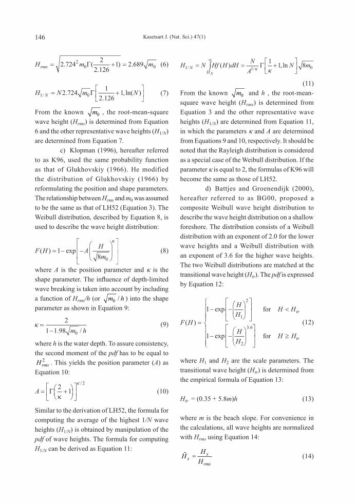
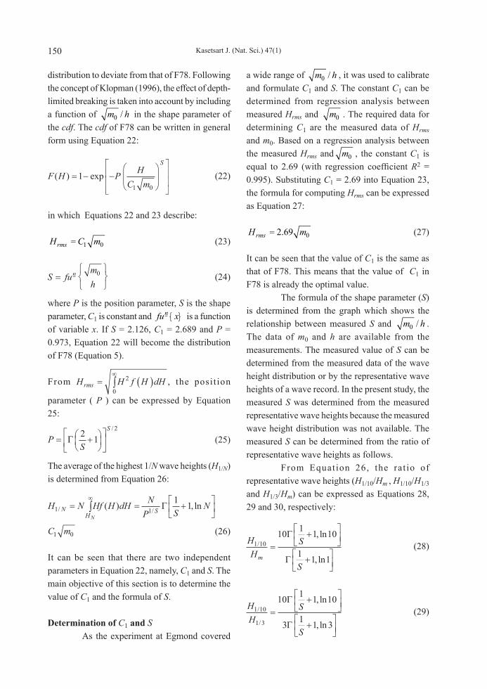
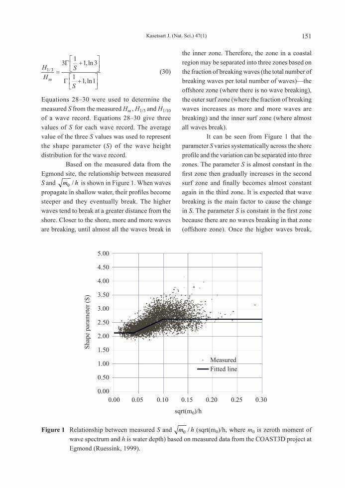
Equations 28–30 were used to determine the measured S from the measured Hm , H1/3 and H1/10 of a wave record. Equations 28–30 give three values of S for each wave record. The average value of the three S values was used to represent the shape parameter (S) of the wave height distribution for the wave record. Based on the measured data from the Egmond site, the relationship between measured S and m h0 / is shown in Figure 1. When waves propagate in shallow water, their profiles become steeper and they eventually break. The higher waves tend to break at a greater distance from the shore. Closer to the shore, more and more waves are breaking, until almost all the waves break in
the inner zone. Therefore, the zone in a coastal region may be separated into three zones based on the fraction of breaking waves (the total number of breaking waves per total number of waves)—the offshore zone (where there is no wave breaking), the outer surf zone (where the fraction of breaking waves increases as more and more waves are breaking) and the inner surf zone (where almost all waves break). It can be seen from Figure 1 that the parameter S varies systematically across the shore profile and the variation can be separated into three zones. The parameter S is almost constant in the first zone then gradually increases in the second surf zone and finally becomes almost constant again in the third zone. It is expected that wave breaking is the main factor to cause the change in S. The parameter S is constant in the first zone because there are no waves breaking in that zone (offshore zone). Once the higher waves break,
Figure 1 Relationship between measured S and m h0 / (sqrt(m0)/h, where m0 is zeroth moment of wave spectrum and h is water depth) based on measured data from the COAST3D project at Egmond (Ruessink, 1999).
Shap
e pa
ram
eter
(S)
Fitted lineMeasured
sqrt(m0)/h
0.00 0.05 0.10 0.15 0.20 0.25 0.30
5.00
4.50
4.00
3.50
3.00
2.50
2.00
1.50
1.00
0.50
0.00
Kasetsart J. (Nat. Sci.) 47(1)152
the number of larger wave heights in a wave train is decreased due to wave breaking. This causes the pdf of the wave heights to be narrower (and causes S to become larger) than that in the offshore zone. As more and more waves are breaking, the parameter S is gradually increased in the second zone until almost all waves break, then, the parameter S becomes constant in the third zone. Hence the three zones in Figure 1 seem to correspond with the zones in the coastal region. To simplify the calculation, the general form of S was expressed using Equation 31:
S
K formh
x
KK Kx x
mh
x for xmh
x
K
=
≤
+−( )−( )
− < <
10
1
12 1
2 1
01 1
02
2 fformh
x02≥
(31)
where K1 , K2 , x1 and x2 are constants which can be determined from formula calibration. The approximated values of the constants K1 , K2 , x1 and x2 can be determined from a visual fit of Figure 1. These approximated values were used as the initial values in the calibration. Using the parameter S from Equation 31 with the given constants (K1 , K2 , x1 and x2) and C1 = 2.69, the representative wave heights (Hm , H1/3 and H1/10) can be determined from Equation 26. Then the errors ER and ERavg can be computed. The calibration of Equation 31 can be performed by gradually adjusting the constants K1 , K2 , x1 and x2 until the error (ERavg) becomes minimum. After calibration, the formula of S can be expressed by Equation 32:
S
formh
mh
= +−( )−( )
−
2.12 0.04
2 122 62 2 120 10 0 04
0 04
0
0.. .. .
. < <
≥
formh
formh
0.04 0.10
2.62 0.10
0
0
≤
(32)
The fitted line from Equation 32 is shown as the solid line in Figure 1. The modified formulas are hereafter referred to as MF78. However, it should be noted that the cdf models of LH52, K96 and EHR06 can also be written in the same general form as that of Equation 22. The modified formulas may also be considered as modifications of LH52, K96 and EHR06.
Examination of formulas All collected experimental data (Table 1) were used to examine the modified formulas (MF78). From the known m0 and h , the representative wave heights Hrms and H1/N were determined from Equations 27 and 26, respectively, in which the parameters S and P were determined from Equations 32 and 25, respectively. The errors (ER and ERavg) of MF78 on computing Hm , Hrms , H1/3 and H1/10 are shown in the sixth row of Table 2. The results are summarized as follows: a) The average errors of MF78 for computing Hm , Hrms , H1/3 and H1/10 were 3.6, 2.9, 3.2 and 4.0%, respectively. b) Compared with the formulas of F78, the accuracy of MF78 was improved slightly at Hm , Hrms and H1/3 , but improved substantially at H1/10. As C1 of F78 and MF78 was the same value, the main contribution of the improvement was the shape parameter S (Equation 32). c) tThe formulas of MF78 were more complex than those of F78, but the accuracy was better, especially at H1/10. It seems to be worthwhile to use MF78. As the shape parameter S from Eq. (32) yielded a better estimation than that of F78 (S = 2.126), it may be used to indicate the limitation of F78. Equation (32) reveals some limitations of F78 as follows: a) It can be seen from Equation 32 that the value of S in the offshore zone ( m h0 0 04/ .≤ ) is nearly the same as that of F78. This shows that the formulas of F78 should be valid for either deepwater or offshore zone conditions. This also
Kasetsart J. (Nat. Sci.) 47(1) 153
reveals that Equation 32 is limited for use in cases where the wave height distribution in deepwater (or in the offshore zone) is close to the distribution of F78 (Equation 5). b) In the surf zones ( m h0 0 04/ .> ), the number of larger wave heights in a wave train was decreased due to wave breaking. This caused the pdf of wave heights to be narrower (larger S) than that in the offshore zone. The shape parameter of F78 (S = 2.126) was smaller than that of MF78 (Equation 32). This means that the parameter S of F78 tended to be underestimated and, consequently, overestimated the number of large waves in the distribution. This seemed to be the cause of the considerable error at H1/10 of F78 (ER = 7.5%).
CONCLUSION
The present study was undertaken to determine suitable conversion formulas for estimating the statistical-based representative wave heights (Hm , Hrms , H1/3 and H1/10) from the common parameters obtained from the spectral-based wave model (m0 and h). Conversion formulas can be derived from a given cdf (or pdf ) of wave heights. Five existing cdf models were considered in this study—the models of LH52, F78, K96, BG00 and EHR06. Field data from the COAST3D project (including 13,430 wave records) were used to examine the accuracy of the existing conversion formulas on estimating the representative wave heights. The data covered the wave conditions from deepwater to shallow water. The examination showed that the formulas of LH52, F78, K96 and EHR06 each gave a good overall prediction, while the formulas of BG00 gave a fair overall prediction. Compared among the existing formulas, the formulas of F78 gave the best overall prediction. The formulas of F78 gave very good predictions at Hm , Hrms and H1/3 , but gave considerably larger error at H1/10. The cdf of F78 was modified by reformulating the formula of the shape parameter (S). The new shape
parameter revealed that the distribution of F78 was valid in the offshore zone, but overestimated the number of large waves in the surf zone. The modified formulas gave a better estimation than those of F78, especially for H1/10. The modified formulas are generalized and can compute the representative wave heights from shallow water to deepwater conditions.
LITERATURE CITED
Battjes, J.A. and H.W. Groenendijk. 2000. Wave height distributions on shallow foreshores. Coast. Eng. 40: 161–182.
Elfrink, B., D.M. Hanes and B.G. Ruessink. 2006. Parameterization and simulation of near bed orbital velocities under irregular waves in shallow water. Coast. Eng. 53: 915–927.
Forristall, G.Z. 1978. On the statistical distribution of wave heights in storm. J. Geophys. Res. 83: 2553–2558.
Glukhovskiy, B.Kh. 1966. Investigation of Sea Wind Waves. Leningrad, Gidrometeoizdat (reference obtained from Bouws, E. 1979. Spectra of extreme wave conditions in the Southern North Sea considering the influence of water depth. Proc. Sea Climatology Conference, Paris. pp. 51–71).
Goda, Y. 1974. Estimation of wave statistics from spectral information. Proc. Ocean Waves Measurement and Analysis Conference, ASCE: 320–337.
Goda, Y. 1979. A review on statistical interpretation of wave data. Report of Port and Harbour Research Institute 18: 5–32.
Goda, Y. 2000. Random Seas and the Design of Maritime Structures. World Scientific Publishing Co. Pte. Ltd. Singapore. 443 pp.
Goda, Y. and M. Kudaka. 2007. On the role of spectral width and shape parameters in control of individual wave height distribution. Coast. Eng. J. 49: 311–335.
Groenendijk, H.W. 1998. Shallow Foreshore Wave Height Statistics, MSc. Thesis. Department
Kasetsart J. (Nat. Sci.) 47(1)154
of Civil Engineering. Delft University of Technology. Delft, the Netherlands. 65 pp.
Klopman, G. 1996. Extreme Wave Heights in Shallow Water, Report H2486. WL/Delft Hydraulics. The Netherlands (reference obtained from Battjes, J.A. and H.W. Groenendijk. 2000. Wave height distributions on shallow foreshores. Coast. Eng. 40: 161–182).
Longuet-Higgins, M.S. 1952. On the statistical distribution of the heights of sea waves. J. Mar. Res. 11(3): 245–266.
Longuet-Higgins, M.S. 1980. On the distribution of the heights of sea waves: Some effects of nonlinearity and finite band width. J. Geophys. Res. 85: 1519–1523.
Petrova, P.G. and C.G. Soares. 2011. Wave height distributions in bimodal sea states from offshore basins. Ocean Eng. 38: 658–672.
Risio, M.D., I. Lisi, G.M. Beltrami and P.D. Girolamo. 2010. Physical modeling of the cross-shore short-term evolution of protected and unprotected beach nourishments. Ocean Eng. 37: 777–789.
Ruessink, B.G. 1999. COAST3D Data Report–2.5D Experiment, Egmond aan Zee, IMAU Report. Utrecht University. Utrecht, the Netherlands. 75 pp.
Soulsby, R.L. 1998. Coastal sediment transport: The COAST3D project. Proc. 26th Coastal Engineering Conference, ASCE: 2548–2558.
Tayfun, A. and F. Fedele. 2007. Wave height distribution and nonlinear effects. Ocean Eng. 34: 1631–1649.
Vandever, J.P., E.M. Siegel, J.M. Brubaker and C.T. Friedrichs. 2008. Influence of spectral width on wave height parameter estimates in coastal environments. J. Waterw. Port C. –ASCE 134(3): 187–194.
Whitehouse, R.J.S. and J. Sutherland. 2001. COAST3D Data Report–3D Experiment, Teignmouth, UK. HR Wallingford Report TR 119. 139 pp.