Embed Size (px)
Citation preview
Stress-Life and Crack Growth Calculations on an Aircraft Main Frame Section Using MSC.Fatigue
Neil Bishop, Marco Veltri and Andy Woodward
Date: 21 August 2001
Report Number: RLD010801
Please note that this work was supported by Alenia Aerospazio Divisione Aeronautica, Pomigliano D'Arco Napoli
RLD LtdEngineering Analysis And Design Hutton Roof, Eglinton Road, Tilford, Farnham, Surrey, GU10 2DH Tel 01252 792088 Fax 01252 794165 Registered Company Number 2953415
AEROSPAZIO Divisione Aeronautica

1
Stress-Life and Crack Growth Calculations on an Aircraft Main Frame Section Using MSC.Fatigue Neil Bishop, Marco Veltri and Andy Woodward, 21 August 2001
Summary The main objective of this project was to perform Stress-Life and crack growth calculations on a typical aircraft main frame section using MSC.Fatigue; Thereby demonstrating the possible usefulness of MSC.Fatigue as a general-purpose fatigue analysis tool. The project was based on a medium range passenger aircraft. This fatigue analysis software was used in conjunction with Nastran, Patran and Marc. The following tasks were undertaken.
• Set up model and check model quality (mesh density etc) • Perform Stress-Life fatigue analysis with MSC.Fatigue • Identify critical location • Investigate stress conditions in this region (MARC/Nastran) • Demonstrate current state-of-the-art techniques for dealing with fracture, stress
intensity function calculations and crack propagation analysis. • Perform crack growth calculation with MSC.Fatigue • Perform sensitivity studies related to load level
An Overview of FEA Based Fatigue Design
In fatigue design, three core fatigue methodologies have become established. The first two techniques that were developed do not model the crack growth process at all. Instead, they use the concept of similitude to determine the number of cycles to failure; ‘Failure’ being defined as some predetermined crack length, or loss of stiffness, or separation of the component being designed. This means that the relationship between component life and load level in a test specimen can be compared directly with that expected in service (assuming the component is tested under identical conditions). The first of these two methods is based on stress, the so-called Stress-Life (S-N, nominal stress, or total life) method. The second, and more recent technique is based on strain, the so-called Strain-Life (Local-Stress-Strain, Crack-Initiation, Manson-Coffin or Critical-Location Approach - CLA) method. The third, and most recently developed method deals with Crack-Propagation and relies on the observation that once cracks become established they have a stable growth period. This is usually described using linear elastic fracture mechanics. It further relies on the assumption that crack growth rates are proportional to the applied stress intensity (a function of crack length, geometry and stress level).
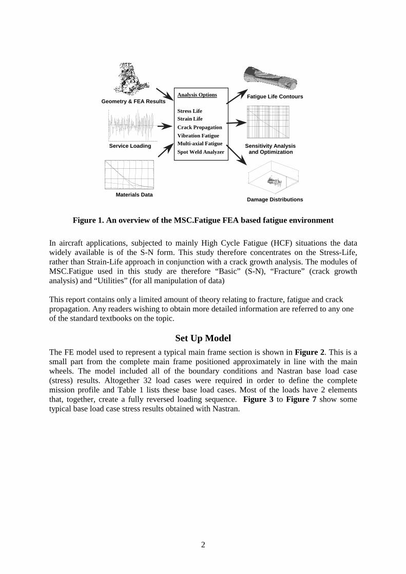
An Overview of the FEA Based Fatigue Environment MSC.Fatigue is the leading tool for FEA based fatigue design and Figure 1 gives an overview of the MSC.Fatigue FEA based fatigue environment. The three plots on the left indicate the FEA results, applied loading and materials information. The three plots on the right show the types of result visualisation that are possible. The centre box indicates the types of fatigue calculations that can be done. All of the fatigue techniques specified in Figure 1 are completely, or substantially, based on one of the three standard life estimation methods, i.e., Stress-Life, Strain-Life or Crack-Propagation, described in detail later.
2
Analysis Options
Stress LifeStrain LifeCrack PropagationVibration FatigueMulti-axial FatigueSpot Weld Analyzer
Geometry & FEA Results
Service Loading
Materials Data Damage Distributions
Fatigue Life Contours
Sensitivity Analysis and Optimization
Figure 1. An overview of the MSC.Fatigue FEA based fatigue environment In aircraft applications, subjected to mainly High Cycle Fatigue (HCF) situations the data widely available is of the S-N form. This study therefore concentrates on the Stress-Life, rather than Strain-Life approach in conjunction with a crack growth analysis. The modules of MSC.Fatigue used in this study are therefore “Basic” (S-N), “Fracture” (crack growth analysis) and “Utilities” (for all manipulation of data) This report contains only a limited amount of theory relating to fracture, fatigue and crack propagation. Any readers wishing to obtain more detailed information are referred to any one of the standard textbooks on the topic.
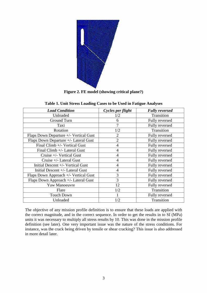
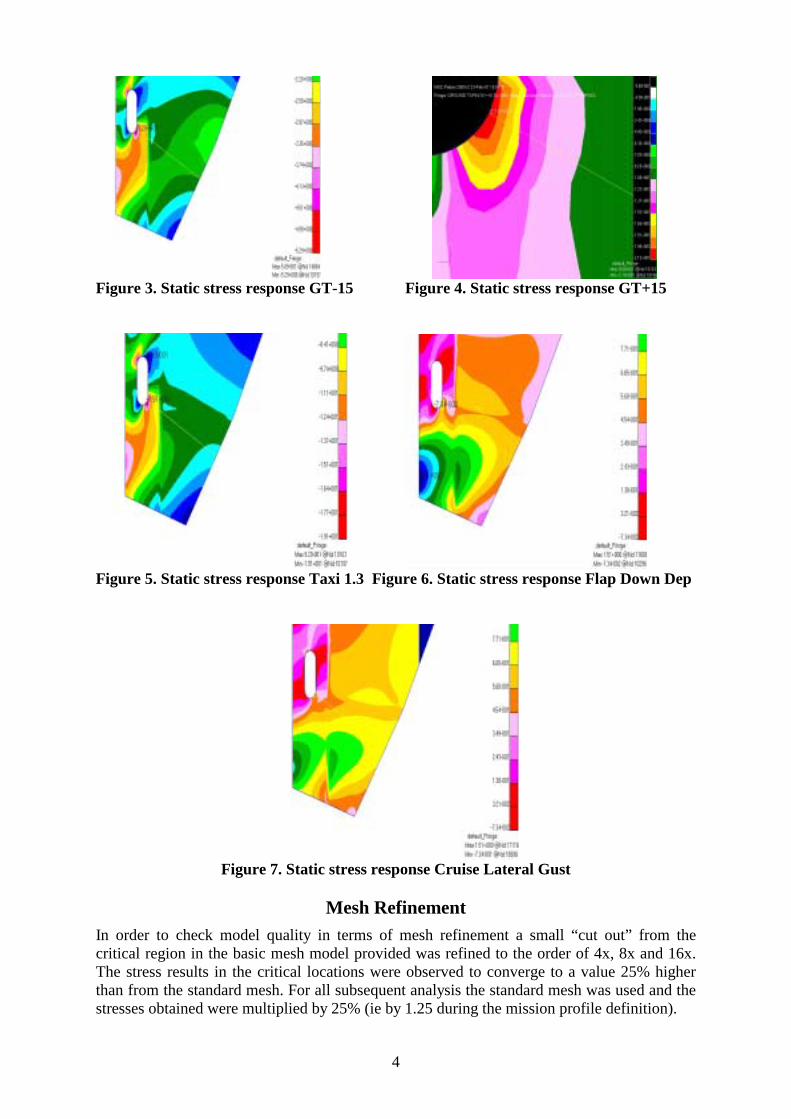
Set Up Model The FE model used to represent a typical main frame section is shown in Figure 2. This is a small part from the complete main frame positioned approximately in line with the main wheels. The model included all of the boundary conditions and Nastran base load case (stress) results. Altogether 32 load cases were required in order to define the complete mission profile and Table 1 lists these base load cases. Most of the loads have 2 elements that, together, create a fully reversed loading sequence. Figure 3 to Figure 7 show some typical base load case stress results obtained with Nastran.
3
Figure 2. FE model (showing critical plane?)
Table 1. Unit Stress Loading Cases to be Used in Fatigue Analyses
Load Condition Cycles per flight Fully reversed Unloaded 1/2 Transition
Ground Turn 6 Fully reversed Taxi 7 Fully reversed
Rotation 1/2 Transition Flaps Down Departure +/- Vertical Gust 2 Fully reversed Flaps Down Departure +/- Lateral Gust 2 Fully reversed
Final Climb +/- Vertical Gust 4 Fully reversed Final Climb +/- Lateral Gust 4 Fully reversed
Cruise +/- Vertical Gust 4 Fully reversed Cruise +/- Lateral Gust 4 Fully reversed
Initial Descent +/- Vertical Gust 4 Fully reversed Initial Descent +/- Lateral Gust 4 Fully reversed
Flaps Down Approach +/- Vertical Gust 3 Fully reversed Flaps Down Approach +/- Lateral Gust 3 Fully reversed
Yaw Manoeuvre 12 Fully reversed Flare 1/2 Transition
Touch Down 1 Fully reversed Unloaded 1/2 Transition
The objective of any mission profile definition is to ensure that these loads are applied with the correct magnitude, and in the correct sequence. In order to get the results in to SI (MPa) units it was necessary to multiply all stress results by 10. This was done in the mission profile definition (see later). One very important issue was the nature of the stress conditions. For instance, was the crack being driven by tensile or shear cracking? This issue is also addressed in more detail later.
4
Figure 3. Static stress response GT-15 Figure 4. Static stress response GT+15
Figure 5. Static stress response Taxi 1.3 Figure 6. Static stress response Flap Down Dep
Figure 7. Static stress response Cruise Lateral Gust
Mesh Refinement
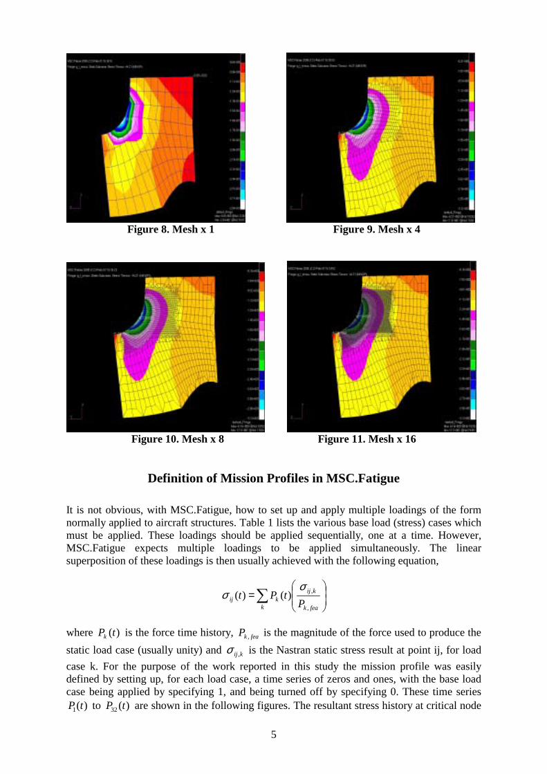
In order to check model quality in terms of mesh refinement a small “cut out” from the critical region in the basic mesh model provided was refined to the order of 4x, 8x and 16x. The stress results in the critical locations were observed to converge to a value 25% higher than from the standard mesh. For all subsequent analysis the standard mesh was used and the stresses obtained were multiplied by 25% (ie by 1.25 during the mission profile definition).
5
Figure 8. Mesh x 1 Figure 9. Mesh x 4
Figure 10. Mesh x 8 Figure 11. Mesh x 16
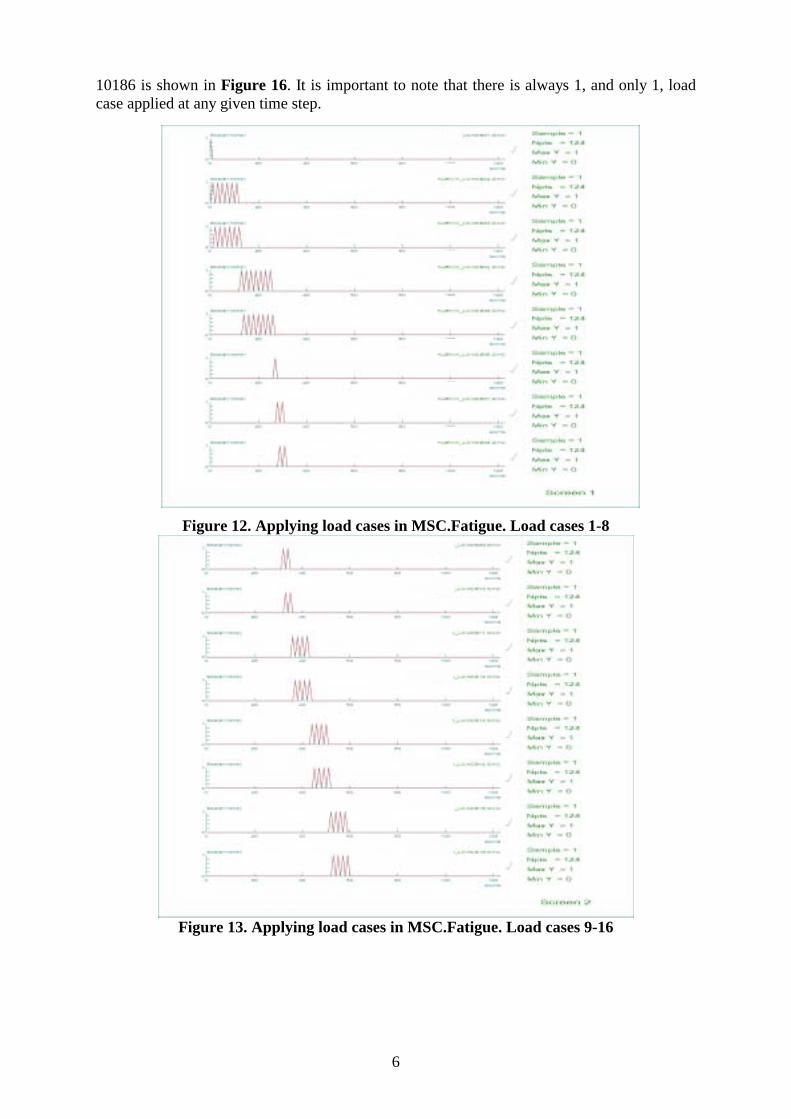
Definition of Mission Profiles in MSC.Fatigue It is not obvious, with MSC.Fatigue, how to set up and apply multiple loadings of the form normally applied to aircraft structures. Table 1 lists the various base load (stress) cases which must be applied. These loadings should be applied sequentially, one at a time. However, MSC.Fatigue expects multiple loadings to be applied simultaneously. The linear superposition of these loadings is then usually achieved with the following equation,
∑
=
k feak
kijkij P
tPt,
,)()(σ
σ
where )(tPk is the force time history, feakP , is the magnitude of the force used to produce the static load case (usually unity) and kij ,σ is the Nastran static stress result at point ij, for load case k. For the purpose of the work reported in this study the mission profile was easily defined by setting up, for each load case, a time series of zeros and ones, with the base load case being applied by specifying 1, and being turned off by specifying 0. These time series
)(1 tP to )(32 tP are shown in the following figures. The resultant stress history at critical node
6
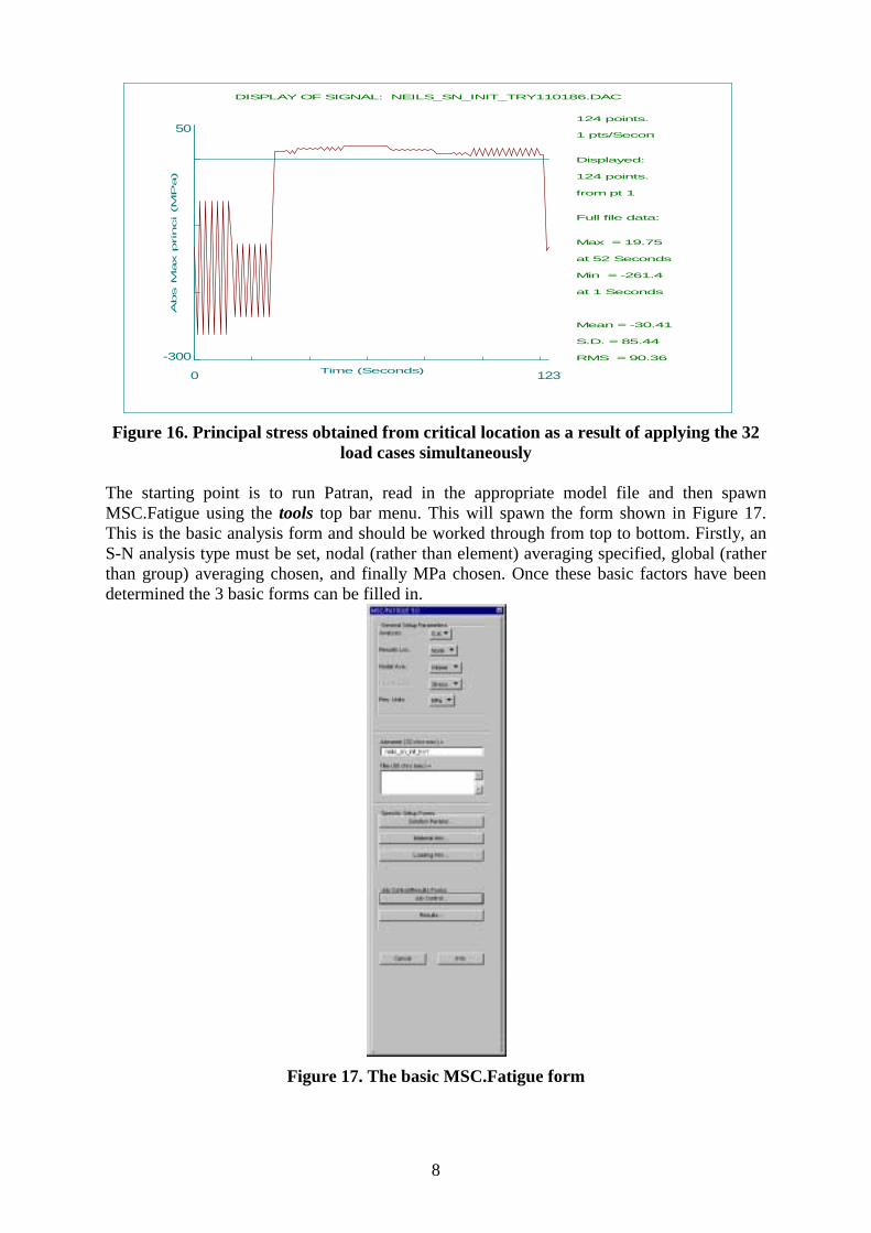
10186 is shown in Figure 16. It is important to note that there is always 1, and only 1, load case applied at any given time step.
Figure 12. Applying load cases in MSC.Fatigue. Load cases 1-8
Figure 13. Applying load cases in MSC.Fatigue. Load cases 9-16
7
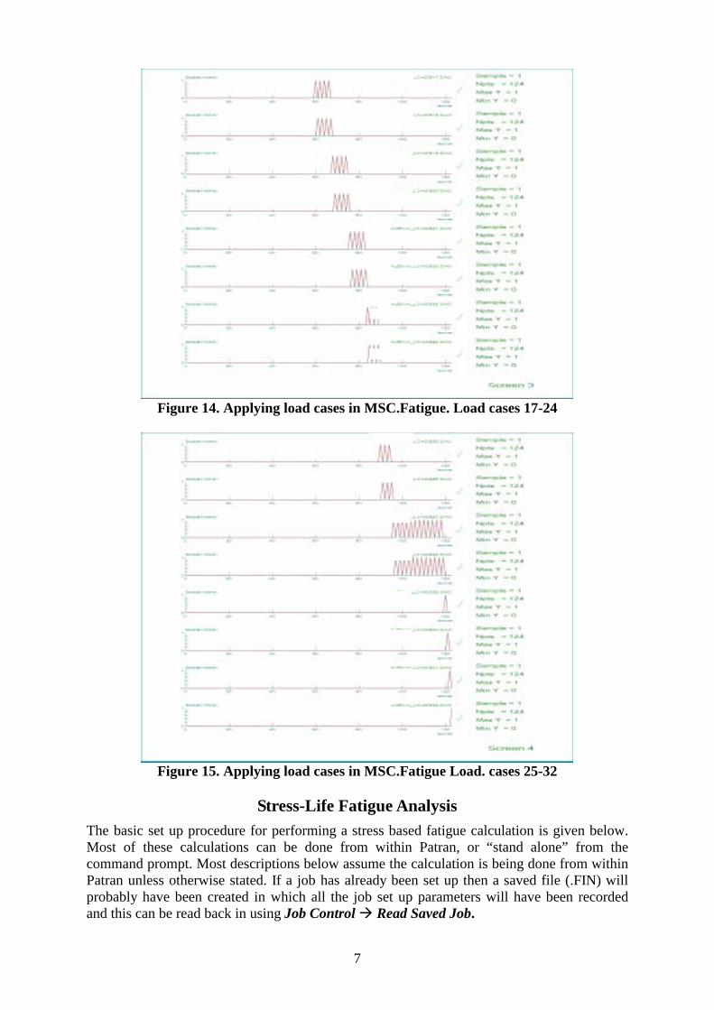
Figure 14. Applying load cases in MSC.Fatigue. Load cases 17-24
Figure 15. Applying load cases in MSC.Fatigue Load. cases 25-32
Stress-Life Fatigue Analysis
The basic set up procedure for performing a stress based fatigue calculation is given below. Most of these calculations can be done from within Patran, or “stand alone” from the command prompt. Most descriptions below assume the calculation is being done from within Patran unless otherwise stated. If a job has already been set up then a saved file (.FIN) will probably have been created in which all the job set up parameters will have been recorded and this can be read back in using Job Control ! Read Saved Job.
8
50
-300
1230
Abs M
ax p
rinci (M
Pa)
Time (Seconds)
DISPLAY OF SIGNAL: NEILS_SN_INIT_TRY110186.DAC
124 points.
1 pts/Secon
Displayed:
124 points.
from pt 1
Full file data:
Max = 19.75
at 52 Seconds
Min = -261.4
at 1 Seconds
Mean = -30.41
S.D. = 85.44
RMS = 90.36
Figure 16. Principal stress obtained from critical location as a result of applying the 32
load cases simultaneously The starting point is to run Patran, read in the appropriate model file and then spawn MSC.Fatigue using the tools top bar menu. This will spawn the form shown in Figure 17. This is the basic analysis form and should be worked through from top to bottom. Firstly, an S-N analysis type must be set, nodal (rather than element) averaging specified, global (rather than group) averaging chosen, and finally MPa chosen. Once these basic factors have been determined the 3 basic forms can be filled in.
Figure 17. The basic MSC.Fatigue form
9
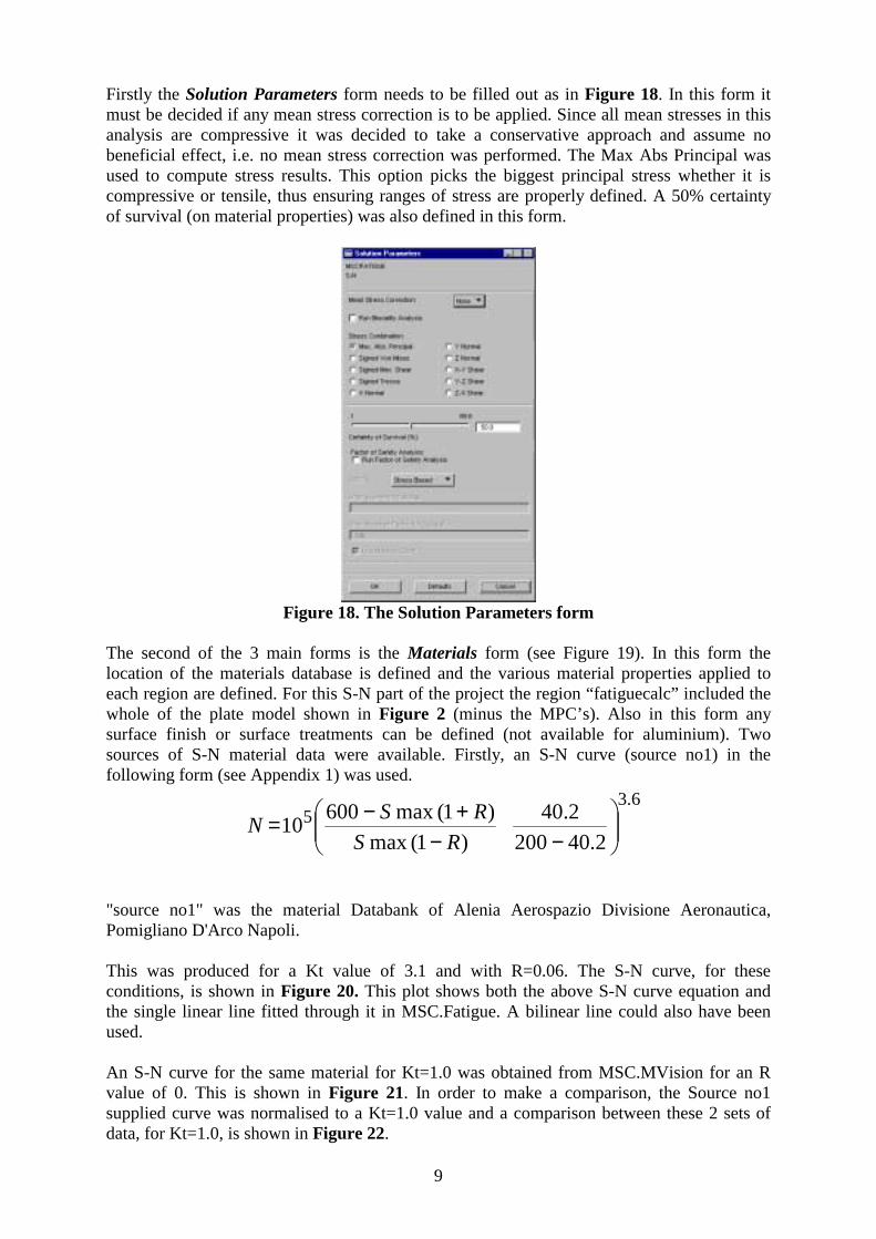
Firstly the Solution Parameters form needs to be filled out as in Figure 18. In this form it must be decided if any mean stress correction is to be applied. Since all mean stresses in this analysis are compressive it was decided to take a conservative approach and assume no beneficial effect, i.e. no mean stress correction was performed. The Max Abs Principal was used to compute stress results. This option picks the biggest principal stress whether it is compressive or tensile, thus ensuring ranges of stress are properly defined. A 50% certainty of survival (on material properties) was also defined in this form.
Figure 18. The Solution Parameters form
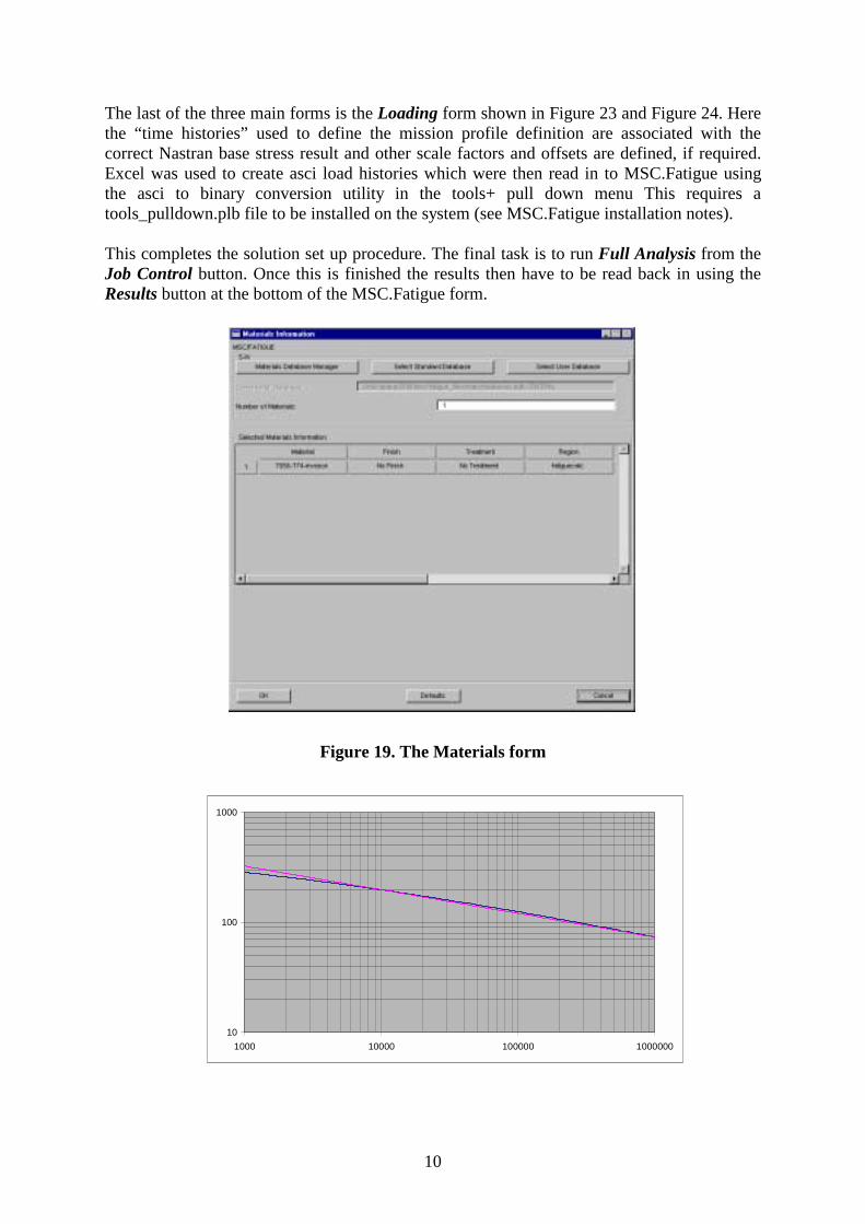
The second of the 3 main forms is the Materials form (see Figure 19). In this form the location of the materials database is defined and the various material properties applied to each region are defined. For this S-N part of the project the region “fatiguecalc” included the whole of the plate model shown in Figure 2 (minus the MPC’s). Also in this form any surface finish or surface treatments can be defined (not available for aluminium). Two sources of S-N material data were available. Firstly, an S-N curve (source no1) in the following form (see Appendix 1) was used.
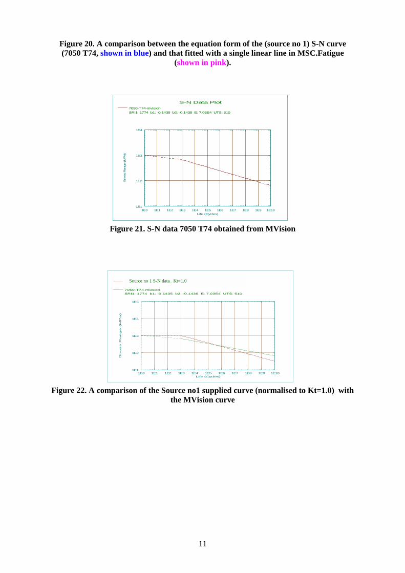
"source no1" was the material Databank of Alenia Aerospazio Divisione Aeronautica, Pomigliano D'Arco Napoli. This was produced for a Kt value of 3.1 and with R=0.06. The S-N curve, for these conditions, is shown in Figure 20. This plot shows both the above S-N curve equation and the single linear line fitted through it in MSC.Fatigue. A bilinear line could also have been used. An S-N curve for the same material for Kt=1.0 was obtained from MSC.MVision for an R value of 0. This is shown in Figure 21. In order to make a comparison, the Source no1 supplied curve was normalised to a Kt=1.0 value and a comparison between these 2 sets of data, for Kt=1.0, is shown in Figure 22.
6.35
2.402002.40
)1(max)1(max60010
−−
+−=RS
RSN
10
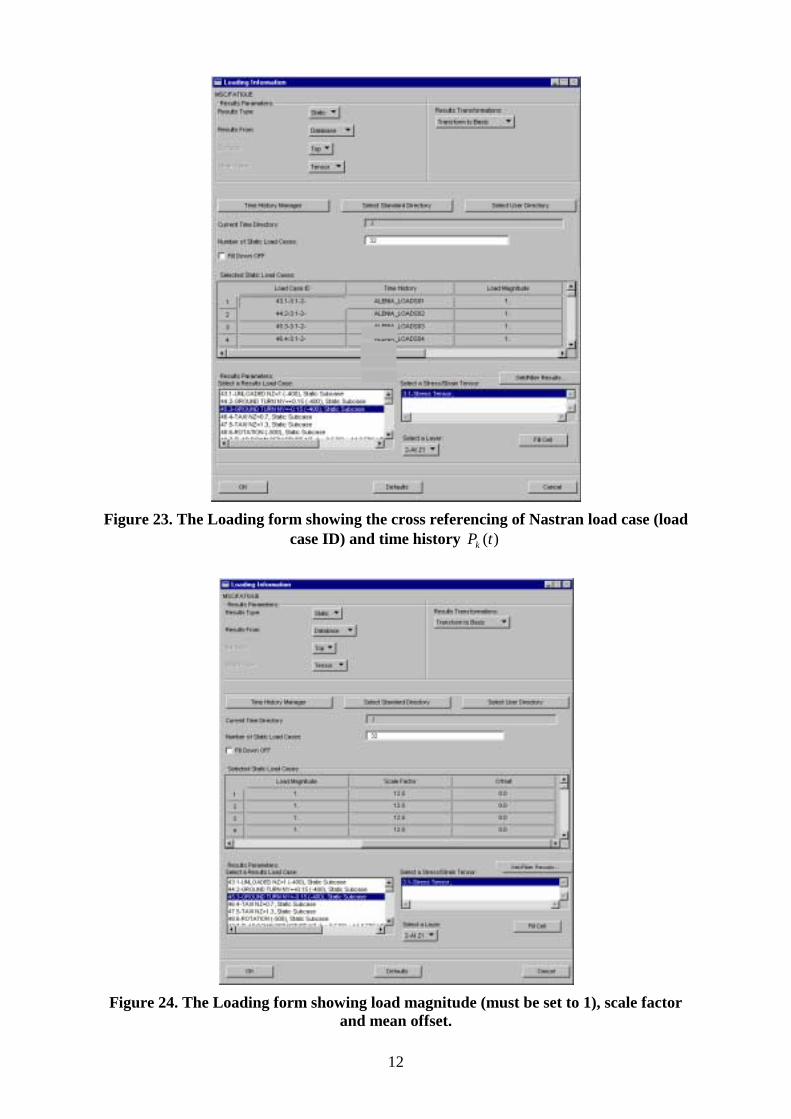
The last of the three main forms is the Loading form shown in Figure 23 and Figure 24. Here the “time histories” used to define the mission profile definition are associated with the correct Nastran base stress result and other scale factors and offsets are defined, if required. Excel was used to create asci load histories which were then read in to MSC.Fatigue using the asci to binary conversion utility in the tools+ pull down menu This requires a tools_pulldown.plb file to be installed on the system (see MSC.Fatigue installation notes). This completes the solution set up procedure. The final task is to run Full Analysis from the Job Control button. Once this is finished the results then have to be read back in using the Results button at the bottom of the MSC.Fatigue form.
Figure 19. The Materials form
10
100
1000
1000 10000 100000 1000000
11
Figure 20. A comparison between the equation form of the (source no 1) S-N curve (7050 T74, shown in blue) and that fitted with a single linear line in MSC.Fatigue
(shown in pink).
S-N Data Plot7050-T74-mvisionSRI1: 1774 b1: -0.1435 b2: -0.1435 E: 7.03E4 UTS: 510
1E1
1E2
1E3
1E4
Stre
ss R
ange
(MPa)
1E0 1E1 1E2 1E3 1E4 1E5 1E6 1E7 1E8 1E9 1E10Life (Cycles)
Figure 21. S-N data 7050 T74 obtained from MVision
S-N Data PlotAlenia_S-N_data_Kt=1.0SRI1: 4449 b1: -0.215 b2: -0.215 E: 7.03E4 UTS: 510 7050-T74-mvisionSRI1: 1774 b1: -0.1435 b2: -0.1435 E: 7.03E4 UTS: 510
1E1
1E2
1E3
1E4
1E5
Str
ess R
an
ge (
MP
a)
1E0 1E1 1E2 1E3 1E4 1E5 1E6 1E7 1E8 1E9 1E10Life (Cycles)
Figure 22. A comparison of the Source no1 supplied curve (normalised to Kt=1.0) with
the MVision curve
Source no 1 S-N data_ Kt=1.0
12
Figure 23. The Loading form showing the cross referencing of Nastran load case (load
case ID) and time history )(tPk
Figure 24. The Loading form showing load magnitude (must be set to 1), scale factor
and mean offset.
13
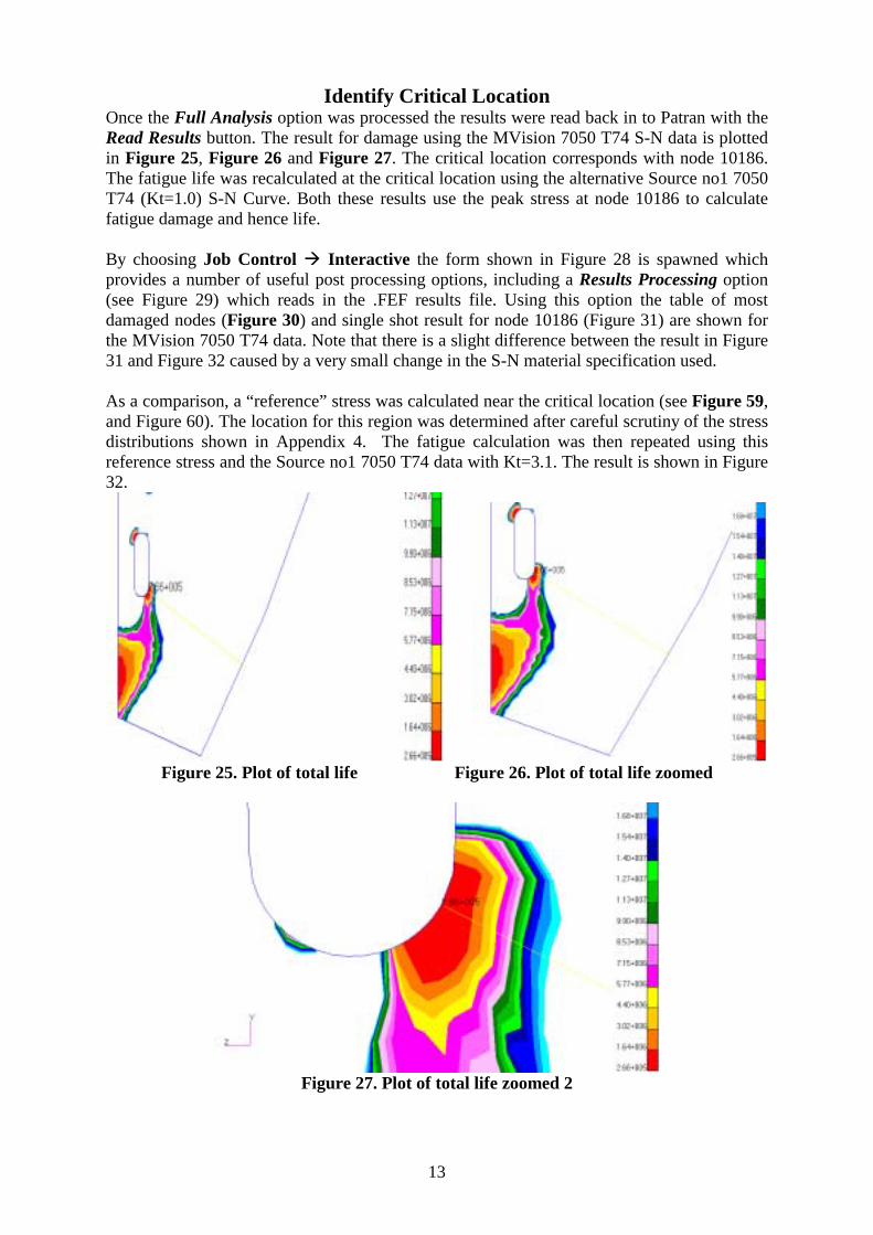
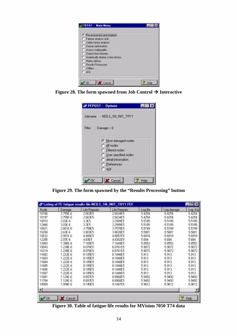
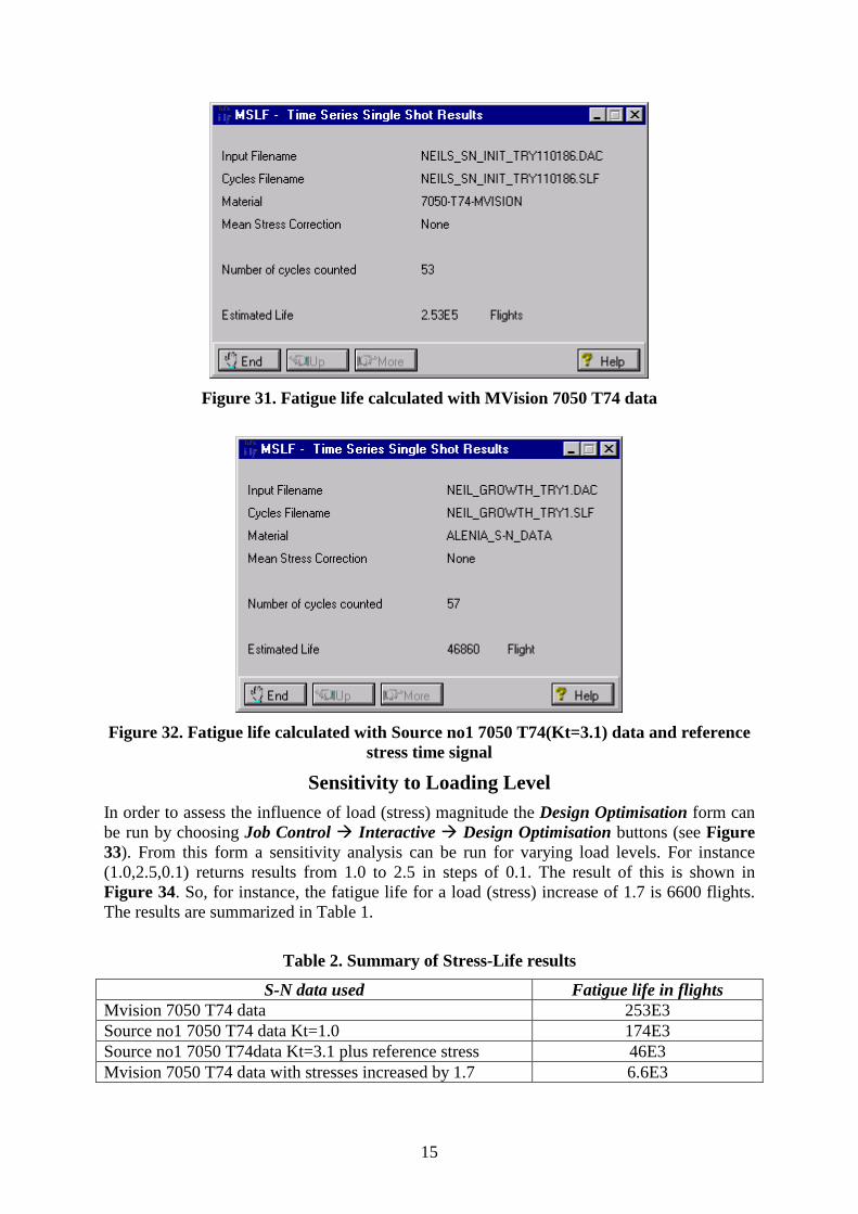
Identify Critical Location Once the Full Analysis option was processed the results were read back in to Patran with the Read Results button. The result for damage using the MVision 7050 T74 S-N data is plotted in Figure 25, Figure 26 and Figure 27. The critical location corresponds with node 10186. The fatigue life was recalculated at the critical location using the alternative Source no1 7050 T74 (Kt=1.0) S-N Curve. Both these results use the peak stress at node 10186 to calculate fatigue damage and hence life. By choosing Job Control ! Interactive the form shown in Figure 28 is spawned which provides a number of useful post processing options, including a Results Processing option (see Figure 29) which reads in the .FEF results file. Using this option the table of most damaged nodes (Figure 30) and single shot result for node 10186 (Figure 31) are shown for the MVision 7050 T74 data. Note that there is a slight difference between the result in Figure 31 and Figure 32 caused by a very small change in the S-N material specification used. As a comparison, a “reference” stress was calculated near the critical location (see Figure 59, and Figure 60). The location for this region was determined after careful scrutiny of the stress distributions shown in Appendix 4. The fatigue calculation was then repeated using this reference stress and the Source no1 7050 T74 data with Kt=3.1. The result is shown in Figure 32.
Figure 25. Plot of total life Figure 26. Plot of total life zoomed
Figure 27. Plot of total life zoomed 2
14
Figure 28. The form spawned from Job Control !!!! Interactive
Figure 29. The form spawned by the “Results Processing” button
Figure 30. Table of fatigue life results for MVision 7050 T74 data
15
Figure 31. Fatigue life calculated with MVision 7050 T74 data
Figure 32. Fatigue life calculated with Source no1 7050 T74(Kt=3.1) data and reference
stress time signal
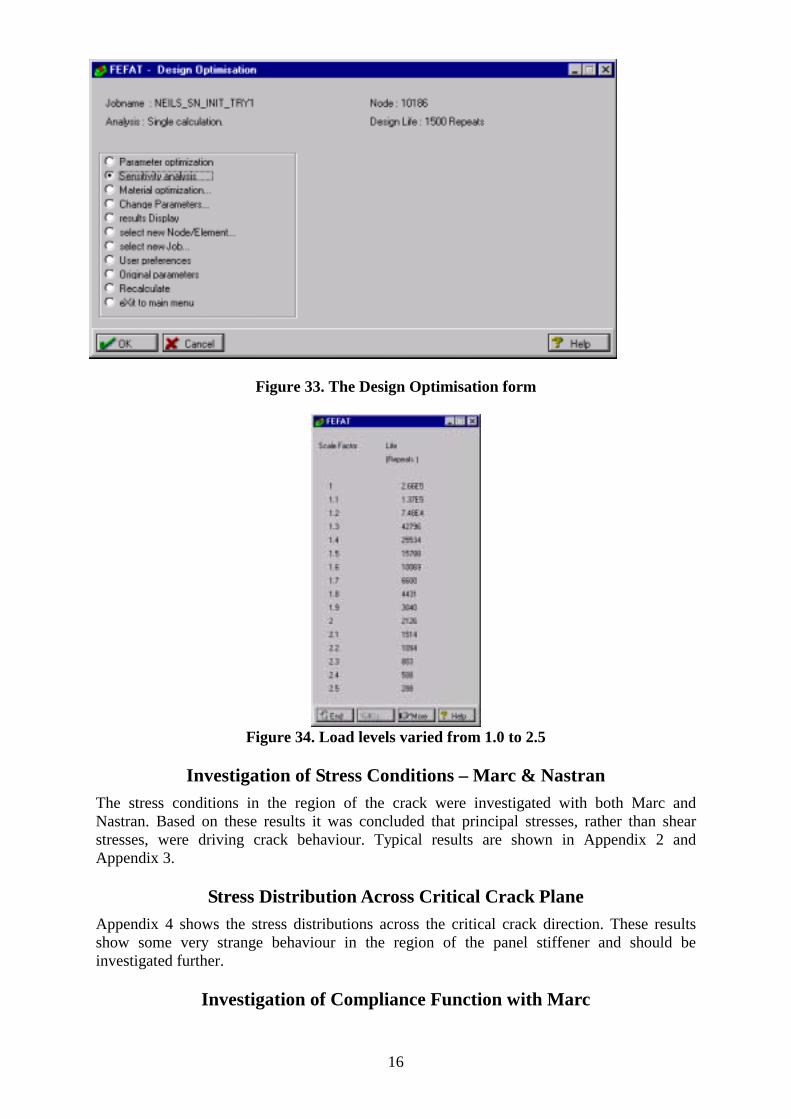
Sensitivity to Loading Level In order to assess the influence of load (stress) magnitude the Design Optimisation form can be run by choosing Job Control ! Interactive ! Design Optimisation buttons (see Figure 33). From this form a sensitivity analysis can be run for varying load levels. For instance (1.0,2.5,0.1) returns results from 1.0 to 2.5 in steps of 0.1. The result of this is shown in Figure 34. So, for instance, the fatigue life for a load (stress) increase of 1.7 is 6600 flights. The results are summarized in Table 1.
Table 2. Summary of Stress-Life results
S-N data used Fatigue life in flights Mvision 7050 T74 data 253E3 Source no1 7050 T74 data Kt=1.0 174E3 Source no1 7050 T74data Kt=3.1 plus reference stress 46E3 Mvision 7050 T74 data with stresses increased by 1.7 6.6E3
16
Figure 33. The Design Optimisation form
Figure 34. Load levels varied from 1.0 to 2.5
Investigation of Stress Conditions – Marc & Nastran
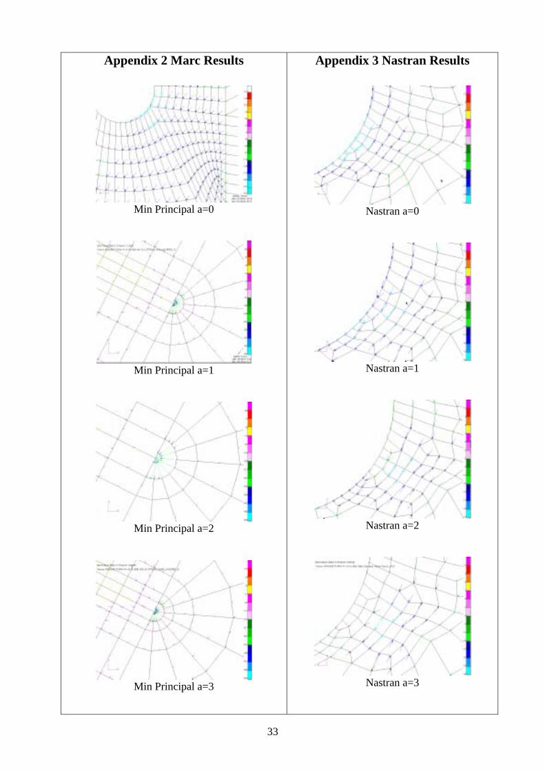
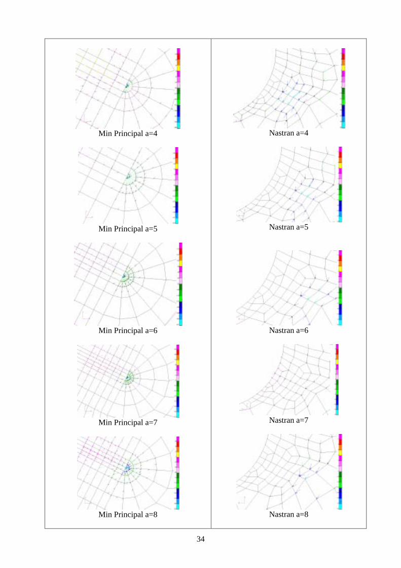
The stress conditions in the region of the crack were investigated with both Marc and Nastran. Based on these results it was concluded that principal stresses, rather than shear stresses, were driving crack behaviour. Typical results are shown in Appendix 2 and Appendix 3.
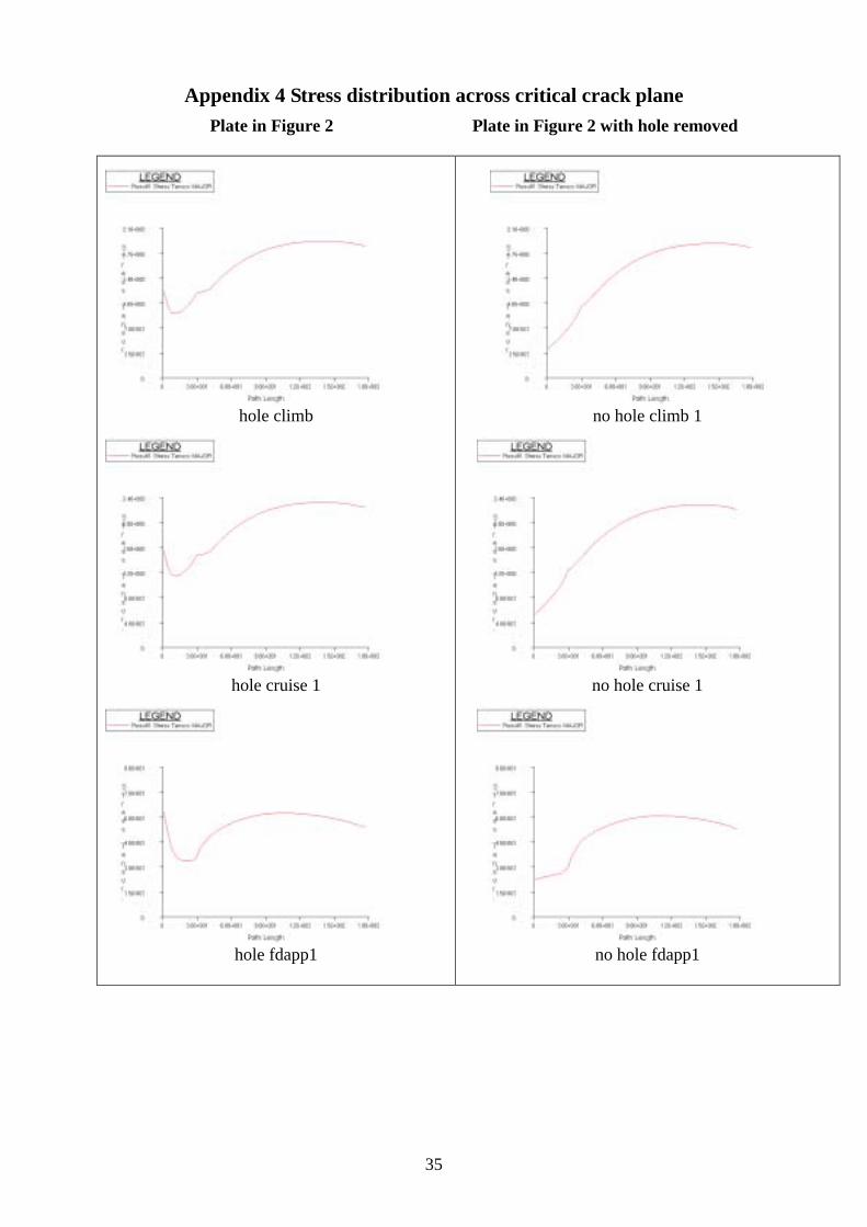
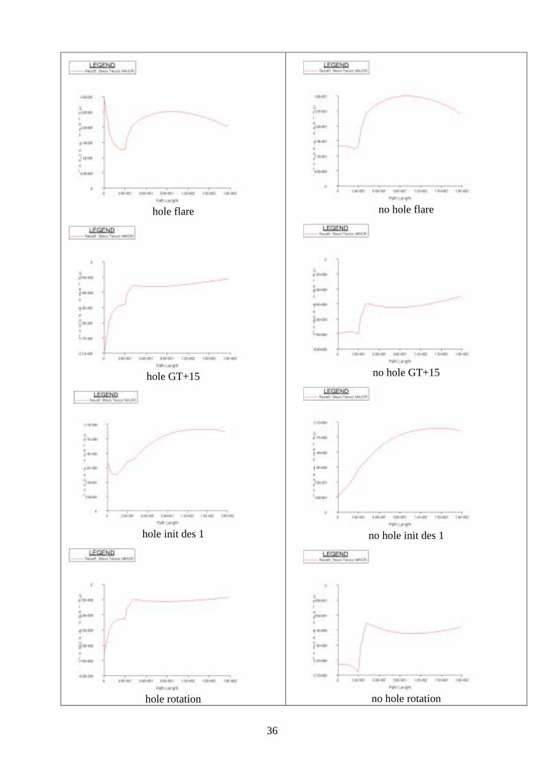
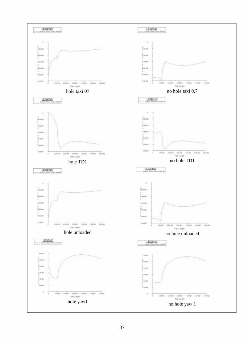
Stress Distribution Across Critical Crack Plane Appendix 4 shows the stress distributions across the critical crack direction. These results show some very strange behaviour in the region of the panel stiffener and should be investigated further.
Investigation of Compliance Function with Marc
17
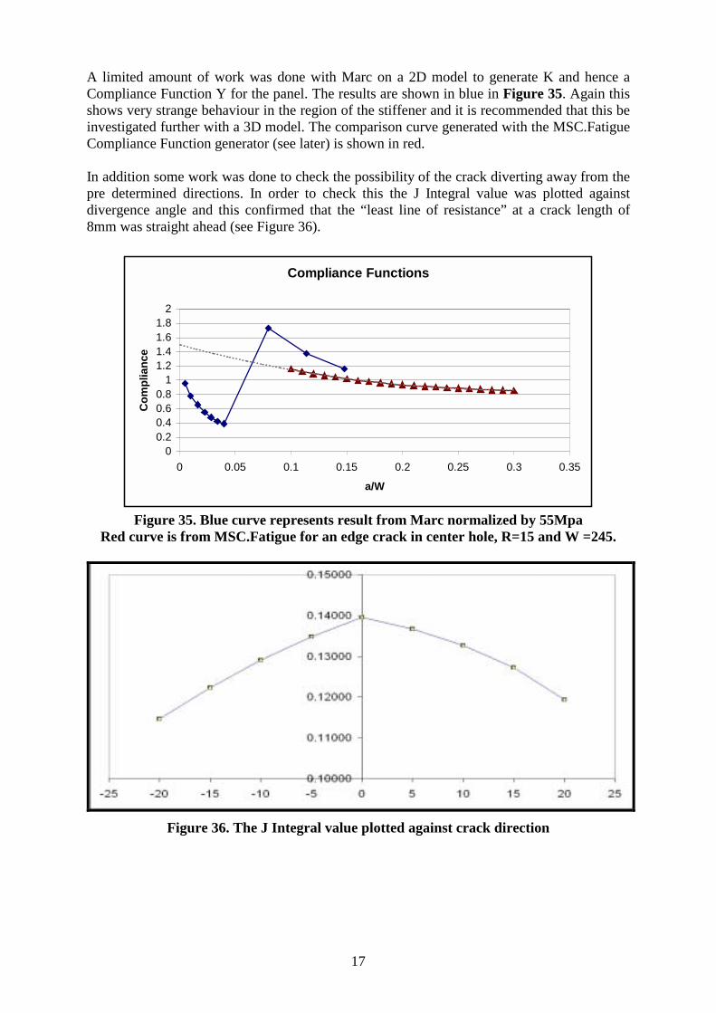
A limited amount of work was done with Marc on a 2D model to generate K and hence a Compliance Function Y for the panel. The results are shown in blue in Figure 35. Again this shows very strange behaviour in the region of the stiffener and it is recommended that this be investigated further with a 3D model. The comparison curve generated with the MSC.Fatigue Compliance Function generator (see later) is shown in red. In addition some work was done to check the possibility of the crack diverting away from the pre determined directions. In order to check this the J Integral value was plotted against divergence angle and this confirmed that the “least line of resistance” at a crack length of 8mm was straight ahead (see Figure 36).
Compliance Functions
00.20.40.60.8
11.21.41.61.8
2
0 0.05 0.1 0.15 0.2 0.25 0.3 0.35
a/W
Com
plia
nce
Figure 35. Blue curve represents result from Marc normalized by 55Mpa
Red curve is from MSC.Fatigue for an edge crack in center hole, R=15 and W =245.
Figure 36. The J Integral value plotted against crack direction
18
Crack Growth Calculation With MSC.Fatigue
The Concept of Stress Intensity
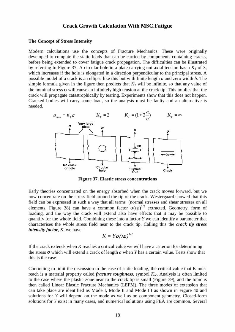
Modern calculations use the concepts of Fracture Mechanics. These were originally developed to compute the static loads that can be carried by components containing cracks, before being extended to cover fatigue crack propagation. The difficulties can be illustrated by referring to Figure 37. A circular hole in a plate carrying uni-axial tension has a KT of 3, which increases if the hole is elongated in a direction perpendicular to the principal stress. A possible model of a crack is an ellipse like this but with finite length a and zero width b. The simple formula given in the figure then predicts that KT will be infinite, so that any value of the nominal stress σ will cause an infinitely high tension at the crack tip. This implies that the crack will propagate catastrophically by tearing. Experiments show that this does not happen. Cracked bodies will carry some load, so the analysis must be faulty and an alternative is needed.
σσ TK=max 3=TK )21(baKT += ∞=TK
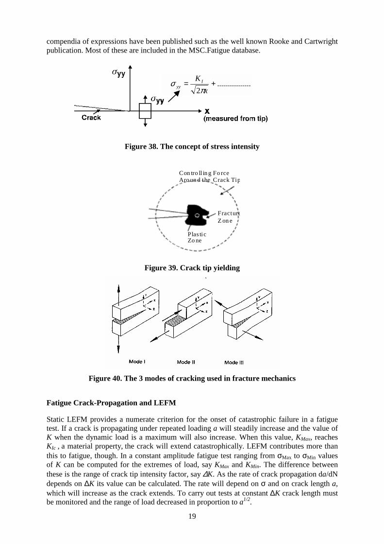
Figure 37. Elastic stress concentrations Early theories concentrated on the energy absorbed when the crack moves forward, but we now concentrate on the stress field around the tip of the crack. Westergaard showed that this field can be expressed in such a way that all terms (normal stresses and shear stresses on all elements, Figure 38) can have a common factor σ(πa)1/2 extracted. Geometry, form of loading, and the way the crack will extend also have effects that it may be possible to quantify for the whole field. Combining these into a factor Y we can identify a parameter that characterises the whole stress field near to the crack tip. Calling this the crack tip stress intensity factor, K, we have:-
K = Yσ(πa)1/2 If the crack extends when K reaches a critical value we will have a criterion for determining the stress σ which will extend a crack of length a when Y has a certain value. Tests show that this is the case. Continuing to limit the discussion to the case of static loading, the critical value that K must reach is a material property called fracture toughness, symbol KIc. Analysis is often limited to the case where the plastic zone near to the crack tip is small (Figure 39), and the topic is then called Linear Elastic Fracture Mechanics (LEFM). The three modes of extension that can take place are identified as Mode I, Mode II and Mode III as shown in Figure 40 and solutions for Y will depend on the mode as well as on component geometry. Closed-form solutions for Y exist in many cases, and numerical solutions using FEA are common. Several
19
compendia of expressions have been published such as the well known Rooke and Cartwright publication. Most of these are included in the MSC.Fatigue database.
Figure 38. The concept of stress intensity
FractureZ on e
Plas ti cZo ne
Con tro ll in g Fo rceAro un d the Crack Tip
Figure 39. Crack tip yielding
Figure 40. The 3 modes of cracking used in fracture mechanics
Fatigue Crack-Propagation and LEFM
Static LEFM provides a numerate criterion for the onset of catastrophic failure in a fatigue test. If a crack is propagating under repeated loading a will steadily increase and the value of K when the dynamic load is a maximum will also increase. When this value, KMax, reaches KIc , a material property, the crack will extend catastrophically. LEFM contributes more than this to fatigue, though. In a constant amplitude fatigue test ranging from σMax to σMin values of K can be computed for the extremes of load, say KMax and KMin. The difference between these is the range of crack tip intensity factor, say ∆K. As the rate of crack propagation da/dN depends on ∆K its value can be calculated. The rate will depend on σ and on crack length a, which will increase as the crack extends. To carry out tests at constant ∆K crack length must be monitored and the range of load decreased in proportion to a1/2.
.................2
+=x
K Iyy π
σ
20
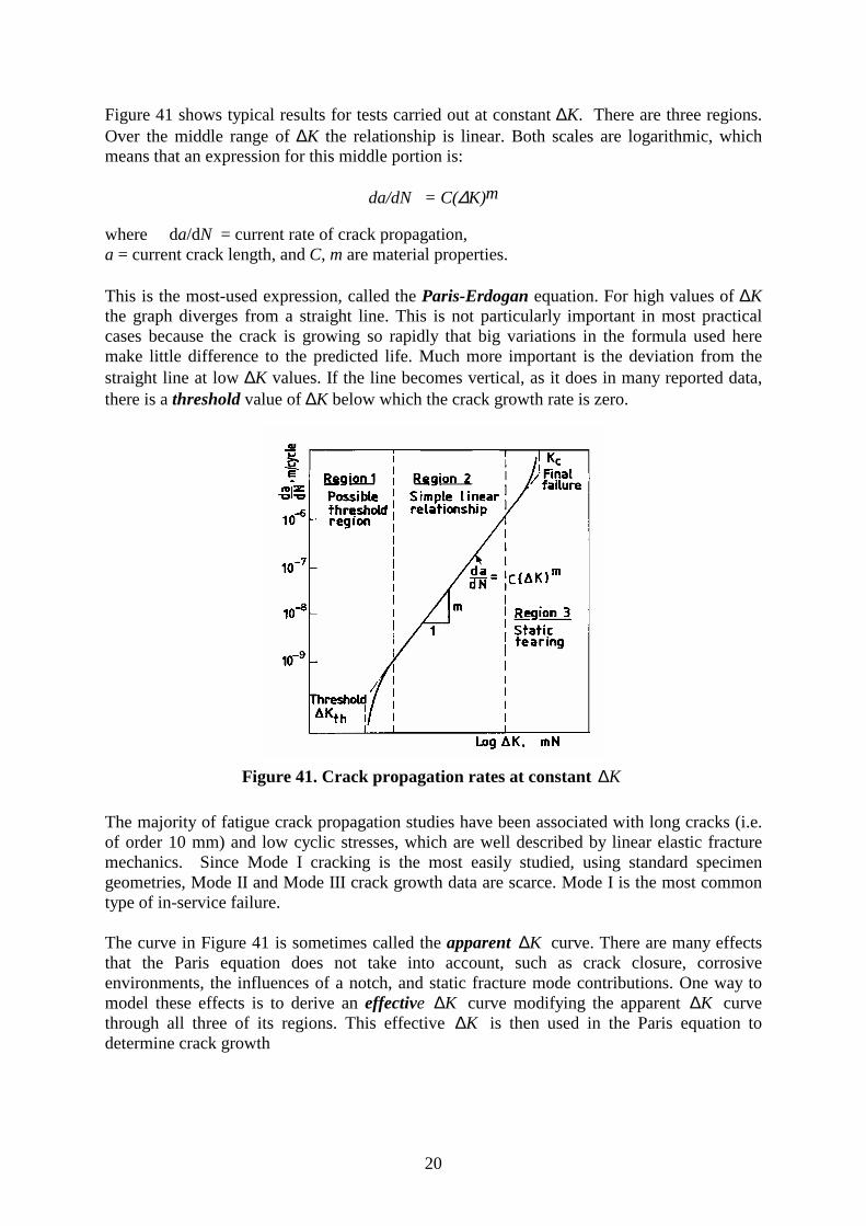
Figure 41 shows typical results for tests carried out at constant ∆K. There are three regions. Over the middle range of ∆K the relationship is linear. Both scales are logarithmic, which means that an expression for this middle portion is:
da/dN = C(∆K)m where da/dN = current rate of crack propagation, a = current crack length, and C, m are material properties. This is the most-used expression, called the Paris-Erdogan equation. For high values of ∆K the graph diverges from a straight line. This is not particularly important in most practical cases because the crack is growing so rapidly that big variations in the formula used here make little difference to the predicted life. Much more important is the deviation from the straight line at low ∆K values. If the line becomes vertical, as it does in many reported data, there is a threshold value of ∆K below which the crack growth rate is zero.
Figure 41. Crack propagation rates at constant K∆ The majority of fatigue crack propagation studies have been associated with long cracks (i.e. of order 10 mm) and low cyclic stresses, which are well described by linear elastic fracture mechanics. Since Mode I cracking is the most easily studied, using standard specimen geometries, Mode II and Mode III crack growth data are scarce. Mode I is the most common type of in-service failure. The curve in Figure 41 is sometimes called the apparent K∆ curve. There are many effects that the Paris equation does not take into account, such as crack closure, corrosive environments, the influences of a notch, and static fracture mode contributions. One way to model these effects is to derive an effective K∆ curve modifying the apparent K∆ curve through all three of its regions. This effective K∆ is then used in the Paris equation to determine crack growth
21
Stresss Intensity Factor K Versus Compliance-Function Y
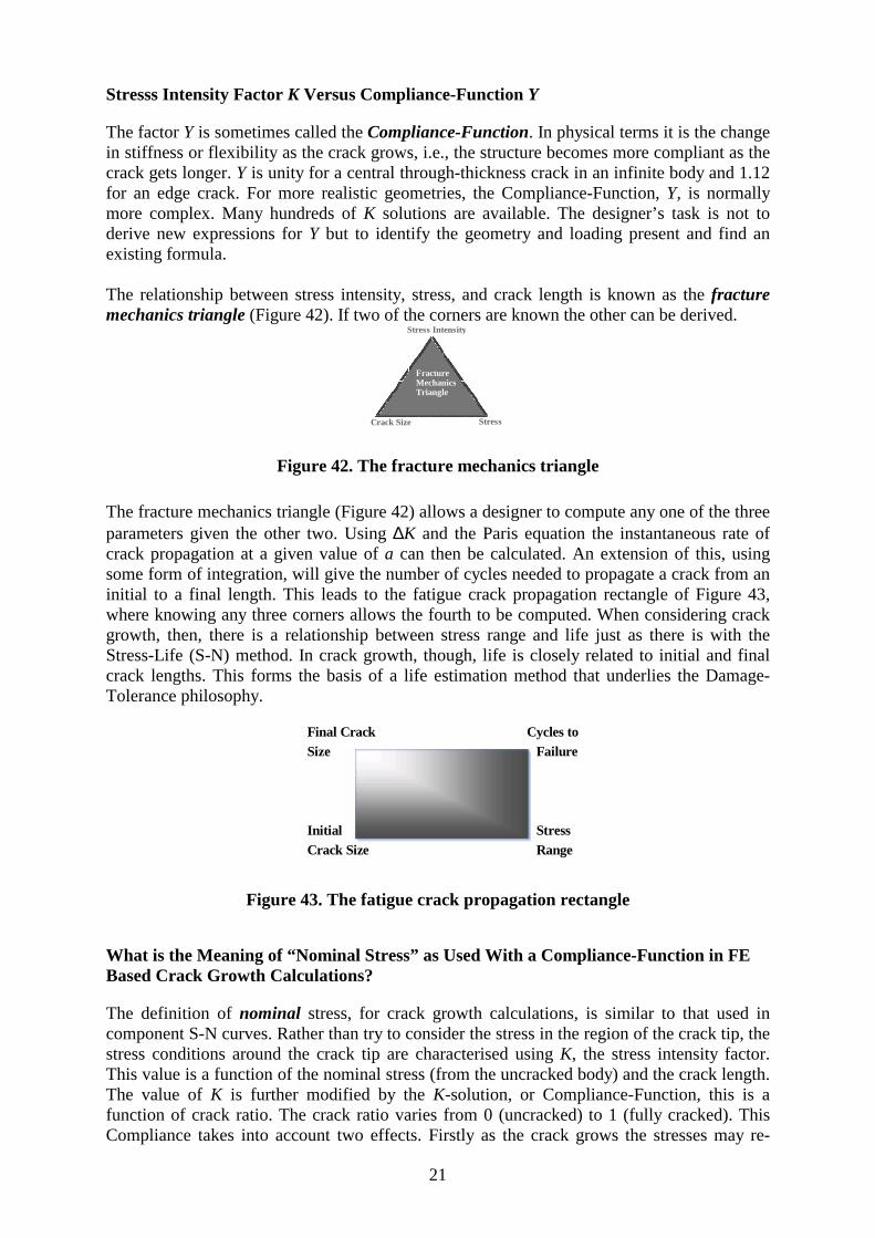
The factor Y is sometimes called the Compliance-Function. In physical terms it is the change in stiffness or flexibility as the crack grows, i.e., the structure becomes more compliant as the crack gets longer. Y is unity for a central through-thickness crack in an infinite body and 1.12 for an edge crack. For more realistic geometries, the Compliance-Function, Y, is normally more complex. Many hundreds of K solutions are available. The designer’s task is not to derive new expressions for Y but to identify the geometry and loading present and find an existing formula. The relationship between stress intensity, stress, and crack length is known as the fracture mechanics triangle (Figure 42). If two of the corners are known the other can be derived.
Stress Intensity
StressCrack Size
Fracture MechanicsTriangle
Figure 42. The fracture mechanics triangle The fracture mechanics triangle (Figure 42) allows a designer to compute any one of the three parameters given the other two. Using ∆K and the Paris equation the instantaneous rate of crack propagation at a given value of a can then be calculated. An extension of this, using some form of integration, will give the number of cycles needed to propagate a crack from an initial to a final length. This leads to the fatigue crack propagation rectangle of Figure 43, where knowing any three corners allows the fourth to be computed. When considering crack growth, then, there is a relationship between stress range and life just as there is with the Stress-Life (S-N) method. In crack growth, though, life is closely related to initial and final crack lengths. This forms the basis of a life estimation method that underlies the Damage-Tolerance philosophy.
Final CrackSize
InitialCrack Size
Cycles toFailure
StressRange
Figure 43. The fatigue crack propagation rectangle
What is the Meaning of “Nominal Stress” as Used With a Compliance-Function in FE Based Crack Growth Calculations?
The definition of nominal stress, for crack growth calculations, is similar to that used in component S-N curves. Rather than try to consider the stress in the region of the crack tip, the stress conditions around the crack tip are characterised using K, the stress intensity factor. This value is a function of the nominal stress (from the uncracked body) and the crack length. The value of K is further modified by the K-solution, or Compliance-Function, this is a function of crack ratio. The crack ratio varies from 0 (uncracked) to 1 (fully cracked). This Compliance takes into account two effects. Firstly as the crack grows the stresses may re-

22
distribute and secondly the crack may be growing into higher or lower-stressed areas. So it is very important to use the correct “nominal” stress.
Using Fracture Mechanics in Damage-Tolerant Design.
In one version of Damage-Tolerant design the initial crack length ai is determined by the longest crack likely to be missed at inspection, and the final crack length af is the one which would cause catastrophic failure. If the applied fatigue loading is constant-amplitude, the steps in the calculation are: (i) Estimate the size of crack likely to be present in the component when it is first put into service, ai. (ii) From a measured value of KIc, estimate the maximum crack length, af, which the component will tolerate when the applied stress reaches maximum tension. An expression for the crack-tip stress intensity factor will be needed. (iii) Using the same expression for crack-tip stress intensity factor, calculate ∆K. (iv) Substitute ∆K into the Paris equation to obtain a crack propagation rate. This will put da/dN in terms of crack length a. (v) Integrate this equation between a = ai and a = af to give the number of cycles needed to grow a crack from ai to af. This is the predicted life of the component. A classical integration is adequate if the Compliance Function is constant. Other Compliance Functions will require a numerical integration, as will any non-constant amplitude signal.
Implementation in MSC.Fatigue
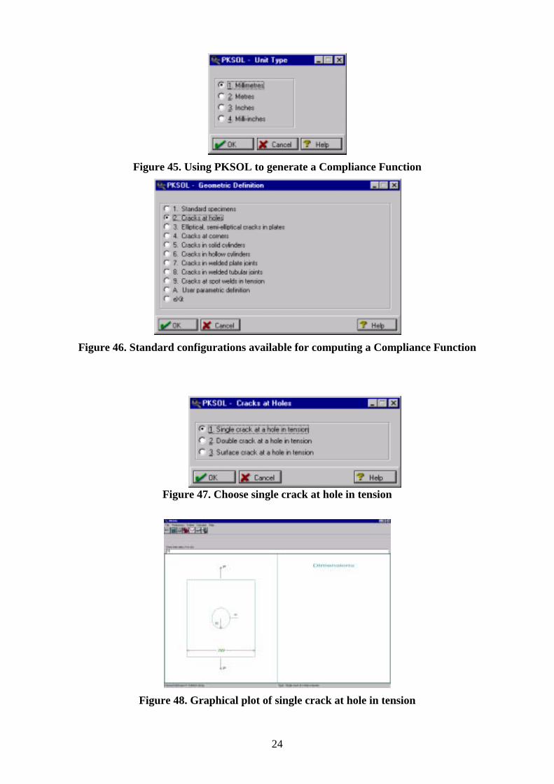
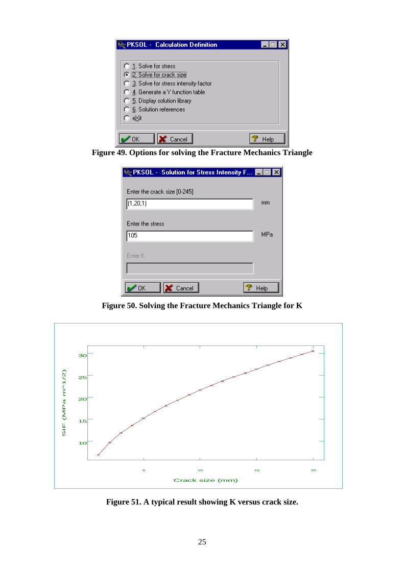
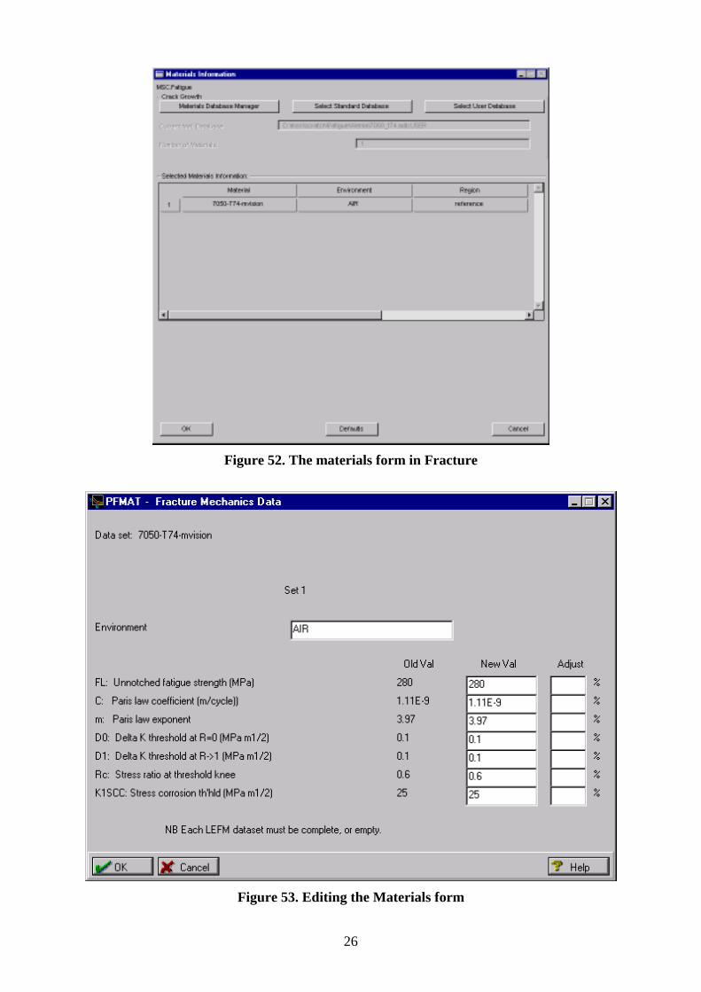
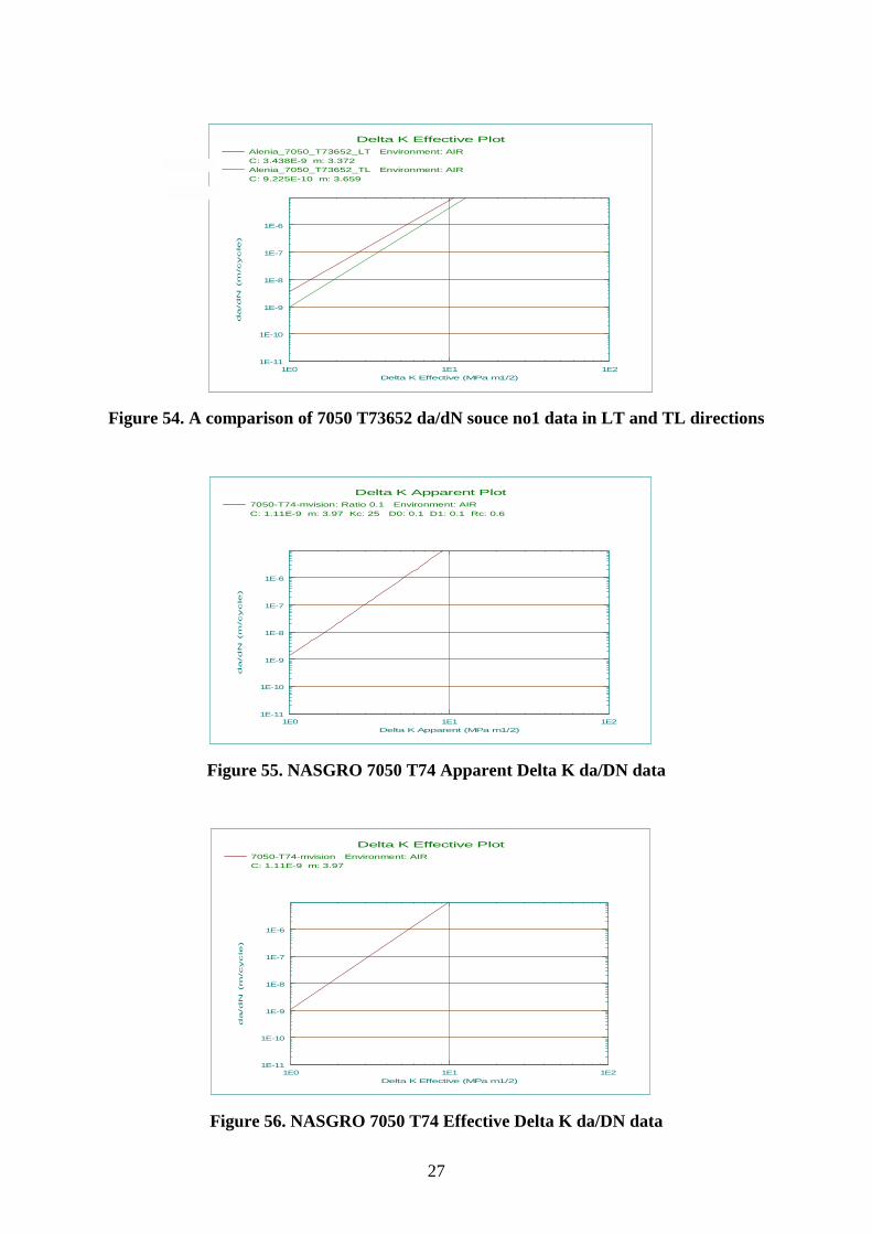
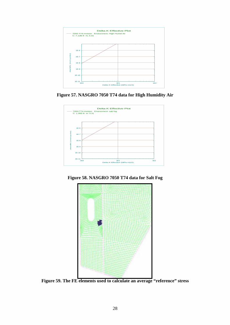
Again the starting point for an MSC.Fatigue analysis is the MSC.Fatigue form spawned from the tools top bar menu as shown in Figure 44. Now, because Crack Growth has been chosen there is a new button Compliance Function at the top of the form. This allows PKSOL to be accessed which is a useful tool for generating Compliance Functions from a standard library, for entering externally defined CF’s, and also for solving the Fracture Mechanics Triangle to obtain, for instance, K from crack length and stress level. Examples of this are shown in Figure 45 to Figure 51. Once a Compliance Function is available the rest of the MSC.Fatigue forms can be generated in a very similar way to the S-N approach. Figure 52 shows the Materials form. In this form the appropriate da/dN curve is specified. da/dN data is somewhat more complicated than S-N data, allowing a number of modifications to be made to deal with, for instance, history effects, crack closure, etc. These were all turned off in the analysis so that a standard Paris type crack growth calculation was performed. In order to ensure that all these effects are turned off the values for D0 and D1 in the form (see Figure 53) have to be set to very low values, say 0.1 (the reader is referred to the MSC.Fatigue User Manual for more details). The one major difference in the Material form is that the region defined here is the region from which the reference stress is to be calculated. Figure 54 to Figure 58 show the various da/dN curves used. In order to perform a crack growth calculation an appropriate reference stress has to be calculated form the model. This should be representative of the “nominal” stress in the model
23
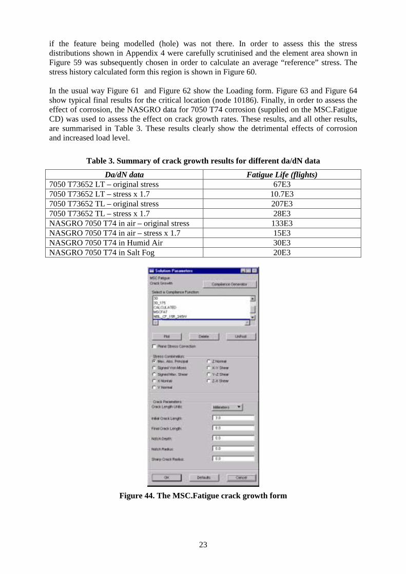
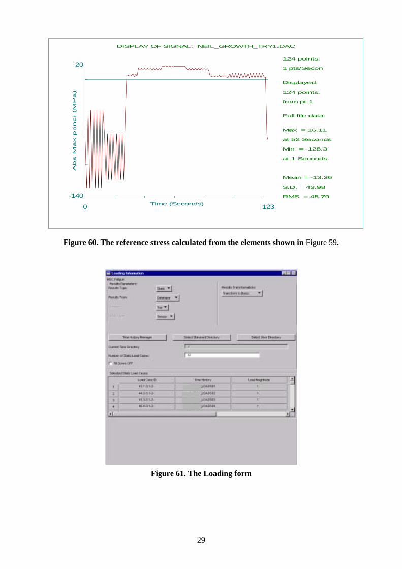
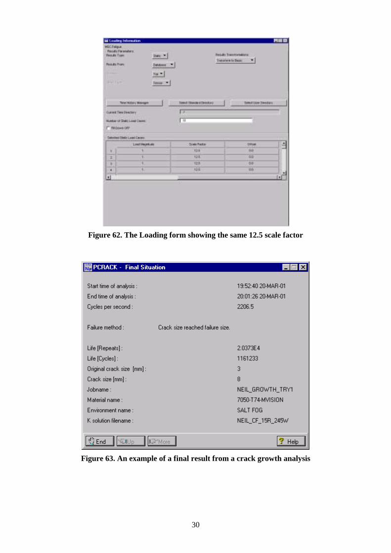
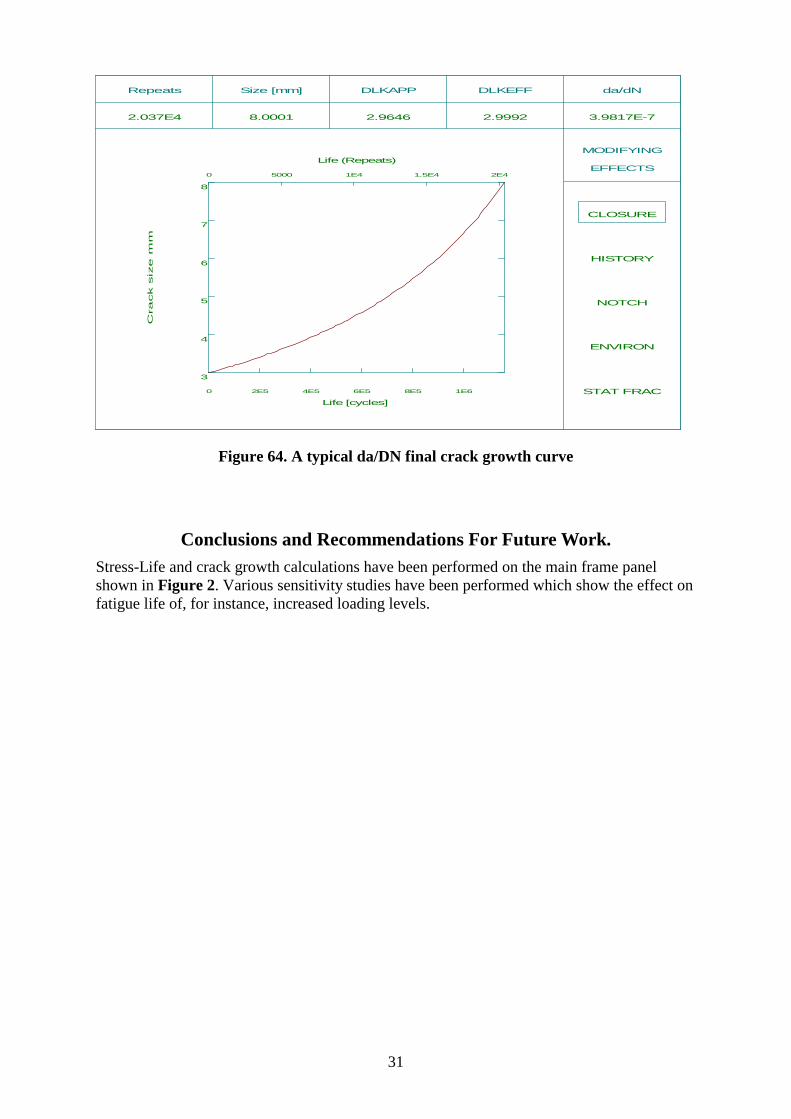
if the feature being modelled (hole) was not there. In order to assess this the stress distributions shown in Appendix 4 were carefully scrutinised and the element area shown in Figure 59 was subsequently chosen in order to calculate an average “reference” stress. The stress history calculated form this region is shown in Figure 60. In the usual way Figure 61 and Figure 62 show the Loading form. Figure 63 and Figure 64 show typical final results for the critical location (node 10186). Finally, in order to assess the effect of corrosion, the NASGRO data for 7050 T74 corrosion (supplied on the MSC.Fatigue CD) was used to assess the effect on crack growth rates. These results, and all other results, are summarised in Table 3. These results clearly show the detrimental effects of corrosion and increased load level.
Table 3. Summary of crack growth results for different da/dN data
Da/dN data Fatigue Life (flights) 7050 T73652 LT – original stress 67E3 7050 T73652 LT – stress x 1.7 10.7E3 7050 T73652 TL – original stress 207E3 7050 T73652 TL – stress x 1.7 28E3 NASGRO 7050 T74 in air – original stress 133E3 NASGRO 7050 T74 in air – stress x 1.7 15E3 NASGRO 7050 T74 in Humid Air 30E3 NASGRO 7050 T74 in Salt Fog 20E3
Figure 44. The MSC.Fatigue crack growth form
24
Figure 45. Using PKSOL to generate a Compliance Function
Figure 46. Standard configurations available for computing a Compliance Function
Figure 47. Choose single crack at hole in tension
Figure 48. Graphical plot of single crack at hole in tension
25
Figure 49. Options for solving the Fracture Mechanics Triangle
Figure 50. Solving the Fracture Mechanics Triangle for K
5 10 15 20
10
15
20
25
30
SIF
(M
Pa
m^1
/2)
Crack size (mm)
Figure 51. A typical result showing K versus crack size.
26
Figure 52. The materials form in Fracture
Figure 53. Editing the Materials form
27
Delta K Effective PlotAlenia_7050_T73652_LT Environment: AIRC: 3.438E-9 m: 3.372 Alenia_7050_T73652_TL Environment: AIRC: 9.225E-10 m: 3.659
1E-11
1E-10
1E-9
1E-8
1E-7
1E-6
da/d
N (
m/c
ycle
)
1E0 1E1 1E2Delta K Effective (MPa m1/2)
Figure 54. A comparison of 7050 T73652 da/dN souce no1 data in LT and TL directions
Delta K Apparent Plot7050-T74-mvision: Ratio 0.1 Environment: AIRC: 1.11E-9 m: 3.97 Kc: 25 D0: 0.1 D1: 0.1 Rc: 0.6
1E-11
1E-10
1E-9
1E-8
1E-7
1E-6
da/d
N (
m/c
ycle
)
1E0 1E1 1E2Delta K Apparent (MPa m1/2)
Figure 55. NASGRO 7050 T74 Apparent Delta K da/DN data
Delta K Effective Plot7050-T74-mvision Environment: AIRC: 1.11E-9 m: 3.97
1E-11
1E-10
1E-9
1E-8
1E-7
1E-6
da/d
N (
m/c
ycle
)
1E0 1E1 1E2Delta K Effective (MPa m1/2)
Figure 56. NASGRO 7050 T74 Effective Delta K da/DN data
28
Delta K Effective Plot
7050-T74-mvision Environment: High Humid AirC: 7.12E-9 m: 3.31
1E-11
1E-10
1E-9
1E-8
1E-7
1E-6
da/d
N (
m/c
ycle
)
1E0 1E1 1E2Delta K Effective (MPa m1/2)
Figure 57. NASGRO 7050 T74 data for High Humidity Air
Delta K Effective Plot
7050-T74-mvision Environment: salt fogC: 1.05E-8 m: 3.31
1E-11
1E-10
1E-9
1E-8
1E-7
1E-6
da
/dN
(m
/cycle
)
1E0 1E1 1E2Delta K Effective (MPa m1/2)
Figure 58. NASGRO 7050 T74 data for Salt Fog
Figure 59. The FE elements used to calculate an average “reference” stress
29
20
-140
1230
Abs M
ax p
rinci (M
Pa)
Time (Seconds)
DISPLAY OF SIGNAL: NEIL_GROWTH_TRY1.DAC
124 points.
1 pts/Secon
Displayed:
124 points.
from pt 1
Full file data:
Max = 16.11
at 52 Seconds
Min = -128.3
at 1 Seconds
Mean = -13.36
S.D. = 43.98
RMS = 45.79
Figure 60. The reference stress calculated from the elements shown in Figure 59.
Figure 61. The Loading form
30
Figure 62. The Loading form showing the same 12.5 scale factor
Figure 63. An example of a final result from a crack growth analysis
31
Repeats Size [mm] DLKAPP DLKEFF da/dN
MODIFYING
EFFECTS
0 2E5 4E5 6E5 8E5 1E6
3
4
5
6
7
8
Cra
ck s
ize
mm
Life [cycles]
Life (Repeats)
0 5000 1E4 1.5E4 2E4
2.037E4 8.0001 2.9646 2.9992 3.9817E-7
CLOSURE
HISTORY
NOTCH
ENVIRON
STAT FRAC
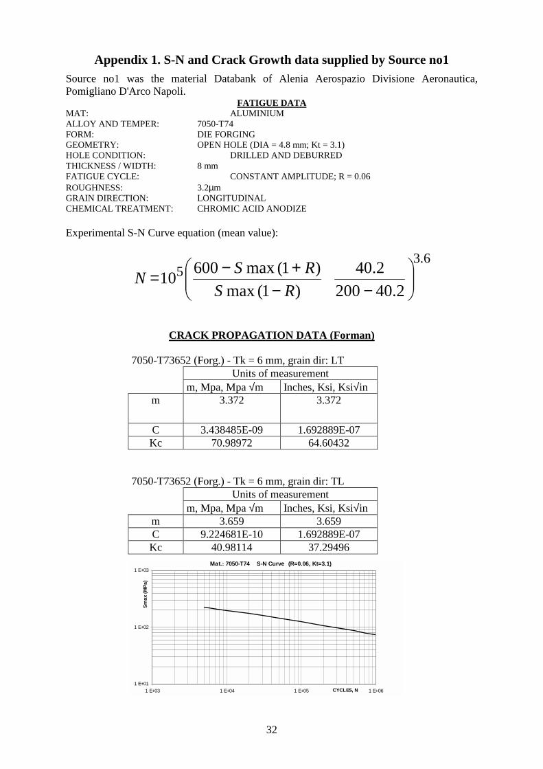
Figure 64. A typical da/DN final crack growth curve
Conclusions and Recommendations For Future Work. Stress-Life and crack growth calculations have been performed on the main frame panel shown in Figure 2. Various sensitivity studies have been performed which show the effect on fatigue life of, for instance, increased loading levels.
32
Appendix 1. S-N and Crack Growth data supplied by Source no1 Source no1 was the material Databank of Alenia Aerospazio Divisione Aeronautica, Pomigliano D'Arco Napoli.
FATIGUE DATA MAT: ALUMINIUM ALLOY AND TEMPER: 7050-T74 FORM: DIE FORGING GEOMETRY: OPEN HOLE (DIA = 4.8 mm; Kt = 3.1) HOLE CONDITION: DRILLED AND DEBURRED THICKNESS / WIDTH: 8 mm FATIGUE CYCLE: CONSTANT AMPLITUDE; R = 0.06 ROUGHNESS: 3.2µm GRAIN DIRECTION: LONGITUDINAL CHEMICAL TREATMENT: CHROMIC ACID ANODIZE Experimental S-N Curve equation (mean value):
CRACK PROPAGATION DATA (Forman) 7050-T73652 (Forg.) - Tk = 6 mm, grain dir: LT Units of measurement m, Mpa, Mpa √m Inches, Ksi, Ksi√in
m 3.372 3.372
C 3.438485E-09 1.692889E-07 Kc 70.98972 64.60432
7050-T73652 (Forg.) - Tk = 6 mm, grain dir: TL Units of measurement m, Mpa, Mpa √m Inches, Ksi, Ksi√in
m 3.659 3.659 C 9.224681E-10 1.692889E-07
Kc 40.98114 37.29496
Mat.: 7050-T74 S-N Curve (R=0.06, Kt=3.1)
1 E+01
1 E+02
1 E+03
1 E+03 1 E+04 1 E+05 1 E+06CYCLES, N
Smax
(MPa
)
6.35
2.402002.40
)1(max)1(max60010
−−
+−=RS
RSN
33
Appendix 2 Marc Results
Min Principal a=0
Min Principal a=1
Min Principal a=2
Min Principal a=3
Appendix 3 Nastran Results
Nastran a=0
Nastran a=1
Nastran a=2
Nastran a=3
34
Min Principal a=4
Min Principal a=5
Min Principal a=6
Min Principal a=7
Min Principal a=8
Nastran a=4
Nastran a=5
Nastran a=6
Nastran a=7
Nastran a=8
35
Appendix 4 Stress distribution across critical crack plane Plate in Figure 2 Plate in Figure 2 with hole removed
hole climb
hole cruise 1
hole fdapp1
no hole climb 1
no hole cruise 1
no hole fdapp1
36
hole flare
hole GT+15
hole init des 1
hole rotation
no hole flare
no hole GT+15
no hole init des 1
no hole rotation
37
hole taxi 07
hole TD1
hole unloaded
hole yaw1
no hole taxi 0.7
no hole TD1
no hole unloaded
no hole yaw 1