Embed Size (px)
Citation preview

8/20/2019 Stress Analysis INVENTOR
http://slidepdf.com/reader/full/stress-analysis-inventor 1/266
Contents
Chapter 1 Part Modal and Stress Analysis . . . . . . . . . . . . . . . . . . . 1
Simulation 1: About this tutorial . . . . . . . . . . . . . . . . . . . . . . 1Open the Model for Modal Analysis . . . . . . . . . . . . . . . . . . . . 3Enter the Stress Analysis Environment . . . . . . . . . . . . . . . . . . . 3Assign Material . . . . . . . . . . . . . . . . . . . . . . . . . . . . . . . 4Add Constraints . . . . . . . . . . . . . . . . . . . . . . . . . . . . . . 4Preview Mesh . . . . . . . . . . . . . . . . . . . . . . . . . . . . . . . . 6Run Simulation . . . . . . . . . . . . . . . . . . . . . . . . . . . . . . . 7
View the Results . . . . . . . . . . . . . . . . . . . . . . . . . . . . . . 7Summary . . . . . . . . . . . . . . . . . . . . . . . . . . . . . . . . . 11Simulation 2: About this tutorial . . . . . . . . . . . . . . . . . . . . . 12Copy Simulation . . . . . . . . . . . . . . . . . . . . . . . . . . . . . 13Create Parametric Geometry . . . . . . . . . . . . . . . . . . . . . . . 14Include Optimization Criteria . . . . . . . . . . . . . . . . . . . . . . . 16Add Loads . . . . . . . . . . . . . . . . . . . . . . . . . . . . . . . . . 16Set Convergence . . . . . . . . . . . . . . . . . . . . . . . . . . . . . . 17Run Simulation . . . . . . . . . . . . . . . . . . . . . . . . . . . . . . 18View the Results . . . . . . . . . . . . . . . . . . . . . . . . . . . . . . 19Summary . . . . . . . . . . . . . . . . . . . . . . . . . . . . . . . . . 21
Chapter 2 Assembly Stress Analysis . . . . . . . . . . . . . . . . . . . . . 23
About this tutorial . . . . . . . . . . . . . . . . . . . . . . . . . . . . . 23Get Started . . . . . . . . . . . . . . . . . . . . . . . . . . . . . . . . . 25
i

8/20/2019 Stress Analysis INVENTOR
http://slidepdf.com/reader/full/stress-analysis-inventor 2/266
Stress Analysis Environment . . . . . . . . . . . . . . . . . . . . . . . 25Excluding Components . . . . . . . . . . . . . . . . . . . . . . . . . . 26
Assign Materials . . . . . . . . . . . . . . . . . . . . . . . . . . . . . . 27Add Constraints and Loads . . . . . . . . . . . . . . . . . . . . . . . . 28Stress Analysis Settings . . . . . . . . . . . . . . . . . . . . . . . . . . 31Contact Conditions . . . . . . . . . . . . . . . . . . . . . . . . . . . . 32Generate Meshes . . . . . . . . . . . . . . . . . . . . . . . . . . . . . 33Run the Simulation . . . . . . . . . . . . . . . . . . . . . . . . . . . . 34View and Interpret the Results . . . . . . . . . . . . . . . . . . . . . . 35Summary . . . . . . . . . . . . . . . . . . . . . . . . . . . . . . . . . 37
Chapter 3 Contacts and Mesh Refinement . . . . . . . . . . . . . . . . . 39
About this tutorial . . . . . . . . . . . . . . . . . . . . . . . . . . . . . 39Open the Model . . . . . . . . . . . . . . . . . . . . . . . . . . . . . . 40Stress Analysis Environment . . . . . . . . . . . . . . . . . . . . . . . 41Create a Simulation . . . . . . . . . . . . . . . . . . . . . . . . . . . . 41Exclude Components . . . . . . . . . . . . . . . . . . . . . . . . . . . 42Assign Materials . . . . . . . . . . . . . . . . . . . . . . . . . . . . . . 42Add Constraints and Loads . . . . . . . . . . . . . . . . . . . . . . . . 43Define Contact Conditions . . . . . . . . . . . . . . . . . . . . . . . . 46Specify and Preview Meshes . . . . . . . . . . . . . . . . . . . . . . . . 50Run the Simulation . . . . . . . . . . . . . . . . . . . . . . . . . . . . 51View and Interpret the Results . . . . . . . . . . . . . . . . . . . . . . 51Copy and Modify Simulation . . . . . . . . . . . . . . . . . . . . . . . 54Specify Local Mesh Controls . . . . . . . . . . . . . . . . . . . . . . . 54Run the Simulation Again . . . . . . . . . . . . . . . . . . . . . . . . . 56View and Interpret the Results Again . . . . . . . . . . . . . . . . . . . 57Summary . . . . . . . . . . . . . . . . . . . . . . . . . . . . . . . . . 59
Chapter 4 Assembly Modal Analysis . . . . . . . . . . . . . . . . . . . . . 61About this tutorial . . . . . . . . . . . . . . . . . . . . . . . . . . . . . 62Open the Assembly . . . . . . . . . . . . . . . . . . . . . . . . . . . . 64Create a Simulation Study . . . . . . . . . . . . . . . . . . . . . . . . . 65Exclude Components . . . . . . . . . . . . . . . . . . . . . . . . . . . 66Assign Materials . . . . . . . . . . . . . . . . . . . . . . . . . . . . . . 67Add Constraints . . . . . . . . . . . . . . . . . . . . . . . . . . . . . . 67Create Manual Contacts . . . . . . . . . . . . . . . . . . . . . . . . . . 68Specify Mesh Options . . . . . . . . . . . . . . . . . . . . . . . . . . . 70Preview Mesh and Run Simulation . . . . . . . . . . . . . . . . . . . . 70View and Interpret Results . . . . . . . . . . . . . . . . . . . . . . . . 71Summary . . . . . . . . . . . . . . . . . . . . . . . . . . . . . . . . . 73
Chapter 5 FEA Assembly Optimization . . . . . . . . . . . . . . . . . . . . 75
About this tutorial . . . . . . . . . . . . . . . . . . . . . . . . . . . . . 76
ii | Contents

8/20/2019 Stress Analysis INVENTOR
http://slidepdf.com/reader/full/stress-analysis-inventor 3/266
Open the Assembly . . . . . . . . . . . . . . . . . . . . . . . . . . . . 77Define the Simulation . . . . . . . . . . . . . . . . . . . . . . . . . . . 77
Assign Materials . . . . . . . . . . . . . . . . . . . . . . . . . . . . . . 78Adding Constraints . . . . . . . . . . . . . . . . . . . . . . . . . . . . 78Adding Loads . . . . . . . . . . . . . . . . . . . . . . . . . . . . . . . 79Modify the Mesh . . . . . . . . . . . . . . . . . . . . . . . . . . . . . 80Preview the Mesh . . . . . . . . . . . . . . . . . . . . . . . . . . . . . 81Create Parametric Geometry . . . . . . . . . . . . . . . . . . . . . . . 82Optimization Criteria . . . . . . . . . . . . . . . . . . . . . . . . . . . 84Run the Simulation . . . . . . . . . . . . . . . . . . . . . . . . . . . . 85View and Interpret the Results . . . . . . . . . . . . . . . . . . . . . . 85View and animate 3D plots . . . . . . . . . . . . . . . . . . . . . . . . 87View XY Plots . . . . . . . . . . . . . . . . . . . . . . . . . . . . . . . 88Summary . . . . . . . . . . . . . . . . . . . . . . . . . . . . . . . . . 90
Chapter 6 Stress Analysis Contacts . . . . . . . . . . . . . . . . . . . . . . 93
About this tutorial . . . . . . . . . . . . . . . . . . . . . . . . . . . . . 93Overview . . . . . . . . . . . . . . . . . . . . . . . . . . . . . . . . . 94Open the Assembly . . . . . . . . . . . . . . . . . . . . . . . . . . . . 94How a Caulk Gun Works . . . . . . . . . . . . . . . . . . . . . . . . . 96Assembly Simulation . . . . . . . . . . . . . . . . . . . . . . . . . . . 99Contact Types . . . . . . . . . . . . . . . . . . . . . . . . . . . . . . 100Bonded Contact . . . . . . . . . . . . . . . . . . . . . . . . . . . . . 102Separation Contact . . . . . . . . . . . . . . . . . . . . . . . . . . . . 103Sliding and No Separation Contact . . . . . . . . . . . . . . . . . . . 104Separation and No Sliding Contact . . . . . . . . . . . . . . . . . . . 107Shrink Fit and No Sliding Contact . . . . . . . . . . . . . . . . . . . . 108Spring Contact . . . . . . . . . . . . . . . . . . . . . . . . . . . . . . 110Loads and Constraints . . . . . . . . . . . . . . . . . . . . . . . . . . 111Simulation Results . . . . . . . . . . . . . . . . . . . . . . . . . . . . 112
Summary . . . . . . . . . . . . . . . . . . . . . . . . . . . . . . . . . 114
Chapter 7 Frame Analysis . . . . . . . . . . . . . . . . . . . . . . . . . . 117
About this tutorial . . . . . . . . . . . . . . . . . . . . . . . . . . . . 117Open the Assembly . . . . . . . . . . . . . . . . . . . . . . . . . . . 119Frame Analysis Environment . . . . . . . . . . . . . . . . . . . . . . 119Frame Analysis Settings . . . . . . . . . . . . . . . . . . . . . . . . . 122Assign Materials . . . . . . . . . . . . . . . . . . . . . . . . . . . . . 122Change Beam Properties . . . . . . . . . . . . . . . . . . . . . . . . . 124Change Direction of Gravity . . . . . . . . . . . . . . . . . . . . . . . 124Add Constraints . . . . . . . . . . . . . . . . . . . . . . . . . . . . . 125Add Constraints to the Next Beam . . . . . . . . . . . . . . . . . . . 128Add Loads . . . . . . . . . . . . . . . . . . . . . . . . . . . . . . . . 129
Run the Simulation . . . . . . . . . . . . . . . . . . . . . . . . . . . 131View and Interpret Results . . . . . . . . . . . . . . . . . . . . . . . . 132
Contents | iii

8/20/2019 Stress Analysis INVENTOR
http://slidepdf.com/reader/full/stress-analysis-inventor 4/266
Summary . . . . . . . . . . . . . . . . . . . . . . . . . . . . . . . . . 133
Chapter 8 Frame Analysis Results . . . . . . . . . . . . . . . . . . . . . . 135
About this tutorial . . . . . . . . . . . . . . . . . . . . . . . . . . . . 135Get Started . . . . . . . . . . . . . . . . . . . . . . . . . . . . . . . . 136Frame Analysis Environment . . . . . . . . . . . . . . . . . . . . . . 137View and Interpret the Results . . . . . . . . . . . . . . . . . . . . . . 139Display Maximum and Minimum Values . . . . . . . . . . . . . . . . 140View Beam Detail . . . . . . . . . . . . . . . . . . . . . . . . . . . . 141Display and Edit Diagrams . . . . . . . . . . . . . . . . . . . . . . . . 142Adjust Displacement Display . . . . . . . . . . . . . . . . . . . . . . 144Animate the Results . . . . . . . . . . . . . . . . . . . . . . . . . . . 146Generate Report . . . . . . . . . . . . . . . . . . . . . . . . . . . . . 147Summary . . . . . . . . . . . . . . . . . . . . . . . . . . . . . . . . . 148
Chapter 9 Frame Analysis Connections . . . . . . . . . . . . . . . . . . . 149About this tutorial . . . . . . . . . . . . . . . . . . . . . . . . . . . . 149Connections Overview . . . . . . . . . . . . . . . . . . . . . . . . . . 150Open the Assembly . . . . . . . . . . . . . . . . . . . . . . . . . . . 151Frame Analysis Environment . . . . . . . . . . . . . . . . . . . . . . 152Change Direction of Gravity . . . . . . . . . . . . . . . . . . . . . . . 154Add Custom Nodes . . . . . . . . . . . . . . . . . . . . . . . . . . . 154Add Custom Nodes . . . . . . . . . . . . . . . . . . . . . . . . . . . 157Change Color of Custom Nodes . . . . . . . . . . . . . . . . . . . . . 159Assign Rigid Links . . . . . . . . . . . . . . . . . . . . . . . . . . . . 160Add Constraints . . . . . . . . . . . . . . . . . . . . . . . . . . . . . 164Run the Simulation . . . . . . . . . . . . . . . . . . . . . . . . . . . 165View the Results . . . . . . . . . . . . . . . . . . . . . . . . . . . . . 166Assign a Release . . . . . . . . . . . . . . . . . . . . . . . . . . . . . 167
Run the Simulation Again . . . . . . . . . . . . . . . . . . . . . . . . 169View the Updated Results . . . . . . . . . . . . . . . . . . . . . . . . 170Summary . . . . . . . . . . . . . . . . . . . . . . . . . . . . . . . . . 171
Chapter 10 Modal Type of Frame Analysis . . . . . . . . . . . . . . . . . . 173
About this tutorial . . . . . . . . . . . . . . . . . . . . . . . . . . . . 173Open the Assembly . . . . . . . . . . . . . . . . . . . . . . . . . . . 175Frame Analysis Environment . . . . . . . . . . . . . . . . . . . . . . 175Create a Simulation Study . . . . . . . . . . . . . . . . . . . . . . . . 175Run the Simulation . . . . . . . . . . . . . . . . . . . . . . . . . . . 176View the Results . . . . . . . . . . . . . . . . . . . . . . . . . . . . . 177Animate the Results . . . . . . . . . . . . . . . . . . . . . . . . . . . 178Summary . . . . . . . . . . . . . . . . . . . . . . . . . . . . . . . . . 179
Chapter 11 Dynamic Simulation - Part 1 . . . . . . . . . . . . . . . . . . . 181
iv | Contents

8/20/2019 Stress Analysis INVENTOR
http://slidepdf.com/reader/full/stress-analysis-inventor 5/266
About this tutorial . . . . . . . . . . . . . . . . . . . . . . . . . . . . 181Open the Assembly . . . . . . . . . . . . . . . . . . . . . . . . . . . 182
Degrees of Freedom . . . . . . . . . . . . . . . . . . . . . . . . . . . 183Automatic Constraint Conversion . . . . . . . . . . . . . . . . . . . . 184Assembly Constraints . . . . . . . . . . . . . . . . . . . . . . . . . . 187Add a Rolling Joint . . . . . . . . . . . . . . . . . . . . . . . . . . . . 189Building a 2D Contact . . . . . . . . . . . . . . . . . . . . . . . . . . 190Add Spring, Damper, and Jack Joint . . . . . . . . . . . . . . . . . . . 193Define Gravity . . . . . . . . . . . . . . . . . . . . . . . . . . . . . . 195Impose Motion on a Joint . . . . . . . . . . . . . . . . . . . . . . . . 196Run a Simulation . . . . . . . . . . . . . . . . . . . . . . . . . . . . . 197Using the Output Grapher . . . . . . . . . . . . . . . . . . . . . . . . 198Simulation Player . . . . . . . . . . . . . . . . . . . . . . . . . . . . 199Summary . . . . . . . . . . . . . . . . . . . . . . . . . . . . . . . . . 202
Chapter 12 Dynamic Simulation - Part 2 . . . . . . . . . . . . . . . . . . . 205
About this tutorial . . . . . . . . . . . . . . . . . . . . . . . . . . . . 205Work in the Simulation Environment . . . . . . . . . . . . . . . . . . 206Construct the Operating Conditions . . . . . . . . . . . . . . . . . . 208Add Friction . . . . . . . . . . . . . . . . . . . . . . . . . . . . . . . 210Add a Sliding Joint . . . . . . . . . . . . . . . . . . . . . . . . . . . . 212Use the Input Grapher . . . . . . . . . . . . . . . . . . . . . . . . . . 213Use the Output Grapher . . . . . . . . . . . . . . . . . . . . . . . . . 217Export to FEA . . . . . . . . . . . . . . . . . . . . . . . . . . . . . . . 219Publish Output in Inventor Studio . . . . . . . . . . . . . . . . . . . 223Summary . . . . . . . . . . . . . . . . . . . . . . . . . . . . . . . . . 225
Chapter 13 Assembly Motion and Loads . . . . . . . . . . . . . . . . . . . 227
About this tutorial . . . . . . . . . . . . . . . . . . . . . . . . . . . . 227
Open Assembly . . . . . . . . . . . . . . . . . . . . . . . . . . . . . . 229Activate Dynamic Simulation . . . . . . . . . . . . . . . . . . . . . . 231Automatic Joint Creation . . . . . . . . . . . . . . . . . . . . . . . . 231Define Gravity . . . . . . . . . . . . . . . . . . . . . . . . . . . . . . 232Insert a Spring . . . . . . . . . . . . . . . . . . . . . . . . . . . . . . 232Define the Spring Properties . . . . . . . . . . . . . . . . . . . . . . . 235Run the Simulation . . . . . . . . . . . . . . . . . . . . . . . . . . . 236Insert a Contact Joint . . . . . . . . . . . . . . . . . . . . . . . . . . 237Edit the Joint Properties . . . . . . . . . . . . . . . . . . . . . . . . . 239Add Imposed Motion . . . . . . . . . . . . . . . . . . . . . . . . . . 241View the Simulation Results . . . . . . . . . . . . . . . . . . . . . . . 241View the Simulation Results (continued) . . . . . . . . . . . . . . . . 242Export the Data . . . . . . . . . . . . . . . . . . . . . . . . . . . . . 243Summary . . . . . . . . . . . . . . . . . . . . . . . . . . . . . . . . . 244
Contents | v

8/20/2019 Stress Analysis INVENTOR
http://slidepdf.com/reader/full/stress-analysis-inventor 6/266
Chapter 14 FEA using Motion Loads . . . . . . . . . . . . . . . . . . . . . 245
About this tutorial . . . . . . . . . . . . . . . . . . . . . . . . . . . . 246Open Assembly File . . . . . . . . . . . . . . . . . . . . . . . . . . . 247Run a Simulation . . . . . . . . . . . . . . . . . . . . . . . . . . . . . 249Generate Time Steps . . . . . . . . . . . . . . . . . . . . . . . . . . . 249Export to Stress Analysis . . . . . . . . . . . . . . . . . . . . . . . . . 249Use the Motion Loads in Stress Analysis . . . . . . . . . . . . . . . . . 253Generate a report . . . . . . . . . . . . . . . . . . . . . . . . . . . . . 256Summary . . . . . . . . . . . . . . . . . . . . . . . . . . . . . . . . . 257
Index . . . . . . . . . . . . . . . . . . . . . . . . . . . . . . . 259
vi | Contents

8/20/2019 Stress Analysis INVENTOR
http://slidepdf.com/reader/full/stress-analysis-inventor 7/266
Part Modal and StressAnalysis
Simulation 1: About this tutorial
Modal analysis.
SimulationCategory
20 minutesTime Required
1
1

8/20/2019 Stress Analysis INVENTOR
http://slidepdf.com/reader/full/stress-analysis-inventor 8/266
PivotBracket.iptTutorial Files
Used
You will create two simulations: modal analysis of the part and a parametric
structural static analysis on the same part.
The Modal Analysis tutorial walks through the process of defining and
performing a structural frequency analysis, or modal analysis, for a part. The
simulation generates the natural frequencies (Eigenvalues) and corresponding
mode shapes which we view and interpret at the end of the tutorial.
The second simulation is a parametric study on the same model. Parametric
studies vary the design parameters to update geometry and evaluate various
configurations for a design case. We perform a structural static analysis with
the goal of minimizing model weight.
Objectives
■ Create a simulation for modal analysis
■ Override the model material with a different material
■ Specify constraints
■ Run the simulation
■ View and interpret the results
Prerequisites
■ Familiarity with the ribbon user interface and Quick Access Toolbar.
■ Familiarity with the use of the model browser and context menus.
■
See the Help topic“Getting Started
” for further information.
Navigation Tips
■ Use Show in the upper-left corner to display the table of contents for this
tutorial with navigation links to each page.
■ Use Forward in the upper-right corner to advance to the next page.
Next (page 3)
2 | Chapter 1 Part Modal and Stress Analysis

8/20/2019 Stress Analysis INVENTOR
http://slidepdf.com/reader/full/stress-analysis-inventor 9/266
Open the Model for Modal Analysis
Let’s get started on the Modal Analysis simulation first.
1 On the Quick Access Toolbar, click the Open command.
2 Set your project file to Tutorial_Files.ipj if not already set.
3 Select the part model named PivotBracket.ipt.
4 Click Open.
Previous (page 1) | Next (page 3)
Enter the Stress Analysis Environment
The stress analysis environment is one of a handful of Inventor environments
that enable specialized activity relative to the model. In this case, it
incorporates commands for doing part and assembly stress analysis.
To enter the stress analysis environment and start a simulation:
1 Click the Environments tab in the ribbon bar. The list of available
environments is presented.
2 Click the Stress Analysis environment command.
3 Click Create Simulation.
4 The Create New Simulation dialog box displays. Specify the name Modal
Analysis.
5 In the Simulation Type tab, select Modal Analysis.
6 Leave the remaining settings in their current state and click OK. A new
simulation is started and the browser is populated with stress
analysis-related folders.
Previous (page 3) | Next (page 4)
Open the Model for Modal Analysis | 3
8/20/2019 Stress Analysis INVENTOR
http://slidepdf.com/reader/full/stress-analysis-inventor 10/266
Assign Material
For any component that you want to analyze, check the material to make sure
that it is defined. Some Inventor materials do not have “simulation-ready”
properties and need modification before using them in simulations. If you
use an inadequately defined material, a message displays. Modify the material
or select another material.
You can use different materials in different simulations and compare the
results in a report. To assign a different material:
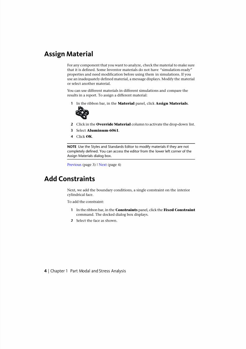
1 In the ribbon bar, in the Material panel, click Assign Materials.
2 Click in the Override Material column to activate the drop-down list.
3 Select Aluminum-6061.
4 Click OK.
NOTE Use the Styles and Standards Editor to modify materials if they are not
completely defined. You can access the editor from the lower left corner of the
Assign Materials dialog box.
Previous (page 3) | Next (page 4)
Add Constraints
Next, we add the boundary conditions, a single constraint on the interior
cylindrical face.
To add the constraint:
1 In the ribbon bar, in the Constraints panel, click the Fixed Constraint
command. The docked dialog box displays.
2 Select the face as shown.
4 | Chapter 1 Part Modal and Stress Analysis

8/20/2019 Stress Analysis INVENTOR
http://slidepdf.com/reader/full/stress-analysis-inventor 11/266
3 Click OK.
The model is now constrained by that face. The browser constraints folder is
populated with a node representing the constraint.
Previous (page 4) | Next (page 6)
Add Constraints | 5
8/20/2019 Stress Analysis INVENTOR
http://slidepdf.com/reader/full/stress-analysis-inventor 12/266
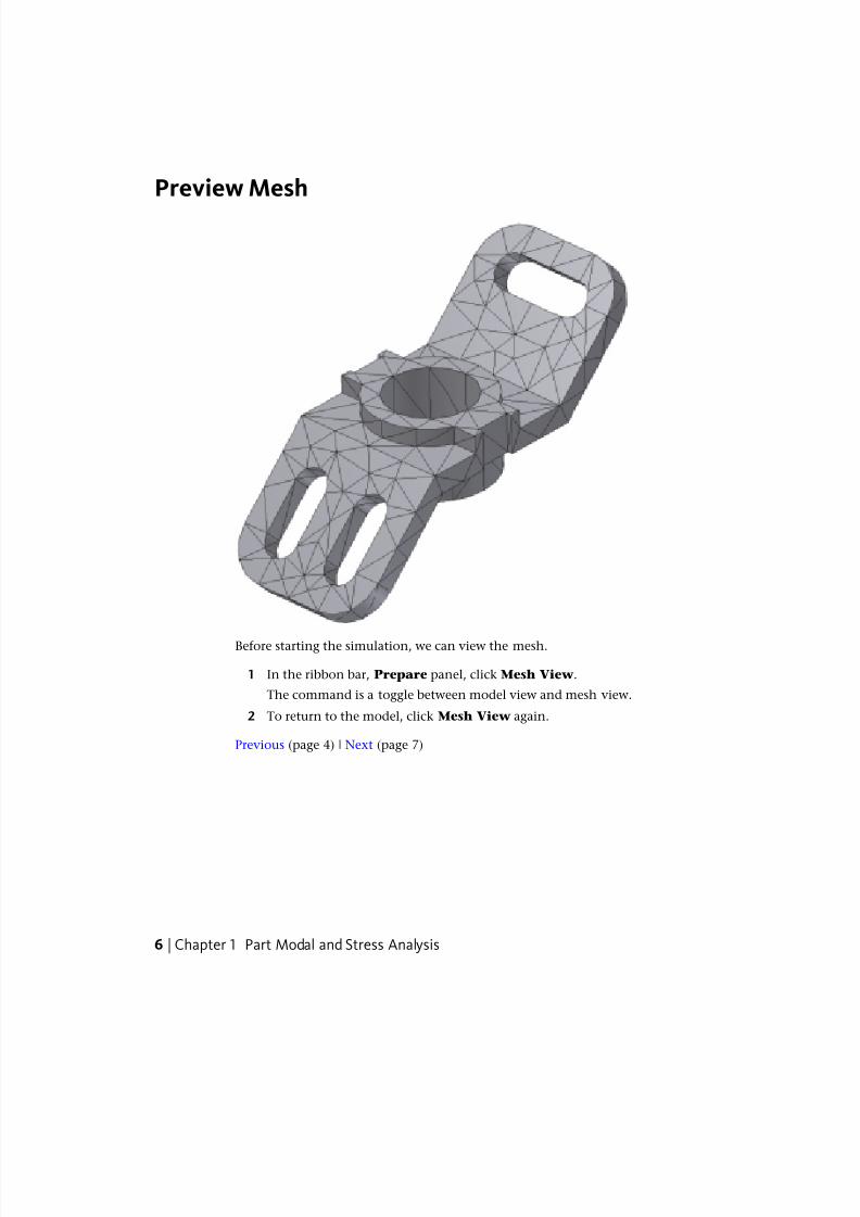
Preview Mesh
Before starting the simulation, we can view the mesh.
1 In the ribbon bar, Prepare panel, click Mesh View.
The command is a toggle between model view and mesh view.
2 To return to the model, click Mesh View again.
Previous (page 4) | Next (page 7)
6 | Chapter 1 Part Modal and Stress Analysis
8/20/2019 Stress Analysis INVENTOR
http://slidepdf.com/reader/full/stress-analysis-inventor 13/266
Run Simulation
Now, to run the simulation.
1 In the Solve panel, click the Simulate command to display the Simulate
dialog box.
2 Check the More section of the dialog box for messages. Click Run to
display the simulation progress. Wait for the simulation to finish.
Previous (page 6) | Next (page 7)
View the Results
After the simulation finishes, the Results folder populates with the variousresults types. The graphics region displays the first mode shaded plot.
In the browser under the Results node and then the Modal Frequency
node, notice the first mode shape (F1) has a check mark by it, indicating it is
being displayed. There are nodes for the mode shapes corresponding to each
natural frequency. The color chart shows relative displacement values. The
units are not applicable since the mode shapes values are relative. (They have
no actual physical value at this point.)
Now you can perform post-processing tasks using the Display commands
located on the ribbon bar. The commands are described in Help.
Run Simulation | 7

8/20/2019 Stress Analysis INVENTOR
http://slidepdf.com/reader/full/stress-analysis-inventor 14/266
For post-processing of structural frequency simulation studies, the browser
list shows the natural frequencies. Double-click any of these nodes to show
the corresponding Mode Shape 3D plot.
1 Animate the results using the Animate Results command in the Result
panel on the ribbon bar.
2 While the animation is playing, click Orbit in the navigation tools on
the side of the graphics window. As you orbit the graphics, the animation
continues to play.
NOTE The following image depicts a frame from the animation of modeF3.
8 | Chapter 1 Part Modal and Stress Analysis

8/20/2019 Stress Analysis INVENTOR
http://slidepdf.com/reader/full/stress-analysis-inventor 15/266
3 Click OK.
4 In the Results browser list of natural frequencies, double-click the results
for mode F3 to display that mode.
View the Results | 9

8/20/2019 Stress Analysis INVENTOR
http://slidepdf.com/reader/full/stress-analysis-inventor 16/266
10 | Chapter 1 Part Modal and Stress Analysis

8/20/2019 Stress Analysis INVENTOR
http://slidepdf.com/reader/full/stress-analysis-inventor 17/266
NOTE If you plan to complete the second part of this tutorial, keep this model file
open. Otherwise, save your model file to a different name before you close it.
Previous (page 7) | Next (page 11)
Summary
In this first tutorial for Part Stress Analysis, you learned how to:
■ Create a simulation for modal analysis.
■ Override the model material with a different material.
■ Specify constraints.
■ Run the simulation.
■ View and interpret the results.
What Next? Continue with “Simulation 2 - Parametric Static Analysis”
Previous (page 7) | Next (page 12)
Summary | 11

8/20/2019 Stress Analysis INVENTOR
http://slidepdf.com/reader/full/stress-analysis-inventor 18/266
Simulation 2: About this tutorial
12 | Chapter 1 Part Modal and Stress Analysis

8/20/2019 Stress Analysis INVENTOR
http://slidepdf.com/reader/full/stress-analysis-inventor 19/266
Parametric static analysis.
Level 3 special interestSkill Level
20 minutesTime Required
PivotBracket.iptTutorial Files
Used
The second simulation is a parametric study on the same model. Parametric
studies vary the parameters of the model to update geometry and evaluate
various configurations of a design. In this structural static analysis, the goal
is to minimize the weight of the model.
Objectives
■ Copy a simulation.
■ Use analysis parameters to evaluate how to refine the weight of the model.
■ Generate configurations of the parametric dimension geometry.
■ Modify design constraints and view results based on those changes.
Prerequisites
■ Completed Simulation 1 (Modal Analysis), the first part of this tutorial set.
■ See the Help topic “Getting Started” for further information.
Navigation Tips
■ Use Show in the upper-left corner to display the table of contents for this
tutorial with navigation links to each page.
■ Use Forward in the upper-right corner to advance to the next page.
Previous (page 11) | Next (page 13)
Copy Simulation
We will create a copy of the first simulation, and edit it to define the second
analysis.
1 In the browser, right-click the Simulation (Modal Analysis) node
and click Copy Simulation. A copy of this simulation is added to the
browser and becomes the active simulation.
Copy Simulation | 13

8/20/2019 Stress Analysis INVENTOR
http://slidepdf.com/reader/full/stress-analysis-inventor 20/266
We will edit the simulation properties to define a parametric dimension
study.
2 Right-click the newly created Simulation node, and click Edit
Simulation Properties.
3 Change the name to Parametric.
4 Change the Design Objective to Parametric Dimension using the
drop-down list.
5 Set the simulation type to Static Analysis.
6 Click OK.
Previous (page 12) | Next (page 14)
Create Parametric GeometryWe will produce a range of geometric configurations involving the thickness
of the model to facilitate weight optimization. Adding parameters to the
parametric table is required.
Add parameters to the parametric table
1 In the Manage panel, click Parametric Table.
2 In the browser, right-click the part node just below the Simulation
(Parametric) node, and click Show Parameters.
3 In the Select Parameters dialog box, check the box to the left of the
parameter named d2, 12 mm.
4 Click OK.
After identifying the parameter we want to use, we must define a range for
the parameter and generate the corresponding geometric configurations.
Define parameter range
1 In the Values cell for Extrusion1 d2, enter the range 6-12. The values
must be in ascending order.
2 Press Enter to accept the values. When you click inside the Value field,
the value now says 6-12:3. This indicates that there are now three values
in the range. These are equally divided between the first and last number,
hence that values are 6, 9, and 12.
14 | Chapter 1 Part Modal and Stress Analysis

8/20/2019 Stress Analysis INVENTOR
http://slidepdf.com/reader/full/stress-analysis-inventor 21/266
NOTE The number after the colon specifies the additional configurations
desired, excluding the base configuration. The base is 12 mm, and the two
additional configurations are 6 mm and 9 mm.
Once the parameter range is specified, we can generate the various
configurations based on the range values.
Generate configurations
1 Right-click the table parameter row, and select Generate All
Configurations. The model generation process is started.
2 After the model regeneration is completed, move the slider to see the
different shapes created.
Create Parametric Geometry | 15

8/20/2019 Stress Analysis INVENTOR
http://slidepdf.com/reader/full/stress-analysis-inventor 22/266
We are not finished with the Parametric Table yet, so do not close it.
Previous (page 13) | Next (page 16)
Include Optimization Criteria
Remember that our goal for this simulation is to minimize weight. We optimize
the simulation using a range of geometric configurations generated previously
while utilizing the Yield Strength failure criteria.
Add Design Constraints
1 In the Design Constraints section, pause the cursor over the empty
row, right-click, and click Add Design Constraint.
2 In the Select Design Constraint dialog box, click Mass, and click OK.3 Repeat step 1.
4 In the Select Design Constraint dialog box, Select Von Mises Stress.
Ensure that Geometry Selections is All Geometry.
5 Click OK.
Enter Limit values and safety factor
1 In the Von Mises Stress row, click in the Constraint type cell, and
select Upper Limit from the drop-down list.
2 Enter 20 for Limit.
3 Enter 1.5 for Safety Factor .
Previous (page 14) | Next (page 16)
Add Loads
Next, add the structural load.
1 Click the Force Load command. The dialog box displays.
2 Select the face as shown.
16 | Chapter 1 Part Modal and Stress Analysis

8/20/2019 Stress Analysis INVENTOR
http://slidepdf.com/reader/full/stress-analysis-inventor 23/266
3 Enter 200 N for the Magnitude.
4 Click OK.
Previous (page 16) | Next (page 17)
Set Convergence
The software performs an automatic H-P refinement for parts. In this case, wewant to add an additional H refinement iteration. H refinement increases the
number of mesh elements in areas where the results need improvement. The
P refinement increases the polynomial degree of the selected elements in the
high stress areas to improve the accuracy of the results.
1 In the Prepare panel, click Convergence Settings.
2 For Maximum Number of h Refinements, enter 1.
3 Click OK.
Previous (page 16) | Next (page 18)
Set Convergence | 17

8/20/2019 Stress Analysis INVENTOR
http://slidepdf.com/reader/full/stress-analysis-inventor 24/266
Run Simulation
Now we will run the simulation. To start the Simulation, use the Simulate
command in the ribbon bar or through the simulation node context menu.
1 Click the Simulate command to display the Simulate dialog box.
2 Click Run. The Simulation progress displays. Wait for the simulation
to finish.
When the simulation is complete, the Von Mises Stress plot displays by
default.
3 In the Display panel, click Adjust Displacement Display ,
drop-down list, and select Actual.
Previous (page 17) | Next (page 19)
18 | Chapter 1 Part Modal and Stress Analysis

8/20/2019 Stress Analysis INVENTOR
http://slidepdf.com/reader/full/stress-analysis-inventor 25/266
View the Results
After the simulation finishes, the graphics region displays a 3D color plot, and
you can see that the Result folder is populated. Now we can evaluate the
results through the parametric table and the 3D and XY plots available for
post processing.
Optimize model
First, we optimize the mass using the parametric table populated in previous
steps. Then we look at 3D and XY plots to understand the behavior of the
model under the defined boundary conditions.
The goal is to minimize the mass of the model taking into account parametric
dimensions and stress constraints.
1 If you previously closed the Parametric table, reopen it by clicking theParametric Table command.
2 For the Mass Design Constraint, click in the Constraint Type cell,
and select Minimize from the drop-down list.
The parametric values change to show the configuration with the least mass
that meets the given constraints. In this case, the original thickness value was
12 mm and the optimized value is 9 mm which in turn reduces the mass of
the model.
Note the design constraint Result Value for Max Von Mises Stress. The
value has a green circle preceding it. It indicates that the design constraint
value is within the safety factor range.
Slide the Extrusion1 parameter value to 6. When the table updates, you willsee that the design constraint Result Value is now outside the safety factor.
The value is preceded by a red square indicating the design constraint value
has been exceeded the safety factor. Slide the parameter value back to 9.
View and animate 3D plots
Now you can perform post-processing tasks using the Display panel commands
for smooth shading, contour plots, etc. These commands are described in
Help.
1 In the Result panel, click Animate Results.
2 In the Animate dialog box, click the Play command. The Von
Mises Stress plot colors change to reflect the application of the load. To
View the Results | 19

8/20/2019 Stress Analysis INVENTOR
http://slidepdf.com/reader/full/stress-analysis-inventor 26/266
view the deformation changes, stop the animation, select Adjusted x1
from the Adjust Displacement Display , drop-down list andrestart the animation.
For post-processing of results, double-click the result in the browser to display
the result in the graphics region. Then, select the Display command you want
to use.
View XY graphs
XY Charts show a result component over the range of a parameter.
To view an XY plot, right-click over the parameter row in the Parametric Table
and choose XY Plot.
In this case, the above XY plot displays Stress results versus parametric
configurations.
Previous (page 18) | Next (page 21)
20 | Chapter 1 Part Modal and Stress Analysis

8/20/2019 Stress Analysis INVENTOR
http://slidepdf.com/reader/full/stress-analysis-inventor 27/266
Summary
In this last tutorial for Part Stress Analysis, you learned how to:
■ Copy a simulation.
■ Modify the simulation properties to change the type of simulation.
■ Generate configurations of the parametric dimension geometry.
■ Use analysis parameters to evaluate how to refine the weight of the model.
■ Modify design constraints and view results based on those changes.
What Next? As a next step, consider doing the Assembly FEA tutorials. If
you have already completed them, why not acquaint yourself with the
Dynamic Simulation tutorials?
Experiment with what you have seen and used. Explore how you can use this
design tool to help you complete your digital prototype with confidence in
its performance.
Previous (page 19)
Summary | 21

8/20/2019 Stress Analysis INVENTOR
http://slidepdf.com/reader/full/stress-analysis-inventor 28/266
22

8/20/2019 Stress Analysis INVENTOR
http://slidepdf.com/reader/full/stress-analysis-inventor 29/266
Assembly Stress Analysis
About this tutorial
Simulate the structural static behavior of an assembly for analysis.
SimulationCategory
35 minutesTime Required
2
23
8/20/2019 Stress Analysis INVENTOR
http://slidepdf.com/reader/full/stress-analysis-inventor 30/266
analyze-2.iamTutorial File Used
NOTE Click and read the required Tutorial Files Installation Instructions atht-
tp://www.autodesk.com/inventor-tutorial-data-sets . Then download the tutorial
data sets and the required Tutorial Files Installation Instructions, and install the
datasets as instructed.
The stress analysis environment is a special environment within assembly,
part, sheet metal, and weldment documents. The environment has commands
unique to its purpose.
We analyze a subset of an assembly using the “exclude from simulation”
functionality in Stress Analysis. Contact types are changed as required by the
physical behavior of the model. Meshing settings are adjusted to capture the
geometry of the model more accurately.
Objectives
■ Create a simulation.
■ Evaluate and assign materials as needed.
■ Add loads and constraints.
■ Identify contact conditions.
■ Create a mesh.
■ Run a simulation.
■ View and interpret the results.
Prerequisites
■ Know how to use the Quick Access toolbar, tabs and panels on the ribbon,model browser, and context menus.
■ Know how to navigate the model space with the various view tools.
■ Know how to specify and edit project files.
■ See the Help topic “Getting Started” for further information.
Navigation Tips
■ Use Next or Previous at the bottom-left to advance to the next page or
return to the previous one.
Next (page 25)
24 | Chapter 2 Assembly Stress Analysis

8/20/2019 Stress Analysis INVENTOR
http://slidepdf.com/reader/full/stress-analysis-inventor 31/266
Get Started
To begin with, we will open the assembly to analyze. With Autodesk Inventor
up and running, but with no model open, do the following:
1 Click the Open command on the Quick Access toolbar.
2 Set the Project File to Tutorial_Files.ipj
3 Select Assembly FEA 1
➤
analyze-2.iam.
4 Click Open.
5 Save the file with a different name, such as: analyze-2_tutorial.iam
Previous (page 23) | Next (page 25)
Stress Analysis Environment
We are ready to enter the stress analysis environment.
1 On the ribbon, click Environments tab
➤
Begin panel ➤
Stress
Analysis .
2 On the Manage panel, click the Create Simulation command.
The Create New Simulation dialog box displays.
The settings provide opportunity to tailor the simulation by specifying
a unique name, single point or parametric dimension design objective,
and other parameters.
NOTE On the Model State tab, you specify the Design View,
Positional, and Level of Detail to use for the simulation. The settings
can be different for each simulation.
3 Click OK to accept the default settings for this simulation.
The browser populates with a hierarchical structure of the assembly and
analysis-related folders.
Most of the commands in the ribbon panels are now enabled for use. Disabledcommands enable as their use criteria is satisfied.
Get Started | 25
8/20/2019 Stress Analysis INVENTOR
http://slidepdf.com/reader/full/stress-analysis-inventor 32/266
Previous (page 25) | Next (page 26)
Excluding Components
You can exclude components that are not affected by the simulation or whose
function is simulated by constraints or forces.
We will exclude the following parts from this simulation:
■ Handle
■ Screw
■ SHCS_10-32x6
To exclude these components:
1 Expand the analyze-2_tutorial.iam browser node.
2 Right-click Handle, and click Exclude From Simulation.
3 Repeat the command for both the Screw and SHCS_10-32x6
components.
The default display setting for excluded components is partially transparent
as seen in the following image:
26 | Chapter 2 Assembly Stress Analysis

8/20/2019 Stress Analysis INVENTOR
http://slidepdf.com/reader/full/stress-analysis-inventor 33/266
Previous (page 25) | Next (page 27)
Assign Materials
The next step is to look at the component materials and make adjustments.
For this simulation, we will make a minor material change using materialsthat are fully defined.
Before you begin doing simulations, we recommend that you ensure your
material definitions are complete for those materials being analyzed. When
a material is not completely defined, the material list displays a symbol
next to the material name. If you try to use the material, you receive a warning
message.
If you attempt to edit a material during this tutorial, you may not be able to
if the project setting Use Styles Library is set to No. To edit this setting,
you cannot be working in the model. To change the setting requires exiting
Assign Materials | 27

8/20/2019 Stress Analysis INVENTOR
http://slidepdf.com/reader/full/stress-analysis-inventor 34/266
the tutorial. For purposes of this tutorial, use a material that is already fully
defined. You can modify the other materials at a later time.
1 In the Material panel, click the Assign command. The dialog
box displays the list of components, their material assignments, an
override material, and a column showing how the material safety factor
is defined.
2 In the Override Material column, click the first component
(Upper_Plate:1) cell to expose the material list.
3 In the list, click Steel.
4 Repeat the process for the all instances of the Upper and Lower plates.
Notice that when a components material is changed, all instances of
that component inherit the change.5 Click OK to exit the Assign Materials dialog box.
The browser Material folder receives a Steel folder added with all the
components referencing that material listed within that folder. If you delete
individual components from the folder, their material reverts to the assembly
assigned material.
Previous (page 26) | Next (page 28)
Add Constraints and Loads
Next we define the boundary conditions by adding structural constraints andloads. We start with constraints first.
1 In the Constraints panel, click Fixed . The dialog box displays
with the Location selector active.
2 Select the two holes through which the screw passed. They are the holes
that are left after excluding the screw from the simulation.
28 | Chapter 2 Assembly Stress Analysis

8/20/2019 Stress Analysis INVENTOR
http://slidepdf.com/reader/full/stress-analysis-inventor 35/266
3 Click OK. The two faces are axially constrained, as if the screw were
there.
Add Constraints and Loads | 29

8/20/2019 Stress Analysis INVENTOR
http://slidepdf.com/reader/full/stress-analysis-inventor 36/266
Now, we assign loads on the components.
1 In the Loads panel, click Force . The dialog box displays with
the Location selector active.
2 Select the face on the ch_09-Upper_Grip component as shown.
3 In the dialog box, enter 100 for the Magnitude value, and click OK.
4 Repeat the previous steps for the ch_09-Lower_Grip component.
30 | Chapter 2 Assembly Stress Analysis

8/20/2019 Stress Analysis INVENTOR
http://slidepdf.com/reader/full/stress-analysis-inventor 37/266
5 Click OK to exit the Force dialog box.
Previous (page 27) | Next (page 31)
Stress Analysis Settings
Stress Analysis settings apply to all new simulations. It is where you define
the default settings that you saw in the Simulation Properties at the beginning
of this process.
Stress Analysis Settings | 31

8/20/2019 Stress Analysis INVENTOR
http://slidepdf.com/reader/full/stress-analysis-inventor 38/266
In the Settings dialog box, you can specify:
■ Simulation Type
■ Design Objective
■ Contact Defaults
■ Excluded Component Display
■ Other parameters
Though we will not change the defaults for this tutorial, it is good to familiarize
yourself with these settings. You can modify them for your future needs.
Previous (page 28) | Next (page 32)
Contact Conditions
You can specify contact conditions either automatically or manually.
Automatic contacts are generated according to the tolerance and contact type
specified in the Stress Analysis Settings. You can assign other contact types
such as Separation, Sliding / No Separation, and so on.
For this simulation, we automatically compute inferred contacts and then
change some of those to another type.
1 In the Contacts panel, click Automatic . It detects the contacts
within the default tolerance and populates the Contacts folder.
2 Expand the Contacts folder. You can see that all contacts were createdas Bonded contacts (default setting) and placed in a folder. Expand the
Bonded folder.
3 We must change the contacts listed in the following list. To make
changes, use multi-select. Select one contact, hold down the Ctrl key,
and multi-select the remaining contacts in this list.
■ Bonded:1 (Upper Plate:1, Lower Plate:1)
■ Bonded:6 (Upper Plate:1, Pin A:3)
■ Bonded:7 (Upper Plate:1, Pin A:3)
■ Bonded:10 (Upper Plate:1, Pivot Threaded:1)
■ Bonded:11 (Upper Plate:1, Pivot Threaded:1)
■ Bonded:12 (Upper Plate:2, Lower Plate:2)
32 | Chapter 2 Assembly Stress Analysis

8/20/2019 Stress Analysis INVENTOR
http://slidepdf.com/reader/full/stress-analysis-inventor 39/266
■ Bonded:17 (Upper Plate:2, Pin A:3)
■ Bonded:18 (Upper Plate:2, Pin A:3)
■ Bonded:21 (Upper Plate:2, Pivot Threaded:1)
■ Bonded:22 (Upper Plate:2, Pivot Threaded:1)
■ Bonded:26 (Lower Plate:1, Pivot Lower:1)
■ Bonded:27 (Lower Plate:1, Pivot Lower:1)
■ Bonded:31 (Lower Plate:2, Pivot Lower:1)
■ Bonded:32 Lower Plate:2, Pivot Lower:1)
4 Right-click a selected contact, and click Edit Contact.
5 Change the type to Sliding / No Separation, and click OK.
Previous (page 31) | Next (page 33)
Generate Meshes
Before running the simulation, view the mesh to make sure that any areas
needing a different mesh setting from the default are cared for. First, we will
specify the mesh settings.
1 In the Prepare panel, click Mesh Settings . Alternatively,
right-click the Mesh folder and click Mesh Settings.
2 Set Maximum Turn Angle = 30 to capture round areas of thegeometry.
3 Check Create Curved Mesh Elements.
4 If not already checked, check Use part based measure for assembly
mesh.
This option uses the part size as mesh criteria, as opposed to a single size
for all parts.
5 Click OK.
6 Having specified the mesh settings, you preview the mesh by clicking
the Mesh View command. The results are a mesh overlay on
every part participating in the simulation.
Generate Meshes | 33

8/20/2019 Stress Analysis INVENTOR
http://slidepdf.com/reader/full/stress-analysis-inventor 40/266
NOTE If areas of the model need a finer or more coarse mesh, add local mesh
controls. Local mesh controls are covered in another tutorial.
Previous (page 32) | Next (page 34)
Run the Simulation
We are now ready to run the simulation.
1 In the Solve panel, click Simulate . The Simulate dialog box
displays.
The dialog box more command >> exposes the messages section. If there
are process steps to do, such as add constraints, the message is reported
here.
2 Click Run. The simulation processes and returns results.
Previous (page 33) | Next (page 35)
34 | Chapter 2 Assembly Stress Analysis

8/20/2019 Stress Analysis INVENTOR
http://slidepdf.com/reader/full/stress-analysis-inventor 41/266
View and Interpret the Results
After the simulation completes, the graphics display presents the Von Mises
Stress results plot. The complete set of results is posted in the Results folder.
There are various commands for viewing result data. Most are located in the
Result and Display panels.
1 In the Display panel, click Show Maximum Value . In the
graphics window, a label with a leader points to the location of the
maximum value. In this example, the maximum value is obscured by
other components.
2 Expand the assembly browser node to view the list of components.
3 Turn off visibility of the parts hiding the stress location.
■ Lower Plate:1
■ Upper Plate:1
Right-click each component, and click Visibility.
4 Rotate and Zoom as needed to view the location of the MaximumValue.
View and Interpret the Results | 35

8/20/2019 Stress Analysis INVENTOR
http://slidepdf.com/reader/full/stress-analysis-inventor 42/266
Double-click the various results nodes to display the results in the
graphics window.
Previous (page 34) | Next (page 37)
36 | Chapter 2 Assembly Stress Analysis

8/20/2019 Stress Analysis INVENTOR
http://slidepdf.com/reader/full/stress-analysis-inventor 43/266
Summary
The previous image is what you see if you look at the Displacement results
for this simulation.
Now that you have completed this tutorial, you have a basic understanding
of the typical workflow in the stress analysis environment. This workflow
includes:
■ Creating a simulation.
■ Excluding components not needed for the simulation.
■ Assigning materials as overrides of the existing material.
Summary | 37

8/20/2019 Stress Analysis INVENTOR
http://slidepdf.com/reader/full/stress-analysis-inventor 44/266
■ Adding constraints and loads, sometimes called boundary conditions.
■ Adding contact conditions.
■ Generating meshes.
■ Running the simulation.
■ Viewing and interpreting the results.
What Next? As a next step, look into creating advanced contact conditions
and local mesh controls. The Contacts and Mesh Refinement tutorial
takes you into these topics.
Previous (page 35)
38 | Chapter 2 Assembly Stress Analysis

8/20/2019 Stress Analysis INVENTOR
http://slidepdf.com/reader/full/stress-analysis-inventor 45/266
Contacts and Mesh Re-finement
About this tutorial
Use advanced and local mesh refinement to improve the stress results.
SimulationCategory
3
39

8/20/2019 Stress Analysis INVENTOR
http://slidepdf.com/reader/full/stress-analysis-inventor 46/266
20 minutesTime Required
Bracket_Assembly.iamTutorial File Used
NOTE Click and read the required Tutorial Files Installation Instructions atht-
tp://www.autodesk.com/inventor-tutorial-data-sets . Then download the tutorial
data sets and the required Tutorial Files Installation Instructions, and install the
datasets as instructed.
Two simulations are covered. The first one corresponds to a structural static
study with separation contact and advanced meshing settings. The second
one involves additional local mesh control.
Objectives
■ Apply manual contacts.
■ Modify automatic contacts.
■ Add local mesh controls.
Prerequisites
■ Be familiar with the Stress Analysis environment, and complete the tutorial
Assembly Stress Analysis.
■ Know how to use the model browser and set the active project.
■ See the Help topic “Getting Started” for further information.
Navigation Tips
■ Use Next or Previous at the bottom-left to advance to the next page or
return to the previous one.
Next (page 40)
Open the Model
The first simulation walks, step by step, through the definition of a structural
static FEA analysis. It includes the creation of manual contacts and selection
of advanced meshing settings and concludes by viewing the results.
1 Check to see that project file is set to Tutorial_Files.ipj.
40 | Chapter 3 Contacts and Mesh Refinement

8/20/2019 Stress Analysis INVENTOR
http://slidepdf.com/reader/full/stress-analysis-inventor 47/266
2 On the ribbon, click Get Started tab ➤
Launch panel ➤
Open
.3 Navigate to the Assembly FEA 2 folder, and then click
Bracket_Assembly.iam.
4 Click Open.
Previous (page 39) | Next (page 41)
Stress Analysis Environment
Switch to the Stress Analysis environment.
1 Click the Environments tab.
2 Click the Stress Analysis environment command.
Previous (page 40) | Next (page 41)
Create a Simulation
Create a simulation.
1 Click Create Simulation , to display the Create New Simulation
dialog box.
2 For the simulation Name, enter Separation Contact.
3 On the Simulation Type tab, specify Static Analysis.
4 Click OK. A new simulation named Separation Contact is created
and appears in the browser.
Previous (page 41) | Next (page 42)
Stress Analysis Environment | 41

8/20/2019 Stress Analysis INVENTOR
http://slidepdf.com/reader/full/stress-analysis-inventor 48/266
Exclude Components
For this simulation, the Sleeve component is not relevant, so we will exclude
it.
1 In the browser, expand the model node to reveal the components of the
assembly.
2 We want to evaluate the response to forces of the bolt when the Sleeve
component is not present. We must exclude it from the simulation.
Right-click the Sleeve component and select the Exclude From
Simulation option. Alternatively, right-click the Sleeve component in
the graphics region, and click the command.
Previous (page 41) | Next (page 42)
Assign Materials
The next step is to define the Materials. When a simulation is created, a
Material folder is included in the simulation structure. This Material folder
is populated whenever you specify override materials in place of the originally
assigned material.
1 Double-click the Material folder. In the Assign Materials dialog box, a
spreadsheet-type list containing all the parts and their materials displays.
42 | Chapter 3 Contacts and Mesh Refinement

8/20/2019 Stress Analysis INVENTOR
http://slidepdf.com/reader/full/stress-analysis-inventor 49/266
2 In the Override Material column, click the cell corresponding with
the Bolt component.
3 In the drop-down list, select Steel.
4 Right-click the cell, and click Copy.
5 For the following parts, multi-select the cells in the Override Material
column, right-click, and click Paste.
■ Bracket
■ Mount
■ Washer
■ Nut
NOTE All occurrences of the Washer are updated at one time.
6 Click OK.
Previous (page 42) | Next (page 43)
Add Constraints and Loads
To define constraints and loads, use the commands available in the ribbon
panels. Alternatively, right-click the browser node for the input type, and click
the command there.
1 On the ribbon, click Stress Analysis tab ➤
Constraints panel
➤
Fixed.
The dialog box displays with the Face selector active.
2 Choose the appropriate faces. Multiple faces can be selected. In this case,
the faces represent a rigid attachment that occurs later in the
manufacturing process.
Add Constraints and Loads | 43

8/20/2019 Stress Analysis INVENTOR
http://slidepdf.com/reader/full/stress-analysis-inventor 50/266
3 Click OK to complete the constraint inputs.
Add the second constraint:
1 Click the Fixed command.
2 Select the cylindrical faces of the slot feature.
44 | Chapter 3 Contacts and Mesh Refinement

8/20/2019 Stress Analysis INVENTOR
http://slidepdf.com/reader/full/stress-analysis-inventor 51/266
3 Click OK.
Next, we add a force or load. These steps define a condition where the assemblyreceives a constant load in a given direction.
1 Click Stress Analysis tab
➤
Loads panel ➤
Force.
The dialog box displays.
2 Choose the flat face at the bolt head.
3 Click the More command to expand the dialog box, and check Use
Vector Components.
4 For the Fz component, enter 225. It defines the force magnitude and
direction.
Add Constraints and Loads | 45

8/20/2019 Stress Analysis INVENTOR
http://slidepdf.com/reader/full/stress-analysis-inventor 52/266
5 Click OK.
We now have defined materials, structural load, and constraints. In the
browser, expand the Constraints and Loads nodes for viewing. Click a node
to highlight the selection or location in the graphics window; and double-click
to edit the definition.
Previous (page 42) | Next (page 46)
Define Contact Conditions
You define contacts manually by selecting pairs of faces; these contacts are
useful for cases in which the initial default contact tolerance is too small.
Before manually adding contacts, use Automatic Contacts to detect the
in-tolerance contact conditions.
1 In the Contacts panel, click Automatic . Contact conditions
are automatically defined using the Contact defaults from the Stress
Analysis Settings.
46 | Chapter 3 Contacts and Mesh Refinement

8/20/2019 Stress Analysis INVENTOR
http://slidepdf.com/reader/full/stress-analysis-inventor 53/266
As you manually add contacts, you choose from various contact types such
as Separation, Sliding / No Separation, and so on.
We will now define manual contacts and set them to the Separation type.
Additionally, we will modify two automatically created contacts to be the
Separation type.
1 Click the Manual command.
2 Set the Contact Type to Separation.
3 Select the faces for the new contacts as follows
a
In the graphics region, click the Bolt cylindrical face as selection
1.
Define Contact Conditions | 47

8/20/2019 Stress Analysis INVENTOR
http://slidepdf.com/reader/full/stress-analysis-inventor 54/266
b
Move the cursor over the area where the Bolt component passes
through the Bracket. When the cylindrical face on the Bracket
highlights, click to select it.
c Click Apply.
d Reorient the model to do the same for the similar area near the
Bolt head.
e
Click the cylindrical face of the Bolt component.
48 | Chapter 3 Contacts and Mesh Refinement

8/20/2019 Stress Analysis INVENTOR
http://slidepdf.com/reader/full/stress-analysis-inventor 55/266
f
Move the cursor over the area where the Bolt component passes
through the Bracket. When the cylindrical face on the Bracket
highlights, click to select it.
g Click OK.
Now, we modify two automatic contacts to change them to the Separation
contact type.
1 In the browser, expand the Contacts and then the Bonded folders.
2 Select contact Bonded:1, then hold down the Ctrl key and selectcontact Bonded:2.
3 Over one of the selected contacts, right-click and select Edit Contact.
4 Select Separation from the Contact Type drop-down list. It assigns
the selected contact condition.
5 Click OK.
With the contact conditions defined, we can move to specifying the mesh
settings.
Previous (page 43) | Next (page 50)
Define Contact Conditions | 49

8/20/2019 Stress Analysis INVENTOR
http://slidepdf.com/reader/full/stress-analysis-inventor 56/266
Specify and Preview Meshes
1 In the Prepare panel, click Mesh Settings . The settings dialog
box displays.
2 Toward the bottom of the Common Settings section, click the check
box for Create Curved Mesh Elements.
3 If Use part based measure for Assembly mesh is unchecked, check
the option.
This option is useful when you need a higher mesh resolution in smaller
parts. It generally leads to larger number of elements for the overall
assembly.
4 Click OK.
50 | Chapter 3 Contacts and Mesh Refinement

8/20/2019 Stress Analysis INVENTOR
http://slidepdf.com/reader/full/stress-analysis-inventor 57/266
Before starting the simulation, we can view the mesh. In the Prepare panel,
click Mesh View . Alternatively, in the browser, right-click the Mesh
folder to access the command.
Previous (page 46) | Next (page 51)
Run the Simulation
Now, we will run the simulation.
1 In the Solve panel, click the Simulate command. The Simulatedialog box displays.
If there are any preprocess related messages, they are presented in the
expanded section of the dialog box. Click the More command (>>) to
expand the dialog box.
2 When ready, click Run, the Simulation progress displays in the dialog
box. Wait for the simulation to finish.
You can run more than one simulation at a time. Multi-select the simulation
nodes in the browser, right-click, and click Simulate. The results are displayed
within the Results folder of each simulation.
Previous (page 50) | Next (page 51)
View and Interpret the Results
After the simulation finishes, the Results folder is populated with the
simulation results and the graphics region updates to display a results plot.
1 Expand the Results folder. By default, the Von Mises Stress plot
displays.
Run the Simulation | 51

8/20/2019 Stress Analysis INVENTOR
http://slidepdf.com/reader/full/stress-analysis-inventor 58/266
2 In the browser, the current result plot has a check mark by the node
icon. To activate other plots, double-click the particular plot node you
are interested in seeing. The display updates to present that plot.
Now you can perform post-processing tasks. For example, viewing the results
with smooth shading or contour plots.
1 In the Display panel, click Show Maximum Value .
52 | Chapter 3 Contacts and Mesh Refinement

8/20/2019 Stress Analysis INVENTOR
http://slidepdf.com/reader/full/stress-analysis-inventor 59/266
2 Using the view commands, reorient the model so you can see the
maximum value area.
3 If the maximum value location is obscured by other components, you
can hide those components. In the browser, right-click the components
and click Visibility.
Maximum values can be also shown in the Parametric Table for summary and
comparison with other simulations. In this case, we will add a Design
Constraint, maximum result value, for the assembly.
1 In the Manage panel, click Parametric Table .
2 In a table cell, right-click and click Add Design Constraint. The Select
Design Constraint dialog box displays.
3 Click Von Mises Stress.
4 Click OK.
View and Interpret the Results | 53

8/20/2019 Stress Analysis INVENTOR
http://slidepdf.com/reader/full/stress-analysis-inventor 60/266
We have concluded the first simulation. The second simulation uses most of
the items defined in this first simulation. The simulation study will be
duplicated and modified as required for the additional study.
Previous (page 51) | Next (page 54)
Copy and Modify Simulation
The second simulation uses the same analysis as the first simulation. In
addition, a local mesh refinement is defined to improve the stress results.
We will create a copy of the first Simulation Study and edit the copy to define
the second analysis.
1 Right-click the Simulation Study (Separation Contact) node at the
top of the browser and click Copy Simulation. The new simulation isautomatically activated.
2 Right-click the newly created Simulation Study browser node and click
the Edit Simulation Properties. The properties dialog box displays.
3 Change the simulation Name to Local mesh refinement.
4 Click OK.
Previous (page 51) | Next (page 54)
Specify Local Mesh Controls
Next, we define the local mesh refinement.
1 Activate Mesh View and orient the model as shown.
2 Right-click the Mesh folder, and click Local Mesh Control.
3 Select the corner blend face, and enter 0.5 mm for the Element Size
value.
54 | Chapter 3 Contacts and Mesh Refinement

8/20/2019 Stress Analysis INVENTOR
http://slidepdf.com/reader/full/stress-analysis-inventor 61/266
4 Click OK.
5 To preview the mesh, right-click the Mesh folder and click Update
Mesh.
Specify Local Mesh Controls | 55

8/20/2019 Stress Analysis INVENTOR
http://slidepdf.com/reader/full/stress-analysis-inventor 62/266
The mesh preview shows a much finer mesh at the corner blend face comparedto the mesh from the first simulation.
Previous (page 54) | Next (page 56)
Run the Simulation Again
After making the previous modifications, run the Simulate command using
the right-click menu or the command from the ribbon.
1 In the Solve panel, click the Simulate command, the Simulatedialog box displays.
56 | Chapter 3 Contacts and Mesh Refinement

8/20/2019 Stress Analysis INVENTOR
http://slidepdf.com/reader/full/stress-analysis-inventor 63/266
2 Click Run. The Simulation progress is reported in the dialog box.
3 Click OK.
Previous (page 54) | Next (page 57)
View and Interpret the Results Again
Again, the Results folder is populated with the results.
1 Expand the Results node. By default, the Von Mises Stress plot displays.
2 In the Display panel, click Show Maximum Result to display
the location of the maximum result. Hide components, as needed, tosee the exact location.
View and Interpret the Results Again | 57

8/20/2019 Stress Analysis INVENTOR
http://slidepdf.com/reader/full/stress-analysis-inventor 64/266
Maximum result values can be also shown in the Parametric Table for summaryand comparison with other simulations. In this case, we will add a local
constraint (maximum result value for a specific assembly component)
1 In the Manage panel, click the Parametric Table command.
2 Right-click on a cell in the table, and click Add Design Constraint.
3 Click Von Mises Stress
4 Close the parametric table.
To compare result values in the Parametric table, simply check the
corresponding boxes in the other simulation studies.
Previous (page 56) | Next (page 59)
58 | Chapter 3 Contacts and Mesh Refinement

8/20/2019 Stress Analysis INVENTOR
http://slidepdf.com/reader/full/stress-analysis-inventor 65/266

8/20/2019 Stress Analysis INVENTOR
http://slidepdf.com/reader/full/stress-analysis-inventor 66/266

8/20/2019 Stress Analysis INVENTOR
http://slidepdf.com/reader/full/stress-analysis-inventor 67/266
Assembly Modal Analysis
4
61

8/20/2019 Stress Analysis INVENTOR
http://slidepdf.com/reader/full/stress-analysis-inventor 68/266
About this tutorial
Perform a structural frequency (modal analysis) study to find natural mode
shapes and frequencies of vibration.
SimulationCategory
30 minutesTime Required
Suspension-Fork_Complete.iamTutorial Files
Used
62 | Chapter 4 Assembly Modal Analysis

8/20/2019 Stress Analysis INVENTOR
http://slidepdf.com/reader/full/stress-analysis-inventor 69/266
NOTE Click and read the required Tutorial Files Installation Instructions atht-
tp://www.autodesk.com/inventor-tutorial-data-sets . Then download the tutorial
data sets and the required Tutorial Files Installation Instructions, and install the
datasets as instructed.
The tutorial uses an Inventor assembly. It demonstrates the process to create,
solve and view results using 3D plots to illustrate the various mode shapes
and corresponding frequency values.
Manual contacts and selection of advanced meshing settings are included.
The first 10 mode shapes are found and the results are explained.
Objectives
■ Create a new modal simulation.
■ Use Manual Contacts to establish the correct relationship between
components.
■ Exclude components, or use a Design View Representation to remove
components from the simulation.
■ Override materials.
■ Add constraints.
■ Manually add contacts.
■ Specify mesh parameters.
■ Run the simulation.
■ View the results.
Prerequisites
■ Complete the Assembly Stress Analysis & Contacts and MeshRefinement tutorials.
■ See the Help topic “Getting Started” for further information.
Navigation Tips
■ Use Next or Previous at the bottom-left to advance to the next page or
return to the previous one.
Next (page 64)
About this tutorial | 63

8/20/2019 Stress Analysis INVENTOR
http://slidepdf.com/reader/full/stress-analysis-inventor 70/266
Open the Assembly
1 Check to see that the project file is set to Tutorial_Files.ipj.
2 Click the Open command, and navigate to the Assembly FEA 3 folder.
3 Click on Suspension-Fork_Complete.iam, and click Open.
Alternatively, double-click the .iam file.
4 Use Save As to save the model to a new name, such as
Suspension-Fork_Stress.iam. It is not necessary to say Yes to all
components.
5 In the model browser, expand the Representations folder and then
the Level of Detail folder.
6 Double-click the All Parts Suppressed level of detail representation.
64 | Chapter 4 Assembly Modal Analysis

8/20/2019 Stress Analysis INVENTOR
http://slidepdf.com/reader/full/stress-analysis-inventor 71/266
7 In the browser, right-click and clear the check mark next to Suppress
for the following components:
■ Fork-Crown:1
■ Fork-Slider:1
■ Fork-Tube:1
■ Fork-Slider_MIR:1
■ Fork-Tube_MIR:1
8 Right-click the Level of Detail folder node, and click New Level of
Detail.
9 Rename the new representation to Stress LOD.
10 Save the assembly model.
We made this level of detail representation to take advantage of the stress
analysis environments use of representations.
Previous (page 62) | Next (page 65)
Create a Simulation Study
To create a simulation you must switch to the Stress Analysis Environment,
then you can begin to define the simulation.
1 On the ribbon, click Environments tab
➤
Begin panel ➤
Stress
Analysis.
This action takes you into the stress analysis environment.
2 Click on the Create Simulation command. The Create New
Simulation dialog box displays.
3 For the Simulation Name, specify Mode Shapes.
4 Leave the Design Objective set to Single Point.
5 For Simulation Type, select Modal Analysis.
6 Enter 10 for the number of modes.
7 Check the Enhanced Accuracy option. The remaining parameters use
default settings.
Create a Simulation Study | 65

8/20/2019 Stress Analysis INVENTOR
http://slidepdf.com/reader/full/stress-analysis-inventor 72/266
8 On the Model State tab, for Level of Detail, select Stress LOD. Note
that it may already be active.
9 Click OK. A new Simulation Study is created and populates the browser
with simulation-related folders.
Previous (page 64) | Next (page 66)
Exclude Components
In any assembly, there can be components and part features that are not
affected by the forces acting on the assembly or have no bearing on the
outcome of applying the forces.
For these reasons, and to help the simulation solve faster, it is good to exclude
those parts when simulating an assembly response. For a single part simulation,you consider suppressing specific model features.
For an assembly analysis, you use the component context menu option
Exclude From Simulation. Exclusion is different from suppression, which
is what is done when you use a Level of Detail representation. If you think
you plan to use the component at a later date in the same simulation, then
use the Exclude From Simulation. If you know you will not refer to it
later, then you can use a Level of Detail representation.
Because we purposely defined an Assembly Level of Detail representation for
this stress analysis simulation, we do not need to exclude several parts. We
simply specify that the simulation will use that representation.
NOTE In most cases, this is the optimum way to lower the component count.
If you do not specify the Level of detail representation when first creating the
simulation, then you can use the following steps to make use of it.
1 Right-click the Simulation browser node, and click Edit Simulation
Properties.
2 Click the dialog box Model State tab.
3 For Level of Detail input, click the drop-down list and select Stress
LOD.
4 Click OK. The assembly updates to represent the requested level of detail.
This workflow illustrates how advanced planning, wherever possible, can
reduce the effort needed in other phases of your design project.
66 | Chapter 4 Assembly Modal Analysis

8/20/2019 Stress Analysis INVENTOR
http://slidepdf.com/reader/full/stress-analysis-inventor 73/266
Previous (page 65) | Next (page 67)
Assign Materials
Next, you define the component materials. Not all Autodesk Inventor materials
are suited to analysis, so it is necessary to define materials completely in
advance, or select from the materials that are defined.
If you want to modify materials, use the Materials and Appearances tools.
Modifying materials is not part of this tutorial.
1 On the ribbon, click Stress Analysis tab
➤
Material panel ➤
Assign
.The dialog box displays.
2 In the Override Materials column, click the cell for the first
component. It activates the materials list within the cell.
3 Click the down arrow to display the drop-down list, and click Titanium.
4 Right-click the cell, and select Copy.
5 Multi-select the other component cells of the Override Material
column, right-click, and select Paste.
6 Click OK to accept the changes and close the dialog box.
The Material browser node is populated with a material node containing
a node for each component assigned that material override.
Previous (page 66) | Next (page 67)
Add Constraints
Using constraints, we specify the boundary conditions for this simulation.
1 In the Constraints panel, click Fixed Constraint. The dialog box
displays with the Selector command active and ready for use.
2 Choose the Fork-Crown face as shown in the following image.
Assign Materials | 67

8/20/2019 Stress Analysis INVENTOR
http://slidepdf.com/reader/full/stress-analysis-inventor 74/266
3 Click OK.
Previous (page 67) | Next (page 68)
Create Manual Contacts
To define contacts, we must do two things. First, we must have the software
automatically detect contacts that meet the default criteria found in the Stress
Analysis Settings. Second, we must manually define additional contacts.
Manual contacts, consisting of pairs of faces, are used for cases in which the
initial default contact tolerance is too small.
The default contact type is bonded; however, you can also assign various
contact types such as Separation, Sliding/no Separation, and so on.
In this example, we add a manual bonded contact to model the relative
displacement of the fork elements.
1 In the Contacts panel, click Manual Contacts.
68 | Chapter 4 Assembly Modal Analysis

8/20/2019 Stress Analysis INVENTOR
http://slidepdf.com/reader/full/stress-analysis-inventor 75/266
Since you have not already run an automatic detection of contacts, you
will receive a message that automatic detection will be run before manual
contacts can be added.
2 Click OK.
Automatic contacts detect contacts within the default tolerance. Qualified
contacts populate the Contacts folder. Once automatic contacts have
been established, the Manual Contacts dialog box displays.
To see the automatically created contacts, expand the Contacts folder
in the browser.
3 When the Manual Contacts dialog box appears, select the outer surface
of Fork-Tube.ipt and the main interior surface of the Fork-Slider.ipt
components. The contact type should be Bonded. Click Apply.
4 Check to see if a contact was made between the Fork-Tube_MIR.ipt
and the main interior surface of the Fork-Slider_MIR.ipt components.
The contact type should be Bonded. If not, create the contact with these
components using the method from step 3.
5 One more manual contact must be added to represent the component
to which the Fork-Sliders are bolted. Select the two opposing faces of the
Fork-Slider as shown in the following image. View navigation commands
are available to orient the view.
6 Ensure the contact type is Bonded.
7 Click OK. A bonded contact is assigned between the two faces as seen
in the image.
Next, we specify the meshing options.
Previous (page 67) | Next (page 70)
Create Manual Contacts | 69

8/20/2019 Stress Analysis INVENTOR
http://slidepdf.com/reader/full/stress-analysis-inventor 76/266
Specify Mesh Options
Use the advanced meshing settings to create a mesh that considers this type
of curved and long geometry.
1 In the Prepare panel, click Mesh Settings.
2 In the dialog box:
■ Set Average Element Size to 0.05.
■ Check Create Curved Mesh Elements. Use this option to better
mesh round areas of the geometry.
■ Ensure that Use part based measure for assembly mesh is
checked. This option creates a higher mesh resolution in smaller
parts; it usually generates more elements for the overall assembly.
3 Click OK.
Previous (page 68) | Next (page 70)
Preview Mesh and Run Simulation
Before starting the simulation, we can view the mesh.
1 In the Prepare panel, click Mesh View. Alternatively, you can
right-click the Mesh browser folder and select the command.
The command is a display state command and acts like an on/off switch
for the mesh display. Notice that in the upper corner of the graphics
window the node and element counts are presented.
70 | Chapter 4 Assembly Modal Analysis

8/20/2019 Stress Analysis INVENTOR
http://slidepdf.com/reader/full/stress-analysis-inventor 77/266
2 In the Solve panel, click the Simulate command and a dialog box
displays.
3 Click Run, the Simulation progress displays in the dialog box.
Previous (page 70) | Next (page 71)
View and Interpret Results
After the simulation finishes, the graphics window displays the first mode,
and the Results browser folder populates with all the simulation results.
View and Interpret Results | 71

8/20/2019 Stress Analysis INVENTOR
http://slidepdf.com/reader/full/stress-analysis-inventor 78/266
1 Expand the Results folder.
2 Expand the Modal Frequency folder to expose the list of available
Mode Shapes corresponding to each calculated natural frequency.
Double-click the frequency of choice to display it.The color bar shows relative displacement values. The units are not
applicable since the mode shapes values are relative (They have no actual
physical value at this point)
Now you can perform post-processing tasks using the Display panel
commands. These commands are described in Help.
Animate the results
1 In the browser, select a mode shape you want like to see animated.
2 Click the Animate Results command on the Result panel.
3 Specify 10 for the number of steps. Steps are analogous to images for
playback.
4 In the dialog box, click the Play command.
72 | Chapter 4 Assembly Modal Analysis

8/20/2019 Stress Analysis INVENTOR
http://slidepdf.com/reader/full/stress-analysis-inventor 79/266
5 When finished observing the displacement animation, click OK to exit
the animation playback.
The Animate Results dialog box also has options for displaying the original
wireframe with the plot. You can also record the animation to present or retain
for records.
Previous (page 70) | Next (page 73)
Summary
In this tutorial you performed a structural frequency (modal analysis) analysis
with the goal of finding natural mode shapes and frequencies of vibration.
The steps performed included:
■ Create a modal simulation.
■ Use Manual Contacts to establish the correct relationship between
components.
■ Exclude components, or use a Design View Representation to remove
components from the simulation.
■ Override materials
■ Add constraints
■ Manually add contacts
■ Specify mesh parameters
■
Run the simulation■ View the results
Summary | 73

8/20/2019 Stress Analysis INVENTOR
http://slidepdf.com/reader/full/stress-analysis-inventor 80/266
What Next? As a next step, visit http://www.autodesk.com and try some of
the Skill Builders for Stress Analysis. Try using some of these learned techniques
on your models.
Previous (page 71)
74 | Chapter 4 Assembly Modal Analysis

8/20/2019 Stress Analysis INVENTOR
http://slidepdf.com/reader/full/stress-analysis-inventor 81/266
FEA Assembly Optimiza-tion 5
75
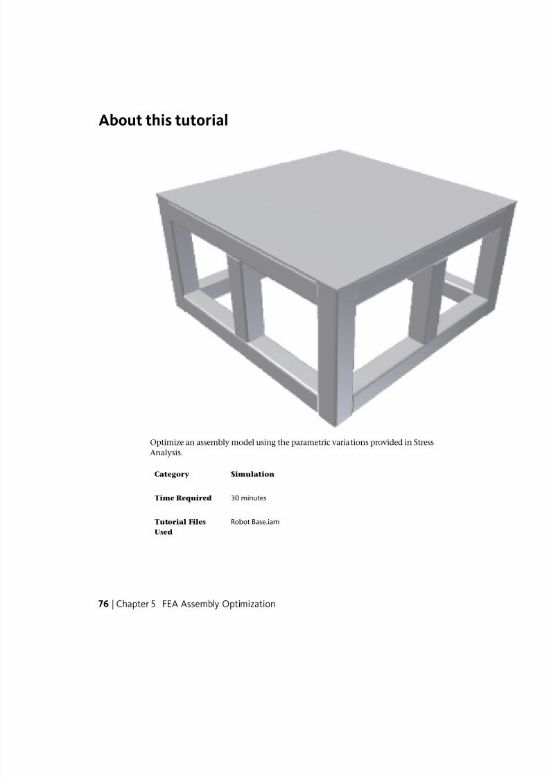
8/20/2019 Stress Analysis INVENTOR
http://slidepdf.com/reader/full/stress-analysis-inventor 82/266
About this tutorial
Optimize an assembly model using the parametric variations provided in Stress
Analysis.
SimulationCategory
30 minutesTime Required
Robot Base.iamTutorial Files
Used
76 | Chapter 5 FEA Assembly Optimization

8/20/2019 Stress Analysis INVENTOR
http://slidepdf.com/reader/full/stress-analysis-inventor 83/266
NOTE Click and read the required Tutorial Files Installation Instructions atht-
tp://www.autodesk.com/inventor-tutorial-data-sets . Then download the tutorial
data sets and the required Tutorial Files Installation Instructions, and install the
datasets as instructed.
Objectives
Minimize the mass of the structure while keeping displacement and stress
within allowable values. Consider safety criteria and profile size changes.
Prerequisites
■ Complete the Part Modal and Stress Analysis tutorial.
■ Familiarize yourself with the ribbon user interface.
Navigation Tips
■
Use Next or Previous at the bottom-left to advance to the next page orreturn to the previous one.
Next (page 77)
Open the Assembly
1 Click ➤
Open.
2 Set the Project File to Tutorial_Files.ipj.
3 Open Assembly Optimization using FEA
➤
Robot Base.iam.
4 On the ribbon, click Environments tab
➤
Begin panel ➤
Stress
Analysis .
Previous (page 76) | Next (page 77)
Define the Simulation
1 On the ribbon, Manage panel, click Create Simulation .
Open the Assembly | 77

8/20/2019 Stress Analysis INVENTOR
http://slidepdf.com/reader/full/stress-analysis-inventor 84/266
2 In the Create New Simulation dialog box, enter the following:
■ Name: Optimization
■ Design Objective: Parametric Dimension
■ Simulation Type: Static Analysis
3 Click OK. A new simulation is created and the browser is populated with
folders.
Previous (page 77) | Next (page 78)
Assign Materials
1 On the ribbon bar, Material panel, click Assign Materials .
2 For the base_plate:1 component, click the Override Material drop-down
list and select Steel. Notice that the Safety Factor column shows that
Yield Strength is used for safety analysis.
3 Right-click the Override Material cell for base_plate:1 and select Copy.
Multi-select the other Override Material cells, right-click, and select
Paste. Multiple instances of a component change with one paste. Click
OK to close the dialog box.
Previous (page 77) | Next (page 78)
Adding ConstraintsAdd constraints to denote mechanical and environmental conditions.
1 On the ribbon bar, Constraints panel, click Fixed .
2 Rotate the model and select the faces that would contact the floor surface.
78 | Chapter 5 FEA Assembly Optimization

8/20/2019 Stress Analysis INVENTOR
http://slidepdf.com/reader/full/stress-analysis-inventor 85/266
3 Click OK.
Previous (page 78) | Next (page 79)
Adding Loads
Define the load where the robot mounts to the base. The mounting plate on
the robot is round, and the base plate is square. To apply the force in the area
where the robot mounts, we must split the base plate face. (This step has
already been performed for you.)
1 On the ribbon bar, Loads panel, click Force .
2 Move the cursor over the center of the base plate component to highlight
the round face. Click to select the face.
Adding Loads | 79

8/20/2019 Stress Analysis INVENTOR
http://slidepdf.com/reader/full/stress-analysis-inventor 86/266
3 In the Force dialog box, for Magnitude, enter 2000 and click OK. Ayellow (default color) glyph denoting the force direction is positioned
at the center of the face.
Previous (page 78) | Next (page 80)
Modify the Mesh
Review the mesh settings and make a minor adjustment.
1 On the ribbon bar, Prepare panel, click Mesh Settings .2 In the Mesh Settings dialog box, click Create Curved Mesh Elements.
This option creates elements that follow geometry curvature.
3 The Use part based measure for Assembly mesh option is checked by
default, which is correct for this simulation. This option produces a
higher mesh resolution in smaller parts, with a resulting increase in mesh
elements overall.
4 Click OK to apply the change and close the dialog box.
Previous (page 79) | Next (page 81)
80 | Chapter 5 FEA Assembly Optimization

8/20/2019 Stress Analysis INVENTOR
http://slidepdf.com/reader/full/stress-analysis-inventor 87/266
Preview the Mesh
Previewing the mesh is an optional step. Perform the mesh preview to examine
the mesh in areas where features are smaller, or where transitions occur, to
ensure an adequate mesh results.
On the ribbon bar, Prepare panel, click Mesh View .
Previous (page 80) | Next (page 82)
Preview the Mesh | 81

8/20/2019 Stress Analysis INVENTOR
http://slidepdf.com/reader/full/stress-analysis-inventor 88/266
Create Parametric Geometry
Produce a range of geometric configurations, involving the width of the model
components, to facilitate weight optimization. First, expose model parameters
for use as simulation parameters.
1 In the Simulation browser, expand the Robot Base.iam node to expose
the components in the assembly. Right-click base_plate:1 and click Show
Parameters.
2 In the Select Parameters dialog box, select the check box next to the
MemberWidth parameter to include the parameter in the parametric
table.
3 Click OK.
Define the parameter range.
1 On the ribbon bar, Manage panel, click Parametric Table .
2 In the Parameters section, base_plate.ipt row, for the MemberWidth
parameter, enter 1-2 in the Values cell. Press Enter to update the row
contents.
82 | Chapter 5 FEA Assembly Optimization

8/20/2019 Stress Analysis INVENTOR
http://slidepdf.com/reader/full/stress-analysis-inventor 89/266
Once the parameter is defined, generate the parametric configurations.
1 In the Parameters section, right-click the MemberWidth row and selectGenerate All Configurations.
2 After the configurations are generated, you can view them using the
Current Value slider.
Create Parametric Geometry | 83

8/20/2019 Stress Analysis INVENTOR
http://slidepdf.com/reader/full/stress-analysis-inventor 90/266
Previous (page 81) | Next (page 84)
Optimization Criteria
As mentioned at the outset, the goal is to minimize the mass using the range
of geometric configurations and safety factor criteria. The Design Constraints
section of the Parametric Table enables access to the results criteria. To add
the first design constraint:
1 If the Parametric Table is not displayed, in the Manage panel, click
Parametric Table.
2 In the Design Constraints section, right-click the row and select Add
Design Constraint.
3 In the Results Component section of the Select Design Constraint dialogbox, select Von Mises Stress. Geometry Selections is set to All Geometry.
Click OK. The result component is listed as a design constraint.
4 In the Max Von Mises Stress row, click the Constraint Type cell to access
the drop-down list. In the drop-down list select Upper limit.
5 In the Limit cell, enter 4.5e+004.
6 In the Safety Factor cell, enter 1.5.
Add Displacement as a design constraint.
1 Right-click a row and click Add Design Constraint.
2 In the Select Design Constraint dialog box, select Displacement. All
Geometry is the default. Click OK.3 In the Constraint Type cell, select Upper limit.
4 In the Limit cell, enter 0.01.
Add Mass as a design constraint.
1 Right-click a row and click Add Design Constraint.
2 In the Select Design Constraint dialog box, select Mass and click OK.
For the Mass design constraint, leave the constraint type as View the
value. The Design Constraints section of the Parametric Table should
look like the following image:
84 | Chapter 5 FEA Assembly Optimization

8/20/2019 Stress Analysis INVENTOR
http://slidepdf.com/reader/full/stress-analysis-inventor 91/266
Close the table.
Previous (page 82) | Next (page 85)
Run the Simulation
1 On the ribbon bar, Solve panel, click Simulate .
2 In the Simulate dialog box, ensure that the simulation will run using
the Smart set of configurations.
3 Click Run.
Previous (page 84) | Next (page 85)
View and Interpret the Results
The Simulation browser Results node is populated with the simulation results.
However, we use the Parametric Table and the visualization capabilities to
assess the design and optimize for mass.
1 On the ribbon bar, Manage panel, click Parametric Table.
2 In the Parametric Table, note the presence of a green circle in two Result
Value cells. A green circle indicates that the Result Value is within the
associated safety factors.
Run the Simulation | 85

8/20/2019 Stress Analysis INVENTOR
http://slidepdf.com/reader/full/stress-analysis-inventor 92/266
3 Change the Mass Constraint Type to Minimize.
The parametric values change to show the configuration with the least
mass that meets the given constraints. In this case, the original profile
width value was 2 inches. The optimized configuration is 1.5 inches,
which reduces the mass.
NOTE If you move the slider to show a current value of 1.0, the table updates
and you see that maximum displacement exceeds the safety factor criteria.
A red square, next to the Result Value, denotes the condition.
Previous (page 85) | Next (page 87)
86 | Chapter 5 FEA Assembly Optimization

8/20/2019 Stress Analysis INVENTOR
http://slidepdf.com/reader/full/stress-analysis-inventor 93/266
View and animate 3D plots
View 3D and XY plots to understand the behavior of the model under the
defined boundary conditions.
After running a simulation, you can perform post-processing tasks using the
assorted commands in the Display panel. You can choose shading options,
display minimum and maximum labels, insert probes, and so on.
The Results node, in the Simulation browser, is populated with the simulation
results based on the criteria you specified. The Von Mises Stress result (default)
is displayed as a 3D color plot.
In this example, because of the connections between profile geometry, stress
concentrations are expected at the joints. To see the stress distribution farther
away from the concentrations, change the Color Bar settings.
1 On the ribbon bar, Display panel, click Color Bar.
2 In the dialog box, uncheck Maximum.
3 Enter 5 in the edit field above the check box. Click Apply.
4 Use the view commands to rotate the model so you can see the underside
of the assembly. Note how the stress is distributed in the members.
View and animate 3D plots | 87

8/20/2019 Stress Analysis INVENTOR
http://slidepdf.com/reader/full/stress-analysis-inventor 94/266
To view other results such as Displacement, double-click the appropriate
browser node to update the display.
For simulations involving parametric dimensions, move the slider to various
parameter values to display the associated results.
Previous (page 85) | Next (page 88)
View XY Plots
XY plots show a result component over the range of a parameter. To view an
XY plot, right-click the parameter row and select XY Plot.
88 | Chapter 5 FEA Assembly Optimization
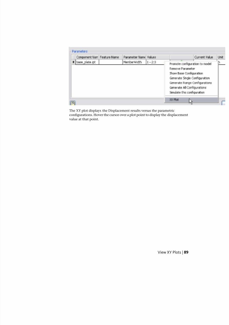
8/20/2019 Stress Analysis INVENTOR
http://slidepdf.com/reader/full/stress-analysis-inventor 95/266
The XY plot displays the Displacement results versus the parametric
configurations. Hover the cursor over a plot point to display the displacementvalue at that point.
View XY Plots | 89

8/20/2019 Stress Analysis INVENTOR
http://slidepdf.com/reader/full/stress-analysis-inventor 96/266
Previous (page 87) | Next (page 90)
Summary
In this tutorial, you learned to:
■ Create a simulation.
■ Specify materials, constraints, and forces.
■ Specify parametric dimensions and generate configurations.
■ View different configurations as 3D color plots and XY plots.
What Next?
90 | Chapter 5 FEA Assembly Optimization

8/20/2019 Stress Analysis INVENTOR
http://slidepdf.com/reader/full/stress-analysis-inventor 97/266
If you have not completed the other FEA tutorials, why not do so now? Or,
if you have not used Dynamic Simulation, work through those tutorials and
learn how to use that simulation output in the Stress Analysis environment.
Consider how this process applies to the products you design and manufacture.
Previous (page 88)
Summary | 91

8/20/2019 Stress Analysis INVENTOR
http://slidepdf.com/reader/full/stress-analysis-inventor 98/266
92

8/20/2019 Stress Analysis INVENTOR
http://slidepdf.com/reader/full/stress-analysis-inventor 99/266
Stress Analysis Contacts
About this tutorial
Use contacts to simulate interactions between assembly components in Inventor
Stress Analysis.
SimulationCategory
45 minutesTime Required
Caulk Gun.iamTutorial Files Used
NOTE Click and read the required Tutorial Files Installation Instructions atht-
tp://www.autodesk.com/inventor-tutorial-data-sets . Then download the tutorial data
sets and the required Tutorial Files Installation Instructions, and install the datasets
as instructed.
Prerequisites
Perform some of the other Stress Analysis tutorials to become familiar with the
Stress Analysis environment..
Navigation Tips
■ Use Next or Previous at the bottom-left to advance to the next page or return
to the previous one.
Next (page 94)
6
93

8/20/2019 Stress Analysis INVENTOR
http://slidepdf.com/reader/full/stress-analysis-inventor 100/266
Overview
In the structural analysis of an assembly involving multiple parts, you create
contacts to define the relationship between the parts. Contacts transfer load
between parts while preventing parts from penetrating each other. Contacts
can simulate interaction between bodies that separate or come into contact
during loading. Without contacts, parts do not interact with each other in
the simulation.
There are several different contact types you can use to simulate the physical
behavior of an assembly. This tutorial presents an assembly modeled with
many of the types of contact available in Inventor Stress Analysis. The contacts
have already been created, either automatically or manually, in the model.
Previous (page 93) | Next (page 94)
Open the Assembly
A model of a caulk gun illustrates different contact types and how to use them
in a static, structural analysis.
1 Click ➤
Open.
2 Set the Project File to Tutorial_Files.ipj.
3 Open Stress Analysis Contacts
➤
Caulk Gun.iam.
94 | Chapter 6 Stress Analysis Contacts

8/20/2019 Stress Analysis INVENTOR
http://slidepdf.com/reader/full/stress-analysis-inventor 101/266
Open the Assembly | 95

8/20/2019 Stress Analysis INVENTOR
http://slidepdf.com/reader/full/stress-analysis-inventor 102/266
Previous (page 94) | Next (page 96)
How a Caulk Gun Works
We considered the following mechanics of the caulk gun when creating the
simulation.
96 | Chapter 6 Stress Analysis Contacts

8/20/2019 Stress Analysis INVENTOR
http://slidepdf.com/reader/full/stress-analysis-inventor 103/266
How a Caulk Gun Works | 97

8/20/2019 Stress Analysis INVENTOR
http://slidepdf.com/reader/full/stress-analysis-inventor 104/266
1 User holds the handle [1] and pulls back on the trigger [2].
2 The pin end of the trigger [3] pushes the actuator [4] forward.
3 The actuator tightly engages the plunger [5] and pushes it forward.
4 The plunger head [6] pushes the caulk tube bottom.
5 The tube is held in place by a ring [7] at the end of the caulk gun.
Previous (page 94) | Next (page 99)
98 | Chapter 6 Stress Analysis Contacts

8/20/2019 Stress Analysis INVENTOR
http://slidepdf.com/reader/full/stress-analysis-inventor 105/266
Assembly Simulation
The caulk gun is an assembly which consists of several parts, some of which
can move. Several operational scenarios can exist for the caulk gun, but we
chose to simulate the assembly in a static equilibrium state.
This simulation investigates when the trigger is pulled and the pushing force
on the bottom of the caulk tube is about to overcome the internal tube
resistance. At this instant, just before caulk exits the tube, the assembly is in
static equilibrium.
On the ribbon, click Environments tab
➤
Begin panel ➤
Stress
Analysis to enter the Stress Analysis environment.
Expand Caulk Gun.iam in the Stress Analysis browser. We exclude the
following components from the simulation:
■ Caulk Tube [8]
■ Actuator Spring [9] (not modeled, but simulated with Spring contact)
■ Lock Spring [10]
■ Lock [11]
Assembly Simulation | 99

8/20/2019 Stress Analysis INVENTOR
http://slidepdf.com/reader/full/stress-analysis-inventor 106/266
Previous (page 96) | Next (page 100)
Contact Types
Inventor Stress Analysis provides the following Contact types:
■ Bonded
■ Separation
■ Sliding / No Separation
■ Separation / No Sliding
■ Shrink Fit / Sliding
■ Shrink Fit / No Sliding
100 | Chapter 6 Stress Analysis Contacts

8/20/2019 Stress Analysis INVENTOR
http://slidepdf.com/reader/full/stress-analysis-inventor 107/266
■ Spring
In the Stress Analysis browser, expand the Contacts node to view the contacttypes currently in use for the caulk gun simulation. As you create or edit
contacts, they are added under existing contact type nodes or to newly created
nodes.
Contact Types | 101

8/20/2019 Stress Analysis INVENTOR
http://slidepdf.com/reader/full/stress-analysis-inventor 108/266
In the browser, right-click a contact and select Edit Contact. The Edit
Automatic Contact or Edit Manual Contact dialog box displays and shows the
available contact types:
Previous (page 99) | Next (page 102)
Bonded Contact
The Bonded contact simulates rigid bonding of faces to each other. Typical
Bonded contacts include weld or glue joints between two parts.
In the model, the Front Frame-Main Frame and the Front Frame-Handle
interfaces are weld joints, as shown in the following image. You use Bonded
contacts to simulate these joints in the simulation.
102 | Chapter 6 Stress Analysis Contacts

8/20/2019 Stress Analysis INVENTOR
http://slidepdf.com/reader/full/stress-analysis-inventor 109/266
Previous (page 100) | Next (page 103)
Separation Contact
The Separation contact allows separation between parts but prohibits part
penetration.
In the model, the pin end of the trigger contacts the actuator. When you pull
the trigger, the pin end of the trigger pushes the actuator forward. When the
trigger is released, the pin end and the actuator can separate. Since the pin
end cannot penetrate the actuator and separation can occur between the parts,
the contact relationship is simulated with the Separation contact.
Separation Contact | 103

8/20/2019 Stress Analysis INVENTOR
http://slidepdf.com/reader/full/stress-analysis-inventor 110/266
Previous (page 102) | Next (page 104)
Sliding and No Separation Contact
The Sliding/No Separation contact allows relative sliding between contact
faces, but prohibits separation.
104 | Chapter 6 Stress Analysis Contacts

8/20/2019 Stress Analysis INVENTOR
http://slidepdf.com/reader/full/stress-analysis-inventor 111/266
Sliding/No Separation can occur between planar faces like the Trigger-Handle
interface.
Sliding and No Separation Contact | 105

8/20/2019 Stress Analysis INVENTOR
http://slidepdf.com/reader/full/stress-analysis-inventor 112/266
It can also occur between circular faces such as the Pin-Handle and Pin-Trigger
interfaces.
106 | Chapter 6 Stress Analysis Contacts

8/20/2019 Stress Analysis INVENTOR
http://slidepdf.com/reader/full/stress-analysis-inventor 113/266
Previous (page 103) | Next (page 107)
Separation and No Sliding Contact
The Separation/No Sliding contact allows contact faces to separate, but
prohibits relative sliding when they touch.
For the Actuator-Plunger interface, the Separation/No Sliding contact is
appropriate. When the trigger is pulled, the actuator is pushed forward. This
results in separation between the top surface of the plunger and the actuator.
At the same time, engagement occurs between the bottom surface of the
plunger and the actuator. It is reasonable to assume that the
engagement/separation occurs without slippage between the actuator and
plunger.
In the following image, note that the surfaces of the plunger and actuator are
split into multiple faces. In this manner, the contact surfaces are more explicitly
defined.
Separation and No Sliding Contact | 107

8/20/2019 Stress Analysis INVENTOR
http://slidepdf.com/reader/full/stress-analysis-inventor 114/266
Previous (page 104) | Next (page 108)
Shrink Fit and No Sliding Contact
The Shrink Fit/No Sliding contact simulates conditions like Separation/No
Sliding with the parts in an initial state of interference.
108 | Chapter 6 Stress Analysis Contacts

8/20/2019 Stress Analysis INVENTOR
http://slidepdf.com/reader/full/stress-analysis-inventor 115/266
The model has a ring that tightly fits the front frame and prevents the caulk
tube from exiting the caulk gun when the plunger moves forward. The front
face of the ring registers against the front frame without penetration. Therefore,this interface is simulated with the Separation contact.
The outer diameter of the ring has an interference fit with the front frame.
The ring is press fit into the frame so that it remains in position without a
caulk gun in place. This press fit allows the operator to push the ring out easily
and replace it with a different size, as appropriate. The outer diameter of the
ring and the front frame can separate without sliding. Since they are initially
in a state of interference, the Shrink Fit/No Sliding contact is appropriate.
Shrink Fit and No Sliding Contact | 109

8/20/2019 Stress Analysis INVENTOR
http://slidepdf.com/reader/full/stress-analysis-inventor 116/266
Previous (page 107) | Next (page 110)
Spring Contact
The Spring contact simulates conditions of a spring between two faces.
In the model, the actuator spring is simulated using a Spring contact. The use
of the Spring contact eliminates complexities associated with modeling the
physical spring part.
110 | Chapter 6 Stress Analysis Contacts

8/20/2019 Stress Analysis INVENTOR
http://slidepdf.com/reader/full/stress-analysis-inventor 117/266
Previous (page 108) | Next (page 111)
Loads and Constraints
With the contacts defined, proceed further with the model analysis.
To use the caulk gun, you hold the handle and pull the trigger. From the static
analysis point of view, the components are under force and deform before
the plunger head moves the bottom of the tube. We can reasonably assume
that the components deform relative to the main frame. As such, we can apply
a:
■ Fixed constraint on the main frame edge [12]
■ Force on the handle [13]
■Force on the trigger [14]
■ Force on the plunger head [15]
■ Force on the ring [16]
Loads and Constraints | 111

8/20/2019 Stress Analysis INVENTOR
http://slidepdf.com/reader/full/stress-analysis-inventor 118/266
The tube is held in place by the front frame, ring, and plunger head. When
the force from plunger head is large enough, the bottom of the tube moves
further into the tube and pushes caulk out of the nozzle. For the static analysis,
we simulate the instant at which the force on the tube bottom is in equilibrium
with the tube resistance. Before the tube bottom moving, we examine thestress and deformation of the whole structure and components.
Previous (page 110) | Next (page 112)
Simulation Results
1 On the Stress Analysis tab, Solve panel, click Simulate .
2 On the Simulate dialog box, click Run to begin the simulation.
The Simulate dialog box remains open, displaying the progress bar, until thecomputation is complete.
112 | Chapter 6 Stress Analysis Contacts
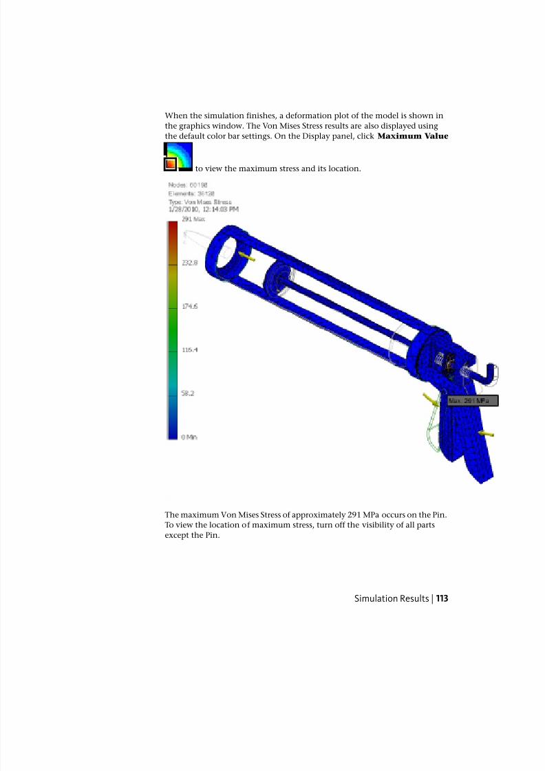
8/20/2019 Stress Analysis INVENTOR
http://slidepdf.com/reader/full/stress-analysis-inventor 119/266
When the simulation finishes, a deformation plot of the model is shown in
the graphics window. The Von Mises Stress results are also displayed using
the default color bar settings. On the Display panel, click Maximum Value
to view the maximum stress and its location.
The maximum Von Mises Stress of approximately 291 MPa occurs on the Pin.
To view the location of maximum stress, turn off the visibility of all parts
except the Pin.
Simulation Results | 113

8/20/2019 Stress Analysis INVENTOR
http://slidepdf.com/reader/full/stress-analysis-inventor 120/266
As this stress is greater than the Pin material (steel) yield strength of 207 MPa,
the analysis indicates the Pin will yield. To meet strength criteria, you modify
the design or change the Pin material.
NOTE In this tutorial, the model is intended to illustrate the contact types and
their application. Some contact areas such as the Plunger-Actuator interface are
small. Take care when providing spring stiffness and force values as the
displacement and stress results are sensitive to parameter values. Also note that
some parts may have areas of large deformation, which are better suited to anonlinear analysis.
Previous (page 111) | Next (page 114)
Summary
In this tutorial, you learned about Inventor Stress Analysis contacts and how
they simulate interactions between assembly components.
What Next?
To investigate design workflows further using Inventor Stress Analysis, refer
to other Help documents and tutorials included with Inventor.
114 | Chapter 6 Stress Analysis Contacts

8/20/2019 Stress Analysis INVENTOR
http://slidepdf.com/reader/full/stress-analysis-inventor 121/266
Previous (page 112)
Summary | 115

8/20/2019 Stress Analysis INVENTOR
http://slidepdf.com/reader/full/stress-analysis-inventor 122/266
116

8/20/2019 Stress Analysis INVENTOR
http://slidepdf.com/reader/full/stress-analysis-inventor 123/266
Frame Analysis
About this tutorial
Perform basic structural analysis of your frame structures with respect to
deformations and stresses.
SimulationCategory
30 minutesTime Required
7
117

8/20/2019 Stress Analysis INVENTOR
http://slidepdf.com/reader/full/stress-analysis-inventor 124/266
analyze_frame.iamTutorial File Used
NOTE Click and read the required Tutorial Files Installation Instructions atht-
tp://www.autodesk.com/inventor-tutorial-data-sets . Then download the tutorial
data sets and the required Tutorial Files Installation Instructions, and install the
datasets as instructed.
The Frame Analysis environment is a special environment within assembly
and weldment files. The environment has commands unique to its purpose.
You can access the tools from the Design or Environments tabs.
When you open a Frame Analysis and set up your simulation, the assembly
frame model is automatically converted to a simplified model of nodes and
beams. The graphics window displays beams, nodes, and the gravity glyph.
Then, you define the boundary conditions (consisting of loads and constraints).You can also change beam materials, and specify connections (releases and
rigid links). Once these inputs are entered, you can run the simulation and
view the behavior relative to the conditions you defined.
Objectives
■ Create a simulation.
■ Evaluate and assign materials.
■ Evaluate and assign beam properties.
■ Add loads.
■ Add constraints.
■ Run a simulation.
■ View the results.
Prerequisites
■ Know how to use the Quick Access toolbar, tabs, and panels on the ribbon,
model browser, and context menus.
■ Know how to navigate the model space with the various view tools.
■ Know how to specify and edit project files.
■ Complete the Frame Generator tutorial.
■ See the Help topics for further information.
118 | Chapter 7 Frame Analysis

8/20/2019 Stress Analysis INVENTOR
http://slidepdf.com/reader/full/stress-analysis-inventor 125/266
Navigation Tips
■ Use Next or Previous at the bottom-left to advance to the next page or
return to the previous one.
Next (page 119)
Open the Assembly
To begin, open the assembly to analyze.
1 Click the Open command on the Quick Access toolbar.
2 Set the Project File to tutorial_files.ipj
3 Select Frame Analysis 1
➤
analyze_frame.iam.4 Click Open.
5 Click Save as to save the file with a different name, such as:
analyze_frame_tutorial.iam.
Previous (page 117) | Next (page 119)
Frame Analysis Environment
We are ready to enter the Frame Analysis environment.
1 On the ribbon, click Environments tab ➤
Begin panel ➤
Frame
Analysis .
Initially, there are only three commands enabled: Create Simulation,
Frame Analysis Settings, and Finish Frame Analysis. For now,
create a simulation and review the settings in the next step.
2 On the Manage panel, click the Create Simulation command.
The Create New Simulation dialog box opens.
You can use the dialog box settings to specify a unique name, simulation
type, and other simulation parameters.
Open the Assembly | 119

8/20/2019 Stress Analysis INVENTOR
http://slidepdf.com/reader/full/stress-analysis-inventor 126/266
There are two types of Frame Analysis.
■ Static Analysis evaluates structural loading conditions.
■ Modal Analysis evaluates natural frequency modes.
NOTE On the Model State tab, you specify the Design View,
Positional, and Level of Detail to use for the simulation. Also, you can
specify the iAssembly member to be associated with the simulation. The
settings can be different for each simulation.
3 Click OK to accept the default settings for this simulation.
The Inventor model is automatically converted into idealized nodes and
beams, and a simulation is created. A gravity symbol also displays.
120 | Chapter 7 Frame Analysis
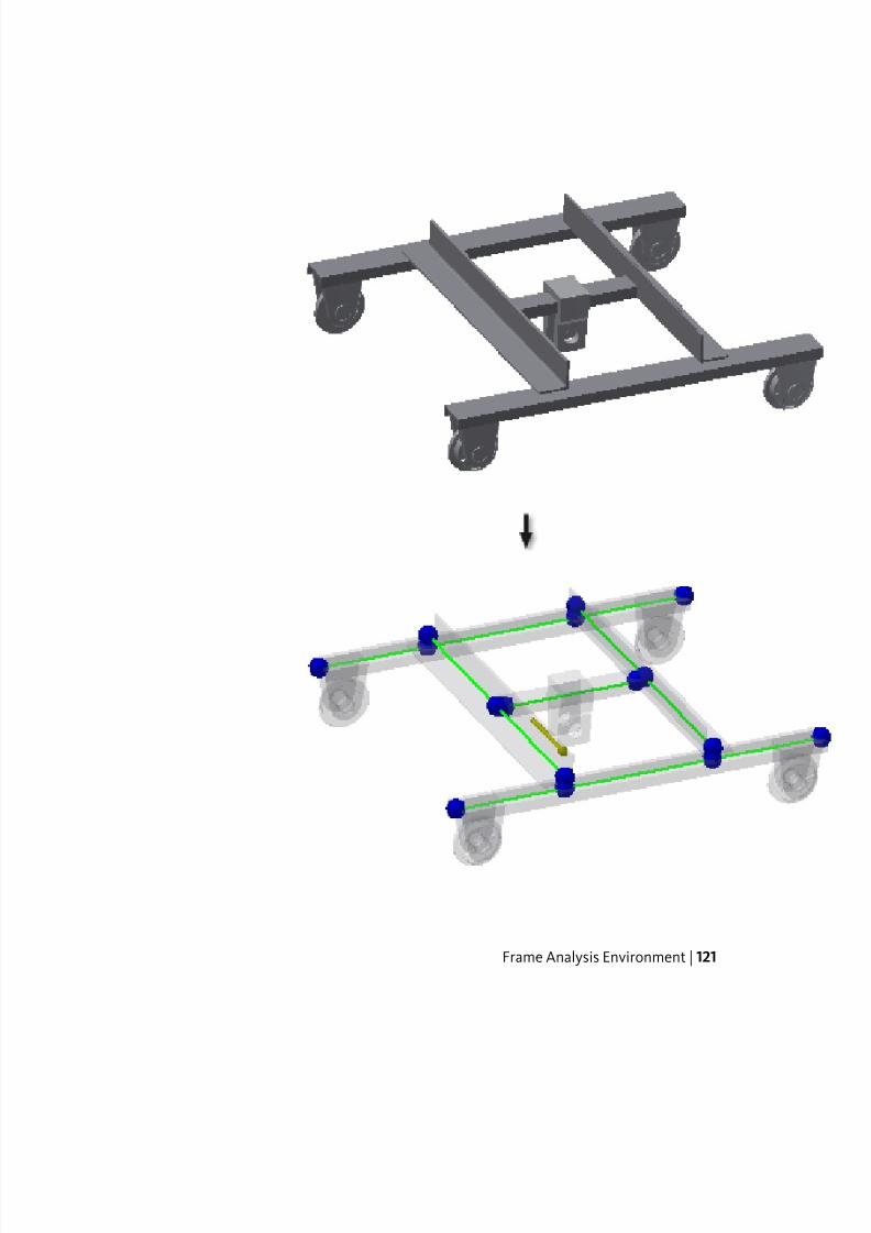
8/20/2019 Stress Analysis INVENTOR
http://slidepdf.com/reader/full/stress-analysis-inventor 127/266
Frame Analysis Environment | 121

8/20/2019 Stress Analysis INVENTOR
http://slidepdf.com/reader/full/stress-analysis-inventor 128/266
The browser populates with a hierarchical structure of the assembly and
analysis-related folders.
Most of the commands in the ribbon panels are now enabled for use. Disabled
commands enable after you run the simulation.
Previous (page 119) | Next (page 122)
Frame Analysis Settings
Frame Analysis settings apply to all new simulations. Whenever a new frame
simulation is started, these preferences are used.
In the Frame Analysis Settings dialog box, you can specify:
■ If Heads up Display is the preferred method used during input and edit.
■ Colors for displayed boundary conditions, nodes, rigid links, gravity.
■ Scale for displayed nodes, loads, and constraints.
■ Default visibility settings for all components (beams and other parts) after
the conversion.
■ Solver method used for beam releases.
■ Display of diagrams.
In this tutorial, we use the dialog boxes for input of boundary conditions
values.
On the ribbon, click Frame Analysis Settings in the Settings panel.
In the General tab, clear the Use HUD in Application check box. Click
OK.
Previous (page 119) | Next (page 122)
Assign Materials
The next step is to look at the model materials and adjust the material.
For this simulation, we only make a minor material change using materials
that are fully defined.
122 | Chapter 7 Frame Analysis

8/20/2019 Stress Analysis INVENTOR
http://slidepdf.com/reader/full/stress-analysis-inventor 129/266
Before you perform simulations, ensure that your material definitions are
complete for those materials being analyzed. When a material is not completely
or inadequately defined, a warning message displays in the Status folder inthe browser. You cannot run a simulation until you change the material.
NOTE You cannot edit a material if the project setting Use Styles Library is
set to Read-Only. To change the setting requires exiting the tutorial. In this
tutorial, we use a material that is already fully defined. You can modify the other
materials at a later time.
1 In the browser, expand the Beams folder, and select Beam:1. Right-click
and select Beam Materials. In the Beam Material dialog box, select
the beam (DIN U 200 00000001.ipt) in the Beams area.
NOTE Beam Material dialog box is also accessible when you click Material
on the Beams panel in the ribbon.
2 Check the Customize box.
NOTE The Customize check box is only available when the parent beam is
selected.
3 In the drop-down menu in the Material area, select Stainless Steel,
Austenitic.
4 Click OK to exit the Beam Material dialog box.
The browser Materials folder receives a Stainless Steel, Austenitic - DIN
U 200 00000001.ipt folder added with all the components referencing thatmaterial listed within that folder. If you delete individual components from
the folder, their material reverts to the assembly assigned material.
Previous (page 122) | Next (page 124)
Assign Materials | 123
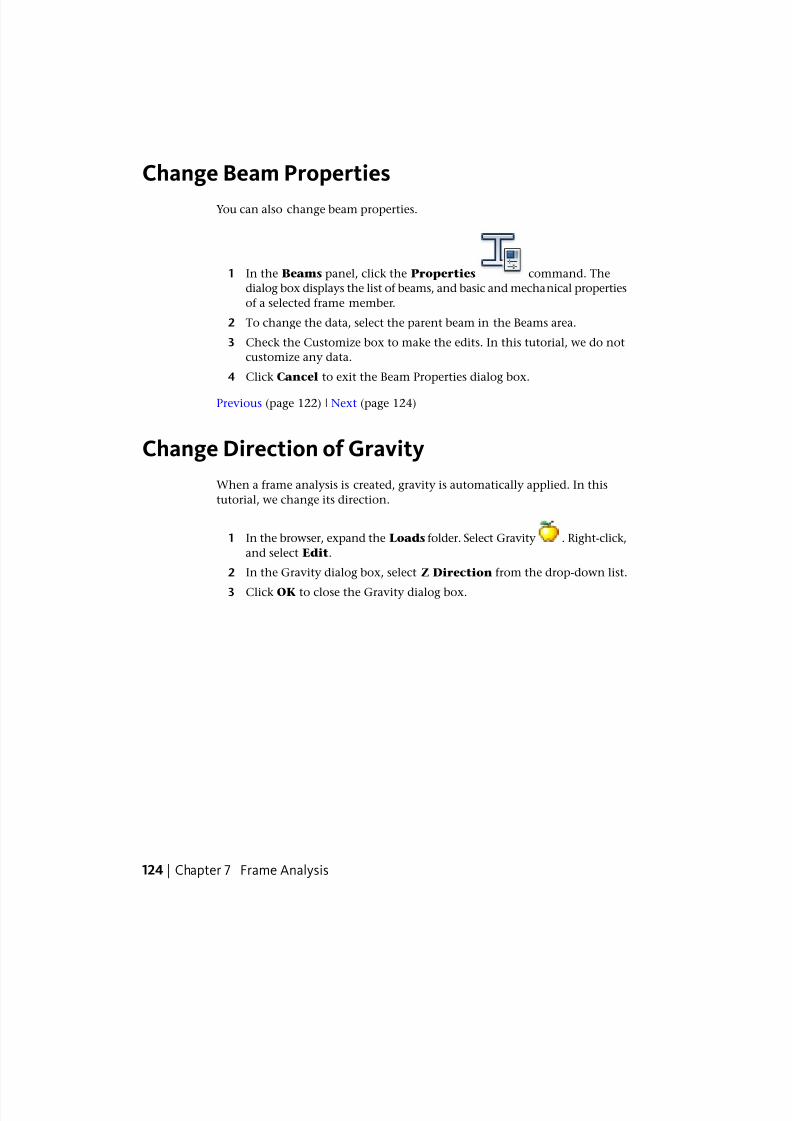
8/20/2019 Stress Analysis INVENTOR
http://slidepdf.com/reader/full/stress-analysis-inventor 130/266
Change Beam Properties
You can also change beam properties.
1 In the Beams panel, click the Properties command. The
dialog box displays the list of beams, and basic and mechanical properties
of a selected frame member.
2 To change the data, select the parent beam in the Beams area.
3 Check the Customize box to make the edits. In this tutorial, we do not
customize any data.
4 Click Cancel to exit the Beam Properties dialog box.
Previous (page 122) | Next (page 124)
Change Direction of Gravity
When a frame analysis is created, gravity is automatically applied. In this
tutorial, we change its direction.
1 In the browser, expand the Loads folder. Select Gravity . Right-click,
and select Edit.
2 In the Gravity dialog box, select Z Direction from the drop-down list.
3 Click OK to close the Gravity dialog box.
124 | Chapter 7 Frame Analysis

8/20/2019 Stress Analysis INVENTOR
http://slidepdf.com/reader/full/stress-analysis-inventor 131/266
Previous (page 124) | Next (page 125)
Add Constraints
Next, we define the boundary conditions by adding structural constraints and
loads. We start with constraints first.
NOTE Constraints are required for frame simulations. If you start a simulation
without constraints, a dialog box displays the error message: No constraints
defined.
1 In the Constraints panel, click Pinned . The dialog box
displays with the Origin selector active.
2 Select the beam as shown in the image. The preview of the pinned
constraint displays.
Add Constraints | 125
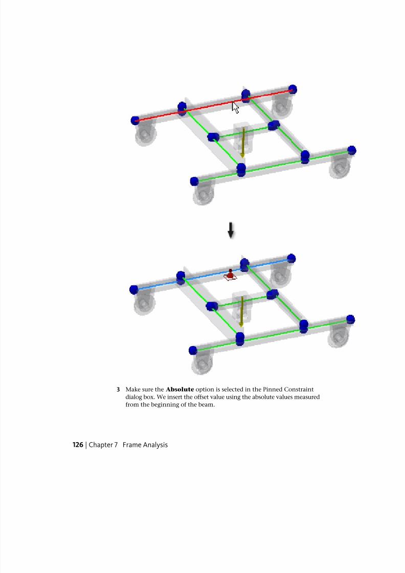
8/20/2019 Stress Analysis INVENTOR
http://slidepdf.com/reader/full/stress-analysis-inventor 132/266
3 Make sure the Absolute option is selected in the Pinned Constraint
dialog box. We insert the offset value using the absolute values measured
from the beginning of the beam.
126 | Chapter 7 Frame Analysis

8/20/2019 Stress Analysis INVENTOR
http://slidepdf.com/reader/full/stress-analysis-inventor 133/266
NOTE You can use the Local Systems command in the Display
panel to show the beam coordinate systems to define the beginning of the
beams.
4 In the Pinned Constraint dialog box, set Offset to 170 mm, and click
OK. The Pinned constraint is applied.
5 Insert the second pinned constraint to the same beam. Again, click
Pinned in the Constraints panel.
6 Select the same beam, and set Offset to 2330 mm. Click OK.
Previous (page 124) | Next (page 128)
Add Constraints | 127

8/20/2019 Stress Analysis INVENTOR
http://slidepdf.com/reader/full/stress-analysis-inventor 134/266
Add Constraints to the Next Beam
We must insert pinned constraints to the opposite side of the cart.
1 In the browser, select Constraints folder. Right-click and select Pinned
Constraint .
2 Select the beam as shown in the following image. The preview of the
pinned constraint displays.
128 | Chapter 7 Frame Analysis

8/20/2019 Stress Analysis INVENTOR
http://slidepdf.com/reader/full/stress-analysis-inventor 135/266
3 In the Pinned Constraint dialog box, set Offset to 170 mm, and click
OK. Pinned constraint is applied.
4 Insert the second pinned constraint to the same beam. In the browser,
select Constraints folder. Right-click and select Pinned Constraint
.
5 Select the same beam, and set Offset to 2330 mm. Click OK.
We applied all necessary constraints so we can add loads now.
Previous (page 125) | Next (page 129)
Add Loads
Now assign loads on the components.
1 In the Loads panel, click Force . The dialog box displays with
the Origin selector active.
Add Loads | 129

8/20/2019 Stress Analysis INVENTOR
http://slidepdf.com/reader/full/stress-analysis-inventor 136/266
2 Select the middle beam where the force is acting.
3 In the dialog box, enter 500 N for the Magnitude value, and 0 degrees
for Angle of Plane.
NOTE The Angle of plane specifies the rotation of the XY plane where the
force is acting. Angle in plane defines the angle of the applied force from
the Z-axis.
4 Click the More button to expand the dialog box to display additional
controls for specifying the force vector. In the Offset area, check the
Relative box. You can now position the force to the middle of theselected beam. Enter 0.5 in the Offset edit field in the upper part of the
130 | Chapter 7 Frame Analysis

8/20/2019 Stress Analysis INVENTOR
http://slidepdf.com/reader/full/stress-analysis-inventor 137/266
dialog box. Click OK to exit the Force dialog box.
Previous (page 128) | Next (page 131)
Run the Simulation
We are now ready to run the simulation.
In the Solve panel, click Simulate . The progress bar displays
showing the status of the simulation.
Previous (page 129) | Next (page 132)
Run the Simulation | 131
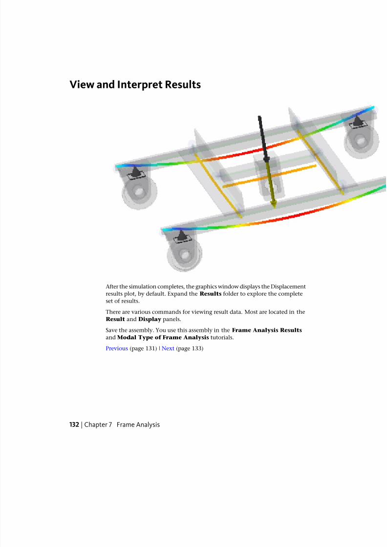
8/20/2019 Stress Analysis INVENTOR
http://slidepdf.com/reader/full/stress-analysis-inventor 138/266
View and Interpret Results
After the simulation completes, the graphics window displays the Displacementresults plot, by default. Expand the Results folder to explore the complete
set of results.
There are various commands for viewing result data. Most are located in the
Result and Display panels.
Save the assembly. You use this assembly in the Frame Analysis Results
and Modal Type of Frame Analysis tutorials.
Previous (page 131) | Next (page 133)
132 | Chapter 7 Frame Analysis

8/20/2019 Stress Analysis INVENTOR
http://slidepdf.com/reader/full/stress-analysis-inventor 139/266
Summary
The previous image is what you see if you look at the Fx Forces results for this
simulation.
Now you have a basic understanding of the typical workflow in the frame
analysis environment. This workflow includes:
■ Creating a simulation.
■ Assigning materials as overrides of the existing material.
■ Adding constraints and loads, sometimes called boundary conditions.
■ Running a simulation.
■ Viewing the results.
What Next? As a next step, explore the tools available for viewing and
interpreting results. The Frame Analysis Results tutorial takes you through
these topics.
Summary | 133

8/20/2019 Stress Analysis INVENTOR
http://slidepdf.com/reader/full/stress-analysis-inventor 140/266
Previous (page 132)
134 | Chapter 7 Frame Analysis

8/20/2019 Stress Analysis INVENTOR
http://slidepdf.com/reader/full/stress-analysis-inventor 141/266
Frame Analysis Results
About this tutorial
SimulationCategory
15 minutesTime Required
analyze_frame_tutorial.iamTutorial File Used
8
135

8/20/2019 Stress Analysis INVENTOR
http://slidepdf.com/reader/full/stress-analysis-inventor 142/266
NOTE Click and read the required Tutorial Files Installation Instructions atht-
tp://www.autodesk.com/inventor-tutorial-data-sets . Then download the tutorial
data sets and the required Tutorial Files Installation Instructions, and install the
datasets as instructed.
Objectives
■ Open a simulation.
■ View and interpret the results.
■ Display and edit diagrams.
■ View beam detail.
■ Adjust displacement display.
■ Display maximal and minimal values in the graphics window.
■ Animate results.
■ Generate report.
Prerequisites
■ Complete the Frame Analysis tutorial.
■ Know how to use the Quick Access toolbar, tabs and panels on the ribbon,
model browser, and context menus.
■ Know how to specify and edit project files.
■ See the Help topics for further information.
Navigation Tips
■ Use Next or Previous at the bottom-left to advance to the next page or
return to the previous one.
Next (page 136)
Get Started
To begin, open the assembly to analyze.
1 Click the Open command on the Quick Access toolbar.
2 Set the Project File to tutorial_files.ipj
3 Select Frame Analysis 1 ➤
analyze_frame_tutorial.iam.
136 | Chapter 8 Frame Analysis Results

8/20/2019 Stress Analysis INVENTOR
http://slidepdf.com/reader/full/stress-analysis-inventor 143/266
NOTE This assembly was created during Frame Analysis tutorial.
4 Click Open.
Previous (page 135) | Next (page 137)
Frame Analysis Environment
We are ready to enter the Frame Analysis environment.
On the ribbon, click Environments tab
➤
Begin panel
➤
Frame Analysis
.
We created a simulation during the Frame Analysis tutorial so the modelwith simulation results displays. The displacement results plot displays in the
graphics window by default.
Frame Analysis Environment | 137

8/20/2019 Stress Analysis INVENTOR
http://slidepdf.com/reader/full/stress-analysis-inventor 144/266
The browser populates with a hierarchical structure of the assembly and
analysis-related folders.
All the commands in the ribbon panels are now enabled for use. We can usethe commands for viewing and interpreting results.
Previous (page 136) | Next (page 139)
138 | Chapter 8 Frame Analysis Results

8/20/2019 Stress Analysis INVENTOR
http://slidepdf.com/reader/full/stress-analysis-inventor 145/266

8/20/2019 Stress Analysis INVENTOR
http://slidepdf.com/reader/full/stress-analysis-inventor 146/266
Display Maximum and Minimum Values
Minimum and maximum values quickly show the locations of load extremes.
In the Display panel, click Max Value . In the graphics window, a
label with a leader points to the location of the maximum value.
In the Display panel, click Min Value . In the graphics window, a
label with a leader points to the location of the minimum value.
NOTE You can drag the labels to different locations.
The following image shows maximum and minimum values for the
Displacement results plot.
140 | Chapter 8 Frame Analysis Results

8/20/2019 Stress Analysis INVENTOR
http://slidepdf.com/reader/full/stress-analysis-inventor 147/266
Cancel the selection of the Max Value and Mix Value options in the Displaypanel to hide the values.
Previous (page 139) | Next (page 141)
View Beam Detail
You can display detailed results for the selected beams. In the Result panel,
click Beam Detail .
First, select a beam whose results you want to display. Select a beam as shown
in the following image.
View Beam Detail | 141

8/20/2019 Stress Analysis INVENTOR
http://slidepdf.com/reader/full/stress-analysis-inventor 148/266
In the Diagram Selection area, select the result data you want to display
as a diagram. Select a particular force, moment, or stress to display its diagram,
Fz for example. The displayed diagram is for viewing only and cannot be
edited.
A complete list of beam results displays on the right side of the dialog box.
Click OK to close the dialog box.
Previous (page 140) | Next (page 142)
Display and Edit Diagrams
To display results for a given beam, you can add user-defined diagrams to the
graphics window. In the Result panel, click Diagram .
142 | Chapter 8 Frame Analysis Results

8/20/2019 Stress Analysis INVENTOR
http://slidepdf.com/reader/full/stress-analysis-inventor 149/266
In the Beams area, select how you want to specify which beams are included
in the diagrams. In this tutorial, check the Selected Beams box, and select
the beam as shown in the following image.
Now, select which results you want to display. Check the Fx and Fy boxes inthe Loads area.
Display and Edit Diagrams | 143

8/20/2019 Stress Analysis INVENTOR
http://slidepdf.com/reader/full/stress-analysis-inventor 150/266
Click OK to close the Diagram dialog box.
You can adjust the display of beam diagrams in the Diagram Scales dialogbox. In the browser, select Diagrams, right-click, and select Diagram Scales
. Use the Expand, Contract, and Normalize buttons to adjust the scale of
diagrams. Click OK to see the change in the scale in displayed diagrams.
Previous (page 141) | Next (page 144)
Adjust Displacement Display
You can scale the model deformation using the options in the Adjust
Displacement Display drop-down list in the Display panel.
Expand the Results folder, and double-click the Displacement browser node.
144 | Chapter 8 Frame Analysis Results

8/20/2019 Stress Analysis INVENTOR
http://slidepdf.com/reader/full/stress-analysis-inventor 151/266
Select a multiple to improve the view of the deformation of the model.
In the following image, the Adjusted x0.5 option is selected.
In the following image, the Adjusted x5 option is selected.
Adjust Displacement Display | 145

8/20/2019 Stress Analysis INVENTOR
http://slidepdf.com/reader/full/stress-analysis-inventor 152/266
Previous (page 142) | Next (page 146)
Animate the Results
Now, create an animation of the results.
1 Click Animate in the Result panel.
2 In the Animate Results dialog box, specify number of steps. Set the Steps
edit field to 8.
3 Specify the playback speed. Select Normal in the Speed drop-down
menu.
4 Click the Play command to see the animation. You can pause
playback.
146 | Chapter 8 Frame Analysis Results

8/20/2019 Stress Analysis INVENTOR
http://slidepdf.com/reader/full/stress-analysis-inventor 153/266
5 When you finish the displacement animation, click OK to exit the
animation playback.
The Animate Results dialog box also has options for displaying the original
wireframe with the plot. You can also record the animation to present or retain
for records.
Previous (page 144) | Next (page 147)
Generate Report
We can generate a report of the simulation results which includes all the
simulation data and outputs.
1 Click Report in the Publish panel.
2 On the General tab, check the Custom box.
3 Switch to the Simulations tab, and make sure the Material and Cross
Section in the tree are selected.
4 Switch to the Format tab and make sure the Web page – multiple
files (.html) option is selected in the Report Format drop-down menu.
5 Click OK to close the dialog box and create the HTML report.
Report contains text and PNG images that represent a static snapshot of the
analysis results.
Previous (page 146) | Next (page 148)
Generate Report | 147

8/20/2019 Stress Analysis INVENTOR
http://slidepdf.com/reader/full/stress-analysis-inventor 154/266
Summary
Now you have an understanding of the tools you can use to view and interpret
results of frame analysis. You know how to:
■ Display and edit diagrams.
■ View beam detail.
■ Adjust displacement display.
■ Display maximal and minimal values in the graphics window.
■ Animate results.
■ Generate report.
What Next? As a next step, look into creating advanced connections (releases
and rigid links), and adding custom nodes to the beam model. The Frame
Analysis Connections tutorial takes you through these topics.
Previous (page 147)
148 | Chapter 8 Frame Analysis Results

8/20/2019 Stress Analysis INVENTOR
http://slidepdf.com/reader/full/stress-analysis-inventor 155/266
Frame Analysis Connec-tions
About this tutorial
Add and define connections to simulate interactions between assembly
components in Inventor Frame Analysis.
SimulationCategory
9
149

8/20/2019 Stress Analysis INVENTOR
http://slidepdf.com/reader/full/stress-analysis-inventor 156/266
30 minutesTime Required
analyze_frame.iamTutorial File Used
NOTE Click and read the required Tutorial Files Installation Instructions atht-
tp://www.autodesk.com/inventor-tutorial-data-sets . Then download the tutorial
data sets and the required Tutorial Files Installation Instructions, and install the
datasets as instructed.
Prerequisites
Familiarize yourself with the Frame Analysis environment by doing the Frame
Analysis and Frame Analysis Results tutorials.
Navigation Tips
■ Use Next or Previous at the bottom-left to advance to the next page or
return to the previous one.
Next (page 150)
Connections Overview
In the analysis of a frame assembly, you create connections to define the
relationship between beams. Connections transfer load between beams while
preventing beams from penetrating each other. Connections can simulate
interaction between beams that separate or come into contact during loading.
Without connections, beams do not interact with each other in the simulation.There are two connection types you can use to simulate the physical behavior
of a frame assembly.
Rigid links are used to model rigid elements of elastic structures (definition
of a rigid body in a structure). Displacements and rotations defined for a rigid
link can be limited to certain selected degrees of freedom.
You need at least two nodes to define a rigid link, one parent node and one
or more child nodes. A parent node passes its parameters down to child nodes
during simulation.
Releases of specified degrees of freedom can be applied to start or the end of
the beam with possible elasticity.
Previous (page 149) | Next (page 151)
150 | Chapter 9 Frame Analysis Connections

8/20/2019 Stress Analysis INVENTOR
http://slidepdf.com/reader/full/stress-analysis-inventor 157/266
Open the Assembly
To begin with, we open the assembly to analyze.
1 Click the Open command on the Quick Access toolbar.
2 Set the Project File to tutorial_files.ipj
3 Select Frame Analysis 1 ➤
analyze_frame.iam.
4 Click Open.
5 Click Save as to save the file with a different name, such as:
analyze_frame_connections.iam
Previous (page 150) | Next (page 152)
Open the Assembly | 151

8/20/2019 Stress Analysis INVENTOR
http://slidepdf.com/reader/full/stress-analysis-inventor 158/266
Frame Analysis Environment
We are ready to enter the Frame Analysis environment.
1 On the ribbon, click Environments tab ➤
Begin panel ➤
Frame
Analysis .
2 On the Manage panel, click the Create Simulation command.
The Create New Simulation dialog box displays.
3 Switch to the Model State tab. In the Design View drop-down menu,
select Default. the default view displays the complete assembly that
we want to analyze.
4 Click OK to close the dialog box.
The Inventor model is automatically converted into idealized nodes and
beams, and a simulation is created. The Gravity symbol also displays.
152 | Chapter 9 Frame Analysis Connections

8/20/2019 Stress Analysis INVENTOR
http://slidepdf.com/reader/full/stress-analysis-inventor 159/266
Frame Analysis Environment | 153

8/20/2019 Stress Analysis INVENTOR
http://slidepdf.com/reader/full/stress-analysis-inventor 160/266
The browser populates with a hierarchical structure of the assembly and
analysis-related folders.
Most of the commands in the ribbon panels are now enabled for use. Disabled
commands enable after you run the simulation.
Previous (page 151) | Next (page 154)
Change Direction of Gravity
When a simulation is created, gravity is automatically applied. In this tutorial,
we change the direction of gravity.
1 In the browser, expand the Loads folder. Select Gravity . Right-click
and select Edit.
2 In the Gravity dialog box, select Z Direction from the drop-down list.
3 Click OK to close the Gravity dialog box.
Previous (page 152) | Next (page 154)
Add Custom Nodes
Next, we add nodes to the selected beams of the frame structure. Custom
nodes are used for defining the loads, constraints, releases, and rigid links.
1 In the Connections panel, click Custom Node . A Heads Up
Display (HUD) is used as the default edit method. It prompts you to
select a beam where we place the custom nodes.
154 | Chapter 9 Frame Analysis Connections

8/20/2019 Stress Analysis INVENTOR
http://slidepdf.com/reader/full/stress-analysis-inventor 161/266
2 Select the beam as shown in the following image.
3 Enter 170 mm to the Offset edit field and click Done . Repeat the
same steps to insert a second custom node to the same beam. Click the
Custom Node command, select the beam, enter 2330 mm and click
Done .
4 Now, we insert custom nodes to the parallel beam. In the Connections
panel, click Custom Node .
Add Custom Nodes | 155

8/20/2019 Stress Analysis INVENTOR
http://slidepdf.com/reader/full/stress-analysis-inventor 162/266
5 Select the beam as shown on the image.
6 Enter 170 mm to the Offset edit field and click Done . Repeat the
same steps to insert a second custom node to the same beam. Click the
Custom Node command, select the beam, enter 2330 mm and click
Done .
Previous (page 154) | Next (page 157)
156 | Chapter 9 Frame Analysis Connections

8/20/2019 Stress Analysis INVENTOR
http://slidepdf.com/reader/full/stress-analysis-inventor 163/266
Add Custom Nodes
We also insert custom nodes to the rails under the cart wheels. Later, we use
all these nodes to create rigid links.
1 In the Connections panel, click Custom Node .
2 Select the beam as shown on the image.
3 Enter 6080 mm to the Offset edit field and click Done . Insert a
second custom node to the same beam. Right-click and select Repeat
Custom Node. Select the same beam, enter 3920 mm and click Done
.
Add Custom Nodes | 157

8/20/2019 Stress Analysis INVENTOR
http://slidepdf.com/reader/full/stress-analysis-inventor 164/266
4 Now, we insert custom nodes to the parallel beam. In the Connections
panel, click Custom Node .
5 Select the beam as shown on the image.
6 Enter 6080 mm to the Offset edit field and click Done . Insert a
second custom node to the same beam. Right-click, and select Repeat
Custom Node. Select the same beam, enter 3920 mm and click Done
.
We inserted all custom nodes that we need for our analysis. Custom Nodes
are listed in the Nodes folder in the browser. Their numbers were assigned in
the order we defined them, starting from the first available node number.
158 | Chapter 9 Frame Analysis Connections

8/20/2019 Stress Analysis INVENTOR
http://slidepdf.com/reader/full/stress-analysis-inventor 165/266
NOTE You can also display the node numbers in the graphics window. In the
Display panel, click Node Labels .
Previous (page 154) | Next (page 159)
Change Color of Custom Nodes
We can graphically differentiate custom nodes in the graphics window.
1 On the ribbon, in the Settings panel, click Frame Analysis Settings
.
2 On the General tab, in the Colors area, click the arrow button next to
the Custom Nodes field.
3 On the Color dialog box, select a color for custom nodes. Select a red
color , and click OK to save the changes and exit the Color dialog
box.
Change Color of Custom Nodes | 159

8/20/2019 Stress Analysis INVENTOR
http://slidepdf.com/reader/full/stress-analysis-inventor 166/266
4 Click OK in the Frame Analysis Settings dialog box. All custom nodes
now display in red color in the graphics window.
Previous (page 157) | Next (page 160)
Assign Rigid LinksNow we define the rigid links to create connections between selected nodes.
We create rigid links between nodes located under and above the cart wheels.
1 In the Connections panel, click Rigid Link .
160 | Chapter 9 Frame Analysis Connections

8/20/2019 Stress Analysis INVENTOR
http://slidepdf.com/reader/full/stress-analysis-inventor 167/266

8/20/2019 Stress Analysis INVENTOR
http://slidepdf.com/reader/full/stress-analysis-inventor 168/266
3 The Child Nodes button activates. Select the node as shown on the
image:
4 On the Rigid Link dialog box, in the Rotation area, clear the Y-Axischeck box. The Rigid link is free to rotate about the Y-axis. Click Apply.
5 The Rigid Links dialog box remains open after we create our first rigid
link. Define rigid links between nodes under and below remaining three
cart wheels. Always, select the node below the wheel as a parent node,
and a node above the wheel as a child node. For all rigid links, clear the
Y-Axis check box in the Rotation area. In the image, see which nodes to
select to create rigid links. When you define the last rigid link, click OK
162 | Chapter 9 Frame Analysis Connections

8/20/2019 Stress Analysis INVENTOR
http://slidepdf.com/reader/full/stress-analysis-inventor 169/266
to close the Rigid Link dialog box.
Assign Rigid Links | 163

8/20/2019 Stress Analysis INVENTOR
http://slidepdf.com/reader/full/stress-analysis-inventor 170/266
6 Now, four new rigid links are created between selected custom nodes.
Previous (page 159) | Next (page 164)
Add Constraints
The simulation cannot be successfully performed without constraints. We
insert constraints to four edge nodes on rails.
NOTE Constraints are required for frame simulations. If you start a simulation
without constraints, a dialog box opens and displays the error message: No
constraints are defined.
1 In the Constraints panel, click Fixed .
164 | Chapter 9 Frame Analysis Connections

8/20/2019 Stress Analysis INVENTOR
http://slidepdf.com/reader/full/stress-analysis-inventor 171/266
2 You are prompted to select an origin of the fixed constraint. Select any
of the nodes at the end of rails. Order is not important because we insert
fixed constraints to all these four nodes as shown in the following image.
NOTE A symbol is displayed at the node when the constraint is applied, and
a node is added to the browser.
3 After you apply the first fixed constraint, right-click and select Repeat
Fixed Constraint. Select another node at the end of beam rails. Use
this method to place fixed constraints to all four nodes at the ends of
rails. You can zoom in the graphics window to see if constraints are
applied.
Previous (page 160) | Next (page 165)
Run the Simulation
We are now ready to run the simulation.
Run the Simulation | 165

8/20/2019 Stress Analysis INVENTOR
http://slidepdf.com/reader/full/stress-analysis-inventor 172/266
In the Solve panel, click Simulate . The progress bar displays
showing the status of the simulation.
Previous (page 164) | Next (page 166)
View the Results
After the simulation completes, the graphics window displays the Displacement
results plot. The complete set of results is posted in the Results folder.
166 | Chapter 9 Frame Analysis Connections

8/20/2019 Stress Analysis INVENTOR
http://slidepdf.com/reader/full/stress-analysis-inventor 173/266
The status messages about the simulation display in the Status folder. Our
simulation ran without any problems or errors so the Status folder is empty.
There are various commands for viewing result data. Most of them are located
in the Result and Display panels.
Previous (page 165) | Next (page 167)
Assign a Release
We now assign a release with free rotation to one of the rails below the cart.
Notice that it gets much more deformed than the opposite rail.
1 In the Connections panel, click Release .
Assign a Release | 167

8/20/2019 Stress Analysis INVENTOR
http://slidepdf.com/reader/full/stress-analysis-inventor 174/266
2 Select the beam as shown in the image.
A beam coordinate system is shown while editing, closer to the start end
of the beam. Also, symbols of degrees of freedom at start and end node
of the beam display. The following symbols are used:
■ x means a “fixed” type of displacement or rotation
■ f means an “uplift none” type of displacement or rotation
■ f+ means an “uplift+” type of displacement or rotation
■ f- means an “uplift-“ type of displacement or rotation
3 In the Release dialog box, the uplift none options are set for all three
rotational axes. Rotation is free to move in all directions. Accept the
168 | Chapter 9 Frame Analysis Connections

8/20/2019 Stress Analysis INVENTOR
http://slidepdf.com/reader/full/stress-analysis-inventor 175/266
default settings, and click OK to assign a release to the selected beam.
Previous (page 166) | Next (page 169)
Run the Simulation Again
Because we changed the inputs for our simulation, there is a browser icon
next to the Results browser node. It indicates that results do not reflect
current inputs.
We must rerun the simulation to update results.
Run the Simulation Again | 169

8/20/2019 Stress Analysis INVENTOR
http://slidepdf.com/reader/full/stress-analysis-inventor 176/266
In the Solve panel, click Simulate . The progress bar displays
showing the status of the simulation.
Previous (page 167) | Next (page 170)
View the Updated Results
After the simulation completes, the graphics display presents the Displacement
results plot. Also, the icon disappeared from the Results browser node.The results now reflect current inputs and simulation properties.
170 | Chapter 9 Frame Analysis Connections

8/20/2019 Stress Analysis INVENTOR
http://slidepdf.com/reader/full/stress-analysis-inventor 177/266
You can see that the released rail is more deformed that the opposite rail
without a release.
Previous (page 169) | Next (page 171)
Summary
Now you have a basic understanding of how to work with a connection in
frame analysis. You learned how to:
■ Create a simulation.
■ Change direction of Gravity.
■ Add custom nodes.
Summary | 171

8/20/2019 Stress Analysis INVENTOR
http://slidepdf.com/reader/full/stress-analysis-inventor 178/266
■ Assign rigid links.
■ Set the degrees of freedom of rigid links.
■ Assign releases.
■ Run a simulation.
■ Viewing and interpreting the results.
What Next? As a next step, look into creating a modal type of frame analysis,
and interpreting the modal frequencies. The Modal Type of Frame Analysis
tutorial takes you through these topics.
Previous (page 170)
172 | Chapter 9 Frame Analysis Connections

8/20/2019 Stress Analysis INVENTOR
http://slidepdf.com/reader/full/stress-analysis-inventor 179/266
Modal Type of FrameAnalysis
About this tutorial
10
173
8/20/2019 Stress Analysis INVENTOR
http://slidepdf.com/reader/full/stress-analysis-inventor 180/266
Perform a structural frequency (modal analysis) study to find natural mode
shapes and frequencies of vibration.
SimulationCategory
15 minutesTime Required
analyze_frame_tutorial.iamTutorial File Used
NOTE Click and read the required Tutorial Files Installation Instructions atht-
tp://www.autodesk.com/inventor-tutorial-data-sets . Then download the tutorial
data sets and the required Tutorial Files Installation Instructions, and install the
datasets as instructed.
The tutorial uses an Inventor assembly with frames and demonstrates theprocess of creating, solving, and viewing results. We use 3D plots to illustrate
the various mode shapes and corresponding frequency values.
Objectives
■ Create a modal simulation.
■ Change simulation properties.
■ Exclude components from simulation.
■ Run a simulation.
■ View the results.
■ Create an animation of results.
Prerequisites
■ Complete the Frame Analysis tutorial.
■ See the Help topics for further information.
Navigation Tips
■ Use Next or Previous at the bottom-left to advance to the next page or
return to the previous one.
Next (page 175)
174 | Chapter 10 Modal Type of Frame Analysis

8/20/2019 Stress Analysis INVENTOR
http://slidepdf.com/reader/full/stress-analysis-inventor 181/266
Open the Assembly
To begin, we open the assembly to analyze.
1 Click the Open command on the Quick Access toolbar.
2 Set the Project File to tutorial_files.ipj
3 Select Frame Analysis 1 ➤
analyze_frame_tutorial.iam.
NOTE This assembly was created during the Frame Analysis tutorial.
4 Click Open.
5 Click Save as to save the file with a different name, such as:
analyze_frame_modal_type.iam
Previous (page 173) | Next (page 175)
Frame Analysis Environment
Enter the Frame Analysis environment.
On the ribbon, click Environments tab
➤
Begin panel
➤
Frame Analysis
.
Previous (page 175) | Next (page 175)
Create a Simulation Study
The Frame Analysis environment activates.
We created a simulation during the Frame Analysis tutorial so the model
with simulation results displays. The Displacement results plot displays in the
graphics window, by default.
Open the Assembly | 175

8/20/2019 Stress Analysis INVENTOR
http://slidepdf.com/reader/full/stress-analysis-inventor 182/266
We change the simulation properties and create a modal analysis.
1 In the browser, select Simulation:1. Right-click, and select Edit
Simulation.2 In the Edit Simulation Properties dialog box, select Modal Analysis.
Click OK.
Previous (page 175) | Next (page 176)
Run the Simulation
Because we changed the simulation properties, there is a browser icon
next to the Results browser node indicating that results do not reflect current
inputs.
176 | Chapter 10 Modal Type of Frame Analysis

8/20/2019 Stress Analysis INVENTOR
http://slidepdf.com/reader/full/stress-analysis-inventor 183/266
We must rerun the simulation to updatethe results.
In the Solve panel, click Simulate . The progress bar displays
showing the status of the simulation.
Previous (page 175) | Next (page 177)
View the Results
After the simulation completed, the icon disappeared from the Results
browser node. The results now reflect current inputs and simulation properties.
Also, a Modal Frequency folder was created under the Results browser
node.
Expand the Modal Frequency folder to expose the list of available Mode
Shapes corresponding to each calculated natural frequency. Double-click the
frequency of choice to display it.
The following image shows the first three modal frequencies of the performed
analysis.
View the Results | 177
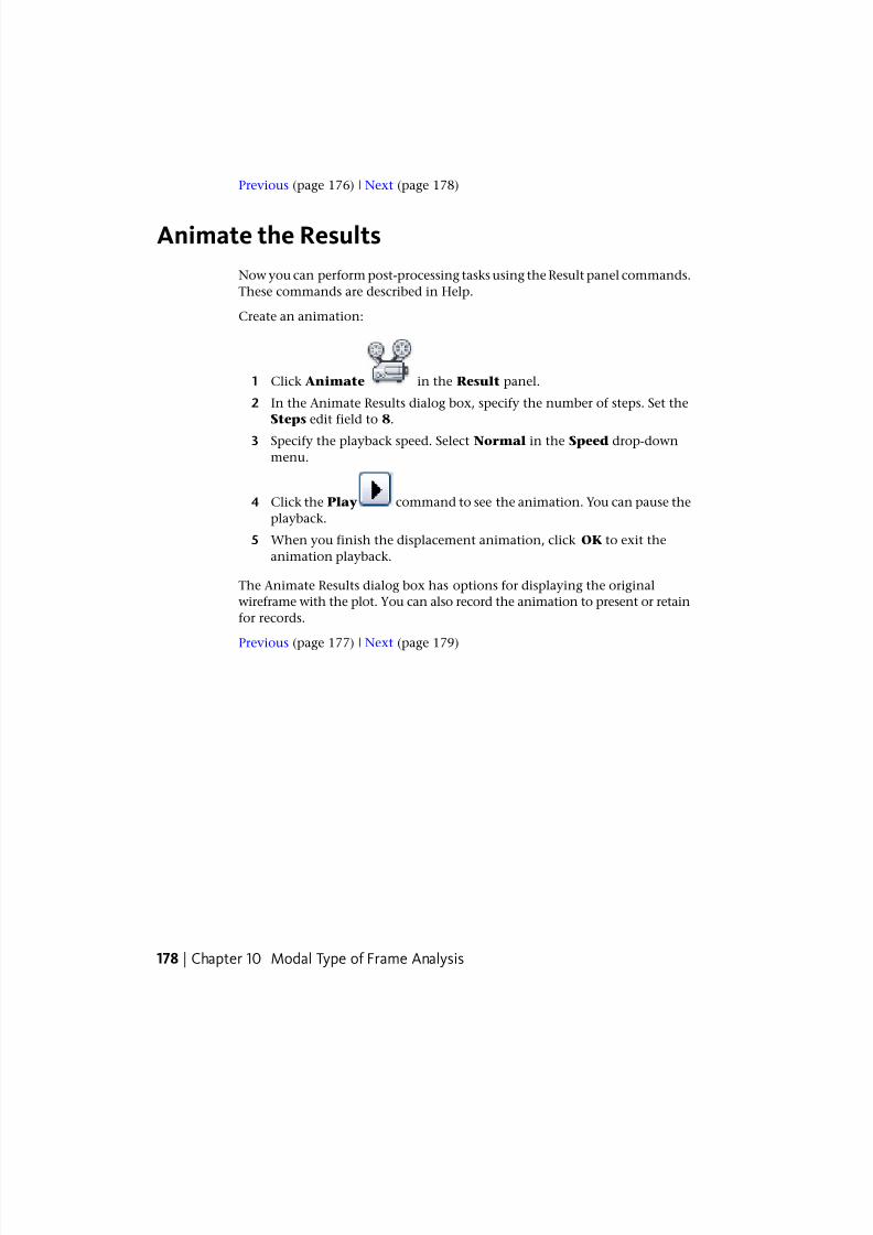
8/20/2019 Stress Analysis INVENTOR
http://slidepdf.com/reader/full/stress-analysis-inventor 184/266
Previous (page 176) | Next (page 178)
Animate the Results
Now you can perform post-processing tasks using the Result panel commands.
These commands are described in Help.
Create an animation:
1 Click Animate in the Result panel.
2 In the Animate Results dialog box, specify the number of steps. Set the
Steps edit field to 8.
3 Specify the playback speed. Select Normal in the Speed drop-down
menu.
4 Click the Play command to see the animation. You can pause the
playback.
5 When you finish the displacement animation, click OK to exit the
animation playback.
The Animate Results dialog box has options for displaying the original
wireframe with the plot. You can also record the animation to present or retain
for records.
Previous (page 177) | Next (page 179)
178 | Chapter 10 Modal Type of Frame Analysis

8/20/2019 Stress Analysis INVENTOR
http://slidepdf.com/reader/full/stress-analysis-inventor 185/266
Summary
In this tutorial, you performed a structural frequency (modal analysis) analysis
with the goal of finding natural mode shapes and frequencies of vibration.
The steps performed include:
■ Create a modal simulation.
■ Change simulation properties.
■ Exclude components from simulation.
■ Run a simulation.
■ View the results.
■ Create an animation of results.
Previous (page 178)
Summary | 179

8/20/2019 Stress Analysis INVENTOR
http://slidepdf.com/reader/full/stress-analysis-inventor 186/266
180

8/20/2019 Stress Analysis INVENTOR
http://slidepdf.com/reader/full/stress-analysis-inventor 187/266
Dynamic Simulation -Part 1
About this tutorialSimulate and analyze the dynamic characteristics of an assembly in motion
under various load conditions.
SimulationCategory
40 minutesTime Required
Reciprocating Saw.iamTutorial File Used
NOTE Click and read the required Tutorial Files Installation Instructions atht-
tp://www.autodesk.com/inventor-tutorial-data-sets . Then download the tutorial datasets and the required Tutorial Files Installation Instructions, and install the datasets
as instructed.
Dynamic Simulation contains a wide range of functionality and accommodates
numerous workflows. This tutorial helps you become familiar with the key
paradigms and features of Dynamic Simulation. Then you can explore other
capabilities, and apply Dynamic Simulation to your particular needs.
Objectives
■ Recognize the differences between the Dynamic Simulation application and
the regular assembly environment.
■ See how the software automatically converts mate assembly constraints to
Dynamic Simulation standard joints.
11
181

8/20/2019 Stress Analysis INVENTOR
http://slidepdf.com/reader/full/stress-analysis-inventor 188/266

8/20/2019 Stress Analysis INVENTOR
http://slidepdf.com/reader/full/stress-analysis-inventor 189/266
3 Click➤
Save As. Use RecipSaw-tutorial_1.iam for thename.
4 Click Save.
As you work through the following exercises, save this assembly periodically.
Previous (page 181) | Next (page 183)
Degrees of Freedom
Before going further in the tutorial, it is good to understand the differences
between the assembly modeling and dynamic simulation environments.
Though both environments have to do with creating mechanisms, there aresome critical differences between Dynamic Simulation and the Assembly
environment. The basic difference has to do with degrees of freedom and how
they are managed.
In the assembly environment, unconstrained and ungrounded components
have six degrees of freedom.
You add constraints to restrict degrees of freedom. For example, adding one
flush constraint between this part and one of its canonical planes removes 3
degrees of freedom.
Degrees of Freedom | 183
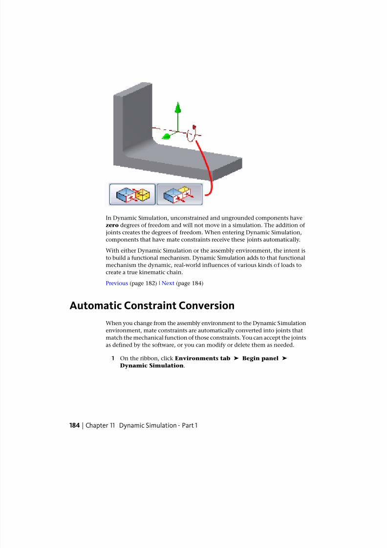
8/20/2019 Stress Analysis INVENTOR
http://slidepdf.com/reader/full/stress-analysis-inventor 190/266
In Dynamic Simulation, unconstrained and ungrounded components have
zero degrees of freedom and will not move in a simulation. The addition of
joints creates the degrees of freedom. When entering Dynamic Simulation,
components that have mate constraints receive these joints automatically.
With either Dynamic Simulation or the assembly environment, the intent is
to build a functional mechanism. Dynamic Simulation adds to that functional
mechanism the dynamic, real-world influences of various kinds of loads to
create a true kinematic chain.
Previous (page 182) | Next (page 184)
Automatic Constraint Conversion
When you change from the assembly environment to the Dynamic Simulation
environment, mate constraints are automatically converted into joints that
match the mechanical function of those constraints. You can accept the joints
as defined by the software, or you can modify or delete them as needed.
1 On the ribbon, click Environments tab ➤
Begin panel ➤
Dynamic Simulation.
184 | Chapter 11 Dynamic Simulation - Part 1

8/20/2019 Stress Analysis INVENTOR
http://slidepdf.com/reader/full/stress-analysis-inventor 191/266
NOTE If you are prompted to run the Dynamic Simulation Tutorial, click
No.
The Dynamic Simulation environment is active. You will notice that the
browser and its nodes have changed for the simulation environment.
In the simulation browser there are several folders for simulation objects.
They relate to the simulation as follows:
Components with no degrees of freedomGrounded folder
Components with degrees of freedom allowing them to participate in
the simulation when forces are applied.
Each mobile group is assigned a specific color. Right-click the Mobile
Groups folder and click Color Mobile Groups to visually determine mobile
groups the component resides in.
Mobile Groups folder
Joints created by automatic constraint conversion when entering thedynamic simulation environment. Contributing constraints are displayed
as child nodes.
Standard Joints folder
All non-standard joints that are created reside in folders for those specific
joint types. Contributing constraints are displayed as child nodes.
Various Joint folders
Loads that you define, including Gravity, are displayed in this folder.External Loads folder
NOTE Assemblies containing legacy, pre-Inventor 2008, Dynamic Simulation
objects DO NOT have their constraints automatically converted upon entering
the simulation environment.
2 Expand the Standard Joints folder.
Automatic Constraint Conversion | 185

8/20/2019 Stress Analysis INVENTOR
http://slidepdf.com/reader/full/stress-analysis-inventor 192/266
These joints were automatically created based on the assembly constraint
scheme. The software analyzes mate constraints and determines which
joint will best equate with the constraint scheme.
You can disable the automatic conversion of constraints, and then
manually convert only those you want in the simulation. Note, however,
that when you turn off automatic constraint conversion, all existing
joints are deleted, including manually created joints, thereby removing
all degrees of freedom.
To disable automatic constraint conversion, click Dynamic Simulation
tab ➤
Manage panel ➤
Simulation Settings. Clear the
check mark next to Automatically Convert Constraints to
Standard Joints so that this option is no longer active. Click Yes,
when prompted, then click OK on the dialog box. All joints in the
assembly are deleted.
To turn automatic constraint conversion back on, click the Simulation
Settings command and check the Automatically Convert
Constraints to Standard Joints option.
3 Click OK. Standard joints are created.
NOTE If you previously created non-standard joints in this assembly, these
joints are deleted.
4 Expand the Mobile Groups folder.
Components whose constraint scheme displays controlled motion haverelationships built and are grouped based on the relationship.
5 Expand the Welded Group folder.
Where a rigid relationship exists between components the software may
create a welded group. There are no degrees of freedom between the
members of a welded group.
6 Right-click the Mobile Groups folder, and click Color mobile groups.
All members within a group are assigned a color by the software. This
feature is used to easily identify members of a mobile group.
7 Right-click the Mobile Groups folder and click Color mobile groups
again to turn off the group coloring.
Previous (page 183) | Next (page 187)
186 | Chapter 11 Dynamic Simulation - Part 1

8/20/2019 Stress Analysis INVENTOR
http://slidepdf.com/reader/full/stress-analysis-inventor 193/266

8/20/2019 Stress Analysis INVENTOR
http://slidepdf.com/reader/full/stress-analysis-inventor 194/266

8/20/2019 Stress Analysis INVENTOR
http://slidepdf.com/reader/full/stress-analysis-inventor 195/266
Add a Rolling Joint
Now we need to build the relationship between the bevel gears.
There are two bevel gears, a larger one associated with the cam action, and a
smaller one associated with the motor assembly. We will work with the smaller
gear to start with.
1 Expand the Mobile Groups folder and Motor node to reveal the Bevel
Gear1 node.
2 Right-click the Bevel Gear node and click Edit.
You are automatically placed in the Part editing environment.
3 In the browser, expand the Surface Bodies(1) folder.
4 Right-click the Srf1 browser node, and click Visibility.
We will use the surface to help define the bevel gear relationship.
5 On the ribbon, click Return to go back to the simulation
environment. Alternatively, right-click in the graphic area, and click
Finish Edit.
6 On the ribbon, click Dynamic Simulation tab ➤
Joint panel ➤
Insert Joint to display the Insert Joint dialog box.
7 In the drop-down list, select Rolling: Cone on Cone.
Add a Rolling Joint | 189

8/20/2019 Stress Analysis INVENTOR
http://slidepdf.com/reader/full/stress-analysis-inventor 196/266
8 The component selector is automatically active, allowing you
to begin selection. Select the Pitch diameter circle at the base of the
surface cone.
9 Click the component 2 selector , and select a conical face
on Bevel Gear2.
You may have to expand the Mobile Groups and Cam crank browser
nodes to see the second gear.
10 Click OK.
11 Click and drag the motor bevel gear. The Cam crank assembly moves
because of the joint you created.
12 Edit the part again, and turn off Visibility of the Srf1 surface body.
Previous (page 187) | Next (page 190)
Building a 2D Contact
The next relationship that needs to be built is one between the cam Follower
Roller and the cam component. The Follower Roller needs to contact the cam.
190 | Chapter 11 Dynamic Simulation - Part 1

8/20/2019 Stress Analysis INVENTOR
http://slidepdf.com/reader/full/stress-analysis-inventor 197/266
Retaining degrees of freedom
The Follower Roller is a symmetrical part and, by default, dynamic simulationattempts to reduce symmetrical component movement. Why? An example
will help.
Consider a wheel assembly. You have a tire mounted to a rim. That assembly
is attached to the vehicle with lug nuts.The function of a lug nut, for
simulation purposes, isn’t to revolve around its axis; it is to constrain the
assembly to the vehicle. Because the lug nut is a symmetrical component, the
rotational degree of freedom (DOF) is automatically removed. This simplifies
the model for simulation purposes. If you want to retain the lug nut’s rotational
DOF, you can do so using the Retain DOF command. The same is true in
reverse. That is, you can use Ignore DOF to restrict the degrees of freedom
of a component.
To ensure that the Follower Roller contacts the cam while also keeping its
degree of freedom:
1 In the Mobile Groups folder, expand the Welded group. There are
two components in the group.
2 Right-click the Follower Roller component, and click Retain DOF.
The roller retains its motion characteristics. Now, we need to make sure
the roller contacts the cam.
3 Click the Insert Joint command to display the dialog box. From the
list, select 2D Contact.
4 Select the cam profile edge.
5 Select the sketch profile displayed on the roller component. As you can
see, you can use sketch geometry as part of the simulation.
Building a 2D Contact | 191

8/20/2019 Stress Analysis INVENTOR
http://slidepdf.com/reader/full/stress-analysis-inventor 198/266
6 Click OK.
7 Drag the Follower until it contacts the cam. It makes contact but does
not penetrate the cam. The 2D contact established a mechanical
relationship between the two components.
Before going any further, we will modify the properties of the 2D contact
and display the force vector.
8 In the browser, right-click the 2D contact joint, and click Properties.
192 | Chapter 11 Dynamic Simulation - Part 1

8/20/2019 Stress Analysis INVENTOR
http://slidepdf.com/reader/full/stress-analysis-inventor 199/266
9 Set the Restitution value to 0.0, and Friction to 0.15.
10 Expand the dialog box to access the lower section. Check the
Normal box, and set the Scale to 0.003.
11 Click OK.
Previous (page 189) | Next (page 193)
Add Spring, Damper, and Jack Joint
The Follower is designed to slide through a portion of the Guide component.However, to hold the Follower Roller against the Cam, we must specify a
Add Spring, Damper, and Jack Joint | 193

8/20/2019 Stress Analysis INVENTOR
http://slidepdf.com/reader/full/stress-analysis-inventor 200/266
spring between the Follower and Guide components. Dynamic Simulation
offers a joint for doing that and more - the Spring/Damper/Jack joint.
Depending on the joint type, the dialog box provides applicable inputs to
help define the joint.
1 Click the Insert Joint command and in the dialog box, select Spring
/ Damper / Jack from the drop-down list of joint types. The
Component 1 selector is active.
2 On the Guide component, select the hole profile where the Follower
passes through the Guide.This creates one contact for the spring.
3 Select the edge profile where the spring will contact the follower.
4 Click OK.
The result is a spring joint in the browser and a graphic representation
of a spring. The representation is deformable and has action-reaction
forces, but does not have mass.
194 | Chapter 11 Dynamic Simulation - Part 1
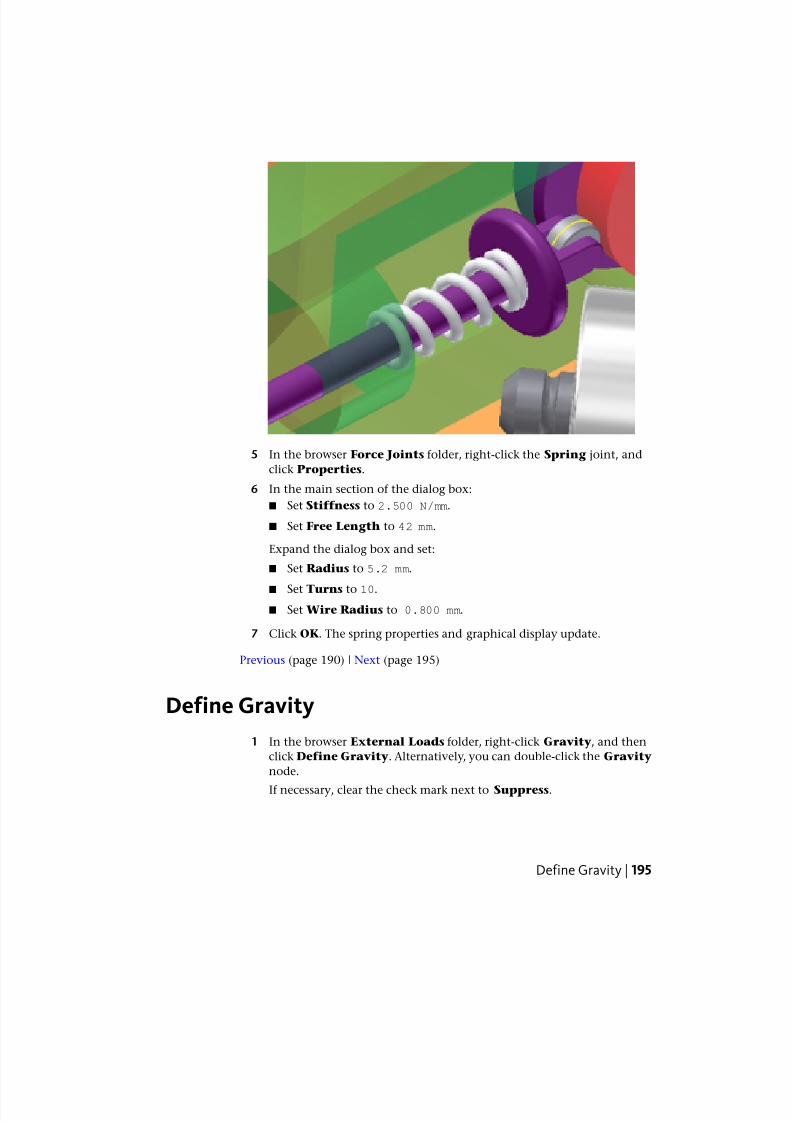
8/20/2019 Stress Analysis INVENTOR
http://slidepdf.com/reader/full/stress-analysis-inventor 201/266
5 In the browser Force Joints folder, right-click the Spring joint, and
click Properties.
6 In the main section of the dialog box:
■ Set Stiffness to 2.500 N/mm.
■ Set Free Length to 42 mm.
Expand the dialog box and set:
■ Set Radius to 5.2 mm.
■ Set Turns to 10.
■ Set Wire Radius to 0.800 mm.
7 Click OK. The spring properties and graphical display update.
Previous (page 190) | Next (page 195)
Define Gravity
1 In the browser External Loads folder, right-click Gravity, and then
click Define Gravity. Alternatively, you can double-click the Gravity
node.
If necessary, clear the check mark next to Suppress.
Define Gravity | 195

8/20/2019 Stress Analysis INVENTOR
http://slidepdf.com/reader/full/stress-analysis-inventor 202/266
2 Select the Case edge as shown in the image to specify a vector for gravity.
You can use the Invert or Reverse command to change
directions.
3 Click OK.
Note that the direction of gravity has nothing to do with any external
notion of "up" or "down," but is set according to the vector you specify.
Previous (page 193) | Next (page 196)
Impose Motion on a Joint
To simulate saw operation, it is necessary to impose motion. In this case, we
will apply motion to the motor, just as would be the real world case. To impose
motion, you must edit the joint properties.
1 In the browser Standard Joints folder, right-click the Revolution:2
(Saw layout:1. Motor:1) joint, and click Properties.
196 | Chapter 11 Dynamic Simulation - Part 1

8/20/2019 Stress Analysis INVENTOR
http://slidepdf.com/reader/full/stress-analysis-inventor 203/266
2 Click the dof 1 (R) tab.
3 Click the Edit imposed motion command , and check
Enable imposed motion.
4 Click the arrow to expand the input choices, and click Constant Value.
Specify 10000 deg/s (ten thousand).
5 Click OK.
Previous (page 195) | Next (page 197)
Run a Simulation
Because the simulation is of a high speed device, we will modify the simulation
properties.
1 On the Simulation Player in the Final Time field, enter .5 s, which
is sufficient to demonstrate the mechanism.
TIP Use the tooltips to see the names of the fields on the Simulation Player.
NOTE The software automatically increases the value in the Images fieldproportionally to the change in the Final Time field. Press the Tab key
to move the cursor out of the Final Time field and update the Images
field.
2 In the Images field, enter 200. Increasing the image count improves
the results we will view in the Output Grapher.
3 Click Run on the Simulation Player.
Run a Simulation | 197

8/20/2019 Stress Analysis INVENTOR
http://slidepdf.com/reader/full/stress-analysis-inventor 204/266
As the Motor component drives the bevel gear, the remaining parts in
the kinematic chain respond.
Also, because we have not yet specified any frictional or damping forces,
the mechanism is lossless. There is no friction between components,
regardless of how long the simulation runs.
4 If the simulation is still running, click Stop on the Simulation Player.
Before leaving the simulation run environment, we’ll take a look at the Output
Grapher.
Previous (page 196) | Next (page 198)
Using the Output Grapher
The Output Grapher is the means to examine a variety of results from thesimulation. The following list describes some of the things you can do after
running a simulation:
■ Change reference frames to view results in various coordinate systems.
■ Display curve results.
■ Save the simulation results for later review and comparison.
■ Display results in terms of time or other criteria.
1 After running the simulation, but before leaving the run environment,
on the ribbon click Dynamic Simulation tab ➤
Results panel ➤
Output Grapher .
The Output Grapher is divided into different sections: browser, graph,
and time steps. Commands specific to Output Grapher are located on a
toolbar across the top of the window. The window is resizable, so adjust
it to meet your needs.
2 In the browser of the Dynamic Simulation - Output Grapher window,
expand the Standard Joints node. Then, expand the Revolution:2
node.
3 Under the Revolution:2 node, expand the Driving force node. Check
the box next to U_imposed[1]. You will see the force displayed in the
graph region.
4 Expand the Prismatic:3 node.
198 | Chapter 11 Dynamic Simulation - Part 1

8/20/2019 Stress Analysis INVENTOR
http://slidepdf.com/reader/full/stress-analysis-inventor 205/266
5 Expand the Velocities node, and check V[1]. The velocity is presented
in the graph with the driving force.
6 Close the Output Grapher window.
Previous (page 197) | Next (page 199)
Simulation Player
Let's take a quick look at some features on the Simulation Player.
As mentioned, the Final Time field controls the total time available for a
simulation.
Simulation Player | 199

8/20/2019 Stress Analysis INVENTOR
http://slidepdf.com/reader/full/stress-analysis-inventor 206/266
The Images field controls the number of image frames available for a
simulation. Click Construction Mode , change this value to 100, andrun the simulation. Click Construction Mode when the simulation is
finished and change this value back to 200.
The Filter field controls the frame display step. If the value is set to 1, all
frames play. If the value is set to 5, only every fifth frame displays, and so on.
This field is editable when simulation mode is active, but not while a
simulation is running.
The Simulation Time value shows the duration of the motion of the
mechanism as would be witnessed with the physical model.
200 | Chapter 11 Dynamic Simulation - Part 1

8/20/2019 Stress Analysis INVENTOR
http://slidepdf.com/reader/full/stress-analysis-inventor 207/266
The Percent value shows the percent complete of a simulation.
The Real Time of Computation value shows the actual time it takes to
run the simulation. This is affected by the complexity of the model and your
computer's resources.
You can click Screen Refresh to turn off screen refresh during the
simulation. The simulation runs, but there is no graphic representation.
Simulation Player | 201

8/20/2019 Stress Analysis INVENTOR
http://slidepdf.com/reader/full/stress-analysis-inventor 208/266
Click the Construction Mode command to exit the simulation runenvironment. The construction mode is where you create and edit joints.
IMPORTANT Save the assembly before exiting. This will enable you to go to the
next tutorial and use this assembly as the basis for that tutorial.
Previous (page 198) | Next (page 202)
Summary
You can also export load conditions at any simulation motion state to Stress
Analysis. In Stress Analysis, you can see, from a structural point of view, howparts respond to dynamic loads at any point in the assembly's range of motion.
In this tutorial, the skills you learned include:
■ Understanding basic differences between the Dynamic Simulation
application and the regular assembly environment.
■ Having the software automatically convert relevant assembly constraints
to Dynamic Simulation standard joints.
■ Use Color Mobile Groups to distinguish component relationships.
■ Manually creating rolling, 2D contact, and Spring joint types.
■ Defining joint properties.
■ Imposing motion on a joint and defining gravity.
■ Using Output graphers.
202 | Chapter 11 Dynamic Simulation - Part 1

8/20/2019 Stress Analysis INVENTOR
http://slidepdf.com/reader/full/stress-analysis-inventor 209/266
■ Running a dynamic simulation to see how joints, loads, and component
structures interact as a moving, dynamic mechanism.
Remember to check the Help files for further information. And, remember to
go online at autodesk.com for more tutorials and Skill Builders.
Previous (page 199)
Summary | 203

8/20/2019 Stress Analysis INVENTOR
http://slidepdf.com/reader/full/stress-analysis-inventor 210/266
204

8/20/2019 Stress Analysis INVENTOR
http://slidepdf.com/reader/full/stress-analysis-inventor 211/266
Dynamic Simulation -Part 2
About this tutorial
Add the blade assembly and complete the operating conditions definition,
modify the cam lobe, and then publish the simulation with Inventor Studio.
SimulationCategory
20 minutesTime Required
Used in the tutorial:Tutorial Files Used
RecipSaw_tutorial_1.iamBlade set.iam
12
205

8/20/2019 Stress Analysis INVENTOR
http://slidepdf.com/reader/full/stress-analysis-inventor 212/266
Completed file:
Reciprocating Saw FINAL.iam
NOTE Click and read the required Tutorial Files Installation Instructions atht-
tp://www.autodesk.com/inventor-tutorial-data-sets . Then download the tutorial
data sets and the required Tutorial Files Installation Instructions, and install the
datasets as instructed.
In this tutorial, we pick up where we left off in the Dynamic Simulation
Fundamentals - Part 1 tutorial.
Objectives
■ Add the saw blade subassembly.
■ Add various joints.
■ Impose motion, friction, and retain degrees of freedom in subassemblies.
■ Add traces.
■ Publish a simulation animation using Inventor Studio.
Prerequisites
■ Complete the Dynamic Simulation Fundamentals - Part 1 tutorial.
■ Complete the Studio - Animations tutorial.
■ Understand the basics of motion.
■ See the Help topic “Getting Started” for further information.
Navigation Tips
■ Use Next or Previous at the bottom-left to advance to the next page orreturn to the previous one.
Next (page 206)
Work in the Simulation Environment
Understanding Simulation Commands
Large and complex moving assemblies coupled with hundreds of articulated
moving parts can be simulated. The Autodesk Inventor Simulation provides:
■ Interactive, simultaneous, and associative visualization of 3D animations
with trajectories; velocity, acceleration, and force vectors; and“deformable
”
springs.
206 | Chapter 12 Dynamic Simulation - Part 2

8/20/2019 Stress Analysis INVENTOR
http://slidepdf.com/reader/full/stress-analysis-inventor 213/266
■ Graphic generation command for representing and post-processing the
simulation output data.
Simulation Assumptions
The dynamic simulation commands provided in Autodesk Inventor Simulation
help in the steps of conception and development and in reducing the number
of prototypes. However, due to the hypothesis used in the simulation, it only
provides an approximation of the behavior seen in real-life mechanisms.
Interpreting Simulation Results
To avoid computations that can lead to a misinterpretation of the results or
incomplete models that cause unusual behavior, or even make the simulation
impossible to compute, be aware of the rules that apply to:
■ Relative parameters
■ Coherent masses and inertia
■ Continuity of laws
Relative Parameters
The Autodesk Inventor Simulation uses relative parameters. For example, the
position variables, velocity, and acceleration give a direct description of the
motion of a child part according to a parent part through the degree of freedom
(DOF) of the joint that links them. As a result, select the initial velocity of a
degree of freedom carefully.
Coherent Masses and Inertia
Ensure that the mechanism is well-conditioned. For example, the mass and
inertia of the mechanism should be in the same order of magnitude. The mostcommon error is a bad definition of density or volume of the CAD parts.
Continuity of Laws
Numerical computing is sensitive toward discontinuities in imposed laws.
While a velocity law defines a series of linear ramps, the acceleration is
necessarily discontinuous. Similarly, when using contact joints, it is better to
avoid profiles or outlines with straight edges.
NOTE Using little fillets eases the computation by breaking the edge.
Previous (page 205) | Next (page 208)
Work in the Simulation Environment | 207

8/20/2019 Stress Analysis INVENTOR
http://slidepdf.com/reader/full/stress-analysis-inventor 214/266
Construct the Operating Conditions
We will now complete the motion definitions so that the simulation reflects
product operating conditions.
If the RecipSaw-tutorial_1.iam assembly is not open, open the file to continue.
As you can see, although we have the saw body, we do not have the blade
components. To add the blade components it is not necessary to leave the
simulation environment.
NOTE Make sure you are in Construction Mode before performing the next steps.
1 Click the Assemble tab to display the Assembly ribbon.
2 In the Component panel, click Place Component. Select Dynamic
Simulation 1 and 2
➤
Blade set.iam and click Open.
3 Position the Blade set assembly near where it will be assembled.
4 Right-click in the graphics window, and click Done.
5 In the browser, expand the Blade set assembly node to display the
components.
208 | Chapter 12 Dynamic Simulation - Part 2
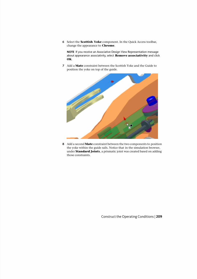
8/20/2019 Stress Analysis INVENTOR
http://slidepdf.com/reader/full/stress-analysis-inventor 215/266
6 Select the Scottish Yoke component. In the Quick Access toolbar,
change the appearance to Chrome.
NOTE If you receive an Associative Design View Representation message
about appearance associativity, select Remove associativity and click
OK.
7 Add a Mate constraint between the Scottish Yoke and the Guide to
position the yoke on top of the guide.
8 Add a second Mate constraint between the two components to position
the yoke within the guide rails. Notice that in the simulation browser,under Standard Joints, a prismatic joint was created based on adding
those constraints.
Construct the Operating Conditions | 209

8/20/2019 Stress Analysis INVENTOR
http://slidepdf.com/reader/full/stress-analysis-inventor 216/266
Previous (page 206) | Next (page 210)
Add Friction
The mechanism thus far is lossless; meaning that it operates without friction
or dampening as would normally be experienced. We will now add friction
to capture the operating environment.
Add Friction and complete the yoke-guide relationship
1 In the browser, right-click Blade set.iam, and click Flexible. By setting
the assembly to Flexible, the assembly is placed into the welded group
folder. Within that assembly, the constraints are evaluated and the
constraint between the yoke and blade causes the addition of aRevolution joint.
210 | Chapter 12 Dynamic Simulation - Part 2

8/20/2019 Stress Analysis INVENTOR
http://slidepdf.com/reader/full/stress-analysis-inventor 217/266
2 As previously mentioned, the assembly has no friction yet. This step
imposes friction on the prismatic joint. Right-click the Prismatic Joint
for the Guide and the Scottish Yoke, and click Properties.
3 Click the dof 1 (T) tab.
4 Click the Edit joint force command .
5 Click Enable joint force.
6 Enter a Dry Friction coefficient of 0.1, and click OK.7 Now, you must add a constraint to position the Scottish Yoke with respect
to the crank assembly. First, set the browser view to Model, and expand
the Blade set.iam node.
8 Expand the Scottish Yoke node, and click the Constrain command.
9 In the browser, select Work Plane3 under the Scottish Yoke
component.
10 In the graphics window, select a circular edge of the Roller component
that is part of the Crank cam assembly. A Point-Plane joint is added to
reflect the constraint.
Add Friction | 211

8/20/2019 Stress Analysis INVENTOR
http://slidepdf.com/reader/full/stress-analysis-inventor 218/266
11 Click OK to add the constraint and close the dialog box.
12 Set the browser view back to Dynamic Simulation.
The resulting Point-Plane joint has five degrees of freedom and one constraint.
It is enough definition to transfer motion without over constraining the model.
Dynamic Simulation detects over-constrained conditions and helps you to
resolve them.
Previous (page 208) | Next (page 212)
Add a Sliding JointThe interface between the Blade set and the saw drivetrain is not yet completely
defined. We must have the follower end interact with the Blade Clamp
component. It requires a sliding joint.
1 The next joint to add is the one between the Blade Clamp and the
Follower, so that the Follower travels in the blade clamp. If the Dynamic
Simulation tab is not active, select it.
2 Before creating the joint, it helps to lock the Prismatic Joint between the
Guide and Follower components. This prevents the related components
from moving and lets the solver work more efficiently.
Right-click the Prismatic:3 (Guide:1, Follower:1) joint, and click
Lock dofs.
212 | Chapter 12 Dynamic Simulation - Part 2

8/20/2019 Stress Analysis INVENTOR
http://slidepdf.com/reader/full/stress-analysis-inventor 219/266
3 Add the sliding joint. To do this, click Insert Joint. In the drop-down
list, select Sliding: Cylinder Curve. For input 1, select the blade clamp
slot profile on which the Follower rides.
4 For input 2, select the Follower cylinder face that rides in the slot.
Click OK.
5 Unlock the Prismatic Joint.
That completes this section on adding components and joints to the assembly.
In this section, you learned about:
■ Adding assembly components while in the simulation environment.
■ Adding assembly constraints and seeing them automatically create standard
joints.
■ Adding joints to simulate mechanical conditions within the assembly.
Previous (page 210) | Next (page 213)
Use the Input Grapher
The Input Grapher provides a means of adding forces and torques that change
during the simulation based on other independent variables.
Use the Input Grapher | 213

8/20/2019 Stress Analysis INVENTOR
http://slidepdf.com/reader/full/stress-analysis-inventor 220/266
We will add an external force that is dependent on the velocity in the prismatic
joint between the Guide and Scottish Yoke. To provide a sense of the velocity
we use + or - values to define an opposite force.
1 In the browser, in Standard Joints, select the joint Prismatic
(Guide:1, Scottish Yoke:1). Note that in the reference frames, when
the velocity is positive, the reference frames point away from the blade
end. If the reference frames point toward the saw blade, you may have
to edit the joint to reverse the direction.
2 In the Load panel, click the Force command. Select a vertex of one of
the saw teeth.
214 | Chapter 12 Dynamic Simulation - Part 2
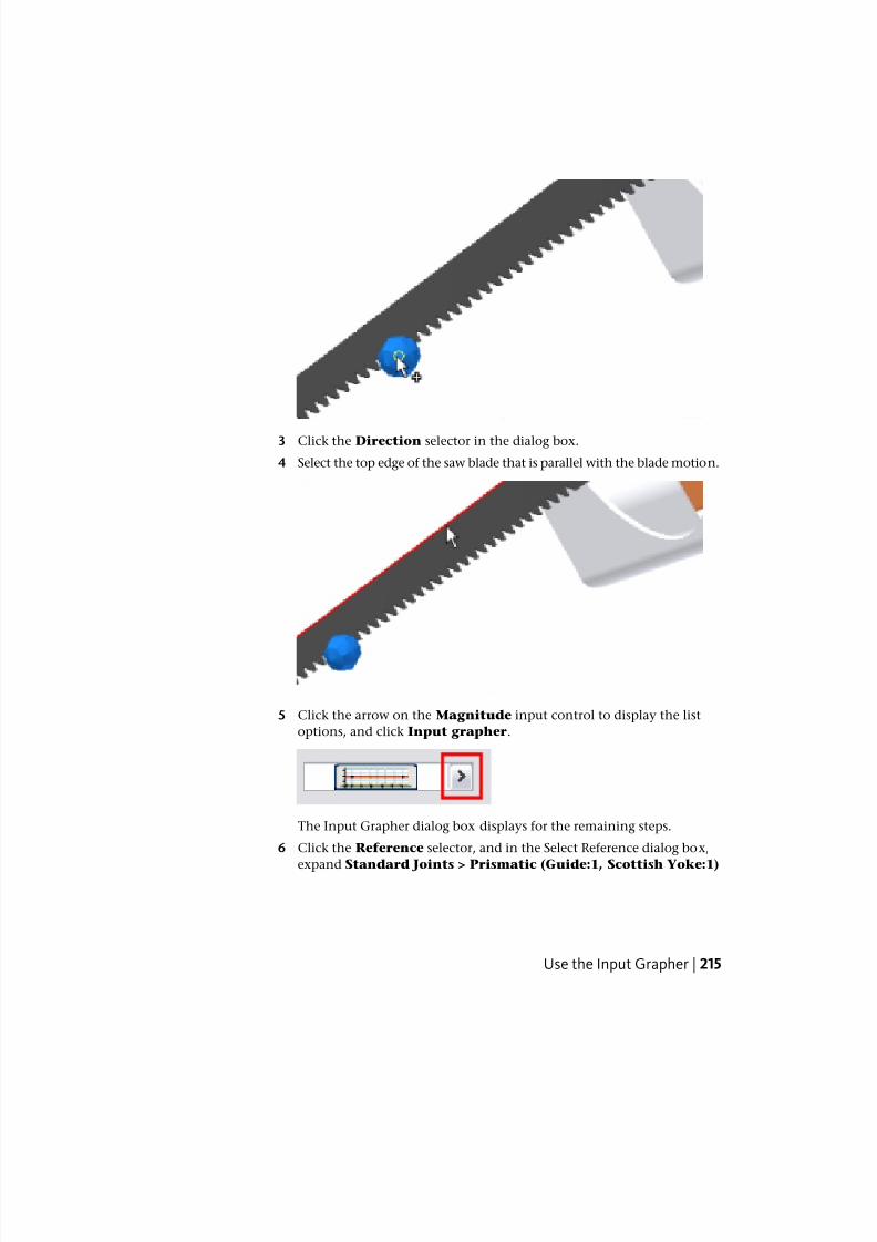
8/20/2019 Stress Analysis INVENTOR
http://slidepdf.com/reader/full/stress-analysis-inventor 221/266
3 Click the Direction selector in the dialog box.
4 Select the top edge of the saw blade that is parallel with the blade motion.
5 Click the arrow on the Magnitude input control to display the list
options, and click Input grapher.
The Input Grapher dialog box displays for the remaining steps.
6 Click the Reference selector, and in the Select Reference dialog box,
expand Standard Joints > Prismatic (Guide:1, Scottish Yoke:1)
Use the Input Grapher | 215

8/20/2019 Stress Analysis INVENTOR
http://slidepdf.com/reader/full/stress-analysis-inventor 222/266
to reveal the Velocities folder and contents. Click V(1) to specify velocity
as variable for the graph X axis.
7 Click OK. Notice in the graph region the X axis of the graph shows the
reference you just specified.
When navigating inside the graph region.
■
You can roll the mouse wheel, if you have one, to zoom in and out.
■ To Pan the graph, click and drag the middle mouse button or wheel
and watch the cursor move around the graph region.
216 | Chapter 12 Dynamic Simulation - Part 2

8/20/2019 Stress Analysis INVENTOR
http://slidepdf.com/reader/full/stress-analysis-inventor 223/266
8 In the lower section of the Input Grapher, for the Starting Point
section, set X1 = -10 mm/s and Y1 = 250 N.
9 In the Ending Point section, set X2 = -0.1 mm/s and Y2 = 250 N.
10 Double-click in the graph area to the right and below the second point.
This adds a new point, effectively creating a section in the graph.
NOTE You can also right-click beyond the second point and click AddPoint to start a new section. To select the second section, click on the line
between the points.
11 The Starting Point for the second section (X1, Y1) is the previous
section end point and is already set. To specify the second section
Ending Point, set X2 = 0.0 mm/s and set Y2 = -250 N.
12 Add a third section to the right of the second section. To specify the
third section Ending Point, set X2 = 10.0 mm/s and Y2 = -250 N.
13 Click OK to close the Input Grapher.
14 Expand the dialog box and check the Display option at the bottom.
You can also specify a different color to differentiate the force visually.
15 Click OK to accept the input and close the Force dialog box.
16 Run the simulation. Do not leave the Run environment.
Previous (page 212) | Next (page 217)
Use the Output Grapher
The Output Grapher allows you to examine various results from the simulation.
The following is a list of some of the things you can do after running a
simulation:
■ Display vectors for internal or external forces.
■ Change reference frames to view results in various coordinate systems.
Use the Output Grapher | 217

8/20/2019 Stress Analysis INVENTOR
http://slidepdf.com/reader/full/stress-analysis-inventor 224/266
■ Display curve results.
■ Save the simulation results for later review and comparison.
■ Display results in terms of time or other criteria.
■ Display traces to visualize trajectory of component points.
Display Traces
1 After running the simulation, and before leaving the run environment,
click the Output Grapher command.
The Output Grapher window is divided into different sections: browser,
graph, and time steps. Output Grapher commands are located in a toolbar
across the top of the window. The window is resizable, so adjust it to
meet your needs.
2 Click Add Trace . The dialog box displays, and the Origin selector
is actively awaiting an input. Select the point at the end of the saw blade.
3 In the dialog box, check the Output trace value option and click
Apply.
4 Add two additional trace points along the saw blade in the same manner,
and be sure to export the trace for each point.
218 | Chapter 12 Dynamic Simulation - Part 2
8/20/2019 Stress Analysis INVENTOR
http://slidepdf.com/reader/full/stress-analysis-inventor 225/266
5 Close the dialog box.
Set Trace as Reference
1 In the Output Grapher browser, expand Traces.
2 Expand Trace:1, and then Positions.
3 Right-click P[X], and click Set as Reference.
4 Use the Output Grapher Save command to save the Simulation.
5 Enter the name RecipSaw_tutorial_1.iam, and click Save.
6 In the grapher browser, right-click P[X] and uncheck Set as Reference.
7 Close the Output Grapher.
8 Click Construction Mode in the Simulation Player.
As you can see, you can save simulation data, make changes, and comparethe change results with the previous data.
Previous (page 213) | Next (page 219)
Export to FEA
Next we will export motion loads and run a stress simulation on a component.
Use the following process for every component you want to analyze in the
stress analysis environment.
Select the component
Use the following process for each component you want to analyze in FEA:
1 Run the simulation.
2 Open the Output Grapher.
3 In the Output Grapher toolbar, click Export to FEA.
4 In the simulation browser, select Follower:1 and click OK. The dialog
box for selecting load bearing inputs is displayed.
Select faces
Three joint inputs are required to satisfy the motion requirements for exporting
the Follower component.
1 In the graphics window, select the long shaft of the Follower component,which satisfies the prismatic joint input.
Export to FEA | 219

8/20/2019 Stress Analysis INVENTOR
http://slidepdf.com/reader/full/stress-analysis-inventor 226/266
2 In the dialog box, click Revolution 5.3 Select the small shaft that is used with the Follower Roller.
4 In the dialog box, click the Spring joint.
5 In the graphics window, click the face where the spring contacts the
follower, and click OK.
220 | Chapter 12 Dynamic Simulation - Part 2

8/20/2019 Stress Analysis INVENTOR
http://slidepdf.com/reader/full/stress-analysis-inventor 227/266
Next, specify the time steps to analyze:
1 Click the Deselect all command in the Output Grapher toolbar.2 Expand the Standard Joints, Revolution:5, and Force folders. Click
Force.
3 Expand the Force Joints, Spring / Damper / Jack joint, and Force
folders. Click Force.
4 In the graph region, double-click a Force (Revolution) graph high point
you want to analyze. In the time steps section above the graph, place a
check mark next to the corresponding time step.
Export to FEA | 221

8/20/2019 Stress Analysis INVENTOR
http://slidepdf.com/reader/full/stress-analysis-inventor 228/266
5 Using the same method, select a low point of the Force (Revolution)
values. Place a check mark next to its time step.
6 Close the Output Grapher.
Import into Autodesk Inventor Stress Analysis
1 Click Finish Dynamic Simulation.
2 On the Environments tab, click Stress Analysis to open in the Stress
Analysis environment.
3 In the Manage panel, click Create Simulation.
4 In the dialog box, under Static Analysis, select the Motion Loads
Analysis option. The two list controls below the option are enabled
and populated with the exported parts and time steps.
5 In the Part list, select the Follower component.
6 In the Time Step list, select a time step to analyze.
7 Click OK. The assembly updates to represent that time step and then
isolates the Follower component for analysis. You can observe symbols
representing the various forces acting on the Follower.
8 Click Mesh Settings, then click Create Curved Mesh Elements.
222 | Chapter 12 Dynamic Simulation - Part 2

8/20/2019 Stress Analysis INVENTOR
http://slidepdf.com/reader/full/stress-analysis-inventor 229/266
9 In the Solve panel, click Simulate, and then click Run. Wait for the
simulation to complete.
10 Select from the various Results data to see how the component performs
at that time step.
11 Click Finish Stress Analysis to exit the Stress Analysis environment.
Previous (page 217) | Next (page 223)
Publish Output in Inventor Studio
You can publish the simulation in Inventor Studio and produce high quality
video output containing lighting, shadows, backgrounds, and so on.
1 Reenter the Dynamic Simulation environment and run the simulation.
After running the simulation, do not leave the run environment.
2 In the Animate panel, click Publish to Studio.
Publish Output in Inventor Studio | 223
8/20/2019 Stress Analysis INVENTOR
http://slidepdf.com/reader/full/stress-analysis-inventor 230/266
3 In the Studio environment, set up the following for your simulation:
■ Camera position, type, and associated settings.
■ Lighting style and its associated settings.
■ Scene style and its associated settings.
■ Different appearances, if desired.
If you are not experienced with Inventor Studio, take time to complete
a Studio tutorial to get familiar with the animation commands it provides.
Then, return to this part of the Dynamic Simulation tutorial and output
your simulation to Studio.
4 Click the Animation Timeline command to display the
timeline.
5 Set the timeline slider to the time at which the animation action is to
end, such as 2 seconds.
6 In the browser, expand the Animation Favorites folder. Right-click
the Simulation Timeline parameter, and click Animate Parameters
.
7 Set the Action End value to 200 ul.
8 Click OK.
9 In Studio, add lighting and scene styles as needed. Create the camera
angles you will use and complete the preparation of your animation.
NOTE If you have not used Inventor Studio to create animations previously,
you may want to do the rendering and animation tutorials, which cover the
information for this step.
10 Click the Render Animation command .
11 On the General tab, the styles you set up are the active ones. If not,
select them from the various lists.
12 On the Output tab, click the box next to Preview No Render. It
produces a test render for reviewing the animation action. Click OK to
render a preview.
224 | Chapter 12 Dynamic Simulation - Part 2

8/20/2019 Stress Analysis INVENTOR
http://slidepdf.com/reader/full/stress-analysis-inventor 231/266
13 Once you confirm the animation is playing like you want, cancel the
Preview option and render the simulation final animation with lighting
and scene styles. Click OK to render a realistic-looking simulation.
NOTE You may want to render images at a few different time positions to
ensure the lighting and scene styles look like you expect, then render the
animation.
14 Save the assembly.
Previous (page 219) | Next (page 225)
Summary
In this tutorial, we demonstrated a workflow to add components to an assemblywhile in the Dynamic Simulation environment. We added the blade assembly
and completed the operating conditions definition. Then we modified the
cam lobe, and finally published the simulation with Inventor Studio.
In this tutorial, you:
■ Added the saw blade subassembly.
■ Added various joints.
■ Imposed motion, friction, and retained degrees of freedom in subassemblies.
■ Added traces.
■ Published a simulation animation using Inventor Studio.
What Next? - As a next step, consider completing one of the following
tutorials:
■ Assembly Motion and Loads for a Cam and Lobe simulation
■ FEA using Motion Loads for exporting Motion Loads to stress analysis
■ Studio - Renderings for great looking images
■ Studio - Animations for creating animations of your product
Previous (page 223)
Summary | 225

8/20/2019 Stress Analysis INVENTOR
http://slidepdf.com/reader/full/stress-analysis-inventor 232/266
226

8/20/2019 Stress Analysis INVENTOR
http://slidepdf.com/reader/full/stress-analysis-inventor 233/266
Assembly Motion andLoads
About this tutorial
Simulate a cam and valve assembly.
SimulationCategory
13
227

8/20/2019 Stress Analysis INVENTOR
http://slidepdf.com/reader/full/stress-analysis-inventor 234/266
25 minutesTime Required
cam_valve.iamTutorial Files Used
NOTE Click and read the required Tutorial Files Installation Instructions atht-
tp://www.autodesk.com/inventor-tutorial-data-sets . Then download the tutorial
data sets and the required Tutorial Files Installation Instructions, and install the
datasets as instructed.
In this tutorial, you simulate a cam, valve, and spring mechanism. You
determine the contact forces between the cam and valve, the forces in the
spring, and the torque required to drive the cam.
In addition, you view the simulation results in the Output Grapher, and export
the simulation data to Microsoft Excel.
Objectives
■ Create a spring.
■ Create a 2D Contact joint.
■ Impose a motion.
■ Simulate dynamic motion.
■ View the simulation results.
■ Export the simulation results to Excel.
Prerequisites
■ It is recommended that you first complete the Dynamic Simulation
Fundamentals - Part 1 tutorial.
■ Understand the basics of motion and how it affects your design.
■ Know how to set the active project, navigate in model space with various
view commands, and perform common modeling functions such as
sketching and extruding.
■ See the Help topic, Getting Started, for more information.
Navigation Tips
■ Use Next or Previous at the bottom-left to advance to the next page or
return to the previous one.
Next (page 229)
228 | Chapter 13 Assembly Motion and Loads

8/20/2019 Stress Analysis INVENTOR
http://slidepdf.com/reader/full/stress-analysis-inventor 235/266
Open Assembly
To begin:
1 Set the active project to tutorial_files.
2 Open Dynamic Simulation 3 ➤
cam_valve.iam.
Open Assembly | 229

8/20/2019 Stress Analysis INVENTOR
http://slidepdf.com/reader/full/stress-analysis-inventor 236/266
3 Use Save As to save a copy of this file with the file name
cam_valve_tutorial.iam.
Previous (page 227) | Next (page 231)
230 | Chapter 13 Assembly Motion and Loads

8/20/2019 Stress Analysis INVENTOR
http://slidepdf.com/reader/full/stress-analysis-inventor 237/266
Activate Dynamic Simulation
1 On the ribbon, select Environments tab ➤
Begin panel ➤
Dynamic Simulation. The Dynamic Simulation tab displays in
place of the previous tab.
2 If you are prompted to run the Dynamic Simulation Tutorial, click No.
In the following pages, you specify the joints and forces necessary to
create a simulation.
Previous (page 229) | Next (page 231)
Automatic Joint Creation
By default, Dynamic Simulation automatically converts assembly constraints
to joints for assemblies created in the Autodesk Inventor 2008 or later releases.
The Dynamic Simulation browser lists two joints: a revolution joint between
the cam and the support, and a prismatic joint between the valve and the
support.
To complete the mechanism, you manually add a spring joint and a 2D contact
joint.
TIP Automatically created joints are maintained in the Standard Joints folder.
Joints that you add otherwise, reside in other folders based on the joint type.
TIP To delete automatically created joints, on the ribbon click Dynamic
Simulation tab ➤
Manage panel ➤
Simulation Settings, and then remove
the checkmark next to Automatically Convert Constraints to Standard
Joints. Click No, when prompted, and click OK or Apply in the dialog box.
Previous (page 231) | Next (page 232)
Activate Dynamic Simulation | 231

8/20/2019 Stress Analysis INVENTOR
http://slidepdf.com/reader/full/stress-analysis-inventor 238/266
Define Gravity
1 In the browser, under External loads, right-click Gravity, and then
select Define Gravity.
2 To define a vector for gravity, select one of the vertical edges of the
support.
Click the image to play the animation.
3 If the direction arrow points up, click Invert Normal to flip the
arrow.
4 Click OK.
5 Click Run on the Simulation Player. The valve responds to theforce of gravity and drops away from the mechanism.
6 On the Simulation Player, click Construction Mode .
Previous (page 231) | Next (page 232)
Insert a Spring
Before you insert the spring, make an adjustment to the mechanism.
1 If you have not already done so, you must return to the Construction
Mode. In the Simulation Player, click Construction Mode .
2 In the browser, right-click the prismatic joint, and then select
Properties.
3 Select the dof 1 (T) tab.
4 In the Position field, enter 8 mm, and press the Tab key to update the
assembly.
The valve moves so that the two reference frame origins are separated
by 8 mm.
5 Click OK.
232 | Chapter 13 Assembly Motion and Loads

8/20/2019 Stress Analysis INVENTOR
http://slidepdf.com/reader/full/stress-analysis-inventor 239/266
6 On the ribbon, click Dynamic Simulation tab
➤
Joint panel
➤
Insert Joint.
7 Select Spring/Damper/Jack from the drop-down menu (the joint is
located near the bottom of the menu).
8 This joint requires two selections. Select the circular edge on the support.
9 Select the circular edge on the valve.
10 Click OK.
Insert a Spring | 233

8/20/2019 Stress Analysis INVENTOR
http://slidepdf.com/reader/full/stress-analysis-inventor 240/266
Previous (page 232) | Next (page 235)
234 | Chapter 13 Assembly Motion and Loads

8/20/2019 Stress Analysis INVENTOR
http://slidepdf.com/reader/full/stress-analysis-inventor 241/266
Define the Spring Properties
1 Expand Force Joints in the browser. Right-click the spring in the
browser, and remove the checkmark next to Suppress to make the
spring active.
2 Right-click the spring, and select Properties.
3 Enter 1 N/mm in the Stiffness field.
4 Enter 50 mm in the Free Length field to put a small preload on the
spring.
TIP Double-click the existing value in the input fields to select the entire
string.
5 Click More to expand the dialog box.
6 Enter 12 mm in the Radius field.
NOTE The values in the Dimensions and Properties fields affect only
the appearance of the spring, not its physical properties.
7 Click OK.
Define the Spring Properties | 235

8/20/2019 Stress Analysis INVENTOR
http://slidepdf.com/reader/full/stress-analysis-inventor 242/266
Previous (page 232) | Next (page 236)
Run the Simulation
1 Click Run on the Simulation Player to show the effect of the spring.
The valve oscillates slightly due to gravity and the spring preload.
2 Return to Construction Mode.
Previous (page 235) | Next (page 237)
236 | Chapter 13 Assembly Motion and Loads

8/20/2019 Stress Analysis INVENTOR
http://slidepdf.com/reader/full/stress-analysis-inventor 243/266
Insert a Contact Joint
Next, you add a joint between the cam and the valve.
1 Click Insert Joint.
2 Select 2D Contact from the drop-down menu.
3 Select the sketch loop on the cam lobe, as shown.
4 Select the sketch loop on the top of the valve stem, as shown.
Insert a Contact Joint | 237

8/20/2019 Stress Analysis INVENTOR
http://slidepdf.com/reader/full/stress-analysis-inventor 244/266
NOTE Make sure that you select the sketch and not surrounding geometry.
You may need to zoom in or use Select Other to select the loop.
5 Click OK.
The contact joint is created and added to the newly added Contact
Joints group in the browser.
Previous (page 236) | Next (page 239)
238 | Chapter 13 Assembly Motion and Loads

8/20/2019 Stress Analysis INVENTOR
http://slidepdf.com/reader/full/stress-analysis-inventor 245/266
Edit the Joint Properties
1 Click the View Face command , and then select the front face of
the cam.
2 In the browser, expand Contact Joints. Right-click 2D Contact, and
select Properties.
The Z axis of the cam points away from the cam. If the Z axis pointed
inward, you would open the properties dialog box for the 2D contact
joint and invert the normal direction of the Z axis for the cam. Likewise
for the valve, if the Z axis pointed inward, you would invert the Z axis.
Edit the Joint Properties | 239

8/20/2019 Stress Analysis INVENTOR
http://slidepdf.com/reader/full/stress-analysis-inventor 246/266
The fact that the Z axis points away from the cam indicates that it is the
outer surface of the part rather than the inner surface of a hole or cut.
In this case, the Z axis must always point out away from the part material
rather than into the part material.
3 Expand the dialog box, then select Normal, and set the scale to 0.003.
4 Select Tangential, and set the scale to 0.01.
5 Click OK.
240 | Chapter 13 Assembly Motion and Loads
8/20/2019 Stress Analysis INVENTOR
http://slidepdf.com/reader/full/stress-analysis-inventor 247/266
Previous (page 237) | Next (page 241)
Add Imposed Motion
Next, you add an imposed motion to specify the required rotation of the cam.
1 In the browser, expand Standard Joints.
2 Right-click the revolution joint, and select Properties.
3 Click the dof 1 (R) tab.
4 Click Edit imposed motion.
5 Select Enable imposed motion.6 In the Driving field, ensure that Velocity is selected.
7 Click the arrow next to the velocity input box, and then select Constant
value.
8 Change the value to 360 deg/s.
9 Click OK.
Previous (page 239) | Next (page 241)
View the Simulation Results
1 Click Run on the Simulation Panel.
2 Allow the simulation to run.
3 On the ribbon, click Dynamic Simulation tab
➤
Results panel
➤
Output Grapher to activate the Output Grapher dialog
box.
4 In the Output Grapher browser, expand
cam_valve_tutorial ➤
Contact Joints ➤
2D
Contact ➤
Point1 ➤
Force, and then select Force[1][Z].
5 In the Output Grapher browser, expand cam_valve_tutorial
➤
Force
Joints
➤
Spring/Damper/Jack
➤
Force, and then select Force[Y].
Add Imposed Motion | 241

8/20/2019 Stress Analysis INVENTOR
http://slidepdf.com/reader/full/stress-analysis-inventor 248/266
Previous (page 241) | Next (page 242)
View the Simulation Results (continued)
View the results in the graph.
1 Arrange the Output Grapher and the model until you can view both
simultaneously.
2 Double-click anywhere within the graph. A vertical black line appears.
3 While the Output Grapher still has the focus, press the right and left
arrow keys on the keyboard to step through the simulation one time
step at a time. Observe both the graphical results and the model.
Previous (page 241) | Next (page 243)
242 | Chapter 13 Assembly Motion and Loads

8/20/2019 Stress Analysis INVENTOR
http://slidepdf.com/reader/full/stress-analysis-inventor 249/266
Export the Data
1 On the Output Grapher toolbar, click Export Data to Excel .
2 Click OK to accept the default chart output.
3 In the Save Value Filter, click OK to accept the default.
4 View the chart and data in Microsoft Excel, then close Microsoft Excel.
Do not save the file.
5 On the Output Grapher toolbar, click Deselect All .
6 In the Output Grapher browser, expand
cam_valve_tutorial ➤
Standard Joints ➤
Revolution:1
(support:1, cam:1) ➤
Driving force, and then select U_imposed[1].
7 In the Simulation Player, click Run, and observe the graph and assembly
to see the correlation between the graph and the motion in the assembly.
8 Close the Output Grapher.
9 You can close the assembly without saving changes.
Previous (page 242) | Next (page 244)
Export the Data | 243

8/20/2019 Stress Analysis INVENTOR
http://slidepdf.com/reader/full/stress-analysis-inventor 250/266
Summary
This tutorial provided an overview of how to link a cam and valve, how to
create a spring device, and how to use the Output Grapher to view simulation
results.
You learned how to:
■ Create a spring.
■ Create a 2D Contact joint.
■ Impose a motion.
■ Simulate dynamic motion.
■ View the simulation results.
■ Export the simulation results to Microsoft Excel.
Try applying what you have learned to models you create.
Previous (page 243)
244 | Chapter 13 Assembly Motion and Loads

8/20/2019 Stress Analysis INVENTOR
http://slidepdf.com/reader/full/stress-analysis-inventor 251/266
FEA using Motion Loads
14
245

8/20/2019 Stress Analysis INVENTOR
http://slidepdf.com/reader/full/stress-analysis-inventor 252/266
About this tutorial
Generate and export motion loads.
SimulationCategory
20 minutesTime Required
Windshield Wiper.iamTutorial File Used
246 | Chapter 14 FEA using Motion Loads

8/20/2019 Stress Analysis INVENTOR
http://slidepdf.com/reader/full/stress-analysis-inventor 253/266
NOTE Click and read the required Tutorial Files Installation Instructions atht-
tp://www.autodesk.com/inventor-tutorial-data-sets . Then download the tutorial
data sets and the required Tutorial Files Installation Instructions, and install the
datasets as instructed.
Use Dynamic Simulation to generate loads to export and use in Stress Analysis.
Objectives
■ Export motion loads for use in stress analysis.
Prerequisites
■ Complete the Dynamic Simulation - Part 1 tutorial.
■ Know how to set the active project, navigate the model space with the
various view tools, and perform common modeling functions, such as
sketching and extruding.
■ See the Help topic “Getting Started” for further information.
Navigation Tips
■ Use Next or Previous at the bottom-left to advance to the next page or
return to the previous one.
Next (page 247)
Open Assembly File
1 To begin, set your active project to Tutorial_Files.
2 Open Dynamic Simulation 4
➤
Windshield Wiper.iam.
Open Assembly File | 247

8/20/2019 Stress Analysis INVENTOR
http://slidepdf.com/reader/full/stress-analysis-inventor 254/266
3 On the ribbon, click Environments tab
➤
Begin panel ➤
Dynamic
Simulation to switch to the Dynamic Simulation environment.
The dynamic simulation commands populate the ribbon bar.
4 If you are prompted to view the Dynamic Simulation tutorial, click No.
5 If a message warns that the mechanism is overconstrained, click OK.
The redundancy is not important for the purposes of this tutorial.
Previous (page 246) | Next (page 249)
248 | Chapter 14 FEA using Motion Loads
8/20/2019 Stress Analysis INVENTOR
http://slidepdf.com/reader/full/stress-analysis-inventor 255/266
Run a Simulation
To generate the motion loads, you run a simulation and then export the loads
to Stress Analysis.
1 Click the Run command on the Simulation Player to run the simulation.
Allow the simulation to finish.
2 When the simulation finishes, click Output Grapher located
on the Results panel.
You use the Output Grapher to select and export the motion loads.
Previous (page 247) | Next (page 249)
Generate Time Steps
1 In the Output Grapher browser, nested under Export to FEA, right-click
Time Steps, and then select Generate Series.
2 In the Generate Time Steps dialog box, enter 16 in the Number of
Steps field.
3 Ensure the Between Time Steps option is selected.
4 Take the default start time of 0 s.
5 Enter 4 s (the duration of this simulation) in the End field.
6 Click OK.These values generate four load intervals per second, for four seconds.
The time step series is added to the Output Grapher browser.
Previous (page 249) | Next (page 249)
Export to Stress Analysis
1 On the toolbar located at the top of the Output Grapher, select the
Export to FEA command.You are prompted to select a part to analyze.
Run a Simulation | 249

8/20/2019 Stress Analysis INVENTOR
http://slidepdf.com/reader/full/stress-analysis-inventor 256/266
2 Select the Crank Sway part. You can orbit the assembly or use Select
Other to access the part.
NOTE You can select more than one part to export. You cannot select parts
within a subassembly unless the subassembly is set to Flexible.
3 In the Export to FEA dialog box, click OK.
Next, you specify the load bearing faces. For this part, the holes on either
end of the arm contain the load bearing faces.
4 For the Point-Line joint, select the face as shown.
250 | Chapter 14 FEA using Motion Loads

8/20/2019 Stress Analysis INVENTOR
http://slidepdf.com/reader/full/stress-analysis-inventor 257/266
5 In the dialog box, select the Revolution joint to complete the field.
6 Select the other face as shown.
Export to Stress Analysis | 251

8/20/2019 Stress Analysis INVENTOR
http://slidepdf.com/reader/full/stress-analysis-inventor 258/266
NOTE Alternatively, you could use the Automatic Face Selection option to
allow the software to select the load-bearing faces automatically.
7 Click OK.
The loads are exported and ready for retrieval in Stress Analysis.
8 Close the Output Grapher.
252 | Chapter 14 FEA using Motion Loads
8/20/2019 Stress Analysis INVENTOR
http://slidepdf.com/reader/full/stress-analysis-inventor 259/266
Previous (page 249) | Next (page 253)
Use the Motion Loads in Stress Analysis
1 In the Exit panel, click Finish Dynamic Simulation, then click
Environments tab
➤
Stress Analysis . The stress analysis
environment becomes active.
2 Click the Create Simulation command.
3 In the Create New Simulation dialog box, on the Simulation Type
tab, check the box next to Motion Loads Analysis.
4 In the Part list box, select the Crank Sway component. The list displays
all components that were exported to FEA.
5 Next, specify the Time Step to be analyzed. The Time Step list displays
all 16 time steps from the Dynamic Simulation environment. You choose
the time step to analyze.
Use the Motion Loads in Stress Analysis | 253
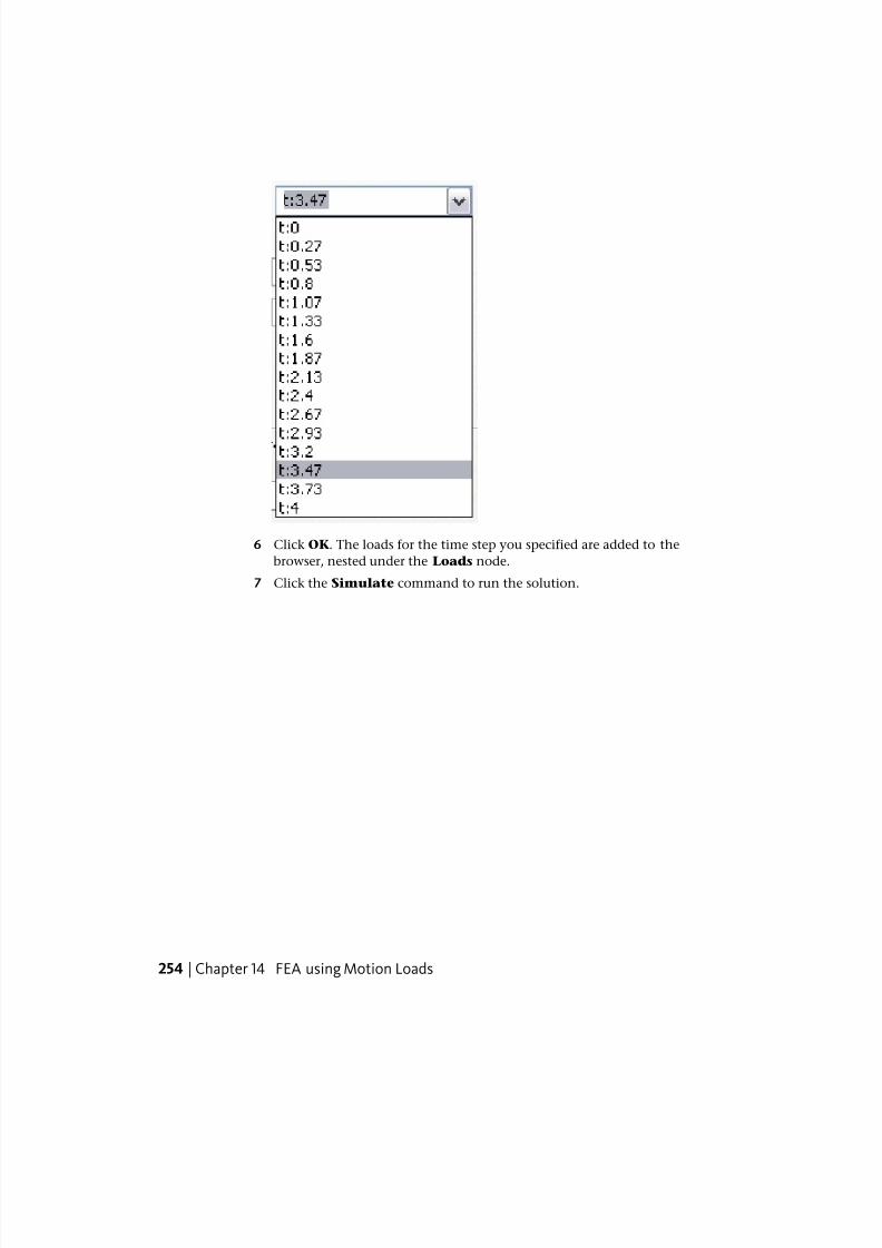
8/20/2019 Stress Analysis INVENTOR
http://slidepdf.com/reader/full/stress-analysis-inventor 260/266
6 Click OK. The loads for the time step you specified are added to the
browser, nested under the Loads node.
7 Click the Simulate command to run the solution.
254 | Chapter 14 FEA using Motion Loads

8/20/2019 Stress Analysis INVENTOR
http://slidepdf.com/reader/full/stress-analysis-inventor 261/266
8 When the simulation finishes, evaluate the results for that motion
interval.
Previous (page 249) | Next (page 256)
Use the Motion Loads in Stress Analysis | 255

8/20/2019 Stress Analysis INVENTOR
http://slidepdf.com/reader/full/stress-analysis-inventor 262/266
Generate a report
Finally, you can generate a report of the analysis results. The report pertains
to the selected time step at the time the report is generated.
1 In the Report panel, click Report.
2 In the Report dialog box, specify the information you want included in
the report.
■ If you want a complete report, click OK and the report will proceed.
■ If you want only certain information in the report, click Custom
and then specify the content for the report.
The report displays in your internet browser or as a Word document,depending on the output format you select. The report and associated
files are saved to the location designated in the Report dialog box. By
default, this location is the same as the part or assembly you are
analyzing.
If you want to save multiple reports, do one of the following
■ Use Save As in your internet browser to save a copy of each report.
■ Rename the report file and generate an additional report. Repeat as
appropriate.
Previous (page 253) | Next (page 257)
256 | Chapter 14 FEA using Motion Loads

8/20/2019 Stress Analysis INVENTOR
http://slidepdf.com/reader/full/stress-analysis-inventor 263/266
Summary
In this tutorial, you learned how to:
■ Generate motion loads for a selected part.
■ Access and use those loads within Stress Analysis.
■ Generate reports of analysis results.
Remember to check Help for further information.
Previous (page 256)
Summary | 257

8/20/2019 Stress Analysis INVENTOR
http://slidepdf.com/reader/full/stress-analysis-inventor 264/266
258

8/20/2019 Stress Analysis INVENTOR
http://slidepdf.com/reader/full/stress-analysis-inventor 265/266
Index
C
coherent masses and inertia 207continuity of laws 207
D
dynamic simulationassumptions 207coherent masses and inertia 207continuity of laws 207
relative parameters 207results 207
O
Output Grapher 208, 217
R
relative parameters 207
259 | Index

8/20/2019 Stress Analysis INVENTOR
http://slidepdf.com/reader/full/stress-analysis-inventor 266/266


![Analysis of lug analysis inventor[1] - Autodesk · 2009-04-23 · Analysis of lug_analysis_inventor[1].ipt Introduction Autodesk Inventor Professional Stress Analysis was used to](https://img.pdfslide.us/doc/110x75/5e92f57d62ff4543182b4ffc/analysis-of-lug-analysis-inventor1-autodesk-2009-04-23-analysis-of-luganalysisinventor1ipt.jpg)


![Autodesk Inventor Pro 9 Stress Analysis[1]. Getting Started](https://img.pdfslide.us/doc/110x75/577d34471a28ab3a6b8d6f05/autodesk-inventor-pro-9-stress-analysis1-getting-started.jpg)