1 | P a g e

Strategies for Achieving Optimal Gasoline Blending

By: David S. Seiver (Valero) & Brian Stefurak (Honeywell)

ABSTRACT

Solomon issued a report on Gasoline and Diesel Quality Analysis in 2010 that showed that the

“monetized difference in gasoline property give-away between the average refiner worldwide

and the top 25% is estimated to be more the $0.55/bbl.” This translates into millions of dollars

of clean product blending optimization opportunity for the average refinery.

Several strategies exist around control method, certification method, waiver methodology,

blend flexibility, blend frequency, and analytical equipment used, not to mention specific

techniques within these strategies that can be used to move your refinery closer to optimal

gasoline blending. These strategies and some techniques and the rationale behind each of

them will be examined.

BIOGRAPHIES

Dave S. Seiver, P.E. has over 20 years experience in the Petrochemical & Industrial Gas

industries. Dave currently is the Manager of Blending APC Technology for Valero. Prior to

coming to Valero, Dave spent four years specialized in Gasoline & Diesel Blend Optimization for

ConocoPhillips at their Wood River Refinery as well as providing technical project assistance to

some of their other sites. Dave has extensive expertise in APC, Blending Optimization, NIR

modeling, and has two U.S. patents in the APC field and one patent-pending for RBOB Gasoline

Optimization using Chemometric Methods. Dave is a registered professional engineer in the

State of Texas.

Brian Stefurak, P.E. has over 20 years experience in Process Automation. Brian currently is the

Blending and Movement Automation Business Consultant for Honeywell’s Advanced Solutions.

In Brian’s years with Honeywell, he has been involved in all aspects of Honeywell’s offsites

automation solutions, from project to support to development to consulting. Brian has been

involved in over a dozen major offsite automation projects and has a perspective on blending

from on-site discussions with more than 50 refineries. Brian is a registered professional

engineer in the Province of Ontario.

2 | P a g e

In June 2010, Solomon & Associates issued a report entitled, “North and South America

Gasoline and Diesel Quality Analysis” outlining a comprehensive look at quality give-away by

refiners for clean products gasoline and diesel. Minimizing the difference between a measured

physical property and a critical specification on a tactical level can have a significant impact on

refinery profitability. According to the report “the monetized difference in gasoline property

give-away between the average refiner worldwide and the top 25% is estimated to be more the

$0.55/bbl, with the difference between the bottom 25% and the best performing 25% being

more than $1.30/bbl.” In a highly competitive, low margin, and currently low refinery

utilization market, this could mean the difference in keeping a refinery running or shutting it

down. Refinery blending typically consists of gasoline and diesel product blending and can be

considered the “cash register” of the refinery. It is the last chance to optimize composition and

to get as close to product specification as possible without excessive giveaway. If there is

specification give-away at blending, it is truly lost revenue and cancels out benefits gained in

upstream unit process areas. At a typical refinery, optimized blending could represent more

than 50% of the total Advanced Process Control (APC) savings, and may exceed $20 million/year

in bottom-line savings. Bear in mind that a small reduction in give-away yields impressive

results through scale-up.

As shown in Figure 1, there are five (5) basic elements of refinery blending complexity that

defines a refinery’s overall product blending strategy. They are Blend Frequency, Blend

Flexibility, Waiver Methodology, Certification Method, and Control Method.

In practice, there are several permutations that span the continuum from optimal to

undesirable. A pragmatic starting point for optimization of refinery blending would begin by

locating a profile matching your refinery’s operations in the table. Throughout this discussion,

we will work from the optimal (green in Figure 1) starting profile, stepping backwards towards

the least preferred profile, thereby illustrating some cost or benefit impacts associated with

each profile bifurcation. The intention is for blending and APC engineers to identify where they

are in their current product blending strategy, and then determine the next logical step(s) to a

more optimal blending strategy. The examples in this article will hopefully help when justifying

a move in that direction. It is not necessary to implement all of the steps from the current to

the optimum, but rather the step(s) most cost effective to the local situation.

3 | P a g e

Figure 1 Refinery blending complexity / optimization matrix

Cost of Blend Frequency

As a general rule, shorter-in-time (smaller-in-volume) blends generally allow for more

commercial opportunities than longer blends (think premiums). However, pragmatic

limitations exist, such as minimum time to get the blend on-spec, equipment stabilized and spot

samples taken and analyzed. Less than eight hours is generally regarded as risky considering the

criteria mentioned earlier. However, this usually would facilitate blends as small as 20 000 bbls

(at rates of 2500 bbls/hr), which could lead to more niche or spot commercial sales

opportunities than those refineries restricted to, say, 100 000 bbls minimum blends. The main

challenge to being able to make smaller blends is ensuring a quality system around the blending

controls/systems that will enable you to minimize specification.

Control method Certification method Waiver methodology Blend flexibility Blend frequency Benefit impact

Short duration blends

(small batches)Optimal

Long duration blends (large

batches) only

Commercial "small sales"

opportunities penalty

Short duration blends

Long duration blends only

Short duration blends

Long duration blends only

Short duration blends

Tank blending Long duration blends only

Short duration blends

Long duration blends only

Short duration blends

Long duration blends only Least desirable

Same as above + limits markets /

customers one can sell product to

Same as above + must account for

primary method reproducibility =>

automatic giveaway

Throughput penalty associated

with blend "fix-ups" & more on-

site tankage

*Same as above + more spot

samples needed meaning more

lab analysis / personnel & limits

minimum blend duration

In-line blending

Many grades and/or

recipe types

Few grades and/or

recipe types

Many grades and/or

recipe types

Few grades and/or

recipe types

*Off-line Off-line

In-line blending

Tank blending

Many grades and/or

recipe types

On-lineIn-line blending

(direct to pipeline)

Few grades and/or

recipe types

On-line

Off-line

4 | P a g e

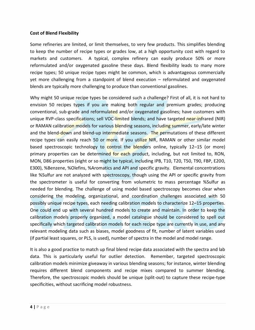
Cost of Blend Flexibility

Some refineries are limited, or limit themselves, to very few products. This simplifies blending

to keep the number of recipe types or grades low, at a high opportunity cost with regard to

markets and customers. A typical, complex refinery can easily produce 50% or more

reformulated and/or oxygenated gasoline these days. Blend flexibility leads to many more

recipe types; 50 unique recipe types might be common, which is advantageous commercially

yet more challenging from a standpoint of blend execution – reformulated and oxygenated

blends are typically more challenging to produce than conventional gasolines.

Why might 50 unique recipe types be considered such a challenge? First of all, it is not hard to

envision 50 recipes types if you are making both regular and premium grades; producing

conventional, sub-grade and reformulated and/or oxygenated gasolines; have customers with

unique RVP-class specifications; sell VOC-limited blends; and have targeted near-infrared (NIR)

or RAMAN calibration models for various blending seasons, including summer, early/late winter

and the blend-down and blend-up intermediate seasons. The permutations of these different

recipe types can easily reach 50 or more. If you utilize NIR, RAMAN or other similar model

based spectroscopic technology to control the blenders online, typically 12–15 (or more)

primary properties can be determined for each product, including, but not limited to, RON,

MON, D86 properties (eight or so might be typical, including IPB, T10, T20, T50, T90, FBP, E200,

E300), %Benzene, %Olefins, %Aromatics and API and specific gravity. Elemental concentrations

like %Sulfur are not analyzed with spectroscopy, though using the API or specific gravity from

the spectrometer is useful for converting from volumetric to mass percentage %Sulfur as

needed for blending. The challenge of using model based spectroscopy becomes clear when

considering the modeling, organizational, and coordination challenges associated with 50

possibly unique recipe types, each needing calibration models to characterize 12–15 properties.

One could end up with several hundred models to create and maintain. In order to keep the

calibration models properly organized, a model catalogue should be considered to spell out

specifically which targeted calibration models for each recipe type are currently in use, and any

relevant modeling data such as biases, model goodness of fit, number of latent variables used

(if partial least squares, or PLS, is used), number of spectra in the model and model range.

It is also a good practice to match up final blend recipe data associated with the spectra and lab

data. This is particularly useful for outlier detection. Remember, targeted spectroscopic

calibration models minimize giveaway in various blending seasons; for instance, winter blending

requires different blend components and recipe mixes compared to summer blending.

Therefore, the spectroscopic models should be unique (split-out) to capture these recipe-type

specificities, without sacrificing model robustness.

5 | P a g e

Figure 2 Spectroscopic Analyzer Model Catalog

Currently there is an ASTM industry sub-team working on a Standard Test Method for Infrared

Determination of Properties of Spark-Ignition Engine Fuels Using Direct Match Comparison

Technique.

Another way to maximize blend flexibility would be to increase the number of blend

components, in essence increasing the degrees of freedom the optimizer has at its disposal. If

there is a way to segregate a mixed or multi-component stream further into different blend

components, say with similar octane values but drastically different RVP values, this will be

advantageous in optimizing product blending. So, for example, if your refinery has some mixed

or multi-component streams with low octane and high RVP, you might consider re-routing one

of the streams that might be similarly low octane but low RVP as a separate component that

could be utilized in summer reformulated blending, where the octane specification is often

easier to achieve than RVP. This is a common optimization strategy used with mixed-cat

naphtha streams where the heavy naphtha stream is segregated from the lighter stream(s).

6 | P a g e

Cost of Waiver Methodology

There are two general methodologies associated with where refiners blend their products: in-

line or pipeline blending, and tank blending.

Typically, in-line blending requires a regulatory

blend waiver that specifies the refiner’s systems

to produce on-spec products directly into a

pipeline. The obvious risk/reward proposition

with in-line blending is the lack of “buffer to fix-

up” blends that tank blending allows, with the

obvious benefit of less tankage and higher

refinery product throughput. The effect on

throughput can be illustrated in the following

example to the right:

The outcome with finished product tank

blending is 15% additional time to move the

same barrels of product, or a reduction in

throughput of 15%.

Further impacting this imbalance is the systemic giveaway inherent to tank (batch) blending. In

the above example, it is assumed that the two cases yield exactly the same final result in

product quality and reduced giveaway. In fact, Case 2 almost always involves expected

giveaway in the “fix-up” or correction blend because of the need to be on-spec in just one

iteration. The same throughput restrictions prevent a blending scenario where after an 90 000

bbl initial blend where the first correction blend is 5000 bbl, another set of testing and analysis

is done, a second correction blend of 3000 bbl is done, another set of testing and analysis is

done, a third correction blend of 1000 bbl is done, and so on. The repeated and hopefully

smaller correction blends are done until the tank is ‘just right’. Since no actual refiner can wait

on repeated correction blends, the first correction blend targets a giveaway on critical

properties to ensure the blend is on-spec or better after only one correction. By comparison,

Case 1 with online analysis and recipe adjustment performs correction blends with each cycle

of the blend optimizer and accurately measuring actual blend results long prior to blend

completion. In a sense, the inline example is allowed to continuously play with the blend until

it is ‘just right’, often long before the end of the blend volume.

7 | P a g e

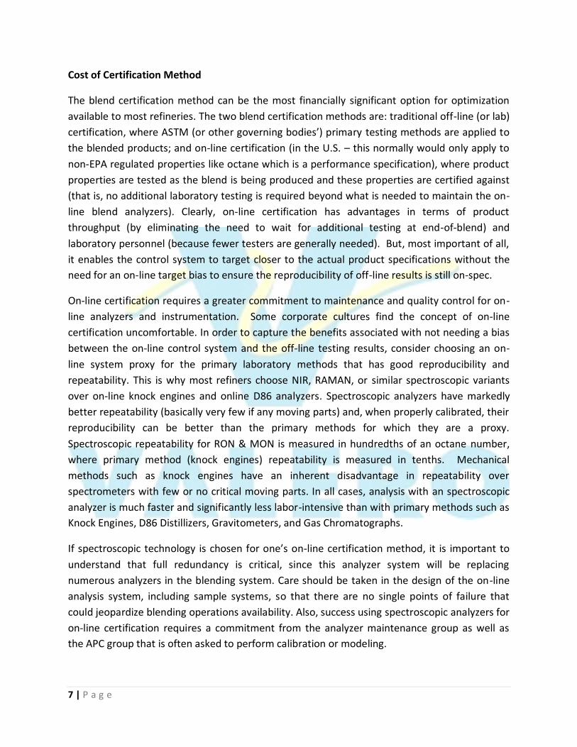
Cost of Certification Method

The blend certification method can be the most financially significant option for optimization

available to most refineries. The two blend certification methods are: traditional off-line (or lab)

certification, where ASTM (or other governing bodies’) primary testing methods are applied to

the blended products; and on-line certification (in the U.S. – this normally would only apply to

non-EPA regulated properties like octane which is a performance specification), where product

properties are tested as the blend is being produced and these properties are certified against

(that is, no additional laboratory testing is required beyond what is needed to maintain the on-

line blend analyzers). Clearly, on-line certification has advantages in terms of product

throughput (by eliminating the need to wait for additional testing at end-of-blend) and

laboratory personnel (because fewer testers are generally needed). But, most important of all,

it enables the control system to target closer to the actual product specifications without the

need for an on-line target bias to ensure the reproducibility of off-line results is still on-spec.

On-line certification requires a greater commitment to maintenance and quality control for on-

line analyzers and instrumentation. Some corporate cultures find the concept of on-line

certification uncomfortable. In order to capture the benefits associated with not needing a bias

between the on-line control system and the off-line testing results, consider choosing an on-

line system proxy for the primary laboratory methods that has good reproducibility and

repeatability. This is why most refiners choose NIR, RAMAN, or similar spectroscopic variants

over on-line knock engines and online D86 analyzers. Spectroscopic analyzers have markedly

better repeatability (basically very few if any moving parts) and, when properly calibrated, their

reproducibility can be better than the primary methods for which they are a proxy.

Spectroscopic repeatability for RON & MON is measured in hundredths of an octane number,

where primary method (knock engines) repeatability is measured in tenths. Mechanical

methods such as knock engines have an inherent disadvantage in repeatability over

spectrometers with few or no critical moving parts. In all cases, analysis with an spectroscopic

analyzer is much faster and significantly less labor-intensive than with primary methods such as

Knock Engines, D86 Distillizers, Gravitometers, and Gas Chromatographs.

If spectroscopic technology is chosen for one’s on-line certification method, it is important to

understand that full redundancy is critical, since this analyzer system will be replacing

numerous analyzers in the blending system. Care should be taken in the design of the on-line

analysis system, including sample systems, so that there are no single points of failure that

could jeopardize blending operations availability. Also, success using spectroscopic analyzers for

on-line certification requires a commitment from the analyzer maintenance group as well as

the APC group that is often asked to perform calibration or modeling.

8 | P a g e

On-line certification requires a more focused approach to analyzer diagnostics. Fortunately,

most spectroscopic analyzers come equipped with powerful, and often ignored or under-

utilized, on-line diagnostic capabilities that should be exploited to ensure a robust on-line

certification system. On-Line blending feedback based on the status of the spectroscopic

analyzer’s real-time diagnostics for each inferred property such as the Residual Ratio (RR)

and/or the Mahalanobis Distance (M-Dist) should be built into the blending control system, and

appropriate standard operating procedures (SOPs) developed so that blending operators know

how to react (i.e. take additional spot samples within the blend) when the on-line analyzers are

telling them that the confidence of the inferred property(s) is questionable (i.e. high RR and/or

M-Dist values). Long-term historical trends of these valuable on-line diagnostic tools should be

analyzed in the routine QC meetings that are part of a robust on-line certification system. A

typical spectroscopic analyzer analysis display is shown below in Figure 3. Examples of

performance data are contained in the display. The left quadrant property data includes both

red highlighting for off-spec results and red and orange underlining of results to indicate

questionable quality of results as determined by the analyzer itself (spectral inconsistencies

between measured and modeled, etc.). Data to the bottom and right of the display shows

overall performance and fault information for the analyzer based on flows or physical faults.

Where the off-spec results are commonly used to correct a given blend, the parallel analyzer

performance numbers should be used to correct the model and analyzer dynamics.

Figure 3 Spectroscopic Analyzer Diagnostics Control System Graphic

9 | P a g e

Cost of Control Method

In common with certification methodology, control methodology for refinery blending also falls

into one of two general classifications: on-line or off-line. As on-line control is the de facto

standard in refining, it is the only methodology to be discussed here. The control method is the

mechanism by which the tender is created. This mechanism includes the process control

hardware and software, and the interface with the refinery planning cycle.

The control method has a choice of objectives. Most on-line Single-Blend Optimizers, or SBO,

have several optimization objective functions to choose from, including minimum cost,

minimum giveaway or minimum blend recipe deviation. Minimum blend recipe deviation

should ideally be a refinery’s optimum strategy if the multi-period recipe planning is extremely

accurate and optimum over the entire multi-period plan. In practice, this is rarely, if ever, the

case, or correct for a fleeting period of time and thus unrealizable, due to commercial or

logistical reasons or refinery dynamics. Changing unit conditions, tank layering of components,

and the age of component property data all combine to create different initial blend conditions

to those expected in the plan. Generally the APC engineer is left to choose between the

minimum cost and minimum give-away objective functions.

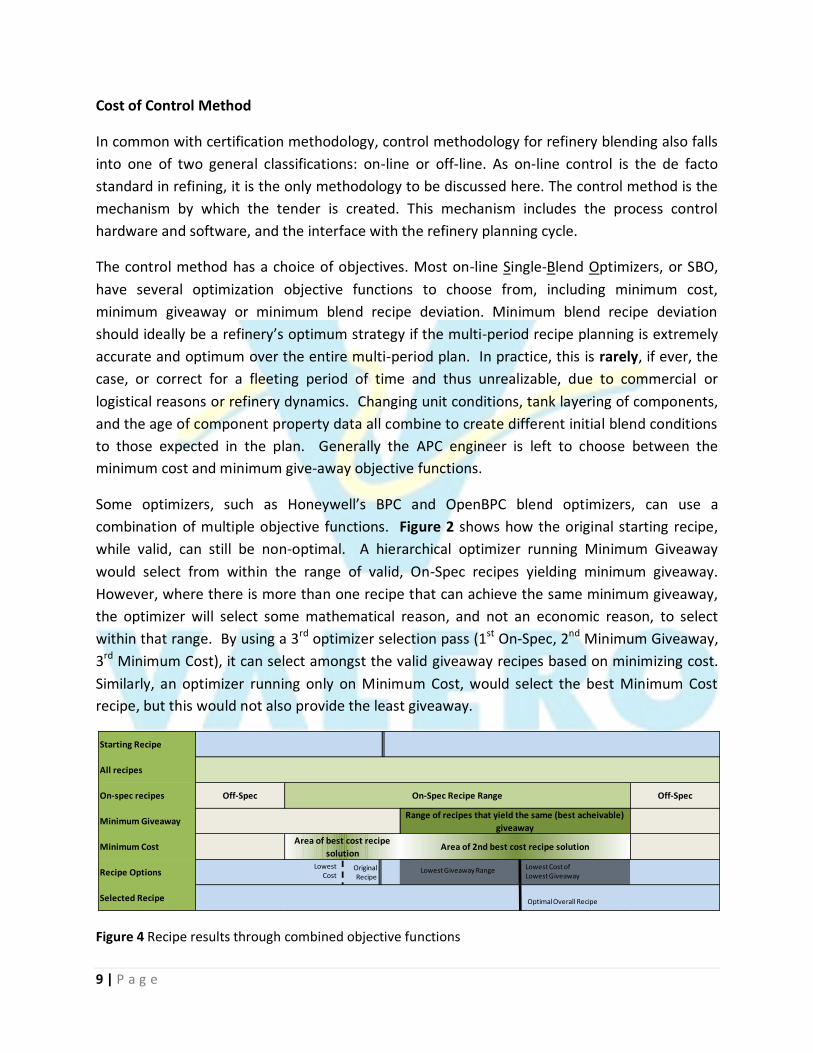
Some optimizers, such as Honeywell’s BPC and OpenBPC blend optimizers, can use a

combination of multiple objective functions. Figure 2 shows how the original starting recipe,

while valid, can still be non-optimal. A hierarchical optimizer running Minimum Giveaway

would select from within the range of valid, On-Spec recipes yielding minimum giveaway.

However, where there is more than one recipe that can achieve the same minimum giveaway,

the optimizer will select some mathematical reason, and not an economic reason, to select

within that range. By using a 3rd optimizer selection pass (1st On-Spec, 2nd Minimum Giveaway,

3rd Minimum Cost), it can select amongst the valid giveaway recipes based on minimizing cost.

Similarly, an optimizer running only on Minimum Cost, would select the best Minimum Cost

recipe, but this would not also provide the least giveaway.

Figure 4 Recipe results through combined objective functions

Starting Recipe

All recipes

On-spec recipes Off-Spec Off-Spec

Minimum Giveaway

Minimum CostArea of best cost recipe

solution

Recipe Options

Selected Recipe

Range of recipes that yield the same (best acheivable)

giveaway

On-Spec Recipe Range

Area of 2nd best cost recipe solution

Lowest Cost

Lowest Cost ofLowest Giveaway

Lowest Giveaway RangeOriginal Recipe

Optimal Overall Recipe

10 | P a g e

However, deviation of the recipe from plan should be tracked and minimized where possible.

Ideally, the multi-period planning software should download suitable min/max recipe

percentages that the single-blend optimizer should stay within, so as not to force the multi-

period plan infeasible.

While the optimizations methods of minimum cost and minimum give-away appear very similar

at first sight, there are subtle differences in their operation and in the results they produce.

Minimum cost tries to create an on-spec blend using the least costly combination of blend

components (i.e. cheapest blend), which does not ensure minimum specification giveaway,

whereas minimum give-away tries to minimize specification giveaway without regard for

utilizing the least costly blend components (though most modern SBO incorporate multi-level

optimization which can combine the benefits of both strategies to some extent). An important

distinction between the two strategies is that minimum giveaway is based on real costs that are

outside the refinery’s economic envelope, whereas minimum cost is based on internal shadow

pricing of components that are not always correlated with actual costs. Therefore, it is

generally advisable to set the primary optimization strategy to minimum giveaway, with a

secondary optimization strategy of minimum cost, and most contemporary single-blend

optimizers can be set up this way. Additionally, in the most common scenario, minimum

giveaway captures some idea of cost, if only because the highest specification components are

often either the most expensive or in the shortest supply.

Another important facet to optimal on-line blend control is the reliability of the blend recipe

data, both initial recipe and blend values, which are obtained from the off-line blend recipe

planning software, or Multi-Period Blend Optimizer (MPBO). Experience has shown that

significant deviation from MPBO initial blend recipes often leads to sub-optimal final product

blends (i.e. giveaway) and risks inventory control issues. This is especially true for blending

systems that are designed to allow “barrel splitting” among product tenders (i.e. blend segment

control is one common strategy), where poor quality initial recipes will lead to large deviations

in product specifications early in the blend, which can never be recovered.

Often, the off-line blend recipe generation tool determines the blend values (roughly, the

steady-state gains used by the optimizer if nonlinear blend equations are not used in the on-

line optimizer) for each blend, and the accuracy of these blend values is important for good

blend control. This is fairly obvious from a multivariable control perspective, where APC

engineers are familiar with optimizer cycling associated with incorrect steady-state gains.

11 | P a g e

Table 1

If your refinery makes oxygenated gasoline, both the off-line blend recipe generation tool and

the online blend optimizer should take into account the non-linear blending effect (aka

“ethanol boost”) that oxygenate induces in blend properties. Some oxygenates like ethanol (the

most common in the U.S.) are not allowed in product pipelines because of corrosion problems

(ethanol is hydrophilic); they are therefore typically added at product terminals. As a

consequence, refineries typically blend neat reformulated/oxygenated gasoline (RBOB), and

Conventional oxygenated gasoline (CBOB), sans ethanol. It is also well known that the so-called

ethanol boost effect on the final blended gasoline’s properties is both recipe-dependent and

non-linear. The ratio of olefins to aromatics used in the neat blendstock significantly

determines the final blended octane of oxygenated gasolines. An example of this is illustrated

in Table 1.

This boost effect should be properly modeled to optimize RBOB/CBOB gasoline blends, and

properly accounted for in both the off-line and on-line blending systems. Estimating the

ethanol boost a priori as opposed to directly measuring “blended properties” throughout the

blend will ultimately lead to either excessive give-away (i.e. you must target worse case low

boost effect which will lead to give-away if the olefins/aromatics ratio deviates substantially

throughout the blend), or in limited blend optimization flexibility (i.e. if you clamp down the

olefins/aromatics ratio you might risk give-away or sub-optimal blends – more expensive

blends). With oxygenated blends becoming more prevalent, this is an area ripe for

optimization.

The ability to examine this effect by refiner is helped by the amount of raw data available. Each

and every blend contains the information on how that particular recipe mix (based on final

component volumes for the blend) behaved in generating the final property specifications.

Regular KPI analysis of actual blend yields to initial starting recipes will show the accuracy of the

current planning and modeling techniques.

RecipeNeat

octane

Blended

octane

EtOH octane

boost

High aromatics; low olefins blend 91.6 93.2 1.6Low aromatics; high olefins blend 91.6 94.9 3.3

RBOB Recipe dependency of ethanol boost effect on octane

12 | P a g e

Conclusions

Some basic elements of refinery blending complexity have been described in sufficient detail to

enable blending and APC engineers to plan the next step(s) towards optimal refinery blending

at their location. Furthermore, specific examples of implementable measures, techniques and

technologies have been described, with some economic considerations presented where

applicable.

Not all refineries will be able to get to the ideal refinery blending profile, but instead may only

move incrementally towards that objective. It is the refinery’s challenge to identify its unique

place in the matrix of refinery blending complexity and to then to produce a project plan to

reach the next step(s) towards a more optimal state.