Embed Size (px)
Citation preview
EDITED BY XINSHEN DIAO | JAMES THURLOW | SAMUEL BENIN | SHENGGEN FAN
economywide perspectives from country studies
AND PRIORITIESFOR AFRICAN AGRICULTURE
About IFPRI
The International Food Policy Research Institute (IFPRI®) was established in 1975 to identify and analyze alternative national and international strategies and policies for meeting food needs of the developing world on a sustainable basis, with particu-lar emphasis on low-income countries and on the poorer groups in those countries. While the research effort is geared to the precise objective of contributing to the reduction of hunger and malnutrition, the factors involved are many and wide-ranging, requiring analysis of underlying processes and extending beyond a narrowly defi ned food sector. The Institute’s research program refl ects worldwide collabora-tion with governments and private and public institutions interested in increasing food production and improving the equity of its distribution. Research results are disseminated to policymakers, opinion formers, administrators, policy analysts, researchers, and others concerned with national and international food and agricul-tural policy.
IFPRI is a member of the CGIAR Consortium.


Strategies and Priorities for African Agriculture
Economywide Perspectives from Country Studies

Strategies and Priorities for African Agriculture
Economywide Perspectives from Country Studies
Edited by Xinshen Diao, James Thurlow, Samuel Benin, and Shenggen Fan
International Food Policy Research InstituteWashington, D.C.
Copyright © 2012 International Food Policy Research Institute. All rights reserved. Contact [email protected] for permission to republish.
International Food Policy Research Institute2033 K Street, NWWashington, DC 20006-1002, USATelephone +1-202-862-5600www.ifpri.org
DOI: http://dx.doi.org/10.2499/9780896291959
Library of Congress Cataloging-in-Publication Data
Strategies and priorities for African agriculture : economywide perspectives from country studies / edited by Xinshen Diao . . . [et al.]. p. cm. Includes bibliographical references and index. ISBN 978-0-89629-195-9 (alk. paper) 1. Agriculture—Economic aspects—Africa. 2. Agriculture— Economic aspects—Africa—Case studies. 3. Rural development—Africa. 4. Poverty—Africa. 5. Agriculture and state—Africa. I. Diao, Xinshen.HD2117.S75 2012338.1096—dc23 2011043673
Contents
Preface ix
Acknowledgments xi
Chapter 1 African Agriculture and Development 1 Joanna Brzeska, Xinshen Diao, Shenggen Fan,
and James Thurlow
Chapter 2 A Recursive Dynamic Computable General Equilibrium Model 17
Xinshen Diao and James Thurlow
Chapter 3 Estimating Public Agricultural Expenditure Requirements 51
Samuel Benin, Shenggen Fan, and Michael Johnson
Chapter 4 Kenya 71 James Thurlow, Jane Kiringai, and Madhur Gautam
Chapter 5 Ethiopia 107 Xinshen Diao, Alemayehu Seyoum Taffesse, Paul Dorosh,
James Thurlow, Alejandro Nin Pratt, and Bingxin Yu
Chapter 6 Ghana 141 Clemens Breisinger, Xinshen Diao, James Thurlow,
Samuel Benin, and Shashidhara Kolavalli
Chapter 7 Rwanda 165 Xinshen Diao, Shenggen Fan, Sam Kanyarukiga,
and Bingxin Yu
viii CONTENTS
Chapter 8 Nigeria 211 Xinshen Diao, Manson Nwafor, Vida Alpuerto,
Kamiljon T. Akramov, Valerie Rhoe, and Sheu Salau
Chapter 9 Malawi 245 Samuel Benin, James Thurlow, Xinshen Diao,
Christen McCool, and Franklin Simtowe
Chapter 10 Uganda 281 Samuel Benin, James Thurlow, Xinshen Diao,
Allen Kebba, and Nelson Ofwono
Chapter 11 Zambia 317 James Thurlow, Samuel Benin, Xinshen Diao,
Henrietta Kalinda, and Thomson Kalinda
Chapter 12 Mozambique 349 James Thurlow
Chapter 13 Tanzania 371 Karl Pauw and James Thurlow
Chapter 14 Lessons Learned and Remaining Challenges 399 Xinshen Diao and James Thurlow
Contributors 415
Index 419
Preface
For the first time in many years, Africa has enjoyed a period of strong and sus-tained economic growth. The agricultural sector has also grown at a moderate rate, and this growth has contributed to significant reductions in poverty in
many African countries. This improved agricultural performance is consistent with continentwide initiatives—one of the most important being the Comprehensive Africa Agriculture Development Programme—which aim to raise rural incomes, reduce poverty, and increase food and nutrition security through agricultural invest-ment and growth.
This book examines the potential of agriculture to contribute to national growth and poverty reduction. It also evaluates the fi nancial costs of accelerating agricultural growth. The analysis is based on ten country case studies that apply similar economywide approaches to linking growth, poverty, and investment. The fi ndings indicate that, in most African countries, improving agriculture’s performance is essential to achieving pro-poor growth. They also point to export agriculture having high growth potential and becoming a prominent part of agri-cultural strategies. The research shows that broad-based growth will be diffi cult to achieve without expanding staple-foodcrop production and livestock produc-tion, since only they have the scale and linkages to poor households needed to reduce national poverty within a reasonable period of time. Finally, the case stud-ies confi rm the need for greater investment in agriculture. However, the effi ciency of agricultural investments will have to improve if development targets are to remain attainable.
This book provides a structured approach to evaluating agricultural develop-ment strategies at the country level. The case studies demonstrate the application of important analytical methods that can be adopted by governments and researchers

x PREFACE
in developing countries. Of course, not all challenges facing agricultural develop-ment can be addressed by the methods presented in this volume. For example, analysis of the political economy of investment decisionmaking is also important to promot-ing agricultural growth. Nevertheless, this book provides valuable practical insights and guidance and will contribute to strategic thinking and investment planning and implementation in many African countries.
Acknowledgments
Several people have made this book possible. We are grateful to Peter Hazell, who initiated the evidence-based debates on the role of agriculture in the early 2000s that led to the development and application of computable
general equilibrium models for agricultural growth–poverty analysis in an economy-wide framework. Jeff Hill encouraged this approach but also challenged the IFPRI research team on how to use it to address agricultural strategic development issues. The Comprehensive Africa Agriculture Development Programme (CAADP) pro-vided the context for applying this economywide analytical framework in the countries studied. While doing our research, we interacted with and learned from so many individuals, organizations, and agencies that it would be impossible to attempt to list all of them without leaving some out.
We thank Ousmane Badiane for his leadership of the IFPRI-CAADP agree-ment, through which part of the funding for this work was made available. Financial support was also provided by the Belgian Trust Funds, the Bill & Melinda Gates Foundation, the Canadian International Development Agency, the European Com-mission, the Swedish International Development Cooperation Agency, the U.K. Department for International Development, the U.S. Agency for International Development, and the World Bank.

C h a p t e r 1
African Agriculture and DevelopmentJoanna Brzeska, Xinshen Diao,
Shenggen Fan, and James Thurlow
A fter decades of income divergence between Africa and the rest of the world, a new era appears to have begun in many African countries.1 The decade since 2000 has been one of macroeconomic stability, sustained economic
growth, and improved governance. Although this performance was disrupted by the global recession and food crises in 2008–10, Africa was one of the less affected of the world’s developing regions. In fact, not only did growth accelerate in Africa during the 2000s, but this was also the first decade since the 1970s when Africa was not the slowest growing developing region (World Bank 2010a).2 It therefore marks a historic break from decades of internal and external deficits, economic stagna-tion, and political turmoil. Moreover, a wide range of African countries performed well, including oil-exporting and resource-rich countries, large and middle-income countries, and coastal and low-income countries (Arbache et al. 2008). The new millennium has heralded Africa’s first “decade of growth.”
What is not clear, however, is whether Africa’s stronger and sustained growth will successfully lay the foundations for longer term economic transformation and prosperity. Despite some positive trends, many problems and challenges still remain. High levels of poverty, poor health, and malnutrition continue to plague many African countries. As a developing region, Africa still experienced an increase in its number of poor people during 2000–05 (World Bank 2010a). Moreover, some of Africa’s fastest growing economies have not signifi cantly reduced poverty, such as Mozambique and Tanzania (Republic of Mozambique 2010; United Republic of Tanzania 2010). These disappointing social outcomes are due to weak institutional, policymaking, and research capacity and to insuffi cient public investments that are
2 JOANNA BRZESKA ET AL.
often misallocated and ineffi cient (see Fan 2008). The important role of evidence-based research in formulating pro-poor development strategies means that the lack of research capacity and inadequate human resources have also been a major hurdle to development.
Most of Africa’s poor population is to some degree dependent on farming. Therefore, fostering agricultural growth is often seen as being central to develop-ment strategies aimed at reducing poverty and hunger in the region (Thirtle, Lin, and Piesse 2003). Not only is poverty still concentrated in rural areas, but the agri-cultural sector also typically accounts for a large share of national income and employment. However, despite its importance, agricultural growth in Africa still lags far behind national overall economic growth, with per capita agricultural incomes expanding at less than 1 percent per year during 2000–09 (World Bank 2010a). This rate was only a third of the nonagricultural sector’s growth rate. From a global perspective, African agriculture has fallen even farther behind that of other developing regions, even during the continent’s more rapid growth period. As a result, the rural–urban divide in Africa has continued to widen.
African heads of state have responded to slow agricultural growth and rural development by adopting the Comprehensive Africa Agriculture Development Programme (CAADP). This is an African-owned initiative to stimulate agriculture on the continent and accelerate agriculture-led growth and poverty reduction under the framework of the New Partnership for Africa’s Development (NEPAD). Among the main principles of the CAADP is the pursuit of a 6 percent annual growth rate in agriculture by allocating at least 10 percent of public resources to the agricultural sector. Although the endorsement of the CAADP represents a strong commitment to agriculture by African governments, its implementation requires analytical sup-port at the country level. For example, analytical support is needed to analyze the role of agriculture and its potential contribution to future development in Africa. What should be the priorities among different subsectors in agriculture? Is 6 percent agricultural growth enough to achieve poverty- and hunger-reduction goals? How many resources are required to support the necessary agricultural growth? How should limited public resources be prioritized?
Debating Agriculture’s Role in African Development African governments have now placed more emphasis on agriculture in their devel-opment strategies than in the past. Yet our understanding of agriculture’s role in countries’ development processes has evolved considerably over the past half century, and the supposed importance of the sector is far from resolved.3 Early “dual-economy” models viewed agriculture as a passive participant, that is, as a tradi-
AFRICAN AGRICULTURE AND DEVELOPMENT 3
tional, low-productivity supplier of food and surplus labor to a modern and more urbanized industrialization process (Adelman 1999). Although raising agricultural productivity was seen as a necessary precondition for development, agriculture itself was not viewed as a major source of national growth and certainly not as a leading sector in a country’s economic transformation. In fact, agriculture’s dependence on fi xed natural resources meant that, in the long run, growth in the sector would be constrained, and its share of the economy would inevitably decline. Agriculture would, however, remain important as a supplier of food. Traditional thinking, therefore, saw agriculture’s role as providing a reserve of low-wage labor and en-suring food security.
The successes of Asia’s Green Revolution caused many people to reassess their understanding of agriculture’s growth potential. New technologies allowed agricul-ture in Asia to raise its productivity, overcome national resource constraints, and transform itself into a modern sector. Underlying agriculture’s contribution to broader development was the sector’s economic linkages to nonagriculture (Johnston and Mellor 1961). Faster agricultural growth was found to stimulate growth in downstream sectors and, by raising real incomes, generate demand for both farm and nonfarm goods. Agriculture’s linkages were also shown to be particularly impor-tant for rural development (see, for example, Haggblade, Hazell, and Brown 1989; Haggblade, Hammer, and Hazell 1991). More recent evidence goes beyond linkages to emphasize the benefi ts of reducing urban bias in public investments and improv-ing nutrition (Timmer 2002). Together, these insights from Asia led many to assign agriculture a more prominent or active role in the development process—one that might be transferrable to Africa.
Although the evidence confi rms the central role played by agriculture in Asia, there is still some disagreement over whether the lessons learned two decades ago remain relevant for Africa today. Of course, proponents of agriculture argue that the sector is the largest in Africa, and so without agricultural growth, there is unlikely to be meaningful national growth. Similarly, much of Africa’s nonfarm economy relies on raw agricultural materials, and so African industrialization may also hinge on raising farm production. Moreover, because most of Africa’s poor population still lives in rural areas and depends on agriculture for a livelihood, there is unlikely to be broad-based poverty reduction without at least some acceleration in agricultural growth. Of course, as mentioned above, agriculture has not historically been a major source of economic growth in Africa. However, proponents of African agriculture argue that this is due to long-standing urban bias and underinvestment in the sector (see Fan 2008; Fan and Zhang 2008). Empirical evidence suggests that the returns to agricultural investments are large and rapid agricultural growth is possible, given Africa’s low productivity levels. Proponents therefore see few alternatives to agricul-
4 JOANNA BRZESKA ET AL.
ture in many African countries. They also identify considerable opportunities to accelerate agricultural growth, thereby promoting rural development and reducing poverty.
Not all African development specialists view agriculture in the same positive light. Many remain skeptical about the sector’s ability to play a central role in devel-opment. African agriculture has not been a stellar performer over the long run, and the unfavorable agroecological conditions of many countries mean that the growth experiences of Asia may not be replicable in Africa (see, for example, Collier 2003; Maxwell and Slater 2003). Moreover, the world is now more globalized than it was during the Green Revolution, which may make agriculture-led development more diffi cult to achieve (and possibly make an agricultural foundation for economic transformation unnecessary). For example, it may no longer be necessary for coun-tries to expand domestic food production, as it is now easier to purchase foods from global markets. This may allow African countries to overcome their resource con-straints and poor agroecological conditions, and also to bypass agriculture in their development process (Hart 1998). Those skeptical of agriculture place greater em-phasis on industrialization through mining and manufacturing, or recently, on repli-cating India’s successes in the service sector. From this perspective, nonagriculture, rather than agriculture, should be afforded a more central role in African develop-ment strategies.
Any poverty reduction strategy in Africa must pay some attention to rural incomes, because a large portion of Africa’s poor population lives in these areas. Therefore, the role of agriculture in reducing poverty is perhaps more clear cut, even if one views the sector’s contribution to economic growth as marginal. However, there are sharp differences of opinion over which kind of agricultural growth is most effective at reducing poverty (Dorward et al. 2004). Some practitioners see export crops as having both higher value and a lower dependence on domestic demand and local markets, which are often small and poorly developed in African countries. From this perspective, export-oriented crop production should be afforded the highest priority in agricultural strategies. In contrast, others see a stronger role for smallholder staple foodcrops in raising incomes. Empirical evidence suggests that considerable potential exists for African farmers to trade foodcrops in domestic and regional markets (see Diao and Hazell 2004). From this alternative perspective, an agricultural strategy based on expanding foodcrop production would directly benefi t Africa’s poorest populations. It could also be based on commercialization and trade, rather than on traditional subsistence farming.
There are thus three aspects to the current debate on the role of agriculture in African development. First, it is not clear whether agriculture can generate substan-tial economic growth and poverty reduction in Africa, or whether a development strategy based on industrial growth would be more effective. Answering this ques-
AFRICAN AGRICULTURE AND DEVELOPMENT 5
tion would decide the merits of Africa’s CAADP initiative. Second, in agriculture, it is not certain whether it would be preferable to promote smallholder foodcrops or export-oriented crops. This question is crucial for African governments as they reallocate resources to the agricultural sector under the CAADP. Of course, it should be acknowledged that the debate is really over a matter of emphasis: How much should agriculture or nonagriculture be emphasized in relation to the other? When choices exist, how much public investment should be targeted toward export or foodcrops? Finally, Africa is a large and diverse continent, and so policy prescriptions must refl ect country context—a “one size fi ts all” approach is not possible.
Objective: Identifying Sources of Growth and Poverty Reduction A development strategy would ideally take advantage of all opportunities for growth and poverty reduction. In reality, however, the limited resources of governments imply that sequencing or prioritization of public policies and investments is needed. For many African countries, allocating 10 percent of their budget to agriculture means that fewer resources are available for other interventions or sectors. Thus, although the CAADP strengthens the role of agriculture in development, what is lacking in many African countries is the evidence needed to justify this prioritization and to design agricultural investment plans.
In this book we provide evidence to inform the design the African development strategies and to address the ongoing debate on the role of African agriculture. We develop an economywide modeling framework that captures the linkages between sectoral and national economic growth on the one hand, and spatial and household-level poverty on the other. Within the context of the CAADP, we use this framework to compare different sectoral sources of national and agricultural growth. Our analy-sis is based on 10 country case studies refl ecting the diversity of agroecological conditions and development challenges facing low-income Africa. In most cases we conduct our analysis at both the national and subnational levels, and in all cases we combine economywide modeling with survey-based microsimulation analysis. We also explore a variety of methods to estimate the public resources required to accelerate agricultural growth.
Based on a series of criteria refl ecting the current debate, we use our modeling framework to identify crops and sectors that have the greatest potential to generate pro-poor growth. Individual sectors may have different impacts on national growth and poverty reduction for a variety of reasons. First, certain sectors are already large, and so small improvements in productivity can have large implications for national growth over a reasonable time horizon. Second, smaller sectors may have higher growth potentials, so they can still contribute to overall growth by expanding rap-
6 JOANNA BRZESKA ET AL.
idly. Third, some sectors are more effective at reducing poverty, either because they have stronger linkages to poor households’ income-generation processes, or they produce products that poor households consume intensively. Fourth and similarly, some sectors produce products that are important for households’ nutritional status, especially if essential foods cannot be imported easily. Finally, some sectors may have stronger economywide linkages, such as to downstream processing, and so expand-ing production in these sectors generates more national-level growth. Criteria such as these are determined by a country’s unique structural characteristics and market conditions. Of course, the prioritizations of sectors within a development strategy will ultimately depend on a country’s own development objectives, that is, balancing growth, poverty, and food-security outcomes. Therefore, to inform the debate on African agriculture, it is essential that suitably representative case-study countries are selected.
Country Case Studies
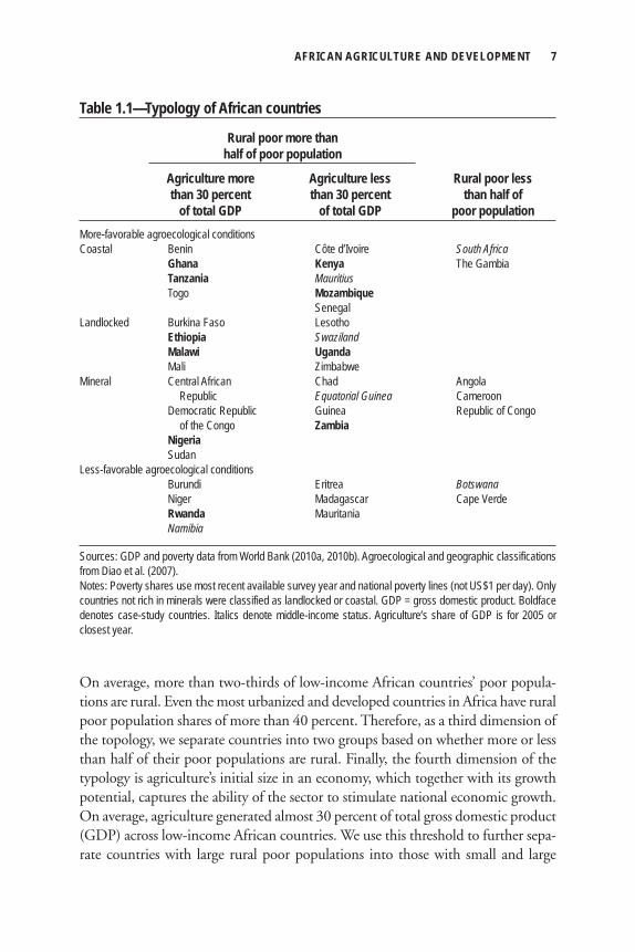
Typology of African CountriesIn selecting our case studies, we fi rst develop a typology of African countries designed to capture four dimensions of the debate on the role of agriculture in development (Table 1.1).4 The fi rst two dimensions relate to natural resource endowments and geographic characteristics. Agriculture’s growth potential depends on agro-ecological conditions. To ensure that we select cases with both high and low agri-cultural potential, we separate countries into those with more- or less-favorable agroecological conditions according to the classifi cation in Diao et al. (2007).5 However, even in countries with favorable conditions, agriculture competes with other sectors for limited resources. Countries with rich mineral and oil endowments may have alternative sources of growth and so are separated in the typology. Furthermore, coastal countries may have advantages in export-oriented agriculture or greater opportunities in nonagricultural sectors. Therefore, coastal and land-locked countries are also separated. The typology identifi es four groups of African countries based on their natural resource endowments and geographic characteris-tics: (1) coastal; (2) landlocked; (3) mineral-rich; and (4) less-favorable agricultural potential. These traits describe the immutable initial conditions in which agriculture and other economic activities must operate.
The other two dimensions of the debate relate to agriculture’s situation in the broader economy and its relationship to poverty reduction. One of the arguments in favor of agriculture playing a central role in development is its strong linkages to poor rural households. To capture this connection, we measure the share of a coun-try’s poor population living in rural areas by using data from World Bank (2010b).
AFRICAN AGRICULTURE AND DEVELOPMENT 7
On average, more than two-thirds of low-income African countries’ poor popula-tions are rural. Even the most urbanized and developed countries in Africa have rural poor population shares of more than 40 percent. Therefore, as a third dimension of the topology, we separate countries into two groups based on whether more or less than half of their poor populations are rural. Finally, the fourth dimension of the typology is agriculture’s initial size in an economy, which together with its growth potential, captures the ability of the sector to stimulate national economic growth. On average, agriculture generated almost 30 percent of total gross domestic product (GDP) across low-income African countries. We use this threshold to further sepa-rate countries with large rural poor populations into those with small and large
Table 1.1—Typology of African countries
Rural poor more than half of poor population
Agriculture more Agriculture less Rural poor less than 30 percent than 30 percent than half of of total GDP of total GDP poor populationMore-favorable agroecological conditionsCoastal Benin Côte d’Ivoire South Africa Ghana Kenya The Gambia Tanzania Mauritius Togo Mozambique Senegal Landlocked Burkina Faso Lesotho Ethiopia Swaziland Malawi Uganda Mali Zimbabwe Mineral Central African Chad Angola Republic Equatorial Guinea Cameroon Democratic Republic Guinea Republic of Congo of the Congo Zambia Nigeria Sudan Less-favorable agroecological conditions Burundi Eritrea Botswana Niger Madagascar Cape Verde Rwanda Mauritania Namibia
Sources: GDP and poverty data from World Bank (2010a, 2010b). Agroecological and geographic classifications from Diao et al. (2007).Notes: Poverty shares use most recent available survey year and national poverty lines (not US$1 per day). Only countries not rich in minerals were classified as landlocked or coastal. GDP = gross domestic product. Boldface denotes case-study countries. Italics denote middle-income status. Agriculture’s share of GDP is for 2005 or closest year.
8 JOANNA BRZESKA ET AL.
agricultural sectors. We therefore have three groups in the typology based on agri-culture’s structural characteristics: (1) countries with a large rural poor population and large agricultural sector, (2) those with a large rural poor population and small agricultural sector, and (3) those with a small rural poor population.
Case Study SelectionWe selected 10 countries from the typology (bolded in the table).6 We exclude middle-income countries from our selection (italicized), as well as countries with less than half of their poor populations in rural areas (that is, the fi nal column of the table). Such countries include Botswana and South Africa, where agriculture has played an important role in past development, but the low agricultural GDP share and rela-tively small rural poor population mean that agriculture is unlikely to be the driver of national growth or poverty reduction in the future.7 Our 10 selected countries cover the continent’s three regions: fi ve from eastern Africa, three from southern Africa, and two from western Africa.
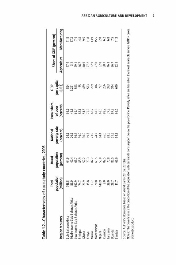
Together the 10 case-study countries accounted for 57 percent of low-income Africa’s total population in 2005 and a similar share of its poor population (Table 1.2). The population of individual countries varies widely, from 141 million in Nigeria to only 9 million in Rwanda. The difference in the per capita GDP is also large, with the highest value four times the size of the lowest value. Nigeria and Zambia have the highest per capita GDPs because of overvalued exchange rates caused by high mineral export prices. The three countries with the lowest income levels are the more agrarian economies of Ethiopia, Malawi, and Rwanda.
Our cases refl ect above- and below-average characteristics for low-income Africa. In six of the countries, agriculture’s share of GDP is above the average for low-income African countries, and in four countries it is below. Moreover, among countries with large agricultural shares, three are greater than 40 percent (Ethiopia, Ghana, and Tanzania), and three are between 30 and 40 percent (Malawi, Nigeria, and Rwanda). We also consider the contribution of manufacturing to GDP: six case studies have above-average shares and four below. Finally, as mentioned above, we exclude from our selection countries with more than half of their poor populations in urban areas. This obviously biases our selection toward countries with larger rural population shares. However, despite this restriction, four of the case studies are more urbanized than the average low-income African country. This balanced selection of countries suggests that our cases are representative of low-income Africa.
Recent Growth and Poverty Reduction Our analysis focuses on the effectiveness of different sources of economic growth in reducing poverty. Although the recent performances of each case study are discussed in detail later in the book, we provide a broad comparison of the 10 countries in
AFRICAN AGRICULTURE AND DEVELOPMENT 9
Tabl
e 1.2—
Char
acte
ristic
s of c
ase-
stud
y cou
ntrie
s, 20
05
To
tal
Rura
l Na
tiona
l Ru
ral s
hare
GD
P
popu
latio
n po
pulat
ion
pove
rty ra
te
of p
oor
per c
apita
Re
gion
/ cou
ntry
(m
illion
) (p
erce
nt)
(per
cent
) (p
erce
nt)
(US$
) Ag
ricul
ture
Ma
nufa
ctur
ing
Sub-
Saha
ran A
frica
748.8
64
.9 54
.2 68
.5 86
4 17
.4 11
.8Mi
ddle-
incom
e Sub
-Sah
aran
Afric
a 56
.0 42
.4 26
.9 45
.3 5,2
21
3.1
17.2
Low-
incom
e Sub
-Sah
aran
Afric
a 69
2.9
66.7
56.4
69.4
513
29.1
7.4Et
hiopia
74
.7 83
.9 39
.0 85
.1 16
5 46
.7 4.8
Ghan
a 21
.9 52
.2 30
.0 51
.5 48
9 40
.9 9.5
Keny
a 35
.8 79
.3 19
.7 79
.0 52
3 27
.2 11
.8Ma
lawi
13.7
82.7
73.9
82.7
209
32.9
13.9
Moza
mbiqu
e 20
.8 65
.5 74
.7 67
.0 31
6 27
.0 15
.5Ni
geria
14
0.9
53.8
64.4
62.5
797
32.8
2.8Rw
anda
9.0
82
.5 76
.6 82
.2 26
6 38
.7 6.2
Tanz
ania
39.0
75.8
88.5
77.3
373
46.1
6.8Ug
anda
28
.7 87
.5 51
.5 87
.3 31
4 26
.7 7.5
Zamb
ia 11
.7 65
.0 64
.3 65
.0 61
0 22
.1 11
.3
Sour
ce: A
uthor
s’ ca
lculat
ions b
ased
on W
orld
Bank
(201
0a, 2
010b
).No
tes: T
he po
verty
rate
is the
prop
ortio
n of th
e pop
ulatio
n with
per c
apita
cons
umpti
on be
low th
e pov
erty
line.
Pove
rty ra
tes ar
e bas
ed on
the l
atest
avail
able
surve
y. GD
P = g
ross
do
mesti
c pro
duct.
Shar
e of G
DP (p
erce
nt)
10 JOANNA BRZESKA ET AL.
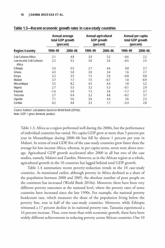
Table 1.3. Africa as a region performed well during the 2000s, but the performance of individual countries has varied. Per capita GDP grew at more than 5 percent per year in Mozambique during 2000–06 but fell by almost 1 percent per year in Malawi. In terms of total GDP, fi ve of the case-study countries grew faster than the average for low-income Africa, whereas, in per capita terms, seven were above aver-age. Agricultural GDP growth accelerated after 2000 in all but two of the case studies, namely, Malawi and Zambia. However, as in the African region as a whole, agricultural growth in the 10 countries has lagged behind total GDP growth.
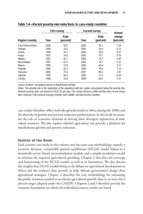
Table 1.4 summarizes recent poverty-reduction trends in the 10 case-study countries. As mentioned earlier, although poverty in Africa declined as a share of the population between 2000 and 2005, the absolute number of poor people on the continent has increased (World Bank 2010a). Moreover, there have been very different poverty outcomes at the national level, where the poverty rates of some countries have increased since the late 1990s. For example, the national poverty headcount rate, which measures the share of the population living below the poverty line, rose in half of the case-study countries. Moreover, while Ethiopia witnessed a 17 percent decline in its national poverty rate, Tanzania experienced a 16 percent increase. Thus, even more than with economic growth, there have been widely different achievements in reducing poverty across African countries. Our 10
Table 1.3—Recent economic growth rates in case-study countries
Annual average Annual agricultural Annual per capita total GDP growth GDP growth total GDP growth (percent) (percent) (percent)
Region / country 1990–99 2000–06 1990–99 2000–06 1990–99 2000–06Sub-Saharan Africa 2.1 4.8 3.0 3.2 –0.6 2.2Low-income Sub-Saharan 2.2 5.3 3.0 3.6 –0.5 2.5 Africa Ethiopia 3.3 5.5 2.7 4.6 0.8 2.7Ghana 4.3 5.0 3.0 3.4 1.6 2.7Kenya 2.2 3.5 1.5 3.0 –0.8 0.8Malawi 3.7 1.7 7.5 –0.7 1.8 –0.9Mozambique 5.5 8.2 4.5 6.4 1.8 5.2Nigeria 2.7 5.5 3.2 5.3 –0.1 2.9Rwanda –1.6 5.0 1.5 3.6 –1.7 2.7Tanzania 2.7 6.4 3.2 4.8 –0.2 3.7Uganda 7.1 5.6 3.6 4.4 3.6 2.3Zambia 0.2 4.8 3.2 1.7 –2.4 2.8
Source: Authors’ calculations based on World Bank (2010a).Note: GDP = gross domestic product.
AFRICAN AGRICULTURE AND DEVELOPMENT 11
case studies therefore refl ect both the general trends in Africa during the 2000s and the diversity of growth and poverty-reduction performances. In this book we exam-ine the role of economic structure in driving these divergent experiences of indi-vidual countries. We also explore whether agriculture can provide a platform for simultaneous growth and poverty reduction.
Outline of the Book Each country case study in this volume uses the same core methodology, namely, a recursive dynamic computable general equilibrium (DCGE) model linked to a household survey–based microsimulation module and a simple simulation model to estimate the required agricultural spending. Chapter 2 describes the coverage and functioning of the DCGE model, as well as its limitations. We also discuss the insights that DCGE models bring to the debate on agricultural development in Africa and the evidence they provide to help African governments design their agricultural strategies. Chapter 3 describes the core methodology for estimating the public resources needed to accelerate agricultural growth (that is, to meet the 6 percent target adopted under the CAADP). Chapters 2 and 3 therefore provide the common foundation on which the individual country studies are based.
Table 1.4—Recent poverty-rate reductions in case-study countries
Annual Rate Rate changeRegion / country Year (percent) Year (percent) (percent)Sub-Saharan Africa 2000 55.0 2005 50.1 –1.54Ethiopia 1999 55.6 2005 39.0 –5.72Ghana 1998 39.1 2006 30.0 –3.27Kenya 1997 19.6 2005 19.7 0.10Malawi 1997 83.1 2004 73.9 –1.66Mozambique 1997 81.3 2003 74.7 –1.41Nigeria 1996 53.9 2003 64.4 2.57Rwanda 1984 63.3 2000 76.6 1.19Tanzania 2000 72.6 2007 88.5 2.87Uganda 1999 60.5 2005 51.5 –2.64Zambia 1998 55.4 2004 64.3 2.51
Source: Authors’ calculations based on World Bank (2010b). Notes: The poverty rate is the proportion of the population with per capita consumption below the poverty line. National poverty rates are based on US$1.25 per day. The survey closest to 2000 and the most recent survey were selected. Sub-Saharan average includes both middle- and low-income countries.
First survey Second survey
12 JOANNA BRZESKA ET AL.
The order of the 10 case studies in Chapters 4–13 is determined by how the core methodology is implemented. More specifi cally, the analysis in each chapter can be separated into two components. The fi rst is the poverty–growth component, which evaluates the linkages between economic growth and poverty in each country. The second is the investment–growth component, which estimates how much public investment is needed to achieve faster growth. The country studies differ in how each component is conducted and how closely tied they are.
In terms of the poverty–growth component, the chapters progress from country studies that adopt a broader view of the debate on the role of agriculture to those with a more detailed focus on the agricultural sector itself. For example, the Kenya and Ethiopia studies (Chapters 4 and 5, respectively) are presented early in the book, because they start by contrasting the effectiveness of aggregate agriculture and nonagriculture on economic growth and employment. They therefore directly address the fi rst area of debate, namely, whether agriculture or nonagriculture should be prioritized in national development strategies. The subsequent case studies focus more on the second aspect of the debate, namely, which agricultural subsectors are most effective at raising growth and reducing poverty. Although every chapter addresses this issue, the later chapters in the book adopt a far more detailed treat-ment of the agricultural sector. For example, the Ghana study (Chapter 6) considers different agroecological zones and how they shape crop and livestock production. The Rwanda study (Chapter 7) and Nigeria study (Chapter 8) also disaggregate agricultural activities geographically—by district in the case of Rwanda and by region in the case of Nigeria—to better identify opportunities at different locations in the two countries. By contrast, the Malawi, Uganda, and Zambia case studies (Chapters 9, 10, and 11, respectively) disaggregate the agricultural sector and rural households according to farm typology. The Mozambique study (Chapter 12) not only considers existing food and export crops but also evaluates how new opportuni-ties for Africa, such as producing biofuels, may infl uence the debate. Finally, the Tanzania study (Chapter 13) not only considers poverty as its welfare indicator but also evaluates how agricultural growth affects household nutritional status. Thus, although similar model simulations are conducted for each country, the 10 chapters progress from those having a more macroeconomic perspective to those with a more detailed treatment of agriculture.
The case studies are also ordered based on the nature of their investment–growth component. The Kenya case study in Chapter 4 combines the two compo-nents of analysis in a single integrated modeling framework. Thus, the pressure to raise funds to fi nance agricultural investments may have feedback effects on poverty outcomes. This is the most complex treatment of investment and as such could not be employed in every country study. Subsequent chapters therefore adopted a top-down or nonintegrated approach that separates the poverty–growth
AFRICAN AGRICULTURE AND DEVELOPMENT 13
and investment–growth components. In this sequential procedure, the impact of faster growth on poverty is fi rst assessed, and then the public resources needed to achieve that growth are estimated. These top-down studies have no feedbacks from investment costs to poverty. The 10 case-study chapters also differ in how the returns to agricultural investments are estimated, that is, from country-specifi c estimates (for example, Kenya and Rwanda) to cross-country analysis (for example, Malawi and Zambia). The order of these 10 chapters also refl ects how detailed the invest-ment analysis is (from fully integrated country-specifi c approaches to more sequen-tial cross-country approaches).
Each case-study chapter follows a similar structure. It fi rst reviews the country’s growth and poverty record and describes the structure of its agricultural sector. This is followed by a brief description of the country’s DCGE model and its underlying data sources. Our simulation results are presented in three sections. The fi rst evalu-ates poverty reduction under the country’s current growth path, the second consid-ers the impact of accelerated growth in various sectors and prioritizes these for investment, and the third estimates investment costs. The fi nal section of each chapter summarizes its fi ndings for the country.
Chapter 14 concludes the book by considering the implications of our analysis for the broader debate on the role of agriculture in African development. We also consider the evidence that this volume provides for the individual countries we have studied as they design their agricultural development plans. It is our hope that the methods and evidence we present in this book can strengthen governments’ efforts to transform a “decade of growth” into a platform for sustained economic transformation and poverty reduction.
Notes 1. Unless stated otherwise, the use of “Africa” throughout the book refers to Sub-Saharan Africa only. 2. Based on per capita gross domestic product in Africa. 3. This section draws on the literature reviews in Diao et al. (2007) and Diao, Hazell, and Thurlow (2010). 4. Eight countries were dropped from the typology for data reasons: Comoros, Gabon, Guinea-Bissau, Liberia, Mayotte, Seychelles, Sierra Leone, and Somalia. 5. Diao et al. (2007) use data from Dixon et al. (2001) to rank the suitability of agroecological conditions based on farming-system-level assessments. The bottom third of countries in this ranking are deemed to have less-favorable conditions. 6. Not all countries were eligible for selection, because the data needed to calibrate the economy-wide model either do not exist or are not readily available. These include Central African Republic, Democratic Republic of Congo, Republic of Congo, Sudan, and Zimbabwe. 7. Agriculture generates less than 3 percent of total GDP in Botswana and South Africa.
14 JOANNA BRZESKA ET AL.
ReferencesAdelman, I. 1999. Fallacies in Development Theory and Their Implications for Policy. Working Paper 887.
Berkeley, CA, US: Department of Agricultural and Resource Economics and Policy Division of
Agricultural and Natural Resources, University of California at Berkeley.
Arbache, J., D. Go, and J. Page. 2008. Is Africa’s Economy at a Turning Point? Policy Research
Working Paper 4519. Washington, DC: World Bank.
Collier, P. 2003. “Primary Commodity Dependence and Africa’s Future.” In Annual Bank Conference
on Development Economics 2003: The New Reform Agenda, edited by B. Pleskovic and N. Stern,
139–162. Washington, DC; New York: World Bank; Oxford University Press.
Diao, X., and P. Hazell. 2004. Exploring Market Opportunities for African Smallholders. 2020 Africa
Conference Brief 6. Washington, DC: International Food Policy Research Institute.
Diao, X., P. Hazell, and J. Thurlow. 2010. “The Role of Agriculture in African Development.” World
Development 38 (10): 1375–1383.
Diao, X., P. Hazell, D. Resnick, and J. Thurlow. 2007. The Role of Agriculture in Development:
Implications for Sub-Saharan Africa. Research Report 153. Washington, DC: International Food
Policy Research Institute.
Dixon, J., A. Gulliver, and D. Gibbon. 2001. Farming Systems and Poverty. Rome; Washington, DC:
Food and Agriculture Organization of the United Nations; World Bank.
Dorward, A., J. Kydd, J. Morrison, and I. Urey. 2004. “A Policy Agenda for Pro-Poor Agricultural
Growth.” World Development 32 (1): 73–89.
Fan, S., ed. 2008. Public Expenditures, Growth, and Poverty: Lessons from Developing Countries. Baltimore:
Johns Hopkins University Press.
Fan, S., and X. Zhang. 2008. “Public Expenditure, Growth, and Poverty Reduction in Rural Uganda.”
African Development Review 20 (3): 466–496.
Haggblade, S., J. Hammer, and P. Hazell. 1991. “Modeling Agricultural Growth Multipliers.” American
Journal of Agricultural Economics 73 (2): 361–374.
Haggblade, S., P. Hazell, and J. Brown. 1989. “Farm–Nonfarm Linkages in Rural Sub-Saharan Africa.”
World Development 17 (8): 1173–1202.
Hart, G. 1998. “Regional Linkages in the Era of Liberalization: A Critique of the New Agrarian
Optimism.” Development and Change 29 (1): 27–54.
Johnston, D. G., and J. W. Mellor. 1961. “The Role of Agriculture in Economic Development.”
American Economic Review 51 (4): 566–593.
Maxwell, S., and R. Slater. 2003. “Food Policy Old and New.” Development Policy Review 21 (5–6):
531–553.
Mozambique. 2010. Poverty and Well-Being in Mozambique: The Third National Assessment. Maputo,
Mozambique: National Directorate of Poverty Analysis and Studies, Ministry of Planning and
Development.

AFRICAN AGRICULTURE AND DEVELOPMENT 15
Tanzania. 2010. Tanzania: Household Budget Survey 2007. Dar es Salaam, Tanzania: National Bureau
of Statistics.
Thirtle, C., L. Lin, and J. Piesse. 2003. “The Impact of Research-Led Agricultural Productivity Growth
on Poverty Reduction in Africa, Asia and Latin America.” World Development 31 (12):
1959–1975.
Timmer, C. P. 2002. “Agriculture and Economic Development.” In Handbook of Agricultural Economics.
Vol. 2, Part 1, edited by B. Gardner and G. Rausser, 1487–1546. Philadelphia: Elsevier.
World Bank. 2010a. World Development Indicators. Washington, DC. www.worldbank.org.
———. 2010b. PovcalNet Database. Accessed January 2011. www.worldbank.org.

C h a p t e r 2
A Recursive Dynamic Computable General Equilibrium Model
Xinshen Diao and James Thurlow
The relationship between economic growth and poverty is complex, especially in developing countries where inadequate time series data often makes ex post analysis difficult. This has led to uncertainty over the role of growth in
reducing poverty (see, for example, Ravallion 2003; Deaton 2005; Sala-i-Martin and Pinkovskiy 2010). At its core, the growth–poverty relationship is determined by a country’s economic structure, that is, the linkages among sectors, regions, and institutions. It involves macroeconomic considerations, such as fiscal budgets and current accounts, and microlevel decisionmaking of producers and households. It is mediated through (and constrained by) product and factor markets.
Several methods are available to evaluate ex ante the impact of policies and external shocks in developing countries.1 These tend to focus on specifi c aspects of the growth–poverty relationship. Farm models, for example, capture detailed behav-ior of representative producers as they maximize their welfare by allocating resources between competing activities. However, these models usually treat prices as given and so evaluate microlevel decisions in isolation from broader markets and macro-economic effects. In contrast, multimarket models explicitly capture market inter-actions and estimate price and income changes in response to external shocks. However, they sacrifi ce some of the detail of farm models by excluding the decision-making of individual agents. They also tend to focus on particular sectors, such as agriculture, and rarely take economywide linkages or resource constraints into account. An important omission here is factor markets, which often infl uence a country’s growth path and income distribution. Finally, multiplier models capture economywide linkages, but they also tend to assume fi xed prices and unconstrained
18 XINSHEN DIAO AND JAMES THURLOW
factor resources. Each partial equilibrium approach is limited in its coverage of the growth–poverty relationship and the policy options facing developing countries.
In this chapter we describe a computable general equilibrium (CGE) model that incorporates many aspects of the growth–poverty relationship. Its general equi-librium specifi cation refl ects a country’s economic structure and linkages and cap-tures the interactions between different decisionmaking agents in a market-based economy. Although theoretically grounded, CGE models are calibrated to observed data and so provide a semiempirical simulation laboratory for evaluating different policy options. We fi rst describe our economywide framework, before presenting the CGE model’s mathematical specifi cation. The model’s data sources and calibration procedure are then described, followed by the poverty and nutrition modules. The general features and workings of the model are summarized in nonmathematical language, and the fi nal section identifi es some of the model’s main limitations.
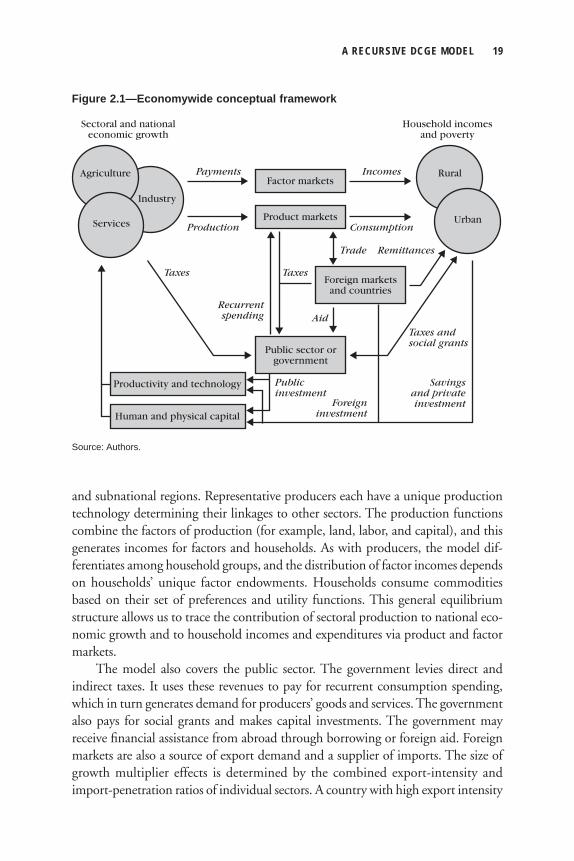
Economywide FrameworkCGE models are designed to capture the linkages between sectoral and national economic growth on the one hand and household incomes and poverty on the other (Figure 2.1). Direct and indirect transmission channels link growth to poverty, and these are largely determined by a country’s economic structure. Production-side linkages are infl uenced by sectors’ technologies. Backward production linkages arise when producers demand intermediate inputs. When agricultural production expands, it uses intermediate goods, such as fertilizers and transport, thereby stimu-lating nonagricultural production. The more input intensive a sector is, the stronger its backward linkages are. Conversely, forward production linkages account for the supply of inputs to downstream industries. When agricultural production expands, it can supply more goods to food processors, which again raises nonagricultural production.
Consumption linkages occur when household incomes are used to buy goods and services. When agricultural production expands, it raises farmers’ incomes, which are then used to purchase farm and nonfarm goods. The size of consumption linkages depends on the share of factor income distributed to households, the com-position of the consumption basket, and the share of domestically supplied goods in consumer demand. Evidence from developing countries suggests that consump-tion linkage effects are much larger than production linkage effects (that is, they account for 75–90 percent of total growth multiplier effects in Sub-Saharan Africa and 50–60 percent in Asia; see Haggblade, Hammer, and Hazell 1991). Agricultural growth multipliers are especially important in Sub-Saharan Africa (Delgado, Hopkins, and Kelly 1998).
Our model captures production and consumption linkages when evaluating economic growth. The model contains production functions disaggregated by sector
A RECURSIVE DCGE MODEL 19
and subnational regions. Representative producers each have a unique production technology determining their linkages to other sectors. The production functions combine the factors of production (for example, land, labor, and capital), and this generates incomes for factors and households. As with producers, the model dif-ferentiates among household groups, and the distribution of factor incomes depends on households’ unique factor endowments. Households consume commodities based on their set of preferences and utility functions. This general equilibrium structure allows us to trace the contribution of sectoral production to national eco-nomic growth and to household incomes and expenditures via product and factor markets.
The model also covers the public sector. The government levies direct and indirect taxes. It uses these revenues to pay for recurrent consumption spending, which in turn generates demand for producers’ goods and services. The government also pays for social grants and makes capital investments. The government may receive fi nancial assistance from abroad through borrowing or foreign aid. Foreign markets are also a source of export demand and a supplier of imports. The size of growth multiplier effects is determined by the combined export-intensity and import-penetration ratios of individual sectors. A country with high export intensity
Factor marketsAgriculture
Services
Rural
Urban
Industry
Incomes
Foreign marketsand countries
Public sector orgovernment
Remittances
Productivity and technology
Sectoral and nationaleconomic growth
Household incomesand poverty
Human and physical capital
Payments
Product marketsConsumption
TaxesTaxes
Trade
Taxes andsocial grants
Savingsand privateinvestmentForeign
investment
Recurrentspending
Publicinvestment
Aid
Production
Figure 2.1—Economywide conceptual framework
Source: Authors.
20 XINSHEN DIAO AND JAMES THURLOW
faces less stringent domestic demand constraints, whereas a higher import penetra-tion ratio means greater competition from foreign producers. The CGE model captures these interactions with the rest the world by using trade functions and tracking international transfers. Finally, our CGE model is recursively dynamic. Savings are collected into a national pool and are used to fi nance investment. Investment is converted into capital stocks to determine the rate of capital accumu-lation. Changes in factor supplies and productivity determine the overall rate of economic growth in the country. In some cases the rate of technical change is linked to the level and composition of investments.
Mathematical Specification of the ModelFollowing the tradition of general equilibrium theory, perfect competition is a key assumption in our CGE model, at least for domestic product markets. By assuming a market-based economy, our model solves for the equilibrium between demand and supply of individual factors and products, as mediated by changes in relative prices. Given the model’s multisector, multifactor, and sometimes multiregional setting, the economic structure of an economy (to which to the model is calibrated) will affect the ability of producers and consumers to respond to changing prices. Economic structure therefore infl uences changes in the distribution of incomes across household groups. The process of calibrating the model to the structure of an economy is described later in this chapter. Here we present the model specifi ca-tion using a series of mathematical equations that explain the behavioral responses of economic agents (for example, consumers, producers, and the government). Because this is a general equilibrium model, we also present equations that maintain economywide or macroeconomic consistency. We then discuss the dynamic pro-cesses of the model. The concluding section of this chapter discusses some of the model’s main limitations.
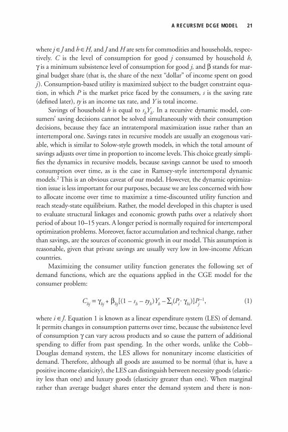
Consumer BehaviorFor a recursively dynamic model, consumer behavior is assumed to be the same as in a static model. Thus, typical consumers (and there can be more than one in the model) maximize their welfare (represented by a utility function) facing a budget constraint. Using a Stone-Geary utility function, the consumer problem can be pre-sented mathematically as:
Max∏j(Chj – γhj)βhj
subject to ∑j(Pj · Chj) = (1 – sh – tyh)Yh,
A RECURSIVE DCGE MODEL 21
where j ∈J and h ∈H, and J and H are sets for commodities and households, respec-tively. C is the level of consumption for good j consumed by household h, γ is a minimum subsistence level of consumption for good j, and β stands for mar-ginal budget share (that is, the share of the next “dollar” of income spent on good j). Consumption-based utility is maximized subject to the budget constraint equa-tion, in which P is the market price faced by the consumers, s is the saving rate (defi ned later), ty is an income tax rate, and Y is total income.
Savings of household h is equal to shYh. In a recursive dynamic model, con-sumers’ saving decisions cannot be solved simultaneously with their consumption decisions, because they face an intratemporal maximization issue rather than an intertemporal one. Savings rates in recursive models are usually an exogenous vari-able, which is similar to Solow-style growth models, in which the total amount of savings adjusts over time in proportion to income levels. This choice greatly simpli-fi es the dynamics in recursive models, because savings cannot be used to smooth consumption over time, as is the case in Ramsey-style intertemporal dynamic models.2 This is an obvious caveat of our model. However, the dynamic optimiza-tion issue is less important for our purposes, because we are less concerned with how to allocate income over time to maximize a time-discounted utility function and reach steady-state equilibrium. Rather, the model developed in this chapter is used to evaluate structural linkages and economic growth paths over a relatively short period of about 10–15 years. A longer period is normally required for intertemporal optimization problems. Moreover, factor accumulation and technical change, rather than savings, are the sources of economic growth in our model. This assumption is reasonable, given that private savings are usually very low in low-income African countries.
Maximizing the consumer utility function generates the following set of demand functions, which are the equations applied in the CGE model for the consumer problem:
Chj = γhj + βhj[(1 – sh – tyh)Yh – ∑i(Pi · γhi)]Pj
–1, (1)
where i ∈J. Equation 1 is known as a linear expenditure system (LES) of demand. It permits changes in consumption patterns over time, because the subsistence level of consumption γ can vary across products and so cause the pattern of additional spending to differ from past spending. In the other words, unlike the Cobb–Douglas demand system, the LES allows for nonunitary income elasticities of demand. Therefore, although all goods are assumed to be normal (that is, have a positive income elasticity), the LES can distinguish between necessity goods (elastic-ity less than one) and luxury goods (elasticity greater than one). When marginal rather than average budget shares enter the demand system and there is non-
22 XINSHEN DIAO AND JAMES THURLOW
zero subsistence consumption of basic commodities, then the various consumers in the model will respond differently to similar changes in incomes and market prices. For example, when household incomes rise, poor households may increase the share of their income spent on foods (that is, with an income elasticity greater than one), whereas rich households may reduce their food expenditure share (that is, with an elasticity less than one). This variation in responses explains why CGE models usually consider multiple types of consumers (or household groups), often distinguished by geographic location, rural or urban areas, income sources, or poor/nonpoor status. As discussed below, income elasticities are usually esti-mated econometrically using nationally representative household expenditure surveys.
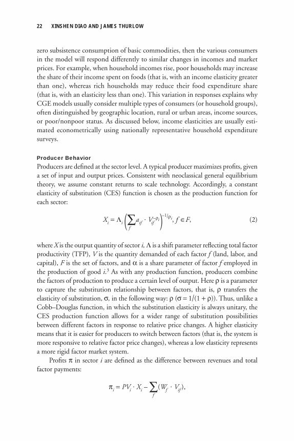
Producer BehaviorProducers are defi ned at the sector level. A typical producer maximizes profi ts, given a set of input and output prices. Consistent with neoclassical general equilibrium theory, we assume constant returns to scale technology. Accordingly, a constant elasticity of substitution (CES) function is chosen as the production function for each sector:
Xi = Λi (∑aif · Vif
–ρi)–1/ρi, f ∈F, (2) f
where X is the output quantity of sector i, Λ is a shift parameter refl ecting total factor productivity (TFP), V is the quantity demanded of each factor f (land, labor, and capital), F is the set of factors, and α is a share parameter of factor f employed in the production of good i.3 As with any production function, producers combine the factors of production to produce a certain level of output. Here ρ is a parameter to capture the substitution relationship between factors, that is, ρ transfers the elasticity of substitution, σ, in the following way: ρ (σ = 1/(1 + ρ)). Thus, unlike a Cobb–Douglas function, in which the substitution elasticity is always unitary, the CES production function allows for a wider range of substitution possibilities between different factors in response to relative price changes. A higher elasticity means that it is easier for producers to switch between factors (that is, the system is more responsive to relative factor price changes), whereas a low elasticity represents a more rigid factor market system.
Profi ts π in sector i are defi ned as the difference between revenues and total factor payments:
πi = PVi · Xi – ∑(Wf · Vif ), f
A RECURSIVE DCGE MODEL 23
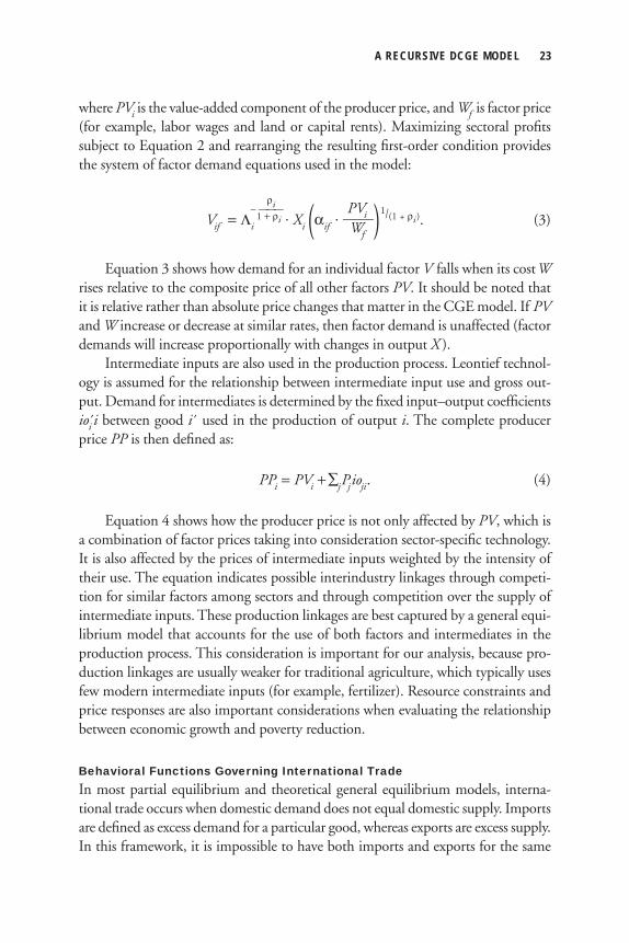
where PVi is the value-added component of the producer price, and Wf is factor price (for example, labor wages and land or capital rents). Maximizing sectoral profi ts subject to Equation 2 and rearranging the resulting fi rst-order condition provides the system of factor demand equations used in the model:
ρi – ——— PVi Vif = Λi 1 + ρi · Xi (αif
· ——)1/(1 + ρi). (3) Wf
Equation 3 shows how demand for an individual factor V falls when its cost W rises relative to the composite price of all other factors PV. It should be noted that it is relative rather than absolute price changes that matter in the CGE model. If PV and W increase or decrease at similar rates, then factor demand is unaffected (factor demands will increase proportionally with changes in output X ).
Intermediate inputs are also used in the production process. Leontief technol-ogy is assumed for the relationship between intermediate input use and gross out-put. Demand for intermediates is determined by the fi xed input–output coeffi cients ioi i between good i´ used in the production of output i. The complete producer price PP is then defi ned as:
PPi = PVi + ∑jPj ioji. (4)
Equation 4 shows how the producer price is not only affected by PV, which is a combination of factor prices taking into consideration sector-specifi c technology. It is also affected by the prices of intermediate inputs weighted by the intensity of their use. The equation indicates possible interindustry linkages through competi-tion for similar factors among sectors and through competition over the supply of intermediate inputs. These production linkages are best captured by a general equi-librium model that accounts for the use of both factors and intermediates in the production process. This consideration is important for our analysis, because pro-duction linkages are usually weaker for traditional agriculture, which typically uses few modern intermediate inputs (for example, fertilizer). Resource constraints and price responses are also important considerations when evaluating the relationship between economic growth and poverty reduction.
Behavioral Functions Governing International TradeIn most partial equilibrium and theoretical general equilibrium models, interna-tional trade occurs when domestic demand does not equal domestic supply. Imports are defi ned as excess demand for a particular good, whereas exports are excess supply. In this framework, it is impossible to have both imports and exports for the same
24 XINSHEN DIAO AND JAMES THURLOW
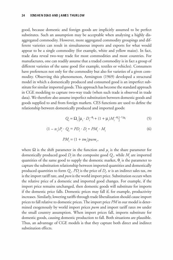
good, because domestic and foreign goods are implicitly assumed to be perfect substitutes. Such an assumption may be acceptable when analyzing a highly dis-aggregated commodity. However, more aggregated commodity groupings and dif-ferent varieties can result in simultaneous imports and exports for what would appear to be a single commodity (for example, white and yellow maize). In fact, trade data reveal two-way trade for most commodities and most countries. For manufactures, one can readily assume that a traded commodity is in fact a group of different varieties of the same good (for example, textiles or vehicles). Consumers have preferences not only for the commodity but also for varieties of a given com-modity. Observing this phenomenon, Armington (1969) developed a structural model in which a domestically produced and consumed good is an imperfect sub-stitute for similar imported goods. This approach has become the standard approach in CGE modeling to capture two-way trade (when such trade is observed in trade data). We therefore also assume imperfect substitution between domestic goods and goods supplied to and from foreign markets. CES functions are used to defi ne the relationship between domestically produced and imported goods:
Qi = Ωi [μi · Di
– θi + (1 + μi)Mi– θi]–1/θi (5)
(1 – tci)Pi · Qi = PDi
· Di + PMi · Mi (6)
PMi = (1 + tmi)pwmi ,
where Ω is the shift parameter in the function and µi is the share parameter for domestically produced good Di in the composite good Qi , while Mi are imported quantities of the same good to supply the domestic market, θi is the parameter to capture the substitution relationship between imported quantities and domestically produced quantities to form Qi , PDi is the price of Di, tc is an indirect sales tax, tm is the import tariff rate, and pwn is the world import price. Substitution occurs when the relative price of a domestic and imported good changes. For example, if the import price remains unchanged, then domestic goods will substitute for imports if the domestic price falls. Domestic prices may fall if, for example, productivity increases. Similarly, lowering tariffs through trade liberalization should cause import prices to fall relative to domestic prices. The import price PM in our model is deter-mined exogenously by world import prices pwm and import tariff rates tm under the small country assumption. When import prices fall, imports substitute for domestic goods, causing domestic production to fall. Both situations are plausible. Thus, an advantage of CGE models is that they capture both direct and indirect substitution effects.
A RECURSIVE DCGE MODEL 25
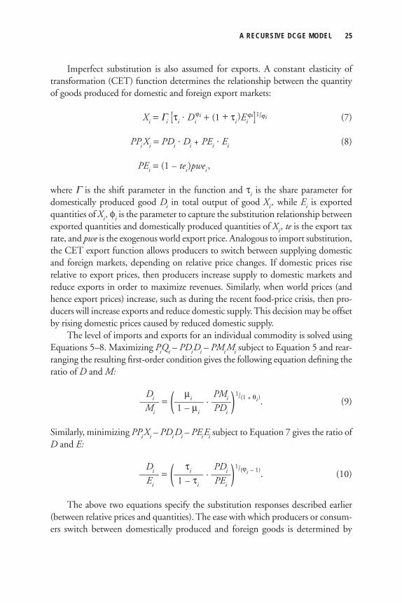
Imperfect substitution is also assumed for exports. A constant elasticity of transformation (CET) function determines the relationship between the quantity of goods produced for domestic and foreign export markets:
Xi = Γi [τi · Diϕi + (1 + τi
)Eiϕi]1/ϕi (7)
PPi Xi = PDi · Di + PEi · Ei (8)
PEi = (1 – tei)pwei ,
where Γ is the shift parameter in the function and τi is the share parameter for domestically produced good Di in total output of good Xi, while Ei is exported quantities of Xi, φi is the parameter to capture the substitution relationship between exported quantities and domestically produced quantities of Xi, te is the export tax rate, and pwe is the exogenous world export price. Analogous to import substitution, the CET export function allows producers to switch between supplying domestic and foreign markets, depending on relative price changes. If domestic prices rise relative to export prices, then producers increase supply to domestic markets and reduce exports in order to maximize revenues. Similarly, when world prices (and hence export prices) increase, such as during the recent food-price crisis, then pro-ducers will increase exports and reduce domestic supply. This decision may be offset by rising domestic prices caused by reduced domestic supply.
The level of imports and exports for an individual commodity is solved using Equations 5–8. Maximizing PiQi – PDiDi – PMiMi subject to Equation 5 and rear-ranging the resulting fi rst-order condition gives the following equation defi ning the ratio of D and M:
Di μi PMi —— = (——— · ——)1/(1 + θi). (9) Mi 1 – μi PDi
Similarly, minimizing PPi Xi – PDiDi – PEiEi subject to Equation 7 gives the ratio of D and E:
Di τi PDi —— = (——— · ——)1/(ϕi – 1). (10) Ei 1 – τi PEi
The above two equations specify the substitution responses described earlier (between relative prices and quantities). The ease with which producers or consum-ers switch between domestically produced and foreign goods is determined by
26 XINSHEN DIAO AND JAMES THURLOW
elasticities of substitution θ and φ. Larger elasticities permit greater responsiveness to relative price changes. These elasticities can be estimated based on historical quantity–price relationships using econometrics or back-casting techniques (see, for example, Arndt, Robinson, and Tarp 2002).
Equilibrium Conditions A key difference between partial and general equilibrium models is the determina-tion of prices. In most partial equilibrium models, prices are either exogenously given or determined by predefi ned price functions. In general equilibrium theory, all factor and commodity prices are determined endogenously by market equilib-rium conditions. Without international factor mobility, factor prices W are fully endogenous. To simplify our discussion, we initially assume that all factors are fully employed and mobile across sectors. This implies the following factor market equilibrium condition:
∑Vif = V Sf , (11) i
where V Sf is the total factor supply and Vif is factor demand in each sector (deter-mined in Equation 3). Total factor supply is fi xed in any given year. Any changes to V Sf must be determined exogenously or independently of the forces infl uencing Vif . Equation 11 determines factor returns Wf , which are therefore affected by sector-level factor demands and the total supply of each factor.
The second key feature distinguishing general equilibrium models is their treat-ment of household incomes, which, via the budget constraint, determines consumer demand for individual commodities. Partial equilibrium models often treat income as an exogenous variable or something determined by forces other than the produc-tion system. In general equilibrium models, income is generated from the returns earned by factors (and by remittance transfers, when they exist). To simplify our discussion, we assume all factors are owned by households,4 such that household income Y is determined by
Yh = ∑δhf (1 – tff )Wf · Vif , (12) if
where δ is a coeffi cient matrix that sums to one and determines the distribution of factor earnings among individual households. Direct taxes tff are imposed on total factor V Sf ’s earnings (for example, corporate taxes on capital profi ts). The distribu-tion of factor incomes is determined by households’ factor endowments. For exam-ple, higher income households are usually better endowed with capital and skilled
A RECURSIVE DCGE MODEL 27
labor, and so these households receive the most capital profi ts and a larger share of skilled labor’s wage income than do lower income households. The value of δ is therefore the driving factor behind distributional outcomes in our model. As dis-cussed in the next subsection, information on household income sources is drawn from household survey data.
Domestic prices are determined by equilibrium conditions in the product market. As foreign demand and exports are determined in Equations 9 and 10, market equilibrium can be defi ned in terms of the composite good Q instead of D as follows:
Qi = ∑Cih + Ni + Gi + ∑j(ioji · Xi), (13)
h
where N is investment demand and G is government recurrent consumption spend-ing (both defi ned later). Changes in right-hand-side variables in Equation 13 refl ect shifts in demand, whereas changes in Q represent changes in supply. When changes in total demand and supply are unequal, then domestic prices PD, and hence P, change to establish a new market equilibrium.
The relationship between savings and investment demand N, and taxes and government spending G, will be specifi ed below. However, in the absence of taxes or savings (that is, when ty, tf, s, N, and G are all zero), the above 13 equations simultaneously solve for the values of the 13 endogenous variables (Y, C, X, V, Q, D, M, E, P, PV, PP, PD, and W ). The general equilibrium solution defi ned by the equations only holds if there are no foreign transfers, implying a zero trade bal-ance. This assumption is often made in simple theoretical general equilibrium models, but it is rarely used in CGE models, which need to be calibrated to observed data for a country. Later we introduce foreign transfers and current account im-balances. Before doing this, however, we fi rst defi ne government G and investment demand N.
Government and Investment DemandThe government in our CGE model appears as a separate institution with incomes and expenditures but without any behavioral functions. In other words, its decision to either consume or invest is not solved as an optimization problem. Total domestic revenues R is the sum of all individual taxes:
R = ∑(tci · Pi · Qi + tmi · pwmi
· Mi + tei · pwei · Ei) + (14)
i
∑(tyh · Yh) + ∑f (tff · Wf · V Sf ).
h
28 XINSHEN DIAO AND JAMES THURLOW
Tax rates are typically exogenous in a CGE model so that they can be used to simulate policy changes. The government may also receive income from abroad, such as via foreign grants or borrowing and from holding assets. These additional income sources are discussed below when we introduce macroeconomic closure.
Tax rates are typically exogenous in a CGE model so that they can be used to simulate policy changes. Although the government does not attempt to maximize revenues by endogenously changing tax rates, its revenues increase at given tax rates when the economy grows. This allows the government to increase savings and investment, create more public goods, and enhance productivity for the private sector. African governments usually receive additional nontax income from abroad, such as via foreign grants /borrowing and from holding assets. These additional income sources are treated as exogenous to the model and are discussed below when we introduce macroeconomic closure.
The government uses its revenues to purchase goods and services (that is, recur-rent consumption spending) and to save (that is, fi nance public capital investment):
R = ∑(Pi · Gi) + FB, (15) i
where G is consumption spending from Equation 13 and FB is the recurrent fi scal balance, which can be positive to represent surplus and negative to represent defi cit. Because we do not have behavioral functions that optimize revenues and expendi-tures, our model does not endogenously balance government accounts. Rather, we assume that G is determined exogenously, implying that an increase in government revenues causes the fi scal surplus (or public savings or investment) to expand (or the defi cit to contract). The fi scal balance FB is therefore merely a residual balancing item. In reality, the government also makes transfers to (and receives incomes from) households and fi rms (such as social grants and contributions). Such transfers are captured in the model as either fi xed values or in proportion to changing household populations or incomes. Although such transfers are considered in the CGE model, we exclude them here to simplify the equations.
There is also no behavioral function determining the level of investment demand for goods and services (N from Equation 13). The total value of all invest-ment spending must equal the total amount of investible funds I in the economy. We therefore assume that the value of N for each good i is in fi xed proportion to the total value of investment:
I · εi = Pi · Ni, (16)
where ε is the value share for each good i and P is the market price determined by the equilibrium condition in Equation 13. To determine the value of I we must defi ne the macroeconomic closure.
A RECURSIVE DCGE MODEL 29
Current Account and Macroeconomic ClosureMacroeconomic balance in a CGE model is determined by a series of closure rules. The most important of these is for the current account balance. Neoclassical general equilibrium theory does not permit current account imbalances. How-ever, CGE models are often calibrated to observed data for a country, where current accounts are invariably imbalanced. Thus, our model will not be able to achieve equilibrium unless we include external fi nancial fl ows, such as incomes from hold-ing foreign assets or the government’s external borrowing or foreign aid receipts. Current account imbalances must be accounted for, because they affect the real economy via the relationship between exports and imports and between savings and investment. To incorporate these considerations into our model, we start from the well-known identity linking a country’s current account balance CA to national savings S and investment I:
CA = TE – TM – NFI = S – I = ΔNFA, (17)
where TE = ∑(pwei · Ei) and TM = ∑(pwmi · Mi). i i
The left-hand side of the identity states that a country’s current account balance is equal to its trade balance (TE –TM) less net foreign incomes NFI. A country is therefore running a current account surplus when the sum of its trade balance and NFI is positive, in which case national savings exceed national investment and there is an accumulation of net foreign assets NFA. Total savings in the economy is the sum of all household savings and the government’s recurrent fi scal balance:
S = ∑( sh · Yh) + FB. (18) h
Before discussing the adopted closure rules, we must fi rst expand two previous equations to include the foreign transfers received by households and the govern-ment (that is, the components of NPI ). We rewrite Equations 12 and 15 as:
Yh = ∑(δhf (1 – tff )Wf · Vif ) + hwh (12´) if
R + rw = ∑(Pi · Gi) + FB, (15´) i
where hw are foreign transfers received by households (for example, remittances) and rw are incomes earned by the government (for example, foreign aid). If transfers are negative, then they denote net foreign payments (such as interest paid on foreign
30 XINSHEN DIAO AND JAMES THURLOW
debt). Given these new Equations 12´ and 15´, the value of NFI in Equation 17 can be defi ned as
NFI = ∑ hwh + rw. i
We cannot model hw and rw endogenously, because they are determined by the workings of the global economy and our model is only for a single country. These two variables (and hence NFI) are therefore exogenous in the model. The current account balance CA may not be equal to NFI if there is a trade surplus or defi cit observed in the country’s data. When CA is greater (less) than NFI, the country runs a trade surplus (defi cit), and total exports are greater (less) than total imports plus NFI. For the external account, the fi rst closure rule is to treat the cur-rent account balance CA as an exogenous variable, thus controlling its effect on the macroeconomic behavior of the model. For a given level of CA, the level of total exports and imports can change, but they have to change simultaneously. For example, CGE models are often used to simulate trade liberalization. Reducing import tariffs affects relative prices for different commodities, which in turn affects imports and exports at the sector and national levels. In this case, total imports usu-ally increase at a given CA, which then affects relative prices and exports at the sector level. At the national level, total exports have to increase in response to rising imports to maintain CA.
The choice of current account closure infl uences how we select the second closure rule, which is the identity on the right-hand side of Equation 17. By fi xing CA, we are also fi xing the value of ΔNFA, which means that either total savings S or total investment I (but not both) should be determined exogenously. We call this choice the “savings–investment” closure, which is a term borrowed from macro-economics. If the CGE model is savings driven, then I is automatically determined by the level of total available savings (that is, I = S – ΔNFA). Consistent with Equation 1, in which s is a fi xed parameter, our model specifi cation is savings driven. Finally, our treatment of the government balance in Equation 15´ is in fact the third closure rule in the model. We choose to make recurrent consumption spend-ing G exogenous and allow the fi scal balance FB to adjust to changes in revenues R.
Through the introduction of the government, investment demand, and macro-economic closures, we have included fi ve new equations into the model (Equations 14–18) and fi ve new endogenous variables (R, FB, N, I, and S).5 Together, the 18 equations and variables describe a static single-country model. Our current account closure fi xes the national trade balance. The government closure implies that chang-es in revenues alter the fi scal balance (and hence public investment). In our savings-driven closure, total investment adjusts to match total savings. To determine the
A RECURSIVE DCGE MODEL 31
lasting consequences of changing investment levels, we have to introduce dynamics into the model.
Recursive Dynamics Most CGE models are essentially static in nature. As mentioned earlier, consumers’ demands are derived from a one-period utility function. Saving rates are not en-dogenously determined by an intertemporal utility function, and so they are not used to smooth consumption over time. Investment and capital accumulation rates are therefore not intertemporally determined either. Rather, the dynamics in our CGE model is defi ned as a recursive process. Thus, we can completely separate the model into within-period and between-period components.6 The equations pre-sented above fully specify the within-period component, in which consumers and producers maximize their utility and profi ts based on prevailing factor and product prices (that is, without forward-looking expectations). Then, between periods, certain exogenous variables in the static model are updated based on either externally determined trends or previous period results. We describe these two kinds of updating procedures in turn.
Various external trends are imposed on the model. Although not shown in Equations 1–18, each variable in the model has a time subscript associated with it. The two most important trends are changes in factor supplies (a proxy for popula-tion) and productivity, which are represented by VS in Equation 11 and Λ in Equation 2. The fi rst two dynamic equations update these exogenous variables:
V Sf t + 1 = V Sf t(1 + gvft), where f ≠ k (19)
Λit + 1 = Λit(1 + gpit) (20)
Git + 1 = Git(1 + ggit), (21)
where t is the time subscript in the simulation period (for example, years), k is a subset of f containing the capital factor, gv is the change in supply for factor f in period t, gg is the rate of change in recurrent government spending, and gp is the change in sector i ’s production function’s shift parameter (that is, TFP) in period t. Capital supply is excluded from Equation 19, because, as discussed below, it is based on previous period results. Population growth enters the model via changes in labor supply. However, with nonunitary income elasticities (that is, unequal marginal and average budget shares), consumer demand in Equation 1 must be re-specifi ed in per capita terms. Equation 21 shows how government consumption spending G is updated every period based on exogenous trends in is the rate of change in recurrent government recurrent spending gg. All other parameters in the
32 XINSHEN DIAO AND JAMES THURLOW
model are fi xed values. These include, for example, tax or saving rates (ty, s, respec-tively), share parameters (β), and foreign transfers (FS, hw, and rw).
Between-period updating may also be based on results from the previous period. Sectoral capital accumulation rates are endogenously determined in the model based on investment levels from the previous period. The amount of new capital is determined by dividing total investment I by the capital goods price. This amount is added to existing capital stocks after adjusting for depreciation. Assuming only a single type of capital that is mobile across sectors, as in the model specifi ed above, then the following equation captures the capital accumulation process:
It VSkt + 1 = (1 – d )VSkt + ——, where PKt = ∑ Pitεi , (22)
PKt i
where d is the national depreciation rate, PK is the capital goods price, and ε is the value share for each good i in the total investment basket from Equation 16. Because k is mobile, new capital is allocated endogenously to equilibrate capital returns across sectors.
In reality, capital is not as mobile as other factors, such as labor, and so we make it immobile across sectors after it has been invested. This assumption implies that the returns on capital in each sector no longer have to be equal. We therefore attach a sector-specifi c distortion term Z in front of the economy-wide factor return variable W in Equations 3, 12, and 14. Equation 3 is now replaced by
ρi – ——— PVi Vif = Λi 1 + ρi · Xi (αif
· ————)1/(1 + ρi), for f = k, (3´) Zif · Wf
where Z is an adjustment factor (0 < Z < ∞) and is initially set equal to one. An increase in capital demand in a sector causes Z to rise above one, and vice versa. Similarly, we replace Equation 22 with a capital stock updating equation defi ned at the sector level (that is, in terms of V instead of VS):7
It Vikt + 1 = (1 – d )Vikt + SKikt · ——. (22´)
PKt
The term SK in Equation 22´ is the new capital allocation parameter (0 < SK < 1) and specifi es how much investment is directed toward each sector. The sum of the SK factors therefore equals one. We follow the approach of Dervis, de Melo, and Robinson (1982) by defi ning SK as:
A RECURSIVE DCGE MODEL 33
SRikt – ARt SKikt = SPikt + ω · SPikt (—————), (23) ARt
where SP is the current sectoral share in aggregate profi ts, SR is the sectoral profi t rate (equal to ZifWf ), AR is the economywide average profi t rate, and ω is an invest-ment mobility parameter. In this simple specifi cation, new capital is allocated in proportion to each sector’s share in aggregate capital income, adjusted by the sector’s profi t rate relative to the average profi t rate.8 Sectors with higher than average profi t rates receive a larger share of investible funds than their share in aggregate profi ts. Note that the specifi cation in Equation 23 allows us to drop the assumption of only a single type of capital in the set F. This investment allocation procedure is known as a “putty-clay” specifi cation, because new capital is mobile, but once invested it becomes sector specifi c. More detailed descriptions of the model parameters, vari-ables, and equations can be found in Tables 2A.1 and 2A.2.
The above discussion presents our core CGE model. In summary, the CGE model describes the interactions of various agents, such as households, producers, and the government, in a market-based economy. We capture sectors’ technologies via input coeffi cients, and we allow these to adapt to relative price movements by allowing imperfect substitution in the production and trade functions. While cap-turing the structure and behavior of individual representative households, we main-tain the macroconsistency of microlevel decisionmaking through our general equilibrium framework. The next two sections summarize the model specifi cation in more accessible language and then describe how it is calibrated to empirical data. However, we conclude this subsection by describing some features of the model that were not shown in the above equations.
Regional Production and Marketing Costs We extend the core CGE model described above in two areas.9 First, we introduce marketing margins or transaction costs into the model, so that there is a wedge between producer prices PP and market prices P. These transaction costs are imposed on domestic, exported, and imported goods, and they generate demand for the domestic trade and transport services sectors (see Lofgren, Harris, and Robinson 2001).
Second, we disaggregate production across subnational regions (that is, the variables X, Z, PP, and V have regional subscripts). All regional producers have their own production functions and technology coeffi cients, and they often use region-specifi c factors, such as agricultural land and farm labor. All regional producers supply their output to a national product market, which avoids having to model interregional trade fl ows that are usually diffi cult to measure. Output from each region is combined into a composite national good using a CES aggregation func-
34 XINSHEN DIAO AND JAMES THURLOW
tion. Although a single national price exists for each commodity, producers may incur region-specifi c transaction costs when supplying the national market. Producer prices therefore vary across regions. We also disaggregate households by region, although this is done by calibration rather than by the use of regional subscripts.
These two extensions to the core model allow us to refl ect spatial heterogeneity in geographic conditions and marketing constraints. These considerations are important for developing countries, where markets are often underdeveloped, and for agriculture, which depends on agroecological and climatic conditions.
Calibrating the Model to Country DataOne of the main advantages of CGE models over (more complex) theoretical mod-els is their calibration to detailed empirical data. “Calibration” refers to the process of assigning values to the model’s parameters and variables, typically using observed country data. Some of the assumptions made when specifying the CGE model were done to ease its calibration, because in many cases the data needed for more complex functional forms are unavailable in developing countries. For example, the LES func-tion used to determine consumer demand assumes that income elasticities remain constant. More elaborate functions often drop this assumption, such as in the “almost ideal demand system.” However, we retain the LES function, because it requires data that can readily be obtained from household surveys (for example, expenditure shares and income elasticities). Calibrating the behavior of more com-plicated functional forms often just involves making more assumptions where data are unavailable. This section describes the data sources and estimation procedures used to calibrate our CGE models.
Social Accounting MatrixesThe values of almost all variables and parameters in the CGE model are drawn from a social accounting matrix (SAM).10 Constructing a SAM is therefore a fundamental part of developing a CGE model. A SAM is an economywide representation of a country’s economic structure. It captures all income and expenditure fl ows among producers, consumers, the government, and the rest of the world during a particular year. Table 2.1 presents the structure of a SAM that could be used to calibrate the core model described above. The SAM contains a number of “accounts” representing dif-ferent agents in the model, including sectors (producers) and households (consumers). The rows and columns of the SAM represent incomes and payments, respectively, from one account to another. As with double-entry accounting, the SAM is a consis-tent economywide database, because row and column totals must be equal. In other words, a payment from one account always becomes an income for another. The SAM therefore provides the base-year equilibrium state for the CGE model.
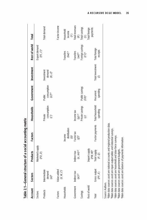
A RECURSIVE DCGE MODEL 35
Tabl
e 2.1—
Gene
ral s
truct
ure o
f a so
cial a
ccou
ntin
g m
atrix
Acco
unt
Sect
ors
Prod
ucts
Fa
ctor
s Ho
useh
olds
Go
vern
men
t In
vest
men
t Re
st o
f wor
ld
Tota
lSe
ctors
Ma
rketed
supp
ly
Ex
port
dema
nd
(PD,
D)
(P
E, E
)a Pr
oduc
ts Int
erme
diate
Pr
ivate
Publi
c Inv
estm
ent
To
tal de
mand
dema
nd
co
nsum
ption
cons
umpti
on
de
mand
(io
)b
(C)c
(G
)b,d
(N
, ε)b
Fa
ctors
Value
-add
ed
Facto
r inco
me
(V
, W, Z
)c
Hous
ehold
s
Inc
ome
Tr
ansfe
rs Ho
useh
old
dis
tributi
on
(hw)
c,e
inc
ome
(δ)c
(Y
)Go
vern
ment
Indire
ct tax
Ind
irect
tax
Facto
r tax
Inc
ome t
ax
Tran
sfers
Total
reve
nues
(te)a,d
(tc, tm
)a,d
(tf
)d
(ty)c,d
(rw)d,e
(R)
Savin
gs
Pr
ivate
savin
gs
Publi
c sav
ings
Fo
reign
savin
gs
Total
savin
gs
(s)c
(FB)
d
(F
S)e
(S
)Re
st of
world
Impo
rt su
pply
Total
fore
ign
(PM
, M)a
paym
ents
Total
Gr
oss o
utput
To
tal su
pply
Facto
r pay
ments
To
tal ho
useh
old
Recu
rrent
Total
inve
stmen
t To
tal fo
reign
(PP,
X)
(P
, Q)
spen
ding
sp
endin
g
(I)
re
ceipt
s
Sour
ce: A
uthor
s.a Ma
in da
ta so
urce
s use
d are
natio
nal a
ccou
nts an
d reg
ional
prod
uctio
n data
.b Ma
in da
ta so
urce
s use
d are
inpu
t–outp
ut tab
les an
d ind
ustria
l sur
veys
.c Ma
in da
ta so
urce
s use
d are
hous
ehold
and l
abor
force
surve
ys.
d Main
data
sour
ces u
sed a
re go
vern
ment
budg
ets.
e Main
data
sour
ces u
sed a
re ba
lance
of pa
ymen
ts inf
orma
tion.
36 XINSHEN DIAO AND JAMES THURLOW
A SAM is constructed in two stages. During the fi rst stage, data from different sources are entered into each of the SAM’s cells. As with the CGE model, the SAM allows for multiple sectors and households. Thus, the sector, product, and house-hold rows and columns actually contain many subaccounts. The three main data sources for constructing a SAM are national accounts, input–output tables (or supply–use tables), and nationally representative household budget surveys. As shown in Table 2.1, national accounts provide information on the composition of GDP at factor cost (that is, sectoral value-added) and by broad expenditure groups at market prices (for example, C + I + G + E – M). The technical coeffi cients in the input–output table are used to estimate intermediate demand based on sectors’ levels of GDP or gross output. It also disaggregates government and investment demand across products. The household survey is used to segment labor markets (that is, disaggregate labor income into different groups, such as by education). The survey also defi nes households’ expenditure patterns and the distribution of factor incomes to representative household groups. The survey data are therefore the main determinant of differential income and distributional effects across household groups in the CGE model.
Other databases are used to complete specifi c cells in the SAM. Government budgets provide information on tax rates, revenues, and expenditures. Although not shown in the table, government budgets (and household surveys) also deter-mine the level and distribution of social transfers. Customs and revenue authorities provide data on imports and exports and their associated tariffs and subsidies. The balance of payments, usually compiled by a country’s central bank, is used to popu-late the external or “rest of world” account, including information on transfer receipts and payments and the current account balance. Finally, sectors in our SAMs are usually disaggregated across subnational regions using information on regional production and technologies from agricultural and industrial surveys. Trade margins, which are not shown in the table, are estimated using information on producer and consumer prices. Trade margins may also be drawn from input–output or supply–use tables.
There are inevitably inconsistencies between data from different sources, which lead to unequal row and column totals in our SAMs. The second stage of construct-ing a SAM is therefore to balance these totals. This reconciliation of data from disparate sources is similar to a rebasing of national accounts. We use cross-entropy econometric techniques to estimate a balanced SAM (see Robinson, Cattaneo, and El-Said 2001). This procedure is a Bayesian approach that uses a cross-entropy distance measure to minimize the deviation in the balanced SAM from the un-balanced SAM containing the original data. Constraints are imposed during the estimation procedure to refl ect narrower confi dence intervals around better-known control totals (for example, total GDP). Table 2.1 shows which cell entries in the
A RECURSIVE DCGE MODEL 37
balanced SAM are used to calibrate the model’s variables and parameters. From this table it is clear that the SAM and its underlying data sources provide almost all the information needed to calibrate the CGE model. Only the behavioral elasticities remain (β, ρ, θ, and ϕ).
Behavioral Elasticities and Other External DataBehavioral elasticities are needed for the consumption, production, and trade func-tions. The LES demand function requires information on income elasticities and the Frisch parameter (see Frisch 1959). We econometrically estimate income elastici-ties using the same household survey data on which the SAM is built, following the approach described in King and Byerlee (1978). Marginal budget shares (β in Equation 1) are derived by combining the estimated income elasticities with the average budget shares drawn directly from the SAM.
Trade elasticities determine how responsive producers and consumers are to changes in relative prices when deciding to supply goods to or purchase goods from foreign markets. Higher elasticities are expected when substituting between more homogenous products, such as maize and copper. Lower elasticities are expected for more differentiated product categories, such as chemicals and machinery. In most developing countries the data needed to econometrically estimate country-specifi c elasticities do not exist—not, at least, in an appropriate form (see Arndt, Robinson, and Tarp 2002). We therefore assign values to our two trade elasticities (θ and ϕ in Equations 5 and 7) using global estimates from Dimaranan (2006).
The elasticities governing factor substitution in the production functions (ρ in Equation 2) rarely exist for developing countries. In the absence of reliable country-specifi c estimates, we assume elastic factor substitution for most activities (that is, σ > 1: σ is a transformation of ρ). This assumption is consistent with recent meta-analyses of econometrically estimated elasticities (see, for example, Boys and Florax 2008) and cross-country econometric analysis (see Behar 2009).
Finally, the SAM provides information on values but not on quantities. We therefore use external data sources to calibrate the model’s production output X and factor quantities V. For example, crops’ land use and gross output are calibrated to match agricultural data on harvested area (in hectares) and production quantities (in metric tons). Observed labor employment numbers are also used to determine sector-specifi c wages (Z in Equation 3´). In such cases, factor and product prices in the model are not normalized to one, but rather refl ect observed prices.
Baseline Dynamics The model is calibrated to the base year refl ected in the SAM. It is then run forward over time to create a baseline growth path—normally a series of years. The baseline scenario is therefore determined by annual growth in factor supplies and produc-
38 XINSHEN DIAO AND JAMES THURLOW
tivity. The growth rates of factor supplies (apart from capital) and productivity are calibrated to observed historical trends. For example, changes in labor supply are usually based on population projections for rural and urban areas and on labor force participation rates for workers with different education levels. Similarly, agricultural land either expands alongside rural population or is calibrated to long-term trends in total harvested land area from historical data. The annual growth capital stocks are targeted so that they grow at a relatively smooth rate in relation to GDP. This is done either by assigning base-year capital–output ratios or by adjusting the price of capital PK.
After a suitable baseline scenario has been calibrated, it is possible to conduct counterfactual simulations. Alternative growth paths are evaluated by changing exogenous variables in the model from baseline levels. The model is re-solved, and deviations from the baseline are attributed to the simulated change in policies or external factors. The model is therefore an ideal tool for ex ante evaluation of devel-opment options in countries where historical evidence is lacking and ex post analysis is impossible. Even though the model’s general equilibrium specifi cation is based on economic theory, its detailed calibration to observed data provides a quasi-empirical laboratory for conducting complex experiments within a consistent modeling framework.
Linking to Poverty and Nutrition ModulesThe household survey provides detailed information on the income and expenditure fl ows of individual respondents. Some of this information is lost when it is aggre-gated into representative households in the CGE model. To retain as much informa-tion as possible, we link each representative household in the model to its cor-responding household in the survey. Changes in household consumption quantities in the model are passed down to the survey and used to update the consumption levels of corresponding respondents:
Ciht HHhist = HHh
ist – 1 · ———, where g:s → h, (24) Ciht – 1
where s is the survey’s detailed household, C is the quantity of aggregate commodity i consumed by representative household h in the model (see Equation 1), and HH is the quantity of detailed commodity i consumed by household s in the survey. g represents the mapping relationship between survey's detailed households and the more aggregate households in the CGE model (a many-to-one mapping). Equation 24 shows how annual consumption changes in the model cause proportional changes
A RECURSIVE DCGE MODEL 39
for corresponding survey households. We therefore assume that all survey house-holds in a group experience the same proportional change in consumption. However, the different consumption patterns of survey households mean that changes in total consumption levels will vary across households in each group:
HTs = ∑i(HHis · psis), (25)
where HT is total consumption of the survey household s and ps is the price of com-modity i paid by household s. We fi x ps at base-year levels (or normalize it to one if price and quantity data are not identifi ed separately in the survey), so that HT refl ects real consumption changes. We compare HT to base-year poverty lines to determine whether a survey household is classifi ed as poor or nonpoor in each time period and simulation. From this we can calculate standard poverty measures.11 Our poverty module is top-down: we do not impose consistency in absolute consump-tion changes between the CGE model and the microsimulation module. It is also expenditure based, because consumption changes rather than factor income changes are passed down to the survey.12
A similar top-down approach is used to estimate changes in households’ nutri-tional status. Consumption quantity data from the household survey is combined with calorie tables to calculate initial caloric availability. As with Equations 24 and 25, model results on changes in food consumption quantities are then applied to the survey data to estimate changes in total household caloric availability adjusted by adult equivalence scales (see UNU, WHO, and FAO 2004). This measure is compared to a “malnutrition line” to determine changes in calorie-defi ciency rates for each time period and simulation. The nutrition module retains the detailed information in the household survey and accounts for size and demographic struc-ture when determining the minimum number of calories required by each household.
Summary of the Model As discussed in this chapter, an important factor determining the contribution of sectors to economywide growth is their linkages to the rest of the economy. For example, agriculture’s proponents argue that agriculture has strong growth linkages. Both consumption (forward) and production (backward) linkages are captured in our CGE model, whose nested CES production functions allow producers to gener-ate demand for both factors and intermediates when maximizing profi ts. To refl ect the heterogeneity of producers, our models are calibrated to detailed SAMs that distinguish among multiple sectors, regions, and products. Products are traded
40 XINSHEN DIAO AND JAMES THURLOW
within national markets (that is, the model does not capture trade fl ows among subnational regions). The CGE model identifi es multiple types of factors, including capital, labor, and cropland. Land and labor are usually disaggregated across skill groups and subnational regions. Both land and labor can be reallocated or migrate across sectors in response to endogenously determined factor demands. In contrast, capital is immobile and earns sector- or region-specifi c returns. This detailed speci-fi cation of production and factor markets in our model allows us to capture the changing scale and technology of production across sectors and subnational regions, and therefore can demonstrate how changes in the structure of growth will infl uence a country’s distribution of incomes and household poverty.
The contribution of different sectors to economic growth is infl uenced by international trade. For example, some development specialists are skeptical about agriculture’s role in development. They suggest that import competition has under-mined agriculture’s growth linkages and that the availability of food imports reduces the need for investment in domestic agriculture. Furthermore, in agriculture, there are greater market opportunities for export crops than for food staples. Our CGE model captures both import competition and export opportunities by allowing producers and consumers to shift between domestic and foreign markets, depending on changes in the relative prices of imports, exports, and domestic goods. More specifi cally, the decision by producers to supply domestic or foreign markets is governed by CET functions, whereas the decision to purchase domestically pro-duced or imported products is determined by CES functions. In this way the CGE model captures how import competition and the changing export opportunities of different sectors can strengthen or weaken the linkage between their economic growth and the resultant poverty reduction.
The relative importance of sectors in improving household livelihoods may vary considerably. Income and expenditure patterns differ across households, especially across subnational regions and rural and urban areas. These differences are impor-tant for distributional change, because the incomes generated by different sectors will accrue to different households, depending on their location and factor endow-ments. To capture this process, the CGE model distinguishes among various repre-sentative households, each of which is an aggregation of a group of households in nationally representative household surveys. Households in the model earn incomes through the employment of their factors of production; they then pay taxes, save, and make transfers to other households. Each household uses its remaining income to consume commodities under an LES demand system. To retain as much informa-tion on households’ income and expenditure patterns as possible, the CGE model is linked to a microsimulation module based on a national household survey. Changes in commodity consumption for each aggregate household group in the
A RECURSIVE DCGE MODEL 41
CGE model are used to adjust the commodity-level expenditures of corresponding households in the survey. Real consumption levels are then recalculated in the sur-vey, and standard poverty measures are re-estimated using the revised consumption measure.
The CGE model makes several assumptions about how the overall economy maintains macroeconomic balance. These closure rules concern the current account, the government’s fi scal balance, and the savings or investment account. We essen-tially assume that a real exchange rate adjusts to maintain a fi xed current account balance. Thus, our model countries cannot increase foreign borrowing but have to generate export earnings to fi nance imports. Although this assumption realistically limits the degree of import competition in the domestic market, it also underlines the importance of export-oriented sectors, such as high-value agriculture. For the government account, tax rates and consumption expenditures are determined exo-genously, leaving the fi scal balance to adjust to ensure that public revenue equals spending. Finally, we assume that total investment adjusts to changes in national savings under a closure rule for savings-driven investment. These fi nal two closures allow the model to capture the negative crowding-out effects of falling government revenues when the structure of growth shifts toward lower tax-paying sectors, such as traditional agriculture.
The CGE model is recursive dynamic, which means that certain parameters are updated between periods based on historical trends or results from the previous period. Our models are generally run for 10–15 years, with each equilibrium period representing a single year. During this time the model captures exogenous demo-graphic and technological changes. Changes in the population, labor supply, human capital, and TFP are drawn from historical trends. Capital accumulation is deter-mined endogenously, with previous-period investment generating new capital stock. Although the allocation of new capital is infl uenced by sectors’ or regions’ current shares of gross operating surplus, the fi nal allocation depends on depreciation and relative profi tability. Sectors generating above-average returns in the previous period will receive a larger share of new capital in the current period.
In summary, the CGE model incorporates distributional change by (1) dis-aggregating growth across sectors and subnational regions, (2) capturing employ-ment effects through factor markets and price effects through product markets, and (3) translating these two effects onto each household in the survey according to the household’s unique factor endowment and income and expenditure patterns. The structure of the growth–poverty relationship is therefore defi ned explicitly ex ante based on observed country-specifi c structures and behavior. This defi nition allows for the model to capture and contrast the distributional outcomes associated with economic growth in different sectors.
42 XINSHEN DIAO AND JAMES THURLOW
Limitations of the Model
Data ConstraintsEven though CGE models address some of the limitations of other ex ante modeling approaches, they are not without their own limitations. To begin with, they are very data intensive, which is perhaps the most common criticism lodged against CGE models. To calibrate the model, it is necessary to construct a SAM, which draws together information from a wide range of data sources. Often these data are in-consistent and are imprecisely measured. This problem is obviously a constraint for most methodologies. However, the process of reconciling a SAM inevitably causes damage to all data sources. Without knowing the relative merits of each source, it is impossible to determine whether important information is lost in the SAM esti-mation process. Because most parameter values for CGE models are drawn from SAMs and economic structure is a key determinant of simulation results, low-quality data and poor SAM estimation procedures can greatly undermine the empirical strength of CGE analysis.
Data concerns are almost impossible to fully address, because errors exist in every economic instrument or measure. Moreover, data on developing countries are often of lower quality than elsewhere, which further complicates attempts to accu-rately calibrate CGE models. Even though these concerns are far from solved, Africa’s data problem is becoming less severe with time. Data availability has improved considerably, primarily because of more frequent and better designed and implemented household surveys. Household surveys have also helped to strengthen national accounting procedures. Moreover, methods to reconcile data sources and estimate SAMs have improved, thanks in large part to cross-entropy techniques (see Robinson, Cattaneo, and El-Said 2001) and to more standardized approaches.
Unfortunately, there has been less progress in estimating the behavioral elastici-ties of CGE models. One positive trend is that income elasticities can now be more readily estimated from household surveys. However, these elasticities are less crucial for determining model results (see Sadoulet and De Janvry 1995). A more impor-tant constraint is the lack of country-specifi c trade elasticities. Most studies are forced to use cross-country estimates from the literature or estimates from other countries (hopefully from countries with similar initial conditions). We are forced to adopt this approach, primarily because long time-series trade data (needed to estimate elasticities) do not exist for most African countries.
Closure RulesEnsuring macroconsistency in CGE models requires assumptions or closure rules that can infl uence the functioning and results of a model. Many researchers argue that the importance of closures in determining simulation results implies that CGE
A RECURSIVE DCGE MODEL 43
models are too sensitive to be used for economic analysis, especially for making policy prescriptions. However, this concern is often overstated. Macroclosures are usually chosen based on knowledge of a particular country’s macroeconomy. For example, a fl exible real exchange rate is appropriate in most eastern and southern African countries, where exchanges are allowed to fl oat. In contrast, a fi xed exchange rate closure rule might be more appropriate for those west African countries that share a common currency. The choice of macroclosure may therefore prove to be a feature rather than a constraint of CGE models. In other words, it is part of the simulation design. For this reason, it is essential that closure rules be made explicit, as we have done in this chapter.
CGE models capture factor markets and resource constraints. However, these factor markets also have closure rules; that is, we have to select variables to equate factor demand and supply. By default, we assume that land and labor are fully employed and that wages adjust to clear markets (see Fields 2009). This decision was motivated by rural labor shortages during planting and harvesting periods and by shortages of higher skilled labor in most African countries. However, un- and underemployed labor may exist in some developing countries. Allowing for slack resources would increase growth outcomes in the CGE model. By adopting a full-employment closure rule, we are also assuming that labor markets are functioning and that wages do indeed adjust to equate demand and supply. The existence of slack labor introduces rigidity into wage movements, because surplus labor com-petes and prevents wages from rising in response to increased labor demand. In the case of Africa, the choice of labor market closure depends on whether the model needs to capture labor shortages during the cropping season or slack labor available to the nonfarm economy. In our case, rather than assume slack labor, we model economic growth though increases in TFP. We also introduce rigidities into factor markets by segmenting labor markets by skill, land by region, and capital by sector. We also introduce intersectoral wage differentials.
Coverage and DetailSingle-country CGE models usually make the small-country assumption that world prices are fi xed. In contrast, global CGE and multimarket models explicitly model production in other countries as well as the trade fl ows among them (see Hertel 1997; Rosegrant et al. 2008). World prices are therefore endogenous in these models. Assuming fi xed world prices is problematic when modeling large developing coun-tries whose production decisions may have global implications. In our African context, the small-country assumption is less problematic, because African countries typically play only minor roles in the global economy. A hybrid approach is possible, in which global and country-level models are linked top down. Changes in world prices and export demand from the global model are imposed on country-level
44 XINSHEN DIAO AND JAMES THURLOW
models (see Arndt and Thurlow 2010). This approach retains coverage of global models, as well as the more detailed structure of country models. However, this is unnecessary for our purposes, given our focus on domestic sources of growth and poverty reduction.
Country CGE models capture detailed macro- and microlevel aspects of the economy. However, this approach typically requires adopting simpler specifi cations than those required by more specialized models. For example, farm models often refl ect the fact that households’ production and consumption decisions are non-separable, whereas our CGE model assumes separability (see Lofgren and Robinson 1999). Similarly, commodities in multimarket models are usually more disaggre-gated, because they do not require information on microlevel production technolo-gies. Our CGE model sacrifi ces such detail to capture general equilibrium effects.
In summary, all models suffer limitations. Ultimately the choice of which model to use depends on the issues or questions being addressed. In this chapter we have developed a CGE model that can appropriately be used to examine the growth and poverty implications of alternative sectoral growth strategies in low-income African countries. The same core CGE model is used in each case study chapter in this volume. Each chapter describes the country-specifi c data used to calibrate the core model. Thus, any differences in outcomes across case studies are primarily due to differences in each country’s unique economic structure and growth prospects.
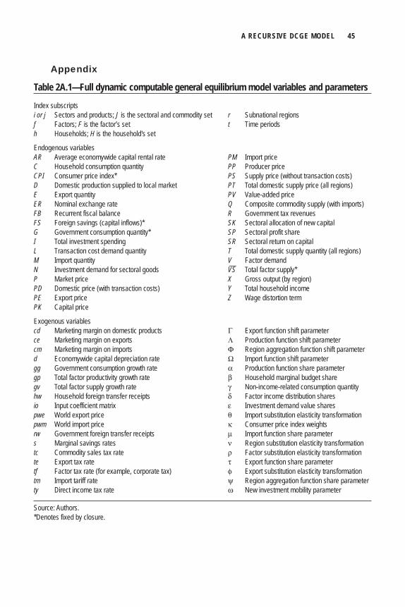
A RECURSIVE DCGE MODEL 45
Table 2A.1—Full dynamic computable general equilibrium model variables and parameters
Index subscriptsi or j Sectors and products; J is the sectoral and commodity set r Subnational regions f Factors; F is the factor’s set t Time periodsh Households; H is the household's set
Endogenous variablesAR Average economywide capital rental rate PM Import priceC Household consumption quantity PP Producer priceCPI Consumer price index* PS Supply price (without transaction costs)D Domestic production supplied to local market PT Total domestic supply price (all regions)E Export quantity PV Value-added priceER Nominal exchange rate Q Composite commodity supply (with imports)FB Recurrent fiscal balance R Government tax revenuesFS Foreign savings (capital inflows)* SK Sectoral allocation of new capitalG Government consumption quantity* SP Sectoral profit shareI Total investment spending SR Sectoral return on capitalL Transaction cost demand quantity T Total domestic supply quantity (all regions)M Import quantity V Factor demandN Investment demand for sectoral goods VS— Total factor supply*P Market price X Gross output (by region)PD Domestic price (with transaction costs) Y Total household incomePE Export price Z Wage distortion termPK Capital price
Exogenous variablescd Marketing margin on domestic products Γ Export function shift parameterce Marketing margin on exports Λ Production function shift parametercm Marketing margin on imports Φ Region aggregation function shift parameterd Economywide capital depreciation rate Ω Import function shift parametergg Government consumption growth rate α Production function share parametergp Total factor productivity growth rate β Household marginal budget sharegv Total factor supply growth rate γ Non-income-related consumption quantityhw Household foreign transfer receipts δ Factor income distribution sharesio Input coefficient matrix ε Investment demand value sharespwe World export price θ Import substitution elasticity transformationpwm World import price κ Consumer price index weightsrw Government foreign transfer receipts μ Import function share parameters Marginal savings rates ν Region substitution elasticity transformationtc Commodity sales tax rate ρ Factor substitution elasticity transformationte Export tax rate τ Export function share parametertf Factor tax rate (for example, corporate tax) φ Export substitution elasticity transformationtm Import tariff rate ψ Region aggregation function share parameterty Direct income tax rate ω New investment mobility parameter
Source: Authors.*Denotes fixed by closure.
Appendix
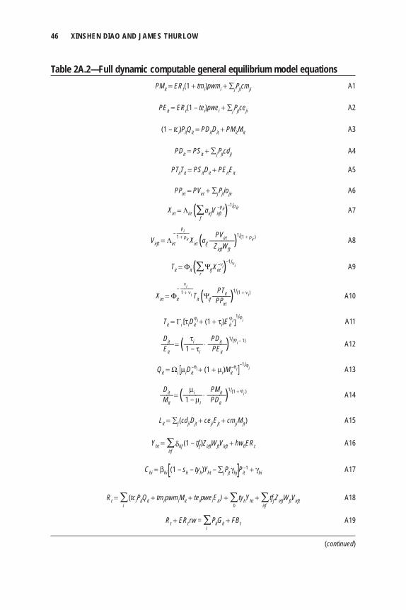
46 XINSHEN DIAO AND JAMES THURLOW
Table 2A.2—Full dynamic computable general equilibrium model equations PMit = ERt(1 + tmi)pwmi + ∑jPjtcmji A1
PEit = ERt(1 – tei)pwei + ∑jPjtceji A2
(1 – tci)PitQit = PDitDit + PMitMit A3 PDit = PSit + ∑ jPjtcdji A4
PTitTit = PSitDit + PEitEit A5 PPirt = PVirt + ∑jPjtiojir A6 Xirt = Λirt (∑airfV irft
–ρir)–1/ ρir A7 f
ρi – ——— PVirt 1 + ρir Virft = Λirt Xirt (aif ————)1/ (1 + ρir )
ZirftWft A8
Tit = Φit (∑Ψif Xirt–νi)–1/ νi A9 r
νi – ——— PTit 1 + νi Xirt = Φit Tit (Ψif ———)1/ (1 + νi) PPirt
A10
Tit = Γi [τiDit
ϕi + (1 + τi)E itϕi ]
1/ ϕi A11
Dit τi PDit —— = (——— ⋅ ———)1/ (ϕi – 1) A12 Eit 1 – τi PEit
Qit = Ωi [μiDit
–θi + (1 + μi)Mit–θi ]–1/ ϕi A13
Dit μi PMit —— = (——— ⋅ ———)1/ (1 + ϕi ) A14 Mit 1 – μi PDit
Lit = ∑j (cdjiDjt + cejiEjt + cmjiMjt) A15
Yht = ∑δhf (1 – tff)ZirftWftVirft + hwhERt A16 irf
Chi = βhi [(1 – sh – tyh)Yht – ∑jPjt γhj]Pit–1 + γhi A17
Rt = ∑ (tciPitQit + tmipwmiMit + teipweiEit ) + ∑ tyhYht + ∑ tff ZirftWftVirft A18 i h irf
Rt + ERtrw = ∑PitGit + FBt A19 i
(continued)
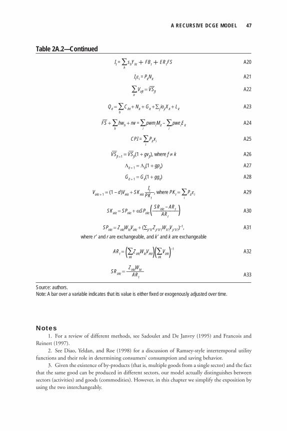
A RECURSIVE DCGE MODEL 47
Table 2A.2—Continued
It = ∑shYht + FBt + ERtFS A20 h
Itεi = PitNit A21
∑Virft = VS—ft A22 ir
Qit = ∑Ciht + Nit + Git +∑ j ioji Xit + Lit A23 h
FS— + ∑hwh + rw = ∑pwmiMit – ∑pweiEit A24 h i i
CPI = ∑Pitxi A25 i
VS—ft +1 = VS—
ft(1 + gvft), where f ≠ k A26
Λit + 1 = Λit(1 + gpit) A27
Git + 1 = Git(1 + ggit) A28
It Virkt + 1 = (1 – d)Virkt + SKirkt —— , where PKt = ∑Pitεi A29 PKt i
SRirkt – ARt SKirkt = SPirkt + ωSPirkt (——————) A30 ARt
SPirkt = ZirktWktVirkt + (∑jr ′k′Zjr ′k′tWk′tVjr ′k′t)–1, A31
where r′ and r are exchangeable, and k′ and k are exchangeable
ARt = (∑ZirktWktVirkt)(∑Virkt)–1 A32 irk irk
ZirktWkt SRirkt = ———— ARt A33
Source: authors.Note: A bar over a variable indicates that its value is either fixed or exogenously adjusted over time.
Notes 1. For a review of different methods, see Sadoulet and De Janvry (1995) and Francois and Reinert (1997). 2. See Diao, Yeldan, and Roe (1998) for a discussion of Ramsey-style intertemporal utility functions and their role in determining consumers’ consumption and saving behavior. 3. Given the existence of by-products (that is, multiple goods from a single sector) and the fact that the same good can be produced in different sectors, our model actually distinguishes between sectors (activities) and goods (commodities). However, in this chapter we simplify the exposition by using the two interchangeably.
48 XINSHEN DIAO AND JAMES THURLOW
4. In reality, part of factor incomes (for example, the return to capital) can be owned by the government or foreign institutions. Although this situation is allowed in the model that we actually implement in each case study, at this stage we ignore nonhousehold factor ownership to simplify the discussion. 5. Note that our third closure rule made G exogenous in Equation 15. 6. Lofgren, Harris, and Robinson (2001) developed an earlier version of the static component of our CGE model. 7. For mobile factors, Z and VS remain constant, and W and V adjust to clear factor markets. For sector-specifi c factors, such as capital, W and V are fi xed, and Z and VS are the adjustment variables. 8. The equations defi ning SP, SR, and AR are shown in Table 2A.2 in the appendix to this chapter (Equations A31–A33). 9. The full specifi cation of the model is provided in Table 2A.2 in the appendix to this chapter. 10. For detailed discussions of SAMs see, for example, Pyatt and Round (1985) and Reinert and Roland-Holst (1997). 11. Three poverty measures are commonly used in the literature and are also used in this book. The poverty headcount ratio (or “poverty rate” or “incidence” of poverty) is the proportion of the population with per capita consumption below the poverty line. The poverty gap (or “depth” of poverty) is the extent, measured as a proportion of the poverty line, to which a given group of poor people’s consumption level falls below the poverty line. The squared poverty gap (or “severity” of poverty) is the average of the squared values of the poverty gaps for different groups of poor people (see Foster, Greer, and Thorbecke, 1984, for details). 12. For income-based microsimulation modules with occupational choice, see Cogneau, Grimm, and Robilliard (2003) and Cogneau and Robilliard (2007).
ReferencesArmington, P. A. 1969. “A Theory of Demand for Products Distinguished by Place of Production.”
IMF Staff Papers 16 (1): 159–178.
Arndt, C., and J. Thurlow. 2010. “Mozambique.” In Agricultural Price Distortions, Inequality and
Poverty, edited by K. Anderson, J. Cockburn, and W. Martin, 303–329. Washington, DC: World
Bank.
Arndt, C., S. Robinson, and F. Tarp. 2002. “Parameter Estimation for a Computable General
Equilibrium Model: A Maximum Entropy Approach.” Economic Modelling 19: 375–398.
Behar, A. 2009. Direct Technical Change, the Elasticity of Substitution and Wage Inequality in Developing
Countries. Discussion paper 467. Oxford, UK: Department of Economics, University of Oxford.
Boys, K. A., and R. J. G. M. Florax. 2008. “Meta-Regression Estimates for CGE Models: Input
Substitution Elasticities in Production Agriculture.” Paper presented at the Eleventh Annual
Conference on Global Economic Analysis, Helsinki, Finland, June 12–14.
Cogneau, D., and A. S. Robilliard. 2007. “Growth, Distribution and Poverty in Madagascar: Learning
from a Microsimulation Model in a General Equilibrium Framework.” In Microsimulation as a
A RECURSIVE DCGE MODEL 49
Tool for the Evaluation of Public Policies: Methods and Applications, edited by A. Spadaro, 73–110.
Bilbao, Spain: Fundación BBVA.
Cogneau, D., M. Grimm, and A. S. Robilliard. 2003. “Evaluating Poverty Reduction Policies: The
Contribution of Micro-Simulation Technique.” In New International Poverty Reduction Strategies,
edited by J. P. Cling, M. Razafi ndrakato, and F. Roubaud, 340–370. London: Routledge.
Deaton, A. 2005. “Measuring Poverty in a Growing World (or Measuring Growth in a Poor World).”
Review of Economics and Statistics 57 (1): 1–19.
Delgado, C., J. Hopkins, and V. A. Kelly. 1998. Agricultural Growth Linkages in Sub-Saharan Africa.
Research Report 107. Washington, DC: International Food Policy Research Institute.
Dervis, K., J. de Melo, and S. Robinson. 1982. General Equilibrium Models for Development Policy. New
York: Cambridge University Press.
Diao, X., E. Yeldan, and T. Roe. 1998. “A Simple Dynamic Applied General Equilibrium Model of
a Small Open Economy: Transitional Dynamics and Trade Policy.” Journal of Economic Development
23 (1): 77–101.
Dimaranan, B., ed. 2006. Global Trade, Assistance, and Production: The GTAP 6 Database. West
Lafayette IN, US: Center for Global Trade Analysis, Purdue University.
Fields, G. S. 2009. “Segmented Labor Market Models in Developing Countries.” In The Oxford
Handbook of Philosophy of Economics, edited by H. Kincaid and D. Ross, 476–510. Oxford, UK:
Oxford University Press.
Foster, J., J. Greer, and E. Thorbecke. 1984. “A Class of Decomposable Poverty Measures.” Econometrica
52 (3): 761–766.
Francois, J. F., and K. A. Reinert, eds. 1997. Applied Methods for Trade Policy Analysis: A Handbook. New
York: Cambridge University Press.
Frisch, R. 1959. “A Complete Scheme for Computing All Direct and Cross Demand Elasticities in a
Model with Many Sectors.” Econometrica 27 (2): 177–196.
Haggblade, S., J. Hammer, and P. B. R. Hazell. 1991. “Modeling Agricultural Growth Multipliers.”
American Journal of Agricultural Economics 73 (2): 361–374.
Hertel, T. W. 1997. Global Trade Analysis: Modeling and Applications. Cambridge, UK: Cambridge
University Press.
King, R. P., and D. Byerlee. 1978. “Factor Intensities and Locational Linkages of Rural Consumption
Patterns in Sierra Leone.” American Journal of Agricultural Economics 60 (2): 197–206.
Lofgren, H., and S. Robinson. 1999. “Nonseparable Farm Household Decisions in a Computable
General Equilibrium Model.” American Journal of Agricultural Economics 81 (3): 663–670.
Lofgren, H., R. Harris, and S. Robinson. 2001. A Standard Computable General Equilibrium (CGE)
Model in GAMS. Microcomputers in Policy Research 5. Washington, DC: International Food
Policy Research Institute.
50 XINSHEN DIAO AND JAMES THURLOW
Pyatt, G., and J. I. Round. 1985. Social Accounting Matrices: A Basis for Planning. Washington, DC:
World Bank.
Ravallion, M. 2003. “Measuring Aggregate Welfare in Developing Countries: How Well Do National
Accounts and Surveys Agree?” Review of Economics and Statistics 85 (3): 645–652.
Reinert, K. A., and D. W. Roland-Holst. 1997. “Social Accounting Matrices.” In Applied Methods for
Trade Policy Analysis: A Handbook, edited by J. F. Francois and K. A. Reinert. New York: Cambridge
University Press.
Robinson, S., A. Cattaneo, and M. El-Said. 2001. “Updating and Estimating a Social Accounting
Matrix Using Cross Entropy Methods.” Economic Systems Research 13 (1): 47–64.
Rosegrant, M. W., C. Ringler, S. Msangi, T. B. Sulser, T. Zhu, and S. A. Cline. 2008. International
Model for Policy Analysis of Agricultural Commodities and Trade (IMPACT): Model Description.
Washington, DC: International Food Policy Research Institute.
Sadoulet, E., and A. De Janvry. 1995. Quantitative Development Policy Analysis. Baltimore: Johns
Hopkins University Press.
Sala-i-Martin, X., and M. Pinkovskiy. 2010. African Poverty Is Falling . . . Much Faster than You Think!.
Working Paper 15775. Cambridge, MA, US: National Bureau of Economic Research.
UNU, WHO, and FAO (United Nations University, World Health Organization, and Food and
Agriculture Organization of the United Nations). 2004. Human Energy Requirements: Report of a
Joint FAO/WHO/UNU Expert Consultation, Rome, October 17–24, 2001. Food and Nutrition
Technical Report Series 1. Rome.
C h a p t e r 3
Estimating Public Agricultural Expenditure Requirements
Samuel Benin, Shenggen Fan, and Michael Johnson
This chapter outlines an approach to estimating the public agricultural financial resources needed to bring about a certain rate of agricultural growth. Studies that estimate the public financial resources required to achieve specific
development objectives have focused on costing the Millennium Development Goals (MDGs). Public agricultural financial resources needed to achieve specific agricultural development objectives or broader targets are dealt with indirectly in a few studies only. The most common approach for estimating required pub-lic resources is the unit-cost method (UNDP 2003; Kenya, MPND 2005; Fan and Rosegrant 2008), where the amount of input (for example, x tons of fertil-izer or number of extension agents) required to achieve a specific objective (for example, y percent of crop area under fertilizer or extension–farmer ratio) is first calculated. Then the amount of public financial resources required to achieve the objective is estimated by multiplying the total amount of input required by the unit cost of the input. In principle, the unit cost of the input should include any related operational, administrative, or overhead cost required to manage and deliver the input. The resulting estimate can be projected into the future depend-ing on the desired outcome and the expected unit cost of the relevant inputs needed to achieve the outcome. The main drawback with using the unit-cost approach is the lack of a consistent analytical basis. There is no one-to-one rela-tionship between expenditures (or inputs) and outcomes (for example, agricul-tural growth or poverty), and so estimating the unit cost of achieving a particular outcome (for example, y percent agricultural growth rate or poverty rate) is
52 SAMUEL BENIN, SHENGGEN FAN, AND MICHAEL JOHNSON
illusive. Realization of outcomes depends on several other factors, some of which may enhance or reduce the effects of the expenditures.
From the policy perspective of using public spending for stimulating growth and reducing poverty, methods based on expenditure–growth, expenditure–poverty, and growth–poverty elasticities are conceptually sound.1 Again, existing studies that have used this type of approach have focused on costing of the MDGs (for example, Kakwani and Son 2006; Fan and Rosegrant 2008). Comparison of the results from the different studies reveals a large divergence in the estimated resources required to achieve the MDGs,2 which highlights the inconsistencies across the methods and analytical approaches used, including underlying assumptions of initial conditions and patterns of growth as well as data on elasticities and other related parameters.
The studies, nevertheless, raise some important issues that we consider in developing the approach presented in this study. An important issue is potential crowding out of private investment by public spending. This issue derives from the relative effi ciency of public versus private investments, especially where public and private spending is considered a zero-sum game, in the sense that government spending is fi nanced by taxation of private investment. Kakwani and Son (2006), for example, argue that when productivity of private investment is greater than that of public investment, as shown is some studies (for example, Ashipala and Haimbodi 2003), crowding-out effects of public investment result in a loss of growth, and, therefore, a greater amount of public resources will be required to achieve a specifi c growth objective. In contrast, crowding-out effects of public investment on private investment can lead to greater growth if public investment is more productive than private investment.
It is also important to consider the relative effects of different types of public investment in a particular sector, because public investment is not growth neutral among subsectors. The work by Fan and others (for example, Fan 2008; Mogues, Ayele, and Paulos 2008) shows that different types of public investment, both across and within sectors, affect growth and poverty differently through different path-ways and at different levels (Benin et al. 2008a). Another key factor to consider in the estimation is the initial conditions of development and patterns of growth (Kakwani and Son 2006). We fi rst conceptualize the changes in public spending as a source of agricultural growth and then develop a simple method to estimate the amount of total agricultural expenditure required to achieve certain agricultural growth rates simulated in the dynamic computable general equilibrium (DCGE) model. Because public spending on the nonagricultural sector also contributes to agricultural growth, both directly and indirectly through interactions with public agricultural expenditure (PAE), changes in public spending on the nonagricultural sector are considered in the estimation.
ESTIMATING PUBLIC SPENDING REQUIREMENTS 53
Sources of Agricultural Growth and the Contribution of Public SpendingLet aggregate agricultural output Qt in time t be represented by the following simpli-fi ed production function:
Qt = ηi f (Ft ), (1)
where Ft is the vector of factors used in the production process. There are two sources of agricultural growth: the fi rst derives from accumulation of the factors of produc-tion and their productivity; the second, which is measured by η, derives from changes in total agricultural output that cannot be explained by changes in the fac-tors of production and their productivities. This second part is referred to as total factor productivity (TFP) or what is commonly known as the Solow residual (see Romer 2000). To explain these two sources of growth further, consider a Cobb–Douglas production function of the following form:
Qt = ηi ∏Fi,tαi, (2)
i
where Fi denotes the ith factor, such as land, labor, capital; and αi measures the productivity of the ith factor.3 Differentiating Qt with respect to t gives the change in agricultural output Qt:
4
∂Qt ∂Qt Qt = —— ηt + ∑ —— Fit . (3) ∂ηt i ∂Fit
Using the results ∂Q/∂η = Q/η and ∂Q/∂Fi = αiQ/Fi (obtained from the production function) in Equation 3 and then dividing through the resulting expression by Qt, we obtain the following expression for the agricultural growth rate:
Qt ηt Fit —— = — + ∑αi —, (4) Qt ηt i Fit
where the fi rst term on the right-hand side measures the source of agricultural growth deriving from growth in TFP; the other terms together measure the source of growth deriving from accumulation of the factors of production and their respec-tive productivities αi. To determine the sources of agricultural growth deriving from growth in public spending, we need to fi rst understand what determines growth in TFP (ηt) and factor accumulation (Ft).
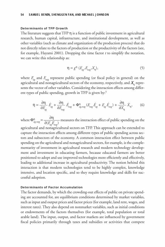
54 SAMUEL BENIN, SHENGGEN FAN, AND MICHAEL JOHNSON
Determinants of TFP GrowthThe literature suggests that TFP η is a function of public investment in agricultural research, human capital, infrastructure, and institutional development, as well as other variables (such as climate and organization of the production process) that do not directly relate to the factors of production or the productivity of the factors (see, for example, Hayami 2001). Dropping the time factor t to simplify the notation, we can write this relationship as:
η = gη (Eag ,Enag ,Xη), (5)
where Eag and Enag represent public spending (or fi scal policy in general) on the agricultural and nonagricultural sectors of the economy, respectively, and Xη repre-sents the vector of other variables. Considering the interaction effects among differ-ent types of public spending, growth in TFP is given by:5
∂η ∂η ∂η η = —— Eag + —— Enag + Φη
ag,nag (Enag Eag + Eag Enag ) + —— Xη, (6) ∂Eag ∂Enag ∂Xη
∂ηwhere Φη
ag,nag = ———— measures the interaction effect of public spending on the ∂(EagEnag)agricultural and nonagricultural sectors on TFP. This approach can be extended to capture the interaction effects among different types of public spending across sec-tors and subsectors of the economy. A common interaction effect between public spending on the agricultural and nonagricultural sectors, for example, is the comple-mentarity of investment in agricultural research and modern technology develop-ment and investment in educating farmers, because educated farmers are better positioned to adopt and use improved technologies more effi ciently and effectively, leading to additional increase in agricultural productivity. The notion behind this interaction is that modern technologies tend to be highly complex, knowledge intensive, and location specifi c, and so they require knowledge and skills for suc-cessful adoption.
Determinants of Factor AccumulationThe factor demands, by which the crowding-out effects of public on private spend-ing are accounted for, are equilibrium conditions determined by market variables, such as input and output prices and factor prices (for example, land rent, wages, and interest rates). They also depend on nonmarket variables, such as initial conditions or endowments of the factors themselves (for example, total population or total arable land). The input, output, and factor markets are infl uenced by government fi scal policies primarily through taxes and subsidies or activities that compete
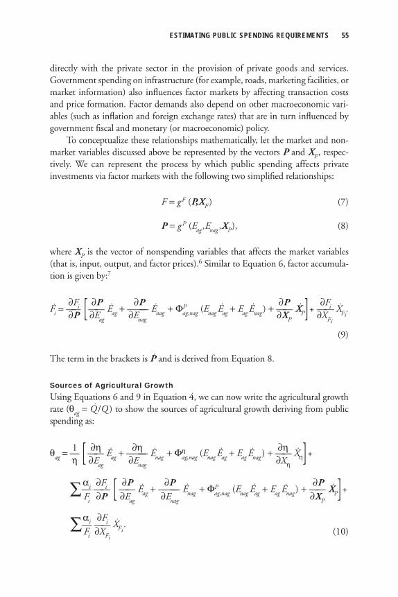
ESTIMATING PUBLIC SPENDING REQUIREMENTS 55
directly with the private sector in the provision of private goods and services. Government spending on infrastructure (for example, roads, marketing facilities, or market information) also infl uences factor markets by affecting transaction costs and price formation. Factor demands also depend on other macroeconomic vari-ables (such as infl ation and foreign exchange rates) that are in turn infl uenced by government fi scal and monetary (or macroeconomic) policy.
To conceptualize these relationships mathematically, let the market and non-market variables discussed above be represented by the vectors P and XF, respec-tively. We can represent the process by which public spending affects private investments via factor markets with the following two simplifi ed relationships:
F = g F (P,XF ) (7)
P = g P (Eag ,Enag ,XP), (8)
where XP is the vector of nonspending variables that affects the market variables (that is, input, output, and factor prices).6 Similar to Equation 6, factor accumula-tion is given by:7
∂Fi ∂P ∂P ∂P ∂Fi Fi = —— [ —— Eag + ——— Enag + ΦPag,nag (Enag Eag + Eag Enag ) + —— XP]+ —— XFi
. ∂P ∂Eag ∂Enag ∂XP ∂XFi
(9)
The term in the brackets is P and is derived from Equation 8.
Sources of Agricultural GrowthUsing Equations 6 and 9 in Equation 4, we can now write the agricultural growth rate (θag = Q /Q ) to show the sources of agricultural growth deriving from public spending as:
1 ∂η ∂η ∂ηθag = — [ —— Eag + ——— Enag + Φηag,nag (Enag Eag + Eag Enag ) + —— Xη]+
η ∂Eag ∂Enag ∂Xη
αi ∂Fi ∂P ∂P ∂P∑— —— [ —— Eag + ——— Enag + ΦPag,nag (Enag Eag + Eag Enag ) + —— XP]+
Fi ∂P ∂Eag ∂Enag ∂XP
αi ∂Fi∑— —— XFi.
Fi ∂XFi (10)
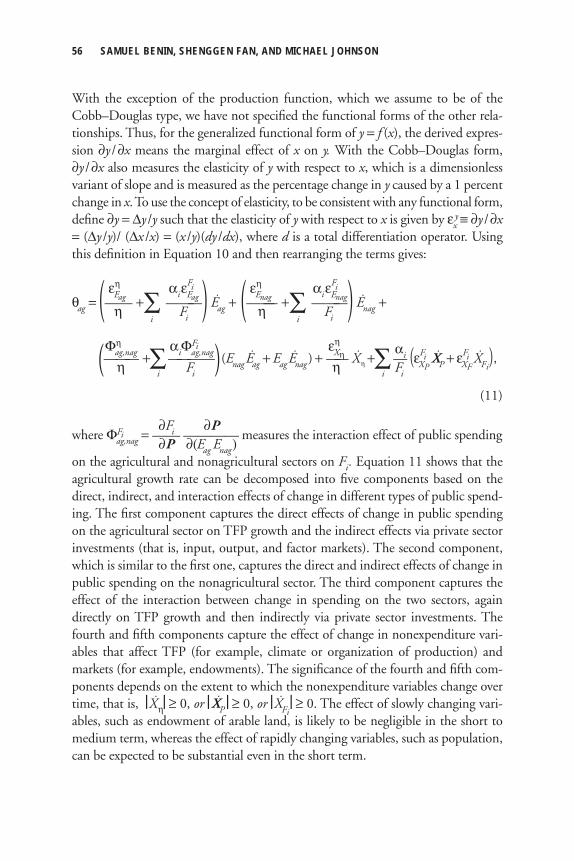
56 SAMUEL BENIN, SHENGGEN FAN, AND MICHAEL JOHNSON
With the exception of the production function, which we assume to be of the Cobb–Douglas type, we have not specifi ed the functional forms of the other rela-tionships. Thus, for the generalized functional form of y = f (x), the derived expres-sion ∂y / ∂x means the marginal effect of x on y. With the Cobb–Douglas form, ∂y / ∂x also measures the elasticity of y with respect to x, which is a dimensionless variant of slope and is measured as the percentage change in y caused by a 1 percent change in x. To use the concept of elasticity, to be consistent with any functional form, defi ne ∂y = Δy /y such that the elasticity of y with respect to x is given by ε y
x ≡ ∂y / ∂x = (Δy /y)/ (Δx /x) = (x /y)(dy /dx), where d is a total differentiation operator. Using this defi nition in Equation 10 and then rearranging the terms gives:
εηEag
αi εFi
Eag εη
Enag αi
εFiEnagθag = (—— +∑ ———) Eag + (——— +∑ ———) Enag + η
i Fi η
i Fi
Φηag,nag αiΦ
Fiag,nag εη
Xη αi(——— +∑ — ———) (Enag Eag + Eag Enag ) + —— Xη +∑
— (εFiXP
XP + εFiXF
XFi),
η i Fi η i Fi
(11)
∂Fi ∂Pwhere ΦFi
ag,nag = —— ———— measures the interaction effect of public spending ∂P ∂(Eag Enag)on the agricultural and nonagricultural sectors on Fi. Equation 11 shows that the agricultural growth rate can be decomposed into fi ve components based on the direct, indirect, and interaction effects of change in different types of public spend-ing. The fi rst component captures the direct effects of change in public spending on the agricultural sector on TFP growth and the indirect effects via private sector investments (that is, input, output, and factor markets). The second component, which is similar to the fi rst one, captures the direct and indirect effects of change in public spending on the nonagricultural sector. The third component captures the effect of the interaction between change in spending on the two sectors, again directly on TFP growth and then indirectly via private sector investments. The fourth and fi fth components capture the effect of change in nonexpenditure vari-ables that affect TFP (for example, climate or organization of production) and markets (for example, endowments). The signifi cance of the fourth and fi fth com-ponents depends on the extent to which the nonexpenditure variables change over time, that is, ⎜Xη⎜≥ 0, or ⎜XP ⎜≥ 0, or ⎜XFi
⎜≥ 0. The effect of slowly changing vari-ables, such as endowment of arable land, is likely to be negligible in the short to medium term, whereas the effect of rapidly changing variables, such as population, can be expected to be substantial even in the short term.
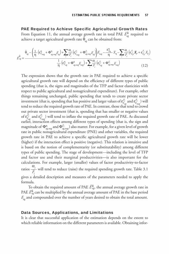
ESTIMATING PUBLIC SPENDING REQUIREMENTS 57
PAE Required to Achieve Specific Agricultural Growth RatesFrom Equation 11, the annual average growth rate in total PAE E θ
ag required to achieve a target agricultural growth rate θag can be obtained from:
(12)
The expression shows that the growth rate in PAE required to achieve a specifi c agricultural growth rate will depend on the effi ciency of different types of public spending (that is, the signs and magnitudes of the TFP and factor elasticities with respect to public agricultural and nonagricultural expenditure). For example, other things remaining unchanged, public spending that tends to create private sector investment (that is, spending that has positive and larger values of εFi
Eag and εFiEnag
) will tend to reduce the required growth rate of PAE. In contrast, those that tend to crowd out private sector investment (that is, spending that has smaller or negative values of εFi
Eag and εFi
Enag) will tend to infl ate the required growth rate of PAE. As discussed
earlier, interaction effects among different types of spending (that is, the sign and magnitude of Φη
ag,nag and ΦFiag,nag ) also matter. For example, for a given level of growth
rate in public nonagricultural expenditure (PNE) and other variables, the required growth rate in PAE to achieve a specifi c agricultural growth rate will be lower (higher) if the interaction effect is positive (negative). This relation is intuitive and is based on the notion of complementarity (or substitutability) among different types of public spending. The stage of development—including the level of TFP and factor use and their marginal productivities—is also important for the calculations. For example, larger (smaller) values of factor productivity-to-factor αiratios —— will tend to reduce (raise) the required spending growth rate. Table 3.1 Figives a detailed description and measures of the parameters needed to apply the formula.
To obtain the required amount of PAE E θag, the annual average growth rate in
PAE E θag can be multiplied by the annual average amount of PAE in the base period
Eag and compounded over the number of years desired to obtain the total amount.
Data Sources, Applications, and LimitationsIt is clear that successful application of the estimation depends on the extent to which reliable information on the different parameters is available. Obtaining infor-
˘
1 αi εη
Xη αi θag – (— (εη
Enag + Φηag,nagEag) + ∑— (εFi
Enag + Φ
Fiag,nag Eag))Enag – —— Xη –∑— (εFi
XPXP + εFi
XF XFi
) η i Fi η
i Fi
Eθag = ———————————————————————————————————— .
1 αi — (εηEag + Φη
ag,nagEnag) + ∑— (εFiEag
+ ΦFiag,nag Enag) η
i Fi
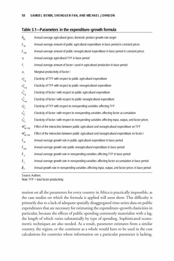
58 SAMUEL BENIN, SHENGGEN FAN, AND MICHAEL JOHNSON
mation on all the parameters for every country in Africa is practically impossible, as the case studies on which the formula is applied will soon show. This diffi culty is primarily due to a lack of adequate spatially disaggregated time-series data on public expenditures that are necessary for estimating the expenditure–growth elasticities in particular, because the effects of public spending commonly materialize with a lag, the length of which varies substantially by type of spending. Sophisticated econo-metric techniques are also needed. As a result, parameter estimates from a similar country, the region, or the continent as a whole would have to be used in the cost calculations for countries where information on a particular parameter is lacking.
Table 3.1—Parameters in the expenditure–growth formula
θag Annual average agricultural gross domestic product growth-rate target
Eag Annual average amount of public agricultural expenditure in base period in constant prices
Enag Annual average amount of public nonagricultural expenditure in base period in constant prices
η Annual average agricultural TFP in base period
Fi Annual average amount of factor i used in agricultural production in base period
αi Marginal productivity of factor i
εηEag
Elasticity of TFP with respect to public agricultural expenditure
εηEnag
Elasticity of TFP with respect to public nonagricultural expenditure
εFiEag
Elasticity of factor i with respect to public agricultural expenditure
εFiEnag
Elasticity of factor i with respect to public nonagricultural expenditure
εηXη
Elasticity of TFP with respect to nonspending variables affecting TFP
εFiXF
Elasticity of factor i with respect to nonspending variables affecting factor accumulation
εFiXP
Elasticity of factor i with respect to nonspending variables affecting input, output, and factor prices
Φηag, nag Effect of the interaction between public agricultural and nonagricultural expenditure on TFP
ΦFiag, nag Effect of the interaction between public agricultural and nonagricultural expenditure on factor i
E·ag Annual average growth rate in public agricultural expenditure in base period
E·nag Annual average growth rate public nonagricultural expenditure in base period
X· η Annual average growth rate in nonspending variables affecting TFP in base period
X· Fi Annual average growth rate in nonspending variables affecting factor accumulation in base period
X· P Annual growth rate in nonspending variables affecting input, output, and factor prices in base period
Source: Authors.Note: TFP = total factor productivity.
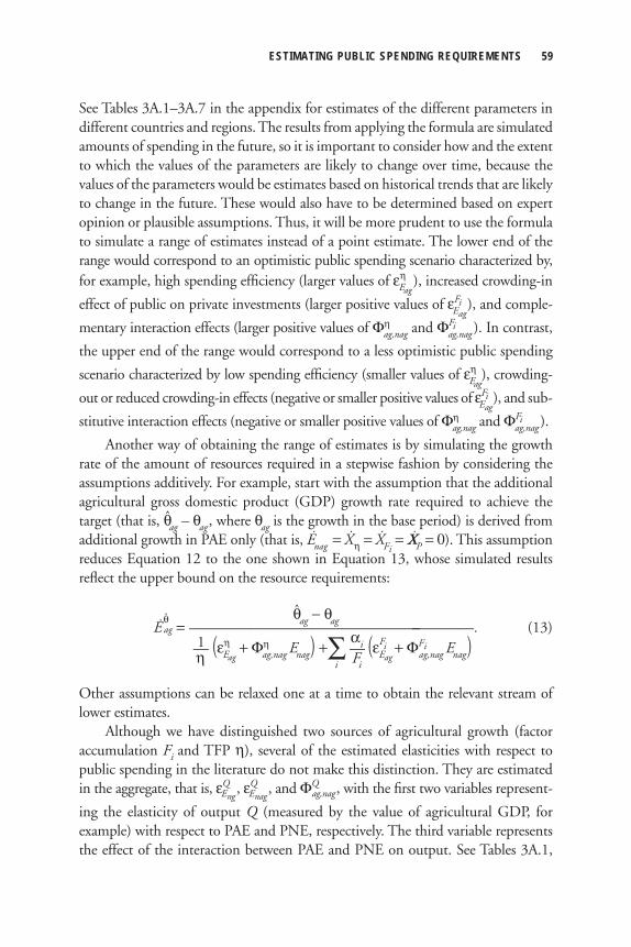
ESTIMATING PUBLIC SPENDING REQUIREMENTS 59
See Tables 3A.1–3A.7 in the appendix for estimates of the different parameters in different countries and regions. The results from applying the formula are simulated amounts of spending in the future, so it is important to consider how and the extent to which the values of the parameters are likely to change over time, because the values of the parameters would be estimates based on historical trends that are likely to change in the future. These would also have to be determined based on expert opinion or plausible assumptions. Thus, it will be more prudent to use the formula to simulate a range of estimates instead of a point estimate. The lower end of the range would correspond to an optimistic public spending scenario characterized by,for example, high spending effi ciency (larger values of εη
Eag), increased crowding-in
effect of public on private investments (larger positive values of εFiEag
), and comple-
mentary interaction effects (larger positive values of Φηag,nag and ΦFi
ag,nag ). In contrast,
the upper end of the range would correspond to a less optimistic public spending
scenario characterized by low spending effi ciency (smaller values of εηEag
), crowding-
out or reduced crowding-in effects (negative or smaller positive values of εFiEag
), and sub-
stitutive interaction effects (negative or smaller positive values of Φηag,nag and ΦFi
ag,nag ).
Another way of obtaining the range of estimates is by simulating the growth rate of the amount of resources required in a stepwise fashion by considering the assumptions additively. For example, start with the assumption that the additional agricultural gross domestic product (GDP) growth rate required to achieve the target (that is, θag – θag, where θag is the growth in the base period) is derived from additional growth in PAE only (that is, Enag = Xη = XFi
= XP = 0). This assumption reduces Equation 12 to the one shown in Equation 13, whose simulated results refl ect the upper bound on the resource requirements:
θag − θag Eθag = ———————————————————. (13)
1 αi— (εηEag + Φη
ag,nag Enag) +∑ — (εFi
Eag + ΦFi
ag,nag Enag) η i Fi
Other assumptions can be relaxed one at a time to obtain the relevant stream of lower estimates.
Although we have distinguished two sources of agricultural growth (factor accumulation Fi and TFP η), several of the estimated elasticities with respect to public spending in the literature do not make this distinction. They are estimatedin the aggregate, that is, εQ
Eng, εQ
Enag, and ΦQ
ag,nag, with the fi rst two variables represent-
ing the elasticity of output Q (measured by the value of agricultural GDP, for example) with respect to PAE and PNE, respectively. The third variable represents the effect of the interaction between PAE and PNE on output. See Tables 3A.1,
60 SAMUEL BENIN, SHENGGEN FAN, AND MICHAEL JOHNSON
3A.2, and 3A.5 for measures of these variables. This aggregation simplifi es the appli-cation of Equation 13 further and is, in fact, how the formula is usually applied in the case studies (specifi cally, those for Ghana, Kenya, Malawi, Nigeria, Rwanda, Uganda, and Zambia). Details of exactly how aggregation is done as well as the parameters and sources of data used are discussed in the specifi c cases. We summarize the key similarities and differences here, however. The analyses for Ghana, Malawi, Nigeria, Uganda, and Zambia are most similar in terms of applying the formula as it has been presented. It was applied using simple spreadsheet analysis. The main differences are the sources of information on expenditure–growth elasticities. In the cases of Ghana and Uganda, we draw on elasticities from previous work carried out by others in the respective countries. In the case of Malawi, Nigeria, and Zambia, we rely on parameters estimated at the pan-African level, also from previous work done by others using cross-country regression techniques. Although the case study on Kenya also uses parameter estimates from other studies, specifi cally those esti-mated for Uganda, the resource requirements are simulated by directly integrating the formula in the DCGE model for Kenya through a set of nested linear equations. The approach used in the case study on Rwanda is similar to the formula presented here, although in addition it used data on expenditures of specifi c agricultural sub-sectors in the scenarios (as was done to some extent in the case study on Kenya).
In applying the formula, there are some simple assumptions to be borne in mind. The main one is that the estimated elasticities are assumed to be valid outside the range of the data used in estimating them. This assumption is used to infer outcomes associated with large changes in required growth of PAE, which is due to the large gap between the observed and target agricultural GDP growth rate in most of the case studies. In reality, elasticities may change over time to refl ect increasing or decreasing returns to public spending. These dynamic effects are diffi cult to implement in the formula adapted here, and so we assume that the values of the parameters remain unchanged over the simulation period. Although this assump-tion may seem extreme and unrealistic in some cases, the results based on it have useful implications for reforming fi scal policy and public spending to raise and maintain high agricultural productivity.
Another important consideration of the results not dealt with is how the addi-tional spending will be funded and implications of different fi nancing arrangements on the outcomes, with the exception of the Kenyan case study to some extent. One possible source of fi nancing for additional spending is from domestic sources through increased taxation of or borrowing from the savings of the private sector. Raising taxes can have negative total investment effects (that is, by crowding out private investment) to the extent that public and private spending is a zero-sum game. For example, in response to higher taxes, households may adjust their savings downward to maintain their current consumption levels, leading to a reduction in
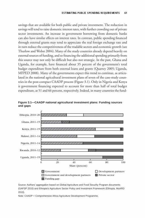
ESTIMATING PUBLIC SPENDING REQUIREMENTS 61
savings that are available for both public and private investment. The reduction in savings will tend to raise domestic interest rates, with further crowding out of private sector investments. An increase in government borrowing from domestic banks can also have similar effects on interest rates. In contrast, public spending fi nanced through external grants may tend to appreciate the real foreign exchange rate and in turn reduce the competitiveness of the tradable sectors and economic growth (see Thurlow and Wobst 2004). Many of the study countries already depend heavily on external sources of funding, and so fi nancing the additional spending primarily from this source may not only be diffi cult but also not strategic. In the past, Ghana and Uganda, for example, have fi nanced about 35 percent of the government’s total budget expenditure from both external loans and grants (Quartey 2005; Uganda, MFPED 2008). Many of the governments expect this trend to continue, as articu-lated in the national agricultural investment plans of seven of the case-study coun-tries in the post-compact CAADP process (Figure 3.1). Only in Nigeria and Kenya is government fi nancing expected to account for more than half of total budget expenditure, at 51 and 66 percent, respectively. Indeed, in many countries the fund-
Share (percent)
Uganda, 2011–15
400 20 60 80 100
Private sector
Rwanda, 2010–12
Nigeria, 2011–14
Malawi, 2011–14
Kenya, 2011–15
Ghana, 2011–15
Ethiopia, 2010–20
Development partnersGovernment
Funding gap
Government and development partners
Figure 3.1—CAADP national agricultural investment plans: Funding sources and gaps
Source: Authors’ aggregation based on Global Agriculture and Food Security Program documents (GAFSP 2010) and Ethiopia’s Agriculture Sector Policy and Investment Framework (Ethiopia, MoARD 2010).Note: CAADP = Comprehensive Africa Agriculture Development Programme.
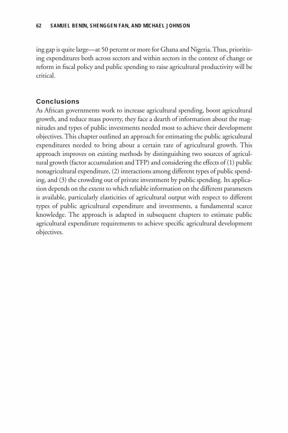
62 SAMUEL BENIN, SHENGGEN FAN, AND MICHAEL JOHNSON
ing gap is quite large—at 50 percent or more for Ghana and Nigeria. Thus, prioritiz-ing expenditures both across sectors and within sectors in the context of change or reform in fi scal policy and public spending to raise agricultural productivity will be critical.
ConclusionsAs African governments work to increase agricultural spending, boost agricultural growth, and reduce mass poverty, they face a dearth of information about the mag-nitudes and types of public investments needed most to achieve their development objectives. This chapter outlined an approach for estimating the public agricultural expenditures needed to bring about a certain rate of agricultural growth. This approach improves on existing methods by distinguishing two sources of agricul-tural growth (factor accumulation and TFP) and considering the effects of (1) public nonagricultural expenditure, (2) interactions among different types of public spend-ing, and (3) the crowding out of private investment by public spending. Its applica-tion depends on the extent to which reliable information on the different parameters is available, particularly elasticities of agricultural output with respect to different types of public agricultural expenditure and investments, a fundamental scarce knowledge. The approach is adapted in subsequent chapters to estimate public agricultural expenditure requirements to achieve specifi c agricultural development objectives.
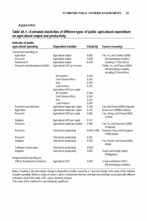
ESTIMATING PUBLIC SPENDING REQUIREMENTS 63
Table 3A.1—Estimated elasticities of different types of public agricultural expenditure on agricultural output and productivity
Indicator of public agricultural spending Dependent variable Elasticity Source (country)Government spending on: Agriculture Agricultural output 0.085 Fan, Yu, and Saurkar (2008) Research Agricultural output 0.038 (44 developing countries, Nonresearch Agricultural output –0.070 including 17 from Africa) Research and development (R&D) Agricultural GDP per hectare Thirtle, Lin, and Piesse (2003) (48 developing countries, including 22 from Africa) All countries 0.442 Sub-Saharan Africa 0.363 Asia 0.344 Latin America 0.197 Agricultural GDP per capita All countries 0.304 Sub-Saharan Africa 0.264 Asia 0.231 Latin America 0.093 Research and extension Agricultural output per capita 0.189 Fan and Zhang (2008) (Uganda) Agriculture Agricultural output per capita 0.153 Benin et al. (2008b) (Ghana) Research Agricultural GDP per capita 0.085 Fan, Zhang, and Zhang (2002) (China) Irrigation Agricultural GDP per capita 0.101 Research Agricultural output per worker 0.464 Fan, Yu, and Jitsuchon (2008) (Thailand) Research Total factor productivity 0.049–0.066 Evenson, Pray, and Rosegrant (1999) (India) Research Total factor productivity 0.255 Irrigation Total factor productivity 0.036 Fan, Hazell, and Thorat (2000) (India) Soil/water conservation Total factor productivity 0.002a Irrigation Total factor productivity 0.003 Teurel and Kuroda (2005) (Philippines)Nongovernment spending on: Official development assistance Agricultural GDP 0.030 Schuh and Norton (1991) (98 developing countries)
Notes: Elasticity is the percentage change in dependent variable caused by a 1 percent change in the value of the indicator of public spending. Where a range of values is given, it represents the low- and high-end estimates associated with different estimators used in the study. GDP = gross domestic product.aThe value of the coefficient is not statistically significant.
Appendix
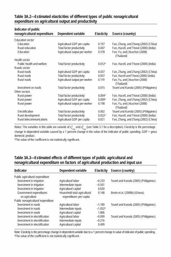
Table 3A.2—Estimated elasticities of different types of public nonagricultural expenditure on agricultural output and productivity
Indicator of public nonagricultural expenditure Dependent variable Elasticity Source (country)Education sector Education Agricultural GDP per capita 0.197 Fan, Zhang, and Zhang (2002) (China) Rural education Total factor productivity 0.047 Fan, Hazell, and Thorat (2000) (India) Education Agricultural output per worker 0.578 Fan, Yu, and Jitsuchon (2008) (Thailand)Health sector Public health and welfare Total factor productivity 0.012a Fan, Hazell, and Thorat (2000) (India)Roads sector Rural roads Agricultural GDP per capita 0.037 Fan, Zhang, and Zhang (2002) (China) Rural roads Total factor productivity 0.057 Fan, Hazell and Thorat (2000) (India) Rural roads Agricultural output per worker 0.119 Fan, Yu, and Jitsuchon (2008) (Thailand) Investment on roads Total factor productivity 0.015 Teurel and Kuroda (2005) (Philippines)Other sectors Rural power Total factor productivity 0.004a Fan, Hazell, and Thorat (2000) (India) Rural power Agricultural GDP per capita 0.009a Fan, Zhang, and Zhang (2002) (China) Rural power Agricultural output per worker 0.198 Fan, Yu, and Jitsuchon (2008) (Thailand) Electrification Total factor productivity 0.002 Teurel and Kuroda (2005) (Philippines) Rural development Total factor productivity 0.022a Fan, Hazell, and Thorat (2000) (India) Rural telecommunications Agricultural GDP per capita 0.021 Fan, Zhang, and Zhang (2002) (China)
Notes: The variables in this table are variants of εηEnag
and εQEnag
(see Table 3.1 for a description). Elasticity is the percentagechange in dependent variable caused by a 1 percent change in the value of the indicator of public spending. GDP = gross domestic product.aThe value of the coefficient is not statistically significant.
Table 3A.3—Estimated effects of different types of public agricultural and nonagricultural expenditure on factors of agricultural production and input use
Indicator Dependent variable Elasticity Source (country)Public agricultural expenditure Investment in irrigation Agricultural labor –0.233 Teurel and Kuroda (2005) (Philippines) Investment in irrigation Intermediate inputs –0.501 Investment in irrigation Agricultural capital 0.650 Government expenditures Household total agricultural 0.148 Benin et al. (2008b) (Ghana) on agriculture expenditures per capita Public nonagricultural expenditure Investment in roads Agricultural labor –1.189 Teurel and Kuroda (2005) (Philippines) Investment in roads Intermediate inputs –1.052a Investment in roads Agricultural capital 1.806 Investment in electrification Agricultural labor –0.099 Teurel and Kuroda (2005) (Philippines) Investment in electrification Intermediate inputs –0.216 Investment in electrification Agricultural capital 0.499
Note: Elasticity is the percentage change in dependent variable due to a 1 percent change in value of indicator of public spending.aThe value of the coefficient is not statistically significant.
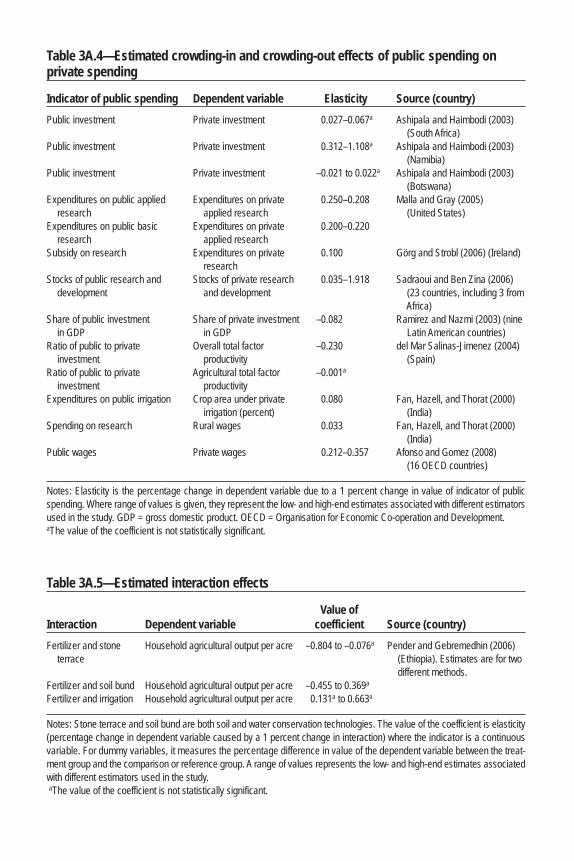
Table 3A.4—Estimated crowding-in and crowding-out effects of public spending on private spending
Indicator of public spending Dependent variable Elasticity Source (country)Public investment Private investment 0.027–0.067a Ashipala and Haimbodi (2003) (South Africa)Public investment Private investment 0.312–1.108a Ashipala and Haimbodi (2003) (Namibia)Public investment Private investment –0.021 to 0.022a Ashipala and Haimbodi (2003) (Botswana)Expenditures on public applied Expenditures on private 0.250–0.208 Malla and Gray (2005) research applied research (United States)Expenditures on public basic Expenditures on private 0.200–0.220 research applied research Subsidy on research Expenditures on private 0.100 Görg and Strobl (2006) (Ireland) research Stocks of public research and Stocks of private research 0.035–1.918 Sadraoui and Ben Zina (2006) development and development (23 countries, including 3 from Africa)Share of public investment Share of private investment –0.082 Ramirez and Nazmi (2003) (nine in GDP in GDP Latin American countries)Ratio of public to private Overall total factor –0.230 del Mar Salinas-Jimenez (2004) investment productivity (Spain)Ratio of public to private Agricultural total factor –0.001a
investment productivity Expenditures on public irrigation Crop area under private 0.080 Fan, Hazell, and Thorat (2000) irrigation (percent) (India)Spending on research Rural wages 0.033 Fan, Hazell, and Thorat (2000) (India)Public wages Private wages 0.212–0.357 Afonso and Gomez (2008) (16 OECD countries)
Notes: Elasticity is the percentage change in dependent variable due to a 1 percent change in value of indicator of public spending. Where range of values is given, they represent the low- and high-end estimates associated with different estimators used in the study. GDP = gross domestic product. OECD = Organisation for Economic Co-operation and Development.aThe value of the coefficient is not statistically significant.
Table 3A.5—Estimated interaction effects
Value ofInteraction Dependent variable coefficient Source (country)Fertilizer and stone Household agricultural output per acre –0.804 to –0.076a Pender and Gebremedhin (2006) terrace (Ethiopia). Estimates are for two different methods.Fertilizer and soil bund Household agricultural output per acre –0.455 to 0.369a
Fertilizer and irrigation Household agricultural output per acre 0.131a to 0.663a
Notes: Stone terrace and soil bund are both soil and water conservation technologies. The value of the coefficient is elasticity (percentage change in dependent variable caused by a 1 percent change in interaction) where the indicator is a continuous variable. For dummy variables, it measures the percentage difference in value of the dependent variable between the treat-ment group and the comparison or reference group. A range of values represents the low- and high-end estimates associated with different estimators used in the study. aThe value of the coefficient is not statistically significant.
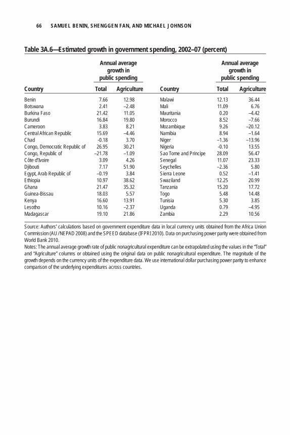
66 SAMUEL BENIN, SHENGGEN FAN, AND MICHAEL JOHNSON
Table 3A.6—Estimated growth in government spending, 2002–07 (percent)
Annual average Annual average growth in growth in public spending public spending
Country Total Agriculture Country Total AgricultureBenin 7.66 12.98 Malawi 12.13 36.44Botswana 2.41 –2.48 Mali 11.09 6.76Burkina Faso 21.42 11.05 Mauritania 0.20 –4.42Burundi 16.84 19.80 Morocco 8.52 –7.66Cameroon 3.83 8.21 Mozambique 9.26 –20.12Central African Republic 15.69 –4.46 Namibia 8.94 –1.64Chad -0.18 3.70 Niger –1.36 –13.96Congo, Democratic Republic of 26.95 30.21 Nigeria -0.10 13.55Congo, Republic of –21.78 –1.09 Sao Tome and Principe 28.09 56.47Côte d’Ivoire 3.09 4.26 Senegal 11.07 23.33Djibouti 7.17 51.90 Seychelles –2.36 5.80Egypt, Arab Republic of –0.19 3.84 Sierra Leone 0.52 –1.41Ethiopia 10.97 38.62 Swaziland 12.25 20.99Ghana 21.47 35.32 Tanzania 15.20 17.72Guinea-Bissau 18.03 5.57 Togo 5.48 14.48Kenya 16.60 13.91 Tunisia 5.30 3.85Lesotho 10.16 –2.37 Uganda 0.79 –4.95Madagascar 19.10 21.86 Zambia 2.29 10.56
Source: Authors’ calculations based on government expenditure data in local currency units obtained from the Africa Union Commission (AU / NEPAD 2008) and the SPEED database (IFPRI 2010). Data on purchasing power parity were obtained from World Bank 2010.Notes: The annual average growth rate of public nonagricultural expenditure can be extrapolated using the values in the “Total” and “Agriculture” columns or obtained using the original data on public nonagricultural expenditure. The magnitude of the growth depends on the currency units of the expenditure data. We use international dollar purchasing power parity to enhance comparison of the underlying expenditures across countries.
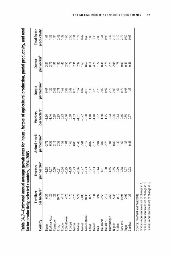
ESTIMATING PUBLIC SPENDING REQUIREMENTS 67
Tabl
e 3A.
7—Es
timat
ed an
nual
aver
age g
rowt
h ra
tes f
or in
puts
, fac
tors
of a
gricu
ltura
l pro
duct
ion,
par
tial p
rodu
ctivi
ty, an
d to
tal
fact
or p
rodu
ctivi
ty, se
lecte
d co
untri
es, 1
994–
2003
Fe
rtiliz
er
Trac
tors
An
imal
stoc
k W
orke
rs
Outp
ut
Outp
ut
Tota
l fac
tor
Coun
try
per h
ecta
rea
per h
ecta
rea
per h
ecta
rea
per h
ecta
rea
per h
ecta
reb
per w
orke
rb pr
oduc
tivity
c
Benin
6.3
7 –3
.58
–2.73
–3
.60
0.07
3.81
1.67
Burki
na F
aso
–1.26
–1
.07
0.52
–1.46
1.2
5 2.7
6 1.3
2Ca
mero
on
1.29
0.00
2.19
0.69
2.62
1.91
1.84
Chad
10
.71
–0.31
2.5
2 0.8
9 2.7
1 1.8
0 2.4
8Co
ngo
4.14
–0.54
1.5
9 0.2
3 1.6
8 1.4
5 1.3
9Cô
te d’I
voire
4.7
5 –0
.25
1.01
–0.40
2.0
9 2.5
0 1.6
0Et
hiopia
1.7
0 –1
.79
1.63
0.68
2.49
1.79
2.55
Gabo
n –2
.76
–0.73
0.0
0 –1
.53
0.75
2.31
2.31
Ghan
a 5.2
7 –3
.96
–1.48
–1
.31
1.57
2.92
1.79
Guine
a –3
.05
–0.27
2.4
1 –0
.72
0.87
1.60
0.42
Guine
a-Bi
ssau
10
.36
–2.73
–1
.17
–0.80
–0
.13
0.67
0.45
Keny
a 0.2
9 0.7
7 –0
.82
1.18
1.30
0.11
1.05
Malaw
i 7.3
4 –2
.63
–1.20
–1
.48
3.23
4.78
3.35
Mali
3.97
–0.44
2.0
4 0.5
2 2.2
5 1.7
2 2.8
5Ma
urita
nia
–2.55
1.0
1 3.8
7 1.6
0 2.0
2 0.4
1 1.4
4Ma
uritiu
s –2
.12
0.00
2.75
–1.75
0.9
7 2.7
6 0.9
3Mo
zamb
ique
4.63
–1.85
–1
.01
0.04
2.79
2.75
3.32
Nige
ria
–5.45
0.8
5 0.8
2 –0
.06
2.02
2.08
2.12
Suda
n 0.1
9 –0
.29
1.39
–0.14
1.6
4 1.7
8 3.1
9Ta
nzan
ia –1
4.94
0.38
1.69
0.66
0.74
0.09
2.79
Togo
2.9
7 –2
.27
1.33
0.55
0.96
0.41
0.59
Zamb
ia 1.2
5 –0
.03
0.46
0.77
1.23
0.46
0.03
Sour
ce: N
in Pr
att an
d Yu (
2008
).a Va
lues r
epre
sent
meas
ure o
f cha
nge i
n Fi.
b Value
s rep
rese
nt me
asur
e of c
hang
e in α
i. c Va
lues r
epre
sent
meas
ure o
f cha
nge i
n η.
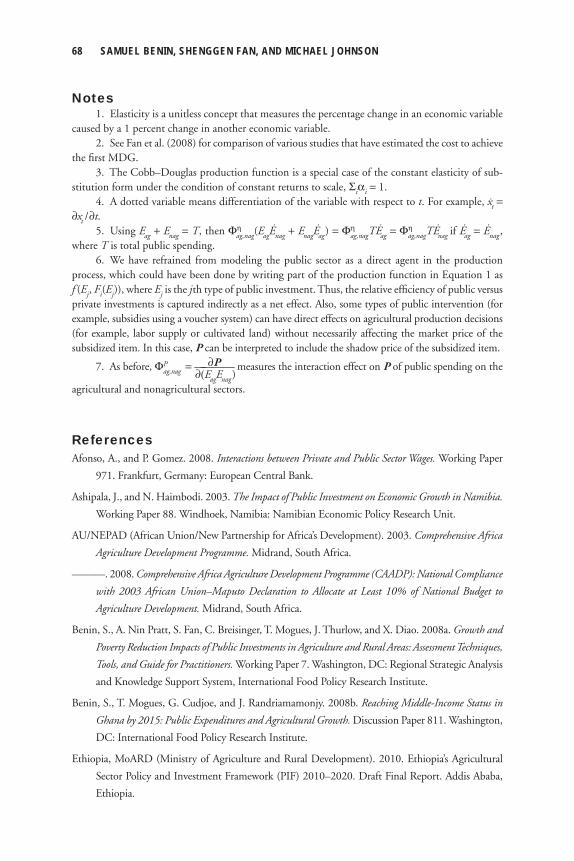
68 SAMUEL BENIN, SHENGGEN FAN, AND MICHAEL JOHNSON
Notes 1. Elasticity is a unitless concept that measures the percentage change in an economic variable caused by a 1 percent change in another economic variable. 2. See Fan et al. (2008) for comparison of various studies that have estimated the cost to achieve the fi rst MDG. 3. The Cobb–Douglas production function is a special case of the constant elasticity of sub-stitution form under the condition of constant returns to scale, Σiαi = 1. 4. A dotted variable means differentiation of the variable with respect to t. For example, xt =
∂xt / ∂t. 5. Using Eag + Enag = T, then Φη
ag,nag(EagEnag + EnagEag) = Φηag,nag
TEag = Φηag,nagTEnag if Eag = Enag,
where T is total public spending. 6. We have refrained from modeling the public sector as a direct agent in the production process, which could have been done by writing part of the production function in Equation 1 as f (Ej, Fi(Ej)), where Ej is the jth type of public investment. Thus, the relative effi ciency of public versus private investments is captured indirectly as a net effect. Also, some types of public intervention (for example, subsidies using a voucher system) can have direct effects on agricultural production decisions (for example, labor supply or cultivated land) without necessarily affecting the market price of the subsidized item. In this case, P can be interpreted to include the shadow price of the subsidized item. ∂P 7. As before, ΦP
ag,nag = ———— measures the interaction effect on P of public spending on the ∂(EagEnag)agricultural and nonagricultural sectors.
ReferencesAfonso, A., and P. Gomez. 2008. Interactions between Private and Public Sector Wages. Working Paper
971. Frankfurt, Germany: European Central Bank.
Ashipala, J., and N. Haimbodi. 2003. The Impact of Public Investment on Economic Growth in Namibia.
Working Paper 88. Windhoek, Namibia: Namibian Economic Policy Research Unit.
AU/NEPAD (African Union/New Partnership for Africa’s Development). 2003. Comprehensive Africa
Agriculture Development Programme. Midrand, South Africa.
———. 2008. Comprehensive Africa Agriculture Development Programme (CAADP): National Compliance
with 2003 African Union–Maputo Declaration to Allocate at Least 10% of National Budget to
Agriculture Development. Midrand, South Africa.
Benin, S., A. Nin Pratt, S. Fan, C. Breisinger, T. Mogues, J. Thurlow, and X. Diao. 2008a. Growth and
Poverty Reduction Impacts of Public Investments in Agriculture and Rural Areas: Assessment Techniques,
Tools, and Guide for Practitioners. Working Paper 7. Washington, DC: Regional Strategic Analysis
and Knowledge Support System, International Food Policy Research Institute.
Benin, S., T. Mogues, G. Cudjoe, and J. Randriamamonjy. 2008b. Reaching Middle-Income Status in
Ghana by 2015: Public Expenditures and Agricultural Growth. Discussion Paper 811. Washington,
DC: International Food Policy Research Institute.
Ethiopia, MoARD (Ministry of Agriculture and Rural Development). 2010. Ethiopia’s Agricultural
Sector Policy and Investment Framework (PIF) 2010–2020. Draft Final Report. Addis Ababa,
Ethiopia.
ESTIMATING PUBLIC SPENDING REQUIREMENTS 69
Evenson, R. E., C. E. Pray, and M. W. Rosegrant. 1999. Agricultural Research and Productivity Growth
in India. Research Report 109. Washington, DC: International Food Policy Research Institute.
Fan, S., ed. 2008. Public Expenditures, Growth, and Poverty: Lessons from Developing Countries. Baltimore:
Johns Hopkins University Press.
Fan, S., and M. Rosegrant. 2008. Investing in Agriculture to Overcome the World Food Crisis and Reduce
Poverty and Hunger. Policy Brief 12. Washington, DC: International Food Policy Research
Institute.
Fan, S., and X. Zhang. 2008. “Public Expenditure, Growth, and Poverty Reduction in Rural Uganda.
Development.” African Development Review 20 (3): 466–496.
Fan, S., P. Hazell, and S. Thorat. 2000. “Government Spending, Agricultural Growth and Poverty in
Rural India.” American Journal of Agricultural Economics 82 (4): 1038–1051.
Fan, S., B. Yu, and J. Jitsuchon. 2008. “Does Allocation of Public Spending Matter in Poverty
Reduction? Evidence from Thailand.” Asian Economic Journal 22 (4): 411–430.
Fan, S., B. Yu, and A. Saurkar. 2008. “Public Spending in Developing Countries: Trends, Determination,
and Impact.” In Public Expenditures, Growth, and Poverty: Lessons from Developing Countries, edited
by S. Fan, 20–55. Baltimore: Johns Hopkins University Press.
Fan, S., L. Zhang, and X. Zhang. 2002. Growth, Inequality and Poverty in Rural China: The Role of
Public Investments. Research Report 125. Washington, DC: International Food Policy Research
Institute.
Fan, S., M. Johnson, A. Saurkar, and T. Makombe. 2008. Investing in African Agriculture to Halve
Poverty by 2015. Discussion Paper 751. Washington, DC: International Food Policy Research
Institute.
GAFSP (Global Agriculture and Food Security Program). 2010. GAFSP Document Library. Accessed
December. www.gafspfund.org/gafsp/library.
Görg, H., and E. Strobl. 2006. “The Effect of R&D Subsidies on Private R&D.” Economica 74:
215–234.
Hayami, Y. 2001. Development Economics: From the Poverty to the Wealth of Nations. Oxford, UK:
Oxford University Press.
IFPRI (International Food Policy Research Institute). 2010. “Statistics on Public Expenditure for
Economic Development (SPEED)” database. Accessed January 12. www.ifpri.org/book-39/
ourwork/programs/priorities-public-investment/speed-database
Kakwani, N., and H. H. Son. 2006. How Costly Is It to Achieve the Millennium Development Goal of
Halving Poverty between 1990 and 2015? Working Paper 19. New York: International Poverty
Center, United Nations Development Program.
Kenya, MPND (Ministry of Planning and National Development). 2005. Millennium Development
Goals in Kenya: Needs and Costs. Nairobi, Kenya: Republic of Kenya.
Malla, S., and R. Gray. 2005. “The Crowding Effects of Basic and Applied Research: A Theoretical
and Empirical Analysis of an Agricultural Biotech Industry.” American Journal of Agricultural
Economics 87 (2): 423–438.
70 SAMUEL BENIN, SHENGGEN FAN, AND MICHAEL JOHNSON
del Mar Salinas-Jimenez, M. 2004. “Public Infrastructure and Private Productivity in the Spanish
Regions.” Journal of Policy Modeling 26: 47–64.
Mogues, T., G. Ayele, and Z. Paulos. 2008. The Bang for the Birr: Public Expenditures and Rural Welfare
in Ethiopia. Research Report 160. Washington, DC: International Food Policy Research Institute.
Nin Pratt, A., and B. Yu. 2008. An Updated Look at the Recovery of Agricultural Productivity in Sub-
Saharan Africa. Discussion Paper 787. Washington, DC: International Food Policy Research
Institute.
Pender, J., and B. Gebremedhin. 2006. “Land Management, Crop Production, and Household Income
in the Highlands of Tigray, Northern Ethiopia: An Econometric Analysis.” In Strategies for
Sustainable Land Management in the East African Highlands, edited by J. Pender, F. Place, and
S. Ehui, 107–139. Washington, DC: International Food Policy Research Institute.
Quartey, P. 2005. “Innovative Ways of Making Aid Effective in Ghana: Tied Aid Versus Direct
Budgetary Support.” Journal of International Development 17: 1077–1092.
Ramirez, M. D., and N. Nazmi. 2003. “Public Investment and Economic Growth in Latin America:
An Empirical Test.” Review of Development Economics 7 (1): 115–126.
Romer, D. 2000. Advanced Macroeconomics. New York: McGraw-Hill/Irwin.
Sadraoui, T., and N. Ben Zina. 2006. Complementarity and Substitutability between Public and Private
Investment in Research and Development: An Empirical Study. Working Paper 3929. Munich,
Germany: Munich Personal RePEc Archive.
Schuh, S. G., and G. W. Norton. 1991. “Agricultural Research in an International Policy Context.” In
Agricultural Research Policy: International Quantitative Perspectives, edited by P. G. Pardey,
J. Roseboom, and J. R. Anderson, 51–79. Cambridge, UK: Cambridge University Press.
Teurel, R. G., and Y. Kuroda. 2005. “Public Investment and Productivity Growth in Philippines
Agriculture, 1974–2000.” Journal of Asian Economics 6: 555–576.
Thirtle, C., L. Lin, and J. Piesse. 2003. “The Impact of Research-Led Agricultural Productivity Growth
on Poverty Reduction in Africa, Asia and Latin America.” World Development 31 (12):
1959–1975.
Thurlow, J., and P. Wobst. 2004. The Road to Pro-Poor Growth in Zambia: Past Lessons and Future
Challenges. Development Strategy and Governance Division Discussion Paper 16. Washington,
DC: International Food Policy Research Institute.
Uganda, MFPED (Ministry of Finance Planning and Economic Development). 2008. Background to
the Budget 2008/09 FY. Kampala, Uganda.
UNDP (United Nations Development Programme). 2003. Financing the Development Goals: An
Analysis of Tanzania, Cameroon, Malawi, Uganda, and The Philippines. New York.
World Bank. 2010. “World Development Indicators. 2010.” Accessed January 12. http://data
.worldbank.org/indicator/PA.NUS.PPP.
C h a p t e r 4
KenyaJames Thurlow, Jane Kiringai, and Madhur Gautam
K enya’s economy is diverse, with both agricultural and industrial potential. However, the economy has not performed especially well over the past two decades, and evidence suggests that poverty and inequality has not declined
much. Therefore, it is imperative that Kenya’s government foster stronger growth and a process of income generation that benefits the broader population. As dis-cussed in the next section, numerous studies emphasize the importance of rural development in Kenya, largely because a majority of the population, especially poor households, lives in rural areas, where they rely heavily on agricultural incomes. Urban households also depend on rural areas as a source of food and as a market for nonagricultural goods. However, Kenya’s ninth National Development Strategy has not taken a particularly optimistic view of agriculture’s potential contribution toeconomic growth—it targets an annual growth rate of around 4 percent per year, with agriculture growing at a little more than 3 percent (Kenya 2002). The strategy instead places greater emphasis on the creation of a dynamic industrial sector that provides employment opportunities and improves incomes. These objectives are important if Kenya is to diversify its economy and encourage long-term structural transformation. However, past strategies have not generated rapid economic growth,
This chapter draws on an IFPRI Discussion Paper (Thurlow, Kiringai, and Gautam 2007) to which a number of people contributed. In particular, the authors thank Bernadette Wanjala, who helped build the social accounting matrix for Kenya; James Njeru and Nicholas Waiyaki, who provided information on Kenya’s agricultural systems; and Sam Benin and Xinshen Diao, who provided technical advice during the research process. The Discussion Paper was a research output from a project funded by the World Bank.
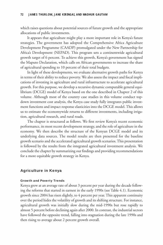
72 JAMES THURLOW, JANE KIRINGAI, AND MADHUR GAUTAM
which raises questions about potential sources of future growth and the appropriate allocations of public investments.
It appears that agriculture might play a more important role in Kenya’s future strategies. The government has adopted the Comprehensive Africa Agriculture Development Programme (CAADP) promulgated under the New Partnership for Africa’s Development (NEPAD). This program sets a continentwide agricultural growth target of 6 percent. To achieve this growth, Kenya’s government has signed the Maputo Declaration, which calls on African governments to increase the share of agricultural spending to 10 percent of their total budgets.
In light of these developments, we evaluate alternative growth paths for Kenya in terms of their ability to reduce poverty. We also assess the impact and fi scal impli-cations of investing in agriculture and rural infrastructure to accelerate agricultural growth. For this purpose, we develop a recursive dynamic computable general equi-librium (DCGE) model of Kenya based on the one described in Chapter 2 of this volume. Although most of the country case studies in this volume conduct top-down investment cost analysis, the Kenya case study fully integrates public invest-ment functions and impact response elasticities into the DCGE model. This allows us to estimate the economywide returns to different investments, including irriga-tion, agricultural research, and rural roads.
The chapter is structured as follows. We fi rst review Kenya’s recent economic performance, its most recent development strategy, and the role of agriculture in the economy. We then describe the structure of the Kenyan DCGE model and its underlying data sources. The model results are then presented for the baseline growth scenario and the accelerated agricultural growth scenarios. This presentation is followed by the results from the integrated agricultural investment analysis. We conclude the chapter by summarizing our fi ndings and providing recommendations for a more equitable growth strategy in Kenya.
Agriculture in Kenya
Growth and Poverty TrendsKenya grew at an average rate of about 3 percent per year during the decade follow-ing the reforms that started in earnest in the early 1990s (see Table 4.1). Economic growth since 2004 has risen slightly, to 4 percent per year. This apparent continuity over the period hides the volatility of growth and its shifting structure. For instance, agricultural growth was initially slow during the mid-1990s but rose rapidly to almost 5 percent before declining again after 2000. In contrast, the industrial sectors have followed the opposite trend, falling into stagnation during the late 1990s and then rising to average about 2 percent growth overall.
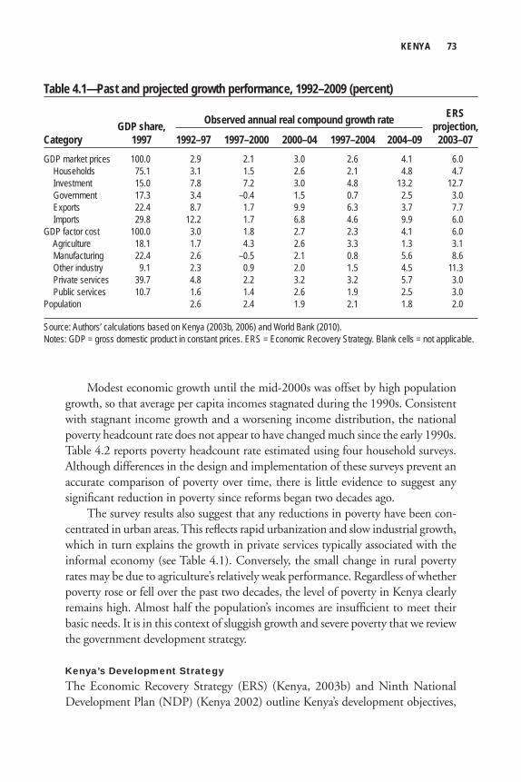
KENYA 73
Modest economic growth until the mid-2000s was offset by high population growth, so that average per capita incomes stagnated during the 1990s. Consistent with stagnant income growth and a worsening income distribution, the national poverty headcount rate does not appear to have changed much since the early 1990s. Table 4.2 reports poverty headcount rate estimated using four household surveys. Although differences in the design and implementation of these surveys prevent an accurate comparison of poverty over time, there is little evidence to suggest any signifi cant reduction in poverty since reforms began two decades ago.
The survey results also suggest that any reductions in poverty have been con-centrated in urban areas. This refl ects rapid urbanization and slow industrial growth, which in turn explains the growth in private services typically associated with the informal economy (see Table 4.1). Conversely, the small change in rural poverty rates may be due to agriculture’s relatively weak performance. Regardless of whether poverty rose or fell over the past two decades, the level of poverty in Kenya clearly remains high. Almost half the population’s incomes are insuffi cient to meet their basic needs. It is in this context of sluggish growth and severe poverty that we review the government development strategy.
Kenya’s Development StrategyThe Economic Recovery Strategy (ERS) (Kenya, 2003b) and Ninth National Development Plan (NDP) (Kenya 2002) outline Kenya’s development objectives,
Table 4.1—Past and projected growth performance, 1992–2009 (percent)
ERS GDP share, projection,Category 1997 1992–97 1997–2000 2000–04 1997–2004 2004–09 2003–07GDP market prices 100.0 2.9 2.1 3.0 2.6 4.1 6.0 Households 75.1 3.1 1.5 2.6 2.1 4.8 4.7 Investment 15.0 7.8 7.2 3.0 4.8 13.2 12.7 Government 17.3 3.4 –0.4 1.5 0.7 2.5 3.0 Exports 22.4 8.7 1.7 9.9 6.3 3.7 7.7 Imports 29.8 12.2 1.7 6.8 4.6 9.9 6.0GDP factor cost 100.0 3.0 1.8 2.7 2.3 4.1 6.0 Agriculture 18.1 1.7 4.3 2.6 3.3 1.3 3.1 Manufacturing 22.4 2.6 –0.5 2.1 0.8 5.6 8.6 Other industry 9.1 2.3 0.9 2.0 1.5 4.5 11.3 Private services 39.7 4.8 2.2 3.2 3.2 5.7 3.0 Public services 10.7 1.6 1.4 2.6 1.9 2.5 3.0Population 2.6 2.4 1.9 2.1 1.8 2.0
Source: Authors’ calculations based on Kenya (2003b, 2006) and World Bank (2010).Notes: GDP = gross domestic product in constant prices. ERS = Economic Recovery Strategy. Blank cells = not applicable.
Observed annual real compound growth rate
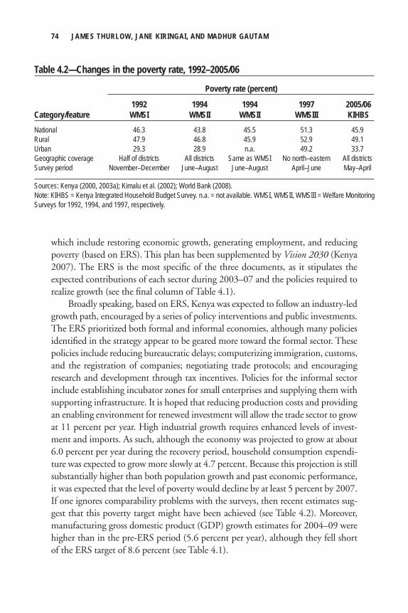
74 JAMES THURLOW, JANE KIRINGAI, AND MADHUR GAUTAM
which include restoring economic growth, generating employment, and reducing poverty (based on ERS). This plan has been supplemented by Vision 2030 (Kenya 2007). The ERS is the most specifi c of the three documents, as it stipulates the expected contributions of each sector during 2003–07 and the policies required to realize growth (see the fi nal column of Table 4.1).
Broadly speaking, based on ERS, Kenya was expected to follow an industry-led growth path, encouraged by a series of policy interventions and public investments. The ERS prioritized both formal and informal economies, although many policies identifi ed in the strategy appear to be geared more toward the formal sector. These policies include reducing bureaucratic delays; computerizing immigration, customs, and the registration of companies; negotiating trade protocols; and encouraging research and development through tax incentives. Policies for the informal sector include establishing incubator zones for small enterprises and supplying them with supporting infrastructure. It is hoped that reducing production costs and providing an enabling environment for renewed investment will allow the trade sector to grow at 11 percent per year. High industrial growth requires enhanced levels of invest-ment and imports. As such, although the economy was projected to grow at about 6.0 percent per year during the recovery period, household consumption expendi-ture was expected to grow more slowly at 4.7 percent. Because this projection is still substantially higher than both population growth and past economic performance, it was expected that the level of poverty would decline by at least 5 percent by 2007. If one ignores comparability problems with the surveys, then recent estimates sug-gest that this poverty target might have been achieved (see Table 4.2). Moreover, manufacturing gross domestic product (GDP) growth estimates for 2004–09 were higher than in the pre-ERS period (5.6 percent per year), although they fell short of the ERS target of 8.6 percent (see Table 4.1).
Table 4.2—Changes in the poverty rate, 1992–2005/06
Poverty rate (percent)
1992 1994 1994 1997 2005/06Category/feature WMSI WMSII WMSII WMSIII KIHBSNational 46.3 43.8 45.5 51.3 45.9Rural 47.9 46.8 45.9 52.9 49.1Urban 29.3 28.9 n.a. 49.2 33.7Geographic coverage Half of districts All districts Same as WMSI No north–eastern All districtsSurvey period November–December June–August June–August April–June May–April
Sources: Kenya (2000, 2003a); Kimalu et al. (2002); World Bank (2008).Note: KIHBS = Kenya Integrated Household Budget Survey. n.a. = not available. WMSI, WMSII, WMSIII = Welfare Monitoring Surveys for 1992, 1994, and 1997, respectively.
KENYA 75
According to both the ERS and NDP, agriculture has been expected to grow at about 3 percent per year under a series of proposed policies and investments. For crop agriculture, these include expanding extension services, improving rural roads and irrigation, and strengthening farmer organizations. The livestock sector is also targeted through increased support for the dairy sector and improved animal health services. Emphasis is placed on diversifying into new crops, such as cashew nuts, oilseeds, sorghum, and cassava. Agricultural research is directed toward ensuring the potential of these new crops, while extension services facilitate the dissemination of new technologies to farmers. Although it was hoped that these investments and policies could reverse the long-term decline in agricultural productivity, the two strategies were not particularly optimistic, as evidenced by the modest growth pro-jection of 3 percent. This projection represents a continuation of the agriculture’s poor longer-term growth performance. Moreover, even though the targeted growth rate was modest, the actual agricultural growth rate during 2004–09 was even lower, at only 1.3 percent per year. Later in this chapter we quantitatively evaluate the relationship between agricultural growth and poverty reduction.
The Role of AgricultureAgriculture is the largest sector in the Kenyan economy, generating a quarter of GDP and two-fi fths of export earnings (Kiringai, Thurlow, and Wanjala 2006). Moreover, agricultural production in Kenya is relatively diverse, particularly in export crop production. Although Kenya is well known for its rapid development of nontraditional crops, such as cut fl owers, it has continued to produce many important traditional export commodities, such as tea and coffee. In contrast, food-crop production is dominated by maize, whereas rice and wheat are heavily import dependent. Nonfarm activities, such as food processing, are as important as primary agriculture for the rural economy, generating two-thirds of rural GDP. Moreover, 85 percent of the population lives in rural areas, where agriculture and agriculture-related nonfarm activities are the primary sources of income for a majority of households.
Despite Kenya’s diversity, the agricultural sector has experienced mediocre growth over the past two decades, thus mirroring the weak overall performance of the economy. Agricultural production grew at 1 percent annually during the 1990s, driven by marginal improvements in crop yields or productivity (FAO 2010). However, this growth was well below the population growth rate of more than 2 percent. Although agricultural growth has doubled since 2000, this more recent period has been characterized by rapid cropland expansion and stagnant yields (FAO 2010). There is also variation in the performance of individual sectors. On the one hand, horticulture and export crops have grown rapidly over the past decade, with the exception of coffee (caused by a collapse in international prices).
76 JAMES THURLOW, JANE KIRINGAI, AND MADHUR GAUTAM
On the other hand, cereals and root crops performed poorly during the 1990s, and although these sectors have subsequently expanded production, they have continued to experience pronounced declines in yields. Given Kenya’s growing population and land constraints, the key challenge for accelerating agricultural growth is over-coming the long-standing and widespread deterioration of farm productivity.
Several studies have examined the determinants of agricultural productivity in Kenya. Falling yields during the early 1990s are attributed to the poor sequencing of market reforms and subsequent declines in the use of fertilizer and hybrid seeds (Karanja, Jayne, and Strasberg 1999; Odhiambo, Nyangito, and Nzuma 2004). Recent evidence suggests that fertilizer use is rising rapidly, although this trend is concentrated in favored agroecological regions (Ariga, Jayne, and Nyoro 2006). Furthermore, increased population pressure in these favorable regions has caused migration to less-favored lands, where existing technologies are often inappropriate (Nyoro and Jayne 1999). Funding for agricultural research is insuffi cient for the development of more appropriate seed varieties (Odhiambo, Nyangito, and Nzuma 2004). Accordingly, increased spending on research and the provision of extension services is identifi ed as a binding constraint to agricultural growth (Nyangito 1999). However, farmers’ knowledge of improved inputs is already widespread, suggesting that market development may be as important as extension (Nyoro, Wanzala, and Awour 2001). This is because higher input prices and lower output prices reduce the incentive for small-scale farmers to purchase fertilizer and hybrid seeds (Owuor 1999).
Increasing market access by investing in roads is considered complementary to enhancing on-farm technology. Furthermore, improved market access and com-mercialization are found to increase input use and yields for both food and cash crops (Strasberg et al. 1999). Productivity growth also depends on other forms of rural infrastructure, such as irrigation. Investments to improve water management have slowed dramatically over the past two decades, yet they remain fundamental for growth in some areas of the country (Odhiambo, Nyangito, and Nzuma 2004). Similarly, agricultural services that improve livestock management and disease con-trol are found to have a positive impact on growth (Kabubo-Mariara 2001; Karanja 2003). Finally, the literature identifi es access to credit and working capital as a constraint for rural households (Nyoro, Wanzala, and Awour 2001; Kibaara 2006). Therefore, extensive empirical evidence exists to identify the types of investments needed to enhance agricultural productivity and accelerate rural growth in Kenya.
Regional Differences in the Agricultural SystemA key fi nding in the literature on rural investment is that returns tend to vary across regions (see, for example, Fan and Rao 2003; Fan and Zhang 2008). To capture how initial economic and environmental conditions infl uence the impact of rural invest-
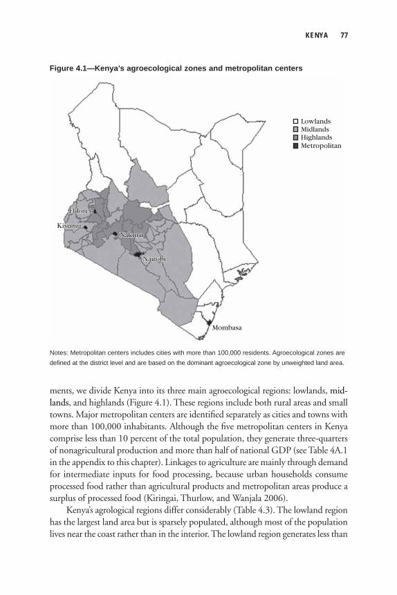
KENYA 77
ments, we divide Kenya into its three main agroecological regions: lowlands, mid-lands, and highlands (Figure 4.1). These regions include both rural areas and small towns. Major metropolitan centers are identifi ed separately as cities and towns with more than 100,000 inhabitants. Although the fi ve metropolitan centers in Kenya comprise less than 10 percent of the total population, they generate three-quarters of nonagricultural production and more than half of national GDP (see Table 4A.1 in the appendix to this chapter). Linkages to agriculture are mainly through demand for intermediate inputs for food processing, because urban households consume processed food rather than agricultural products and metropolitan areas produce a surplus of processed food (Kiringai, Thurlow, and Wanjala 2006).
Kenya’s agrological regions differ considerably (Table 4.3). The lowland region has the largest land area but is sparsely populated, although most of the population lives near the coast rather than in the interior. The lowland region generates less than
Metropolitan
Mombasa
NairobiNairobi
NakuruNakuru
EldoretEldoret
KisumuKisumu
Nairobi
Nakuru
Eldoret
Kisumu
Lowlands
HighlandsMidlands
Figure 4.1—Kenya’s agroecological zones and metropolitan centers
Notes: Metropolitan centers includes cities with more than 100,000 residents. Agroecological zones are defined at the district level and are based on the dominant agroecological zone by unweighted land area.
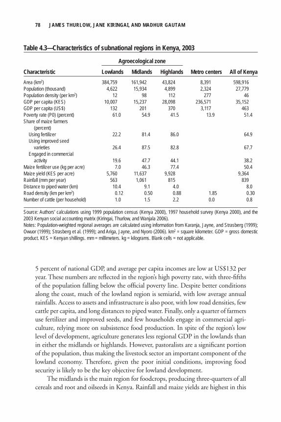
78 JAMES THURLOW, JANE KIRINGAI, AND MADHUR GAUTAM
5 percent of national GDP, and average per capita incomes are low at US$132 per year. These numbers are refl ected in the region’s high poverty rate, with three-fi fths of the population falling below the offi cial poverty line. Despite better conditions along the coast, much of the lowland region is semiarid, with low average annual rainfalls. Access to assets and infrastructure is also poor, with low road densities, few cattle per capita, and long distances to piped water. Finally, only a quarter of farmers use fertilizer and improved seeds, and few households engage in commercial agri-culture, relying more on subsistence food production. In spite of the region’s low level of development, agriculture generates less regional GDP in the lowlands than in either the midlands or highlands. However, pastoralists are a signifi cant portion of the population, thus making the livestock sector an important component of the lowland economy. Therefore, given the poor initial conditions, improving food security is likely to be the key objective for lowland development.
The midlands is the main region for foodcrops, producing three-quarters of all cereals and root and oilseeds in Kenya. Rainfall and maize yields are highest in this
Table 4.3—Characteristics of subnational regions in Kenya, 2003
Agroecological zone
Characteristic Lowlands Midlands Highlands Metro centers All of KenyaArea (km2) 384,759 161,942 43,824 8,391 598,916Population (thousand) 4,622 15,934 4,899 2,324 27,779Population density (per km2) 12 98 112 277 46GDP per capita (KES) 10,007 15,237 28,098 236,571 35,152GDP per capita (US$) 132 201 370 3,117 463Poverty rate (P0) (percent) 61.0 54.9 41.5 13.9 51.4Share of maize farmers (percent) Using fertilizer 22.2 81.4 86.0 64.9 Using improved seed varieties 26.4 87.5 82.8 67.7 Engaged in commercial activity 19.6 47.7 44.1 38.2Maize fertilizer use (kg per acre) 7.0 46.3 77.4 50.4Maize yield (KES per acre) 5,760 11,637 9,928 9,364Rainfall (mm per year) 563 1,061 815 839Distance to piped water (km) 10.4 9.1 4.0 8.0Road density (km per km2) 0.12 0.50 0.88 1.85 0.30Number of cattle (per household) 1.0 1.5 2.2 0.0 0.8
Source: Authors’ calculations using 1999 population census (Kenya 2000), 1997 household survey (Kenya 2000), and the 2003 Kenyan social accounting matrix (Kiringai, Thurlow, and Wanjala 2006). Notes: Population-weighted regional averages are calculated using information from Karanja, Jayne, and Strasberg (1999); Owuor (1999); Strasberg et al. (1999); and Ariga, Jayne, and Nyoro (2006). km2 = square kilometer. GDP = gross domestic product. KES = Kenyan shillings. mm = millimeters. kg = kilograms. Blank cells = not applicable.
KENYA 79
region, and a large share of farmers uses fertilizers and hybrid seeds. However, popu-lation density is eight times higher than in the lowlands, and land scarcity is increas-ingly a constraint to growth (Nyoro and Jayne 1999). Livestock also forms an important part of the midlands economy, although, unlike the lowlands, dairy rather than cattle farming dominates, because the midlands has better access to urban markets (Karanja 2003). Average incomes are higher and poverty is lower in the midlands than in the lowlands. However, the midlands’ large share of the popu-lation implies that almost two-thirds of the poor live in this region. The region’s dependence on agricultural incomes and its favorable initial conditions suggest that reversing falling maize yields and encouraging cash crop production are key develop-ment objectives (Mose 1999).
Finally, agrological conditions are also favorable in the highlands region, where maize yields and annual rainfall are relatively high. As in the midlands, there is widespread use of improved inputs, although only half of farmers engage in com-mercial agriculture. Unlike other regions, the highlands is heavily involved in higher value horticulture and export crops, and, despite its relatively small land area, is responsible for half of all production in these sectors. Accordingly, average incomes are higher, and poverty is substantially lower in the highlands than in the other regions. Infrastructure is also more developed, with higher road densities and better access to water. Therefore, although the nature of investments may differ, the objec-tives for the highlands are similar to those of the midlands: encourage commercial-ization and increase cash crop production.
In summary, although recent growth has been more promising, the perfor-mance of the Kenyan economy over the past decade has not been strong enough to generate signifi cant reductions in poverty. Both agricultural and industrial growth has been erratic, with periods of expansion followed by slowing growth and even stagnation. In this context, the government devised a joint strategy for economic recovery and national development, focusing primarily on industry-led growth. The strategy is less optimistic for agriculture, which is projected to continue growing at its long-term growth rate of about 3 percent per year. However, despite regional differences, the agricultural sector plays an important role throughout the Kenyan economy, both as a source of growth and as a provider of employment and incomes for a majority of the population. In light of the diverging expectations placed on agriculture and industry in the country’s development strategy, we now examine and contrast these alternative sources of growth and estimate their impacts on poverty.
The Kenyan DCGE Model A DCGE model like the one described in Chapter 2 of this volume was developed for Kenya. The model was calibrated on a detailed 2003 social accounting matrix (SAM) developed by IFPRI and the Kenya Institute for Public Policy Research and
80 JAMES THURLOW, JANE KIRINGAI, AND MADHUR GAUTAM
Analysis (KIPPRA). The SAM drew together information from a wide range of data sources, including national accounts, trade data, government budgets, indirect tax schedules, and household and labor-force surveys. Once compiled into a consistent economywide database, the SAM was balanced using cross-entropy estimation techniques. For detailed documentation of the data sources and balancing proce-dure, see Kiringai, Thurlow, and Wanjala (2006).
The SAM distinguishes between 53 agricultural and nonagricultural sectors (see Table 4A.2 in the appendix to this chapter). All sectors are further disaggregated across four subnational regions, including the three main agroecological zones (lowlands, midlands, and highlands) and the major metropolitan areas. Regional labor markets are segmented according to occupations, including skilled labor (professional workers), semiskilled (technicians, clerks, and sales workers), and unskilled workers (all other occupations and subsistence farmers). Workers are able to migrate between activities within but not between regions. Agricultural land and capital are also separated by region. Whereas agricultural land can be reallocated across crops depending on factor demands and relative factor prices, capital is fi xed by sector and, after depreciation, is supplemented by new capital from investment depending on relative sectoral profi t rates.
To capture the income and distributional impacts of alternative growth strate-gies, the DCGE model identifi es 70 representative household groups based on individual households surveyed in the 1997 Welfare Monitoring Survey (WMSIII). Households were separated by rural and urban areas, four subnational regions, and by nationally defi ned per capita expenditure deciles. Each aggregate household in the model is linked top down to their corresponding households in the survey, so that changes in per capita consumption of specifi c commodities from the DCGE model can be translated into changes in Kenya’s poverty headcount rate. The model is thus a spatially explicit representation of the Kenyan economy in 2003, and its detail allows us to conduct detailed sectoral growth simulations.
Baseline Growth ScenarioWe use the DCGE model introduced in Chapter 2 to examine the impact of alter-native sources of growth on poverty and inequality. We fi rst calibrate the model to replicate the level and structure of growth that Kenya experienced over the past fi ve years and assume such growth trends continue until 2015 (the baseline sce-nario) (see Table 4A.3 in the appendix to this chapter). We then design a set of scenarios to compare the poverty outcomes resulting from accelerating agricul-tural and industrial growth. In the second set of scenarios we assess the poverty impact of accelerating growth in different agricultural subsectors (foodcrops, livestock, and export crops).
KENYA 81
In the baseline or business-as-usual scenario, Kenya is assumed to grow at an annual rate of 3 percent between 2006 and 2015 (Table 4.4). This rate is slightly higher than what was actually experienced during the seven years (1997–2004) leading up to the base year of the model, but it is consistent with the subsequent acceleration of growth after 2000. The agricultural sector grows more rapidly than overall GDP growth at 3.3 percent, driven by the strong performance of cash crops and livestock. In contrast, foodcrops grow slowly, and food processing in the manu-facturing sector stagnates. The baseline scenario assumes a more balanced structure of growth. Manufacturing grows at 2.2 percent per year during 2006–25, which is in line with more recent trends and the observed investment growth. Services also follow past trends, with private and public services growing at 3.3 and 2.0 percent per year, respectively.
Although the economy grows at 3 percent per year, household consumption expenditure rises by only 0.9 percent in per capita terms. This rate is higher than the per capita consumption growth experienced during the 1990s. Given rising per capita consumption, income-based poverty declines slightly in the baseline. The national incidence of poverty falls from 51.3 percent in 2003 to 48.1 percent in 2015 (Table 4.5). However, this aggregate decline hides the continued rise in urban poverty, from 47.6 percent in 2003 to 49.5 percent by 2015. With declining rural poverty during the same period, the baseline scenario suggests that, if the 1997–2004 growth rates had been maintained, then urban poverty would be higher than rural poverty by 2015.
We also measure the effectiveness of baseline growth to reduce poverty using the poverty–growth elasticity (Ravallion and Chen 2003). The value of this elasticity is low at –0.38 (see Table 4.5). Thus, 1 percent growth in per capita GDP leads to a 0.38 percent decline in the poverty rate. With this elasticity it would require an annual GDP growth of 10.3 percent in 2006–15 to achieve the fi rst Millennium Development Goal (MDG1) of halving 1992 poverty by 2015 (that is, to reach a poverty rate of 22.2 percent). Required growth for MDG1 is based on a balanced growth assumption, and poverty–growth elasticity is assumed to remain constant at –0.38. In the next section we assess whether there are alternative sources of growth that would be more pro-poor than the current baseline.
Accelerated Growth Scenarios
Comparing Agriculture and Industry-Led GrowthThe impact of agricultural and industrial growth on poverty is examined by accel-erating the overall GDP growth rate from its current 3 percent to 4 percent per year. Two scenarios are presented, in which the source of this additional growth differs.
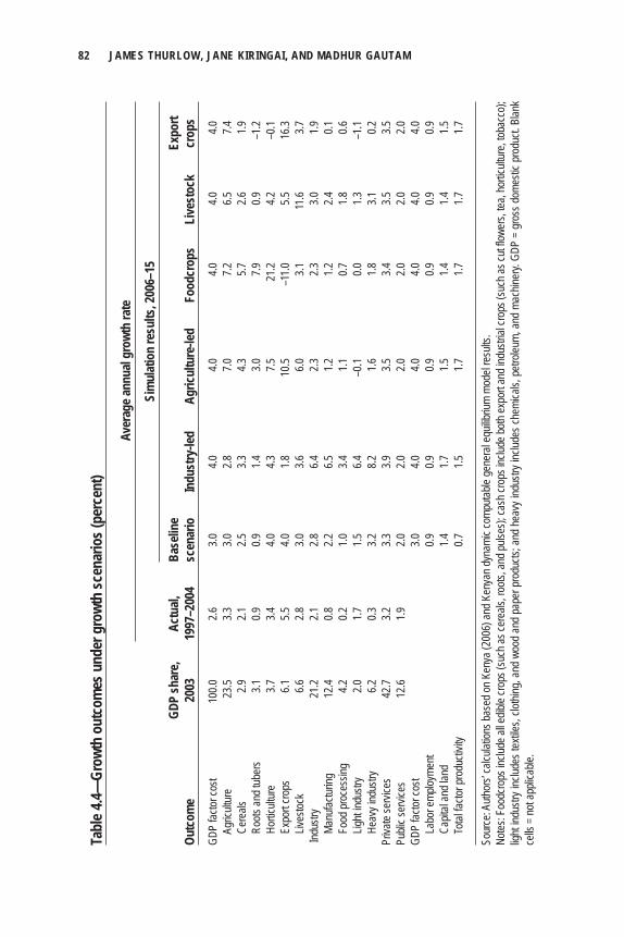
82 JAMES THURLOW, JANE KIRINGAI, AND MADHUR GAUTAM
Tabl
e 4.4—
Grow
th o
utco
mes
und
er g
rowt
h sc
enar
ios (
perc
ent)
Av
erag
e ann
ual g
rowt
h ra
te
Si
mul
atio
n re
sults
, 200
6–15
GD
P sh
are,
Actu
al,
Base
line
Expo
rtOu
tcom
e 20
03
1997
–200
4 sc
enar
io
Indu
stry
-led
Agric
ultu
re-le
d Fo
odcr
ops
Live
stoc
k cr
ops
GDP
factor
cost
100.0
2.6
3.0
4.0
4.0
4.0
4.0
4.0
Ag
ricult
ure
23.5
3.3
3.0
2.8
7.0
7.2
6.5
7.4
Cere
als
2.9
2.1
2.5
3.3
4.3
5.7
2.6
1.9
Roots
and t
uber
s 3.1
0.9
0.9
1.4
3.0
7.9
0.9
–1
.2
Hortic
ultur
e 3.7
3.4
4.0
4.3
7.5
21
.2 4.2
–0
.1
Expo
rt cro
ps
6.1
5.5
4.0
1.8
10.5
–11.0
5.5
16
.3
Lives
tock
6.6
2.8
3.0
3.6
6.0
3.1
11.6
3.7 In
dustr
y 21
.2 2.1
2.8
6.4
2.3
2.3
3.0
1.9
Ma
nufac
turing
12
.4 0.8
2.2
6.5
1.2
1.2
2.4
0.1
Fo
od pr
oces
sing
4.2
0.2
1.0
3.4
1.1
0.7
1.8
0.6
Light
indus
try
2.0
1.7
1.5
6.4
–0.1
0.0
1.3
–1.1
He
avy i
ndus
try
6.2
0.3
3.2
8.2
1.6
1.8
3.1
0.2Pr
ivate
servi
ces
42.7
3.2
3.3
3.9
3.5
3.4
3.5
3.5Pu
blic s
ervic
es
12.6
1.9
2.0
2.0
2.0
2.0
2.0
2.0GD
P fac
tor co
st
3.0
4.0
4.0
4.0
4.0
4.0
La
bor e
mploy
ment
0.9
0.9
0.9
0.9
0.9
0.9
Capit
al an
d lan
d
1.4
1.7
1.5
1.4
1.4
1.5
To
tal fa
ctor p
rodu
ctivit
y
0.7
1.5
1.7
1.7
1.7
1.7
Sour
ce: A
uthor
s’ ca
lculat
ions b
ased
on K
enya
(200
6) an
d Ken
yan d
ynam
ic co
mputa
ble ge
nera
l equ
ilibriu
m mo
del re
sults
.No
tes: F
oodc
rops
inclu
de al
l edib
le cro
ps (s
uch a
s cer
eals,
roots
, and
pulse
s); ca
sh cr
ops i
nclud
e both
expo
rt an
d ind
ustria
l cro
ps (s
uch a
s cut
flowe
rs, te
a, ho
rticult
ure,
tobac
co);
light
indus
try in
clude
s tex
tiles,
clothi
ng, a
nd w
ood
and
pape
r pro
ducts
; and
hea
vy in
dustr
y inc
ludes
chem
icals,
petr
oleum
, and
mac
hiner
y. GD
P =
gros
s dom
estic
pro
duct.
Blan
k ce
lls =
not a
pplic
able.
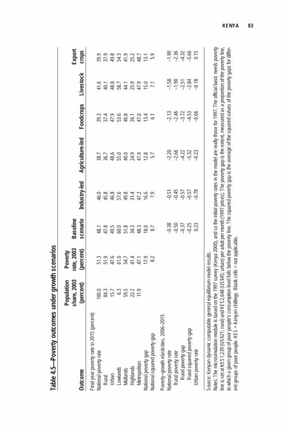
KENYA 83
Tabl
e 4.5—
Pove
rty o
utco
mes
und
er g
rowt
h sc
enar
ios
Po
pulat
ion
Pove
rty
shar
e, 20
03
rate
, 200
3 Ba
selin
e
Ex
port
Outc
ome
(per
cent
) (p
erce
nt)
scen
ario
In
dust
ry-le
d Ag
ricul
ture
-led
Food
crop
s Li
vest
ock
crop
sFin
al ye
ar po
verty
rate
in 20
15 (p
erce
nt)Na
tiona
l pov
erty
rate
100.0
51
.3 48
.1 46
.0 38
.7 39
.3 41
.6 39
.9
Rura
l 84
.3 51
.9 47
.8 45
.8 36
.7 37
.4 40
.1 37
.9
Urba
n 15
.7 47
.6 49
.5 46
.8 48
.6 47
.9 48
.8 49
.8
Lowl
ands
6.3
61
.0 60
.0 57
.6 55
.0 53
.6 58
.7 54
.3
Midla
nds
59.5
54.7
51.8
49.8
40.0
40.8
44.1
41.9
Hi
ghlan
ds
22.2
41.4
34.3
31.4
24.9
26.1
25.9
25.2
Me
tropo
litan
11.9
47.1
48.3
47.2
47.9
47.0
47.9
48.7
Natio
nal p
over
ty ga
p
17.9
18.0
16.6
12.8
13.4
15.0
13.1
Natio
nal s
quar
ed po
verty
gap
8.2
8.7
7.9
5.7
6.1
7.1
5.9
Pove
rty–g
rowt
h elas
ticitie
s, 20
06–2
015
Natio
nal p
over
ty ra
te
–0.38
–0
.51
–2.20
–2
.13
–1.58
–1
.90
Rura
l pov
erty
rate
–0.50
–0
.45
–2.66
–2
.46
–1.90
–2
.36
Ru
ral p
over
ty ga
p
–0
.37
–0.57
–4
.22
–3.72
–2
.51
–4.32
Rura
l squ
ared
pove
rty ga
p
–0
.25
–0.57
–5
.32
–4.53
–2
.84
–5.66
Ur
ban p
over
ty ra
te
0.2
3 –0
.78
–0.23
–0
.66
–0.18
0.1
5
Sour
ce: K
enya
n dyn
amic
comp
utable
gene
ral e
quilib
rium
mode
l resu
lts.
Notes
: The
micr
osim
ulatio
n mod
ule is
base
d on t
he 19
97 su
rvey (
Keny
a 200
0), a
nd so
the i
nitial
pove
rty ra
tes in
the m
odel
are r
eally
thos
e for
1997
. The
offic
ial ba
sic ne
eds p
over
ty lin
e is s
et at
KES1
,239 (
US$2
1; ru
ral) a
nd K
ES2,6
48 (U
S$45
; urb
an) p
er ad
ult pe
r mon
th (1
997 p
rices
). The
pove
rty ga
p is t
he ex
tent, m
easu
red a
s a pr
opor
tion o
f the p
over
ty lin
e, to
which
a giv
en gr
oup o
f poo
r peo
ple’s
cons
umpti
on le
vel fa
lls be
low th
e pov
erty
line.
The s
quar
ed po
verty
gap i
s the
aver
age o
f the s
quar
ed va
lues o
f the p
over
ty ga
ps fo
r diffe
r-en
t gro
ups o
f poo
r peo
ple. K
ES =
Ken
yan s
hillin
gs. B
lank c
ells =
not a
pplic
able.
84 JAMES THURLOW, JANE KIRINGAI, AND MADHUR GAUTAM
In the agriculture-led scenario, growth in the agricultural and food processing sec-tors is increased, while additional growth in the industry-led scenario comes from mining, nonfood manufacturing, and construction. Although the two scenarios try to target the same overall GDP growth rate, the required sectoral growth rates differ in the two scenarios because of their sizes and growth linkages in the economy. For instance, to raise GDP growth rate from 3 to 4 percent per year, the growth rate of agriculture has to increase from the baseline 3.3 percent to 7.0 percent in the agriculture-led growth scenario (see Table 4.4). Conversely, in the industry-led scenario, manufacturing growth increases from 2.2 to 6.5 percent per year to have a similar overall GDP growth outcome as the agriculture-led growth scenario.
Although we assume that accelerated agricultural growth occurs in all agricul-tural subsectors in the agriculture-led scenario, export crops are assumed to grow faster than other agricultural subsectors. This might possibly be due to better foreign market opportunities, such that production of export crops is not necessarily con-strained by domestic demand. In the agriculture-led scenario, rural households benefi t directly from increased agricultural incomes. In contrast, the benefi t for urban households is mainly through lower food prices, and hence an increase in their consumption levels at a given income (that is, real consumption). Therefore, in the agriculture-led scenario poverty in both rural and urban areas declines, although rural poverty rate falls more (see Table 4.5). Rising incomes and expendi-tures are particularly pronounced among the poorest populations, as seen by the larger decline in both the depth and severity of poverty.
In contrast, the benefi ts of faster nonfood manufacturing growth in both the formal and informal sectors in the industry-led scenario are concentrated among the less-poor households. Although faster growth in the labor-intensive light indus-try and construction sectors does benefi t poorer urban households, urban poverty in the industry-led scenario declines only slightly faster than under agriculture-led growth. This modest difference is because poor urban households are less likely to be employed in the mining and heavy manufacturing sectors and hence only benefi t indirectly through higher economywide growth in the informal service sec-tors. However, the overall effect of accelerating growth in light manufacturing and construction and the spillover into services is enough to ensure that the informal economy grows alongside the formal economy. This parallel growth drives the decline in urban poverty but limits any positive spillovers to rural households. Accordingly, if an additional 1 percent of overall GDP growth is led by faster growth in nonfood manufacturing sectors, then the national poverty rate declines by 2.1 percentage points more than that in the baseline by 2015. Conversely, national poverty declines by 9.4 percentage points if the same level of national growth is led by the agricultural sector. This difference is refl ected in the poverty–growth elastic-
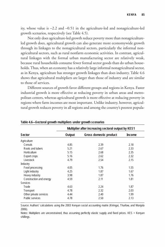
KENYA 85
ity, whose value is –2.2 and –0.51 in the agriculture-led and nonagriculture-led growth scenarios, respectively (see Table 4.5).
Not only does agriculture-led growth reduce poverty more than nonagriculture-led growth does, agricultural growth can also generate more economywide growth through its linkages to the nonagricultural sectors, particularly the informal non-agricultural sectors, such as rural nonfarm economic activities. In contrast, agricul-tural linkages with the formal urban manufacturing sector are relatively weak, because rural households consume fewer formal sector goods than do urban house-holds. Thus, when an economy has a relatively large informal nonagricultural sector, as in Kenya, agriculture has stronger growth linkages than does industry. Table 4.6 shows that agricultural multipliers are larger than those of industry and are similar to those of services.
Different sources of growth favor different groups and regions in Kenya. Faster industrial growth is more effective at reducing poverty in urban areas and metro-politan centers, whereas agricultural growth is more effective at reducing poverty in regions where farm incomes are most important. Unlike industry, however, agricul-tural growth reduces poverty in all regions and among the country’s poorest popula-
Table 4.6—Sectoral growth multipliers under growth scenarios
Multiplier after increasing sectoral output by KES1
Sector Output Gross domestic product IncomeAgriculture Cereals 4.85 2.39 2.18 Roots and tubers 5.21 2.67 2.33 Horticulture 5.15 2.68 2.35 Export crops 5.16 2.62 2.32 Livestock 4.79 2.54 2.15Industry Food processing 4.05 1.76 1.55 Light industry 4.25 1.87 1.67 Heavy industry 3.98 1.87 1.76 Construction and energy 4.59 2.11 1.81Services Trade 4.63 2.24 1.87 Transport 4.78 2.32 2.03 Other private services 4.44 2.40 1.99 Public services 4.78 2.50 2.13
Source: Authors’ calculations using the 2003 Kenyan social accounting matrix (Kiringai, Thurlow, and Wanjala 2006).Notes: Multipliers are unconstrained, thus assuming perfectly elastic supply and fixed prices. KES = Kenyan shillings.
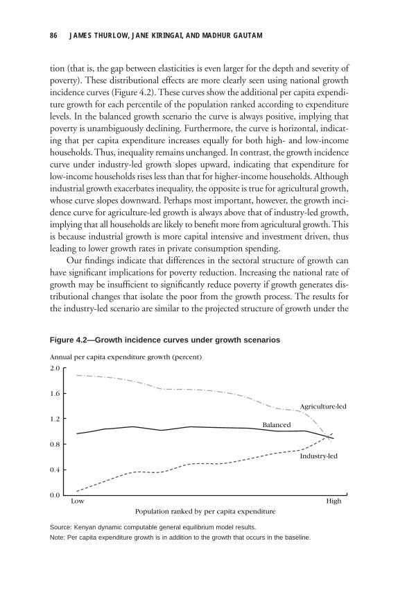
86 JAMES THURLOW, JANE KIRINGAI, AND MADHUR GAUTAM
tion (that is, the gap between elasticities is even larger for the depth and severity of poverty). These distributional effects are more clearly seen using national growth incidence curves (Figure 4.2). These curves show the additional per capita expendi-ture growth for each percentile of the population ranked according to expenditure levels. In the balanced growth scenario the curve is always positive, implying that poverty is unambiguously declining. Furthermore, the curve is horizontal, indicat-ing that per capita expenditure increases equally for both high- and low-income households. Thus, inequality remains unchanged. In contrast, the growth incidence curve under industry-led growth slopes upward, indicating that expenditure for low-income households rises less than that for higher-income households. Although industrial growth exacerbates inequality, the opposite is true for agricultural growth, whose curve slopes downward. Perhaps most important, however, the growth inci-dence curve for agriculture-led growth is always above that of industry-led growth, implying that all households are likely to benefi t more from agricultural growth. This is because industrial growth is more capital intensive and investment driven, thus leading to lower growth rates in private consumption spending.
Our fi ndings indicate that differences in the sectoral structure of growth can have signifi cant implications for poverty reduction. Increasing the national rate of growth may be insuffi cient to signifi cantly reduce poverty if growth generates dis-tributional changes that isolate the poor from the growth process. The results for the industry-led scenario are similar to the projected structure of growth under the
Annual per capita expenditure growth (percent)
2.0
0.0Low High
Industry-led
Agriculture-led
Balanced
Population ranked by per capita expenditure
0.8
1.2
1.6
0.4
Figure 4.2—Growth incidence curves under growth scenarios
Source: Kenyan dynamic computable general equilibrium model results.Note: Per capita expenditure growth is in addition to the growth that occurs in the baseline.
KENYA 87
government’s national growth strategy ERS. Therefore, given its focus on industrial growth, the ERS is likely to produce poverty outcomes similar to the industry-led scenario presented here. Our results also indicate that industry-led growth could worsen income inequality, which is already high in Kenya. This increase in inequality was indeed observed in the few years after the ERS was implemented, with poverty falling only slightly in rural areas but more substantially in urban ones (see Table 4.2). However, caution should be exercised, because the 2005/06 survey may not have allowed suffi cient time for ERS to be properly implemented, and so it may refl ect the effects of policies and events prior to ERS.
Although agricultural growth may be more pro-poor than industrial growth, no single source of growth is equally effective at reducing poverty in all areas and regions of the country. Nor should the benefi ts of agricultural or industrial growth be seen to affect only rural and urban households, respectively. In the case of Kenya, industrial growth linkages generate positive spillovers to the rural nonfarm economy, and agriculture’s growth linkages raise real urban incomes, especially in the informal economy. Agricultural and industrial growth are therefore not mutually exclusive. However, our results suggest that agricultural growth should receive greater empha-sis in Kenya’s future growth strategy if the country is to achieve more equitable outcomes. Accordingly, the rest of this chapter focuses on accelerating growth in the agricultural sector.
Decomposing the Contribution of AgricultureNow we look within Kenya’s agricultural development and decompose the potential contribution of different agricultural subsectors to growth and poverty reduction. The effectiveness of the foodcrop, livestock, and export crop subsectors in reducing poverty is again examined by raising the overall GDP growth rate from 3 to 4 percent per year. This is done by increasing their sectoral growth rates via higher productivity. Three simulations are considered: (1) accelerated growth in foodcrops, (2) accelerated growth in the livestock and dairy sectors, and (3) accelerated growth in export crops. In these simulations, foodcrops include maize, sorghum, and millet; export crops include traditional and nontraditional crops, such as tea, cotton, coffee, and horticulture; and livestock includes beef, poultry, dairy, and other livestock-related activities. Understanding the relationship of these subsectors to pro-poor growth is especially important for Kenya, whose agricultural growth in recent years has been characterized by a relatively rapid expansion in export crops and livestock but modest growth in foodcrops and downstream processing.
Agriculture’s overall growth rate in the foodcrop scenario increases from 3.0 to 7.2 percent to generate the additional 1 percent in overall GDP growth (see Table 4.4). The additional agricultural growth is higher in the export crop scenario, and the effect of rapidly rising agricultural exports is an appreciation of the real exchange
88 JAMES THURLOW, JANE KIRINGAI, AND MADHUR GAUTAM
rate, which undermines the competitiveness of other agricultural and manufactur-ing exports. Manufacturing growth therefore declines signifi cantly in the export crop scenario. However, despite improved agricultural productivity, rapid growth in foodcrops creates greater competition for agricultural resources, especially land and rural labor, and this reduces the availability of these resources for other agricultural sectors. Accordingly, export crop growth reverses from 4 percent in the baseline scenario to –11 percent in the foodcrop scenario. Therefore, there is defi nite com-petition over resources between foodcrops and export crops. Shifts in the composi-tion of agricultural growth also infl uence how households benefi t from growth. These differences remain small at the national level, with foodcrop growth generat-ing slightly better poverty outcomes than does growth in export crops (Figure 4.3). However, at the subnational level there are more signifi cant differences, with the lowlands and midlands benefi ting more from foodcrop expansion than the high-lands do, which in turn benefi t more from export crops.
Accelerating livestock production in the livestock scenario does not lead to pronounced resource competition with other agricultural sectors. Growth in the dairy sector favors the highland region. However, the impact on poverty resulting from accelerated livestock growth is smaller than under either foodcrop or export crop growth, especially for the depth and severity of poverty. This relationship is evident in the relative sizes of the poverty–growth elasticities (see Table 4.6). Although all three scenarios have large elasticities, it is foodcrop production that strengthens the growth–poverty relationship the most. However, even though this is true for the lowlands and midlands, it is not true for the highlands, where the growth–poverty relationship is weakened by an expansion of foodcrops (at the expense of cash crops). In contrast, households in the highlands benefi t more in the cash crop and livestock scenarios, albeit at the expense of lowland growth and poverty. Therefore, although the previous section found that agricultural growth is more pro-poor than is industrial growth, there are still trade-offs in agriculture that can result in signifi cant distributional changes.
In summary, a growth strategy that seeks to share the benefi ts of growth among households throughout the country cannot focus agricultural growth only in certain sectors. Such a narrow approach may successfully reduce poverty in the short term as incomes rise for households in those regions with appropriate conditions. However, national poverty reduction would taper off, because households in the less-favored regions are effectively isolated from the growth process. This differential effect is especially true in the lagging lowlands. Promoting only certain sectors with-out considering distributional change and regional differences can effectively exclude sections of the population from the benefi ts of growth. It should also be noted that the growth rates that would be required from export crops and horticulture if they were solely responsible for generating additional GDP growth are unrealistically
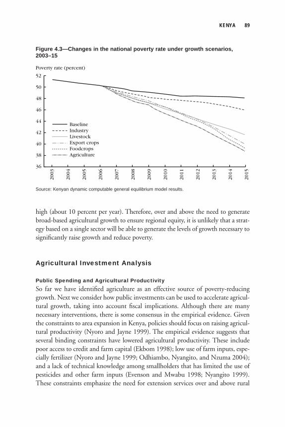
KENYA 89
high (about 10 percent per year). Therefore, over and above the need to generate broad-based agricultural growth to ensure regional equity, it is unlikely that a strat-egy based on a single sector will be able to generate the levels of growth necessary to signifi cantly raise growth and reduce poverty.
Agricultural Investment Analysis
Public Spending and Agricultural ProductivitySo far we have identifi ed agriculture as an effective source of poverty-reducing growth. Next we consider how public investments can be used to accelerate agricul-tural growth, taking into account fi scal implications. Although there are many necessary interventions, there is some consensus in the empirical evidence. Given the constraints to area expansion in Kenya, policies should focus on raising agricul-tural productivity (Nyoro and Jayne 1999). The empirical evidence suggests that several binding constraints have lowered agricultural productivity. These include poor access to credit and farm capital (Ekbom 1998); low use of farm inputs, espe-cially fertilizer (Nyoro and Jayne 1999; Odhiambo, Nyangito, and Nzuma 2004); and a lack of technical knowledge among smallholders that has limited the use of pesticides and other farm inputs (Evenson and Mwabu 1998; Nyangito 1999). These constraints emphasize the need for extension services over and above rural
Poverty rate (percent)
52
36
2015
2014
Export cropsFoodcropsAgriculture
LivestockIndustryBaseline
40
42
44
46
48
50
38
2013
2012
2011
2010
2009
2008
2007
2006
2005
2004
2003
Figure 4.3—Changes in the national poverty rate under growth scenarios, 2003–15
Source: Kenyan dynamic computable general equilibrium model results.
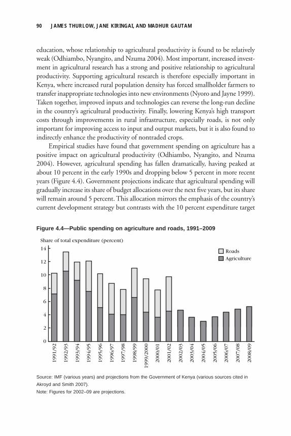
90 JAMES THURLOW, JANE KIRINGAI, AND MADHUR GAUTAM
education, whose relationship to agricultural productivity is found to be relatively weak (Odhiambo, Nyangito, and Nzuma 2004). Most important, increased invest-ment in agricultural research has a strong and positive relationship to agricultural productivity. Supporting agricultural research is therefore especially important in Kenya, where increased rural population density has forced smallholder farmers to transfer inappropriate technologies into new environments (Nyoro and Jayne 1999). Taken together, improved inputs and technologies can reverse the long-run decline in the country’s agricultural productivity. Finally, lowering Kenya’s high transport costs through improvements in rural infrastructure, especially roads, is not only important for improving access to input and output markets, but it is also found to indirectly enhance the productivity of nontraded crops.
Empirical studies have found that government spending on agriculture has a positive impact on agricultural productivity (Odhiambo, Nyangito, and Nzuma 2004). However, agricultural spending has fallen dramatically, having peaked at about 10 percent in the early 1990s and dropping below 5 percent in more recent years (Figure 4.4). Government projections indicate that agricultural spending will gradually increase its share of budget allocations over the next fi ve years, but its share will remain around 5 percent. This allocation mirrors the emphasis of the country’s current development strategy but contrasts with the 10 percent expenditure target
Share of total expenditure (percent)
14
0
6
1991
/92
8
10
12
4
2
RoadsAgriculture
1994
/95
1997
/98
2000
/01
2003
/04
2006
/07
1992
/93
1995
/96
1998
/99
2001
/02
2004
/05
2007
/08
1993
/94
1996
/97
1999
/200
0
2002
/03
2005
/06
2008
/09
Figure 4.4—Public spending on agriculture and roads, 1991–2009
Source: IMF (various years) and projections from the Government of Kenya (various sources cited in Akroyd and Smith 2007).Note: Figures for 2002–09 are projections.
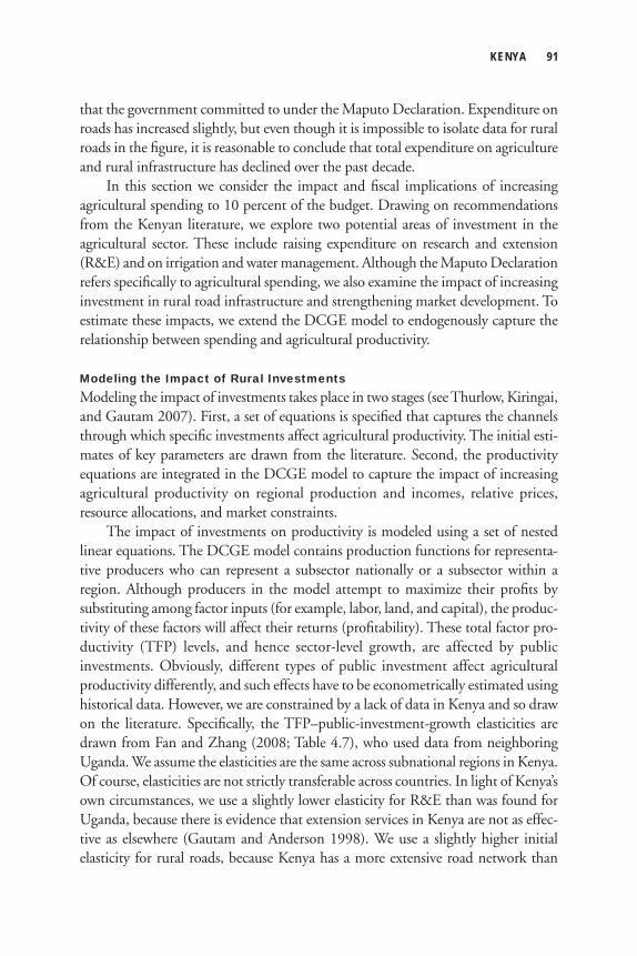
KENYA 91
that the government committed to under the Maputo Declaration. Expenditure on roads has increased slightly, but even though it is impossible to isolate data for rural roads in the fi gure, it is reasonable to conclude that total expenditure on agriculture and rural infrastructure has declined over the past decade.
In this section we consider the impact and fi scal implications of increasing agricultural spending to 10 percent of the budget. Drawing on recommendations from the Kenyan literature, we explore two potential areas of investment in the agricultural sector. These include raising expenditure on research and extension (R&E) and on irrigation and water management. Although the Maputo Declaration refers specifi cally to agricultural spending, we also examine the impact of increasing investment in rural road infrastructure and strengthening market development. To estimate these impacts, we extend the DCGE model to endogenously capture the relationship between spending and agricultural productivity.
Modeling the Impact of Rural InvestmentsModeling the impact of investments takes place in two stages (see Thurlow, Kiringai, and Gautam 2007). First, a set of equations is specifi ed that captures the channels through which specifi c investments affect agricultural productivity. The initial esti-mates of key parameters are drawn from the literature. Second, the productivity equations are integrated in the DCGE model to capture the impact of increasing agricultural productivity on regional production and incomes, relative prices, resource allocations, and market constraints.
The impact of investments on productivity is modeled using a set of nested linear equations. The DCGE model contains production functions for representa-tive producers who can represent a subsector nationally or a subsector within a region. Although producers in the model attempt to maximize their profi ts by substituting among factor inputs (for example, labor, land, and capital), the produc-tivity of these factors will affect their returns (profi tability). These total factor pro-ductivity (TFP) levels, and hence sector-level growth, are affected by public investments. Obviously, different types of public investment affect agricultural productivity differently, and such effects have to be econometrically estimated using historical data. However, we are constrained by a lack of data in Kenya and so draw on the literature. Specifi cally, the TFP–public-investment-growth elasticities are drawn from Fan and Zhang (2008; Table 4.7), who used data from neighboring Uganda. We assume the elasticities are the same across subnational regions in Kenya. Of course, elasticities are not strictly transferable across countries. In light of Kenya’s own circumstances, we use a slightly lower elasticity for R&E than was found for Uganda, because there is evidence that extension services in Kenya are not as effec-tive as elsewhere (Gautam and Anderson 1998). We use a slightly higher initial elasticity for rural roads, because Kenya has a more extensive road network than
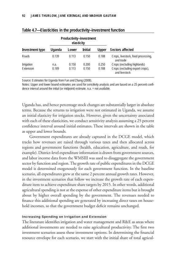
92 JAMES THURLOW, JANE KIRINGAI, AND MADHUR GAUTAM
Uganda has, and hence percentage stock changes are substantially larger in absolute terms. Because the returns to irrigation were not estimated in Uganda, we assume an initial elasticity for irrigation stocks. However, given the uncertainty associated with each of these elasticities, we conduct sensitivity analysis assuming a 25 percent confi dence interval around initial estimates. These intervals are shown in the table as upper and lower bounds.
Government expenditures are already captured in the DCGE model, which tracks how revenues are raised through various taxes and then allocated across regions and government functions (health, education, agriculture, and roads, for example). District-level expenditure information is drawn from government sources, and labor income data from the WMSIII was used to disaggregate the government sector by function and region. The growth rate of public expenditures in the DCGE model is determined exogenously for each government function. In the baseline scenario, all expenditures grew at the same 2 percent annual growth rates. However, in the investment scenarios that follow we increase the growth rate of each expen-diture item to achieve expenditure share targets by 2015. In other words, additional agricultural spending is not at the expense of other expenditure items but is brought about by higher overall spending by the government. The revenues needed to fi nance this additional spending are generated by increasing direct taxes on house-hold incomes, so that the government budget defi cit remains unchanged.
Increasing Spending on Irrigation and Extension The literature identifi es irrigation and water management and R&E as areas where additional investments are needed to raise agricultural productivity. The fi rst two investment scenarios assess these investment options. In determining the fi nancial resource envelope for each scenario, we start with the initial share of total agricul-
Table 4.7—Elasticities in the productivity–investment function
Productivity–investment elasticity
Investment type Uganda Lower Initial Upper Sectors affectedRoads 0.139 0.113 0.150 0.188 Crops, livestock, food processing, and trade Irrigation n.a. 0.150 0.200 0.250 Crops (excluding highlands) Extension 0.189 0.113 0.150 0.188 Crops (excluding export crops), and livestock
Source: Estimates for Uganda from Fan and Zhang (2008). Notes: Upper and lower bound estimates are used for sensitivity analysis and are based on a 25 percent confi-dence interval around the initial (or midpoint) estimate. n.a. = not available.
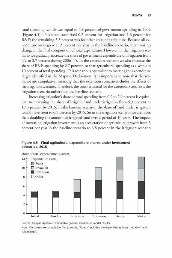
KENYA 93
tural spending, which was equal to 4.8 percent of government spending in 2002 (Figure 4.5). This share comprised 0.2 percent for irrigation and 1.3 percent for R&E; the remaining 3.3 percent was for other areas of agriculture. Because all ex-penditure areas grew at 2 percent per year in the baseline scenario, there was no change in the fi nal composition of total expenditure. However, in the irrigation sce-nario we gradually increase the share of government expenditure on irrigation from 0.2 to 2.7 percent during 2006–15. In the extension scenario we also increase the share of R&E spending by 2.7 percent, so that agricultural spending as a whole is 10 percent of total spending. This scenario is equivalent to meeting the expenditure target identifi ed in the Maputo Declaration. It is important to note that the sce-narios are cumulative, meaning that the extension scenario includes the effects of the irrigation scenario. Therefore, the counterfactual for the extension scenario is the irrigation scenario rather than the baseline scenario.
Increasing irrigation’s share of total spending from 0.2 to 2.9 percent is equiva-lent to increasing the share of irrigable land under irrigation from 5.3 percent to 19.3 percent by 2015. In the baseline scenario, the share of land under irrigation would have risen to 6.9 percent by 2015. So in the irrigation scenario we are more than doubling the amount of irrigated land over a period of 10 years. The impact of increasing irrigation investment is an acceleration of agricultural growth from 3 percent per year in the baseline scenario to 3.8 percent in the irrigation scenario
Share of total expenditure (percent)
12
0
6
Initial
8
10
4
2
Baseline Irrigation Extension Roads Market
Other
Roads
Expenditure items
Extension
Irrigation
Figure 4.5—Final agricultural expenditure shares under investment scenarios, 2015
Source: Kenyan dynamic computable general equilibrium model results.Note: Outcomes are cumulative (for example, “Roads” includes the expenditures from “Irrigation” and “Extension”).
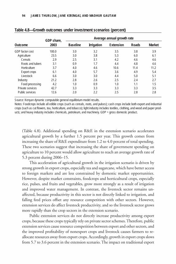
94 JAMES THURLOW, JANE KIRINGAI, AND MADHUR GAUTAM
(Table 4.8). Additional spending on R&E in the extension scenario accelerates agricultural growth by a further 1.5 percent per year. This growth comes from increasing the share of R&E expenditure from 1.2 to 4.0 percent of total spending. These two scenarios suggest that increasing the share of government spending on agriculture to 10 percent would allow agriculture to reach an average growth rate of 5.3 percent during 2006–15.
This acceleration of agricultural growth in the irrigation scenario is driven by strong growth in export crops, especially tea and sugarcane, which have better access to foreign markets and are less constrained by domestic market opportunities. However, despite market constraints, foodcrops and horticultural crops, especially rice, pulses, and fruits and vegetables, grow more strongly as a result of irrigation and improved water management. In contrast, the livestock sector remains un-affected, because productivity in this sector is not directly linked to irrigation, and falling feed prices offset any resource competition with other sectors. However, extension services do affect livestock productivity, and so the livestock sector grows more rapidly than the crop sectors in the extension scenario.
Public extension services do not directly increase productivity among export crops, because these crops typically rely on private sector schemes. Therefore, public extension services cause resource competition between export and other sectors, and the improved profi tability of nonexport crops and livestock causes farmers to re-allocate resources away from export crops. Accordingly, growth in export crops slows from 5.7 to 3.6 percent in the extension scenario. The impact on traditional export
Table 4.8—Growth outcomes under investment scenarios (percent)
GDP share,Outcome 2003 Baseline Irrigation Extension Roads MarketGDP factor cost 100.0 3.0 3.2 3.5 3.8 3.9 Agriculture 23.5 3.0 3.8 5.3 6.0 6.1 Cereals 2.9 2.5 3.1 4.2 4.6 4.6 Roots and tubers 3.1 0.9 1.7 4.4 4.8 4.6 Horticulture 3.7 4.0 4.6 10.6 11.4 11.2 Export crops 6.1 4.0 5.7 3.6 4.9 5.4 Livestock 6.6 3.0 3.0 4.4 5.0 5.1 Industry 21.2 2.8 2.6 2.5 2.4 2.7 Food processing 4.2 1.0 0.9 1.0 1.1 1.5 Private services 42.7 3.3 3.3 3.3 3.3 3.5 Public services 12.6 2.0 2.2 2.5 2.8 2.8
Source: Kenyan dynamic computable general equilibrium model results.Notes: Foodcrops include all edible crops (such as cereals, roots, and pulses); cash crops include both export and industrial crops (such as cut flowers, tea, horticulture, and tobacco); light industry includes textiles, clothing, and wood and paper prod-ucts; and heavy industry includes chemicals, petroleum, and machinery. GDP = gross domestic product.
Average annual growth rate
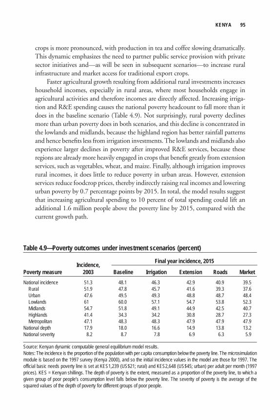
KENYA 95
crops is more pronounced, with production in tea and coffee slowing dramatically. This dynamic emphasizes the need to partner public service provision with private sector initiatives and—as will be seen in subsequent scenarios—to increase rural infrastructure and market access for traditional export crops.
Faster agricultural growth resulting from additional rural investments increases household incomes, especially in rural areas, where most households engage in agricultural activities and therefore incomes are directly affected. Increasing irriga-tion and R&E spending causes the national poverty headcount to fall more than it does in the baseline scenario (Table 4.9). Not surprisingly, rural poverty declines more than urban poverty does in both scenarios, and this decline is concentrated in the lowlands and midlands, because the highland region has better rainfall patterns and hence benefi ts less from irrigation investments. The lowlands and midlands also experience larger declines in poverty after improved R&E services, because these regions are already more heavily engaged in crops that benefi t greatly from extension services, such as vegetables, wheat, and maize. Finally, although irrigation improves rural incomes, it does little to reduce poverty in urban areas. However, extension services reduce foodcrop prices, thereby indirectly raising real incomes and lowering urban poverty by 0.7 percentage points by 2015. In total, the model results suggest that increasing agricultural spending to 10 percent of total spending could lift an additional 1.6 million people above the poverty line by 2015, compared with the current growth path.
Table 4.9—Poverty outcomes under investment scenarios (percent)
Incidence,Poverty measure 2003 Baseline Irrigation Extension Roads MarketNational incidence 51.3 48.1 46.3 42.9 40.9 39.5 Rural 51.9 47.8 45.7 41.6 39.3 37.6 Urban 47.6 49.5 49.3 48.8 48.7 48.4 Lowlands 61 60.0 57.1 54.7 53.8 52.3 Midlands 54.7 51.8 49.1 44.9 42.5 40.7 Highlands 41.4 34.3 34.2 30.8 28.7 27.3 Metropolitan 47.1 48.3 48.3 47.9 47.9 47.9National depth 17.9 18.0 16.6 14.9 13.8 13.2National severity 8.2 8.7 7.8 6.9 6.3 5.9
Source: Kenyan dynamic computable general equilibrium model results.Notes: The incidence is the proportion of the population with per capita consumption below the poverty line. The microsimulation module is based on the 1997 survey (Kenya 2000), and so the initial incidence values in the model are those for 1997. The official basic needs poverty line is set at KES1,239 (US$21; rural) and KES2,648 (US$45; urban) per adult per month (1997 prices). KES = Kenyan shillings. The depth of poverty is the extent, measured as a proportion of the poverty line, to which a given group of poor people’s consumption level falls below the poverty line. The severity of poverty is the average of the squared values of the depth of poverty for different groups of poor people.
Final year incidence, 2015
96 JAMES THURLOW, JANE KIRINGAI, AND MADHUR GAUTAM
Supporting Investments in Rural Roads and Market DevelopmentApart from insuffi cient direct agricultural investments, such as in irrigation and R&E, the literature also identifi es poor market access and inadequate rural infra-structure as binding constraints to agricultural growth and rural development. Accordingly, we increase government spending on rural feeder roads in this scenario. Roads increase agricultural productivity in the same manner as irrigation does in the previous subsection. Building new roads improves on-farm productivity, and it also enables broader market development by reducing transaction costs for rural nonagricultural sectors. Government policies to improve rural distribution and marketing systems will also improve productivity for rural traders. Therefore, apart from a road investment scenario, we also consider a second scenario that simulates the development of rural markets. This is done by increasing productivity in the trade sector and reducing transaction costs for domestic and export agricultural sectors. Unlike the previous scenarios, we assume that there is no cost associated with this aspect of market development (in other words, the cost of building roads greatly overshadows the cost of implementing market-enabling policies). Therefore, although government spending increases in the roads scenario, it remains unchanged in the market scenario (see Figure 4.5). In the roads scenario, we increase the share of road expenditures in government spending by 2.7 percent, so that agricul-tural and new road expenditures reach 12.8 percent of total spending by 2015. We assume that all additional spending is directed toward building rural feeder roads. This amount is equivalent to building an additional 67,500 kilometers of feeder roads by 2015, or alternatively, increasing Kenya’s road stock by about one-third of its 2006 level. In the market scenario, we halve agricultural transaction costs and increase productivity in the rural trade sector by 3 percent per year during 2006–15.
All crop and livestock sectors benefi t from feeder roads. However, export and horticultural crops benefi t more than the others, because they are more heavily marketed and thus better positioned to take advantage of expanding market oppor-tunities. Such crops include tea, cut fl owers, and fruits and vegetables. In contrast (and with the exception of wheat), cereal and root crops experience a slower accelera-tion of growth, because they are more constrained by domestic demand and by limited potential to displace imports. However, when road development is coupled with market development, as in the market scenario, then declining domestic trans-action costs foster stronger growth in cereals. This synergy occurs because improve-ments in domestic marketing favor the food processing sectors, which in turn provide an expanding market for cereal farmers. Traditional exports also benefi t from lower transport costs in the market scenario.
Although it is not surprising that rural roads favors rural development, once road investments are coupled with policies to improve market access, then the ben-
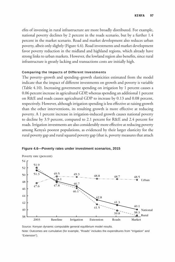
KENYA 97
efi ts of investing in rural infrastructure are more broadly distributed. For example, national poverty declines by 2 percent in the roads scenario, but by a further 1.4 percent in the market scenario. Road and market development also reduces urban poverty, albeit only slightly (Figure 4.6). Road investments and market development favor poverty reduction in the midland and highland regions, which already have strong links to urban markets. However, the lowland region also benefi ts, since rural infrastructure is greatly lacking and transactions costs are initially high.
Comparing the Impacts of Different Investments The poverty–growth and spending–growth elasticities estimated from the model indicate that the impact of different investments on growth and poverty is variable (Table 4.10). Increasing government spending on irrigation by 1 percent causes a 0.06 percent increase in agricultural GDP, whereas spending an additional 1 percent on R&E and roads causes agricultural GDP to increase by 0.13 and 0.08 percent, respectively. However, although irrigation spending is less effective at raising growth than the other interventions, its resulting growth is more effective at reducing poverty. A 1 percent increase in irrigation-induced growth causes national poverty to decline by 3.9 percent, compared to 2.1 percent for R&E and 2.4 percent for roads. Irrigation investments are also considerably more effective at reducing poverty among Kenya’s poorest populations, as evidenced by their larger elasticity for the rural poverty gap and rural squared poverty gap (that is, poverty measures that attach
Poverty rate (percent)
54
38 Rural
National
Urban
40
42
44
46
48
50
52
MarketRoadsExtensionIrrigationBaseline2003
47.6
51.3
51.9
47.8
48.1
49.5
46.1
46.7
49.3
41.5
42.8
48.8
39.8
41.3
48.7
38.3
40.1
48.5
Figure 4.6—Poverty rates under investment scenarios, 2015
Source: Kenyan dynamic computable general equilibrium model results.Note: Outcomes are cumulative (for example, “Roads” includes the expenditures from “Irrigation” and “Extension”).
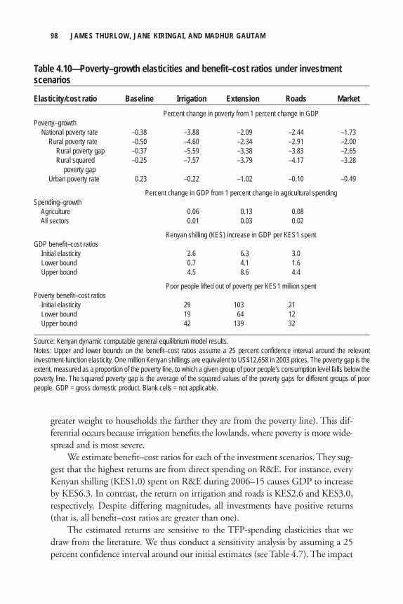
98 JAMES THURLOW, JANE KIRINGAI, AND MADHUR GAUTAM
greater weight to households the farther they are from the poverty line). This dif-ferential occurs because irrigation benefi ts the lowlands, where poverty is more wide-spread and is most severe.
We estimate benefi t–cost ratios for each of the investment scenarios. They sug-gest that the highest returns are from direct spending on R&E. For instance, every Kenyan shilling (KES1.0) spent on R&E during 2006–15 causes GDP to increase by KES6.3. In contrast, the return on irrigation and roads is KES2.6 and KES3.0, respectively. Despite differing magnitudes, all investments have positive returns (that is, all benefi t–cost ratios are greater than one).
The estimated returns are sensitive to the TFP-spending elasticities that we draw from the literature. We thus conduct a sensitivity analysis by assuming a 25 percent confi dence interval around our initial estimates (see Table 4.7). The impact
Table 4.10—Poverty–growth elasticities and benefit–cost ratios under investment scenarios
Elasticity/cost ratio Baseline Irrigation Extension Roads Market Percent change in poverty from 1 percent change in GDPPoverty–growth National poverty rate –0.38 –3.88 –2.09 –2.44 –1.73 Rural poverty rate –0.50 –4.60 –2.34 –2.91 –2.00 Rural poverty gap –0.37 –5.59 –3.38 –3.83 –2.65 Rural squared –0.25 –7.57 –3.79 –4.17 –3.28 poverty gap Urban poverty rate 0.23 –0.22 –1.02 –0.10 –0.49
Percent change in GDP from 1 percent change in agricultural spendingSpending–growth Agriculture 0.06 0.13 0.08 All sectors 0.01 0.03 0.02
Kenyan shilling (KES) increase in GDP per KES1 spentGDP benefit–cost ratios Initial elasticity 2.6 6.3 3.0 Lower bound 0.7 4.1 1.6 Upper bound 4.5 8.6 4.4
Poor people lifted out of poverty per KES1 million spentPoverty benefit–cost ratios Initial elasticity 29 103 21 Lower bound 19 64 12 Upper bound 42 139 32
Source: Kenyan dynamic computable general equilibrium model results.Notes: Upper and lower bounds on the benefit–cost ratios assume a 25 percent confidence interval around the relevant investment-function elasticity. One million Kenyan shillings are equivalent to US$12,658 in 2003 prices. The poverty gap is the extent, measured as a proportion of the poverty line, to which a given group of poor people’s consumption level falls below the poverty line. The squared poverty gap is the average of the squared values of the poverty gaps for different groups of poor people. GDP = gross domestic product. Blank cells = not applicable.
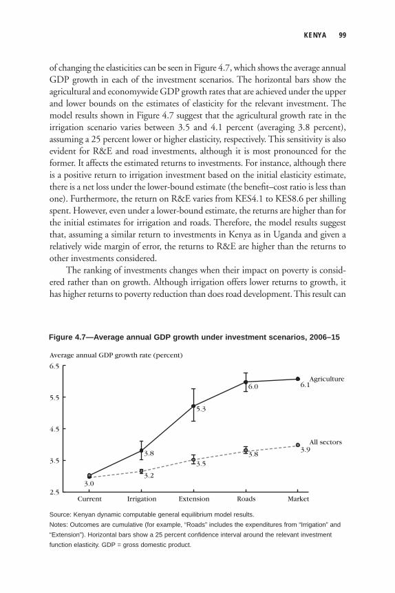
KENYA 99
of changing the elasticities can be seen in Figure 4.7, which shows the average annual GDP growth in each of the investment scenarios. The horizontal bars show the agricultural and economywide GDP growth rates that are achieved under the upper and lower bounds on the estimates of elasticity for the relevant investment. The model results shown in Figure 4.7 suggest that the agricultural growth rate in the irrigation scenario varies between 3.5 and 4.1 percent (averaging 3.8 percent), assuming a 25 percent lower or higher elasticity, respectively. This sensitivity is also evident for R&E and road investments, although it is most pronounced for the former. It affects the estimated returns to investments. For instance, although there is a positive return to irrigation investment based on the initial elasticity estimate, there is a net loss under the lower-bound estimate (the benefi t–cost ratio is less than one). Furthermore, the return on R&E varies from KES4.1 to KES8.6 per shilling spent. However, even under a lower-bound estimate, the returns are higher than for the initial estimates for irrigation and roads. Therefore, the model results suggest that, assuming a similar return to investments in Kenya as in Uganda and given a relatively wide margin of error, the returns to R&E are higher than the returns to other investments considered.
The ranking of investments changes when their impact on poverty is consid-ered rather than on growth. Although irrigation offers lower returns to growth, it has higher returns to poverty reduction than does road development. This result can
Average annual GDP growth rate (percent)
6.5
2.5
All sectors
Agriculture
3.5
4.5
5.5
MarketRoadsExtensionIrrigationCurrent
3.03.2
3.8
3.5
5.3
3.8
6.0
3.9
6.1
Figure 4.7—Average annual GDP growth under investment scenarios, 2006–15
Source: Kenyan dynamic computable general equilibrium model results.Notes: Outcomes are cumulative (for example, “Roads” includes the expenditures from “Irrigation” and “Extension”). Horizontal bars show a 25 percent confidence interval around the relevant investment function elasticity. GDP = gross domestic product.
100 JAMES THURLOW, JANE KIRINGAI, AND MADHUR GAUTAM
be explained by considering the differences in spending–growth and poverty–growth elasticities. The larger poverty–growth elasticity for irrigation offsets its smaller spending–growth elasticity. However, this result holds only when it is com-pared with road investments. Although R&E-induced growth is less effective in reducing poverty than irrigation-induced growth, R&E spending is considerably more effective at raising growth. It is this combination of pro-poor and pro-growth features that makes R&E better at reducing poverty. However, despite the strong results for extension services, it should be remembered that irrigation spending is more effective at reducing poverty in the lowlands, where poverty is most severe, and that roads and market development generate broad-based agricultural growth and benefi t urban consumers along with rural households.
Conclusions Our fi ndings indicate that Kenya should focus its development strategy on accelerat-ing economic growth, because in its current growth scenario, poverty will change little over the coming decade. However, under its current structure of growth, Kenya’s economy would have to grow by more than 10 percent per year if it is to meet the MDG1 by 2015. Although it is clear that no single sector can lead develop-ment on its own, Kenya has to search for a growth option that is more pro-poor. Our fi ndings indicate that without agricultural growth, it is unlikely that signifi cant declines in poverty can be achieved.
The need for broad-based growth also applies to subsectors in agriculture. Despite differences across agricultural sectors, agriculture typically generates growth that is more benefi cial to a majority of Kenyans. Agricultural growth is especially benefi cial for poorer households in less-favored regions. Therefore, it is unlikely that the current strategy, which is not optimistic about agriculture’s growth potential, can have a profound effect on poverty. Furthermore, an industry-led growth strategy that does not also increase investments in agriculture will exacerbate Kenya’s already high levels of income inequality. Even in urban areas, the gap between formal and informal sectors means that industrial policies geared toward the formal sector are unlikely to benefi t the urban poor in large numbers. Therefore, we conclude that, as Kenya prepares future national strategies, the country should direct greater emphasis and resources toward accelerating agricultural growth.
We have explored how agricultural growth can be accelerated through increas-ing public spending on agriculture and the rural sector. We fi nd that increasing agricultural spending to meet the 10 percent target set by the Maputo Declaration can lift an additional 1.5 million people above the poverty line by 2015. Irrigation and R&E greatly accelerate growth for both food and export crops and benefi t households throughout the country. Specifi c investments have higher returns in
KENYA 101
different parts of the country. Irrigation investments favor the lowlands and Kenya’s poorest populations, whereas R&E favors the midlands and highlands. R&E is found to have the highest returns in terms of both growth and poverty reduction. However, the reduction in poverty resulting from meeting the 10 percent agricul-tural spending target is only one-third of the reduction required to meet the MDG1. Furthermore, increasing agricultural spending to 10 percent of total spending is insuffi cient to meet the CAADP agricultural growth target of 6 percent. Achieving this target will require additional nonagricultural investments, such as improved rural infrastructure and rural market development. Even though building rural roads and reducing transaction costs is an expensive option, we fi nd that these investments signifi cantly reduce rural poverty and encourage growth that extends beyond rural areas.
The total cost of increasing agricultural and rural investments to achieve the 6 percent CAADP growth target is about US$127 million per year during 2006–15 in 2003 prices. The additional spending above the 10 percent committed to under the Maputo Declaration is US$54.9 million. However, improving the effi ciency of government investments could reduce these cost estimates. We have shown that even slight improvements in the relationship between investment and productivity can greatly improve growth and poverty outcomes. Therefore, although it is neces-sary to increase spending on agriculture, the fi scal burden of an agricultural growth strategy can be reduced through better fi scal management and implementation. Finally, we fi nd that even though the 10 percent agricultural growth target set under the CAADP initiative will cause a signifi cant decline in poverty, it still falls far short of halving poverty by 2015. Therefore, agricultural growth should be afforded a more central role in Kenya’s development strategy, but it will also be necessary to continue to encourage urban and nonagricultural growth. However, Kenya’s devel-opment strategy will have to move beyond its current overemphasis on industrializa-tion if the benefi ts of future growth are to be shared throughout the population.
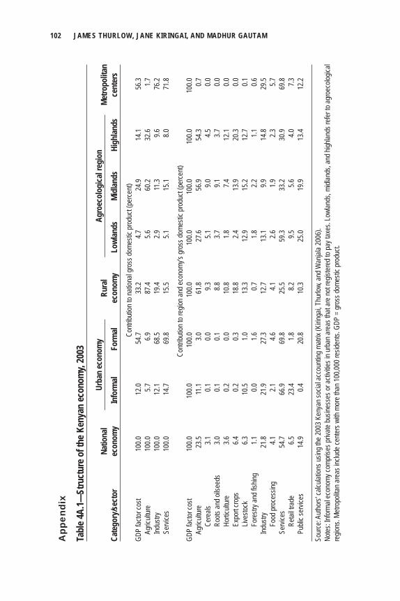
102 JAMES THURLOW, JANE KIRINGAI, AND MADHUR GAUTAM
Tabl
e 4A.
1—St
ruct
ure o
f the
Ken
yan
econ
omy,
2003
Na
tiona
l
Ru
ral
Me
tropo
litan
Cate
gory
/sect
or
econ
omy
Info
rmal
Form
al
econ
omy
Lowl
ands
Mi
dlan
ds
High
lands
ce
nter
s
Contr
ibutio
n to n
ation
al gr
oss d
omes
tic pr
oduc
t (pe
rcent)
GDP
factor
cost
100.0
12
.0 54
.7 33
.2 4.7
24
.9 14
.1 56
.3
Agric
ultur
e 10
0.0
5.7
6.9
87.4
5.6
60.2
32.6
1.7
Indus
try
100.0
12
.1 68
.5 19
.4 2.9
11
.3 9.6
76
.2
Servi
ces
100.0
14
.7 69
.8 15
.5 5.1
15
.1 8.0
71
.8
Co
ntribu
tion t
o reg
ion an
d eco
nomy
’s gr
oss d
omes
tic pr
oduc
t (pe
rcent)
GDP
factor
cost
100.0
10
0.0
100.0
10
0.0
100.0
10
0.0
100.0
10
0.0
Agric
ultur
e 23
.5 11
.1 3.0
61
.8 27
.6 56
.9 54
.3 0.7
Cere
als
3.1
0.1
0.0
9.3
5.1
9.0
4.5
0.0
Ro
ots an
d oils
eeds
3.0
0.1
0.1
8.8
3.7
9.1
3.7
0.0
Hortic
ultur
e 3.6
0.2
0.0
10
.8 1.8
7.4
12
.1 0.0
Expo
rt cro
ps
6.4
0.2
0.3
18.8
2.4
13.9
20.3
0.0
Liv
estoc
k 6.3
10
.5 1.0
13
.3 12
.9 15
.2 12
.7 0.1
Fore
stry a
nd fis
hing
1.1
0.0
1.6
0.7
1.8
2.2
1.1
0.6
Indus
try
21.8
21.9
27.3
12.7
13.1
9.9
14.8
29.5
Food
proc
essin
g 4.1
2.1
4.6
4.1
2.6
1.9
2.3
5.7
Se
rvice
s 54
.7 66
.9 69
.8 25
.5 59
.3 33
.2 30
.9 69
.8
Re
tail tr
ade
6.5
23.4
1.8
8.2
9.5
5.6
4.0
7.3
Publi
c ser
vices
14
.9 0.4
20
.8 10
.3 25
.0 19
.9 13
.4 12
.2
Sour
ce: A
uthor
s’ ca
lculat
ions u
sing t
he 20
03 K
enya
n soc
ial ac
coun
ting m
atrix
(Kirin
gai, T
hurlo
w, an
d Wan
jala 2
006)
.No
tes: In
forma
l eco
nomy
comp
rises
priva
te bu
sines
ses o
r acti
vities
in ur
ban a
reas
that
are n
ot re
gister
ed to
pay t
axes
. Low
lands
, midl
ands
, and
high
lands
refer
to ag
roec
ologic
al re
gions
. Metr
opoli
tan ar
eas i
nclud
e cen
ters w
ith m
ore t
han 1
00,00
0 res
idents
. GDP
= gr
oss d
omes
tic pr
oduc
t.
Agro
ecol
ogica
l reg
ion
Urba
n ec
onom
y
App
endi
x
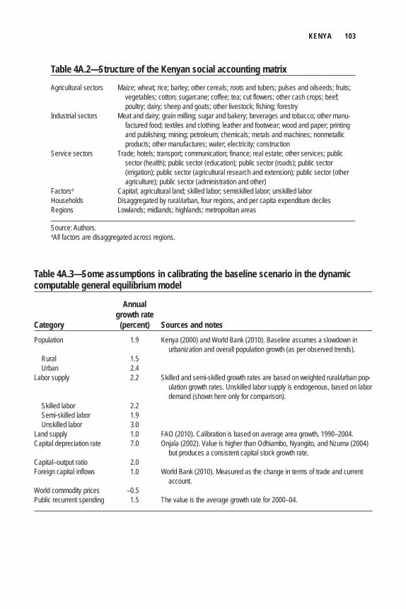
KENYA 103
Table 4A.2—Structure of the Kenyan social accounting matrix
Agricultural sectors Maize; wheat; rice; barley; other cereals; roots and tubers; pulses and oilseeds; fruits; vegetables; cotton; sugarcane; coffee; tea; cut flowers; other cash crops; beef;
poultry; dairy; sheep and goats; other livestock; fishing; forestryIndustrial sectors Meat and dairy; grain milling; sugar and bakery; beverages and tobacco; other manu- factured food; textiles and clothing; leather and footwear; wood and paper; printing
and publishing; mining; petroleum; chemicals; metals and machines; nonmetallic products; other manufactures; water; electricity; construction
Service sectors Trade; hotels; transport; communication; finance; real estate; other services; public sector (health); public sector (education); public sector (roads); public sector
(irrigation); public sector (agricultural research and extension); public sector (other agriculture); public sector (administration and other)
Factorsa Capital; agricultural land; skilled labor; semiskilled labor; unskilled laborHouseholds Disaggregated by rural/urban, four regions, and per capita expenditure decilesRegions Lowlands; midlands; highlands; metropolitan areas
Source: Authors.aAll factors are disaggregated across regions.
Table 4A.3—Some assumptions in calibrating the baseline scenario in the dynamic computable general equilibrium model
Annual growth rateCategory (percent) Sources and notesPopulation 1.9 Kenya (2000) and World Bank (2010). Baseline assumes a slowdown in urbanization and overall population growth (as per observed trends). Rural 1.5 Urban 2.4 Labor supply 2.2 Skilled and semi-skilled growth rates are based on weighted rural/urban pop- ulation growth rates. Unskilled labor supply is endogenous, based on labor
demand (shown here only for comparison). Skilled labor 2.2 Semi-skilled labor 1.9 Unskilled labor 3.0 Land supply 1.0 FAO (2010). Calibration is based on average area growth, 1990–2004. Capital depreciation rate 7.0 Onjala (2002). Value is higher than Odhiambo, Nyangito, and Nzuma (2004) but produces a consistent capital stock growth rate.Capital–output ratio 2.0 Foreign capital inflows 1.0 World Bank (2010). Measured as the change in terms of trade and current account.World commodity prices –0.5 Public recurrent spending 1.5 The value is the average growth rate for 2000–04.
104 JAMES THURLOW, JANE KIRINGAI, AND MADHUR GAUTAM
ReferencesAkroyd, S., and L. Smith. 2007. Review of Public Spending to Agriculture. Report prepared by Oxford
Policy Management. London: Department for International Development.
Ariga, J., T. S. Jayne, and J. Nyoro. 2006. Factors Driving the Growth in Fertilizer Consumption in Kenya,
1990–2005: Sustaining the Momentum in Kenya and Lessons for Broader Replicability in Sub-
Saharan Africa. Nairobi, Kenya: Tegemeo Institute of Agricultural Policy and Development,
Kenya Agricultural Research Institute.
Ekbom, A. 1998. “Some Determinants to Agricultural Productivity—An Application to Kenyan
Highlands.” Paper presented at the World Conference on Environmental Economics, Venice,
Italy, June 25–27.
Evenson, R. E., and G. Mwabu. 1998. The Effects of Agricultural Extension on Farm Yields in Kenya.
Discussion Paper 708. New Haven, CN, US: Economic Growth Center, Yale University.
Fan, S., and N. Rao. 2003. Public Spending in Developing Countries: Trend, Determination, and Impact.
Environment and Production Technology Division Discussion Paper 99. Washington, DC:
International Food Policy Research Institute.
Fan, S., and X. Zhang. 2008. “Public Expenditure, Growth, and Poverty Reduction in Rural Uganda.
Development.” African Development Review 20 (3): 466–496.
FAO (Food and Agriculture Organization of the United Nations). 2010. FAOSTAT statistical database.
Accessed September 16, 2011. http://faostat.fao.org/.
Gautam, M., and J. Anderson. 1998. Returns to T&V Extension in Kenya: Some Alternative Findings.
Africa Technical Department Series Technical Paper 208. Washington, DC: World Bank.
IMF (International Monetary Fund). Various years. Government Finance Statistics. Washington, DC.
Kabubo-Mariara, J. 2001. “Herders Response to Acute Land Pressure and Determinants of Poverty
under Changing Property Rights: Some Insights from Kenya.” Unpublished working paper,
Department of Economics, University of Nairobi, Nairobi, Kenya.
Karanja, A. M. 2003. The Dairy Industry in Kenya: The Post-Liberalization Agenda. Nairobi, Kenya:
Tegemeo Institute of Agricultural Policy and Development, Kenya Agricultural Research
Institute.
Karanja, D. D., T. S. Jayne, and P. Strasberg. 1999. Maize Productivity and the Impact of Market
Liberalization in Kenya. Nairobi, Kenya: Tegemeo Institute of Agricultural Policy and Development,
Kenya Agricultural Research Institute.
Kenya. 2000. Poverty in Kenya: Vol. 1. Incidence and Depth of Poverty. Nairobi, Kenya: Central Bureau
of Statistics, Ministry of Planning and National Development.
———. 2002. Ninth National Development Plan. Nairobi, Kenya: Central Bureau of Statistics, Ministry
of Planning and National Development.
———. 2003a. Geographic Dimensions of Wellbeing in Kenya: Who and Where Are the Poor? Nairobi,
Kenya: Central Bureau of Statistics, Ministry of Planning and National Development.
KENYA 105
———. 2003b. Economic Recovery Strategy for Wealth and Employment Creation, 2003–2007. Nairobi,
Kenya: Ministry of Planning and National Development.
———. 2006. Economic Survey: National Accounts. Nairobi, Kenya: Central Bureau of Statistics,
Ministry of Planning and National Development.
———. 2007. Kenya Vision 2030. Nairobi, Kenya: National Economic and Social Council of Kenya,
Offi ce of the President.
Kibaara, B. 2006. Rural Financial Services in Kenya: What’s Working and Why. Nairobi, Kenya:
Tegemeo Institute of Agricultural Policy and Development, Kenya Agricultural Research
Institute.
Kimalu, P., N. Nafula, D. K. Manda, G. Mwabu, and M. S. Kimenyi. 2002. A Situational Analysis of
Poverty in Kenya. Working Paper 6. Nairobi, Kenya: Kenya Institute for Public Policy Research
and Analysis.
Kiringai, J., J. Thurlow, and B. Wanjala. 2006. A 2003 Social Accounting Matrix for Kenya. Nairobi,
Kenya: Kenya Institute for Public Policy Research and Analysis.
Mose, L. O. 1999. Maize Productivity and the Impact of Market Liberalization in Kenya. Nairobi, Kenya:
Tegemeo Institute of Agricultural Policy and Development, Kenya Agricultural Research
Institute.
Nyangito, H. O. 1999. “Agricultural Sector Performance in a Changing Policy Environment.” In
Kenya’s Strategic Policies for the 21st Century, edited by P. Kimuyu, M. Wagacha, and O. Agabi.
Nairobi, Kenya: Institute for Policy Analysis and Research.
Nyoro, J. K., and T. S. Jayne. 1999. Trends in Regional Agricultural Productivity in Kenya. Kenya
Agricultural Marketing and Policy Analysis Project. Nairobi, Kenya: Tegemeo Institute of Agricultural
Policy and Development, Kenya Agricultural Research Institute.
Nyoro, J. K., M. Wanzala, and T. Awour. 2001. Increasing Kenya’s Agricultural Competitiveness: Farm
Level Issues. Nairobi, Kenya: Tegemeo Institute of Agricultural Policy and Development, Kenya
Agricultural Research Institute.
Odhiambo, W., H. O. Nyangito, and J. Nzuma. 2004. Sources and Determinants of Agricultural Growth
and Productivity in Kenya. Discussion Paper 34. Nairobi, Kenya: Kenya Institute for Public Policy
Research and Analysis.
Onjala, J. O. 2002. Total Factor Productivity in Kenya: The Links with Trade Policy. Research Paper 118.
Nairobi, Kenya: African Economic Research Consortium.
Owuor, J. 1999. Determinants of Agricultural Productivity in Kenya. Nairobi, Kenya: Tegemeo Institute
of Agricultural Policy and Development, Kenya Agricultural Research Institute.
Ravallion, M., and S. Chen. 2003. “Measuring Pro-Poor Growth.” Economic Letters 78: 93–99.
Strasberg, P. J., T. S. Jayne, T. Yamano, J. Nyoro, D. Karanja, and J. Strauss.1999. Effects of Agricultural
Commercialization on Food Crop Input Use and Productivity in Kenya. International Development
Working Paper 11463. East Lansing, MI, US: Michigan State University.

106 JAMES THURLOW, JANE KIRINGAI, AND MADHUR GAUTAM
Thurlow, J., J. Kiringai, and M. Gautam. 2007. Rural Investment to Accelerate Growth and Poverty
Reduction in Kenya. IFPRI Discussion Paper 723. Washington, DC: International Food Policy
Research Institute.
World Bank. 2008. Kenya Poverty and Inequality Assessment: Volume I. Synthesis Report. Washington,
DC.
———. 2010. World Development Indicators. Washington, DC.
C h a p t e r 5
EthiopiaXinshen Diao, Alemayehu Seyoum Taffesse, Paul Dorosh,
James Thurlow, Alejandro Nin Pratt, and Bingxin Yu
Agriculture is perhaps the most important economic sector for sustainable development and poverty reduction in Ethiopia. More than 85 percent of the population live in rural areas and depend crucially on agriculture for
their livelihoods. The sector also accounts for more than 40 percent of national gross domestic product (GDP) and 90 percent of exports, and it provides basic needs and income to more than 90 percent of the country’s poor population. In recent years the agricultural sector has driven economic growth in the overall economy while also improving food security and reducing poverty (World Bank 2007).
Although Ethiopia remains an agrarian economy, its agricultural development has been challenged by a large and rapidly growing population combined with limited and deteriorating land resources. Agricultural growth has also fl uctuated considerably and, until recently, positive growth was rarely maintained for more than three consecutive years. There have thus been many doubts about agriculture’s potential contribution to economic growth and poverty reduction in the country. Although the role of agriculture in leading industrialization and economic transfor-mation has been debated for many years, it has remained fairly political and has not been well served by rigorous empirical evidence. As the second largest country in Africa, one of the key questions dominating the policy debate has been the con-
This chapter is based on research conducted under the project “The Economic Importance of Agriculture for Sustainable Development and Poverty Reduction,” managed by the Organization for Economic Cooperation and Development. That study was fi nanced by the Government of the Netherlands. Any errors are the responsibility of the principal authors.
108 XINSHEN DIAO ET AL.
straints that the diminishing size of farm plots is imposing on agriculture’s growth potential. Moreover, although most of the population, particularly the poor, lives in rural areas, some observers doubt whether small-scale agriculture can continue to signifi cantly reduce poverty.
Even among agriculture’s proponents debate exists about what kind of agri-cultural growth should be pursued. Should the government promote large-scale agriculture, which is perhaps more likely to adopt modern technology and thus be more productive and competitive? Alternatively, should the government focus on smallholder agriculture, which might benefi t the rural population more directly? More specifi cally, should specifi c policy supports or interventions focus on export-led agriculture targeting niche foreign markets, or should staple crops and livestock be emphasized to encourage broader-based agricultural growth? This chapter con-tributes to this ongoing debate in Ethiopia by evaluating the role of agricultural growth in future economic transformation and poverty reduction. The analysis below quantitatively measures agriculture’s economywide linkages and the impact of growth in different agricultural subsectors on poverty reduction. As with other chapters in this volume, the analysis makes use of a spatially disaggregated recursive dynamic computable general equilibrium (DCGE) model (see Chapter 2).
The chapter is structured as follows. We fi rst review Ethiopia’s national develop-ment strategies and the recent performance of its agricultural sector. We then describe the structure of the Ethiopian DCGE model and the data sources used during calibration. The model results are then presented for the baseline growth scenario and the accelerated agricultural growth scenarios. Unlike other case studies in this volume, no detailed investment analysis is done for Ethiopia. However, the fi nal section draws together our fi ndings and summarizes their implications for future national and agricultural development strategies in Ethiopia.
Agriculture in Ethiopia
Overview of Agricultural Policies and Development StrategiesAlthough Ethiopia has experienced three major political regime changes in recent history, the importance of agriculture has been recognized by each government throughout this period. However, the policies pursued by successive administrations have resulted in very different outcomes. Only over the past two decades has the country’s agricultural development strategy become more focused and policies more consistent with promoting sustainable improvements in agricultural productivity. The Derg regime (1975–1991) was characterized as an agrarian socialist regime with widespread government controls in all economic spheres, including agricul-ture. After overthrowing the imperial regime of Haile Selassie, the Derg announced
ETHIOPIA 109
an agrarian reform program in which all rural land was made the property of the state. Almost all other assets in the industrial and services sectors were national-ized, including factories, fi nancial institutions, large hotels, and many residential buildings.
The agrarian reform prohibited all tenancy relations and provided a large num-ber of rural households with access to land for cultivation. However, restrictions on plot size per family, prohibition of hired agricultural labor, intensifi cation of col-lectivization, establishment of large-scale state farms, and a series of other antimarket and state-controlled economic instruments created negative incentives for farmers and distorted market mechanisms guiding land allocation and productivity improve-ments. Although this central planning development strategy identifi ed agriculture as a key engine of growth and targeted improved food security and agricultural productivity, most of these targets remained on paper, and few were achieved. As a result, the economy was approaching a macroeconomic crisis by the end of the Derg regime—a fact that was compounded by the onset of Ethiopia’s worst famine on record in 1984.
Weak policies and political repression during the Derg period not only gener-ated disastrous economic outcomes but also led to civil confl ict. The Derg regime collapsed in 1991, and the Ethiopian People’s Revolutionary Democratic Front (EPRDF) assumed power. The years that followed witnessed a radical shift in gov-ernment policy. Both the transitional government (1991–94) and the EPRDF government initiated extensive economic reforms, including market liberalization and a structural adjustment program. At the macro level, import protection was reduced, foreign exchange controls were eased, and state-owned enterprises were privatized, including banks. In agriculture, cooperative membership was made compulsory, grain delivery was discontinued, and fertilizers subsidies were discon-tinued. Consequently, the direct role of the state in economic activity declined dramatically.
The most important development strategy that emerged under the transitional government was the adoption of Agriculture Development Led Industrialization (ADLI), which has remained a central component of the current government’s development program until recent years. ADLI focuses on the productivity growth of small farms and on labor-intensive industrialization. This strategy has been justi-fi ed by agriculture’s large contribution to national income, employment, and exports, and by the gaps between rural and urban incomes.
Consistent with ADLI, in the mid-1990s, the government refocused its policy reforms from market-based mechanisms (“getting the prices right”) to more active public investment in agricultural extension aimed at boosting productivity through the widespread introduction of modern technology (MOFED 2002). An extensive extension program—the Participatory Demonstration and Training Extension
110 XINSHEN DIAO ET AL.
System (PADETES)—was implemented, and through this system, the government delivered off-the-shelf packages of fertilizer, improved seed, and credit, as well as information on input use and better agricultural practices to most rural small-holders. The promotion of the credit–fertilizer package was accompanied by further liberalization of fertilizer markets. By 1997, fertilizer subsidies were completely removed, and retail prices were fully liberalized, which also resulted in higher fertil-izer prices. Fertilizer use increased, although diffusion and adoption rates remained disappointing, despite the vigorous promotion of the credit–fertilizer packages. Overall, agricultural output continued to fall behind population growth.
Acknowledging the limited success of PADETES, the government revisited the program and formulated an integrated rural and agriculture development strategy that was launched in 2002. The new strategy—offi cially known as the Sustainable Development and Poverty Reduction Program (SDPRP)—centered on the goal of poverty reduction (MOFED 2002). In line with SDPRP, the government intro-duced fi scal decentralization, judicial and civil service reform, and public sector capacity building. After the continuing evidence of widespread food insecurity dur-ing the drought of 2002/03, the government also implemented social safety nets, programs to build the assets of food-insecure households, land resettlement, and soil and water conservation (especially water harvesting).
The SDPRP, which covered the three years between 2002/03 and 2004/05, was the fi rst full Poverty Reduction Strategy Paper (PRSP) developed and implemented by the Ethiopian government. It was followed by the current PRSP titled “Plan for Accelerated and Sustained Development to End Poverty” (PASDEP). PASDEP formed Ethiopia’s guiding strategic framework for the fi ve-year period 2005/06–2009/10 (MOFED 2005). PASDEP aims to signifi cantly accelerate growth via the commercialization of agriculture and the promotion of private sector development. It focuses on several areas in setting its targets and designing interventions, including adopting a geographically differentiated strategy, addressing population growth, expanding and improving infrastructure, managing risk, and creating employment (MOFED 2005). The instruments to achieve these goals include farm-to-market roads, agricultural credit, extension services, national business plans tailored to specialized export crops (for example, spices, cut fl owers, fruits, and vegetables), irrigation and multipurpose dams, land tenure security and provision of land for large-scale commercial farming, and reforms to improve the availability of fertilizer and seeds.
Recent Agricultural PerformanceIn recent years policy reforms, agricultural investments, and public service provi-sions have boosted agricultural production, particularly cereals. After 2003, Ethiopian agriculture witnessed its most rapid growth period in history. As Figure 5.1 indi-
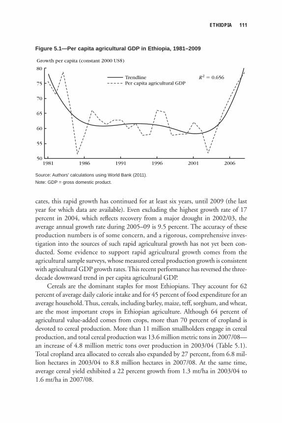
ETHIOPIA 111
cates, this rapid growth has continued for at least six years, until 2009 (the last year for which data are available). Even excluding the highest growth rate of 17 percent in 2004, which refl ects recovery from a major drought in 2002/03, the average annual growth rate during 2005–09 is 9.5 percent. The accuracy of these production numbers is of some concern, and a rigorous, comprehensive inves-tigation into the sources of such rapid agricultural growth has not yet been con-ducted. Some evidence to support rapid agricultural growth comes from the agricultural sample surveys, whose measured cereal production growth is consistent with agricultural GDP growth rates. This recent performance has reversed the three-decade downward trend in per capita agricultural GDP.
Cereals are the dominant staples for most Ethiopians. They account for 62 percent of average daily calorie intake and for 45 percent of food expenditure for an average household. Thus, cereals, including barley, maize, teff, sorghum, and wheat, are the most important crops in Ethiopian agriculture. Although 64 percent of agricultural value-added comes from crops, more than 70 percent of cropland is devoted to cereal production. More than 11 million smallholders engage in cereal production, and total cereal production was 13.6 million metric tons in 2007/08—an increase of 4.8 million metric tons over production in 2003/04 (Table 5.1). Total cropland area allocated to cereals also expanded by 27 percent, from 6.8 mil-lion hectares in 2003/04 to 8.8 million hectares in 2007/08. At the same time, average cereal yield exhibited a 22 percent growth from 1.3 mt/ha in 2003/04 to 1.6 mt/ha in 2007/08.
Growth per capita (constant 2000 US$)
80
50
65
70
55
60
75
20062001199619911981 1986
Per capita agricultural GDPTrendline R2 � 0.656
Figure 5.1—Per capita agricultural GDP in Ethiopia, 1981–2009
Source: Authors’ calculations using World Bank (2011).Note: GDP = gross domestic product.
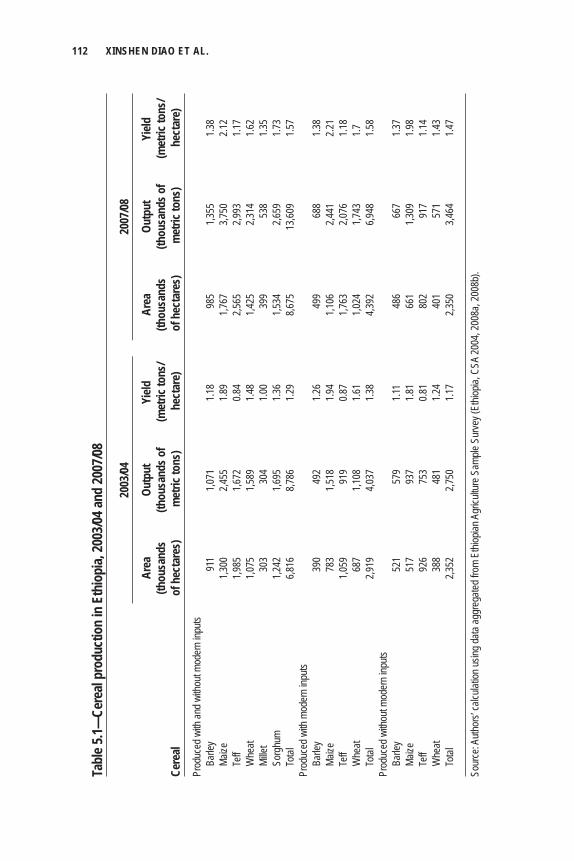
112 XINSHEN DIAO ET AL.
Tabl
e 5.1—
Cere
al pr
oduc
tion
in E
thio
pia,
2003
/04 an
d 20
07/08
20
03/04
20
07/08
Ar
ea
Outp
ut
Yield
Ar
ea
Outp
ut
Yield
(th
ousa
nds
(thou
sand
s of
(met
ric to
ns/
(thou
sand
s (th
ousa
nds o
f (m
etric
tons
/Ce
real
of h
ecta
res)
m
etric
tons
) h
ecta
re)
of h
ecta
res)
m
etric
tons
) h
ecta
re)
Prod
uced
with
and w
ithou
t mod
ern i
nputs
Ba
rley
911
1,071
1.1
8 98
5 1,3
55
1.38
Ma
ize
1,300
2,4
55
1.89
1,767
3,7
50
2.12
Te
ff 1,9
85
1,672
0.8
4 2,5
65
2,993
1.1
7
Whe
at 1,0
75
1,589
1.4
8 1,4
25
2,314
1.6
2
Mille
t 30
3 30
4 1.0
0 39
9 53
8 1.3
5
Sorg
hum
1,242
1,6
95
1.36
1,534
2,6
59
1.73
To
tal
6,816
8,7
86
1.29
8,675
13
,609
1.57
Prod
uced
with
mod
ern i
nputs
Ba
rley
390
492
1.26
499
688
1.38
Ma
ize
783
1,518
1.9
4 1,1
06
2,441
2.2
1
Teff
1,059
91
9 0.8
7 1,7
63
2,076
1.1
8
Whe
at 68
7 1,1
08
1.61
1,024
1,7
43
1.7
Total
2,9
19
4,037
1.3
8 4,3
92
6,948
1.5
8Pr
oduc
ed w
ithou
t mod
ern i
nputs
Ba
rley
521
579
1.11
486
667
1.37
Ma
ize
517
937
1.81
661
1,309
1.9
8
Teff
926
753
0.81
802
917
1.14
W
heat
388
481
1.24
401
571
1.43
To
tal
2,352
2,7
50
1.17
2,350
3,4
64
1.47
Sour
ce: A
uthor
s’ ca
lculat
ion us
ing da
ta ag
greg
ated f
rom
Ethio
pian A
gricu
lture
Sam
ple S
urve
y (Et
hiopia
, CSA
2004
, 200
8a, 2
008b
).
ETHIOPIA 113
Teff is the favored staple crop for both rural and urban consumers at all income levels and has high income elasticity of demand relative to other cereals (see Table 5A.1 in the appendix to this chapter). Not surprisingly then, more than 30 percent of total cereal land in 2007 was allocated to teff production. The next most impor-tant foodcrop is maize, which occupies 20 percent of total cereal land, followed by sorghum (18 percent), wheat (16 percent), and barley (12 percent). Although most cereal crops are used as staple foods, barley is also used for local alcohol production. In terms of volume of production in the same year (2007), maize actually ranked fi rst, with 3.8 million metric tons of output (teff is 3.0 million metric tons). Despite occupying 30 percent of cereal land, teff output is only equivalent to 22 percent of cereal output. Thus, teff is much less productive in terms of land use. Indeed, the national average yield of maize is 2.1 mt/ha in 2007, whereas teff yields are only 1.2 mt/ha—the lowest yield among all major cereal crops. Teff is only grown in a few countries, and its yield response to fertilizer is relatively limited, given that the technology needed to develop high-yield teff varieties is more diffi cult to develop than that for other cereal crops, which are more broadly grown and researched around the world. This inconsistency between the technology potential and con-sumer preference presents a potential challenge for Ethiopian food security.
Under ADLI, the government emphasized intensifi cation to increase agricul-tural production, especially through a centralized extension system to push techno-logical packages that combined credit, fertilizers, improved seeds, and better farm management practices. Under this program, fertilizer use almost doubled between 1990 and 2000 to 290,000 metric tons (World Bank 2007). However, the intensity of fertilizer nutrient use per hectare stagnated in the latter half of 1990s and the present decade. According to World Bank (2007), only 37 percent of farmers use inorganic fertilizer, and application rates remain low at 16 kg/ha of nutrients (about 33 kg/ha for commercial products).
Following the 2002/03 drought, a large-scale food security program was scaled up in poor and vulnerable areas, amounting to a signifi cant share of total public spending. More recently, weaknesses in the marketing system have been recognized, and a new marketing strategy is being developed based on scaling-up cooperatives and establishing a commodity exchange (and its associated institutions). As a result of these various programs, public spending on agriculture, natural resources, and food security increased from 5 percent of the total government budget in 1997/98 to more than 10 percent in 2003/04.
Concerted efforts to promote intensifi cation seem to be showing some positive results in recent years. Consistent with growth in total agricultural GDP, 2003/04–2007/08 registered record cereal production growth in Ethiopian history. Total cereal production increased by 54.9 percent in four years (that is, more than 10 percent per year). Against the historical trend in which almost all increased produc-
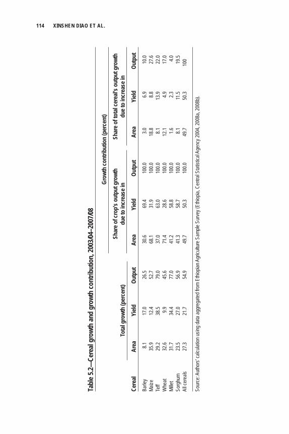
114 XINSHEN DIAO ET AL.
Tabl
e 5.2—
Cere
al gr
owth
and
grow
th co
ntrib
utio
n, 20
03/04
–200
7/08
Gr
owth
cont
ribut
ion
(per
cent
)
Sh
are o
f cro
p’s o
utpu
t gro
wth
Sh
are o
f tot
al ce
real’
s out
put g
rowt
h
due t
o in
crea
se in
du
e to
incr
ease
in
Cere
al Ar
ea
Yield
Ou
tput
Ar
ea
Yield
Ou
tput
Ar
ea
Yield
Ou
tput
Barle
y 8.1
17
.0 26
.5 30
.6 69
.4 10
0.0
3.0
6.9
10.0
Maize
35
.9 12
.4 52
.7 68
.1 31
.9 10
0.0
18.8
8.8
27.6
Teff
29.2
38.5
79.0
37.0
63.0
100.0
8.1
13
.9 22
.0W
heat
32.6
9.9
45.6
71.4
28.6
100.0
12
.1 4.9
17
.0Mi
llet
31.7
34.4
77.0
41.2
58.8
100.0
1.6
2.3
4.0
Sorg
hum
23.5
27.0
56.9
41.3
58.7
100.0
8.1
11
.5 19
.5Al
l cer
eals
27.3
21.7
54.9
49.7
50.3
100.0
49
.7 50
.3 10
0
Sour
ce: A
uthor
s’ ca
lculat
ion us
ing da
ta ag
greg
ated f
rom
Ethio
pian A
gricu
lture
Sam
ple S
urve
y (Et
hiopia
, Cen
tral S
tatist
ical A
genc
y 200
4, 20
08a,
2008
b).
Tota
l gro
wth
(per
cent
)
ETHIOPIA 115
tion was accounted for by area expansion, Table 5.2 shows that about half of recent growth has been due to yield increases. The table also presents the growth of indi-vidual crops and decomposes this into area expansion and yield increases. Among the four main cereal crops, there are two crops, teff and sorghum, for which growth in production is a dominant result of yield increases, which contributes to 63 and 58.7 percent of teff and sorghum output growth, respectively. Even though area expansion is the main source of growth for maize and wheat, increases in yields still account for 32 and 29 percent of their output growth, respectively.1
An important characteristic of Ethiopia’s agricultural sector is the high geo-graphic concentration of cereal cultivation. Almost 80 percent of total area under cereals is in the Amhara and Oromia regions (that is, northwest, west, southwest, and south of Addis Ababa). This area includes a diverse set of conditions for agri-cultural production. The spatial conditions for crop production and access to markets are characterized in Diao and Nin Pratt (2007) and Taffesse (2007).
Table 5.1 also separates production of the four main cereals by whether modern inputs are used in their production. Recently, Ethiopia has witnessed a rapid increase in modern input use, particularly fertilizer. The government’s fertilizer-promotion policy currently focuses on the four main cereal crops, which are relatively more responsive to fertilizer and have higher producer prices. Table 5.1 shows the result of this program: in 2003/04, fewer than 3 million hectares used to grow barley, maize, teff, and wheat (over 50 percent of the total area devoted to these crops) used modern inputs; by 2007/08, the area that used modern inputs had increased to more than 4 million hectares (over 60 percent of the total area devoted to these four crops). In these four years, total harvest areas of these four crops increased by 28 percent, but the areas not using modern input remained constant at about 2.3 million hectares.
Unfortunately, the observed yield difference between production with and without modern inputs is fairly modest for all four cereals crops. With the exception of wheat, the average yield when using modern inputs is less than 15 percent higher than the average yield without such inputs. Even for wheat, the yield gap was 30 percent in 2003/04 but has since fallen to 19 percent in 2007/08. Although many factors affect fertilizer effi ciency, increased use of fertilizer without use of high-yield seed varieties seems to be the most important factor. The combined use of fertilizer and improved seed is extremely low for teff and wheat farmers. Moreover, the low yield response to combined seed–fertilizer use indicates that the so-called “improved” seed are not really high-yielding varieties. Further assessment is needed to under-stand farmer’s behavior and the constraints to promoting modern input use in Ethiopia.
Agricultural performance in recent years also refl ects the new direction taken in the country’s development strategy (that is, PASDEP), which targets market-
116 XINSHEN DIAO ET AL.
driven diversifi cation and commercialization and the increase of private sector exports. After improving incentives for private investment in the fl ower industry, for example, more than 100 new investors entered the industry, and exports increased to nearly US$13 million by 2005. Other investments in high-value products and supply chains include exports of green beans to Europe and provision of higher quality milk and poultry to local urban centers. Several of these emerging industries involve outgrower or contract arrangements with small farmers, often linked to an emerging indigenous entrepreneurial class of farmers and agribusinesses. Exports of oilseeds and pulses (two traditional cash crops) have also experienced impressive growth—increasing their value by a factor of 10 between 1997 and 2006 and dem-onstrating their increasing competitiveness and the uptake of new technologies. Although coffee is still the most important export crop in Ethiopia, the combined exports of other crops and leather has sometimes surpassed the value of coffee exports in recent years.
The Ethiopian DCGE ModelWe apply the DCGE model described in Chapter 2 to assess the contribution of agricultural sectors to economywide growth and poverty reduction. The DCGE model for Ethiopia was developed by Dorosh and Thurlow (2009) based on an adapted version of the social accounting matrix developed by Ahmed et al. (2009). Given that the Ethiopian economy is still dominated by agriculture and that more than 80 percent of the population lives in the rural areas, special attention has been paid to the structure of agriculture in the model. There are 24 agricultural sectors (see Table 5A.2 in the appendix). Crop production is the most important agricultural activity, hence the model defi nes fi ve broad crop groups:
1. Cereal crops, which are separated into teff, barley, wheat, maize, and sorghum and millet.
2. Pulses and oilseeds, both of which are aggregated crop groups in the model. In Ethiopia, the most important oilseed crops are sesame and groundnuts.
3. Horticulture, which is separated into fruits, vegetables, and enset.
4. High-value export-oriented crops, which are separated into coffee, cotton, cut fl owers, sugarcane, tea, and tobacco.
5. Other crops, including chat and root crops.
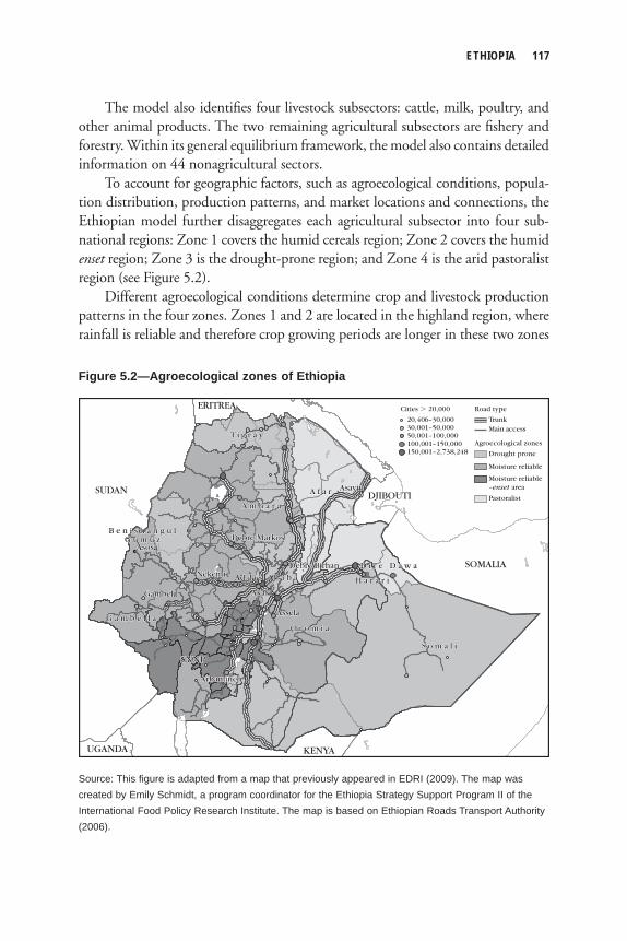
ETHIOPIA 117
The model also identifi es four livestock subsectors: cattle, milk, poultry, and other animal products. The two remaining agricultural subsectors are fi shery and forestry. Within its general equilibrium framework, the model also contains detailed information on 44 nonagricultural sectors.
To account for geographic factors, such as agroecological conditions, popula-tion distribution, production patterns, and market locations and connections, the Ethiopian model further disaggregates each agricultural subsector into four sub-national regions: Zone 1 covers the humid cereals region; Zone 2 covers the humid enset region; Zone 3 is the drought-prone region; and Zone 4 is the arid pastoralist region (see Figure 5.2).
Different agroecological conditions determine crop and livestock production patterns in the four zones. Zones 1 and 2 are located in the highland region, where rainfall is reliable and therefore crop growing periods are longer in these two zones
SUDANSUDAN
SOMALIASOMALIA
KENYAKENYA
ERITREAERITREA
DJIBOUTIDJIBOUTI
UGANDAUGANDA
AsAsososa
GambelGambela
AsAsayayitita
S o m a l iS o m a l i
O r o m i aO r o m i a
A f a rA f a r
A m h a r aA m h a r a
SNNPSNNP
T iT i g r ag r a y
G a m b e l l aG a m b e l l a
B e n i s h a n g u lB e n i s h a n g u lG u m u zG u m u z
D iD i r er e D a w D a w a
H a r a r iH a r a r iAd d id d i s s Ab a b ab a b a
ArArbaminbaminchch
DeDebrbre e BirBirhanhan
DeDebrbre e MaMarkosrkos
NeNekekemtmte
AsAsseselala
AkAkakaki
SUDAN
SOMALIA
KENYA
ERITREA
DJIBOUTI
UGANDA
Asosa
Gambela
Asayita
S o m a l i
O r o m i a
A f a r
A m h a r a
SNNP
T i g r a y
G a m b e l l a
B e n i s h a n g u lG u m u z
D i r e D a w a
H a r a r iAd d i s Ab a b a
Cities � 20,000
20,406–30,00030,001–50,00050,001–100,000100,001–150,000150,001–2,738,248
Road type
TrunkMain access
Agroecological zones
Drought prone
Moisture reliable
Moisture reliable–enset area
Pastoralist
Arbaminch
Debre Birhan
Debre Markos
Nekemte
Assela
Akaki
Figure 5.2—Agroecological zones of Ethiopia
Source: This figure is adapted from a map that previously appeared in EDRI (2009). The map was created by Emily Schmidt, a program coordinator for the Ethiopia Strategy Support Program II of the International Food Policy Research Institute. The map is based on Ethiopian Roads Transport Authority (2006).
118 XINSHEN DIAO ET AL.
than elsewhere. Because Ethiopia’s agriculture is mainly rainfed, suitable rainfall conditions explain why these two zones have high agricultural potential. In fact, Zone 1 is the country’s grain basket: it produces 60–70 percent of the country’s cereals. Although Zone 3 is larger than Zone 1, it has less reliable rainfall and so only produces 25–30 percent of total production for most grain crops. The excep-tions are sorghum and millet, which are relatively drought resistant. Hence, Zone 3 produces about 50 percent of these crops. Zone 4 is called a “pastoralist region,” but only about one-fi fth of national livestock is produced in this zone because of harsh agroecological conditions and low population densities. In contrast, more than 40 percent of livestock is produced in Zone 1, refl ecting the close relationship between crops and livestock production among smallholders in Ethiopia.
The household structure in the DCGE model allows us to conduct growth–poverty linkage analysis. In the model, there are 12 representative household groups that are disaggregated by the four rural zones, small and large urban centers, and income level (poor or nonpoor status). “Poor” is defi ned as all households falling into the lowest two per capita expenditure quintiles (that is, the poorest 40 percent of the population defi ned at the national level). Household income elasticities are based on estimates from the 2004/05 Household Income and Expenditure Survey (HICES) (Ethiopia, CSA 2005; see Table 5A.1 in the appendix). Each household questioned in HICES 2004/05 is linked directly to the corresponding representative household in the model through a top-down consumption-based microsimulation model (see Chapter 2). In this formulation of the model, changes in representative households’ consumption and prices in the DCGE model are passed down to the survey, where total real consumption for each survey household is recalculated. This new level of per capita total consumption for each survey household is compared to a poverty line, so that poverty headcount can be recalculated.
Both total and sector GDPs are endogenous variables, and their growth comes from three major dynamic factors incorporated in the model: (1) growth in factor supply, (2) change in total factor productivity (TFP), and (3) accumulation of capi-tal through investment. By design, the supplies of skilled and unskilled labor, agri-cultural land, and livestock stocks are fi xed in each time period, and annual growth rates are exogenously imposed. In contrast, the supply of agriculture-specifi c labor (that is, family workers) and workers with elementary occupations are fl exible (that is, they are endogenous) and depend on supply elasticities with respect to wage rates, which endogenously change over time. Changes in TFP at the subsector level are exogenous, whereas capital accumulation as an endogenous variable is the out-come of past investment, which is fi nanced by private, public, and foreign savings. Foreign savings is an exogenous variable chosen as a macroclosure to balance the foreign account in the model. Public savings is a residual term between government
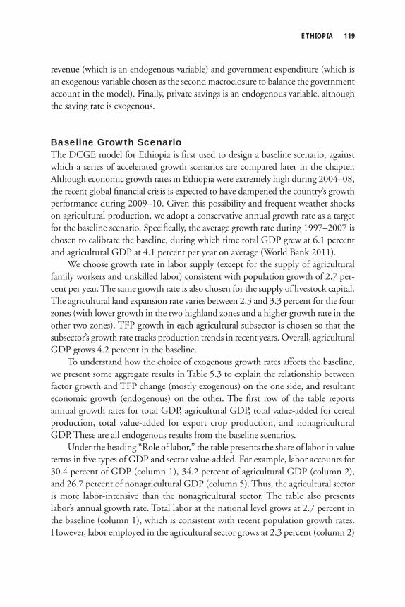
ETHIOPIA 119
revenue (which is an endogenous variable) and government expenditure (which is an exogenous variable chosen as the second macroclosure to balance the government account in the model). Finally, private savings is an endogenous variable, although the saving rate is exogenous.
Baseline Growth Scenario The DCGE model for Ethiopia is fi rst used to design a baseline scenario, against which a series of accelerated growth scenarios are compared later in the chapter. Although economic growth rates in Ethiopia were extremely high during 2004–08, the recent global fi nancial crisis is expected to have dampened the country’s growth performance during 2009–10. Given this possibility and frequent weather shocks on agricultural production, we adopt a conservative annual growth rate as a target for the baseline scenario. Specifi cally, the average growth rate during 1997–2007 is chosen to calibrate the baseline, during which time total GDP grew at 6.1 percent and agricultural GDP at 4.1 percent per year on average (World Bank 2011).
We choose growth rate in labor supply (except for the supply of agricultural family workers and unskilled labor) consistent with population growth of 2.7 per-cent per year. The same growth rate is also chosen for the supply of livestock capital. The agricultural land expansion rate varies between 2.3 and 3.3 percent for the four zones (with lower growth in the two highland zones and a higher growth rate in the other two zones). TFP growth in each agricultural subsector is chosen so that the subsector’s growth rate tracks production trends in recent years. Overall, agricultural GDP grows 4.2 percent in the baseline.
To understand how the choice of exogenous growth rates affects the baseline, we present some aggregate results in Table 5.3 to explain the relationship between factor growth and TFP change (mostly exogenous) on the one side, and resultant economic growth (endogenous) on the other. The fi rst row of the table reports annual growth rates for total GDP, agricultural GDP, total value-added for cereal production, total value-added for export crop production, and nonagricultural GDP. These are all endogenous results from the baseline scenarios.
Under the heading “Role of labor,” the table presents the share of labor in value terms in fi ve types of GDP and sector value-added. For example, labor accounts for 30.4 percent of GDP (column 1), 34.2 percent of agricultural GDP (column 2), and 26.7 percent of nonagricultural GDP (column 5). Thus, the agricultural sector is more labor-intensive than the nonagricultural sector. The table also presents labor’s annual growth rate. Total labor at the national level grows at 2.7 percent in the baseline (column 1), which is consistent with recent population growth rates. However, labor employed in the agricultural sector grows at 2.3 percent (column 2)
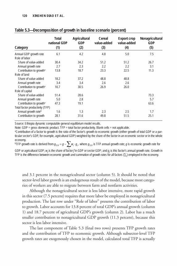
120 XINSHEN DIAO ET AL.
and 3.1 percent in the nonagricultural sector (column 5). It should be noted that sector-level labor growth is an endogenous result of the model, because most catego-ries of workers are able to migrate between farm and nonfarm activities.
Although the nonagricultural sector is less labor intensive, more rapid growth in this sector (7.5 percent) requires that more labor be employed in nonagricultural production. The last row under “Role of labor” presents the contribution of labor to growth. Labor accounts for 13.8 percent of total GDP’s annual growth (column 1) and 18.7 percent of agricultural GDP’s growth (column 2). Labor has a much smaller contribution to nonagricultural GDP growth (11.3 percent), because this sector is less labor intensive.
The last component of Table 5.3 (fi nal two rows) presents TFP growth rates and the contribution of TFP to economic growth. Although subsector-level TFP growth rates are exogenously chosen in the model, calculated total TFP is actually
Table 5.3—Decomposition of growth in baseline scenario (percent)
Total Agricultural Cereal Export crop Nonagricultural national GDP GDP value-added value-added GDPCategory (1) (2) (3) (4) (5)Annual GDP growth rate 6.1 4.2 4.8 5.0 7.5Role of labor Share of value-added 30.4 34.2 51.2 51.2 26.7 Annual growth rate 2.7 2.3 2.2 2.2 3.1 Contribution to growtha 13.8 18.7 23.3 22.5 11.3Role of land Share of value-added 18.2 37.2 48.8 48.8 Annual growth rate 3.4 3.4 2.6 2.6 Contribution to growtha 10.7 30.5 26.9 26.0 Role of capital Share of value-added 51.4 28.6 73.3 Annual growth rate 5.0 2.8 5.7 Contribution to growtha 47.3 19.1 63.6Total factor productivity (TFP) Annual growth rateb 1.6 1.3 2.3 2.5 1.7 Contribution to growth 28.1 31.6 49.8 51.5 25.1
Source: Ethiopia dynamic computable general equilibrium model results.Note: GDP = gross domestic product. TFP = total factor productivity. Blank cells = not applicable.aContribution of a factor to growth is the ratio of the factor’s growth to economic growth (either growth of total GDP or a par-ticular sector’s GDP, for example, agricultural GDP) weighted by the share of the factor in an economic sector or in the whole economy.bTFP growth rate is derived from gTFP = g – ∑wt gt , where gTFP is TFP annual growth rate; g is economic growth rate for tGDP or agricultural GDP; wf is the share of factor f in GDP or sector GDP; and gf is this factor’s annual growth rate. Growth in TFP is the difference between economic growth and summation of growth rates for all factors (∑t) employed in the economy.
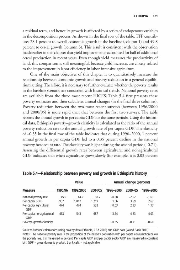
ETHIOPIA 121
a residual term, and hence its growth is affected by a series of endogenous variables in the decomposition process. As shown in the fi nal row of the table, TFP contrib-utes 28.1 percent to overall economic growth in the baseline (column 1) and 49.8 percent to cereal growth (column 3). This result is consistent with the observation made earlier in this chapter that yield improvements accounted for half of additional cereal production in recent years. Even though yield measures the productivity of land, this comparison is still meaningful, because yield increases are closely related to the improvement in labor effi ciency in labor-intensive agriculture.
One of the main objectives of this chapter is to quantitatively measure the relationship between economic growth and poverty reduction in a general equilib-rium setting. Therefore, it is necessary to further evaluate whether the poverty results in the baseline scenario are consistent with historical trends. National poverty rates are available from the three most recent HICES. Table 5.4 fi rst presents these poverty estimates and then calculates annual changes (in the fi nal three columns). Poverty reduction between the two most recent surveys (between 1996/2000 and 2000/05) is more rapid than that between the fi rst two surveys. The table reports the annual growth in per capita GDP for the same periods. Using the histori-cal data, Ethiopia’s poverty–growth elasticity is calculated as the ratio of the annual poverty reduction rate to the annual growth rate of per capita GDP. The elasticity of –0.35 in the fi nal row of the table indicates that during 1996–2000, 1 percent annual growth in per capita GDP led to a 0.35 percent decline in the national poverty headcount rate. The elasticity was higher during the second period (–0.71). Assessing the differential growth rates between agricultural and nonagricultural GDP indicates that when agriculture grows slowly (for example, it is 0.03 percent
Table 5.4—Relationship between poverty and growth in Ethiopia’s history
Value Annual change (percent)
Measure 1995/96 1999/2000 2004/05 1996–2000 2000–05 1996–2005National poverty rate 45.5 44.2 38.7 –0.58 –2.62 –1.61Per capita GDP 937 1,017 1,219 1.66 3.69 2.67Per capita agricultural 474 474 532 0.03 2.33 1.17 GDP Per capita nonagricultural 463 543 687 3.24 4.83 4.03 GDP Poverty–growth elasticity –0.35 –0.71 –0.60
Source: Authors’ calculations using poverty data (Ethiopia, CSA 2005) and GDP data (World Bank 2011).Notes: The national poverty rate is the proportion of the nation’s population with per capita consumption below the poverty line. It is measured in percent. Per capita GDP and per capita sector GDP are measured in constant birr. GDP = gross domestic product. Blank cells = not applicable.
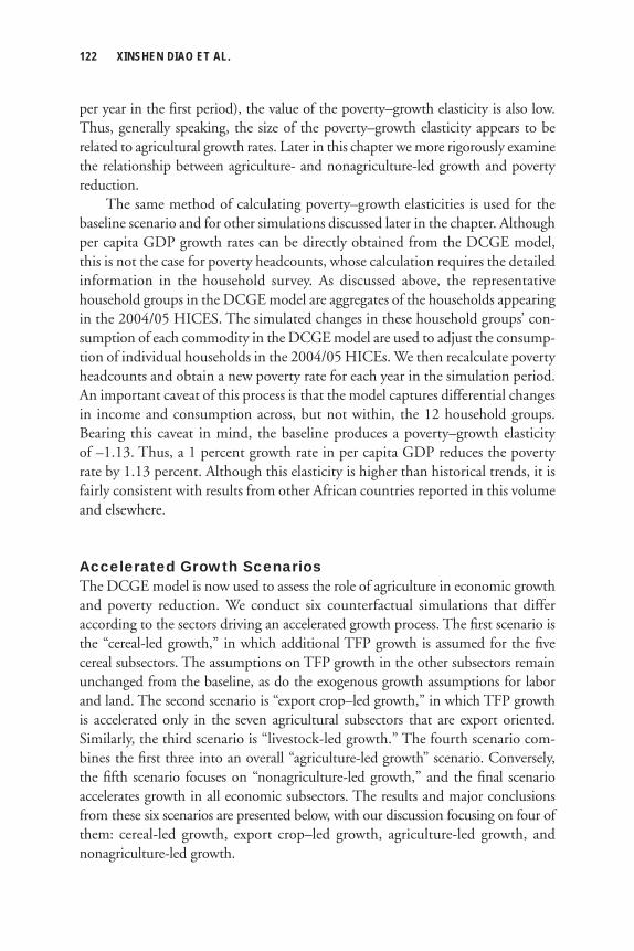
122 XINSHEN DIAO ET AL.
per year in the fi rst period), the value of the poverty–growth elasticity is also low. Thus, generally speaking, the size of the poverty–growth elasticity appears to be related to agricultural growth rates. Later in this chapter we more rigorously examine the relationship between agriculture- and nonagriculture-led growth and poverty reduction.
The same method of calculating poverty–growth elasticities is used for the baseline scenario and for other simulations discussed later in the chapter. Although per capita GDP growth rates can be directly obtained from the DCGE model, this is not the case for poverty headcounts, whose calculation requires the detailed information in the household survey. As discussed above, the representative household groups in the DCGE model are aggregates of the households appearing in the 2004/05 HICES. The simulated changes in these household groups’ con-sumption of each commodity in the DCGE model are used to adjust the consump-tion of individual households in the 2004/05 HICEs. We then recalculate poverty headcounts and obtain a new poverty rate for each year in the simulation period. An important caveat of this process is that the model captures differential changes in income and consumption across, but not within, the 12 household groups. Bearing this caveat in mind, the baseline produces a poverty–growth elasticity of –1.13. Thus, a 1 percent growth rate in per capita GDP reduces the poverty rate by 1.13 percent. Although this elasticity is higher than historical trends, it is fairly consistent with results from other African countries reported in this volume and elsewhere.
Accelerated Growth Scenarios The DCGE model is now used to assess the role of agriculture in economic growth and poverty reduction. We conduct six counterfactual simulations that differ according to the sectors driving an accelerated growth process. The fi rst scenario is the “cereal-led growth,” in which additional TFP growth is assumed for the fi ve cereal subsectors. The assumptions on TFP growth in the other subsectors remain unchanged from the baseline, as do the exogenous growth assumptions for labor and land. The second scenario is “export crop–led growth,” in which TFP growth is accelerated only in the seven agricultural subsectors that are export oriented. Similarly, the third scenario is “livestock-led growth.” The fourth scenario com-bines the fi rst three into an overall “agriculture-led growth” scenario. Conversely, the fi fth scenario focuses on “nonagriculture-led growth,” and the fi nal scenario accelerates growth in all economic subsectors. The results and major conclusions from these six scenarios are presented below, with our discussion focusing on four of them: cereal-led growth, export crop–led growth, agriculture-led growth, and nonagriculture-led growth.
ETHIOPIA 123
Subsector (Crop-Level) Growth, Employment and Poverty ImpactsWe fi rst discuss the scenario results of the model and analyze growth linkage effects in a general equilibrium setting. In a static CGE model, productivity growth in a shocked sector affects other sectors via various channels—the most important of which is resource reallocation. Resource allocation effects can be further enhanced if supply of some factors is fl exible (for example, the existence of unemployed labor). In our dynamic model, capital accumulation may also be affected by sectoral pro-ductivity growth when this growth causes income and savings to change, resulting in changes in investment and new capital stocks. For this reason, when we discuss growth-linkage effects, we analyze not only the growth multiplier but also employ-ment creation effects. This is important, because Ethiopia is a labor-abundant econ-omy, and so released farm labor must fi nd employment outside of agriculture.
As mentioned above, there are two types of labor with endogenous labor supply in our model: agricultural family labor and unskilled labor. Table 5.5 therefore pays particular attention to these two labor categories. We note that, cereal-led growth lowers demand for the farm labor within agriculture but does not change demand for unskilled labor in the economy as a whole. When labor and land become more productive in cereal production, then to produce the same amount of cereals requires fewer of these resources. Without demand and land constraints, cereal production could continue to increase and hence possibly create additional demand for labor. However, cereals are produced mainly for domestic markets in Ethiopia, and import substitution is only possible for wheat (that is, there are currently no teff or sorghum imports, and maize imports are minimal). Thus, it is impossible for cereal production to grow beyond the growth in domestic demand. Moreover, land supply is fi xed, and when land is released from cereal production, it is reallocated to other crops, which creates growth-multiplier effects in the process. However, if other crop production is less intensive in the use of family or unskilled labor, then overall demand for these labor groups may decline. As shown in the second part of Table 5.5, the annual growth rate of cereal value-added increases to 6.6 percent in the cereal-led growth scenario—up from 4.8 percent in the baseline. Similarly, the growth rate of agricultural GDP rises to 4.8 percent from 4.2 percent in the baseline. How-ever, there is only a modest acceleration in nonagricultural growth, which explains why total unskilled labor demand did not rise when demand for agricultural labor fell.
The fi nal panel of Table 5.5 presents the growth multipliers for each scenario. Our second major fi nding from the cereal-led growth scenario is that cereals gener-ate strong growth-multiplier effects. A one unit increase in real cereal value-added in 2015 causes a 1.14 unit of increase in total GDP in the same year, 0.14 of which is the multiplier effect. However, our third major fi nding that most of this multiplier effect is from increased production in other agricultural subsectors, which, as a
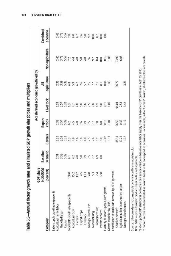
124 XINSHEN DIAO ET AL.
Tabl
e 5.5—
Annu
al fa
ctor
gro
wth
rate
s and
sim
ulat
ed G
DP g
rowt
h ela
stici
ties a
nd m
ultip
liers
GD
P sh
are
in
2005
/06
Base
line
Ex
port
Al
l
Com
bine
dCa
tego
ry
(per
cent
) sc
enar
io
Cere
als
crop
s Li
vest
ock
agric
ultu
re
Nona
gricu
lture
sc
enar
ioLa
bor s
upply
grow
th ra
te (p
erce
nt)
Ag
ricult
ural
family
labo
r
2.31
2.30
2.33
2.33
2.35
2.40
2.45
Un
skille
d lab
or
3.5
3 3.5
3 3.5
4 3.5
7 3.5
9 3.7
2 3.7
8
Capit
al
5.32
5.32
5.32
5.32
5.32
5.57
5.57
Total
GDP
grow
th ra
te (p
erce
nt)
100.0
6.1
6.3
6.2
6.3
6.8
7.2
7.8
Ag
ricult
ural
GDP
45.2
4.2
4.8
4.5
4.7
5.9
4.4
6.0
Ce
reals
13
.2 4.8
6.6
4.8
4.8
6.7
4.8
6.7
Expo
rt cro
ps
4.5
5.0
5.0
7.6
5.0
7.6
5.0
7.6
Liv
estoc
k 13
.3 3.9
4.0
3.9
5.6
5.7
4.0
5.8
No
nagr
icultu
ral G
DP
54.8
7.5
7.5
7.5
7.5
7.5
7.6
9.2
Manu
factur
ing
5.3
7.7
7.6
7.7
7.8
7.7
9.7
10.0
Agro
proc
essin
g 2.4
6.9
6.9
7.0
6.9
7.1
8.4
8.7
Pr
ivate
servi
ces
32.8
8.0
8.0
8.0
8.0
8.1
10.0
10.0
Elas
ticity
of la
bor s
upply
–GDP
a grow
th
–0
.02
0.15
0.11
0.06
0.10
0.09
Grow
th mu
ltiplie
r by 2
015
1.13
1.04
1.06
1.03
1.06
Contr
ibutio
n to t
otal G
DP in
creas
e by 2
015 (
perce
nt)
Sh
ocke
d sec
torsb
88.34
96
.50
94.04
96
.77
93.92
Agric
ultur
e rath
er th
an sh
ocke
d sec
tor
10.29
0.3
3 2.5
3
6.08
No
nagr
icultu
ral s
ector
s
1.3
7 3.1
7 3.4
2 3.2
3
Sour
ce: E
thiop
ian dy
nami
c com
putab
le ge
nera
l equ
ilibriu
m mo
del re
sults
.No
te: G
DP =
gros
s dom
estic
prod
uct. B
lank c
ells =
not a
pplic
able.
a Labo
r sup
ply–G
DP el
astic
ity is
defin
ed as
perce
ntage
chan
ge in
base
line t
otal la
bor s
upply
over
the b
aseli
ne G
DP gr
owth
rate,
both
for 20
15.
b Shoc
ked s
ector
s are
thos
e lab
eled a
s colu
mn he
ads i
n the
corre
spon
ding s
cena
rios.
For e
xamp
le, in
the “
Cere
als” c
olumn
, sho
cked
secto
rs ar
e cer
eals.
Acce
lerat
ed ec
onom
ic gr
owth
led
by
ETHIOPIA 125
whole, explains 10.3 percent of total GDP increase of 1.14 in that year (see the second-to-last row of Table 5.5). Insignifi cant growth-multiplier effects on non-agricultural sectors are due to diffi culty in labor mobility between the agricultural and nonagricultural sectors. To create more employment opportunities in non-agricultural sectors at a given wage rate requires improving productivity in these nonagricultural sectors, which was not considered in this scenario.
We turn next to the second scenario, in which export crops are the driving force behind accelerated economic growth. The fi rst fi nding is that the small size of this subsector in the economy (4.5 percent of total GDP in the base year) implies that even high growth rates in export crop value-added have only modest impacts on national GDP. The growth rate of agricultural GDP rises from 4.2 to 4.5 percent per year, and that for total GDP increases from 6.1 to 6.2 percent. These modest effects on the overall economy indicate that, although there is considerable potential to expand some export-oriented crops, its expected impact on the overall economy would be rather limited.
The second major fi nding from this scenario is that the growth multipliers for export crops are smaller than for cereals. An additional 0.04 units of GDP are cre-ated by a one unit increase in export-crop production. Moreover, the impact chan-nels are quite different. Unlike in cereal-led growth, the nonagricultural sector is positively affected by export crop–led growth, but the effect on other agricultural sectors is insignifi cant. Results indicate that 96.5 percent of increased GDP is a direct result of export-crop growth. Of the remaining impact channels, only 0.33 percent is attributable to nonexport agriculture, whereas 3.17 percent is due to nonagriculture.
The third fi nding is that export crop–led growth creates more employment opportunities, as growth rates in both family farm and unskilled labor increase from baseline levels. The reason is that export crops are produced for foreign markets, and demand in such markets is not constrained by domestic income. Without consider-ing other constraints, such as increased trade barriers from importing countries and physical and institutional diffi culties in accessing markets, productivity growth in export crops leads to increased demand for family and unskilled labor. Measured as a labor-supply–GDP elasticity, a 1 percent increase in GDP led by growth in export crops is associated with a 0.15 percent increase in total labor supply (in Table 5.5 in the fourth column in the row for “Elasticity of labor supply–GDP growth”). This is the highest elasticity in all of the scenarios we consider.
A comparison of the results from the fi rst two scenarios indicates that the con-tribution of an agricultural subsector’s growth to overall economic growth is mainly determined by the size of the subsector. Small subsectors may have high growth poten-tials but can only generate modest increases in overall economic growth. Furthermore, although the economywide multiplier effect of a subsector is important, it should
126 XINSHEN DIAO ET AL.
not be the only indicator used to explain growth linkages between agriculture and nonagriculture, as well as within agriculture. Given that the Ethiopian government has accorded a high priority to generating employment, promoting growth in some sectors can create more employment opportunities, even though they may not generate as much economywide growth. Those subsectors that face fewer demand constraints from domestic markets and that use unskilled labor more intensively will have greater potential to create jobs at the given level of growth.
Comparing Agriculture-Led and Nonagriculture-Led GrowthThe fourth and fi fth scenarios compare agricultural and nonagricultural growth. In reality it is impossible to have either the agricultural or nonagricultural sectors grow independently of each other. However, these two scenarios are designed to assess possible differential effects on the overall economic growth and poverty reduction. As shown in the fi rst two rows of Table 5.5, growth in the aggregate agricultural and nonagricultural sectors creates more employment opportunities both for family farm labor and unskilled labor, whereas nonagricultural growth leads to a greater increase in labor demand and therefore more employment opportunities than does growth in the agricultural sector alone. Measured by the labor-supply–GDP elastic-ity, a 1 percent increase in total GDP led by nonagricultural growth is associated with a 0.10 percent increase in labor supply, and the elasticity is 0.06 when agricul-tural growth is the leading force. Moreover, the growth multiplier in the case of nonagriculture-led growth is higher than that of agriculture-led growth (1.06 versus 1.03). Stronger growth-multiplier effects from nonagriculture-led growth are related to additional capital accumulation. Nonagriculture is more capital intensive than agriculture. Increases in nonagricultural productivity leads to faster investment growth, which generates additional demand for capital goods production. Faster capital accumulation creates more demand for labor that can be employed by both agricultural and nonagricultural sectors. This demand leads to higher growth-multiplier effects in this scenario. Decomposition of the multiplier effect shows that, in the agricultural growth scenario, only 3.24 percent of increased GDP (1.03 units) occurs in the nonagricultural sector, whereas in the nonagricultural growth scenario, 6.08 percent of the increase in GDP (1.06 units) comes from increased agricultural GDP.
Demand-side linkages are examined in Table 5.6. The fi rst panel in the table presents annual consumption growth rates in the various scenarios. The commodity groups shown in the table are aggregations from the 62 groups used in the DCGE model, with base year prices for each individual commodity used as weights. As shown in the table, the growth rate in real consumption is lower than the total GDP growth rate. This is because the change in relative prices and different income elas-ticities across commodities cause demand growth to vary across commodities.
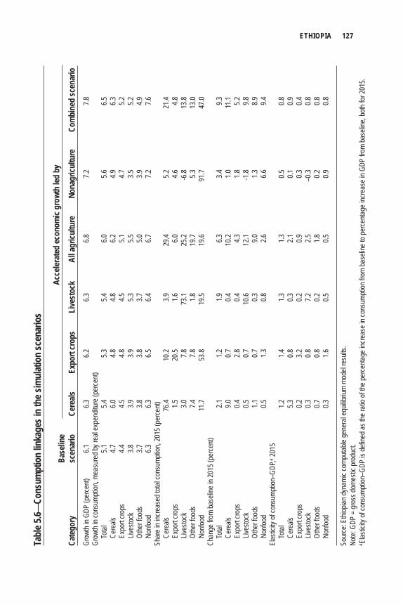
ETHIOPIA 127Ta
ble 5
.6—Co
nsum
ptio
n lin
kage
s in
the s
imul
atio
n sc
enar
ios
Ba
selin
e
Cate
gory
sc
enar
io
Cere
als
Expo
rt cr
ops
Live
stoc
k Al
l agr
icultu
re
Nona
gricu
lture
Co
mbi
ned
scen
ario
Grow
th in
GDP
(per
cent)
6.1
6.3
6.2
6.3
6.8
7.2
7.8
Grow
th in
cons
umpti
on, m
easu
red b
y rea
l exp
endit
ure (
perce
nt)
Total
5.1
5.4
5.3
5.4
6.0
5.6
6.5
Ce
reals
4.7
6.0
4.8
4.8
6.2
4.9
6.3
Ex
port
crops
4.4
4.5
4.8
4.5
5.1
4.7
5.2
Liv
estoc
k 3.8
3.9
3.9
5.3
5.5
3.5
5.2
Ot
her f
oods
3.7
3.8
3.8
3.7
5.0
3.9
4.9
No
nfood
6.3
6.3
6.5
6.4
6.7
7.2
7.6
Shar
e in i
ncre
ased
total
cons
umpti
on, 2
015 (
perce
nt)
Cere
als
76
.4 10
.2 3.9
29
.4 5.2
21
.4
Expo
rt cro
ps
1.5
20
.5 1.6
6.0
4.6
4.8
Liv
estoc
k
3.0
7.8
73.1
25.2
-6.8
13.8
Ot
her f
oods
7.4
7.8
1.8
19.7
5.3
13.0
No
nfood
11.7
53.8
19.5
19.6
91.7
47.0
Chan
ge fr
om ba
selin
e in 2
015 (
perce
nt)
Total
2.1
1.2
1.9
6.3
3.4
9.3
Cere
als
9.0
0.7
0.4
10
.2 1.0
11
.1
Expo
rt cro
ps
0.4
2.8
0.4
4.3
1.8
5.2
Liv
estoc
k
0.5
0.7
10.6
12.1
-1.8
9.8
Othe
r foo
ds
1.1
0.7
0.3
9.0
1.3
8.9
No
nfood
0.5
1.3
0.8
2.6
6.6
9.4El
astic
ity of
cons
umpti
on–G
DP,a 20
15
Total
1.2
1.4
1.3
1.3
0.5
0.8
Cere
als
5.3
0.8
0.3
2.1
0.1
0.9
Ex
port
crops
0.2
3.2
0.2
0.9
0.3
0.4
Lives
tock
0.3
0.8
7.2
2.5
–0
.3 0.8
Ot
her f
oods
0.7
0.8
0.2
1.8
0.2
0.8
Nonfo
od
0.3
1.6
0.5
0.5
0.9
0.8
Sour
ce: E
thiop
ian dy
nami
c com
putab
le ge
nera
l equ
ilibriu
m mo
del re
sults
.No
te: G
DP =
gros
s dom
estic
prod
uct.
a Elas
ticity
of co
nsum
ption
–GDP
is de
fined
as th
e rati
o of th
e per
centa
ge in
creas
e in c
onsu
mptio
n fro
m ba
selin
e to p
erce
ntage
incre
ase i
n GDP
from
base
line,
both
for 20
15.
Ac
celer
ated
econ
omic
grow
th le
d by
128 XINSHEN DIAO ET AL.
Comparing consumption growth rates for the fi rst two scenarios reveals that consumption for a group of commodities grows more rapidly when the group is targeted in the scenario. For example, the growth rate of cereal consumption in-creases from 4.7 to 6.0 percent in the cereal-led growth scenario. However, in the same scenario, livestock consumption growth only increases slightly. In contrast, when growth is led by additional livestock productivity, livestock consumption grows more rapidly, while cereal consumption growth rate rises only slightly. This differential demand effect by commodity groups is due to relative prices. Accelerating growth in a particular group of commodities causes its prices to fall relative to other commodity groups. This growth generates additional incomes for the farmers engaged in these subsectors, but increased consumption stemming from direct income effects is not limited to those products for which supply increases. On the contrary, lower prices induce more across-the-board consumption by both rural and urban households. When accelerated growth occurs across the whole economy, rela-tive price movements become smaller, and growth in consumption is dominated by income effects. Thus, growth differences across commodity groups also decrease.
The second panel in Table 5.6 reports the contribution of each commodity group to the increase in total consumption. It shows that when accelerated growth is led by cereals, then 76.4 percent of increased total consumption is from cereal consumption itself. When growth is led by the livestock subsectors, then live-stock consumption explains 73.1 percent of total consumption increases. More importantly, when growth is led by export crops then 53.8 percent of consumption increases are from nonagricultural goods. Such differential consumption outcomes will have effects on poverty reduction. For a low-income country like Ethiopia, most of the poor population lives in rural areas, where food consumption, particularly staple foods, is the most important component of household total expenditure baskets (including expenditure in kind). When economic growth increases income among rural low-income households, then staple consumption grows more rapidly than consumption of other commodities. This differential occurs because rural poor households have higher income elasticities for food demand than do urban and nonpoor rural households. In the poverty–growth linkage analysis below, we show that agriculture-led growth is more pro-poor than growth led by the nonagricultural sector. One important reason for this is due to the different effects on consumption growth across different scenarios shown in Table 5.6.
The fi nal panel of Table 5.6 shows the ratio of changes in consumption to changes in total GDP, which can be used to compare the marginal effect of growth led by different subsectors on consumption of the various commodity groups. The table shows that the consumption–growth elasticity is higher under agriculture-led growth than under nonagriculture-led growth. This trend is particularly evident for
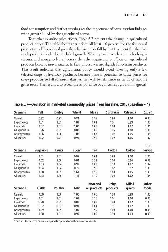
ETHIOPIA 129
food consumption and further emphasizes the importance of consumption linkages when growth is led by the agricultural sector.
To further examine price effects, Table 5.7 presents the change in agricultural product prices. The table shows that prices fall by 8–16 percent for the fi ve cereal products under cereal-led growth, whereas prices fall by 9–11 percent for the live-stock products under livestock-led growth. When growth accelerates in both agri-cultural and nonagricultural sectors, then the negative price effects on agricultural products become much smaller. In fact, prices even rise slightly for certain products. This result indicates that agricultural policy should avoid favoring only a few selected crops or livestock products, because there is potential to cause prices for these products to fall so much that farmers will benefi t little in terms of income generation. The results also reveal the importance of concurrent growth in agricul-
Table 5.7—Deviation in marketed commodity prices from baseline, 2015 (baseline = 1)
Scenario Teff Barley Wheat Maize Sorghum Oilseeds EnsetCereals 0.92 0.87 0.84 0.85 0.90 1.00 0.97Export crops 1.01 1.01 1.01 1.01 1.01 0.99 1.00Livestock 1.02 1.02 1.02 1.03 1.03 1.02 1.01All agriculture 0.96 0.91 0.88 0.89 0.95 1.00 1.00Nonagriculture 1.06 1.06 1.06 1.07 1.07 1.05 1.05All sectors 1.02 0.97 0.93 0.96 1.02 1.06 1.07
CutScenario Vegetable Fruits Sugar Tea Cotton Coffee flowersCereals 1.01 1.01 0.98 1.01 0.99 1.00 1.00Export crops 1.02 1.00 0.84 0.91 0.68 0.96 0.99Livestock 1.03 1.04 0.99 1.03 0.98 1.02 1.02All agriculture 1.04 1.04 0.79 0.95 0.67 0.97 1.01Nonagriculture 1.08 1.21 1.61 1.15 1.60 1.05 1.03All sectors 1.13 1.26 1.44 1.10 1.04 1.02 1.04 Meat and Dairy Milled OtherScenario Cattle Poultry Milk oil products products grains foods Cereals 1.00 1.00 1.00 1.00 1.00 0.99 1.00Export crops 1.01 1.01 1.01 0.98 1.01 1.00 0.98Livestock 0.90 0.91 0.89 1.03 0.90 1.02 1.03All agriculture 0.92 0.92 0.91 1.01 0.91 1.02 1.01Nonagriculture 1.09 1.09 1.09 0.99 1.09 1.00 0.98All sectors 1.00 1.01 0.99 1.00 0.99 1.03 0.99
Source: Ethiopian dynamic computable general equilibrium model results.
130 XINSHEN DIAO ET AL.
tural and nonagricultural sectors for stabilizing agricultural prices—an important linkage effect that can only be observed in a general equilibrium analysis.
Decomposing Agricultural Growth’s Impact on PovertyAccelerating economic growth is often the primary focus of policy interventions in low-income countries like Ethiopia, because only rapid growth can enable the country to catch up with the rest of the world. The previous subsection showed the importance of agriculture in generating overall growth and demonstrated that this importance is not only because of the size of agriculture. Rather, the importance of agriculture is also due to its strong linkages to the rest of the economy, particular consumption linkages, which allow growth to directly benefi t a majority of the popu-lation and increase consumption levels. In this subsection, we focus on the impact of growth on poverty reduction, one of the most important goals for all developing countries.
Although growth is generally good for the poor, opportunities for them to participate in growth varies, depending on the type of growth. The growth–poverty linkage analysis addresses this issue and measures what kind of growth creates more job opportunities for the poor. We use similar scenarios to those from the growth linkage analysis to evaluate the linkages between growth led by different subsectors and poverty reduction. Although income distribution infl uences the effectiveness of growth on poverty reduction, we are unable to analyze its effect in the current model structure. That is to say, we generally assume that the income distribution, particularly the distribution in each representative household group, does not change over time for different types of growth. Although this caveat of the model may lead to an overestimation of growth’s contribution to poverty reduction, it will not be a problem when the focus of the analysis is to compare growth–poverty link-ages across different scenarios designed in the model. We explain this argument below.
To compare the effectiveness of growth led by different subsectors on poverty reduction, it is important to make sure scenarios are comparable. Because of the different sizes of the subsectors, the same growth rate at the subsector level can have very different impacts on national economic growth and poverty reduction. It is unlikely that a small subsector will cause large reductions in poverty, even if this small sector grows rapidly. To address this comparability issue, we focus on the link-age between overall economic growth and poverty reduction. The poverty–growth elasticity is calculated using the same formula as before (the percentage change in the national poverty rate caused by 1 percent growth in per capita GDP).
According to 2004/05 HICES (Ethiopia, CSA 2005), the country’s reported national poverty rate was 38.7 percent in 2005. This poverty rate is consistent with the standard US$1.25 per capita per day international measure of poverty. As
ETHIOPIA 131
expected, the rural poverty rate is similar to the national poverty rate, because more than 80 percent of the population lives in rural areas. The rural poverty rate is 39.3 percent, and the urban rate is slightly lower (35.1 percent).
It is widely anticipated that Ethiopia is unlikely to meet the fi rst Millennium Development Goal of halving poverty by 2015, which requires the poverty rate fall to 23 percent by 2015. We fi rst use the Ethiopian model to simulate baseline poverty reduction, consistent with the baseline growth simulation. According to our results, the national poverty rate will fall to 28.6 percent by 2015 (Table 5.8). Obviously, Ethiopia needs to not only accelerate the level of growth but also fi nd ways to en-hance the benefi ts of growth for its poor. In other words, it is important to identify the composition of growth that is most effective at reducing poverty. In this regard, it is necessary to consider the relative importance of agriculture and industry in helping the country signifi cantly reduce poverty.
Using the same six scenarios discussed above, the growth–poverty linkages are used to compare the effectiveness of additional growth in reducing poverty under different growth assumptions. The poverty–growth elasticity is calculated for each scenario based on growth in total GDP rather than on the sector’s GDP. Table 5.8 shows the poverty rate by 2015 in each scenario. For example, the national rate falls to 28.6 percent in 2015 in the model’s baseline, and the rural and urban poverty rates fall to 29.6 and 23.5 percent, respectively. With one exception, all poverty rates fall more in the six accelerated growth scenarios. The national poverty rate falls to 23.9 percent in 2015 in the sixth growth scenario (all sectors combined)—a poverty rate that nearly achieves the country’s fi rst Millennium Development Goal.
The second panel of Table 5.8 reports the additional number of people lifted above the poverty line by 2015 in each growth scenario. About 25 million people were living below the poverty line in 2005. The baseline scenario lowers this number to 24 million. Considering that the population will grow by 19.5 to 20 million over the 10-year simulation period (with a 2.7 percent population growth rate), the decline in the absolute number of poor under the baseline seems to be an optimistic scenario. The model results also indicate that about 60 percent of the reduction in the number of poor occurs in rural areas (not shown in the table). The model there-fore reports more optimistic poverty reduction in urban areas, where the poverty rate falls to 23.5 percent by 2015—an 11.6 percentage point reduction from its level in 2005. The fi nal row of the table reports poverty–growth elasticity, which was 1.13 in the baseline. We have mentioned in previous subsections that this elasticity is higher than that calculated using historical data, but it is comparable to those of other countries derived using similar methods.
We now assess how different sources of growth affect poverty reduction rates dif-ferentially. We start with the agriculture-led and nonagriculture-led scenarios. As dis-cussed above, the annual GDP growth rate is 6.8 and 7.2 percent in the agriculture-led
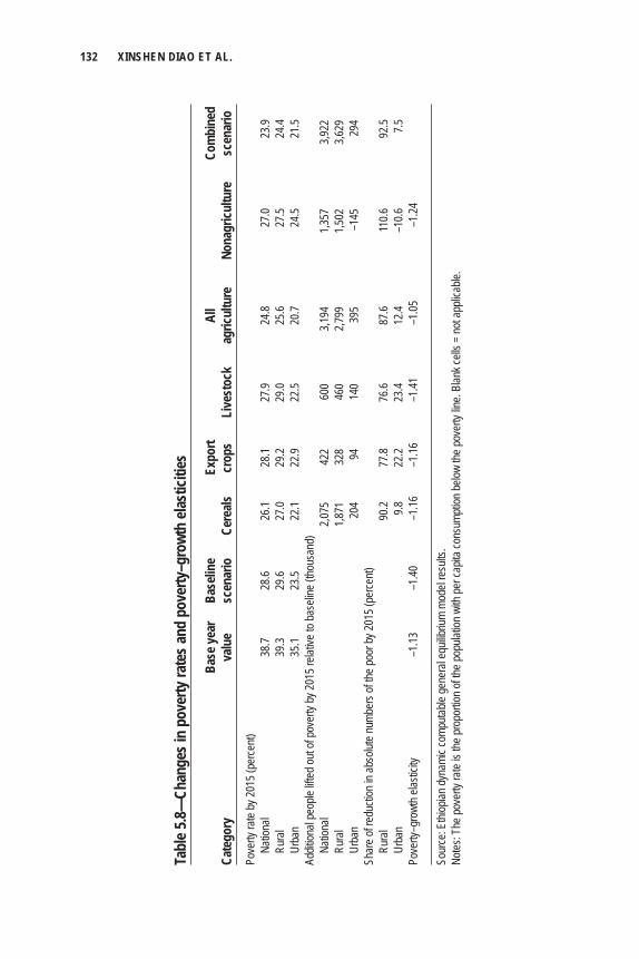
132 XINSHEN DIAO ET AL.
Tabl
e 5.8—
Chan
ges i
n po
verty
rate
s and
pov
erty
–gro
wth
elast
icitie
s
Ba
se ye
ar
Base
line
Ex
port
Al
l
Com
bine
dCa
tego
ry
valu
e sc
enar
io
Cere
als
crop
s Li
vest
ock
agric
ultu
re
Nona
gricu
lture
sc
enar
ioPo
verty
rate
by 20
15 (p
erce
nt)
Natio
nal
38.7
28.6
26.1
28.1
27.9
24.8
27.0
23.9
Ru
ral
39.3
29.6
27.0
29.2
29.0
25.6
27.5
24.4
Ur
ban
35.1
23.5
22.1
22.9
22.5
20.7
24.5
21.5
Addit
ional
peop
le lift
ed ou
t of p
over
ty by
2015
relat
ive to
base
line (
thous
and)
Na
tiona
l
2,0
75
422
600
3,194
1,3
57
3,922
Ru
ral
1,871
32
8 46
0 2,7
99
1,502
3,6
29
Urba
n
20
4 94
14
0 39
5 –1
45
294
Shar
e of r
educ
tion i
n abs
olute
numb
ers o
f the p
oor b
y 201
5 (pe
rcent)
Ru
ral
90.2
77.8
76.6
87.6
110.6
92
.5
Urba
n
9.8
22
.2 23
.4 12
.4 –1
0.6
7.5Po
verty
–gro
wth e
lastic
ity
–1.13
–1
.40
–1.16
–1
.16
–1.41
–1
.05
–1.24
Sour
ce: E
thiop
ian dy
nami
c com
putab
le ge
nera
l equ
ilibriu
m mo
del re
sults
.No
tes: T
he po
verty
rate
is the
prop
ortio
n of th
e pop
ulatio
n with
per c
apita
cons
umpti
on be
low th
e pov
erty
line.
Blan
k cell
s = no
t app
licab
le.
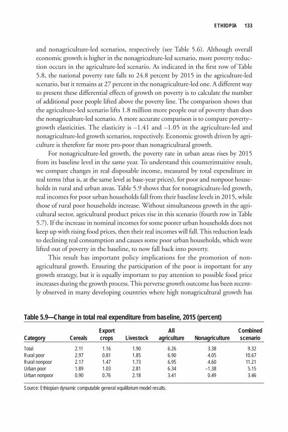
ETHIOPIA 133
and nonagriculture-led scenarios, respectively (see Table 5.6). Although overall economic growth is higher in the nonagriculture-led scenario, more poverty reduc-tion occurs in the agriculture-led scenario. As indicated in the fi rst row of Table 5.8, the national poverty rate falls to 24.8 percent by 2015 in the agriculture-led scenario, but it remains at 27 percent in the nonagriculture-led one. A different way to present these differential effects of growth on poverty is to calculate the number of additional poor people lifted above the poverty line. The comparison shows that the agriculture-led scenario lifts 1.8 million more people out of poverty than does the nonagriculture-led scenario. A more accurate comparison is to compare poverty–growth elasticities. The elasticity is –1.41 and –1.05 in the agriculture-led and nonagriculture-led growth scenarios, respectively. Economic growth driven by agri-culture is therefore far more pro-poor than nonagricultural growth.
For nonagriculture-led growth, the poverty rate in urban areas rises by 2015 from its baseline level in the same year. To understand this counterintuitive result, we compare changes in real disposable income, measured by total expenditure in real terms (that is, at the same level as base-year prices), for poor and nonpoor house-holds in rural and urban areas. Table 5.9 shows that for nonagriculture-led growth, real incomes for poor urban households fall from their baseline levels in 2015, while those of rural poor households increase. Without simultaneous growth in the agri-cultural sector, agricultural product prices rise in this scenario (fourth row in Table 5.7). If the increase in nominal incomes for some poorer urban households does not keep up with rising food prices, then their real incomes will fall. This reduction leads to declining real consumption and causes some poor urban households, which were lifted out of poverty in the baseline, to now fall back into poverty.
This result has important policy implications for the promotion of non-agricultural growth. Ensuring the participation of the poor is important for any growth strategy, but it is equally important to pay attention to possible food price increases during the growth process. This perverse growth outcome has been recent-ly observed in many developing countries where high nonagricultural growth has
Table 5.9—Change in total real expenditure from baseline, 2015 (percent)
Export All CombinedCategory Cereals crops Livestock agriculture Nonagriculture scenarioTotal 2.11 1.16 1.90 6.26 3.38 9.32Rural poor 2.97 0.81 1.85 6.90 4.05 10.67Rural nonpoor 2.17 1.47 1.73 6.95 4.60 11.21Urban poor 1.89 1.03 2.81 6.34 –1.38 5.15Urban nonpoor 0.90 0.76 2.18 3.41 0.49 3.46
Source: Ethiopian dynamic computable general equilibrium model results.
134 XINSHEN DIAO ET AL.
been accompanied by food price infl ation. Ethiopia appears to have shown this same outcome during its recent growth period, which may partly explain why rapid growth has not signifi cantly reduced poverty in urban areas.
ConclusionsEthiopia has embarked on an agriculture-led growth strategy to meet the challenges of accelerating national growth and poverty reduction. Three sets of questions around the importance of the agricultural sector were highlighted as being relevant to the implementation of this strategy. Which sectors have large prospective link-ages? What are the growth and poverty-reduction potential of these sectors? What policy interventions are needed to unlock their growth potential? We have applied the DCGE model described in Chapter 2 to address these three policy questions for Ethiopia. Several key messages can be drawn from our analysis.
First, the importance of agriculture relates to its size in the economy. Although the agricultural sector is unlikely to grow faster than many nonagricultural sub-sectors, due in part to its greater dependency on nature, its size is much larger than the nonagricultural sector in Ethiopia. The country’s economic history shows that GDP growth is strongly correlated with agricultural growth. The DCGE model showed that agricultural growth, even when it is slower than nonagricultural growth, directly contributes more to overall economic growth. Moreover, certain large staple subsectors drive the agricultural sector as a whole. In contrast, some nontraditional export crop sectors may be able to grow very rapidly, but this growth will be from a small base and so is unlikely to translate into signifi cant sectorwide growth. For this reason, overall agricultural growth must primarily come from growth in the staple subsectors.
Second, the importance of cereal production in overall economic growth is due not only to its size but also to its strong multiplier effects. The model shows that cereal-led growth has the largest multiplier effect and is a driver of growth in other agricultural subsectors.
Third, there exists a certain limitation to cereal-led growth for job creation. In fact, productivity-led growth in the cereal sector will release labor from agriculture, which requires that other sectors of the economy absorb more labor. Because Ethiopia is a labor-abundant economy with rapid population growth, it is necessary to pay attention to limited job creation potential when promoting cereal production. Export crops, in contrast, may have smaller growth multipliers, but they create more employ-ment opportunities, because they face less stringent demand constraints and relatively stronger linkages with market activities (including trade and transport).
Fourth, the growth multiplier effect is higher in the nonagricultural sector than it is in the agricultural sector as a whole. These enhanced multiplier effects are related to the current structure of Ethiopia’s nonagricultural sector and the growth assump-
ETHIOPIA 135
tions of the model. In the model’s simulation, additional nonagricultural growth mainly comes from manufacturing and private services. Agroprocessing is one of the most important components of manufacturing in Ethiopia, and private services are primarily for meeting domestic demand. Thus, accelerated growth in these nonagricultural subsectors is expected to create demand for agricultural goods, both through production and consumption linkages. Moreover, such nonagricultural growth is good for job creation, because it increases labor demand in both agricul-tural and nonagricultural sectors. However, more private investments and higher growth rates in capital accumulation are the preconditions for greater multiplier effects and job creation in the nonagricultural sector. Incentives for the private sector to invest can be discouraged in a business environment that has institutional barri-ers. These will constrain nonagricultural growth led by the private sector and hence limit job creation. The model did not consider these constraints, which should ideally be taken into consideration for Ethiopia.
Fifth, real prices for staple crops and livestock products are expected to fall when growth in these agricultural subsectors is faster than growth in other sectors of the economy. Urban consumers as well as farmers who are net buyers of foodcrops and livestock products will benefi t from such declines in prices. Conversely, farmers who are net sellers of these products will be hurt by lower incomes. Thus, it is essential to pay close attention to any potential negative effects on famer income induced by falling prices when agricultural policies favor only a few crops or livestock products. The simulation results also reveal the importance of concurrent growth of agricul-tural and nonagricultural sectors for stabilizing agricultural prices—an important linkage effect that can only be observed though general equilibrium analysis.
Sixth, the impact of growth on poverty is larger when economywide growth is driven by agriculture rather than by nonagriculture. Agriculture-led growth can lift 1.4 times more people out of poverty than the same amount of nonagriculture-led growth.
Finally, nonagriculture-led growth can become less pro-poor even in urban areas when such growth causes domestic food prices to rise. This result has impor-tant policy implications when promoting nonagricultural growth. Although the participation of the poor in the growth process is important for promoting any form of growth, it is equally important to pay attention to possible food price increases from neglecting agriculture. This kind of growth outcome has recently been observed in many developing countries where high nonagricultural growth has been accom-panied by food price infl ation. It may also explain the slowdown in poverty reduc-tion in Ethiopia’s urban areas.
This chapter quantitatively measured growth linkages and growth–poverty relationships by assuming that economywide growth is driven by accelerated growth in different sectors or subsectors of agriculture. Nevertheless, it is not the intention of this analysis to prioritize particular sectors for Ethiopia’s growth strategy. Rather,
136 XINSHEN DIAO ET AL.
our analysis reveals differential roles for economic sectors in generating both growth and poverty reduction and hence displays their interdependence during the develop-ment process.
Government policies and public investments are important conditions for productivity-led growth in the economy. However, they are not assessed in this chapter. Moreover, to stimulate the same level of economic growth across different subsectors may require different levels of public investment. We did not use the Ethiopian DCGE model for cost–benefi t assessment. Moreover, growth at the sub-sector level is not necessarily the result of public investment. Investment by the private sector is often the dominant force in generating growth in the nonagricultural sector and in export-oriented high-value agriculture. In this case, the existence of a dynam-ic private sector requires policy supports and appropriate institutional environ-ments. These factors are often more important for capital accumulation than public sector direct intervention.
In the agricultural sector, both better incentives and improved production conditions are needed to provide farmers with more opportunities to diversify and consequently to transition many crops currently grown for subsistence into market-able commodities and cash income opportunities. Policies and public investments that will help improve agricultural production and market conditions and encour-age farmers to improve land and labor productivity are also necessary. The main elements of the Ethiopian government’s approach to improving market connectivity have focused on the crucial areas of liberalizing markets and improving roads, espe-cially major highways. Liberalization has improved the functioning of grain markets after the interventionist policies of the Derg, particularly in regions that produce surplus grain (World Bank 2006). The government has recognized that a dramati-cally improved road network is a prerequisite for enhanced growth in agriculture and for fostering urban–rural linkages. However, transport costs for farmers and traders remain high, despite a signifi cant effort over the past decade on road con-struction. This is in part because most farmers lack feeder roads to the main net-works, and roads are long-term and costly investments that do not improve yields or generate positive returns quickly. However, it is broadly accepted that growth in the agricultural sector is constrained by the service sector, including trade, transport, and fi nancial and business services. Improvements in these market-related services will strengthen intersectoral linkages and increase growth-multiplier effects. Moreover, reducing marketing costs benefi ts smallholders by increasing the net prices they receive for their goods, thereby raising incomes. Improving market con-ditions also creates a more effi cient trading sector, which itself can increase non-agricultural incomes without necessarily raising costs.
Looking beyond road investments, supportive policy measures are also needed to develop functioning markets. Institution building and attention to risk, informa-tion, and distortions related to food aid are also critical (Gabre-Madhin 2001). The
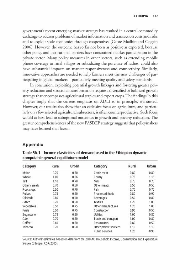
ETHIOPIA 137
government’s recent emerging-market strategy has resulted in a central commodity exchange to address problems of market information and transaction costs and risks and to exploit scale economies through cooperatives (Gabre-Madhin and Goggin 2006). However, the outcome has so far not been as positive as expected, because other policy and institutional barriers have constrained market participation in the private sector. Many policy measures in other sectors, such as extending mobile phone coverage to rural villages or subsidizing the purchase of radios, could also have substantial impacts on market responsiveness and connectivity. Similarly, innovative approaches are needed to help farmers meet the new challenges of par-ticipating in global markets—particularly meeting quality and safety standards.
In conclusion, exploiting potential growth linkages and fostering greater pov-erty reduction and structural transformation require a diversifi ed or balanced growth strategy that encompasses agricultural staples and export crops. The fi ndings in this chapter imply that the current emphasis on ADLI is, in principle, warranted. However, our results also show that an exclusive focus on agriculture, and particu-larly on a few selected agricultural subsectors, is often counterproductive. Such focus would at best lead to suboptimal outcomes in growth and poverty reduction. The greater comprehensiveness of the new PASDEP strategy suggests that policymakers may have learned that lesson.
Appendix
Table 5A.1—Income elasticities of demand used in the Ethiopian dynamic computable general equilibrium model
Category Rural Urban Category Rural UrbanMaize 0.70 0.50 Cattle meat 0.80 0.80Wheat 1.00 0.66 Poultry 0.75 1.15Teff 1.10 0.70 Milk 0.75 0.75Other cereals 0.70 0.50 Other meats 0.50 0.50Root crops 0.50 0.70 Fish 0.70 0.70Pulses 0.75 0.60 Processed foods 0.80 0.90Oilseeds 0.80 0.50 Beverages 0.50 0.80Enset 0.70 0.50 Textiles 1.20 1.00Vegetables 0.50 0.75 Other manufactures 1.20 1.00Fruits 0.50 0.75 Construction 0.90 0.50Sugarcane 0.75 0.60 Utilities 1.00 0.80Chat 0.70 0.50 Trade and transport 1.00 0.80Coffee 0.60 0.60 Restaurants 0.80 0.50Tobacco 0.70 0.50 Other private services 1.10 1.10 Public services 1.20 0.90
Source: Authors’ estimates based on data from the 2004/05 Household Income, Consumption and Expenditure Survey (Ethiopia, CSA 2005).
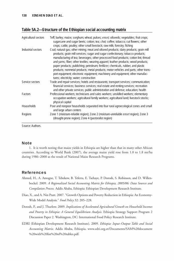
138 XINSHEN DIAO ET AL.
Table 5A.2—Structure of the Ethiopian social accounting matrix
Agricultural sectors Teff; barley; maize; sorghum; wheat; pulses; enset; oilseeds; vegetables; fruit crops; sugarcane and sugar beets; cotton; tea; chat; coffee; tobacco; cut flowers; other
crops; cattle; poultry; other small livestock; raw milk; forestry; fishingIndustrial sectors Coal; natural gas; other mining; meat and oilseed products; dairy products; grain mill products; grain mill services; sugar and sugar confectionary; tobacco products;
manufacturing of tea; beverages; other processed food products; cotton lint; thread and yarns; fiber; other textiles; wearing apparel; leather products; wood products; paper products; publishing; petroleum; fertilizer; chemicals, rubber, and plastic products; nonmetal products; metal products; motor vehicles and parts; other trans-port equipment; electronic equipment; machinery and equipment; other manufac-tures; electricity; water; construction
Service sectors Trade and repair services; hotels and restaurants; transport services; communication; financial services; business services; real estate and renting services; recreation
and other private services; public administration and defense; education; healthFactors Professional workers; technicians and sales workers; unskilled workers; elementary occupation workers; agricultural family workers; agricultural land; livestock stocks;
physical capitalHouseholds Poor and nonpoor households separated into four rural agroecological zones and small and large urban centersRegions Zone 1 (moisture-reliable region); Zone 2 (moisture-unreliable enset region); Zone 3 (drought-prone region); Zone 4 (pastoralist region)
Source: Authors.
Note 1. It is worth noting that maize yields in Ethiopia are higher than that in many other African countries. According to World Bank (2007), the average maize yield rose from 1.0 to 1.8 mt/ha during 1986–2000 as the result of National Maize Research Programs.
References Ahmed, H., A. Amogne, T. Tebekew, B. Teferra, E. Tsehaye, P. Dorosh, S. Robinson, and D. Willen-
bockel. 2009. A Regionalized Social Accounting Matrix for Ethiopia, 2005/06: Data Sources and
Compilation Process. Addis Ababa, Ethiopia: Ethiopian Development Research Institute.
Diao, X., and A. Nin Pratt. 2007. “Growth Options and Poverty Reduction in Ethiopia: An Economy-
Wide Model Analysis.” Food Policy 32: 205–228.
Dorosh, P., and J. Thurlow. 2009. Implications of Accelerated Agricultural Growth on Household Incomes
and Poverty in Ethiopia: A General Equilibrium Analysis. Ethiopia Strategy Support Program 2
Discussion Paper 2. Washington, DC: International Food Policy Research Institute.
EDRI (Ethiopian Development Research Institute). 2009. Ethiopia: Input–Output Table and Social
Accounting Matrix. Addis Ababa, Ethiopia. www.edri.org.et/Documents/SAM%20document
%20with%20list%20of%20tables.pdf.
ETHIOPIA 139
Ethiopia, CSA (Central Statistical Agency). 2004. Report on Area and Production of Belg Season Crops
for Private Peasant Holdings. Statistical Bulletin 302. Addis Ababa, Ethiopia: Federal Democratic
Republic of Ethiopia.
———. 2005. Household Income, Consumption, and Expenditure Survey 2004/2005. Addis Ababa,
Ethiopia: Federal Democratic Republic of Ethiopia.
———. 2008a. Agricultural Sample Survey 2007/2008 (2000 E.C.): Volume I—Report on Area and
Production Crops (Private Peasant Holdings, Meher Season). Statistical Bulletin 417. Addis Ababa,
Ethiopia: Federal Democratic Republic of Ethiopia.
———. 2008b. Agricultural Sample Survey 2007/2008 (2000 E.C.): Volume III—Report on Farm
Management Practices (Private Peasant Holdings, Meher Season). Statistical Bulletin 417. Addis
Ababa, Ethiopia: Federal Democratic Republic of Ethiopia.
Ethiopia, CSA (Central Statistical Agency), EDRI (Ethiopian Development Research Institute), and
IFPRI (International Food Policy Research Institute). 2010. The Population and Housing Census
Atlas of Ethiopia 2007. Addis Ababa, Ethiopia; Washington, DC. www.csa.gov.et/pdf/atlas%20
cencus%202007.pdf.
Ethiopian Roads Transport Authority. 2006. “Ethiopian Road Network.” Dataset. Addis Ababa,
Ethiopia.
Gabre-Madhin, E. Z. 2001. Market Institutions, Transaction Costs, and Social Capital in the Ethiopian Grain
Market. Research Report 124. Washington, DC: International Food Policy Research Institute.
Gabre-Madhin, E. Z., and I. Goggin. 2006. “Does Ethiopia Need a Commodity Exchange? An
Integrated Approach to Market Development.” Paper presented at the Ethiopia Strategy Support
Program Conference, Addis Ababa, Ethiopia, June 6–8.
MOFED (Ministry of Finance and Economic Development ). 2002. Ethiopia: Sustainable Development
and Poverty Reduction Program. Addis Ababa, Ethiopia: Federal Democratic Republic of Ethiopia.
———. 2005. Ethiopia: Building on Progress: A Plan for Accelerated and Sustained Development to End
Poverty (PASDEP) (2005/06–2009/10). Addis Ababa, Ethiopia: Federal Democratic Republic of
Ethiopia.
Taffesse, A. S. 2007. “Product Flows and Growth Linkages in Ethiopia—A Note.” In Fostering New
Development Pathways: Harnessing Rural-Urban Linkages (RUL) to Reduce Poverty and Improve
Environment in the Highlands of Ethiopia: Proceedings of a Planning Workshop on Thematic Research
Area of the Global Mountain Program (GMP) Held in Addis Ababa, Ethiopia, August 29–30, 2006,
edited by Gete Zeleke, Peter Trutmann, Aster Denekew, 141–156. Lima, Peru; Addis Ababa,
Ethiopia: Global Mountain Program.
World Bank. 2006. Ethiopia: Policies for Pro-Poor Agricultural Growth. Washington, DC.
———. 2007. Ethiopia: Accelerating Equitable Growth—Country Economic Memorandum. Washington,
DC.
———. 2011. World Development Indicators. Washington, DC.

C h a p t e r 6
GhanaClemens Breisinger, Xinshen Diao, James Thurlow,
Samuel Benin, and Shashidhara Kolavalli
Ghana has experienced persistent growth with a record of positive per capita gross domestic product (GDP) growth over the past 26 years. As a result, the country is bound to become the first Sub-Saharan African country to
achieve the first Millennium Development Goal (MDG1) of halving poverty and hunger ahead of the target year 2015. Underlying this success are the country’s significant efforts to build institutions and state capacity. Ghana has become a stable democratic state, as demonstrated in a peaceful transition of power in two consecutive free and fair elections in 2000 and 2008. Governance indicators have been steadily improving over the past years, and in 2007 Ghana ranked ahead of regional averages of Asia, Latin America, and Africa in most important governance indicators, including government effectiveness, regulatory quality, and control of corruption (Kaufmann, Kraay, and Mastruzzi 2009). The country is ranked among the top 10 African countries in terms of freedom of the press and academic freedom (Freedom House 2008). Financial market development has made remark-able progress over the past years, including improvements in the banking sector, increasing trade volumes in the stock exchange, and the launch of government bonds. The domestic tax base has been broadened significantly over the past years, marking an important step toward reducing dependence on cocoa for government revenues. Decentralization has improved the allocation of public resources and the provision of services to address regional disparities (Bogetic et al. 2007). Perhaps most importantly, Ghanaians are determined to reach middle-income status and catch up with successful transformation countries in Asia, such as Korea, Malaysia, and Thailand, all of which started out at lower per capita income levels in the early 1960s than Ghana.
142 CLEMENS BREISINGER ET AL.
Although the share of agriculture in total GDP has declined and the service sector has replaced the agricultural sector to become the largest component of the economy in recent years, agriculture remains the most important sector for employ-ment. Agriculture continues to grow at a rate consistent with the overall economy, but its growth is not driven by productivity growth. Yields of most crops are still far below their potentials, and the level of modern technology adoption in agricultural production and processing is still extremely low. Agriculture remains highly depen-dent on rainfall: irrigation in Ghana is used on only 3 percent of total crop area, and less than 20 percent of irrigation potential is realized. In contrast, the potential for land expansion has been reaching its limits in some agroecological zones, urging a rapid shift toward productivity-led growth to transform traditional agriculture.
Against this background, the Government of Ghana has chosen to make the agricultural sector a key part of its development plan. To analyze the role of agricul-tural growth acceleration for Ghana’s future development, the recursive dynamic computable general equilibrium (DCGE) model described in Chapter 2 is used for the analysis of growth options and poverty reduction. The remainder of the chapter is structured as follows. We fi rst review the structure of Ghana’s agricultural sector, including its recent growth performance. We then describe the structure of the Ghanaian DCGE model and its underlying data sources. The model results are presented for the baseline and accelerated growth scenarios, and then for the invest-ment analysis. The latter is based on country-specifi c regression analysis. The fi nal section draws together our fi ndings from the Ghanaian case study and identifi es policy options for realizing the potential for agricultural growth and poverty reduction.
Agriculture in GhanaAgriculture in Ghana accounts for more than 30 percent of GDP and three-quarters of export earnings. It employs 60 percent of the labor force. With an average annual rate of 5.5 percent, Ghana’s recent agricultural growth has been more rapid than growth in its nonagricultural sectors (World Bank 2007). Moreover, in contrast to growth in the early period (Table 6.1), the main driving factor behind the recent rapid agricultural growth is the crop subsector (excluding cocoa), the largest sub-sector in agriculture, accounting for more than two-thirds of the agricultural econ-omy. Staple crops, including maize, sorghum, rice, cassava, yams, plantains, pulses, and oilseeds, dominate this subsector. Some high-value crops, such as vegetables and fruits, are also included, but they play a relatively modest role in overall agricultural growth because they make up a small share of the sector.
Cocoa is Ghana’s most important traditional export crop and has received special attention from the government in terms of fi nancial and policy supports. As
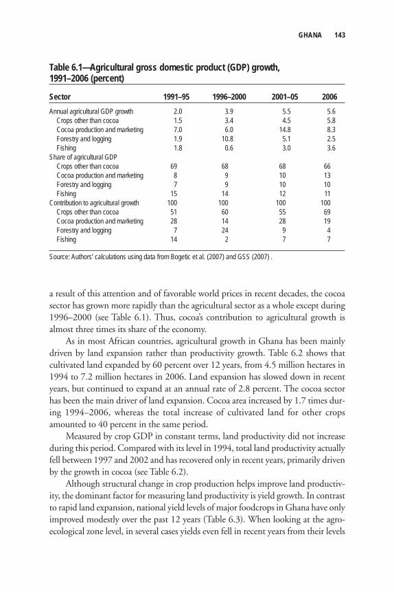
GHANA 143
a result of this attention and of favorable world prices in recent decades, the cocoa sector has grown more rapidly than the agricultural sector as a whole except during 1996–2000 (see Table 6.1). Thus, cocoa’s contribution to agricultural growth is almost three times its share of the economy.
As in most African countries, agricultural growth in Ghana has been mainly driven by land expansion rather than productivity growth. Table 6.2 shows that cultivated land expanded by 60 percent over 12 years, from 4.5 million hectares in 1994 to 7.2 million hectares in 2006. Land expansion has slowed down in recent years, but continued to expand at an annual rate of 2.8 percent. The cocoa sector has been the main driver of land expansion. Cocoa area increased by 1.7 times dur-ing 1994–2006, whereas the total increase of cultivated land for other crops amounted to 40 percent in the same period.
Measured by crop GDP in constant terms, land productivity did not increase during this period. Compared with its level in 1994, total land productivity actually fell between 1997 and 2002 and has recovered only in recent years, primarily driven by the growth in cocoa (see Table 6.2).
Although structural change in crop production helps improve land productiv-ity, the dominant factor for measuring land productivity is yield growth. In contrast to rapid land expansion, national yield levels of major foodcrops in Ghana have only improved modestly over the past 12 years (Table 6.3). When looking at the agro-ecological zone level, in several cases yields even fell in recent years from their levels
Table 6.1—Agricultural gross domestic product (GDP) growth, 1991–2006 (percent)
Sector 1991–95 1996–2000 2001–05 2006Annual agricultural GDP growth 2.0 3.9 5.5 5.6 Crops other than cocoa 1.5 3.4 4.5 5.8 Cocoa production and marketing 7.0 6.0 14.8 8.3 Forestry and logging 1.9 10.8 5.1 2.5 Fishing 1.8 0.6 3.0 3.6Share of agricultural GDP Crops other than cocoa 69 68 68 66 Cocoa production and marketing 8 9 10 13 Forestry and logging 7 9 10 10 Fishing 15 14 12 11Contribution to agricultural growth 100 100 100 100 Crops other than cocoa 51 60 55 69 Cocoa production and marketing 28 14 28 19 Forestry and logging 7 24 9 4 Fishing 14 2 7 7
Source: Authors’ calculations using data from Bogetic et al. (2007) and GSS (2007) .
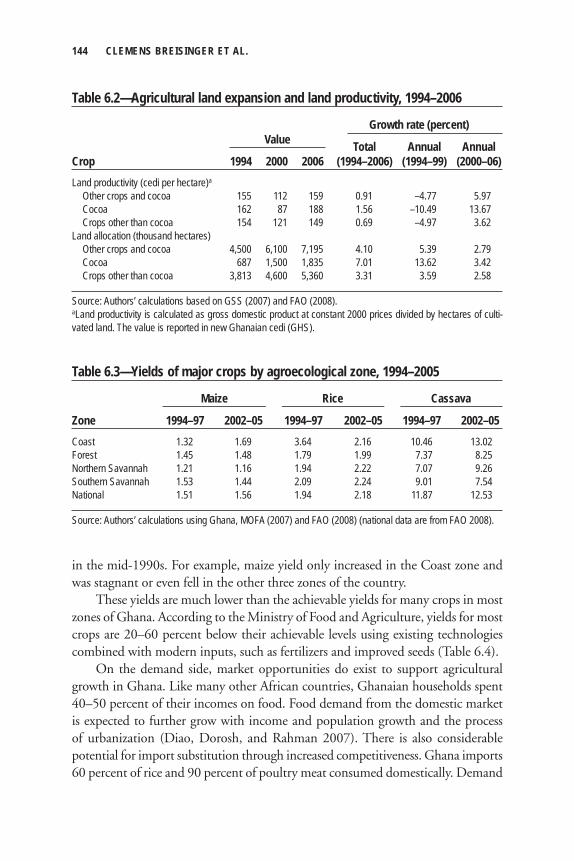
144 CLEMENS BREISINGER ET AL.
in the mid-1990s. For example, maize yield only increased in the Coast zone and was stagnant or even fell in the other three zones of the country.
These yields are much lower than the achievable yields for many crops in most zones of Ghana. According to the Ministry of Food and Agriculture, yields for most crops are 20–60 percent below their achievable levels using existing technologies combined with modern inputs, such as fertilizers and improved seeds (Table 6.4).
On the demand side, market opportunities do exist to support agricultural growth in Ghana. Like many other African countries, Ghanaian households spent 40–50 percent of their incomes on food. Food demand from the domestic market is expected to further grow with income and population growth and the process of urbanization (Diao, Dorosh, and Rahman 2007). There is also considerable potential for import substitution through increased competitiveness. Ghana imports 60 percent of rice and 90 percent of poultry meat consumed domestically. Demand
Table 6.2—Agricultural land expansion and land productivity, 1994–2006
Growth rate (percent)
Total Annual AnnualCrop 1994 2000 2006 (1994–2006) (1994–99) (2000–06)Land productivity (cedi per hectare)a Other crops and cocoa 155 112 159 0.91 –4.77 5.97 Cocoa 162 87 188 1.56 –10.49 13.67 Crops other than cocoa 154 121 149 0.69 –4.97 3.62Land allocation (thousand hectares) Other crops and cocoa 4,500 6,100 7,195 4.10 5.39 2.79 Cocoa 687 1,500 1,835 7.01 13.62 3.42 Crops other than cocoa 3,813 4,600 5,360 3.31 3.59 2.58
Source: Authors’ calculations based on GSS (2007) and FAO (2008). aLand productivity is calculated as gross domestic product at constant 2000 prices divided by hectares of culti-vated land. The value is reported in new Ghanaian cedi (GHS).
Value
Table 6.3—Yields of major crops by agroecological zone, 1994–2005
Maize Rice Cassava
Zone 1994–97 2002–05 1994–97 2002–05 1994–97 2002–05Coast 1.32 1.69 3.64 2.16 10.46 13.02Forest 1.45 1.48 1.79 1.99 7.37 8.25Northern Savannah 1.21 1.16 1.94 2.22 7.07 9.26Southern Savannah 1.53 1.44 2.09 2.24 9.01 7.54National 1.51 1.56 1.94 2.18 11.87 12.53
Source: Authors’ calculations using Ghana, MOFA (2007) and FAO (2008) (national data are from FAO 2008).
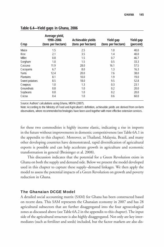
GHANA 145
for these two commodities is highly income elastic, indicating a rise in imports in the future without improvements in domestic competitiveness (see Table 6A.1 in the appendix to this chapter). Moreover, as Thailand, Malaysia, Brazil, and many other developing countries have demonstrated, rapid diversifi cation of agricultural exports is possible and can help accelerate growth in agriculture and economic transformation in general (Breisinger et al. 2008).
This discussion indicates that the potential for a Green Revolution exists in Ghana on both the supply and demand side. Below we present the model developed used in this chapter to capture these supply–demand linkages. We then apply the model to assess the potential impacts of a Green Revolution on growth and poverty reduction in Ghana.
The Ghanaian DCGE Model A detailed social accounting matrix (SAM) for Ghana has been constructed based on recent data. This SAM represents the Ghanaian economy in 2007 and has 28 agricultural subsectors that are further disaggregated into the four agroecological zones as discussed above (see Table 6A.2 in the appendix to this chapter). The input side of the agricultural structure is also highly disaggregated. Not only are key inter-mediates (such as fertilizer and seeds) included, but the factor markets are also dis-
Table 6.4—Yield gaps in Ghana, 2006
Average yield, 1990–2006 Achievable yields Yield gap Yield gapCrop (tons per hectare) (tons per hectare) (tons per hectare) (percent)Maize 1.5 2.5 1.0 40.0Rice 2.1 3.5 1.4 40.0Millet 0.8 1.5 0.7 46.7Sorghum 1.0 1.5 0.5 33.3Cassava 11.9 28.0 16.1 57.5Cocoyams 6.7 8.0 1.3 16.3Yams 12.4 20.0 7.6 38.0Plantains 8.1 10.0 1.9 19.0Sweet potatoes 8.5 18.0 9.5 52.8Cowpeas 1.0 1.3 0.3 23.1Groundnuts 0.8 1.0 0.2 20.0Soybeans 0.8 1.0 0.2 20.0Cocoa 0.4 1.0 0.6 60.0
Source: Authors’ calculations using Ghana, MOFA (2007).Note: According to the Ministry of Food and Agriculture’s definition, achievable yields are derived from on-farm observations, where recommended technologies have been used together with more effective extension services.
146 CLEMENS BREISINGER ET AL.
aggregated into agricultural family labor that is employed only in agriculture at the zonal level, unskilled labor that can move between agriculture and non-agriculture, and skilled labor employed mainly in nonagricultural sectors. Agri-cultural land can be allocated among different crops within each zone, but it cannot move across zones. The SAM captures remarkable differences in produc-tion structures between the Northern Savannah and the other zones of Ghana. Even though the Northern Savannah zone produces more than 34 percent of the country’s cereals and about 40 percent of its livestock, this zone makes the lowest contribution to agricultural exports (only 10 percent). Cocoa is the most impor-tant export crop in Ghana, but it can only be grown in the Forest and parts of the Coast zones. The limited export opportunities for the Savannah zones’ agriculture will be a challenge for these zones to benefi t from any export-oriented growth strategy discussed below.
To capture the linkages of agriculture with the rest of the economy, the SAM and the model include 32 nonagricultural sectors, many of which are agricultural processing sectors, which is consistent with Ghana’s current manufacturing struc-ture. Service sectors are also highly disaggregated to capture the sector’s market linkages with agriculture and nonagriculture through transportation, trade, and fi nancial services, which are all explicitly defi ned in the model.
The SAM fi rst aggregates consumers by rural and urban location, and then by the four agroecological zones. Households in the country’s capital city, Accra, are separated as a stand-alone group from the rest of the urban households in the Coast zone (where Accra is located) because of their very different income level and con-sumption patterns. We then further classify households according to 10 deciles that are defi ned by per capita income levels nationwide. In total, the model has 90 repre-sentative household groups. Incomes distributed across households are endogenous variables. Although rural households earn their income from factors (land, capital, and family labor) employed in agricultural production, they also participate in non-farm activities through markets for unskilled and skilled labor that are economywide factors. Urban households earn capital income and wages for skilled labor employed in nonagricultural activities and wage income for unskilled labor employed in both agricultural and nonagricultural activities. To capture growth impact on poverty, the DCGE model is further linked with a microsimulation model, which includes all sample households in the survey dataset (see Chapter 2 in this volume).
Baseline and Accelerated Growth ScenariosTwo scenarios are considered. The fi rst scenario simulates a business-as-usual situ-ation of economic development, which is called the “baseline” scenario. This sce-nario assumes that the Ghanaian economy will continue to grow along the recent trends until 2015. The second scenario models an accelerated growth path that is
GHANA 147
associated with an increase in agricultural productivity. In this scenario exogenous increases in total factor productivity (TFP) at the agricultural subsector level (crops and livestock production) are the driving forces for growth to attain achievable yields nationwide by 2015. Land expansion remains at baseline levels. In most cases we report the model results at the national level as averages, yet the model simultane-ously solves for zonal level results in the simulation. We take the different growth potentials among the four zones into consideration in designing the TFP growth rate, but unevenly distributed growth opportunities among farmers in each zone are not taken into account. For example, for farmers in areas with high agricultural poten-tial, better market access conditions, and relatively high market participation rates (such as in some areas of eastern Ghana’s Forest zone), maize yields are likely to be doubled once modern inputs are used. However, in some areas of northern Ghana with its long-term trend of land degradation, achieving a 30 percent increase in maize yields may be a challenge.
By contrasting model results of the agriculture-led growth scenario with those derived from the baseline, the transformative power of agriculture in Ghana can be assessed and analyzed. The use of the DCGE model allows for a detailed analysis of constraints, trade-offs, and linkage effects in the process, yet its results should be interpreted as a best-case scenario in which necessary investments in agricultural productivity are realized.
In the baseline scenario, land expansion is the main factor for agricultural growth, a situation consistent with recent growth patterns. Together with modest increases in productivity, agriculture grows at 4.2 percent annually in the simulated period (2007–15). Industry and services also grow according to their recent trends, at 5.6 percent and 5.2 percent per year, respectively.
The agriculture-led scenario targets higher crop yields that increase gradually over the simulated period. To identify yield targets, we choose a level of annual change in TFP coeffi cients for each individual crop across the four zones to endoge-nously obtain crop yields consistent with achievable yields by the end of the simula-tion period. These targeted yield levels are presented in Table 6.4. These targets require approximately 4.6–8.1 percent annual TFP growth for most crops. This growth in crop TFP, which combines with productivity growth in the noncrop sec-tors (mainly livestock), the endogenous accumulation of capital, and the reallocation of unskilled labor across different sectors in the economy, leads Ghana’s agricultural sector to grow at an average annual rate of 6 percent, a growth rate consistent with the Comprehensive Africa Agriculture Development Programme (CAADP) target set by the New Partnership for Africa’s Development (NEPAD). Agriculture is the largest sector in the Ghanaian economy: together with its linkage effects, accel-erating agricultural growth through productivity change results in substantial growth of the national economy: 5.8 percent total GDP growth per year compared to 4.9 percent in the baseline scenario (Table 6.5).
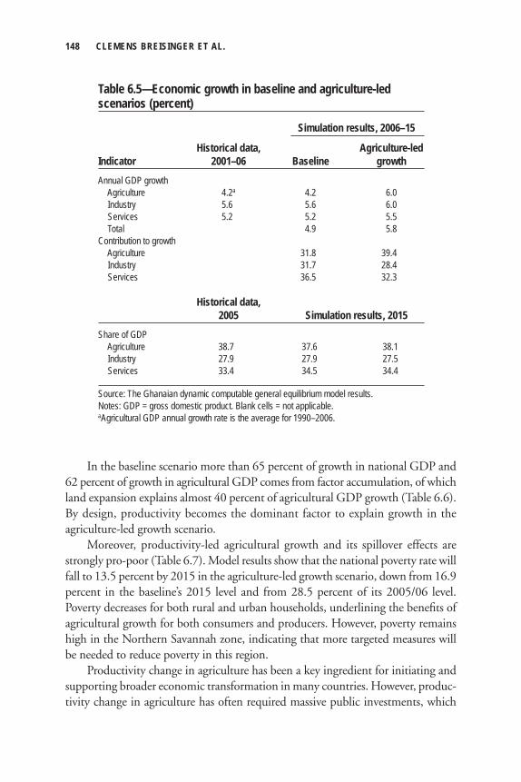
148 CLEMENS BREISINGER ET AL.
In the baseline scenario more than 65 percent of growth in national GDP and 62 percent of growth in agricultural GDP comes from factor accumulation, of which land expansion explains almost 40 percent of agricultural GDP growth (Table 6.6). By design, productivity becomes the dominant factor to explain growth in the agriculture-led growth scenario.
Moreover, productivity-led agricultural growth and its spillover effects are strongly pro-poor (Table 6.7). Model results show that the national poverty rate will fall to 13.5 percent by 2015 in the agriculture-led growth scenario, down from 16.9 percent in the baseline’s 2015 level and from 28.5 percent of its 2005/06 level. Poverty decreases for both rural and urban households, underlining the benefi ts of agricultural growth for both consumers and producers. However, poverty remains high in the Northern Savannah zone, indicating that more targeted measures will be needed to reduce poverty in this region.
Productivity change in agriculture has been a key ingredient for initiating and supporting broader economic transformation in many countries. However, produc-tivity change in agriculture has often required massive public investments, which
Table 6.5—Economic growth in baseline and agriculture-led scenarios (percent)
Simulation results, 2006–15
Historical data, Agriculture-ledIndicator 2001–06 Baseline growthAnnual GDP growth Agriculture 4.2a 4.2 6.0 Industry 5.6 5.6 6.0 Services 5.2 5.2 5.5 Total 4.9 5.8Contribution to growth Agriculture 31.8 39.4 Industry 31.7 28.4 Services 36.5 32.3
Historical data, 2005 Simulation results, 2015Share of GDP Agriculture 38.7 37.6 38.1 Industry 27.9 27.9 27.5 Services 33.4 34.5 34.4
Source: The Ghanaian dynamic computable general equilibrium model results. Notes: GDP = gross domestic product. Blank cells = not applicable. aAgricultural GDP annual growth rate is the average for 1990–2006.
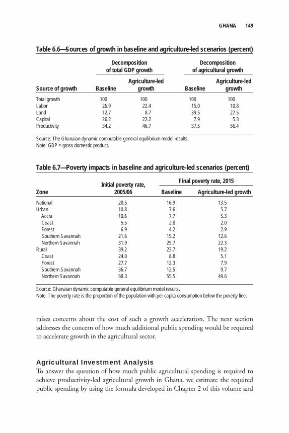
GHANA 149
raises concerns about the cost of such a growth acceleration. The next section addresses the concern of how much additional public spending would be required to accelerate growth in the agricultural sector.
Agricultural Investment AnalysisTo answer the question of how much public agricultural spending is required to achieve productivity-led agricultural growth in Ghana, we estimate the required public spending by using the formula developed in Chapter 2 of this volume and
Table 6.6—Sources of growth in baseline and agriculture-led scenarios (percent)
Decomposition Decomposition of total GDP growth of agricultural growth
Agriculture-led Agriculture-ledSource of growth Baseline growth Baseline growthTotal growth 100 100 100 100Labor 26.9 22.4 15.0 10.8Land 12.7 8.7 39.5 27.5Capital 26.2 22.2 7.9 5.3Productivity 34.2 46.7 37.5 56.4
Source: The Ghanaian dynamic computable general equilibrium model results.Note: GDP = gross domestic product.
Table 6.7—Poverty impacts in baseline and agriculture-led scenarios (percent)
Initial poverty rate, Zone 2005/06 Baseline Agriculture-led growthNational 28.5 16.9 13.5Urban 10.8 7.6 5.7 Accra 10.6 7.7 5.3 Coast 5.5 2.8 2.0 Forest 6.9 4.2 2.9 Southern Savannah 21.6 15.2 12.6 Northern Savannah 31.9 25.7 22.3Rural 39.2 23.7 19.2 Coast 24.0 8.8 5.1 Forest 27.7 12.3 7.9 Southern Savannah 36.7 12.5 9.7 Northern Savannah 68.3 55.5 49.6
Source: Ghanaian dynamic computable general equilibrium model results. Note: The poverty rate is the proportion of the population with per capita consumption below the poverty line.
Final poverty rate, 2015
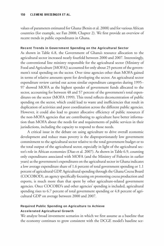
150 CLEMENS BREISINGER ET AL.
values of parameters estimated for Ghana (Benin et al. 2008) and for various African countries (for example, see Fan 2008; Chapter 2). We fi rst provide an overview of recent trends in public expenditures in Ghana.
Recent Trends in Government Spending on the Agricultural SectorAs shown in Table 6.8, the Government of Ghana’s resource allocation to the agricultural sector increased nearly fourfold between 2000 and 2007. Interestingly, the conventional line ministry responsible for the agricultural sector (Ministry of Food and Agriculture [MOFA]) accounted for only about 25 percent of the govern-ment’s total spending on the sector. Over time agencies other than MOFA gained in terms of relative amounts spent for developing the sector. An agricultural sector expenditure review carried out across similar expenditure categories during 1995–97 showed MOFA as the highest spender of government funds allocated to the sector, accounting for between 48 and 57 percent of the government’s total expen-ditures on the sector (MOFA 1999). This trend refl ects deconcentration of public spending on the sector, which could lead to waste and ineffi ciencies that result in duplication of activities and poor coordination across the different public agencies. However, it could also lead to greater allocative effi ciency of public resources if the non-MOFA agencies that are contributing to agriculture have better informa-tion than MOFA about the needs for and requirements of public services in their jurisdictions, including the capacity to respond to those needs.
A critical issue in the debate on using agriculture to drive overall economic development and reduce mass poverty is the disproportionately low government commitment to the agricultural sector relative to the total government budget or to the total output of the agricultural sector, especially in light of the agricultural sec-tor’s role in African economies (Diao et al. 2007). As shown in Table 6.9, counting only expenditures associated with MOFA (and the Ministry of Fisheries in earlier years) as the government’s expenditures on the agricultural sector in Ghana indicates a low average expenditure share of 1.6 percent of total government spending or 1.1 percent of agricultural GDP. Agricultural spending through the Ghana Cocoa Board (COCOBOD), an agency specifi cally focusing on promoting cocoa production and exports, is much more than that spent by other agriculture-related government agencies. Once COCOBD’s and other agencies’ spending is included, agricultural spending rises to 6.7 percent of total government spending or 4.8 percent of agri-cultural GDP on average between 2000 and 2007.
Required Public Spending on Agriculture to Achieve Accelerated Agricultural Growth We analyze broad investment scenarios in which we fi rst assume as a baseline that the economy continues to grow consistent with the DCGE model’s baseline sce-
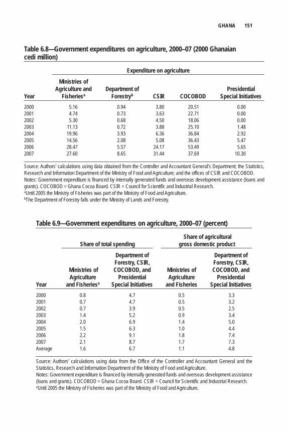
GHANA 151
Table 6.8—Government expenditures on agriculture, 2000–07 (2000 Ghanaian cedi million)
Expenditure on agriculture
Ministries of Agriculture and Department of Presidential Year Fisheriesa Forestryb CSIR COCOBOD Special Initiatives2000 5.16 0.94 3.80 20.51 0.002001 4.74 0.73 3.63 22.71 0.002002 5.30 0.68 4.50 18.06 0.002003 11.13 0.72 3.88 25.10 1.482004 19.96 3.93 6.36 36.84 2.922005 14.56 2.08 5.08 36.43 5.472006 28.47 5.57 24.17 53.49 5.652007 27.60 8.65 31.44 37.69 10.30
Source: Authors’ calculations using data obtained from the Controller and Accountant General’s Department; the Statistics, Research and Information Department of the Ministry of Food and Agriculture; and the offices of CSIR and COCOBOD.Notes: Government expenditure is financed by internally generated funds and overseas development assistance (loans and grants). COCOBOD = Ghana Cocoa Board. CSIR = Council for Scientific and Industrial Research.aUntil 2005 the Ministry of Fisheries was part of the Ministry of Food and Agriculture. bThe Department of Forestry falls under the Ministry of Lands and Forestry.
Table 6.9—Government expenditures on agriculture, 2000–07 (percent)
Share of agricultural Share of total spending gross domestic product
Department of Department of Forestry, CSIR, Forestry, CSIR, Ministries of COCOBOD, and Ministries of COCOBOD, and Agriculture Presidential Agriculture PresidentialYear and Fisheriesa Special Initiatives and Fisheries Special Initiatives2000 0.8 4.7 0.5 3.32001 0.7 4.7 0.5 3.22002 0.7 3.9 0.5 2.52003 1.4 5.2 0.9 3.42004 2.0 6.9 1.4 5.02005 1.5 6.3 1.0 4.42006 2.2 9.1 1.8 7.42007 2.1 8.7 1.7 7.3Average 1.6 6.7 1.1 4.8
Source: Authors’ calculations using data from the Office of the Controller and Accountant General and the Statistics, Research and Information Department of the Ministry of Food and Agriculture.Notes: Government expenditure is financed by internally generated funds and overseas development assistance (loans and grants). COCOBOD = Ghana Cocoa Board. CSIR = Council for Scientific and Industrial Research.aUntil 2005 the Ministry of Fisheries was part of the Ministry of Food and Agriculture.
152 CLEMENS BREISINGER ET AL.
nario. We further assume that total public spending in the baseline scenario contin-ues to grow at the 2000–07 average of 11.6 percent per year and that the share of public agricultural spending of total spending is maintained at an average of 6.7 percent per year (see Table 6.10). We then analyze four investment scenarios to simulate public agricultural spending required to achieve the agricultural growth targeted in the agriculture-led growth scenario from the DCGE model. The sce-narios vary according to the assumptions about the sources of agricultural growth deriving from different types of public spending in agriculture and rural areas. The fi rst scenario (Scenario I) assumes that the agricultural growth-rate gap of 1.8 per-centage points (6.0 percent in the agriculture-led growth scenario minus 4.2 percent in the baseline) is driven by raising public agricultural spending only. That is, public spending on the nonagricultural sector continues to grow as in the baseline scenario. Also, other factors (for example, interaction effects among different types of spend-ing, crowding effects of public spending on private spending, and growth in non-spending factors that affect agricultural productivity and its effects) remain unchanged. The second scenario (Scenario II) analyzes the implications of raising the profi le of agricultural development spending, assuming an equal (50:50) split with recurrent spending.
The third scenario (Scenario III) assumes that public spending on the non-agricultural sector grows by an additional 1.14 percentage points per year to close the nonagricultural sector growth-rate gap of 0.4 percentage points (that is, the target of 5.7 percent minus baseline of 5.3 percent).1 This scenario further assumes that public spending on each of the nonagricultural sectors (education, health, roads, and so on) grows at the same rate to maintain their current shares in total nonagricultural spending. The fourth scenario (Scenario IV) is similar to the previ-ous one except that it assumes that public spending on the different nonagricultural sectors grows at different rates to take advantage of those with greater estimated returns to spending. The motivation for this scenario is similar to that for Scenario II: to analyze the implication of raising the profi le of public spending on rural infrastructure, which the evidence shows has a much larger positive and signifi cant impact on agricultural productivity than do other interventions (for example, see Fan 2008). We adjust the shares to equal the marginal returns.
In each of the investment scenarios we simulate the public agricultural spending requirement under three assumptions regarding the effi ciency of public spend-ing (low, medium, and high) based on estimated elasticities from the literature. First, we constructed lower and upper limits of a 90 percent confi dence interval around the point estimates. The minimum value of the lower limits and maximum value of the upper limits were chosen as the low and high effi ciency elasticities, respec-tively. Then, the midpoint of the low and high effi ciency elasticities was chosen as the medium effi ciency elasticity. For the elasticities with respect to nonagricultural
GHANA 153
public spending, we use a weighted average for education, health, and feeder roads, where the weights are the expenditure shares. See Table 6A.3 in the appendix to this chapter for details on the assumed values of key parameters used in the simulations. We use 2007 as the starting point for the simulations, which are run for the 2007–15 period. All simulated monetary values are in 2007 constant prices.
We have made simple assumptions to carry out the simulation exercise within the framework described in Chapter 2. The limitations of the formula discussed there also apply here. Against this cautionary background, we now present the simu-lation results: the spending requirements for the baseline and those for Scenarios I–IV. The parameter values used in public investment simulations are summarized in Table 6A.4 in the appendix to this chapter. The results from the investment analy-sis are shown in Table 6.10.
Investment Analysis Results: Baseline ScenarioIn the baseline scenario (that is, maintaining the status quo), total government agricultural spending from 2007 to 2015 would be 3,837 million Ghanaian cedi (GHS), which represents about GHS426 million per year. Although the share of government agricultural spending in total government spending is maintained at 6.7 percent per year by design, the agricultural spending as a share of agricultural GDP will rise from 5.6 percent in 2007 to 9.4 percent in 2015. This is because government agricultural spending grows faster (11.6 percent per year) than agricul-tural GDP (4.2 percent per year).
Investment Analysis Results: Scenario IScenario I simulates agriculture expenditure requirements assuming that the source of additional agricultural GDP growth is derived from increasing public agricultural spending only. Although it is unrealistic to expect public agricultural spending to be the only source of additional growth, the requirements that follow can be inter-preted as the total (public and private) maximum resources and investments needed to generate the additional growth, assuming similar across-the-board spending effi ciencies. The simulation results show that this requires the annual growth rate in agricultural spending to increase from the baseline value of 11.6 to 58.9, 40.7, and 32.6 percent per year in the low, midpoint, and high effi ciency spending sce-narios, respectively. The total government budget in these respective spending effi ciency scenarios is estimated to grow at 22.3, 16.0, and 14.1 percent per year.
With agricultural spending thus growing more rapidly than total spending, the share of agricultural spending in total expenditures will rise from the baseline value of 6.7 percent per year to annual average values of 34.1, 20.0, and 15.0 percent in the three spending effi ciency scenarios, respectively. The share of agricultural spend-ing in agricultural GDP will rise from the baseline value of 5.6 percent to 50.3, 23.6,
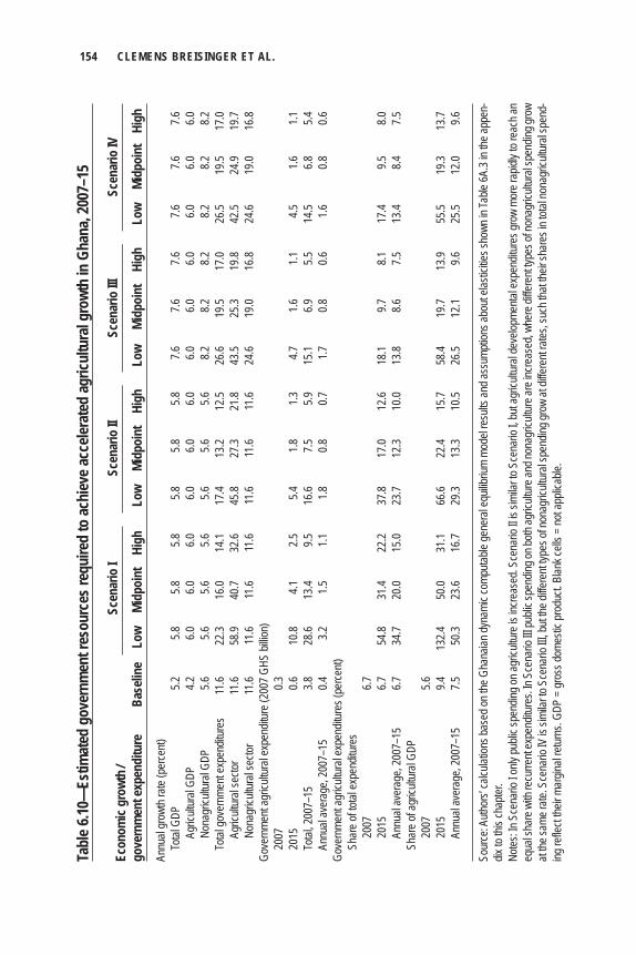
154 CLEMENS BREISINGER ET AL.
Tabl
e 6.10
—Es
timat
ed g
over
nmen
t res
ourc
es re
quire
d to
achi
eve a
ccele
rate
d ag
ricul
tura
l gro
wth
in G
hana
, 200
7–15
Econ
omic
grow
th /
Scen
ario
I Sc
enar
io II
Scen
ario
III
Scen
ario
IV
gove
rnm
ent e
xpen
ditu
re
Base
line
Low
Midp
oint
Hi
gh
Low
Midp
oint
Hi
gh
Low
Midp
oint
Hi
gh
Low
Midp
oint
Hi
ghAn
nual
grow
th ra
te (p
erce
nt)
Total
GDP
5.2
5.8
5.8
5.8
5.8
5.8
5.8
7.6
7.6
7.6
7.6
7.6
7.6
Agric
ultur
al GD
P 4.2
6.0
6.0
6.0
6.0
6.0
6.0
6.0
6.0
6.0
6.0
6.0
6.0
Nona
gricu
ltura
l GDP
5.6
5.6
5.6
5.6
5.6
5.6
5.6
8.2
8.2
8.2
8.2
8.2
8.2
To
tal go
vern
ment
expe
nditu
res
11.6
22.3
16.0
14.1
17.4
13.2
12.5
26.6
19.5
17.0
26.5
19.5
17.0
Agric
ultur
al se
ctor
11.6
58.9
40.7
32.6
45.8
27.3
21.8
43.5
25.3
19.8
42.5
24.9
19.7
Nona
gricu
ltura
l sec
tor
11.6
11.6
11.6
11.6
11.6
11.6
11.6
24.6
19.0
16.8
24.6
19.0
16.8
Gove
rnme
nt ag
ricult
ural
expe
nditu
re (2
007 G
HS bi
llion)
20
07
0.3
2015
0.6
10
.8 4.1
2.5
5.4
1.8
1.3
4.7
1.6
1.1
4.5
1.6
1.1
To
tal, 2
007–
15
3.8
28.6
13.4
9.5
16.6
7.5
5.9
15.1
6.9
5.5
14.5
6.8
5.4
Annu
al av
erag
e, 20
07–1
5 0.4
3.2
1.5
1.1
1.8
0.8
0.7
1.7
0.8
0.6
1.6
0.8
0.6
Gove
rnme
nt ag
ricult
ural
expe
nditu
res (
perce
nt)
Shar
e of to
tal ex
pend
iture
s
20
07
6.7
20
15
6.7
54.8
31.4
22.2
37.8
17.0
12.6
18.1
9.7
8.1
17.4
9.5
8.0
An
nual
aver
age,
2007
–15
6.7
34.7
20.0
15.0
23.7
12.3
10.0
13.8
8.6
7.5
13.4
8.4
7.5
Shar
e of a
gricu
ltura
l GDP
20
07
5.6
20
15
9.4
132.4
50
.0 31
.1 66
.6 22
.4 15
.7 58
.4 19
.7 13
.9 55
.5 19
.3 13
.7
An
nual
aver
age,
2007
–15
7.5
50.3
23.6
16.7
29.3
13.3
10.5
26.5
12.1
9.6
25.5
12.0
9.6
Sour
ce: A
uthor
s’ ca
lculat
ions b
ased
on th
e Gha
naian
dyna
mic c
ompu
table
gene
ral e
quilib
rium
mode
l resu
lts an
d ass
umpti
ons a
bout
elasti
cities
show
n in T
able
6A.3
in the
appe
n-dix
to th
is ch
apter
.No
tes: In
Sce
nario
I only
publi
c spe
nding
on ag
ricult
ure i
s inc
reas
ed. S
cena
rio II
is sim
ilar t
o Sce
nario
I, bu
t agr
icultu
ral d
evelo
pmen
tal ex
pend
iture
s gro
w mo
re ra
pidly
to re
ach a
n eq
ual s
hare
with
recu
rrent
expe
nditu
res.
In Sc
enar
io III
publi
c spe
nding
on bo
th ag
ricult
ure a
nd no
nagr
icultu
re ar
e inc
reas
ed, w
here
diffe
rent
types
of no
nagr
icultu
ral s
pend
ing gr
ow
at the
same
rate.
Sce
nario
IV is
simi
lar to
Sce
nario
III, b
ut the
diffe
rent
types
of no
nagr
icultu
ral s
pend
ing gr
ow at
diffe
rent
rates
, suc
h tha
t their
shar
es in
total
nona
gricu
ltura
l spe
nd-
ing re
flect
their m
argin
al re
turns
. GDP
= gr
oss d
omes
tic pr
oduc
t. Blan
k cell
s = no
t app
licab
le.
GHANA 155
and 16.7 percent per year. These values translate into additional (that is, in addition to the baseline values) spending on the agricultural sector by a total amount of about GHS5,632 million–24,725 million during 2007–15, or GHS704 million–3,091 million per year. The low and high end values correspond to the high and low spend-ing effi ciency scenarios, respectively. These ranges are rather large, which is due to the sensitivity of the elasticities and the wide range of the elasticities used—the high value is nearly three times as large as the low value. Nevertheless, these results mean that the political and institutional context of public spending programs in Ghana will be critical in determining the resource requirements. Going by the assumed midpoint value of the elasticity used, for example (0.086), the total agricultural budget from 2007 to 2015 required to achieve an agricultural GDP growth rate of 6 percent per year would be about GHS9,550 million (or GHS1,194 million per year).
Investment Analysis Results: Scenario IIContinuing to assume that the source of additional growth is derived solely from increasing agricultural expenditures, the cost requirements are much lower when the share of development expenditure is raised to 50 percent (see Table 6.10 and Figure 6.1). The shares of agricultural spending in total expenditures are now 23.2, 12.3, and 10.0 percent in the three spending effi ciency scenarios, respectively. These translate into additional spending (that is, in addition to the baseline values) on the agricultural sector by a total amount of about GHS2,100–12,790 million during 2007–15 or GHS263–1,599 million per year, less than 50 percent of the cost requirements in Scenario I.
Investment Analysis Results: Scenario IIIIn Scenario III public spending on the nonagricultural sector is also increased, but the rate of increase is the same across all nonagricultural subsectors. Because spend-ing on the nonagricultural sector has an effect on agricultural productivity growth (with an assumed elasticity of 0.01–0.09), the simulated resource requirements for the agricultural sector are lower than in Scenario II, although the overall budgetary resources are higher.
The simulation results of Scenario III in Table 6.10 show that the average annual growth rate in public agricultural expenditure would be 43.5, 25.3, and 19.8 percent in the low, midpoint, and high effi ciency spending scenarios, respectively (which is about 2–3 percentage points lower than the respective growth rates in Scenario II). The total government budget in the respective spending effi ciency scenarios is now estimated to grow at 26.6, 19.5, and 17.0 percent per year. The share of agriculture in total expenditure will be 13.8, 8.6, and 7.5 percent in the three spending effi ciency scenarios, respectively, while the share of agricultural spending in agricultural GDP will be 26.5, 12.1, and 9.6 percent per year. These
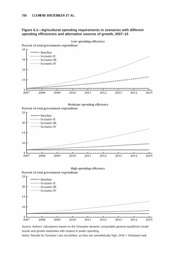
156 CLEMENS BREISINGER ET AL.
BaselineScenario IIScenario IIIScenario IV
Percent of total government expenditureLow spending efficiency
45
5
35
25
15
201520142013201220112010200920082007
BaselineScenario IIScenario IIIScenario IV
Percent of total government expenditureModerate spending efficiency
25
5
20
15
10
201520142013201220112010200920082007
BaselineScenario IIScenario IIIScenario IV
Percent of total government expenditureHigh spending efficiency
25
5
20
15
10
201520142013201220112010200920082007
Figure 6.1—Agricultural spending requirements in scenarios with different spending efficiencies and alternative sources of growth, 2007–15
Source: Authors’ calculations based on the Ghanaian dynamic computable general equilibrium model results and growth elasticities with respect to public spending.Notes: Results for Scenario I are not plotted, as they are unrealistically high. GHS = Ghanaian cedi.
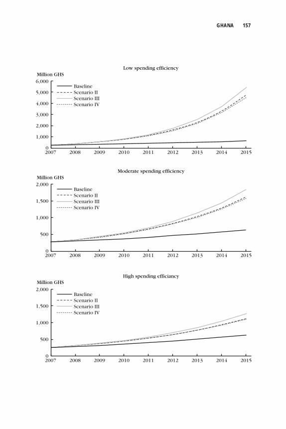
GHANA 157
BaselineScenario IIScenario IIIScenario IV
Million GHSLow spending efficiency
6,000
5,000
0
4,000
3,000
1,000
2,000
201520142013201220112010200920082007
201520142013201220112010200920082007
201520142013201220112010200920082007
BaselineScenario IIScenario IIIScenario IV
Million GHSModerate spending efficiency
2,000
0
1,500
1,000
500
BaselineScenario IIScenario IIIScenario IV
Million GHSHigh spending efficiancy
2,000
0
1,500
1,000
500
158 CLEMENS BREISINGER ET AL.
numbers translate into additional (that is, over the baseline values) spending on the agricultural sector by a total amount of about GHS1,627–1,216 million over 2007–15, or GHS203–1,402 million per year. Again, the low- and high-end values correspond to the high and low spending effi ciency scenarios, respectively. Comparing the resource requirements in Scenarios II and III shows little difference, refl ecting the small effect of overall growth in public nonagricultural spending on agricultural growth. The literature shows that the effect of public nonagricultural spending on agricultural productivity is mainly from spending on rural infrastructure, particularly on rural roads. However, the share of government spending on rural infrastructure in general and rural roads in particular in Ghana is very small. Therefore, increasing spending on different types of nonagricultural public goods and services at equal rates is not likely to be prudent.
Investment Analysis Results: Scenario IVThe idea of shifting or increasing resources in favor of sectors, subsectors, or activities that contribute most to a development objective is the motivation for Scenario IV. In contrast to the previous scenario, Scenario IV has different rates of increase of public nonagricultural spending for the different sectors, so that their share in total nonagricultural spending refl ects their marginal returns. The simulation results show that the average annual growth rate in public agricultural spending would be 42.5, 24.9, and 19.7 percent in the low, midpoint, and high effi ciency spending scenarios, respectively (which is about 0.9, 0.4, and 0.1 percentage points lower than the respec-tive growth rates in Scenario III). The total government budget in the respective spending effi ciency scenarios grows at a lower rate (about 0.5 percent lower than in Scenario III) and now is estimated to grow at 26.5, 19.5, and 17.0 percent per year.
The share of agricultural spending in total expenditures will now be 13.4, 8.4, and 7.5 percent in the three spending effi ciency scenarios, respectively, and the share of agricultural spending in agricultural GDP will be 25.5, 12.0, and 9.6 percent per year. Using the midpoint values of the elasticities, the total spending on the agricul-tural sector from 2007 to 2015 required to achieve the accelerated agricultural growth would be about GHS2,958 million (or GHS370 million per year), which is about 4 percent lower than the estimated requirements in Scenario III. Therefore, shifting or increasing public resources in favor of sectors, subsectors, or activities that contribute most to raising agricultural productivity growth and overall growth will be important.
Implications of Our Assumptions for Simulated Expenditure Requirements Given that agricultural production in Ghana is considered a private sector activity, a key policy issue is how much the private sector should contribute toward the
GHANA 159
resource gap. Although providing actual numbers on private sector investments is outside the scope of this research, here we discuss the implications of changing some of the underlying assumptions made in simulating the expenditure requirements. We focus on implications of policies and public spending decisions on the simulated expenditure requirements vis-à-vis their effects on private sector investments. We also discuss other effects, including improving use and effi ciency of agricultural inputs and interactions among different types of public expenditures.
Regarding the public–private spending interface (that is, the idea that public plus private spending is arguably a zero-sum game in the sense that government spending is fi nanced by taxation of private investment), external sources of funding (both loans and grants) make up about 35 percent of the Government of Ghana’s total budget expenditure (Quartey 2005). Thus, the zero-sum game argument is very important for Ghana, and how the crowding-out or crowding-in effects operate in the future will be critical for determining the total resources required to achieve the agricultural growth targets, as well as for the necessary contribution by the pri-vate sector. Thus, policies and public spending decisions that encourage private investment in farm capital will be very important. Similarly, policies and public spending that help improve use and effi ciency of agricultural inputs will also be critical for raising overall agricultural productivity, reducing total resource require-ments and both public and private contributions.
Interactions (complementarity or substitution effects) among different types of public spending also matter for the cost calculations. The interaction effects between agricultural expenditures and each of the nonagricultural sectors (education, health, and rural roads) were implicitly taken into account in the simulations and were incorporated into the assumed elasticities. Ministries, departments, and agencies of the different sectors may view others as competitors for national budget expendi-tures (another zero-sum game), which should not be the case to the extent that spending on one sector affects the performance of other sectors. Thus, policies that promote cross-sectoral programs leading to joint outcomes that are more than the sum of individual outcomes will also be important for raising overall agricultural productivity.
Conclusions Impressive growth and poverty reduction over the past 20 years have made Ghana an African success story. Agricultural growth has played an important role in this effort. However, agricultural growth in Ghana has been mainly driven by area expansion as opposed to a Green Revolution of the sort experienced by many Asian countries, in which growth is driven by productivity. Potential for such productivity-led growth exists in Ghana, exemplifi ed by signifi cant gaps between current and
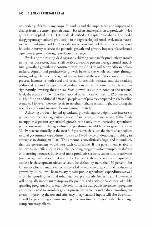
160 CLEMENS BREISINGER ET AL.
achievable yields for many crops. To understand the importance and impacts of a change from the current growth pattern based on land expansion to productivity-led growth, we applied the DCGE model described in Chapter 2 to Ghana. The model disaggregates agricultural production to the agroecological zonal level, and a macro- to microsimulation model includes all sample households of the most recent national household survey to assess the potential growth and poverty impacts of accelerated agricultural growth through productivity change.
By closing the existing yield gaps and achieving comparable productivity growth in the livestock sector, Ghana will be able to reach 6 percent average annual agricul-tural growth, a growth rate consistent with the CAADP goal set by African policy-makers. Agricultural productivity growth benefi ts the whole economy through strong linkages between the agricultural sectors and the rest of the economy. In this process, incomes of both rural and urban households increase, and the resulting additional demand for agricultural products can be met by domestic supply without signifi cantly lowering their prices. Such growth is also pro-poor. At the national level, the scenario shows that the national poverty rate will fall to 12.5 percent by 2015, lifting an additional 850,000 people out of poverty compared to the baseline scenario. However, poverty levels in northern Ghana remain high, indicating the need for additional measures beyond growth strategy.
Achieving productivity-led agricultural growth requires a signifi cant increase in public investments in agriculture, rural infrastructure, and marketing. If the funds to support 6 percent agricultural growth come only from increasing agricultural public investment, the agricultural expenditures would have to grow by about 32–59 percent annually in the next 5–8 years, which causes the share of agriculture in total government expenditures to rise to 15–34 percent, doubling or trebling its average share during 2000–07. This amount is unrealistically large, and it is unlikely that the government would bear such costs alone. If the government is able to achieve greater effi ciency in its public spending programs—for example, by shifting or increasing resources in favor of more productive sectors, subsectors, or activities (such as agricultural or rural roads development), then the resources required to achieve its development objective could be slashed by more than 50 percent. For Ghana to achieve a middle-income status led by accelerated agricultural productivity growth by 2015, it will be necessary to raise public agricultural expenditures as well as public spending on rural infrastructure, particularly feeder roads. However, it will be equally important to improve the political and institutional context of public spending programs by, for example, reforming the way public investment programs are implemented to crowd-in greater private investments and reduce crowding-out effects. Improving the use and effi ciency of agricultural inputs will also be critical, as will be promoting cross-sectoral public investment programs that have large complementary effects.
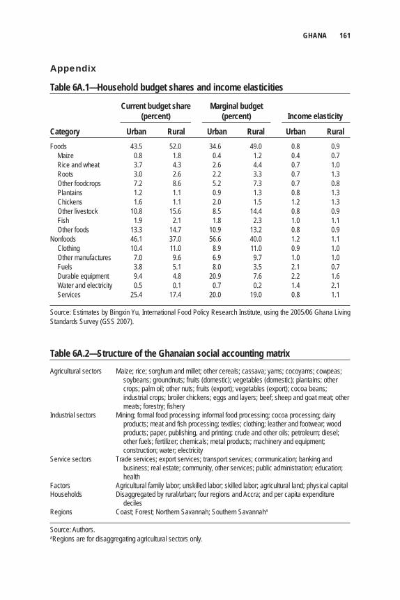
GHANA 161
Appendix
Table 6A.1—Household budget shares and income elasticities
Current budget share Marginal budget (percent) (percent) Income elasticity
Category Urban Rural Urban Rural Urban RuralFoods 43.5 52.0 34.6 49.0 0.8 0.9 Maize 0.8 1.8 0.4 1.2 0.4 0.7 Rice and wheat 3.7 4.3 2.6 4.4 0.7 1.0 Roots 3.0 2.6 2.2 3.3 0.7 1.3 Other foodcrops 7.2 8.6 5.2 7.3 0.7 0.8 Plantains 1.2 1.1 0.9 1.3 0.8 1.3 Chickens 1.6 1.1 2.0 1.5 1.2 1.3 Other livestock 10.8 15.6 8.5 14.4 0.8 0.9 Fish 1.9 2.1 1.8 2.3 1.0 1.1 Other foods 13.3 14.7 10.9 13.2 0.8 0.9Nonfoods 46.1 37.0 56.6 40.0 1.2 1.1 Clothing 10.4 11.0 8.9 11.0 0.9 1.0 Other manufactures 7.0 9.6 6.9 9.7 1.0 1.0 Fuels 3.8 5.1 8.0 3.5 2.1 0.7 Durable equipment 9.4 4.8 20.9 7.6 2.2 1.6 Water and electricity 0.5 0.1 0.7 0.2 1.4 2.1 Services 25.4 17.4 20.0 19.0 0.8 1.1
Source: Estimates by Bingxin Yu, International Food Policy Research Institute, using the 2005/06 Ghana Living Standards Survey (GSS 2007).
Table 6A.2—Structure of the Ghanaian social accounting matrixAgricultural sectors Maize; rice; sorghum and millet; other cereals; cassava; yams; cocoyams; cowpeas; soybeans; groundnuts; fruits (domestic); vegetables (domestic); plantains; other
crops; palm oil; other nuts; fruits (export); vegetables (export); cocoa beans; industrial crops; broiler chickens; eggs and layers; beef; sheep and goat meat; other meats; forestry; fishery
Industrial sectors Mining; formal food processing; informal food processing; cocoa processing; dairy products; meat and fish processing; textiles; clothing; leather and footwear; wood
products; paper, publishing, and printing; crude and other oils; petroleum; diesel; other fuels; fertilizer; chemicals; metal products; machinery and equipment; construction; water; electricity
Service sectors Trade services; export services; transport services; communication; banking and business; real estate; community, other services; public administration; education;
healthFactors Agricultural family labor; unskilled labor; skilled labor; agricultural land; physical capitalHouseholds Disaggregated by rural/urban; four regions and Accra; and per capita expenditure decilesRegions Coast; Forest; Northern Savannah; Southern Savannaha
Source: Authors.aRegions are for disaggregating agricultural sectors only.
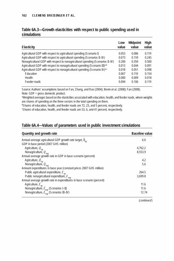
162 CLEMENS BREISINGER ET AL.
Table 6A.3—Growth elasticities with respect to public spending used in simulations
Low Midpoint HighElasticity value value valueAgricultural GDP with respect to agricultural spending (Scenario I) 0.053 0.086 0.119Agricultural GDP with respect to agricultural spending (Scenarios II–IV) 0.073 0.159 0.245Nonagricultural GDP with respect to nonagricultural spending (Scenarios II–IV) 0.200 0.350 0.500Agricultural GDP with respect to nonagricultural spending (Scenario III)a,b 0.013 0.044 0.091Agricultural GDP with respect to nonagricultural spending (Scenario IV)a,c 0.018 0.051 0.098 Education 0.067 0.110 0.154 Health 0.000 0.009 0.018 Feeder roads 0.094 0.106 0.119
Source: Authors’ assumptions based on Fan, Zhang, and Rao (2004); Benin et al. (2008); Fan (2008).Note: GDP = gross domestic product. aWeighted averages based on the elasticities associated with education, health, and feeder roads, where weights are shares of spending on the three sectors in the total spending on them. bShares of education, health, and feeder roads are 72, 23, and 5 percent, respectively.cShares of education, health, and feeder roads are 53, 6, and 41 percent, respectively.
Table 6A.4—Values of parameters used in public investment simulations
Quantity and growth rate Baseline valueAnnual average agricultural GDP growth rate target, θag 6.0GDP in base period (2007 GHS million) Agriculture, Qag 4,762.2 Nonagriculture, Qnag 8,553.9Annual average growth rate in GDP in base scenario (percent) Agriculture, Qag 4.2 Nonagriculture, Qnag 5.6Amount expenditures in base year (constant prices 2007 GHS million) Public agricultural expenditure, Eag 264.5 Public nonagricultural expenditure, Enag 3,699.8Annual average growth rate in expenditures in base scenario (percent) Agriculture, Eag 11.6 Nonagriculture, Enag (Scenarios I–II) 11.6 Nonagriculture, Enag (Scenarios III–IV) 12.74
(continued )
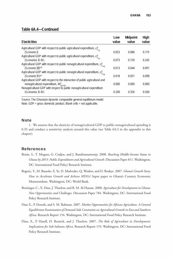
GHANA 163
Note 1. We assume that the elasticity of nonagricultural GDP to public nonagricultural spending is 0.35 and conduct a sensitivity analysis around this value (see Table 6A.3 in the appendix to this chapter).
ReferencesBenin, S., T. Mogues, G. Cudjoe, and J. Randriamamonjy. 2008. Reaching Middle-Income Status in
Ghana by 2015: Public Expenditures and Agricultural Growth. Discussion Paper 811. Washington,
DC: International Food Policy Research Institute.
Bogetic, Y., M. Bussolo, X. Ye, D. Medvedev, Q. Wodon, and D. Boakye. 2007. Ghana’s Growth Story:
How to Accelerate Growth and Achieve MDGs? Input paper to Ghana’s Country Economic
Memorandum. Washington, DC: World Bank.
Breisinger, C., X. Diao, J. Thurlow, and R. M. Al-Hassan. 2008. Agriculture for Development in Ghana:
New Opportunities and Challenges. Discussion Paper 784. Washington, DC: International Food
Policy Research Institute.
Diao X., P. Dorosh, and S. M. Rahman. 2007. Market Opportunities for African Agriculture. A General
Equilibrium Examination of Demand-Side Constraints on Agricultural Growth in East and Southern
Africa. Research Report 154. Washington, DC: International Food Policy Research Institute.
Diao, X., P. Hazell, D. Resnick, and J. Thurlow. 2007. The Role of Agriculture in Development:
Implications for Sub-Saharan Africa. Research Report 153. Washington, DC: International Food
Policy Research Institute.
Table 6A.4—Continued
Low Midpoint HighElasticities value value valueAgricultural GDP with respect to public agricultural expenditure, εQ
Eag
(Scenario I) 0.053 0.086 0.119Agricultural GDP with respect to public agricultural expenditure, εQ
Eag
(Scenarios II–IV) 0.073 0.159 0.245Agricultural GDP with respect to public nonagricultural expenditure, εQ
Enag (Scenario III)a,b 0.013 0.044 0.091Agricultural GDP with respect to public nonagricultural expenditure, εQ
Enag
(Scenario IV)a,c 0.018 0.051 0.098Agricultural GDP with respect to the interaction of public agricultural and nonagricultural expenditure, ΦQ
ag,nag 0.000 0.000 0.000Nonagricultural GDP with respect to public nonagricultural expenditure (Scenarios II–IV) 0.200 0.350 0.500
Source: The Ghanaian dynamic computable general equilibrium model. Note: GDP = gross domestic product. Blank cells = not applicable.
164 CLEMENS BREISINGER ET AL.
Fan, S., ed. 2008. Public Expenditures, Growth, and Poverty: Lessons from Developing Countries. Baltimore:
Johns Hopkins University Press.
Fan, S., X. Zhang, and N. Rao. 2004. Public Expenditure, Growth and Poverty Reduction in Rural
Uganda. Development Strategy and Governance Division Discussion Paper 4. Washington, DC:
International Food Policy Research Institute.
FAO (Food and Agriculture Organization of the United Nations). 2008. “Soaring Food Prices: Facts,
Perspectives, Impacts and Actions Required.” Paper presented at the High-Level Conference on
World Food Security: The Challenges of Climate Change and Bioenergy, Rome, June 3–5.
Freedom House. 2008. Freedom of the World 2008. Washington, DC.
Ghana, MOFA (Ministry of Food and Agriculture). 1999. “Agricultural Sector Expenditure Review,
1995–1997.” Mimeo. Accra, Ghana.
———. 2007. “District Level Agricultural Production and Price Data.” Unpublished dataset. Statistics
Research and Information Directorate, Accra, Ghana.
GSS (Ghana Statistical Service). 2007. “Ghana Living Standards Survey: Report of the Fifth Round
(GLSS 5).” Accessed January 6, 2012. www.statsghana.gov.gh/docfi les/glss5_report.pdf.
Kaufmann, D., A. Kraay, and M. Mastruzzi. 2009. Governance Matters VIII: Aggregate and Individual
Governance Indicators 1996–2008. Washington, DC: World Bank.
Quartey, P. 2005. “Innovative Ways of Making Aid Effective in Ghana: Tied Aid versus Direct Budgetary
Support.” Journal of International Development 17: 1077–1092.
World Bank. 2007. World Development Indicators. Washington, DC.
C h a p t e r 7
RwandaXinshen Diao, Shenggen Fan,
Sam Kanyarukiga, and Bingxin Yu
Despite a remarkable transition to peace and development over the past 10 years, Rwanda is still marked by the consequences of the 1994 genocide. Gross domestic product (GDP) growth averaged 7.3 percent per year
between 1995 and 2006, and public investment has picked up and reached 9.4 percent of GDP in 2007. With security and political stability restored and the business environment improved, private investment has risen from 6 percent in 2001 to an estimated 9 percent of GDP in recent years (Rwanda, MINECOFIN 2008). Progress has also been made in improving education and health indicators. For examples, the number of primary school students rebounded to pre-genocide long-term levels only five years after the conflict. Today Rwanda’s gross primary school enrollment ratio is higher than in most other Sub-Saharan countries with similar income levels, and the number of students in secondary school has almost tripled since 1996 (Lopez and Wodon 2005). Moreover, in terms of health indica-tors, World Bank (2008a) estimates that, while infant mortality increased from 85 to 137 per thousand between 1988–92 and 1992–94, it has since receded to 97.5 per thousand in 2006.
The authors thank the Rwanda Ministry of Agriculture, in particular Rose Goslinga, for providing data. Christian Arnault Emini provided the national social accounting matrix (SAM). The authors acknowledge Ousmane Badiane, Liz Drake, Kene Ezemenari, Michael Morris, and the New Partnership for Africa’s Development team in Rwanda for valuable comments. Financial support was provided by the Belgian Trust Funds, the United Kingdom’s Department for International Development, the World Bank, and the United States Agency for International Development.
166 XINSHEN DIAO ET AL.
Despite impressive progress in Rwanda, severe challenges remain for longer- term development. The destruction of human and physical capital that ensued dur-ing the genocide greatly reduced productivity, household incomes, and government revenues, leading to an increase in poverty. Moreover, the consequences of armed confl icts for an economy can be long lasting, even if growth rates recover within a short period after confl ict. By 2006 per capita income in Rwanda, measured by real GDP, was still lower than before the genocide. Challenges also arise from the coun-try’s lack of natural resources and social and institutional constraints. Being land-locked and resource poor, Rwanda is often grouped with those African countries facing the most serious binding constraints to development (Ndulu and O’Connell 2006). In addition, a history of social division and ethnic diversity increases the country’s need for ethnically neutral institutional development (Bigsten and Isaksson 2008). Thus, with per capita income of US$260 per year and about 60 percent of the population living on less than US$1 per day, Rwanda today remains poor and underdeveloped. Economic growth must accelerate if Rwanda is to meet its develop-ment goals of halving its national poverty rate and thereby achieving the fi rst Millennium Development Goal (MDG), even by the country’s revised 2020 deadline.
To address these development challenges, the Government of Rwanda has fi rmly committed itself to reducing poverty and stimulating higher and more sus-tainable economic growth, as articulated in its overarching strategy Vision 2020 (Rwanda, MINECOFIN 2000) and in its fi rst Poverty Reduction Strategy Paper (PRSP) (Rwanda, MINECOFIN 2002). Agriculture features prominently in both strategy documents. According to Vision 2020, agricultural transformation is expected to boost off-farm growth in both formal and informal sectors, with the effect of reducing the proportion of the population dependent on agriculture from the present 87 percent to 50 percent by 2020. In addition, because of low agricul-tural productivity, there is considerable scope for substantial income gains in the short run by investing in higher productivity. In the most recent PRSP (Economic Development and Poverty Reduction Strategy 2008–12 [EDPRS]), the focus on agriculture, particularly on improving productivity and infrastructure, has been further strengthened, and the distributional effect of growth is seen to matter more over time (Rwanda, MINECOFIN 2008).
In light of these agricultural transformation objectives, this chapter evaluates the effectiveness of different agricultural growth strategies in reducing national poverty in Rwanda. More specifi cally, we seek to answer three policy-related ques-tions: (1) Which agricultural growth sources are the most pro-poor? (2) How can economic linkages between agriculture and nonagriculture be strengthened such that nonfarm activities become a more important income source for poor house-holds? (3) What are the most cost-effective public investment choices for stimulat-
RWANDA 167
ing shared growth and poverty reduction? To address these questions, we apply the recursive dynamic computable general equilibrium (DCGE) model described in Chapter 2 to the Rwandan economy. The third question is addressed by using a combination of cross-country analysis and detailed country-specifi c investment costing and analysis. The latter is unique to the Rwandan case study and provides an alternative approach to either the top-down or full integration approaches used in the other country studies in this volume.
The chapter is structured as follows. We fi rst describe the structure and past performance of the agricultural sector in Rwanda and review the country’s main agricultural and development strategies. We then describe the data sources used to calibrate the Rwandan DCGE model and describe some “stylized facts” about Rwanda’s agricultural sector that emerge from this new economywide database. The model results are then presented for the baseline growth scenario, the accelerated agricultural growth scenarios, and the detailed investment analysis. The fi nal section draws together our fi ndings from the Rwandan case study and identifi es policy options for realizing agricultural growth and poverty reduction.
Agriculture in Rwanda
Agriculture’s Economic Performance Agriculture features prominently in the Rwandan economy and accounts for about two-fi fths of total GDP. Agricultural commodities, mainly tea and coffee, generate 70–90 percent of total export revenues. The modest production gains achieved in coffee and tea in recent years have allowed Rwanda to broaden its revenue base, but the per capita value of commodity exports remains far lower than the average for Sub-Saharan Africa. In addition to its importance for food security, agriculture is also the largest source of employment in Rwanda and is the country’s main com-parative advantage. Experiences in other countries have also shown that agricultural productivity growth is the primary driver of poverty reduction, both through its direct effects on farmers’ incomes and through its indirect effect on the reduction of food prices (Thirtle, Lin, and Piesse 2003; Byerlee, Diao, and Jackson 2005; Bezemer and Headey 2008).
Despite agriculture’s important role in Rwanda, the sector faces huge chal-lenges. The recent performance of Rwanda’s agricultural sector has been disappoint-ing. Productivity in many staple crops and the livestock sector has remained fl at, while the average farm size has declined. With many rural households surviving on subsistence farming, and few growing commercial crops, income growth is stagnant for many farmers. Furthermore, Rwanda is the most densely populated country in Sub-Saharan Africa, with 574 inhabitants per square kilometer of arable land even
168 XINSHEN DIAO ET AL.
in the late 1980s (Clay 1996). Virtually all arable land in the country is used for agricultural purposes. The country has one of the highest population growth rates in the world, its population having doubled from the 1970s to the 1990s. About 800,000 people (more than 10 percent of the population) died in the genocide of 1994 (Verwimp 2003), causing the population to decline by 23 percent during 1990–95. However, by 2006 the country’s population was already 34 percent more than its highest pre-genocide level. Given that Rwanda is so densely populated, the country’s emphasis on traditional subsistence farming and its high population growth have left many farmers’ incomes even lower than they were during the pre-genocide period.
Lack of new land for agriculture is also due to the geographic and ecological constraints of the country. The country is dotted with steep hills, where altitudes and slopes can change dramatically within “shouting distance” (Blarel et al. 1992). Land scarcity has compelled farmers to cultivate fragile, steep-sloping holdings, which has contributed to declining agricultural productivity and has huge environ-mental costs. The household-level analysis of Clay et al. (1995) shows that on highly eroded farms, an additional hectare produces 20–36 percent less than on farms with little erosion. According to the Rwandan Environment Management Authority (REMA), without applying such conservation measures as terracing, the cultiva-tion of land on steep slopes has caused substantial soil erosion that has resulted in 1.4 million metric tons of soil lost each year. This erosion reduces the country’s capacity to feed 40,000 people annually and is equivalent to 1.9 percent of the country’s total GDP (REMA 2009). It is thus particularly urgent for Rwanda to emphasize an agricultural strategy that promotes environmentally sustainable land management, investments in soil conservation and fertility, and improvement in land productivity through various channels.
Structure of the Agricultural SectorThe new economywide database constructed for the DCGE model (described later in this chapter) permits a detailed analysis of the structure of agriculture in Rwanda in 2006. Based on these data, several stylized facts emerge. The fi rst is that Rwandan agriculture is characterized as a sector with few export opportunities besides the two traditional export crops, tea and coffee. This restriction is to be expected for a land-locked country with poorly developed roads and other infrastructure. Approximately 1.4 million rural households depend mainly on agriculture for their livelihoods, and almost two-thirds of their products are destined for their own home consumption. According to the economywide database, very few crops other than tea and coffee are exported. Moreover, the value of these exported crops is a tiny percentage of total production. One of the most important export crops other than tea and coffee is pyrethrum. Because pyrethrum is still a very small sector, we refer to it and other
RWANDA 169
small export crops as simply “other export crops.” Other nontraditional exports include vegetables and fruits, but the share of exports in total production is small: 0.62 percent for vegetables and 0.15 percent for fruits.
According to Fowler et al. (2007), some staple crops have comparative advan-tage in regional trade. Regional export-oriented crops include potatoes, rice, wheat, maize, and soybeans. Without information on informal cross-border trade, the economywide database captures only a very small portion of such trade in potatoes, accounting for 0.40 percent of potato production. Banana production is dominated by cooking bananas, but it also includes beer and fruit bananas. They are also exported (mainly fruit bananas), but the share of exports in total banana production is only 0.01 percent. Rwanda does export some livestock products, but the share of such exports in total livestock production is very small (3.2 percent). Lack of market access for exports will become a constraint when growth in agriculture accelerates. This concern will be further analyzed in the model simulation analysis.
Although about 90 percent of the economically active population has been engaged in agricultural activities, some food products depend on imports to meet domestic demand in Rwanda. Currently, imports of wheat, maize, and rice account for 20–36 percent of domestic consumption. During urbanization, population growth, and per capita income growth, imports of these grain products, which are often income elastic in the early stage of development, are expected to further increase if domestic production cannot keep up with the growth in demand for them.
The second stylized fact is the extremely small holding size for farmers. With the highest population density in Africa, the average rural households’ landholding is 0.75 hectares (ha) and per capita landholding is 0.15 ha. With such a small average size, smallholder farmers are expected to dominate the agricultural economy. The second Household Living Conditions Survey (EICV2) (NISR 2006) shows that 77 percent of rural households have less than 1 ha per household, the average house-hold holding size for this group of households being 0.37 ha. Limited access to land is a key indicator explaining income inequality and poverty in the country, where the dominant source of income in the rural area is from the agricultural sector. A simple regression shows that there is a strong correlation between the size of land-holding and household income. Table 7.1 summarizes the population distribution by landholding size. It indicates the importance of productivity-led smallholder agricultural growth in poverty reduction.
The third stylized fact is the dominance of foods in household expenditure. With a low income level for most households, an average Rwandan rural household spent 77 percent of its income on food consumption in early 2000s (the fi rst Household Living Conditions Survey [EICV1] took place in 1999–2001) (Rwanda, MINECOFIN 2003) and 68 percent in more recent years (EICV2 took place in 2005–06). Food accounted for 47 percent and 43 percent, respectively, of total
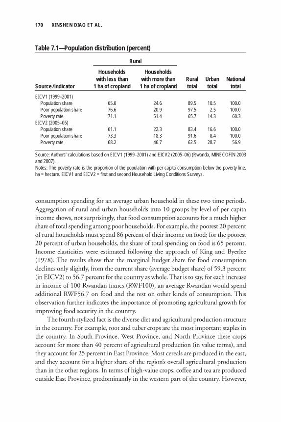
170 XINSHEN DIAO ET AL.
consumption spending for an average urban household in these two time periods. Aggregation of rural and urban households into 10 groups by level of per capita income shows, not surprisingly, that food consumption accounts for a much higher share of total spending among poor households. For example, the poorest 20 percent of rural households must spend 86 percent of their income on food; for the poorest 20 percent of urban households, the share of total spending on food is 65 percent. Income elasticities were estimated following the approach of King and Byerlee (1978). The results show that the marginal budget share for food consumption declines only slightly, from the current share (average budget share) of 59.3 percent (in EICV2) to 56.7 percent for the country as whole. That is to say, for each increase in income of 100 Rwandan francs (RWF100), an average Rwandan would spend additional RWF56.7 on food and the rest on other kinds of consumption. This observation further indicates the importance of promoting agricultural growth for improving food security in the country.
The fourth stylized fact is the diverse diet and agricultural production structure in the country. For example, root and tuber crops are the most important staples in the country. In South Province, West Province, and North Province these crops account for more than 40 percent of agricultural production (in value terms), and they account for 25 percent in East Province. Most cereals are produced in the east, and they account for a higher share of the region’s overall agricultural production than in the other regions. In terms of high-value crops, coffee and tea are produced outside East Province, predominantly in the western part of the country. However,
Table 7.1—Population distribution (percent)
Rural
Households Households with less than with more than Rural Urban NationalSource / indicator 1 ha of cropland 1 ha of cropland total total totalEICV1 (1999–2001) Population share 65.0 24.6 89.5 10.5 100.0 Poor population share 76.6 20.9 97.5 2.5 100.0 Poverty rate 71.1 51.4 65.7 14.3 60.3EICV2 (2005–06) Population share 61.1 22.3 83.4 16.6 100.0 Poor population share 73.3 18.3 91.6 8.4 100.0 Poverty rate 68.2 46.7 62.5 28.7 56.9
Source: Authors’ calculations based on EICV1 (1999–2001) and EICV2 (2005–06) (Rwanda, MINECOFIN 2003 and 2007).Notes: The poverty rate is the proportion of the population with per capita consumption below the poverty line. ha = hectare. EICV1 and EICV2 = first and second Household Living Conditions Surveys.
RWANDA 171
the share of vegetable and fruit production is the highest in the East Province, although the current export opportunities for these crops are small.
The economywide database developed for this study disaggregates the agricul-tural sector to the district level, including the 28 districts that report agricultural production. Production diversifi cation is more obvious at the district level. There are 18 districts that are the most important producers of the country for at least one crop. For example, 38–100 percent of production of export crops (such as tea, coffee, and other cash crops) is concentrated in just three districts. Rice and wheat production is also relatively concentrated, with the three most important districts producing 48.4 percent (rice) and 58.7 percent (wheat) of national production of these crops. The next two most concentrated staples are maize (31.6 percent) and potatoes (33.3 percent). For the remaining crops, the top three producing districts account for less than one-third to one-fi fth of national production. The concentra-tion of production of export and high-value staple crops in a few districts indicates that the gains from promoting growth in such crops are unlikely to be distributed evenly among districts and rural households. Whether such uneven distribution in high-value production affects income distribution and poverty reduction is clearly a policy issue.
Agricultural Policies and Development StrategiesThis section briefl y reviews Rwanda’s recent agricultural strategies. The fi rst com-prehensive strategic document—Vision 2020—was published in 2000 as a result of a broad national consultative process that took place in 1998–99 (Rwanda, MINECOFIN 2000). The major aspiration of Vision 2020 is to transform Rwanda’s economy into a middle-income country with per capita income of US$900 per year by 2020 (from less than US$300). Transformation of agriculture from its current traditional and subsistence system into a productive, high-value, market-oriented sector with forward linkages to other sectors was emphasized in the document. Vision 2020 rightly points out that the most important binding constraint of Rwandan agriculture is its low productivity associated with a traditional subsistence farming system, not the average size of landholdings. Agricultural policy will focus on promoting intensifi cation to increase production. Vision 2020 has provided direction for the country’s agricultural development strategy (in the form of eight key policy areas that need urgent attention to bring about the transformation). However, because it is a rather short document (25 pages), there is no detailed plan in Vision 2020 for any of these policy areas.
In 2002 Rwanda published its fi rst PRSP covering the period up to 2005 (Rwanda, MINECOFIN 2002). In the PRSP, the importance of rural development and agricultural transformation was emphasized and moved to the top of a list of six priority areas (it was the second priority in Vision 2020, after reconstructing the
172 XINSHEN DIAO ET AL.
nation and its social capital on the basis of good governance and a capable state). Moreover, unlike in Vision 2020, agriculture has been integrated into a broad con-cept of rural economic transformation in PRSP 2002. In addition, raising agricul-tural productivity and rural income, including generating opportunities to earn income outside agriculture, have become general goals for this transformation (Rwanda, MINECOFIN 2002, 9).
Agriculture has therefore been chosen as the primary engine of economic growth, and it will be driven by increased fertilizer use (targeted to contribute 75 percent of agricultural growth), along with improvement of wetland management and crop intensifi cation. The PRSP notes that at the current level of technology, smallholder agriculture is the most productive, and the transformation can be achieved by smallholder households who will be supported by energetic public action. The PRSP also emphasizes the increase and diversifi cation of exports, includ-ing agroprocessing exports, to fi nd new engines of growth. The most important development in the PRSP is an explicit discussion on the linkages between agricul-ture and environmental sustainability. The decline in soil fertility in the country “is compounded by soil erosion and the reduction of the water table in some areas and hence agricultural intensifi cation must be accompanied by environmental actions to manage water fl ows, control soil erosion and improve the soil structure” (Rwanda, MINECOFIN 2002, 36).
As a part of the action plans discussed in PRSP 2002, an agricultural sector strategy was developed in 2004 through the National Agricultural Policy (Rwanda, MINAGRI 2004a) and the Strategic Plan for Agricultural Transformation in Rwanda (PSTA) (Rwanda, MINAGRI 2004b). The fi rst part of PSTA provides an overview of typology and characteristics of agricultural farms, sector institutions, rural poverty, food and nutrition, land and labor productivity, and the role of women in agriculture. It also contains an analysis that covers broad aspects of agri-culture, including natural resource management and water and soil conservation; crop and animal production and commodity chains; farmers organizations; agri-business; infrastructure; legal and regulatory framework; and fi nancing, coordina-tion, monitoring, and evaluation of the agricultural sector. The second part of PSTA details the strategic plan, priority programs, expected outputs, and the contribution of other sectors to support agricultural development. The third part of PSTA pro-vides an action plan and estimates fi nancial requirements. Although 10 strategic aspects of agricultural and rural development are highlighted in the second part of PSTA, the document correctly emphasizes that this strategy has to be progressive, fl exible, and dynamic.
PSTA comprises four principal priority programs with 17 subprograms. Their expected results appear in the quantifi ed objectives of the third part of PSTA as the Plan of Action. PSTA also emphasizes the interrelations between the four principal
RWANDA 173
priority programs: (1) intensifi cation and development of sustainable production systems, (2) support to the professionalization of producers, (3) promotion of com-modity chains and development of agribusiness, and (4) institutional development. Each principal priority program further comprises subprograms, and for each sub-program the document provides a brief synthesis of the diagnosis of the current situ-ation, the strategy, specifi c objectives or targets, and specifi c actions. For example, in the fi rst principal priority program (intensifi cation and development of a sustain-able production system), there are fi ve subprograms: (1) sustainable management of natural resources and conservation of water and soils; (2) development of inte-grated agricultural and livestock systems and promotion of specialized intensive animal husbandry; (3) development of marshland and irrigation; (4) supply and use of agricultural inputs; and (5) establishment of food security, implementation of risk management, and evaluation of vulnerability.
The PSTA also includes a table providing indicative and allocated fund esti-mates for each program and subprogram. However, there exists a signifi cant gap between the demands (indicative funds) and supply (allocated funds) in the esti-mates. Although this gap is explicitly presented in the table, the document does not discuss how to fi ll this gap. This raises the question of how to actually prioritize resource allocation to different programs facing a budget constraint that was already clear when the plan was developed, and hence, how to implement these programs when faced with such fi nancial constraints.
There is no doubt that Rwanda’s agricultural strategic plan is a comprehensive document supported by strong evidence developed through a broad consultation process. However, given the constraint of limited fi nancial resources facing the government, how to sequence and prioritize the programs remains a challenge. Moreover, although agriculture is known to be an engine of growth that is generally pro-poor, it still requires empirical evidence to explicitly measure the linkages of growth at the subsector level and overall economic growth and poverty reduction. The analysis in this chapter provides some answers for these highly policy-relevant questions. We fi rst simulate a scenario of modest growth in both agricultural and nonagricultural sectors up to 2015, based on the country’s historical data.
The Rwandan DCGE Model Most existing studies on Rwandan agriculture and agricultural policies are at the microlevel and focus on natural resource management. For example, in a study on farm fragmentation Blarel et al. (1992) used farm-level data for 1987–88 for Rwanda’s three prefectures and found both drawbacks to and possible benefi ts from farm fragmentation for farmers. Clay et al. (1995), in collaboration with the Division of Agricultural Statistics (DSA) of the Rwandan Ministry of Agriculture, measured
174 XINSHEN DIAO ET AL.
both the cost of erosion to land productivity and the returns to soil conversation investments using national farm household survey data between 1983 and 1994. Using data from a similar survey for 1991, Clay (1996) analyzed farmers’ ability and willingness to invest in conservation and soil fertility technologies. The study done by Roose and Ndayizigiye (1997) analyzed water and soil fertility management to fi ght erosion in tropical mountains of Rwanda using plot-level data. A study done by Kelly et al. (2001a), using data from an agricultural survey of 2000’s fi rst season, further emphasized the importance of anti-erosion investment and use of fertilizers to agricultural productivity, rural income, and food security. Beyond agricultural production, Verpoorten and Berlage (2004) conducted a comparison of rural house-hold strategies used to improve income and reduce poverty. The study of von Braun, de Haen, and Blanken (1991) is much more comprehensive; it measures the effects of commercialization in Rwanda on production, income, employment, consump-tion, and nutrition using household survey data.
Although these studies provide detailed knowledge about and policy options for the country’s agricultural and rural economy, a knowledge gap exists in the litera-ture, because no study explicitly focuses on the linkages between the agriculture/rural sector and the rest of economy. Nor do these studies evaluate the contribution of rapid agricultural growth to poverty reduction, and the public investment required to support such growth. The methods used in the previous studies are unsuitable for analyzing these growth linkage issues. We therefore developed a new DCGE model for Rwanda.
A SAM is the underlying database for a DCGE model. The one developed for this analysis is an extended version of the unpublished 2006 SAM of Rwanda con-structed by Arnault (2007). This original SAM was constructed for the national economy and included 51 agricultural and nonagricultural sectors and two primary factors—labor and capital. For the purpose of this study, this SAM has been further disaggregated (see Table 7A.1 in the appendix to this chapter). The key adjustment was to disaggregate agricultural production, households, and primary factors. In our SAM, we fi rst disaggregate all agricultural activities into 30 districts and within each district into two types of farm groups (small farms and medium–large farms) to better capture heterogeneity in production structure across districts. We also dis-aggregate labor into unskilled agricultural labor, unskilled nonagricultural labor, and skilled labor, and we disaggregate capital into capital and agricultural land. We then further disaggregate capital into sector-specifi c capital, economywide agricultural capital, and economywide nonagricultural capital. We assume that land cannot be mobile across districts or among farm groups, which implies that there are 56 cat-egories of land.
In addition to disaggregated primary factors and agricultural production, households and their incomes are further disaggregated. Most Rwandan farmers are
RWANDA 175
involved in staple crop and livestock production, but the opportunities to partici-pate in high-value crop production are not equally distributed among them. For example, tea, one of the country’s most important export crops, is only produced in 10 of the 30 districts, mainly in West Province. Moreover, tea is produced by farmers with large landholdings, though small farmers can participate as laborers. In the case of coffee (the other important export crop of the country), 19 districts produce coffee, but the main production area is concentrated in South Province and West Province. With such uneven distribution in export crop production opportu-nities, if public support concentrates on promoting tea and coffee production and exports, the benefi ts of such a policy would not be likely to reach those farmers outside areas growing tea and coffee. Without a disaggregated SAM, and hence a disaggregated DCGE model, such uneven distribution in the income gains from tea and coffee promotion policies would be ignored, as well as the impact on poverty reduction of such policies.
The disaggregation of the SAM is based on the information drawn from the EICV2 (NISR 2006) and the Rwanda Agricultural Survey 2006 (Rwanda, MINECOFIN 2007). After disaggregation on the production side, there are 960 production activities for 16 crop sectors (16 sectors × 30 districts × 2 types of farms = 960), 270 production activities for 9 livestock sectors (9 sectors × 30 districts = 270), and 28 nonagricultural sectors defi ned at the national level. Sixty-two primary factors are distinguished (3 for labor, 3 for capital, and 56 for land). On the demand side, 62 representative household groups: 60 (30 districts × 2 types of farm households = 60) in the rural area and 2 in the urban area. On the demand side, we also consider the difference between consumption met by farmers’ own production and consump-tion met through the market. The fi rst type of consumption refl ects a subsistence pattern of agricultural production, which exists alongside smallholder agriculture; such consumption is determined by the production that occurred in each district and farm group. Consumption met by the market is more sensitive to change in prices in the market and income received from both agricultural and nonagricultural activities, which are modeled explicitly in the simulations discussed later.
Baseline Growth Scenario Because of sharp production declines in 1994 in Rwanda, the year of the genocide, the post-1994 growth rate was comparatively high and has only recently slowed down. According to World Bank (2008a), during the post-genocide period of 1995–2006, growth rates for total GDP and agricultural GDP (AgGDP) were 7.3 and 6.9 percent annually, respectively, whereas growth has slowed in both total GDP and AgGDP in recent years. During 2002–06 the annual growth rate for total GDP was 4.03 percent, and that for AgGDP was 0.53 percent. This poor
176 XINSHEN DIAO ET AL.
growth performance of AgGDP in the recent period is the refl ection of the severe drought in 2003 after the above-normal harvest of 2002, followed by another bad year in 2004. Even considering a longer period (for example, 2000–06), the annual AgGDP growth is still low (4.1 percent) compared to total GDP growth (5.4 per-cent). Data from Rwanda, MINAGRI (2007) show that total crop production grew at 4.7 percent per year during 2001–07. During this period 30–40 percent of crop production growth was due to area expansion, and the remaining 60–70 percent was due to yield increases (the majority of these increases represented a recovery from the declines of 1994). Clearly, such rapid growth is unsustainable, particularly given the land constraint. Consequently, much more modest land-based expansion is assumed in the model, including the promotion of double cropping and inter-cropping farming practices. Total crop area is assumed to increase by 0.5 percent per year, implying a cumulative increase of about 80,000 ha of cultivated area from 1.69 million ha in 2006 to less than 1.77 million ha by 2015. The growth rates for individual crop yields are chosen to approximate their national average growth rates during 2001–06, with certain adjustments for some crops with particularly high yields during this period (for example, rice grew at 8 percent per year, and vegetables and fruits grew at more than 15 percent).
The base year 2006 was chosen for the model, and the model’s business-as-usual (or baseline) simulation indicates that, with modest growth of 3.8 percent in agri-cultural production together with 5.1 and 5.7 percent annual growth in industry and services, respectively, national GDP grows at 4.8 percent annually, and per capita GDP grows at about 2.9 percent. Crop- or sector-level baseline simulation results are reported in Tables 7.2a and 7.2b (for crop and noncrop sectors, respec-tively). The model result for the growth rate of national GDP is higher than that for 2002–06 (4.0 percent annually) and slightly lower than that for 2001–06 (5.1 percent annually).
The model results also show a modest reduction in national poverty and an improvement in food security. The poverty rate falls to 46.7 percent by 2015, com-pared with 60.3 percent in 2001 (EICV1 data) and 57.0 percent in 2006 (EICV2 data), although the rate was higher in rural areas (63.4 percent) than in urban areas (28.8 percent). Such a reduction in the poverty rate together with population growth results in a decline in the number of the poor of only 220,000 from its cur-rent level of 5.45 million (that is, to 5.23 million by 2015). The poverty reduction in the model as a result of GDP growth is slightly more optimistic than what was experienced in 1999–2005 between the two rounds of household surveys (EICV1 and EICV2). During this period, per capita GDP grew at 2.3 percent annually, while the national poverty rate fell from 60 percent to 57 percent, which indicates that for every percent annual growth in per capita GDP, the national poverty rate fell by 0.42 percent (not percentage point). In the baseline simulation model, 1
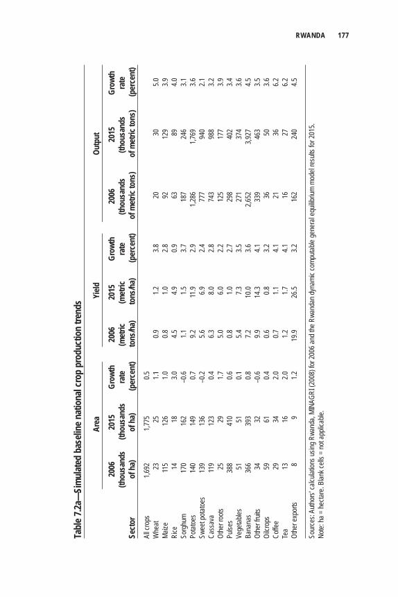
RWANDA 177
Tabl
e 7.2a
—Si
mul
ated
bas
eline
nat
iona
l cro
p pr
oduc
tion
trend
s
Ar
ea
Yield
Ou
tput
20
06
2015
Gr
owth
20
06
2015
Gr
owth
20
06
2015
Gr
owth
(th
ousa
nds
(tho
usan
ds
rate
(m
etric
(m
etric
ra
te
(thou
sand
s (th
ousa
nds
rate
Sect
or
of h
a)
of h
a)
(per
cent
) to
ns/h
a)
tons
/ha)
(p
erce
nt)
of m
etric
tons
) o
f met
ric to
ns)
(per
cent
)Al
l cro
ps
1,692
1,7
75
0.5
W
heat
23
25
1.1
0.9
1.2
3.8
20
30
5.0Ma
ize
115
126
1.0
0.8
1.0
2.8
92
129
3.9Ri
ce
14
18
3.0
4.5
4.9
0.9
63
89
4.0So
rghu
m 17
0 16
2 –0
.6 1.1
1.5
3.7
18
7 24
6 3.1
Potat
oes
140
149
0.7
9.2
11.9
2.9
1,286
1,7
69
3.6Sw
eet p
otatoe
s 13
9 13
6 –0
.2 5.6
6.9
2.4
77
7 94
0 2.1
Cass
ava
119
123
0.4
6.3
8.0
2.8
743
988
3.2Ot
her r
oots
25
29
1.7
5.0
6.0
2.2
125
177
3.9Pu
lses
388
410
0.6
0.8
1.0
2.7
298
402
3.4Ve
getab
les
51
51
0.1
5.4
7.3
3.5
271
374
3.6Ba
nana
s 36
6 39
3 0.8
7.2
10
.0 3.6
2,6
52
3,927
4.5
Othe
r fru
its
34
32
–0.6
9.9
14.3
4.1
339
463
3.5Oi
lcrop
s 59
61
0.4
0.6
0.8
3.2
36
50
3.6
Coffe
e 29
34
2.0
0.7
1.1
4.1
21
36
6.2
Tea
13
16
2.0
1.2
1.7
4.1
16
27
6.2Ot
her e
xpor
ts 8
9 1.2
19
.9 26
.5 3.2
16
2 24
0 4.5
Sour
ces:
Autho
rs’ ca
lculat
ions u
sing R
wand
a, MI
NAGR
I (20
08) f
or 20
06 an
d the
Rwa
ndan
dyna
mic c
ompu
table
gene
ral e
quilib
rium
mode
l resu
lts fo
r 201
5.No
te: ha
= he
ctare
. Blan
k cell
s = no
t app
licab
le.
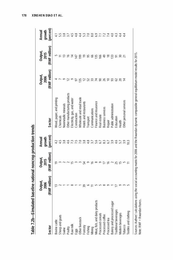
178 XINSHEN DIAO ET AL.
Tabl
e 7.2b
—Si
mul
ated
bas
eline
nat
iona
l non
crop
pro
duct
ion
trend
s
Ou
tput
, Ou
tput
, An
nual
Ou
tput
, Ou
tput
, An
nual
20
06
2015
gr
owth
2006
20
15
grow
thSe
ctor
(R
WF
milli
on)
(RW
F m
illion
) (p
erce
nt)
Sect
or
(RW
F m
illion
) (R
WF
milli
on)
(per
cent
)Bo
vine c
attle
13
19
4.2
Woo
d, pa
per, a
nd pr
inting
4
5 4.1
Shee
p and
goats
2
3 4.5
Ch
emica
ls 7
11
5.5Sw
ine
1 2
3.8
Nonm
etallic
mine
rals
9 13
3.8
Poult
ry 1
2 4.6
Ot
her m
anufa
cturin
g pro
ducts
12
16
3.7
Raw
milk
8 15
7.3
El
ectric
ity, g
as, a
nd w
ater
9 14
4.5
Eggs
1
3 7.5
Co
nstru
ction
97
14
7 4.8
Othe
r live
stock
1
3 7.0
W
holes
ale an
d reta
il tra
de
135
199
4.4Fo
restr
y 39
54
3.8
Ho
tels a
nd re
staur
ants
12
19
5.3Fis
hing
6 9
4.8
Tran
spor
t 52
95
7.0
Minin
g 11
16
3.7
Co
mmun
icatio
ns
33
66
8.0Me
at, fis
h, an
d dair
y pro
ducts
5
8 5.6
Fin
ance
and i
nsur
ance
74
13
5 6.9
Proc
esse
d cer
eals
5 9
6.7
Real
estat
e 90
16
6 7.1
Proc
esse
d coff
ee
8 17
8.3
Bu
sines
s ser
vices
26
49
7.2
Proc
esse
d tea
9
16
6.7
Repa
ir 10
18
7.4
Bake
ry an
d pro
cess
ed su
gar
1 2
3.9
Publi
c adm
inistr
ation
93
13
3 4.0
Trad
itiona
l bev
erag
es
17
25
4.6
Educ
ation
62
91
4.3
Mode
rn be
vera
ges
9 15
5.7
He
alth
20
30
4.4To
bacc
o 3
5 3.9
Ot
her p
erso
nal s
ervic
es
14
21
4.4Te
xtiles
and c
lothin
g 5
11
10.3
Sour
ces:
Autho
rs’ ca
lculat
ions u
sing t
he so
cial a
ccou
nting
matr
ix for
2006
and t
he R
wand
an dy
nami
c com
putab
le ge
nera
l equ
ilibriu
m mo
del re
sults
for 2
015.
Note:
RW
F =
Rwan
dan f
ranc
s.
RWANDA 179
percent of per capita GDP growth results in a 0.71 percent decline in the national poverty rate. The model results also show that the current gap between supply and demand in the food sector would continue to increase. Imports of maize will double, and rice imports will rise by 70 percent by 2015 from their current levels, making Rwanda increasingly dependent on imports or food aid to meet its basic needs for many staple foods.
Accelerated Growth ScenariosQuantitative assessment of how the growth in each agricultural subsector will con-tribute to overall economic growth and poverty reduction is crucial for understand-ing the role of agriculture in broader development. Recent policy debates on agricultural development in Africa have been about such issues as the role of small-holders and that of food staples versus export crops. Despite numerous Asian case studies that have proved the important role of agriculture in development, there is doubt about whether agriculture can successfully generate enough growth in Africa today (see, for example, Collier 2003; Maxwell and Slater 2003; Ellis 2005). With rapid expansion in international agricultural trade, many see high-value commodi-ties, such as fruits, fl owers, and vegetables, as the best opportunities for African farmers. Many African countries are being encouraged to expand into high-value, nontraditional exports and to improve the quality of their traditional tree-crop exports. In Rwanda these sectors, such as coffee and tea, have also attracted more attention and support from the government.
In this section we describe a series of subsector agricultural growth scenarios to specifi cally address these issues. Based on the actual growth targets at the agricultural subsector level, we quantitatively assess the following important policy issues:
1. What is the contribution of each agricultural subsector to broad growth and poverty reduction goals?
2. Why is staple growth so important for overall economic growth and poverty reduction?
3. How can staples-led growth help the country to meet the Comprehensive Africa Agriculture Development Programme (CAADP) goal of 6 percent growth and achieve the fi rst MDG to halve poverty?
4. What is the role of the export agricultural sector?
5. What is the role of nonagricultural growth in this development process?
180 XINSHEN DIAO ET AL.
Although we can simulate growth targets for each crop and subsector, such isolated growth is almost impossible in reality. Thus, we also describe a scenario (the “CAADP scenario”) in which growth occurs simultaneously in all subsectors to meet the targets set by the government. We fi rst discuss the results from this scenario before focusing on individual subsectors.
Agricultural and Total GDP Growth ResultsWith detailed production targets at the agricultural subsector level developed by the Government of Rwanda, such questions as whether these growth targets can support the broad goal of 6 percent agricultural growth and how such growth contributes to halving poverty by 2015 (that is, the fi rst MDG) remain to be answered. The model simulation shows that if the desired targets at the agricultural subsector level can be achieved, then agricultural GDP would grow by 6.3 percent during 2007–15, thus almost doubling the baseline growth rate. This represents total GDP growth of 6 percent, compared with the 4.8 percent baseline level. If additional yearly growth of 2.8 and 2.4 percent is assumed to occur in the industrial and service sectors, respectively, then linkages between nonagriculture and agriculture boost agricultural growth to 6.5 percent per year, while total GDP growth rises to 7.4 percent per year. At this rate, per capita GDP grows at 5.5 percent annually, thus doubling the baseline rate. With such high growth rates, national poverty falls to 35.5 percent by 2015, which is 24.5 percentage points lower than the rate in 1999 and 11.2 percentage points lower than the 2015 baseline. If such growth trends continue until 2020, the country would be able to achieve its fi rst MDG by halving the 1999–2001 poverty rate of 60 percent, albeit only by extending the deadline for achieving that goal to 2020.
Household Income and Poverty EffectsGrowth may not benefi t rural households equally. Empirical studies in other countries often show that rapid economic growth does not always result in shared growth (Akita and Kawamura 2002). Differences in poverty reduction and income growth across regions have also been observed in China (Chen and Raval-lion 2000; Kanbur and Zhang 2004). Thus, it is essential to further assess the income and poverty effects of agricultural growth at the household level.
In the case of Rwanda, the simulation results indicate that rapid agricul-tural growth benefi ts the majority of rural households and that the distribu-tion of benefi ts is relatively equal. Nevertheless, the household group with the small landholdings appears to benefi t less than the household group with medium–large landholdings. In the scenario in which both agriculture and nonagriculture grow, annual income growth for the small-farm group at the national level is 8.5 percent, whereas it is 9.0 percent for the household group with larger land-holdings (Table 7.3). Rural poverty falls across provinces and household groups,
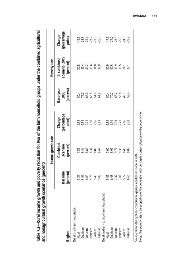
RWANDA 181
Tabl
e 7.3—
Rura
l inco
me g
rowt
h an
d po
verty
redu
ctio
n fo
r two
of t
he fa
rm h
ouse
hold
gro
ups u
nder
the c
ombi
ned
agric
ultu
ral
and
nona
gricu
ltura
l gro
wth
scen
ario
s (pe
rcen
t)
In
com
e gro
wth
rate
Po
verty
rate
Com
bine
d Ch
ange
Ba
se-y
ear,
In
com
bine
d Ch
ange
Ba
selin
e sc
enar
io
(per
cent
age
2006
sc
enar
io, 2
015
(per
cent
age
Regi
on
(per
cent
) (p
erce
nt)
poi
nt)
(per
cent
) (p
erce
nt)
poin
t)Ru
ral s
mall-f
arm
hous
ehold
s
Kiga
li 5.2
7 7.8
6 2.5
9 50
.4 30
.8 –1
9.6
South
ern
5.91
8.44
2.53
72.7
47.4
–25.3
W
ester
n 6.0
9 8.8
2 2.7
3 65
.6 40
.2 –2
5.4
North
ern
5.78
8.37
2.58
66.8
39.6
–27.2
Ea
stern
5.4
3 8.0
9 2.6
5 54
.0 31
.0 –2
3.0
Natio
nal
5.83
8.47
2.63
64.9
39.9
–25.0
Rura
l med
ium- t
o lar
ge-fa
rm ho
useh
olds
Kiga
li 5.0
5 7.6
0 2.5
6 50
.4 32
.9 –1
7.5
South
ern
6.98
8.97
1.99
70.2
42.5
–27.7
W
ester
n 7.4
7 9.7
7 2.3
1 63
.2 39
.9 –2
3.3
North
ern
7.06
9.35
2.29
58.8
33.5
–25.3
Ea
stern
5.7
7 8.4
3 2.6
6 48
.7 24
.1 –2
4.6
Natio
nal
6.65
9.03
2.38
58.4
33.1
–25.2
Sour
ce: R
wand
an dy
nami
c com
putab
le ge
nera
l equ
ilibriu
m mo
del re
sults
.No
te: T
he po
verty
rate
is the
prop
ortio
n of th
e pop
ulatio
n with
per c
apita
cons
umpti
on be
low th
e pov
erty
line.
182 XINSHEN DIAO ET AL.
but at the national level poverty falls more among the group with larger land-holdings than among the small-farm group. As the initial poverty rate is already higher among small farmers, the difference in the poverty rate between these two types of rural households is further widened by 2015. At the provincial level, the poverty rate is highest in the South Province for both household groups. Although the initial poverty rate of the southern small-farm group is 2.5 per-centage points higher than that of the southern large-farm group, the poverty gap between these two groups increases to 4.9 percentage points by 2015.
Subsector Growth and Poverty-Reduction ImpactsThe different poverty-reduction effects of growth at the province level and among different types of farm households relate to the different income sources of farmers and the local agricultural production structure they face. Thus, as differing growth–poverty linkages can occur in the agricultural subsector, it is important to under-stand such linkages when designing pro-poor growth strategies. For this purpose, the poverty–growth elasticity was calculated to enable direct comparison of the vari-ous poverty-reduction outcomes. This elasticity was calculated for the two broad agricultural products—staple food and export crops—as well as for each individual crop or livestock product for which targeted growth was individually simulated.
Although agricultural growth is generally pro-poor, a gap in the poverty–growth elasticities between staple crops, such as grains and roots, and agricultural exports indicates the importance of staples for poorer rural households. If economy-wide growth is led by growth in grain crops, each 1 percent additional growth in per capita GDP leads to an additional 1.74 percent decline in the national poverty rate. The growth–poverty-reduction effect is particularly large in the case of maize, which has an elasticity of –2.39 (Table 7.4). In contrast, if economywide growth is led by growth in export crops, including both traditional export crops (such as coffee and tea) and nontraditional ones (such as vegetables and fruits), a 1 percent addi-tional growth in per capita GDP reduces the national poverty rate by 1.68 percent.
The model results indicate that putting staples at the top of the agenda can promote broader economic progress and poverty reduction in Rwanda. This is true in general in many African countries, as smallholders comprise more than 70 per-cent of the continent’s farmers (Johnson, Hazell, and Gulati 2003). A wide range of research has also demonstrated the importance of food staples in driving growth and contributing to a dynamic structural transformation of rural economies (Byerlee, Diao, and Jackson 2005; Bezemer and Headey 2008; World Bank, 2008b; Diao, Hazell, and Thurlow 2010). Acceleration in staples production has also been found to produce secondary and tertiary effects on the broader economy by reducing food prices for urban consumers, curbing overall infl ation, and releasing scarce foreign exchange for the importation of goods that are typically unsuited to production in
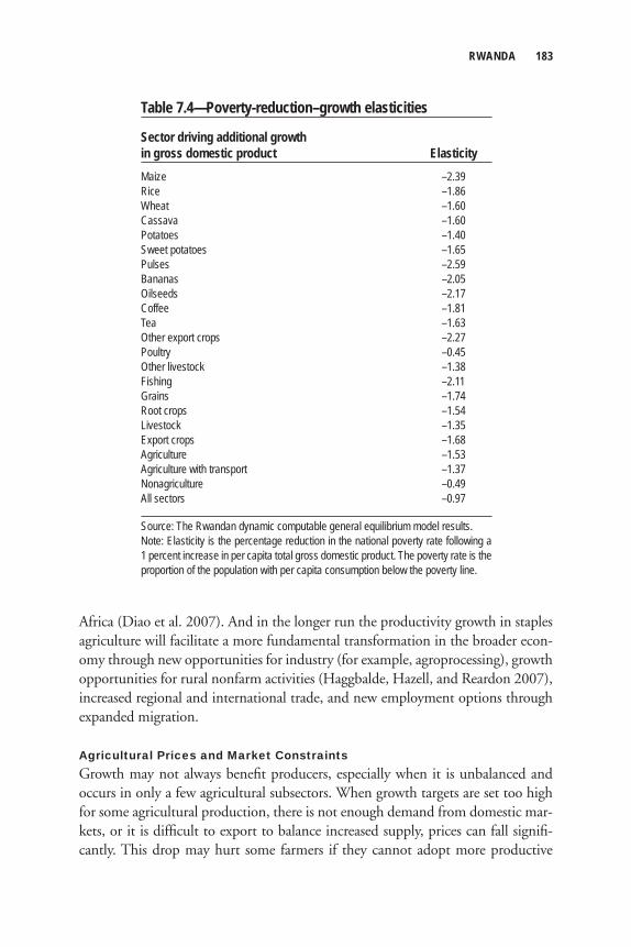
RWANDA 183
Africa (Diao et al. 2007). And in the longer run the productivity growth in staples agriculture will facilitate a more fundamental transformation in the broader econ-omy through new opportunities for industry (for example, agroprocessing), growth opportunities for rural nonfarm activities (Haggbalde, Hazell, and Reardon 2007), increased regional and international trade, and new employment options through expanded migration.
Agricultural Prices and Market Constraints Growth may not always benefi t producers, especially when it is unbalanced and occurs in only a few agricultural subsectors. When growth targets are set too high for some agricultural production, there is not enough demand from domestic mar-kets, or it is diffi cult to export to balance increased supply, prices can fall signifi -cantly. This drop may hurt some farmers if they cannot adopt more productive
Table 7.4—Poverty-reduction–growth elasticities
Sector driving additional growth in gross domestic product ElasticityMaize –2.39Rice –1.86Wheat –1.60Cassava –1.60Potatoes –1.40Sweet potatoes –1.65Pulses –2.59Bananas –2.05Oilseeds –2.17Coffee –1.81Tea –1.63Other export crops –2.27Poultry –0.45Other livestock –1.38Fishing –2.11Grains –1.74Root crops –1.54Livestock –1.35Export crops –1.68Agriculture –1.53Agriculture with transport –1.37Nonagriculture –0.49All sectors –0.97
Source: The Rwandan dynamic computable general equilibrium model results.Note: Elasticity is the percentage reduction in the national poverty rate following a 1 percent increase in per capita total gross domestic product. The poverty rate is the proportion of the population with per capita consumption below the poverty line.
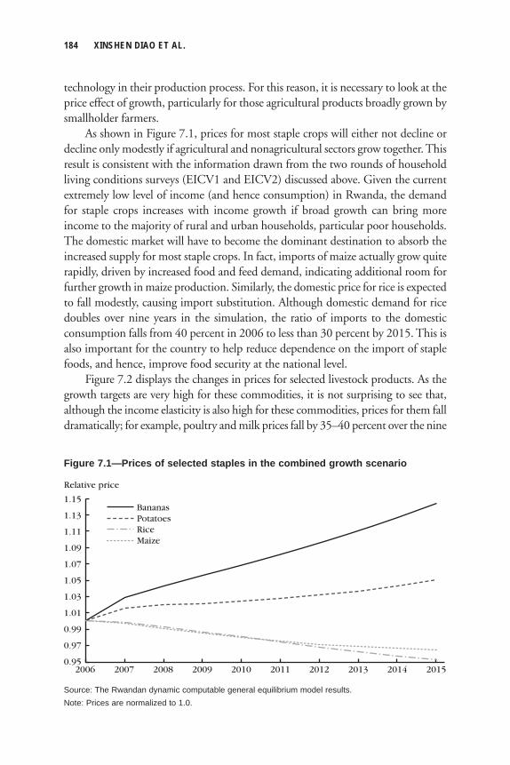
184 XINSHEN DIAO ET AL.
technology in their production process. For this reason, it is necessary to look at the price effect of growth, particularly for those agricultural products broadly grown by smallholder farmers.
As shown in Figure 7.1, prices for most staple crops will either not decline or decline only modestly if agricultural and nonagricultural sectors grow together. This result is consistent with the information drawn from the two rounds of household living conditions surveys (EICV1 and EICV2) discussed above. Given the current extremely low level of income (and hence consumption) in Rwanda, the demand for staple crops increases with income growth if broad growth can bring more income to the majority of rural and urban households, particular poor households. The domestic market will have to become the dominant destination to absorb the increased supply for most staple crops. In fact, imports of maize actually grow quite rapidly, driven by increased food and feed demand, indicating additional room for further growth in maize production. Similarly, the domestic price for rice is expected to fall modestly, causing import substitution. Although domestic demand for rice doubles over nine years in the simulation, the ratio of imports to the domestic consumption falls from 40 percent in 2006 to less than 30 percent by 2015. This is also important for the country to help reduce dependence on the import of staple foods, and hence, improve food security at the national level.
Figure 7.2 displays the changes in prices for selected livestock products. As the growth targets are very high for these commodities, it is not surprising to see that, although the income elasticity is also high for these commodities, prices for them fall dramatically; for example, poultry and milk prices fall by 35–40 percent over the nine
2015201420132012201120102009200820072006
Relative price
1.15
0.95
1.09
1.05
0.99
1.01
1.03
1.07
1.11
1.13
0.97
BananasPotatoesRiceMaize
Figure 7.1—Prices of selected staples in the combined growth scenario
Source: The Rwandan dynamic computable general equilibrium model results.Note: Prices are normalized to 1.0.
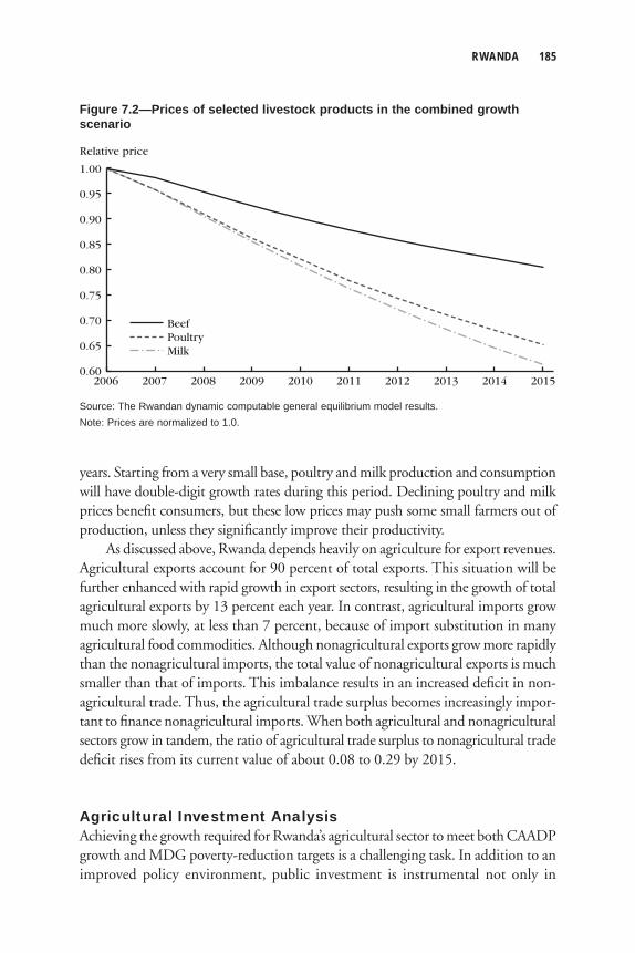
RWANDA 185
years. Starting from a very small base, poultry and milk production and consumption will have double-digit growth rates during this period. Declining poultry and milk prices benefi t consumers, but these low prices may push some small farmers out of production, unless they signifi cantly improve their productivity.
As discussed above, Rwanda depends heavily on agriculture for export revenues. Agricultural exports account for 90 percent of total exports. This situation will be further enhanced with rapid growth in export sectors, resulting in the growth of total agricultural exports by 13 percent each year. In contrast, agricultural imports grow much more slowly, at less than 7 percent, because of import substitution in many agricultural food commodities. Although nonagricultural exports grow more rapidly than the nonagricultural imports, the total value of nonagricultural exports is much smaller than that of imports. This imbalance results in an increased defi cit in non-agricultural trade. Thus, the agricultural trade surplus becomes increasingly impor-tant to fi nance nonagricultural imports. When both agricultural and nonagricultural sectors grow in tandem, the ratio of agricultural trade surplus to nonagricultural trade defi cit rises from its current value of about 0.08 to 0.29 by 2015.
Agricultural Investment AnalysisAchieving the growth required for Rwanda’s agricultural sector to meet both CAADP growth and MDG poverty-reduction targets is a challenging task. In addition to an improved policy environment, public investment is instrumental not only in
Relative price
1.00
0.60
0.90
0.80
0.70
0.65
0.75
0.85
0.95
2015201420132012201120102009200820072006
BeefPoultryMilk
Figure 7.2—Prices of selected livestock products in the combined growth scenario
Source: The Rwandan dynamic computable general equilibrium model results.Note: Prices are normalized to 1.0.
186 XINSHEN DIAO ET AL.
improving public services and provision (such as research and extension, rural infra-structure, and education) but also in attracting private investment and inputs. The following discussion focuses on public sector spending on agriculture required to achieve these goals and the potential returns to investments in different subsectors of agriculture.
The previous analysis indicates that agricultural GDP could grow at more than 6 percent annually over nine years in the simulation if agricultural commodity or subsector growth can reach national targets identifi ed by the Government of Rwanda. These growth targets are consistent with CAADP goals and will signifi -cantly reduce poverty. The model results show that with more than 6 percent growth in agriculture together with rapid growth in the nonagricultural sector, Rwanda will be able to achieve the fi rst MDG of halving poverty by 2020.
To promote more rapid agricultural growth and greater poverty reduction, the Government of Rwanda has already committed to increasing its investment in agriculture, and many agricultural development programs are being implemented. Moreover, the government has also increased investment in rural infrastructure, markets, and supply chains to improve the external environment for agricultural growth and rural development. Such large-scale public investment is not only neces-sary for agricultural growth and rural development but is also a precondition for the private sector, including farmers, to increase their investments. All these interven-tions and investments will build a solid foundation for enhanced agricultural growth, but the short implementation period makes ex post assessment of the impacts of these endeavors on future growth diffi cult. For this reason, an ex ante approach is developed for this chapter. We fi rst focus on the amount of public investment in agriculture required for achieving the growth targets discussed in the previous section. We then introduce the newly developed ex ante approach and apply it to assess the potential returns of agricultural investment and the relationship between targeted growth and increased agricultural investment at the subsector level.
Estimating Total Spending Required for Agricultural Growth Offi cial national agricultural spending data are only available for 2001–06; addi-tional data (1995–2000) were drawn from IMF (2004). The estimated elasticity of agricultural growth with respect to agricultural spending during 1995–2005 is 0.17. This elasticity is much lower than the African average of 0.366, which is based on cross-country estimations using a much longer data time series (Fan, Yu, and Saurkar 2008). Because of Rwanda’s recent history and the large amount of spend-ing required to recover basic agricultural production in genocide-affected areas, the estimated elasticity for agricultural spending–agricultural growth may not represent the true relationship in the future. Moreover, many productive investment projects
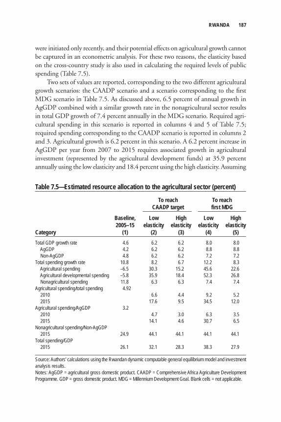
RWANDA 187
were initiated only recently, and their potential effects on agricultural growth cannot be captured in an econometric analysis. For these two reasons, the elasticity based on the cross-country study is also used in calculating the required levels of public spending (Table 7.5).
Two sets of values are reported, corresponding to the two different agricultural growth scenarios: the CAADP scenario and a scenario corresponding to the fi rst MDG scenario in Table 7.5. As discussed above, 6.5 percent of annual growth in AgGDP combined with a similar growth rate in the nonagricultural sector results in total GDP growth of 7.4 percent annually in the MDG scenario. Required agri-cultural spending in this scenario is reported in columns 4 and 5 of Table 7.5; required spending corresponding to the CAADP scenario is reported in columns 2 and 3. Agricultural growth is 6.2 percent in this scenario. A 6.2 percent increase in AgGDP per year from 2007 to 2015 requires associated growth in agricultural investment (represented by the agricultural development funds) at 35.9 percent annually using the low elasticity and 18.4 percent using the high elasticity. Assuming
Table 7.5—Estimated resource allocation to the agricultural sector (percent)
To reach To reach CAADP target first MDG
Baseline, Low High Low High 2005–15 elasticity elasticity elasticity elasticityCategory (1) (2) (3) (4) (5)Total GDP growth rate 4.6 6.2 6.2 8.0 8.0 AgGDP 4.2 6.2 6.2 8.8 8.8 Non-AgGDP 4.8 6.2 6.2 7.2 7.2Total spending growth rate 10.8 8.2 6.7 12.2 8.3 Agricultural spending –6.5 30.3 15.2 45.6 22.6 Agricultural developmental spending –5.8 35.9 18.4 52.3 26.8 Nonagricultural spending 11.8 6.3 6.3 7.4 7.4Agricultural spending/total spending 4.92 2010 6.6 4.4 9.2 5.2 2015 17.6 9.5 34.5 12.0Agricultural spending/AgGDP 3.2 2010 4.7 3.0 6.3 3.5 2015 14.1 4.6 30.7 6.5Nonagricultural spending/Non-AgGDP 2015 24.9 44.1 44.1 44.1 44.1Total spending/GDP 2015 26.1 32.1 28.3 38.3 27.9
Source: Authors’ calculations using the Rwandan dynamic computable general equilibrium model and investment analysis results.Notes: AgGDP = agricultural gross domestic product. CAADP = Comprehensive Africa Agriculture Development Programme. GDP = gross domestic product. MDG = Millennium Development Goal. Blank cells = not applicable.
188 XINSHEN DIAO ET AL.
that the government’s allocation to nonagricultural sectors is proportional to non-agricultural GDP and that nondevelopmental spending on agriculture is propor-tional to AgGDP, the total government budget is estimated to grow at 6.7 percent using the high elasticity and at 8.2 percent using the low elasticity.
The spending growth estimate is consistent with the average growth in the total government budget observed in recent years, but the agricultural spending requires much faster growth than in the past. Because of more rapid growth in agricultural spending than in the total spending growth, the agricultural spending share will rise to 4.4 or 6.6 percent in 2010 and 9.5 or 17.6 percent in 2015, where the lower number is for the high elasticity and the higher one is for the low elasticity (Table 7.5, columns 2 and 3). Whether the government needs to meet requirements of the Maputo Declaration of allocating at least 10 percent of its total budget to agriculture depends on whether agricultural spending can stimulate agricultural growth effi -ciently. With lower effi ciency (that is, low elasticity pertains), the government needs to allocate 18 percent of its total budget to agriculture by 2015, but if spending is more effi cient (that is, high elasticity is appropriate), about 10 percent of the total government budget would be needed to support 6 percent annual agricultural growth.
Six percent annual agricultural growth for nine years is insuffi cient for the country to meet the goal of halving national poverty by 2020. Instead, a growth rate of 6.5 percent per year during 2007–20 is needed. Estimates of the required spend-ing to achieve this level of growth are provided in Table 7.5 (columns 4 and 5), indicating that agricultural spending needs to grow at the extremely high rate of 45.6 percent annually (2007–15) if investment has a low elasticity, or 22.6 percent if the investment is more effi cient. Assuming that growth in nonagricultural spend-ing is proportional to nonagricultural GDP and that nondevelopmental spending on agriculture is proportional to AgGDP, then the total government budget would grow at 8.3 or 12.2 percent annually, depending on whether the elasticity was high or low, respectively. The share of agricultural spending would rise to 5.2–9.2 percent in 2010 and 12.0–34.5 percent in 2015, again based on which elasticity is realized.
Although the required rate of growth in public resources allocated to the agri-cultural sector seems unrealistically high, the resulting shares of agricultural spend-ing are not uncommonly high based on the experiences of many Asian countries in their early stages of development. The analysis here indicates one of the important challenges facing the Rwandan government in prioritizing public fund allocation, as it has shown an inconsistency between the current budget allocation and the role of agriculture as the engine of overall growth and the most important contributor to poverty reduction proposed in government strategic documents (Rwanda, MINECOFIN, 2000, 2002, 2008). On a positive note, the government has already
RWANDA 189
recognized such inconsistency and has started to increase the allocation to the agri-cultural sector and rural development in the second EDPRS for 2008–12. However, there is still a signifi cant gap between required increases and planned increases in agricultural spending. This analysis also raises an important issue of improving the effi ciency of public spending. When the spending effi ciency can be improved to a level representative of the African average, growth in required agricultural spending as well as share of agricultural spending in total budget can be cut by more than half. Increasing the effi ciency of public investment requires more studies on institutional and governance capacity and policy implementation process, which is important but goes beyond the scope of this chapter.
Assessing Investment Priorities by Estimating Potential Returns to Investment Estimating the public resources needed to reach the overall agricultural growth target is important, but prioritizing investments is equally important. To prioritize the allocation of public investment, it is necessary to measure the returns to invest-ment. Public investment will generate externalities and directly and indirectly affect broad economic performance. Hence, it may underestimate the impact of public agricultural investment if the gains are narrowly measured for individual sectors that directly benefi t from the interventions. Moreover, as we have shown in the previous section, agriculture-led growth is pro-poor, and the relationship between public investment in agriculture and poverty reduction needs to be taken into account when the impact of agricultural investment is assessed. In this section we combine the public investment analysis with the DCGE model to assess the potential returns to agricultural investment from an economywide perspective.
As previously mentioned, constrained by the short period of existing invest-ment data in Rwanda stemming from historical reasons, it is not possible to conduct an ex post econometric analysis for evaluating the returns to public investment in agriculture. A different approach has to be applied so that the available data can be used to the greatest extent possible. With help from MINAGRI we have obtained a spending plan with detailed target and costing information, prepared for the second EDPRS. Based on the information received and other data drawn from the literature, we have developed an ex ante approach to organize this information as inputs into the DCGE model. We then use the DCGE model to conduct a series of simulation analyses to assess the returns to public investment in the agricultural sector.
Table 7.6 summarizes the total amount of public investment in agriculture planned for 2007–15, drawn from Rwanda, MINECOFIN (2008). The original assessment of national needs to achieve the EPDRS targets is for a fi ve-year period (2008–12). To be consistent with the fi rst MDG time frame, we decided to consider
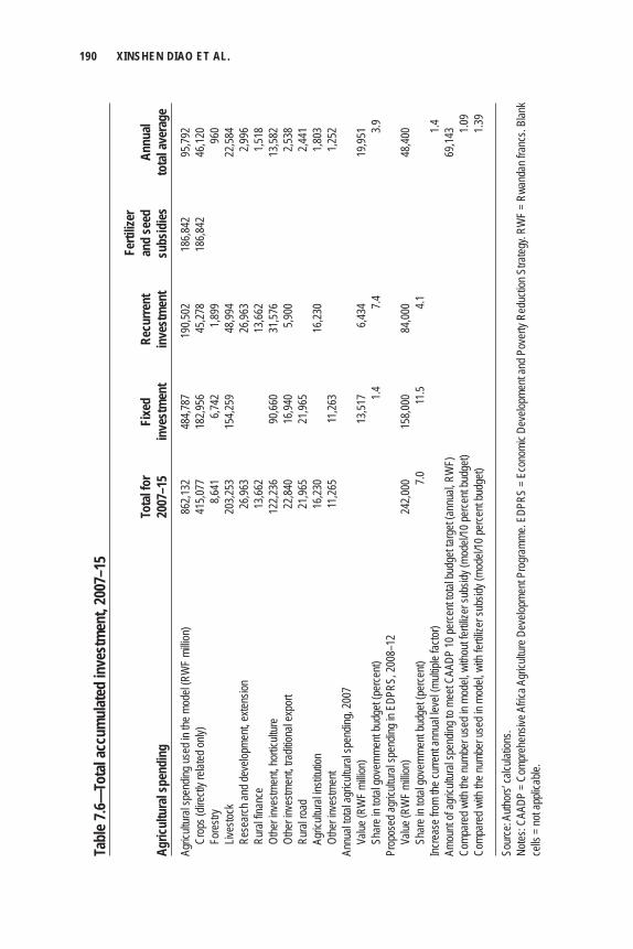
190 XINSHEN DIAO ET AL.
Tabl
e 7.6—
Tota
l acc
umul
ated
inve
stm
ent,
2007
–15
Ferti
lizer
To
tal f
or
Fixe
d Re
curre
nt
and
seed
An
nual
Agric
ultu
ral s
pend
ing
2007
–15
inve
stm
ent
inve
stm
ent
subs
idies
to
tal a
vera
geAg
ricult
ural
spen
ding u
sed i
n the
mod
el (R
WF
millio
n)
862,1
32
484,7
87
190,5
02
186,8
42
95,79
2
Crop
s (dir
ectly
relat
ed on
ly)
415,0
77
182,9
56
45,27
8 18
6,842
46
,120
Fo
restr
y 8,6
41
6,742
1,8
99
96
0
Lives
tock
203,2
53
154,2
59
48,99
4
22,58
4
Rese
arch
and d
evelo
pmen
t, exte
nsion
26
,963
26
,963
2,9
96
Rura
l fina
nce
13,66
2
13,66
2
1,518
Ot
her in
vestm
ent, h
ortic
ultur
e 12
2,236
90
,660
31,57
6
13,58
2
Othe
r inve
stmen
t, tra
dition
al ex
port
22,84
0 16
,940
5,900
2,538
Ru
ral ro
ad
21,96
5 21
,965
2,441
Ag
ricult
ural
institu
tion
16,23
0
16,23
0
1,803
Ot
her in
vestm
ent
11,26
5 11
,263
1,252
Annu
al tot
al ag
ricult
ural
spen
ding,
2007
Va
lue (R
WF
millio
n)
13
,517
6,434
19,95
1
Shar
e in t
otal g
over
nmen
t bud
get (
perce
nt)
1.4
7.4
3.9Pr
opos
ed ag
ricult
ural
spen
ding i
n EDP
RS, 2
008–
12
Value
(RW
F mi
llion)
24
2,000
15
8,000
84
,000
48
,400
Sh
are i
n tota
l gov
ernm
ent b
udge
t (pe
rcent)
7.0
11
.5 4.1
Incre
ase f
rom
the cu
rrent
annu
al lev
el (m
ultipl
e fac
tor)
1.4Am
ount
of ag
ricult
ural
spen
ding t
o mee
t CAA
DP 10
perce
nt tot
al bu
dget
targe
t (an
nual,
RW
F)
69
,143
Comp
ared
with
the n
umbe
r use
d in m
odel,
with
out fe
rtilize
r sub
sidy (
mode
l/10 p
erce
nt bu
dget)
1.09
Comp
ared
with
the n
umbe
r use
d in m
odel,
with
fertil
izer s
ubsid
y (mo
del/1
0 per
cent
budg
et)
1.3
9
Sour
ce: A
uthor
s’ ca
lculat
ions.
Notes
: CAA
DP =
Com
preh
ensiv
e Afric
a Agr
icultu
re D
evelo
pmen
t Pro
gram
me. E
DPRS
= E
cono
mic D
evelo
pmen
t and
Pov
erty
Redu
ction
Stra
tegy.
RWF
= Rw
anda
n fra
ncs.
Blan
k ce
lls =
not a
pplic
able.
RWANDA 191
a nine-year period (2007–15) for the analysis. Moreover, the initial assessment of the public investment required by the EDPRS targets had to be scaled down because of budget constraints set by the Rwandan Ministry of Finance. The fi nal agreed-on total spending for agriculture is about 30 percent of what had been originally planned (see second part of Table 7.6). However, for this analysis we decided to use the original budget allocation for the following three reasons. First, the purpose of this analysis is to provide an assessment of actual requirements in agricultural invest-ment for achieving both the CAADP growth target and the fi rst MDG goal of halving poverty by 2020. After assessing the growth requirement in the previous chapter of the report, it is necessary to understand the cost of such growth with a complete picture without taking into account the budget constraints. Second, our analysis considers the nine years between 2007 and 2015. Without scaling down the total cost planned by MINAGRI, we can slightly reduce the annual cost by allocating the same amount of total spending over the nine years instead of over fi ve years (annual spending is still about 50 percent higher in our analysis than that included in the EDPRS; see the annual average column of Table 7.6 for compari-son). Third, we also consider the CAADP targets, one of which requires African countries to allocate at least 10 percent of government spending to agriculture. The amount of agricultural spending, if it is based on the originally planned numbers of MINAGRI, will allow the agricultural sector to reach 10 percent of total govern-ment budget.1
The key information about budget allocation and targets to be achieved through such public investment (such as how many hectares of irrigated land or how many metric tons of improved seeds will be developed) is available in the dataset received from MINAGRI. Subsidies for fertilizer and improved seeds are not considered in the government budget allocation but are added as a part of public spending in the above budget allocation. As in many other African countries, the past poor perfor-mance of the agricultural sector in Rwanda is partly a consequence of the very limited use of improved seeds and fertilizers. According to Kelly et al. (2001b), average consumption of fertilizer per hectare of cultivated land is less than 4 kilo-grams (kg) in Rwanda. This value contrasts sharply with Sub-Saharan Africa as a whole (ranging from 9 to 11 kg/ha). The average level of use of improved seed is also low, only about 1.3 percent of total seed applied, a level also below the average for Sub-Saharan Africa (Fowler et al. 2007). With increased world oil prices, fertil-izer prices have become unaffordable for the majority of small farmers in Africa. Thus, a partial subsidy on imports of fertilizer is seen as a necessary step to increase the use of fertilizer in crop production.
The above budget allocation information is important for any analysis to assess the economic outcome of public investment allocation; however, such information alone is not enough. To assess the impact of public investment on the growth and
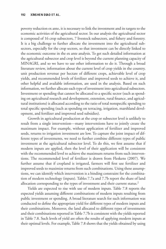
192 XINSHEN DIAO ET AL.
poverty reduction ex ante, it is necessary to link the investment and its targets to the economic activities of the agricultural sector. In our analysis the agricultural sector is composed of 16 crop subsectors, 7 livestock subsectors, and fi shery and forestry. It is a big challenge to further allocate the investment into the agricultural sub-sectors, especially for the crop sectors, so that investment can be directly linked to the economic outcome in the ex ante analysis. To get such detailed information at the agricultural subsector and crop level is beyond the current planning capacity of MINAGRI, and so we have to use other information to do it. Through a broad literature review, information about the current level of crop yields in the country, unit production revenue per hectare of different crops, achievable level of crop yields, and recommended levels of fertilizer and improved seeds to achieve it, and other helpful and available information, are used in the analysis. Based on such information, we further allocate each type of investment into agricultural subsectors. Investment or spending that cannot be allocated to a specifi c sector (such as spend-ing on agricultural research and development, extension, rural fi nance, and agricul-tural institutions) is allocated according to the ratio of total nonspecifi c spending to total specifi c spending (such as spending on terracing, irrigation, marshland devel-opment, and fertilizer and improved seed subsidies).
Growth in agricultural production at the crop or subsector level is unlikely to result from a single intervention—many interventions have to jointly create the maximum impact. For example, without application of fertilizer and improved seeds, returns to irrigation investment are low. To capture the joint impact of dif-ferent types of investments, we need to further combine different types of public investment at the agricultural subsector level. To do this, we fi rst assume that if modern inputs are applied, then the level of their application will be consistent with the recommended level to achieve the maximum returns from such interven-tions. The recommended level of fertilizer is drawn from Fleskens (2007). We further assume that if cropland is irrigated, farmers will fi rst use fertilizer and improved seeds to maximize returns from such combinations. Using these assump-tions, we can identify which intervention is a binding constraint for the combina-tion of modern technology (inputs). Tables 7.7a and 7.7b report the share of land allocation corresponding to the types of investment and their current status.2
Yields are expected to rise with use of modern inputs. Table 7.8 reports the expected yields assuming different combinations of modern inputs resulting from public investment or spending. A broad literature search for such information was conducted to defi ne the appropriate yield for different types of modern inputs and their combinations. Moreover, the land allocated to different types of investments and their combinations reported in Table 7.7b is consistent with the yields reported in Table 7.8. Such levels of yield are often the results of applying modern inputs at their optimal levels. For example, Table 7.8 shows that the yields obtained by using
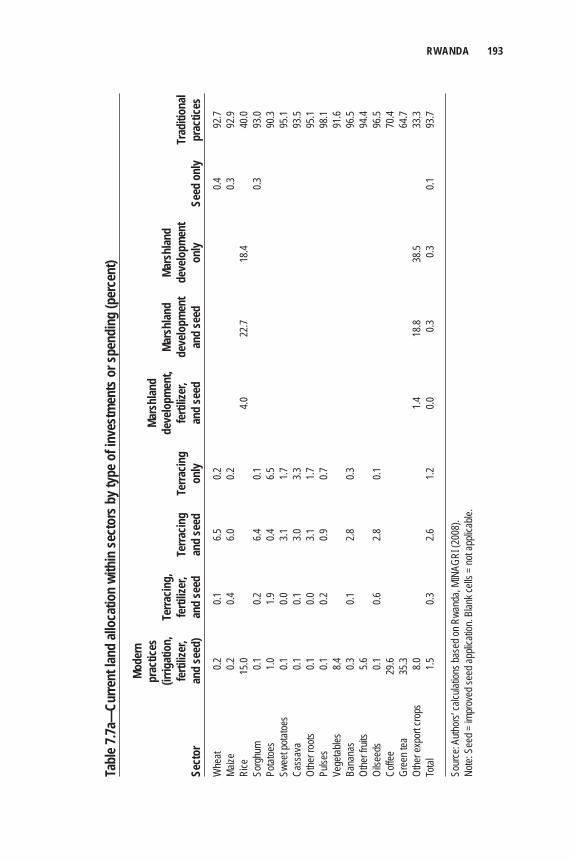
RWANDA 193
Tabl
e 7.7a
—Cu
rrent
land
allo
catio
n wi
thin
sect
ors b
y typ
e of i
nves
tmen
ts o
r spe
ndin
g (p
erce
nt)
Mo
dern
pr
actic
es
Ma
rshl
and
(ir
rigat
ion,
Te
rracin
g,
deve
lopm
ent,
Mars
hlan
d Ma
rshl
and
fe
rtiliz
er,
ferti
lizer
, Te
rracin
g Te
rracin
g fe
rtiliz
er,
deve
lopm
ent
deve
lopm
ent
Tr
aditi
onal
Sect
or
and
seed
) an
d se
ed
and
seed
on
ly an
d se
ed
and
seed
on
ly Se
ed o
nly
prac
tices
Whe
at 0.2
0.1
6.5
0.2
0.4
92.7
Maize
0.2
0.4
6.0
0.2
0.3
92.9
Rice
15
.0
4.0
22.7
18.4
40
.0So
rghu
m 0.1
0.2
6.4
0.1
0.3
93.0
Potat
oes
1.0
1.9
0.4
6.5
90.3
Swee
t pota
toes
0.1
0.0
3.1
1.7
95.1
Cass
ava
0.1
0.1
3.0
3.3
93.5
Othe
r roo
ts 0.1
0.0
3.1
1.7
95
.1Pu
lses
0.1
0.2
0.9
0.7
98.1
Vege
tables
8.4
91.6
Bana
nas
0.3
0.1
2.8
0.3
96.5
Othe
r fru
its
5.6
94
.4Oi
lseed
s 0.1
0.6
2.8
0.1
96
.5Co
ffee
29.6
70
.4Gr
een t
ea
35.3
64
.7Ot
her e
xpor
t cro
ps
8.0
1.4
18
.8 38
.5
33.3
Total
1.5
0.3
2.6
1.2
0.0
0.3
0.3
0.1
93
.7
Sour
ce: A
uthor
s’ ca
lculat
ions b
ased
on R
wand
a, MI
NAGR
I (20
08).
Note:
See
d = im
prov
ed se
ed ap
plica
tion.
Blan
k cell
s = no
t app
licab
le.
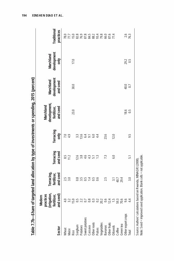
194 XINSHEN DIAO ET AL.
Tabl
e 7.7b
—Sh
are o
f tar
gete
d lan
d all
ocat
ion
by ty
pe o
f inv
estm
ents
or s
pend
ing,
2015
(per
cent
)
Mo
dern
pr
actic
es
Ma
rshl
and
(ir
rigat
ion,
Te
rracin
g,
deve
lopm
ent,
Mars
hlan
d Ma
rshl
and
fe
rtiliz
er,
ferti
lizer
, Te
rracin
g Te
rracin
g fe
rtiliz
er,
deve
lopm
ent
deve
lopm
ent
Trad
ition
alSe
ctor
an
d se
ed)
and
seed
an
d se
ed
only
and
seed
an
d se
ed
only
prac
tices
Whe
at 4.0
2.5
8.5
7.0
78.0
Maize
3.2
3.0
11
.2 4.9
77.7
Rice
15
.0
23.0
30.0
17.0
15.0
Sorg
hum
0.5
0.8
12.6
3.3
82
.8Po
tatoe
s 2.2
3.5
3.8
13
.6
76.9
Swee
t pota
toes
0.7
0.5
4.6
6.4
87
.8Ca
ssav
a 0.8
1.4
4.3
9.1
84.5
Othe
r roo
ts 0.3
0.5
5.1
6.0
88.2
Pulse
s 0.2
0.6
1.3
4.4
93.4
Vege
tables
20
.2
79
.8Ba
nana
s 0.6
2.5
7.3
23
.6
66.0
Othe
r fru
its
12.4
87.6
Oilse
eds
1.5
3.1
6.0
12.0
77
.4Co
ffee
59.3
40.7
Gr
een t
ea
70.6
29.4
Ot
her e
xpor
t cro
ps
9.6
18
.6 40
.0 29
.2 2.6
Total
4.4
3.0
5.1
9.5
0.5
0.7
0.5
76
.3
Sour
ce: A
uthor
s’ ca
lculat
ions b
ased
on R
wand
a, MI
NAGR
I (20
08).
Note:
See
d = im
prov
ed se
ed ap
plica
tion.
Blan
k cell
s = no
t app
licab
le.
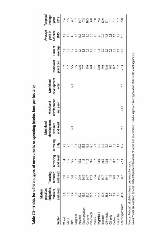
Tabl
e 7.8—
Yield
s for
diff
eren
t typ
es o
f inv
estm
ents
or s
pend
ing
(met
ric to
ns p
er h
ecta
re)
Mo
dern
pr
actic
es
Ma
rshl
and
Aver
age
Targ
eted
(ir
rigat
ion,
Te
rracin
g,
deve
lopm
ent,
Mars
hlan
d Ma
rshl
and
yield
in
aver
age
fe
rtiliz
er,
ferti
lizer
, Te
rracin
g Te
rracin
g fe
rtiliz
er,
deve
lopm
ent
deve
lopm
ent
Trad
ition
al Cu
rrent
ba
selin
e, yie
ld,
Sect
or
and
seed
) an
d se
ed
and
seed
on
ly an
d se
ed
and
seed
on
ly pr
actic
es
aver
age
2015
20
15
Whe
at 3.0
2.8
1.4
2.3
1.2
0.8
1.2
1.6Ma
ize
3.5
3.1
1.5
2.5
1.2
0.8
1.0
1.5
Rice
6.4
5.8
5.5
5.8
6.1
6.1
5.5
3.7
4.9
4.7So
rghu
m 3.4
2.7
1.7
2.4
1.5
1.1
1.5
1.7Po
tatoe
s 27
.2 24
.9 15
.5 20
.2
12.6
9.1
11.9
14.7
Swee
t pota
toes
15.0
16.8
11.2
11.5
7.7
5.5
6.9
7.8
Cass
ava
27.3
24.7
11.2
18.8
8.6
6.2
8.0
10
.5Ot
her r
oots
24.5
17.3
9.6
12.3
6.8
4.9
6.0
6.8
Pulse
s 2.7
2.4
1.2
2.1
1.1
0.8
1.0
1.0Ve
getab
les
29.5
19.6
14.0
19.6
14
.0 9.4
7.3
9.4
Bana
nas
17.9
15.7
10.5
14.9
9.9
7.2
10
.0 12
.9Ot
her f
ruits
28
.6 19
.1 13
.6 19
.1
13.6
9.7
14.3
17.1
Oilse
eds
2.7
1.8
1.1
1.4
0.8
0.6
0.8
1.1
Coffe
e 1.0
0.8
0.7
0.8
0.7
0.7
1.1
1.1Gr
een t
ea
1.7
1.4
1.2
1.4
1.2
1.1
1.7
1.7
Othe
r exp
ort c
rops
45
.8 38
.2 27
.3 38
.2 32
.7 23
.8 32
.7 27
.3 17
.6 26
.5 35
.0
Sour
ce: A
uthor
s’ ca
lculat
ions b
ased
on va
rious
liter
ature
.No
tes: Y
ields
are w
eighte
d by a
reas
with
diffe
rent
comb
inatio
ns of
inpu
ts an
d inv
estm
ents.
See
d = im
prov
ed se
ed ap
plica
tion.
Blan
k cell
s = no
t app
licab
le.
196 XINSHEN DIAO ET AL.
modern technology will be quite high; for example, maize can reach 3.5 metric tons per hectare (mt/ha) and potatoes 27 mt/ha. Although such yields seem to be at the maximum possible, when they are weighted by the corresponding land allocation reported in Table 7.7b, the effect on the national average yield is quite small, as only about 4.7 percent of total cropland (see the fi nal row of Table 7.7b) is expected to achieve such high levels of yield with the application of modern technology and in-puts. Moreover, more than 70 percent of cropland will still be without access to modern inputs by 2015, and yields achieved with traditional technology will still play a domi-nant role in determining the national average yields for most crops at that time.
As shown in the last column of Table 7.8, yields from most crops will continue to be low in 2015, even after signifi cantly increased public investment in agriculture. For example, the average maize yield at the country level is expected to be only around 1.5 mt/ha by 2015, although it is possible to have a yield of 3.5 mt/ha with a combination of irrigation, fertilizer, and improved seeds (see the fi rst column of Table 7.8). Although it is a signifi cant increase from the current level of maize yield of 0.8 mt/ha, this value is still lower than the maize yields already achieved by many Sub-Saharan African countries. To compare the current level of yield and possible yields by 2015 under the business-as-usual assumption, we report in the last three columns of Table 7.8 three different levels of national average yields. The yield level reported in the “Current average” column of Table 7.8 is consistent with the base-year yields applied in the model. Those numbers in the Table 7.8 column for the average yield in baseline, 2015, are consistent with those in the Table 7.2a column for yield in 2015. The numbers reported in the last column of Table 7.8 can be understood as the targeted average yield by 2015: the expected results with all planned public investment implemented.
Targeted crop average yields and the outcome of public investment in livestock and roads are applied in the DCGE model as exogenous shocks to land productivity (in the case of crop production) or total factor productivity (in the case of livestock production, trade, transportation, and communication sectors). Ideally, the DCGE model should consider all these different types of technologies to endogenously capture the productivity growth at the national level as a result of technology shifting from low to high yields. However, constrained by a lack of such information at the district level and between different types of farm groups (the production functions are defi ned at the district level for small and medium–large farms in the model), we are unable to capture the endogenous productivity growth in the analysis. Instead, we have to apply the exogenous productivity shocks calculated from the potential growth in the yields as results of public investments and use of modern inputs. With such exogenous shocks, the DCGE model generates a series of results that are in general consistent with the planned public investment and its targets. Because of this consistency, we do not need to report the model results of crop yield again.
RWANDA 197
We focus on the calculation of dollar-to-dollar returns to public investment in agriculture for this discussion. We measure such returns by increased GDP and AgGDP in real terms (that is, in terms of the base-year prices). To do this, we also consider future returns after 2015 from additional investment occurring in the next nine years. To calculate such future returns, we apply a 10 percent social discount rate and choose a long time period, such that for a given amount of public invest-ment combined with recurrent spending, the returns are eventually discounted to close to zero over the period chosen (for example, 20–30 years). We include spend-ing related to fertilizer and seed subsidies in the recurrent spending, which is also discounted with the same 10 percent social discount rate over the same period. As mentioned earlier, returns to public funds invested in a specifi c sector should not be measured narrowly by the benefi ts accrued to this sector. Because they are public goods, public investments often generate strong and positive externalities in the economy, such as technological spillovers in agriculture and growth linkages between agricultural and nonagricultural activities. Thus, increases in GDP over time (dis-counted to the current value) are used to measure the returns to agricultural invest-ment in Table 7.9, allowing us to fully capture the economywide gains of public investment in agriculture.
It is also important to measure the economywide returns as results of public funds invested in a specifi c agricultural subsector to understand which sectors yield more effi cient returns to investment. For this purpose, we designed a series of model scenarios, each of which focused on the investment going to a specifi c sector. For example, the fi rst row of Table 7.9 is the result of public funds invested in maize production. In this scenario we assume that productivity growth in maize production is the only direct outcome of increased investment, holding productivity growth in all other sectors at their baseline levels. Similarly, the second row of Table 7.9 assumes that only productivity growth in rice production comes directly from public investment. We also consider the productivity growth for groups of commodities, such as grains or root crops, as the results of public investment. For the “Grains” row, the result is from a scenario in which public investment directly results in the increase of yield in grain production, including maize, rice, wheat, and sorghum, while productivity growth in the other sectors is the same as in the baseline. The last two rows of Table 7.9 display results from the two scenarios considering broad investment in all agricultural subsectors. The second row from the bottom of this table shows that productivity growth in staple crops and livestock is the result of public investment while holding productivity growth in export crops at the baseline level; the last row of the table displays agricultural investments in all subsectors.
The fi rst column of Table 7.9 calculates returns to GDP for each unit of increased public funding invested in the agricultural sector or its subsectors. These returns are equivalent to benefi t–cost ratios. The second column of Table 7.9 reports
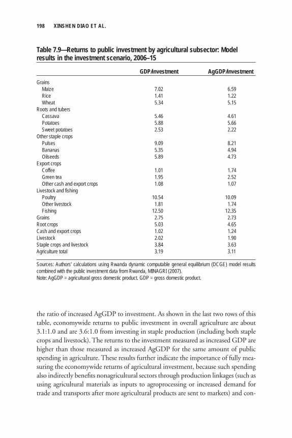
198 XINSHEN DIAO ET AL.
the ratio of increased AgGDP to investment. As shown in the last two rows of this table, economywide returns to public investment in overall agriculture are about 3.1:1.0 and are 3.6:1.0 from investing in staple production (including both staple crops and livestock). The returns to the investment measured as increased GDP are higher than those measured as increased AgGDP for the same amount of public spending in agriculture. These results further indicate the importance of fully mea-suring the economywide returns of agricultural investment, because such spending also indirectly benefi ts nonagricultural sectors through production linkages (such as using agricultural materials as inputs to agroprocessing or increased demand for trade and transports after more agricultural products are sent to markets) and con-
Table 7.9—Returns to public investment by agricultural subsector: Model results in the investment scenario, 2006–15
GDP/investment AgGDP/investmentGrains Maize 7.02 6.59 Rice 1.41 1.22 Wheat 5.34 5.15Roots and tubers Cassava 5.46 4.61 Potatoes 5.88 5.66 Sweet potatoes 2.53 2.22Other staple crops Pulses 9.09 8.21 Bananas 5.35 4.94 Oilseeds 5.89 4.73Export crops Coffee 1.01 1.74 Green tea 1.95 2.52 Other cash and export crops 1.08 1.07Livestock and fishing Poultry 10.54 10.09 Other livestock 1.81 1.74 Fishing 12.50 12.35Grains 2.75 2.73Root crops 5.03 4.65Cash and export crops 1.02 1.24Livestock 2.02 1.90Staple crops and livestock 3.84 3.63Agriculture total 3.19 3.11
Sources: Authors’ calculations using Rwanda dynamic computable general equilibrium (DCGE) model results combined with the public investment data from Rwanda, MINAGRI (2007).Note: AgGDP = agricultural gross domestic product. GDP = gross domestic product.
RWANDA 199
sumption linkages (because of farmers’ increased demands for nonagricultural goods stemming from their increased incomes).
At the aggregated subsector group level (see the second part of Table 7.9), returns to investment in root crops are highest, measured either as increased GDP or AgGDP. Returns to investment in grain production rank second, and returns to investment in export crops are the lowest but are still greater than one. The fi rst part of Table 7.9 reports economywide returns to investments in each agricultural sector’s production. For all agricultural sectors, returns to investment, measured by increased GDP, are greater than the cost of the investment, as all the numbers are greater than one and many are greater than two or three. However, in the case of coffee, returns to investment are the lowest, at 1.00 to 1.01. In contrast, coffee investment is quite profi table when measured directly by increased AgGDP, as RWF1 of investment results in RWF1.74 increase in AgGDP over time. That the increased GDP is sig-nifi cantly less than the increased AgGDP indicates the weak linkage of the coffee sector with the rest of economy. Coffee is grown mainly for export, and coffee pro-cessing is dominated by a simple process. Without increasing the value addition of coffee production, the sector is unlikely to create strong linkages and multiplier effects in the economy. Moreover, export-led growth can have certain macro-economic effects on the real exchange rate. For example, if growth in exports of primary products, including primary processed agricultural products (such as coffee and tea) is too high, it may cause the real exchange rate in the country to rise. An appreciated exchange rate could in turn raise the cost for other exportable sectors and make them more diffi cult to export. An appreciated exchange rate causes imports to become cheaper and thus import-competitive sectors become unable to compete. This is the other important factor explaining why returns to investment in coffee, measured by increases in GDP, are so low.
ConclusionsUnderstanding alternative agricultural growth options and their linkages with pov-erty reduction and prioritizing agricultural investments are the two key components of any agricultural development strategy. However, the relationships between growth and poverty reduction and between targeted growth and required public investment are not straightforward. Solid research is needed to support evidence-based policy-making and strategy formulation. This chapter provides such a study using Rwanda as the case country. The economywide DCGE model discussed in Chapter 2 was applied to the most recent economic data and public investment information to analyze the agricultural growth and investment options for poverty reduction in Rwanda. The analysis focuses on the linkages and trade-offs between growth and poverty reduction goals at the macro-, meso-, and microeconomic levels. It addresses
200 XINSHEN DIAO ET AL.
three policy-related questions: (1) What are the most effective pro-poor agricultural growth options? (2) How can the important linkages between agriculture and nonagriculture be strengthened so that nonfarm activities will become an important source of income for both growth and poverty reduction? (3) What are the most cost-effective public investment choices for stimulating shared growth and poverty reduction? The following key messages can be drawn from its analysis.
Accelerated Agricultural Growth Is Both Necessary and AchievableLow agricultural productivity and its interaction with environmental sustainability as the most severe challenge to Rwandan agriculture and rural development has been widely recognized both by researchers and the government. Productivity-led growth in agriculture is a key component of the country’s development strategy to deal with such challenges, and a series of targets has also been included in the strategy. The DCGE model simulations of this study indicate that the country’s targeted agricul-tural subsector growth, if achieved, would allow Rwanda to meet the CAADP target of 6 percent AgGDP growth from 2008 to 2015. With comparable growth in the nonagricultural sector, the agricultural growth would increase to 6.5 percent and total GDP growth to 7.4 percent, as a result of economywide linkages. The model also analyzes the linkages of this growth with the poverty reduction target of the strategy. Such growth would decrease the national poverty rate to 35.5 percent by 2015, a reduction of 24.8 percentage points over the 1999 rate. If this level of growth were to continue to 2020, Rwanda would be able to achieve the fi rst MDG of halving its national poverty rate by 2020, a target included in the country’s Vision 2020 (MINECOFIN 2000) and EDPRS (MINECOFIN 2008).
The Pattern of Subsector Growth Matters Agriculture comprises different activities, and export subsectors have often attracted more attention than other subsectors in many African countries’ agricultural strate-gic plans. Stemming from the belief that export-oriented subsectors can contribute more to the agricultural transformation, these subsectors have also disproportionally attracted more public resources and favorable policies. A similar policy bias also exists in Rwanda. Thus, it is necessary to understand the role of different types of agricultural subsectors in both growth and poverty reduction to help prioritize public investment and agricultural policy. The DCGE model discussed in this chapter includes detailed agricultural activities as individual subsectors as well as a broad range of many nonagricultural activities. Through linkages between agriculture and non-agriculture and among agriculture both in production and consumption processes, the DCGE model simulations show that most rural households would benefi t from rapid but broad-based agricultural growth and the distribution of such benefi ts is comparatively equal. However, the most vulnerable households—those with
RWANDA 201
extremely small landholdings and few opportunities to participate in the production of cash crops—appear to benefi t less.
Analyzing the linkages between subsector-level growth and poverty reduction is one of the important contributions of this study, and such an analysis is carried out by endogenously measuring the poverty-reduction response to the economy-wide growth led by different sectors. This chapter fi rst compares the poverty-reduction effect of growth led by the agricultural sector versus that led by the non-agricultural sector, and the model results show that each 1 percent of growth in per capita GDP, driven by agriculture, has a much greater effect on poverty reduction than does the same level of growth driven by the nonagricultural sector. The chapter further compares the subsectors’ roles in poverty reduction by simulating economy-wide growth led by different agricultural subsectors. The simulation results indi-cate that overall growth driven mainly by increased productivity in staple crops has the greatest effect on poverty reduction. Agricultural households with greater opportunities to produce high-value export products are better positioned to bene-fi t from export agriculture. But these households are usually not as poor as other, more remote, households, so export-led growth may have less impact on reducing poverty.
The roles of different agricultural subsectors in economic development are also analyzed from other aspects. Cereals, especially rice and maize, are among the high priorities in the government’s strategy document; accordingly, they have high growth targets. If these growth targets are reached, cereals would become the most impor-tant source of income growth for many rural households, especially for those with relatively small landholdings. Results of the report also show that food security does not equal food self-suffi ciency. Although growth in cereals would help the country reduce its dependence on imports, both maize and rice will continue to depend on imports, but the ratio of imports to domestic consumption will signifi cantly fall by 2015. In contrast, export agriculture is important because of its contribution to macroeconomic balance in trade. High growth in both traditional and non-traditional agricultural exports is targeted in the government’s strategy, and the model shows that such growth would signifi cantly increase agricultural trade sur-pluses. The projected agricultural trade surplus would be about 29 percent of the nonagricultural trade defi cit, more than three times the current ratio.
This chapter also warns of possible price declines in some commodities with very high growth targets. Unbalanced growth does not always benefi t producers if it is concentrated in a few subsectors. As the targeted growth rates for some livestock products (such as poultry and raw milk) are very high, a negative price effect could result if production growth is out of balance with income growth. Simulations indicate that with an annual growth in poultry production of more than 9 percent and in raw milk more than 15 percent during 2007–15, prices for these two com-
202 XINSHEN DIAO ET AL.
modities will decline 35–40 percent, even though their demand is highly income elastic.
More Agricultural Expenditure and Higher Spending Efficiency Are Needed Required public investment in agriculture is calculated in this chapter according to the growth needed to meet the CAADP agricultural growth goal of 6 percent or the fi rst MDG by 2020. The effi ciency of spending, which is captured by the elasticity of agricultural growth to spending, affects the amount and growth of agricultural spending. This chapter shows that meeting the CAADP growth target will require allocation of public resources to the agricultural sector to rise to 10.0–17.6 percent of total spending by 2015, where the lower value refl ects a higher growth–spending elasticity (that is, more effi ciency in spending) and the higher value refl ects a lower elasticity. These levels of allocation translate, in real terms, to 15 and 30 percent annual growth in agricultural spending. Given that agriculture needs to grow at 6.5 percent to meet the goal of halving the national poverty rate by 2020, more rapid growth in agricultural spending between 2008 and 2015 is required. Our result in terms of required agricultural spending, using the high elasticity that represents an average standard for the Sub-Saharan Africa as whole, is consistent with the CAADP target, which requires a minimum of 10 percent of the government budget to be allocated to agricultural spending. This result is also consistent with the original cost estimation prepared by MINAGRI without scaling down because of the constraints set by the Rwandan Ministry of Finance. Such a spending pattern seems to be neces-sary both for achieving more than 6 percent agricultural annual growth and for helping the country meet the target set in Vision 2020 for halving poverty by 2020. Of course, effi ciency of public spending must also improve.
Economywide Returns to Public Investment in Agriculture Are HighFor an agricultural strategy that can be practically implemented, it is necessary to understand what can be done in addition to what should be done. To help under-stand the fi rst part of this issue, returns to public investment in agriculture need to be analyzed. Most cost–benefi t analyses are at the micro or project level, which may signifi cantly underestimate the returns to public investment, because such invest-ments generally have impacts going beyond the targeted sector or project. One of the important contributions of this chapter is to measure such returns from an economywide perspective. Although the approach used in the measure is ex ante because of a lack of past investment data for a sound econometric estimation, the measurement results are informative for prioritizing public investment. Our analysis fi nds that, measured as increased GDP over time, the economywide return to agri-cultural investment (the benefi t–cost ratio) is 3.2:1.0. Part of such gains comes from
RWANDA 203
growth in the nonagricultural sector as a result of multiplier and linkage effects between agriculture and nonagriculture. Comparing increased GDP with increased AgGDP as the outcomes of RWF1 of additional public investment in agricultural staples, we see that increased GDP is RWF0.21 more than that of AgGDP, indicat-ing that returns to agricultural investment stimulates growth in the nonagricultural sector.
The Highest Economywide Returns from Investment Are from Staple CropsUsing an approach similar to that discussed above, our study also measures returns to agricultural investments in different agricultural subsectors. The results show that economywide returns to public investment in staple crop production are the highest of all sectors. Spending on root crops is particularly effi cient. Given that both current yields and the use of modern inputs are extremely low for most grain and root crops (except for rice) in Rwanda, even compared to other Sub-Saharan African countries, the country needs to give a much higher priority to these crops than is usual. The high returns are also the result of a linkage effect, particularly for root crops, as pro-ductivity growth in such crops lowers pressure on land expansion, which is an extremely important factor that must be taken into consideration in any agricultural strategy for Rwanda. Staple crops are broadly consumed by poor consumers in both rural and urban areas, and reduced food prices from productivity-led growth benefi t the poor consumers and create more growth opportunities in other agricultural and nonagricultural sectors. However, the amount of investment specifi ed in EDPRS (Rwanda, MINECOFIN 2008) will not be enough to signifi cantly improve the low yields of many crops nationwide. The average yield for maize will be as low as 1.5 mt/ha even in 2015, a level many African countries have already reached.
Trade-Offs Exist between Exports and Overall Growth When Investing in Export CropsAlthough investment in export crops has the highest impact on growth in these subsectors, the economywide returns are quite low. The growth rate of coffee and tea can reach double digits with targeted investment to the export sector, measured by increased GDP over time; however, such investment has the lowest returns of all sectors, particularly in the case of coffee. The reason for these low returns is mainly due to the weak linkages with other economic activities both on the production and consumption sides. It is possible to strengthen such linkage effects in the export sector by promoting agroprocessing with high-value addition (because of weak income–consumption linkages), but the same amount of public investment in the export sector is not likely to become a dominant driver for both overall economic growth and poverty reduction.
204 XINSHEN DIAO ET AL.
In many African countries the export sector has often attracted more govern-ment attention than have other sectors. With favorable policies and investment support, government spending to promote the export sector represents a much higher share of total agricultural spending, compared to the size of the export sector in the total agricultural economy. The fi ndings of this chapter show relatively low economywide returns to public spending in the export sector and relatively less poverty reduction from growth led by promoting exports, further indicating the importance of broad-based agricultural growth. Agricultural development strategy, including an effective public investment strategy, should focus more on growth in which a majority of farmers can participate. Only such a strategy can be expected to be effi cient and effective in growth and poverty reduction, as well as in the eco-nomic development of the country in general.
How Relevant Is the Rwandan Case to Other African Countries?Although Rwanda is one of the smallest countries and has the highest population density in Africa, similarities do exist between Rwanda and many other African countries. First, it is true that at the country level, fewer African countries have such high population pressure in economic development as in Rwanda. Constrained by the lack of additional arable land to support high population growth, to develop an effi cient agricultural system whose growth is productivity driven and sustainable environmentally is more urgent in Rwanda than in other African countries. However, because of recent rapid increases in population throughout the continent, many countries have started to feel similar pressure from population growth on agricultural development either at the country or subnational level. Such countries as Ethiopia, Kenya, and Malawi face similar constraints in their high-population areas, and such areas are often the food baskets of their respective countries. Environment degradation (such as soil erosion and deforestation stemming from extensive farming systems) is commonly observed in certain areas of almost all African countries, even in the countries with relatively abundant land, such as Ghana and Nigeria. Thus, challenges facing Rwanda’s agriculture today are becoming challenges facing agricultural development in many other African countries today or in the near future. From this point of view, the analysis discussed in this chapter is highly relevant to many African countries in terms of their agricultural development strategies.
Second, agriculture is once again becoming a top priority on the agenda in economic development strategy for all African countries. As a result, an understand-ing of the linkages in growth across agricultural subsectors and between agriculture and nonagriculture and the linkages between growth and poverty reduction is com-monly required for designing an agricultural strategy. Although such understanding has to be country specifi c, the methodology developed in this chapter, which takes
RWANDA 205
an economywide perspective, is useful for many countries. The general principles that this chapter emphasizes—such as to link agricultural subsectors’ targets to overall growth and poverty reduction, to understand the different roles of different subsectors in growth and poverty reduction at the macro- and microlevels, and to pay attention to certain trade-offs and negative effects (such as price effects) of rapid and unbalanced growth—are all relevant to other countries when designing their development strategies.
Third, almost all African countries are facing constraints on their public resources for supporting agricultural growth. The fi nancial gap between what should be done and what can been done is commonly seen in many country’s development strategy documents. By calculating the public spending required for achieving the targets set by the strategy documents, this chapter explicitly measures such gaps and points out that their acknowledgment has to be a part of any development strategy. The chapter emphasizes the relationship between the effi ciency in spending and the amount of spending required to support agriculture, which is a common challenge facing many African countries. As in Rwanda, a commonly observed constraint in many African countries is that, because of a lack of suffi cient data and information for a reasonable econometric analysis, the returns to public investment are unlikely to be measured at the sector level to better prioritize public investment. This chapter describes a new approach (though it is ex ante) that is able to fully use the informa-tion available in a country’s PRSP preparation process. This approach can be adopted in other countries’ strategic studies.
Finally, research on development strategy at the country level in Africa is a new fi eld in today’s political environment. As more and more countries defi ne their agricultural development strategies and almost all these strategies are dynamic documents to be improved and updated over time, the needs for evidence-based development-strategy research are high and demand is rising. However, researchers in this fi eld are facing challenges stemming from a lack of solid data and feel the urgency to provide research outcomes in a relative short period of time to meet policy demand. Although the analysis presented in this chapter is far from perfect, it is an encouraging attempt to make development research more relevant to developing countries’ policies and strategies.
206 XINSHEN DIAO ET AL.
Appendix
Table 7A.1—Structure of the Rwandan social accounting matrix
Agricultural sectors Wheat; maize; rice; sorghum; potatoes; sweet potatoes; cassava; other roots; pulses; vegetables; bananas; other fruits; oilseeds; export crops; coffee; tea; other export
crops; cattle; sheep and goats; swine; poultry; raw milk; eggs; other livestock products; forestry; fishing
Industrial sectors Mining; meat, fish, and dairy products; processed cereals; processed coffee; processed tea; bakery and processed sugar; traditional beverages; modern beverages;
tobacco; textiles and clothing; wood, paper, and printing; chemicals; nonmetallic minerals; furniture and other manufactured products; electricity, gas, and water; construction
Service sectors Wholesale and retail trade; hotels and restaurants; transport; communications; finance and insurance; real estate; business services; repair; public administration;
education; health; other personal servicesFactors Unskilled agricultural labor; unskilled nonagricultural labor; skilled labor; agricultural land (by regions); agricultural capital; nonagricultural capital Households Farm households by region (60 in total); nonfarm households (2 in total)Regions Administrative districts for agriculture only (30 districts in total further disaggregated into small farms and medium–large farms)
Source: Authors.
Notes 1. Seven percent of total planned public spending between 2008 and 2012 will be allocated to agriculture in EDPRS. 2. According to Kelly et al. (2001b), 5 percent of farmers used inorganic fertilizers or lime (or both) on 3 percent of cultivated land during the 2000 season. However, as we assume that fertilizer is used at the recommended level, the number reported in Tables 7.7a and 7.7b for fertilized land as a share of cultivated land is smaller than what was reported by Kelly et al.
ReferencesAkita, T., and M. Kawamura. 2002. “Regional Income Inequality in China and Indonesia: A
Comparative Analysis.” Paper presented at the 42nd Congress of the European Regional Science
Association, Dortmund, Germany, August 27–31.
Arnault, E. C. 2007. “The 2006 Social Accounting Matrix of Rwanda: Methodology Note.”
Unpublished memo, University of Yaounde II, Yaounde, Cameroon.
Bezemer, D., and D. Headey. 2008. “Agriculture, Development and Urban Bias.” World Development
34 (8): 1342–1364.
Bigsten, A., and A.-S. Isaksson. 2008. Growth and Poverty in Rwanda: Evaluating the EDPRS 2008–
2012. Country Economic Report 2008:3. Department for Policy and Methodology, Swedish
International Development Agency. Stockholm, Sweden. www.sida.se/publications.
RWANDA 207
Blarel, B., P. Hazell, F. Place, and J. Quiggin. 1992. “The Economics of Farm Fragmentation: Evidence
from Ghana and Rwanda.” World Bank Economic Review 6 (2): 233–254.
Byerlee, D., X. Diao, and C. Jackson. 2005. “Agriculture, Rural Development, and Pro-Poor Growth:
Country Experiences in the Post-Reform Era.” Input paper for the project “Operationalizing
Pro-Poor Growth in the 1990s.” Washington, DC: World Bank.
Chen, S., and M. Ravallion. 2000. How Did the World’s Poorest Fare in the 1990s? Policy Research
Working Paper 2409. Washington, DC: World Bank.
Clay, D. C. 1996. Fighting an Uphill Battle: Population Pressure and Declining Land Productivity in
Rwanda. International Development Working Paper 58. East Lansing, MI, US: Department of
Agricultural Economics, Michigan State University.
Clay, D. C., F. Byiringiro, J. Kangasniemi, T. Reardon, B. Sibomana, L. Uwamariya, and D. Tardif-
Douglin. 1995. Promoting Food Security in Rwanda through Sustainable Agricultural Productivity:
Meeting the Challenges of Population Pressure, Land Degradation and Poverty. International
Development Paper 17. East Lansing, MI, US: Department of Agricultural Economics, Michigan
State University.
Collier, P. 2003. “Primary Commodity Dependence and Africa’s Future.” In Annual World Bank
Conference on Development Economics 2003: The New Reform Agenda, edited by B. Pleskovic and
N. Stern, 139–162. Washington, DC; New York: World Bank; Oxford University Press.
Diao, X., P. Hazell, and J. Thurlow. 2010. “The Role of Agriculture in African Development.” World
Development 38 (10): 1375–1383.
Diao, X., P. Hazell, D. Resnick, and J. Thurlow. 2007. The Role of Agriculture in Development:
Implications for Sub-Saharan Africa. Research Report 153. Washington, DC: International Food
Policy Research Institute.
Diao, X., S. Fan, S. Kanyarukiga, and B. Yu. 2010. Agricultural Growth and Investment Options for
Poverty Reduction in Rwanda. Research Monograph. Washington, DC: International Food Policy
Research Institute.
Ellis, F. 2005. “Small Farms, Livelihood Diversifi cation, and Rural–Urban Transitions: Strategic Issues in
Sub-Saharan Africa.” In The Future of Small Farms: Proceedings of a Research Workshop, Wye, U.K.,
June 26–29, 2005, 135–149. Washington, DC: International Food Policy Research Institute.
Fan, S., B. Yu, and A. Saurkar. 2008. “Public Spending in Developing Countries: Trends, Determination
and Impact.” In Public Expenditures. Growth and Poverty: Lessons from Developing Countries, edited
by S. Fan. Baltimore: Johns Hopkins University Press.
Fleskens, L. 2007. Prioritizing Rural Public Works Interventions in Support of Agricultural Intensifi cation:
Annex Report. Kigali, Rwanda: Helpage Rwanda; Catalyze Accelerated Agricultural Intensifi cation
for Social and Environmental Stability, International Center for Soil Fertility and Agricultural
Development (IFDC).
Fowler, M., C. Gasirabo, S. Kanyarukiga, and A. Mutijima. 2007. “Rwanda Public Expenditure
Review—Agriculture.” Report for the Ministry of Agriculture and Animal Resources, Rwanda.
208 XINSHEN DIAO ET AL.
Accessed February 2, 2012. www.amis.minagri.gov.rw/content/rwanda-public-expenditure-
review-agriculture-2007.
Haggblade, S., P. Hazell, and T. Reardon. 2007. “Strategies for Stimulating Equitable Growth in the
Rural Nonfarm Economy.” In Transforming the Rural Nonfarm Economy, edited by S. Haggblade,
P. B. R. Hazell, and T. Reardon, 396–416. Baltimore: Johns Hopkins University Press.
IMF (International Monetary Fund). 2004. Rwanda: Selected Issues and Statistical Appendix. Country
Report 04/383. Washington, DC.
Johnson, M., P. Hazell, and A. Gulati. 2003. “The Role of Intermediate Factors Markets in Asia’s Green
Revolution: Lessons for Africa?” American Journal of Agricultural Economics 85: 1211–1216.
Kanbur, R., and X. Zhang. 2004. Fifty Years of Regional Inequality in China: A Journey through Revolution,
Reform, and Openness. Research Paper 2004/50. Helsinki, Finland: World Institute for Develop-
ment Economics Research, United Nations University.
Kelly, V., E. Mpyisi, E. Shingiro, and J. B. Nyarwaya. 2001a. Agricultural Intensifi cation in Rwanda: An
Elusive Goal. Fertilizer Use and Conservation Investment. International Development Collaborative
Policy Brief RW-FSRP-PB-01. East Lansing, MI, US: Department of Agricultural Economics,
Michigan State University.
Kelly, V., E. Mpyisi, A. Murekezi, and D. Neven. 2001b. “Fertilizer Consumption in Rwanda: Past
Trends, Future Potential, and Determinants.” Paper presented at the Policy Workshop on Fertilizer
Use and Marketing, Kigali, Rwanda, February 22–23.
King, R. P., and D. Byerlee. 1978. “Factor Intensities and Locational Linkages of Rural Consumption
Patterns in Sierra Leone.” American Journal of Agricultural Economics 60 (2): 197–206.
Lopez, H., and Q. Wodon. 2005. “The Economic Impact of Armed Confl ict in Rwanda.” Journal of
African Economies 14 (4): 586–602.
Maxwell, S., and R. Slater. 2003. “Food Policy Old and New.” Development Policy Review 21 (5–6):
531–553.
Ndulu, B., and S. O’Connell. 2006. “Policy Plus: African Growth Performance 1960–2000.” In The
Political Economy of Economic Growth in Africa 1960–2000, edited by B. Ndulu, S. O’Connell,
R. Bates, P. Collier, and C. Soludo, 3–75. Cambridge, UK: Cambridge University Press.
NISR (National Institute of Statistics Rwanda). 2006. Preliminary Poverty Update Report: Integrated
Living Conditions Survey 2005/06. Kigali, Rwanda: Republic of Rwanda.
REMA (Rwanda Environment Management Authority). 2009. Rwanda State of Environment and
Outlook Report. Kigali, Rwanda.
Roose, E., and F. Ndayizigiye. 1997. “Agroforestry, Water and Soil Fertility Management to Fight
Erosion in the Tropical Mountains of Rwanda.” Soil Technology 11: 109–119.
Rwanda, MINAGRI (Ministry of Agriculture, Animal Resources and Forestry, Rwanda). 2004a.
National Agricultural Policy. Kigali, Rwanda: Republic of Rwanda.
RWANDA 209
———. 2004b. Strategic Plan for Agricultural Transformation in Rwanda, Main Document. Kigali,
Rwanda.
———. 2007. Unpublished Statistics Data Files. Excel fi le, Republic of Rwanda, Kigali, Rwanda.
———. 2008. “Total Cost of EDPRS Agricultural Sector.” Mimeo, Kigali, Rwanda.
Rwanda, MINECOFIN (Ministry of Finance and Economic Planning, Rwanda). 2000. Vision 2020.
Kigali, Rwanda.
———. 2002. Poverty Reduction Strategy Paper. Kigali, Rwanda.
———. 2003. Household Living Conditions Survey, 1999/2001. Kigali, Rwanda.
———. 2007. Household Living Conditions Survey, 2005/2006. Kigali, Rwanda.
———. 2008. Economic Development and Poverty Reduction Strategy, 2008–2012. Kigali, Rwanda.
Thirtle, C., L. Lin, and J. Piesse. 2003. “The Impact of Research-Led Agricultural Productivity Growth
on Poverty Reduction in Africa, Asia and Latin America.” World Development 31 (12):
1959–1975.
Verpoorten, M., and L. Berlage. 2004. “Genocide and Land Scarcity: Can Rwandan Rural Households
Manage?” Forum paper for The African Development and Poverty Reduction: The Macro–Micro
Linkage, Somerset West, South Africa, October 13–15.
Verwimp, P. 2003. “Testing the Double-Genocide Thesis for Central and Southern Rwanda.” Journal
of Confl ict Resolution 47: 423–442.
Von Braun, J., H. de Haen, and J. Blanken. 1991. Commercialization of Agriculture under Population
Pressure: Effects on Production, Consumption, and Nutrition in Rwanda. Research Report 85.
Washington, DC: International Food Policy Research Institute.
World Bank. 2008a. World Development Indicators. Washington, DC.
———. 2008b. World Development Report 2008: Agriculture for Development. Washington, DC.

C h a p t e r 8
NigeriaXinshen Diao, Manson Nwafor, Vida Alpuerto,
Kamiljon T. Akramov, Valerie Rhoe, and Sheu Salau
Nigeria, whose export earnings are heavily oil dependent, has experienced rapid economic growth in recent years. In 1990–99 the economy grew at 2.6–3.0 percent annually, whereas the annual gross domestic product (GDP)
growth rate rose to 7.3 percent during 2000–07 (Nigeria, NBS 2007a). Notably, the agricultural sector has been the key driver of the economy, growing at 6.3 percent and contributing 42 percent to the country’s total GDP in 2008. Hence, despite the high dependence of government revenues and national export earnings on the oil sector, the agricultural sector remains the country’s mainstay (Sanyal and Babu 2010). Furthermore, because agriculture is the largest employer among all sectors (70 percent of the labor force) (Nigeria, NBS 2006) and labor is the main (and sometimes only) asset for the poor (Agenor Izquierdo, and Fofack 2003), the agri-cultural sector has the greatest potential for reducing poverty.
Nigeria has undergone a painful process before it recently recognized the importance of the agricultural sector in its development process. Although the agri-cultural sector received some policy attention immediately after the country’s in-dependence, the oil boom in the early 1970s eventually pushed the country toward a development crisis, with many years of civil confl ict and economic stagnation (and even recession). During this period, agriculture and rural development were largely ignored, poverty rose, food insecurity and malnutrition worsened, and the country turned from being a net agricultural exporter to a food importer by the end of the 1970s (World Bank 2010). By 1996, two-thirds of the country’s population lived in poverty, and the poverty rate almost tripled in the 15 years between 1980 and 1996 (World Bank 2010).
212 XINSHEN DIAO ET AL.
Drawing lessons from its troubled economic history, the Government of Nigeria has since recognized the importance of the agricultural sector. Its promotion is an essential ingredient of the country’s development strategy, given the country’s rich, favorable agroecological conditions and the fact that most of the population lives in rural areas. A series of strategies has recently been designed that aim to accelerate agricultural growth, strengthen food security, and reduce poverty. These strategies include the National Economic Empowerment and Development Strategies (NEEDS) (Nigeria, NPC 2004, 2007) and the National Food Security Program (NFSP) (Nigeria, FMARD 2008). Such programs as the presidential initiatives on cassava, rice, and other crops have also been implemented. Moreover, the country is a signa-tory to the Comprehensive Africa Agriculture Development Programme (CAADP), which commits the government to targeting 6 percent agricultural GDP growth rate and allocating at least 10 percent of public resources to the agricultural sector. Despite these commitments, further efforts are needed to lift more people out of poverty and to meet the fi rst Millennium Development Goal (MDG) of halving the proportion of the people living on less than US$1 a day.
In this chapter we analyze the agricultural growth and public investment options for Nigeria. This study provides evidence-based analysis to support the formation of a more comprehensive rural development component under the NEEDS that is also in alignment with the objectives collectively defi ned by African countries as part of the CAADP agenda. As with other chapters in this volume, the analysis makes use of a spatially disaggregated recursive dynamic computable general equilibrium (DCGE) model (described in Chapter 2). We also estimate the overall cost to the government of the investments needed to accelerate agricultural growth.
The chapter is structured as follows. We fi rst describe the structure of the Nigerian DCGE model and the data sources used to calibrate it. The model results are then presented for the baseline growth scenario and the accelerated agricultural growth scenarios. This is followed by the results from the investment analysis. The fi nal section draws together our fi ndings and summarizes their implications for future national and agricultural development strategies in Nigeria.
The Nigerian DCGE ModelThe Nigerian DCGE model includes 62 production subsectors that cover the entire agricultural and nonagricultural components of the country (see Table 8A.1 in the appendix to this chapter). More than half of the subsectors are in agriculture, which falls into six broad groups: cereal crops, root crops, other foodcrops, higher value export-oriented crops, livestock sectors, and other agricultural activities (that is, forestry and fi sheries). The model also captures regional heterogeneity in agriculture by disaggregating agricultural production into six zones, wherein representative farm-ers produce different crops and livestock across zones. In terms of nonagricultural
NIGERIA 213
activities, there are 10 agroprocessing activities, including 8 concerning food pro-cessing. On the demand side, the Nigerian DCGE model includes 12 household groups defi ned for the six zones and by rural and urban location. Each of the 12 household groups is aggregated from the Nigeria Living Standards Survey (NLSS) 2003/04 (Nigeria, NBS 2003) such that all sample households in NLSS are linked directly to their corresponding representative households in the DCGE model via the microsimulation module described in Chapter 2.
The data used to represent the base year of the model are drawn from a variety of data sources. The core dataset underlying the DCGE model is a 2006 social accounting matrix (SAM) constructed using national accounts and trade data, both of which were published by Nigeria’s National Bureau of Statistics (2008b), and balance-of-payment information, which was published by the Central Bank of Nigeria (CBN 2009). National and state agricultural production and yield data and market price data are obtained from the Federal Ministry of Agriculture and Rural Develoment (2009). When production data are unavailable for certain sectors (for example, horticulture), information is taken from FAO (2010). Agricultural pro-duction was disaggregated across zones by mapping individual states to the six zones. The DCGE model is therefore consistent with offi cial agricultural produc-tion levels and yields at the zonal level. Nonagricultural production, employment, and other value-added components of sectoral GDP at the national level were com-piled from national accounts. On the demand side, information on industrial technologies (for example, intermediate and factor demand) is taken from an earlier SAM for Nigeria developed by Iyaniwura et al. (1992) for a UNDP project, while the income and expenditure patterns for the various household groups are taken from NLSS 2003/04. The DCGE model is therefore based on the most recent data available for Nigeria and represents the country’s economy in 2006.
Baseline Growth ScenarioThe DCGE model is fi rst used to simulate a baseline scenario that captures current trends in growth and poverty reduction. History shows that the Nigerian economy is vulnerable to oil price shocks through impacts on the country’s effective exchange rate, government expenditure, money supply, trade, and infl ation (Akpan 2009). Given that the global fi nancial crisis and declines in world crude oil prices are expected to last for some time, a modest targeted economic growth of 6.5 percent per year for total GDP was assumed for the baseline during 2008–17. Although this targeted baseline growth rate is lower than Nigeria’s recent growth performance (for example, it was 7.6 percent annually during 2002–07), it is comparable with growth over a longer period (for example, the average annual GDP growth rate was 5.5 percent during 1995–2007). Similarly, a relatively modest growth rate of 5.7 percent
214 XINSHEN DIAO ET AL.
for the agricultural sector was assumed for the baseline, which is comparable to the historical growth rate during 2000–07.
Factors Determining Growth in the ModelTo model a realistic baseline, it is important to pay attention to the sources of growth across sectors and for different input factors. In the model, economic growth results from increases in labor supply, land expansion, capital accumulation, and productiv-ity changes. We assume that growth in total labor supply is consistent with projected growth in the population (that is, 3.0 percent annually). By taking into account more rapid growth in the nonagricultural sector’s labor demand, growth in the economywide labor categories (unskilled and skilled labor) is assumed to be 3.3 percent and 3.4 percent, respectively. A much slower growth rate of 2.0 percent annually is assumed for rural family labor supply. Total agricultural land expansion was also exogenously imposed on the model, based on recent trends reported by the National Planning Commission (2007) (that is, 5.2 percent per year). Land expan-sion is assumed to eventually fall to 4.2 percent after 2011, and thus the average annual growth rate of land expansion is 4.8 percent (Table 8.1). Because of a lack of information on the potential for land expansion at the zonal level, we assumed a uniform growth rate across the six zones.
Capital accumulation is an endogenous outcome of savings and investments, which are modeled recursively in our model (see Chapter 2). Investment is fi nanced through private savings determined by (1) a fi xed proportion of the total income (an endogenous variable) received by each of the 12 representative households and (2) government savings, which is a residue term between government income (an endogenous variable) and total noninvestment spending (an exogenous variable). Both private and public savings rates are calibrated to the 2006 SAM. Investment is also affected by the foreign capital fl ows. Because Nigeria has run a trade surplus in recent years, net foreign capital infl ows are negative in the model (which indicates capital outfl ows). In the DCGE model, such outfl ow is an exogenous variable, and growth of the outfl ows is assumed to decline from the expected slow growth in oil exports. Using this assumption, more oil revenues are expected to be used in fi nanc-ing domestic investment instead of purchasing foreign bonds or investing in foreign capital markets in the current situation. In the baseline, capital accumulates at 4.6 percent each year in real terms after 5.0 percent depreciation (see Table 8.1).
Although total factor supply grows either exogenously (labor and land) or endogenously (capital), demand at the sector level is endogenous. Factor demand is determined by the competiveness in factor markets and the profi tability of each individual sector. The third part of Table 8.1 reports the growth rate in aggregate labor and capital demand by agriculture and nonagriculture. The model results show that total agricultural labor demand grows at 2.2 percent annually, but it is 3.7
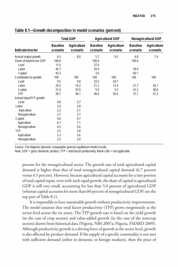
NIGERIA 215
percent for the nonagricultural sector. The growth rate of total agricultural capital demand is higher than that of total nonagricultural capital demand (6.7 percent versus 4.5 percent). However, because agricultural capital accounts for a tiny portion of total capital input, even with such rapid growth, the share of capital in agricultural GDP is still very small, accounting for less than 5.0 percent of agricultural GDP (whereas capital accounts for more than 60 percent of nonagricultural GDP; see the top part of Table 8.1).
It is impossible to have sustainable growth without productivity improvements. The model assumes that total factor productivity (TFP) grows exogenously at the sector level across the six zones. The TFP growth rate is based on the yield growth (in the case of crop sectors) and value-added growth (in the case of the noncrop sectors) drawn from historical data (Nigeria, NBS 2007a; Nigeria, FMARD 2009). Although productivity growth is a driving force of growth at the sector level, growth is also affected by product demand. If the supply of a specifi c commodity is not met with suffi cient demand (either in domestic or foreign markets), then the price of
Table 8.1—Growth decomposition in model scenarios (percent)
Total GDP Agricultural GDP Nonagricultural GDP
Baseline Agriculture Baseline Agriculture Baseline AgricultureIndicator/sector scenario scenario scenario scenario scenario scenarioAnnual output growth 6.5 8.0 5.7 9.5 6.8 7.4Share of total/sector GDP 100.0 100.0 100.0 Land 11.0 37.0 Labor 45.7 59.4 39.9 Capital 43.3 3.6 60.1 Contribution to growth 100 100 100 100 100 100 Land 9.5 9.8 33.3 24.7 Labor 20.2 16.2 21.2 12.4 21.7 20.1 Capital 31.6 25.9 5.0 3.3 41.2 38.6 TFP 38.7 48.1 40.6 59.6 37.1 41.2Annual input/TFP growth Land 4.8 5.7 Labor 3.0 3.0 Agriculture 2.2 2.1 Nonagriculture 3.7 3.7 Capital 4.6 4.7 Agriculture 6.7 7.1 Nonagriculture 4.5 4.6 TFP 2.5 3.8 Agriculture 2.3 5.6 Nonagriculture 2.5 3.0
Source: The Nigerian dynamic computable general equilibrium model results.Note: GDP = gross domestic product. TFP = total factor productivity. Blank cells = not applicable.
216 XINSHEN DIAO ET AL.
this commodity in the domestic market will fall, resulting in reduced factor demand by producers of this commodity (and hence a lower GDP growth rate).
We calculate the contribution of factors and productivity to the overall eco-nomic growth in Table 8.1. Factor contributions to GDP growth depend on the growth rate of each factor and the share of these factors in value-added. For the economy as a whole, land accounts for 11.0 percent of GDP, whereas labor and capital account for 45.7 percent and 43.3 percent, respectively. In terms of growth in GDP in the baseline scenario, 61.3 percent of growth is due to factor accumula-tion, whereas 38.7 percent comes from TFP growth (see the second part of Table 8.1). Growth contributions for agricultural and nonagricultural GDP are also reported in the table. In the baseline, almost 60 percent of agricultural growth is due to land expansion, increased labor supply, and capital accumulation, whereas productivity only explains 40 percent of growth. Within crop sectors, productivity gains come both from improvement in yields and a more effi cient allocation of land to crops with higher returns.
Growth at the Subsector LevelOverall growth in the baseline total and agricultural GDP is targeted at 6.5 percent and 5.7 percent, respectively, annually between 2009 and 2017, the growth rate is very different across individual subsectors. This is because the input allocation across sectors differs over time as a result of different sectoral productivity growth and changes in relative prices. For example, although agricultural GDP grows at 5.7 percent annually, growth in total cereal value-added is 5.4 percent (Table 8.2). It is 5.1 percent and 7.3 percent for rice and maize production, respectively, whereas growth in Irish potatoes is 8.8 percent annually. The table also presents baseline GDP growth by subsector, as well as for some sector groupings. All growth rates are endogenous results of the model. The fi rst column of the table reports the size of each sector as a share of total GDP in 2006.
Poverty-Reduction Outcome in the Baseline SimulationThe poverty-reducing impact of economic growth is analyzed using a micro-simulation module. Before the simulation exercise was started, the impact of growth on poverty reduction using historical poverty data available for 1980, 1985, 1992, 1996, and 2004 at the national level was assessed. However, because the poverty rate of 65.6 percent in 1996 is much higher than that in 1992 (42.7 percent), it makes the trend analysis diffi cult over a long period. For this reason, we focus on the pov-erty rate between 1996 (during which the poverty rate was 65.6 percent) and 2004 (54.4 percent) and compare the rates with actual per capita GDP growth over the same period. Although the annual growth rate of GDP per capita is 2.5 percent (calculated from an annual growth in GDP of 5.5 percent and population annual
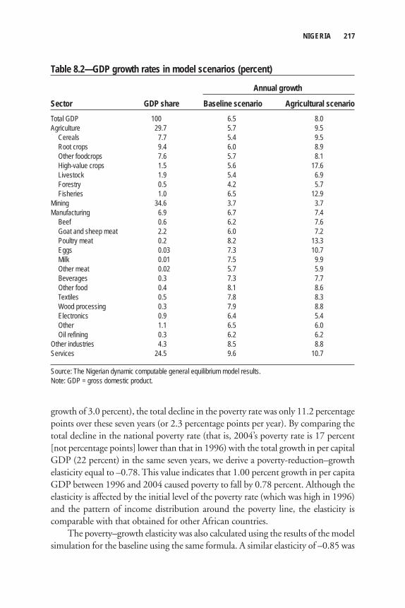
NIGERIA 217
growth of 3.0 percent), the total decline in the poverty rate was only 11.2 percentage points over these seven years (or 2.3 percentage points per year). By comparing the total decline in the national poverty rate (that is, 2004’s poverty rate is 17 percent [not percentage points] lower than that in 1996) with the total growth in per capital GDP (22 percent) in the same seven years, we derive a poverty-reduction–growth elasticity equal to –0.78. This value indicates that 1.00 percent growth in per capita GDP between 1996 and 2004 caused poverty to fall by 0.78 percent. Although the elasticity is affected by the initial level of the poverty rate (which was high in 1996) and the pattern of income distribution around the poverty line, the elasticity is comparable with that obtained for other African countries.
The poverty–growth elasticity was also calculated using the results of the model simulation for the baseline using the same formula. A similar elasticity of –0.85 was
Table 8.2—GDP growth rates in model scenarios (percent)
Annual growth
Sector GDP share Baseline scenario Agricultural scenarioTotal GDP 100 6.5 8.0Agriculture 29.7 5.7 9.5 Cereals 7.7 5.4 9.5 Root crops 9.4 6.0 8.9 Other foodcrops 7.6 5.7 8.1 High-value crops 1.5 5.6 17.6 Livestock 1.9 5.4 6.9 Forestry 0.5 4.2 5.7 Fisheries 1.0 6.5 12.9Mining 34.6 3.7 3.7Manufacturing 6.9 6.7 7.4 Beef 0.6 6.2 7.6 Goat and sheep meat 2.2 6.0 7.2 Poultry meat 0.2 8.2 13.3 Eggs 0.03 7.3 10.7 Milk 0.01 7.5 9.9 Other meat 0.02 5.7 5.9 Beverages 0.3 7.3 7.7 Other food 0.4 8.1 8.6 Textiles 0.5 7.8 8.3 Wood processing 0.3 7.9 8.8 Electronics 0.9 6.4 5.4 Other 1.1 6.5 6.0 Oil refining 0.3 6.2 6.2Other industries 4.3 8.5 8.8Services 24.5 9.6 10.7
Source: The Nigerian dynamic computable general equilibrium model results.Note: GDP = gross domestic product.
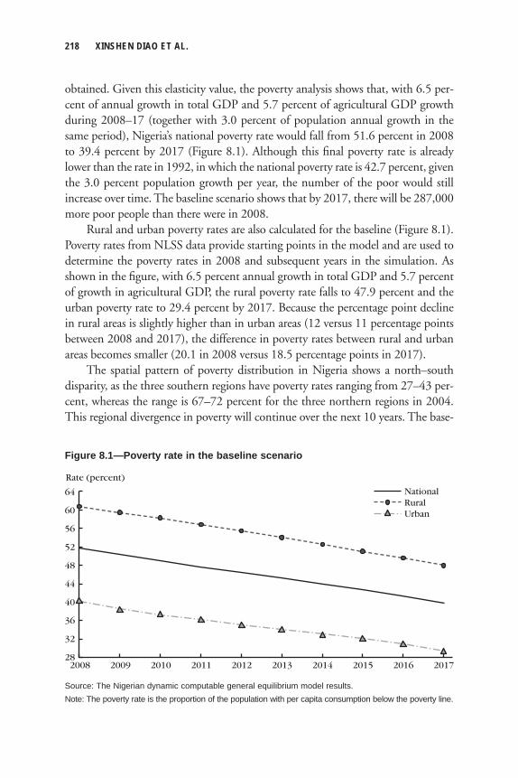
218 XINSHEN DIAO ET AL.
obtained. Given this elasticity value, the poverty analysis shows that, with 6.5 per-cent of annual growth in total GDP and 5.7 percent of agricultural GDP growth during 2008–17 (together with 3.0 percent of population annual growth in the same period), Nigeria’s national poverty rate would fall from 51.6 percent in 2008 to 39.4 percent by 2017 (Figure 8.1). Although this fi nal poverty rate is already lower than the rate in 1992, in which the national poverty rate is 42.7 percent, given the 3.0 percent population growth per year, the number of the poor would still increase over time. The baseline scenario shows that by 2017, there will be 287,000 more poor people than there were in 2008.
Rural and urban poverty rates are also calculated for the baseline (Figure 8.1). Poverty rates from NLSS data provide starting points in the model and are used to determine the poverty rates in 2008 and subsequent years in the simulation. As shown in the fi gure, with 6.5 percent annual growth in total GDP and 5.7 percent of growth in agricultural GDP, the rural poverty rate falls to 47.9 percent and the urban poverty rate to 29.4 percent by 2017. Because the percentage point decline in rural areas is slightly higher than in urban areas (12 versus 11 percentage points between 2008 and 2017), the difference in poverty rates between rural and urban areas becomes smaller (20.1 in 2008 versus 18.5 percentage points in 2017).
The spatial pattern of poverty distribution in Nigeria shows a north–south disparity, as the three southern regions have poverty rates ranging from 27–43 per-cent, whereas the range is 67–72 percent for the three northern regions in 2004. This regional divergence in poverty will continue over the next 10 years. The base-
Rate (percent)
64
28
60
56
52
48
44
36
32
40
2017201620152014201320122011201020092008
NationalRuralUrban
Figure 8.1—Poverty rate in the baseline scenario
Source: The Nigerian dynamic computable general equilibrium model results.Note: The poverty rate is the proportion of the population with per capita consumption below the poverty line.
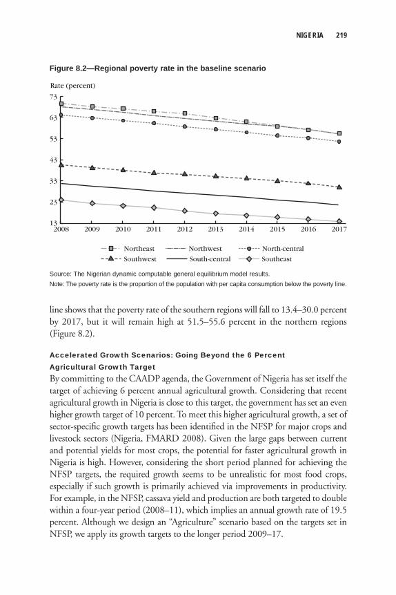
NIGERIA 219
line shows that the poverty rate of the southern regions will fall to 13.4–30.0 percent by 2017, but it will remain high at 51.5–55.6 percent in the northern regions (Figure 8.2).
Accelerated Growth Scenarios: Going Beyond the 6 Percent Agricultural Growth TargetBy committing to the CAADP agenda, the Government of Nigeria has set itself the target of achieving 6 percent annual agricultural growth. Considering that recent agricultural growth in Nigeria is close to this target, the government has set an even higher growth target of 10 percent. To meet this higher agricultural growth, a set of sector-specifi c growth targets has been identifi ed in the NFSP for major crops and livestock sectors (Nigeria, FMARD 2008). Given the large gaps between current and potential yields for most crops, the potential for faster agricultural growth in Nigeria is high. However, considering the short period planned for achieving the NFSP targets, the required growth seems to be unrealistic for most food crops, especially if such growth is primarily achieved via improvements in productivity. For example, in the NFSP, cassava yield and production are both targeted to double within a four-year period (2008–11), which implies an annual growth rate of 19.5 percent. Although we design an “Agriculture” scenario based on the targets set in NFSP, we apply its growth targets to the longer period 2009–17.
Rate (percent)
73
13
63
53
33
23
43
2017201620152014201320122011201020092008
South-central
Northwest North-central
Southwest
Northeast
Southeast
Figure 8.2—Regional poverty rate in the baseline scenario
Source: The Nigerian dynamic computable general equilibrium model results.Note: The poverty rate is the proportion of the population with per capita consumption below the poverty line.
220 XINSHEN DIAO ET AL.
For the 29 crops in the model, there are only 10 crops for which production targets are available in NFSP. There are also targets for fi ve livestock products and the fi shery sector. To model accelerated growth, additional land expansion is assumed for some crops (rice, wheat, cocoa, sugar, and oil palm). For the other crops, live-stock, and fi shery, additional growth is assumed to come via productivity improve-ments only (yield increases in the case of crops). Although production targets are not available for many other crops included in the model, and given that many of them are large agricultural subsectors (for example, maize, sorghum, yams, pulses, and oilseeds), additional productivity growth is also assumed for these crops in the Agriculture scenario. However, changes in land and labor supply are not targeted at the subsector level, because they are endogenous to the model. Table 8.3 describes the current and targeted productivity growth rates for different subsectors in the DCGE model.
Results from the Agriculture scenario show that if the targets for individual crops and agricultural subsectors are achieved over the next nine years, then agricul-tural GDP will grow at 9.5 percent annually. This rate is more than four percentage points higher than the baseline (see Table 8.2). Through economywide linkages, additional growth also occurs in the nonagricultural sectors that have close link-ages with the agricultural sector. As shown in Table 8.1, accelerated agricultural growth is mainly driven by productivity. TFP in the agricultural sector grows at 5.6 percent annually in this scenario instead of 2.3 percent in the baseline. The contri-bution of TFP to agricultural GDP growth also rises, which attracts more capital into the agricultural sector (capital demand in the agricultural sector grows at 7.1 percent annually in this scenario compared to 6.7 percent in the baseline). However, less labor is employed in agriculture (the growth rate falls from 2.2 to 2.1 percent). Productivity-led agricultural growth also benefi ts the nonagricultural sectors. TFP growth in the nonagricultural sector rises to 3.0 percent per year, from 2.5 percent in the baseline. Capital accumulation rates also rise, which allows capital employ-ment in the nonagricultural sector to grow more rapidly than in the baseline.
Sector-level growth is further shown in Table 8.2. Overall, the Agriculture scenario results in an increase in total GDP’s annual growth rate from 6.5 to 8.0 percent. More than 75 percent of additional GDP growth is a direct outcome of accelerated agricultural growth; the other 25 percent comes from an increase in nonagricultural growth via linkages effects.
Subsector Contributions to Agricultural GrowthTable 8.4 reports the contribution of each agricultural subsector in reaching the 10 percent agricultural GDP growth goal (see the last column in the table). The table shows that accelerated growth in cereal crop production, particularly in rice, con-tributes the most to the overall agricultural growth in the Agriculture scenario.
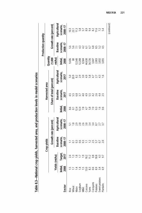
NIGERIA 221
Tabl
e 8.3—
Natio
nal c
rop
yield
s, ha
rves
ted
area
, and
pro
duct
ion
levels
in m
odel
scen
ario
s
Pr
oduc
tion
quan
tity
Grow
th ra
te (p
erce
nt)
Shar
e of t
otal
(per
cent
)
Grow
th ra
te (p
erce
nt)
Ba
selin
e Ag
ricul
tura
l
Base
line
Agric
ultu
ral
Ba
selin
e Ag
ricul
tura
l
Initi
al,
Targ
et,
scen
ario
, sc
enar
io,
Initi
al,
scen
ario
, sc
enar
io,
Initi
al,
scen
ario
, sc
enar
io,
Sect
or
2008
20
17
2008
–17
2008
–17
2008
20
17
2017
20
08
2008
–17
2008
–17
Rice
1.5
2.4
1.1
5.1
8.6
4.5
5.0
9,4
36
5.6
10.3
Whe
at 1.1
1.3
0.1
1.8
0.1
5.5
20
.9 80
5.6
23
.1Ma
ize
1.4
1.8
0.3
2.9
12.4
6.8
8.2
12,54
0 7.1
11
.3So
rghu
m 1.4
1.7
0.6
2.8
12
.4 3.7
2.9
12
,208
4.3
5.8Mi
llet
1.5
1.9
0.3
2.6
7.8
4.0
3.0
8,584
4.2
5.7
Cass
ava
13.0
18.2
1.1
3.8
4.7
4.9
4.9
44,63
0 6.1
8.9
Yams
8.3
11
.2 1.2
3.4
5.8
5.5
5.8
34
,726
6.7
9.4Co
coya
ms
0.6
0.8
2.5
3.4
7.0
4.2
4.7
3,047
6.8
8.2
Potat
oes
8.9
18.8
5.7
8.7
0.3
2.6
2.7
2,003
8.5
11
.6Sw
eet p
otatoe
s 3.4
4.3
0.7
2.7
1.6
4.4
4.3
3,8
32
5.2
7.2Pl
antai
ns
6.9
9.7
2.0
3.7
0.6
2.5
1.6
3,055
4.5
5.4
(cont
inued
)
Cr
op yi
elds
Harv
este
d ar
ea
Yield
s (m
t/ha)
Quan
tity
(1,00
0 m
t/ha)
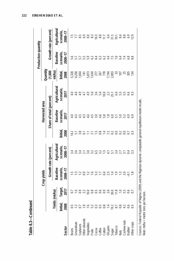
222 XINSHEN DIAO ET AL.
Tabl
e 8.3—
Cont
inue
d
Pr
oduc
tion
quan
tity
Grow
th ra
te (p
erce
nt)
Shar
e of t
otal
(per
cent
)
Grow
th ra
te (p
erce
nt)
Ba
selin
e Ag
ricul
tura
l
Base
line
Agric
ultu
ral
Ba
selin
e Ag
ricul
tura
l
Initi
al,
Targ
et,
scen
ario
, sc
enar
io,
Initi
al,
scen
ario
, sc
enar
io,
Initi
al,
scen
ario
, sc
enar
io,
Sect
or
2008
20
17
2008
–17
2008
–17
2008
20
17
2017
20
08
2008
–17
2008
–17
Bean
s 0.5
0.7
1.5
3.4
14
.2 4.0
4.0
5,3
28
5.6
7.5Gr
ound
nuts
1.2
1.6
1.3
3.6
5.1
4.3
4.0
4,258
5.7
7.7
Soyb
eans
0.7
0.9
1.2
3.4
3.8
4.5
4.9
1,8
34
5.7
8.5Ot
her o
ilsee
ds
1.8
2.2
0.9
2.1
0.1
4.3
4.7
141
5.3
6.9Ve
getab
les
7.6
10.0
1.2
3.0
1.1
4.6
4.9
5,873
5.9
8.0
Fruit
s 5.2
6.8
1.6
3.2
2.1
4.5
5.0
7,6
34
6.2
8.3Co
coa
0.3
0.5
5.3
6.5
1.5
3.0
3.6
277
8.4
10.3
Coffe
e 0.5
0.6
1.7
3.2
0.8
4.6
5.4
26
7 6.3
8.8
Cotto
n 0.8
0.9
0.4
1.5
1.4
5.8
10
.0 77
8 6.2
11
.7Oi
l palm
1.4
2.0
2.5
4.1
7.2
1.8
2.2
7,1
94
4.4
6.4Su
gar
19.2
30.0
1.4
5.1
0.2
6.0
25.1
2,893
7.5
31
.5To
bacc
o 8.7
11
.8 1.9
3.4
0.0
5.1
6.4
33
7.0
10
.1Nu
ts 0.8
1.0
1.3
2.7
0.2
5.0
5.5
10
7 6.4
8.4
Cash
ew nu
ts 4.2
5.5
2.0
3.1
0.0
5.2
5.5
25
7.4
8.8
Rubb
er
0.6
0.6
–0.1
0.4
0.7
6.9
6.6
305
6.8
6.9Ot
her c
rops
0.5
0.7
1.8
3.3
0.3
6.9
9.3
13
4 8.8
12
.9
Sour
ces:
Fede
ral R
epub
lic of
Nige
ria (2
009)
and t
he N
igeria
n dyn
amic
comp
utable
gene
ral e
quilib
rium
mode
l resu
lts.
Note:
mt/h
a = m
etric
tons p
er he
ctare
.
Cr
op yi
elds
Harv
este
d ar
ea
Yield
s (m
t/ha)
Quan
tity
(1,00
0 m
t/ha)
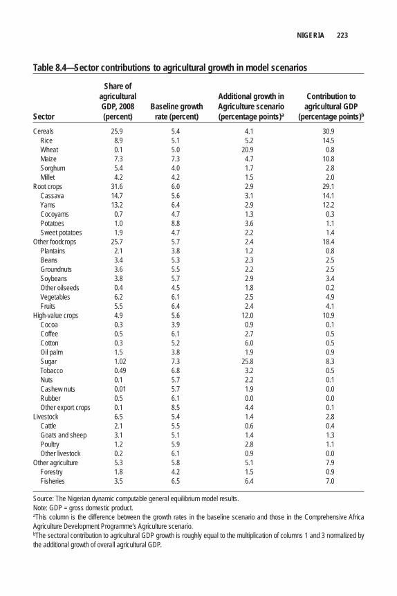
NIGERIA 223
Table 8.4—Sector contributions to agricultural growth in model scenarios
Share of agricultural Additional growth in Contribution to GDP, 2008 Baseline growth Agriculture scenario agricultural GDPSector (percent) rate (percent) (percentage points)a (percentage points)b
Cereals 25.9 5.4 4.1 30.9 Rice 8.9 5.1 5.2 14.5 Wheat 0.1 5.0 20.9 0.8 Maize 7.3 7.3 4.7 10.8 Sorghum 5.4 4.0 1.7 2.8 Millet 4.2 4.2 1.5 2.0Root crops 31.6 6.0 2.9 29.1 Cassava 14.7 5.6 3.1 14.1 Yams 13.2 6.4 2.9 12.2 Cocoyams 0.7 4.7 1.3 0.3 Potatoes 1.0 8.8 3.6 1.1 Sweet potatoes 1.9 4.7 2.2 1.4Other foodcrops 25.7 5.7 2.4 18.4 Plantains 2.1 3.8 1.2 0.8 Beans 3.4 5.3 2.3 2.5 Groundnuts 3.6 5.5 2.2 2.5 Soybeans 3.8 5.7 2.9 3.4 Other oilseeds 0.4 4.5 1.8 0.2 Vegetables 6.2 6.1 2.5 4.9 Fruits 5.5 6.4 2.4 4.1High-value crops 4.9 5.6 12.0 10.9 Cocoa 0.3 3.9 0.9 0.1 Coffee 0.5 6.1 2.7 0.5 Cotton 0.3 5.2 6.0 0.5 Oil palm 1.5 3.8 1.9 0.9 Sugar 1.02 7.3 25.8 8.3 Tobacco 0.49 6.8 3.2 0.5 Nuts 0.1 5.7 2.2 0.1 Cashew nuts 0.01 5.7 1.9 0.0 Rubber 0.5 6.1 0.0 0.0 Other export crops 0.1 8.5 4.4 0.1Livestock 6.5 5.4 1.4 2.8 Cattle 2.1 5.5 0.6 0.4 Goats and sheep 3.1 5.1 1.4 1.3 Poultry 1.2 5.9 2.8 1.1 Other livestock 0.2 6.1 0.9 0.0Other agriculture 5.3 5.8 5.1 7.9 Forestry 1.8 4.2 1.5 0.9 Fisheries 3.5 6.5 6.4 7.0
Source: The Nigerian dynamic computable general equilibrium model results.Note: GDP = gross domestic product. aThis column is the difference between the growth rates in the baseline scenario and those in the Comprehensive Africa Agriculture Development Programme’s Agriculture scenario. bThe sectoral contribution to agricultural GDP growth is roughly equal to the multiplication of columns 1 and 3 normalized by the additional growth of overall agricultural GDP.
224 XINSHEN DIAO ET AL.
Cereal crop production as a whole contributes 30.9 percent to accelerated agricul-tural growth, and rice contributes 14.5 percent. These large contributions are to be expected, because cereal crops constitute the second largest agricultural subsector after root crops (accounting for 25.9 percent of initial agricultural GDP in 2006). They also have the highest growth targets in NFSP. For example, targeted rice pro-duction by 2017 requires almost 10 percent annual growth during 2009–17. Among the fi ve cereal crops, wheat has the highest growth rate in the Agriculture scenario because of the self-suffi ciency target in NFSP. To meet such an ambitious target, wheat must grow at 26 percent per year over the next nine years. However, because this sector is only a small share of total agriculture, even such extremely rapid growth contributes little to overall agricultural growth (0.8 percent in total).
After cereals, root crops are the second most important group contributing to agricultural growth, even though this group is the largest agricultural subsector, currently composing 31.6 percent of agricultural GDP. Among the fi ve root crops, it is only cassava for which a national target has been set in NFSP. We assume modest additional growth in the other four roots and tubers. However, because their growth is lower than for most cereal crops, root crops as a whole only account for 2.9 per-cent of additional growth in the Agriculture scenario and 29.1 percent of agricul-tural growth. Given its large share of agricultural GDP, cassava is still the second most important contributor to growth, accounting for 14.1 percent of accelerated agricultural growth. Yams rank third with a contribution of 12.2 percent.
The diversity of diets and food production in Nigeria means that there are many foodcrops that are important for food security and poverty reduction. We group these into “other foodcrops,” which in total accounts for 25.7 percent of agricultural GDP—the third largest subsector after roots and cereals. Consistent with its large size, this group of crops is the third most important contributor to growth, generating 18.4 percent of additional agricultural growth.
There are 10 high-value crops in the model, namely, cashew nuts, cocoa, coffee, cotton, nuts, oil palm, rubber, sugar, tobacco, and other export crops. Most of these are export-oriented and are either currently important export crops or were in the past. The 10 crops together account for 4.9 percent of agricultural GDP and con-stitute the smallest agricultural subsector in the economy. High growth is assumed for these crops, driven by the extremely high growth in sugar to meet the target set in NFSP. As a group, the additional annual growth rate in the Agriculture scenario is 12 percent, rising from the baseline of 5.6 percent to 17.6 percent. However, their small share of the agricultural economy means that these crops’ contribution to accelerated agricultural growth is less important than foodcrops’ contribution. What contribution there is due primarily to sugar production.
Primary livestock production currently accounts for 6.5 percent of agricultural GDP. Targets for most livestock products are available in NFSP. Consistent with these targets, a rapid growth is assumed in the Agriculture scenario for poultry
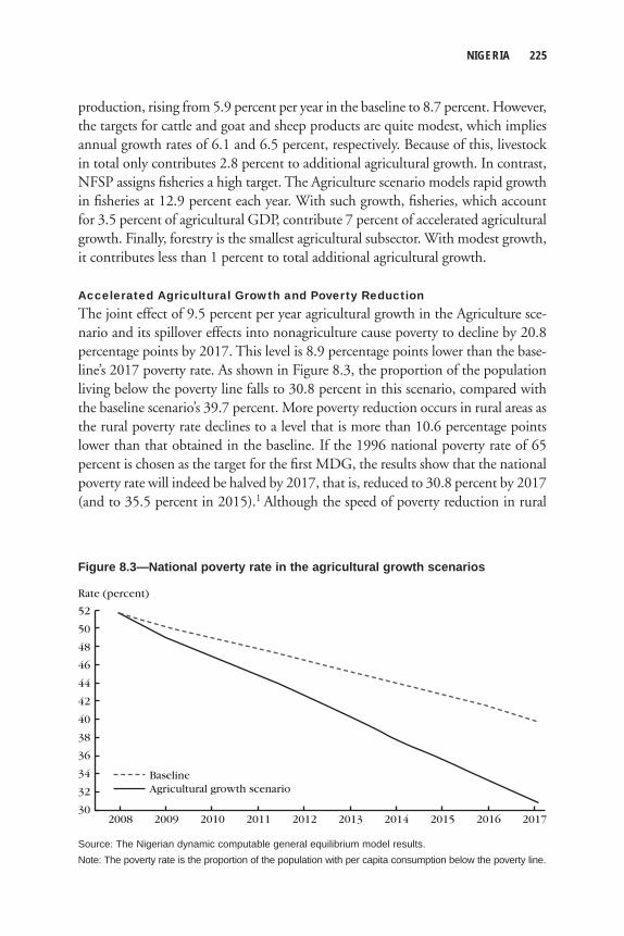
NIGERIA 225
production, rising from 5.9 percent per year in the baseline to 8.7 percent. However, the targets for cattle and goat and sheep products are quite modest, which implies annual growth rates of 6.1 and 6.5 percent, respectively. Because of this, livestock in total only contributes 2.8 percent to additional agricultural growth. In contrast, NFSP assigns fi sheries a high target. The Agriculture scenario models rapid growth in fi sheries at 12.9 percent each year. With such growth, fi sheries, which account for 3.5 percent of agricultural GDP, contribute 7 percent of accelerated agricultural growth. Finally, forestry is the smallest agricultural subsector. With modest growth, it contributes less than 1 percent to total additional agricultural growth.
Accelerated Agricultural Growth and Poverty ReductionThe joint effect of 9.5 percent per year agricultural growth in the Agriculture sce-nario and its spillover effects into nonagriculture cause poverty to decline by 20.8 percentage points by 2017. This level is 8.9 percentage points lower than the base-line’s 2017 poverty rate. As shown in Figure 8.3, the proportion of the population living below the poverty line falls to 30.8 percent in this scenario, compared with the baseline scenario’s 39.7 percent. More poverty reduction occurs in rural areas as the rural poverty rate declines to a level that is more than 10.6 percentage points lower than that obtained in the baseline. If the 1996 national poverty rate of 65 percent is chosen as the target for the fi rst MDG, the results show that the national poverty rate will indeed be halved by 2017, that is, reduced to 30.8 percent by 2017 (and to 35.5 percent in 2015).1 Although the speed of poverty reduction in rural
Rate (percent)
52
Baseline
30
46
48
50
44
42
40
38
34
32
36
Agricultural growth scenario
2017201620152014201320122011201020092008
Figure 8.3—National poverty rate in the agricultural growth scenarios
Source: The Nigerian dynamic computable general equilibrium model results.Note: The poverty rate is the proportion of the population with per capita consumption below the poverty line.
226 XINSHEN DIAO ET AL.
areas is faster than in urban ones, the poverty rate in the Agriculture scenario will remain high at 37.3 percent and will not achieve the fi rst MDG in rural areas. In contrast, the urban poverty rate will fall to 22.6 percent by 2017 (and 26.2 percent in 2015), thus declining more than 50 percent from its 1996 value. Although faster agricultural growth reduces the divide between rural and urban areas, the country still faces the challenge of how to accelerate poverty reduction in rural areas.
Achieving the targets in the Agriculture scenario will lift an additional 16.5 million people above the poverty line by 2017, thereby reversing the current rising trend in the number poor people. Even with 3.0 percent of annual population growth, the absolute number of the poor will still fall to 59.7 million by 2017 (from the current 77 million, and 78.7 million in the baseline’s 2017). Food security would also improve, with an additional 140 kilograms of cereals and 300 kilograms of root products available per capita by 2017 compared to current per capita avail-ability. Furthermore, although Nigeria will continue to import some cereal prod-ucts, such as wheat and rice, the ratio of imports in domestic consumption will be substantially lower than that in the baseline scenario.
Faster agricultural growth benefi ts a majority of households. However, not all households will benefi t equally from achieving the crop and livestock growth targets in the Agriculture scenario. For this reason, we also investigate the poverty impact at the zonal level for the six regions. Results are reported in Table 8.5. The fi rst two columns of the table report poverty rates in 1996 and 2004. The third and fourth columns report the poverty rates for 2017 from the baseline and Agriculture sce-narios. To make the comparison across regions easy to read, we also report the re-duction in poverty rates as both percentage points and percent changes, both relative to 1996 and the baseline scenario’s 2017. These numbers are found in the fi nal four columns of the table. Finally, the national poverty rates are included for the country as a whole and for the rural and urban areas separately in the fi rst part of the table (rows 1–3).
As seen in Table 8.5, there exists signifi cant spatial disparity in Nigeria’s poverty distribution. NLSS 2003/04 indicates that the three northern regions have higher poverty rates than do the southern regions, although this disparity was less signifi -cant in 1996 (see the second and third columns in the table). The regional differ-ences in poverty do not change in the baseline and Agriculture scenarios. For example, the highest regional poverty rate in 2004 was in the Northeast (72.2 percent). This situation will continue until 2017 in both scenarios. The spatial poverty gap, mea-sured by the difference between the highest regional poverty rate in the Northeast and the lowest poverty rate that is in the Southeast, was 45.5 percentage points in 2004 (the most recent year for which the poverty information is available). By 2017, this gap is smaller in both scenarios but will still be 43.8–35.2 percentage points. Measured by the percentage change from the level of poverty in 1996, it is reason-
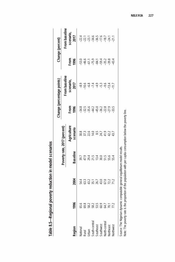
NIGERIA 227
Tabl
e 8.5—
Regi
onal
pove
rty re
duct
ion
in m
odel
scen
ario
s
Chan
ge (p
erce
ntag
e poi
nts)
Ch
ange
(per
cent
)
From
bas
eline
From
bas
eline
Agric
ultu
re
From
sc
enar
io,
From
sc
enar
io,
Regi
on
1996
20
04
Base
line
scen
ario
19
96
2017
19
96
2017
Natio
nal
65.6
54.4
39.7
30.8
–34.8
–8
.9 –5
3.0
–22.4
Rura
l 69
.8 63
.3 47
.9 37
.3 –3
2.5
–10.6
–4
6.6
–22.1
Urba
n 58
.2 43
.2 29
.4 22
.6 –3
5.6
–6.8
–61.1
–2
3.1So
uth-ce
ntral
58.2
35.1
21.5
14.0
–44.2
–7
.4 –7
5.9
–34.6
South
east
53.5
26.7
13.4
8.5
–45.0
–4
.9 –8
4.1
–36.5
South
west
60.9
43.0
30.0
24.7
–36.2
–5
.3 –5
9.4
–17.6
North
-centr
al 64
.7 67
.0 51
.5 41
.9 –2
2.8
–9.6
–35.2
–1
8.7No
rthea
st 70
.1 72
.2 55
.6 42
.2 –2
7.9
–13.4
–3
9.8
–24.1
North
west
77.2
71.2
55.4
43.7
–33.5
–1
1.7
–43.4
–2
1.1
Sour
ce: T
he N
igeria
n dyn
amic
comp
utable
gene
ral e
quilib
rium
mode
l resu
lts.
Note:
The
pove
rty ra
te is
the pr
opor
tion o
f the p
opula
tion w
ith pe
r cap
ita co
nsum
ption
below
the p
over
ty lin
e.
Pove
rty ra
te, 2
017 (
perc
ent)
228 XINSHEN DIAO ET AL.
able to expect that accelerated high agricultural growth will allow the southern regions to achieve the fi rst MDG of halving the 1996 poverty rate by 2015. However, this will not be the case for the three northern regions.
Because there are no growth targets at the state or regional level, we have assumed a uniform target for each crop or livestock subsector across the six regions. Initial conditions and growth potentials are very different between the north and south. Analysis of NLSS 2003/04 and Core Welfare Indicator Survey (Nigeria, NBS 2007b) data shows that initial production conditions, such as access to fertilizer, are far worse in the north than in the south. Without special attention paid to the northern regions in terms of public investment, modern input access, and other input and output market development, the growth opportunities may be further biased toward the south. Unless this issue is given priority by the government, pov-erty reduction goals will be more diffi cult to achieve in the north.
Growth Multipliers and Subsector Contributions to Poverty ReductionWe now design a series of scenarios in which growth in some major crops or group of crops or livestock products are individually simulated, while assuming that pro-ductivity in other crops and subsectors remains at baseline levels. Although produc-tivity growth in a subsector can be assumed exogenously, it does not imply that there is no growth impact on any other subsectors. Other sectors’ growth is affected through linkage effects captured in the DCGE model. These effects include com-petition (and reallocation) over factors and inputs across subsectors, changes in rela-tive prices, and changes in domestic demand and international trade. Because of these complex linkages, growth in subsectors other than the targeted subsector can be affected positively or negatively. For example, if increased maize supply can easily fi nd demand (domestically or internationally) and the maize price does not fall signifi cantly, then maize production will compete with other crops for additional resources (land or labor) and intermediate inputs (for example, fertilizer). Thus, growth in some crops, such as sorghum or millet, could be negatively affected. In contrast, if there are demand constraints stemming from low income elasticity of demand or a lack of export/import substitution opportunities, then domestic maize prices will fall. In this case, even if maize yield rises, maize output could increase by less than the growth in yields. Resources will then be released from maize produc-tion, and production of other crops could increase. These linkage effects imply that the realization of growth targets is jointly determined by supply and demand in the market. Therefore, policies affecting demand (including market development and access) are equally important for accelerating agricultural growth.
Understanding the magnitude of poverty reduction led by a specifi c sector’s growth is important when designing pro-poor growth strategies. We analyze these linkages by calculating poverty–growth elasticities and growth multipliers. The latter
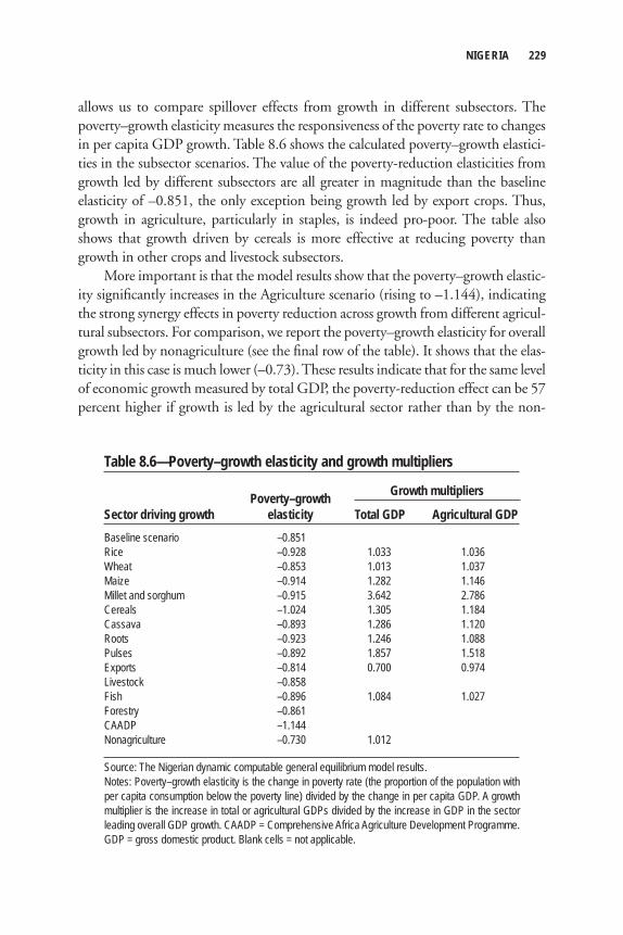
NIGERIA 229
allows us to compare spillover effects from growth in different subsectors. The poverty–growth elasticity measures the responsiveness of the poverty rate to changes in per capita GDP growth. Table 8.6 shows the calculated poverty–growth elastici-ties in the subsector scenarios. The value of the poverty-reduction elasticities from growth led by different subsectors are all greater in magnitude than the baseline elasticity of –0.851, the only exception being growth led by export crops. Thus, growth in agriculture, particularly in staples, is indeed pro-poor. The table also shows that growth driven by cereals is more effective at reducing poverty than growth in other crops and livestock subsectors.
More important is that the model results show that the poverty–growth elastic-ity signifi cantly increases in the Agriculture scenario (rising to –1.144), indicating the strong synergy effects in poverty reduction across growth from different agricul-tural subsectors. For comparison, we report the poverty–growth elasticity for overall growth led by nonagriculture (see the fi nal row of the table). It shows that the elas-ticity in this case is much lower (–0.73). These results indicate that for the same level of economic growth measured by total GDP, the poverty-reduction effect can be 57 percent higher if growth is led by the agricultural sector rather than by the non-
Table 8.6—Poverty–growth elasticity and growth multipliers
Poverty–growthSector driving growth elasticity Total GDP Agricultural GDPBaseline scenario –0.851 Rice –0.928 1.033 1.036Wheat –0.853 1.013 1.037Maize –0.914 1.282 1.146Millet and sorghum –0.915 3.642 2.786Cereals –1.024 1.305 1.184Cassava –0.893 1.286 1.120Roots –0.923 1.246 1.088Pulses –0.892 1.857 1.518Exports –0.814 0.700 0.974Livestock –0.858 Fish –0.896 1.084 1.027Forestry –0.861 CAADP –1.144 Nonagriculture –0.730 1.012
Source: The Nigerian dynamic computable general equilibrium model results.Notes: Poverty–growth elasticity is the change in poverty rate (the proportion of the population with per capita consumption below the poverty line) divided by the change in per capita GDP. A growth multiplier is the increase in total or agricultural GDPs divided by the increase in GDP in the sector leading overall GDP growth. CAADP = Comprehensive Africa Agriculture Development Programme. GDP = gross domestic product. Blank cells = not applicable.
Growth multipliers
230 XINSHEN DIAO ET AL.
agricultural sector. These results have strong implication for Nigeria’s development strategy and for the allocation of public funds. This issue is discussed later in this chapter.
Growth multipliers are another important indicator for measuring the differ-ential contribution of agricultural growth at the subsector level to economywide growth. We omit the multiplier results for the cases in which growth is led by live-stock and forestry, because we also exogenously assume additional productivity growth in their relevant processing sectors in these scenarios. For example, in the livestock-led growth scenario, additional productivity growth in meat and milk processing is considered; in the forestry-led growth scenario the wood-processing growth is considered. Because additional productivity growth from these non-agricultural subsectors is assumed in these scenarios, it makes them diffi cult to com-pare with growth led by the crop subsectors and fi sheries.
Among the three groups of crops, the highest growth multiplier is for pulses. This is true for the multipliers measured against both total and agricultural GDP. The results indicate that a unit increase in pulses production (real value-added) causes a 1.857-unit increase in total GDP or a 1.518-unit increase in agricultural GDP (in real terms). This high multiplier indicates strong linkages between pulse production and other economic activities. Similarly, cassava has a high growth multi-plier among root crops.
At the individual crop level, millet and sorghum have the strongest multiplier effects. Economic linkages on the supply side come from (1) increased demand in intermediate inputs (that is, backward linkages); (2) provision of more low-cost inputs to other agricultural or food processing production (that is, forward link-ages); and (3) release of resources (land and labor) to be used by other crops (that is, factor mobility linkages). Demand-side linkages are also strong and arise through increased demand for other agricultural and nonagricultural commodities as the result of increased farmer incomes from the additional growth of production in some agricultural subsectors. However, in the case of millet and sorghum, for which the highest growth multiplier is obtained in the simulation, the main reason is the effects of factor mobility linkages. Millet and sorghum are income-inelastic com-modities: at higher income levels, households spend less income to consume addi-tional millet and sorghum and prefer to allocate more income into consumption of other foods, such as rice, wheat, or livestock products. Growth in millet and sor-ghum supply from increased productivity is not necessarily the same as growth in the two crops’ yields, which implies less land and labor are needed to produce these two crops when their yields increase. When fewer resources are used to produce millet and sorghum without lowering the supply level of these two crops (that is, when part of the land and labor initially used for millet and sorghum production can be released and reallocated into production of other crops, such as rice, maize,
NIGERIA 231
and wheat), the strong growth multiplier occurs. Thus, in the case of millet and sorghum, the model result seems to indicate that resources (primarily land) allocated to the production of these two crops are excessive when these two crops’ productivity is low. Thus, when millet and sorghum become more productive, many other agri-cultural subsectors and the economy as a whole benefi t through the multiplier effect of the two crops with the rest of economy.
However, the value of the growth multiplier measured by gains in GDP in the case of growth led by export crop is smaller than one (see Table 8.6). When the growth multiplier is less than one, it indicates that, at the given level of resources, growth in some other sectors is negatively affected by the growth in the targeted subsectors (export crops in this case). The main reason is that domestic prices for export-oriented commodities are mainly determined by the international markets. With such price advantages, export-oriented sectors will compete with other sectors for resources (land, labor, capital, and other inputs). At the given resource level, competition affects the factor prices, which in turn makes it diffi cult for many other sectors to increase production. Of course, with fewer resources allocated, production in the other sectors falls. This result has important policy implication. Although developing export-oriented agricultural production is often high on the agenda of the government, growth in such production will have weak linkages with the domes-tic economy if there are no additional resources (land and labor) available in the country, or if export-oriented production cannot create domestic demand for such products (either through development of agroprocessing or through consumer demand). Focusing on export-oriented crops may also have negative effects on growth outside export-oriented production, which results in smaller economywide gains from such a strategy.
Price Effects from Accelerated Agricultural GrowthEven if productivity-led agricultural growth benefi ts a majority of households in both rural and urban areas, negative price effect from such growth can hurt some farmers. For those farmers who are unable to adopt the high-yield technology and still use traditional farming technology, lowered output prices caused by increased production from other, more productive, farmers implies that their revenues from producing the same amount of products fall. In contrast, for those farmers who have adopted the high-yield technology but are facing increased input prices (for exam-ple, higher fertilizer price), lowered output prices together with increased input prices might make them less profi table despite using modern technology. Thus, it is necessary to assess the possible price effect from accelerated agricultural growth in the Agriculture scenario.
Figure 8.4 shows the price trends for selected agricultural products in the Agriculture scenario. In Figure 8.4 prices for individual agricultural commodities
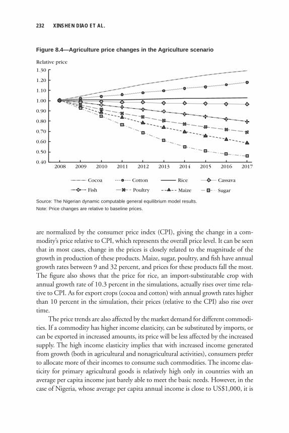
232 XINSHEN DIAO ET AL.
are normalized by the consumer price index (CPI), giving the change in a com-modity’s price relative to CPI, which represents the overall price level. It can be seen that in most cases, change in the prices is closely related to the magnitude of the growth in production of these products. Maize, sugar, poultry, and fi sh have annual growth rates between 9 and 32 percent, and prices for these products fall the most. The fi gure also shows that the price for rice, an import-substitutable crop with annual growth rate of 10.3 percent in the simulations, actually rises over time rela-tive to CPI. As for export crops (cocoa and cotton) with annual growth rates higher than 10 percent in the simulation, their prices (relative to the CPI) also rise over time.
The price trends are also affected by the market demand for different commodi-ties. If a commodity has higher income elasticity, can be substituted by imports, or can be exported in increased amounts, its price will be less affected by the increased supply. The high income elasticity implies that with increased income generated from growth (both in agricultural and nonagricultural activities), consumers prefer to allocate more of their incomes to consume such commodities. The income elas-ticity for primary agricultural goods is relatively high only in countries with an average per capita income just barely able to meet the basic needs. However, in the case of Nigeria, whose average per capita annual income is close to US$1,000, it is
Relative price
1.30
0.40
1.20
1.10
0.90
0.80
0.70
0.60
0.50
1.00
2017201620152014201320122011201020092008
RiceCocoa Cotton
Maize Sugar
Cassava
Fish Poultry
Figure 8.4—Agriculture price changes in the Agriculture scenario
Source: The Nigerian dynamic computable general equilibrium model results.Note: Price changes are relative to baseline prices.
NIGERIA 233
unlikely that most primary agricultural products will have high income elasticities. Although the income elasticities for the foods consumed by the poor in rural and urban areas are higher than that for the country as whole, they are unlikely to become the driving force in determining market demand, given the current income distribution in the country.
However, besides import substitution (such as in the case of rice and wheat), there are market opportunities for agriculture by developing agroprocessing indus-tries in the country and by expanding the export market. Nigeria has the largest agroprocessing industry in West Africa. Promising export opportunities for many staple commodities do exist in both regional and global markets. An example is cassava, which accounts for the largest land allocation and highest agricultural value-added of any sector in the country. Cassava chips and fl ours are excellent inputs for both the feed and agroprocessing sectors and are in high demand in international markets as well. For instance, Thailand, which accounts for 10 percent of the world cassava production, exports 80 percent of its cassava products. Currently with around 22 million metric tons of cassava traded mostly as chips and fl our, this country controls 70–80 percent of the world cassava market. In contrast, cassava in Nigeria is mainly for domestic food consumption. It is therefore reasonable to think that with the adoption of high-yield varieties, cost-effective processing technologies, and improved market access conditions, Nigeria could successfully export cassava to the rest of the world. In such a scenario, Nigeria could become one of the domi-nant cassava exporters in the world, and both the growth multiplier and poverty-reduction–growth elasticity of cassava-led growth would further increase.
Another example is the poultry sector. The results of our model show that poultry prices fall signifi cantly when a high growth in poultry is targeted. However, current domestic poultry prices are not competitive, and without border protection in imports, domestic poultry prices would not be as high as they currently are. The model result actually shows that only through improving the poultry sector’s pro-ductivity can the country eventually get rid of its import restriction, so that poultry could become an export commodity to the neighborhood countries in West Africa. Development of a modern poultry industry would provide the country not only with great export opportunities in poultry products but also would create more domestic demand for maize and other crops as poultry feed, which would further enhance the linkage and multiplier effects in the entire economy. The successful experience of Thailand becoming a large poultry exporter since the late 1980s illus-trates such possibilities. The rapid growth in poultry exports has created a big market for maize in the country. Before that, feed demand in Thailand accounted for only a small portion of maize production (3–7 percent), similar to the situation in Nigeria today. With the development of the poultry industry, feed demand in Thailand now accounts for 70–80 percent of maize production (a tenfold increase
234 XINSHEN DIAO ET AL.
over two decades). It is therefore reasonable to believe that development of the poultry sector in Nigeria offers an opportunity for maize production to grow, mak-ing it not only an important staple commodity for human consumption but also an important cash crop for many smallholder farmers. Table 8.7 summarizes the fi ndings of our analysis in this section.
Agricultural Investment AnalysisBased on the DCGE model results, we estimate the required public investments in agriculture for 2009–17 in this section. In Nigeria supporting the agricultural sector is a joint responsibility of the three tiers of governments, federal, state, and local, as mandated by the 1999 constitution. To quantitatively estimate the required agricul-tural spending, the availability of time series data for the three tiers of government expenditure is critical. Unfortunately, we are unable to obtain spending data by different items (for example, spending on research and extension or on fertilizer subsidies) for any tier of government, and local government total spending data are also limited to a few recent years. Thus, we only consider federal and state total spending in the analysis. The methodology introduced in Chapter 2 is used here. It is based on an estimated elasticity relating agricultural TFP to public agricultural spending (a growth –spending elasticity). An agricultural TFP time series was obtained from Nin Pratt and Yu (2008).
The results of our investment analysis show that the growth–spending elasticity for Nigeria is 0.24. Although this elasticity is used in the analysis, to further analyze the sensitivity of required spending with respect to the choice of elasticity (which partially refl ects the effi ciency of spending), we also consider a case in which the elasticity increases to 0.41, which is close to the one obtained for cross-country estimations treating Sub-Saharan Africa as a whole. Agricultural growth is also affected by nonagricultural investment, and hence, the latter is also needed to esti-mate the agricultural growth response to nonagricultural spending. The estimated result is 0.46, rather high compared with the elasticity with respect to the agricul-tural spending. Given that most public good provision, including investment in infrastructure and spending on education and health, is counted as part of non-agricultural spending, the estimation result is not surprising, because such spending defi nitely benefi ts the entire economy, including the rural economy and the agri-cultural sector. However, measured as returns to the amount of spending, non-agricultural spending is not necessarily more effective than agricultural spending in terms of promoting agricultural growth. The size of nonagricultural spending is 20–25 times that of agricultural spending in Nigeria, which implies that a 1 percent increase in nonagricultural spending is equivalent to a 20–25 percent increase in agricultural spending. Thus, the dollar-to-dollar comparison still indicates that
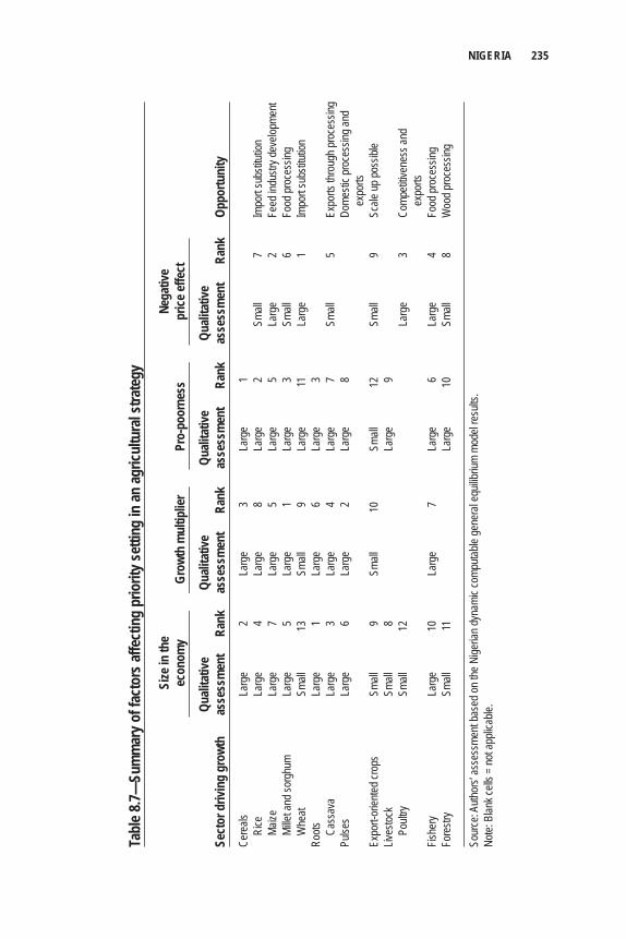
NIGERIA 235
Tabl
e 8.7—
Sum
mar
y of f
acto
rs af
fect
ing
prio
rity s
ettin
g in
an ag
ricul
tura
l stra
tegy
Si
ze in
the
Nega
tive
ec
onom
y Gr
owth
mul
tiplie
r Pr
o-po
orne
ss
price
effe
ct
Qu
alita
tive
Qu
alita
tive
Qu
alita
tive
Qu
alita
tive
Sect
or d
rivin
g gr
owth
as
sess
men
t Ra
nk
asse
ssm
ent
Rank
as
sess
men
t Ra
nk
asse
ssm
ent
Rank
Op
portu
nity
Cere
als
Larg
e 2
Larg
e 3
Larg
e 1
Ri
ce
Larg
e 4
Larg
e 8
Larg
e 2
Small
7
Impo
rt su
bstitu
tion
Ma
ize
Larg
e 7
Larg
e 5
Larg
e 5
Larg
e 2
Feed
indu
stry d
evelo
pmen
t
Mille
t and
sorg
hum
Larg
e 5
Larg
e 1
Larg
e 3
Small
6
Food
proc
essin
g
Whe
at Sm
all
13
Small
9
Larg
e 11
La
rge
1 Im
port
subs
titutio
nRo
ots
Larg
e 1
Larg
e 6
Larg
e 3
Ca
ssav
a La
rge
3 La
rge
4 La
rge
7 Sm
all
5 Ex
ports
thro
ugh p
roce
ssing
Pulse
s La
rge
6 La
rge
2 La
rge
8
Do
mesti
c pro
cess
ing an
d
ex
ports
Expo
rt-or
iented
crop
s Sm
all
9 Sm
all
10
Small
12
Sm
all
9 Sc
ale up
poss
ible
Lives
tock
Small
8
Larg
e 9
Po
ultry
Small
12
La
rge
3 Co
mpeti
tiven
ess a
nd
expo
rtsFis
hery
Larg
e 10
La
rge
7 La
rge
6 La
rge
4 Fo
od pr
oces
sing
Fore
stry
Small
11
La
rge
10
Small
8
Woo
d pro
cess
ing
Sour
ce: A
uthor
s’ as
sess
ment
base
d on t
he N
igeria
n dyn
amic
comp
utable
gene
ral e
quilib
rium
mode
l resu
lts.
Note:
Blan
k cell
s = no
t app
licab
le.
236 XINSHEN DIAO ET AL.
agricultural spending is more effective than nonagricultural spending for agricul-tural productivity growth.
But we are skeptical of using this nonagricultural spending elasticity in the analysis for the following reasons. First, constrained by the data availability, we have to defi ne nonagricultural spending as the difference between total spending and agricultural spending. Thus, part of spending that is classifi ed as nonagricultural may directly target agricultural and rural development (for example, rural road and rural electrifi cation). Second, the quality of data for agricultural spending is rela-tively poor compared with the total spending data, and agricultural spending is a small portion of total spending (less than 4 percent in most years). As a result, the data are likely to produce a biased estimate by not fully distinguishing between the direct and indirect effects of nonagricultural spending. Furthermore, the estimated nonagricultural elasticity is inconsistent with growth in both agricultural and non-agricultural spending if we use it to calibrate the historical data. For these reasons, a calibration method is applied in this study for the nonagricultural elasticity using the historical data for agricultural and nonagricultural spending and growth in agricultural TFP, together with the estimated elasticity for the agricultural spending. The calibrated nonagricultural spending elasticity is 0.14.
We consider four scenarios in assessing the growth in agricultural spending required to support the 5.62 percent agricultural TFP growth rate obtained from the Agriculture scenario of the DCGE model. In the fi rst scenario, the elasticity of agricultural TFP with respect to agriculture spending as our estimation result (0.24) is applied. We assume that the growth rate of nonagricultural spending is the same as that of the current trend (which is the same as in the baseline). Combining this value with an elasticity of 0.14 with respect to the nonagricultural spending, our analysis shows that 23.8 percent of annual growth in agricultural spending is required in 2009–17 to support the target of 9.45 percent agricultural growth (and 5.62 percent agricultural TFP growth). This result is consistent with the estimation of Fan, Yu, and Saurkar (2008), in which 25.1 percent of annual growth is required for agricultural spending to achieve the fi rst MDG in Nigeria. However, when the agricultural spending is assumed to be more effi cient in the second scenario of our analysis (that is, the value of elasticity is increased from 0.24 to 0.41), required agricultural spending only needs to grow at 13.6 percent per year (Table 8.8).
Using the additional growth in agricultural spending and given the growth in the nonagricultural spending, the share of agricultural spending in government total expenditure rises gradually. Currently, agriculture accounts for 4.2 percent of total government expenditure; this share will eventually rise to 14.6 percent by 2015 and 18.6 percent by 2017 using the low elasticity in the fi rst scenario. In the second scenario with a high elasticity (that is, assuming improved spending effi -ciency), the share of agricultural expenditure in total spending will be 7.3 percent
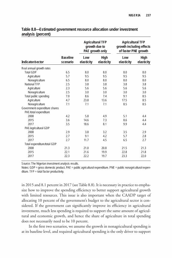
NIGERIA 237
in 2015 and 8.1 percent in 2017 (see Table 8.8). It is necessary in practice to empha-size how to improve the spending effi ciency to better support agricultural growth with limited resources. This issue is also important when the CAADP target of allocating 10 percent of the government’s budget to the agricultural sector is con-sidered. If the government can signifi cantly improve its effi ciency in agricultural investment, much less spending is required to support the same amount of agricul-tural and economic growth, and hence the share of agriculture in total spending does not necessarily need to be 10 percent.
In the fi rst two scenarios, we assume the growth in nonagricultural spending is at its baseline level, and required agricultural spending is the only driver to support
Table 8.8—Estimated government resource allocation under investment analysis (percent)
Agricultural TFP Agricultural TFP growth due to growth including effects PAE growth only of faster PNE growth
Baseline Low High Low HighIndicator/sector scenario elasticity elasticity elasticity elasticityReal annual growth rates Total GDP 6.5 8.0 8.0 8.0 8.0 Agriculture 5.7 9.5 9.5 9.5 9.5 Nonagriculture 6.5 8.0 8.0 8.0 8.0 National TFP 2.5 3.8 3.8 3.8 3.8 Agriculture 2.3 5.6 5.6 5.6 5.6 Nonagriculture 2.5 3.0 3.0 3.0 3.0 Total public spending 7.0 8.6 7.4 9.1 8.5 Agriculture 4.7 23.8 13.6 17.5 8.5 Nonagriculture 7.1 7.1 7.1 8.5 8.5Government expenditure shares PAE/total expenditure 2008 4.2 5.8 4.9 5.1 4.4 2015 3.6 14.6 7.3 8.6 4.4 2017 3.5 18.6 8.1 9.9 4.4 PAE/agricultural GDP 2008 2.9 3.8 3.2 3.5 2.9 2015 2.7 9.1 4.2 5.7 2.8 2017 2.7 11.7 4.5 6.5 2.7 Total expenditure/total GDP 2008 21.3 21.0 20.8 21.5 21.3 2015 22.1 21.6 19.9 22.8 21.8 2017 22.3 22.2 19.7 23.3 22.0
Source: The Nigerian investment analysis results.Notes: GDP = gross domestic product. PAE = public agricultural expenditure. PNE = public nonagricultural expen-diture. TFP = total factor productivity.
238 XINSHEN DIAO ET AL.
accelerated agricultural growth. In other words, we ignore the indirect effect of additional growth in nonagricultural spending on agricultural growth. In the third and fourth scenarios, we consider this factor and re-estimate the required agricul-tural spending using the low and high elasticities, respectively. Increased non-agricultural spending is assumed to be proportional to the nonagricultural sector’s TFP growth, which increases to 2.98 percent per year from 2.47 percent in the baseline. Such growth in the DCGE model is primarily a result of growth link-ages between agriculture and nonagriculture, that is, improvement in the agricul-tural economy benefi ts the nonagricultural sector. Consistent with increased nonagricultural TFP growth, annual growth in nonagricultural spending needs to rise from 7.06 percent in the baseline scenario to 8.52 percent in the accelerated agricultural growth scenario. Additional nonagricultural spending indirectly affects growth in agriculture. Using an elasticity of 0.14 with respect to nonagricultural spending, part of agricultural growth can be indirectly supported by additional government spending on the economy as whole. This lowers required annual growth in the agricultural spending from 23.8 percent to 17.5 percent (in scenario 3) using the low elasticity of agricultural spending (0.24), and from 13.6 percent to 8.5 percent using the high elasticity (0.41, in scenario 4).
Translated into monetary terms, the analysis shows that without taking into account the change in government nonagricultural spending and in the low elastic-ity scenario (scenario 1), the government will need to increase its investments in agriculture from 185 billion Nigerian nairas (NGN185 billion) currently (2008) to NGN1,265 and NGN1,940 billion (in 2006 prices) by 2015 and 2017, respec-tively. In contrast, in the baseline scenario, which follows the current growth trend in government spending, additional agricultural spending will be much lower—only NGN278 and NGN305 billion in 2015 and 2017 (Figure 8.5). When a more optimistic spending effi ciency is assumed in the second scenario (that is, the high elasticity is used), agricultural spending will be NGN583 billion by 2015 and will reach NGN753 billion by 2017, implying that the improvement in investment effi ciency allows the government to save more than NGN4,300 billion in total between 2009 and 2017 or more than NGN400 billion per year on average.
Improvement in agricultural spending effi ciency also reduces the required total government spending. In scenario 1 with the low elasticity, the annual growth in total government expenditure will rise to 8.6 percent (see Table 8.8) and will reach NGN10,452 billion by 2017 (Figure 8.6), in contrast with 7.0 percent annual growth in the baseline and NGN8,817 billion in the baseline’s 2017 prediction. Using the high elasticity in scenario 2, the annual growth in total government spending will be 7.4 percent. As a result, total government expenditure by 2017 stands at NGN9,265 billion, which is only NGN448 billion more than the base-line’s 2017 estimation (see Figure 8.6).
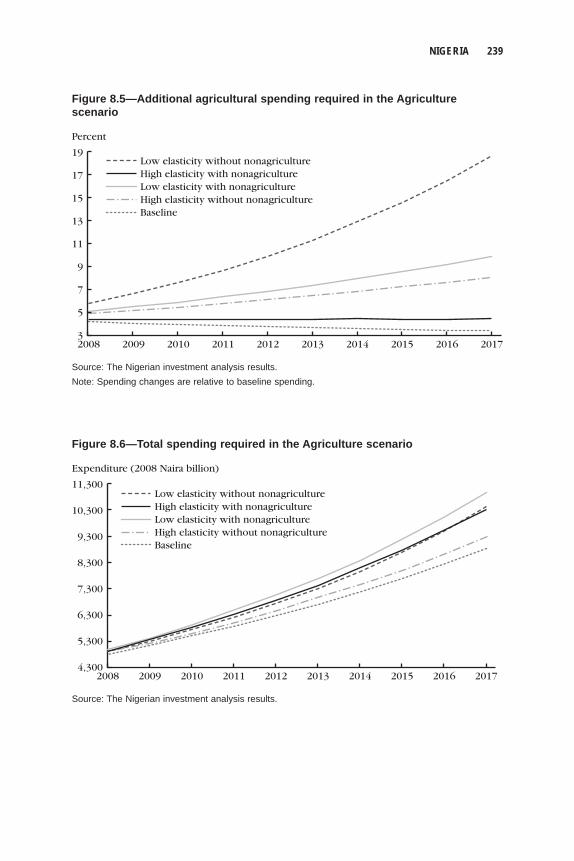
NIGERIA 239
Percent
19
3
13
15
17
11
7
5
9
2017201620152014201320122011201020092008
High elasticity with nonagriculture
High elasticity without nonagricultureLow elasticity with nonagriculture
Baseline
Low elasticity without nonagriculture
Expenditure (2008 Naira billion)
11,300
10,300
9,300
8,300
7,300
6,300
5,300
4,3002017201620152014201320122011201020092008
High elasticity with nonagriculture
High elasticity without nonagricultureLow elasticity with nonagriculture
Baseline
Low elasticity without nonagriculture
Figure 8.5—Additional agricultural spending required in the Agriculture scenario
Source: The Nigerian investment analysis results.Note: Spending changes are relative to baseline spending.
Figure 8.6—Total spending required in the Agriculture scenario
Source: The Nigerian investment analysis results.
240 XINSHEN DIAO ET AL.
In the third and fourth scenarios when additional growth in nonagricultural spending and its indirect effect on agricultural growth are taken into consideration, a relatively slow growth in the required agricultural spending implies a reduced level of such spending over time. Using the low elasticity (scenario 3), the value of agri-cultural spending will reach NGN788 billion and NGN1,087 billion by 2015 and 2017, respectively, whereas the high elasticity in scenario 4, it will be NGN356 billion and NGN455 billion by 2015 and 2017, respectively. However, as additional spending on the nonagricultural sector is taken into account, total government spending will not decline from that in the previous two scenarios. In fact, with either low or high effi ciency in agricultural spending, the total government spending rises over time (see Figure 8.6). That is to say, because nonagriculture accounts for a much larger share of total spending than does agriculture, even with very rapid growth in agricultural spending, the driving force of growth in the government total spending will still be the nonagricultural economy.
ConclusionsSeveral key messages emerge from our analysis. First, the size of an agricultural sub-sector is important for determining the importance of this subsector in stimulating overall growth. Although a high growth goal for a small subsector can be set, the economywide impact of this subsector is often small. Growth in a relatively large subsector generally creates more growth for the economy as a whole. The analysis in this chapter shows that even with double-digit growth in a small subsector (for example, wheat or sugar), its growth contribution to the agricultural sector as a whole could be insignifi cant. In contrast, a large agricultural subsector, such as rice or cassava, can create more growth in the whole economy, so that the sector can become the leading force in the growth process.
Second, priority setting needs to consider the linkage effect of a subsector to the rest of economy (for example, measured as a growth multiplier). A subsector with strong linkages to the rest of the economy can generate more gains as a whole than can a subsector with weak linkages. A subsector that can stimulate domestic demand either through agroprocessing or through generating income for a majority of farmers (for example, cassava or poultry) often has stronger multiplier effects for overall growth than does a subsector that is only exported as primary unprocessed products.
Third, the market opportunities of a subsector must be considered when setting priorities. Negative price effect is often an indicator of weak market opportunities or other types of market-access constraints. Growth is not only determined by pro-ductivity in the production process of a targeted agricultural subsector. It is also constrained by the market opportunities and conditions for accessing markets.
NIGERIA 241
Often, both domestic and export (or import-substitution) market opportunities are interrelated with the development of the agroprocessing industry, trade policies in both domestic and international markets, and market-access conditions faced by producers. Thus, agricultural growth needs to be supported by pro-agriculture investments and interventions outside agriculture. This support is key for successful implementation of an agricultural strategy.
Finally, the pro-poorness of an agricultural subsector’s growth should be a top consideration for any agricultural strategy. Even though agricultural growth is gener-ally pro-poor, different types of agricultural growth can lift varying numbers of people out of poverty (in total and in different locations), depending on a country’s poverty distribution across regions and among households. Carefully assessing the linkages between subsector agricultural growth and poverty reduction at both national and regional (state) levels and taking advantage of such linkages are impor-tant steps to ensure that agricultural growth is pro-poor.
Given Nigeria’s size and constitutional structure, agricultural performance in the country is dependent not only on strategies set by the federal government. The state governments are also equally important players in determining the direction of agricultural development. Constrained by the lack of information on state-level policies and other economic data, our study discusses only the agricultural growth options for the country as a whole. Although more studies are necessary at the state level, some of our results in terms of priority setting in an agricultural strategy at the national level may also be useful for a state-level study. Moreover, the linkages between strategies at the state and at federal levels are an important aspect of strate-gic analysis for agricultural development.
We also estimated the required public investment to support accelerated agri-cultural growth and poverty reduction. Our analysis showed that the required growth in agricultural spending and the share of such spending in government total spending depend critically on two important factors: (1) the effi ciency of agricul-tural investment and (2) the interaction of agriculture and nonagriculture in both broad economic activities and government investments. Growth in the agricultural sector and the rural economy depends on public investment in both agriculture and nonagriculture, and it is necessary to take into account possible increases in nonagricultural spending (on infrastructure, education, and health) when esti-mating the required agricultural spending. Estimated results of required agri-cultural spending will be quite different when possible impacts of increased nonagricultural spending on agricultural growth are taken into account. With the current ineffi cient agricultural spending patterns, required growth in the agricultural spending is extremely high (between 17.5 and 23.8 percent), and the resources the government has to mobilize to support accelerated agricultural growth will reach 18 percent of total spending by 2017. Considering the recent spending trends, it is
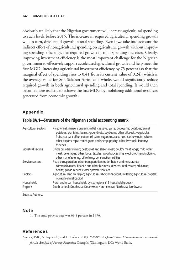
242 XINSHEN DIAO ET AL.
obviously unlikely that the Nigerian government will increase agricultural spending to such levels before 2015. The increase in required agricultural spending growth will, in turn, drive rapid growth in total spending. Even if we take into account the indirect effect of nonagricultural spending on agricultural growth without improv-ing spending effi ciency, the required growth in total spending increases. Clearly, improving investment effi ciency is the most important challenge for the Nigerian government to effectively support accelerated agricultural growth and help meet the fi rst MGD. Increasing agricultural investment effi ciency by 75 percent (so that the marginal effect of spending rises to 0.41 from its current value of 0.24), which is the average value for Sub-Saharan Africa as a whole, would signifi cantly reduce required growth in both agricultural spending and total spending. It would then become more realistic to achieve the fi rst MDG by mobilizing additional resources generated from economic growth.
Appendix
Table 8A.1—Structure of the Nigerian social accounting matrix
Agricultural sectors Rice; wheat; maize; sorghum; millet; cassava; yams; cocoyams; potatoes; sweet potatoes; plantains; beans; groundnuts; soybeans; other oilseeds; vegetables;
fruits; cocoa; coffee; cotton; oil palm; sugar; tobacco; nuts; cashew nuts; rubber; other export crops; cattle; goats and sheep; poultry; other livestock; forestry; fisheries
Industrial sectors Crude oil; other mining; beef; goat and sheep meat; poultry meat; eggs; milk; other meat; beverages; other foods; textiles; wood processing; electronic manufacturing;
other manufacturing; oil refining; construction; utilitiesService sectors Road transportation; other transportation; trade; hotels and restaurants; communications; finance and other business services; real estate; education;
health; public services; other private servicesFactors Agricultural land by region; agricultural labor; nonagricultural labor; agricultural capital; nonagricultural capitalHouseholds Rural and urban households by six regions (12 household groups)Regions South-central; Southeast; Southwest; North-central; Northeast; Northwest
Source: Authors.
Note 1. The rural poverty rate was 69.8 percent in 1996.
ReferencesAgenor, P.-R., A. Izquierdo, and H. Fofack. 2003. IMMPA: A Quantitative Macroeconomic Framework
for the Analysis of Poverty Reduction Strategies. Washington, DC: World Bank.
NIGERIA 243
Akpan, E. O. 2009. “Oil Resource Management and Food Insecurity in Nigeria.” Accessed September
16, 2011. http://erd.eui.eu/media/akpan.pdf.
CBN (Central Bank of Nigeria). 2009. “CBN Statistical Bulletin: Volume 18, December 2007: Section
B: Public Finance Statistics.” Accessed September 16, 2011. http://www.cenbank.org/OUT/
PUBLICATIONS/STATBULLETIN/STD/2009/STATISTICAL%20BULLETIN%20
VOL.%2018,%20DEC.%202007_SECTION%20B.PDF.
Fan, S., B. Yu, and A. Saurkar. 2008. “Public Spending in Developing Countries: Trends, Determination,
and Impact.” In Public Expenditures, Growth, and Poverty: Lessons from Developing Countries,
edited by S. Fan, 20–55. Baltimore: Johns Hopkins University Press.
FAO (Food and Agriculture Organization of the United Nations). 2010. FAOSTAT Statistical Database.
Accessed September 16, 2011. http://faostat.fao.org/.
Iyaniwura, J., S. Fittoh, C. Iwunor, and A. Aromolaran. 1992. Perspective Planning Nigeria: Classifi cation
Scheme for the Nigerian Social Accounting Matrix (SAM). Project Paper PP92-003. Ibadan, Nigeria:
Centre for Econometric and Allied Research (CEAR), University of Ibadan.
Nigeria, FMARD (Federal Ministry of Agriculture and Rural Development). 2008. National Food
Security Program. Lagos, Nigeria.
———. 2009. District Agricultural Production Series. Lagos, Nigeria.
Nigeria, NBS (National Bureau of Statistics). 2003. Nigerian Living Standards Survey (NLSS): 2002/03.
Lagos, Nigeria.
———. 2006. The Nigerian Statistical Factsheets on Economic and Social Development. Lagos, Nigeria.
———. 2007a. Core Welfare Monitoring Survey 2006. Lagos, Nigeria.
———. 2007b. National Accounts of Nigeria (1981–2006): Economic Reform and Government Project
(ERGP). Lagos, Nigeria.
———. 2008. Trade Statistics (1996–2005). Lagos, Nigeria.
Nigeria, NPC (National Planning Commission). 2004. National Economic Empowerment and Develop-
ment Strategy. Lagos, Nigeria.
———. 2007. National Economic Empowerment and Development Strategy II. Lagos, Nigeria.
Nin Pratt, A., and B. Yu. 2008. An Updated Look at the Recovery of Agricultural Productivity in Sub-
Saharan Africa. Discussion Paper 787. Washington, DC: International Food Policy Research
Institute.
Sanyal, P., and S. Babu. 2010. Policy Benchmarking and Tracking the Agricultural Policy Environment in
Nigeria. Nigeria Strategy Support Program (NSSP) Report 5. Abuja, Nigeria: International Food
Policy Research Institute.
World Bank. 2010. World Development Indicators. Washington, DC.

C h a p t e r 9
MalawiSamuel Benin, James Thurlow, Xinshen Diao,
Christen McCool, and Franklin Simtowe
During 2000–06, Malawi’s agricultural sector was one of the worst performing in Sub-Saharan Africa, with its gross domestic product (GDP) declining by an average 0.6 percent per year (World Bank 2010). Given that agriculture
constituted more than one-third of Malawi’s economy, its stagnation slowed overall economic growth in the country, despite nonagriculture’s stronger performance. Population growth also outpaced economic growth, causing per capita incomes to fall. By 2006 Malawi and its agricultural sector were clearly in crisis. Poverty remained high and widespread, and malnutrition and food insecurity were worsen-ing (Malawi, NSO 2005; Harrigan 2008).
It is true that Malawi is one of the most densely populated countries in Africa, and that it is prone to the detrimental effects of climate variability and extreme weather events, particularly droughts (Pauw et al. 2010). However, Malawi does have more favorable agro-ecological conditions than many other African countries (Diao et al. 2007). Indeed, agriculture’s poor performance during the early 2000s stood in stark contrast to that of the 1990s, when the sector grew by more than 7 percent per year and was the driving force behind rising per capita GDP (World Bank 2010). This rapid growth was at least partly a result of structural reforms, which, despite sequencing and implementation problems, removed many distor-
The authors thank Ian Kumwenda (Malawi Agricultural Sector Investment Programme) and David Rohrbach (World Bank–Malawi) for their comments and advice. We are grateful to Josee Randriamamonjy for her research assistance. The overall study was led by the Common Market for Eastern and Southern Africa (COMESA) and was funded by the United States Agency for International Development.
246 SAMUEL BENIN ET AL.
tionary market interventions (see Kherallah and Govindan 1999; Orr and Mwale 2001; Harrigan 2003; Dorward and Kydd 2004). These reforms addressed some of the constraints on agricultural growth, but many still remained in effect at the end of the 1990s (and some may have emerged from the reforms themselves; see Chilowa 1998). These constraints include, among others, inadequate rural infrastructure and high transaction costs (Fafchamps, Gabre-Madhin, and Minten 2005; Dorward 2006), a lack of access to credit and modern inputs (Diagne and Zeller 2001), and improper land management practices (Carr 1997).
The structural explanation for slower agricultural growth in Malawi was that land expansion was the driving force behind agricultural growth in the 1990s, and this became increasingly unsustainable because of high rural population density (and seasonal labor shortages; see Alwang and Siegel 1999; Orr 2000). Indeed, the expansion of harvested land area accounted for three-fi fths of production growth during 1997–2005, with the rest driven by yield improvements (FAO 2010). In 2006, recognizing the need for an intensifi cation strategy to address the food crisis, the Government of Malawi implemented an extensive new program to subsidize and distribute modern inputs to smallholder farmers. This effort helped generate higher agricultural and national economic growth of 6.5 and 5.5 percent per year, respectively, during 2006–09 (Sanchez, Denning, and Nziguheb. 2009; World Bank 2010; Dorward and Chirwa 2011). The 2006 program was not the fi rst attempt to publically provide farm inputs in Malawi, but previous initiatives had faced external opposition and other implementation problems (see Harrigan 2008).
Recent surveys suggest that poverty in Malawi fell between 2006 and 2009 (Malawi, NSO 2009). However, this reduction occurred mainly in urban areas and the northern region of the country. Therefore, despite higher national maize produc-tion resulting from the new input-subsidy program, there remains a pressing need for broad-based growth and poverty reduction. Domestic demand and market-ing constraints, which cause maize prices to fall when production expands, impede progress by limiting income growth for farmers. Indeed, the need for smallholder farmers in Malawi to diversify into staple crops other than maize has long been recognized (see, for example, Orr and Mwale 2001).
Given the recent successes in improving food security in many parts of rural Malawi, there is now greater scope for a more diversifi ed agricultural growth strategy (see Harrigan 2008). In this chapter we evaluate different agricultural growth paths for Malawi in terms of their ability to reduce poverty throughout the country. We also estimate the fi scal implications of the investments needed to accelerate agricultural growth. For this purpose we develop a recursive dynamic computable general equilibrium (DCGE) model of Malawi based on the one described in Chapter 2 of this volume. One of the distinctive features of this case study is its
MALAWI 247
integration of a “farm typology” within the DCGE model, which allows a higher resolution assessment of growth and poverty effects.
The chapter is structured as follows. We fi rst review the structure of Malawi’s agricultural sector and introduce the farm typology. We then describe the structure of the Malawian DCGE model and its underlying data sources. The model results are then presented for the baseline growth scenario and the accelerated agricultural growth scenarios. This is followed by the results from the investment analysis. We conclude the chapter by summarizing our fi ndings.
Agriculture in MalawiAgriculture provides a vital source of income for most Malawians. At the national level, the sector contributes more than 40 percent to GDP and 60 percent to foreign earnings (exports), and it employs three-quarters of the population.1 Malawi has one of the highest population densities in Sub-Saharan Africa, and the average land-holding size is only 1.13 hectares for rural households (World Bank 2010). Given these land constraints, we focus our discussion of the structure of agriculture around the importance of farm size in determining the cropping patterns and opportunities of farmers. Malawi can be divided into eight subnational regions or agricultural devel-opment domains (Figure 9.1). We defi ne the three rural farm household groups in each region according to the size of their landholdings. Our discussion of this typol-ogy of farmers focuses on the most important staple crop (maize) and export crop (tobacco).
Almost all farmers grow maize. However, farmers with small landholdings (less than 0.75 hectares per household) rarely grow tobacco and other export-oriented crops (Table 9.1). This group of farmers, which we call “small-scale farmers,” is characterized by small landholding sizes and few opportunities for export crop production. About one-third of Malawian farmers fall into this small-scale catego-ry, of which two-thirds reside in the three larger southern regions, Lilongwe, Machinga, and Blantyre (see Table 9A.1 in the appendix to this chapter). The aver-age landholding size for small-scale farmers is 0.69 hectares, of which 0.36 hectares is allocated to maize and 0.16 hectares to pulses. Not only are landholdings small, but average crop yields for small-scale farmers are also slightly below the national average. Small-scale farm households also tend to have lower per capita incomes and expenditures and a higher incidence of poverty. Although this farm group makes up only 30 percent of the total population, they account for 36 percent of the poor population.
Unlike small-scale farmers, farmers with more than 3 hectares of land are far more likely to engage in export-crop production, especially tobacco, tea, and sugar-
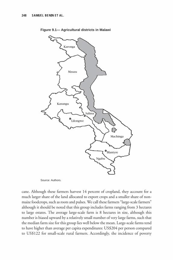
248 SAMUEL BENIN ET AL.
cane. Although these farmers harvest 14 percent of cropland, they account for a much larger share of the land allocated to export crops and a smaller share of non-maize foodcrops, such as roots and pulses. We call these farmers “large-scale farmers” although it should be noted that this group includes farms ranging from 3 hectares to large estates. The average large-scale farm is 8 hectares in size, although this number is biased upward by a relatively small number of very large farms, such that the median farm size for this group lies well below the mean. Large-scale farms tend to have higher than average per capita expenditures: US$204 per person compared to US$122 for small-scale rural farmers. Accordingly, the incidence of poverty
Lilongwe
Kasungu
Salima
Machinga
Ngabu
Mzuzu
Karonga
Blantyre
Figure 9.1— Agricultural districts in Malawi
Source: Authors.
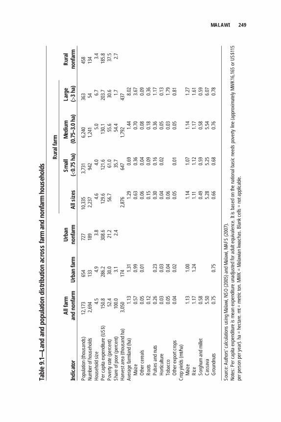
MALAWI 249
Tabl
e 9.1—
Land
and
popu
latio
n di
strib
utio
n ac
ross
farm
and
nonf
arm
hou
seho
lds
Ru
ral f
arm
Al
l far
m
Ur
ban
Sm
all
Medi
um
Larg
e Ru
ral
Indi
cato
r an
d no
nfar
m
Urba
n fa
rm
nonf
arm
Al
l size
s (<
0.75 h
a)
(0.75
–3.0
ha)
(>3 h
a)
nonf
arm
Popu
lation
(tho
usan
ds)
12,17
3 65
4 72
7 10
,335
3,731
6,2
40
363
458
Numb
er of
hous
ehold
s 2,6
94
133
189
2,237
94
2 1,2
41
54
134
Hous
ehold
size
4.5
4.9
3.8
4.6
4.0
5.0
6.7
3.4
Per c
apita
expe
nditu
re (U
S$)
150.8
28
6.2
308.6
12
9.6
121.6
13
0.1
203.7
18
5.8Po
verty
rate
(per
cent)
52
.4 30
.0 21
.2 56
.7 61
.0 55
.6 30
.6 37
.5Sh
are o
f poo
r (pe
rcent)
10
0.0
3.1
2.4
35
.7 54
.4 1.7
2.7
Harve
st ar
ea (t
hous
and h
a)
3,050
17
4
2,876
64
7 1,7
92
437
Aver
age f
arml
and (
ha)
1.13
1.31
1.2
9 0.6
9 1.4
4 8.0
2
Maize
0.5
7 0.9
9
0.63
0.36
0.70
3.67
Ot
her c
erea
ls 0.0
5 0.0
1
0.06
0.04
0.08
0.09
Ro
ots
0.12
0.15
0.09
0.18
0.36
Pu
lses a
nd nu
ts 0.2
6 0.2
3
0.30
0.16
0.36
1.17
Ho
rticult
ure
0.03
0.03
0.0
4 0.0
2 0.0
5 0.1
3
Toba
cco
0.05
0.04
0.0
6
0.03
1.79
Ot
her e
xpor
t cro
ps
0.04
0.02
0.0
5 0.0
1 0.0
5 0.8
1 Cr
op yi
elds (
mt/ha
)
Ma
ize
1.13
1.00
1.1
4 1.0
7 1.1
4 1.2
7
Rice
1.1
7 1.2
4
1.11
1.12
1.17
1.61
So
rghu
m an
d mille
t 0.5
8
0.4
9 0.5
9 0.5
8 0.5
9
Cass
ava
5.50
5.28
5.25
5.54
6.07
Gr
ound
nuts
0.75
0.75
0.6
6 0.6
8 0.7
6 0.7
8
Sour
ce: A
uthor
s’ ca
lculat
ions u
sing M
alawi
, NSO
(200
5) an
d Mala
wi, M
AFS
(200
7).
Notes
: Per
capit
a ex
pend
iture
is m
ean
expe
nditu
re u
nadju
sted
for a
dult e
quiva
lence
. It is
bas
ed o
n the
nati
onal
basic
nee
ds p
over
ty lin
e (a
ppro
ximate
ly MW
K16,1
65 o
r US$
115
per p
erso
n per
year
). ha
= he
ctare
. mt =
metr
ic ton
. MW
K =
Malaw
ian kw
acha
s. Bl
ank c
ells =
not a
pplic
able.
250 SAMUEL BENIN ET AL.
among large-scale farm households is about half that of small-scale farm households (30.6 percent compared to 61.0 percent). Given lower poverty rates and because there are only about 54,000 rural farm households with more than 3 hectares of land, only 1.7 percent of Malawi’s poor people live on large-scale farms. With the exception of tobacco, large-scale export-crop production is often concentrated in specifi c agroecological zones. For example, tea production takes place mainly in the Blantyre region, whereas sugarcane production is mainly in Salima.
Most Malawian farmers fall between the small- and large-scale groups identifi ed above. These “medium-scale” farmers, whose plots average 1.44 hectares, tend to have more diverse cropping patterns, with similar shares of land allocated to maize and nonmaize foodcrops. This group comprises 1.2 million households. Medium-scale farmers do cultivate export-oriented crops, particularly tobacco and cotton. They have larger than average household sizes, yet their per capita expenditures are above the national average. About 56 percent of people living on medium-scale farms fall below the national poverty line; this number is well above the poverty rate of large-scale farms but only slightly below that of small-scale farms. Despite the slightly lower poverty rate, the large size of this population group means that more than half of poor Malawians live on medium-scale farms in rural areas.
Finally, urban agriculturalists are an important part of Malawi’s agricultural sector. They account for almost 6 percent of harvested land (see Table 9.1). These urban farm households have cropping patterns similar to those of medium-scale rural farm households, except that they usually grow maize rather than root crops. This preference is not surprising, given the concentration of urban households in the central and southern regions of the country (roots are a more important food-crop for northern farmers) (see Table 9A.1 in the appendix to this chapter). Urban farm households also tend to be more heavily engaged in higher earning off-farm activities compared to rural households. Thus, even though farm sizes and agricul-tural incomes of urban farmers are similar to those of medium-scale rural farmers, the average per capita income is substantially higher for urban farmers. The poverty level among urban farm households is thus below that of even large-scale, nonfarm rural households, both of whose poverty rates are below the rural average.
This typology of farm and nonfarm households in each of the eight regions forms the underlying structure of the DCGE model. However, before describing the model we fi rst review Malawi’s agricultural policies and the constraints to faster growth in the sector.
The Malawian DCGE ModelA new SAM for Malawi was developed for this study to capture the country’s eco-nomic structure in 2004, including the linkages between agricultural and non-
MALAWI 251
agricultural sectors. The SAM is the main database for calibrating the Malawian DCGE model. It is built using a range of data sources, including national accounts, trade and customs data, government budgets, and household survey data. The information from these disparate sources was reconciled using cross-entropy estima-tion techniques (as described in Chapter 2).
The SAM contains detailed production information on 36 sectors, 17 of which are in agriculture (see Table 9A.2 in the appendix to this chapter). Crop production and land area data are drawn from Malawi, MAFS (2007), and crop technologies are from Malawi, MAFS (2003). When production information was unavailable for certain crops, information was taken from FAO (2010). Agricultural crops are grouped into fi ve broad groups: (1) cereal crops (for example, maize, rice, sorghum, and millet); (2) root crops (for example, cassava and potatoes); (3) pulses and nuts (such as beans, oilseeds, and groundnuts); (4) horticulture (fruits and vegetables); and (5) high-value export-oriented crops (for example, tobacco, cotton, and sugar-cane). The SAM also includes different forms of livestock, and forestry and fi sheries. These agricultural commodities are not only traded domestically and abroad but are also used as inputs by downstream activities in manufacturing, such as food and wood processing. Conversely, agricultural producers use nonagricultural inputs, such as fertilizer and transport. Nonagricultural production technologies were drawn from the input–output table in Chulu and Wobst (2001). The SAM database on production technologies and linkages allows the DCGE model to evaluate economywide impacts of growth in different agricultural crops and subsectors.
The DCGE model also captures heterogeneity in spatial production patterns. Rural agricultural production is disaggregated into Malawi’s eight main agro-ecological regions (see Figure 9.1) and into small-, medium-, and large-scale farmer groups (based on the farm typology described in the previous section). To capture the importance and unique circumstances of urban agriculture, urban agricultural production is treated as a separate region. Thus, nine subnational regions are identi-fi ed in the model (eight rural and one urban) and have different initial cropping patterns.
Each group of farmers in each region responds to changes in production tech-nology, commodity demand, and relative prices by reallocating their agricultural lands to different crops in order to maximize income. These representative farmers also reallocate labor and capital between farm and nonfarm activities, including livestock and fi shing, wage employment on larger farms, and migration to non-agricultural work in more urbanized sectors. Labor in the Malawi model is separated into categories, including region-specifi c family farmworkers, national unskilled labor working both on and off the farm, and national skilled non-farmworkers.
By capturing farm-level information across subnational regions, the DCGE model can assess growth effects at the national level while also taking into account
252 SAMUEL BENIN ET AL.
the microlevel decisionmaking typically associated with more detailed farm models. This linking of farm-level and economywide models is an extension of the DCGE model beyond what is used in earlier case studies in this volume. The Malawi model is an ideal tool for capturing regional and intersectoral production linkages. However, the output from each region is traded in national markets because of a lack of infor-mation on intranational trade fl ows in Malawi.
Finally, the DCGE model endogenously estimates the impact of alternative growth paths on the incomes of various household groups. These household groups include both farm and nonfarm households and are also disaggregated across the nine regions and rural and urban areas. The rural farm households are further sepa-rated by land size into small-, medium- and large-scale farm households. The income elasticities determining these household groups’ marginal budget shares are estimated using the 2004–05 Integrated Household Survey (IHS2) (Malawi, NSO 2005) (see Table 9A.3 in the appendix to this chapter). Each household in the survey is also linked to its corresponding representative household in the DCGE model. This linkage takes place in the microsimulation module in which changes in repre-sentative households’ consumption and prices in the DCGE model are passed down to their matching households in the survey, where total consumption expenditures are recalculated. The revised level of per capita expenditure for each survey house-hold is compared to the offi cial poverty line, and standard poverty measures are recalculated. Thus, poverty is measured in the same way as in offi cial poverty esti-mates, and changes in poverty estimated by the DCGE model refl ect differences in household consumption patterns and income distribution captured in IHS2.
Baseline Growth ScenarioWe fi rst evaluate poverty reduction under Malawi’s current growth trends and pat-terns, which we call the “baseline” scenario. As mentioned above, Malawi experi-enced modest national growth and negative agricultural growth in 2000–06. If we expand the period to 1990–2005, national GDP growth is still low at 2.8 percent (Malawi, NSO 2007). However, agriculture’s growth rate over this longer period was 4.6 percent per year. Considering that agricultural growth in Malawi is erratic due to climate variability and that average growth rate has been particularly low in recent years, we target a more modest agricultural growth rate in the baseline scenario for agricultural GDP: 2.8 percent per year for 2005–15 (Table 9.2). We therefore select the period prior to the new input subsidy program as the baseline, so that the accelerated growth scenarios, which are reported later in this chapter, will refl ect in part the successes of this program. The changes in crop yields and land area needed to support the baseline level of agricultural GDP growth are reported in Table 9.3. The nonagricultural sectors are expected to maintain a similar growth
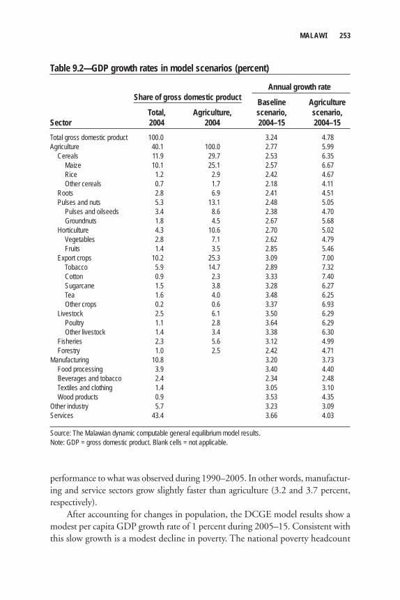
MALAWI 253
performance to what was observed during 1990–2005. In other words, manufactur-ing and service sectors grow slightly faster than agriculture (3.2 and 3.7 percent, respectively).
After accounting for changes in population, the DCGE model results show a modest per capita GDP growth rate of 1 percent during 2005–15. Consistent with this slow growth is a modest decline in poverty. The national poverty headcount
Table 9.2—GDP growth rates in model scenarios (percent)
Annual growth rate
Baseline Agriculture Total, Agriculture, scenario, scenario,Sector 2004 2004 2004–15 2004–15Total gross domestic product 100.0 3.24 4.78Agriculture 40.1 100.0 2.77 5.99 Cereals 11.9 29.7 2.53 6.35 Maize 10.1 25.1 2.57 6.67 Rice 1.2 2.9 2.42 4.67 Other cereals 0.7 1.7 2.18 4.11 Roots 2.8 6.9 2.41 4.51 Pulses and nuts 5.3 13.1 2.48 5.05 Pulses and oilseeds 3.4 8.6 2.38 4.70 Groundnuts 1.8 4.5 2.67 5.68 Horticulture 4.3 10.6 2.70 5.02 Vegetables 2.8 7.1 2.62 4.79 Fruits 1.4 3.5 2.85 5.46 Export crops 10.2 25.3 3.09 7.00 Tobacco 5.9 14.7 2.89 7.32 Cotton 0.9 2.3 3.33 7.40 Sugarcane 1.5 3.8 3.28 6.27 Tea 1.6 4.0 3.48 6.25 Other crops 0.2 0.6 3.37 6.93 Livestock 2.5 6.1 3.50 6.29 Poultry 1.1 2.8 3.64 6.29 Other livestock 1.4 3.4 3.38 6.30 Fisheries 2.3 5.6 3.12 4.99 Forestry 1.0 2.5 2.42 4.71Manufacturing 10.8 3.20 3.73 Food processing 3.9 3.40 4.40 Beverages and tobacco 2.4 2.34 2.48 Textiles and clothing 1.4 3.05 3.10 Wood products 0.9 3.53 4.35Other industry 5.7 3.23 3.09Services 43.4 3.66 4.03
Source: The Malawian dynamic computable general equilibrium model results.Note: GDP = gross domestic product. Blank cells = not applicable.
Share of gross domestic product
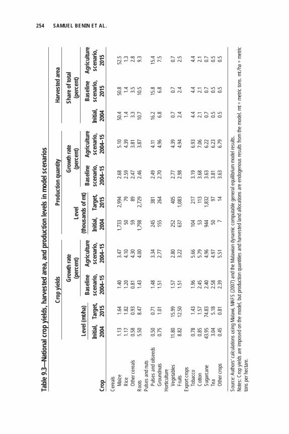
254 SAMUEL BENIN ET AL.
Tabl
e 9.3—
Natio
nal c
rop
yield
s, ha
rves
ted
area
, and
pro
duct
ion
levels
in m
odel
scen
ario
s
Cr
op yi
elds
Prod
uctio
n qu
antit
y Ha
rves
ted
area
Grow
th ra
te
Leve
l Gr
owth
rate
Sh
are o
f tot
al
(p
erce
nt)
(thou
sand
s of m
t) (p
erce
nt)
(per
cent
)
Ba
selin
e Ag
ricul
ture
Ba
selin
e Ag
ricul
ture
Base
line
Agric
ultu
re
Initi
al,
Targ
et,
scen
ario
, sc
enar
io,
Initi
al,
Targ
et,
scen
ario
, sc
enar
io,
Initi
al,
scen
ario
, sc
enar
io,
Crop
20
04
2015
20
04–1
5 20
04–1
5 20
04
2015
20
04–1
5 20
04–1
5 20
04
2015
20
15Ce
reals
Maize
1.1
3 1.6
4 1.4
0 3.4
7 1,7
33
2,994
2.6
8 5.1
0 50
.4 50
.8 52
.5
Rice
1.1
7 1.8
2 1.2
0 4.1
0 50
79
2.5
9 4.3
9 1.4
1.4
1.3
Ot
her c
erea
ls
0.58
0.93
0.81
4.30
59
89
2.47
3.81
3.3
3.5
2.8Ro
ots
5.50
8.47
1.43
4.00
1,798
2,7
29
2.46
3.87
10.7
10.5
9.3Pu
lses a
nd nu
ts
Pu
lses a
nd oi
lseed
s 0.5
0 0.7
1 1.4
8 3.3
4 24
5 38
1 2.4
9 4.1
1 16
.2 15
.8 15
.4
Grou
ndnu
ts 0.7
5 1.0
1 1.5
1 2.7
7 15
5 26
4 2.7
0 4.9
6 6.8
6.8
7.5
Hortic
ultur
e
Ve
getab
les
11.80
15
.99
1.57
2.80
252
405
2.77
4.39
0.7
0.7
0.7
Fruit
s 8.8
2 12
.50
1.51
3.22
637
1,083
2.9
8 4.9
4 2.4
2.4
2.5
Expo
rt cro
ps
Toba
cco
0.78
1.43
1.96
5.66
104
217
3.19
6.93
4.4
4.4
4.4
Cotto
n 0.8
5 1.5
7 2.4
5 5.7
9 53
11
3 3.6
8 7.0
6 2.1
2.1
2.1
Su
garca
ne
43.95
74
.83
2.40
4.96
944
1,832
3.6
3 6.2
2 0.7
0.7
0.7
Te
a 3.0
4 5.1
8 2.5
8 4.9
7 50
97
3.8
1 6.2
3 0.5
0.5
0.5
Ot
her c
rops
0.4
5 0.8
1 2.3
9 5.5
1 7
14
3.63
6.79
0.5
0.5
0.5
Sour
ce: A
uthor
s’ ca
lculat
ions u
sing M
alawi
, MAF
S (2
007)
and t
he M
alawi
an dy
nami
c com
putab
le ge
nera
l equ
ilibriu
m mo
del re
sults
.No
tes: C
rop
yields
are
impo
sed
on th
e mo
del, b
ut pr
oduc
tion
quan
tities
and
har
veste
d lan
d all
ocati
ons a
re e
ndog
enou
s res
ults f
rom
the m
odel.
mt =
metr
ic ton
s. mt
/ ha
= me
tric
tons p
er he
ctare
.
Leve
l (m
t/ha)
Leve
l(th
ousa
nds o
f mt)
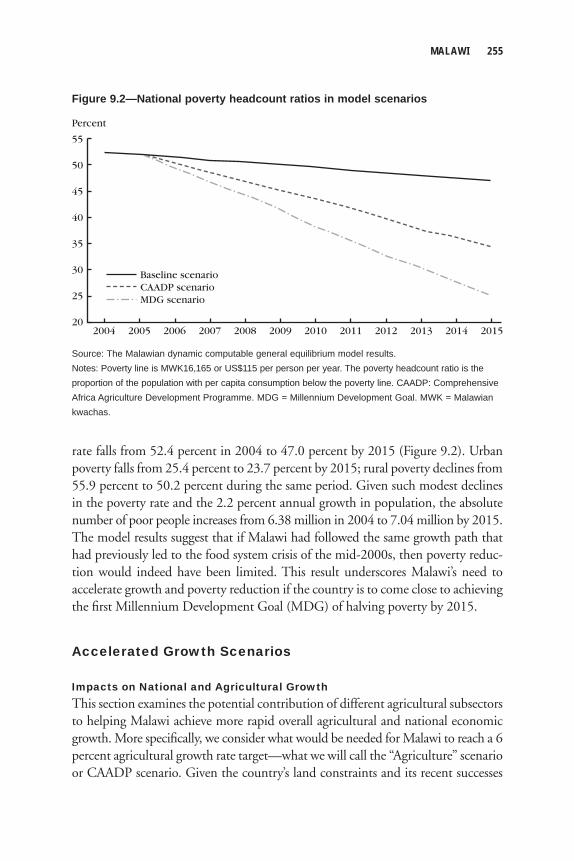
MALAWI 255
rate falls from 52.4 percent in 2004 to 47.0 percent by 2015 (Figure 9.2). Urban poverty falls from 25.4 percent to 23.7 percent by 2015; rural poverty declines from 55.9 percent to 50.2 percent during the same period. Given such modest declines in the poverty rate and the 2.2 percent annual growth in population, the absolute number of poor people increases from 6.38 million in 2004 to 7.04 million by 2015. The model results suggest that if Malawi had followed the same growth path that had previously led to the food system crisis of the mid-2000s, then poverty reduc-tion would indeed have been limited. This result underscores Malawi’s need to accelerate growth and poverty reduction if the country is to come close to achieving the fi rst Millennium Development Goal (MDG) of halving poverty by 2015.
Accelerated Growth Scenarios
Impacts on National and Agricultural GrowthThis section examines the potential contribution of different agricultural subsectors to helping Malawi achieve more rapid overall agricultural and national economic growth. More specifi cally, we consider what would be needed for Malawi to reach a 6 percent agricultural growth rate target—what we will call the “Agriculture” scenario or CAADP scenario. Given the country’s land constraints and its recent successes
Percent
55
Baseline scenario
20
50
45
40
35
30
25
201520142013201220112010200920082007200620052004
CAADP scenarioMDG scenario
Figure 9.2—National poverty headcount ratios in model scenarios
Source: The Malawian dynamic computable general equilibrium model results.Notes: Poverty line is MWK16,165 or US$115 per person per year. The poverty headcount ratio is the proportion of the population with per capita consumption below the poverty line. CAADP: ComprehensiveAfrica Agriculture Development Programme. MDG = Millennium Development Goal. MWK = Malawian kwachas.
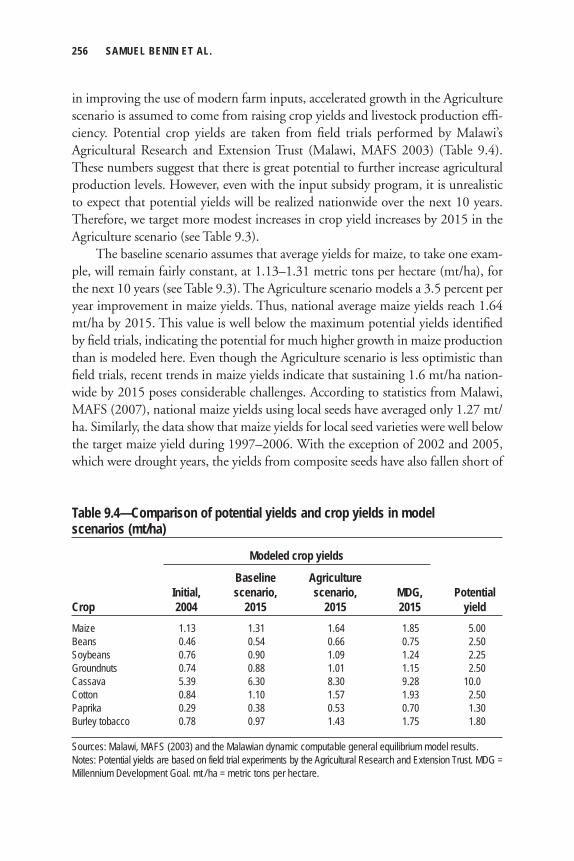
256 SAMUEL BENIN ET AL.
in improving the use of modern farm inputs, accelerated growth in the Agriculture scenario is assumed to come from raising crop yields and livestock production effi -ciency. Potential crop yields are taken from fi eld trials performed by Malawi’s Agricultural Research and Extension Trust (Malawi, MAFS 2003) (Table 9.4). These numbers suggest that there is great potential to further increase agricultural production levels. However, even with the input subsidy program, it is unrealistic to expect that potential yields will be realized nationwide over the next 10 years. Therefore, we target more modest increases in crop yield increases by 2015 in the Agriculture scenario (see Table 9.3).
The baseline scenario assumes that average yields for maize, to take one exam-ple, will remain fairly constant, at 1.13–1.31 metric tons per hectare (mt/ha), for the next 10 years (see Table 9.3). The Agriculture scenario models a 3.5 percent per year improvement in maize yields. Thus, national average maize yields reach 1.64 mt/ha by 2015. This value is well below the maximum potential yields identifi ed by fi eld trials, indicating the potential for much higher growth in maize production than is modeled here. Even though the Agriculture scenario is less optimistic than fi eld trials, recent trends in maize yields indicate that sustaining 1.6 mt/ha nation-wide by 2015 poses considerable challenges. According to statistics from Malawi, MAFS (2007), national maize yields using local seeds have averaged only 1.27 mt/ha. Similarly, the data show that maize yields for local seed varieties were well below the target maize yield during 1997–2006. With the exception of 2002 and 2005, which were drought years, the yields from composite seeds have also fallen short of
Table 9.4—Comparison of potential yields and crop yields in model scenarios (mt/ha)
Modeled crop yields
Baseline Agriculture Initial, scenario, scenario, MDG, PotentialCrop 2004 2015 2015 2015 yieldMaize 1.13 1.31 1.64 1.85 5.00Beans 0.46 0.54 0.66 0.75 2.50Soybeans 0.76 0.90 1.09 1.24 2.25Groundnuts 0.74 0.88 1.01 1.15 2.50Cassava 5.39 6.30 8.30 9.28 10.0Cotton 0.84 1.10 1.57 1.93 2.50Paprika 0.29 0.38 0.53 0.70 1.30Burley tobacco 0.78 0.97 1.43 1.75 1.80
Sources: Malawi, MAFS (2003) and the Malawian dynamic computable general equilibrium model results.Notes: Potential yields are based on field trial experiments by the Agricultural Research and Extension Trust. MDG = Millennium Development Goal. mt / ha = metric tons per hectare.
MALAWI 257
the target yield. Thus, the government would not only have to improve the distribu-tion of hybrid and composite seeds but also improve current farming practices and the distribution of other inputs if it is to help farmers reach yield potentials by 2015. For these reasons, 1.64 mt/ha is considered a reasonable, albeit still challenging, maize yield target for the Agriculture scenario.
Agriculture’s current poor performance means that achieving the 6 percent annual agricultural growth target poses a substantial challenge. Malawi would need fi rst to double its 1990–2006 agricultural growth rate and then sustain this rate of growth over a 10-year period. However, modeling results indicate that, given its crop yield and agricultural productivity potentials, Malawi could achieve an average agricultural growth rate of 6 percent during 2005–15. Because agriculture forms such a large part of the Malawian economy, this acceleration in agricultural growth would signifi cantly increase the national GDP growth rate from its current 3.2 percent to 4.8 percent per year. Faster agricultural growth will also stimulate addi-tional growth in the nonagricultural sectors, both by increasing fi nal demand for nonagricultural goods and by lowering input prices and fostering downstream pro-cessing. For instance, in the Agriculture scenario, the GDP growth rate in the food-processing sector increases from 3.4 to 4.4 percent per year. Expanding agriculture also generates additional demand for chemicals and transport services, which further stimulates manufacturing and service sector growth. Accelerating agricultural growth therefore has strong growth-linkage effects for the whole economy.
Impacts on Household Income and Poverty The acceleration of the agricultural growth rate to 6 percent per year and the spill-over effects into nonagriculture cause poverty to decline by a further 12.5 percentage points. This result is shown in Figure 9.1, where the share of Malawi’s population below the poverty line is 34.5 percent by 2015 in the Agriculture scenario compared to 47.0 percent in the baseline. Thus, taking population growth into account, achieving the target of a 6 percent agricultural growth rate lifts an additional 1.88 million people above the poverty line by 2015. This would be suffi cient to substan-tially reduce the absolute number of poor people in Malawi by 2015. Food security would also improve, with annual average per capita cereal consumption rising from 153.5 to 176.7 kilograms by 2015.
Faster agricultural growth would benefi t most households, although rural households benefi t more than urban households in terms of increases in per capita real income. Table 9.5 shows that per capita income of rural households grows by 2.0 percent annually in the Agriculture scenario and by 1.2 percent for urban house-holds. However, in rural areas, the large-scale farmer group benefi ts the most, as this group’s per capita income grows at 2.5 percent per year. In contrast, the income growth rate for the small-scale farmer group is 2.0 percent. This difference is con-
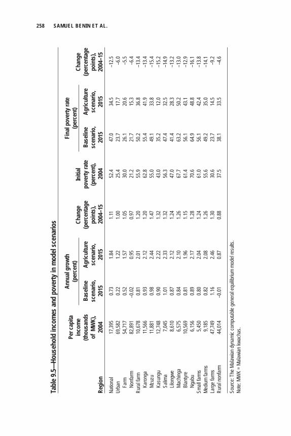
258 SAMUEL BENIN ET AL.
Tabl
e 9.5—
Hous
ehol
d in
com
es an
d po
verty
in m
odel
scen
ario
s
Pe
r cap
ita
inco
me
Chan
ge
Initi
al
Ch
ange
(th
ousa
nds
Base
line
Agric
ultu
re
(per
cent
age
pove
rty ra
te
Base
line
Agric
ultu
re
(per
cent
age
of
MW
K),
scen
ario
, sc
enar
io,
poin
ts),
(per
cent
), sc
enar
io,
scen
ario
, po
ints
),Re
gion
20
04
2015
20
15
2004
–15
2004
20
15
2015
20
04–1
5Na
tiona
l 17
,395
0.73
1.84
1.11
52.4
47.0
34.5
–12.5
Urba
n 69
,582
0.22
1.22
1.00
25.4
23.7
17.7
–6.0
Fa
rm
54,71
7 0.5
2 1.5
7 1.0
5 30
.0 26
.1 20
.6 –5
.5
Nonfa
rm
82,89
1 –0
.02
0.95
0.97
21.2
21.7
15.3
–6.4
Rura
l farm
10
,678
0.81
2.01
1.20
55.9
50.2
36.8
–13.4
Ka
rong
a 11
,566
0.93
2.12
1.20
62.8
55.4
41.9
–13.4
Mz
uzu
11,88
1 0.9
8 2.4
4 1.4
7 55
.0 49
.1 33
.8 –1
5.4
Kasu
ngu
12,74
8 0.9
0 2.2
2 1.3
2 43
.0 35
.2 12
.0 –1
5.2
Salim
a 7,0
45
1.01
2.33
1.32
56.3
47.4
32.5
–14.9
Lil
ongw
e 8,6
10
0.87
2.12
1.24
47.0
41.4
28.3
–13.2
Ma
ching
a 6,5
75
0.84
2.10
1.26
67.7
63.2
50.2
–13.0
Bl
antyr
e 10
,569
0.81
1.96
1.15
61.4
56.1
43.1
–12.9
Ng
abu
6,156
0.8
9 2.1
7 1.2
8 70
.6 64
.9 48
.8 –1
6.1Sm
all fa
rms
5,450
0.8
0 2.0
4 1.2
4 61
.0 56
.1 42
.4 –1
3.8Me
dium
farms
9,1
85
0.82
2.08
1.26
55.6
49.2
35.0
–14.1
Larg
e far
ms
47,74
9 1.1
6 2.4
6 1.3
0 30
.6 23
.7 14
.5 –9
.2Ru
ral n
onfar
m 44
,014
–0.01
0.8
7 0.8
8 37
.5 38
.1 33
.5 –4
.6
Sour
ce: T
he M
alawi
an dy
nami
c com
putab
le ge
nera
l equ
ilibriu
m mo
del re
sults
.No
te: M
WK
= Ma
lawian
kwac
has.
Annu
al gr
owth
(per
cent
)Fi
nal p
over
ty ra
te(p
erce
nt)
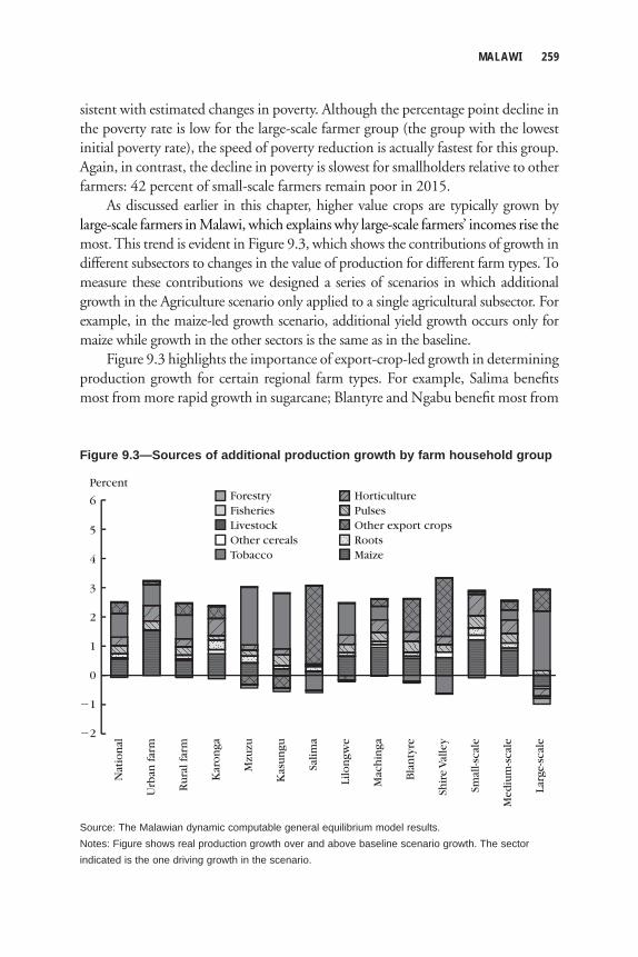
MALAWI 259
sistent with estimated changes in poverty. Although the percentage point decline in the poverty rate is low for the large-scale farmer group (the group with the lowest initial poverty rate), the speed of poverty reduction is actually fastest for this group. Again, in contrast, the decline in poverty is slowest for smallholders relative to other farmers: 42 percent of small-scale farmers remain poor in 2015.
As discussed earlier in this chapter, higher value crops are typically grown by large-scale farmers in Malawi, which explains why large-scale farmers’ incomes rise the most. This trend is evident in Figure 9.3, which shows the contributions of growth in different subsectors to changes in the value of production for different farm types. To measure these contributions we designed a series of scenarios in which additional growth in the Agriculture scenario only applied to a single agricultural subsector. For example, in the maize-led growth scenario, additional yield growth occurs only for maize while growth in the other sectors is the same as in the baseline.
Figure 9.3 highlights the importance of export-crop-led growth in determining production growth for certain regional farm types. For example, Salima benefi ts most from more rapid growth in sugarcane; Blantyre and Ngabu benefi t most from
Percent
5
�2
4
6
3
2
1
0
�1
Nat
ion
al
Urb
an f
arm
Ru
ral f
arm
Kar
on
ga
Mzu
zu
Kas
un
gu
Salim
a
Lilo
ngw
e
Mac
hin
ga
Bla
nty
re
Shir
e V
alle
y
Smal
l-sca
le
Med
ium
-sca
le
Larg
e-sc
ale
Tobacco
FisheriesForestry
Other cerealsLivestock
Maize
PulsesHorticulture
RootsOther export crops
Figure 9.3—Sources of additional production growth by farm household group
Source: The Malawian dynamic computable general equilibrium model results.Notes: Figure shows real production growth over and above baseline scenario growth. The sector indicated is the one driving growth in the scenario.
260 SAMUEL BENIN ET AL.
expanding tea and cotton production; and Lilongwe, Kasungu, and Mzuzu benefi t most from faster tobacco growth. Taken together, these fi ndings indicate that increases in export crops could generate the same additional agricultural production as maize-led growth, at least at the national level.
The fi gure also indicates that the sources of additional production vary across farm types. Not surprisingly, farmers who already depend heavily on maize tend to benefi t more from maize-led growth. Such benefi t comes from not only productivity gains in maize production but also from additional growth in other crops because of the reallocation of cropland. When maize production increases, prices for maize may fall as increased incomes for maize growers are spent on consumption of other products. In response to changes in relative prices, farmers may allocate less land to maize and grow more of other crops. The DCGE model captures both direct and indirect effects when assessing the effects of improved yields in different subsectors.
The model also takes into account potential competition for limited agricul-tural resources. For example, farmers in Salima and Ngabu (Shire Valley) appear to be hurt by tobacco-led growth (Figure 9.4). However, this decline in production for nontobacco-producing regions refl ects the shift in nationally mobile resources (that is, unskilled labor and agricultural capital) to the production of export crops. The model captures how the increased growth potential for tobacco causes farm labor and capital to shift to the production of export crops on large-scale farms, causing declines in production by other farm types. However, these resource reallocations or indirect effects from export-crop-led growth are relatively small. Overall, the model indicates that rural and small-scale farms would benefi t greatly from faster agricultural growth.
Figure 9.4 shows that rising incomes for rural farm households in Mzuzu and Kasungu are driven by growth in tobacco, with almost three-quarters of additional incomes being generated by this crop alone. In contrast, households in Salima benefi t more from expanded sugarcane production. This is not surprising, given the current concentration of Malawi’s sugarcane production among large-scale farmers in this region.
Decomposing Agriculture’s Impacts on Poverty The discussion above highlighted the potential contributions of agricultural sub-sectors to accelerating agricultural growth and poverty reduction. However, the different sizes of these subsectors make it diffi cult to compare the effectiveness of sectoral growth in reducing poverty. Understanding how poverty–growth linkages vary at the subsector and household levels is important for designing pro-poor growth strategies. In this section, we calculate poverty–growth elasticities that allow us to compare the pro-poorness of growth in alternative subsectors. More specifi -
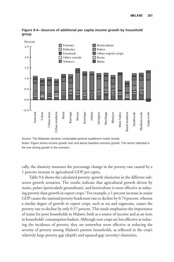
MALAWI 261
cally, the elasticity measures the percentage change in the poverty rate caused by a 1 percent increase in agricultural GDP per capita.
Table 9.6 shows the calculated poverty–growth elasticities in the different sub-sector growth scenarios. The results indicate that agricultural growth driven by maize, pulses (particularly groundnuts), and horticulture is more effective at reduc-ing poverty than growth in export crops.2 For example, a 1 percent increase in maize GDP causes the national poverty headcount rate to decline by 0.74 percent, whereas a similar degree of growth in export crops, such as tea and sugarcane, causes the poverty rate to decline by only 0.57 percent. This result emphasizes the importance of maize for poor households in Malawi, both as a source of income and as an item in households’ consumption baskets. Although root crops are less effective at reduc-ing the incidence of poverty, they are somewhat more effective at reducing the severity of poverty among Malawi’s poorest households, as refl ected in the crop’s relatively large poverty gap (depth) and squared-gap (severity) elasticities.
Percent
�0.5
2.5
2.0
1.5
1.0
0.0
0.5
Nat
ion
al
Urb
an
Ru
ral
Kar
on
ga
Mzu
zu
Urb
an f
arm
Urb
an n
on
farm
Kas
un
gu
Salim
a
Lilo
ngw
e
Mac
hin
ga
Bla
nty
re
Shir
e V
alle
y
Ru
ral n
on
farm
Smal
l-sca
le
Med
ium
-sca
le
Larg
e-sc
ale
Tobacco
FisheriesForestry
Other cerealsLivestock
Maize
PulsesHorticulture
RootsOther export crops
Figure 9.4—Sources of additional per capita income growth by household group
Source: The Malawian dynamic computable general equilibrium model results.Notes: Figure shows income growth over and above baseline scenario growth. The sector indicated is the one driving growth in the scenario.
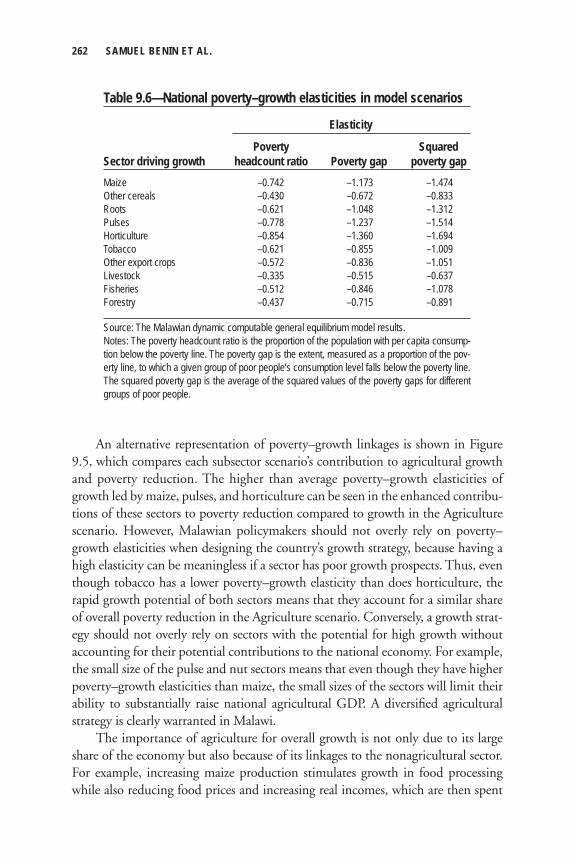
262 SAMUEL BENIN ET AL.
An alternative representation of poverty–growth linkages is shown in Figure 9.5, which compares each subsector scenario’s contribution to agricultural growth and poverty reduction. The higher than average poverty–growth elasticities of growth led by maize, pulses, and horticulture can be seen in the enhanced contribu-tions of these sectors to poverty reduction compared to growth in the Agriculture scenario. However, Malawian policymakers should not overly rely on poverty–growth elasticities when designing the country’s growth strategy, because having a high elasticity can be meaningless if a sector has poor growth prospects. Thus, even though tobacco has a lower poverty–growth elasticity than does horticulture, the rapid growth potential of both sectors means that they account for a similar share of overall poverty reduction in the Agriculture scenario. Conversely, a growth strat-egy should not overly rely on sectors with the potential for high growth without accounting for their potential contributions to the national economy. For example, the small size of the pulse and nut sectors means that even though they have higher poverty–growth elasticities than maize, the small sizes of the sectors will limit their ability to substantially raise national agricultural GDP. A diversifi ed agricultural strategy is clearly warranted in Malawi.
The importance of agriculture for overall growth is not only due to its large share of the economy but also because of its linkages to the nonagricultural sector. For example, increasing maize production stimulates growth in food processing while also reducing food prices and increasing real incomes, which are then spent
Table 9.6—National poverty–growth elasticities in model scenarios
Elasticity
Poverty SquaredSector driving growth headcount ratio Poverty gap poverty gapMaize –0.742 –1.173 –1.474Other cereals –0.430 –0.672 –0.833Roots –0.621 –1.048 –1.312Pulses –0.778 –1.237 –1.514Horticulture –0.854 –1.360 –1.694Tobacco –0.621 –0.855 –1.009Other export crops –0.572 –0.836 –1.051Livestock –0.335 –0.515 –0.637Fisheries –0.512 –0.846 –1.078Forestry –0.437 –0.715 –0.891
Source: The Malawian dynamic computable general equilibrium model results.Notes: The poverty headcount ratio is the proportion of the population with per capita consump-tion below the poverty line. The poverty gap is the extent, measured as a proportion of the pov-erty line, to which a given group of poor people’s consumption level falls below the poverty line. The squared poverty gap is the average of the squared values of the poverty gaps for different groups of poor people.
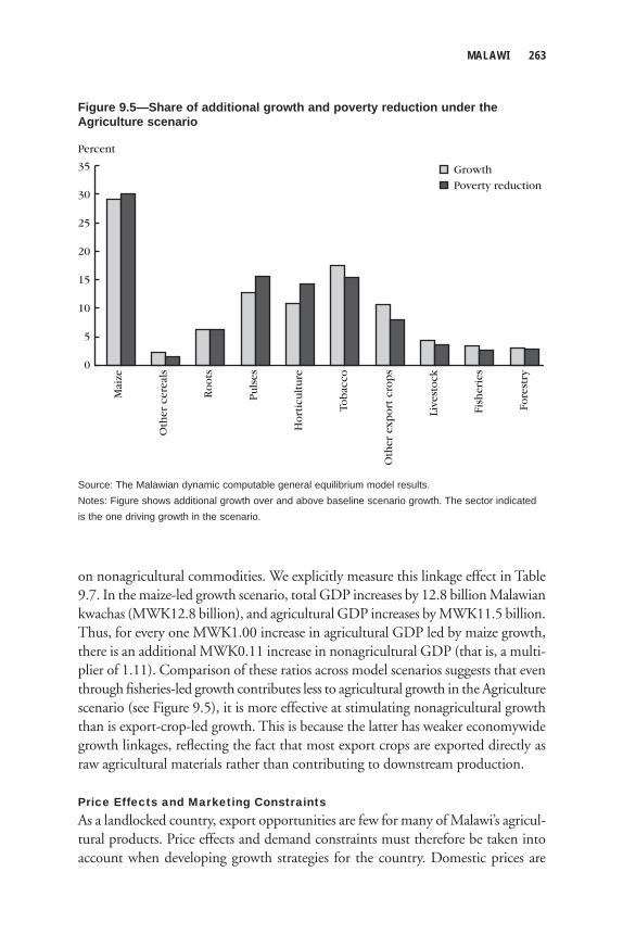
MALAWI 263
on nonagricultural commodities. We explicitly measure this linkage effect in Table 9.7. In the maize-led growth scenario, total GDP increases by 12.8 billion Malawian kwachas (MWK12.8 billion), and agricultural GDP increases by MWK11.5 billion. Thus, for every one MWK1.00 increase in agricultural GDP led by maize growth, there is an additional MWK0.11 increase in nonagricultural GDP (that is, a multi-plier of 1.11). Comparison of these ratios across model scenarios suggests that even through fi sheries-led growth contributes less to agricultural growth in the Agriculture scenario (see Figure 9.5), it is more effective at stimulating nonagricultural growth than is export-crop-led growth. This is because the latter has weaker economywide growth linkages, refl ecting the fact that most export crops are exported directly as raw agricultural materials rather than contributing to downstream production.
Price Effects and Marketing ConstraintsAs a landlocked country, export opportunities are few for many of Malawi’s agricul-tural products. Price effects and demand constraints must therefore be taken into account when developing growth strategies for the country. Domestic prices are
Mai
ze
Oth
er c
erea
ls
Ho
rtic
ult
ure
Tob
acco
Oth
er e
xp
ort
cro
ps
Ro
ots
Pu
lses
Live
sto
ck
Fish
erie
s
Fore
stry
Poverty reduction
Growth
Percent
35
0
30
25
20
15
10
5
Figure 9.5—Share of additional growth and poverty reduction under the Agriculture scenario
Source: The Malawian dynamic computable general equilibrium model results.Notes: Figure shows additional growth over and above baseline scenario growth. The sector indicated is the one driving growth in the scenario.
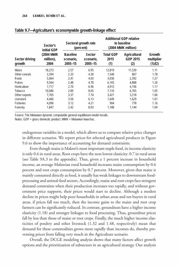
264 SAMUEL BENIN ET AL.
endogenous variables in a model, which allows us to compare relative price changes in different scenarios. We report prices for selected agricultural products in Figure 9.6 to show the importance of accounting for demand constraints.
Even though maize is Malawi’s most important staple food, its income elasticity is only 0.6 in rural areas. Root crops have the next lowest elasticity: 0.7 in rural areas (see Table 9A.3 in the appendix). Thus, given a 1 percent increase in household income, an average Malawian rural household increases maize consumption by 0.6 percent and root crops consumption by 0.7 percent. Moreover, given that maize is mainly consumed directly as food, it usually has weak linkages to downstream food-processing and animal-feed sectors. Accordingly, maize and root crops face stringent demand constraints when their production increases too rapidly, and without gov-ernment price supports, their prices would start to decline. Although a modest decline in prices might help poor households in urban areas and net buyers in rural areas, if prices fall too much, then the income gains to the maize and root crop farmers can be signifi cantly reduced. In contrast, groundnuts have a higher income elasticity (1.18) and stronger linkages to food processing. Thus, groundnut prices fall by less than those of maize or root crops. Finally, the much higher income elas-ticities of poultry and other livestock (1.32 and 1.48, respectively) mean that demand for these commodities grows more rapidly than incomes do, thereby pre-venting prices from falling very much in the Agriculture scenario.
Overall, the DCGE modeling analysis shows that many factors affect growth options and the prioritization of subsectors in an agricultural strategy. Our analysis
Table 9.7—Agriculture’s economywide growth-linkage effect
Sector’s initial GDP (2004 MWK Baseline Sector Total GDP Agricultural GrowthSector driving million), scenario, scenario, 2015 GDP 2015 multipliergrowth 2004 2005–15 2005–15 (1) (2) (1)/(2)Maize 18,273 2.57 6.95 12,819 11,539 1.11Other cereals 3,394 2.33 4.30 1,540 867 1.78Roots 5,064 2.41 4.03 3,036 2,392 1.27Pulses 9,564 2.48 4.78 6,165 4,888 1.26Horticulture 7,717 2.70 6.96 4,915 4,196 1.17Tobacco 10,686 2.89 8.65 7,133 6,765 1.05Other exports 7,765 3.37 7.74 3,421 3,218 1.06Livestock 4,466 3.50 6.13 1,649 1,629 1.01Fisheries 4,096 3.12 4.21 904 778 1.16Forestry 1,847 2.42 8.03 1,188 1,144 1.04
Source: The Malawian dynamic computable general equilibrium model results.Notes: GDP = gross domestic product. MWK = Malawian kwachas.
Sectoral growth rate (percent)
Additional GDP relative to baseline
(2004 MWK million)
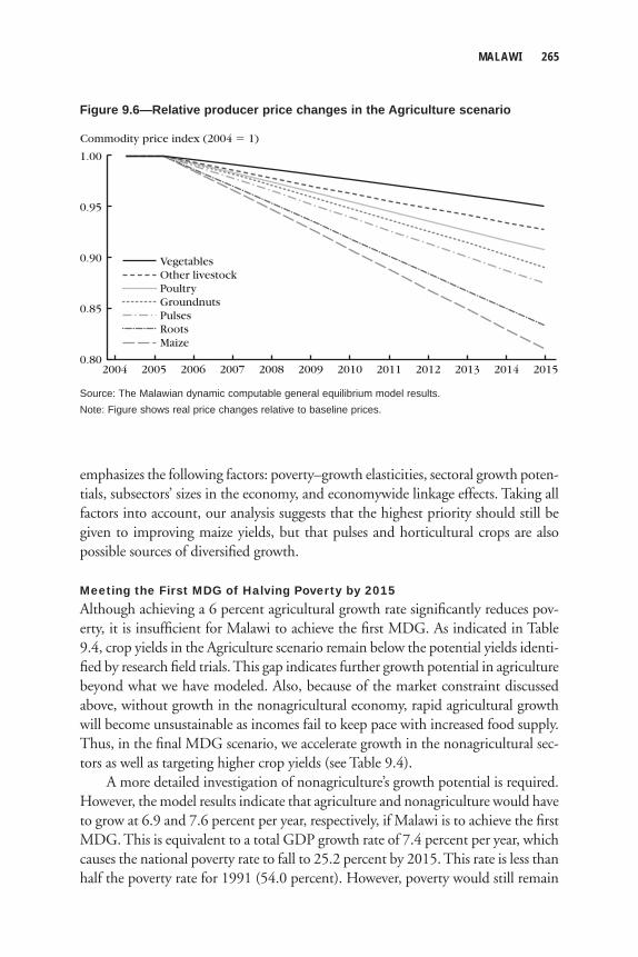
MALAWI 265
emphasizes the following factors: poverty–growth elasticities, sectoral growth poten-tials, subsectors’ sizes in the economy, and economywide linkage effects. Taking all factors into account, our analysis suggests that the highest priority should still be given to improving maize yields, but that pulses and horticultural crops are also possible sources of diversifi ed growth.
Meeting the First MDG of Halving Poverty by 2015Although achieving a 6 percent agricultural growth rate signifi cantly reduces pov-erty, it is insuffi cient for Malawi to achieve the fi rst MDG. As indicated in Table 9.4, crop yields in the Agriculture scenario remain below the potential yields identi-fi ed by research fi eld trials. This gap indicates further growth potential in agriculture beyond what we have modeled. Also, because of the market constraint discussed above, without growth in the nonagricultural economy, rapid agricultural growth will become unsustainable as incomes fail to keep pace with increased food supply. Thus, in the fi nal MDG scenario, we accelerate growth in the nonagricultural sec-tors as well as targeting higher crop yields (see Table 9.4).
A more detailed investigation of nonagriculture’s growth potential is required. However, the model results indicate that agriculture and nonagriculture would have to grow at 6.9 and 7.6 percent per year, respectively, if Malawi is to achieve the fi rst MDG. This is equivalent to a total GDP growth rate of 7.4 percent per year, which causes the national poverty rate to fall to 25.2 percent by 2015. This rate is less than half the poverty rate for 1991 (54.0 percent). However, poverty would still remain
Commodity price index (2004 � 1)
1.00
0.80
0.95
0.90
0.85
VegetablesOther livestock
Pulses
PoultryGroundnuts
RootsMaize
201520142013201220112010200920082007200620052004
Figure 9.6—Relative producer price changes in the Agriculture scenario
Source: The Malawian dynamic computable general equilibrium model results.Note: Figure shows real price changes relative to baseline prices.
266 SAMUEL BENIN ET AL.
high among certain household groups, especially in rural areas. For instance, two-fi fths of the population living in the rural regions of Machinga, Blantyre, and Ngabu remain poor even in our MDG scenario. Thus, by 2015, more than half of Malawi’s poor population will be living in these three southern regions. In contrast, poverty among urban households declines to 11.4 percent, and poverty in the Kasungu region is projected to fall by three-quarters (due primarily to faster tobacco growth). These data highlight the importance of increasing investments in the agricultural sector as well as targeting pro-poor interventions.
Agricultural Investment Analysis
Public Spending in Agriculture Required to Accelerate Growth Malawi is one of a few African countries where the government currently allocates more than 5 percent of its budgetary resources to the agricultural sector (AU 2006). However, the current allocation is insuffi cient to maintain agricultural growth at a rate of 6 percent per year or higher. To promote general agricultural growth and pov-erty reduction in Malawi, the Government of Malawi and its development partners have implemented more than 150 agricultural development programs since 2000, and the government planned to spend MWK634.7 billion more between 2006/07 and 2010/11 for overall economic growth and development (Malawi, MDPC 2006). About 13.5 percent of these resources have been earmarked for priority areas covering agriculture and food security, irrigation, transport infrastructure, and integrated rural development. Although these interventions and investments may provide a better foundation for achieving higher agricultural growth, it remains unclear whether the planned investments will be suffi cient to meet the country’s growth and poverty-reduction targets. To assess the resource requirements, detailed information on especially the growth and poverty-reduction rates of return to such types of public investment is needed. These do not existent for Malawi, however. Thus, we use results from several studies and apply the methodology presented in both Chapter 2 and the Ghana case study (see Chapter 6) to assess the aggregate public agricultural expenditure (PAE) required to achieve an annual agricultural growth rate of 6 percent over the next 10 years and to achieve the fi rst MDG.
Empirical evidence on the elasticity of agricultural productivity with respect to public agricultural spending in Africa shows a range of 0.08–0.38, with the elastici-ties being higher for development spending (for example, research and extension) compared to total spending (Thirtle, Lin, and Piesse 2003; Benin et al. 2008; Fan, Yu, and Saurkar 2008; Fan and Zhang 2008). These elasticities are comparable to those estimated for the Asia region or some specifi c countries, which range from 0.09 to 0.46 (Thirtle, Lin, and Piesse 2003; Fan and Zhang 2004; Fan, Yu, and
MALAWI 267
Saurkar 2008). Thus, we use a range of elasticities from the African context to rep-resent the situation in Malawi. As the results of our investment analysis are quite sensitive to the elasticity values, we use 0.15 and 0.30 to represent a lower and upper bound (that is, a less or more optimistic public spending effi ciency scenario, respec-tively). We do not separate the effect of public investment on the two different sources of growth (that is, total factor productivity and factor accumulation). The parameter values used in public investment simulations are summarized in Table 9A.4 in the appendix to this chapter.
Three cases are considered in estimating the required PAE underlying the DCGE model scenarios. The fi rst is a baseline scenario, in which PAE and public nonagricultural expenditure (PNE) in 2004 constant prices continue to grow at rates of 13.8 and 8.3, respectively, during 2005–15 (growth that is consistent with trends during 1999–2005). Other factors (for example, interactions between types of spending, crowding-out effects of public spending on private investments, and nonspending factors affecting agricultural growth) also remain unchanged. Consistent with the DCGE model, 2004 is the benchmark for the investment analysis. Following the current spending patterns and growth trends, the share of PAE in total expenditure rises from 7.0 percent to 9.2 percent in 2010 and to 11.5 percent in 2015 (Table 9.8), because PAE grows more rapidly than total spending. This baseline is used to assess the additional resources required to reach the higher agricultural growth rates in the Agriculture and MDG scenarios (6 percent per year and 7 percent per year, respectively).
In the second case, accelerated agricultural growth will be supported by growth in PAE only, with other factors remaining unchanged from the baseline. In the fi nal case, PNE also grows faster to match the higher growth rate required in non-agricultural GDP in the Agriculture scenario (3.9 percent) and MDG scenario (7.6 percent). This has an effect on agricultural growth, and we assume low-end and high-end elasticity values of 0.15 and 0.25, respectively.3 Accelerated growth in both PAE and PNE is likely to have implications for other factors, such as the crowding-out effects of public spending on private investments, which would, in turn, affect the growth in public spending. We assume that these other factors remain unchanged from the baseline scenario and are already refl ected in the estimated elasticities.
To reach the 6 percent agricultural growth rate target—when accelerated agri-cultural growth is supported only by increased agricultural spending—requires PAE to grow at 24.4 percent per year with the high elasticity and 35.1 percent with the low elasticity. Assuming that PNE continues to grow as in the baseline, then the total government budget is estimated to grow at 10.6 percent and 14.2 percent, respec-tively, for these limits on elasticities. Because agricultural spending expands more rapidly than total spending, the share of agricultural spending in total expenditure rises to 14.8–22.2 percent in 2010 and 25.8–46.4 percent in 2015 (see Table 9.8).
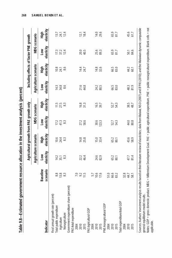
268 SAMUEL BENIN ET AL.Ta
ble 9
.8—Es
timat
ed g
over
nmen
t res
ourc
e allo
catio
n in
the i
nves
tmen
t ana
lysis
(per
cent
)
Ag
ricul
tura
l gro
wth
from
PAE
gro
wth
only
Inclu
ding
effe
cts o
f fas
ter P
NE g
rowt
h
Ag
ricul
ture
scen
ario
MD
G sc
enar
io
Agric
ultu
re sc
enar
io
MDG
scen
ario
Ba
selin
e Lo
w Hi
gh
Low
High
Lo
w Hi
gh
Low
High
Indi
cato
r sc
enar
io
elast
icity
ela
stici
ty
elast
icity
ela
stici
ty
elast
icity
ela
stici
ty
elast
icity
ela
stici
tyRe
al an
nual
grow
th ra
te (p
erce
nt)To
tal pu
blic e
xpen
ditur
e 8.8
14
.2 10
.6 17
.2 11
.5 14
.3 10
.8 17
.3 13
.7
Agric
ultur
e 13
.8 35
.1 24
.4 41
.3 27
.5 34
.8 24
.1 37
.2 24
.1
Nona
gricu
lture
8.3
8.3
8.3
8.3
8.3
8.6
8.6
12
.4 12
.4Go
vern
ment
expe
nditu
re sh
are (
perce
nt)PA
E/tot
al ex
pend
iture
20
04
7.0
2010
9.2
22
.2 14
.8 27
.2 16
.8 21
.6 14
.4 20
.0 12
.1
2015
11
.5 46
.4 25
.8 58
.6 31
.3 44
.8 24
.7 40
.5 18
.4PA
E/ag
ricult
ural
GDP
20
04
5.7
2010
10
.6 24
.6 15
.0 30
.6 16
.5 24
.2 14
.8 25
.6 14
.0
2015
17
.6 82
.9 33
.4 12
3.3
39.7
80.5
32.6
89.3
29.6
PNE/
nona
gricu
ltura
l GDP
20
04
51.0
2010
66
.6 65
.2 65
.2 52
.7 52
.7 66
.5 66
.5 65
.9 65
.9
2015
83
.2 80
.1 80
.1 54
.3 54
.3 83
.0 83
.0 81
.7 81
.7To
tal ex
pend
iture
/total
GDP
20
04
32.8
2010
44
.7 47
.7 43
.6 44
.0 38
.5 48
.3 44
.2 50
.1 45
.6
2015
58
.1 81
.4 58
.9 80
.8 48
.7 81
.9 60
.1 84
.6 61
.7
Sour
ces:
Autho
rs’ in
vestm
ent a
nalys
is re
sults
base
d on t
heir l
itera
ture r
eview
of el
astic
ities;
data
from
Malaw
i, NSO
(200
7) an
d IFP
RI (2
010)
; and
the M
alawi
an dy
nami
c com
putab
le ge
nera
l equ
ilibriu
m mo
del re
sults
.No
tes: G
DP =
gro
ss d
omes
tic p
rodu
ct. M
DG =
Mille
nnium
Dev
elopm
ent G
oal. P
AE =
pub
lic a
gricu
ltura
l exp
endit
ure.
PNE
= pu
blic n
onag
ricult
ural
expe
nditu
re. B
lank c
ells =
not
appli
cable
.
MALAWI 269
When we take the effect of accelerated growth in PNE into account, the share of agricultural spending in total expenditure reaches 24.7–44.8 percent by 2015.
These results confi rm the importance of Malawi’s allocating at least 10 percent of the government’s total budget to agriculture in accordance with the Maputo Declaration on agriculture and food security (AU 2006). In fact, the results suggest that even in a more effi cient spending scenario (that is, high elasticities), the govern-ment will need to allocate at least 25 percent of its total budget to agriculture by 2015 to achieve a 6 percent agricultural growth rate. Considering the 2006–11 period, the total resource envelope proposed in the Malawi Growth and Development Strategy (MGDS) (Malawi, MDPC 2006) seems to be in line with this requirement. However, nearly 51 percent of the total budget is earmarked for the development of the Shire–Zambezi Waterway. It is not clear how much of this money will be spent on the agriculture sector, which includes crops, livestock, forestry, and fi shery. In contrast, direct public spending on agriculture and food security, irrigation and water, and integrated rural development represents only 4.3 percent of the total resource envelope in the MGDS.
The DCGE model results estimate that reaching the 6 percent agricultural growth rate target will signifi cantly improve poverty outcomes. However, even in this accelerated growth scenario, Malawi will not be able to achieve the fi rst MDG. Without complementary accelerated growth in the nonagricultural sectors, the binding demand or market constraints for agricultural outputs will prevent agricul-tural growth from translating into higher household incomes. Halving poverty by 2015 will require a doubling of the growth rate in the nonagricultural sectors (from 3.5 to 7.6 percent) and a higher annual growth rate in agricultural GDP (6.9 per-cent, which is more than double the baseline case of 2.8 percent). Assuming that agricultural growth is driven by growth in PAE only, government spending would have to grow by at least 24.1–37.2 percent annually (assuming a high and low elasticity, respectively) to support such high growth rates. Achieving the fi rst MDG is not only a resource mobilization constraint for the government of Malawi but is also a challenge requiring improved effi ciency of allocating and investing large amounts of resources.
Identifying Investment Priorities Estimating the total public resources needed to reach particular agricultural growth targets is important, but prioritizing investments is equally important. Because of a lack of historical data on specifi c investment programs and related outputs and outcomes, this study is unable to analyze specifi c investment priorities based on their potential agricultural growth and poverty-reduction rates of returns. However, we use results from other studies in an attempt to offer a guide to key investments that could help promote agricultural growth and rural poverty reduction. The evidence
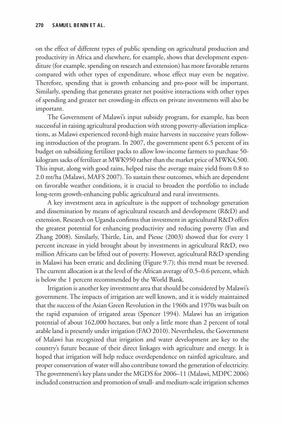
270 SAMUEL BENIN ET AL.
on the effect of different types of public spending on agricultural production and productivity in Africa and elsewhere, for example, shows that development expen-diture (for example, spending on research and extension) has more favorable returns compared with other types of expenditure, whose effect may even be negative. Therefore, spending that is growth enhancing and pro-poor will be important. Similarly, spending that generates greater net positive interactions with other types of spending and greater net crowding-in effects on private investments will also be important.
The Government of Malawi’s input subsidy program, for example, has been successful in raising agricultural production with strong poverty-alleviation implica-tions, as Malawi experienced record-high maize harvests in successive years follow-ing introduction of the program. In 2007, the government spent 6.5 percent of its budget on subsidizing fertilizer packs to allow low-income farmers to purchase 50- kilogram sacks of fertilizer at MWK950 rather than the market price of MWK4,500. This input, along with good rains, helped raise the average maize yield from 0.8 to 2.0 mt/ha (Malawi, MAFS 2007). To sustain these outcomes, which are dependent on favorable weather conditions, it is crucial to broaden the portfolio to include long-term growth-enhancing public agricultural and rural investments.
A key investment area in agriculture is the support of technology generation and dissemination by means of agricultural research and development (R&D) and extension. Research on Uganda confi rms that investment in agricultural R&D offers the greatest potential for enhancing productivity and reducing poverty (Fan and Zhang 2008). Similarly, Thirtle, Lin, and Piesse (2003) showed that for every 1 percent increase in yield brought about by investments in agricultural R&D, two million Africans can be lifted out of poverty. However, agricultural R&D spending in Malawi has been erratic and declining (Figure 9.7); this trend must be reversed. The current allocation is at the level of the African average of 0.5–0.6 percent, which is below the 1 percent recommended by the World Bank.
Irrigation is another key investment area that should be considered by Malawi’s government. The impacts of irrigation are well known, and it is widely maintained that the success of the Asian Green Revolution in the 1960s and 1970s was built on the rapid expansion of irrigated areas (Spencer 1994). Malawi has an irrigation potential of about 162,000 hectares, but only a little more than 2 percent of total arable land is presently under irrigation (FAO 2010). Nevertheless, the Government of Malawi has recognized that irrigation and water development are key to the country’s future because of their direct linkages with agriculture and energy. It is hoped that irrigation will help reduce overdependence on rainfed agriculture, and proper conservation of water will also contribute toward the generation of electricity. The government’s key plans under the MGDS for 2006–11 (Malawi, MDPC 2006) included construction and promotion of small- and medium-scale irrigation schemes
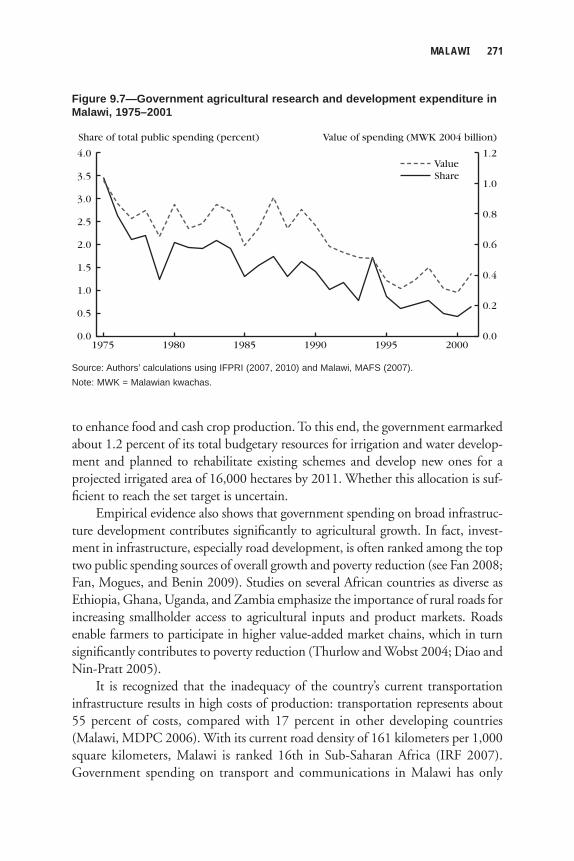
MALAWI 271
to enhance food and cash crop production. To this end, the government earmarked about 1.2 percent of its total budgetary resources for irrigation and water develop-ment and planned to rehabilitate existing schemes and develop new ones for a projected irrigated area of 16,000 hectares by 2011. Whether this allocation is suf-fi cient to reach the set target is uncertain.
Empirical evidence also shows that government spending on broad infrastruc-ture development contributes signifi cantly to agricultural growth. In fact, invest-ment in infrastructure, especially road development, is often ranked among the top two public spending sources of overall growth and poverty reduction (see Fan 2008; Fan, Mogues, and Benin 2009). Studies on several African countries as diverse as Ethiopia, Ghana, Uganda, and Zambia emphasize the importance of rural roads for increasing smallholder access to agricultural inputs and product markets. Roads enable farmers to participate in higher value-added market chains, which in turn signifi cantly contributes to poverty reduction (Thurlow and Wobst 2004; Diao and Nin-Pratt 2005).
It is recognized that the inadequacy of the country’s current transportation infrastructure results in high costs of production: transportation represents about 55 percent of costs, compared with 17 percent in other developing countries (Malawi, MDPC 2006). With its current road density of 161 kilometers per 1,000 square kilometers, Malawi is ranked 16th in Sub-Saharan Africa (IRF 2007). Government spending on transport and communications in Malawi has only
Share of total public spending (percent) Value of spending (MWK 2004 billion)
4.0
0.0
3.5
3.0
2.5
ShareValue
200019951990198519801975
2.0
1.5
1.0
0.5
1.2
0.0
1.0
0.8
0.6
0.4
0.2
Figure 9.7—Government agricultural research and development expenditure in Malawi, 1975–2001
Source: Authors’ calculations using IFPRI (2007, 2010) and Malawi, MAFS (2007).Note: MWK = Malawian kwachas.
272 SAMUEL BENIN ET AL.
recently started to improve, following a decline in the late 1990s (Figure 9.8). Investments in rural feeder roads, in particular, can have large poverty-reduction effects per unit of investment, as Fan and Zhang (2008) show in the case of Uganda. In Uganda, the marginal return to public spending on feeder roads, measured by the increase in poverty reduction and agricultural output, is three to four times larger than the return to public spending on murram and tarmac roads. Under the MGDS, the Malawian government planned to spend MWK7.6 billion during 2006–11 to improve the road network through including routine and periodic maintenance and rehabilitation, among other measures. Although this amount is unlikely to substan-tially improve road density, road conditions will probably improve, with a target of 71 percent of the road network being in good condition, 18 percent in fair condi-tion, and only 11 percent in poor condition.
ConclusionsMalawi has the potential to improve crop yields and shift to an intensifi cation-based growth strategy in its agricultural sector. Reaching and sustaining an annual agri-cultural growth rate of 6 percent requires yield improvements that are well below the potentials identifi ed through fi eld trials. Faster agricultural growth would stimu-late growth outside agriculture, and it would reduce Malawi’s poverty headcount rate to 34.5 percent by 2015. Most households are expected to benefi t, although
Share of total public spending (percent) Value of public spending (MWK 2004 billion)
100
0
90
80
70
200519951990198519801975
60
50
40
30
20
0
15
10
520
10
2000
ShareValue
Figure 9.8—Government transport and communications expenditure in Malawi, 1975–2007
Source: Authors’ calculations using IFPRI (2010) and Malawi, NSO (2007).Note: MWK = Malawian kwachas.
MALAWI 273
some households in regions growing high-value export-oriented crops, such as tobacco and cotton, would stand to gain more than would households in other parts of the country. Moreover, poverty among households in the southern regions would remain high, even with faster agricultural growth. Finally, rural households will benefi t more than urban households, mainly because of their greater dependence on farm incomes. However, urban households should still benefi t, because urban agriculturalists farm 6 percent of agricultural land in Malawi, and agricultural com-modities are an important part of urban consumption baskets.
We used the detailed structure of the Malawian DCGE model to compare the effectiveness of growth driven by different subsectors in reducing poverty and encouraging broader-based growth. Our results indicate that additional growth driven by maize, pulses, and horticultural crops will have larger impacts on poverty reduction than similar growth led by growth in export-oriented crops. This is because yield improvements in the fi rst three crops will not only directly benefi t households by increasing incomes from agricultural production, but also indirectly benefi t them by allowing farmers to diversify their land allocations to include higher value crops. Foodcrops and fi sheries also have strong growth linkages to nonagricultural sectors, thereby stimulating broader economywide growth and poverty reduction. However, the higher growth potential of export crops relative to that of the nonmaize foodcrops means that export-led growth can still account for a signifi cant share of overall poverty reduction. However, the small initial size and geographic concentration of certain crops, such as tea and sugarcane, means that their potential contributions to national growth and poverty reduction will remain limited, at least over the near term. Taken together, the characteristics of the various subsectors highlight the importance of broader-based agricultural growth but sug-gest that priority should be given to maize, pulses, horticulture, and smallholder export crops, such as tobacco and cotton.
Increasing agricultural growth to accelerate agricultural development in Malawi will require both additional investment in the sector and improvements in the effi -ciency of public spending. The investment analysis indicates that government spending on agriculture would have to grow by at least 20 percent per year to achieve and sustain an annual agricultural growth rate of 6 percent. Thus, the government will need to allocate almost one-quarter of its budget to agriculture by 2015. How-ever, this spending scenario assumes that the government is able to invest with an effi ciency exceeding that of many Sub-Saharan African countries. If this condition does not hold, then public spending on agriculture would have to grow at a much higher rate to reach the growth target.
Malawi may have turned the corner on its food and agricultural crises of the early 2000s. Maize production and food security have been greatly improved fol-lowing the introduction of the new input subsidy program. This improvement
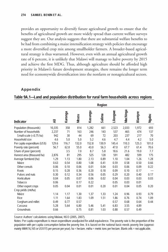
274 SAMUEL BENIN ET AL.
provides an opportunity to diversify future agricultural growth to ensure that the benefi ts of agricultural growth are more widely spread than current welfare surveys suggest they are. Our analysis suggests that there are substantial welfare benefi ts to be had from combining a maize intensifi cation strategy with policies that encourage a more diversifi ed crop mix among smallholder farmers. A broader-based agricul-tural strategy is thus warranted. However, even with an annual agricultural growth rate of 6 percent, it is unlikely that Malawi will manage to halve poverty by 2015 and achieve the fi rst MDG. Thus, although agriculture should be afforded high priority in Malawi’s future development strategies, there remains the longer term need for economywide diversifi cation into the nonfarm or nonagricultural sectors.
Appendix
Table 9A.1—Land and population distribution for rural farm households across regions
Region
Indicator Population (thousands) 10,335 358 814 1,282 661 2,523 2,033 1,972 693Number of households 2,237 71 163 246 143 537 465 474 137 Small-scale (<0.75 ha) 942 30 44 69 72 203 237 217 70Household size 4.6 5.0 5.0 5.2 4.6 4.7 4.4 4.2 5.0 Per capita expenditure (US$) 129.6 116.7 132.0 152.8 130.9 145.4 110.3 125.3 101.0Poverty rate (percent) 56.7 62.8 55.0 43.0 56.3 47.0 67.7 61.4 70.6Share of poor (percent) 3.5 7.0 8.7 5.8 18.6 21.6 19.0 7.7Harvest area (thousand ha) 2,876 81 295 525 128 591 482 599 175Average farmland (ha) 1.29 1.13 1.80 2.13 0.89 1.10 1.04 1.26 1.28 Maize 0.63 0.54 0.80 1.08 0.41 0.59 0.58 0.50 0.66 Other cereals 0.06 0.10 0.06 0.01 0.04 0.03 0.06 0.09 0.22 Roots 0.15 0.28 0.36 0.20 0.18 0.09 0.10 0.17 — Pulses and nuts 0.30 0.12 0.34 0.56 0.05 0.29 0.20 0.40 0.17 Horticulture 0.04 0.05 0.07 0.06 0.02 0.04 0.03 0.03 0.03 Tobacco 0.06 0.17 0.22 0.05 0.03 0.01 Other export crops 0.05 0.04 0.01 0.01 0.20 0.01 0.04 0.05 0.20Crop yields (mt/ha) Maize 1.14 1.17 1.30 1.37 1.33 1.24 0.96 0.93 0.79 Rice 1.11 1.64 1.83 1.09 1.51 1.86 0.76 0.74 1.09 Sorghum and millet 0.49 0.77 0.57 0.57 0.68 0.64 0.44 Cassava 5.28 5.64 6.80 5.46 5.41 6.83 3.55 4.89 Groundnuts 0.66 0.75 0.81 1.03 0.88 0.57 0.49
Source: Authors’ calculations using Malawi, NSO (2005, 2007).Notes: Per capita expenditure is mean expenditure unadjusted for adult equivalence. The poverty rate is the proportion of the population with per capita consumption below the poverty line. It is based on the national basic-needs poverty line (approxi-mately MWK16,165 or US$115 per person per year). ha = hectare. mt/ha = metric tons per hectare. Blank cells = not applicable.
All
Karo
nga
Mzuz
u
Kasu
ngu
Salim
a
Lilo
ngwe
Mach
inga
Blan
tyre
Ngab
u
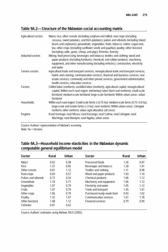
MALAWI 275
Table 9A.2— Structure of the Malawian social accounting matrix
Agricultural sectors Maize; rice; other cereals (including sorghum and millet); root crops (including cassava, sweet potatoes, and Irish potatoes); pulses and oilseeds (including mixed
beans and soybeans); groundnuts; vegetables; fruits; tobacco; cotton; sugarcane; tea; other crops (including sunflower seeds and paprika); poultry; other livestock (including cattle, goats, sheep, and pigs); fisheries; forestry
Industrial sectors Mining; food processing; beverages and tobacco; textiles and clothing; wood and paper products (including furniture); chemicals and rubber products; machinery,
equipment, and other manufacturing (including vehicles); construction; electricity and water
Service sectors Agricultural trade and transport services; nonagricultural trade and transport services; hotels and catering; communication services; financial and business services; real
estate services; community and other private services; government administration; health services; education services
Factors Skilled labor (nonfarm); unskilled labor (nonfarm); agricultural capital; nonagricultural capital; Within each rural region: elementary labor (farm and nonfarm); small-scale
farmland; medium-scale farmland; large-scale farmland; Within urban areas: urban farmland
Households Within each rural region: Small-scale farms (<0.75 ha); medium-scale farms (0.75–3.0 ha); large-scale and estate farms (>3 ha); rural nonfarm; Within urban areas: Lilongwe
nonfarm; other nonfarm; urban agriculturalists (all sizes)Regions Rural Karonga; rural Mzuzu; rural Kasungu; rural Salima; rural Lilongwe; rural Machinga; rural Blantyre; rural Ngabu; urban areas
Source: Authors’ representation of Malawi’s economy.Note: ha = hectare.
Table 9A.3—Household income elasticities in the Malawian dynamic computable general equilibrium model
Sector Rural Urban Sector Rural UrbanMaize 0.62 0.38 Processed foods 1.26 0.87Rice 1.37 0.85 Beverages and tobacco 1.28 1.01Other cereals 0.81 1.12 Textiles and clothing 1.11 0.98Root crops 0.69 0.57 Wood and paper products 1.03 1.16Pulses and oilseeds 0.72 0.54 Chemical products 1.06 1.12Groundnuts 1.18 0.71 Machinery and equipment 1.06 1.12Vegetables 1.07 0.79 Electricity and water 1.05 1.12Fruits 1.07 0.79 Trade and transport 1.45 1.61Other crops 1.06 0.79 Purchased ready-made food 0.93 1.02Poultry 1.32 1.07 Communication services 1.61 1.78Other livestock 1.48 1.12 Financial services 0.79 0.99Fisheries 0.81 0.62
Source: Authors’ estimates using Malawi, NSO (2005).
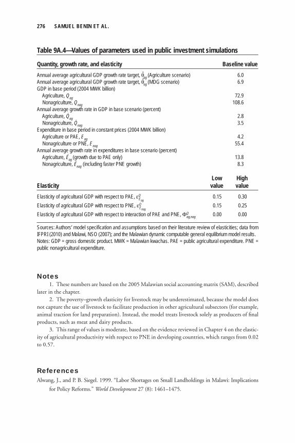
276 SAMUEL BENIN ET AL.
Table 9A.4—Values of parameters used in public investment simulations
Quantity, growth rate, and elasticity Baseline valueAnnual average agricultural GDP growth rate target, θag (Agriculture scenario) 6.0Annual average agricultural GDP growth rate target, θag (MDG scenario) 6.9GDP in base period (2004 MWK billion) Agriculture, Qag 72.9 Nonagriculture, Qnag 108.6Annual average growth rate in GDP in base scenario (percent) Agriculture, Qag 2.8 Nonagriculture, Qnag 3.5Expenditure in base period in constant prices (2004 MWK billion) Agriculture or PAE, Eag 4.2 Nonagriculture or PNE, Enag 55.4Annual average growth rate in expenditures in base scenario (percent) Agriculture, Eag (growth due to PAE only) 13.8 Nonagriculture, Enag (including faster PNE growth) 8.3
Low HighElasticity value valueElasticity of agricultural GDP with respect to PAE, εQ
Eag 0.15 0.30
Elasticity of agricultural GDP with respect to PNE, εQEnag
0.15 0.25Elasticity of agricultural GDP with respect to interaction of PAE and PNE, ΦQ
ag,nag 0.00 0.00
Sources: Authors’ model specification and assumptions based on their literature review of elasticities; data from IFPRI (2010) and Malawi, NSO (2007); and the Malawian dynamic computable general equilibrium model results.Notes: GDP = gross domestic product. MWK = Malawian kwachas. PAE = public agricultural expenditure. PNE = public nonagricultural expenditure.
Notes 1. These numbers are based on the 2005 Malawian social accounting matrix (SAM), described later in the chapter. 2. The poverty–growth elasticity for livestock may be underestimated, because the model does not capture the use of livestock to facilitate production in other agricultural subsectors (for example, animal traction for land preparation). Instead, the model treats livestock solely as producers of fi nal products, such as meat and dairy products. 3. This range of values is moderate, based on the evidence reviewed in Chapter 4 on the elastic-ity of agricultural productivity with respect to PNE in developing countries, which ranges from 0.02 to 0.57.
ReferencesAlwang, J., and P. B. Siegel. 1999. “Labor Shortages on Small Landholdings in Malawi: Implications
for Policy Reforms.” World Development 27 (8): 1461–1475.
MALAWI 277
AU (African Union). 2006. Ten Percent Budget Allocation to Agriculture and Rural Development: Next
Steps. Addis Ababa, Ethiopia.
Benin, S., T. Mogues, G. Cudjoe, and J. Randriamamonjy. 2008. Reaching Middle-Income Status in
Ghana by 2015: Public Expenditures and Agricultural Growth. Discussion Paper 811. Washington,
DC: International Food Policy Research Institute.
Carr, S. J. 1997. “A Green Revolution Frustrated: Lessons from the Malawi Experience.” African Crop
Science Journal 5 (1): 93–98.
Chilowa, W. 1998. “The Impact of Agricultural Liberalization on Food Security in Malawi.” Food Policy
23 (6): 553–569.
Chulu, O., and P. Wobst. 2001. A 1998 Social Accounting Matrix for Malawi. Trade and Macro-
economics Discussion Paper 69. Washington, DC: International Food Policy Research Institute.
Diagne, A., and M. Zeller. 2001. Access to Credit and Its Impact on Welfare in Malawi. Research Report
116. Washington, DC: International Food Policy Research Institute.
Diao, X., and A. Nin-Pratt. 2005. Growth Options and Poverty Reduction in Ethiopia: A Spatial,
Economywide Model Analysis for 2004–2015. Development Strategy and Governance Division
Discussion Paper 20. Washington, DC: International Food Policy Research Institute.
Diao, X., P. Hazell, D. Resnick, and J. Thurlow. 2007. The Role of Agriculture in Pro-Poor Growth in
Sub-Saharan Africa. Research Report 144. Washington, DC: International Food Policy Research
Institute.
Dorward, A. 2006. “Markets and Pro-Poor Agricultural Growth: Insights from Livelihood and Informal
Rural Economy Models in Malawi.” Agricultural Economics 35 (2): 157–169.
Dorward, A., and E. Chirwa. 2011. “The Malawi Agricultural Input Subsidy Programme: 2005–6 to
2008–9.” International Journal of Agricultural Sustainability 9 (1): 232–247.
Dorward, A., and J. Kydd. 2004. “The Malawi 2002 Food Crisis: The Rural Development Challenge.”
Journal of Modern African Studies 42 (3): 343–361.
Fafchamps, M., E. Gabre-Madhin, and B. Minten. 2005. “Increasing Returns and Market Effi ciency
in Agricultural Trade.” Journal of Development Economics 78: 406–442.
Fan, S., ed. 2008. Public Expenditures, Growth, and Poverty: Lessons from Developing Countries. Baltimore:
Johns Hopkins University Press.
Fan, S., and X. Zhang. 2004. “Investment, Reforms and Poverty in Rural China.” Economic Development
and Cultural Change 52 (2): 395–422.
———. 2008. “Public Expenditure, Growth, and Poverty Reduction in Rural Uganda.” African
Development Review 20 (3): 466–496.
Fan, S., T. Mogues, and S. Benin. 2009. Setting Priorities for Public Spending for Agricultural and Rural
Development in Africa. Policy Brief 12. Washington, DC: International Food Policy Research
Institute.
278 SAMUEL BENIN ET AL.
Fan, S., B. Yu, and A. Saurkar. 2008. “Public Spending in Developing Countries: Trends, Determination,
and Impact.” In Public Expenditures, Growth, and Poverty: Lessons from Developing Countries,
edited by S. Fan, 20–25. Baltimore: Johns Hopkins University Press.
FAO (Food and Agriculture Organization of the United Nations). 2010. FAOSTAT Statistical Database.
Accessed September 16, 2011. http://faostat.fao.org/.
Harrigan, J. 2003. “U-Turns and Full Circles: Two Decades of Agricultural Reform in Malawi,
1981–2000.” World Development 31 (5): 847–863.
———. 2008. “Food Insecurity, Poverty and the Malawian Starter Pack: Fresh Start or False Start?”
Food Policy 33: 237–249.
IFPRI (International Food Policy Research Institute). 2007. “Agricultural Science and Technology
Indicators.” Accessed December 15. www.asti.cgiar.org/.
———. 2010. “Statistics on Public Expenditure for Economic Development (SPEED).” Accessed
January 12. www.ifpri.org/book-39/ourwork/programs/priorities-public-investment/speed-data
base.
IRF (International Road Federation). 2007. World Road Statistics. Geneva.
Kherallah, M., and K. Govindan. 1999. “The Sequencing of Agricultural Market Reforms in Malawi.”
Journal of African Economies 8 (2): 125–151.
Malawi, MAFS (Ministry of Agriculture and Food Security). 2003. Crop Budgets. Lilongwe, Malawi:
Agricultural Research and Extension Trust, Ministry of Agriculture and Food Security.
———. 2007. District Agricultural Production Series. Lilongwe, Malawi.
Malawi, MDPC (Ministry of Development Planning and Cooperatives). 2006. Malawi Growth and
Development Strategy. Lilongwe, Malawi.
Malawi, NSO (National Statistical Offi ce). 2005. Malawi Second Integrated Household Survey (IHS2)
2004–05. Lilongwe, Malawi.
———. 2007. Statistical Yearbook. Lilongwe, Malawi.
———. 2009. Malawi Welfare Monitoring Survey. Lilongwe, Malawi.
Orr, A. 2000. “‘Green Gold?’: Burley Tobacco, Smallholder Agriculture, and Poverty Alleviation in
Malawi.” World Development 28 (2): 347–363.
Orr, A., and B. Mwale. 2001. “Adapting to Adjustment: Smallholder Livelihood Strategies in Southern
Malawi.” World Development 29 (8): 1325–1343.
Pauw, K., J. Thurlow, M. Bachu, and D. E. van Seventer. 2010. “The Economic Costs of Extreme
Weather Events: A Hydro-Meteorological CGE Analysis for Malawi.” Environment and Development
Economics. DOI: 10.1017/S1355770X10000471.
Sanchez, P. A., G. L. Denning, and G. Nziguheb. 2009. “The African Green Revolution Moves
Forward.” Food Security 1: 37–44.

MALAWI 279
Spencer, D. 1994. Infrastructure and Technology Constraints to Agricultural Development in the Humid
and Subhumid Tropics of Africa. Environment and Production Technology Division Discussion
Paper 3. Washington, DC: International Food Policy Research Institute.
Thirtle, C., L. Lin, and J. Piesse. 2003. “The Impact of Research-Led Agricultural Productivity Growth
on Poverty Reduction in Africa, Asia and Latin America.” World Development 31 (12):
1959–1975.
Thurlow, J., and P. Wobst. 2004. “Not All Growth Is Equally Good for the Poor: The Case of Zambia.”
Journal of African Economies 15 (4): 603–625.
World Bank. 2010. World Development Indicators. Washington, DC.

C h a p t e r 1 0
UgandaSamuel Benin, James Thurlow, Xinshen Diao,
Allen Kebba, and Nelson Ofwono
Uganda is often heralded as an African success story. The country re-established political stability after the civil wars following Idi Amin’s overthrow and subsequently experienced strong economic growth during the 1990s. Gross
domestic product (GDP) grew rapidly at almost 4 percent annually in per capita terms during 1993–2000 (Uganda, BOS 2008a). At least part of this rapid growth was due to a program of economic reforms, although the implications of these reforms were not universally positive (see, for example, Dijkstra and Van Donge 2001). Economic growth during the 1990s was also broadly based, with per capita agricultural GDP rising by about 1.5 percent per year, driven by both food and traditional export crops. Economywide growth greatly reduced poverty in both rural and urban areas (Uganda, BOS 2008b). Moreover, poverty rates fell fast enough to offset high population growth, and by 2000 there were almost three million fewer people living below the poverty line than in 1993. Agricultural growth thus played a key role during Uganda’s successful recovery period by fostering broad-based growth and poverty reduction (Kappel, Lay, and Steiner 2005).
After 2000 there was a signifi cant shift in the level and composition of growth. Per capita GDP growth slowed to a little more than 2 percent per year, driven almost entirely by a decline in agricultural production. Traditional export crops like coffee were especially hurt by falling world prices (Bussolo et al. 2006). However, it was falling foodcrop production that really undermined agricultural GDP—a situation that improved only marginally during 2007–09 (Uganda, BOS 2010). Thus, although the recovery of the 1990s was broadly based, so too was the subsequent slowdown in economic growth. This slowdown caused a sharp deceleration in the rate of poverty reduction during 2000–06 and an increase in rural–urban migration.
282 SAMUEL BENIN ET AL.
Population growth exceeded poverty reduction between 2000 and 2006, and the number of poor people increased by almost a million. Moreover, Uganda’s poverty–growth elasticity fell from –1.8 during 1993–2006 to –0.6 during 2000–06 (see Table 10A.1 in the appendix to this chapter). Thus, not only did the level of eco-nomic growth decline after 2000, but the stagnation of agriculture also limited the ability of growth to reduce poverty.
The post-2000 slowdown marked the end of Uganda’s postconfl ict recovery period and the onset of a more challenging period for structural transformation (see Bahiigwa, Rigby, and Woodhouse 2005). Agricultural productivity has stagnated in recent years, particularly for foodcrops, and the fueling of agricultural growth through land expansion is increasingly unsustainable. However, low productivity does not refl ect poor agroclimatic conditions or a lack of growth potential. Rather, it is a consequence of underinvestment in the agricultural sector (Benin et al. 2007; Fan and Zhang 2008). Empirical studies of Uganda confi rm that a range of policy options exists that can signifi cantly enhance agricultural productivity, including rural education (Appleton and Balihuta 1996), rural infrastructure and market access (Canagarajah, Newman, and Bhattamishra 2001; Fan and Zhang 2008), agricultural research and extension (Fan and Zhang 2008), land management prac-tices (Pender 2004; Pender et al. 2004), and crop and livestock disease control (see, for example, Baffes 2006).
The need to improve agricultural policies and investment more heavily in the sector is recognized by Uganda’s government. The country has in place two strategies to accelerate agricultural growth, including the Plan for the Modernisation of Agriculture (PMA) and the president’s Prosperity for All initiative (Uganda, MFPED 2008). Moreover, the government has committed itself to the Comprehensive Africa Agriculture Development Programme (CAADP), which is an Africa-wide initiative of the New Partnership for Africa’s Development (NEPAD). A key element of CAADP is a commitment to increase agricultural growth to 6 percent per year by allocating at least 10 percent of the budget to the agricultural sector. These targets present an ambitious but unavoidable challenge for Uganda as it seeks to re-establish the pro-poor growth achieved during the 1990s.
In this chapter we evaluate the potential contribution of alternative agricultural growth paths in generating broadly based economic growth and poverty reduction in Uganda. More specifi cally, we examine the opportunities and constraints to meet-ing the CAADP 6 percent agricultural growth target. We also estimate the cost of public investments needed to accelerate agricultural growth. To this end, we develop a recursive dynamic computable general equilibrium (DCGE) model of Uganda based on the one described in Chapter 2 of this volume. The model integrates a simple farm-modeling approach into the DCGE based on a detailed survey-based farm typology.
UGANDA 283
The chapter is structured as follows. We fi rst review the structure of Uganda’s agricultural sector as refl ected in the farm typology. We then describe the structure of the Ugandan DCGE model and the data used to calibrate it. The simulation results are then discussed for the baseline growth scenario and various accelerated agricultural growth scenarios. This is followed by an investment cost analysis. We conclude the chapter by summarizing our fi ndings.
Agriculture in UgandaTo construct a typology of the farmers making up Uganda’s agricultural sector, we fi rst disaggregate agricultural production across rural and urban areas. Information on crop production was drawn from the 2005/06 Uganda National Household Survey (UNHS3) (Uganda, BOS 2008a), which asked households how much of their agricultural land was devoted to different crops. It also asked households about their cattle assets. The farm typology is based on these cropping patterns and live-stock endowments. The aim of the typology is to group farmers into major catego-ries based on their agricultural activities, which mainly refl ect agroecological, technological, and marketing conditions. These initial conditions will be important in determining the distributional and poverty implications of growth in different agricultural subsectors.
According to the survey, 3.61 million rural households reported agricultural crop incomes in 2005/06. This number is shown in the leftmost box of Figure 10.1, which illustrates the general structure of the farm typology for all rural households engaged in crop production. At this stage we exclude urban agriculturalists and nonfarm households. We fi rst separate out farm households that reported produc-ing high-value export-oriented crops, such as coffee, cotton, tobacco, and tea. In 2005/06, 1.59 million farm households produced these export crops—almost half of all rural farm households in Uganda.
Figure 10.1 shows that coffee is the dominant export crop, with 1.13 million households allocating land to coffee production. We then further split farm house-holds according to whether they produced maize. Although matoke is the key staple foodcrop for most farmers, it is less effective than maize as a means of distinguishing farm types. This can be seen in Table 10.1, which presents summary statistics for the various farm types.
The table shows that, even though coffee farmers generally have larger than average farm plots, farmers growing both coffee and maize (farm groups T1–2) tend to have larger plots than coffee farmers without maize (T3–4) (2.69 hectares com-pared to 1.86 hectares). However, coffee farmers typically allocate similar amounts of land to matoke (about 0.8 hectares), regardless of whether they grow maize. This tendency is equally true of other farm types. More importantly, coffee and maize
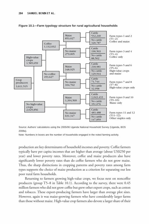
284 SAMUEL BENIN ET AL.
production are key determinants of household incomes and poverty. Coffee farmers typically have per capita incomes that are higher than average (about US$250 per year) and lower poverty rates. Moreover, coffee and maize producers also have signifi cantly lower poverty rates than do coffee farmers who do not grow maize. Thus, the sharp distinctions in cropping patterns and poverty rates among farm types supports the choice of maize production as a criterion for separating out less poor rural farm households.
Returning to farmers growing high-value crops, we focus next on noncoffee producers (group T5–8 in Table 10.1). According to the survey, there were 0.45 million farmers who did not grow coffee but grew other export crops, such as cotton and tobacco. These export-producing farmers have larger than average plot sizes. However, again it was maize-growing farmers who have considerably larger farms than those without maize. High-value crop farmers also devote a larger share of their
Cattle532,240
No cattle320,787Coffee
1,132,032
Maize853,027
No maize279,005
No coffee453,627
Maize1,394,509
Maize348,925
No maize104,702
No high-valuecrops2,025,856
No maize631,347
Cropproducers 3,611,515
Farm types 11 and 12(T11–12):Other staples only
Farm types 9 and 10(T9–10):Maize only
Farm types 7 and 8(T7–8):High-value crops only
Farm types 5 and 6(T5–6):High-value cropsand maize
Farm types 3 and 4(T3–4):Coffee only
Farm types 1 and 2(T1–2):Coffee and maize
High-valuecrops1,585,659
Cattle190,503
No cattle88,502
Cattle218,981
No cattle129,944
Cattle71,744
No cattle32,958
Cattle1,043,433
No cattle351,076
Cattle483,488
No cattle147,859
Figure 10.1—Farm typology structure for rural agricultural households
Source: Authors’ calculations using the 2005/06 Uganda National Household Survey (Uganda, BOS 2008a).Note: Numbers in boxes are the number of households engaged in the noted farming activity.
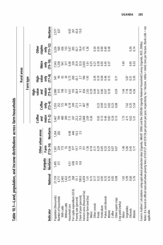
UGANDA 285Ta
ble 1
0.1—
Land
, pop
ulat
ion,
and
inco
me d
istrib
utio
ns ac
ross
farm
hou
seho
lds
Ru
ral a
reas
Fa
rm ty
pe
Hi
gh-
Co
ffee
va
lue
High
-
Othe
r
and
Co
ffee
and
valu
e Ma
ize
stap
les
Farm
maiz
e on
ly
maiz
e on
ly on
ly on
lyIn
dica
tor
Natio
nal
Nonf
arm
(T
13–1
4)
Nonf
arm
(T
1–2)
(T
3–4)
(T
5–6)
(T
7–8)
(T
9–10
) (T
11–1
2)
Nonf
arm
Popu
lation
(tho
usan
ds)
27,15
9 1,4
05
1,501
1,2
64
5,467
1,5
55
2,080
54
1 7,5
43
3,226
2,5
77Nu
mber
of ho
useh
olds
4,717
31
1 22
9 28
2 76
9 25
2 31
5 94
1,2
58
569
637
W
ith ca
ttle
2,465
173
48
0 17
2 19
8 65
94
1 43
6
With
out c
attle
1,022
55
28
9 80
11
7 30
31
7 13
3 Ho
useh
old si
ze
5.76
4.51
6.56
4.48
7.11
6.18
6.61
5.73
6.00
5.67
4.05
Per c
apita
expe
nditu
re (U
S$)
268
638
377
440
247
249
193
200
220
205
261
Pove
rty ra
te (p
erce
nt)
31.1
4.9
19.7
16.5
23.2
27.5
36.9
42.1
35.9
43.1
42.6
Shar
e of p
oor (
perce
nt)
100.0
0.8
3.5
2.5
15
.0 5.1
9.1
2.7
32
.0 16
.4 13
.0Ha
rvest
area
(tho
usan
d ha)
6,6
59
31
1
2,068
46
7 83
4 18
4 2,0
20
775
Aver
age f
arm
land (
ha)
1.41
1.3
6
2.69
1.86
2.65
1.95
1.61
1.36
Ma
ize
0.15
0.1
8
0.36
0.2
9
0.25
Othe
r cer
eals
0.17
0.1
1
0.44
0.39
0.21
0.34
Ro
ots
0.22
0.2
9
0.42
0.23
0.41
0.19
0.28
0.20
Ho
rticult
ure
0.05
0.0
5
0.13
0.09
0.06
0.04
0.05
0.00
Pu
lses a
nd oi
lseed
s 0.3
3
0.33
0.4
6 0.3
1 0.6
7 0.4
6 0.4
5 0.4
0
Mat
oke
0.35
0.2
5
0.82
0.83
0.18
0.15
0.37
0.38
Co
ffee
0.05
0.0
7
0.24
0.23
Ot
her e
xpor
t cro
ps
0.08
0.0
7
0.13
0.08
0.59
0.71
Crop
yield
(mt/h
a)
Ma
ize
1.65
1.4
0
1.73
1.4
4
1.69
Vege
tables
5.9
9
5.06
4.1
1 7.6
2 7.1
8 5.8
7
Oilse
eds
0.60
0.4
5
0.62
0.35
0.38
0.31
0.95
0.30
M
atok
e 5.7
6
5.11
5.3
1 5.5
4 4.5
6 5.4
5 6.5
3 6.1
4
Sour
ce: A
uthor
s’ ca
lculat
ions u
sing a
gricu
ltura
l pro
ducti
on da
ta (U
gand
a, MA
AIF
2006
) and
the 2
005/0
6 Uga
nda N
ation
al Ho
useh
old S
urve
y (Ug
anda
, BOS
2008
a).
Notes
: It is
base
d on o
fficial
rura
l and
urba
n pov
erty
lines
of U
S$12
1 and
US$
136 p
er pe
rson p
er ye
ar, re
spec
tively
. ha =
hecta
re. m
t/ha =
metr
ic ton
s per
hecta
re. B
lank c
ells =
not
appli
cable
.
Othe
r urb
an ar
eas
Kam
pala
286 SAMUEL BENIN ET AL.
land to nonmaize cereals, such as sorghum and millet, and to pulses and oilseeds. Accordingly, their land allocations to matoke are lower than that of coffee farmers. Poverty rates are higher among high-value farmers versus coffee-producing farm-ers, and Table 10.1 shows that high-value farmers growing maize are less likely to be poor than farmers not growing maize. The typology therefore reveals that even though coffee and export-crop farmers have similarly large farms, coffee appears to be a major determinant of poverty among farm households.
Finally, we consider the 2 million farm households in Uganda not engaged in export-crop production. Two-thirds of these farm households grow maize (T9–10), whereas the rest are more reliant on other staple crops, such sorghum, millet, and matoke (T11–12). Plot sizes for nonexport farmers are signifi cantly smaller than those of the other farm types, especially for producers of nonmaize staple crops, whose farms average only 1.36 hectares. Despite having smaller farms, per capita incomes and poverty rates for these farmers are similar to those of staple-oriented and high-value farm types. This fact suggests a greater reliance on nonfarm income sources for staple-oriented households. Again maize-producing households have lower poverty rates than households that rely on other staple crops, although they remain above the average poverty rate for all rural areas. Because of these high pov-erty rates and the large number of these farm types, almost half of Uganda’s poor population falls into one of the nonexport farm household types.
Livestock is an important income source for many households (see Ellis and Bahiigwa 2003). As shown in Table 10.1, about half of Ugandan households and more than two-thirds of Ugandan farm households own cattle. The survey also suggests that livestock ownership is a key determinant of poverty. Table 10.2 shows average per capita expenditures for the various farm types, disaggregated according to whether the households own cattle. Households with cattle have signifi cantly higher per capita expenditures and markedly lower poverty rates (20.7 percent for households with cattle compared to 33.5 percent for those without). This relation-ship between livestock and welfare also exists for individual farm types, with the exception of the “high-value only” group. Thus, over and above the crop-based disaggregation of farm households discussed above, the typology also separates each farm type into two subcategories according to whether the households own cattle.
Figure 10.1 shows only six broad rural farm household types, with two subtypes in each, and does not include the urban households engaged in crop production, which have long been an important part of the agricultural sector (see Maxwell 1995). As seen in Table 10.1, the urban agriculturalist farm type (with includes the two subtypes T11–12) is an important part of the agricultural sector, comprising about 229,000 households and 1.5 million individuals (about 5.5 percent of the total population). Urban farm households tend to be larger than rural households (6.2 individuals per household), although urban plot sizes are smaller than the
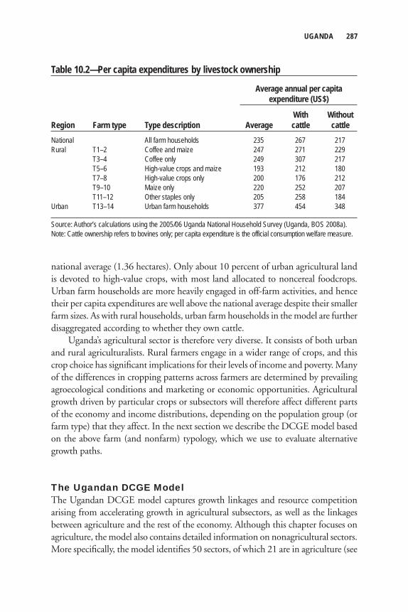
UGANDA 287
national average (1.36 hectares). Only about 10 percent of urban agricultural land is devoted to high-value crops, with most land allocated to noncereal foodcrops. Urban farm households are more heavily engaged in off-farm activities, and hence their per capita expenditures are well above the national average despite their smaller farm sizes. As with rural households, urban farm households in the model are further disaggregated according to whether they own cattle.
Uganda’s agricultural sector is therefore very diverse. It consists of both urban and rural agriculturalists. Rural farmers engage in a wider range of crops, and this crop choice has signifi cant implications for their levels of income and poverty. Many of the differences in cropping patterns across farmers are determined by prevailing agroecological conditions and marketing or economic opportunities. Agricultural growth driven by particular crops or subsectors will therefore affect different parts of the economy and income distributions, depending on the population group (or farm type) that they affect. In the next section we describe the DCGE model based on the above farm (and nonfarm) typology, which we use to evaluate alternative growth paths.
The Ugandan DCGE ModelThe Ugandan DCGE model captures growth linkages and resource competition arising from accelerating growth in agricultural subsectors, as well as the linkages between agriculture and the rest of the economy. Although this chapter focuses on agriculture, the model also contains detailed information on nonagricultural sectors. More specifi cally, the model identifi es 50 sectors, of which 21 are in agriculture (see
Table 10.2—Per capita expenditures by livestock ownership
Average annual per capita expenditure (US$)
With WithoutRegion Farm type Type description Average cattle cattleNational All farm households 235 267 217Rural T1–2 Coffee and maize 247 271 229 T3–4 Coffee only 249 307 217 T5–6 High-value crops and maize 193 212 180 T7–8 High-value crops only 200 176 212 T9–10 Maize only 220 252 207 T11–12 Other staples only 205 258 184Urban T13–14 Urban farm households 377 454 348
Source: Author’s calculations using the 2005/06 Uganda National Household Survey (Uganda, BOS 2008a).Note: Cattle ownership refers to bovines only; per capita expenditure is the official consumption welfare measure.
288 SAMUEL BENIN ET AL.
Table 10A.2 in the appendix to this chapter). Agricultural crops fall into fi ve catego-ries: (1) cereal crops (maize, rice, sorghum, and millet); (2) root crops (cassava, Irish potatoes, and sweet potatoes); (3) horticulture (vegetables and fruits); (4) other food crops (beans, matoke, and pulses and oilseeds); and (5) high-value export-oriented crops (for example, cotton, tobacco, coffee, and sugarcane). The model also identi-fi es other noncrop subsectors, including three livestock subsectors, namely, cattle, poultry, and other livestock (such as sheep, goats, and pigs). Forestry and fi sheries also appear as separate sectors. These agricultural commodities are not only exported and consumed by households, but they are also inputs for downstream processing activities in manufacturing. The eight processing activities in the model include meat, fi sh, grain, animal feed, other food, beverages and tobacco, textiles and clothing, and wood processing. Conversely, agricultural subsectors also use non-agricultural inputs, such as fertilizers from the chemical sector and marketing ser-vices from the trade sectors.
The DCGE model is calibrated to the initial cropping patterns of each of the 14 farm types (which consist of 7 broad farm types, each including two subtypes) described in the previous section. Each group of farmers (represented by the various farm types) responds to changes in production technology, commodity demand, and prices by reallocating their lands across different crops to maximize their incomes. These representative farmers also allocate their labor and capital endow-ments between farm and nonfarm activities, including livestock and fi shing, wage employment on other people’s farms, and migration to nonagriculture in more urbanized sectors. The DCGE model segments labor markets into different catego-ries: self-employed farmworkers, unskilled workers (both on- and off-farm), and skilled nonfarm workers. Information on employment and wages by sector was taken from the household survey UNHS3.
By capturing production information at the farm level, the DCGE model integrates different actors and activities into an economywide model that can assess growth effects at the macrolevel while also taking into account the microlevel decisionmaking typically associated with more detailed farm models. The Ugandan model is therefore an ideal tool for capturing the growth linkages and income and price effects resulting from accelerating growth in different agricultural sectors.
Finally, the Uganda model endogenously estimates the impact of alternative growth paths on the incomes of various household groups. These household groups follow the farm typology by including farm and nonfarm households. In Uganda they are disaggregated across rural areas, the major city of Kampala, and other smaller urban centers. Each household in UNHS3 is linked directly to its corre-sponding representative household in the DCGE model. This linking is the micro-simulation component of the model. In this formulation, changes in representative households’ consumption spending and prices in the DCGE model are passed down
UGANDA 289
to their corresponding households in the survey, where the consumption measures are recalculated. The new level of per capita expenditure for each survey house-hold is compared to the offi cial poverty line, and standard poverty measures are recalculated. Thus, poverty in the model is measured in the same way as offi cial poverty estimates, and changes in poverty refl ect the consumption patterns and in-come distributions from UNHS3.
The data used to calibrate the base year of the model are drawn from a variety of sources. The core dataset underlying the Ugandan model is a 2005 social account-ing matrix that was constructed using information from national accounts, supply–use tables, and balance of payments from the Uganda Bureau of Statistics (see Thurlow, Diao, and Zhu 2007). Agricultural production data were provided by the Ministry of Agriculture, Animal Industries and Fisheries (Uganda, MAAIF 2006), and supplemented by information by the Food and Agriculture Organization (FAO 2010). Agricultural production was fi rst disaggregated across sectors using offi cial production estimates. Production was then disaggregated across farm types using information from UNHS3. Nonagricultural production and employment data are from UNHS3 and national accounts. On the demand side, information on produc-tion technologies (that is, intermediate and factor demands) was taken from the 2002/03 supply–use table (Uganda, BOS 2008c); the income and expenditure pat-terns for the various household groups are from UNHS3.
Baseline Growth ScenarioThe model is fi rst used to examine the impact of Uganda’s current growth path on poverty. This business-as-usual or baseline scenario draws on recent and observed production trends for the various subsectors in the model to construct a growth trajectory for 2005–15. Despite the slowdown in economic growth since the 1990s, Uganda has still performed relatively well, with national GDP growing at around 5 percent per year. However, as mentioned earlier, the agricultural sector has experi-enced far more modest growth. Agricultural growth has also been erratic, with agricultural GDP rising during 2002–03, falling in 2004, and then remaining stagnant during 2005–06. In the baseline, we assume that agricultural GDP will perform closer to what was observed during 2006–09, growing at 2.7 percent per year during 2005–15. Moreover, most agricultural production growth since 1990 has been due to area expansion, with average weighted yields falling over this period (FAO 2010). In the baseline, we assume that land expansion will continue, but at a more modest pace, with only two-thirds of production growth driven by area expansion. This rate is equivalent to a 2 percent increase in harvested land per year during 2005–15 and is lower than the rural population growth rate of 3.2 percent. As shown in Table 10.3, the nonagricultural sectors are assumed to maintain their
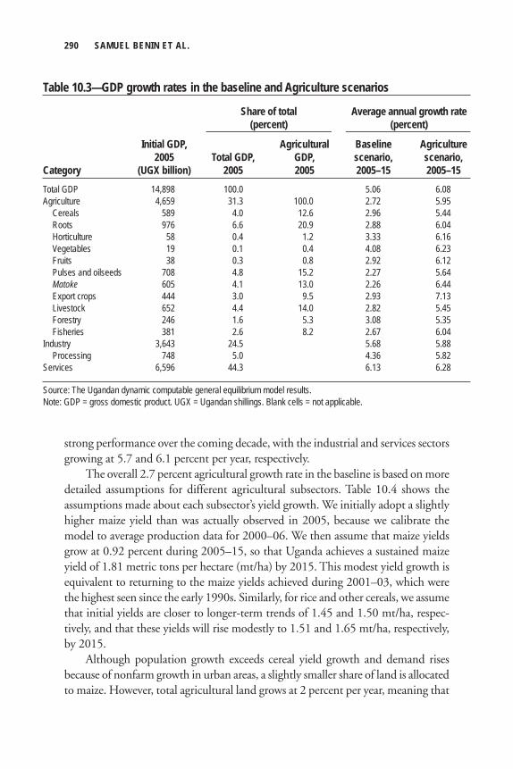
290 SAMUEL BENIN ET AL.
strong performance over the coming decade, with the industrial and services sectors growing at 5.7 and 6.1 percent per year, respectively.
The overall 2.7 percent agricultural growth rate in the baseline is based on more detailed assumptions for different agricultural subsectors. Table 10.4 shows the assumptions made about each subsector’s yield growth. We initially adopt a slightly higher maize yield than was actually observed in 2005, because we calibrate the model to average production data for 2000–06. We then assume that maize yields grow at 0.92 percent during 2005–15, so that Uganda achieves a sustained maize yield of 1.81 metric tons per hectare (mt/ha) by 2015. This modest yield growth is equivalent to returning to the maize yields achieved during 2001–03, which were the highest seen since the early 1990s. Similarly, for rice and other cereals, we assume that initial yields are closer to longer-term trends of 1.45 and 1.50 mt/ha, respec-tively, and that these yields will rise modestly to 1.51 and 1.65 mt/ha, respectively, by 2015.
Although population growth exceeds cereal yield growth and demand rises because of nonfarm growth in urban areas, a slightly smaller share of land is allocated to maize. However, total agricultural land grows at 2 percent per year, meaning that
Table 10.3—GDP growth rates in the baseline and Agriculture scenarios
Share of total Average annual growth rate (percent) (percent)
Initial GDP, Agricultural Baseline Agriculture 2005 Total GDP, GDP, scenario, scenario,Category (UGX billion) 2005 2005 2005–15 2005–15Total GDP 14,898 100.0 5.06 6.08Agriculture 4,659 31.3 100.0 2.72 5.95 Cereals 589 4.0 12.6 2.96 5.44 Roots 976 6.6 20.9 2.88 6.04 Horticulture 58 0.4 1.2 3.33 6.16 Vegetables 19 0.1 0.4 4.08 6.23 Fruits 38 0.3 0.8 2.92 6.12 Pulses and oilseeds 708 4.8 15.2 2.27 5.64 Matoke 605 4.1 13.0 2.26 6.44 Export crops 444 3.0 9.5 2.93 7.13 Livestock 652 4.4 14.0 2.82 5.45 Forestry 246 1.6 5.3 3.08 5.35 Fisheries 381 2.6 8.2 2.67 6.04Industry 3,643 24.5 5.68 5.88 Processing 748 5.0 4.36 5.82Services 6,596 44.3 6.13 6.28
Source: The Ugandan dynamic computable general equilibrium model results.Note: GDP = gross domestic product. UGX = Ugandan shillings. Blank cells = not applicable.
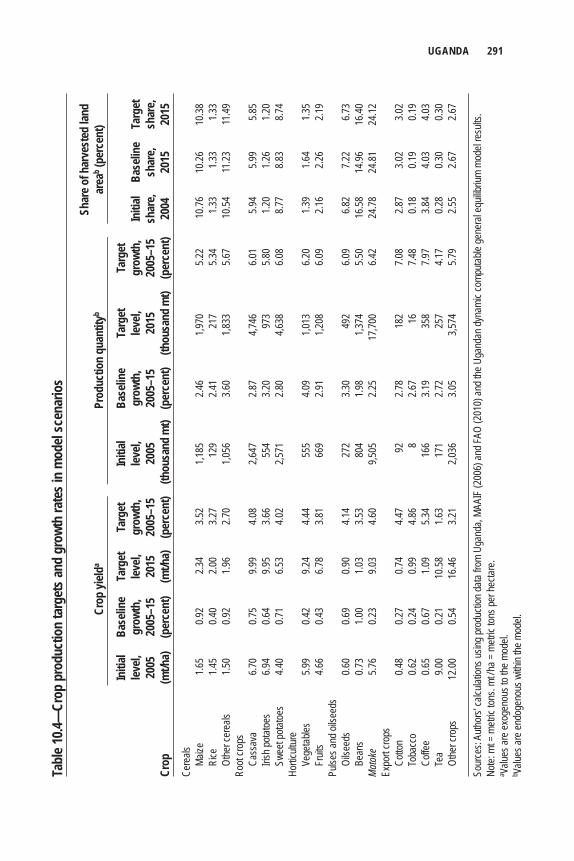
UGANDA 291Ta
ble 1
0.4—
Crop
pro
duct
ion
targ
ets a
nd g
rowt
h ra
tes i
n m
odel
scen
ario
s
Sh
are o
f har
vest
ed la
nd
Cr
op yi
elda
Prod
uctio
n qu
antit
yb ar
eab (p
erce
nt)
In
itial
Base
line
Targ
et
Targ
et
Initi
al Ba
selin
e Ta
rget
Ta
rget
level,
gr
owth
, lev
el,
grow
th,
level,
gr
owth
, lev
el,
grow
th,
Initi
al Ba
selin
e Ta
rget
20
05
2005
–15
2015
20
05–1
5 20
05
2005
–15
2015
20
05–1
5 sh
are,
shar
e, sh
are,
Crop
(m
t/ha)
(p
erce
nt)
(mt/h
a)
(per
cent
) (t
hous
and
mt)
(per
cent
) (th
ousa
nd m
t) (p
erce
nt)
2004
20
15
2015
Cere
als
Maize
1.6
5 0.9
2 2.3
4 3.5
2 1,1
85
2.46
1,970
5.2
2 10
.76
10.26
10
.38
Rice
1.4
5 0.4
0 2.0
0 3.2
7 12
9 2.4
1 21
7 5.3
4 1.3
3 1.3
3 1.3
3
Othe
r cer
eals
1.5
0 0.9
2 1.9
6 2.7
0 1,0
56
3.60
1,833
5.6
7 10
.54
11.23
11
.49Ro
ot cro
ps
Cass
ava
6.70
0.75
9.99
4.08
2,647
2.8
7 4,7
46
6.01
5.94
5.99
5.85
Iris
h pota
toes
6.94
0.64
9.95
3.66
554
3.20
973
5.80
1.20
1.26
1.20
Sw
eet p
otatoe
s 4.4
0 0.7
1 6.5
3 4.0
2 2,5
71
2.80
4,638
6.0
8 8.7
7 8.8
3 8.7
4Ho
rticult
ure
Ve
getab
les
5.99
0.42
9.24
4.44
555
4.09
1,013
6.2
0 1.3
9 1.6
4 1.3
5
Fruit
s 4.6
6 0.4
3 6.7
8 3.8
1 66
9 2.9
1 1,2
08
6.09
2.16
2.26
2.19
Pulse
s and
oilse
eds
Oi
lseed
s 0.6
0 0.6
9 0.9
0 4.1
4 27
2 3.3
0 49
2 6.0
9 6.8
2 7.2
2 6.7
3
Bean
s 0.7
3 1.0
0 1.0
3 3.5
3 80
4 1.9
8 1,3
74
5.50
16.58
14
.96
16.40
Mat
oke
5.76
0.23
9.03
4.60
9,505
2.2
5 17
,700
6.42
24.78
24
.81
24.12
Expo
rt cro
ps
Cotto
n 0.4
8 0.2
7 0.7
4 4.4
7 92
2.7
8 18
2 7.0
8 2.8
7 3.0
2 3.0
2
Toba
cco
0.62
0.24
0.99
4.86
8 2.6
7 16
7.4
8 0.1
8 0.1
9 0.1
9
Coffe
e 0.6
5 0.6
7 1.0
9 5.3
4 16
6 3.1
9 35
8 7.9
7 3.8
4 4.0
3 4.0
3
Tea
9.00
0.21
10.58
1.6
3 17
1 2.7
2 25
7 4.1
7 0.2
8 0.3
0 0.3
0
Othe
r cro
ps
12.00
0.5
4 16
.46
3.21
2,036
3.0
5 3,5
74
5.79
2.55
2.67
2.67
Sour
ces:
Autho
rs’ ca
lculat
ions u
sing p
rodu
ction
data
from
Ugan
da, M
AAIF
(200
6) an
d FAO
(201
0) an
d the
Uga
ndan
dyna
mic c
ompu
table
gene
ral e
quilib
rium
mode
l resu
lts.
Note:
mt =
metr
ic ton
s. mt
/ ha =
metr
ic ton
s per
hecta
re.
a Value
s are
exog
enou
s to t
he m
odel.
b Value
s are
endo
geno
us w
ithin
the m
odel.
292 SAMUEL BENIN ET AL.
the physical amount of land allocated to cereal crops rises by 2015. Rising yields and expanding land areas cause maize production to grow at about 2.5 percent per year during 2005–15. Thus, in the baseline, we see small but stable improvements in cereal yields over the simulation periods, with modest production growth driven by population-driven land expansion. Because cereal production growth is less than population growth, annual average per capita cereal consumption falls from 29.0 to 26.3 kilograms by 2015.
Based on observed root-crop production trends, we assume that these crops’ yields will grow at rates similar to those of cereal yields over the coming decade. Cassava yields in the baseline grow at 0.75 percent per year. Cassava dryweight yields gradually rise from 6.7 mt/ha to 7.2 mt/ha by 2015, which is equivalent to the his-torical peak yield achieved in 2005. The slow pace of cassava yield growth in the baseline is consistent with the relatively constant yields achieved since 1999. Similarly, Irish potato yields rise to 7.4 mt/ha, which is well below the 8.4 metric tons achieved during the mid-1990s but is consistent with recent trends. Land allocations to root crops are expected to remain relatively constant despite the overall land expansion of 2 percent per year. Thus, production grows at about 3 percent per year for root crops as a whole, which is only slightly faster than cereal production growth.
Observed trends indicate that the performance of other foodcrops has been mixed. Fruits have not performed well, with production growing at only 0.7 percent per year during 1990–2006. Vegetables have performed better, with production growing at about 3 percent per year. Thus, the baseline scenario assumes faster growth in vegetables compared with fruits and cereals. Groundnut production has also risen since 2000, and this trend is assumed to continue and be supported by increased land allocations. Accordingly, the production of oilseed crops grows at 3.3 percent per year, which is faster than the average growth rate of the overall agricul-tural sector.
Export crops play a key role in the agricultural sector, generating 9.5 percent of the sector’s GDP and a far larger share of the country’s export earnings (see Table 10.3). These export crops are also likely to have greater growth potential than many staple food crops, as observed during 2006–09 (Uganda, BOS 2010). Despite this potential, agricultural exports have performed poorly over the whole of the past decade, with crop yields falling for tea and tobacco. The baseline scenario assumes that the performance of these crops improves slightly during 2005–15. Annual yield growth ranges from 0.21 percent for tea to 0.67 percent for coffee (see Table 10.4). Coffee is especially important for Uganda, as more than 1 million farm households are engaged in coffee production (see Table 10.1). Since 2002, there has been a sharp drop in coffee production by about 25 percent. The baseline scenario assumes that this downward trend is halted and that production rises to 227,000 metric tons by
UGANDA 293
2015, which is still below the production levels achieved in the late 1990s. The baseline scenario, therefore, assumes a modest recovery of the coffee sector.
Livestock is an important agricultural subsector, generating 14 percent of agri-cultural GDP in 2005. Recent evidence suggests that Uganda’s livestock population has been growing steadily (FAO 2010). We assume that these stock trends are indicative of changes in livestock value-added. Cattle GDP in the baseline grows at 2.8 percent per year during 2005–15, which is slightly lower than the cattle popula-tion’s annual growth rate of 3.6 percent during 1998–2006. The poultry population has also grown rapidly since 1998, although there was a sharp decline in 2006. The baseline scenario assumes that the poultry population will return to longer-term trends and that the poultry GDP will grow at 2.6 percent per year during 2005–15. Finally, the populations of other livestock types have not grown as fast as those of either cattle or poultry over the past decade (for example, the pig population grew at only 1.8 percent per year during 1998–2006). The baseline scenario therefore assumes that other livestock GDP grows at about 2 percent per year.
Fisheries and forestry together generate about 13.5 percent of total agricultural GDP. The baseline assumes that fi sheries GDP will grow at 2.7 percent per year during 2005–15. This value captures reasonable expectations about Uganda’s natu-ral potential for expanding this sector, but it also refl ects the typical challenges associated with capture fi sheries. More specifi cally, we assume that fi sh production grows from 416,000 metric tons in 2005 to 541,000 metric tons in 2015, which is equivalent to achieving the production targets identifi ed in the government’s stra-tegic export plan, but by 2015 as opposed to the 2007 goal stated in the plan. Recent evidence for the forestry subsector suggests that growth has been driven by charcoal and fuel wood production for household use (Kebba and Ofwono 2007). The baseline scenario therefore assumes that forestry GDP will grow roughly in propor-tion to the population at around 3.1 percent per year during 2005–15.
Drawing on these detailed trends, the DCGE model indicates that, with mod-est growth in the agricultural sector and more rapid growth in nonagricultural sectors, overall national GDP will grow at an average rate of 5.1 percent during 2005–15 (see Table 10.3). This rate is close to the average GDP growth rate of about 5.5 percent since 2000. The population grows at 3.2 percent per year, so per capita GDP growth is 1.9 percent. With rising per capita incomes, the model indicates that poverty will decline modestly: national poverty will fall from 31.1 percent in 2004 to 26.5 percent in 2015. This is enough for Uganda to reach the fi rst Millennium Development Goal (MDG1) of halving the 1990 poverty rate by 2015 (Figure 10.2). However, with such modest poverty reduction and an expanding population, the absolute number of poor people in Uganda will increase from about 8.4 million in 2005 to 10.2 million by 2015. The model results indicate that urban
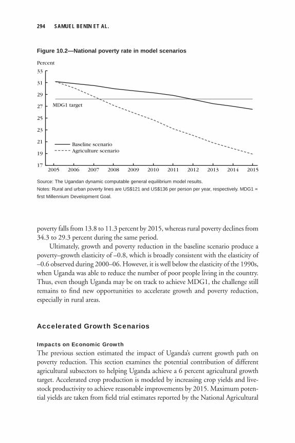
294 SAMUEL BENIN ET AL.
poverty falls from 13.8 to 11.3 percent by 2015, whereas rural poverty declines from 34.3 to 29.3 percent during the same period.
Ultimately, growth and poverty reduction in the baseline scenario produce a poverty–growth elasticity of –0.8, which is broadly consistent with the elasticity of –0.6 observed during 2000–06. However, it is well below the elasticity of the 1990s, when Uganda was able to reduce the number of poor people living in the country. Thus, even though Uganda may be on track to achieve MDG1, the challenge still remains to fi nd new opportunities to accelerate growth and poverty reduction, especially in rural areas.
Accelerated Growth Scenarios
Impacts on Economic GrowthThe previous section estimated the impact of Uganda’s current growth path on poverty reduction. This section examines the potential contribution of different agricultural subsectors to helping Uganda achieve a 6 percent agricultural growth target. Accelerated crop production is modeled by increasing crop yields and live-stock productivity to achieve reasonable improvements by 2015. Maximum poten-tial yields are taken from fi eld trial estimates reported by the National Agricultural
Percent
33
Baseline scenario
MDG1 target
17
31
29
27
25
23
21
19
20152014201320122011201020092008200720062005
Agriculture scenario
Figure 10.2—National poverty rate in model scenarios
Source: The Ugandan dynamic computable general equilibrium model results.Notes: Rural and urban poverty lines are US$121 and US$136 per person per year, respectively. MDG1 = first Millennium Development Goal.
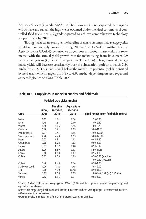
UGANDA 295
Advisory Services (Uganda, MAAIF 2006). However, it is not expected that Uganda will achieve and sustain the high yields obtained under the ideal conditions of con-trolled fi eld trials, nor is Uganda expected to achieve comprehensive technology adoption rates by 2015.
Taking maize as an example, the baseline scenario assumes that average yields would remain roughly constant during 2005–15 at 1.65–1.81 mt/ha. For the Agriculture, or CAADP, scenario, we target more ambitious maize yield improve-ments, with the annual yield growth rate for maize rising from its current 0.9 percent per year to 3.5 percent per year (see Table 10.4). Thus, national average maize yields will increase consistently over the simulation periods to reach 2.34 mt/ha by 2015. This level is well below the maximum potential yields identifi ed by fi eld trials, which range from 1.25 to 4.90 mt/ha, depending on seed types and agroecological conditions (Table 10.5).
Table 10.5—Crop yields in model scenarios and field trials
Modeled crop yields (mt/ha)
Baseline Agriculture Initial, scenario, scenario,Crop 2005 2015 2015 Yield ranges from field trials (mt/ha)Maize 1.65 1.81 2.34 1.25–4.90Rice 1.45 1.51 2.00 1.40–2.60Wheat 1.50 1.65 1.96 1.80–3.75Cassava 6.70 7.21 9.99 5.00–11.50Irish potatoes 6.94 7.41 9.95 4.50–12.50Sweet potatoes 4.40 4.73 6.53 5.00–12.00Beans 0.73 0.81 1.03 0.45–1.20Groundnuts 0.68 0.73 1.02 0.50–1.00Simsim 0.53 0.57 0.80 0.53–0.98Matoke 5.76 5.89 9.03 5.50–11.88Cocoa 0.60 0.63 0.82 0.55–1.00Coffee 0.65 0.69 1.09 0.50–0.95 (arabica) 1.00–2.50 (robusta)Cotton 0.48 0.49 0.74 0.28–1.00Sunflower seeds 1.06 1.12 1.45 1.05–2.00Tea 9.00 9.20 10.58 8.50–11.50Tobaccoa 0.62 0.63 0.99 1.00 (fire), 1.20 (air), 1.45 (flue)Vanilla 0.52 0.55 0.71 0.68–1.50
Sources: Authors’ calculations using Uganda, MAAIF (2006) and the Ugandan dynamic computable general equilibrium model results.Notes: Yield ranges begin with traditional, low-input practices and end with high-input, recommended practices. mt/ha = metric tons per hectare.aMaximum yields are shown for different curing processes: fire, air, and flue.
296 SAMUEL BENIN ET AL.
Although the Agriculture scenario targets yields below those obtained in fi eld trials, recent trends in maize yields indicate that reaching and sustaining 2.34 mt/ha by 2015 will pose considerable challenges. Historical production data indicate that national average maize yields did not exceed 1.8 mt/ha during 1990–2005 (FAO 2010). Thus, the government would not only have to improve the distribu-tion of higher yielding seed technology but also improve current farming practices and the distribution of other inputs if it is to help farmers signifi cantly increase maize yields by 2015. For these reasons, 2.34 mt/ha is considered an ambitious maize yield target. Table 10.5 provides similar comparisons between modeled and fi eld trial yields for other selected crops.
Agriculture’s current poor performance means that achieving the 6 percent agricultural growth target will be challenging, as Uganda will have to more than double its baseline agricultural growth rate. However, the DCGE model indicates that 6 percent agricultural growth is possible if the sector-level targets for crop yields and productivity are achieved. Because agriculture accounts for one-third of the economy, this acceleration of agricultural growth would raise the national GDP growth rate from its current 5.1 percent to 6.1 percent per year during 2005–15 (see Table 10.3). Faster agricultural growth would stimulate additional growth in the nonagricultural sectors by raising fi nal demand for nonagricultural goods, lower-ing input prices, and fostering upstream processing. In the Agriculture growth scenario, the GDP growth rate of the processing sectors would increase from 4.4 percent in the baseline scenario to 5.8 percent per year. Therefore, accelerating agricultural growth has economywide growth-linkage effects for nonagriculture.
Faster agricultural growth and its spillover effects cause poverty to decline by a further 7.6 percentage points, from the baseline rate of 26.5 percent in 2015 to 18.9 percent under the Agriculture scenario. Higher agricultural growth means that overall economic growth in Uganda becomes more broadly based. The poverty–growth elasticity rises from 0.8 to 1.7 (in terms of absolute value), which is now similar to the elasticity achieved during the 1990s. Moreover, taking population growth into account, achieving the 6 percent agricultural growth target lifts an additional 2.9 million people above the poverty line by 2015 and is suffi cient to reverse current trends by reducing the absolute number of poor people in Uganda by 2015.
Impacts on Household Incomes and PovertyFaster agricultural growth would benefi t most households. However, not all house-holds benefi t equally from achieving the yield targets. Table 10.6 shows changes in poverty rates for the different farm types and household groups in the model. Additional growth in the Agriculture scenario is partly driven by expanding export crops, whose GDP growth rises from 2.9 to 7.1 percent per year (see Table 10.3).
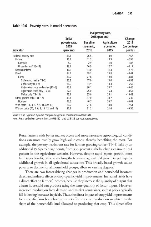
UGANDA 297
Rural farmers with better market access and more favorable agroecological condi-tions can more readily grow high-value crops, thereby benefi ting the most. For example, the poverty headcount rate for farmers growing coffee (T3–4) falls by an additional 15.6 percentage points, from 33.9 percent in the baseline scenario to 18.4 percent in the Agriculture scenario. However, despite rapid export growth, most farm types benefi t, because reaching the 6 percent agricultural growth target requires additional growth in all agricultural subsectors. This broadly based growth causes poverty to decline for all household groups, albeit to varying degrees.
There are two forces driving changes in production and household incomes: direct and indirect effects of crop-specifi c yield improvements. Increased yields have a direct effect on farmers’ incomes, because they increase the quantity of output that a farm household can produce using the same quantity of factor inputs. However, increased production faces demand and market constraints, so that prices typically fall following increases in yields. Thus, the direct impact of crop yield improvements for a specifi c farm household is its net effect on crop production weighted by the share of the household’s land allocated to producing that crop. This direct effect
Table 10.6—Poverty rates in model scenarios
Initial Change, poverty rate, Baseline Agriculture 2015 2005 scenario, scenario, (percentage Indicator (percent) 2015 2015 points)National poverty rate 31.1 26.5 18.9 –7.57 Urban 13.8 11.3 8.3 –2.95 Kampala 4.9 2.9 1.0 –1.87 Urban farms (T13–14) 19.7 16.9 12.7 –4.17 Urban nonfarm 16.5 14.0 11.3 –2.72 Rural 34.3 29.3 20.8 –8.41 Farm 33.2 27.8 19.0 –8.84 Coffee and maize (T1–2) 23.2 17.0 10.0 –6.93 Coffee only (T3–4) 36.9 33.9 18.4 –15.55 High-value crops and maize (T5–6) 35.9 30.1 20.7 –9.40 High-value crops only (T7–8) 27.5 25.0 16.4 –8.53 Maize only (T9–10) 42.1 35.6 25.1 –10.42 Other staples only (T11–12) 43.1 37.0 30.7 –6.30 Nonfarm 42.6 40.7 35.7 –5.01 With cattle (T1, 3, 5, 7, 9, 11, and 13) 26.2 21.6 14.0 –7.51 Without cattle (T2, 4, 6, 8, 10, 12, and 14) 37.1 31.2 21.6 –9.56
Source: The Ugandan dynamic computable general equilibrium model results.Note: Rural and urban poverty lines are US$121 and US$136 per year, respectively.
Final poverty rate, 2015 (percent)
298 SAMUEL BENIN ET AL.
assumes that land allocations remain fi xed. However, farmers may reallocate land in response to changes in relative prices. Thus, the indirect impact of crop yield improvements is the potentially positive impact of reallocating land to other crops. The DCGE model captures both the direct and indirect effects of crop yield improvements.
The model results indicate that urban agriculturalists also benefi t in the Agriculture scenario. This result can be seen in Table 10.6, which shows that urban farm households’ poverty rates decline by an additional 4.2 percentage points per year in the Agriculture scenario. Nonfarm households also benefi t from lower food prices (see below). However, because rural poverty is initially much higher than urban poverty and agriculture is especially important for poorer rural households, the poverty rate for rural farm households declines by an additional 8.4 percentage points.
Price Effects and Marketing ConstraintsFigure 10.3 shows the importance of taking demand constraints and relative price changes into account. Matoke has relatively weak linkages to upstream food process-ing, and therefore faces more stringent demand constraints to increasing produc-tion. These constraints cause matoke prices to decline signifi cantly in the Agriculture scenario. Maize has slightly stronger linkages to the animal-feed and food-processing sectors, which means that although maize prices decline under faster growth, they fall by less than matoke prices. Finally, the farmgate coffee price is infl uenced by Uganda’s real exchange rate, which depreciates in the Agriculture scenario. Thus, the price received by coffee farmers rises slightly despite higher coffee production. These price changes cause farmers to reallocate land away from crops that become less profi table, so the share of land planted in maize and matoke declines, while that allocated to export crops increases (see the last three columns of Table 10.4).
Prioritizing Agricultural Subsectors for InvestmentSo far we have examined the poverty impact of accelerating agricultural growth to 6 percent per year. However, understanding how poverty–growth linkages vary at the subsector and household levels is important for designing pro-poor growth strategies. Therefore, we now prioritize specifi c crops and subsectors for investment.
We fi rst calculate poverty–growth elasticities that allow us to compare the pro-poorness of growth in alternative subsectors. These elasticities are endogenous outcomes from the model results. Growth affects individual households differently because of heterogeneity across household groups. The above analysis has shown how, given differences in household and farm characteristics, changes in income across households can differ considerably from average changes at the national level. Thus, to capture growth–poverty linkages, we must understand the changes in
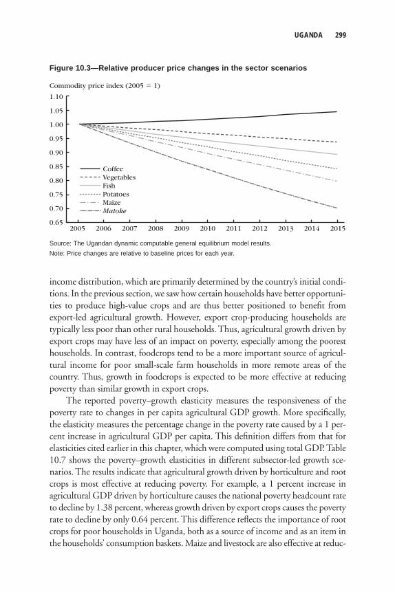
UGANDA 299
income distribution, which are primarily determined by the country’s initial condi-tions. In the previous section, we saw how certain households have better opportuni-ties to produce high-value crops and are thus better positioned to benefi t from export-led agricultural growth. However, export crop-producing households are typically less poor than other rural households. Thus, agricultural growth driven by export crops may have less of an impact on poverty, especially among the poorest households. In contrast, foodcrops tend to be a more important source of agricul-tural income for poor small-scale farm households in more remote areas of the country. Thus, growth in foodcrops is expected to be more effective at reducing poverty than similar growth in export crops.
The reported poverty–growth elasticity measures the responsiveness of the poverty rate to changes in per capita agricultural GDP growth. More specifi cally, the elasticity measures the percentage change in the poverty rate caused by a 1 per-cent increase in agricultural GDP per capita. This defi nition differs from that for elasticities cited earlier in this chapter, which were computed using total GDP. Table 10.7 shows the poverty–growth elasticities in different subsector-led growth sce-narios. The results indicate that agricultural growth driven by horticulture and root crops is most effective at reducing poverty. For example, a 1 percent increase in agricultural GDP driven by horticulture causes the national poverty headcount rate to decline by 1.38 percent, whereas growth driven by export crops causes the poverty rate to decline by only 0.64 percent. This difference refl ects the importance of root crops for poor households in Uganda, both as a source of income and as an item in the households’ consumption baskets. Maize and livestock are also effective at reduc-
CoffeeVegetables
Maize
FishPotatoes
Matoke
Commodity price index (2005 � 1)
1.10
0.65
1.05
1.00
0.95
0.90
0.85
0.80
0.75
0.70
20152014201320122011201020092008200720062005
Figure 10.3—Relative producer price changes in the sector scenarios
Source: The Ugandan dynamic computable general equilibrium model results.Note: Price changes are relative to baseline prices for each year.
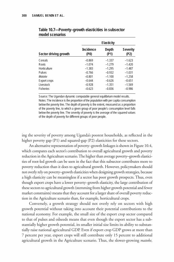
300 SAMUEL BENIN ET AL.
ing the severity of poverty among Uganda’s poorest households, as refl ected in the higher poverty gap (P1) and squared-gap (P2) elasticities for these sectors.
An alternative representation of poverty–growth linkages is shown in Figure 10.4, which compares each sector’s contribution to overall agricultural growth and poverty reduction in the Agriculture scenario. The higher than average poverty–growth elastici-ties of root-led growth can be seen in the fact that this subsector contributes more to poverty reduction than it does to agricultural growth. However, policymakers should not overly rely on poverty–growth elasticities when designing growth strategies, because a high elasticity can be meaningless if a sector has poor growth prospects. Thus, even though export crops have a lower poverty–growth elasticity, the large contribution of these sectors to agricultural growth (stemming from higher growth potential and fewer market constraints) means that they account for a larger share of overall poverty reduc-tion in the Agriculture scenario than, for example, horticultural crops.
Conversely, a growth strategy should not overly rely on sectors with high growth potential without taking into account their potential contributions to the national economy. For example, the small size of the export crop sector compared to that of pulses and oilseeds means that even though the export sector has a sub-stantially higher growth potential, its smaller initial size limits its ability to substan-tially raise national agricultural GDP. Even if export crop GDP grows at more than 7 percent per year, export crops will still contribute only 15 percent to additional agricultural growth in the Agriculture scenario. Thus, the slower-growing matoke,
Table 10.7—Poverty–growth elasticities in subsector model scenarios
Elasticity
Incidence Depth SeveritySector driving growth (P0) (P1) (P2)Cereals –0.869 –1.337 –1.623Roots –1.074 –1.279 –1.420Horticulture –1.383 –1.295 –1.487Pulses –0.766 –0.932 –1.031Matoke –0.801 –1.100 –1.258Export crops –0.644 –0.626 –0.651Livestock –0.928 –1.351 –1.569Fisheries –0.623 –0.836 –0.986
Source: The Ugandan dynamic computable general equilibrium model results.Notes: The incidence is the proportion of the population with per capita consumption below the poverty line. The depth of poverty is the extent, measured as a proportion of the poverty line, to which a given group of poor people’s consumption level falls below the poverty line. The severity of poverty is the average of the squared values of the depth of poverty for different groups of poor people.
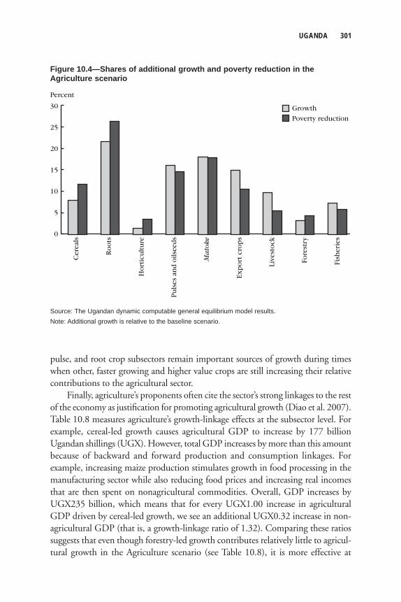
UGANDA 301
pulse, and root crop subsectors remain important sources of growth during times when other, faster growing and higher value crops are still increasing their relative contributions to the agricultural sector.
Finally, agriculture’s proponents often cite the sector’s strong linkages to the rest of the economy as justifi cation for promoting agricultural growth (Diao et al. 2007). Table 10.8 measures agriculture’s growth-linkage effects at the subsector level. For example, cereal-led growth causes agricultural GDP to increase by 177 billion Ugandan shillings (UGX). However, total GDP increases by more than this amount because of backward and forward production and consumption linkages. For example, increasing maize production stimulates growth in food processing in the manufacturing sector while also reducing food prices and increasing real incomes that are then spent on nonagricultural commodities. Overall, GDP increases by UGX235 billion, which means that for every UGX1.00 increase in agricultural GDP driven by cereal-led growth, we see an additional UGX0.32 increase in non-agricultural GDP (that is, a growth-linkage ratio of 1.32). Comparing these ratios suggests that even though forestry-led growth contributes relatively little to agricul-tural growth in the Agriculture scenario (see Table 10.8), it is more effective at
Cer
eals
Ro
ots
Ma
toke
Exp
ort
cro
ps
Live
sto
ck
Ho
rtic
ult
ure
Pu
lses
an
d o
ilsee
ds
Fore
stry
Fish
erie
s
Poverty reduction
Growth
Percent
30
0
25
20
15
10
5
Figure 10.4—Shares of additional growth and poverty reduction in the Agriculture scenario
Source: The Ugandan dynamic computable general equilibrium model results.Note: Additional growth is relative to the baseline scenario.
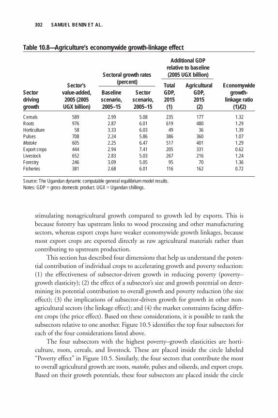
302 SAMUEL BENIN ET AL.
stimulating nonagricultural growth compared to growth led by exports. This is because forestry has upstream links to wood processing and other manufacturing sectors, whereas export crops have weaker economywide growth linkages, because most export crops are exported directly as raw agricultural materials rather than contributing to upstream production.
This section has described four dimensions that help us understand the poten-tial contribution of individual crops to accelerating growth and poverty reduction: (1) the effectiveness of subsector-driven growth in reducing poverty (poverty–growth elasticity); (2) the effect of a subsector’s size and growth potential on deter-mining its potential contribution to overall growth and poverty reduction (the size effect); (3) the implications of subsector-driven growth for growth in other non-agricultural sectors (the linkage effect); and (4) the market constraints facing differ-ent crops (the price effect). Based on these considerations, it is possible to rank the subsectors relative to one another. Figure 10.5 identifi es the top four subsectors for each of the four considerations listed above.
The four subsectors with the highest poverty–growth elasticities are horti-culture, roots, cereals, and livestock. These are placed inside the circle labeled “Poverty effect” in Figure 10.5. Similarly, the four sectors that contribute the most to overall agricultural growth are roots, matoke, pulses and oilseeds, and export crops. Based on their growth potentials, these four subsectors are placed inside the circle
Table 10.8—Agriculture’s economywide growth-linkage effect
Additional GDP relative to baseline (2005 UGX billion)
Sector’s Total Agricultural EconomywideSector value-added, Baseline Sector GDP, GDP, growth-driving 2005 (2005 scenario, scenario, 2015 2015 linkage ratiogrowth UGX billion) 2005–15 2005–15 (1) (2) (1)/(2)Cereals 589 2.99 5.08 235 177 1.32Roots 976 2.87 6.01 619 480 1.29Horticulture 58 3.33 6.03 49 36 1.39Pulses 708 2.24 5.86 386 360 1.07Matoke 605 2.25 6.47 517 401 1.29Export crops 444 2.94 7.41 205 331 0.62Livestock 652 2.83 5.03 267 216 1.24Forestry 246 3.09 5.05 95 70 1.36Fisheries 381 2.68 6.01 116 162 0.72
Source: The Ugandan dynamic computable general equilibrium model results.Notes: GDP = gross domestic product. UGX = Ugandan shillings.
Sectoral growth rates(percent)
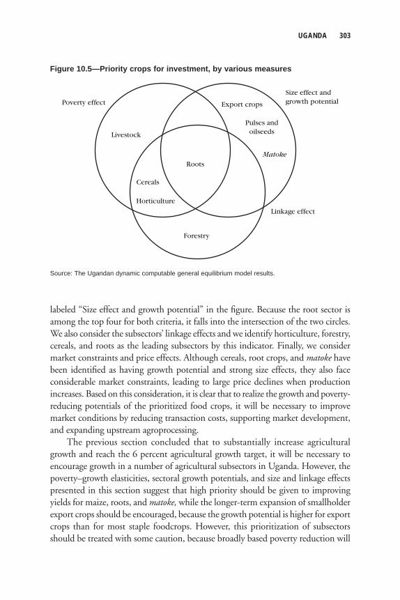
UGANDA 303
labeled “Size effect and growth potential” in the fi gure. Because the root sector is among the top four for both criteria, it falls into the intersection of the two circles. We also consider the subsectors’ linkage effects and we identify horticulture, forestry, cereals, and roots as the leading subsectors by this indicator. Finally, we consider market constraints and price effects. Although cereals, root crops, and matoke have been identifi ed as having growth potential and strong size effects, they also face considerable market constraints, leading to large price declines when production increases. Based on this consideration, it is clear that to realize the growth and poverty-reducing potentials of the prioritized food crops, it will be necessary to improve market conditions by reducing transaction costs, supporting market development, and expanding upstream agroprocessing.
The previous section concluded that to substantially increase agricultural growth and reach the 6 percent agricultural growth target, it will be necessary to encourage growth in a number of agricultural subsectors in Uganda. However, the poverty–growth elasticities, sectoral growth potentials, and size and linkage effects presented in this section suggest that high priority should be given to improving yields for maize, roots, and matoke, while the longer-term expansion of smallholder export crops should be encouraged, because the growth potential is higher for export crops than for most staple foodcrops. However, this prioritization of subsectors should be treated with some caution, because broadly based poverty reduction will
Poverty effect
Size effect andgrowth potentialExport crops
Pulses andoilseedsLivestock
MatokeRoots
Cereals
Horticulture
Linkage effect
Forestry
Figure 10.5—Priority crops for investment, by various measures
Source: The Ugandan dynamic computable general equilibrium model results.
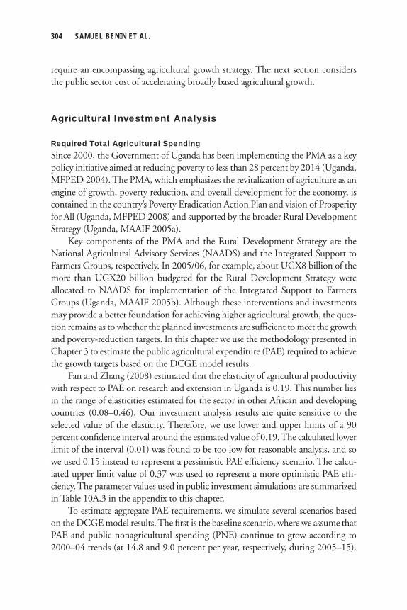
304 SAMUEL BENIN ET AL.
require an encompassing agricultural growth strategy. The next section considers the public sector cost of accelerating broadly based agricultural growth.
Agricultural Investment Analysis
Required Total Agricultural Spending Since 2000, the Government of Uganda has been implementing the PMA as a key policy initiative aimed at reducing poverty to less than 28 percent by 2014 (Uganda, MFPED 2004). The PMA, which emphasizes the revitalization of agriculture as an engine of growth, poverty reduction, and overall development for the economy, is contained in the country’s Poverty Eradication Action Plan and vision of Prosperity for All (Uganda, MFPED 2008) and supported by the broader Rural Development Strategy (Uganda, MAAIF 2005a).
Key components of the PMA and the Rural Development Strategy are the National Agricultural Advisory Services (NAADS) and the Integrated Support to Farmers Groups, respectively. In 2005/06, for example, about UGX8 billion of the more than UGX20 billion budgeted for the Rural Development Strategy were allocated to NAADS for implementation of the Integrated Support to Farmers Groups (Uganda, MAAIF 2005b). Although these interventions and investments may provide a better foundation for achieving higher agricultural growth, the ques-tion remains as to whether the planned investments are suffi cient to meet the growth and poverty-reduction targets. In this chapter we use the methodology presented in Chapter 3 to estimate the public agricultural expenditure (PAE) required to achieve the growth targets based on the DCGE model results.
Fan and Zhang (2008) estimated that the elasticity of agricultural productivity with respect to PAE on research and extension in Uganda is 0.19. This number lies in the range of elasticities estimated for the sector in other African and developing countries (0.08–0.46). Our investment analysis results are quite sensitive to the selected value of the elasticity. Therefore, we use lower and upper limits of a 90 percent confi dence interval around the estimated value of 0.19. The calculated lower limit of the interval (0.01) was found to be too low for reasonable analysis, and so we used 0.15 instead to represent a pessimistic PAE effi ciency scenario. The calcu-lated upper limit value of 0.37 was used to represent a more optimistic PAE effi -ciency. The parameter values used in public investment simulations are summarized in Table 10A.3 in the appendix to this chapter.
To estimate aggregate PAE requirements, we simulate several scenarios based on the DCGE model results. The fi rst is the baseline scenario, where we assume that PAE and public nonagricultural spending (PNE) continue to grow according to 2000–04 trends (at 14.8 and 9.0 percent per year, respectively, during 2005–15).
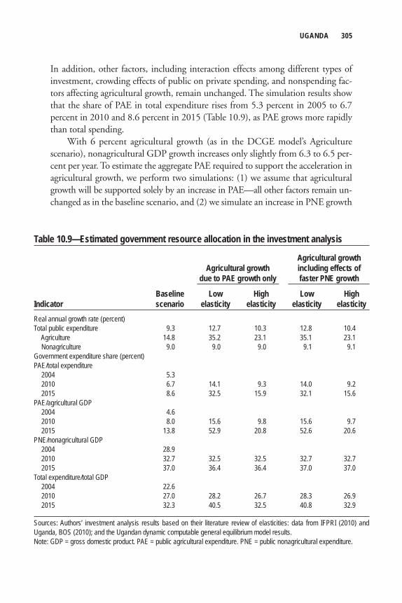
UGANDA 305
In addition, other factors, including interaction effects among different types of investment, crowding effects of public on private spending, and nonspending fac-tors affecting agricultural growth, remain unchanged. The simulation results show that the share of PAE in total expenditure rises from 5.3 percent in 2005 to 6.7 percent in 2010 and 8.6 percent in 2015 (Table 10.9), as PAE grows more rapidly than total spending.
With 6 percent agricultural growth (as in the DCGE model’s Agriculture scenario), nonagricultural GDP growth increases only slightly from 6.3 to 6.5 per-cent per year. To estimate the aggregate PAE required to support the acceleration in agricultural growth, we perform two simulations: (1) we assume that agricultural growth will be supported solely by an increase in PAE—all other factors remain un-changed as in the baseline scenario, and (2) we simulate an increase in PNE growth
Table 10.9—Estimated government resource allocation in the investment analysis
Agricultural growth Agricultural growth including effects of due to PAE growth only faster PNE growth
Baseline Low High Low HighIndicator scenario elasticity elasticity elasticity elasticityReal annual growth rate (percent)Total public expenditure 9.3 12.7 10.3 12.8 10.4 Agriculture 14.8 35.2 23.1 35.1 23.1 Nonagriculture 9.0 9.0 9.0 9.1 9.1Government expenditure share (percent)PAE/total expenditure 2004 5.3 2010 6.7 14.1 9.3 14.0 9.2 2015 8.6 32.5 15.9 32.1 15.6PAE/agricultural GDP 2004 4.6 2010 8.0 15.6 9.8 15.6 9.7 2015 13.8 52.9 20.8 52.6 20.6PNE/nonagricultural GDP 2004 28.9 2010 32.7 32.5 32.5 32.7 32.7 2015 37.0 36.4 36.4 37.0 37.0Total expenditure/total GDP 2004 22.6 2010 27.0 28.2 26.7 28.3 26.9 2015 32.3 40.5 32.5 40.8 32.9
Sources: Authors’ investment analysis results based on their literature review of elasticities: data from IFPRI (2010) and Uganda, BOS (2010); and the Ugandan dynamic computable general equilibrium model results.Note: GDP = gross domestic product. PAE = public agricultural expenditure. PNE = public nonagricultural expenditure.
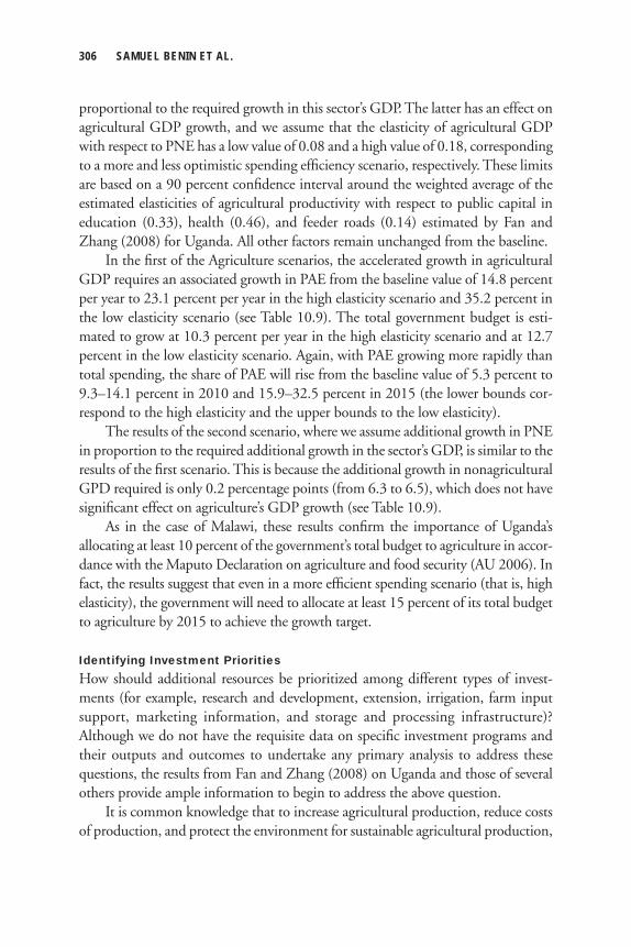
306 SAMUEL BENIN ET AL.
proportional to the required growth in this sector’s GDP. The latter has an effect on agricultural GDP growth, and we assume that the elasticity of agricultural GDP with respect to PNE has a low value of 0.08 and a high value of 0.18, corresponding to a more and less optimistic spending effi ciency scenario, respectively. These limits are based on a 90 percent confi dence interval around the weighted average of the estimated elasticities of agricultural productivity with respect to public capital in education (0.33), health (0.46), and feeder roads (0.14) estimated by Fan and Zhang (2008) for Uganda. All other factors remain unchanged from the baseline.
In the fi rst of the Agriculture scenarios, the accelerated growth in agricultural GDP requires an associated growth in PAE from the baseline value of 14.8 percent per year to 23.1 percent per year in the high elasticity scenario and 35.2 percent in the low elasticity scenario (see Table 10.9). The total government budget is esti-mated to grow at 10.3 percent per year in the high elasticity scenario and at 12.7 percent in the low elasticity scenario. Again, with PAE growing more rapidly than total spending, the share of PAE will rise from the baseline value of 5.3 percent to 9.3–14.1 percent in 2010 and 15.9–32.5 percent in 2015 (the lower bounds cor-respond to the high elasticity and the upper bounds to the low elasticity).
The results of the second scenario, where we assume additional growth in PNE in proportion to the required additional growth in the sector’s GDP, is similar to the results of the fi rst scenario. This is because the additional growth in nonagricultural GPD required is only 0.2 percentage points (from 6.3 to 6.5), which does not have signifi cant effect on agriculture’s GDP growth (see Table 10.9).
As in the case of Malawi, these results confi rm the importance of Uganda’s allocating at least 10 percent of the government’s total budget to agriculture in accor-dance with the Maputo Declaration on agriculture and food security (AU 2006). In fact, the results suggest that even in a more effi cient spending scenario (that is, high elasticity), the government will need to allocate at least 15 percent of its total budget to agriculture by 2015 to achieve the growth target.
Identifying Investment PrioritiesHow should additional resources be prioritized among different types of invest-ments (for example, research and development, extension, irrigation, farm input support, marketing information, and storage and processing infrastructure)? Although we do not have the requisite data on specifi c investment programs and their outputs and outcomes to undertake any primary analysis to address these questions, the results from Fan and Zhang (2008) on Uganda and those of several others provide ample information to begin to address the above question.
It is common knowledge that to increase agricultural production, reduce costs of production, and protect the environment for sustainable agricultural production,
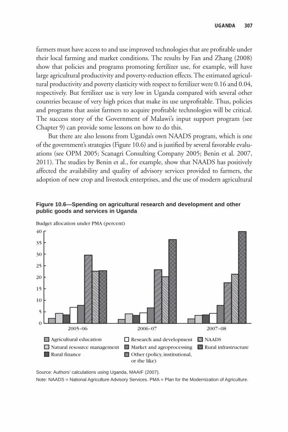
UGANDA 307
farmers must have access to and use improved technologies that are profi table under their local farming and market conditions. The results by Fan and Zhang (2008) show that policies and programs promoting fertilizer use, for example, will have large agricultural productivity and poverty-reduction effects. The estimated agricul-tural productivity and poverty elasticity with respect to fertilizer were 0.16 and 0.04, respectively. But fertilizer use is very low in Uganda compared with several other countries because of very high prices that make its use unprofi table. Thus, policies and programs that assist farmers to acquire profi table technologies will be critical. The success story of the Government of Malawi’s input support program (see Chapter 9) can provide some lessons on how to do this.
But there are also lessons from Uganda’s own NAADS program, which is one of the government’s strategies (Figure 10.6) and is justifi ed by several favorable evalu-ations (see OPM 2005; Scanagri Consulting Company 2005; Benin et al. 2007, 2011). The studies by Benin et al., for example, show that NAADS has positively affected the availability and quality of advisory services provided to farmers, the adoption of new crop and livestock enterprises, and the use of modern agricultural
2005–06
Budget allocation under PMA (percent)
40
0
25
20
35
30
15
10
5
2006–07 2007–08
Market and agroprocessingNatural resource management
Agricultural education Research and development
Rural finance
NAADS
Other (policy, institutional,or the like)
Rural infrastructure
Figure 10.6—Spending on agricultural research and development and other public goods and services in Uganda
Source: Authors’ calculations using Uganda, MAAIF (2007).Note: NAADS = National Agriculture Advisory Services. PMA = Plan for the Modernization of Agriculture.
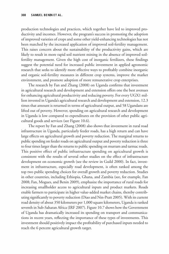
308 SAMUEL BENIN ET AL.
production technologies and practices, which together have led to improved pro-ductivity and incomes. However, the program’s success in promoting the adoption of improved varieties of crops and some other yield-enhancing technologies has not been matched by the increased application of improved soil-fertility management. This raises concern about the sustainability of the productivity gains, which are likely to result in more rapid soil nutrient mining in the absence of improved soil-fertility management. Given the high cost of inorganic fertilizers, these fi ndings suggest the potential need for increased public investment in applied agronomic research that seeks to identify more effective ways to profi tably combine inorganic and organic soil-fertility measures in different crop systems, improve the market environment, and promote adoption of more remunerative crop enterprises.
The research by Fan and Zhang (2008) on Uganda confi rms that investment in agricultural research and development and extension offers one the best avenues for enhancing agricultural productivity and reducing poverty. For every UGX1 mil-lion invested in Uganda’s agricultural research and development and extension, 12.3 times that amount is returned in terms of agricultural output, and 58 Ugandans are lifted out of poverty. However, spending on agricultural research and development in Uganda is low compared to expenditures on the provision of other public agri-cultural goods and services (see Figure 10.6).
The report by Fan and Zhang (2008) also shows that investment in rural road infrastructure in Uganda, particularly feeder roads, has a high return and can have large effects on agricultural growth and poverty reduction. The marginal returns to public spending on feeder roads on agricultural output and poverty reduction is three to four times larger than the returns to public spending on murram and tarmac roads. This positive effect of public infrastructure spending on agricultural growth is consistent with the results of several other studies on the effect of infrastructure development on economic growth (see the review in Guild 2000). In fact, invest-ment in infrastructure, especially road development, is often ranked among the top two public spending choices for overall growth and poverty reduction. Studies in other countries, including Ethiopia, Ghana, and Zambia (see, for example, Fan 2008; Fan, Mogues, and Benin 2009), emphasize the importance of rural roads for increasing smallholder access to agricultural inputs and product markets. Roads enable farmers to participate in higher value-added market chains, thereby contrib-uting signifi cantly to poverty reduction (Diao and Nin-Pratt 2005). With its current road density of about 350 kilometers per 1,000 square kilometers, Uganda is ranked seventh in Sub-Saharan Africa (IRF 2007). Figure 10.7 shows how the Government of Uganda has dramatically increased its spending on transport and communica-tions in recent years, refl ecting the importance of these types of investments. This investment should positively impact the profi tability of purchased inputs needed to reach the 6 percent agricultural growth target.
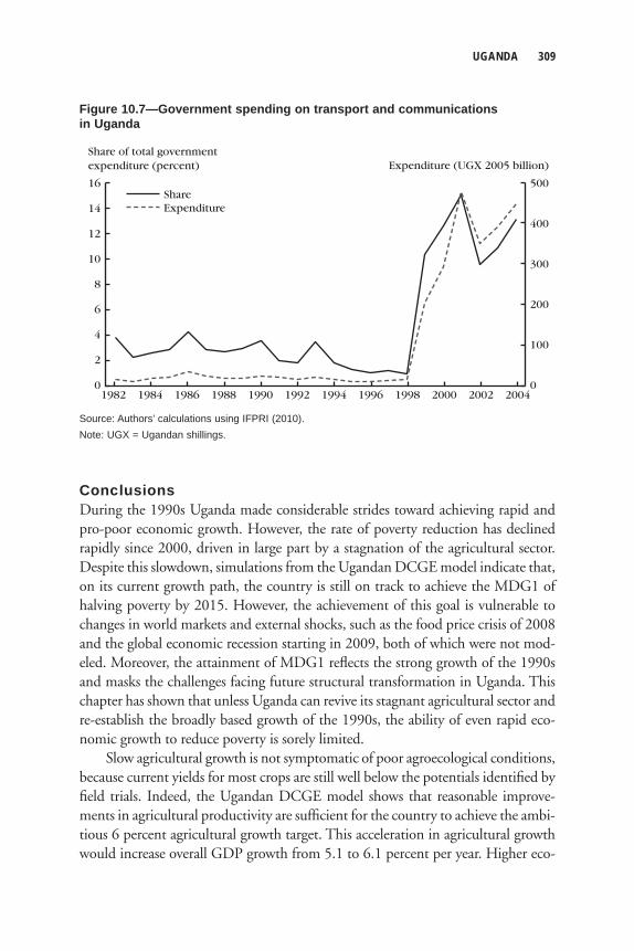
UGANDA 309
ConclusionsDuring the 1990s Uganda made considerable strides toward achieving rapid and pro-poor economic growth. However, the rate of poverty reduction has declined rapidly since 2000, driven in large part by a stagnation of the agricultural sector. Despite this slowdown, simulations from the Ugandan DCGE model indicate that, on its current growth path, the country is still on track to achieve the MDG1 of halving poverty by 2015. However, the achievement of this goal is vulnerable to changes in world markets and external shocks, such as the food price crisis of 2008 and the global economic recession starting in 2009, both of which were not mod-eled. Moreover, the attainment of MDG1 refl ects the strong growth of the 1990s and masks the challenges facing future structural transformation in Uganda. This chapter has shown that unless Uganda can revive its stagnant agricultural sector and re-establish the broadly based growth of the 1990s, the ability of even rapid eco-nomic growth to reduce poverty is sorely limited.
Slow agricultural growth is not symptomatic of poor agroecological conditions, because current yields for most crops are still well below the potentials identifi ed by fi eld trials. Indeed, the Ugandan DCGE model shows that reasonable improve-ments in agricultural productivity are suffi cient for the country to achieve the ambi-tious 6 percent agricultural growth target. This acceleration in agricultural growth would increase overall GDP growth from 5.1 to 6.1 percent per year. Higher eco-
Share of total governmentexpenditure (percent) Expenditure (UGX 2005 billion)
16
0
14
12
10
200419901988198619841982
8
6
4
2
500
0
400
300
200
100
1992 1994 1996 1998 2000 2002
ShareExpenditure
Figure 10.7—Government spending on transport and communications in Uganda
Source: Authors’ calculations using IFPRI (2010).Note: UGX = Ugandan shillings.
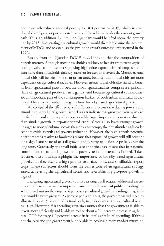
310 SAMUEL BENIN ET AL.
nomic growth reduces national poverty to 18.9 percent by 2015, which is lower than the 26.5 percent poverty rate that would be achieved under the current growth path. Thus, an additional 2.9 million Ugandans would be lifted above the poverty line by 2015. Accelerating agricultural growth would therefore ensure the achieve-ment of MDG1 and re-establish the pro-poor growth outcomes experienced in the 1990s.
Results from the Ugandan DCGE model indicate that the composition of growth matters. Although most households are likely to benefi t from faster agricul-tural growth, farm households growing high-value export-oriented crops stand to gain more than households that rely more on foodcrops or livestock. Moreover, rural households will benefi t more than urban ones, because rural households are more dependent on agricultural incomes. However, urban households also stand to bene-fi t from agricultural growth, because urban agriculturalists comprise a signifi cant share of agricultural producers in Uganda, and because agricultural commodities are an important part of the consumption baskets of both urban and rural house-holds. These results confi rm the gains from broadly based agricultural growth.
We compared the effectiveness of different subsectors on reducing poverty and stimulating agricultural growth. Model results indicate that growth driven by maize, horticulture, and root crops has considerably larger impacts on poverty reduction than similar growth in export-oriented crops. Cereals also have stronger growth linkages to nonagricultural sectors than do export crops, thereby stimulating broader economywide growth and poverty reduction. However, the high growth potential of export crops relative to foodcrops means that export-led growth will still account for a signifi cant share of overall growth and poverty reduction, especially over the long term. Conversely, the small initial size of horticulture means that its potential contribution to national growth and poverty reduction remains limited. Taken together, these fi ndings highlight the importance of broadly based agricultural growth, but they accord a high priority to maize, roots, and smallholder export crops. These subsectors should form the cornerstone of an agricultural strategy aimed at reviving the agricultural sector and re-establishing pro-poor growth in Uganda.
Increasing agricultural growth to meet its target will require additional invest-ment in the sector as well as improvements in the effi ciency of public spending. To achieve and sustain the targeted 6 percent agricultural growth, spending on agricul-ture would have to grow by 23 percent per year. Thus, the government will need to allocate at least 15 percent of its total budgetary resources to the agricultural sector by 2015. However, this spending scenario assumes that the government is able to invest more effi ciently and is able to realize about a 0.4 percent increase in agricul-tural GDP for every 1.0 percent increase in its total agricultural spending. If this is not the case and the government is only able to achieve a more modest return on
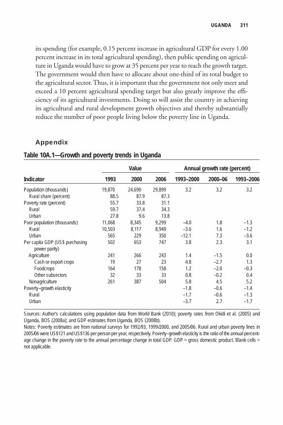
UGANDA 311
its spending (for example, 0.15 percent increase in agricultural GDP for every 1.00 percent increase in its total agricultural spending), then public spending on agricul-ture in Uganda would have to grow at 35 percent per year to reach the growth target. The government would then have to allocate about one-third of its total budget to the agricultural sector. Thus, it is important that the government not only meet and exceed a 10 percent agricultural spending target but also greatly improve the effi -ciency of its agricultural investments. Doing so will assist the country in achieving its agricultural and rural development growth objectives and thereby substantially reduce the number of poor people living below the poverty line in Uganda.
Appendix
Table 10A.1—Growth and poverty trends in Uganda
Value Annual growth rate (percent)
Indicator 1993 2000 2006 1993–2000 2000–06 1993–2006Population (thousands) 19,870 24,690 29,899 3.2 3.2 3.2 Rural share (percent) 88.5 87.9 87.3 Poverty rate (percent) 55.7 33.8 31.1 Rural 59.7 37.4 34.3 Urban 27.8 9.6 13.8 Poor population (thousands) 11,068 8,345 9,299 –4.0 1.8 –1.3 Rural 10,503 8,117 8,949 –3.6 1.6 –1.2 Urban 565 229 350 –12.1 7.3 –3.6Per capita GDP (US$ purchasing 502 653 747 3.8 2.3 3.1 power parity) Agriculture 241 266 243 1.4 –1.5 0.0 Cash or export crops 19 27 23 4.8 –2.7 1.3 Foodcrops 164 178 158 1.2 –2.0 –0.3 Other subsectors 32 33 33 0.8 –0.2 0.4 Nonagriculture 261 387 504 5.8 4.5 5.2Poverty–growth elasticity –1.8 –0.6 –1.4 Rural –1.7 –0.6 –1.3 Urban –3.7 2.7 –1.7
Sources: Author’s calculations using population data from World Bank (2010); poverty rates from Okidi et al. (2005) and Uganda, BOS (2008a); and GDP estimates from Uganda, BOS (2008b). Notes: Poverty estimates are from national surveys for 1992/93, 1999/2000, and 2005/06. Rural and urban poverty lines in 2005/06 were US$121 and US$136 per person per year, respectively. Poverty–growth elasticity is the ratio of the annual percent-age change in the poverty rate to the annual percentage change in total GDP. GDP = gross domestic product. Blank cells = not applicable.
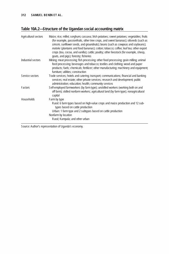
312 SAMUEL BENIN ET AL.
Table 10A.2—Structure of the Ugandan social accounting matrix
Agricultural sectors Maize; rice; millet; sorghum; cassava; Irish potatoes; sweet potatoes; vegetables; fruits (for example, passionfruits, other tree crops, and sweet bananas); oilseeds (such as
simsim, sunflower seeds, and groundnuts); beans (such as cowpeas and soybeans); matoke (plantains and food bananas); cotton; tobacco; coffee; leaf tea; other export crops (tea, cocoa, and vanilla); cattle; poultry; other livestock (for example, sheep, goats, and pigs); forestry; fisheries
Industrial sectors Mining; meat processing; fish processing; other food processing; grain milling; animal feed processing; beverages and tobacco; textiles and clothing; wood and paper
products; fuels; chemicals; fertilizer; other manufacturing; machinery and equipment; furniture; utilities; construction
Service sectors Trade services; hotels and catering; transport; communications; financial and banking services; real estate; other private services; research and development; public
administration; education; health; community servicesFactors Self-employed farmworkers (by farm type); unskilled workers (working both on and off farm); skilled nonfarm workers; agricultural land (by farm type); nonagricultural
capital Households Farm by type Rural: 6 farm types based on high-value crops and maize production and 12 sub- types based on cattle production Urban: 1 farm type and 2 subtypes based on cattle production Nonfarm by location Rural; Kampala; and other urban
Source: Author’s representation of Uganda’s economy.
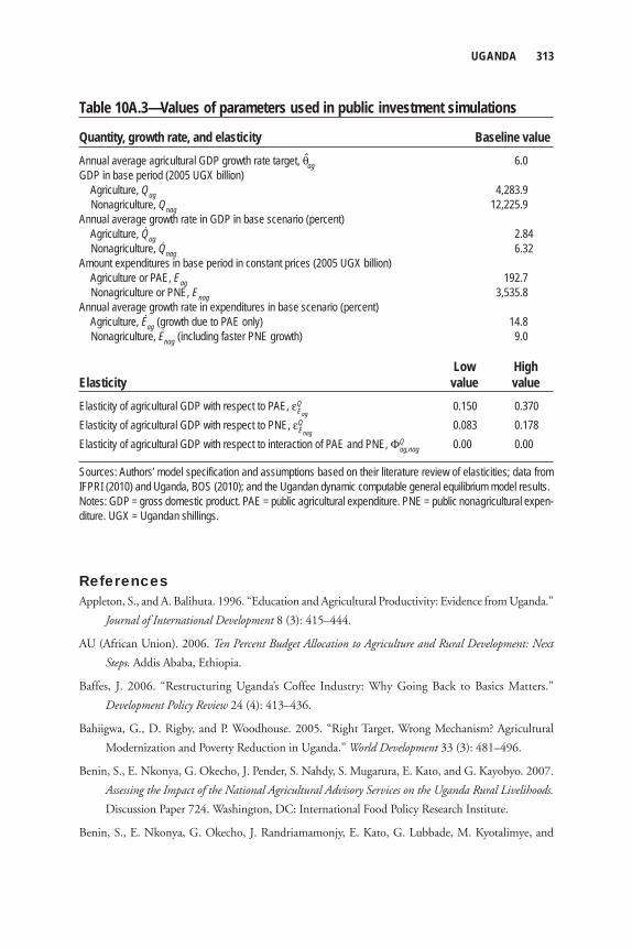
UGANDA 313
ReferencesAppleton, S., and A. Balihuta. 1996. “Education and Agricultural Productivity: Evidence from Uganda.”
Journal of International Development 8 (3): 415–444.
AU (African Union). 2006. Ten Percent Budget Allocation to Agriculture and Rural Development: Next
Steps. Addis Ababa, Ethiopia.
Baffes, J. 2006. “Restructuring Uganda’s Coffee Industry: Why Going Back to Basics Matters.”
Development Policy Review 24 (4): 413–436.
Bahiigwa, G., D. Rigby, and P. Woodhouse. 2005. “Right Target, Wrong Mechanism? Agricultural
Modernization and Poverty Reduction in Uganda.” World Development 33 (3): 481–496.
Benin, S., E. Nkonya, G. Okecho, J. Pender, S. Nahdy, S. Mugarura, E. Kato, and G. Kayobyo. 2007.
Assessing the Impact of the National Agricultural Advisory Services on the Uganda Rural Livelihoods.
Discussion Paper 724. Washington, DC: International Food Policy Research Institute.
Benin, S., E. Nkonya, G. Okecho, J. Randriamamonjy, E. Kato, G. Lubbade, M. Kyotalimye, and
Table 10A.3—Values of parameters used in public investment simulations
Quantity, growth rate, and elasticity Baseline valueAnnual average agricultural GDP growth rate target, θag 6.0GDP in base period (2005 UGX billion) Agriculture, Qag 4,283.9 Nonagriculture, Qnag 12,225.9Annual average growth rate in GDP in base scenario (percent) Agriculture, Qag 2.84 Nonagriculture, Qnag 6.32Amount expenditures in base period in constant prices (2005 UGX billion) Agriculture or PAE, Eag 192.7 Nonagriculture or PNE, Enag 3,535.8Annual average growth rate in expenditures in base scenario (percent) Agriculture, Eag
(growth due to PAE only) 14.8 Nonagriculture, Enag
(including faster PNE growth) 9.0
Low HighElasticity value valueElasticity of agricultural GDP with respect to PAE, εQ
Eag 0.150 0.370
Elasticity of agricultural GDP with respect to PNE, εQEnag
0.083 0.178Elasticity of agricultural GDP with respect to interaction of PAE and PNE, ΦQ
ag,nag 0.00 0.00
Sources: Authors’ model specification and assumptions based on their literature review of elasticities; data from IFPRI (2010) and Uganda, BOS (2010); and the Ugandan dynamic computable general equilibrium model results.Notes: GDP = gross domestic product. PAE = public agricultural expenditure. PNE = public nonagricultural expen-diture. UGX = Ugandan shillings.
314 SAMUEL BENIN ET AL.
F. Byekwaso. 2011. Impact of Uganda’s National Agricultural Advisory Services Program. Research
Monograph. Washington, DC: International Food Policy Research Institute.
Bussolo, M., O. Godart, J. Lay, and R. Thiele. 2006. The Impact of the Commodity Price Changes on
Rural Households: The Case of Coffee in Uganda. Policy Research Working Paper 4088. Washington,
DC: World Bank.
Canagarajah, S., C. Newman, and R. Bhattamishra. 2001. “Non-Farm Income, Gender, and Inequality:
Evidence from Rural Ghana and Uganda.” Food Policy 26: 405–420.
Diao, X., and A. Nin-Pratt. 2005. Growth Options and Poverty Reduction in Ethiopia: A Spatial,
Economywide Model Analysis for 2004–2015. Development Strategy and Governance Division
Discussion Paper 20. Washington, DC: International Food Policy Research Institute.
Diao, X., P. Hazell, D. Resnick, and J. Thurlow. 2007. The Role of Agriculture in Pro-Poor Growth in
Sub-Saharan Africa. Research Report 144. Washington, DC: International Food Policy Research
Institute.
Dijkstra, A. G., and J. K. Van Donge. 2001. “What Does the ‘Show Case’ Show? Evidence of and
Lessons from Adjustment in Uganda.” World Development 29 (5): 841–863.
Ellis, F., and G. Bahiigwa. 2003. “Livelihoods and Rural Poverty Reduction in Uganda.” World
Development 31 (6): 997–1013.
Fan, S., ed. 2008. Public Expenditures, Growth, and Poverty: Lessons from Developing Countries. Baltimore:
Johns Hopkins University Press.
Fan, S., and X. Zhang. 2008. “Public Expenditure, Growth, and Poverty Reduction in Rural Uganda.
Development.” African Development Review 20 (3): 466–496.
Fan, S., T. Mogues, and S. Benin. 2009. Setting Priorities for Public Spending for Agricultural and Rural
Development in Africa. Policy Brief 12. Washington, DC: International Food Policy Research
Institute.
FAO (Food and Agriculture Organization of the United Nations). 2010. FAOSTAT Statistical Database.
Accessed September 16, 2011. http://faostat.fao.org/.
Guild, R. L. 2000. “Infrastructure Investment and Interregional Development: Theory, Evidence, and
Implications for Planning.” Public Works Management and Policy 4 (4): 274–285.
IFPRI (International Food Policy Research Institute). 2010. Statistics on Public Expenditure for
Economic Development (SPEED) Database. Accessed January 12. www.ifpri.org/book-39/
ourwork/programs/priorities-public-investment/speed-database.
IRF (International Road Federation). 2007. World Road Statistics. Geneva.
Kappel, R., J. Lay, and S. Steiner. 2005. “Uganda: No More Pro-Poor Growth?” Development Policy Review
23 (1): 27–53.
Kebba, A., and N. Ofwono. 2007. COMESA–CAADP Uganda Stocktaking Report. Entebbe, Uganda:
Ministry of Agriculture, Animal Industries, and Fisheries, Republic of Uganda.
UGANDA 315
Maxwell, D. G. 1995. “Alternative Food Security Strategy: A Household Analysis of Urban Agriculture
in Kampala.” World Development 23 (10): 1669–1681.
Okidi, J. A., S. Ssewanyana, L. Bategeka, and F. Muhumuza. 2005. Distributional and Poverty Impacts
of Uganda’s Growth: 1992 to 2003. Research Series 46. Kampala, Uganda: Economic Policy
Research Center.
OPM (Oxford Policy Management). 2005. Evaluation Report: The Plan for Modernization of Agriculture.
Oxford, UK.
Pender, J. 2004. “Development Pathways for Hillsides and Highlands: Some Lessons from Central
America and East Africa.” Food Policy 29: 339–367.
Pender, J., P. Jagger, E. Nkonya, and D. Sserunkuuma. 2004. “Development Pathways and Land
Management in Uganda.” World Development 32 (5): 767–792.
Scanagri Consulting Company. 2005. Midterm Evaluation of Uganda’s National Agricultural Advisory
Services (NAADS) Program. Draft consultancy report submitted to the Government of Uganda.
Kampala, Uganda: National Agricultural Advisory Services.
Thurlow, J., X. Diao, and E. Zhu. 2007. “A 2005 Agriculture-Focused Social Accounting Matrix for
Uganda.” Mimeo, International Food Policy Research Institute, Washington, DC.
Uganda, BOS (Bureau of Statistics). 2008a. National Household Survey 2005/06. Kampala, Uganda.
———. 2008b. Key Economic Indicators: 65th Issue. Kampala, Uganda.
———. 2008c. Uganda Supply–Use Tables 2002/03, Preliminary Release. Kampala, Uganda.
———. 2010. Statistical Abstract 2010. Kampala, Uganda.
Uganda, MAAIF (Ministry of Agriculture, Animal Industries and Fisheries). 2005a. Operationalization
of the Rural Development Strategy for Increased Agricultural Productivity. Entebbe, Uganda.
———. 2005b. Integrated Support to Farmers’ Groups (ISFG) Component of the Rural Development
Strategy: Implementation Plan. Entebbe, Uganda.
———. 2006. Crop Production Surveys. Entebbe, Uganda.
———. 2007. Development Strategy and Investment Plan. Entebbe, Uganda.
Uganda, MFPED (Ministry of Finance, Planning and Economic Development). 2004. Poverty
Eradication Action Plan, 2004/05–2007/08. Kampala, Uganda.
———. 2008. The Plan to Achieve Prosperity for All Ugandans. Kampala, Uganda.
World Bank. 2010. World Development Indicators. Washington, DC.

C h a p t e r 1 1
ZambiaJames Thurlow, Samuel Benin, Xinshen Diao,
Henrietta Kalinda, and Thomson Kalinda
Zambia was classified as a middle-income country after it gained independence in the 1960s. However, the economy deteriorated into low-income status over the next two decades, culminating in a major macroeconomic crisis in the
late 1980s (World Bank 2010). The 1990s marked the advent of painful structural reforms, during which the state’s ubiquitous interventions were removed and mar-kets were liberalized. Comprehensive agricultural reforms entailed the removal of food and input subsidies and pan-territorial maize pricing (McCulloch, Baulch, and Cherel-Robson 2001). In many parts of the country these reforms led to a realloca-tion of productive resources away from maize and to more naturally suitable crops (for example, cassava in Northern Province) (Zulu et al. 2000). Eventually, liberal-ization encouraged the emergence of new export crops, such as cotton, which is now grown by one-fifth of all farm households (Jayne et al. 2007) and is credited with having reduced poverty in Eastern Province (see McCulloch et al. 2001). However, the reforms were not universally beneficial and did not address all constraints facing smallholders (Seshamani 1999).
Macrostability was achieved by the mid-1990s, and Zambia became one of the most liberalized countries in Africa (Thurlow and Wobst 2006). However, there remained major constraints to poverty reduction. For example, total gross domestic product (GDP) grew at more than 4 percent per year during 1996–2006. However, this growth was driven by mining and services—agriculture expanded at only 1 percent per year. This rate was well below the population growth rate of 2.5 percent, implying a decline in agricultural GDP per capita. As a result only modest reduc-tions in poverty took place (Zulu et al. 2000). The national poverty headcount rate fell from 68 percent to 59 percent during 1996–2006, with much smaller reduc-
318 JAMES THURLOW ET AL.
tions in rural areas (Zambia, CSO 2010). An unbalanced growth path, particularly the stagnation of agriculture, explains the weak relationship between poverty reduc-tion and economic growth in Zambia (Thurlow and Wobst 2006). Moreover, recent growth trends suggest that the situation is worsening, with agriculture growth falling even further in 2006–09. Without a pronounced acceleration of agricultural growth, it is unlikely that Zambia will reduce national poverty in any meaningful way.
Raising agricultural growth in Zambia poses a signifi cant challenge, not least because of long-standing underinvestment in the sector (Govereh et al. 2006). This is confi rmed by empirical studies, which identify the constraints facing farm-ers. These impediments include a lack of rural infrastructure, particularly feeder roads (Coulter and Onumah, 2002; Jayne et al. 2003); an inadequate research and development (R&D) and extension system (Bezuneha, Amesb, and Mabbs-Zenoc 1995; Elliot and Perrault 2006); and low or unprofi table use of fertilizers and improved seeds (Phiri et al. 2004; Jayne et al. 2007). This situation is admit-tedly compounded by external factors, such as high climate variability and weather shocks (Thurlow, Zhu, and Diao 2009), widespread HIV/AIDS, especially in rural areas (Barnett et al. 1995; Wiegers et al. 2006); and a “Dutch disease” that limits diversifi cation away from copper exports (Breisinger and Thurlow 2008). Implementing policies and investments to address these constraints is necessary to reverse the declining trends in agricultural growth and enhance the country’s ability to reduce poverty.
In this chapter we develop a recursive dynamic computable general equilibrium (DCGE) model for Zambia (based on the one described in Chapter 2 of this vol-ume). We use the model to evaluate the national growth and poverty implications of alternative agricultural growth scenarios. More specifi cally, we consider what would be required to reach the 6 percent agricultural growth target that Zambia committed to under the Comprehensive Africa Agriculture Development Programme (CAADP). We also contrast the effectiveness of growth in different agricultural subsectors in reducing poverty and generating economywide growth. This study allows us to prioritize subsectors for investment. Finally, we estimate the cost to the public sector of accelerating agricultural growth and compare it to Zambia’s commitment under the CAADP to allocate at least 10 percent of public resources to agriculture.
The chapter proceeds as follows. We fi rst review the structure of the agricultural sector using a farm typology. We then describe the DCGE model and the data used to calibrate it. Results are presented for the baseline and accelerated agricultural growth scenarios, and for the agricultural investment analysis. The fi nal section summarizes our fi ndings and their implications for future agricultural growth strate-gies in Zambia.
ZAMBIA 319
Agriculture in ZambiaAgriculture is Zambia’s main economic sector. It generates one-fi fth of total GDP and exports, and it employs four-fi fths of the population. Zambia is a large and land-abundant country, and its favorable agroecological conditions permit the grow-ing of a wide range of crops and livestock. Accordingly, cropping patterns vary widely across subnational regions. Given this diversity, we develop a farm typology based on the agricultural activities that farmers engage in. The typology is used to describe the structure of the agricultural sector and to calibrate the DCGE model.
Zambia is normally divided into four agroecological zones. Zone 1 covers most of Southern Province and parts of Lusaka and Eastern Provinces. Zone 2a covers Central Province and most of Eastern Province, and Zone 2b consists of almost all of Western Province. Finally, Zone 3, which is the largest one in terms of geographic size, includes Copperbelt, Northwestern, Luapula, and Northern Provinces. The typology captures differences in cropping patterns among farmers in each of these zones. Information on crop production was drawn from the 2004 Living Conditions Monitoring Survey (LCMS4) (Zambia, CSO 2005). Participants in the survey were asked whether their household engaged in crop production and how much of their agricultural land was devoted to producing different crops. The aim of the farm typology is to group farmers according to the crops they produce, which refl ects differences in their agroecological conditions, technologies used, and marketing constraints and opportunities.
According to the survey, 1.12 million rural households reported agricultural crop incomes in 2004. This number is shown in the top left box in Figure 11.1, which presents the general structure of the typology for all rural households engaged in crop production. At this stage it excludes urban and nonfarm households.
We fi rst separate out farm households that reported producing high-value crops, such as cotton, tobacco, sunfl ower seeds, and fl owers. In 2004, 199,382 farm households produced these export-oriented crops (about one out of every six rural farm households). Although not shown in the fi gure, most households producing high-value crops also grew maize, but very few of them engaged in root crop produc-tion. Because maize and roots are the most widespread crops in Zambia and most farm households growing high-value crops have broadly similar cropping patterns, we group all households growing high-value crops into a single group or farm type, namely, “Farm type 1: high-value crops” (T1). As shown in Table 11.1, farm house-holds growing high-value crops tend to harvest larger land areas (2.62 hectares compared to a national average of 1.47 hectares). Despite the importance of high-value crops in generating agricultural incomes, these farm households devote more of their land to foodcrops. They also have higher than average maize yields (1.29 metric tons per hectare, or mt/ha) and plant a larger share of their maize land with
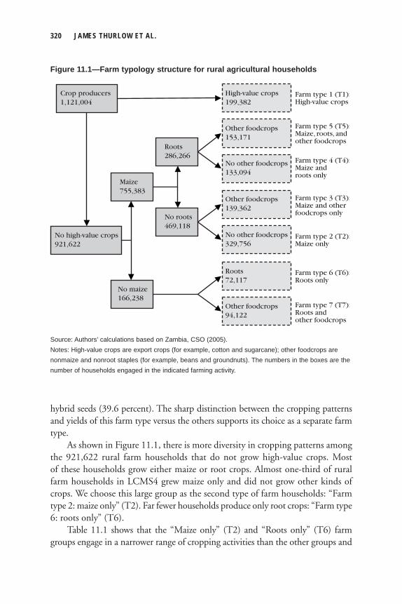
320 JAMES THURLOW ET AL.
hybrid seeds (39.6 percent). The sharp distinction between the cropping patterns and yields of this farm type versus the others supports its choice as a separate farm type.
As shown in Figure 11.1, there is more diversity in cropping patterns among the 921,622 rural farm households that do not grow high-value crops. Most of these households grow either maize or root crops. Almost one-third of rural farm households in LCMS4 grew maize only and did not grow other kinds of crops. We choose this large group as the second type of farm households: “Farm type 2: maize only” (T2). Far fewer households produce only root crops: “Farm type 6: roots only” (T6).
Table 11.1 shows that the “Maize only” (T2) and “Roots only” (T6) farm groups engage in a narrower range of cropping activities than the other groups and
Other foodcrops139,362
No other foodcrops329,756
Maize755,383
Roots286,266
No roots469,118
No high-value crops921,622
Other foodcrops153,171
No other foodcrops133,094
No maize166,238
Roots72,117
Other foodcrops94,122
Crop producers1,121,004
Farm type 5 (T5):Maize, roots, andother foodcrops
Farm type 4 (T4):Maize androots only
Farm type 3 (T3):Maize and otherfoodcrops only
Farm type 2 (T2):Maize only
Farm type 7 (T7):Roots andother foodcrops
Farm type 6 (T6):Roots only
Farm type 1 (T1):High-value crops
High-value crops199,382
Figure 11.1—Farm typology structure for rural agricultural households
Source: Authors’ calculations based on Zambia, CSO (2005).Notes: High-value crops are export crops (for example, cotton and sugarcane); other foodcrops are nonmaize and nonroot staples (for example, beans and groundnuts). The numbers in the boxes are the number of households engaged in the indicated farming activity.
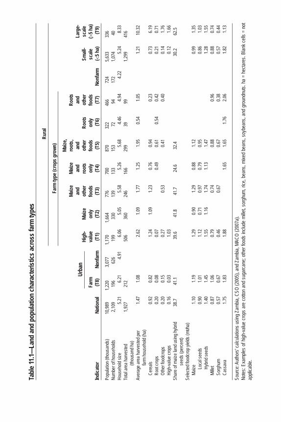
Tabl
e 11.1
—La
nd an
d po
pulat
ion
char
acte
ristic
s acr
oss f
arm
type
s
Rura
l
Fa
rm ty
pe (c
rops
gro
wn)
Maize
,
Ma
ize
Maize
ro
ots,
Ro
ots
and
and
and
an
d
La
rge-
High
- Ma
ize
othe
r ro
ots
othe
r Ro
ots
othe
r
Small
- sc
ale
Fa
rm
va
lue
only
food
s on
ly fo
ods
only
food
s
scale
(>
5 ha)
Indi
cato
r Na
tiona
l (T
8)
Nonf
arm
(T
1)
(T2)
(T
3)
(T4)
(T
5)
(T6)
(T
7)
Nonf
arm
(<
5 ha)
(
T9)
Popu
lation
(tho
usan
ds)
10,98
9 1,2
20
3,077
1,1
70
1,664
77
6 70
0 87
0 32
2 46
6 72
4 5,6
33
336
Numb
er of
hous
ehold
s 2,1
09
196
626
199
330
139
133
153
72
94
172
1,074
40
Hous
ehold
size
5.2
1 6.2
1 4.9
1 6.0
6 5.0
5 5.5
8 5.2
6 5.6
8 4.4
6 4.9
4 4.2
2 5.2
4 8.3
3To
tal ar
ea ha
rveste
d 1,9
27
212
50
6 36
0 24
6 16
6 29
9 39
99
1,299
41
6
(thou
sand
ha)
Aver
age a
rea h
arve
sted p
er
1.47
1.08
2.6
2 1.0
9 1.7
7 1.2
5 1.9
5 0.5
4 1.0
5
1.21
10.32
far
m ho
useh
old (h
a)
Ce
reals
0.9
2 0.8
2
1.24
1.09
1.23
0.76
0.94
0.2
3
0.73
6.19
Ro
ot cro
ps
0.20
0.08
0.0
7
0.4
9 0.6
1 0.5
4 0.4
2
0.21
0.71
Ot
her f
oodc
rops
0.2
0 0.1
5
0.27
0.5
3
0.41
0.4
0
0.14
1.76
Hi
gh-va
lue cr
ops
0.16
0.03
1.0
3
0.12
1.66
Shar
e of m
aize l
and u
sing h
ybrid
38
.7 41
.1
39.6
41.8
41.7
24.6
32.4
30
.2 62
.5
seed
s (pe
rcent)
Se
lected
food
crop y
ields
(mt/h
a)
Maize
1.1
0 1.1
9
1.29
0.90
1.29
0.88
1.12
0.9
9 1.3
5
Lo
cal s
eeds
0.9
0 1.0
1
1.12
0.71
0.97
0.79
0.95
0.8
6 1.0
3
Hy
brid
seed
s 1.4
0 1.4
5
1.55
1.16
1.74
1.13
1.47
1.2
8 1.5
5
Mille
t 0.8
7 1.0
6
0.79
0.7
4
0.88
0.9
6
0.88
0.74
So
rghu
m 0.5
7 0.6
7
0.46
0.6
7
0.67
0.3
8
0.57
0.44
Ca
ssav
a 1.7
5 1.8
3
1.88
1.65
1.65
1.76
2.06
1.8
2 1.1
3
Sour
ce: A
uthor
s’ ca
lculat
ions u
sing Z
ambia
, CSO
(200
5), a
nd Z
ambia
, MAC
O (2
007a
).No
tes: E
xamp
les o
f high
-value
crop
s are
cotto
n an
d su
garca
ne; o
ther f
oods
inclu
de m
illet,
sorg
hum,
rice
, bea
ns, m
ixed
bean
s, so
ybea
ns, a
nd g
roun
dnuts
. ha
= he
ctare
s. Bl
ank c
ells =
not
appli
cable
.
Urba
n
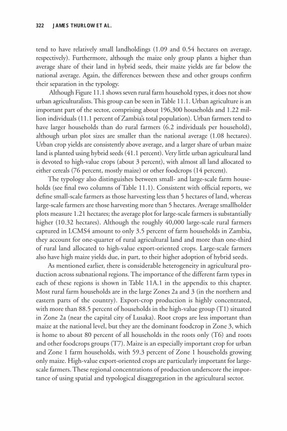
322 JAMES THURLOW ET AL.
tend to have relatively small landholdings (1.09 and 0.54 hectares on average, respectively). Furthermore, although the maize only group plants a higher than average share of their land in hybrid seeds, their maize yields are far below the national average. Again, the differences between these and other groups confi rm their separation in the typology.
Although Figure 11.1 shows seven rural farm household types, it does not show urban agriculturalists. This group can be seen in Table 11.1. Urban agriculture is an important part of the sector, comprising about 196,300 households and 1.22 mil-lion individuals (11.1 percent of Zambia’s total population). Urban farmers tend to have larger households than do rural farmers (6.2 individuals per household), although urban plot sizes are smaller than the national average (1.08 hectares). Urban crop yields are consistently above average, and a larger share of urban maize land is planted using hybrid seeds (41.1 percent). Very little urban agricultural land is devoted to high-value crops (about 3 percent), with almost all land allocated to either cereals (76 percent, mostly maize) or other foodcrops (14 percent).
The typology also distinguishes between small- and large-scale farm house-holds (see fi nal two columns of Table 11.1). Consistent with offi cial reports, we defi ne small-scale farmers as those harvesting less than 5 hectares of land, whereas large-scale farmers are those harvesting more than 5 hectares. Average smallholder plots measure 1.21 hectares; the average plot for large-scale farmers is substantially higher (10.32 hectares). Although the roughly 40,000 large-scale rural farmers captured in LCMS4 amount to only 3.5 percent of farm households in Zambia, they account for one-quarter of rural agricultural land and more than one-third of rural land allocated to high-value export-oriented crops. Large-scale farmers also have high maize yields due, in part, to their higher adoption of hybrid seeds.
As mentioned earlier, there is considerable heterogeneity in agricultural pro-duction across subnational regions. The importance of the different farm types in each of these regions is shown in Table 11A.1 in the appendix to this chapter. Most rural farm households are in the large Zones 2a and 3 (in the northern and eastern parts of the country). Export-crop production is highly concentrated, with more than 88.5 percent of households in the high-value group (T1) situated in Zone 2a (near the capital city of Lusaka). Root crops are less important than maize at the national level, but they are the dominant foodcrop in Zone 3, which is home to about 80 percent of all households in the roots only (T6) and roots and other foodcrops groups (T7). Maize is an especially important crop for urban and Zone 1 farm households, with 59.3 percent of Zone 1 households growing only maize. High-value export-oriented crops are particularly important for large-scale farmers. These regional concentrations of production underscore the impor-tance of using spatial and typological disaggregation in the agricultural sector.
ZAMBIA 323
The Zambian DCGE ModelThe DCGE model for Zambia includes 34 subsectors, half of which are in agricul-ture. A complete list of the sectors (and other accounts) is provided in Table 11A.2 in the appendix to this chapter, and the model’s specifi cation is described in Chapter 2 of this volume. In the Zambia model, agricultural production in rural areas is disaggregated according to the four agroecological zones. Although nonagricultural activities dominate the urban economy, agricultural production, particularly perish-able products supplying urban consumers, exists in urban areas. We therefore dis-aggregate two urban agricultural sectors, namely, metropolitan and other urban agriculture. Finally, crop production in each zone is further disaggregated into small- and large-scale farming groups. Information on crop production in each zone was drawn from LCMS4 (Zambia, CSO 2005).
The data used to calibrate the base year of the model are drawn from a variety of data sources. The core dataset underlying the DCGE model is a 2004 social accounting matrix (SAM) constructed for this study using information from nation-al accounts, trade data, and balance-of-payments information from the Central Statistical Offi ce (Zambia, CSO 2007a, 2007b). District-level agricultural produc-tion and price data were provided by the Ministry of Agriculture and Cooperatives (Zambia, MACO 2007a). When production information was unavailable for cer-tain crops (for example, horticulture), information was taken from FAO (2007). Agricultural production was fi rst disaggregated across regions by mapping districts to the four agroecological regions. Production was then disaggregated across farm types using information from the LCMS4 (Zambia, CSO 2005). The DCGE model is therefore consistent with offi cial agricultural production levels and yields at the zonal level, but it retains the within-region distribution of production cap-tured in the survey. Nonagricultural production and employment data were com-piled from LCMS4, national accounts, and World Bank (2010). On the demand side, information on industrial technologies (for example, intermediate and factor demand) was taken from an earlier SAM for Zambia (Thurlow, Robinson, and Evans 2005); the income and expenditure patterns for household groups are from LCMS4.
Baseline Growth ScenarioWe fi rst construct a baseline scenario for 2005–15 by drawing on recent production trends for individual subsectors (Zambia, CSO 2007a; Zambia, MACO 2007a). We assume that the nonagricultural subsectors maintain their long-term perfor-mance trends. However, in the baseline scenario, agricultural GDP grows at an average of 2.5 percent per year, which is slightly higher than what was observed
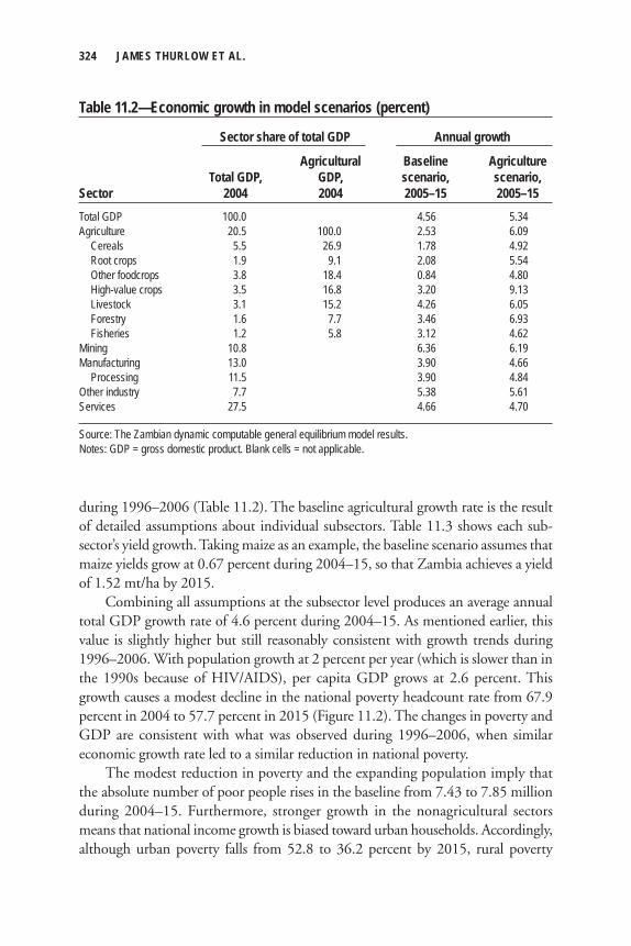
324 JAMES THURLOW ET AL.
during 1996–2006 (Table 11.2). The baseline agricultural growth rate is the result of detailed assumptions about individual subsectors. Table 11.3 shows each sub-sector’s yield growth. Taking maize as an example, the baseline scenario assumes that maize yields grow at 0.67 percent during 2004–15, so that Zambia achieves a yield of 1.52 mt/ha by 2015.
Combining all assumptions at the subsector level produces an average annual total GDP growth rate of 4.6 percent during 2004–15. As mentioned earlier, this value is slightly higher but still reasonably consistent with growth trends during 1996–2006. With population growth at 2 percent per year (which is slower than in the 1990s because of HIV/AIDS), per capita GDP grows at 2.6 percent. This growth causes a modest decline in the national poverty headcount rate from 67.9 percent in 2004 to 57.7 percent in 2015 (Figure 11.2). The changes in poverty and GDP are consistent with what was observed during 1996–2006, when similar economic growth rate led to a similar reduction in national poverty.
The modest reduction in poverty and the expanding population imply that the absolute number of poor people rises in the baseline from 7.43 to 7.85 million during 2004–15. Furthermore, stronger growth in the nonagricultural sectors means that national income growth is biased toward urban households. Accordingly, although urban poverty falls from 52.8 to 36.2 percent by 2015, rural poverty
Table 11.2—Economic growth in model scenarios (percent)
Sector share of total GDP Annual growth
Agricultural Baseline Agriculture Total GDP, GDP, scenario, scenario,Sector 2004 2004 2005–15 2005–15Total GDP 100.0 4.56 5.34Agriculture 20.5 100.0 2.53 6.09 Cereals 5.5 26.9 1.78 4.92 Root crops 1.9 9.1 2.08 5.54 Other foodcrops 3.8 18.4 0.84 4.80 High-value crops 3.5 16.8 3.20 9.13 Livestock 3.1 15.2 4.26 6.05 Forestry 1.6 7.7 3.46 6.93 Fisheries 1.2 5.8 3.12 4.62Mining 10.8 6.36 6.19Manufacturing 13.0 3.90 4.66 Processing 11.5 3.90 4.84Other industry 7.7 5.38 5.61Services 27.5 4.66 4.70
Source: The Zambian dynamic computable general equilibrium model results.Notes: GDP = gross domestic product. Blank cells = not applicable.
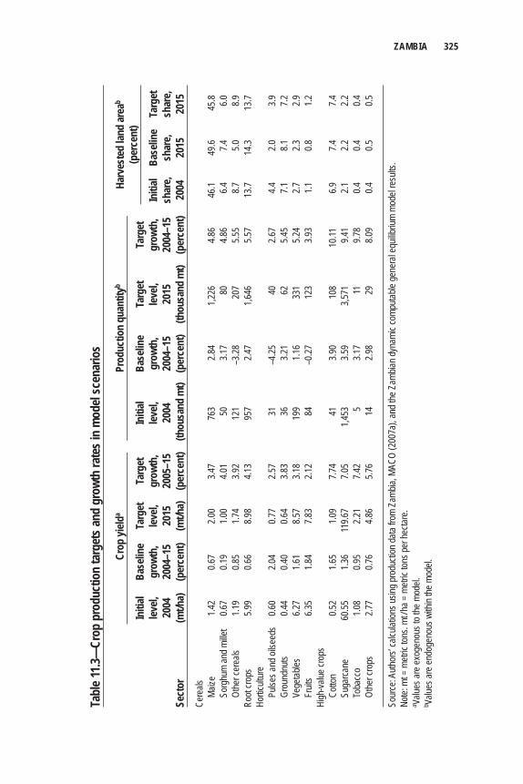
ZAMBIA 325
Tabl
e 11.3
—Cr
op p
rodu
ctio
n ta
rget
s and
gro
wth
rate
s in
mod
el sc
enar
ios
Cr
op yi
elda
Prod
uctio
n qu
antit
yb
In
itial
Base
line
Targ
et
Targ
et
Initi
al Ba
selin
e Ta
rget
Ta
rget
level,
gr
owth
, lev
el,
grow
th,
level,
gr
owth
, lev
el,
grow
th,
Initi
al Ba
selin
e Ta
rget
20
04
2004
–15
2015
20
05–1
5 20
04
2004
–15
2015
20
04–1
5 sh
are,
shar
e, sh
are,
Sect
or
(mt/h
a)
(per
cent
) (m
t/ha)
(p
erce
nt)
(tho
usan
d m
t) (p
erce
nt)
(thou
sand
mt)
(per
cent
) 20
04
2015
20
15Ce
reals
Maize
1.4
2 0.6
7 2.0
0 3.4
7 76
3 2.8
4 1,2
26
4.86
46.1
49.6
45.8
So
rghu
m an
d mille
t 0.6
7 0.1
9 1.0
0 4.0
1 50
3.1
7 80
4.8
6 6.4
7.4
6.0
Ot
her c
erea
ls
1.19
0.85
1.74
3.92
121
–3.28
20
7 5.5
5 8.7
5.0
8.9
Root
crops
5.9
9 0.6
6 8.9
8 4.1
3 95
7 2.4
7 1,6
46
5.57
13.7
14.3
13.7
Hortic
ultur
e
Pu
lses a
nd oi
lseed
s 0.6
0 2.0
4 0.7
7 2.5
7 31
–4
.25
40
2.67
4.4
2.0
3.9
Grou
ndnu
ts 0.4
4 0.4
0 0.6
4 3.8
3 36
3.2
1 62
5.4
5 7.1
8.1
7.2
Ve
getab
les
6.27
1.61
8.57
3.18
199
1.16
331
5.24
2.7
2.3
2.9
Fruit
s 6.3
5 1.8
4 7.8
3 2.1
2 84
–0
.27
123
3.93
1.1
0.8
1.2Hi
gh-va
lue cr
ops
Cotto
n 0.5
2 1.6
5 1.0
9 7.7
4 41
3.9
0 10
8 10
.11
6.9
7.4
7.4
Suga
rcane
60
.55
1.36
119.6
7 7.0
5 1,4
53
3.59
3,571
9.4
1 2.1
2.2
2.2
To
bacc
o 1.0
8 0.9
5 2.2
1 7.4
2 5
3.17
11
9.78
0.4
0.4
0.4
Othe
r cro
ps
2.77
0.76
4.86
5.76
14
2.98
29
8.09
0.4
0.5
0.5
Sour
ce: A
uthor
s’ ca
lculat
ions u
sing p
rodu
ction
data
from
Zamb
ia, M
ACO
(200
7a),
and t
he Z
ambia
n dyn
amic
comp
utable
gene
ral e
quilib
rium
mode
l resu
lts.
Note:
mt =
metr
ic ton
s. mt
/ ha =
metr
ic ton
s per
hecta
re.
a Value
s are
exog
enou
s to t
he m
odel.
b Value
s are
endo
geno
us w
ithin
the m
odel.
Harv
este
d lan
d ar
eab
(per
cent
)
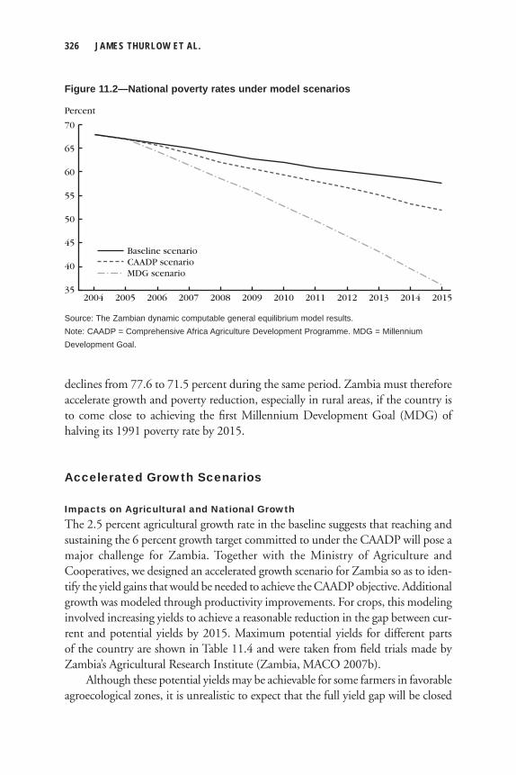
326 JAMES THURLOW ET AL.
declines from 77.6 to 71.5 percent during the same period. Zambia must therefore accelerate growth and poverty reduction, especially in rural areas, if the country is to come close to achieving the fi rst Millennium Development Goal (MDG) of halving its 1991 poverty rate by 2015.
Accelerated Growth Scenarios
Impacts on Agricultural and National GrowthThe 2.5 percent agricultural growth rate in the baseline suggests that reaching and sustaining the 6 percent growth target committed to under the CAADP will pose a major challenge for Zambia. Together with the Ministry of Agriculture and Cooperatives, we designed an accelerated growth scenario for Zambia so as to iden-tify the yield gains that would be needed to achieve the CAADP objective. Additional growth was modeled through productivity improvements. For crops, this modeling involved increasing yields to achieve a reasonable reduction in the gap between cur-rent and potential yields by 2015. Maximum potential yields for different parts of the country are shown in Table 11.4 and were taken from fi eld trials made by Zambia’s Agricultural Research Institute (Zambia, MACO 2007b).
Although these potential yields may be achievable for some farmers in favorable agroecological zones, it is unrealistic to expect that the full yield gap will be closed
Percent
70
Baseline scenario
35
65
60
55
50
45
40 CAADP scenarioMDG scenario
201520142013201220112010200920082007200620052004
Figure 11.2—National poverty rates under model scenarios
Source: The Zambian dynamic computable general equilibrium model results.Note: CAADP = Comprehensive Africa Agriculture Development Programme. MDG = Millennium Development Goal.
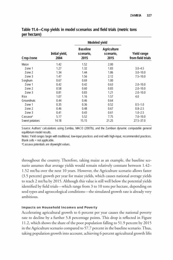
ZAMBIA 327
throughout the country. Therefore, taking maize as an example, the baseline sce-nario assumes that average yields would remain relatively constant between 1.42–1.52 mt/ha over the next 10 years. However, the Agriculture scenario allows faster (3.5 percent) growth per year for maize yields, which causes national average yields to reach 2 mt/ha by 2015. Although this value is still well below the potential yields identifi ed by fi eld trials—which range from 3 to 10 tons per hectare, depending on seed types and agroecological conditions—the simulated growth rate is already very ambitious.
Impacts on Household Incomes and Poverty Accelerating agricultural growth to 6 percent per year causes the national poverty rate to decline by a further 5.8 percentage points. This drop is refl ected in Figure 11.2, which shows the share of the poor population falling to 51.9 percent by 2015 in the Agriculture scenario compared to 57.7 percent in the baseline scenario. Thus, taking population growth into account, achieving 6 percent agricultural growth lifts
Table 11.4—Crop yields in model scenarios and field trials (metric tons per hectare)
Modeled yield
Baseline Agriculture Initial yield, scenario, scenario, Yield rangeCrop / zone 2004 2015 2015 from field trialsMaize 1.42 1.52 2.00 Zone 1 1.27 1.32 1.83 3.0–4.5 Zone 2 1.34 1.44 1.86 3.0–10.0 Zone 3 1.47 1.56 2.12 7.5–10.0Sorghum 0.67 0.69 1.00 Zone 1 0.42 0.42 0.63 2.0–10.0 Zone 2 0.58 0.60 0.83 2.0–10.0 Zone 3 0.81 0.83 1.21 2.0–10.0Rice 1.07 1.16 1.57 4.0Groundnuts 0.44 0.46 0.64 Zone 1 0.35 0.36 0.52 0.5–1.0 Zone 2 0.46 0.48 0.67 0.8–2.5 Zone 3 0.41 0.43 0.61 1.0–2.5Cassavaa 5.17 5.52 7.75 7.0–10.0 Sweet potatoes 14.18 15.15 21.25 27.5–37.0
Source: Authors’ calculations using Zambia, MACO (2007b), and the Zambian dynamic computable general equilibrium model results.Notes: Yield ranges begin with traditional, low-input practices and end with high-input, recommended practices. Blank cells = not applicable. aCassava potentials are dryweight values.
328 JAMES THURLOW ET AL.
an additional 780,000 people above the poverty line by 2015, and it is suffi cient to reverse current trends by reducing the absolute number of poor people in Zambia. Food security would also improve, with annual average per capita cereal consump-tion rising from 81.2 kilograms in 2015 in the baseline and to 93.1 kilograms in the Agriculture scenario. Finally, although Zambia’s dependence on imported cereals is not eliminated, accelerating agricultural growth greatly reduces the country’s trade defi cit for foodcrops.
Not all households will benefi t equally when crop yields and subsector growth rates increase in the Agriculture scenario. Larger-scale and urban farms benefi t more from additional maize and high-value crop production in this scenario, because high-value crops are typically grown on large-scale farms and maize is a particularly important crop for urban households. This result can be seen in Figure 11.3, which shows the contribution of growth in different subsectors to changes in the value of production. The fi gure highlights the importance of growth led by export crops in determining production growth for certain farm types. Export crops generate one-third of additional production at the national level and most of the production growth for farmers growing high-value crops (groups T1 and T9).
With the exception of export-crop producers, most small-scale farms benefi t equally in the Agriculture scenario. However, despite this even distribution of bene-fi ts, Figure 11.3 indicates that the sources of additional production vary dramatically across smallholder farm types. Not surprisingly, households that are more dependent on maize and root crops tend to benefi t more from growth driven by cereals and root crops, respectively. However, there are two forces driving changes in overall production: direct and indirect effects of subsector-specifi c yield improvements. Increasing yield has a direct effect on farm incomes, because it increases the quantity of output that a farm household can produce using the same quantity of factor inputs. However, increased production faces demand and market constraints, as prices typi-cally fall following increases in yields. Thus, the direct impact of crop-yield improve-ments for a specifi c farm household is its net effect on crop production weighted by the share of the household’s land allocated to producing that crop. This direct effect therefore assumes that land allocations remain fi xed. However, farmers may reallocate land in response to changes in relative prices, meaning that the indirect impact of crop-yield improvement is the potentially positive impact of reallocating land to other crops. The DCGE model captures both direct and the indirect effects.
Table 11.5 shows changes in household incomes and poverty rates for different farm types and household groups. Small-scale rural farmers benefi t by at least as much as urban households in the Agriculture scenario. Per capita household incomes for rural households grow by an additional 2.2 percentage points per year compared to 1.95 percentage points for urban households (see Table 11.5). This increase is also refl ected in changes in poverty; rural poverty declines by an additional 6.4 percent-
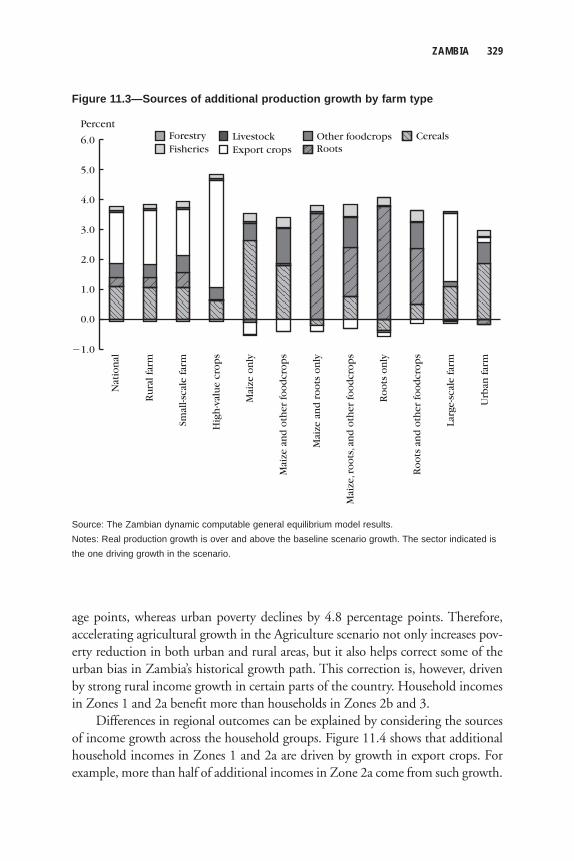
ZAMBIA 329
age points, whereas urban poverty declines by 4.8 percentage points. Therefore, accelerating agricultural growth in the Agriculture scenario not only increases pov-erty reduction in both urban and rural areas, but it also helps correct some of the urban bias in Zambia’s historical growth path. This correction is, however, driven by strong rural income growth in certain parts of the country. Household incomes in Zones 1 and 2a benefi t more than households in Zones 2b and 3.
Differences in regional outcomes can be explained by considering the sources of income growth across the household groups. Figure 11.4 shows that additional household incomes in Zones 1 and 2a are driven by growth in export crops. For example, more than half of additional incomes in Zone 2a come from such growth.
Percent
�1.0
6.0
5.0
4.0
3.0
0.0
2.0
1.0
Nat
ion
al
Ru
ral f
arm
Mai
ze o
nly
Mai
ze a
nd
oth
er f
oo
dcr
op
s
Mai
ze a
nd
ro
ots
on
ly
Smal
l-sca
le f
arm
Hig
h-v
alu
e cr
op
s
Mai
ze, r
oo
ts, a
nd
oth
er f
oo
dcr
op
s
Ro
ots
on
ly
Ro
ots
an
d o
ther
fo
od
cro
ps
Lar
ge-s
cale
far
m
Urb
an f
arm
Other foodcropsFisheriesForestry
Export cropsLivestock Cereals
Roots
Figure 11.3—Sources of additional production growth by farm type
Source: The Zambian dynamic computable general equilibrium model results.Notes: Real production growth is over and above the baseline scenario growth. The sector indicated is the one driving growth in the scenario.
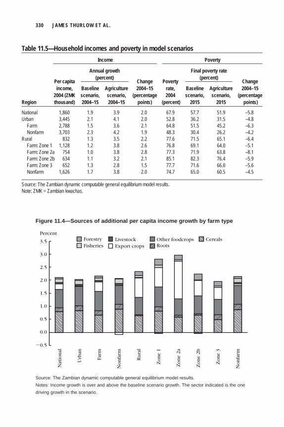
330 JAMES THURLOW ET AL.
Table 11.5—Household incomes and poverty in model scenarios Income Poverty
Per capita Change Poverty Change income, Baseline Agriculture 2004–15 rate, Baseline Agriculture 2004–15 2004 (ZMK scenario, scenario, (percentage 2004 scenario, scenario, (percentageRegion thousand) 2004–15 2004–15 points) (percent) 2015 2015 points)
National 1,860 1.9 3.9 2.0 67.9 57.7 51.9 –5.8Urban 3,445 2.1 4.1 2.0 52.8 36.2 31.5 –4.8 Farm 2,788 1.5 3.6 2.1 64.8 51.5 45.2 –6.3 Nonfarm 3,703 2.3 4.2 1.9 48.3 30.4 26.2 –4.2Rural 832 1.3 3.5 2.2 77.6 71.5 65.1 –6.4 Farm: Zone 1 1,128 1.2 3.8 2.6 76.8 69.1 64.0 –5.1 Farm: Zone 2a 754 1.0 3.8 2.8 77.3 71.9 63.8 –8.1 Farm: Zone 2b 634 1.1 3.2 2.1 85.1 82.3 76.4 –5.9 Farm: Zone 3 652 1.3 2.8 1.5 77.7 71.6 66.0 –5.6 Nonfarm 1,626 1.7 3.8 2.0 74.7 65.0 60.5 –4.5
Source: The Zambian dynamic computable general equilibrium model results.Note: ZMK = Zambian kwachas.
Annual growth (percent)
Final poverty rate(percent)
Percent
�0.5
3.5
2.5
3.0
2.0
1.5
0.0
1.0
0.5
Nat
ion
al
Urb
an
Ru
ral
Zo
ne
1
Zo
ne
2a
Farm
No
nfa
rm
Zo
ne
2b
Zo
ne
3
No
nfa
rmOther foodcrops
FisheriesForestry
Export cropsLivestock Cereals
Roots
Figure 11.4—Sources of additional per capita income growth by farm type
Source: The Zambian dynamic computable general equilibrium model results.Notes: Income growth is over and above the baseline scenario growth. The sector indicated is the one driving growth in the scenario.
ZAMBIA 331
This is because households in these southern zones have better access to markets, major transport routes, and urban centers; they are thus better positioned to benefi t from export-led growth. In contrast, households in northern Zone 3 benefi t more from growth in root crops, which is not surprising, given the importance of these crops for farmers in this region.
Overall, the model results indicate that it is possible for Zambia to reach the CAADP target of 6 percent agricultural growth per year. However, given the current poor performance of the agricultural sector, achieving that growth target will require additional growth in all crops and subsectors. Thus, Zambia cannot rely on only maize or high-value export crops to achieve the aggregate agricultural growth targets. If the above-described crop- and subsector-level targets can be achieved, then the resulting broader-based agricultural growth is likely to benefi t households in both rural and urban areas. However, the high growth potential of specifi c export crops and better market conditions in certain parts of the country may cause uneven income growth and poverty reduction.
Subsector Growth Contributions to Poverty ReductionThe above fi ndings highlight the potential contributions of different crops and subsectors in increasing agricultural growth and reducing poverty. However, the different sizes of these subsectors make it diffi cult to compare the effectiveness of sectoral growth in reducing poverty. Understanding how poverty–growth linkages vary at the subsector and household levels is important for designing pro-poor growth strategies. Hence, we calculate poverty–growth elasticities that allow us to compare the pro-poorness of growth driven by different subsectors. These elasticities are endogenous outcomes of the model. Each scenario allows productivity growth to occur only for a specifi c group of crops or subsectors. We increase productivity in these sectors to achieve the same absolute increase in total GDP as in the Agriculture scenario. Thus, small sectors have to grow faster than larger ones to achieve the same effect on national GDP. However, even though the growth effect is the same for each crop, the effect on poverty can be different because of economy-wide linkages and the heterogeneity of income sources across household groups. For example, some households may have better opportunities to produce high-value export commodities and are thus better positioned to benefi t from export agricul-ture. However, households producing export crops are often less poor than other rural households. Thus, agricultural growth driven by export crops may have less impact on poverty, especially among the poorest households. In contrast, foodcrops tend to be a more important source of agricultural incomes for poorer households in more remote areas of the country. Thus, growth in foodcrops is expected to be more effective at reducing poverty than is similar growth in export crops.
The poverty–growth elasticity used in this study measures the responsiveness of the poverty rate to changes in per capita agricultural GDP growth. Table 11.6
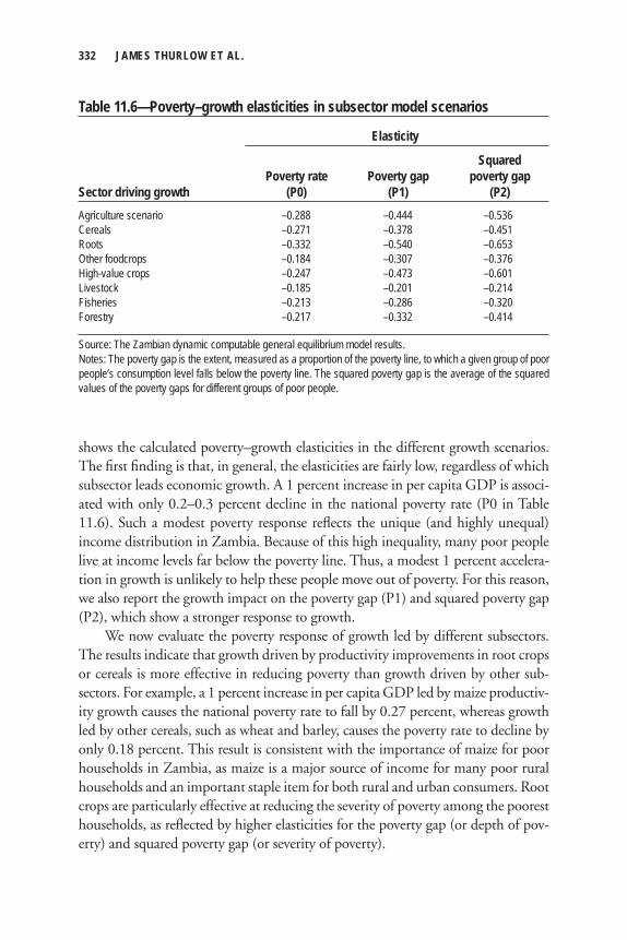
332 JAMES THURLOW ET AL.
shows the calculated poverty–growth elasticities in the different growth scenarios. The fi rst fi nding is that, in general, the elasticities are fairly low, regardless of which subsector leads economic growth. A 1 percent increase in per capita GDP is associ-ated with only 0.2–0.3 percent decline in the national poverty rate (P0 in Table 11.6). Such a modest poverty response refl ects the unique (and highly unequal) income distribution in Zambia. Because of this high inequality, many poor people live at income levels far below the poverty line. Thus, a modest 1 percent accelera-tion in growth is unlikely to help these people move out of poverty. For this reason, we also report the growth impact on the poverty gap (P1) and squared poverty gap (P2), which show a stronger response to growth.
We now evaluate the poverty response of growth led by different subsectors. The results indicate that growth driven by productivity improvements in root crops or cereals is more effective in reducing poverty than growth driven by other sub-sectors. For example, a 1 percent increase in per capita GDP led by maize productiv-ity growth causes the national poverty rate to fall by 0.27 percent, whereas growth led by other cereals, such as wheat and barley, causes the poverty rate to decline by only 0.18 percent. This result is consistent with the importance of maize for poor households in Zambia, as maize is a major source of income for many poor rural households and an important staple item for both rural and urban consumers. Root crops are particularly effective at reducing the severity of poverty among the poorest households, as refl ected by higher elasticities for the poverty gap (or depth of pov-erty) and squared poverty gap (or severity of poverty).
Table 11.6—Poverty–growth elasticities in subsector model scenarios
Elasticity
Squared Poverty rate Poverty gap poverty gapSector driving growth (P0) (P1) (P2)Agriculture scenario –0.288 –0.444 –0.536Cereals –0.271 –0.378 –0.451Roots –0.332 –0.540 –0.653Other foodcrops –0.184 –0.307 –0.376High-value crops –0.247 –0.473 –0.601Livestock –0.185 –0.201 –0.214Fisheries –0.213 –0.286 –0.320Forestry –0.217 –0.332 –0.414
Source: The Zambian dynamic computable general equilibrium model results.Notes: The poverty gap is the extent, measured as a proportion of the poverty line, to which a given group of poor people’s consumption level falls below the poverty line. The squared poverty gap is the average of the squared values of the poverty gaps for different groups of poor people.
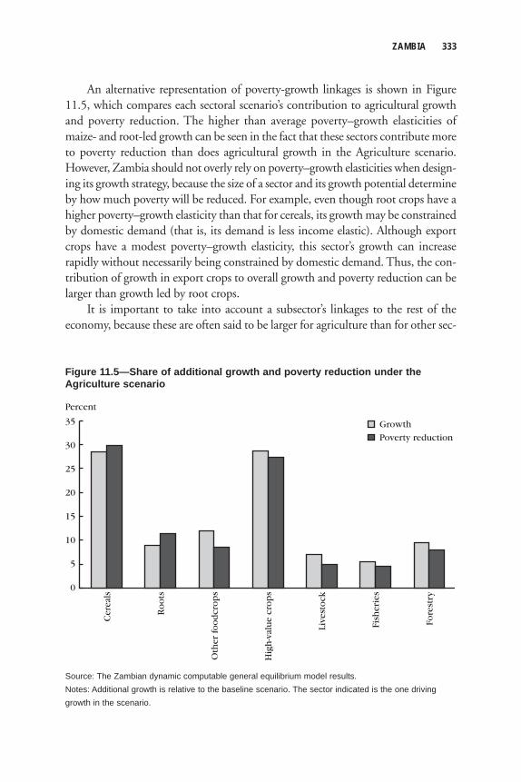
ZAMBIA 333
An alternative representation of poverty-growth linkages is shown in Figure 11.5, which compares each sectoral scenario’s contribution to agricultural growth and poverty reduction. The higher than average poverty–growth elasticities of maize- and root-led growth can be seen in the fact that these sectors contribute more to poverty reduction than does agricultural growth in the Agriculture scenario. However, Zambia should not overly rely on poverty–growth elasticities when design-ing its growth strategy, because the size of a sector and its growth potential determine by how much poverty will be reduced. For example, even though root crops have a higher poverty–growth elasticity than that for cereals, its growth may be constrained by domestic demand (that is, its demand is less income elastic). Although export crops have a modest poverty–growth elasticity, this sector’s growth can increase rapidly without necessarily being constrained by domestic demand. Thus, the con-tribution of growth in export crops to overall growth and poverty reduction can be larger than growth led by root crops.
It is important to take into account a subsector’s linkages to the rest of the economy, because these are often said to be larger for agriculture than for other sec-
Cer
eals
Ro
ots
Live
sto
ck
Fish
erie
s
Oth
er f
oo
dcr
op
s
Hig
h-v
alu
e cr
op
s
Fore
stry
Poverty reduction
Growth
Percent
35
0
30
25
20
15
10
5
Figure 11.5—Share of additional growth and poverty reduction under the Agriculture scenario
Source: The Zambian dynamic computable general equilibrium model results.Notes: Additional growth is relative to the baseline scenario. The sector indicated is the one driving growth in the scenario.
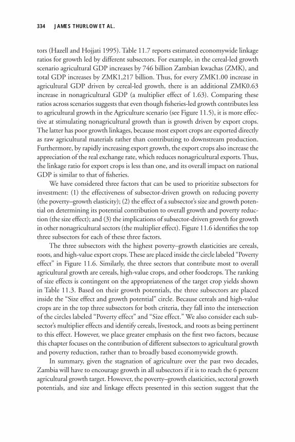
334 JAMES THURLOW ET AL.
tors (Hazell and Hojjati 1995). Table 11.7 reports estimated economywide linkage ratios for growth led by different subsectors. For example, in the cereal-led growth scenario agricultural GDP increases by 746 billion Zambian kwachas (ZMK), and total GDP increases by ZMK1,217 billion. Thus, for every ZMK1.00 increase in agricultural GDP driven by cereal-led growth, there is an additional ZMK0.63 increase in nonagricultural GDP (a multiplier effect of 1.63). Comparing these ratios across scenarios suggests that even though fi sheries-led growth contributes less to agricultural growth in the Agriculture scenario (see Figure 11.5), it is more effec-tive at stimulating nonagricultural growth than is growth driven by export crops. The latter has poor growth linkages, because most export crops are exported directly as raw agricultural materials rather than contributing to downstream production. Furthermore, by rapidly increasing export growth, the export crops also increase the appreciation of the real exchange rate, which reduces nonagricultural exports. Thus, the linkage ratio for export crops is less than one, and its overall impact on national GDP is similar to that of fi sheries.
We have considered three factors that can be used to prioritize subsectors for investment: (1) the effectiveness of subsector-driven growth on reducing poverty (the poverty–growth elasticity); (2) the effect of a subsector’s size and growth poten-tial on determining its potential contribution to overall growth and poverty reduc-tion (the size effect); and (3) the implications of subsector-driven growth for growth in other nonagricultural sectors (the multiplier effect). Figure 11.6 identifi es the top three subsectors for each of these three factors.
The three subsectors with the highest poverty–growth elasticities are cereals, roots, and high-value export crops. These are placed inside the circle labeled “Poverty effect” in Figure 11.6. Similarly, the three sectors that contribute most to overall agricultural growth are cereals, high-value crops, and other foodcrops. The ranking of size effects is contingent on the appropriateness of the target crop yields shown in Table 11.3. Based on their growth potentials, the three subsectors are placed inside the “Size effect and growth potential” circle. Because cereals and high-value crops are in the top three subsectors for both criteria, they fall into the intersection of the circles labeled “Poverty effect” and “Size effect.” We also consider each sub-sector’s multiplier effects and identify cereals, livestock, and roots as being pertinent to this effect. However, we place greater emphasis on the fi rst two factors, because this chapter focuses on the contribution of different subsectors to agricultural growth and poverty reduction, rather than to broadly based economywide growth.
In summary, given the stagnation of agriculture over the past two decades, Zambia will have to encourage growth in all subsectors if it is to reach the 6 percent agricultural growth target. However, the poverty–growth elasticities, sectoral growth potentials, and size and linkage effects presented in this section suggest that the
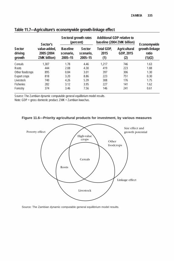
ZAMBIA 335
Table 11.7—Agriculture’s economywide growth-linkage effect
Sector’s EconomywideSector value-added, Baseline Sector Total GDP, Agricultural growth-linkagedriving 2005 (2004 scenario, scenario, 2015 GDP, 2015 ratiogrowth ZMK billion) 2005–15 2005–15 (1) (2) (1)/(2) Cereals 1,307 1.78 4.46 1,217 746 1.63Roots 444 2.08 4.30 419 223 1.88Other foodcrops 895 0.84 3.01 397 306 1.30Export crops 818 3.20 8.86 223 751 0.30Livestock 740 4.26 5.39 308 176 1.75Fisheries 282 3.12 3.95 227 141 1.62Forestry 374 3.46 7.56 146 241 0.61
Source: The Zambian dynamic computable general equilibrium model results.Note: GDP = gross domestic product. ZMK = Zambian kwachas.
Sectoral growth rates (percent)
Additional GDP relative to baseline (2004 ZMK billion)
Poverty effectSize effect andgrowth potential
Otherfoodcrops
Cereals
High-valuecrops
Roots
Linkage effect
Livestock
Figure 11.6—Priority agricultural products for investment, by various measures
Source: The Zambian dynamic computable general equilibrium model results.
336 JAMES THURLOW ET AL.
highest priority should be given to improving cereal yields and encouraging high-value export crops.
Agricultural Investment Analysis
Baseline Investment ScenarioTo promote agricultural growth and poverty reduction in Zambia in general, the Government of Zambia has already implemented a number of agricultural develop-ment programs. For example, the government’s Fifth National Development Plan for 2006–10 included plans to invest ZMK4,069 billion in R&D and extension, markets, rural infrastructure, human and natural resource development, livestock, and fi sheries. Because of a lack of Zambia-specifi c data needed to estimate the return on different types of public investment, we use the procedure outlined in Chapter 2. Specifi cally, we estimate the aggregate public agricultural expenditure (PAE) required to reach the 6 percent growth target. Simple univariate regression analysis of agricultural GDP on total agricultural expenditures using national historical data gives similar trends for Malawi and Zambia, and so we used the same range of elasticities for Zambia as used for Malawi. The elasticities of agricultural GDP with respect to aggregate PAE are 0.15 and 0.30, representing less and more optimistic public effi ciency scenarios, respectively. The parameter values used in public invest-ment simulations are summarized in Table 11A.3 in the appendix to this chapter.
Three scenarios are simulated over 2004–15 that estimate the required PAE. The fi rst is a baseline, in which we assume that PAE and public nonagricultural spending (PNE) continue to grow according to 1992–2006 trends (an annual aver-age real growth rate of 8.4 and 2.3 percent per year, respectively). We also use the 1992–2006 annual average government expenditures of ZMK200 billion and ZMK4,983 billion in 2004 as benchmarks for PAE and PNE, respectively. Baseline results reveal that the share of PAE in total expenditure rises from 3.9 percent in 2004 to 5.4 percent in 2010 and 7.1 percent in 2015 (Table 11.8). This is because recent PAE grows more rapidly than total spending does. However, the share of PAE in total spending will still remain below the 10 percent target proposed by the CAADP. The growth and associated poverty-reduction targets are therefore beyond reach in this business-as-usual scenario, which is not surprising, given Zambia’s poor historical performance.
Investment Needed to Meet the CAADP TargetThe two remaining investment scenarios assess the additional PAE required to support a 6 percent agricultural growth target. The fi rst scenario assumes that agri-cultural GDP growth is supported by an increase in PAE alone—all other factors
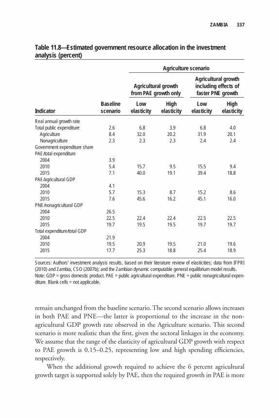
ZAMBIA 337
remain unchanged from the baseline scenario. The second scenario allows increases in both PAE and PNE—the latter is proportional to the increase in the non-agricultural GDP growth rate observed in the Agriculture scenario. This second scenario is more realistic than the fi rst, given the sectoral linkages in the economy. We assume that the range of the elasticity of agricultural GDP growth with respect to PAE growth is 0.15–0.25, representing low and high spending effi ciencies, respectively.
When the additional growth required to achieve the 6 percent agricultural growth target is supported solely by PAE, then the required growth in PAE is more
Table 11.8—Estimated government resource allocation in the investment analysis (percent)
Agriculture scenario
Agricultural growth Agricultural growth including effects of from PAE growth only faster PNE growth
Baseline Low High Low HighIndicator scenario elasticity elasticity elasticity elasticityReal annual growth rateTotal public expenditure 2.6 6.8 3.9 6.8 4.0 Agriculture 8.4 32.0 20.2 31.9 20.1 Nonagriculture 2.3 2.3 2.3 2.4 2.4Government expenditure sharePAE/total expenditure 2004 3.9 2010 5.4 15.7 9.5 15.5 9.4 2015 7.1 40.0 19.1 39.4 18.8PAE/agricultural GDP 2004 4.1 2010 5.7 15.3 8.7 15.2 8.6 2015 7.6 45.6 16.2 45.1 16.0PNE/nonagricultural GDP 2004 26.5 2010 22.5 22.4 22.4 22.5 22.5 2015 19.7 19.5 19.5 19.7 19.7Total expenditure/total GDP 2004 21.9 2010 19.5 20.9 19.5 21.0 19.6 2015 17.7 25.3 18.8 25.4 18.9
Sources: Authors’ investment analysis results, based on their literature review of elasticities; data from IFPRI (2010) and Zambia, CSO (2007b); and the Zambian dynamic computable general equilibrium model results. Note: GDP = gross domestic product. PAE = public agricultural expenditure. PNE = public nonagricultural expen-diture. Blank cells = not applicable.
338 JAMES THURLOW ET AL.
than 20 percent per year, even in the high elasticity (better effi ciency) scenario (see Table 11.8). It is as high as 32 percent with a low elasticity. Assuming that the gov-ernment’s allocation to PNE continues to grow at the baseline rate, then the total budget is estimated to grow at 3.9 and 6.8 percent per year in high and low effi -ciency scenarios, respectively. Again, with PAE growing more rapidly than total spending, the PAE share rises to 19.1–40.0 percent by 2015. Increasing PNE growth in the second scenario makes little difference, because additional non-agricultural GDP growth in the Agriculture scenario is very small. The investment analysis shows that if 6 percent agricultural growth is to be achieved, the Government of Zambia will need to allocate at least one-fi fth of its total budget to agriculture by 2015. This number assumes that the government achieves a higher effi ciency in its spending. A key element in improving public spending effi ciency is identifying appropriate investments.
Identifying Investment PrioritiesIdentifying investment priorities is challenging because of data and information constraints on the performance of specifi c investment programs. The recent study by Nin Pratt and Yu (2008) shows that total factor productivity growth during 1994–2003 in Zambia (0.03 percent annual average) is one of the lowest in Africa and is characterized by virtually stagnant or declining growth in all factors of pro-duction, including fertilizers, tractors, livestock, and labor.
As in many other African countries, the Government of Zambia has been subsidizing fertilizers used by farmers. Nearly 40 percent of the resources earmarked for the agricultural sector have been spent on the Fertilizer Support Program and the operations of the Food Reserve Agency, both of which directly support the maize subsector (Govereh et al. 2006). For example, the 2001/02 postharvest survey indi-cates that 99 percent of the inorganic fertilizers used in Zambia were applied to maize. The results of our poverty–growth analysis presented earlier show that focus-ing investment on a single subsector is unlikely to produce broadly based poverty reduction. The DCGE model analysis also showed that roots and export crops are important subsectors for accelerating growth and poverty reduction, especially in the northern parts of the country, where poverty is most severe. Thus, although we are unable to assess the impact of agricultural spending on raising yields and growth in the individual subsectors, our analysis indicates the need for a more balanced spending portfolio.
To increase agricultural production, reduce production costs, and protect the environment by employing sustainable agricultural production, Zambian farmers need improved technologies capable of helping them increase yields, manage water, and use natural resources in a more sustainable manner while still being profi table under local farming and market conditions. A key investment area to support such
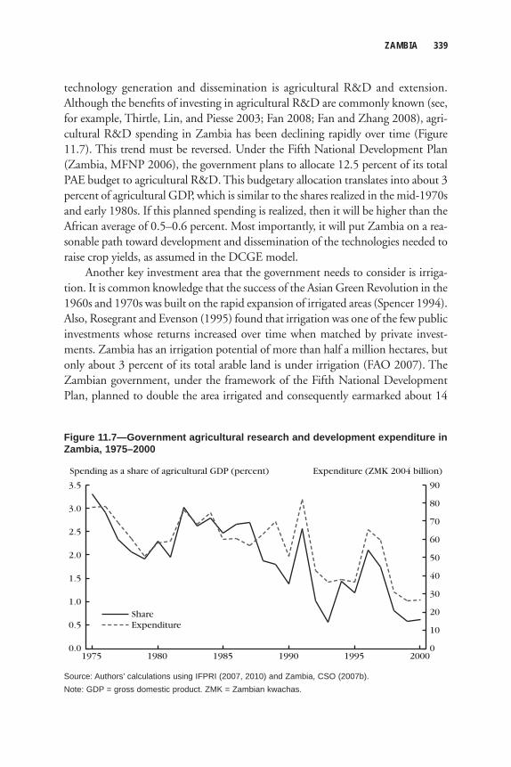
ZAMBIA 339
technology generation and dissemination is agricultural R&D and extension. Although the benefi ts of investing in agricultural R&D are commonly known (see, for example, Thirtle, Lin, and Piesse 2003; Fan 2008; Fan and Zhang 2008), agri-cultural R&D spending in Zambia has been declining rapidly over time (Figure 11.7). This trend must be reversed. Under the Fifth National Development Plan (Zambia, MFNP 2006), the government plans to allocate 12.5 percent of its total PAE budget to agricultural R&D. This budgetary allocation translates into about 3 percent of agricultural GDP, which is similar to the shares realized in the mid-1970s and early 1980s. If this planned spending is realized, then it will be higher than the African average of 0.5–0.6 percent. Most importantly, it will put Zambia on a rea-sonable path toward development and dissemination of the technologies needed to raise crop yields, as assumed in the DCGE model.
Another key investment area that the government needs to consider is irriga-tion. It is common knowledge that the success of the Asian Green Revolution in the 1960s and 1970s was built on the rapid expansion of irrigated areas (Spencer 1994). Also, Rosegrant and Evenson (1995) found that irrigation was one of the few public investments whose returns increased over time when matched by private invest-ments. Zambia has an irrigation potential of more than half a million hectares, but only about 3 percent of its total arable land is under irrigation (FAO 2007). The Zambian government, under the framework of the Fifth National Development Plan, planned to double the area irrigated and consequently earmarked about 14
Spending as a share of agricultural GDP (percent) Expenditure (ZMK 2004 billion)
3.5
0.0
3.0
2.5
ShareExpenditure
200019951990198519801975
2.0
1.5
1.0
0.5
90
0
80
70
60
50
40
30
20
10
Figure 11.7—Government agricultural research and development expenditure in Zambia, 1975–2000
Source: Authors’ calculations using IFPRI (2007, 2010) and Zambia, CSO (2007b).Note: GDP = gross domestic product. ZMK = Zambian kwachas.
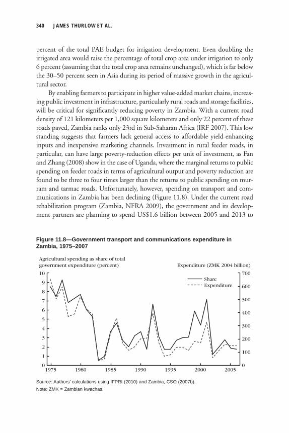
340 JAMES THURLOW ET AL.
percent of the total PAE budget for irrigation development. Even doubling the irrigated area would raise the percentage of total crop area under irrigation to only 6 percent (assuming that the total crop area remains unchanged), which is far below the 30–50 percent seen in Asia during its period of massive growth in the agricul-tural sector.
By enabling farmers to participate in higher value-added market chains, increas-ing public investment in infrastructure, particularly rural roads and storage facilities, will be critical for signifi cantly reducing poverty in Zambia. With a current road density of 121 kilometers per 1,000 square kilometers and only 22 percent of these roads paved, Zambia ranks only 23rd in Sub-Saharan Africa (IRF 2007). This low standing suggests that farmers lack general access to affordable yield-enhancing inputs and inexpensive marketing channels. Investment in rural feeder roads, in particular, can have large poverty-reduction effects per unit of investment, as Fan and Zhang (2008) show in the case of Uganda, where the marginal returns to public spending on feeder roads in terms of agricultural output and poverty reduction are found to be three to four times larger than the returns to public spending on mur-ram and tarmac roads. Unfortunately, however, spending on transport and com-munications in Zambia has been declining (Figure 11.8). Under the current road rehabilitation program (Zambia, NFRA 2009), the government and its develop-ment partners are planning to spend US$1.6 billion between 2005 and 2013 to
Agricultural spending as share of totalgovernment expenditure (percent) Expenditure (ZMK 2004 billion)
10
0
6
5
ShareExpenditure
200519951990198519801975
4
9
8
7
3
2
1
700
0
600
500
400
300
200
100
2000
Figure 11.8—Government transport and communications expenditure in Zambia, 1975–2007
Source: Authors’ calculations using IFPRI (2010) and Zambia, CSO (2007b).Note: ZMK = Zambian kwachas.
ZAMBIA 341
improve the road network. The main objective of the program is to rehabilitate the existing network, meaning that the road density will still remain low. However, road conditions are likely to improve signifi cantly. New roads must be built, especially to improve the market integration of Zone 3, where large growth and poverty-reduction potentials have been identifi ed.
ConclusionsThe DCGE model results indicate that Zambia would need to achieve quite ambi-tious improvements in crop yields and subsector growth if it is to achieve the CAADP target of 6 percent agricultural growth by 2015. If attained, this fast growth would lift an additional 780,000 people above the poverty line by 2015. It would not, however, be suffi cient for Zambia to achieve the fi rst MDG of halving national poverty.
Most households are expected to benefi t from faster agricultural growth, and the distribution of additional incomes becomes more even. However, farm house-holds growing high-value export crops stand to gain more than those relying more on foodcrops or livestock. Furthermore, households in agroecological Zones 1 and 2a in the southern parts of the country benefi t more than households in more remote zones. Finally, although rural households benefi t more than urban house-holds, not least because the former are more dependent on agricultural incomes, urban households also benefi t. This is because urban agriculturalists make up a signifi cant share of agricultural producers in Zambia, and agricultural commodities are an important part of urban consumer baskets.
Comparing the effectiveness of growth driven by different subsectors on reducing poverty and encouraging broadly based growth, we fi nd that 1 percent GDP growth driven by either cereals or root crops leads to considerably more poverty reduction than similar growth in export crops. This is because yield improvements in the former crops not only benefi t households directly by increas-ing incomes from cereals and root-crop production but also indirectly by allowing farmers to diversify their land allocations to high-value crops. The benefi ts of diversifi cation from promoting maize has been confi rmed by empirical studies for Zambia (see, for example, Zulu et al. 2000; Phiri et al. 2004). Foodcrops also have stronger growth linkages to nonagricultural sectors, thereby stimulating economy-wide growth and poverty reduction. However, the high growth potential of export crops relative to that of foodcrops means that export-led growth may still account for a large share of poverty reduction. Furthermore, the small initial size and geographic concentration of certain foodcrops, such as roots, means that their potential contribution to national growth and poverty reduction may be limited, at least over the short term. Taken together, our fi ndings highlight the importance
342 JAMES THURLOW ET AL.
of broadly based agricultural growth, but they accord a high priority to maize, roots, and smallholder export crops.
Finally, it is crucial that the Government of Zambia increase both the level and effi ciency of its spending in the agricultural sector. The latter includes reforming public institutions, particularly those with any agriculture-related functions, to improve the provision and delivery of agricultural public goods and services. Our analysis indicates that total public spending on agriculture would have to grow by at least 20 percent per year to achieve and sustain 6 percent agricultural growth. Thus, the government would need to allocate at least one-fi fth of its total budget to agriculture. Without this heightened level of commitment to agriculture, Zambia will further entrench its historical performance of achieving economic growth with-out reducing poverty.
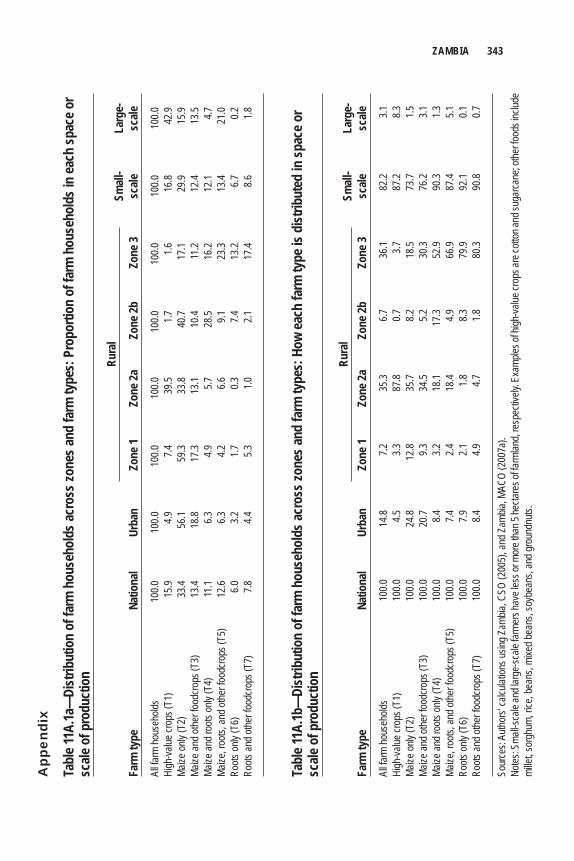
ZAMBIA 343Ta
ble 1
1A.1a
—Di
strib
utio
n of
farm
hou
seho
lds a
cros
s zon
es an
d fa
rm ty
pes:
Pro
porti
on o
f far
m h
ouse
hold
s in
each
spac
e or
scale
of p
rodu
ctio
n
Sm
all-
Larg
e-Fa
rm ty
pe
Natio
nal
Urba
n Zo
ne 1
Zo
ne 2a
Zo
ne 2b
Zo
ne 3
scale
sc
aleAl
l farm
hous
ehold
s 10
0.0
100.0
10
0.0
100.0
10
0.0
100.0
10
0.0
100.0
High
-value
crop
s (T1
) 15
.9 4.9
7.4
39
.5 1.7
1.6
16
.8 42
.9Ma
ize on
ly (T
2)
33.4
56.1
59.3
33.8
40.7
17.1
29.9
15.9
Maize
and o
ther f
oodc
rops
(T3)
13
.4 18
.8 17
.3 13
.1 10
.4 11
.2 12
.4 13
.5Ma
ize an
d roo
ts on
ly (T
4)
11.1
6.3
4.9
5.7
28.5
16.2
12.1
4.7Ma
ize, r
oots,
and o
ther f
oodc
rops
(T5)
12
.6 6.3
4.2
6.6
9.1
23
.3 13
.4 21
.0Ro
ots on
ly (T
6)
6.0
3.2
1.7
0.3
7.4
13.2
6.7
0.2Ro
ots an
d othe
r foo
dcro
ps (T
7)
7.8
4.4
5.3
1.0
2.1
17.4
8.6
1.8
Tabl
e 11A
.1b—
Dist
ribut
ion
of fa
rm h
ouse
hold
s acr
oss z
ones
and
farm
type
s: H
ow ea
ch fa
rm ty
pe is
dist
ribut
ed in
spac
e or
scale
of p
rodu
ctio
n
Sm
all-
Larg
e-Fa
rm ty
pe
Natio
nal
Urba
n Zo
ne 1
Zo
ne 2a
Zo
ne 2b
Zo
ne 3
scale
sc
aleAl
l farm
hous
ehold
s 10
0.0
14.8
7.2
35.3
6.7
36.1
82.2
3.1Hi
gh-va
lue cr
ops (
T1)
100.0
4.5
3.3
87
.8 0.7
3.7
87
.2 8.3
Maize
only
(T2)
10
0.0
24.8
12.8
35.7
8.2
18.5
73.7
1.5Ma
ize an
d othe
r foo
dcro
ps (T
3)
100.0
20
.7 9.3
34
.5 5.2
30
.3 76
.2 3.1
Maize
and r
oots
only
(T4)
10
0.0
8.4
3.2
18.1
17.3
52.9
90.3
1.3Ma
ize, r
oots,
and o
ther f
oodc
rops
(T5)
10
0.0
7.4
2.4
18.4
4.9
66.9
87.4
5.1Ro
ots on
ly (T
6)
100.0
7.9
2.1
1.8
8.3
79
.9 92
.1 0.1
Roots
and o
ther f
oodc
rops
(T7)
10
0.0
8.4
4.9
4.7
1.8
80.3
90.8
0.7
Sour
ces:
Autho
rs’ ca
lculat
ions u
sing Z
ambia
, CSO
(200
5), a
nd Z
ambia
, MAC
O (2
007a
).No
tes: S
mall-s
cale
and l
arge
-scale
farm
ers h
ave l
ess o
r mor
e tha
n 5 he
ctare
s of fa
rmlan
d, re
spec
tively
. Exa
mples
of hi
gh-va
lue cr
ops a
re co
tton a
nd su
garca
ne; o
ther fo
ods i
nclud
e mi
llet, s
orgh
um, r
ice, b
eans
, mixe
d bea
ns, s
oybe
ans,
and g
roun
dnuts
.
Ru
ral
Ru
ral
App
endi
x
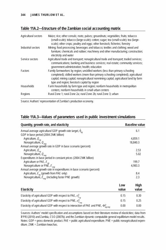
344 JAMES THURLOW ET AL.
Table 11A.2—Structure of the Zambian social accounting matrix
Agricultural sectors Maize; rice; other cereals; roots; pulses; groundnuts; vegetables; fruits; tobacco (small-scale); tobacco (large-scale); cotton; sugar; tea (small-scale); tea (large-
scale); other crops; poultry and eggs; other livestock; fisheries; forestryIndustrial sectors Mining; food processing; beverages and tobacco; textiles and clothing; wood and furniture; chemicals and rubber; machinery and other manufacturing; construction;
electricity and waterService sectors Agricultural trade and transport; nonagricultural trade and transport; traded services; communications; banking and business services; real estate; community services;
government administration; health; educationFactors Family farmworkers by region; unskilled workers (less than primary schooling completed); skilled workers (more than primary schooling completed); agricultural
capital; mining capital; nonagricultural nonmining capital; agricultural land by farm type and region; livestock capital by region
Households Farm households by farm type and region; nonfarm households in metropolitan centers; nonfarm households in small urban centers Regions Rural Zone 1; rural Zone 2a; rural Zone 2b; rural Zone 3; urban
Source: Authors’ representation of Zambia’s production economy.
Table 11A.3—Values of parameters used in public investment simulations
Quantity, growth rate, and elasticity Baseline valueAnnual average agricultural GDP growth rate target, θag 6.1GDP in base period (2004 ZMK billion) Agriculture, Qag 4,859.1 Nonagriculture, Qnag 18,840.3Annual average growth rate in GDP in base scenario (percent) Agriculture, Qag 2.53 Nonagriculture, Qnag 5.02Expenditures in base period in constant prices (2004 ZMK billion) Agriculture or PAE, Eag 199.7 Nonagriculture or PNE, Enag 4,983.3Annual average growth rate in expenditures in base scenario (percent) Agriculture, Eag
(growth from PAE only) 8.4 Nonagriculture, Enag
(including faster PNE growth) 2.3
Low HighElasticity value valueElasticity of agricultural GDP with respect to PAE, εQ
Eag 0.15 0.30
Elasticity of agricultural GDP with respect to PNE, εQEnag
0.15 0.25Elasticity of agricultural GDP with respect to interaction of PAE and PNE, ΦQ
ag,nag 0.00 0.00
Sources: Authors’ model specification and assumptions based on their literature review of elasticities; data from IFPRI (2010) and Zambia, CSO (2007b); and the Zambian dynamic computable general equilibrium model results.Notes: GDP = gross domestic product. PAE = public agricultural expenditure. PNE = public nonagricultural expen-diture. ZMK = Zambian kwachas.
ZAMBIA 345
ReferencesBarnett, T., J. Tumushabe, G. Bantebya, R. Ssebuliba, J. Ngasongwa, D. Kapinga, M. Ndelike,
M. Drinkwater, G. Mitti, and M. Haslwimmer. 1995. “The Social and Economic Impact of HIV/
AIDS on Farming Systems and Livelihoods in Rural Africa: Some Experience and Lessons from
Uganda, Tanzania and Zambia.” Journal of International Development 7 (1): 163–176.
Bezuneha, M., G. C. W. Amesb, and C. C. Mabbs-Zenoc. 1995. “Sustainable Agricultural Development
Using a Farming Systems Approach in Zambia.” Ecological Economics 15 (2): 149–156.
Breisinger, C., and J. Thurlow. 2008. Asian-Driven Resource Booms in Africa: Rethinking the Impacts on
Development. Discussion Paper 747. Washington, DC: International Food Policy Research
Institute.
Coulter, J., and G. Onumah. 2002. “The Role of Warehouse Receipt Systems in Enhanced Commodity
Marketing and Rural Livelihoods in Africa.” Food Policy 27 (4): 319–337.
Elliot, H., and P. T. Perrault. 2006. “Zambia: A Quiet Crisis in African Research and Development.” In
Agricultural R&D in the Developing World: Too Little, Too Late?, edited by P. G. Pardey, J. M. Altson,
and R. R. Piggot, 227–256. Washington, DC: International Food Policy Research Institute.
Fan, S., ed. 2008. Public Expenditures, Growth, and Poverty: Lessons from Developing Countries. Baltimore:
Johns Hopkins University Press.
Fan, S., and X. Zhang. 2008. “Public Expenditure, Growth, and Poverty Reduction in Rural Uganda.
Development.” African Development Review 20 (3): 466–496.
FAO (Food and Agriculture Organization of the United Nations). 2007. FAOSTAT Statistical Database.
Accessed September 16, 2011. http://faostat.fao.org/.
Govereh, J., J. J. Shawa, E. Malawo, and T. S. Jayne. 2006. Raising the Productivity of Public Investments
in Zambia’s Agricultural Sector. Working Paper 20. Lusaka, Zambia: Food Security Research
Project.
Hazell, P. B. R., and B. Hojjati. 1995. “Farm/Non-Farm Growth Linkages in Zambia.” Journal of
African Economies 4 (3): 406-435.
IFPRI (International Food Policy Research Institute). 2007. Agricultural Science and Technology
Indicators. Washington, DC. Accessed December 15. www.asti.cgiar.org/.
———. 2010. Statistics on Public Expenditure for Economic Development (SPEED) Database.
Accessed January 12. www.ifpri.org/book-39/ourwork/programs/priorities-public-investment/
speed-database.
IRF (International Road Federation). 2007. World Road Statistics. Geneva.
Jayne, T. S., J. Govereh, M. Wanzala, and M. Demeke. 2003. “Fertilizer Market Development: A
Comparative Analysis of Ethiopia, Kenya, and Zambia.” Food Policy 28 (4): 293–316.
Jayne, T. S., J. Govereh, P. Chilonda, N. Mason, A. Chapoto, and H. Haantuba. 2007. Trends in
Agricultural and Rural Development Indicators in Zambia. Working Paper 24. Lusaka, Zambia:
Food Security Research Project.
346 JAMES THURLOW ET AL.
McCulloch, N., B. Baulch, and M. Cherel-Robson. 2001. Poverty, Inequality and Growth in Zambia
during the 1990s. Discussion Paper 2001-123. Helsinki, Finland: World Institute for Development
Economic Research.
Nin Pratt, A., and B. Yu. 2008. An Updated Look at the Recovery of Agricultural Productivity in Sub-
Saharan Africa. Discussion Paper 787. Washington, DC: International Food Policy Research
Institute.
Phiri, D., S. Franzel, P. Mafongoya, I. Jered, R. Katanga, and S. Phiri. 2004. “Who Is Using the New
Technology? The Association of Wealth Status and Gender with the Planting of Improved Tree
Fallows in Eastern Province, Zambia.” Agricultural Systems 79 (2): 131–144.
Rosegrant, M. W., and R. E. Evenson. 1995. Total Factor Productivity and Sources of Long-Term Growth
in Indian Agriculture. Environment and Production Technology Discussion Paper 7. Washington,
DC: International Food Policy Research Institute.
Seshamani, V. 1999. “The Impact of Market Liberalization on Food Security in Zambia.” Food Policy
23 (6): 539–551.
Spencer, D. 1994. Infrastructure and Technology Constraints to Agricultural Development in the Humid
and Subhumid Tropics of Africa. Environment and Production Technology Division Discussion
Paper 3. Washington, DC: International Food Policy Research Institute.
Thirtle, C., L. Lin, and J. Piesse. 2003. “The Impact of Research-Led Agricultural Productivity Growth
on Poverty Reduction in Africa, Asia and Latin America.” World Development 31 (12):
1959–1975.
Thurlow, J., and P. Wobst. 2006. “Not All Growth Is Equally Good for the Poor: The Case of Zambia.”
Journal of African Economies 15 (4): 603–625.
Thurlow, J., S. Robinson, and D. Evans. 2005. Zambia: Social Accounting Matrix, 2001. Washington,
DC: International Food Policy Research Institute.
Thurlow, J., T. Zhu, and X. Diao. 2009. The Impact of Climate Variability and Change on Economic
Growth and Poverty in Zambia. Discussion Paper 890. Washington, DC: International Food Policy
Research Institute.
Wiegers, E., J. Curry, A. Garbero, and J. Hourihan. 2006. “Patterns of Vulnerability to AIDS Impacts
in Zambian Households.” Development and Change 37 (5): 1073–1092.
World Bank. 2010. World Development Indicators. Washington, DC.
Zambia, CSO (Central Statistical Offi ce). 2005. 2004 Living Conditions Monitoring Survey. Lusaka,
Zambia.
———. 2007a. Bulletin of Statistics (December 2007). Lusaka, Zambia.
———. 2007b. Government Financial Statistics. Lusaka, Zambia.
———. 2010. Living Conditions: Poverty in Zambia 1991–2001. Lusaka, Zambia. Accessed April 3,
2012. www.zamstats.gov.zm/lcm.php.
ZAMBIA 347
Zambia, MACO (Ministry of Agriculture and Cooperatives). 2007a. District Agricultural Production
Data Series. Lusaka, Zambia.
———. 2007b. Crop Production Guidelines. Lusaka, Zambia: Zambia Agriculture Research Institute,
Ministry of Agriculture and Cooperatives.
Zambia, MFNP (Ministry of Finance and National Planning). 2006. Fifth National Development Plan:
Broad Based Wealth and Job Creation through Citizenry Participation and Technological Advance-
ment. Lusaka, Zambia.
Zambia, NFRA (National Road Fund Agency). 2009. ROADSIP. Accessed April 3, 2012. www.nrfa
.org.zm/index.php?option=com_content&view=article&id=55&Itemid=11.
Zulu, B., J. J. Nijhoff, T. S. Jayne, and A. Negassa. 2000. Is the Glass Half Empty or Half Full? An Analysis
of Agricultural Production Trends in Zambia. Working Paper 3. Lusaka, Zambia: Food Security
Research Project.


C h a p t e r 1 2
MozambiqueJames Thurlow
A fter emerging from civil war in 1994 as one of the world’s poorest countries, Mozambique has since become one the world’s fastest growing countries. Gross domestic product (GDP) grew at 8 percent per year during 1996–
2003 while the national poverty rate fell from 69 to 55 percent (World Bank 2010). Much of this poverty reduction occurred in rural areas, where a rebound in agricul-tural production led to large improvements in household incomes and food security. However, even though the economy has continued to grow at more than 7 percent during 2003–09, the benefits to the poor have diminished. The national poverty rate remained virtually unchanged during this period (Mozambique, MPD 2010), mainly because of the poor performance of the agricultural sector and the effects of the 2008 food price crisis on urban households (see Arndt et al. 2008, 2010).
Agriculture’s poor performance is not due to low agroecological potential—in fact, Mozambique is land abundant and has some of the most favorable conditions for agriculture in Sub-Saharan Africa (Diao et al. 2007). Nor is it due to a lack of investments in education and health, as indicators for both these outcomes have continued to improve after 2003 (World Bank 2010). Rather, agriculture’s poor performance is mainly due to (1) an immense development defi cit caused by civil war (see, for example, Kyle 1991; Tschirley and Weber 1994); (2) a growth strategy focused on heavy industry “megaprojects”; and (3) generally weak public sector engagement in the agricultural sector. The third explanation above is refl ected in the constraints facing smallholder farmers in Mozambique—many of which could be addressed through common policy interventions. These constraints include, among others, the absence of an effective national research and extension system; in-adequate infrastructure, particularly rural roads (Arndt et al. 2000; Tarp et al. 2002);
350 JAMES THURLOW
and low provision and adoption of modern inputs, such as fertilizer and improved seeds (Tschirley and Benica 2001; Heltberg and Tarp 2002; Uaiene 2008). As a result, Mozambique has some of the lowest crop yields in Africa (FAO 2008). Although there have been some successes in growing export crops through out-grower schemes (Strasberg 1997; Benfi ca 2006), these initiatives remain small and localized and so have not had discernable impacts at the national level. Clearly there is need for a more comprehensive and concerted strategy in Mozambique to raise agricultural productivity and support broadly based rural development.
Both the weakness and importance of agriculture have been recognized by the Government of Mozambique. This acknowledgment is perhaps most evident in the country’s recent commitment to the Comprehensive Africa Agriculture Development Programme (CAADP), which was launched by the 2003 Maputo Declaration of the African Union. A key objective in this program is for African countries to reach and sustain at least 6 percent annual agricultural growth while also allocating at least 10 percent of their public resources to the agricultural sector. It is hoped that by increasing the level and effi ciency of agricultural investments, Mozambique will be able to increase foodcrop production, reduce rural poverty, and enhance food secu-rity at both the national and local levels.
Beyond the government’s renewed commitment to agriculture, there is also considerable foreign interest to grow new export crops in Mozambique. Most prominent among these are biofuels. By 2009, the government had received requests from foreign companies for land-use rights covering more than 12 mil-lion hectares to be used for feedstock cultivation (Arndt et al. 2010). This is more than double the amount of land currently cultivated for nonbiofuel crops in Mozambique. Although not all the requests were considered credible, proposals of more than half a million hectares had been approved by the end of 2009 for biofuels production (mainly to grow sugarcane and jatropha). Studies suggest that these biofuel investments will bolster economic growth and poverty reduction (see, for example, Arndt et al. 2010). What is not considered by these studies is whether promoting biofuels is preferable to investing in existing crops, particu-larly food staples. Addressing this concern would help prioritize government engagement in the agricultural sector, particularly in deciding between export- and staples-led growth strategies.
Mozambique’s high agricultural potential and land abundance mean that it has the option of not only expanding its production of food and nontraditional export crops but also exploring new growth opportunities, like biofuels. In this chapter I evaluate different agricultural growth paths for Mozambique in terms of their ability to generate economywide economic growth and reduce poverty throughout the country. For this, I develop a recursive dynamic computable general
MOZAMBIQUE 351
equilibrium (DCGE) model based on the one described in Chapter 2 of this volume. One of the distinctive features of this case study is the extension of the DCGE model to include new biofuels sectors, which allows for an assessment of how these new crops may (or may not) be preferable to existing food and export crops. This potential for entirely new technologies is unique to the Mozambique case study.
The chapter is structured as follows. I fi rst briefl y review the structure of Mozambique’s agricultural sector. The structure of the Mozambican DCGE model and its underlying data sources are described next. The model results are then pre-sented for the baseline growth scenario and the accelerated agricultural growth scenarios. The chapter concludes by summarizing the fi ndings and their implica-tions for designing a new agricultural development strategy in Mozambique.
Agriculture in Mozambique
Agriculture’s Economic StructureAgriculture is a key sector in the Mozambican economy. In 2003 it generated more than one-quarter of total GDP, one-fi fth of export earnings, and four-fi fths of employment. Crop agriculture can be divided into two parts. On the one hand, there are smallholders who make up a majority of the country’s farmers and who rely heavily on low-technology inputs to produce foodcrops, mainly for subsistence. On the other hand, the country’s few large commercial farmers grow mainly tradi-tional export crops, such as sugarcane and tobacco. These plantations typically make greater use of modern inputs and capital, such as fertilizer and irrigation. In between these two groups are a number of outgrower schemes, which engage smallholders in vertical supply chains growing export crops like cotton. These schemes often provide farmers with improved inputs in return for them agreeing to sell their har-vests at agreed-upon prices.
Mozambique has a mixed farming system dominated by maize and cassava, which together generated two-fi fths of agricultural GDP in 2003. Other cereals are also key staples, although their production is concentrated in certain subnational regions. For example, rice is mainly grown in the two central provinces of Zambezia and Sofala, whereas sorghum and millet are grown more intensively in the northern provinces (see Table 12A.1 in the appendix to this chapter). Traditional export crops are even more concentrated. For example, tea is grown in Manica, tobacco in Niassa and Tete, and sugarcane in the southernmost province surrounding Maputo (the capital city). Many of these food and export crops have links to downstream sectors, such as grain milling and the local refi ning of sugarcane. Together these agro- and
352 JAMES THURLOW
food-processing activities accounted for an additional 6 percent of total GDP and 5 percent of exports. The key characteristics of Mozambique’s 10 rural provinces and its urban centers are presented in Table 12.1.
The most important noncrop subsector in agriculture is ocean fi sheries. Although it generates only 2 percent of total GDP, it accounts for almost 20 percent of national export earnings. This is the second most important export sector after aluminum. In contrast, livestock is a relatively small sector in Mozambique—less than 2 percent of total GDP with virtually no exports. The livestock sector does, however, have strong downstream linkages. Although the fi sheries subsector mainly exports fresh or unprocessed seafood, livestock has stronger linkages to the meat sector in manufacturing.
Biofuel Production TechnologiesTwo biofuel feedstock crops have received considerable attention in Mozambique, namely, jatropha for producing biodiesel and sugarcane for ethanol (Arndt et al. 2010). The proposals received by the government from foreign companies inter-ested in producing biofuels in Mozambique differ in terms of their production arrangements. Most requests for land for sugarcane envisage using a plantation approach to producing the feedstock. In contrast, proposals involving jatropha typi-cally adopt outgrower approaches. Therefore, as production of these two crops expands over the coming decade, they will have very different implications for smallholder farmers. Given Mozambique’s abundance of favorable land, it is reason-able to expect that all the biofuel feedstock could be produced on currently un-cultivated lands. However, although land may not be as great a constraint in Mozambique as in other African countries, there are defi nite labor shortages in the rural economy, especially during key planting and harvesting periods. Thus, grow-ing biofuel feedstock will have implications for other crops, as it requires that labor be reallocated away from existing farm and nonfarm activities.
The analysis assigns specifi c technologies to jatropha- and sugarcane-based biofuel production, which are drawn from a microlevel study conducted by Econergy (2008). Broadly speaking, jatropha is more low-skilled labor-intensive than sugar-cane, because the former is produced using smallholder farmers (see Arndt et al. 2010). Jatropha is also a more land-intensive crop per liter of biofuel produced, because of the biophysical and energy characteristics of this crop. Finally, plantation-based sugarcane is more capital intensive than jatropha. Based on current proposals, all the capital required to establish new biofuels industries in Mozambique will come from abroad (through foreign direct investment). It is also anticipated that most profi ts will be repatriated to the foreign companies. Given the uncertainty over future biofuels production in Mozambique, the analysis assumes that biofuels pro-
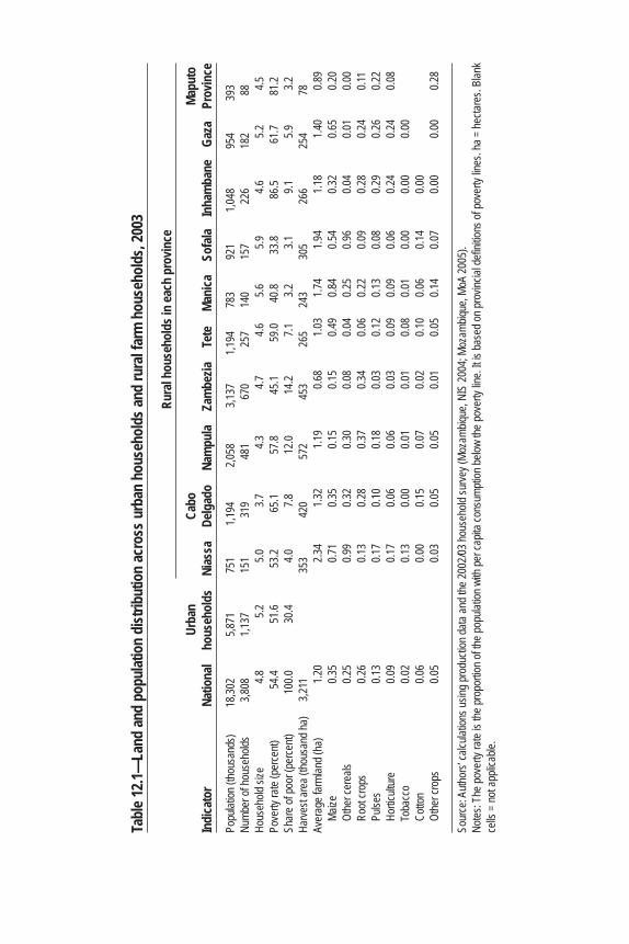
Tabl
e 12.1
—La
nd an
d po
pulat
ion
dist
ribut
ion
acro
ss u
rban
hou
seho
lds a
nd ru
ral f
arm
hou
seho
lds,
2003
Ru
ral h
ouse
hold
s in
each
pro
vince
Urba
n
Cabo
Mapu
toIn
dica
tor
Natio
nal
hous
ehol
ds
Nias
sa
Delg
ado
Nam
pula
Zam
bezia
Te
te
Mani
ca
Sofa
la In
ham
bane
Ga
za
Prov
ince
Popu
lation
(tho
usan
ds)
18,30
2 5,8
71
751
1,194
2,0
58
3,137
1,1
94
783
921
1,048
95
4 39
3Nu
mber
of ho
useh
olds
3,808
1,1
37
151
319
481
670
257
140
157
226
182
88Ho
useh
old si
ze
4.8
5.2
5.0
3.7
4.3
4.7
4.6
5.6
5.9
4.6
5.2
4.5Po
verty
rate
(per
cent)
54
.4 51
.6 53
.2 65
.1 57
.8 45
.1 59
.0 40
.8 33
.8 86
.5 61
.7 81
.2Sh
are o
f poo
r (pe
rcent)
10
0.0
30.4
4.0
7.8
12.0
14.2
7.1
3.2
3.1
9.1
5.9
3.2Ha
rvest
area
(tho
usan
d ha)
3,2
11
35
3 42
0 57
2 45
3 26
5 24
3 30
5 26
6 25
4 78
Aver
age f
arml
and (
ha)
1.20
2.3
4 1.3
2 1.1
9 0.6
8 1.0
3 1.7
4 1.9
4 1.1
8 1.4
0 0.8
9
Maize
0.3
5
0.71
0.35
0.15
0.15
0.49
0.84
0.54
0.32
0.65
0.20
Ot
her c
erea
ls 0.2
5
0.99
0.32
0.30
0.08
0.04
0.25
0.96
0.04
0.01
0.00
Ro
ot cro
ps
0.26
0.1
3 0.2
8 0.3
7 0.3
4 0.0
6 0.2
2 0.0
9 0.2
8 0.2
4 0.1
1
Pulse
s 0.1
3
0.17
0.10
0.18
0.03
0.12
0.13
0.08
0.29
0.26
0.22
Ho
rticult
ure
0.09
0.1
7 0.0
6 0.0
6 0.0
3 0.0
9 0.0
9 0.0
6 0.2
4 0.2
4 0.0
8
Toba
cco
0.02
0.1
3 0.0
0 0.0
1 0.0
1 0.0
8 0.0
1 0.0
0 0.0
0 0.0
0
Cotto
n 0.0
6
0.00
0.15
0.07
0.02
0.10
0.06
0.14
0.00
Othe
r cro
ps
0.05
0.0
3 0.0
5 0.0
5 0.0
1 0.0
5 0.1
4 0.0
7 0.0
0 0.0
0 0.2
8
Sour
ce: A
uthor
s’ ca
lculat
ions u
sing p
rodu
ction
data
and t
he 20
02/03
hous
ehold
surve
y (Mo
zamb
ique,
NIS
2004
; Moz
ambiq
ue, M
oA 20
05).
Notes
: The
pove
rty ra
te is
the pr
opor
tion o
f the p
opula
tion w
ith pe
r cap
ita co
nsum
ption
below
the p
over
ty lin
e. It i
s bas
ed on
prov
incial
defin
itions
of po
verty
lines
. ha =
hecta
res.
Blan
k ce
lls =
not a
pplic
able.
354 JAMES THURLOW
duction will be evenly balanced across sugarcane and jatropha feedstock (that is, both small- and large-scale production approaches).
The Mozambican DCGE ModelA new DCGE model was developed for Mozambique to capture the relationship between economic growth and household incomes and poverty. The model is cali-brated to a regionalized version of the 2003 social accounting matrix (SAM) docu-mented in McCool, Thurlow, and Arndt (2009). The SAM’s economywide structure allows the model to measure the effects of economic linkages between agricultural and nonagricultural sectors. The detailed structure of the model separates producers into 56 sectors, 24 of which are in agriculture (see Table 12A.2 in the appendix to this chapter). To design the subsector growth scenarios, agricultural crops are sepa-rated into fi ve broad groups: (1) cereal crops (for example, maize, rice, sorghum, and millet), (2) roots (cassava and potatoes), (3) pulses and nuts (for example, beans and groundnuts), (4) horticulture, and (5) high-value export crops (such as tobacco and cotton). The model also includes two new biofuel feedstock subsectors: jatropha for biodiesel production and sugarcane for ethanol production. To com-plete the agricultural sector, the model includes livestock, forestry, and fi sheries subsectors. Sectoral production and commodity demand in the SAM are from offi cial national accounts and supply–use tables for 2003 (Mozambique, NIS 2007). Crop-production technologies were drawn from a 1996 input–output table (Arndt et al. 1998), with the exception of the biofuels crops, whose technologies were described in the previous section.
The model also captures heterogeneity in subnational production patterns. Rural agricultural production is disaggregated across Mozambique’s 10 provinces, refl ecting varying agroecological conditions in the country. Province-level agricul-tural production and area data were taken from the 2005 national agricultural survey (Mozambique, MoA 2005). Where information on certain crops, such as horticulture, was missing from the survey, data were taken from FAO (2008). To capture the distinct characteristics of the urban economy, urban areas in each prov-ince are grouped into a single region, although agriculture remained within rural regions because of a lack of production data for urban agriculturalists. Finally, Maputo City is treated as a separate metropolitan region. Thus, there are a total of 12 subnational regions in the model. Certain factor markets are segmented across regions, including those of agricultural land and family farmworkers. These factors can migrate between farm activities but not between regions. In contrast, unskilled, semiskilled, and skilled labor can migrate across both sectors and regions. Finally, capital is sector-specifi c and once invested cannot be transferred to new activities.
MOZAMBIQUE 355
New capital is generated from past investment and is allocated to sectors based on their relative profi tability.
The model is calibrated to the initial cropping patterns for 2005 in the rural areas of each of the 10 provinces. The representative farmer in each province responds to changes in production technology and commodity demand and prices by reallocating land across different crops to maximize income. These farmers also reallocate their labor and capital between farm and nonfarm activities, including livestock and fi shing, wage employment, and diversifi cation into nonagricultural sectors, such as transport, trade, and construction. Thus, by capturing production information across subnational regions, the DCGE model combines the national or macroeconomic consistency of an economywide model with the detail of a province-level agricultural sector or representative farm model. The DCGE model is thus an ideal tool for measuring the unique growth linkages and income and price effects resulting from accelerating growth in specifi c agricultural subsectors.
Finally, the model determines the effect of growth on households’ incomes and consumption. There are 66 representative household groups in the model, dis-aggregated by nationally defi ned per capita expenditure quintiles and 12 regions, with the top quintile in urban centers and metropolitan Maputo further disaggre-gated into four income groups. Each household in the 2002/03 national household survey (Mozambique, NIS 2004) is linked to its corresponding representative household in the model. Changes in representative households’ consumption and prices in the DCGE model are passed down to corresponding households in the survey, where total consumption expenditures are recalculated. This new level of per capita expenditure is compared to the offi cial poverty line to determine whether the household’s poverty status has changed. Estimated changes in poverty from the DCGE model therefore capture differences in households’ consumption patterns and income distribution as refl ected in the survey. The new DCGE model for Mozambique can therefore translate changes in production levels to changes in both factor and products prices, and it calculates how these modify household incomes and consumption patterns, thus determining poverty rates in different regions and population groups.
Baseline Growth ScenarioThe DCGE model is fi rst used to examine the impact of Mozambique’s current growth path on poverty reduction. This baseline scenario draws on historical pro-duction trends for individual agricultural and nonagricultural subsectors. Mozambique experienced rapid growth during 1996–2003, with national GDP growing at almost 9 percent per year (Mozambique, NIS 2007). During this time
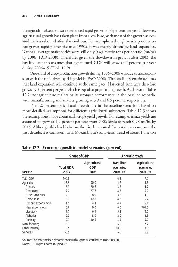
356 JAMES THURLOW
the agricultural sector also experienced rapid growth of 6 percent per year. However, agricultural growth has taken place from a low base, with most of the growth associ-ated with a rebound after the civil war. For example, although maize production has grown rapidly after the mid-1990s, it was mostly driven by land expansion. National average maize yields were still only 0.83 metric tons per hectare (mt/ha) by 2006 (FAO 2008). Therefore, given the slowdown in growth after 2003, the baseline scenario assumes that agricultural GDP will grow at 4 percent per year during 2006–15 (Table 12.2).
One-third of crop-production growth during 1996–2006 was due to area expan-sion with the rest driven by rising yields (FAO 2008). The baseline scenario assumes that land expansion will continue at the same pace. Harvested land area therefore grows by 2 percent per year, which is equal to population growth. As shown in Table 12.2, nonagriculture maintains its stronger performance in the baseline scenario, with manufacturing and services growing at 5.9 and 6.5 percent, respectively.
The 4.2 percent agricultural growth rate in the baseline scenario is based on more detailed assumptions for different agricultural subsectors. Table 12.3 shows the assumptions made about each crop’s yield growth. For example, maize yields are assumed to grow at 1.9 percent per year from 2006 levels to reach 0.98 mt/ha by 2015. Although this level is below the yields reported for certain seasons over the past decade, it is consistent with Mozambique’s long-term trend of about 1 one ton
Table 12.2—Economic growth in model scenarios (percent)
Share of GDP Annual growth
Agricultural Baseline Agriculture Total GDP, GDP, scenario, scenario, Sector 2003 2003 2006–15 2006–15Total GDP 100.0 6.3 7.0Agriculture 25.9 100.0 4.2 6.6 Cereals 5.3 20.6 3.5 4.7 Root crops 7.2 27.7 4.7 5.2 Pulses and nuts 2.3 8.9 3.6 4.3 Horticulture 3.3 12.8 4.3 5.7 Existing export crops 1.1 4.1 4.7 6.1 New export crops 0.0 0.0 0.0 765.0 Livestock 1.7 6.4 5.2 6.0 Fisheries 2.3 8.9 2.0 3.6 Forestry 2.7 10.6 5.3 6.0Manufacturing 13.7 5.9 7.2Other industry 9.5 10.0 8.5Services 50.9 6.5 6.9
Source: The Mozambican dynamic computable general equilibrium model results. Note: GDP = gross domestic product.
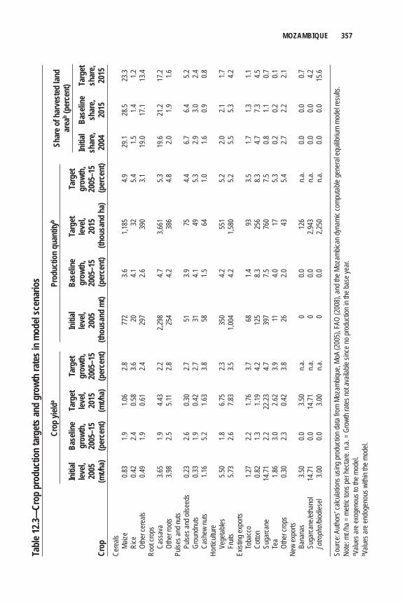
MOZAMBIQUE 357Ta
ble 1
2.3—
Crop
pro
duct
ion
targ
ets a
nd g
rowt
h ra
tes i
n m
odel
scen
ario
s
Cr
op yi
elda
Prod
uctio
n qu
antit
yb
In
itial
Base
line
Targ
et
Targ
et
Initi
al Ba
selin
e Ta
rget
Ta
rget
level,
gr
owth
, lev
el,
grow
th,
level,
gr
owth
, lev
el,
grow
th,
Initi
al Ba
selin
e Ta
rget
20
05
2005
–15
2015
20
05–1
5 20
05
2005
–15
2015
20
05–1
5 sh
are,
shar
e, sh
are,
Crop
(m
t/ha)
(p
erce
nt)
(mt/h
a)
(per
cent
) (t
hous
and
mt)
(per
cent
) (t
hous
and
ha)
(per
cent
) 20
04
2015
20
15Ce
reals
Maize
0.8
3 1.9
1.0
6 2.8
77
2 3.6
1,1
85
4.9
29.1
28.5
23.3
Ri
ce
0.42
2.4
0.58
3.6
20
4.1
32
5.4
1.5
1.4
1.2
Othe
r cer
eals
0.4
9 1.9
0.6
1 2.4
29
7 2.6
39
0 3.1
19
.0 17
.1 13
.4Ro
ot cro
ps
Ca
ssav
a 3.6
5 1.9
4.4
3 2.2
2,2
98
4.7
3,661
5.3
19
.6 21
.2 17
.2
Othe
r roo
ts 3.9
8 2.5
5.1
1 2.8
25
4 4.2
38
6 4.8
2.0
1.9
1.6
Pulse
s and
nuts
Pu
lses a
nd oi
lseed
s 0.2
3 2.6
0.3
0 2.7
51
3.9
75
4.4
6.7
6.4
5.2
Gr
ound
nuts
0.33
1.9
0.42
2.7
31
4.1
49
5.3
2.9
3.0
2.4
Cash
ew nu
ts 1.1
6 5.2
1.6
3 3.8
58
1.5
64
1.0
1.6
0.9
0.8
Hortic
ultur
e
Vege
tables
5.5
0 1.8
6.7
5 2.3
35
0 4.2
55
1 5.2
2.0
2.1
1.7
Fr
uits
5.73
2.6
7.83
3.5
1,004
4.2
1,5
80
5.2
5.5
5.3
4.2Ex
isting
expo
rts
To
bacc
o 1.2
7 2.2
1.7
6 3.7
68
1.4
93
3.5
1.7
1.3
1.1
Co
tton
0.82
1.3
1.19
4.2
125
8.3
256
8.3
4.7
7.3
4.5
Suga
rcane
14
.71
2.2
22.23
4.7
39
7 7.5
76
0 7.5
0.8
1.1
0.7
Te
a 1.8
6 3.0
2.6
2 3.9
11
4.0
17
5.3
0.2
0.2
0.1
Ot
her c
rops
0.3
0 2.3
0.4
2 3.8
26
2.0
43
5.4
2.7
2.2
2.1
New
expo
rts
Ba
nana
s 3.5
0 0.0
3.5
0 n.a
. 0
0.0
126
n.a.
0.0
0.0
0.7
Suga
rcane
/ etha
nol
14.71
0.0
14
.71
n.a.
0 0.0
2,9
43
n.a.
0.0
0.0
4.2
Jatro
pha /
biodie
sel
3.00
0.0
3.00
n.a.
0 0.0
2,2
50
n.a.
0.0
0.0
15.6
Sour
ce: A
uthor
s’ ca
lculat
ions u
sing p
rodu
ction
data
from
Moza
mbiqu
e, Mo
A (2
005)
, FAO
(200
8), a
nd th
e Moz
ambic
an dy
nami
c com
putab
le ge
nera
l equ
ilibriu
m mo
del re
sults
.No
te: m
t / ha
= m
etric
tons p
er he
ctare
. n.a.
= G
rowt
h rate
s not
avail
able
since
no pr
oduc
tion i
n the
base
year.
a Value
s are
exog
enou
s to t
he m
odel.
b Value
s are
endo
geno
us w
ithin
the m
odel.
Shar
e of h
arve
sted
land
ar
eab (p
erce
nt)
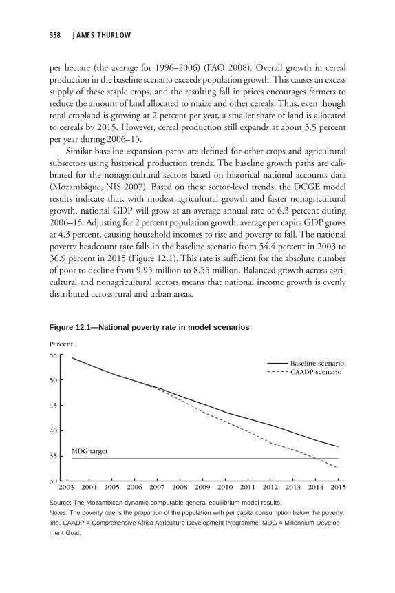
358 JAMES THURLOW
per hectare (the average for 1996–2006) (FAO 2008). Overall growth in cereal production in the baseline scenario exceeds population growth. This causes an excess supply of these staple crops, and the resulting fall in prices encourages farmers to reduce the amount of land allocated to maize and other cereals. Thus, even though total cropland is growing at 2 percent per year, a smaller share of land is allocated to cereals by 2015. However, cereal production still expands at about 3.5 percent per year during 2006–15.
Similar baseline expansion paths are defi ned for other crops and agricultural subsectors using historical production trends. The baseline growth paths are cali-brated for the nonagricultural sectors based on historical national accounts data (Mozambique, NIS 2007). Based on these sector-level trends, the DCGE model results indicate that, with modest agricultural growth and faster nonagricultural growth, national GDP will grow at an average annual rate of 6.3 percent during 2006–15. Adjusting for 2 percent population growth, average per capita GDP grows at 4.3 percent, causing household incomes to rise and poverty to fall. The national poverty headcount rate falls in the baseline scenario from 54.4 percent in 2003 to 36.9 percent in 2015 (Figure 12.1). This rate is suffi cient for the absolute number of poor to decline from 9.95 million to 8.55 million. Balanced growth across agri-cultural and nonagricultural sectors means that national income growth is evenly distributed across rural and urban areas.
Percent
55Baseline scenario
MDG target
30
50
45
40
35
2015201420132012201120102009200820072006200520042003
CAADP scenario
Figure 12.1—National poverty rate in model scenarios
Source: The Mozambican dynamic computable general equilibrium model results.Notes: The poverty rate is the proportion of the population with per capita consumption below the povertyline. CAADP = Comprehensive Africa Agriculture Development Programme. MDG = Millennium Develop-ment Goal.
MOZAMBIQUE 359
Accelerated Growth Scenarios
Impacts on Agricultural and National Economic GrowthThe baseline scenario refl ects a reasonable growth path for Mozambique based on published historical trends. This section examines the potential contribution of different agricultural subsectors in helping Mozambique achieve a 6 percent agri-cultural growth target—as identifi ed in the CAADP. To increase crop-production levels, the scenarios target faster yield growth rates (by raising total factor productiv-ity in individual subsectors). The targets are considered reasonable yield improve-ments based on discussions with the Department of Economics in the Ministry of Agriculture. Unlike the country studies reported in other chapters of this volume, the accelerated agricultural growth scenario is not based on the increased yields achieved under the ideal conditions of controlled fi eld trials.
Taking maize as an example, the baseline scenario assumes that average yields over the next 10 years would remain relatively constant at 0.83–0.98 mt/ha (see Table 12.3). The Agriculture scenario simulates more ambitious yield improve-ments. Maize yield’s growth rate rises from 1.9 percent in the baseline to 2.8 percent. Thus, average maize yields rise over the next 10 years to reach 1.1 mt/ha by 2015. This value is still below the potential yield identifi ed by Mozambique’s national agricultural research institute.
The Agriculture scenario similarly targets increased yields for other crops in each province. Particularly fast growth is targeted for existing export crops, because they are considered to have a higher growth potential than foodcrops. However, without information on region-specifi c growth potentials, the model assumes that yield increases are proportional across all regions, meaning that fi nal yields will vary according to initial yield estimates and the variation in local land and labor market conditions (for example, base-year cropping patterns and farm/nonfarm employ-ment opportunities). Production in the livestock, forestry, and fi sheries subsectors is not increased to achieve particular yield targets but rather to increase growth in real value-added. This decision was again based on a joint assessment with the Ministry of Agriculture. Combining the acceleration in growth in all agricultural subsectors produces the Agriculture growth scenario.
As discussed earlier in this chapter, Mozambique has the opportunity to sub-stantially expand domestic production of various new export crops, including bio-fuel feedstocks. There is also scope for downstream processing of biodiesel and ethanol. The Agriculture scenario models an expansion of land allocated to biofuels. Based on existing investment requests, land allocated to sugarcane for ethanol pro-duction is assumed to rise to 200,000 hectares by 2015, whereas jatropha for bio-diesel production grows to 500,000 hectares. Following Arndt et al. (2010), it is assumed that all biofuels are exported after having been processed. From a balance
360 JAMES THURLOW
of payments perspective, because Mozambique is a small economy and does not affect world prices, exporting all biofuels is equivalent to reducing traditional fuel imports (that is, there is no change in the current balance). Apart from biofuels, the scenario also allows for the production of new export-quality bananas produced on large-scale plantations. Land allocated to banana production is assumed to rise to 36,000 hectares in the Agriculture scenario. As with other crops, investment in each of these new crops is assumed to be evenly distributed across the 10 rural provinces.
Results from the DCGE model indicate that achieving the production targets identifi ed in Table 12.3 and allocating land to new export crops will allow Mozambique to reach the 6 percent annual agricultural growth target. More specifi -cally, average agricultural growth during 2006–15 would be 6.6 percent per year in the Agriculture scenario (see Table 12.2). Because agriculture makes up one-quarter of the economy, its acceleration also increases national GDP growth rate from 6.3 to 7.0 percent per year. Part of this additional national growth is due to economy-wide linkages. Faster agricultural growth stimulates additional nonagricultural growth by raising demand for farm inputs and lowering input prices for downstream processing sectors. For instance, the GDP growth rate of the manufacturing sector increases from 5.9 to 7.2 percent per year in the Agriculture scenario. Accelerating agricultural growth therefore has economywide implications.
Impacts on Household Incomes and Poverty Higher rates of economic growth cause the national poverty rate to fall farther than in the baseline scenario. This change is shown in Figure 12.1, where the share of the population under the poverty line is 32.6 percent by 2015 in the Agriculture sce-nario compared with 36.9 percent in the baseline. Because population growth remains constant between scenarios, an additional 0.98 million people are lifted above the poverty line by 2015 due to faster growth in the Agriculture scenario.
Although all representative household groups in the DCGE model benefi t from faster agricultural growth, not all benefi t equally. Table 12.4 reports changes in poverty rates for different population groups. Households in small provincial towns benefi t more from agricultural growth than do those in the large metropolitan centers. This is because these small towns engage more in agriculture-related activi-ties, such as food processing and local trade and transport. Agriculture’s downstream production linkages are thus stronger in small towns. Moreover, households in small towns typically spend a larger share of their incomes on agricultural goods, primarily foodcrops, than do residents in large cities. Consumption linkages with agriculture are therefore also stronger in small urban centers.
High-value export crops are grown more intensively in certain provinces. For example, tobacco production is most important in Niassa Province, whereas cotton
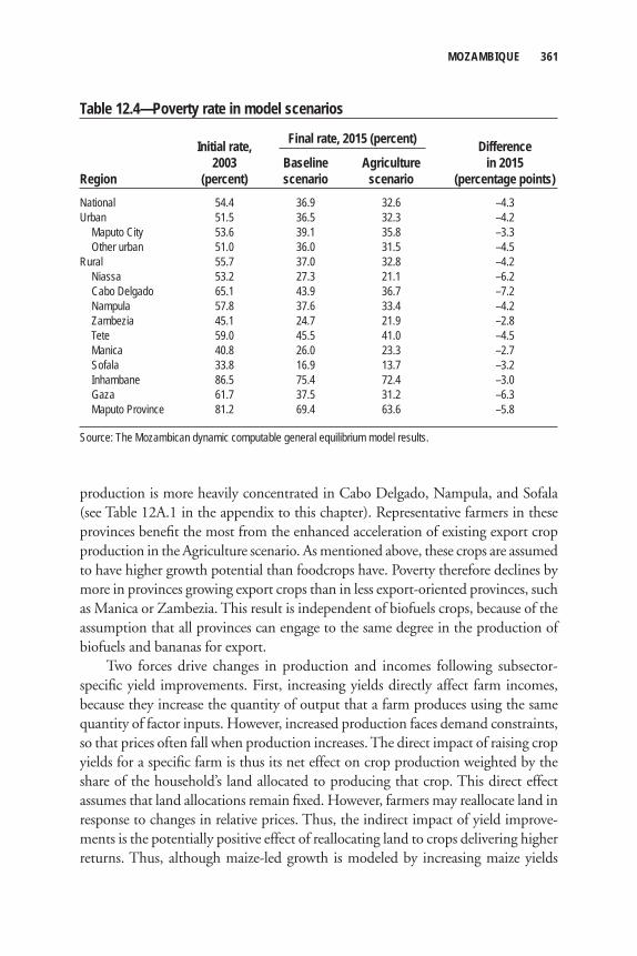
MOZAMBIQUE 361
production is more heavily concentrated in Cabo Delgado, Nampula, and Sofala (see Table 12A.1 in the appendix to this chapter). Representative farmers in these provinces benefi t the most from the enhanced acceleration of existing export crop production in the Agriculture scenario. As mentioned above, these crops are assumed to have higher growth potential than foodcrops have. Poverty therefore declines by more in provinces growing export crops than in less export-oriented provinces, such as Manica or Zambezia. This result is independent of biofuels crops, because of the assumption that all provinces can engage to the same degree in the production of biofuels and bananas for export.
Two forces drive changes in production and incomes following subsector-specifi c yield improvements. First, increasing yields directly affect farm incomes, because they increase the quantity of output that a farm produces using the same quantity of factor inputs. However, increased production faces demand constraints, so that prices often fall when production increases. The direct impact of raising crop yields for a specifi c farm is thus its net effect on crop production weighted by the share of the household’s land allocated to producing that crop. This direct effect assumes that land allocations remain fi xed. However, farmers may reallocate land in response to changes in relative prices. Thus, the indirect impact of yield improve-ments is the potentially positive effect of reallocating land to crops delivering higher returns. Thus, although maize-led growth is modeled by increasing maize yields
Table 12.4—Poverty rate in model scenarios
Initial rate, Difference 2003 Baseline Agriculture in 2015Region (percent) scenario scenario (percentage points)National 54.4 36.9 32.6 –4.3Urban 51.5 36.5 32.3 –4.2 Maputo City 53.6 39.1 35.8 –3.3 Other urban 51.0 36.0 31.5 –4.5Rural 55.7 37.0 32.8 –4.2 Niassa 53.2 27.3 21.1 –6.2 Cabo Delgado 65.1 43.9 36.7 –7.2 Nampula 57.8 37.6 33.4 –4.2 Zambezia 45.1 24.7 21.9 –2.8 Tete 59.0 45.5 41.0 –4.5 Manica 40.8 26.0 23.3 –2.7 Sofala 33.8 16.9 13.7 –3.2 Inhambane 86.5 75.4 72.4 –3.0 Gaza 61.7 37.5 31.2 –6.3 Maputo Province 81.2 69.4 63.6 –5.8
Source: The Mozambican dynamic computable general equilibrium model results.
Final rate, 2015 (percent)
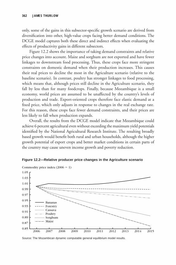
362 JAMES THURLOW
only, some of the gains in this subsector-specifi c growth scenario are derived from diversifi cation into other, high-value crops facing better demand conditions. The DCGE model captures both these direct and indirect effects when evaluating the effects of productivity gains in different subsectors.
Figure 12.2 shows the importance of taking demand constraints and relative price changes into account. Maize and sorghum are not exported and have fewer linkages to downstream food processing. Thus, these crops face more stringent constraints on domestic demand when their production increases. This causes their real prices to decline the most in the Agriculture scenario (relative to the baseline scenario). In contrast, poultry has stronger linkages to food processing, which means that, although prices still decline in the Agriculture scenario, they fall by less than for many foodcrops. Finally, because Mozambique is a small economy, world prices are assumed to be unaffected by the country’s levels of production and trade. Export-oriented crops therefore face elastic demand at a fi xed price, which only adjusts in response to changes in the real exchange rate. For this reason, these crops face fewer demand constraints, and their prices are less likely to fall when production expands.
Overall, the results from the DCGE model indicate that Mozambique could achieve 6 percent agricultural even without exceeding the maximum yield potentials identifi ed by the National Agricultural Research Institute. The resulting broadly based growth would benefi t both rural and urban households, although the higher growth potential of export crops and better market conditions in certain parts of the country may cause uneven income growth and poverty reduction.
Commodity price index (2006 � 1)
1.05
0.8520152014
PoultrySorghumMaize
CassavaForestryBananas
0.93
0.95
0.97
0.99
1.01
1.03
0.91
0.89
0.87
20132012201120102009200820072006
Figure 12.2—Relative producer price changes in the Agriculture scenario
Source: The Mozambican dynamic computable general equilibrium model results.
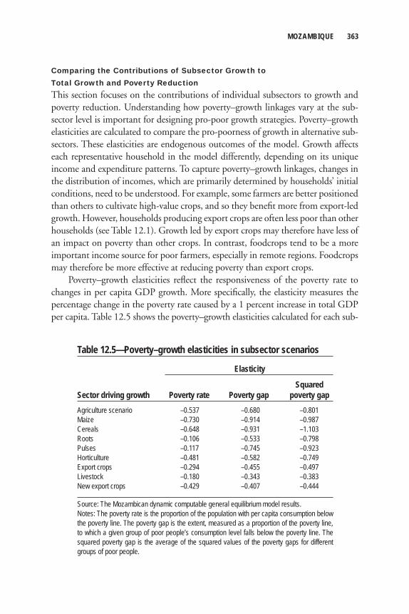
MOZAMBIQUE 363
Comparing the Contributions of Subsector Growth to Total Growth and Poverty ReductionThis section focuses on the contributions of individual subsectors to growth and poverty reduction. Understanding how poverty–growth linkages vary at the sub-sector level is important for designing pro-poor growth strategies. Poverty–growth elasticities are calculated to compare the pro-poorness of growth in alternative sub-sectors. These elasticities are endogenous outcomes of the model. Growth affects each representative household in the model differently, depending on its unique income and expenditure patterns. To capture poverty–growth linkages, changes in the distribution of incomes, which are primarily determined by households’ initial conditions, need to be understood. For example, some farmers are better positioned than others to cultivate high-value crops, and so they benefi t more from export-led growth. However, households producing export crops are often less poor than other households (see Table 12.1). Growth led by export crops may therefore have less of an impact on poverty than other crops. In contrast, foodcrops tend to be a more important income source for poor farmers, especially in remote regions. Foodcrops may therefore be more effective at reducing poverty than export crops.
Poverty–growth elasticities refl ect the responsiveness of the poverty rate to changes in per capita GDP growth. More specifi cally, the elasticity measures the percentage change in the poverty rate caused by a 1 percent increase in total GDP per capita. Table 12.5 shows the poverty–growth elasticities calculated for each sub-
Table 12.5—Poverty–growth elasticities in subsector scenarios
Elasticity
SquaredSector driving growth Poverty rate Poverty gap poverty gapAgriculture scenario –0.537 –0.680 –0.801Maize –0.730 –0.914 –0.987Cereals –0.648 –0.931 –1.103Roots –0.106 –0.533 –0.798Pulses –0.117 –0.745 –0.923Horticulture –0.481 –0.582 –0.749Export crops –0.294 –0.455 –0.497Livestock –0.180 –0.343 –0.383New export crops –0.429 –0.407 –0.444
Source: The Mozambican dynamic computable general equilibrium model results. Notes: The poverty rate is the proportion of the population with per capita consumption below the poverty line. The poverty gap is the extent, measured as a proportion of the poverty line, to which a given group of poor people’s consumption level falls below the poverty line. The squared poverty gap is the average of the squared values of the poverty gaps for different groups of poor people.
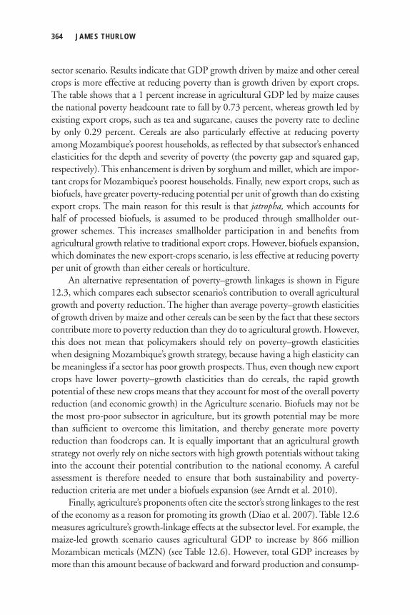
364 JAMES THURLOW
sector scenario. Results indicate that GDP growth driven by maize and other cereal crops is more effective at reducing poverty than is growth driven by export crops. The table shows that a 1 percent increase in agricultural GDP led by maize causes the national poverty headcount rate to fall by 0.73 percent, whereas growth led by existing export crops, such as tea and sugarcane, causes the poverty rate to decline by only 0.29 percent. Cereals are also particularly effective at reducing poverty among Mozambique’s poorest households, as refl ected by that subsector’s enhanced elasticities for the depth and severity of poverty (the poverty gap and squared gap, respectively). This enhancement is driven by sorghum and millet, which are impor-tant crops for Mozambique’s poorest households. Finally, new export crops, such as biofuels, have greater poverty-reducing potential per unit of growth than do existing export crops. The main reason for this result is that jatropha, which accounts for half of processed biofuels, is assumed to be produced through smallholder out-grower schemes. This increases smallholder participation in and benefi ts from agricultural growth relative to traditional export crops. However, biofuels expansion, which dominates the new export-crops scenario, is less effective at reducing poverty per unit of growth than either cereals or horticulture.
An alternative representation of poverty–growth linkages is shown in Figure 12.3, which compares each subsector scenario’s contribution to overall agricultural growth and poverty reduction. The higher than average poverty–growth elasticities of growth driven by maize and other cereals can be seen by the fact that these sectors contribute more to poverty reduction than they do to agricultural growth. However, this does not mean that policymakers should rely on poverty–growth elasticities when designing Mozambique’s growth strategy, because having a high elasticity can be meaningless if a sector has poor growth prospects. Thus, even though new export crops have lower poverty–growth elasticities than do cereals, the rapid growth potential of these new crops means that they account for most of the overall poverty reduction (and economic growth) in the Agriculture scenario. Biofuels may not be the most pro-poor subsector in agriculture, but its growth potential may be more than suffi cient to overcome this limitation, and thereby generate more poverty reduction than foodcrops can. It is equally important that an agricultural growth strategy not overly rely on niche sectors with high growth potentials without taking into the account their potential contribution to the national economy. A careful assessment is therefore needed to ensure that both sustainability and poverty-reduction criteria are met under a biofuels expansion (see Arndt et al. 2010).
Finally, agriculture’s proponents often cite the sector’s strong linkages to the rest of the economy as a reason for promoting its growth (Diao et al. 2007). Table 12.6 measures agriculture’s growth-linkage effects at the subsector level. For example, the maize-led growth scenario causes agricultural GDP to increase by 866 million Mozambican meticals (MZN) (see Table 12.6). However, total GDP increases by more than this amount because of backward and forward production and consump-
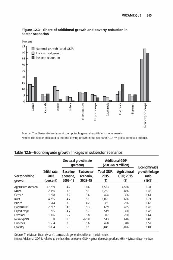
MOZAMBIQUE 365
Percent
45
0
25
20
35
40
30
15
10
5
Agricultural growth
National growth (total GDP)
Poverty reduction
Mai
ze
Cer
eals
Ho
rtic
ult
ure
Exp
ort
cro
ps
Live
sto
ck
Ro
ots
Pu
lses
Fore
stry
Fish
erie
s
New
ex
po
rt c
rop
s
Figure 12.3—Share of additional growth and poverty reduction in sector scenarios
Source: The Mozambican dynamic computable general equilibrium model results.Notes: The sector indicated is the one driving growth in the scenario. GDP = gross domestic product.
Table 12.6—Economywide growth linkages in subsector scenarios
Economywide Initial rate, Baseline Subsector Total GDP, Agricultural growth-linkageSector driving 2003 scenario, scenario, 2015 GDP, 2015 ratiogrowth (percent) 2005–15 2005–15 (1) (2) (1)/(2)Agriculture scenario 17,299 4.2 6.6 8,563 6,538 1.31Maize 2,356 3.6 5.1 1,227 866 1.42Cereals 1,208 3.2 3.6 494 306 1.61Root 4,795 4.7 5.1 1,091 636 1.71Pulses 1,544 3.6 4.2 381 236 1.62Horticulture 2,217 4.3 5.3 689 485 1.42Export crops 705 4.7 8.7 519 350 1.48Livestock 1,106 5.2 5.8 377 230 1.64New exports 0 0.0 765.0 513 616 0.83Fisheries 1,534 2.0 5.6 498 318 1.57Forestry 1,834 5.3 6.1 3,041 3,026 1.01
Source: The Mozambican dynamic computable general equilibrium model results.Notes: Additional GDP is relative to the baseline scenario. GDP = gross domestic product. MZN = Mozambican meticals.
Sectoral growth rate Additional GDP (percent) (2003 MZN million)
366 JAMES THURLOW
tion linkages. For example, increasing maize production stimulates growth in down-stream food processing while also reducing food prices and increasing real incomes that are then spent on nonagricultural commodities. Overall GDP increases by MZN1,227 million, which means that for every MZN1.00 increase in agricultural GDP driven by maize-led growth, there is an additional MZN0.42 increase in nonagricultural GDP (that is, a growth–linkage ratio of 1.42). Comparing these ratios across model scenarios suggests that, even though livestock-led growth con-tributes less to agricultural growth in the Agriculture scenario (see Figure 12.3), it is more effective at stimulating nonagricultural growth than is growth driven by traditional export crops. The latter has weaker economywide growth linkages, because most of these crops are exported directly as raw materials and do not gener-ate many downstream employment opportunities.
ConclusionsMozambique may be one of the world’s fastest growing countries, but the ability of this rapid growth to reduce poverty has recently been called into question. The poor performance of the agricultural sector appears to impose limits on how widespread the benefi ts of growth are likely to be. Slow agricultural growth is the result of con-sistent underinvestment in the sector rather than low agroecological potential or a lack of foreign interest in investing in new export opportunities, such as bio-fuels. This chapter described a DCGE model of Mozambique and used this to evaluate the impact of accelerating agricultural growth through investment in par-ticular crops and subsectors.
Model results indicated that, if Mozambique can achieve very reasonable improvements in crop and livestock yields, then the country could readily achieve the 6 percent agricultural growth target agreed on in the CAADP. This growth rate would greatly reduce the national poverty rates and lift almost 1 million people above the poverty line. Most households are likely to benefi t, including those in rural and urban areas. However, some regions would stand to gain more than others, particularly those in a position to grow crops for foreign markets, such as tobacco and maize.
This chapter also compared subsector growth impacts. Results indicate that growth driven by cereals, particularly maize, is more effective at reducing poverty than similar growth in export crops. Accordingly, high priority should be given to improving yields for maize and other cereal crops.
Achieving broadly based agricultural growth and poverty reduction will require growth in a range of subsectors. It will also require additional nonagricultural growth to overcome domestic demand and marketing constraints. However, the estimated poverty–growth elasticities, sectoral growth potentials, and size and link-
MOZAMBIQUE 367
age effects indicate that maize and other cereals should be accorded high priority in Mozambique’s agricultural growth strategy. This is because yield improvements in cereal crops not only benefi t households directly (by increasing incomes from agri-cultural production), but they also allow farmers to diversify into horticulture and other high-value crops. Cereals are already a large sector, and they have strong downstream linkages to nonagriculture. Thus, cereals growth stimulates economy-wide growth and poverty reduction. However, the results from this study reveal the importance of Mozambique exploring new export crops, particularly biofuels. Although biofuel feedstock crops may not be the most effective at reducing poverty per unit of growth, their extremely high growth potential means that they could indeed lead the agricultural sector in generating national growth and poverty reduc-tion. A more careful assessment is needed to gauge sustainability and to identify ways to ensure poverty reduction from biofuels expansion (see Arndt et al. 2010).
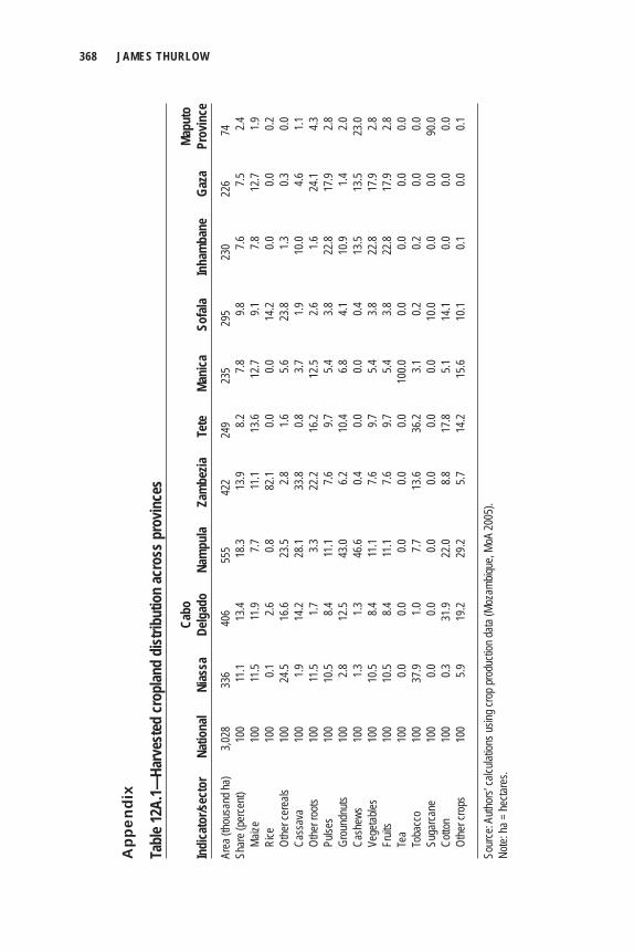
368 JAMES THURLOW
Tabl
e 12A
.1—Ha
rves
ted
crop
land
dist
ribut
ion
acro
ss p
rovin
ces
Ca
bo
Ma
puto
Indi
cato
r/sec
tor
Natio
nal
Nias
sa
Delg
ado
Nam
pula
Zam
bezia
Te
te
Mani
ca
Sofa
la In
ham
bane
Ga
za
Prov
ince
Area
(tho
usan
d ha)
3,0
28
336
406
555
422
249
235
295
230
226
74Sh
are (
perce
nt)
100
11.1
13.4
18.3
13.9
8.2
7.8
9.8
7.6
7.5
2.4
Maize
10
0 11
.5 11
.9 7.7
11
.1 13
.6 12
.7 9.1
7.8
12
.7 1.9
Ri
ce
100
0.1
2.6
0.8
82.1
0.0
0.0
14.2
0.0
0.0
0.2
Othe
r cer
eals
100
24.5
16.6
23.5
2.8
1.6
5.6
23.8
1.3
0.3
0.0
Cass
ava
100
1.9
14.2
28.1
33.8
0.8
3.7
1.9
10.0
4.6
1.1
Othe
r roo
ts 10
0 11
.5 1.7
3.3
22
.2 16
.2 12
.5 2.6
1.6
24
.1 4.3
Pu
lses
100
10.5
8.4
11.1
7.6
9.7
5.4
3.8
22.8
17.9
2.8
Grou
ndnu
ts 10
0 2.8
12
.5 43
.0 6.2
10
.4 6.8
4.1
10
.9 1.4
2.0
Ca
shew
s 10
0 1.3
1.3
46
.6 0.4
0.0
0.0
0.4
13
.5 13
.5 23
.0
Vege
tables
10
0 10
.5 8.4
11
.1 7.6
9.7
5.4
3.8
22
.8 17
.9 2.8
Fr
uits
100
10.5
8.4
11.1
7.6
9.7
5.4
3.8
22.8
17.9
2.8
Tea
100
0.0
0.0
0.0
0.0
0.0
100.0
0.0
0.0
0.0
0.0
To
bacc
o 10
0 37
.9 1.0
7.7
13
.6 36
.2 3.1
0.2
0.2
0.0
0.0
Su
garca
ne
100
0.0
0.0
0.0
0.0
0.0
0.0
10.0
0.0
0.0
90.0
Co
tton
100
0.3
31.9
22.0
8.8
17.8
5.1
14.1
0.0
0.0
0.0
Othe
r cro
ps
100
5.9
19.2
29.2
5.7
14.2
15.6
10.1
0.1
0.0
0.1
Sour
ce: A
uthor
s’ ca
lculat
ions u
sing c
rop p
rodu
ction
data
(Moz
ambiq
ue, M
oA 20
05).
Note:
ha =
hecta
res.
App
endi
x
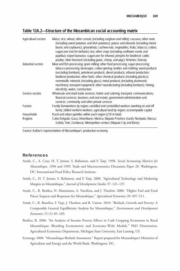
MOZAMBIQUE 369
Table 12A.2—Structure of the Mozambican social accounting matrix
Agricultural sectors Maize; rice; wheat; other cereals (including sorghum and millet); cassava; other roots (including sweet potatoes and Irish potatoes); pulses and oilseeds (including mixed
beans and soybeans); groundnuts; cashew nuts; vegetables; fruits; tobacco; cotton; sugarcane (not for biofuels); tea; other crops (including sunflower seeds and paprika); export bananas; sugarcane for ethanol; jatropha for biodiesel; cattle; poultry; other livestock (including goats, sheep, and pigs); fisheries; forestry
Industrial sectors Meat and fish processing; grain milling; other food processing; sugar processing; tobacco processing; beverages; cotton ginning; textiles and clothing; wood products
(excluding furniture); petroleum products; diesel products; ethanol production; biodiesel production; other fuels; other chemical products (including plastics); nonmetallic minerals (including glass); metal products (including aluminum); machinery; transport equipment; other manufacturing (including furniture); mining; electricity; water; construction
Service sectors Wholesale and retail trade services; hotels and catering; transport; communications; financial services; business and real estate; government administration and
services; community and other private servicesFactors Family farmworkers by region; unskilled and semiskilled workers (working on and off farm); skilled nonfarm workers; agricultural land by region; economywide capitalHouseholds Rural and urban quintiles within each region (210 in total)Regions Cabo Delgado; Gaza; Inhambane; Manica; Maputo Province (rural); Nampula; Niassa; Sofala; Tete; Zambezia; Metropolitan centers (Maputo City and Beira)
Source: Author’s representation of Mozambique’s production economy.
ReferencesArndt, C., A. Cruz, H. T. Jensen, S. Robinson, and F. Tarp. 1998. Social Accounting Matrices for
Mozambique, 1994 and 1995. Trade and Macroeconomics Discussion Paper 28. Washington,
DC: International Food Policy Research Institute.
Arndt, C., H. T. Jensen, S. Robinson, and F. Tarp. 2000. “Agricultural Technology and Marketing
Margins in Mozambique.” Journal of Development Studies 37: 121–137.
Arndt, C., R. Benfi ca, N. Maximiano, A. Nucifora, and J. Thurlow. 2008. “Higher Fuel and Food
Prices: Impacts and Responses for Mozambique.” Agricultural Economics 39: 497–511.
Arndt, C., R. Benefi ca, F. Tarp, J. Thurlow, and R. Uaiene. 2010. “Biofuels, Growth and Poverty: A
Computable General Equilibrium Analysis for Mozambique.” Environment and Development
Economics 15 (1): 81–105.
Benfi ca, R. 2006. “An Analysis of Income Poverty Effects in Cash Cropping Economies in Rural
Mozambique: Blending Econometric and Economy-Wide Models.” PhD Dissertation,
Agricultural Economics Department, Michigan State University, East Lansing, US.
Econergy. 2008. “Mozambique Biofuels Assessment.” Report prepared for Mozambique’s Ministries of
Agriculture and Energy and the World Bank, Washington, DC.
370 JAMES THURLOW
FAO (Food and Agriculture Organization of the United Nations). 2008. FAOSTAT Statistical Database.
Accessed September 16, 2011. http://faostat.fao.org/.
Heltberg, R., and F. Tarp. 2002. “Agricultural Supply Response and Poverty in Mozambique.” Food
Policy 27: 103–124.
Kyle, S. 1991. “Economic Reform and Armed Confl ict in Mozambique.” World Development 19 (6):
637–649.
McCool, C., J. Thurlow, and C. Arndt. 2009. “Documentation of Social Accounting Matrix (SAM)
Development.” In Taxation in a Low-Income Economy: The Case of Mozambique, edited by
C. Arndt and F. Tarp, 341–355. New York: Routledge.
Mozambique, MoA (Ministry of Agriculture). 2005. Trabalho de Inquerito Agricola 2005. Maputo,
Mozambique: Departments of Economics and Statistics.
Mozambique, MPD (Ministry of Planning and Development). 2010. Poverty and Well Being in
Mozambique: The Third National Assessment. Maputo, Mozambique: National Directorate of
Poverty Analysis and Studies.
Mozambique, NIS (National Institute of Statistics). 2004. Inquérito Nacional aos Agregados Familiares
Sobre Orçamento Familiar 2002/3. Maputo, Mozambique.
———. 2007. National Accounts: Commodity Supply and Use Tables and Sectoral Gross Domestic Product
Tables. Maputo, Mozambique.
Strasberg, P. 1997. “Smallholder Cash-Cropping, Food-Cropping and Food Security in Northern
Mozambique. PhD Dissertation, Agricultural Economics Department, Michigan State University,
East Lansing, US.
Tarp, F., C. Arndt, H. T. Jensen, S. Robinson, and R. Heltberg. 2002. Facing the Development Challenge
in Mozambique: An Economywide Perspective. Research Report 126. Washington, DC: International
Food Policy Research Institute.
Tschirley, D. L., and R. Benica. 2001. “Smallholder Agriculture, Wage Labour and Rural Poverty
Alleviation in Land-Abundant Areas of Africa: Evidence from Mozambique.” Journal of Modern
African Studies 39 (2): 333–358.
Tschirley, D. L., and M. T. Weber. 1994. “Food Security Strategies under Extremely Adverse Conditions:
The Determinants of Household Income and Consumption in Rural Mozambique.” World
Development 22 (2): 159–173.
Uaiene, R. 2008. “Determinants of Agricultural Technical Effi ciency and Technology Adoption in
Mozambique.” PhD Dissertation, Center for Global Trade Analysis, Purdue University, West
Lafayette, IN, US.
World Bank. 2010. World Development Indicators. Washington, DC.
C h a p t e r 1 3
TanzaniaKarl Pauw and James Thurlow
Despite its poor performance during the 1980s and 1990s, Tanzania’s economy expanded rapidly after the turn of the century, with national gross domes-tic product (GDP) growing at 6.6 percent per year during 1998 –2007
(Tanzania, MFEA 2008). This rate was almost double the average growth rate achieved in the previous decade; between 1990 and 1995 the recorded growth was only 2.7 percent, after which it steadily improved to reach 5 percent per year by 2000. Recent economic growth also appears to have been relatively broadly based. Although the newly established gold-mining sector recorded the highest growth rates during 1998–2007, it was the large agriculture and manufacturing sectors that contributed the most to national growth.
Despite Tanzania’s high and seemingly broadly based economic growth, house-hold income poverty has remained virtually unchanged. The national poverty headcount fell only 2.1 percentage points (from 35.7 percent in 2000/01 to 33.6 percent in 2007), with equally modest declines in rural and urban areas (World Bank 2009). In comparison, poverty declined by about 2 percentage points between 1992 and 2000, despite signifi cantly lower economic growth at the time (Treichel 2005). Economic growth therefore appears to have little effect on poverty in Tanzania. Moreover, its impact on poverty seems to have become weaker over time. This trend raises concerns over a possible decoupling of economic growth and poverty reduction in Tanzania. Moreover, the household surveys fi nd that income inequality did not change signifi cantly during 2001–07 (World Bank 2009). Although this may suggest an inconsistency between the growth reported in national accounts and the poverty and inequality changes reported in the household surveys, the weak poverty–growth relationship remains a concern that underlines the need
372 KARL PAUW AND JAMES THURLOW
to better understand the poverty and distributional consequences of alternative sources of growth.
Along with persistent income poverty, Tanzania also suffers from high levels of malnutrition. About 17 percent of children are underweight, and 4 out of every 10 children are stunted (World Bank 2007, 2008). Recent trends suggest that even though average per capita agricultural GDP expanded rapidly during 1998–2007, caloric availability at the household level hardly improved. For example, estimates based on the two latest household surveys show that the share of people who had insuffi cient calories available to them fell only slightly, from about 25.0 to 23.5 percent, between 2001 and 2007 (World Bank 2009). Thus, rising farm and national incomes have little effect on households’ access to food, ability to acquire food, or both; and it raises further concerns about a possible disconnect between agricultural growth and nutritional outcomes.
Tanzania’s development outcomes over the past decade raise three questions:
1. Is the level and structure of the current economic growth path consistent with the slow decline in national poverty and only modest improvement in house-holds’ caloric availability?
2. What is the contribution of agriculture in reducing poverty and raising caloric availability?
3. Which agricultural subsectors are most effective at achieving national growth, poverty reduction, and nutrition objectives?
We address these questions using a dynamic computable general equilibrium (DCGE) model for Tanzania, as described in Chapter 2 of this volume. A micro-simulation model is linked sequentially to the DCGE model to measure how changes in economic growth affect both household poverty and the availability of calories in households. This combination of poverty and nutrition modules and a focus on these joint outcomes is a unique feature of the Tanzanian case study.
This chapter is organized as follows. We fi rst look at the recent growth perfor-mance of the Tanzanian economy and consider the impact of structural adjustment policies on growth and development in the agricultural sector in particular. We then briefl y discuss the structure of the Tanzanian DCGE model, its underlying data sources, and the accompanying microsimulation models used to evaluate poverty and nutritional impacts at the household level. Model results are presented for a baseline scenario and an accelerated growth scenario. Finally, agricultural subsectors that are most effective at generating economic growth, reducing income poverty, and improving nutrition in Tanzania are identifi ed. The fi nal section draws together
TANZANIA 373
the main fi ndings and identifi es policy options for realizing agricultural growth, poverty reduction, and nutrition objectives.
Agriculture in Tanzania
Agricultural Performance under Structural AdjustmentTanzania’s growth path over the past decades is best evaluated in the context of the structural adjustment policies introduced during the 1980s. After the weak perfor-mance of the economy during the 1970s—ascribed largely to internal factors, such as the highly monopolized state-run banking system, a large and ineffi cient govern-ment sector, and government control over domestic prices and the exchange rate (Meertens 2000)—a period of structural adjustment followed in the 1980s. The structural adjustment program provided for an increased role of markets and is generally praised for the role it played in bringing about macroeconomic and price stability (Treichel 2005). This stability allowed the Tanzanian economy to shift to a higher growth plane. However, the gains did not extend to the agricultural sector as much as was hoped for, with agricultural output per capita stagnating or even falling throughout the 1990s (Danielson 2002).
Various factors have contributed to the urban bias created by the structural adjustment program. One of the important early outcomes of structural adjustment and the overall deregulation that accompanied it was a sharp depreciation of the Tanzanian currency toward the end of the 1980s. Although a weaker currency was potentially benefi cial to agricultural exporters, it also meant that the cost of inter-mediate inputs, many of which were (and still are) imported, such as fertilizers and agricultural machinery, increased rapidly. This resulted in a sharp decrease in fertil-izer use—an effect compounded by the removal of government input subsidies—and an overall demechanization of agriculture (Meertens 2000). Reduced fertilizer use is considered one of the main causes of declining agricultural yields, and reduced productivity further counteracted potential gains from the currency depreciation (Danielson 2002). Moreover, as domestic crop prices remained stagnant, those producing for the local market faced a cost–price squeeze; for example, Morris et al. (2007) cite evidence that fertilizer–crop price ratios more than doubled in such countries as Tanzania between 1980 and the mid-1990s. With rapidly deteriorating profi ts, there was little or no incentive to invest in agriculture.
Under structural adjustment Tanzania’s government steadily reduced direct support for agriculture, which left a void that the private sector was unwilling or unable to fi ll. Especially for farmers who were geographically isolated, deregulation and the “receding presence of institutional credit and crop purchases at guaranteed, territorially uniform prices meant times were harder than ever” (Putterman 1995,
374 KARL PAUW AND JAMES THURLOW
321). This situation, together with a weak physical infrastructure in the country, led to structural bottlenecks in agricultural supply, which explains the low or even nega-tive agricultural supply elasticities at the time (Danielson 2002).
Tanzania’s agricultural sector remains fairly traditional, with little use of modern inputs and farming practices. Farmers are reluctant to adopt improved seed varieties (for example, drought-resistant species) because of low market and consumption values and the high labor investment associated with their cultivation (Eriksen 2001). The Minister of Agriculture, Food Security and Cooperatives in Tanzania recently stated that 90 percent of farmers still use low-productivity recycled seeds, which he ascribed to weak extension services, a lack of credit, and high seed prices stemming from the ineffi cient and underdeveloped seed distribution and marketing system (African Agriculture 2008). Additionally, less than 1 percent of land suited to it is currently under irrigation (JGDPG 2009). Where irrigation systems do exist, they are costly to maintain and are underdeveloped, especially in poor communities (Mmbaga and Lyamchai 2001). Changing farming practices have also played a role. Whereas historically the traditional agricultural method of fallow and rotation was followed in Tanzania, population growth, rural–urban migration, and increased export opportunities have led to the adoption of persistent-farming practices (Wiig et al. 2001). On many farms soils are no longer allowed to recuperate naturally, which means that erosion and nutrient depletion are pervasive. This degradation is aggravated when nutrients are not replaced artifi cially using organic and mineral fertilizers.
In contrast to an overall economic growth rate of about 7 percent since 2002, agricultural growth has been volatile and weak relative to that of other sectors, fl uctuating between 3 and 6 percent annually since 2000 (JGDPG 2009). At the subsector level, however, there are some success stories. Table 13.1 evaluates the structure of crop production in Tanzania more closely. More than half of total har-vested land area is allocated to cereals, of which maize is the country’s dominant staple foodcrop produced mainly by subsistence smallholders. Despite its favorable agroecological conditions, Tanzania is a net importer of cereals. Maize yields are typically low (0.88 tons per hectare), given the constraints discussed above. In con-trast, wheat is produced almost exclusively by large-scale commercial farmers in the Northern zone using modern inputs. Growth in cereal production varies greatly by crop (FAO 2009). Maize production expanded slower than the overall population during 2000–07, implying declining per capita production. In contrast, wheat and rice grew rapidly during the same period, with rice becoming a particularly impor-tant crop for smallholder farmers in the Western and Lake zones (Tanzania, MAFSC 2006) and an important food source for higher income households (World Bank 2009). Indeed, even the rapid expansion of rice and wheat production has failed to keep pace with rising consumer demand, causing imports to rise. Thus, it was rice
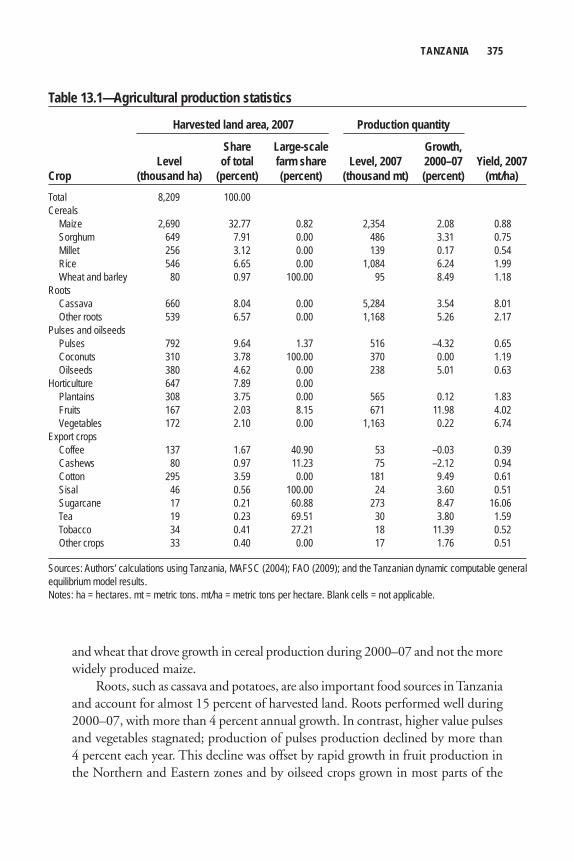
TANZANIA 375
and wheat that drove growth in cereal production during 2000–07 and not the more widely produced maize.
Roots, such as cassava and potatoes, are also important food sources in Tanzania and account for almost 15 percent of harvested land. Roots performed well during 2000–07, with more than 4 percent annual growth. In contrast, higher value pulses and vegetables stagnated; production of pulses production declined by more than 4 percent each year. This decline was offset by rapid growth in fruit production in the Northern and Eastern zones and by oilseed crops grown in most parts of the
Table 13.1—Agricultural production statistics
Harvested land area, 2007 Production quantity
Share Large-scale Growth, Level of total farm share Level, 2007 2000–07 Yield, 2007Crop (thousand ha) (percent) (percent) (thousand mt) (percent) (mt/ha)Total 8,209 100.00 Cereals Maize 2,690 32.77 0.82 2,354 2.08 0.88 Sorghum 649 7.91 0.00 486 3.31 0.75 Millet 256 3.12 0.00 139 0.17 0.54 Rice 546 6.65 0.00 1,084 6.24 1.99 Wheat and barley 80 0.97 100.00 95 8.49 1.18Roots Cassava 660 8.04 0.00 5,284 3.54 8.01 Other roots 539 6.57 0.00 1,168 5.26 2.17Pulses and oilseeds Pulses 792 9.64 1.37 516 –4.32 0.65 Coconuts 310 3.78 100.00 370 0.00 1.19 Oilseeds 380 4.62 0.00 238 5.01 0.63Horticulture 647 7.89 0.00 Plantains 308 3.75 0.00 565 0.12 1.83 Fruits 167 2.03 8.15 671 11.98 4.02 Vegetables 172 2.10 0.00 1,163 0.22 6.74Export crops Coffee 137 1.67 40.90 53 –0.03 0.39 Cashews 80 0.97 11.23 75 –2.12 0.94 Cotton 295 3.59 0.00 181 9.49 0.61 Sisal 46 0.56 100.00 24 3.60 0.51 Sugarcane 17 0.21 60.88 273 8.47 16.06 Tea 19 0.23 69.51 30 3.80 1.59 Tobacco 34 0.41 27.21 18 11.39 0.52 Other crops 33 0.40 0.00 17 1.76 0.51
Sources: Authors’ calculations using Tanzania, MAFSC (2004); FAO (2009); and the Tanzanian dynamic computable general equilibrium model results.Notes: ha = hectares. mt = metric tons. mt/ha = metric tons per hectare. Blank cells = not applicable.
376 KARL PAUW AND JAMES THURLOW
country. Noncereal foodcrop production has therefore been characterized by slow growth in the more widely produced pulses and vegetables, and fast growth in more regionally concentrated fruits.
Some of the fastest growth rates during 2000–07 were for export crops. Traditional crops, such as cotton, sugarcane, and tobacco, grew by almost 10 percent per year. These crops are highly concentrated in specifi c regions. Cotton is mostly produced by smallholders in the Western and Lake zones (81.5 percent of output). Tobacco, another smallholder crop, is mainly produced in the Western and Highlands zones (82.8 percent). Finally, sugarcane is mostly produced by large-scale commercial farmers in the Eastern and Northern zones (83.8 percent). Together, these three crops generated 17.4 percent of total merchandize exports in 2007. Export agriculture therefore grew rapidly during 2000–07, driven by the strong performance of a few regionally concentrated crops.
Finally, livestock and fi sheries are key subsectors, accounting for almost one-third of agricultural GDP. Fisheries kept pace with overall agricultural production during 1998–2007, growing at 5.1 percent per year. However, livestock has lagged behind crop agriculture, growing at only 3.3 percent per year. Incomes from cattle and poultry are important for farm livelihoods in many parts of the country, espe-cially for low-income households (World Bank 2009). Thus, their slow growth will have implications for households’ incomes, especially for the poor.
In conclusion, the examination of recent production trends suggest that although the agricultural sector as a whole performed reasonably well between 2000 and 2007, the source of this growth has been concentrated among a few crops. Rice and wheat, for example, dominate cereal production trends, and cotton, tobacco, and sugar grew at almost 10 percent per year. These well-performing crops are more heavily concentrated in the northern and eastern periphery of the country and are more often produced by large-scale commercial farmers. Agricultural growth has therefore not benefi ted those who are most likely to be poor, such as subsistence farmers.
Agricultural Growth Potential Tanzania’s Minister of Agriculture, Food Security and Cooperatives thinks that the current agricultural growth rate of 3–6 percent is insuffi cient, arguing that it should be closer to 10 percent if the country is to reach its Millennium Development Goals (African Agriculture 2008). This growth rate would require substantial improve-ments in agricultural productivity and more effective land use. Given the under-utilization of resources, policymakers are optimistic that such a high level of agricultural growth is attainable. For example, only 23 percent of arable land is cur-rently used for agricultural production; there is large scope for expanding irrigation, and many freshwater resources remain underutilized; and livestock production is
TANZANIA 377
not yet commercially exploited. The government has therefore identifi ed the agri-cultural sector as a future engine of growth; given the sector’s potential to reduce poverty, the transformation of agriculture is regarded as the foundation of the coun-try’s socioeconomic development plan (JGDPG 2009).
There is still debate about which types of interventions should enjoy priority. The Tanzanian government seems intent on investing heavily in irrigation (see Wolter 2008; Malley, Taeb, and Matsumoto 2009), but the Ministry of Agriculture, Food Security and Cooperatives also realizes the importance of the use of modern inputs, which could be achieved through the provision of improved extension ser-vices by the government (African Agriculture 2008). The adoption of drought-resistant crops and technologies is already an explicit priority in certain Tanzanian districts (Eriksen 2001); the success of smart input subsidies in neighboring Malawi has prompted Tanzania to adopt a similar voucher-based program (Sanchez, Denning, and Nziguheba 2009). The distribution of inputs, however, remains a constraint. In 2003, for example, Tanzania only had 300 input dealers, mostly located in urban and semiurban areas. Smallholder farmers therefore have to travel long distances, on average about 20–30 km, to purchase fertilizer (Morris et al. 2007).
Malley, Taeb, and Matsumoto (2009) agree that improved fertilizer application is required to raise soil productivity, but they stress the importance of combining policies that promote fertilizer use with programs that educate farmers about sus-tainable use and management of land resources. The benefi ts of conservation farm-ing techniques are well documented in Tanzania and elsewhere. For example, trials show that during dry years crop yields using conservation farming methods are two to three times higher than those obtained using traditional methods (Mmbaga and Lyamchai 2001).
Although on-farm reforms are important, Wolter (2008) insists that they will only yield results if the three classic constraints to agricultural growth—infrastructure, fi nancial services, and land rights—are addressed simultaneously. Thus, rural roads, storage facilities, and the accessibility of ports and airports should be improved; access to credit needs to be improved by reforming the almost nonexistent banking sector; and land rights and ownership issues need to be addressed to attract large-scale agricultural investments, especially from abroad (Wolter 2008).
A review of the literature cited here suggests a great deal of consensus that the withdrawal of government under structural adjustment went too far in Tanzania. Meertens (2000) calls for a modifi cation of structural adjustment, arguing that the cost of subsidizing agriculture will be a better investment in food security than hav-ing to import food, as is currently the case. Investment in agricultural research and development in Africa has been associated with returns in excess of 20 percent (see Thirtle, Lin, and Piesse 2003). In Tanzania, such investments are bound to pay off. For example, Fan, Nyanga, and Rao (2005) show that investing in research and
378 KARL PAUW AND JAMES THURLOW
extension in Tanzania has large positive impacts on agricultural growth and house-hold incomes. The econometric estimates of Fan, Nyanga, and Rao (2005) suggest that every 1 million Tanzanian shillings (TZS) spent on agricultural research (in 1999 prices) increases household incomes by TZS12.5 million and lifts 40 people above the poverty line. Moreover, the returns to agricultural research are found to have higher impacts than similar investments in education and rural roads, both of which also have positive returns.
Despite these high expected returns, budgetary allocations to agriculture aver-aged only 3 percent of the total budget during 2004–07. This share has also deterio-rated over time (Tanzania, MFEA 2008). Moreover, spending on research and extension comprises less than 15 percent of the agricultural budget. The Tanzanian government’s renewed focus on agriculture as a driver of growth and socioeconomic development is hopefully an indication of a turnaround in these trends. Without such a policy shift Tanzania’s agricultural growth potential is unlikely to be realized.
The Tanzanian DCGE Model and Nutrition ModuleThe Tanzanian DCGE model is calibrated with a 2007 social accounting matrix (SAM). The SAM includes 58 sectors, half of which are in agriculture and agro-processing (see Table 13A.1 in the appendix to this chapter). Agricultural sectors are further disaggregated into 20 subnational regions, which for reporting purposes here are grouped into eight agricultural zones. The model also distinguishes between small- and large-scale farmers. This spatial dimension of the model captures different crop-ping patterns and agroecological conditions in the country. Data on crop production and livestock are from the 2002/03 agricultural sample census (Tanzania, MAFSC 2004, 2006). Nonagricultural production and employment data were compiled from the 2000/01 Household Budget Survey (HBS) (Tanzania, NBI 2002). On the demand side, information on industrial technologies (such as intermediate and factor demands) was taken from an earlier SAM for Tanzania (Thurlow and Wobst 2003).
The SAM identifi es 110 different household groups. Rural farm households are disaggregated into the 20 subnational regions and fi ve income quintiles. The model also distinguishes rural and urban nonfarm households, each disaggregated into income quintiles. Income and expenditure patterns and income elasticities for the various household groups were estimated using HBS 2000/01. The model in-cludes 58 commodities. To improve results at the microlevel, the DCGE model is linked to a microsimulation model used to produce poverty and improve nutrition results at the individual household level.
As described in Chapter 2 of this volume, the poverty module measures the change in the incidence of poverty by linking changes in the value of some aggregate
TANZANIA 379
measure of consumption observed for each of the household groups in the DCGE model to the individual households in the microsimulation model. In general, the strength of the poverty–growth relationship depends on the structure of growth and how the poor are linked to various economic sectors or subsectors via consumption and employment (Ravallion and Datt 1996; Mellor 1999). Poor people in develop-ing countries typically derive a large share of their incomes from agricultural activi-ties or allocate a large share of their budgets to food consumption, or both. Thus, agricultural productivity growth has the potential to reduce poverty via both income and consumption channels (Diao, Hazell, and Thurlow 2010). However, even agricultural productivity growth may not effectively reduce poverty if it is not con-centrated in those regions or subsectors where resource-poor farmers are typically located, or if it is driven by growth in subsectors that produce goods not consumed intensively by the poor (for example, export products). To understand the effect of growth on poverty, it may therefore be necessary to focus on subsector growth patterns.
Growth affects nutrition in much the same way as it does poverty. The growth–nutrition relationship is, however, more complex than the poverty–growth relation-ship. Poverty analyses typically consider utility derived from a broad range of consumption items, whereas nutrients are only derived from food consumption. When growth causes incomes to rise, nutrition generally improves, as households are able to purchase more or better foods (Timmer 1988). However, because differ-ent food types have different nutritional attributes, it is also necessary to consider how growth-induced income and relative changes in food prices affect households’ food consumption baskets. For example, if the price of calorie-rich maize increases and that of protein-rich meat declines so that the overall food price index is unchanged, the calorie defi ciency rate might decline and the protein defi ciency rate might increase, even though the poverty rate remains unchanged.
Many studies on nutrition or food demand focus on food energy (calories), where caloric availability is estimated from household expenditure surveys (hence the term “caloric availability” as opposed to “intake”). Although other macro- and micronutrients are important, a narrow focus on caloric availability is perhaps justi-fi ed by the spending preferences of poor consumers, who allocate a large share of their incomes to calorie-rich food types, mainly to avoid feeling hungry (Ecker 2009). Calorie-rich food types are also often more abundant and cost less per calorie than other food types. Policies that lower the cost of these calorie-rich foods relative to others may therefore have a signifi cant impact on caloric intake. To illustrate, Table 13.2 compares calorie contents across different food types in Tanzania. The table also shows how the price per 100 kilocalories varies across these products. For example, livestock products have higher calorie contents per 100-gram serving compared to most other food types, but the higher price of animal products means
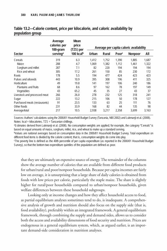
380 KARL PAUW AND JAMES THURLOW
that they are ultimately an expensive source of energy. The remainder of the columns show the average number of calories that are available from different food products for urban/rural and poor/nonpoor households. Because per capita incomes are fairly low on average, it is unsurprising that a large share of daily calories is obtained from foods with low prices per calorie, particularly the staple maize. The share is slightly higher for rural/poor households compared to urban/nonpoor households, given welfare differences between these household subgroups.
Looking only at income changes and how they affect household access to food, as partial equilibrium analyses sometimes tend to do, is inadequate. A comprehen-sive analysis of growth and nutrition should also focus on the supply side (that is, food availability), preferably within an integrated framework. A general equilibrium framework, through combining the supply and demand sides, allows us to consider both the access and availability dimensions of food security and nutrition. Prices are endogenous in a general equilibrium system, which, as argued earlier, is an impor-tant demand-side consideration in nutrition analyses.
Table 13.2—Calorie content, price per kilocalorie, and caloric availability by population group
Average Mean calories per price 100-gram (TZS) perSector servinga 100 kcalb Urban Rural Poorc Nonpoor AllCereals 319 6.3 1,412 1,752 1,390 1,885 1,687 Maize 288 4.7 1,069 1,382 1,112 1,461 1,322 Sorghum and millet 287 7.1 82 220 194 194 194 Rice and wheat 305 17.2 261 150 85 230 172Roots 178 5.5 194 477 424 423 423Pulses and oilseeds 443 10.9 395 308 196 411 325Horticulture 49 19.8 141 197 106 240 186 Plantains and fruits 68 8.6 97 162 78 197 149 Vegetables 43 65.2 45 35 27 43 37Livestock and processed meat 266 26.0 278 232 125 318 241Sugar 222 13.2 215 106 50 178 127Purchased meals (restaurants) 91 23.5 133 63 25 111 76Other foods 231 33.9 168 82 44 135 98Average/total 217 10.5 2,938 3,217 2,358 3,699 3,163
Sources: Authors’ calculations using the 2000/01 Household Budget Survey (Tanzania, NBI 2002) and Lukmanji et al. (2008). Notes: kcal = kilocalories. TZS = Tanzanian shillings.aEstimates derived from Lukmanji et al. (2008). No consumption weights are applied; for example, the category “Cereals” is based on equal amounts of maize, sorghum, millet, rice, and wheat to make up a standard serving. bValues are national averages based on consumption data in the 2000/01 Household Budget Survey. Total expenditure on different food items is divided by the calorie content; that is, consumption weights do come into play. cThe poverty line is defined as the 40th percentile of per capita expenditure (as reported in the 2000/01 Household Budget Survey), so that the bottom two expenditure quintiles of the population are defined as poor.
Average per capita caloric availability
TANZANIA 381
The nutrition module operates in much the same way as the poverty module: consumption results for different household groups are linked to individual house-holds in the microsimulation model. The microsimulation model draws on food consumption data from HBS 2000/01 and caloric content tables from Lukmanji et al. (2008) to calculate initial household caloric availability. The DCGE model results on changes in food consumption quantities (not values) are then applied to the survey data to estimate changes in household caloric availability. We compare both the original and new levels of caloric availability against a “malnutrition line” of 2,550 kilocalories (per male adult equivalent) to determine changes in calorie-defi ciency rates. Equivalence scales are from UNU, WHO, and FAO (2004). Thus, both the size and demographic structure of households determine the minimum number of calories required by each household.
Baseline Growth ScenarioTable 13.3 shows the observed production growth rates for 2000–07 and modeled growth rates in the baseline scenario. Taking maize as an example, national pro-duction in the baseline scenario grows at 2.11 percent per year during 2009–15, which is similar to the 2.08 annual growth rate observed during 2000–07. This increase is partly achieved by allowing total harvested land area in Tanzania to expand by 2 percent per year during 2009–15. The model endogenously allocates available land in each of the 20 regions across crops to maximize returns. We then exogenously increase total factor productivity (TFP) for each crop and region to achieve the targeted production growth rate. This increase causes cropland yields to change. For example, maize yields rise from 0.91 to 1.02 tons per hectare dur-ing 2009–15 in the baseline scenario (that is, the annual yield growth rate is 1.45 percent, as shown in the table). This process of targeting production trends is repeated for each crop and livestock subsector. We also target nonagricultural sector GDP growth rates using trends from national accounts for 1998–2007 (Tanzania, MFEA 2008).
Table 13.4 shows average annual agricultural GDP growth after replicating crop-level production trends. The agricultural GDP growth rate is 4 percent in the baseline scenario for 2009–15. This suggests that the agricultural growth rate reported in national accounts for 1998–2007 (4.4 percent) is broadly consistent with subsector production trends. Crop agriculture’s GDP growth rate, for example, grows at 4.23 percent per year in the baseline scenario, compared with the observed 4.76 percent growth rate reported in national accounts. Thus, in line with recent trends, agricultural growth in the baseline scenario is driven by strong growth in crop agriculture and more modest growth in livestock. National economic growth, however, is driven by a rapid expansion of industry and services. Manufacturing is partly constrained by slower agricultural growth, which limits upstream food pro-
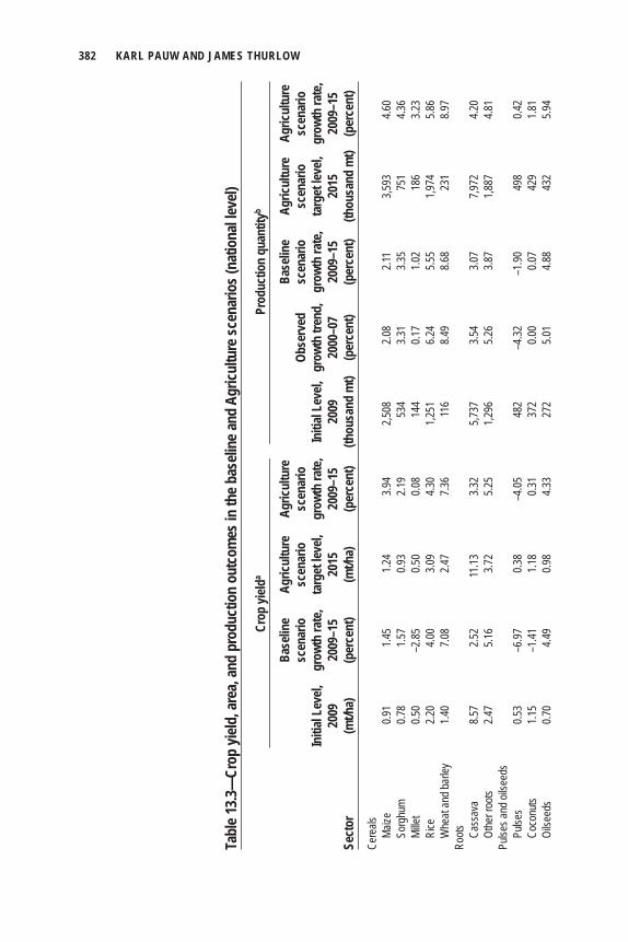
382 KARL PAUW AND JAMES THURLOW
Tabl
e 13.3
—Cr
op yi
eld, a
rea,
and
prod
uctio
n ou
tcom
es in
the b
aseli
ne an
d Ag
ricul
ture
scen
ario
s (na
tiona
l leve
l)
Cr
op yi
elda
Prod
uctio
n qu
antit
yb
Base
line
Agric
ultu
re
Agric
ultu
re
Base
line
Agric
ultu
re
Agric
ultu
re
sc
enar
io
scen
ario
sc
enar
io
Ob
serv
ed
scen
ario
sc
enar
io
scen
ario
In
itial
Leve
l, gr
owth
rate
, ta
rget
leve
l, gr
owth
rate
, In
itial
Leve
l, gr
owth
tren
d,
grow
th ra
te,
targ
et le
vel,
grow
th ra
te,
20
09
2009
–15
2015
20
09–1
5 20
09
2000
–07
2009
–15
2015
20
09–1
5Se
ctor
(m
t/ha)
(p
erce
nt)
(mt/h
a)
(per
cent
) (th
ousa
nd m
t) (p
erce
nt)
(per
cent
) (th
ousa
nd m
t) (p
erce
nt)
Cere
als
Ma
ize
0.91
1.45
1.24
3.94
2,508
2.0
8 2.1
1 3,5
93
4.60
So
rghu
m 0.7
8 1.5
7 0.9
3 2.1
9 53
4 3.3
1 3.3
5 75
1 4.3
6
Mille
t 0.5
0 –2
.85
0.50
0.08
144
0.17
1.02
186
3.23
Ri
ce
2.20
4.00
3.09
4.30
1,251
6.2
4 5.5
5 1,9
74
5.86
W
heat
and b
arley
1.4
0 7.0
8 2.4
7 7.3
6 11
6 8.4
9 8.6
8 23
1 8.9
7Ro
ots
Cass
ava
8.57
2.52
11.13
3.3
2 5,7
37
3.54
3.07
7,972
4.2
0
Othe
r roo
ts 2.4
7 5.1
6 3.7
2 5.2
5 1,2
96
5.26
3.87
1,887
4.8
1Pu
lses a
nd oi
lseed
s
Pu
lses
0.53
–6.97
0.3
8 –4
.05
482
–4.32
–1
.90
498
0.42
Co
conu
ts 1.1
5 –1
.41
1.18
0.31
372
0.00
0.07
429
1.81
Oi
lseed
s 0.7
0 4.4
9 0.9
8 4.3
3 27
2 5.0
1 4.8
8 43
2 5.9
4
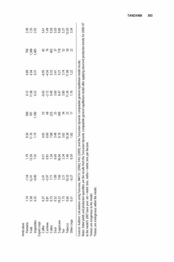
TANZANIA 383
Hortic
ultur
e
Pl
antai
ns
1.74
–1.54
1.7
9 0.3
0 58
0 0.1
2 0.8
9 70
6 2.4
9
Fruit
s 5.5
8 12
.41
13.59
11
.76
787
11.98
6.9
4 1,3
88
7.35
Ve
getab
les
6.55
–0.80
7.5
5 1.7
9 1,1
80
0.22
0.37
1,485
2.9
2Ex
port
crops
Co
ffee
0.37
–2.41
0.5
1 4.0
5 53
–0
.03
–0.95
82
5.6
1
Cash
ews
0.81
–5.97
0.8
1 0.0
0 68
–2
.12
–4.56
76
1.4
9
Cotto
n 0.7
3 7.7
1 1.3
4 7.8
8 22
5 9.4
9 9.3
3 46
5 9.5
0
Sisa
l 0.5
2 1.8
9 0.6
9 3.4
8 25
3.6
0 3.4
1 37
5.0
3
Suga
rcane
19
.22
7.66
36.04
8.1
8 34
0 8.4
7 9.2
7 71
8 9.8
0
Tea
1.73
2.21
2.34
3.82
34
3.80
3.74
52
5.37
To
bacc
o 0.6
6 10
.33
1.46
10.38
23
11
.39
11.98
58
12
.03
Othe
r cro
ps
0.51
–0.27
0.5
9 1.8
2 17
1.7
6 1.2
2 22
3.3
4
Sour
ces:
Autho
rs’ ca
lculat
ions u
sing T
anza
nia, M
AFSC
(200
6); F
AO (2
009)
; and
the T
anza
nian d
ynam
ic co
mputa
ble ge
nera
l equ
ilibriu
m mo
del re
sults
. No
tes: In
itial y
ields
and p
rodu
ction
quan
tities
are t
he re
sults
from
the T
anza
nian d
ynam
ic co
mputa
ble ge
nera
l equ
ilibriu
m mo
del a
fter a
pplyi
ng ob
serve
d pro
ducti
on tr
ends
for 2
000–
07
to the
mod
el’s 2
007 b
ase y
ear. m
t = m
etric
tons.
mt/ha
= m
etric
tons p
er he
ctare
.a Va
lues a
re ex
ogen
ous t
o the
mod
el.b Va
lues a
re en
doge
nous
with
in the
mod
el.
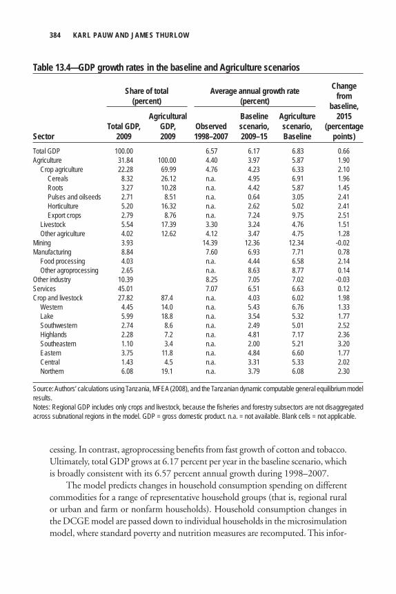
384 KARL PAUW AND JAMES THURLOW
cessing. In contrast, agroprocessing benefi ts from fast growth of cotton and tobacco. Ultimately, total GDP grows at 6.17 percent per year in the baseline scenario, which is broadly consistent with its 6.57 percent annual growth during 1998–2007.
The model predicts changes in household consumption spending on different commodities for a range of representative household groups (that is, regional rural or urban and farm or nonfarm households). Household consumption changes in the DCGE model are passed down to individual households in the microsimulation model, where standard poverty and nutrition measures are recomputed. This infor-
Table 13.4—GDP growth rates in the baseline and Agriculture scenarios
Change from baseline, Agricultural Baseline Agriculture 2015 Total GDP, GDP, Observed scenario, scenario, (percentageSector 2009 2009 1998–2007 2009–15 Baseline points)Total GDP 100.00 6.57 6.17 6.83 0.66Agriculture 31.84 100.00 4.40 3.97 5.87 1.90 Crop agriculture 22.28 69.99 4.76 4.23 6.33 2.10 Cereals 8.32 26.12 n.a. 4.95 6.91 1.96 Roots 3.27 10.28 n.a. 4.42 5.87 1.45 Pulses and oilseeds 2.71 8.51 n.a. 0.64 3.05 2.41 Horticulture 5.20 16.32 n.a. 2.62 5.02 2.41 Export crops 2.79 8.76 n.a. 7.24 9.75 2.51 Livestock 5.54 17.39 3.30 3.24 4.76 1.51 Other agriculture 4.02 12.62 4.12 3.47 4.75 1.28Mining 3.93 14.39 12.36 12.34 -0.02Manufacturing 8.84 7.60 6.93 7.71 0.78 Food processing 4.03 n.a. 4.44 6.58 2.14 Other agroprocessing 2.65 n.a. 8.63 8.77 0.14Other industry 10.39 8.25 7.05 7.02 -0.03Services 45.01 7.07 6.51 6.63 0.12Crop and livestock 27.82 87.4 n.a. 4.03 6.02 1.98 Western 4.45 14.0 n.a. 5.43 6.76 1.33 Lake 5.99 18.8 n.a. 3.54 5.32 1.77 Southwestern 2.74 8.6 n.a. 2.49 5.01 2.52 Highlands 2.28 7.2 n.a. 4.81 7.17 2.36 Southeastern 1.10 3.4 n.a. 2.00 5.21 3.20 Eastern 3.75 11.8 n.a. 4.84 6.60 1.77 Central 1.43 4.5 n.a. 3.31 5.33 2.02 Northern 6.08 19.1 n.a. 3.79 6.08 2.30
Source: Authors’ calculations using Tanzania, MFEA (2008), and the Tanzanian dynamic computable general equilibrium model results. Notes: Regional GDP includes only crops and livestock, because the fisheries and forestry subsectors are not disaggregated across subnational regions in the model. GDP = gross domestic product. n.a. = not available. Blank cells = not applicable.
Share of total (percent)
Average annual growth rate(percent)
TANZANIA 385
mation is used to calculate poverty– and calorie–growth elasticities, which are compared against their initial levels.
The poverty−growth elasticity is defi ned as the percentage decline in poverty resulting from a 1 percent increase in per capita GDP. This elasticity may be sensitive to whether the per capita GDP estimate is derived from household survey data or from the national accounts. Private consumption, a key component of GDP, is typi-cally larger in national accounts compared to household surveys, because it includes a wider range of products and also because surveys are less likely to sample house-holds at the top of the income distribution. National account estimates are further prone to error because private consumption is treated as a residual between GDP at factor cost and other components of GDP at market prices rather than measured directly (see Ravallion 2001). Over time, discrepancies may widen, and so house-hold surveys can provide a check on consumption trends in national accounts.
Tanzania’s national accounts suggest that per capita GDP grew by 3.99 percent per year during 2001–07. This rate is well above the 1.32 percent estimated from the household surveys. Poverty as measured in the household survey declined by 1.01 percent per year during the same period; hence, the poverty–growth elasticity may have been as low as 0.25, based on national accounts estimates of GDP, or 0.76 if per capita consumption levels from the household surveys are used. The estimates based on national accounts further suggest a deterioration of the poverty–growth relationship from 0.82 during the 1990s to 0.25 during the 2000s, whereas the household surveys suggest the opposite (an increase from 0.57 to 0.76). Under-standing these differences is important, because they imply different trends in the effectiveness of economic growth to reduce poverty.
Similarly, we defi ne the calorie–growth elasticity as the percentage change in the calorie defi ciency rate (that is, the share of the population below the calorie line of 2,550 kilocalories per day per adult male equivalent) divided by the percentage change in per capita GDP. The calorie defi ciency rate dropped by 1.03 percent per year (from 25.0 to 23.5 percent) (World Bank 2009). The calorie–growth elasticity range is therefore very similar to that for the poverty–growth elasticity (0.26–0.78). In contrast to the normal calorie–income elasticity, which considers changes in average caloric availability across the entire population, the calorie–growth elasticity is sensitive to growth-induced changes in caloric availability in households close to the calorie defi ciency line only.
The Tanzanian model estimates that, in the baseline scenario, the increase in average per capita GDP by 3.59 percent each year (assuming 2.5 percent population growth) will cause the national poverty headcount to decline from 40.0 percent in 2007 to 31.1 percent by 2015 (Table 13.5). This is a 3.09 percent annual decline in the poverty rate and so implies a poverty–growth elasticity of 0.86 (3.09 divided by 3.59). This value is slightly above the 0.76 poverty–growth elasticity estimated
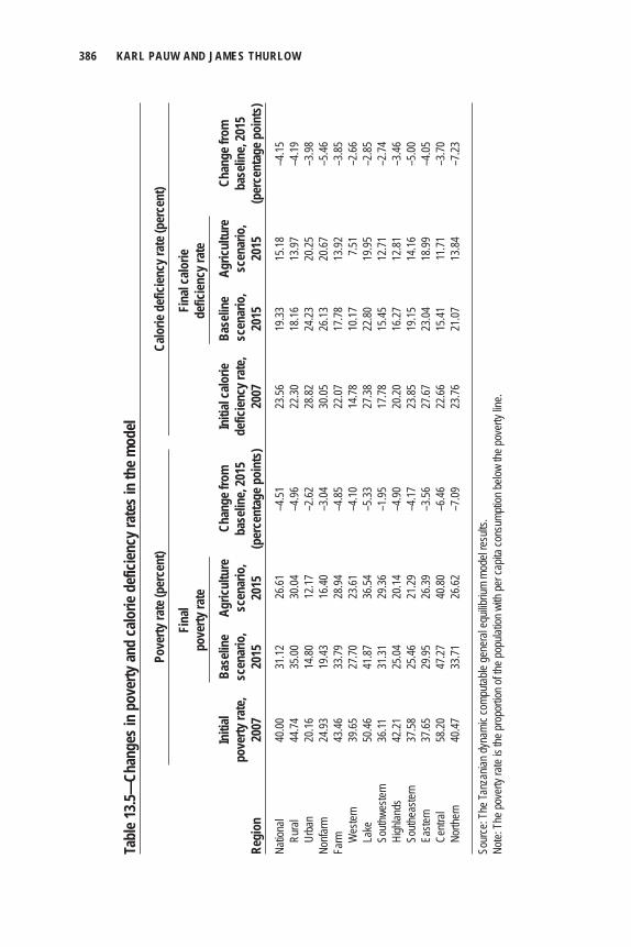
386 KARL PAUW AND JAMES THURLOW
Tabl
e 13.5
—Ch
ange
s in
pove
rty an
d ca
lorie
def
icien
cy ra
tes i
n th
e mod
el
Po
verty
rate
(per
cent
) Ca
lorie
def
icien
cy ra
te (p
erce
nt)
Fi
nal
Fina
l calo
rie
pove
rty ra
te
defic
iency
rate
In
itial
Base
line
Agric
ultu
re
Chan
ge fr
om
Initi
al ca
lorie
Ba
selin
e Ag
ricul
ture
Ch
ange
from
po
verty
rate
, sc
enar
io,
scen
ario
, ba
selin
e, 20
15
defic
iency
rate
, sc
enar
io,
scen
ario
, ba
selin
e, 20
15
Regi
on
2007
20
15
2015
(p
erce
ntag
e poi
nts)
20
07
2015
20
15
(per
cent
age p
oint
s)Na
tiona
l 40
.00
31.12
26
.61
–4.51
23
.56
19.33
15
.18
–4.15
Ru
ral
44.74
35
.00
30.04
–4
.96
22.30
18
.16
13.97
–4
.19
Urba
n 20
.16
14.80
12
.17
–2.62
28
.82
24.23
20
.25
–3.98
Nonfa
rm
24.93
19
.43
16.40
–3
.04
30.05
26
.13
20.67
–5
.46Fa
rm
43.46
33
.79
28.94
–4
.85
22.07
17
.78
13.92
–3
.85
Wes
tern
39.65
27
.70
23.61
–4
.10
14.78
10
.17
7.51
–2.66
La
ke
50.46
41
.87
36.54
–5
.33
27.38
22
.80
19.95
–2
.85
South
weste
rn
36.11
31
.31
29.36
–1
.95
17.78
15
.45
12.71
–2
.74
High
lands
42
.21
25.04
20
.14
–4.90
20
.20
16.27
12
.81
–3.46
So
uthea
stern
37
.58
25.46
21
.29
–4.17
23
.85
19.15
14
.16
–5.00
Ea
stern
37
.65
29.95
26
.39
–3.56
27
.67
23.04
18
.99
–4.05
Ce
ntral
58.20
47
.27
40.80
–6
.46
22.66
15
.41
11.71
–3
.70
North
ern
40.47
33
.71
26.62
–7
.09
23.76
21
.07
13.84
–7
.23
Sour
ce: T
he Ta
nzan
ian dy
nami
c com
putab
le ge
nera
l equ
ilibriu
m mo
del re
sults
. No
te: T
he po
verty
rate
is the
prop
ortio
n of th
e pop
ulatio
n with
per c
apita
cons
umpti
on be
low th
e pov
erty
line.
TANZANIA 387
from the household surveys for 2001–07. However, the model’s results are reason-ably consistent with the distributional changes observed for this period. There is also a 4.23 percentage point (or 2.44 percent) reduction in the calorie defi ciency rate during this period. This decline translates into a calorie–growth elasticity of 0.68 (2.44 divided by 3.59), which is within the 0.26–0.78 range observed during 2001–07.
The baseline scenario offers three insights into the current poverty–growth relationship in Tanzania. First, the level of agricultural GDP growth reported in national accounts is consistent with subsector-level production trends. Second, the distributional impact of the current growth path is consistent with the small change in inequality reported in the household surveys between 2001 and 2007 (that is, the model and surveys produce similar poverty–growth elasticities). These two fi nd-ings suggest that either the level of nonagricultural growth is overestimated in national accounts, or the rate of poverty reduction is underestimated in the house-hold surveys, or both. Third, the composition of economic growth, particularly agricultural growth, has large implications for the rate of poverty reduction. Rapid growth in traditional exports during 2000–07 mainly benefi ted farmers in the regions where these crops are grown. Similarly, the expansion of certain crops, such as sugarcane and wheat, was more likely to benefi t large-scale farmers, who, in turn, are less likely to be poor. In contrast, declining per capita maize production slowed down real per capita income growth for poor farmers throughout the country.
The unevenness of growth is evident in Table 13.4, which shows changes in regional agricultural GDP in the baseline scenario. Agricultural GDP growth is high-est in the Western, Northern, and Eastern zones, where the country produces most of its fast-growing sugarcane, tobacco, and cotton. Growth is slowest in the Southeastern zone, where farmers rely more heavily on slower-growing maize, cashews, and poultry. Thus, even though the overall level of agricultural GDP growth is high in Tanzania, its composition is such that it does not benefi t all farmers equally, and to some extent it excludes certain regions and many of the country’s poorer farm-ers. Tanzania must therefore accelerate economic growth in sectors with stronger links to poorer households and regions if it is to signifi cantly reduce poverty.
Accelerated Growth Scenarios
Raising Agricultural ProductionIn this section we use the DCGE model to accelerate agricultural growth in a wider range of subsectors than those that led the growth process during 2000–07. More specifi cally, in the Agriculture scenario we increase production in agriculture’s sub-sectors beyond what was achieved in the baseline scenario. Land expansion does not
388 KARL PAUW AND JAMES THURLOW
increase beyond its current 2 percent growth rate; instead, productivity growth in individual subsectors is increased (starting from 2010). Taking maize as an example, we increase the annual yield growth rate from 1.45 percent in the baseline scenario to 3.94 percent in the Agriculture scenario (see Table 13.3). Accordingly, while cur-rent trends predict maize yields will rise from 0.91 metric tons per hectare (mt/ha) to 1.10 mt/ha during 2009–15, in the Agriculture scenario they rise to 1.24 mt/ha. Thus, overall maize production increases by 1 million tons over 2009–15, which is twice what is expected based on current trends (see Table 13.3). In contrast, wheat and tobacco production do not grow much faster in the Agriculture scenario, because these crops have already expanded rapidly in the baseline scenario. This process of improving crop yields and increasing production is repeated for all agri-cultural subsectors.
Annual agricultural GDP growth rises from 3.97 percent in the baseline sce-nario to 5.87 percent in the Agriculture scenario during 2009–15 (see Table 13.4). Agricultural growth is now also more broadly based, with most crops growing more rapidly. The largest improvement is in horticulture, where the previous decline in vegetable yields is now reversed. The growth rate in export crops now averages almost 10 percent per year, suggesting that there is still considerable growth poten-tial in export agriculture. Average livestock GDP growth also rises by 1.5 percentage points. Faster agricultural growth generates strong forward-linkage effects for upstream food processing, which benefi ts from increased supply of maize and live-stock products for the grain milling and meat subsectors. There is, however, only a small increase in other agroprocessing, because tobacco refi ning was already growing rapidly in the baseline scenario. Overall, the expansion of agriculture and upstream sectors causes the growth rate of total national GDP to increase from 6.17 to 6.83 percent per year in the Agriculture scenario.
Agricultural growth is now more evenly distributed across regions. In the base-line scenario, agricultural growth was concentrated in rice, wheat, and certain tradi-tional export crops. In the Agriculture scenario all regions benefi t from broader-based growth. For example, the Southeast zone was the slowest growing region in the base-line scenario, with annual agricultural growth of only 2 percent. This rate now increases to more than 5 percent per year, driven by maize, cashews, and coconuts, which are important crops for this part of the country. However, regional inequality in agricultural growth still widens, because such areas as the Northern and Highlands zones benefi t from faster export crop growth, particularly for coffee, tea, and sisal, which are more likely to benefi t large-scale farmers (see Table 13.1).
Market Constraints and Price EffectsIncreasing agricultural production causes prices to fall if there are demand or market constraints. We expect prices to fall for commodities (1) whose production has
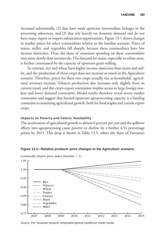
TANZANIA 389
increased substantially, (2) that have weak upstream intermediate linkages in the processing subsectors, and (3) that rely heavily on domestic demand and do not have many export or import substitution opportunities. Figure 13.1 shows changes in market prices for select commodities relative to the baseline scenario. Prices of maize, millet, and vegetables fall sharply, because these commodities have low income elasticities. Thus, the share of consumer spending on these commodities rises more slowly than incomes do. The demand for maize, especially in urban areas, is further constrained by the capacity of upstream grain milling.
In contrast, rice and wheat have higher income elasticities than maize and mil-let, and the production of these crops does not increase as much in the Agriculture scenario. Therefore, prices for these two crops actually rise as households’ agricul-tural revenues increase. Tobacco production also increases only slightly from its current trend, and this crop’s export orientation implies access to large foreign mar-kets and lower demand constraints. Model results therefore reveal severe market constraints and suggest that limited upstream agroprocessing capacity is a binding constraint to sustaining agricultural growth, both for food staples and certain export crops.
Impacts on Poverty and Caloric AvailabilityThe acceleration of agricultural growth to almost 6 percent per year and the spillover effects into agroprocessing cause poverty to decline by a further 4.51 percentage points by 2015. This drop is shown in Table 13.5, where the share of Tanzania’s
Commodity relative price index (baseline � 1)
1.05
0.7520152014
PoultryCassavaMaize
WheatTobaccoRice
0.95
1.00
0.90
0.85
0.80
2013201220112010200920082007
VegetablesMillet
Figure 13.1—Relative producer price changes in the Agriculture scenario
Source: The Tanzanian dynamic computable general equilibrium model results.
390 KARL PAUW AND JAMES THURLOW
population below the poverty line is 26.61 percent by 2015 in the Agriculture sce-nario compared to 31.12 percent in the baseline scenario. Thus, taking 2.5 percent annual population growth into account, achieving the productivity improvements in Table 13.3 lifts an additional 1.74 million people above the poverty line by 2015. The acceleration of broadly based agricultural growth also strengthens the poverty–growth relationship in Tanzania. For example, the additional 2 percent agricultural growth each year causes the poverty–growth elasticity to rise from 0.86 in the base-line scenario to 1.36 in the Agriculture scenario. This increase is a result of per capita GDP now growing at 4.33 percent per year during 2009–15 and the poverty rate declining by 5.89 percent per year (that is, 5.89 divided by 4.33). Because we only increase agricultural growth in the Agriculture scenario, the increase in the poverty–growth elasticity relative to the baseline scenario implies that broadly based agricul-tural growth is more pro-poor than nonagricultural growth is.
All household groups in the DCGE model benefi t from accelerated agricultural growth (see Table 13.5). Not surprisingly, the rural poverty rate declines substan-tially in the Agriculture scenario (by 4.96 percentage points). Poverty reduction is largest in the Northern and Central zones, where poor households benefi t from enhanced growth in millet and livestock, and to a lesser extent from out-grower export crops, such as coffee. Improved production of plantains, vegetables, and pulses also favors poor households in the Lake zone. In contrast, the drop in poverty is smaller in the Southwest zone, because these households rely more heavily on nonfarm incomes, and so their incomes are less affected by increased agricultural revenues. Finally, although urban and nonfarm households do not benefi t directly from agricultural revenues, they do benefi t from falling consumer prices. Even urban nonfarm households in the highest expenditure quintile spend about half of their incomes on purchased foods. More importantly, nonfarm households in the lower expenditure quintiles spend as much as three-quarters of their incomes on agricul-tural products. Forward consumption linkages therefore explain why the urban poverty rate falls by 2.62 percentage points in the Agriculture scenario.
Agricultural growth also benefi ts household caloric intake by increasing incomes and food availability in the country. As a result, the share of the national population consuming less than 2,550 kilocalories per day falls by 4.15 percentage points, which is over and above the 4.23 percentage point reduction already occurring in the base-line scenario (see Table 13.5). The initial calorie–growth elasticity was 0.68 in the baseline scenario, but model results now show that accelerating broadly based agri-cultural growth greatly enhances this growth–nutrition relationship, with the elastic-ity rising to 1.48 in the Agriculture scenario. This increase is driven primarily by increased production and consumption of calorie-rich maize, pulses, and millet.
The distribution of changes in nutritional outcomes differs from that of poverty outcomes. Most striking perhaps is the larger reduction in the calorie defi ciency rate
TANZANIA 391
for urban nonfarm households compared to rural households. Increased production and falling prices for key food staples greatly improve urban household nutritional status. Part of the reason for this larger decline is that urban households currently have higher calorie defi ciency rates than rural households. However, although all house-holds benefi t from increased maize availability, urban nonfarm households, com-pared to rural households, also derive a larger share of their calorie intake from pulses, vegetables, and livestock products. These crops grow particularly fast in the Agriculture scenario.
In summary, accelerating agricultural growth greatly strengthens both the poverty–growth and growth–nutrition relationships in Tanzania. These linkages are driven by the broader base of agricultural growth, which allows key calorie-laden foodcrops, such as maize and millet, to expand production. These crops are also more widespread in Tanzania than are export crops, implying greater participation of smallholder farmers in a larger number of regions in the country. Ultimately, the model results indicate that agricultural growth is substantially more pro-poor than nonagricultural growth, as evidenced by the large increase in the overall poverty–growth elasticity in the Agriculture scenario. At the same time it has the ability to improve nutritional outcomes because of the increased availability of food at lower prices across the spectrum of households.
Comparing Alternative Sources of Agricultural Growth We now compare alternative sources of growth in terms of their effectiveness in reducing poverty, improving household calorie availability, and stimulating overall economic growth in the country. Agricultural subsectors can have different impacts on development outcomes for a variety of reasons. First, certain subsectors are already large, and so small yield improvements can have large implications for agri-cultural and national economic growth. Second, smaller subsectors may have large growth potentials, so they can contribute to overall growth through their rapid expansion. Third, some sectors are more effective at reducing poverty, because they have stronger linkages to poor households’ income-generation process, or they pro-duce products that poor households consume intensively. Fourth, some subsectors produce products that are particularly important for household nutritional status, such as those that are cost-effective sources of calories and other minerals or are consumed intensively by nutrient-defi cient households. Finally, some agricultural subsectors have stronger linkages to upstream processing, so expanding production in these subsectors generates more growth outside of agriculture. We consider these fi ve criteria when prioritizing subsectors.
Table 13.6 presents poverty–growth elasticities for individual subsectors. Each subsector grows at a different rate in the Agriculture scenario. To produce compa-rable indicators, we normalize elasticities by assuming that all additional per capita
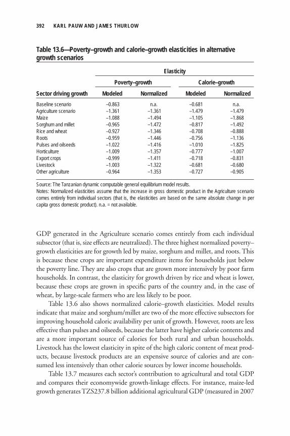
392 KARL PAUW AND JAMES THURLOW
GDP generated in the Agriculture scenario comes entirely from each individual subsector (that is, size effects are neutralized). The three highest normalized poverty–growth elasticities are for growth led by maize, sorghum and millet, and roots. This is because these crops are important expenditure items for households just below the poverty line. They are also crops that are grown more intensively by poor farm households. In contrast, the elasticity for growth driven by rice and wheat is lower, because these crops are grown in specifi c parts of the country and, in the case of wheat, by large-scale farmers who are less likely to be poor.
Table 13.6 also shows normalized calorie–growth elasticities. Model results indicate that maize and sorghum/millet are two of the more effective subsectors for improving household caloric availability per unit of growth. However, roots are less effective than pulses and oilseeds, because the latter have higher calorie contents and are a more important source of calories for both rural and urban households. Livestock has the lowest elasticity in spite of the high caloric content of meat prod-ucts, because livestock products are an expensive source of calories and are con-sumed less intensively than other calorie sources by lower income households.
Table 13.7 measures each sector’s contribution to agricultural and total GDP and compares their economywide growth-linkage effects. For instance, maize-led growth generates TZS237.8 billion additional agricultural GDP (measured in 2007
Table 13.6—Poverty–growth and calorie–growth elasticities in alternative growth scenarios
Elasticity
Poverty–growth Calorie–growth
Sector driving growth Modeled Normalized Modeled NormalizedBaseline scenario –0.863 n.a. –0.681 n.a.Agriculture scenario –1.361 –1.361 –1.479 –1.479Maize –1.088 –1.494 –1.105 –1.868Sorghum and millet –0.965 –1.472 –0.817 –1.492Rice and wheat –0.927 –1.346 –0.708 –0.888Roots –0.959 –1.446 –0.756 –1.136Pulses and oilseeds –1.022 –1.416 –1.010 –1.825Horticulture –1.009 –1.357 –0.777 –1.007Export crops –0.999 –1.411 –0.718 –0.831Livestock –1.003 –1.322 –0.681 –0.680Other agriculture –0.964 –1.353 –0.727 –0.905
Source: The Tanzanian dynamic computable general equilibrium model results.Notes: Normalized elasticities assume that the increase in gross domestic product in the Agriculture scenario comes entirely from individual sectors (that is, the elasticities are based on the same absolute change in per capita gross domestic product). n.a. = not available.
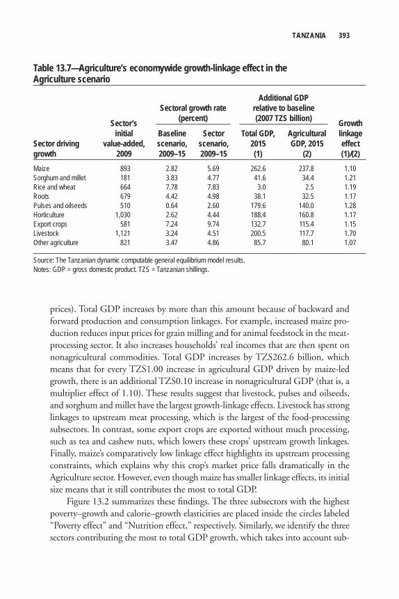
TANZANIA 393
prices). Total GDP increases by more than this amount because of backward and forward production and consumption linkages. For example, increased maize pro-duction reduces input prices for grain milling and for animal feedstock in the meat-processing sector. It also increases households’ real incomes that are then spent on nonagricultural commodities. Total GDP increases by TZS262.6 billion, which means that for every TZS1.00 increase in agricultural GDP driven by maize-led growth, there is an additional TZS0.10 increase in nonagricultural GDP (that is, a multiplier effect of 1.10). These results suggest that livestock, pulses and oilseeds, and sorghum and millet have the largest growth-linkage effects. Livestock has strong linkages to upstream meat processing, which is the largest of the food-processing subsectors. In contrast, some export crops are exported without much processing, such as tea and cashew nuts, which lowers these crops’ upstream growth linkages. Finally, maize’s comparatively low linkage effect highlights its upstream processing constraints, which explains why this crop’s market price falls dramatically in the Agriculture sector. However, even though maize has smaller linkage effects, its initial size means that it still contributes the most to total GDP.
Figure 13.2 summarizes these fi ndings. The three subsectors with the highest poverty–growth and calorie–growth elasticities are placed inside the circles labeled “Poverty effect” and “Nutrition effect,” respectively. Similarly, we identify the three sectors contributing the most to total GDP growth, which takes into account sub-
Table 13.7—Agriculture’s economywide growth-linkage effect in the Agriculture scenario
Sector’s Growth initial Baseline Sector Total GDP, Agricultural linkageSector driving value-added, scenario, scenario, 2015 GDP, 2015 effectgrowth 2009 2009–15 2009–15 (1) (2) (1)/(2)Maize 893 2.82 5.69 262.6 237.8 1.10Sorghum and millet 181 3.83 4.77 41.6 34.4 1.21Rice and wheat 664 7.78 7.83 3.0 2.5 1.19Roots 679 4.42 4.98 38.1 32.5 1.17Pulses and oilseeds 510 0.64 2.60 179.6 140.0 1.28Horticulture 1,030 2.62 4.44 188.4 160.8 1.17Export crops 581 7.24 9.74 132.7 115.4 1.15Livestock 1,121 3.24 4.51 200.5 117.7 1.70Other agriculture 821 3.47 4.86 85.7 80.1 1.07
Source: The Tanzanian dynamic computable general equilibrium model results.Notes: GDP = gross domestic product. TZS = Tanzanian shillings.
Sectoral growth rate (percent)
Additional GDPrelative to baseline(2007 TZS billion)
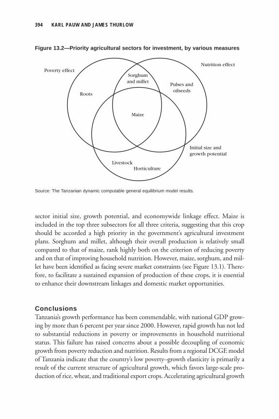
394 KARL PAUW AND JAMES THURLOW
sector initial size, growth potential, and economywide linkage effect. Maize is included in the top three subsectors for all three criteria, suggesting that this crop should be accorded a high priority in the government’s agricultural investment plans. Sorghum and millet, although their overall production is relatively small compared to that of maize, rank highly both on the criterion of reducing poverty and on that of improving household nutrition. However, maize, sorghum, and mil-let have been identifi ed as facing severe market constraints (see Figure 13.1). There-fore, to facilitate a sustained expansion of production of these crops, it is essential to enhance their downstream linkages and domestic market opportunities.
Conclusions Tanzania’s growth performance has been commendable, with national GDP grow-ing by more than 6 percent per year since 2000. However, rapid growth has not led to substantial reductions in poverty or improvements in household nutritional status. This failure has raised concerns about a possible decoupling of economic growth from poverty reduction and nutrition. Results from a regional DCGE model of Tanzania indicate that the country’s low poverty–growth elasticity is primarily a result of the current structure of agricultural growth, which favors large-scale pro-duction of rice, wheat, and traditional export crops. Accelerating agricultural growth
Poverty effectNutrition effect
Pulses andoilseeds
Maize
Sorghumand millet
Roots
Initial size andgrowth potential
LivestockHorticulture
Figure 13.2—Priority agricultural sectors for investment, by various measures
Source: The Tanzanian dynamic computable general equilibrium model results.
TANZANIA 395
in a wider range of subsectors than those currently leading the growth process is needed to strengthen the effectiveness of growth at reducing poverty and improving household nutritional status.
The modeling analysis described in this chapter did not explicitly consider how increased agricultural productivity might be achieved, or what the cost might be in terms of investments, extension services, or subsidies. Our discussion, however, pointed out how investment in agricultural research and development in Tanzania is likely to yield high returns. However, the Government of Tanzania has only spent a small share of its budget on agriculture in recent years. Additional spending on agriculture, particularly on research and development and extension, is therefore needed, along with improved effi ciency in the way the Ministry of Agriculture spends its budget allocation.
Model results identifi ed maize as a priority sector for investment. Already empirical evidence suggests that maize yields in Tanzania are rising thanks to the provision of extension services and farmers’ increased use of improved inputs, espe-cially fertilizer (Nkonya, Schroder, and Norman 1997). Investment in rural educa-tion is also found to encourage greater adoption of improved technologies. However, much of Tanzania’s maize production is rainfed, thus making the country highly susceptible to extreme climate events and high market price volatility. In this regard, evidence suggests that lowering transaction costs through investing in rural roads would reduce price volatility in Tanzania and also increase farmgate prices, thereby enhancing returns to maize farming (Kilima et al. 2008). Our model results also identifi ed severe market constraints facing maize production in Tanzania. Expanding upstream milling capacity would strengthen farmer access to urban consumers who demand more processed maize, thus relieving some of the downward pressure on maize prices. Similarly, model results also suggest that opportunities exist for domes-tic producers to substitute for imported cereals.
Finally, the model results provided two insights into the current inconsistencies between the rapid economic growth reported in national accounts and the small improvements in poverty and nutrition from the household surveys. First, estimates in national accounts of agricultural growth are found to be consistent with subsector-level production trends. Second, the model and surveys produced similar estimates of the poverty–growth elasticity, suggesting that the structure of growth is consistent with only small changes in inequality. These two fi ndings suggest that either the level of nonagricultural growth is overestimated in national accounts or the rate of poverty reduction is underestimated in the household surveys, or both. Regardless of these inconsistencies, however, the model results confi rm the weak relationships between economic growth, poverty reduction, and nutrition in Tanzania. They under-line the importance of encouraging broader-based economic growth in the future, with a stronger role for agriculture and foodcrops in particular.
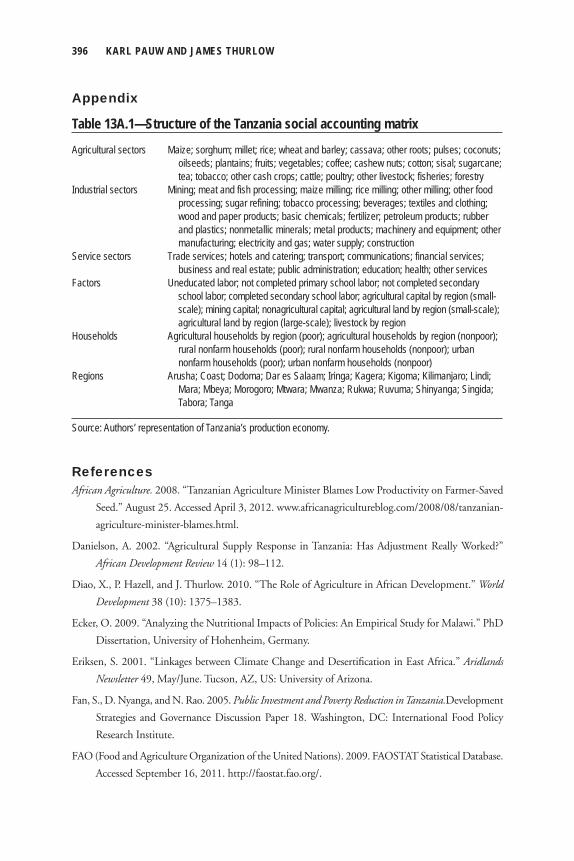
396 KARL PAUW AND JAMES THURLOW
Appendix
Table 13A.1—Structure of the Tanzania social accounting matrix
Agricultural sectors Maize; sorghum; millet; rice; wheat and barley; cassava; other roots; pulses; coconuts; oilseeds; plantains; fruits; vegetables; coffee; cashew nuts; cotton; sisal; sugarcane;
tea; tobacco; other cash crops; cattle; poultry; other livestock; fisheries; forestryIndustrial sectors Mining; meat and fish processing; maize milling; rice milling; other milling; other food processing; sugar refining; tobacco processing; beverages; textiles and clothing;
wood and paper products; basic chemicals; fertilizer; petroleum products; rubber and plastics; nonmetallic minerals; metal products; machinery and equipment; other manufacturing; electricity and gas; water supply; construction
Service sectors Trade services; hotels and catering; transport; communications; financial services; business and real estate; public administration; education; health; other servicesFactors Uneducated labor; not completed primary school labor; not completed secondary school labor; completed secondary school labor; agricultural capital by region (small-
scale); mining capital; nonagricultural capital; agricultural land by region (small-scale); agricultural land by region (large-scale); livestock by region
Households Agricultural households by region (poor); agricultural households by region (nonpoor); rural nonfarm households (poor); rural nonfarm households (nonpoor); urban
nonfarm households (poor); urban nonfarm households (nonpoor)Regions Arusha; Coast; Dodoma; Dar es Salaam; Iringa; Kagera; Kigoma; Kilimanjaro; Lindi; Mara; Mbeya; Morogoro; Mtwara; Mwanza; Rukwa; Ruvuma; Shinyanga; Singida;
Tabora; Tanga
Source: Authors’ representation of Tanzania’s production economy.
ReferencesAfrican Agriculture. 2008. “Tanzanian Agriculture Minister Blames Low Productivity on Farmer-Saved
Seed.” August 25. Accessed April 3, 2012. www.africanagricultureblog.com/2008/08/tanzanian-
agriculture-minister-blames.html.
Danielson, A. 2002. “Agricultural Supply Response in Tanzania: Has Adjustment Really Worked?”
African Development Review 14 (1): 98–112.
Diao, X., P. Hazell, and J. Thurlow. 2010. “The Role of Agriculture in African Development.” World
Development 38 (10): 1375–1383.
Ecker, O. 2009. “Analyzing the Nutritional Impacts of Policies: An Empirical Study for Malawi.” PhD
Dissertation, University of Hohenheim, Germany.
Eriksen, S. 2001. “Linkages between Climate Change and Desertifi cation in East Africa.” Aridlands
Newsletter 49, May/June. Tucson, AZ, US: University of Arizona.
Fan, S., D. Nyanga, and N. Rao. 2005. Public Investment and Poverty Reduction in Tanzania.Development
Strategies and Governance Discussion Paper 18. Washington, DC: International Food Policy
Research Institute.
FAO (Food and Agriculture Organization of the United Nations). 2009. FAOSTAT Statistical Database.
Accessed September 16, 2011. http://faostat.fao.org/.
TANZANIA 397
JGDPG (Joint Government and Development Partners Group). 2009. “Accelerating Pro-Poor Growth
in the Context of Kilimo Kwanza.” Paper presented at the Annual National Policy Dialogue, Dar
es Salaam, Tanzania, November 23. http://www.tzonline.org/pdf/kilimokwanza2009.pdf.
Kilima, F. T. M., C. Chung, P. Kenkel, and E. R. Mbiha. 2008. “Impact of Market Reform on Spatial
Volatility of Maize Prices in Tanzania.” Journal of Agricultural Economics 59 (2): 257–270.
Lukmanji, Z., E. Hertzmark, N. Mlingi, V. Assey, G. Ndossi, and W. Fawzi. 2008. Tanzania Food
Composition Tables. First Edition. Dar es Salaam, Tanzania; Dar es Salaam, Tanzania; Boston:
Muhimbili University of Health and Allied Sciences; Tanzania Food and Nutrition Centre;
Harvard School of Public Health.
Malley, Z. J. U., M. Taeb, and T. Matsumoto. 2009. “Agricultural Productivity and Environmental
Insecurity in the Usangu Plain, Tanzania: Policy Implications for Sustainability of Agriculture.”
Environment, Development and Sustainability 11: 175–195.
Meertens, B. 2000. “Agricultural Performance in Tanzania under Structural Adjustment Programs: Is
It Really So Positive?” Agriculture and Human Values 17 (4): 333–346.
Mellor, J. W. 1999. Faster, More Equitable Growth: The Relation between Growth in Agriculture and
Poverty Reduction. Cambridge, MA, US: Harvard University Press.
Mmbaga, T. E., and C. Y. Lyamchai. 2001. “Drought Management Options in Maize Production in
Northern Tanzania.” Paper presented at the 7th Eastern and Southern Africa Regional Maize
Conference, Nairobi, Kenya, February 11–15. http://apps.cimmyt.org/english/docs/proceedings/
africa/pdf/58_Mmbaga.pdf.
Morris, M., V. A. Kelly, R. J. Kopicki, and D. Byerlee. 2007. Fertilizer Use in African Agriculture. Lessons
Learned and Good Practice Guidelines. Washington, DC: World Bank.
Nkonya, E., T. Schroder, and D. Norman. 1997. “Factors Affecting Adoption of Improved Maize Seed
and Fertiliser in Northern Tanzania.” Journal of Agricultural Economics 48 (1–3): 1–12.
Putterman, L. 1995. “Economic Reform and Smallholder Agriculture in Tanzania: A Discussion of
Recent Market Liberalization, Road Rehabilitation, and Technology Dissemination Efforts.”
World Development 23 (2): 311–326.
Ravallion, M. 2001. Measuring Aggregate Welfare in Developing Countries: How Well Do National
Accounts and Survey Agree? Policy Research Working Paper 2665. Washington, DC: World
Bank.
Ravallion, M., and G. Datt. 1996. “How Important to India’s Poor Is the Sectoral Composition of
Economic Growth?” World Bank Economic Review 10 (1): 1–26.
Sanchez, P. A., G. L. Denning, and G. Nziguheba. 2009. “The African Green Revolution Moves
Forward.” Food Security 1: 37–44.
Tanzania, MAFSC (Ministry of Agriculture, Food Security, and Cooperatives). 2004. National Sample
Census of Agriculture, 2002/2003. Dar es Salaam, Tanzania.
———. 2006. Agriculture Basic Data 1998/99–2004/05. Dar es Salaam, Tanzania.
398 KARL PAUW AND JAMES THURLOW
Tanzania, MFEA (Ministry of Finance and Economic Affairs). 2008. The Economic Survey 2007. Dar
es Salaam, Tanzania.
Tanzania, NBI (National Bureau of Statistics). 2002. Household Budget Survey 2000/01. Dar es Salaam,
Tanzania.
Thirtle, C., Lin, L., and Piesse, J. 2003. “The Impact of Research-Led Agricultural Productivity Growth
on Poverty Reduction in Africa, Asia and Latin America.” World Development 31 (12):
1959–1975.
Thurlow, J., and P. Wobst. 2003. Poverty-Focused Social Accounting Matrices for Tanzania. Trade and
Macroeconomics Discussion Paper 112. Washington, DC: International Food Policy Research
Institute.
Timmer, C. P. 1988. “The Agricultural Transformation.” In Handbook of Development Economics.
Vol. 1, edited by H. Chenery and T. N. Srinivasan, 275–331. Amsterdam: North-Holland.
Treichel, V. 2005. Tanzania’s Growth Process and Success in Reducing Poverty. Working Paper 05/35.
Washington, DC: International Monetary Fund.
UNU, WHO, and FAO (United Nations University, World Health Organization, and Food and
Agriculture Organization of the United Nations). 2004. Human Energy Requirements: Report of a
Joint FAO/WHO/UNU Expert Consultation, Rome, October 17–24, 2001. FAO Food and Nutrition
Technical Report Series 1. Rome.
Wiig, H., J. B. Aune, S. Glomsrød, and V. Iversen. 2001. “Structural Adjustment and Soil Degradation
in Tanzania: A CGE Model Approach with Endogenous Soil Productivity.” Agricultural Economics
24 (3): 263–287.
Wolter, D. 2008. The Challenge of Moving from Subsistence to Profi t, Business for Development 2008.
Paris: OECD Development Centre, Organisation for Economic Cooperation and Development.
World Bank. 2007. Advancing Nutrition for Long-Term, Equitable Growth. Report 41315-TZ.
Washington, DC.
———. 2008. World Development Indicators. Washington, DC.
———. 2009. “Lost in Transition: Income Poverty Reduction since 2001.” Mimeo. Research and
Analysis Technical Working Group, World Bank, Dar es Salaam, Tanzania.
C h a p t e r 1 4
Lessons Learned and Remaining Challenges
Xinshen Diao and James Thurlow
The 2000s has been Africa’s “decade of growth.” For the first time since the 1970s, Africa has not been the slowest growing developing region in world. This was not necessarily because the rest of the world did badly—economic
growth in Africa was faster in the 2000s than in previous decades. This growth accel-eration was in spite of the food and financial crises, and subsequent global recession, which Africa appears to have weathered relatively well. Of course, economic growth is not the only measure of development, and the continent’s success in improving social indicators has been less impressive. Poverty and malnutrition remain severe and widespread, and the absolute number of poor people has continued to rise. Agriculture has also lagged behind national economic growth in most countries, thus further entrenching the rural–urban divide. In response to these conditions, many African governments have endorsed the Comprehensive Africa Agriculture Development Programme (CAADP), in which they commit to achieving at least 6 percent annual agricultural growth by allocating at least 10 percent of their national budgets to agricultural investments.
However, although governments may be assigning agriculture a more central role in national policy, opinions among researchers and development practitioners remain mixed. Agriculture’s proponents argue that Asia’s Green Revolution demon-strated the sector’s growth and transformative potential. In Africa, only agriculture is seen as having the size and economic linkages needed to generate broadly based, poverty-reducing growth—at least over a reasonable time horizon. In contrast, skeptics cite African agriculture’s poor past performance and the continent’s often unfavorable agroecological conditions. Moreover, globalization may have altered the
400 XINSHEN DIAO AND JAMES THURLOW
environment in which agriculture operates, and so the model of the Green Revolution may not be replicable in Africa today. The question of whether agricul-ture should be afforded a central role in African development is thus far from resolved.
A second area of the debate concerns whether staple foods or export-oriented crops should be the focus of African agricultural growth strategies. On the one hand, most poor smallholder farmers grow staple foods, and there is some scope for expanding regional food trade in Africa. Promoting staple foods could therefore directly benefi t the poor. On the other hand, traditional export crops normally have higher value and greater growth potential, and so their rapid growth might benefi t farmers more than slower-growing food staples. Export crops are also less dependent on domestic markets, which are underdeveloped in many African countries. Thus, even among agricultural proponents, there is still debate over what type of strategy is most appropriate for reducing poverty.
This book has provided new evidence for the debate and has demonstrated a method that can be used by governments to design more effective development strategies. Our recursive dynamic computable general equilibrium (DCGE) model is a semiempirical economywide framework calibrated to a country’s detailed eco-nomic structure. These features allow the model to capture both the macro- and microlevel dimensions of a country’s poverty–growth relationship. The 10 country case studies presented in this volume were drawn from low-income Africa to capture variation in (1) the size of the agricultural sector, (2) the extent of rural poverty, (3) agroecological conditions, (4) and geographic location. Together these case stud-ies represent the full diversity of low-income African countries.
The same approach was adopted in each country study. We fi rst developed a future baseline scenario based on observed trends from the past decade, and in so doing, estimated poverty changes under countries’ current growth trajectories. We then simulated accelerated growth in the whole agricultural sector and separately for individual agricultural subsectors. Subsector-level growth potentials were, in most cases, determined by research fi eld trials or in consultation with national agri-cultural ministries. The potential contribution of individual sectors to growth and poverty reduction was evaluated according to three criteria drawn from the on-going debate: (1) size and growth potential, (2) effectiveness in reducing poverty, and (3) ability to generate economywide growth. We also estimated the public re-sources needed to achieve faster agricultural growth. Here our methods ranged from integrated growth–investment analysis within the DCGE model (for example, Kenya), to top-down cost estimates (for example, Malawi) and detailed ex post itemized analysis (as in Rwanda).
In this fi nal chapter we consider the implications of the fi ndings from the case studies, fi rst, for the ongoing debate on the role of African agriculture and second,
LESSONS LEARNED AND REMAINING CHALLENGES 401
for the design of development strategies in Africa. We conclude by identifying areas where our methodology and analysis should be extended or improved.
Implications for the Debate on African Agriculture
Agricultural Growth Is Key to Achieving Pro-Poor Growth in AfricaResults from the case studies suggest that, in general, agriculture cannot be excluded from the current development model. As with Asia three decades ago, agriculture remains instrumental for future development in Africa. In terms of its contribution to economic growth, African agriculture has considerable potential, as demonstrated by the wide gaps between current productivity levels and those observed in agricultural research trials. The case studies showed how even fairly modest improvements in cur-rently low yields can greatly accelerate agricultural growth. Moreover, because agricul-ture generates between 20 and 50 percent of gross domestic product (GDP) in low-income African countries, faster agricultural growth will foster additional growth at the national level, including in nonagriculture. Thus, assigning a more active role to agriculture in Africa’s development process is justifi ed from a growth perspective.
Any effort to substantially reduce poverty in Africa will have to incorporate at least some role for agriculture. The scale of the rural poverty problem and the dependence of smallholders on agricultural incomes imply that investing in agricul-tural productivity is one the most effective policy instruments available. Not only does African agriculture have growth potential, but growth in the sector is also better at reducing poverty than is growth in nonagriculture. Table 14.1 summarizes the poverty–growth elasticities estimated in the case studies—specifi cally, those compar-ing agricultural growth to either nonagricultural growth or broadly based growth (that is, the baseline). Note that differences in how national poverty lines are defi ned prevents cross-country comparisons in the table.
In Kenya and Rwanda, for example, it was found that 1 percent national GDP growth driven by agriculture leads to three to four times more poverty reduction than does growth driven by nonagriculture. In other words, Kenyan industry would have to grow four times faster than agriculture to generate the same amount of poverty reduction at the national level. Two conclusions emerge from this observa-tion. First, although nonagriculture is obviously crucial for economic transforma-tion in Africa, the industrial sector may not provide a suffi cient platform for broadly based development unless it is linked to agriculture. Second, the weaker perfor-mance of African agriculture may explain why the continent’s “decade of growth” has not translated into a similarly impressive “decade of poverty reduction.”
The fi ndings from the case studies indicate that, throughout Africa, agricultural development is crucial for both economic growth and poverty reduction. However,
402 XINSHEN DIAO AND JAMES THURLOW
the results of our investment analyses showed that a great deal more public resources would be required to generate faster agricultural growth. Although empirical evi-dence suggests that there are positive returns to investing in agriculture (see, for example, the studies of Rwanda, Tanzania, and Uganda—Chapters 7, 13, and 10, respectively), the public sector cost of generating agricultural growth was not directly compared to that of nonagricultural growth. Thus, from a public policy perspective, comparable cost assessments are needed for nonagriculture if policymakers are to conclude that agriculture is the least expensive policy option for achieving growth and poverty-reduction targets. However, our fi ndings suggest that the returns to nonagricultural growth (in terms of total GDP generated) would need to be con-siderably higher than those obtained from agriculture to surpass the latter’s greater effectiveness in reducing poverty. Thus, despite the demands it places of public resources, agriculture may still be a more cost-effective policy option than nonagriculture.
Food Staples Should Be Afforded High Priority Export crops typically have higher value and growth potential than foodcrops, and so they provide a viable opportunity to raise rural households’ incomes. Indeed, the case studies showed how faster growth in export agriculture reduces rural poverty. However, the case studies also found that food staples are usually more effective than export agriculture at generating economywide growth and reducing poverty at the national level.
Table 14.1—Comparing the impact on poverty of agricultural and nonagricultural growth (percent)
Decline in national poverty rate resulting from a 1 percent increase in total gross domestic product
Country Baseline growth Agriculture-led growth Nonagriculture-led growthEthiopia –1.13 –1.41 –1.05Ghana –1.82 –1.95 n.a.Kenya –0.38 –2.20 –0.51Nigeria –0.85 –1.14 –0.73Rwanda –0.97 –1.53 –0.49Tanzania –0.86 –1.36 n.a.Uganda –0.80 –1.70 n.a.
Source: Authors, based on results reported in the country case studies.Notes: The poverty rate is the proportion of the population with per capita consumption below the poverty line. Differences in the definitions of national poverty lines mean that comparisons can be made across sectors but not countries. The Rwandan result in the baseline column is for the all-sectors scenario. Nonagriculture-led growth is industry only. n.a. = not available because the nonagricultural growth simulation was not run for this country (Malawi, Mozambique, and Zambia are omitted because no baseline elasticity was reported).
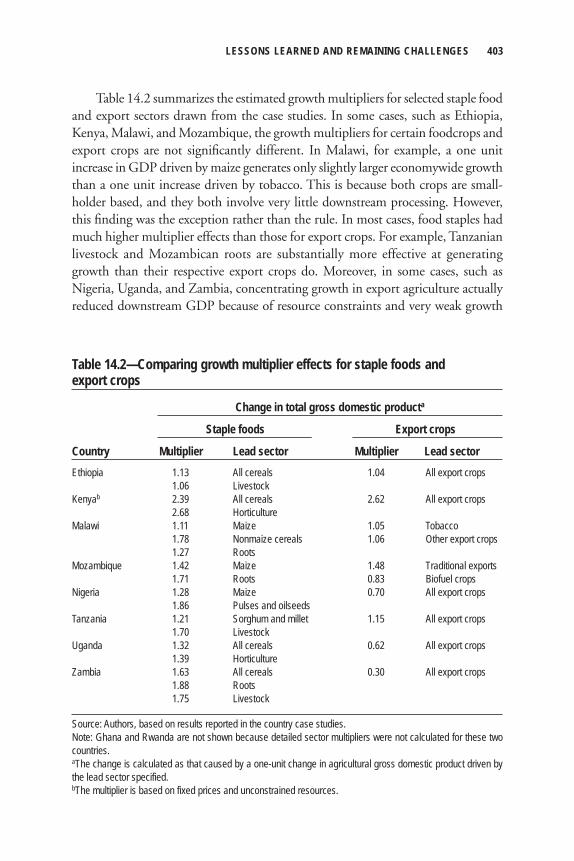
LESSONS LEARNED AND REMAINING CHALLENGES 403
Table 14.2 summarizes the estimated growth multipliers for selected staple food and export sectors drawn from the case studies. In some cases, such as Ethiopia, Kenya, Malawi, and Mozambique, the growth multipliers for certain foodcrops and export crops are not signifi cantly different. In Malawi, for example, a one unit increase in GDP driven by maize generates only slightly larger economywide growth than a one unit increase driven by tobacco. This is because both crops are small-holder based, and they both involve very little downstream processing. However, this fi nding was the exception rather than the rule. In most cases, food staples had much higher multiplier effects than those for export crops. For example, Tanzanian livestock and Mozambican roots are substantially more effective at generating growth than their respective export crops do. Moreover, in some cases, such as Nigeria, Uganda, and Zambia, concentrating growth in export agriculture actually reduced downstream GDP because of resource constraints and very weak growth
Table 14.2—Comparing growth multiplier effects for staple foods and export crops
Change in total gross domestic producta
Staple foods Export crops
Country Multiplier Lead sector Multiplier Lead sectorEthiopia 1.13 All cereals 1.04 All export crops 1.06 Livestock Kenyab 2.39 All cereals 2.62 All export crops 2.68 Horticulture Malawi 1.11 Maize 1.05 Tobacco 1.78 Nonmaize cereals 1.06 Other export crops 1.27 Roots Mozambique 1.42 Maize 1.48 Traditional exports 1.71 Roots 0.83 Biofuel cropsNigeria 1.28 Maize 0.70 All export crops 1.86 Pulses and oilseeds Tanzania 1.21 Sorghum and millet 1.15 All export crops 1.70 Livestock Uganda 1.32 All cereals 0.62 All export crops 1.39 Horticulture Zambia 1.63 All cereals 0.30 All export crops 1.88 Roots 1.75 Livestock
Source: Authors, based on results reported in the country case studies.Note: Ghana and Rwanda are not shown because detailed sector multipliers were not calculated for these two countries.aThe change is calculated as that caused by a one-unit change in agricultural gross domestic product driven by the lead sector specified. bThe multiplier is based on fixed prices and unconstrained resources.
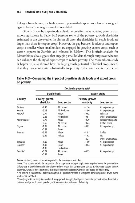
404 XINSHEN DIAO AND JAMES THURLOW
linkages. In such cases, the higher growth potential of export crops has to be weighed against losses in nonagricultural value-added.
Growth driven by staple foods is also far more effective at reducing poverty than export agriculture is. Table 14.3 presents some of the poverty–growth elasticities estimated in the case studies. In almost all cases, the elasticities for staple foods are larger than those for export crops. However, the gap between foodcrops and export crops is smaller when smallholders are engaged in growing export crops, such as cotton exports in Zambia and tobacco in Malawi. The biofuels analysis for Mozambique also suggests that engaging smallholders through outgrower schemes can enhance the ability of export crops to reduce poverty. The Mozambican study (Chapter 12) also showed how the large growth potential of biofuel crops means that they can contribute substantially to poverty reduction, despite their small
Table 14.3—Comparing the impact of growth in staple foods and export crops on poverty
Decline in poverty ratea
Staple foods Export crops
Country Poverty–growth Poverty–growth elasticity Lead sector elasticity Lead sectorEthiopia –1.40 All cereals –1.16 All export cropsKenya –2.13 All foodcrops –1.90 All export cropsMalawib –0.74 Maize –0.62 Tobacco –0.85 Horticulture –0.57 Other export cropsMozambiqueb –0.73 Maize –0.29 Traditional exports –0.65 All cereals –0.43 Biofuel cropsNigeria –1.02 All cereals –0.81 All export crops –0.92 Roots Rwanda –2.39 Maize –1.81 Coffee –2.59 Pulses –1.63 Tea –2.27 Other export cropsTanzania –1.09 Maize –1.00 All export cropsUgandab –1.07 Roots –0.64 All export crops –1.38 Horticulture Zambiab –0.27 All cereals –0.25 All export crops –0.33 Roots
Source: Authors, based on results reported in the country case studies.Notes: The poverty rate is the proportion of the population with per capita consumption below the poverty line. Differences in the definition of national poverty lines mean that comparisons can be made across sectors but not countries. Ghana is not shown because detailed sector elasticities were not calculated for this country.aThe decline is calculated as that resulting from a 1 percent increase in total gross domestic product driven by the lead sector specified.bPoverty–growth elasticity is calculated using growth in agricultural gross domestic product rather than that in national total gross domestic product, which reduces the estimates of elasticity.
LESSONS LEARNED AND REMAINING CHALLENGES 405
poverty–growth elasticity. However, in some countries, export agriculture would have to grow much faster than staple foods to achieve the same amount of poverty reduction. In Uganda, for example, growth driven by higher value horticulture is more than twice as effective at reducing poverty than is export-driven growth.
Our fi ndings address two aspects of the current debate on the role of agriculture in African development. First, we conclude that agriculture is still an essential ingre-dient in efforts to substantially raise economic growth and reduce poverty in Africa. A development strategy that attempts to bypass agriculture is unlikely to generate broadly based development. This conclusion supports African governments’ endorsement of the CAADP initiative. Second, within agriculture, staple foods are essential to generating pro-poor growth, although smallholder-based export agricul-ture can also contribute. Although we have painted the debate in stark contrasts, in reality it is a matter of emphasis. Our fi ndings suggest that supporting agriculture will be essential if the next 10 years are to be Africa’s decade of both growth and poverty reduction. The next section describes some of the broad insights that our case studies provide for the design of agricultural development strategies in Africa.
Lessons for African Development Strategies
Broadly Based Growth Is CrucialAlthough agriculture is an essential ingredient for African development, the contri-bution of nonagriculture should not be discounted. First, the fi ndings of the case studies confi rm the historical evidence from Asia and elsewhere: African countries must place suffi cient emphasis and resources on accelerating agricultural growth when preparing their development strategies. More specifi cally, the case studies indicate that faster agricultural growth is needed to reduce poverty and hunger at the national level, and hence, achieve the CAADP growth goal and the fi rst Millennium Development Goal for poverty reduction over a reasonable time frame (10–15 years).
The heterogeneous agroecological conditions in Africa are refl ected in highly diversifi ed production and consumption patterns. However, despite this diversity, agriculture remains a key development sector in all the low-income African case studies. In Kenya, for example, the analysis (Chapter 4) found that it is unlikely that a signifi cant decline in poverty can be achieved in the absence of agricultural growth, and so an industry-focused strategy that does not also invest in agriculture will exacerbate the country’s already high inequality. Similarly, the Ghanaian case study (Chapter 6) showed that a Green Revolution type of development is pro-poor and has economywide benefi ts through strong linkages between agriculture and the rest of the economy. In each country we found that not only do incomes of both rural

406 XINSHEN DIAO AND JAMES THURLOW
and urban households increase as a result of an agriculture-led growth strategy but also that the resulting additional demand for agricultural products can be met by domestic supply without signifi cantly lowering product prices. Agricultural growth favors broadly based development.
We also found that agricultural growth itself needs to be broadly based: it should involve multiple subsectors and also include the development of downstream nonagricultural sectors. A broadly based agricultural strategy emphasizes diversifi ed opportunities for a majority of farmers. This includes farmers in different locations, who face different agroecological conditions and have different farming technologies and systems. Most of our case studies found it unlikely that growth from a single agricultural subsector could generate enough economic growth on its own to sig-nifi cantly reduce national poverty. We also found that accelerating agricultural growth, even to 6 percent per year, is insuffi cient for most of the case-study countries to achieve the fi rst Millennium Development Goal. Faster nonagricultural growth and urban development are also needed.
Trying to achieve broadly based agricultural development will challenge govern-ments’ efforts to prioritize public investment across sectors and geographic locations. Growth in any country always occurs unevenly across subsectors and subnational regions. So even under a broadly based strategy, it is necessary to set priorities and sequence public investments and other interventions to support growth.
The Composition of Agricultural Growth MattersIndividual agricultural subsectors play different roles and have a diverse set of impacts on development outcomes. More specifi cally, an agricultural strategy is composed of a series of growth targets at the agricultural subsector level that should realistically take into account both the initial conditions and growth potential of these subsectors. Although agricultural potential is an important condition, it is not enough to determine targets. Furthermore, given new challenges, such as climate change and globalization, agricultural growth has to be driven by productivity improvements, even in relatively land-abundant countries. The following sugges-tions can be drawn for how to prioritize productivity-led agricultural growth at the subsector level.
First, the pro-poorness of an agricultural subsector’s growth should be at the top of the agenda in an agricultural strategy. Although agricultural growth is gener-ally pro-poor, different types of agricultural growth can lift a varying number of people out of poverty. The relationship between growth among different types of agricul-ture and poverty reduction depends on a country’s poverty distribution and sources of income among households. The pro-poorness of an agricultural subsector is also determined by who can participate in and benefi t from the growth of this sector and whether the sector has strong linkages and spillover effects to other economic activi-
LESSONS LEARNED AND REMAINING CHALLENGES 407
ties. Paying attention to the relationship between subsector agricultural growth and poverty reduction is an important step to ensuring that agricultural growth is pro-poor.
Second, policymakers setting priorities need to consider how subsectors are linked to the rest of the economy. A subsector with strong economywide linkages generates more gains for the economy as a whole than does a subsector with weak linkages. Spillover effects can be separated into production and consumption link-ages. Our case studies confi rm the importance of both types of linkages from agri-culture. However, export agriculture typically has less downstream value-addition, because products are often exported as raw materials. Promoting export agriculture may make it diffi cult for the country to develop labor-intensive manufacturing and services. So strategies should take advantage of new agricultural opportunities where they exist. Finding ways to strengthen domestic downstream processing is crucial if export crops are to provide a meaningful platform for rural and national development.
Third, targeting a relatively large agricultural sector for growth is essential if agriculture is to serve as an engine of economywide growth. Even though rapid growth can easily be achieved for a small subsector targeting niche markets (for example, growth in export-oriented horticultural products), the economywide impact of this subsector is small. The Nigerian case study (Chapter 8) shows that even with double-digit growth in a small subsector (for example, wheat or sugar), the overall growth could be insignifi cant. In contrast, a large agricultural subsector (such as rice or cassava) can create more growth in the whole economy, so that such sectors can become the leading force in the growth process. The Zambian case study (Chapter 11) found that although growth driven by either cereals or roots has con-siderable impact on poverty reduction, the small initial size and geographic concen-tration of certain foodcrops means that their potential contribution to national level growth and poverty reduction is limited, at least over the short term.
Fourth, the market opportunities of a subsector must be considered when set-ting priorities. Growth is not only determined by the productiveness of targeted agricultural subsectors but also by market access opportunities and conditions. Negative price effects are often an indicator of weak market opportunities or other constraints on market access. Domestic and export market opportunities (and import-substitution opportunities) are determined by the development of agro-processing industries, domestic and international trade policies, and market-access conditions (for example, regulations and information fl ows). For example, the Ugandan case study (Chapter 10) found that although cereals, roots, and matoke (plantains) are large sectors with high growth potentials, they face considerable market constraints, leading to large price declines when production increases. Thus, it is necessary to improve market conditions to realize the growth and poverty-
408 XINSHEN DIAO AND JAMES THURLOW
reducing potentials of prioritized crops. These improvements involve reducing transaction costs, supporting market development, and expanding downstream agroprocessing. One of the keys for successfully implementing agricultural strate-gies is therefore providing support interventions in sectors that are, strictly speak-ing, outside agriculture, such as rural road infrastructure and local and regional markets.
Both the Level and Efficiency of Public Agricultural Spending Needs to ImproveIncreasing agricultural growth will require additional investment in the sector as well as improvements in the effi ciency of public spending. Evidence from previous stud-ies has shown that public investment in agriculture and rural areas is a major deter-minant of agricultural growth and poverty reduction. Similarly, the country case studies in this volume indicate that, although there is huge potential in most coun-tries for agricultural growth and poverty reduction by closing yield gaps and increas-ing the effi ciency of available land use, realizing these goals will require substantial increases in agricultural investments. These investments include supporting rural roads, irrigation, education, extension, and research and development.
The case-study countries showed that, in most cases, what governments cur-rently spend on agriculture is not in accordance with agriculture’s important con-tribution to economic growth and poverty reduction. Moreover, our investment analyses revealed the need for increased agricultural and rural spending in almost all countries studied. The share of agricultural spending in total government expendi-ture would have to increase signifi cantly from current levels to meet countries’ stated growth and poverty-reduction targets. For example, the investment analysis in Uganda indicated that government spending on agriculture should grow by 25–30 percent per year to achieve and sustain CAADP’s 6 percent growth target. Over time the share of agriculture in the total economy and its importance in generating incomes will inevitably decline. But weak government support to agriculture or an early withdrawal of such support (or both) has been associated with a slowdown in economic transformation. This slowdown would create persistent inequalities and in the long run exacerbate the development challenge.
Achieving the stated development targets not only faces resource mobilization constraints but also is confronted with the challenge of allocating resources more effectively and effi ciently. A lack of effi ciency in public spending is a huge challenge in all case-study countries, and it exists for both agricultural and nonagricultural spending. Because public resources are scarce and opportunity costs high, public institutions need to be reformed, particularly those with any agriculture-related functions, to improve the provision and delivery of agricultural public goods and services. Although increased spending on agriculture is needed, the fi scal burden of
LESSONS LEARNED AND REMAINING CHALLENGES 409
an agricultural growth strategy can be reduced through improved effi ciency in fi scal management and implementation. More specifi cally, the case studies have found that improvements in the effi ciency of spending and providing agricultural services are one of the most important factors determining whether the country can achieve its agricultural growth and poverty-reduction goals. For example, improvements in the effi ciency of agricultural investments in Uganda meant that the government needed to allocate 6 percent less of its total budgetary resources to agriculture to achieve and sustain the targeted 6 percent agricultural growth. Thus, the ineffi ciency of public spending presents both a challenge and an opportunity to achieve future development at a manageable cost to the state.
Agricultural Strategies Need to Be Regionally DisaggregatedFinally, the heterogeneity of natural resources and economic environments in many developing countries necessitates regionally differentiated agricultural strategies. Many of our case studies showed that a single rapid agricultural growth strategy at the national level is insuffi cient to decrease regional inequalities and reduce poverty in lagging regions signifi cantly. In fact, similar rates of agricultural subsector growth at the subnational level were found to have different effects on associated poverty rates. For instance, poverty reduction in Tanzania is largest in the northern and central parts of the country, where poorer households benefi t from enhanced growth in millet and livestock and to a lesser extent from outgrower export crops, such as coffee. In contrast, the drop in poverty is smaller in regions where households rely more heavily on nonfarm incomes, so their incomes are less affected by increased agricultural revenues (Chapter 13). Similarly, the Kenyan case study (Chapter 4) showed that different interventions are needed to balance growth, poverty reduc-tion, and regional equity concerns.
The varying importance of crops and interventions in different parts of a coun-try highlights the need to design development strategies at the subnational level. This means taking into account how sectoral priorities vary across regions in a country and how they interact and contribute to national development objectives. The policies and interventions planned as part of an agricultural development strategy should therefore be combined with interventions specifi cally targeting lag-ging regions and population groups.
Extending the Methodology and Analysis Designing development strategies requires evidence that identifi es which policies and investments are most effective at achieving different (and often confl icting) development objectives. In this book we developed a DCGE modeling framework to evaluate alternative strategies in terms of economic growth and income poverty
410 XINSHEN DIAO AND JAMES THURLOW
reduction. Although our model provides useful insights to guide policy, it is cer-tainly not a panacea for all policy advice. Recognizing this limitation, we conclude by identifying fi ve areas where the modeling approach should be extended.
Integrating Investment AnalysisThe Kenyan case study (Chapter 4) fully integrated the DCGE modeling and investment analysis. This approach should be adopted in future studies, because ideally the growth–investment–poverty relationship should be modeled in a single consistent framework. To do this requires a multimethod approach based on econo-metrically estimated returns to public investments. The DCGE model then trans-lates these investments into changes in growth and poverty outcomes. There are a number of challenges to combining these two approaches.
First, the detailed investment data needed for the econometric analysis often do not exist at the country level, which is why we adopted a simpler cross-country approach (see Chapter 3). The temptation is to draw elasticities from other coun-tries, but this practice can create false precision. Transparency of assumptions might be more desirable than complex model integration, and the former may be better achieved by separating the growth–investment and poverty–growth components of the analysis (as was done in the Rwandan study in Chapter 7). Compiling country-level databases of public spending on different kinds of investment items (for example, research and development, extension, and irrigation) is therefore a pre-requisite for model integration.
Second, econometrics usually estimates net aggregate impacts without identify-ing specifi c impact pathways linking investments and outcomes. For example, econometric results may indicate a positive relationship between agricultural pro-ductivity and irrigation investments, but they do not identify which agricultural subsectors or regions are affected. The structural nature of DCGE models means that detailed pathways have to be explicitly defi ned. In some cases these pathways can be reasonably assumed or identifi ed by design. For example, investments in Zambian irrigation most likely target dry-season wheat farming or horticultural crops near urban areas. So irrigation investments in the model can be specifi ed so that they only benefi t these crops and regions. However, more complex interven-tions, such as agricultural research and development and extension, will inevitably require more challenging assumptions. Higher resolution microlevel analysis is therefore required, possibly using data from project-level monitoring and evaluation studies.
Finally, econometric studies rarely consider diminishing returns to public investments. They produce point estimates for elasticities based on historical levels and compositions of public spending. Understanding how investments interact with each other is crucial for DCGE models, whose economywide simulations normally
LESSONS LEARNED AND REMAINING CHALLENGES 411
involve reasonably large changes in specifi c investment levels. For example, Fan and Zhang (2008) fi nd that research and development and extension have higher returns than does education spending in rural Uganda. However, there may be some complementarity between education and extension or diminishing returns on exten-sion investment. Thus, a simulation that doubles investment in the extension system while assuming constant returns may be unfairly biased against other investment types. Much more detailed microlevel analysis is needed to appropriately calibrate a fully integrated public investment analysis in the DCGE model.
Modeling Farm and Household BehaviorAs mentioned in Chapter 2, although DCGE models capture both macro- and microlevel dimensions of the economy, their treatment of either dimension is less detailed than would be captured in more specialized partial equilibrium models. The chapters on Malawi, Uganda, and Zambia (Chapters 9, 10, and 11, respec-tively) incorporated some of the elements of representative farm models within the DCGE framework. Households were linked to their own specifi c production activi-ties and decided how best to allocate their land endowment across crop and livestock sectors. Greater integration of farm and DCGE models may provide a better repre-sentation of the constraints and opportunities facing smallholders and thus provide new policy insights. This modeling is distinct from occupational choice micro-simulation modeling, which focuses on how labor is allocated across households. This approach is less relevant for smallholder agriculture, where the primary deci-sion concerns land rather than labor allocations. Combining farm and DCGE models is technically challenging and, to our knowledge, has not been achieved in larger-scale semiempirical DCGE models.
Capturing Distributional EffectsThe case studies in this book focused on income or monetary poverty, that is, the proportion of the population in a country or region whose per capita consumption levels fall below a critical threshold or poverty line. Although commonly used, there are limitations to this approach.
The poverty headcount ratio is not only sensitive to the choice of poverty line, but it also attaches greater weight to households immediately above and below the poverty threshold. As a result, the full distributional effects of policies are poorly understood at the household level. More analysis is needed on how policies directly affect individuals and households. The sizable variance around the “typical” out-comes on poverty highlights the need to look beyond aggregate poverty impacts of specifi c growth options by focusing on the diversity of impacts underlying the aver-ages (Ravallion 2001). This point was demonstrated in the Kenyan case study (Chapter 4), where the growth incidence curves for growth driven by agriculture
412 XINSHEN DIAO AND JAMES THURLOW
and nonagriculture were strongly downward and upward sloping, respectively. Empirical evidence also shows that higher income households tend to capture a larger share of the increase in national incomes from growth than do lower income households (see, for example, Dollar and Kraay 2002). For example, an analysis of the distribution of income gains in China during 1990-1999 reveals wide diver-gence between rich and poor (Ravallion and Chen 2001).
Theory and evidence from developing countries indicates that the relationship between growth and income distribution is two sided (Bourguignon 2004). On the one hand, disparities in relative income play a central role in determining the rate and pattern of growth. On the other hand, country-level case studies fi nd that economic growth affects the distribution of income through a number of diverse channels, including institutional change, the segmentation of the economy, and changes in prices and factor returns. The exact channels through which distribu-tional change occurs depend heavily on initial conditions, with the pace and struc-ture of growth determining the relative importance of these channels. Accordingly, studies on development-policy choices should include the diverse distributional consequences of growth on poverty. Rather than treating poverty as a binary con-cept, as was done in most of the case studies in this volume, it is better to analyze outcomes across different income groups.
Looking beyond IncomeFuture research should give greater weight to measures that more accurately cap-ture the multidimensional aspects of poverty. Although no universally accepted defi nition of poverty exists, one of the most common descriptions of poverty is that it is a pronounced deprivation in well-being (World Bank 2001). Poverty is a multi-dimensional and complex phenomenon that goes beyond the one-dimensional monetary measures (such as income and consumption) of well-being and deprivation that are employed in nearly all empirical studies (Grosse, Harttgen, and Klasen 2008).
The Tanzanian case study (Chapter 13) extended the poverty analysis of other chapters to include an assessment of nutritional outcomes. It was found that sectors most effective at reducing poverty are not the same as those best at improving household nutritional status. Such differences confi rm the need for analyses of pro-poor growth to encompass a more comprehensive conceptualization of well-being and deprivation, including both economic and social factors. Various modeling approaches have included social outcome indicators (see, for example, Lofgren and Diaz-Bonilla 2010). However, these approaches face similar constraints to the inte-grated investment analysis described above: fi nding country-specifi c elasticities and identifying appropriate impact pathways can be diffi cult. To overcome this problem, there is also scope to link DCGE models top-down with sector models, such as
LESSONS LEARNED AND REMAINING CHALLENGES 413
demographic health and education system models, as was done in the Tanzania nutrition module.
Incorporating Risk and Social Protection Finally, the integration of risk and social protection policies with growth strategies is needed to advance pro-poor economic and social agendas concurrently. African farmers and governments face considerable uncertainty in their decisionmaking. Variables range from movements in world market prices to climate variability and extreme weather events, such as droughts and fl oods. Incorporating risk into the evaluation of different investments is essential for designing robust development strategies. Social protection is a key element of such analysis, because it encompasses public and private support systems that seek to prevent, mitigate, and manage risk, vulnerability, and chronic poverty among segments of the population. Although the building blocks of social protection interventions vary across countries, common instruments can take the form of social insurance (for example, health and property insurance), social assistance (for example, conditional and unconditional cash and food transfers), and services (such as child and adult education).
The connection between social protection and broader development is strong: social protection policies play an important role in supporting pro-poor growth. More specifi cally, risk and vulnerability act as a major impediment to human and economic development. The lack of effective social protection mechanisms obstructs the potential contribution of the poor to the development process, with, for exam-ple, the poorest people often developing less optimal survival strategies that perpetu-ate poverty, such as choosing low-productivity activities to reduce risk. Therefore, to maximize the poverty reduction and growth potential of specifi c development strategies, analyses of growth options need to factor in the potential impact of social protection policies. Rather than facing a trade-off between social protection and growth objectives, the synchronized pursuit of both interventions has the potential for complementarity, resulting in a virtuous cycle of equitable and pro-poor growth.
ReferencesBourguignon, F. 2004. The Poverty–Growth–Inequality Triangle. Working Paper 125. New Delhi, India:
Indian Council for Research on International Economic Relations.
Dollar, D., and A. Kraay. 2002. “Growth Is Good for the Poor.” Journal of Economic Growth 7 (3):
195–225.
Fan, S., and X. Zhang. 2008. “Public Expenditure, Growth, and Poverty Reduction in Rural Uganda.”
African Development Review 20 (3): 466–496.
Grosse, M., K. Harttgen, and S. Klasen. 2008. “Measuring Pro-Poor Growth in Non-Income
Dimensions.” World Development 36 (6): 1021–1047.

414 XINSHEN DIAO AND JAMES THURLOW
Lofgren, H., and C. Diaz-Bonilla. 2010. MAMS: An Economywide Model for Development Strategy
Analysis. Washington, DC: World Bank.
Ravallion, M. 2001. “Growth, Inequality and Poverty: Looking beyond Averages.” World Development
29 (11): 1803–1815.
Ravallion, M., and S. Chen. 2001. Measuring Pro-Poor Growth. Policy Research Working Paper 2666.
Washington, DC: World Bank.
World Bank. 2001. World Development Report 2001: Attacking Poverty. Washington, DC.
Contributors
Kamiljon T. Akramov is a research fellow in the Development Strategy and Governance Division of the International Food Policy Research Institute, Washing-ton, DC.
Vida Alpuerto is a research analyst in the Development Strategy and Gover-nance Division of the International Food Policy Research Institute, Wash-ington, DC.
Samuel Benin is a research fellow in the Development Strategy and Governance Division of the International Food Policy Research Institute, Washington, DC.
Clemens Breisinger is a research fellow in the Development Strategy and Governance Division of the International Food Policy Research Institute, Washington, DC.
Joanna Brzeska is an independent consultant based in Luxembourg.
Xinshen Diao is a senior research fellow in the Development Strategy and Governance Division of the International Food Policy Research Institute, Washington, DC.
Paul Dorosh is the director of the Development Strategy and Governance Division of the International Food Policy Research Institute, Washington, DC.
Shenggen Fan is director general of the International Food Policy Research Institute, Washington, DC.
Madhur Gautam is a lead economist at the World Bank, Washington, DC.

416 CONTRIBUTORS
Michael Johnson is a research fellow in the Development Strategy and Governance Division of the International Food Policy Research Institute, Washington, DC.
Henrietta Kalinda is a lecturer in the Department of Agricultural Economics of the University of Zambia, Lusaka.
Thomson Kalinda is the head of the Department of Agricultural Economics of the University of Zambia, Lusaka.
Sam Kanyarukiga is an independent consultant for the Rwanda CAADP Roundtable Support Team, Kigali.
Allen Kebba is a supervisor and rapporteur for Ark Consult Ltd., Kampala, Uganda.
Jane Kiringai is a senior economist at the World Bank, Washington, DC, and is based in Nairobi, Kenya.
Shashidhara Kolavalli is a senior research fellow, and leader of the Ghana Country Strategy Support Program, in the Development Strategy and Governance Division of the International Food Policy Research Institute, Washington, DC, and is based in Accra, Ghana.
Christen McCool is an independent consultant.
Alejandro Nin Pratt is a research fellow in the Development Strategy and Governance Division of the International Food Policy Research Institute, Washington, DC.
Manson Nwafor is a consultant for the International Institute of Tropical Agriculture, Ibadan, Nigeria.
Nelson Ofwono is the managing director and principal consultant for Africa Services Group Ltd., Kampala, Uganda.
Karl Pauw is a research fellow in the Development Strategy and Governance Division of the International Food Policy Research Institute, Washington, DC, and is based in Lilongwe, Malawi.
Valerie Rhoe is the senior program manager of the CGIAR Research Program on Agriculture for Improved Nutrition and Health, which is led by the International Food Policy Research Institute, Washington, DC.
CONTRIBUTORS 417
Sheu Salau is a senior research assistant in the Nigeria Strategy Support Program in the Development Strategy and Governance Division of the International Food Policy Research Institute, Washington, DC, and is based in Abuja, Nigeria.
Franklin Simtowe is a postdoctoral fellow and impact assessment economist at the Africa Rice Center, Cotonou, Benin.
Alemayehu Seyoum Taffesse is a senior research fellow in the Development Strategy and Governance Division of the International Food Policy Research Institute, Washington, DC, and is based in Addis Ababa, Ethiopia.
James Thurlow was a research fellow in the Development Strategy and Governance Division of the International Food Policy Research Institute, Washington, DC. He is currently a research fellow at the United Nations University’s World Institute for Development Economics Research, Helsinki, Finland.
Bingxin Yu is a research fellow in the Development Strategy and Governance Division of the International Food Policy Research Institute, Washington, DC.

Index
Page numbers for entries occurring in fi gures are followed by an f; those for entries in notes, by an n; and those for entries occurring in tables, by a t.
Accelerated growth scenarios: in DCGE model, 38; in Ethiopia, 122–30, 124t, 134–35; in Ghana, 146–47, 148t, 149t; in Kenya, 80, 81, 82t, 83t, 84–87; in Malawi, 253t, 254t, 255–66; in Mozambique, 356t, 359–60, 361t; in Nigeria, 215t, 217t, 219–20, 221–22t, 223t, 224–34; in Rwanda, 179–85, 181t; in Tanzania, 382–83t, 384t, 387–94; in Uganda, 290t, 291t, 294–98; in Zambia, 324t, 326–36
ADLI. See Agriculture Development Led Industrialization
Africa: country typology of, 6–8, 7t; growth in, 1, 399; poverty in, 1–2, 399. See also Country case studies; individual countries
Agricultural growth: in Africa, 2, 4, 399–400; in case study countries, 10, 10t; compo-sition of, 406–8; in Ethiopia, 107, 110–11, 111f; in Ghana, 142, 143t, 159–60; in Kenya, 72, 75–76; in Malawi, 245–46, 272–74; in Mozambique, 349, 355–56, 366; in Nigeria, 211, 213–14; potential for, 204–5, 401; poverty reduction role of, 2, 4, 167, 401–2, 402t, 405–6; in Rwanda, 167–68, 175–76, 177t, 178t, 192, 199, 200; sources of, 4, 5, 55–56, 179, 400, 402–5; subsector patterns of, 200–201, 406–8; in Tanzania, 372, 373, 374–76, 387; in Uganda, 281, 289, 309–10; in Zambia, 317–18. See also Accelerated
growth scenarios; Comprehensive Africa Agriculture Development Programme; Growth outcomes of DCGE models; Public agricultural expenditures
Agriculture: development role of, 2–5, 40; economic linkages of, 3, 18, 39–40, 407; factors of production in, 67t; risks in, 413; share of economy, 7–8. See also Export crops
Agriculture Development Led Industrialization (ADLI), 109, 113, 137
Agroecological conditions, 4, 6Agroprocessing industries, 233, 241, 351–52,
362Ahmed, H., 116Armington, P. A., 24Arnault, E. C., 174Arndt, C., 354Asia. See Green Revolution; Thailand
Benin, S., 307Berlage, L., 174Biofuel crops, in Mozambique, 350, 352–54,
359–60, 364, 367Blanken, J., 174Blarel, B., 173Botswana, 8
CAADP. See Comprehensive Africa Agriculture Development Programme
420 INDEX
Case studies. See Country case studiesCattle. See Livestock and dairy sectorsCereals. See FoodcropsCGE models. See Computable general
equilibrium modelsChulu, O., 251Clay, D. C., 168, 173–74Communications spending. See Transport
and communications spendingComprehensive Africa Agriculture Develop-
ment Programme (CAADP): adoption of, 2; funding of, 61–62, 61f; growth targets of, 2, 72, 350, 399; implementation of, 2, 5; Kenyan adoption of, 72, 101; Mozambican commitment to, 350; Nigerian commitment to, 212, 219; principles of, 2; Ugandan commitment to, 282
Computable general equilibrium (CGE) models, 18–19, 43–44. See also Dynamic computable general equilibrium model
Country case studies: country characteristics, 8, 9t; growth in, 8–11, 10t; overview of, 5–6, 400; poverty reduction in, 10–11, 11t; selection of, 8. See also individual countries
Country typology, 6–8, 7tCrops. See Export crops; FoodcropsCurrent account, 29–30, 41
Dairy sectors. See Livestock and dairy sectorsDCGE model. See Dynamic computable
general equilibrium modelDe Haen, H., 174Development strategies: agriculture in, 2–5,
405; broadly based, 405–6; of Ethiopia, 108–10, 115–16, 134, 136–37; of Ghana, 142; industrialization in, 4; of Kenya, 71–72, 73–75, 79, 86–87, 100; of Malawi, 266, 269, 274; of Mozambique, 349; of Nigeria, 211, 212, 241, 242; nonagricultural growth in, 405, 406; priority setting in, 235t, 240; regional, 409; of Rwanda, 166, 171–73, 189–91, 200; subsectors in, 406–8; of Tanzania, 376–77, 378; of Uganda, 282, 304; of Zambia, 336, 339–41. See also Investment; Public agricultural expenditures
Distributional effects, 41, 87, 411–12. See also Poverty
Dorosh, P., 116Dynamic computable general equilibrium
(DCGE) model: accelerated growth scenarios of, 38; baseline scenario of, 37–38; behavioral elasticities in, 37; capital in, 32; closure rules of, 29, 30, 41, 42–43; con-sumption functions in, 20–22, 37, 38–39; country data calibration of, 34–38; current account in, 29–30, 41; distributional change in, 41, 411–12; economywide conceptual framework, 18–20, 19f; equilibrium conditions in, 26–27; extensions of, 409–13; farm models in, 411; government in, 27–28; household savings in, 21, 60–61; international trade in, 23–26, 37, 40; investment demand in, 28; limitations of, 42–44; macroeconomic balance in, 29–30, 41; marketing costs in, 33; nutritional status in, 39; poverty measures in, 38–39; pro-duction functions in, 22–23, 33–34, 37; public sector in, 19–20; recursive dynamics of, 31–33, 41; regional production functions in, 33–34; specifi cation of, 20–34, 46–47t; subsectors in, 40–41; summary of, 39–41; variables and parameters of, 45t. See also individual countries
Econergy, 352Economic Development and Poverty
Reduction Strategy 2008–12 (EDPRS; Rwanda), 166, 189–91
Economic growth. See GrowthEconomic Recovery Strategy (ERS; Kenya),
73–75, 86–87Economywide conceptual framework, 18–20,
19fEDPRS. See Economic Development and
Poverty Reduction StrategyEnvironmental sustainability, in Rwanda,
168, 172EPRDF. See Ethiopian People’s Revolutionary
Democratic FrontERS. See Economic Recovery StrategyEthiopia: agroecological zones of, 117–18,
117f; Derg regime of, 108–9; development strategies of, 108–10, 115–16, 134,
INDEX 421
136–37; food security in, 107, 109, 113; growth in, 119, 121–22, 121t; growth–poverty relationships in, 121–22, 121t, 130–34, 132t, 135–36; nonagricultural growth in, 126, 133–35; poverty in, 121–22, 121t, 130–31, 132t, 133t; poverty reduction in, 110, 131–34, 132t; roads in, 136; rural population of, 107, 108
Ethiopian agriculture: cereal production by, 111–15, 112t, 114t, 122, 123, 134; eco-nomic importance of, 107, 134; export crops, 116, 125; fertilizer subsidies in, 110; fertilizer use in, 113, 115; foodcrops, 123; growth of, 107, 110–11, 111f, 119; labor in, 119–20, 123, 125; livestock and dairy sector, 116, 117, 122; marketing programs in, 113, 136; performance of, 107, 110–16; prices in, 129–30, 129t, 133–34, 135; productivity of, 115, 136; public invest-ments in, 109–10, 113, 136; regional differences in, 115; research and extension in, 109–10, 113; socialist reform of, 108–9
Ethiopian DCGE model: accelerated growth scenarios of, 122–30, 124t, 134–35; baseline scenario of, 119–22, 120t; consumption linkages in, 126–29, 127t; description of, 116–19; household structure of, 118, 122; income elasticities of demand in, 118, 137t; poverty outcomes of, 121, 122, 130–34, 132t, 133t, 135–36; social accounting matrix, 116, 138t; sub-sectors in, 116–17, 123–26; total factor productivity in, 120–21, 122
Ethiopian People’s Revolutionary Democratic Front (EPRDF), 109–10
Evenson, R. E., 339Expenditures. See Public agricultural expendi-
tures; Public nonagricultural expendituresExport crops: in DCGE model, 23–25, 40;
diversifi cation of, 145; of Ethiopia, 116, 125; of Ghana, 142–43; growth contribu-tion of, 179, 400, 402–4, 403t; of Kenya, 75, 79, 87–89, 94–95, 96; of Malawi, 247–48, 249t, 251, 259–60, 273, 403; of Mozambique, 350, 351, 359–61, 362, 364, 368t; of Nigeria, 224, 231; poverty reduc-tion role of, 4, 402–5, 404t; public invest-ments in, 203–4; regional trade in, 4, 169,
400; of Rwanda, 167, 168–69, 170–71, 172, 175, 182, 185, 199, 203–4; of Tanzania, 375t, 376, 387, 393; of Uganda, 281, 283–86, 288, 292–93, 299, 310; of Zambia, 317, 319, 322, 328, 331, 334, 341
Extension services. See Research and extension services
Factor accumulation, determinants of, 54–55Factor markets, 26, 43, 54–55, 145–46Fan, S., 52, 91, 236, 272, 304, 306, 307,
308, 340, 377–78, 411Fertilizer subsidies: in Ethiopia, 110; in
Malawi, 270; in Zambia, 338Fertilizer use: in Ethiopia, 113, 115; in
Kenya, 76; in Rwanda, 172, 191, 192; in Tanzania, 373, 377; in Uganda, 307; in Zambia, 318
Food: consumption in Rwanda, 169–70, 175, 184; imports of, 4, 40, 144–45, 184, 185, 374; prices of, 133–34, 135, 184, 184f, 231–34, 298, 379–80. See also Livestock and dairy sectors; Nutrition
Foodcrops: of Ethiopia, 111–15, 112t, 114t, 122, 123, 134; expanding production of, 4; growth contribution of, 179, 400, 402–5, 403t; as investment priority, 402–5; of Kenya, 75, 76, 78, 87, 88, 94; of Malawi, 246, 247, 249t, 251, 273, 403; of Mozambique, 351, 364, 367, 368t; of Nigeria, 220, 224, 230–31, 233; poverty reduction role of, 402–5, 404t; of Rwanda, 169, 170, 182–83, 184, 201, 203; of Tanzania, 374–76, 375t; of Uganda, 281, 283–84, 286, 288, 292; of Zambia, 317, 319–22, 332, 341–42
Food security: in Ethiopia, 107, 109, 113; improving, 78; in Malawi, 246, 273–74; in Mozambique, 349; in Nigeria, 212; in Rwanda, 170, 173, 179, 201; in Tanzania, 372
Fowler, M., 169
GDP (gross domestic product). See GrowthGhana: agroecological zones of, 143–44,
144t, 146; development strategy of, 142; food imports of, 144–45; governance of,
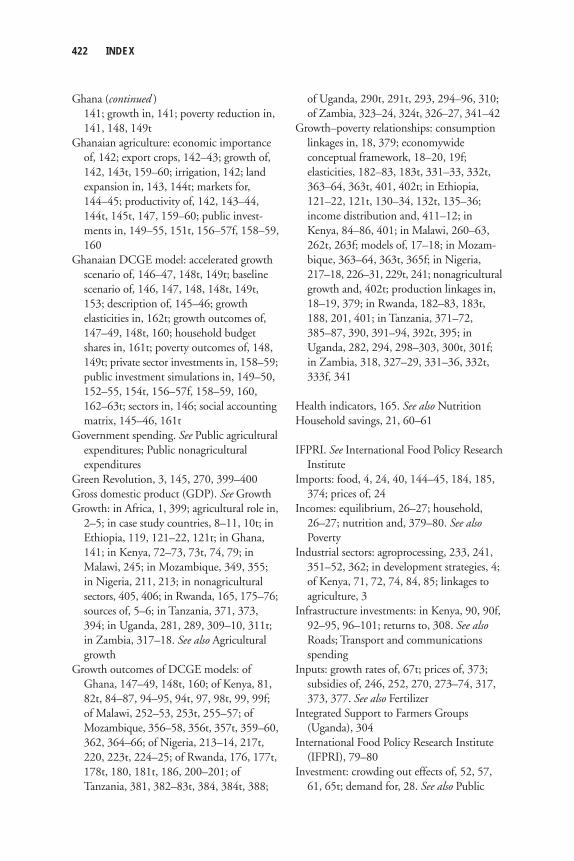
422 INDEX
Ghana (continued ) 141; growth in, 141; poverty reduction in,
141, 148, 149tGhanaian agriculture: economic importance
of, 142; export crops, 142–43; growth of, 142, 143t, 159–60; irrigation, 142; land expansion in, 143, 144t; markets for, 144–45; productivity of, 142, 143–44, 144t, 145t, 147, 159–60; public invest-ments in, 149–55, 151t, 156–57f, 158–59, 160
Ghanaian DCGE model: accelerated growth scenario of, 146–47, 148t, 149t; baseline scenario of, 146, 147, 148, 148t, 149t, 153; description of, 145–46; growth elasticities in, 162t; growth outcomes of, 147–49, 148t, 160; household budget shares in, 161t; poverty outcomes of, 148, 149t; private sector investments in, 158–59; public investment simulations in, 149–50, 152–55, 154t, 156–57f, 158–59, 160, 162–63t; sectors in, 146; social accounting matrix, 145–46, 161t
Government spending. See Public agricultural expenditures; Public nonagricultural expenditures
Green Revolution, 3, 145, 270, 399–400Gross domestic product (GDP). See GrowthGrowth: in Africa, 1, 399; agricultural role in,
2–5; in case study countries, 8–11, 10t; in Ethiopia, 119, 121–22, 121t; in Ghana, 141; in Kenya, 72–73, 73t, 74, 79; in Malawi, 245; in Mozambique, 349, 355; in Nigeria, 211, 213; in nonagricultural sectors, 405, 406; in Rwanda, 165, 175–76; sources of, 5–6; in Tanzania, 371, 373, 394; in Uganda, 281, 289, 309–10, 311t; in Zambia, 317–18. See also Agricultural growth
Growth outcomes of DCGE models: of Ghana, 147–49, 148t, 160; of Kenya, 81, 82t, 84–87, 94–95, 94t, 97, 98t, 99, 99f; of Malawi, 252–53, 253t, 255–57; of Mozambique, 356–58, 356t, 357t, 359–60, 362, 364–66; of Nigeria, 213–14, 217t, 220, 223t, 224–25; of Rwanda, 176, 177t, 178t, 180, 181t, 186, 200–201; of Tanzania, 381, 382–83t, 384, 384t, 388;
of Uganda, 290t, 291t, 293, 294–96, 310; of Zambia, 323–24, 324t, 326–27, 341–42
Growth–poverty relationships: consumption linkages in, 18, 379; economywide conceptual framework, 18–20, 19f; elasticities, 182–83, 183t, 331–33, 332t, 363–64, 363t, 401, 402t; in Ethiopia, 121–22, 121t, 130–34, 132t, 135–36; income distribution and, 411–12; in Kenya, 84–86, 401; in Malawi, 260–63, 262t, 263f; models of, 17–18; in Mozam-bique, 363–64, 363t, 365f; in Nigeria, 217–18, 226–31, 229t, 241; nonagricultural growth and, 402t; production linkages in, 18–19, 379; in Rwanda, 182–83, 183t, 188, 201, 401; in Tanzania, 371–72, 385–87, 390, 391–94, 392t, 395; in Uganda, 282, 294, 298–303, 300t, 301f; in Zambia, 318, 327–29, 331–36, 332t, 333f, 341
Health indicators, 165. See also NutritionHousehold savings, 21, 60–61
IFPRI. See International Food Policy Research Institute
Imports: food, 4, 24, 40, 144–45, 184, 185, 374; prices of, 24
Incomes: equilibrium, 26–27; household, 26–27; nutrition and, 379–80. See also Poverty
Industrial sectors: agroprocessing, 233, 241, 351–52, 362; in development strategies, 4; of Kenya, 71, 72, 74, 84, 85; linkages to agriculture, 3
Infrastructure investments: in Kenya, 90, 90f, 92–95, 96–101; returns to, 308. See also Roads; Transport and communications spending
Inputs: growth rates of, 67t; prices of, 373; subsidies of, 246, 252, 270, 273–74, 317, 373, 377. See also Fertilizer
Integrated Support to Farmers Groups (Uganda), 304
International Food Policy Research Institute (IFPRI), 79–80
Investment: crowding out effects of, 52, 57, 61, 65t; demand for, 28. See also Public
INDEX 423
agricultural expenditures; Public nonagricultural expenditures
Investment analysis: approaches to, 12–13; integration of, 410–11. See also individual countries
Irrigation: in Ghana, 142; in Kenya, 76, 92–94, 95, 97, 100; in Malawi, 270–71; in Rwanda, 192; in Tanzania, 374; in Zambia, 339–40
Iyaniwura, J., 213
Kakwani, N., 52Kelly, V., 174, 191Kenya: agroecological zones of, 76–79, 77f,
78t; development strategy of, 71–72, 73–75, 79, 86–87, 100; economic structure of, 77, 102t; growth in, 72–73, 73t, 74, 79; growth–poverty relationships in, 401; income inequality in, 86, 87; industrial sectors of, 71, 72, 74, 84, 85; infrastructure investments in, 90, 90f, 92–95, 96–101; metropolitan centers of, 77, 77f; poverty in, 73, 74, 74t, 78, 79, 97–98; roads in, 91–92, 96–97; rural economy of, 71, 75; rural population of, 75
Kenya Institute for Public Policy Research and Analysis (KIPPRA), 79–80
Kenyan agriculture: development role of, 72, 75–76, 79, 100; economic linkages of, 85; export crops, 75, 79, 87–89, 94–95, 96; fertilizer use in, 76; foodcrops, 75, 76, 78, 87, 88, 94; growth of, 72, 75–76; growth rate targets for, 71, 72, 75, 101; irrigation, 76, 92–94, 95, 97, 100; livestock and dairy sector, 79, 87, 88, 94; market access of, 76, 90, 96; productivity of, 75, 76, 89–90; public investments in, 75, 89–91, 90f, 100–101; regional differences in, 76–79, 78t; research and extension in, 75, 76, 90, 92–93, 94–95, 98, 100, 101
Kenyan DCGE model: accelerated growth scenarios of, 80, 81, 82t, 83t, 84–87; baseline scenario of, 80–81, 82t, 83t, 92, 103t; data sources for, 80, 92; development of, 79–80; growth incidence curves in, 86, 86f; growth outcomes of, 81, 82t, 84–87,
94–95, 94t, 97, 98t, 99, 99f; investment scenarios in, 72, 91–101, 93f, 94t, 95t, 98t, 99f; poverty outcomes of, 81, 83t, 84–87, 88, 89f, 95, 95t, 97, 97f, 98t, 99–100; sectoral growth multipliers in, 85, 85t; social accounting matrix, 79–80, 103t; subsectors in, 87–89, 89f
KIPPRA. See Kenya Institute for Public Policy Research and Analysis
Labor, in Ethiopian agriculture, 119–20, 123, 125
Labor markets, 43, 80Lin, L., 270Livestock and dairy sectors: calorie contents
of foods, 379–80; in Ethiopia, 116, 117, 122; in Kenya, 79, 87, 88, 94; in Mozam-bique, 352; in Nigeria, 224–25, 233–34; prices in, 184–85, 185f, 201, 379–80; in Rwanda, 169, 184–85, 185f; in Tanzania, 376–77, 393; in Uganda, 283, 286, 287t, 293
Malawi: development strategy of, 266, 269, 274; food security in, 246, 273–74; growth in, 245; growth–poverty relationships in, 260–63, 262t, 263f; land and population distribution in, 247–50, 249t, 274t; population growth in, 245; poverty in, 245, 246, 248–50, 273; roads in, 271–72; structural reforms in, 245–46; transport and communications spending in, 271–72, 272f
Malawian agriculture: constraints on growth of, 246, 263–64; districts, 247, 248f, 251; economic importance of, 247, 257; eco-nomic linkages of, 262–63, 264t; export crops, 247–48, 249t, 251, 259–60, 273, 403; farm sizes in, 247–50, 249t; farm typology in, 247–50; foodcrops, 246, 247, 249t, 251, 273, 403; growth of, 245–46,
272–74; input subsidies in, 246, 252, 270, 273–74, 377; irrigation, 270–71; prices in, 260, 263–64, 265f; productivity of, 246, 249t, 254t, 256–57, 256t, 265; public investments in, 266–72; research and extension in, 256, 270, 271f; in urban areas, 250
424 INDEX
Malawian DCGE model: accelerated growth scenarios of, 253t, 254t, 255–66; baseline scenario of, 252–55, 253t, 254t; data sources for, 251; description of, 250–52; farm typology in, 246–47, 251, 252; growth outcomes of, 252–53, 253t, 255–57; household income elasticities in, 252, 264, 275t; investment analysis of, 266–71, 268t, 273, 276t; poverty outcomes of, 253–55, 255f, 257–63, 258t, 262t, 263f, 265–66, 273; production linkages in, 251–52; social accounting matrix, 250–51, 275t; subsectors in, 259–63, 259f, 261f, 273
Malawi Growth and Development Strategy (MGDS), 269, 270–71, 272
Malley, Z. J. U., 377Malnutrition, in Tanzania, 372. See also Food
security; NutritionMaputo Declaration, 72, 90–91, 100, 101,
188. See also Comprehensive Africa Agriculture Development Programme; Public agricultural expenditures
Market access, 76, 90, 96, 407–8. See also Roads
Matsumoto, T., 377McCool, C., 354MDGs. See Millennium Development GoalsMeertens, B., 377MGDS. See Malawi Growth and
Development StrategyMilk. See Livestock and dairy sectorsMillennium Development Goals (MDGs),
51, 52, 81, 141, 309, 405. See also Poverty reduction
Mozambican agriculture: biofuel crops, 350, 352–54, 359–60, 364, 367; commercial plantations, 351, 352; constraints on growth of, 349–50, 352; economic importance of, 351; economic linkages of, 360, 362, 364–66, 365t; export crops, 350, 351, 359–61, 362, 364, 368t; fi sheries, 352; foodcrops, 351, 364, 367, 368t; foreign interest in, 350, 352; growth of, 349, 355–56, 366; investment priorities in, 350, 366–67; livestock and dairy sector, 352; productivity of, 350, 356–58, 357t, 359, 361–62; by province, 353t, 354, 360–61, 368t; smallholders in, 351
Mozambican DCGE model: accelerated growth scenarios of, 356t, 359–60, 361t; baseline scenario of, 355–58, 356t, 361t; consumption expenditures in, 355; data sources for, 354; description of, 354–55; growth outcomes of, 356–58, 356t, 357t, 359–60, 362, 364–66; poverty outcomes of, 358, 358f, 360–62, 361t, 363–66; price effects in, 355, 361, 362, 362f; social accounting matrix, 354, 369t; subsectors in, 354, 363–66, 363t, 365f
Mozambique: agroprocessing industries in, 351–52, 362; civil war effects in, 349, 356; development strategy of, 349; food security in, 349; growth in, 349, 355; growth–poverty relationships in, 363–64, 363t, 365f; land and population distribution in, 351–52, 353t; poverty in, 349
National Agricultural Advisory Services (NAADS; Uganda), 304, 307–8
National Development Plan (NDP; Kenya), 73–75
National Economic Empowerment and Development Strategies (NEEDS; Nigeria), 212
National Food Security Program (NFSP; Nigeria), 212, 219–20, 224
Ndayizigiye, F., 174NDP. See National Development PlanNEEDS. See National Economic Empower-
ment and Development StrategiesNew Partnership for Africa’s Development
(NEPAD), 2. See also Comprehensive Africa Agriculture Development Programme
NFSP. See National Food Security ProgramNigeria: agroprocessing industries in, 233,
241; development strategy of, 211, 212, 241, 242; food security in, 212; growth in, 211, 213; growth–poverty relationships in, 217–18, 226–31, 229t, 241; incomes in, 232; investment in, 214; oil exports of, 211, 213, 214; poverty in, 211, 216–19, 218f, 219f, 226; poverty reduction in, 212; public nonagricultural expenditure in, 234–36, 237–38, 240; rural population of, 212; state governments of, 241
Nigerian agriculture: economic importance of, 211, 212; export crops, 224, 231; food-
INDEX 425
crops, 220, 224, 230–31, 233; growth in, 211, 213–14; growth targets of, 212, 219; livestock and dairy sector, 224–25, 233–34; markets for, 240–41; productivity of, 215, 220, 221–22t; public investments in, 234, 236–40, 239f, 241–42
Nigerian DCGE model: accelerated growth scenarios of, 215t, 217t, 219–20, 221–22t, 223t, 224–34; baseline scenario of, 213–19, 215t, 217t, 221–22t, 223t; capital accumulation in, 214; data sources for, 213; description of, 212–13; growth decomposition in, 214–16, 215t; growth multipliers in, 230–31; growth outcomes of, 213–14, 217t, 220, 223t, 224–25; investment analysis of, 234–40, 237t; poverty outcomes of, 216–19, 218f, 219f, 225–31, 225f, 227t; price effects in, 231–34, 232f; social accounting matrix, 213, 242t; subsectors in, 212–13, 220, 223t, 224–25, 228–31, 240–41
Nin Pratt, A., 338Nutrition: caloric availability, 39, 379–80,
380t; growth relationship, 379, 390–91, 392t; incomes and, 379–80; in Tanzanian DCGE model, 379–81, 384–85, 386t, 390–91, 412. See also Food
Nyanga, D., 377–78
PAE. See Public agricultural expendituresPASDEP. See Plan for Accelerated and
Sustained Development to End PovertyPiesse, J., 270Plan for Accelerated and Sustained Develop-
ment to End Poverty (PASDEP; Ethiopia), 110, 115–16, 137
Plan for the Modernisation of Agriculture (PMA; Uganda), 282, 304
PNE. See Public nonagricultural expendituresPopulation growth: in Africa, 204; in Malawi,
245; in Uganda, 282; in Zambia, 317Poultry. See Livestock and dairy sectorsPoverty: in Africa, 1–2, 399; consumption
function and, 38–39; defi nition of, 412; in Ethiopia, 121–22, 121t, 130–31, 132t, 133t; increases in, 1; in Kenya, 73, 74, 74t, 78, 79, 97–98; in Malawi, 245, 246, 248–50, 273; measures of, 48n, 411, 412; in Mozambique, 349; in Nigeria,
211, 216–19, 218f, 219f, 226; in rural areas, 2, 3, 4, 6–8; in Rwanda, 166; social protection policies and, 413; in Tanzania, 371–72, 385, 395, 409; in Uganda, 281–82, 311t. See also Growth–poverty relationships
Poverty outcomes of DCGE models: of Ethiopia, 121, 122, 130–34, 132t, 133t, 135–36; of Ghana, 148, 149t; of Kenya, 81, 83t, 84–87, 88, 89f, 95, 95t, 97, 97f, 98t, 99–100; of Malawi, 253–55, 255f, 257–63, 258t, 262t, 263f, 265–66, 273; of Mozambique, 358, 358f, 360–62, 361t, 363–66; of Nigeria, 216–19, 218f, 219f, 225–31, 225f, 227t; of Rwanda, 176, 179, 180–83, 181t, 186, 201; of Tanzania, 385–87, 386t, 389–90; of Uganda, 293–94, 294f, 296–98, 297t, 310; of Zambia, 324–26, 326f, 327–36, 330t, 341
Poverty reduction: agricultural growth’s role in, 2, 4, 87, 167, 401–2, 402t, 405–6; in case study countries, 10–11, 11t; in Ethiopia, 110, 131–34, 132t; export crops and, 4, 402–5, 404t; foodcrops and, 402–5, 404t; in Ghana, 141, 148, 149t; in Nigeria, 212; obstacles to, 1–2; in Rwanda, 176, 179, 186, 200; in Uganda, 281–82, 304, 309–10. See also Millennium Development Goals
Price effects in DCGE models: of Mozam-bique, 355, 361, 362, 362f; of Nigeria, 231–34, 232f; of Rwanda, 183–85, 201–2; of Tanzania, 388–89, 389f; of Uganda, 298, 299f
Prices: equilibrium, 26, 27; in Ethiopian agriculture, 129–30, 129t, 133–34, 135; of exports, 25; of food, 133–34, 135, 184, 184f, 231–34, 298, 379–80; growth links of, 183–85, 201–2, 231–34; of imports, 24; of inputs, 373; of livestock products, 184–85, 185f, 201; in Malawi, 260, 263–64, 265f; marketing costs and, 33; producer, 23; in Rwanda, 183–85, 201–2; in Tanzania, 373
Productivity, agricultural: in Ethiopia, 115, 136; in Ghana, 142, 143–44, 144t, 145t, 147, 159–60; in Kenya, 75, 76, 89–90; in Malawi, 246, 249t, 254t, 256–57, 256t,
426 INDEX
Productivity, agricultural (continued ) 265; in Mozambique, 350, 356–58, 357t, 359, 361–62; in Nigeria, 215, 220, 221–22t;
in Rwanda, 166, 167, 168, 176, 177t, 192, 195t, 196, 197, 200; in Tanzania, 373, 381, 382–83t, 395; in Uganda, 282, 290, 292, 295–96, 295t; in Zambia, 324, 325t, 326–27, 327t, 328. See also Total factor productivity
PSTA. See Strategic Plan for Agricultural Transformation in Rwanda
Public agricultural expenditures (PAE): agricultural growth sources and, 55–56; application of estimation formula, 60; constraints on, 205, 408; crowding out effects of, 52, 57, 61, 65t; data sources for estimation of, 57–60; effi ciency of, 408–9; elasticity of output and, 59, 63t, 64t, 266–67; estimation approaches, 51–52; estimation parameters, 58t; in Ethiopia, 109–10, 113, 136; in export crop sectors, 203–4; externalities of, 189; fi nancing of, 60–62; in Ghana, 149–55, 151t, 156–57f, 158–59, 160; growth of, 56, 66t; increasing, 408–9; interaction effects of, 65t; interaction with nonagricultural spending, 52, 54, 56, 57, 59; in Kenya, 75, 89–91, 90f, 100–101; in Malawi, 266–72; Maputo Declaration targets, 72, 90–91, 101, 188; in Nigeria, 234, 236–40, 239f, 241–42; potential returns to, 189–92, 196–99, 198t, 202–4; prioritizing, 189, 269–72, 298–304, 303f, 306–7; private sector investments and, 158–59; pro-ductivity impact of, 89–92, 92t; required to achieve agricultural growth rates, 57; returns to, 91, 92t, 270, 272, 304, 307, 308, 402; rural infrastructure investments, 90, 308; in Rwanda, 185–92, 187t, 190t, 193–94t, 196–99, 202–4; in Tanzania, 377–78, 395; in Uganda, 282, 304–8, 307f, 310–11, 409; in Zambia, 336–38, 339–41, 342
Public nonagricultural expenditures (PNE): effects of, 52, 64t; effi ciency of, 408–9; elasticities of, 64t; growth of, 56; inter-action with agricultural spending, 52, 54, 56, 57, 59; in Malawi, 271–72; in Nigeria,
234–36, 237–38, 240; returns to, 272; in Uganda, 304–6
Public spending, 54–55, 56, 66t
Rao, N., 377–78REMA. See Rwandan Environment
Management AuthorityResearch and extension services: in Ethiopia,
109–10, 113; in Kenya, 75, 76, 90, 92–93, 94–95, 98, 100, 101; in Malawi, 256, 270, 271f; returns to investment in, 270, 308, 377–78, 411; in Tanzania, 377–78, 395; in Uganda, 270, 304, 307–8, 307f, 411; in Zambia, 318, 338–39, 339f
Risk, 413Roads: in Ethiopia, 136; in Kenya, 91–92,
96–97; in Malawi, 271–72; in Tanzania, 395; in Uganda, 272, 306, 308, 340; in Zambia, 340–41. See also Transport and communications spending
Roose, E., 174Rosegrant, M. W., 339Rural poverty, 2, 3, 4, 6–8. See also PovertyRwanda: budget allocations in, 188–89, 191;
development challenges of, 166; develop-ment strategies of, 166, 171–73, 189–91, 200; education in, 165; food consumption spending in, 169–70, 175, 184; food imports of, 184, 185; food security in, 170, 173, 179, 201; genocide effects in, 165, 166, 168, 175; growth in, 165, 175–76; growth–poverty relationships in, 182–83, 183t, 188, 201, 401; health indicators in, 165; nonagricultural trade of, 185; popu-lation density of, 167–68; population distribution of, 169, 170t; poverty in, 166; poverty reduction in, 176, 179, 186, 200; private investment in, 186; public and private investment in, 165
Rwandan agriculture: comparisons to other countries, 204–5; by district, 171; economic importance of, 167; economic linkages of, 203; environmental sustainability of, 168, 172; export crops, 167, 168–69, 170–71, 172, 175, 182, 185, 199, 203–4; fertilizer use in, 172, 191, 192; foodcrops, 169, 170, 182–83, 184, 201, 203; growth of, 167–68, 175–76, 177t, 178t, 192, 199,
INDEX 427
200; incomes in, 167, 168, 169; irrigation, 192; landholding sizes in, 169, 170t; land scarcity in, 168, 169, 204; livestock and dairy sector, 169, 184–85, 185f; previous research on, 173–74; prices in, 183–85, 184f, 185f, 201–2; productivity of, 166, 167, 168, 176, 177t, 192, 195t, 196, 197, 200; public investments in, 185–92, 187t, 190t, 193–94t, 196–99, 202–4; soil erosion and, 168, 172, 173–74; subsistence, 168
Rwandan DCGE model: accelerated growth scenarios of, 179–85, 181t; baseline scenario of, 175–76, 177t, 178t, 179; description of, 174–75; growth outcomes of, 176, 177t, 178t, 180, 181t, 186, 200–201; investment analysis of, 185–92, 196–99; poverty outcomes of, 176, 179, 180–83, 181t, 186, 201; price effects in, 183–85, 201–2; social accounting matrix, 174–75, 206t
Rwandan Environment Management Authority (REMA), 168
SAMs. See Social accounting matrixesSaurkar, A., 236SDPRP. See Sustainable Development and
Poverty Reduction ProgramSocial accounting matrixes (SAMs), 34–37,
35t, 42Social protection policies, 413Son, H. H., 52South Africa, 8Staple crops. See FoodcropsStrategic Plan for Agricultural Transformation
in Rwanda (PSTA), 172–73Sub-Saharan Africa. See AfricaSubsidies: fertilizer, 110, 270, 338; input,
246, 252, 270, 273–74, 317, 373, 377Sustainable Development and Poverty
Reduction Program (SDPRP; Ethiopia), 110
Taeb, M., 377Tanzania: development strategy of, 376–77,
378; food imports of, 374; growth in, 371, 373, 394; growth–poverty relationships in, 371–72, 385–87, 390, 391–94, 392t,
395; income inequality in, 371, 395; malnutrition in, 372; poverty in, 371–72, 385, 395, 409; roads in, 395; structural adjustment policies of, 373–74, 377
Tanzanian agriculture: constraints on growth of, 377; economic linkages of, 392–94, 393t; export crops, 375t, 376, 387, 393; fertilizer use in, 373, 377; fi sheries, 376; foodcrops, 374–76, 375t; growth of, 372, 373, 374–76, 387; growth potential of, 376–78; input prices in, 373; input subsidies in, 373, 377; investment priorities in, 393–94, 394f, 395; irrigation, 374; livestock and dairy sector, 376–77, 393; prices in, 373; productivity of, 373, 381, 382–83t, 395; public investments in, 377–78, 395; regions of, 378, 387; research and extension in, 377–78, 395; technology in, 373, 374, 377
Tanzanian DCGE model: accelerated growth scenarios of, 382–83t, 384t, 387–94; base-line scenario of, 381, 382–83t, 384–87, 384t; data sources for, 378, 381; description of, 378–81; growth outcomes of, 381, 382–83t, 384, 384t, 388; growth source comparison in, 391–94, 393t; nutrition module of, 379–81, 384–85; nutrition outcomes of, 385, 386t, 390–91, 412;
poverty module of, 378–79, 384–85; poverty outcomes of, 385–87, 386t, 389–90; price effects in, 388–89, 389f; social accounting matrix, 378, 396t
Taxes, 19, 27–28, 52, 60–61TFP. See Total factor productivityThailand, exports of, 233–34Thirtle, C., 270Thurlow, J., 116, 354Total factor productivity (TFP): changes in,
53; determinants of growth of, 54, 56; growth in, 67t, 215, 216, 220; investment impacts on, 91, 92t; shocks to, 196. See also Productivity
Trade. See Export crops; ImportsTransaction costs, 33Transport and communications spending: in
Malawi, 271–72, 272f; in Uganda, 308, 309f; in Zambia, 340–41, 340f. See also Roads
428 INDEX
Uganda: development strategy of, 282, 304; education in, 411; food prices in, 298,
299f; growth in, 281, 289, 309–10, 311t; growth–poverty relationships in, 282, 294, 298–303, 300t, 301f; population growth in, 282; poverty in, 311t; poverty reduction in, 281–82, 304, 309–10; returns to public investment in agriculture in, 91, 92t, 270, 272, 304, 307, 308; roads in, 272, 306, 308, 340; transport and communications spending in, 308, 309f
Ugandan agriculture: economic linkages of, 301–2, 302t; export crops, 281, 283–86, 288, 292–93, 299, 310; farm typology in, 283–87, 284f, 285t, 288; fertilizer use in, 307; fi sheries and forestry, 293; foodcrops, 281, 283–84, 286, 288, 292; growth of, 281, 289, 309–10; livestock and dairy sector, 283, 286, 287t, 293; productivity of, 282, 290, 292, 295–96, 295t; public invest-ments in, 282, 304–8, 307f, 310–11, 409; research and extension in, 270, 304, 307–8, 307f, 411; in urban areas, 286–87, 298
Ugandan DCGE model: accelerated growth scenarios of, 290t, 291t, 294–98; baseline scenario of, 289–94, 290t, 291t; data sources for, 289; description of, 287–89; farm typology in, 288; growth outcomes of, 290t, 291t, 293, 294–96, 310; investment analysis of, 304–8, 305t, 313t; poverty outcomes of, 293–94, 294f, 296–98, 297t, 310; price effects in, 298, 299f; social accounting matrix, 312t; subsectors in, 287–88, 310, 312t
Verpoorten, M., 174Vision 2020 (Rwanda), 166, 171–72Vision 2030 (Kenya), 74Von Braun, J., 174
Wobst, P., 251Wolter, D., 377World Bank, 175, 270
Yields. See ProductivityYu, B., 236, 338
Zambia: agroecological zones of, 319, 322, 323; development strategy of, 336, 339–41; economic reforms in, 317; growth in, 317–18; growth–poverty relationships in, 318, 327–29, 331–36, 332t, 333f, 341; population growth in, 317; poverty reduction in, 317–18; roads in, 340–41; transport and communications spending in, 340–41, 340f
Zambian agriculture: constraints on growth of, 318; economic importance of, 319; eco-nomic linkages of, 331, 333–34, 335t, 341; export crops, 317, 319, 322, 328, 331, 334, 341; farm typology in, 319–22, 320f, 321t, 343t; fertilizer subsidies in, 338; fertilizer use in, 318; foodcrops, 317, 319–22, 332, 341–42; growth of, 317–18; investment priorities in, 334–36, 335f, 338–41; irrigation, 339–40; productivity of, 324, 325t, 326–27, 327t, 328; public investments in, 336–38, 339–41, 342; research and extension in, 318, 338–39, 339f; structural reforms in, 317; in urban areas, 322
Zambian DCGE model: accelerated growth scenarios of, 324t, 326–36; baseline scenario of, 323–24, 324t; data sources for, 323; description of, 323; growth outcomes of, 323–24, 324t, 326–27, 341–42; growth sources in, 328–31, 329f, 330f; investment analysis of, 336–41, 337t, 344t; poverty outcomes of, 324–26, 326f, 327–36, 330t, 341; social accounting matrix, 323, 344t; subsectors in, 323, 331–36, 341
Zhang, X., 91, 272, 304, 306, 307, 308, 340, 411
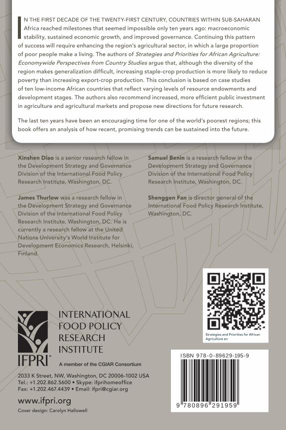
Working Multisectorally in Nutrition en
2033 K Street, NW, Washington, DC 20006-1002 USA
Fax: +1.202.467.4439 • Email: [email protected]
www.ifpri.orgCover design: Carolyn Hallowell
IN THE FIRST DECADE OF THE TWENTY-FIRST CENTURY, COUNTRIES WITHIN SUB-SAHARAN
Africa reached milestones that seemed impossible only ten years ago: macroeconomic
stability, sustained economic growth, and improved governance. Continuing this pattern
of success will require enhancing the region’s agricultural sector, in which a large proportion
of poor people make a living. The authors of Strategies and Priorities for African Agriculture: Economywide Perspectives from Country Studies argue that, although the diversity of the
poverty than increasing export-crop production. This conclusion is based on case studies
in agriculture and agricultural markets and propose new directions for future research.
The last ten years have been an encouraging time for one of the world’s poorest regions; this
book offers an analysis of how recent, promising trends can be sustained into the future.
Xinshen Diao is a senior research fellow in the Development Strategy and Governance Division of the International Food Policy Research Institute, Washington, DC.
James Thurlow was a research fellow in the Development Strategy and Governance Division of the International Food Policy Research Institute, Washington, DC. He is currently a research fellow at the United Nations University’s World Institute for Development Economics Research, Helsinki, Finland.
Samuel Benin is a research fellow in the Development Strategy and Governance Division of the International Food Policy Research Institute, Washington, DC.
Shenggen Fan is director general of the International Food Policy Research Institute, Washington, DC.
ISBN 978-0 -89629-195-9
9 7 8 0 8 9 6 2 9 1 9 5 9
Strategies and Priorities for African Agriculture en