Strategic Interactions in a Supply Chain Game

Michael P. Wellman Joshua Estelle Satinder SinghYevgeniy Vorobeychik Christopher Kiekintveld

Vishal SoniUniversity of Michigan

Artificial Intelligence LaboratoryAnn Arbor, MI 48109-2110 USA

� wellman, jestelle, baveja, yvorobey, ckiekint, soniv �@umich.edu

November 10, 2004

To appear in Computational Intelligence

Abstract

The TAC 2003 supply-chain game presented automated trading agents witha challenging strategic problem. Embedded within a high-dimensional stochasticenvironment was a pivotal strategic decision about initial procurement of compo-nents. Early evidence suggested that the entrant field was headed toward a self-destructive, mutually unprofitable equilibrium. Our agent, Deep Maize, intro-duced a preemptive strategy designed to neutralize aggressive procurement, per-turbing the field to a more profitable equilibrium. It worked. Not only did preemp-tion improve Deep Maize’s profitability, it improved profitability for the wholefield. Whereas it is perhaps counterintuitive that action designed to prevent oth-ers from achieving their goals actually helps them, strategic analysis employingan empirical game-theoretic methodology verifies and provides insight about thisoutcome.

1 Introduction

Like classic computer games, multiagent research competitions [Stone, 2002] presentwell-defined problems for testing and comparing AI techniques and systems. The an-nual Trading Agent Competition (TAC) series provides a forum for research on strate-gic market behavior, and has led to several promising concepts and methods for imple-menting strategies in such domains [Wellman et al., 2003].

The TAC Supply Chain Management (TAC/SCM) scenario [Arunachalam and Sadeh,to appear, Sadeh et al., 2003] defines a complex six-player game with severely incom-plete and imperfect information, and high-dimensional strategy spaces. Like the realsupply-chain environments it is intended to model, the TAC/SCM game presents par-ticipants with challenging decision problems in a context of great strategic uncertainty.

1

This paper is a case study of a strategic issue that arose in the first TAC/SCM tour-nament. We present our reasoning about the issue, and our effort to perturb the envi-ronment from an “equilibrium” we considered undesirable, to another more profitabledomain of operation. We recount the experience as it played out in the competition,and analyze the outcome of this naturalistic experiment. We then perform a more con-trolled experimental analysis of the issue, applying empirical game-theoretic methodsto produce compelling results, narrow in scope but arguably accounting well for strate-gic interactions.

The direct result of this study is validation of the insight behind our particularpolicy for strategic procurement in the TAC/SCM game. Our experimental analysisverifies that the predominant patterns we observed among agents in the tournamentreflect strategically rational behavior for this issue. It also confirms the surprising phe-nomenon in which a tactic designed to preempt the actions of others actually leadsto global welfare improvements. More broadly, we view this exercise as illustratinga general approach by which agent designers can reason through pivotal strategic is-sues in a principled way, despite computational and analytical intractability of theirenvironments.

2 Strategic Analysis for Complex Domains

Given the significant strategic interactions in the supply-chain game, we as agent de-signers would naturally like to apply game-theoretic tools to predict the behavior ofother agents, individually and in aggregate. Unfortunately, direct solution of the fullgame in the sense of finding equilibria (of any variety) seems out of the question ontractability grounds. Therefore, we seek other ways to exploit the concepts and meth-ods of game theory, short of comprehensive solutions.

The economic literature on game-theoretic applications is full of highly abstracted,or stylized models,1 designed to highlight some particular strategic issue of interest,suppressing or holding constant—in extremely summarized form—the many other fac-tors that would actually be present in any real instance of the modeled scenario. In gen-eral, these unmodeled factors may well be relevant to strategic decisions of the players.In suppressing them, the modeler is judging that the effect of these factors would notinteract so much as to invalidate the key strategic implications of the modeled factors.

We aim to employ a similarly reasoned use of abstraction, but in a situation wherea completely detailed description of the game is actually available. Whereas this avail-ability does not obviate the need for abstraction or other simplifying approximations,it does present opportunities for calibration and validation that may not exist when themodeler is abstracting the real world directly. For instance, we can often summarizethe unmodeled features analytically or through statistical simulation, and can achievesome validation through sensitivity analysis or comparison of alternative models basedon different simplifying assumptions.

TAC/SCM is an example of a very detailed model intended to capture aspects ofa real situation, offering the prospect that interesting phenomena may emerge from

1For example, peruse any text on game theory [Fudenberg and Tirole, 1991, Gintis, 2000] for a wealth ofsuch enlightening examples.

2

interactions of the details, even if unanticipated by designers. Given a game in thisform, analysts may form hypotheses about identified features of interest based on rea-soning (about the game specification) and observation (of actual game instances), andthen construct a more abstracted model focusing on these features. After using thedetailed model to quantify the abstracted model, one can solve the abstracted modelusing standard techniques.

In this study, we construct such a model by estimation applied to data from simu-lations. Its basis in a sampled experience renders this model an empirical game. Sincethe empirical game considers only a limited repertoire of strategies, it also constituteswhat Walsh et al. [2003] term a heuristic strategy payoff matrix. The approach we taketo construction and analysis of this model builds on our previous application of empiri-cal game-solving methodology [Reeves et al., to appear]. It shares much in motivationand operation with the constrained-equilibrium approach advocated by Armantier et al.[2000], as well as the approach to various strategic environments explored by Kephartand colleagues [Kephart and Greenwald, 2002, Kephart et al., 1998, Walsh et al., 2002].

The present study contributes several elements to this emerging empirical game-theoretic approach. First, we employ standard variance-reduction techniques, in par-ticular the method of control variates, to reduce the amount of simulation required toobtain statistically meaningful results. Second, from the empirical game we deriveboth symmetric (mixed strategy) and non-symmetric (pure strategy) Nash equilibria.We employ statistical hypothesis testing as well as analysis of the benefits from devia-tion as means to assess the stability of candidate strategy profiles.

Our investigation of strategic procurement in TAC/SCM illustrates more generallyhow the combination of gaming, simulation, experimental manipulation, and game-theoretic analysis can provide insight into a complex strategic environment. We be-lieve that these methods comprise a promising methodology for problems charac-terized by significant dynamics and uncertainty, with fine-grained interaction amongagents. Real-world commerce environments (e.g., supply chains) very often exhibitthese features. For such problems, comprehensive direct analysis of detailed mod-els is intractable, but ex ante stylization risks abstracting away pivotal features. Ourmethodology does not completely avoid these risks, but increases confidence throughvalidation based on maintaining an explicit bridge between the detailed and stylizedmodels.

3 TAC/SCM Game

In the TAC/SCM scenario,2 six agents representing PC (personal computer) assemblersoperate in a common market environment, over a simulated production horizon. Theenvironment constitutes a supply chain, in that agents trade simultaneously in marketsfor supplies (PC components) and the market for finished PCs. Agents may assemblefor sale 16 different models of PCs, defined by the compatible combinations of the four

2For complete details of the game rules, see the specification document [Arunachalam et al., 2003]. Thisis available athttp://www.sics.se/tac, as is much additional information about TAC/SCM and TACin general. Arunachalam and Sadeh [to appear] discuss the challenges posed by the game, and present anaccount of the 2003 tournament.

3

component types: CPU, motherboard, memory, and hard disk.Figure 1 diagrams the basic configuration of the supply chain. The six agents (ar-

rayed vertically in the middle of the figure) procure components from the eight suppli-ers on the left, and sell PCs to the entity representing customers, on the right. Trades atboth levels are negotiated through a request-for-quote (RFQ) mechanism, which pro-ceeds in three steps:

1. Buyer issues RFQs to one or more sellers.

2. Sellers respond to RFQs with offers.

3. Buyers accept or reject offers. An accepted offer becomes an order.

The suppliers and customer implement fixed negotiation policies, defined in the gamespecification, and discussed in detail below where applicable.

Agent 1

Agent 2

Agent 4

Agent 3

Agent 5

Agent 6

Pintel

IMD

Basus

Macrostar

Mec

Queenmax

Watergate

Mintor

supplieroffer

componentRFQ

offeracceptance

Customerbid

PC RFQ

CPU

Mot

herb

oard

Mem

ory

Har

d D

isk

Figure 1: TAC/SCM supply chain.

The game runs for 220 simulated days. On each day, the agent may receive of-fers and component delivery notices from suppliers, and RFQs and offer acceptancenotifications from customers. It then must make several decisions:

1. What RFQs to issue to component suppliers.

2. Given offers from suppliers (based on the previous day’s RFQs), which to accept.

3. Given component inventory and factory capacity, what PCs to manufacture.

4. Given inventory of finished PCs, which customer orders to ship.

5. Given RFQs from customers, to which to respond and with what offers.

In the simulation, the agent has 15 seconds to compute and communicate its dailydecisions to the game server. At the end of the game, agents are evaluated by totalprofit, with any outstanding component or PC inventory valued at zero.

As we describe below, a key stochastic feature of the game environment is level ofdemand for PCs. The underlying demand level is defined by an integer parameter �

4

(called ������ in the specification document [Arunachalam et al., 2003, Section 6]).

Each day, the customer issues a set of �� RFQs, where �� is drawn from a Poissondistribution with mean value defined by the parameter � for that day. Since the orderquantity, PC model, and reserve price are set independently for each customer RFQ,the number of RFQs serves as a sufficient statistic for the overall demand, which inturn is a major determinant of the potential profits available to the agents.

The demand parameter � evolves according to a given stochastic process. In eachgame instance, an initial value, ��, is drawn uniformly from [80,320]. If �� is thevalue of � on day �, then its value on the next day is given by [Arunachalam et al.,2003, Section 6]:

���� � ������������� ������� (1)

where � is a trend parameter that also evolves stochastically. The initial trend is neutral,�� � , with subsequent trends updated by a perturbation � � � ����� � ��� �:

���� � ����������� ������ �� � ���� (2)

In a given game, the demand may stay at predominantly high or low levels, or oscillateback and forth. The probabilistic behavior of � figures importantly in our analysis, aspresented in Section 7 below.

Although it necessarily simplifies the PC market and manufacturing process to agreat extent, the TAC/SCM game does introduce several realistic elements not typicallyincorporated in trading games. Specifically, it embeds trading in a concrete productioncontext, and incorporates stochastic (and partially observable) exogenous effects. Likeactors on real supply chains, TAC/SCM agents make decisions under uncertainty overtime, dealing with both suppliers and customers, in a competitive market environment.Negotiation concerns several facets of a deal (price, quantity, delivery time, penalty),and takes place simultaneously at multiple tiers.

4 Deep Maize

The University of Michigan’s entry in TAC-03/SCM is an agent called Deep Maize[Kiekintveld et al., 2004a,b]. The agent is organized in modular functional units con-trolling procurement, manufacturing, and sales. Its behavior is based on distributedfeedback control, in that it acts to maintain a reference zone of profitable operation.To coordinate the distributed modules, Deep Maize employs aggregate price signals,derived from a market equilibrium analysis and continual Bayesian demand projection.The design of Deep Maize optimizes for performance in the steady state, with littleexplicit attention to transient or end-game behaviors.

In the present study we focus on one pivotal feature of Deep Maize’s strategy,described in full detail below. We thus defer specifics of the rest of our agent’s strategyto our other reports (which in turn do not address the strategic analysis presented here).

5

5 Day-0 Procurement Strategies

A close examination of the game rules suggests that procurement of components atthe very beginning of the game (day-0 procurement) may be a pivotal strategic is-sue. This was indeed borne out by the behavior observed in preliminary rounds of thetournament, as discussed below. In this section, we explain the reason for expectingday-0 procurement to be so significant, and its ramifications for Deep Maize and otheragents.

5.1 Supplier Pricing

In the TAC/SCM market, suppliers set prices for components based on an analysisof their available capacity. Conceptually, there exist separate prices for each type ofcomponent, from each supplier. Moreover, these prices vary over time: both the timethat the deal is struck, and time that the component is promised for delivery.

The TAC/SCM component catalog [Arunachalam et al., 2003, Figure 3] associatesevery component � with a base price, �. The correspondence between price and quan-tity for component supplies is defined by the suppliers’ pricing formula [Arunachalamet al., 2003, Section 5.5]. The price offered by a supplier at day � for an order to bedelivered on day �� is

����� � � � � ��������� �

���� (3)

where for any , ��� � denotes the cumulative capacity for � the supplier projects tohave available from the current day through day . The denominator, ���, representsthe nominal capacity controlled by the supplier over days, not accounting for anycapacity committed to existing orders.

Supplier prices according to Eq. (3) are date-specific, depending on the particularpattern of capacity commitments in place at the time the supplier evaluates the givenRFQ. A key observation is that component prices are never lower than at the start of thegame (� � �), when ���� � ��� and therefore ���� � ����, for all � and .3 As thesupplier approaches fully committed capacity (���� � � � �), ���� � � approaches�.

In general, one would expect that procuring components at half their base pricewould be profitable, up to the limits of production capacity. Customer reserve pricesrange between 0.75 and 1.25 the base price of PCs, defined as the sum of base prices ofcomponents. Therefore, unless there is a significant oversupply, prices for PCs shouldeasily exceed the component cost, based on day-0 prices.

An agent’s procurement strategy must also take into account the specific TAC/SCMRFQ process. Each day, agents may submit up to 10 RFQs, ordered by priority, toeach supplier. The suppliers then repeatedly execute the following, until all RFQs are

3As discussed below, this creates a powerful incentive for early procurement, with significant conse-quences for game balance. In retrospect, the supplier pricing rule was generally considered a design flaw inthe game, and has been substantially revised for the 2004 TAC/SCM tournament.

6

exhausted: (1) randomly choose an agent,4 (2) take the highest-priority RFQ remainingon its list, (3) generate a corresponding offer, if possible. In responding to an RFQ, ifthe supplier has sufficient available capacity to meet the requested quantity and duedate, it offers to do so according to its pricing function. If it does not, the supplierinstead offers a partial quantity at the requested date and/or the full quantity at a laterdate, to the best of its ability given its existing commitments. In all cases, the supplierquotes prices based on Eq. (3), and reserves sufficient capacity to meet the quantity anddate offered.

5.2 Implications of Aggressive Day-0 Procurement

From the discussion above, it would appear advantageous to any agent that it attempt toprocure a large number of components on day 0. We call this strategy aggressive day-0 procurement, or simply aggressive. From each agent’s perspective, the main effectof being aggressive is on its own component procurement profile. If every agent isaggressive, however, it can significantly change the character of the game environment.

An aggressive day-0 procurement commits to large component orders before over-all demand over the game horizon is known. This leaves agents with little flexibilityto respond to cases of low demand, except by lowering PC prices to customers. Sincecomponent costs are sunk at the beginning, there is little to keep prices from droppingbelow (ex ante) profitable levels. Ketter et al. [2004] confirm the importance of day-0procurement in determining overall performance, finding a strong positive correlationbetween components obtained on day 0 and profitability for high-demand games, anda negative correlation for games characterized by low demand.

As more agents procure aggressively, several factors make aggressiveness evenmore compelling. The aggressive agents reserve significant fractions of supplier capac-ity, thus reducing subsequent availability and raising prices, according to their pricingfunction (3). A natural response might induce a “race” dynamic, where agents issueday-0 RFQs in increasingly large chunks, ultimately requesting all components theyexpect to be able to use over the entire game horizon. Not only does this exacerbatethe risk of locking in aggregate oversupply, it also produces a less interleaved and moreunbalanced distribution of components, especially at the beginning of the game. Thisin turn can prevent many agents from being able to acquire key components needed forparticular PC models until relatively far into the production year.

For all these reasons, the aggressive strategy is appealing to individual agents, yetpotentially quite damaging for the agent pool overall. We considered this situationparticularly bad for our agent, given that it was designed for high performance in thesteady state [Kiekintveld et al., 2004a]. Deep Maize devotes a considerable efforttoward developing accurate demand projections, and thus is quite responsive to actualdemand conditions. If most of the game’s component procurement is up front, wenever reach a steady state, and the ability to respond to demand conditions is much lessrelevant.

4At the start of the game, suppliers select among agents with equal probability. Thereafter, suppliersemploy a reputation mechanism whereby the probability of agent choice depends on its record of acceptingprevious offers. We discuss the operation and effectiveness of this mechanism in Section 6.2.

7

Agent Affiliation Average Profit ($M)Qualifying Seeding 1 Seeding 2

TacTex U Texas 33.65 32.66 32.97RedAgent McGill U 15.09 24.57 29.52Botticelli Brown U 13.88 17.29 28.03Jackaroo U Western Sydney 14.89 35.55 19.23WhiteBear Cornell U –3.17 13.57 16.50PSUTAC Pennsylvania State U –120.0 15.52 15.25HarTAC Harvard U 12.41 4.19 10.72UMBCTAC U Maryland Baltimore Cty –13.94 30.16 10.23Sirish –109.4 –0.17 8.27Deep Maize U Michigan 1.85 0.45 7.49TAC-o-matic Uppsala U 0.22 1.79 7.07RonaX Xonar GmbH –0.92 9.24 4.29MinneTAC U Minnesota 10.88 6.56 –0.32Mertacor Aristotle U Thessaloniki 9.29 –0.38 –3.53zepp Poli Bucharest –24.83 –7.80 –5.46PackaTAC N Carolina State U –5.11 –25.67 –5.71Socrates U Essex –48.94 –3.31 –6.84Argos Bogazici U 3.65 –4.24 –8.43DummerAgent –8.08 –20.56 —DAI hard U Tulsa –11.36 –39.05 —

Table 1: TAC-03/SCM tournament participants, and their performance in prelimi-nary rounds. Results from the qualifying rounds are weighted, seeding rounds areunweighted.

The Deep Maize development team therefore decided not to employ aggressiveday-0 procurement in the preliminary rounds, instead treating it just like any other day.We did not really expect that others would miss the opportunity, but did not want toencourage or accelerate it.

6 TAC-03 Tournament

The twenty agents who participated in the TAC-03/SCM tournament are listed in Ta-ble 1. The table presents average scores from each of three preliminary rounds, mea-sured in millions of dollars of profit. Results from the semifinal and final rounds arepresented in Section 6.3 below.

Two seeding rounds were held during the periods 7–11 and 14–18 July, 5 with eachagent playing 60 and 66 games, respectively. Two agents were eliminated based onscores and/or inactivity after Seeding Round 1. The remaining 18 agents advanced to

5An earlier “qualifying” round spanned 16–27 June, but this was mainly for debugging and no agentswere eliminated.

8

the semifinals, with assignment to heats based on standing in Seeding Round 2. Thesemifinals and finals were held live at IJCAI-03, 11–13 August in Acapulco, Mexico,each round consisting of nine games in one day. Semifinal 1 heat 1 (S1H1) comprisedagents seeded 1–6 and 16–18, and the 7–15 seeds played in S1H2. The top six teamsfrom each S1 heat (9 games) proceeded to the second semifinal round. S2H1 comprisedteams ranked 1–3 in S1H1, and those ranked 4–6 in S1H2. The top three in S1H2played, along with the second three in S1H1, in S2H2. The top three from each ofS2H1 and S2H2 then entered the finals on 13 August. Further details about the TAC-03 tournament are available at http://www.sics.se/tac.

6.1 Evolution of Day-0 Policies in Preliminary Rounds

As we expected, competition entrants noticed the individual advantages of aggressiveday-0 procurement. Early in the qualifying rounds we noticed Jackaroo’s distinct saw-toothed profit timeline, indicating a steady increase in wealth with large periodic dropscorresponding to bulk deliveries of supplies. This pattern was the result of large supplyorders placed early in the game (over the first seven days, not just day 0) for deliveryat regular intervals [Zhang et al., 2004].

Based on our subsequent analysis of early game logs,6 we can identify TacTex [Par-doe and Stone, 2004] as the first to employ an aggressive day-0 strategy in competition.In their very first qualifying round game, TacTex requested 8000 of each componentfrom each supplier. Although we have found many agents performed mild day-0 pro-curement during the qualifying rounds, TacTex was more aggressive, earlier—likely afactor in their supremacy this first round.

Throughout the first seeding round, more agents began using increasingly aggres-sive day-0 procurement strategies. In particular we noticed the successful agents Tac-Tex, Botticelli, RedAgent, UMBCTAC, and Jackaroo ordering very large quantitieson day 0 and very little later in the game. Interestingly, there was no discussion ofthe issue on the TAC/SCM message boards, possibly because entrants recognized itsstrategic sensitivity. By the second seeding round it was obvious that the majority ofagents were using aggressive strategies. In particular, we verified that all the agents thatplaced higher than Deep Maize in the second seeding round (see Table 1) employedaggressive day-0 procurement.

While observing the increase in aggressiveness, we compiled detailed dossiers de-scribing the day-0 strategies of other agents. We hoped to use this data to understandhow widespread the use of day-0 procurement had become, and to understand how itwas affecting the dynamics of the game.

6.2 Deep Maize Preemptive Strategy

After much deliberation, we decided that the only way to prevent the disastrous rushtoward all-aggressive equilibrium was to preempt the other agents’ day-0 RFQs. Byrequesting an extremely large quantity of a particular component, we would prevent

6The TAC/SCM game server records all agent actions (e.g., RFQs, manufacturing, bids) along withsupplier and customer behavior, and releases the log files after each game instance is complete.

9

the supplier from making reasonable offers to subsequent agents, at least in response totheir requests on that day. Our premise was that it would be sufficient to preempt onlyday-0 RFQs, since after day 0 prices are not so especially attractive.

The Deep Maize preemptive strategy operates by submitting a large RFQ to eachsupplier for each component produced. The preemptive RFQ requests 85000 units—representing 170 days’ worth of supplier capacity—to be delivered by day 30. SeeFigure 2. It is of course impossible for the supplier to actually fulfill this request. In-stead, the supplier will offer us both a partial delivery on day 30 of the components theycan offer by that date (if any), and an earliest-complete offer fulfilling the entire quan-tity (unless the supplier has already committed 50 days of capacity). With these offers,the supplier reserves necessary capacity. This has the effect of preempting subsequentRFQs, since we can be sure that the supplier will have committed capacity at leastthrough day 172. (The extra two days account for negotiation and shipment time.) Wewill accept the partial-delivery offer, if any (and thereby reject the earliest-complete),giving us at most 14000 component units to be delivered on day 30, a large but feasiblenumber of components to use up by the end of the game.

0 30 172 219

Figure 2: Deep Maize’s preemptive RFQ.

In the situation that our preemptive RFQ gets considered after the supplier hascommitted 50 days of production to other agents, we will not receive an offer, and ourpreemption is unsuccessful. For this reason, we also submit backup RFQs of 35000 tobe delivered on day 50, and 15000 to be delivered on day 70.

The effect of a preemptive RFQ clearly depends on the random order by whichits target supplier selects agents to consider. On each selection, Deep Maize will be

picked with probability 1/6, which means that with probability � �

�

�it is selected

within the first � RFQs. For example, the preemptive RFQ appears among the firstfour 51.8% of the time. Given these orderings are also generated independently foreach supplier-component combination, with high probability Deep Maize is expectedto successfully preempt a significant number of the other agents’ day-0 RFQs.

The TAC/SCM designers anticipated the possibility of preemptive RFQ generation,(there was much discussion about it in the original design correspondence), and tooksteps to inhibit it. The designers instated a reputation mechanism, in which refusingoffers from suppliers reduces the priority of an agent’s RFQs being considered in thefuture. This is accomplished by adjusting agent ’s selection probability � � as follows[Arunachalam et al., 2003, Section 5.1]:

weight� � max

�����

QuantityPurchased�QuantityRequested�

��

�� �weight��� weight�

�

10

Agent Average Profit ($M)Semifinal 1 Semifinal 2 Final

RedAgent 12.75 (H1) 25.09 (H1) 11.61Deep Maize 10.51 (H2) 15.28 (H1) 9.47TacTex 1.85 (H1) –15.54 (H2) 5.02Botticelli 5.69 (H1) –4.83 (H2) 3.33PackaTAC 18.31 (H1) 8.70 (H1) –1.68WhiteBear 5.26 (H1) –9.58 (H2) –3.45PSUTAC 17.81 (H1) –1.56 (H1) —TAC-o-matic –1.24 (H2) –13.50 (H1) —Sirish 15.86 (H2) –20.21 (H2) —MinneTAC 13.92 (H2) –24.98 (H2) —UMBCTAC 10.78 (H2) –29.91 (H2) —HarTAC8 2.59 (H2) –32.95 (H1) —

Table 2: Results for twelve agents participating in the second semifinal and finalrounds.

Even with this deterrent, we felt our preemptive strategy would be worthwhile.Since most agents were focusing strongly on day 0, priority for RFQ selection on sub-sequent days might not turn out to be crucial.

6.3 Tournament Story

Having developed the preemptive strategy, we still faced the question of when to de-ploy it. Based on our performance in preliminaries, we were reasonably confident thatwe could make the top six out of nine in S1H2 without resorting to preemption, andinstead chose to implement a moderate form of aggressive day-0 procurement. Asexpected, other agents actually scaled up their day-0 procurement, and consequently,Deep Maize did not put on a very strong showing in this round. Fortunately, fourthplace was sufficient to advance to the next round.

Table 2 presents results for the top twelve agents after Semifinal 1. Network prob-lems at the competition venue caused difficulties for agents running locally—Jackarooand HarTAC, in particular.7

After the first semifinal closed, the next few hours were filled with a great dealof hustle as the team activated the preemptive strategy that would be played the nextday. These hours were also filled with anxiety. We had intuition about the effect ofpreemptive strategy on Deep Maize and other agents, but had never had a chance totest it against other competitors. On the other hand, we could hardly wait to see the“unexpected” dramatic change in Deep Maize behavior in the arena with presumably

7The problems did not affect the majority of agents communicating over the Internet from entrants’ homeinstitutions to the servers in Sweden.

8The score of HarTAC in Semifinal 2 was adversely affected by one game in which it experienced con-nectivity problems and lost $364M. Omitting this game would boost their average profit to $8.46M.

11

S1H1 S1H2 S2H1 S2H2 Finals(DM?, P?, � ) –,–,9 DM,–,9 DM,P,8 –,–,9 DM,P,16components 59390 46989 27377 70744 27172avg profits 2.97 –3.05 7.02 –17.51 4.05

Table 3: Effect of preemption on day 1 component orders and average profits.

the three best agents (since we did not place very highly in the first round, we wouldplay the top three placing agents from the other heat).

In the morning of 12 August, the Deep Maize team stood waiting by the computerscreen as the second round of semifinals began. As day 29 rolled around, everyone heldtheir breath, releasing it when the first large delivery of components dropped in. Oncewe saw distinct manifestations of the preemptive strategy, we began to wonder howother agents would react. Our suspense did not last long: soon after the game’s mid-point, a comment emerged in the TAC game chatroom: “why we can’t get hard disks?How server handle purchase RFQs? is the administrator around!!!?” Apparently, oneagent at least was taking for granted that its day-0 requests would be fulfilled.

At the end of S2H1, Deep Maize came in second behind the eventual tournamentwinner, Red Agent [Keller et al., 2004], followed closely by PackaTAC [Dahlgren,2003]. These agents, it turned out, were relatively resilient to the preemptive strat-egy, as they did not excessively rely on day-0 procurement, but adaptively purchasedcomponents throughout the game.

Although none had anticipated it explicitly, it turned out that most agents playingin the finals were individually flexible enough to recover from day-0 preemption. Bypreempting, it seemed that Deep Maize had leveled the playing field, but RedAgent’sapparent adaptivity in procurement and sales [Keller et al., 2004] earned it the top spotin the competition rankings.

6.4 Analysis

Did Deep Maize’s preemption strategy work? We can first examine whether it hadits intended direct effect, namely, to reduce the number of components ordered at thevery beginning of the game. Table 3 presents, for each tournament round, the numberof components ordered on day 1 (based on day-0 RFQs). Each value represents atotal over delivery dates and agents, averaged over the 16 supplier-component pairs.Above the component numbers we indicate whether Deep Maize played in that round(DM), whether it employed preemption (P), and the number of games. Note that thisdata includes one game in S2H1 and two in the finals in which Deep Maize failedto preempt due to network problems. It does exclude one anomalous S2H1 game, inwhich HarTac experienced connectivity problems, to wildly distorting effect.

From the table, it is clear that the preemptive day-0 strategy had a large effect. Thedifference is most dramatic in Semifinal 2, where the heat with Deep Maize preempt-ing saw an average of 27377 components committed on day 1, as compared to 70744in the heat without Deep Maize.

12

The tournament results also indicate that preemption was successful. The fact thatDeep Maize performed well overall is suggestive, though of course there are manyother elements of Deep Maize contributing to its behavior. Evidence that the pre-emptive strategy in particular was helpful can be found in the results from Semifinal 1,where Deep Maize did not preempt and ended up in fourth place. This was suffi-cient for advancing in the tournament, but clearly not as creditable as its second placeshowing in the finals, among the (presumably) top agents in the field.

We can conclude, then, that preemption helped Deep Maize. How did it affectthe rest of the field? Table 3 also suggests a positive relation between preemption andprofits averaged over all agents. Again, the contrast is greatest between S2H1 andS2H2. In the heat without Deep Maize, it appears that competition among aggressiveagents led to an average loss of $17.51M. With Deep Maize preempting in S2H1,profits are a healthy $7.02M per agent. Preemption was also operative in the finals, andprofits there were also positive. That it is preemption and not Deep Maize per se issupported by examination of Semifinal 1, in which the heat without our agent appearsto be substantially more profitable on average.

Pooling all of these semifinal and final games, we compared average profits forgames with and without preemption. Games with preemption averaged $3.97M inprofits, compared to a loss of $4.02M in games without preemption. Given the smalldataset and large variance, this difference is only marginally statistically significant(� � ����.

Drawing inferences from tournament results is complicated by the presence ofmany varying and interacting factors. These include details of participating agents,and random features of environment, in particular the level of demand. To test the in-fluence of demand, we measured the overall demand level for each game, ��, definedas the average number of customer RFQs per day. Figure 3 presents a scatterplot ofthe tournament games, showing �� and per-agent profits for each. We distinguish thegames with and without preemption, and for each class, fit a line to the points. The lin-ear fit was quite good for the games with preemption (�� � ����), capturing somewhatless of the variance for the games without (�� � ����).

As seen in the figure, with or without preemption, demand clearly exhibits a sig-nificant (� � ���) relation to profits. The relation is attenuated by preemption, andindeed the revealed trend indicates that preemption is beneficial when demand is low,and detrimental in the highest-demand games. This is what we would expect, giventhat the primary effect of preemption is to inhibit early commitment to large supplies.Given the apparently important influence of demand, we developed a more elaboratemechanism (described in Section 7) to control for demand in our analysis of tourna-ment games as well as our post-competition experiments.

6.5 ICEC Exhibition Tournament

From 1–3 October 2003, organizers of the Fifth International Conference on Elec-tronic Commerce (ICEC) conducted a TAC/SCM exhibition event. Twelve agents par-ticipated, including all six finalists from the TAC-03 tournament. Deep Maize ranunchanged since August, and we suspect that most others (with one exception notedbelow) were also the same as their competition versions. The exhibition tournament

13

-60

-50

-40

-30

-20

-10

0

10

20

30

40

50

80 120 160 200 240 280 320

Mill

ion

s

Average Demand Per Day

Ave

rag

e P

rofi

t P

er A

gen

t

without preemptionwithout preemption (fit)with preemptionwith preemption (fit)

Figure 3: Profits versus �� in TAC-03 tournament games. The lines represent best fitsto data from games with and without preemption.

was organized as a series of randomly-matched agent profiles, with each participantplaying 26 games.

It is important not to draw firm conclusions from the results of any exhibition event,and indeed the ICEC results are particularly noisy due to the high absentee rate (15%)of participating agents. We examined the data fairly closely, in part to understandwhy Deep Maize had the highest average profits (despite being “absent” from fivegames), and of course to examine the effect of preemption. At first the results seemedquite anomalous to us, until we discovered that another agent—Botticelli—had beenmodified to play a preemptive strategy as well!

We plot average profit versus demand for the ICEC games in Figure 4. We par-tition the 52 games into three classes, based on whether there were zero, one, or twoagents playing a preemptive day-0 strategy. The fitted lines for these cases suggest thatpreemption ameliorated the effect of demand here as well. However the data is quitenoisy, and none of the comparisons of average profits are even remotely statisticallysignificant.

7 Demand Adjustment

Given a sufficient number of random instances, the problem of variance due to stochas-tic demand would subside, as the sample means for outcomes of interest would con-verge to their true expectations. However, for TAC/SCM, sample data is quite ex-pensive, as each game instance takes approximately one hour. (55 minutes of gamesimulation time, plus a few minutes for pre- and post-game processing) Therefore,datasets from tournaments and even offline experiments will necessarily reflect only

14

-40

-30

-20

-10

0

10

20

30

40

50

80 120 160 200 240 280 320

Mil

lio

ns

Average Demand Per Day

Avera

ge P

rofi

t P

er

Ag

en

t

Without PreemptionWith 1 PreemptorWith 2 PreemptorsWithout Preemption (fit)With 1 Preemptor (fit)With 2 Preemptors (fit)

Figure 4: Profits versus �� in the ICEC-03 exhibition tournament.

limited sampling from the distribution of demand environments.

7.1 Demand-Adjusted Profit

To address this issue, we can calibrate a given sample with respect to the known under-lying distribution of demand ( ��). Our approach is an instance of the standard methodof variance reduction by control variates [L’Ecuyer, 1994, Ross, 2002]. Given a spec-ification for the expectation of some game statistic � as a function of ��, its overallexpectation accounting for demand is given by

���� �

���

���� ��� ��� ���� ��� (4)

Although we do not have a closed-form characterization of the density function��� ���,we do have a specification of the underlying stochastic demand process. From this, wecan generate Monte-Carlo samples of demand trajectories over a simulated game.9 Wethen employ a kernel-based density estimation method using Parzen windows [Dudaet al., 2000] to approximate the probability density function for ��. This distributionis shown in Figure 5. Its mean is 196, with a standard deviation of 77.4. Note thatmuch of the probability is massed at the extremes of demand, with a skew toward thelow end. The tendency toward the extremes comes from the combination of trend (� )momentum and bounding of �. The skew toward the low end comes from the fact thatthe trend is multiplicative, so the process tends to transition more rapidly while at thehigher levels of demand.

9We could also use historical game data, but simulating Eqs. (1) and (2) is much faster. The 200,000 datapoints we generated for our density estimate would take 22.8 years of game simulation time to produce.

15

50 100 150 200 250 300 350

1

2

3

4

5

6

7

8x 10

−3

Figure 5: Probability density for average RFQs per day ( ��).

Given this distribution, we define demand-adjusted profit (DAP) as the expectedprofit, adjusted for demand. We calculate this by substituting the per-agent profit for� in Eq. (4). Using this formula requires an estimate for profits as a function of ��,which we obtain by linear regression from the sample data. The two lines in Figure 3thus represent our estimates for profits given �� for the two sets of TAC-03 tournamentgames. Although the actual relationship is not linear, the fitted line provides an estimateof the mean equivalent to that of the control variates method [L’Ecuyer, 1994]. Aswe see below, for limited samples, adjusting for �� in this manner indeed produces asubstantial reduction in variance, introducing only a small additional bias.

7.2 Variance Reduction

To evaluate the effectiveness of demand adjustment as a means to increase the statis-tical power of our limited sample, we performed a simple experiment comparing theaccuracy of DAP estimates to that of unadjusted mean profit. For one (arbitrarily)selected profile, we collected a particularly large number of samples, � (in our exper-iment, ��� � ���). For each value � � � ���, we then measured the bias andvariance of � � ��� independent subsamples of size � of �, employing both rawand demand-adjusted profits for one of the agents. To define a gold standard, we treatthe sample mean of raw profits over � as the true mean, �. We can then define the bias,

16

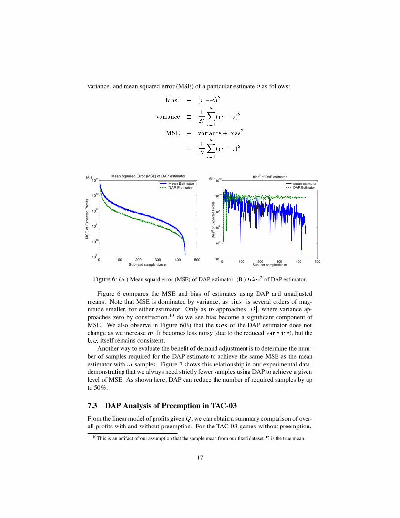
variance, and mean squared error (MSE) of a particular estimate � as follows:

���� � ��� � ���

������ �

�

�����

��� � ����

��� � ������ � ����

�

�

�����

��� � ���

0 100 200 300 400 50010

9

1010

1011

1012

1013

1014

Mean Squared Error (MSE) of DAP estimator

Sub−set sample size m

MS

E o

f Exp

ecte

d P

rofit

s

Mean EstimatorDAP Estimator

(A.)

0 100 200 300 400 50010

2

104

106

108

1010

1012

bias2 of DAP estimator

Sub−set sample size m

Bia

s2 of E

xpec

ted

Pro

fits

Mean EstimatorDAP Estimator

(B.)

Figure 6: (A.) Mean squard error (MSE) of DAP estimator. (B.) ����� of DAP estimator.

Figure 6 compares the MSE and bias of estimates using DAP and unadjustedmeans. Note that MSE is dominated by variance, as ���� is several orders of mag-nitude smaller, for either estimator. Only as � approaches ���, where variance ap-proaches zero by construction,10 do we see bias become a significant component ofMSE. We also observe in Figure 6(B) that the �� of the DAP estimator does notchange as we increase �. It becomes less noisy (due to the reduced ������), but the��� itself remains consistent.

Another way to evaluate the benefit of demand adjustment is to determine the num-ber of samples required for the DAP estimate to achieve the same MSE as the meanestimator with � samples. Figure 7 shows this relationship in our experimental data,demonstrating that we always need strictly fewer samples using DAP to achieve a givenlevel of MSE. As shown here, DAP can reduce the number of required samples by upto 50%.

7.3 DAP Analysis of Preemption in TAC-03

From the linear model of profits given ��, we can obtain a summary comparison of over-all profits with and without preemption. For the TAC-03 games without preemption,

10This is an artifact of our assumption that the sample mean from our fixed dataset� is the true mean.

17

0 100 200 300 400 5000

50

100

150

200

250

300

350

400

450

Number of samples with Mean estimator

Num

ber

of s

ampl

es w

ith D

AP

est

imat

or r

equi

red

for

equi

vale

nt M

SE

Figure 7: Number of samples required by DAP estimator to acheive the same MSE asa given number of samples with the mean estimator.

DAP was –$1.41M. Preemption increased DAP to $5.20M. Thus, we find that on av-erage, Deep Maize’s preemptive strategy improved not only its own profits, but thoseof the other agents as well. These results are corroborated by controlled experimentsdescribed below.

8 Game-TheoreticModel

Although the tournament results presented above are illuminating, it is difficult to sup-port general conclusions due to the many contributing factors and differences amongagents. To isolate the effect of preemption on the key strategic variable (aggressivenessof day-0 procurement), we developed a stylized game-theoretic model, then calibratedit using simulation experiments. Game-theoretic analysis supports conclusions aboutequilibrium behavior of rational agents, providing further evidence that the phenomenaobserved are not merely transient outcomes produced by a particular set of irrationalagents.

We proceed by defining a normal-form game, restricting attention to characteristicstrategies, and estimating payoffs through simulation experiments. We then identify aseries of equilibria, pure and mixed, with respect to various restrictions of the game.Examination of these equilibria and their payoffs confirms that the strategic dynamicobserved in the 2003 TAC/SCM tournament obtains in our more controlled setting aswell.

8.1 Normal-Form Model Structure

As noted at the outset, TAC/SCM defines a six-player game of incomplete and imper-fect information, with an enormous space of available strategies. The game is symmet-

18

ric [Cheng et al., 2004], in that agents have identical action possibilities, and face thesame environmental conditions. In our stylized model, we restrict the agents to threestrategies, differing only in their approach to day-0 procurement. Each strategy is im-plemented as a variant of Deep Maize. By basing the strategies on a particular agent,we clearly cannot capture the diversity of approaches to all aspects of TAC/SCM. Fix-ing much of the behavior, however, enables our focus on the particular issue of strategicprocurement.

In strategy A (aggressive), the agent requests large quantities of components fromevery supplier on day 0. The specific day-0 RFQs issued correspond to aggressive day-0 policies we observed for actual TAC-03/SCM participants. We encoded four of theseas RFQ quantity lists:

1. (4250,5000,5000,2500,1250), based on TacTex [Pardoe and Stone, 2004].

2. (3000,3000,3000,3000,3000), based on UMBCTAC.

3. (4000,3000,8000), based on HarTac [Dong et al., 2004].

4. (1672,1672,1672,1672,1672), and double this for CPU components, based onBotticelli [Benisch et al., 2004].

Strategy A randomly selects among these at the beginning of each game instance.In strategy B (baseline), the agent treats day 0 just like any other day, issuing re-

quests according to its standard policy of serving anticipated demand and maintaininga buffer inventory [Kiekintveld et al., 2004a]. Strategy P (preemptive) is actually DeepMaize as we ran it in the tournament, with preemptive day-0 procurement as describedabove. Each of these strategies follows the standard Deep Maize procurement policyafter day 0.

We consider three versions of this game in our analysis. The first is an unpreemptedsix-player game, where agents are restricted to playing A or B. The second is a five-player game, with the sixth place taken up by a fixed agent playing strategy P. Werefer to this as the single-preemptor game. The third is the full six-player game whereagents are allowed to play any of the three strategies A, B, or P.

Since the three strategies incorporate specified policies for conditioning on privateinformation, we represent the game in normal form. By symmetry there are only sevendistinct profiles for the unpreempted game, corresponding to the number of agentsplaying A, � � � �. There are six distinct profiles for the single-preemptor game,and a total of twenty-eight for the full game (including the thirteen from the morerestricted games). Payoffs for each profile represent the expected profits for playing A,B, or P, respectively, given the other agents, with expectation taken over all stochasticelements of the game environment.

8.2 Simulation Results

To estimate our game’s expected payoff function, we sampled an average of around 30game instances for each strategy profile—834 in total. For each sample, we collectedthe average profits for the As, Bs, and Ps, as well as the demand level, ��. We then

19

used the demand-adjustment method described above to derive DAP for each strategy,which we take as its payoff in that profile.

From this data, we verify that increasing the prevalence of aggressiveness degradesaggregate profits. We show that inserting a single preemptive agent neutralizes theeffect of aggressiveness, diminishing the incentive to implement an aggressive strat-egy, and also ameliorating its negative effects. Moreover, the presence of a preemptortends to improve performance for all agents in profiles containing a preponderance ofagents playing A. We then study the equilibrium behavior of each of the three versionsof the game. From the empirical game models, we derive asymmetric pure-strategyequilibria, as well as symmetric mixed-strategy equilibria, for each of the games.11

Comparison of the features of equilibrium behavior in the respective games confirmsour findings about the effects of strategic preemption.

To test our hypothesis that aggressive strategy has a negative effect on total profits,we regressed total DAP for each profile on the number of aggressive agents in theprofile. For profiles without preemption, the linear relationship was quite strong (� ����� �, �� � ����), with each A in the profile subtracting $20.9M from total profits,on average.

In the single-preemptor game, the effect of number of aggressive agents on averagetotal profits was statistically insignificant, explaining little variance (� � ����, � � ��� �). For unpreempted profiles with four or more aggressive players, agents playingeither strategy would benefit substantially (at least $6.5M in average profits) from oneof the others (either type) switching to play P. Thus, preemption appears to eliminatethe detrimental effect that aggressive agents exert on total profits, and for individualprofits as well compared to profiles with a predominance of strategy A.

We also confirmed that preemption levels the playing field, as the difference in av-erage profits between aggressive and baseline agents was on the order of $10M for theunpreempted profiles, as compared to $1M for the single-preemptor case. Examiningthe variance across agents in each particular game, we observe that average variancefor unpreempted profiles was an order of magnitude larger than that for profiles withpreemption. The variances are tabulated in Table 4.

8.3 Pure Strategy Equilibria

A pure-strategy Nash equilibrium is a strategy profile such that no agent can improve itspayoff by changing strategies, assuming all other agents play according to the profile.We identify pure strategy Nash equilibria for both of the two-strategy games, as wellas the full three-strategy game.

8.3.1 Two-Strategy Games

In a two-strategy (�A,B�) symmetric game, a profile is defined by the number of As.Profile � � � � is a Nash equilibrium if and only if:

11It can be shown that for any� -player two-strategy symmetric game, there must exist at least one equilib-rium in pure strategies, and there also must exist at least one symmetric equilibrium (pure or mixed) [Chenget al., 2004].

20

Profile Variance Baseline Aggressive Preemptive AverageDAP ($M) DAP ($M) DAP ($M) DAP ($M)

AAAAAA 8.37E+15 n/a –12.26 n/a –12.26AAAAAB 8.29E+15 –9.03 –13.58 n/a –12.83AAAABB 1.14E+16 –10.78 –1.47 n/a –4.57AAABBB 9.70E+15 –10.36 9.73 n/a –0.31AABBBB 6.79E+15 –2.47 19.16 n/a 4.74ABBBBB 2.61E+15 –1.83 13.28 n/a 0.69BBBBBB 1.84E+13 8.17 n/a n/a 8.17

PAAAAA 6.38E+14 n/a 6.86 9.98 7.38PAAAAB 6.36E+14 7.23 8.84 10.29 8.82PAAABB 6.50E+14 3.62 5.15 9.04 5.29PAABBB 7.53E+14 6.06 7.34 10.96 7.30PABBBB 1.18E+15 4.19 5.75 11.41 5.65PBBBBB 1.03E+15 6.06 n/a 13.64 7.32

PPAAAA 5.90E+14 n/a 3.67 5.45 4.26PPAAAB 4.24E+14 5.11 4.71 6.69 5.44PPAABB 4.28E+14 4.55 4.70 6.71 5.32PPABBB 4.95E+14 1.74 2.57 4.46 2.79PPBBBB 9.03E+14 4.78 n/a 7.31 5.63

PPPAAA 2.49E+14 n/a 7.41 7.30 7.35PPPAAB 1.75E+14 5.76 5.84 6.32 6.07PPPABB 1.99E+14 10.10 10.14 10.08 10.10PPPBBB 3.51E+14 3.76 n/a 4.30 4.03

PPPPAA 2.33E+14 n/a 2.26 1.50 1.75PPPPAB 2.13E+14 6.98 7.24 6.16 6.48PPPPBB 2.87E+14 5.77 n/a 5.69 5.72

PPPPPA 1.43E+14 n/a 7.74 6.64 6.82PPPPPB 2.04E+14 5.46 n/a 4.39 4.56

PPPPPA 1.19E+14 n/a n/a 4.14 4.14

Table 4: Payoffs by strategy profile. “Variance” refers to the mean variance acrossagents for games with the corresponding profile.

1. the payoff to A in exceeds the payoff to B in � (or � �), and

2. the payoff to B in exceeds that to A in � (or � � ).

We consider the games defined by DAP payoffs, as well as raw average profits. Thefull set of DAP payoffs are provided in Table 4. As we ran our simulations, we observedthat DAP results anticipated those we would obtain from raw averages after collectingmore samples. This is consistent with the experiment described in Section 7.2, in whichwe found that DAP estimates exhibit lower mean-squared-error compared to samplemeans, for a range of subsample sizes going well beyond what we could collect for each

21

profile. Given our relatively small datasets, therefore, we have greatest confidence inthe DAP results. An advantage of the raw averages is that we have associated variancemeasures, enabling statistical hypothesis testing.

Let A denote the profile with no preemption, and agents playing A (the restplaying B). Whether we define payoffs by DAP or raw averages, the unique pure-strategy Nash equilibrium is 4A. That this is an equilibrium for DAP payoffs can beseen by comparing adjacent columns in the bar chart of Figure 8. Arrows indicate foreach column, whether an agent in that profile would prefer to stay with that strategy(arrow head), or switch (arrow tail). Solid black arrows denote statistically significantcomparisons, as discussed below. Profile 4A is the only one with only in-pointingarrows.

Figure 8: DAP payoffs for unpreempted strategy profiles.

Let PA denote the profile with a preemptive agent, and As. In the game withpreemption, we find several pure-strategy Nash equilibria. P4A and P2A are equilibriaunder either payoff measure, and P0A is an equilibrium in the game defined by DAP,but not raw averages. The DAP comparisons are illustrated by Figure 9.

To assess the robustness of these equilibria, we conducted statistical tests. For eachrelevant comparison we performed two-sample t-tests, using average profits, assumingunequal variance. The p-values are presented in Table 5. Whereas some of the com-parisons in the unpreempted game indicate significant differences, for the preemptiveprofiles none of the comparisons are particularly significant. Thus, the equilibria wefound should be considered suspect, or weak equilibria at best. Since payoffs in thepreemptive games have much lower variance, if anything we would expect significantdifferences to show up earlier. This is consistent with our finding above that the pre-emptive agent neutralizes the difference between strategies A and B. In that respect,identifying an equilibrium is less important in this context.

22

Figure 9: DAP payoffs, with preemption.

Regardless of which equilibrium is played, both A and B agents are clearly betteroff in the single-preemptor game. In all its equilibria, all agents earn over $6M profit.In the unpreempted game equilibrium (4A), in contrast, all profits are negative, withthe B agents losing over $10M each.

8.3.2 Full Three-Strategy Game

Our analysis of the two-strategy games confirms our hypothesis that introducing a sin-gle preemptive agent neutralizes the effect of aggressiveness and moves equilibriumplay toward a more profitable space. The success of preemption, however, raises thequestion about whether an incentive to preempt will create a similar mutually destruc-tive competition among preemptors. To check this, we can perform the same kindof equilibrium analysis in the three-player game, where agents are allowed to choosestrategy P. The twenty-eight profiles are arrayed in Figure 10, with arrows indicatingthe transitions between profiles induced by agents switching strategies.

The four pure-strategy Nash equilibria of this game are indicated in bold: PAAAAB,PPBBBB, PPPAAA, and PPPABB. Although the average scores vary across equilibria,in every case the A and B players earn substantial profit, unlike the unpreempted case.Indeed, there exists only one unpreempted profile (2A) from which an A would notdeviate, and no unpreempted profiles where playing B is stable.

We also note that as more agents adopt a preemptive strategy, the difference in per-formance among strategies diminishes. Almost all the comparisons between profileswith preemptive agents are statistically insignificant, as can be seen by the thin arrowsin Figure 10. One way to quantify the indifference between strategies given preemp-tion is to consider the �-Nash equilibria. A profile is �-Nash if no agent can improveits payoff by more than � by deviating from its assigned strategy. In Figure 10, wedisplay for each profile the minimum � that would render it an �-Nash equilibrium. For

23

Comparison P-value

AAAAAA � AAAAAB 0.6595AAAAAB � AAAABB 0.0020AAAABB � AAABBB 0.0246AAABBB� AABBBB 0.5123AABBBB� ABBBBB 0.0001ABBBBB� BBBBBB 0.2879

PAAAAA � PAAAAB 0.7678PAAAAB � PAAABB 0.2294PAAABB � PAABBB 0.4413PAABBB � PABBBB 0.3436PABBBB� PBBBBB 0.3845

Table 5: Statistical significance of profile comparisons.

example, although PPPPPA is not an equilibrium, agents can gain at most $0.34M bydeviating from their assigned strategies. Among the 21 preemptive profiles, 17 of themare �-Nash equilibria at an � of $5.38M or less. In contrast, none of the unpreemptedprofiles are �-equilibria at that level.

8.4 Mixed Strategy Equilibria

Although the pure-strategy equilibria are interesting, we might consider symmetricequilibria more natural, given the symmetry of the game and its lack of identifyingroles [Kreps, 1990]. In order to identify a symmetric equilibrium, we need in generalto consider mixed strategies.

8.4.1 Two-Strategy Games

Let � be the total number of strategies in the profile (in our context, � � � withoutpreemption, and � � � when we include a single fixed preemptive agent). DefineDAP��� � as the DAP of strategy X (A or B) when agents out of � play strat-egy A. If � agents each independently choose whether to play A with probability �(henceforth, “play �”), then the probability that exactly will choose A is given by

����� � �� �

��

���� � ������

Let � ����� denote the DAP of an agent playing A when the remaining agentsplay �:

� ����� ��������

����� �� � �DAP��� � ��

Similarly, we define DAP values for playing B or �, respectively, in the setting where

24

Figure 10: Profiles for the full three-strategy game, with arrows indicating a desireby the associated agent to change its strategy. Statistically significant comparisons areindicated by bold arrows. Values specified for each profile represent the minimum �such that the profile constitutes an �-Nash equilibrium.

others play �:

� ����� ��������

����� �� � �DAP��� ��

� ��� �� � �� ����� � � � ��� ������

We plot these values of playing A, B, or � in response to �, for the two games,in Figure 11. A necessary and sufficient condition for a symmetric mixed-strategyequilibrium is

� ����� � � ������

Therefore, we can identify such equilibria by the points in these figures where thecurves intersect. For the game without preemption, we have a single symmetric mixed-strategy equilibrium, at � � ����. When the preemptive agent is present, we find twosymmetric mixed-strategy equilibria: � � ���� and � � ����.

25

0 0.2 0.4 0.6 0.8 1−1.5

−1

−0.5

0

0.5

1

1.5x 107

V(A,α)V(B,α)V(α,α)

0 0.2 0.4 0.6 0.8 15

5.5

6

6.5

7

7.5x 106

V(A,α)V(B,α)V(α,α)

Figure 11: Response to mixed strategy �, for the unpreempted (left) and single-preemptor (right) games. Note that the payoff scale is an order of magnitude widerin the left graph.

The expected payoff for the equilibrium strategy (equal for A and B, by definition)of the game without preemption is a loss of $9.59M. With a single preemptor, the twoequilibria have expected payoffs of $5.92M and $7.01M, respectively. The preemptiveagent itself also does well, earning profits of $13.3M and $9.99M in the respectiveequilibria.

Although we have no direct way to perform a statistical hypothesis test usingdemand-adjusted values, a conservative option is to compare the mean DAP scoresusing the variance of the raw averages. In this instance, DAP for the two preemptiveequilibria exceed that of the non-preemptive equilibrium at p-values less than 0.0001.

Inspection of Figure 11 confirms our prior finding that preemption reduces the dif-ference between A and B strategies. One way to quantify this is to identify an �� foreach game such that any mixed strategy is a symmetric �-Nash equilibrium at � � ��.In our context, �� is therefore the maximum payoff difference between playing thebest-response strategy, and playing �:

�� � �

��

���� �� ������ � ��� ��

��

For games without preemption, �� is $10.6M. With preemption, �� is only $0.97M.This provides a bound on how much it can matter to make the right choice about ag-gressiveness, given a symmetric set of other agents.

8.4.2 Full Three-Strategy Game

We were also able to derive a symmetric mixed-strategy equilibrium for the full three-strategy game, using replicator dynamics [Schuster and Sigmund, 1983]. In equilib-rium, agents play A with probability 0.23, B with probability 0.19, and P with 0.58.The expected payoff for this mixed strategy is $5.78M. This is not quite as good asthe environment allowing only a single preemptor, but of course much better than theunpreempted situation.

26

9 Procurement Strategy in TAC-04 and Beyond

Based on the 2003 experience, the TAC/SCM game designers revised the game rulesfor TAC-04, with the primary intent of reducing the attraction of aggressive day-0procurement. The modified supplier pricing rule imposed premiums for large orders,and the new storage fee added a proportional cost for holding component inventory.Although these may have had some deterrent effect, they were apparently not sufficientto prevent aggressive day-0 procurement in the 2004 tournament. They did, however,effectively rule out preemptive remedies of the sort that Deep Maize provided in TAC-03. In consequence, the tournament games exhibited major procurement imbalances,and surprisingly volatile profits given the much steadier demand process introduced for2004. Further analysis will be required to characterize agents’ procurement strategiesin TAC-04, and explain the full strategic implication of the rule changes.

In order to remove day-0 procurement as an overriding issue once and for all, thedesigners for TAC-05 [Collins et al., 2004] are completely overhauling the method bywhich suppliers allocate offers. We look forward to investigating the other strategictrading issues that will inevitably come to the fore in the 2005 TAC/SCM game.

10 Conclusion

The TAC supply-chain game presented automated trading agents (and their design-ers) with a challenging strategic problem. Embedded within a highly-dimensionalstochastic environment was a pivotal strategic decision about initial procurement ofcomponents. Our reading of the game rules and observation of the preliminary roundssuggested to us that the entrant field was headed toward a self-destructive, mutuallyunprofitable equilibrium of chronic oversupply. Our agent, Deep Maize, introduceda preemptive strategy designed to neutralize aggressive procurement. It worked. Notonly did preemption improve Deep Maize’s profitability, it improved profitability forthe whole field. Whereas it is perhaps counterintuitive that actions designed to preventothers from achieving their goals actually helps them, strategic analysis explains howthat can be the case.

Investigating strategic behavior in the context of a research competition has severaldistinct advantages. First, the game is designed by someone other than the investigator,avoiding the kinds of bias that often doom research projects to success. Second, theentry pool is uncontrolled, and so we may encounter unanticipated behavior of individ-ual agents and aggregates. Third, the games are complex, avoiding many of the biasesfollowing from the need to preserve analytical or computational tractability. Fourth,the environment model is precisely specified and repeatable, thus subject to controlledexperimentation. We have exploited all of these features in our study, in the processdeveloping a repertoire of methods for empirical game-theoretic analysis, which weexpect to prove useful for a range of problems.

There is no doubt that this form of study also has several limitations, for examplein justifying generalizations beyond the particular environment studied. Nevertheless,we believe that the methods developed here provide a useful complement to the kindsof (a priori) stylized modeling most often pursued in game-theoretic analysis, and to

27

the non-strategic analyses typically applied to simulation environments.

Acknowledgments

Thanks to the TAC/SCM organizers and participants, and to anonymous reviewers forconstructive comments. At the University of Michigan, Deep Maize was designedand implemented with the additional help of Shih-Fen Cheng, Thede Loder, KevinO’Malley, and Matthew Rudary. Daniel Reeves assisted our equilibrium analyses. Thisresearch was supported in part by NSF grant IIS-0205435.

References

Olivier Armantier, Jean-Pierre Florens, and Jean-Francois Richard. Empirical game-theoretic models: Constrained equilibrium and simulations. Technical report, StateUniversity of New York at Stonybrook, 2000.

Raghu Arunachalam, Joakim Eriksson, Niclas Finne, Sverker Janson, and NormanSadeh. The TAC supply chain management game. Technical report, Swedish In-stitute of Computer Science, 2003. Draft Version 0.62.

Raghu Arunachalam and Norman M. Sadeh. The supply chain trading agent competi-tion. Electronic Commerce Research and Applications, to appear.

Michael Benisch, Amy Greenwald, Ioanna Grypari, Roger Lederman, Victor Narodit-skiy, and Michael Tschantz. Botticelli: A supply chain management agent designedto optimize under uncertainty. SIGecom Exchanges, 4(3):29–37, 2004.

Shih-Fen Cheng, Daniel M. Reeves, Yevgeniy Vorobeychik, and Michael P. Well-man. Notes on equilibria in symmetric games. In AAMAS-04 Workshop on Game-Theoretic and Decision-Theoretic Agents, New York, 2004.

John Collins, Raghu Arunachalam, Norman Sadeh, Joakim Eriksson, Niclas Finne,and Sverker Janson. The supply chain management game for the 2005 trading agentcompetition. Technical report, Carnegie Mellon University, 2004.

Erik Dahlgren. PackaTAC: A conservative trading agent. Master’s thesis, Lund Uni-versity, 2003.

Rui Dong, Terry Tai, Wilfred Yeung, and David C. Parkes. HarTAC: The Harvard TACSCM ’03 agent. In AAMAS-04 Workshop on Trading Agent Design and Analysis,New York, 2004.

Richard O. Duda, Peter E. Hart, and David G. Stork. Pattern Classification. Wiley-Interscience, second edition, 2000.

Drew Fudenberg and Jean Tirole. Game Theory. MIT Press, 1991.

Herbert Gintis. Game Theory Evolving. Princeton University Press, 2000.

28

Philipp W. Keller, Felix-Olivier Duguay, and Doina Precup. RedAgent: Winner ofTAC SCM 2003. SIGecom Exchanges, 4(3):1–8, 2004.

Jeffrey O. Kephart and Amy R. Greenwald. Shopbot economics. Autonomous Agentsand Multiagent Systems, 5:255–287, 2002.

Jeffrey O. Kephart, James E. Hanson, and Jakka Sairamesh. Price and niche wars in afree-market economy of software agents. Artificial Life, 4:1–23, 1998.

Wolfgang Ketter, Elena Kryzhnyaya, Steven Damer, Colin McMillen, AmrudinAgovic, John Collins, and Maria Gini. Design and analysis of the MinneTAC-03supply-chain trading agent. Technical Report 04-016, University of Minnesota, Deptof Computer Science and Engineering, 2004.

Christopher Kiekintveld, Michael P. Wellman, Satinder Singh, Joshua Estelle, Yev-geniy Vorobeychik, Vishal Soni, and Matthew Rudary. Distributed feedback controlfor decision making on supply chains. In Fourteenth International Conference onAutomated Planning and Scheduling, pages 384–392, Whistler, BC, 2004a.

Christopher Kiekintveld, Michael P. Wellman, Satinder Singh, and Vishal Soni. Value-driven procurement in the TAC supply chain game. SIGecom Exchanges, 4(3):9–18,2004b.

David M. Kreps. Game Theory and Economic Modelling. Oxford University Press,1990.

Pierre L’Ecuyer. Efficiency improvement and variance reduction. In Twenty-SixthWinter Simulation Conference, pages 122–132, Orlando, FL, 1994.

David Pardoe and Peter Stone. TacTex-03: A supply chain management agent. SIGe-com Exchanges, 4(3):19–28, 2004.

Daniel M. Reeves, Michael P. Wellman, Jeffrey K. MacKie-Mason, and Anna Osepa-yshvili. Exploring bidding strategies for market-based scheduling. Decision SupportSystems, to appear.

Sheldon M. Ross. Simulation. Academic Press, third edition, 2002.

Norman Sadeh, Raghu Arunachalam, Joakim Eriksson, Niclas Finne, and Sverker Jan-son. TAC-03: A supply-chain trading competition. AI Magazine, 24(1):92–94, 2003.

P. Schuster and K. Sigmund. Replicator dynamics. Journal of Theoretical Biology,100:533–538, 1983.

Peter Stone. Multiagent competitions and research: Lessons from RoboCup and TAC.In Sixth RoboCup International Symposium, Fukuoka, Japan, 2002.

William E. Walsh, Rajarshi Das, Gerald Tesauro, and Jeffrey O. Kephart. Analyzingcomplex strategic interactions in multi-agent systems. In AAAI-02 Workshop onGame-Theoretic and Decision-Theoretic Agents, Edmonton, 2002.

29

William E. Walsh, David Parkes, and Rajarshi Das. Choosing samples to computeheuristic-strategy Nash equilibrium. In AAMAS-03 Workshop on Agent-MediatedElectronic Commerce, Melbourne, 2003.

Michael P. Wellman, Shih-Fen Cheng, Daniel M. Reeves, and Kevin M. Lochner. Trad-ing agents competing: Performance, progress, and market effectiveness. IEEE Intel-ligent Systems, 18(6):48–53, 2003.

Dongmo Zhang, Kanghua Zhao, Chia-Ming Liang, Gonelur Begum Huq, and Tze-HawHuang. Strategic trading agents via market modelling. SIGecom Exchanges, 4(3):46–55, 2004.

30