Stock Return and Financial Media Coverage Bias1

Shengle Lin shengle_lin@haas.berkeley.edu

Haas School of Business, University of California, Berkeley

545 Student Service Building, #1900

Berkeley, CA 94720

October 2011

                                                            I thank Dow Jones News Service for providing the news data, Paul Tetlock for offering consolidated media coverage data, Terrance Odean for excellent critiques and Brad Barber for insightful comments. The author thank International Foundation for Experimental Economics, Searle Foundation Trust and Interdisciplinary Center for Economic Science for financial support. Correspondences to: shengle_lin@haas.berkeley.edu

Stock Return and Financial Media Coverage Bias

Abstract: Using news publications from Dow Jones News Services and the Wall Street Journal from 1979

to 2007, I test the relationship between stock returns and changes in media coverage. When stocks are

sorted on past 12-month cumulative abnormal returns, past winners receive higher abnormal coverage in

the current month than past losers. When the return sorting window is shortened to four weeks, stocks in

the both extreme quintiles receive higher abnormal coverage within the four weeks. However, in the

following weeks, abnormal coverage for the top winners remains above average, while that of the bottom

losers drops to levels below average stocks. Media coverage exhibits a long-run bias toward past winners

and a short-run bias toward high contemporaneous absolute returns. I examine three types of potential

intermediating factors: firm’s information supply, analyst coverage and media selection. I find that: (1)

press releases from firms only have weak impact on media coverage, suggesting that firms’ investor

relation activities can hardly control media coverage; (2) past winners have increased numbers of analysts

following the stocks and stories reported on high-analyst-coverage stocks are longer, indicating that

analyst coverage is an important mediating factor; (3) around earnings announcement, the media give

stocks with extreme post announcement return both more stories and higher percentage of stories with

“hot” news label, suggesting that the media prefer to write stories on extraordinary events. Our

investigation suggests that the long-run coverage bias is likely to result from accessibility of firm-specific

information and the short-run coverage bias is likely to draw from the media selection.

Keyword: Media Coverage, Stock Return, Press Release, Earnings, Coverage Bias, Stale News

“It’s always a buying time, never a selling time.” – Gerald Celente, August 2011, criticized the financial

media in persuading investors to buy stocks in all economic conditions.

1. Introduction

Recent research on the relationship between financial news and stock returns suggests that media

coverage can be manipulated by firms or the investor relationship (IR) vendors that are hired by firms.

Gurun (2010) finds that firms, with the help of a media expert on the board of directors, can have their

bad news reported with 18% fewer negative words, and have their good news receive 20% more media

coverage. Similarly, Solomon (2011) finds that IR firms help their clients generate more media coverage

of positive press releases and less of negative releases. Others have documented a local media bias toward

local firms (Gurun and Butler, 2010). These studies suggest that media coverage is influenced by firms

themselves and that firms would like to boost the coverage on their good performance. I refer to this

tendency of firms to promote their news as supply preference.

Fewer studies have addressed any distortion from the media side, that is, whether the media itself would

exhibit a preference for a certain type of news in the absence of conflicting interests noted in Gurun and

Butler (2010). Like any type of media, financial media must decide what news to be covered in order to

better compete for the attention of investors. Hamilton (2004) argues that editors must select content to

appeal to the subscribers in order to maximize subscriptions. In media coverage on celebrities, for

example, negativity bias clearly exists. It reflects that the media caters to the taste of the public rather than

that these negative stories are more readily available. This suggests that the media’s preference overrules

the supply preferences. Solomon and Soltes (2011) show that print newspaper covers more on

contemporaneous extreme earning surprises2. They argue that media caters to the sensationalism sought

by readers.

What kind of stories would financial media like to carry, holding other factors fixed? Sensationalism

cannot be the only objective of financial media. Tetlock (2010a) argues that financial media serves an

information intermediary role in resolving information asymmetry. It is reasonable to assume that readers

do not read the Wall Street Journal or tune into Mad Money just to get shocked. In most likelihood,

subscribers hope to identify investment opportunities from the media.

If the goal of readers is to seek investment information, then the media would have to steer the focus

toward the needs of investors. For example, a key characteristic of investor behavior is chasing past

returns. Barber and Odean (2008) document that retail investors tend to buy stocks with strong past

returns, a pattern that is consistent with representative bias. Grinblatt, Titman and Wermers (1995) find

that 77 percent of mutual funds are “momentum investors,” buying stocks that were past winners. If

average investors chase past winners, they would prefer the media to offer more information on these

winning stocks. The preferences of the media and the subscribers rarely have been studied. I refer to this

preference, if it exists, as demand preference.

This study serves to answer two questions: (1) What is the relationship between stock returns and follow-

up media coverage? Fang and Peress (2010) and Tetlock (2010b) both examine the impact of media

coverage on future stock returns. This paper takes on an opposite perspective and studies how historic

return affects future media coverage. (2) If there is a media coverage slant, where might it originate?

Using comprehensive data on news publications from the Dow Jones News Service and the Wall Street

Journal from 1979 to 2007, I measure media coverage on a stock as the number of stories reported on a

stock in a period (day, week, or month). I examine how media coverage changes in response to stocks’

past and current performance. Change in media coverage is measured as the difference between stories in

                                                            2 Solomon and Soltes (2011) find that print newspapers cover more heavily on extreme negative earnings report, but the tilt toward negativity is not found among newswire.

the current month and the moving average of stories prior to the return sorting window. The difference

also can be seen as abnormal coverage. When sorted on past 12-month cumulative abnormal returns

(CAR), stocks with the highest return receive more abnormal coverage in the current month, and the

coverage sustains at elevated levels in the following months, too; stocks with the lowest return do not

experience any increase in coverage, and their coverage subsequently stays at lower-than-average levels.

The pattern is robust after controlling for firms’ market capitalization, contemporaneous return, analyst

coverage, price-earnings ratio and industry fixed effect. The bias also exists when the historic return sorts

are limited to the past six months or three months.

When I shorten the return sorting window to four weeks, stocks with extreme returns, both positive and

negative, receive the highest abnormal coverage. This suggests that media coverage is higher for both the

best performing stocks and the worst performing stocks in the short-run. The short-run bias toward

extreme returns is consistent with the findings of Solomon and Soltes (2011). However, in the weeks

following the sorting weeks, coverage on high return stocks remains above average, while coverage on

low return stocks drops below average (even though the return differences across the two groups in post-

sorting weeks are similar). Again, the shift in media coverage indicates a coverage bias toward high past

performance.

To examine where the cross-section media coverage differences might be originated, I can examine three

types of potential factors: firms’ supply of information, analyst coverage and media’ reporting preference.

The first test involves controlling for the number of press releases issued by the firms both in the return

sorting period and in the current month. Dow Jones News Service provides a tag, called “press release,”

on news that is a press release from a firm. The null hypothesis is that if firms with more press releases

can influence their media coverage, stocks with the same amount of press releases should experience the

same amount of coverage. The data show that news coverage bias toward high historic return is robust

after controlling for press release. Past press releases do not have an impact on future media coverage,

though contemporaneous press releases are correlated with abnormal coverage. The impact of press

releases on media coverage is likely to be short-lived and do not contribute to long-run coverage bias.

The second test looks at the influence of analyst coverage. I find that stocks with more analysts following

receive more coverage as well as more detailed stories (longer in length).

The third test investigates a set of earnings announcement events. Following earnings announcement, the

media quickly cover the event, with the majority of reports appearing within hours of announcement. I

find that media gives more earnings-specific reports as well as high percentage of “hot news” labels to

extreme returns.

I provide strong evidences that media coverage is biased and the robust findings on media coverage bias

are important to studies on media effect and attention3.

The rest of the paper is structured as follows: Section 2 presents the data, methodology, and main results;

Section 3 evaluates the relative impact of news supply bias and media demand bias; Section 4 compares

the results with that of other studies; and Section VI concludes.

2. Data, Methodology and Main Results

2.1 Data Source

The news data source used in this study is the same as in Tetlock (2010b), which uses the Dow Jones (DJ)

news archive containing all DJ News Service and the Wall Street Journal (WSJ) stories from 1979 to

2007. DJ breaks each news story into multiple fragment messages that are sent out at the earliest time

when each becomes available. DJ newswire is the most widely circulated financial news in the United

States for institutional investors has the most comprehensive coverage. The DJ firm code identifier at the

                                                            3 Researchers have shown that media coverage is directly related to investor attention and trading (Barber and Odean, 2008; Engelberg and Parsons, 2009).

beginning of each newswire is used to check whether a story mentions a publicly traded US firm4. When

a story mentions multiple ticker codes, I keep only the stories with three ticker codes or fewer. Each news

story is matched to a particular date using a 4 p.m. to 4 p.m. market close-to-close rule. Refer to Tetlock

(2010b) for a more comprehensive view.

I limit the subset of news to stories with at least 30 words5 in length. The analysis here is limited to stocks

with the following criteria:

(1) Traded in NYSE, AMEX or NASDAQ;

(2) With a share code 10 or 11, which refers to common stocks;

(3) Average monthly stock price must be greater than $5 in all active months;

(4) Average monthly market capitalization must be greater than $10 million in all active months;

(5) Average monthly traded shares must be greater than 50,000 in all active months;

(6) Stocks must have at least two years of active trading record during the sample period.

This leaves a sample of 8314 stocks, and a total number of 3,175,921 news stories (excluding 557,013

press releases). The average number of stories per stock per month is 2.65. Table 1 provides the basic

summaries on the news coverage. The number of stocks in the sub-period 2000-2007 decreases slightly

from the previous sub-period 1900-1999, because a lot of stocks were delisted or merged in the burst of

the Internet bubble.

I obtain daily and monthly stock returns, stock price and common shares outstanding from CRSP,

earnings information from Compustat, and analyst coverage from I/B/E/S. The stock’s market

capitalization is computed as the share price times the common shares outstanding at a specific time. P/E

                                                            4 Tetlock (2010b) indicate that prior to November 1996, stories without any firm codes sometimes mention US firms—i.e., the DJ firm codes contain measurement error. More seriously, DJ may back-fill firm codes prior to November 1996 in a systematic fashion that introduces survivorship bias in the data. This survivorship bias does not seem to affect stories after November 1996. Between 95% and 99% of sample firms have news coverage in each year after 1996. 5 Tetlock (2010b) cuts off at 50 words to allow for textual mining. Since this study does not address the content of news, the cutoff is set to 30 words instead. 

ratio is computed as the price at the end of fiscal year-end month divided by the earnings per share

(diluted and excluding extraordinary items) for the fiscal year.

Table 1: News Stories Summary Statistics The Dow Jones Newswire covers a date range of 1979 to 2007. The table breaks the sample into 3 periods, 1979-1989, 1990-1999 and 2000-2007. The total number of stories, the number of stocks covered, average number of stories per stock per month, and the average market capitalization of covered stocks are reported

1979-1989 1990-1999 2000-2007 All Years

#Total Stories 176,483 1,728,487 2,853,608 4,758,578 # Stocks Covered 1,713 6,973 6,554 9,107

Average Market Cap 0.8×109 1.5×109 3.4×109 2.1×109

# Stories/stock

mean 103.03 247.88 435.4 312.24 min 1 1 1 1 p25 24 56 53 49 p50 58 117 186 124 p75 111 227 415 287 max 2,771 20,007 27,500 27,500

# Stories/stock/month

mean 2.35 7.46 9.13 7.68

min 1 1 1 1

p25 1 2 2 2

p50 1 4 4 3

p75 3 7 9 7

max 109 820 727 820

2.2 Monthly Abnormal News Sorted on Past 12-month Cumulative Abnormal Returns (CAR)

The major question is how the past performance of a stock would affect its future news coverage. The

investigation starts with monthly news coverage.

In each month of 1981-2007 (month 0), I sort stocks into 10 return bins based upon their past 12-month

Cumulative Abnormal Returns (CAR, from month -12 to month -1). Abnormal return is computed as the

excess return over the equally-weighted market return (NASDAQ/NYSE/AMEX combined). Monthly

abnormal returns are compounded to arrive at the 12-month CAR. Bin 1 has the lowest CAR, and bin 10

has the highest CAR. I examine how media coverage changes in response to the past 12-month return

performance and construct an abnormal coverage variable, abnews:

11,,11,12 , ]13,24[,,, jnewsaveragenewsabnews ttijtijti

The control period is months [-24, -13] and is fixed relative to month 0. The return sorting period is

months [-12,-1]. The observation period for subsequent news coverage is months [0,11].

I use the change in coverage and abnormal coverage, instead of levels of coverage, for two reasons: (1)

level of stories is non-stationary and tends to grow over years, thus making it improper for time-series

comparisons; (2) using the historic average as a control can remove much of stock-specific fixed effects,

many of which are unobservable heterogeneities.

I use the moving average of stories in months [-24, -13] as a denominator, instead of using the average in

months [-12,-1], to avoid potential correlation with the sorting variable. This is important for isolating the

impact of CAR in months [-12, -1] because it is not known yet how the 12-month CAR would interact

with the news coverage in the same period. The moving average in months [-24,-13] gives a fixed anchor

that is not influenced by the return in month [-12,-1].

Figure 1 Panel A plots the monthly abnormal news for each of 10 return bins from month -12 to month

11, spanning two years. At month 0, stocks are grouped into 10 bins based upon their past 12-month

CAR. The abnormal news for an individual stock is obtained by subtracting the average news in months

[-24,-13] from the news in the month 0. Next, the average of abnormal news for all stocks in a bin at

month 0 is computed. Finally, I arrive at the time-series average of each of the 10 bins. The time series

starts from 1981, two years after the beginning of available date, and ends at 2007. Each bin time series

covers 324 months.

A potential concern is the survivorship bias. When stocks are included in the sorting period [-12,-1], they

may get delisted in the months [0,11]. Since I sort on returns in the past and examine news coverage in

the future, it is inevitable that I come across stocks that are delisted in the subsequent period but still

receive news coverage. In particular, stocks with extremely low past returns are more likely to be delisted

in the following months. Delisted stocks may no longer receive news coverage, since their ticker codes

will no longer be mentioned in the newswires. This would bias the coverage in the low return bin

downward. To avoid this downward bias, I include the stories in months [0, 11] only when a stock is

actively traded in this period.

Panel A shows the evolution of news coverage in both the sorting period [-12, -1] and the subsequent

period [0, 11]. In Figure 1 Panel A, the short-dash blue line in the middle delineates the average

abnormal news for all stocks. The upward trend shows that the average stock experiences more news

reports over the time (each month has the same denominator). The slope for the average trend is constant,

suggesting that abnormal news is relatively stationary over time. As can been seen, the best

outperforming bin received increased coverage during the sorting period and the coverage sustains at the

highest levels in the subsequent months. The coverage on the worst performing bin experiences slightly

above-average growth in month -11, but the growth ceases afterwards and falls to the bottom after month

-7. The distance in coverage between the worst performing bin and the average stocks widens over time.

In the post-sorting months [0,11], the abnormal coverage across bins exhibits an ordering perfectly

coinciding with the respective 12-month CARs.

Panel B reports the monthly abnormal returns for each bin. In the sorting period [-12, -1], the returns

spread across bins are large (by construct). In the subsequent period [0, 11], the spread is small. Stocks

experiencing high (low) past returns continue to outperform (underperform), but the continuation is

reverted after month 66. This suggests that the past 12-month CARs are more likely to be the main drivers

for the subsequent abnormal coverage difference, rather than the returns in months [0, 11]. It should be

noted that past winners do not have to outperform in every single month. The high abnormal returns in

each month of the sorting period reflect the average of all stocks in the bin.

                                                            6 Fang and Peress (2010) argue that current coverage can drive future returns. Our results suggest that past returns are correlated with current coverage. Given that returns are generally correlated over time horizons, our results would suggest a careful re-examination of their argument. Future returns could have been affected by past returns, too.

Figure1. Stock Returns and Abnormal Monthly News: 1981-2007 Panel A:

Panel B:  

To be more precise, the sorting needs to be controlled for contemporaneous returns. In addition, Solomon

and Soltes (2011) pointed out that large firms tend to receive much higher media coverage. Table 2

investigates the effect of the past 12-month CAR on the current month media coverage whilewith the

controlling for market capitalization and contemporaneous return in the current month.

In Table 2, I test whether past winners receive higher abnormal news in the current month than past losers

do, conditioned on market capitalization and contemporaneous returns. Stocks first are split into five

market cap bins based upon their market cap in lagged 13 months. The reason to use a lagged 13-month

cap is to avoid the interference between present market cap and past 12-month CAR. If I pick the market

cap at the end of month -1, it would be highly correlated with the past 12-month CAR. In this case, the

larger firms will automatically have higher past returns and the effect of past returns will be diluted.

Each size bin is further split into five contemporaneous return sub-bins based upon their abnormal returns

in the current month. In each of the 25 sub-bins, stocks are split into five past return quintiles based upon

their past 12-month CAR. This sorting scheme ensures the number of stocks in each bin are equalized to

the largest extent. Panel A reports on abnormal news in the current month. The results show that for

stocks with the same cap quintile and contemporaneous return quintile, quintile 5 of the 12-month CAR

consistently has higher abnormal news coverage than quintile 1 of the 12-month CAR. For each size-by-

contemporaneous-return pair, 324 months of differences are obtained. To test the statistical difference

against the null that the difference is zero, I compute Newey-West standard errors with six lags to arrive

at t-statistics. The t-statistics are significant at 0.01 level in 23 out of 25 comparisons. In cap quintile 1-4,

the difference between the low 12-month CAR quintile and the high 12-month CAR quintile is highly

significant. In cap quintile 5, the adjusted standard errors go up, driving down the t-statistics. Yet, the

difference remains positive.

Panel B is a complementary table reporting the average past 12-month CAR for each of 125 bins.

Smaller firms on average haves higher past CAR. The past winners outperform the past losers by

economically large amounts.

An interesting fact is that the contemporaneous monthly return has a U-shaped effect on news coverage.

The lowest current month return bin does not receive the least amount of abnormal coverage. Instead, in

all of the size quintiles, stocks in the lowest current abnormal return quintile and those in the highest

quintiles have higher abnormal coverage than those in the middle quintiles. This suggests that, in the short

run, the return-coverage relationship is U-shaped. Section 2.3 will verify this specifically with a shortened

return sorting window.

Low

-12

34

Hig

h-5

Q5-

Q1

Low

-12

34

Hig

h-5

Q5-

Q1

Low

-10.

073

0.05

90.

080

0.11

90.

292

0.21

90.

040*

**L

ow-1

-0.5

63-0

.284

-0.0

510.

280

1.51

52.

078

2-0

.026

0.01

30.

019

0.07

30.

136

0.16

20.

033*

**2

-0.4

47-0

.194

-0.0

130.

219

1.11

11.

558

30.

008

0.02

40.

043

0.07

50.

146

0.13

80.

027*

**3

-0.4

26-0

.172

-0.0

050.

200

0.97

41.

399

40.

022

0.03

30.

077

0.11

00.

196

0.17

40.

035*

**4

-0.4

42-0

.181

-0.0

010.

231

1.09

71.

539

Hig

h-5

0.18

40.

213

0.23

40.

254

0.45

60.

272

0.04

5***

Hig

h-5

-0.5

37-0

.239

0.00

00.

322

1.49

82.

034

Low

-10.

088

0.14

10.

144

0.22

30.

479

0.39

10.

070*

**L

ow-1

-0.5

75-0

.323

-0.1

190.

144

0.93

71.

512

20.

021

0.03

50.

077

0.08

50.

176

0.15

50.

040*

**2

-0.4

59-0

.215

-0.0

510.

144

0.71

91.

178

30.

004

0.02

90.

067

0.13

60.

164

0.15

90.

035*

**3

-0.4

26-0

.184

-0.0

330.

142

0.65

61.

082

40.

054

0.07

00.

097

0.15

60.

256

0.20

20.

036*

**4

-0.4

38-0

.194

-0.0

290.

160

0.73

71.

175

Hig

h-5

0.20

20.

256

0.25

60.

328

0.55

50.

353

0.07

2***

Hig

h-5

-0.5

35-0

.262

-0.0

520.

204

0.95

61.

490

Low

-10.

182

0.14

20.

214

0.27

80.

618

0.43

60.

095*

**L

ow-1

-0.5

67-0

.316

-0.1

260.

112

0.73

91.

306

2-0

.060

0.03

40.

094

0.08

30.

310

0.37

00.

065*

**2

-0.4

50-0

.208

-0.0

530.

121

0.59

91.

049

3-0

.041

0.03

60.

079

0.12

10.

276

0.31

70.

046*

**3

-0.4

15-0

.178

-0.0

350.

122

0.55

50.

970

4-0

.014

0.07

60.

137

0.17

80.

303

0.31

70.

056*

**4

-0.4

26-0

.186

-0.0

330.

138

0.61

71.

043

Hig

h-5

0.22

80.

289

0.34

80.

418

0.72

40.

496

0.09

2***

Hig

h-5

-0.5

20-0

.257

-0.0

680.

156

0.76

21.

282

Low

-10.

402

0.36

30.

370

0.45

30.

858

0.45

60.

145*

**L

ow-1

-0.5

16-0

.265

-0.0

960.

093

0.58

21.

098

20.

009

0.07

80.

119

0.21

30.

480

0.47

20.

078*

**2

-0.3

95-0

.171

-0.0

390.

106

0.48

00.

875

30.

007

0.07

50.

104

0.16

20.

448

0.44

10.

088*

**3

-0.3

69-0

.151

-0.0

300.

100

0.45

00.

820

40.

080

0.09

60.

167

0.28

70.

558

0.47

80.

090*

**4

-0.3

82-0

.162

-0.0

320.

107

0.47

90.

860

Hig

h-5

0.44

60.

456

0.52

70.

648

1.10

00.

654

0.15

4***

Hig

h-5

-0.4

73-0

.227

-0.0

640.

120

0.60

41.

077

Low

-11.

707

1.68

41.

491

1.30

52.

533

0.82

60.

529

Low

-1-0

.412

-0.2

01-0

.069

0.07

50.

434

0.84

62

0.81

70.

410

0.68

01.

089

1.63

80.

821

0.46

3*2

-0.3

20-0

.136

-0.0

310.

080

0.35

60.

676

30.

710

0.49

60.

579

0.93

01.

529

0.81

80.

478*

3-0

.304

-0.1

28-0

.028

0.08

30.

344

0.64

84

0.76

60.

651

0.65

11.

082

2.09

11.

326

0.51

9**

4-0

.311

-0.1

33-0

.029

0.08

30.

357

0.66

9H

igh-

51.

552

1.35

41.

610

1.66

73.

303

1.75

10.

605*

**H

igh-

5-0

.389

-0.1

81-0

.054

0.08

70.

448

0.83

7

33

In e

ach

mon

th f

rom

198

1 to

200

7, (

1) s

tock

s ar

e fir

st s

orte

d in

to 5

siz

e bi

ns b

ased

upo

n th

eir

mar

ket c

apita

lizat

ion

13 m

onth

s ag

o, r

ight

bef

ore

the

sort

ing

perio

d of

lagg

ed 1

2 m

onth

s; (

2) in

eac

h si

ze b

in,

the

stoc

ks a

re f

urth

er s

plit

into

5 b

ins

base

d up

on th

eir

CA

R in

the

obse

rvat

ion

mon

th; (

3) in

eac

h of

5 b

y 5

bins

, sto

cks

are

split

into

5 q

uint

iles

base

d up

on th

eir

past

12-

mon

th C

AR

(m

onth

-12

to -

1). I

n ea

ch m

onth

, sto

cks

are

split

into

125

bin

s. F

or e

ach

stoc

k in

a b

in, o

btai

n th

e ab

norm

al n

ews,

by

subt

ract

ing

the

aver

age

mon

thly

sto

ries

for

a st

ock

betw

een

mon

th -

24 a

nd -

13, f

rom

the

mon

thly

sto

ries

for

the

stoc

k in

a o

bser

vatio

n m

onth

. For

eac

h bi

n-m

onth

pai

r, th

e m

ean

acro

ss th

e in

clud

ed s

tock

s is

com

pute

d. T

hus,

a ti

me

serie

s (3

24 m

onth

s) o

f m

eans

is o

btai

ned

for

each

bin

. D

iffer

ence

s ar

e co

mpu

ted

for

the

high

est 1

2-m

onth

CA

R q

uint

al a

nd th

e lo

wes

t 12-

mon

th C

AR

qui

ntile

, arr

ivin

g at

a ti

me

serie

s of

324

mon

ths

diff

eren

ces

for

each

bin

. t-

stat

istic

s ar

e pr

ovid

ed f

or th

e di

ffer

ence

s us

ing

New

ey-W

est s

tand

ard

erro

rs w

ith 6

lags

. The

abn

orm

al c

over

age

is r

epor

ted

in P

anel

A. P

anel

B r

epor

ts th

e av

erag

e12-

mon

th C

AR

for

eac

h of

125

bin

s.**

* 0.

01 *

*0.0

5 *

0.10

44

Lar

ge-5

Lar

ge-5

Qui

ntile

on

past

12-

Mon

th C

AR

smal

l-1sm

all-1

22

Mar

ket

Cap

AR

in

Mon

th 0

Qui

ntile

on

past

12-

Mon

th C

AR

N.W

.St

d. E

rr.

Mar

ket

Cap

AR

in

Mon

th 0

Tab

le 2

: A

bnor

mal

New

s s

orte

d on

Pas

t 12

-Mon

th C

AR

, Con

trol

ling

for

Mar

ket

CA

P a

nd C

onte

mpo

rane

ous

Ret

urn:

198

1-20

07

Pan

el A

: Abn

orm

al N

ews

Pan

el B

: P

ast 1

2-M

onth

CA

R

2.3 Weekly Abnormal News sorted on 4-week CAR

Section 2.2 examines the effect of 12-month CAR on subsequent coverage. Table 2 suggests that past 12-

month CAR have a linear impact on current month coverage, but the contemporaneous return seems to

have a U-shaped impact on current month coverage. It seems that the short-run return effect would be

different from the long-run return effect. To examine the contemporaneous return effect closely, I now

shorten the return sorting period into about a month. To capture more details within a month, I focus on

news coverage by week.

In Figure 2, I examine media coverage response to short-run return shocks. At each week, i.e. week 0,

stocks are sorted into 10 bins based upon the past four-week CAR. The weekly abnormal news is reported

for weeks [-4, 11]. The weekly abnormal news is defined as weekly news minus the 52-week moving

average prior to the sorting period:

11,,3,4 , ]5,56[,,, jnewsweeklyaveragenewsweeklyabnewsweekly ttijtijti

The control period is weeks [-56, -5] and is fixed relative to week 0. The return sorting period is weeks [-

4,-1]. The observation period for subsequent news coverage is weeks [0,11].

Figure 2 Panel A plots the weekly abnormal news from week -4 to week 11 for each bin. Panel B plots the

weekly abnormal returns for each bin. In Panel A, the blue short-dash line delineates the abnormal news

coverage for all stocks. The slope of line is constant, suggesting news growth is relatively stationary. In

the four-week sorting window, the ordering from high coverage to low coverage is bin 10 > bin 1> bin 9

>average>bin 2. The 9th and 10th high return bins and the 1st low return bin have the highest coverage

from week -4 to week -1. Bin 1 has lower coverage than bin 10, but it is above bin 9. The regularity in the

contemporaneous window is that higher return receives higher coverage, but extremely low return shocks

also receive plenty of coverage. This confirms that the contemporaneous return-coverage relationship is

U-shaped. It is consistent with the findings of Solomon and Soltes (2011), who report that surprises (as

indicated by the level of subsequent returns) drive media coverage.

In Panel A, from week 0 and on, coverage drops across the board. However, coverage for the 10th bin

remains higher than all other bins, and coverage for 1st bin drops the fastest to the bottom. Panel B draws

the average weekly abnormal returns for each bin over the 16 weeks. The return spread in the sorting

window is large (by construct), but the spread in subsequent weeks is hardly differentiable. When

combining the return information in Panel B, the coverage difference across bins from week 1 and on is

not accompanied by much difference in stock returns. The media continue to cover outperforming stocks

more intensively than underperforming stocks, even though the returns in the subsequent weeks are about

the same.

Figure 2 suggests that contemporaneously media pay extra attention to absolute return shocks but

continue to give above-average attention only to past winners. As stocks returns are usually driven by

events, the similar returns in subsequent weeks across bins suggest that each bin is equally “eventful.” It

seems that past winners get repetitive coverage on their prior events while past losers do not. I thus

hypothesize that the shock effect of absolute returns is limited; once the surprise is over, the media repeat

stories only on the past winners. In Section 2.4, I will address this in more detail.

Figure 2: Weekly Abnormal News Sorted on 4-week CAR

Panel A:

Panel B :

2.4 Panel Regression Analysis

In this section, I run panel regressions to examine the effect of long-run historic returns on abnormal

stories. The sample covers 8314 cross-sections and 348 months. I start the analysis from 1981, leaving a

remaining time length of 324 months. The dependent variable is the monthly abnormal news (abnews)

defined above. The main independent variable is past return. I examine past 12-month (car_12m), 6-

month (car_6m) and 3-month (car_3m) cumulative abnormal returns. The first control variable is absolute

contemporaneous abnormal return, |ar|. Given that the contemporaneous returns have a U-shaped impact

on abnormal news, it is more appropriate to use absolute values. Other control variables include:

l_log_cap, logarithm of market cap at the end of month -13. As discussed previously, I use lagged

market cap to avoid correlation with the historic return.

l_PE, the most recent price earnings ratio (P/E) before month -12. Quarterly Earnings

information is often available on Compustat.

l_log_(1+Analysts), logarithm of 1 plus the average monthly analysts following a stock between

month -24 and -13,

industry, Fama-French (1974) SIC code;

year, dummy variable controlling annual fixed effect.

The control variables are measured prior to the sorting 12-month period to avoid potential correlation

with the main explanatory variable – historic returns. PE ratio and analyst coverage are used as additional

controls.

The panel regressions use Newey-West standard errors with six lags to adjust for time series

autocorrelations.

Summary statistics are provided in Table 3A, and regression results and test statistics are provided in

Table 3B. Table 3A shows that the past 12-month, 6-month and 3-month CAR all have a positive and

significant effect on abnormal coverage in the current month. The absolute current return and market cap

also have a significant positive effect. This is consistent with Solomon and Soltes (2011).

PE ratio has a negative effect. Generally growth stocks would have higher valuations. This suggests that

growth stocks tend to receive less coverage growth over time on average. One possible explanation is that

high P/E stocks perform relatively poorer than other stocks, but the poorer performance drives down the

subsequent coverage.

Analyst coverage has a significant positive effect. The top industries that experiences higher abnormal

coverage are telecommunication, automobiles and trucks, tobacco and hardware computer.

Overall, it is confirmed that past winners receive more abnormal coverage in the current month than past

losers.

Table 3A: Summary Statistics for Regression Analysis abnews is abnormal monthly stories, which equal to current month stories minus the average monthly stories between month -24 and -13. car_12m is the cumulative abnormal return over the past 12 months; car_6m is CAR over the past 6 months; car_3m is CAR over the past 3 months; |ar| is the current month's abnormal return. l_log_cap is the logarithm of market capitalization in month -13. year is a calendar year dummy. industry is dummy variable for the 49 Fama-French SIC codes.Variable N mean min p10 p50 p90 max

abnews 1087164 0.51 -363.08 -1.75 0 3 608.83

car_12m 1117156 0.04 -1.00 -0.46 -0.05 0.54 47.34

car_6m 1157168 0.02 -1.00 -0.34 -0.02 0.36 26.69

car_3m 1177136 0.01 -0.99 -0.24 -0.01 0.25 26.43

|ar| 1197056 0.10 0.00 0.01 0.06 0.21 10.22

l_log_CAP 1106017 12.30 5.75 10.00 12.14 14.81 20.22

year 1197060 - 1979 - - - 2007

industry 1180321 - 1 - - - 49

Table 3B: Panel Regression on Factors Determining Change in Monthly Stories The abnormal news, abnews, is regressed on historic returns. In (1), (4)-(6), it is regressed on past 12-month CAR; in (2) it is regressed on past 6-month CAR; in (3), it is regressed on past 3-month CAR. The regressions are controlled for absolute current return, market capitalization, PE ratio, analyst coverage, yearly fixed effect and industry fixed effect. The panel regression adopts Newey-West adjusted standard errors with 6 lags. *** 0.01 **0.05 * 0.10

(1) (2) (3)

car_12m 0.67*** (0.052)

- -

car_6m - 0.70*** (0.053)

-

car_3m - - 0.66*** (0.051)

|ar| 2.52*** (0.095)

2.51*** (0.096)

2.49*** (0.095)

l_log_CAP 0.38*** (0.027)

0.37*** (0.026)

0.36*** (0.026)

Year Fixed Effect Yes Yes Yes

Industry Fixed Effect Yes Yes Yes

Observation 1057508 1057508 1057508

F statistics 74.27 74.4 74.31

Date Range 1981-2007 1981-2007 1981-2007

3. Supply Preference and Demand Preference

Having established that media have a short-run coverage bias toward extreme returns and a long-run

coverage bias toward high positive returns, I now examine whether the long bias is introduced by firms’

supply bias. Guru (2010) shows that a firm, through the help of a media expert on the board, can boost the

coverage on their good news by 20%. Solomon (2001) demonstrates that firms can “spin” their press

releases through an IR firms, generating more media coverage of positive press releases and less of

negative press releases. Those firms that are actively involved in publicity manipulation should have more

press releases as well. Therefore, I use levels of press release as a proxy for supply preferences. If the

above document long-run coverage bias ceases after controlling for the level of press releases, it would

suggest that the observed media coverage bias is introduced by supply preferences solely.

In addition, Solomon (2011) points out that earnings news is more difficult to manipulate. Therefore, I

look at a subset of news that solely addresses earnings announcements. If the coverage biases do not exist

among earnings news, it would suggest that the biases are susceptible to the influence of supply factors.

3.0 Size

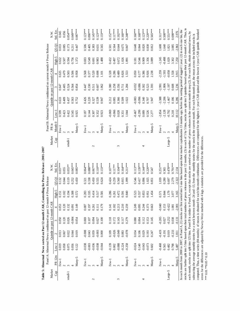
3.1 Controlling for Press Release

The tests here include press releases as controls. Press releases originate from firms and their frequency

represents a willingness to share firm-specific information.

In Table 5, abnormal news coverage is conditioned on the number of press releases from a firm in the

current month and in the past 12 months. In Panel A, stocks are first split into five bins based on their

market capitalization at the end of month -13. Then each bin is further split into five bins based on the

total number of press releases in the past 12 months. Finally, each of the 25 bins are sorted into five

quintiles based on their past 12-month CAR. Panel B is similar to Panel A, except the conditioning is set

on the press release in the current month. The date range is from 2000 to 2007. Dow Jones News Service

only includes press releases after 1999. I start the analysis on 2001, and this leaves a time-series length of

84 months.

Panel A and Panel B both shows, even when controlling for press releases in the past 12 month and in the

current month, the effects of the past 12-month CAR on current abnormal coverage are not changed. The

differences between the low past return quintile and the high past return quintile remain highly

statistically significant. The standard errors are estimated with Newey-West methods with four lags. This

suggests that the long-run media coverage bias is robust.

To investigate the effect of press releases alone, Table 6 checks the effects of past 12-month press

releases and current press releases on current abnormal news. In Table 6, stocks first are sorted into five

cap bins based on market capitalization in month -13. Each cap bin is split into five past 12-month CAR

bins. After conditioning on the market cap and the past 12-month CAR, the effects of past 12-month press

releases and current press releases are examined in Panel A and Panel B specifically. Panel A indicates

that past press releases have little impact on current abnormal news, while Panel B indicates that the

effect of current month press releases is strong. This indicates that press releases have only a

contemporaneous correlation with current abnormal coverage. This does not necessarily imply that press

releases generate current news coverage. Following any events from a firm, its press release and it

experiences increased mediacurrent news coverage, but are likely to increase temporarily at the two are

not necessarily in a causal relationship. Any effect of press releases on media coverage is likely to be

contemporaneous, that is, past press releases are unlikely to influence future media coverage. This greatly

reduces the chance that press releases are the major driver behind the long-run coverage bias. Solomon

and Soltes (2011) find that the largest determinants of media coverage likely are outside managerial

control. Our results support this argument.

Low

-12

34

Hig

h-5

Q5-

Q1

Low

-12

34

Hig

h-5

Q5-

Q1

Few

-10.

019

0.01

30.

050

0.05

30.

151

0.13

20.

037*

**Fe

w-1

0.59

90.

633

0.64

70.

635

0.63

20.

033

0.04

52

0.05

80.

067

0.12

00.

120

0.10

20.

044

0.05

52

0.42

30.

409

0.40

50.

479

0.50

70.

085

0.05

63

0.07

50.

022

0.02

60.

132

0.19

40.

119

0.05

5**

30.

422

0.43

70.

524

0.50

30.

594

0.17

30.

054*

**4

0.05

60.

044

-0.0

040.

091

0.30

80.

252

0.04

5***

40.

545

0.56

30.

564

0.50

60.

756

0.21

10.

049*

**M

any-

50.

122

0.01

90.

054

0.14

90.

572

0.45

00.

085*

**M

any-

50.

925

0.75

20.

854

0.95

81.

372

0.44

70.

087*

**

Few

-1-0

.038

-0.0

080.

069

0.08

70.

283

0.32

10.

064*

**Fe

w-1

0.18

70.

426

0.44

70.

568

0.69

30.

506

0.12

3***

2-0

.003

0.04

30.

107

0.19

70.

335

0.33

80.

088*

**2

0.14

40.

220

0.33

00.

377

0.54

90.

405

0.09

0***

3-0

.036

0.05

90.

094

0.26

10.

414

0.45

00.

067*

**3

0.30

70.

327

0.51

10.

520

0.69

10.

383

0.14

5***

4-0

.038

-0.0

030.

027

0.11

10.

517

0.55

50.

110*

**4

0.35

20.

539

0.60

70.

698

0.98

30.

631

0.12

3***

Man

y-5

-0.0

440.

000

0.10

00.

179

0.58

10.

624

0.13

3***

Man

y-5

0.92

30.

947

1.06

21.

101

1.48

80.

565

0.13

3***

Few

-1-0

.139

0.10

90.

118

0.14

10.

286

0.42

40.

107*

**Fe

w-1

-0.0

690.

212

0.38

00.

328

0.43

20.

501

0.15

2***

20.

002

-0.0

260.

172

0.18

20.

261

0.25

90.

117*

*2

-0.0

660.

085

0.25

80.

286

0.49

70.

564

0.11

7***

3-0

.088

-0.0

490.

143

0.21

30.

472

0.56

00.

104*

**3

0.02

80.

366

0.35

60.

489

0.67

20.

644

0.19

2***

4-0

.224

0.08

30.

117

0.21

00.

591

0.81

50.

164*

**4

0.35

10.

509

0.71

10.

826

1.02

60.

675

0.16

0***

Man

y-5

-0.2

58-0

.078

0.27

90.

259

0.84

01.

099

0.21

1***

Man

y-5

1.04

41.

022

1.28

41.

553

1.89

10.

847

0.24

8***

Few

-1-0

.024

0.03

40.

080

0.24

90.

523

0.54

60.

113*

**Fe

w-1

-0.4

67-0

.083

-0.0

320.

050

0.18

10.

648

0.16

0***

20.

140

0.10

60.

004

0.09

50.

557

0.41

70.

139*

**2

-0.2

99-0

.096

-0.0

860.

177

0.54

60.

844

0.16

8***

3-0

.043

0.02

90.

112

0.24

40.

853

0.89

60.

144*

**3

0.08

90.

340

0.30

20.

386

0.90

90.

820

0.12

3***

4-0

.073

0.19

30.

153

0.37

30.

951

1.02

50.

220*

**4

0.52

60.

707

0.52

30.

926

1.35

60.

830

0.22

0***

Man

y-5

0.60

20.

247

0.14

50.

663

1.45

40.

851

0.54

7M

any-

52.

277

1.94

71.

593

2.23

83.

089

0.81

20.

565*

**

Few

-1-0

.468

-0.4

19-0

.205

-0.0

400.

571

1.03

90.

251*

**Fe

w-1

-2.8

54-3

.388

-2.9

91-2

.259

-1.2

451.

608

0.31

1***

20.

565

-0.1

910.

027

0.15

30.

844

0.28

00.

365

2-2

.128

-2.2

06-1

.806

-1.5

93-0

.488

1.64

00.

508*

**3

0.48

20.

019

-0.2

52-0

.422

1.17

90.

697

0.47

8***

3-0

.792

-1.4

67-1

.197

-0.0

581.

029

1.82

10.

551*

**4

0.79

8-0

.233

0.03

81.

081

3.07

72.

279

0.79

1***

40.

218

0.18

60.

608

1.55

83.

302

3.08

50.

698*

**M

any-

55.

487

1.81

1-0

.131

-2.0

013.

165

-2.3

222.

134

Man

y-5

10.1

126.

286

5.23

63.

915

7.25

0-2

.861

2.07

6

Tab

le 5

: A

bnor

mal

New

s so

rted

on

Pas

t 12

-mon

th C

AR

, Con

trol

ling

for

Pre

ss R

elea

se:

2001

-200

7

Pan

el A

: Abn

orm

al N

ews

cond

ition

ed o

n pa

st 1

2-m

onth

# P

ress

Rel

ease

Pan

el B

: Abn

orm

al N

ews

cond

ition

ed o

n cu

rren

t mon

th #

Pre

ss R

elea

seN

.W.

Std.

Err

.

smal

l-1

2

33

Mar

ket

Cap

PR

12m

Qui

ntile

on

past

12-

mon

th C

AR

N.W

.St

d. E

rr.

Mar

ket

Cap

PR

inM

onth

0Q

uint

ile o

n pa

st 1

2-m

onth

CA

R

4

Lar

ge-5

Lar

ge-5

In e

ach

mon

th f

rom

200

0 to

200

7, in

Pan

el A

, (1)

sto

cks

are

first

sor

ted

into

5 s

ize

bins

bas

ed u

pon

thei

r m

arke

t cap

italiz

atio

n 13

mon

ths

ago,

bef

ore

the

sort

ing

perio

d of

lagg

ed 1

yea

r; (

2) in

eac

h si

ze b

in, t

he

stoc

ks a

re f

urth

er s

plit

into

5 b

ins

base

d up

on th

eir

tota

l num

bers

of

pres

s re

leas

es in

the

past

12

mon

ths;

(3)

in e

ach

of 5

by

5 bi

ns, s

tock

s ar

e sp

lit in

to 5

qui

ntile

s ba

sed

upon

thei

r pa

st 1

2-m

onth

CA

R. T

hus,

in

each

mon

th, s

tock

s ar

e sp

lit in

to 1

25 b

ins.

Pan

el B

is s

imila

r to

Pan

el A

, exc

ept t

hat s

tock

s ar

e so

rted

on

the

num

ber

of p

ress

rel

ease

s in

the

curr

ent m

onth

in s

tep

(2).

For

eac

h bi

n, o

btai

n ab

norm

al n

ews,

by

subt

ract

ing

the

aver

age

mon

thly

sto

ries

for

a st

ock

betw

een

mon

th -

24 a

nd -

13, f

rom

the

mon

thly

sto

ries

for

the

stoc

k in

the

curr

ent m

onth

. For

eac

h bi

n-m

onth

pai

r, th

e m

ean

acro

ss th

e in

clud

ed s

tock

s is

co

mpu

ted.

Thu

s, a

tim

e se

ries

(84

mon

ths)

of

mea

ns is

obt

aine

d fo

r ea

ch b

in-m

onth

com

bina

tion.

Diff

eren

ces

are

com

pute

d fo

r th

e hi

ghes

t 1-

year

CA

R q

uint

al a

nd th

e lo

wes

t 1-y

ear

CA

R q

uint

ile. S

tand

ard

erro

rs f

or th

e di

ffer

ence

s ar

e ad

just

ed b

y N

ewey

-Wes

t met

hod

with

4 la

gs. t

-sta

tistic

s ar

e pr

ovid

ed f

or th

e di

ffer

ence

s.

***

0.01

**0

.05

* 0.

10

smal

l-1

2 4

Few

-12

34

Man

y-5

Q5-

Q1

Few

-12

34

Man

y-5

Q5-

Q1

Low

-10.043

0.073

0.040

0.092

0.075

0.03

30.

102

Low

-10.623

0.391

0.498

0.560

0.929

0.30

60.

67*

20.014

0.092

0.017

0.023

‐0.010

-0.0

230.

061

20.622

0.337

0.457

0.504

0.749

0.12

80.

148

30.047

0.138

0.072

0.019

0.051

0.00

40.

059

30.630

0.523

0.408

0.640

0.743

0.11

30.

115

40.055

0.102

0.096

0.076

0.117

0.06

10.

074

40.692

0.448

0.442

0.565

0.893

0.20

00.

140

Hig

h-5

0.176

0.117

0.268

0.292

0.529

0.35

30.

113*

**H

igh-

50.661

0.551

0.623

0.674

1.362

0.70

10.

214*

**

Low

-1‐0.044

0.017

‐0.058

‐0.078

‐0.040

0.00

40.

148

Low

-10.191

0.083

0.320

0.436

1.008

0.81

70.

214*

**2

0.047

0.025

0.017

0.027

‐0.020

-0.0

680.

119

20.468

0.217

0.356

0.529

0.839

0.37

00.

123*

*3

0.017

0.069

0.106

0.047

0.043

0.02

60.

104

30.550

0.216

0.366

0.669

0.832

0.28

13.

32**

*4

0.157

0.271

0.176

0.209

0.274

0.11

70.

118

40.614

0.420

0.549

0.657

1.191

0.57

80.

220*

**H

igh-

50.284

0.414

0.391

0.507

0.453

0.16

80.

143

Hig

h-5

0.599

0.524

0.764

0.974

1.446

0.84

70.

216*

**

Low

-1‐0.096

‐0.067

‐0.210

‐0.223

‐0.195

-0.1

000.

214

Low

-10.044

‐0.186

0.006

0.400

1.008

0.96

40.

310*

**2

0.064

‐0.026

‐0.075

0.003

0.120

0.05

70.

178

20.252

0.045

0.244

0.572

1.087

0.83

40.

270*

**3

0.082

0.185

0.101

0.184

0.143

0.06

20.

141

30.349

0.282

0.470

0.605

1.209

0.85

90.

239*

**4

0.200

0.141

0.199

0.209

0.362

0.16

20.

177

40.409

0.277

0.431

0.724

1.394

0.98

40.

278*

**H

igh-

50.281

0.396

0.485

0.579

0.793

0.51

20.

219*

*H

igh-

50.514

0.437

0.769

1.068

1.912

1.39

80.

331*

**

Low

-10.077

0.049

‐0.018

‐0.122

0.752

0.67

50.

736

Low

-1‐0.456

‐0.238

0.110

0.469

2.611

3.06

70.

780*

**2

0.001

0.095

‐0.014

0.147

0.066

0.06

50.

323

2‐0.072

‐0.196

0.326

0.479

1.647

1.72

00.

376*

**3

0.025

‐0.044

0.051

0.214

0.318

0.29

30.

331

3‐0.074

‐0.066

0.261

0.606

1.656

1.73

00.

346*

**4

0.254

0.211

0.210

0.254

0.716

0.46

20.

284

40.135

0.134

0.462

0.748

2.054

1.92

00.

353*

**H

igh-

50.595

0.641

0.940

0.836

1.407

0.81

20.

450

Hig

h-5

0.295

0.604

0.948

1.280

3.098

2.80

30.

596*

**

Low

-1‐0.235

0.525

0.147

0.107

6.180

6.41

55.

172

Low

-1‐2.727

‐1.960

‐0.644

1.272

10.764

13.4

904.

238*

**2

‐0.367

‐0.216

0.050

‐0.626

0.980

1.34

76.

097

2‐3.421

‐2.334

‐1.444

0.013

6.957

10.3

774.

170*

*3

‐0.352

‐0.265

0.013

0.201

‐1.224

-0.8

724.

480

3‐2.889

‐2.120

‐1.006

0.292

3.950

6.83

93.

459*

4‐0.097

0.080

0.046

0.664

0.226

0.32

43.

682

4‐2.460

‐1.502

‐0.171

0.803

4.131

6.59

12.

838*

*H

igh-

50.735

1.122

0.981

2.977

3.010

2.27

42.

907

Hig

h-5

‐1.120

‐0.490

1.058

2.669

7.320

8.44

02.

452*

**

33

Tab

le 6

: C

hang

e in

Num

ber

of S

tori

es r

epor

ted

sort

ed o

n P

ress

Rel

ease

s in

par

t 12

Mon

ths

and

in C

urre

nt M

onth

: 20

01-2

007

Pan

el A

: Abn

orm

al N

ews

cond

ition

ed o

n pa

st 1

2-m

onth

# P

ress

Rel

ease

Pan

el B

: Abn

orm

al N

ews

cond

ition

ed o

n cu

rren

t mon

th #

Pre

ss R

elea

seM

arke

t C

ap12

-mon

th

CA

RQ

uint

ile o

n pa

st 1

2-M

onth

#P

RN

.W.

Std.

Err

.M

arke

t C

ap12

-mon

th

CA

RQ

uint

ile o

n cu

rren

t mon

th #

PR

N.W

.St

d. E

rr.

smal

l-1sm

all-1

22

44

Lar

ge-5

Lar

ge-5

In P

anel

A, i

n ea

ch m

onth

fro

m 2

001

to 2

007,

(1)

sto

cks

are

sort

ed in

to 5

siz

e bi

ns b

ased

upo

n th

eir

mar

ket c

apita

lizat

ion

13 m

onth

s ag

o, b

efor

e th

e so

rtin

g pe

riod

of la

gged

1 y

ear;

(2)

in e

ach

size

bin

, sto

cks

are

split

into

5 q

uint

iles

base

d up

on th

eir

1-ye

ar la

gged

CA

R; (

3) in

eac

h of

5 b

y 5

bins

, the

sto

cks

are

furt

her

split

into

5 b

ins

base

d up

on th

eir

tota

l num

bers

of

pres

s re

leas

es in

the

past

12

mon

ths.

In

Pan

el

B, t

he s

ortin

g st

eps

are

the

the

sam

e in

(1)

and

(2)

. In

step

(3)

, the

sto

cks

are

furt

her

split

into

5 b

ins

base

d up

on th

eir

num

bers

of

pres

s re

leas

es in

the

curr

ent m

onth

. In

each

mon

th, s

tock

s ar

e sp

lit in

to 1

25

bins

in b

oth

pane

ls. F

or e

ach

bin,

obt

ain

the

abno

rmal

, by

subt

ract

ing

the

aver

age

mon

thly

sto

ries

for

a st

ock

betw

een

mon

th -

24 a

nd -

13, f

rom

the

mon

thly

sto

ries

for

the

stoc

k in

the

curr

ent m

onth

. For

eac

h bi

n-m

onth

pai

r, th

e m

ean

acro

ss th

e in

clud

ed s

tock

s is

com

pute

d. T

hus,

a ti

me

serie

s (8

4 m

onth

s) o

f m

eans

is o

btai

ned

for

each

bin

-mon

th c

ombi

natio

n. D

iffer

ence

s ar

e co

mpu

ted

for

the

high

est p

ress

re

leas

e qu

intil

e an

d th

e lo

wes

t pre

ss r

elea

se q

uint

ile. t

-sta

tistic

s us

ing

New

ey-W

est a

djus

ted

stan

dard

err

ors

(4 la

gs)

are

prov

ided

for

the

diff

eren

ces.

***

0.01

**0

.05

* 0.

10

3.2 Earnings News

Solomon (2011) argues that earnings information is “hard information,” which is less likely to be

influenced by firms’ IR activities. If the long term bias were introduced by a firm’s IR activities, the bias

should diminish or disappear in earnings news coverage.

DJNS provides two tags on news. One tag is “press release,” which indicates that a story is issued by a

firm itself. The other tag is “earnings,” which indicates that a story falls into the category of earning news.

Using these two tags, I can locate the firms’ press releases on earnings. A subset of 89,535 earnings press

releases is identified. The available date range is from 2000 to 2007. The earnings releases generally are

distributed in January, April, July, and October. For most firms, the releases are issued usually once a

quarter or less frequent.

Following each earnings press release, from day 0 to day 6 I count the stories that have the earnings tag

but are not press releases. The observation window is set to the week from the day of an earnings

announcement to six days from the announcement date. The media’s coverage on earnings in this time

frame is likely to be reports on the most recent earnings announcement. Follow-up earnings likely result

in media “mentions” of the recent earnings event.

In Table 7, the stocks are first conditioned on market cap in month -13 prior to the 12-month sorting

period. In Panel A, stocks in each size bin are then conditioned on a seven-day CAR following the

announcement and, finally, each of 25 bins is split into another five bins based on the past 12-month

CAR. An 84-month time series of differences between the high past return quintile and the low past

return quintile is generated for the 25 bins. I use bootstrapping methods to obtain p-values for whether the

differences are significantly different from zero. Panel A allows us to examine if the long-run bias exists

within the earnings follow-up coverage. That is, do the media give more attention to earnings releases

from stocks that performed well in the past? The answer is yes. In 23 out of 25 conditioning bins, high

past 12-month CAR quintiles receive more earnings news coverage than low past 12-month CAR

quintiles. The bootstrapping statistics are significant for most situations. While the significance drops

slightly relative to Table 2, this is not surprising because stock-day pairs in quintile 5 may not be in the

same time as quintile 1. As a result, the time-series upward trend in news coverage increases the standard

deviations of the differences. Overall, Table 7 Panel A supports Table 2 at a different level: the

documented long-run bias is unlikely introduced by firms themselves.

Panel B examines the effect of post-earnings drift on earnings news coverage, conditioning on market cap

and past 12-month CAR. The top post 1-week CAR quintiles likely are earnings announcements above

expectation and the bottom quintiles likely are announcements below expectation. Panel B shows how the

media covers events in the short run. As can be seen, the top quintiles and the bottom quintiles receive

about the same “mentions” on their earnings releases. That is, bad earnings announcements and good

earnings announcements receive about the same number of media follow-up reports. However, both

extreme quintiles receive more “mentions” than the middle quintiles. Thus, media coverage is biased

toward “surprises” in the short run. This is very consistent with Solomon and Soltes (2011). In their

study, the press (paper) coverage is more intensive on extreme daily contemporaneous returns7.

                                                            7 Solomon and Soltes (2011) find that paper press also tends to emphasize bad news. Our results only have slight support for this and do not hold much statistical significance.

Low

-12

34

Hig

h-5

Q5-

Q1

Low

-12

34

Hig

h-5

Q5-

Q1

Q1-

Q3

Q5-

Q3

Low

-10.

854

0.81

30.

831

0.79

10.

943

0.08

9**

Low

-10.

856

0.75

60.

618

0.71

80.

836

-0.0

200.

238*

**0.

218*

**2

0.72

90.

729

0.62

40.

699

0.71

8-0

.01

20.

813

0.67

20.

583

0.65

00.

787

-0.0

260.

230*

**0.

204*

**3

0.59

50.

600

0.59

00.

613

0.70

40.

109*

**3

0.79

90.

626

0.59

40.

660

0.76

7-0

.032

0.20

6***

0.17

4***

40.

709

0.65

80.

653

0.67

20.

660

-0.0

494

0.80

10.

693

0.62

60.

676

0.80

70.

006

0.17

4***

0.18

1***

Hig

h-5

0.83

00.

807

0.79

90.

845

0.86

40.

034

Hig

h-5

0.94

30.

744

0.71

20.

696

0.89

7-0

.046

0.23

1***

0.18

5***

Low

-10.

951

1.01

81.

027

1.01

01.

066

0.11

5***

Low

-10.

990

0.83

00.

760

0.77

40.

920

-0.0

69*

0.23

0***

0.16

1***

20.

796

0.78

40.

805

0.82

40.

820

0.02

42

1.00

30.

765

0.71

90.

709

0.94

0-0

.063

*0.

284*

**0.

220*

**3

0.74

90.

718

0.70

80.

790

0.82

20.

073*

30.

981

0.81

10.

674

0.75

20.

954

-0.0

270.

307*

**0.

281*

**4

0.75

30.

749

0.75

50.

808

0.88

10.

127*

**4

0.98

80.

817

0.80

10.

804

0.97

3-0

.015

0.18

8***

0.17

3***

Hig

h-5

0.90

40.

947

0.99

00.

981

1.04

10.

137*

**H

igh-

51.

081

0.86

60.

829

0.89

11.

066

-0.0

150.

253*

**0.

238*

**

Low

-11.

078

1.17

81.

226

1.25

71.

406

0.32

8***

Low

-11.

126

0.96

50.

902

0.97

51.

139

0.01

30.

223*

**0.

236*

**2

0.95

70.

942

0.98

81.

038

1.07

80.

121*

*2

1.19

20.

959

0.85

90.

907

1.21

40.

022

0.33

3***

0.35

5***

30.

895

0.85

50.

870

0.92

01.

006

0.11

1**

31.

201

0.96

90.

877

0.95

61.

210

0.00

90.

324*

**0.

332*

**4

0.94

50.

926

1.01

30.

990

1.06

20.

117*

*4

1.24

40.

996

0.91

41.

019

1.23

2-0

.012

0.33

0***

0.31

8***

Hig

h-5

1.13

31.

217

1.19

81.

263

1.29

70.

164*

**H

igh-

51.

413

1.09

01.

010

1.06

81.

304

-0.1

08*

0.40

2***

0.29

4***

Low

-11.

434

1.54

81.

560

1.62

91.

773

0.33

9***

Low

-11.

451

1.30

51.

126

1.31

01.

437

-0.0

140.

325*

**0.

311*

**2

1.25

41.

240

1.25

31.

232

1.45

30.

199*

**2

1.57

81.

167

1.19

61.

286

1.54

1-0

.036

0.38

1***

0.34

5***

31.

097

1.15

21.

123

1.25

41.

245

0.14

7**

31.

555

1.23

31.

131

1.24

21.

490

-0.0

660.

424*

**0.

358*

**4

1.31

31.

263

1.32

91.

273

1.45

90.

146*

*4

1.60

91.

219

1.24

21.

275

1.50

9-0

.100

0.36

7***

0.26

7***

Hig

h-5

1.39

11.

560

1.47

91.

544

1.71

80.

327*

**H

igh-

51.

770

1.44

01.

270

1.47

11.

727

-0.0

420.

499*

**0.

457*

**

Low

-12.

281

2.87

12.

996

3.05

12.

666

0.38

5***

Low

-12.

320

2.49

02.

572

2.64

72.

564

0.24

4*-0

.252

*-0

.008

***

22.

425

2.80

92.

831

2.79

72.

528

0.10

32

2.89

12.

741

2.39

22.

800

2.74

2-0

.149

0.49

9***

0.35

0***

32.

508

2.43

62.

609

2.44

62.

374

-0.1

353

2.96

62.

858

2.55

72.

766

3.00

40.

038

0.40

9***

0.44

8***

42.

707

2.78

32.

840

2.86

12.

770

0.06

34

2.99

22.

838

2.48

32.

850

3.08

40.

092

0.50

8***

0.60

1***

Hig

h-5

2.50

62.

851

2.90

83.

047

2.95

00.

444*

**H

igh-

52.

633

2.60

22.

346

2.75

52.

962

0.32

9**

0.28

8**

0.61

6***

From

200

0 to

200

7, a

sub

set o

f st

ock-

day

pairs

with

firm

rel

easi

ng e

arni

ng n

ews

are

obta

ined

. Dow

Jon

e N

ews

Serv

ices

pro

vide

s ta

gs o

n fir

ms'

pre

ss r

elea

se a

nd e

arni

ngs

new

s. I

n P

anel

A, a

mon

g th

e se

lcte

d st

ock-

days

pai

rs, (

1) s

tock

s ar

e so

rted

into

5 s

ize

bins

bas

ed u

pon

thei

r m

arke

t cap

italiz

atio

n 13

mon

ths

ago;

(2)

in e

ach

size

bin

, the

sto

cks

are

furt

her

split

into

5 b

ins

base

d up

on 1

wee

k C

AR

fro

m

day

0 to

day

6; (

3) in

eac

h of

5 b

y 5

bins

, sto

cks

are

split

into

5 q

uint

iles

base

d up

on th

eir

past

12-

mon

th C

AR

. Thu

s, a

ll th

e se

lect

ed s

tock

-day

pai

rs a

re s

plit

into

125

bin

s. T

he s

torie

s w

ith e

arni

ngs

tag

are

repo

rted

and

thes

e st

orie

s ar

e lik

ely

to r

epea

t the

sto

ck's

rec

ent e

arni

ng r

elea

se. I

n P

anel

B, t

he s

ortin

g st

eps

(2)

and

(3)

are

swap

ed a

nd th

is r

evea

ls th

e co

nditi

onal

impa

ct o

f po

st a

nnou

cem

ent C

AR

. In

Pan

el A

, Diff

eren

ces

are

com

pute

d fo

r hi

gh-5

12-

mon

th C

AR

qui

ntile

and

low

-1 1

2-m

onth

CA

R q

uint

ile. I

n P

anel

B, t

he m

ain

sort

ing

varia

ble

is p

ost a

nnou

cem

ent d

rift.

The

diff

eren

ce b

etw

een

Q5

and

Q1,

be

twee

n Q

1 an

d Q

3, a

nd b

etw

een

Q5

and

Q3

are

com

pute

d. T

he ti

me

serie

s sp

an 8

4 m

onth

s. B

oots

trap

ping

test

sta

tistic

s ar

e us

ed to

che

ck th

e si

gnifi

canc

e of

the

dife

renc

es.

***

0.01

**0

.05

* 0.

10

Pan

el A

: Med

ia F

ollo

w-u

ps c

ondi

tione

d on

pas

t 12-

mon

th C

AR

33

44

Lar

ge-5

Lar

ge-5

Qui

ntile

on

Pos

t 1-w

eek

CA

R

smal

l-1sm

all-1

22

Mar

ket

Cap

Pos

t 1-

wee

k C

AR

Qui

ntile

on

past

12-

mon

th C

AR

Mar

ket

Cap

past

12-

mon

th

CA

R

Tab

le 7

: N

umbe

r of

Ear

ning

s N

ews

follo

win

g F

irm

's E

arni

ngs

Pre

ss R

elea

se, 2

001-

2007

Pan

el B

: Med

ia F

ollo

w-u

ps c

ondi

tione

d on

pos

t 1-w

eek

CA

R

4. Discussion

I find a long-run media coverage bias toward high returns and a short-run bias toward extreme returns.

The long-run bias occurs only for stale news, probably because the media revisits only past winners. I

show that the biases are robust against the influence of supply preferences, indicating that the main driver

comes from the demand side.

4.1 Reconciliation with other studies

Our results suggest that the media coverage can be affected by both supply bias and demand bias, but the

supply factors have only a short-lived impact. I show that contemporaneous press releases are correlated

with abnormal news coverage. This is consistent with Solomon (2011), Gurun (2010), and Gurun and

Bulter (2010). Yet past press releases have little impact on contemporaneous abnormal news coverage.

The long-run coverage bias toward high historic returns likely is driven by demand factors.

Our study examines returns in much longer time horizons. Other studies have looked only at returns for

very short windows, most at daily frequencies. I extend the return sorting window and identify the long-

run coverage bias.

Our short-run bias findings agree with other studies. I show that in event weeks, the media pays higher

attention to extreme returns. This is consistent with the sensationalism argument of Solomon and Soltes

(2011). Following event weeks, the media revisits outperforming stocks at higher than average levels and

revisit underperforming stocks at lower than average levels. This suggests that media attention on

underperformance is short-lived. It can be reasonably assumed that extreme loss might shock investors

initially, but the effect of sensationalism drops fast with repetition.

These results open the question of why the media chooses to revisit outperforming stocks.

4.2 Possible explanations

Why is the media more inclined to report on past winners? I have shown above that this phenomenon is

not driven by supply bias—that is by firm press releases, though it is affected by contemporaneous

supply. I conjecture that it is, instead, driven mostly by investors' preferences for information relevant to

their investment decisions.

Below I extend a few conjectures, which needs further verification and are currently beyond the domain

of this study.

(1) The scope of interested investors. When the media tells subscribers that a certain stock is

outperforming, it is likely to arouse the interest of all investors; when the media reports on an

underperforming stock, it may only interest those who have stakes in the stock given the short-

selling constraints. Watchers of Jim Cramer’s show are hoping to get tips more on stocks to buy,

less on stocks to sell.

(2) Representative Bias. Investors may look into the characteristics of the outperforming stocks with

the hope of understanding why they outperformed and how to identify a new opportunity. The

representative heuristic might lead them to believe these stocks will continue to outperform. For

the poor performing stocks, they surely have less interest.

(3) Chasing past returns. Grinblatt et al (1995) reveal that mutual funds chase past winners.

Newswire subscribers are mostly investment professionals. If they seek to chase past returns, they

prefer their media to cover more stories on the winning stocks.

(4) Brag and look smart. Suppose media covers the prospects of two stocks intensively at a given

time. A year later, one of the stocks skyrockets and the other plummets. If readers of the first

story purchased the first stock mentioned in the story and readers of the second story purchased

the other stock, the media is more likely to repeat the previous story (or even cite their foresight).

Repeating stories on the first stock would emphasize that the media provided investors with a

valuable piece of investment information. The media may choose to avoid mentioning the

underperforming stock again to avoid blame for investors’ losses.

(5) Regret and Shame. Barber, Odean and Strahilevitz (2011) find that retail investors’ purchasing

behavior exhibit patterns of emotions. They repurchase stocks whose previous purchase resulted

in positive emotions and avoid stocks whose previous purchase resulted in negative emotions. IT

seems reasonable that investors would spontaneously pay attention to past winners simply

because they just missed the opportunities. With regard to losers, those without stakes in the

stocks would not experience regret in hearing about them; but those with stakes would find the

attention yo the losers painful. 

5. Conclusions

This study demonstrates that the media has a long-run coverage bias toward high returns, and a short-run

bias toward extreme returns. The long-run bias is robust after controlling for market capitalization,

contemporaneous return, P/E ratio, analyst coverage, press releases (both contemporaneous and historic),

and industry fixed effect.

I show that the long-run bias mostly is on repetitive news, not fresh news, and the short run bias occurs

for contemporaneous news events. Our conjecture is that the short-run bias is driven by a sensationalism

bias. Investors naturally tune in to fresh, shocking news. However, once the shock period is over,

investors would lose interest in the losers. As shown, post-shock coverage on both types of extreme

returns drops. This is consistent with the sensationalism bias argued by Solomon and Soltes (2011). After

the shock stage, investors have to reassess the information they would like to access. Media coverage on

positive returns sustains at high levels and drops fastest on negative returns, indicating that investors

probably are more interested in winners, possibly because the stocks they are thinking of buying or have

recently bought more often than not have strong past performance.

The long-run bias I identify is important to the literature of attention-driven investment behaviors. When

our results are compared with those of Fang and Peress (2010), a much bigger picture of the coverage-

return relationship emerges. Fang and Peress (2010) find that stocks covered intensively tend to have low

future returns, and I show that high coverage stocks tend to have high past returns. This calls into

question their explanations. Future research could contribute to an understanding long-term return

reversal in relation to media coverage.

Reference

Barber, Brad M. and Terrence Odean, (2008), “All that Glitters: The Effect of Attention and News on the Buying Behavior of Individual and Institutional Investors”, Review of Financial Studies, 21 (2), 785-818 Bushee, Brian J. and Gregory S. Miller, (2007), “Investor Relations, Firm Visibility, and Investor Following”, Working Paper Chan, Wesley S. (2003), “Stock price reaction to news and no-news: drift and reversal after headlines”, Journal of Financial Economics, 70 (2), 223-260 Da, Zhi, Joseph Engelberg and Pengjie Gao, (2011), In search of attention, Journal of Finance, Forthcoming

DellaVigna, Stefano, and Joshua Pollet, (2009), “Investor Inattention and Friday Earnings Announcements”, Journal of Finance, 64 (2) 709-749 Engelberg, Joseph and Christopher A. Parsons (2010), “The Causal Impact of Media in Financial Markets”, Journal of Finance, Forthcoming Fang, Lily H., and Joel Peress, (2009), “Media Coverage and the Cross-Section of Stock Returns”, Journal of Finance, 64 (5), 2023-2052 Grinblatt, Mark, Sheridan Titman and Russ Wermers, (1995), Momentum Strategies, Portfolio Performance, and Herding: A Study of Mutual Fund Behavior, American Economic Review, 85(5), 1088-1105 Gurun, Umit G. and Alexander W. Butler, (2010), “Don’t Believe the Hype: Local Media Slant, Local Advertising, and Firm Value”, Journal of Finance, Forthcoming Hamilton, J. (2004), All the News That’s Fit to Sell: How the Market Transforms Information to News.Princeton University Press, New Jersey, USA. Odean, Terrance, Brad Barber and Michal Strahilevitz, (2011), “Once Burned, Twice Shy: How Naïve Learning, Counterfactuals, and Regret Affect the Repurchase of Stocks Previously Sold”, Jounrnal of Marketing Research, Forthcoming

Solomon, David H. (2010), “Selective Publicity and Stock Prices”, Journal of Finance, Forthcoming Solomon, David H. and Eugene F. Soltes (2011), “The Determinants of Coverage in the Business Press”, Working Paper Tetlock, Paul C. (2010a), “Does Public Financial News Resolve Asymmetric Information”, Review of Financial Studies, 23 (9), 3520-3557

Tetlock, Paul C. (2010b), “All the News That’s Fit to Reprint: Do Investors React to Stale Information?”, Review of Financial Studies, Forthcoming