LUND UNIVERSITY

PO Box 117221 00 Lund+46 46-222 00 00

Stochastic Theory of Continuous-Time State-Space Identification

Johansson, Rolf; Verhaegen, Michel; Chou, C. T.

Published in:IEEE Transactions on Signal Processing

DOI:10.1109/78.738238

1999

Document Version:Publisher's PDF, also known as Version of record

Link to publication

Citation for published version (APA):Johansson, R., Verhaegen, M., & Chou, C. T. (1999). Stochastic Theory of Continuous-Time State-SpaceIdentification. IEEE Transactions on Signal Processing, 47(1), 41-51. https://doi.org/10.1109/78.738238

General rightsCopyright and moral rights for the publications made accessible in the public portal are retained by the authorsand/or other copyright owners and it is a condition of accessing publications that users recognise and abide by thelegal requirements associated with these rights.

• Users may download and print one copy of any publication from the public portal for the purpose of private studyor research. • You may not further distribute the material or use it for any profit-making activity or commercial gain • You may freely distribute the URL identifying the publication in the public portalTake down policyIf you believe that this document breaches copyright please contact us providing details, and we will removeaccess to the work immediately and investigate your claim.

IEEE TRANSACTIONS ON SIGNAL PROCESSING, VOL. 47, NO. 1, JANUARY 1999 41

Stochastic Theory of Continuous-TimeState-Space Identification

Rolf Johansson, Michel Verhaegen, and Chun Tung Chou

Abstract—This paper presents theory, algorithms, and vali-dation results for system identification of continuous-time state-space models from finite input–output sequences. The algorithmsdeveloped are methods of subspace model identification andstochastic realization adapted to the continuous-time context.The resulting model can be decomposed into an input–outputmodel and a stochastic innovations model. Using the Riccatiequation, we have designed a procedure to provide a reduced-order stochastic model that is minimal with respect to systemorder as well as the number of stochastic inputs, thereby avoidingseveral problems appearing in standard application of stochasticrealization to the model validation problem.

Index Terms—Continuous time, state-space system, systemidentification.

I. INTRODUCTION

T HE LAST FEW years have witnessed a strong interest insystem identification using realization-based algorithms.

The use of Markov parameters as suggested by Ho andKalman [13], Akaike [1], and Kung [20] of a system can beeffectively applied to the problem of state-space identification;see Verhaegenet al. [30], [31], van Overschee and de Moor[28], Juang and Pappa [19], Moonenet al. [26], and Bayard[3], [4], [23], [24]. Suitable background for the discrete-timetheory supporting stochastic subspace model identification isto be found in [1], [10], and [28]. As for model structures andrealization theory, see the important contributions in [8] and[22]. As these subspace-mode identification algorithms dealwith the case of fitting a discrete-time model, it remains as anopen problem how to extend these methods for continuous-time systems. A great deal of modeling in natural sciences andtechnology is made by means of continuous-time models andsuch models require suitable methods of system identification[14]. To this end, a theoretical framework of continuous-timeidentification and statistical model validation is needed. In

Manuscript received January 15, 1997; revised May 11, 1998. This workwas supported by the H¨orjel Foundation and the National Board for Industrialand Technical Development (NUTEK). The associate editor coordinating thereview of this paper and approving it for publication was Dr. Yingbo Hua.

R. Johansson is with the Department of Automatic Control, LundInstitute of Technology, Lund University, Lund, Sweden (e-mail:Rolf.Johansson@control.lth.se).

M. Verhaegen and C. T. Chou are with the Department of ElectricalEngineering, System and Control Engineering Group, Delft, The Netherlands(e-mail: M.Verhaegen@et.tudelft.nl).

Publisher Item Identifier S 1053-587X(99)00137-3.

particular, as experimental data are usually provided as timeseries, it is relevant to provide continuous-time theory andalgorithms that permit application to discrete-time data.

This paper treats the problem of continuous-time systemidentification based on discrete-time data and provides aframework with algorithms presented in preliminary forms in[11], [16], and [17]. The approach adopted is that of subspace-model identification [18], [28], [30], and [31], although ele-ments of continuous-time identification are similar to thosepreviously presented for the prediction-error identification[15], [14].

A. The Continuous-Time System Identification Problem

Consider a continuous-time time-invariant systemwith the state-space equations

(1)

with input , output , state vector , andzero-mean disturbance stochastic processesacting on the state dynamics and the output, respectively.The continuous-time system identification problem is to findestimates of system matrices from finite sequences

and of input-output data.

B. Discrete-Time Measurements

Assume periodic sampling to be made with periodat atime sequence , with and the correspond-ing discrete-time input-output data andsampled from the continuous-time dynamic system of (1).Alternatively, data may be assumed generated by the time-invariant discrete-time state-space system

(2)

(3)

with equivalent input–output behavior to that of (1) at thesampling-time sequence. The underlying discretized statesequence and discrete-time stochastic processes

correspond to disturbance processes

1053–587X/99$10.00 1999 IEEE

42 IEEE TRANSACTIONS ON SIGNAL PROCESSING, VOL. 47, NO. 1, JANUARY 1999

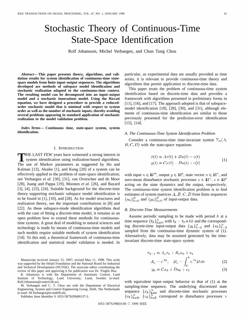
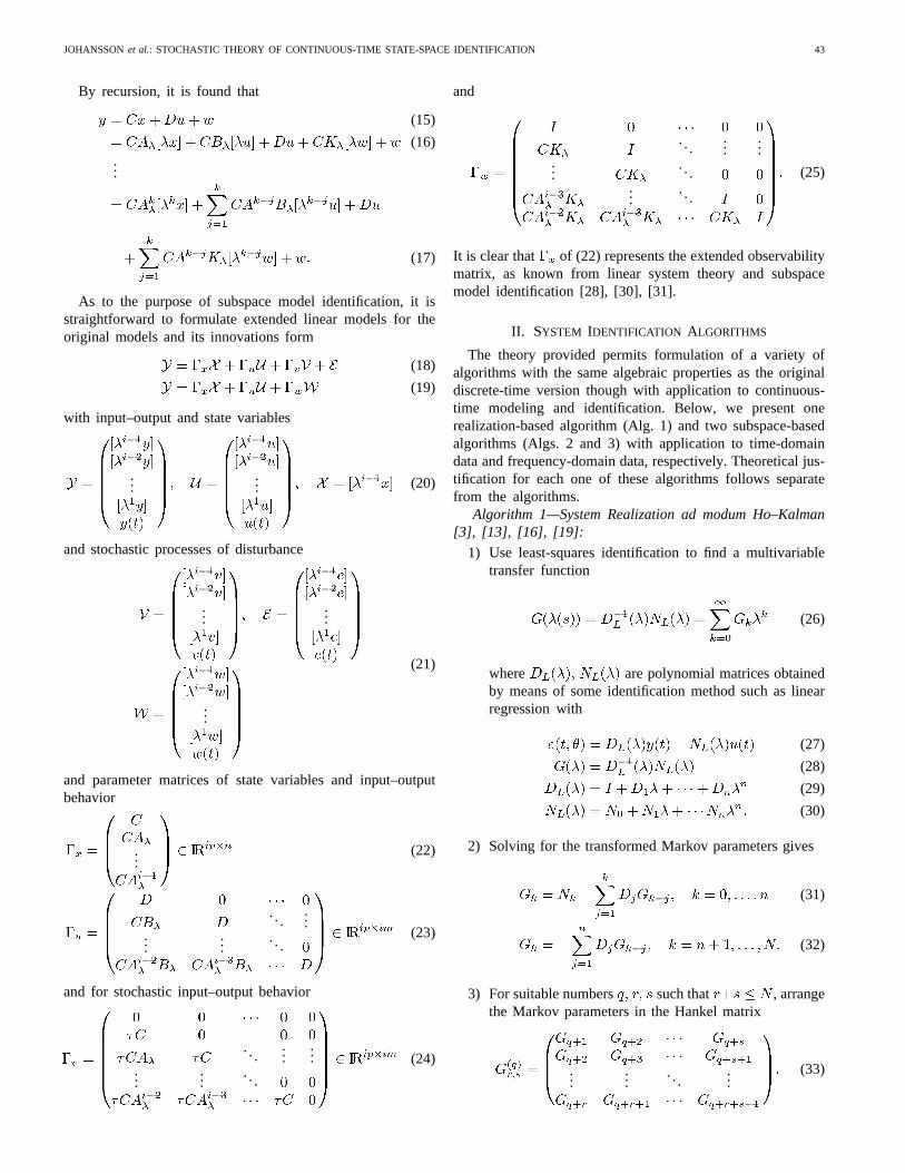
Fig. 1. Autocorrelation functions (upper diagram) and autospectra (diagram below) of a continuous-time (solid line stochastic variablew(t) and a discrete-time(‘o’) sample sequencefwkg. The continuous-time process is bandwidth-limited to the Nyquist frequency!N = �=2 rad/s of a sampling process with samplingfrequency 1 Hz. Properties of the sampled sequencefwkg confirm that the sampled sequence is an uncorrelated stochastic process with a uniform autospectrum.

and , which can be represented by the components

(4)

(5)

with the covariance

rank (6)

Consider a discrete-time time-invariant systemwith the state-space equations with input ,

output , state vector , and noise sequencesacting on the state dynamics and the

output, respectively.Remark: As computation and statistical tests deal with

discrete-time data, we assume the original sampled stochasticdisturbance sequences to be uncorrelated with a uniform spec-trum up to the Nyquist frequency. The underlying continuous-time stochastic processes will have an autocorrelation functionaccording to Fig. 1, thereby avoiding the mathematical prob-lems associated with the stochastic processes of Brownianmotion.

C. Continuous-Time State-Space Linear System

From the set of first-order linear differential equations of(1), we find the Laplace transform

(7)

(8)

Introduction of the complex variable transform

(9)

corresponding to a stable, causal operator permits an algebraictransformation of the model

(10)

(11)

Reformulation while ignoring the initial conditions to linearsystem equations gives

(12)

(13)

the mapping between and being bijective.Provided that a standard positive semi-definiteness conditionof is fulfilled so that the Riccati equation has a solution,it is possible to replace the linear model of (13) with theinnovations model

(14)

JOHANSSONet al.: STOCHASTIC THEORY OF CONTINUOUS-TIME STATE-SPACE IDENTIFICATION 43

By recursion, it is found that

(15)

(16)...

(17)

As to the purpose of subspace model identification, it isstraightforward to formulate extended linear models for theoriginal models and its innovations form

(18)

(19)

with input–output and state variables

...... (20)

and stochastic processes of disturbance

......

...

(21)

and parameter matrices of state variables and input–outputbehavior

...(22)

......

......

. . .(23)

and for stochastic input–output behavior

......

......

.... . .

(24)

and

......

......

.. ....

.. .

(25)

It is clear that of (22) represents the extended observabilitymatrix, as known from linear system theory and subspacemodel identification [28], [30], [31].

II. SYSTEM IDENTIFICATION ALGORITHMS

The theory provided permits formulation of a variety ofalgorithms with the same algebraic properties as the originaldiscrete-time version though with application to continuous-time modeling and identification. Below, we present onerealization-based algorithm (Alg. 1) and two subspace-basedalgorithms (Algs. 2 and 3) with application to time-domaindata and frequency-domain data, respectively. Theoretical jus-tification for each one of these algorithms follows separatefrom the algorithms.

Algorithm 1—System Realization ad modum Ho–Kalman[3], [13], [16], [19]:

1) Use least-squares identification to find a multivariabletransfer function

(26)

where are polynomial matrices obtainedby means of some identification method such as linearregression with

(27)

(28)

(29)

(30)

2) Solving for the transformed Markov parameters gives

(31)

(32)

3) For suitable numbers such that , arrangethe Markov parameters in the Hankel matrix

......

.. ....

(33)

44 IEEE TRANSACTIONS ON SIGNAL PROCESSING, VOL. 47, NO. 1, JANUARY 1999

4) Determine rank and resultant system matrices

(singular value decomposition) (34)

(35)

(36)

(37)

matrix of first columns of (38)

matrix of first columns of (39)

(40)

(41)

(42)

(43)

which yields the th-order state-space realization

(44)

Algorithm 2—Subspace Model Identification (MOESP) [30],[31]:

1) Arrange data matrices by using the followingnotation for sampled filtered data:

etc. (45)

where

......

...

(46)

and a similar construction for .2) Make a QR-factorization such that

(47)

3) Make a SVD of the matrix approximatingthe column space of

(48)

4) Determine estimates of system matrices fromequations

rows through of (49)

rows through of (50)

(51)

rows through of (52)

5) Determine estimate of system matrices fromrelationship

(53)

An algorithmic modification to accommodate frequency-domain data can be made by replacing Step 1 of Algorithm2 by the following.

1 ) Arrange data matrices using the filteredfequency-domain data

(54)

evaluated for

(55)

and arrange a matrix equation of frequency-sampleddata as

......

...

(56)

with similar construction for , and proceed as fromStep 2 of Algorithm 2.

Algorithm 3 (Subspace Correlation Method):Along withthe data matrices of Algorithm 2, introduce thecorrelation variable

......

...

(57)

for chosen sufficiently large. Proceed as fromStep 2 of Algorithm 2 with application of QR factorizationto the matrix

(58)

Theoretical Remarks on the Algorithms:In this section, weprovide some theoretical justification for the algorithms sug-gested:

Algorithm 1—Continuous-Time State-Space Realization:After operator reformulation and a least-squares transferfunction estimate, the algorithm follows the Ho–Kalmanalgorithm step by step.

1) The first step aims toward system identification. The(high-order) least-squares identification serves to find anonminimal input–output model with good prediction-error accuracy as the first priority.

2) Step 2 serves to provide transformed Markov parameterwhere the

(59)

The recursion to obtain may be replaced by alinear equation.

JOHANSSONet al.: STOCHASTIC THEORY OF CONTINUOUS-TIME STATE-SPACE IDENTIFICATION 45

3) Organization of the Markov parameter in the Hankelmatrices of block row dimension and blockcolumn dimension , respectively, permits

(60)

where

...

(61)

Thus, for , the rank of andcannot exceed , which justifies the determination ofmodel order from a rank test of .

4) The last algorithmic step involves a singular valuedecomposition that accomplishes the factorization intothe extended observability matrix and extended control-lability matrix, which permits rank evaluation ofand, hence, estimation of system order. From thefull-rank matrix factors estimates of

and are found. The final transformation toparameter matrices in the-domain provides the state-space realization.

Algorithm 2—Continuous-Time Subspace Model Identifica-tion: This algorithm is similar to the MOESP algorithm ofdiscrete-time subspace model identification.

1) The arrangement of input–output data matricesof sampled data serves to express data the form of (19)so that

(62)

where is the disturbance sample matrix (not avail-able to measurement), and

(63)

2) The QR-factorization serves to retrieve the matrix prod-uct , which is found as the column space ofin the case of disturbance-free data.

3) The singular value factorization of the matrix servesto find the left factor of rank corresponding to(up to a similarity transformation). The rank conditionis evaluated by means of the nonzero singular values of

.4) As the estimate contains products of the -

matrix and powers of , it is straightforward to find anestimate of from the first rows. Next, an estimate

is found. Subsequent transformation of to the-domain is required.

5) Given , then can be found to fit the in-put–output relationship provided by .

Algorithm 2 and its frequency-domain modification arevery closely related as their data matrices with differentinterpretation obey the relationship

(64)

By definition, the discrete-time Fourier transform is formulatedas the linear transformation

......

......

...(65)

For the standard FFT set of frequency points, we have

so that of Algorithm 2 and its frequency-domainversion only differ by a right invertible factor as foundfrom

......

...... (66)

The right factor does not affect the observability subspace,which is always extracted from a left matrix factor and is thequantity of primary interest in subspace model identification.

Algorithm 3—Subspace Correlation Method:The subspacecorrelation method is similar to Algorithm 2 but differs in thelinear dependences

(67)

The left matrix factor extracted in estimation of observabilitysubspace is not affected by the right multiplication of .However, the algorithm output is not identical to that ofAlgorithm 2 due to the change of relative magnitude of thedisturbance term as a result of the right multiplication. Anotherproperty is the reduction of the matrix column dimension ofthe data matrix applied QR-factorization.

When input and disturbance are uncorrelated, this algo-rithm serves to reduce disturbance-related bias in parameterestimates. Statistical properties are analyzed in greater detailbelow.

Example: The algorithms were applied tosamples of input–output data generated by simulation of thelinear system

(68)

(69)

46 IEEE TRANSACTIONS ON SIGNAL PROCESSING, VOL. 47, NO. 1, JANUARY 1999

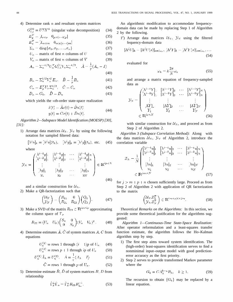
Fig. 2. Input–output data (upper two graphs) and filter data used for identification with sampling periodh = 0:01, filter order i = 5, and operatortime constant� = 0:05.

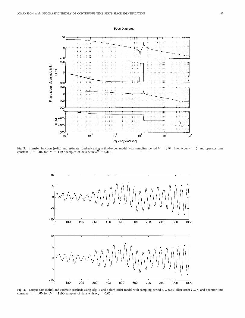
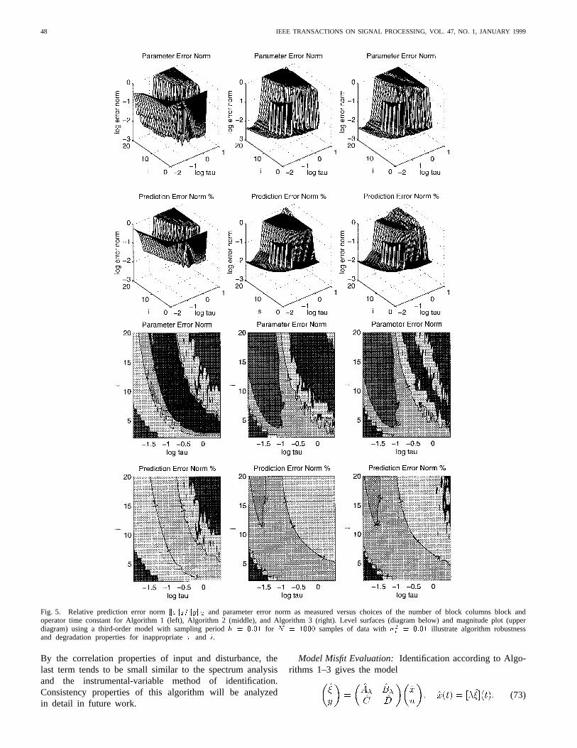
with input of variance and a zero-mean stochasticdisturbance of variance ; see input–output data (Fig. 2).A third-order model was identified with very good accuracyfor purely deterministic data and with good accuracyfor ; see transfer-function properties (Fig. 3) andprediction performance (Fig. 4). The influence of the choicesof algorithmic parameters (number of block rowsorand operator time constant) on relative prediction error

and parameter error as measured by gap metricare found in Fig. 5. The identification was considered to befailing for a relative prediction error norm of value larger thanone. Fig. 5 has been drawn accordingly without representingrelative error larger than one, thus showing the effectiverange of the choice of and . This figure also serves toillustrate sensitivity to stochastic disturbance and sensitivityto the choice of the free algorithm parameters (operator timeconstant and number of block rowsor ). The level surfacesindicate that may be chosen in a suitable range over, perhaps,two orders of magnitude for Algs. 2 and 3 and one order ofmagnitude for Alg. 1; see Fig. 5, which includes contours oflevel surfaces, the central part corresponding to 1% error withdegradation for inappropriate values ofand .

Another application of the realization algorithm (Alg. 1)to experimental impulse-response data obtained as ultrasonicecho data for object identification detection in robotic envi-ronments has proved successful; see [16].

III. STATISTICAL MODEL VALIDATION

Statistical model validation accompanies parameter estima-tion to provide confidence in a model obtained. An important

aspect of statistical model validation is evaluation of themismatch between input–output properties of a model anddata. Statistical hypothesis tests applied to the autocorrelationof residuals as well as cross correlation between residualsand input are instrumental in such model validation, partiallyrelying on the algorithmic property of that

(70)

(71)

where by construction, i.e., by the projectionproperty of the QR-factorization of (47), whereas statisticalproperties of are more difficult to evaluate alsounder assumptions of uncorrelated disturbances and controlinputs. In the case of uncorrelated disturbance and input, mul-tiplication of the right factor before the QR-factorizationin Algorithm 3 serves to reduce the disturbance-related biasof parameter estimates as

(72)

JOHANSSONet al.: STOCHASTIC THEORY OF CONTINUOUS-TIME STATE-SPACE IDENTIFICATION 47

Fig. 3. Transfer function (solid) and estimate (dashed) using a third-order model with sampling periodh = 0:01, filter order i = 5, and operator timeconstant� = 0:05 for N = 1000 samples of data with�2

v= 0:01.

Fig. 4. Output data (solid) and estimate (dashed) using Alg. 2 and a third-order model with sampling periodh = 0:01, filter orderi = 5, and operator timeconstant� = 0:05 for N = 1000 samples of data with�2

v= 0:01.

48 IEEE TRANSACTIONS ON SIGNAL PROCESSING, VOL. 47, NO. 1, JANUARY 1999

Fig. 5. Relative prediction error normk"k2=kyk2 and parameter error norm as measured versus choices of the number of block columns block andoperator time constant for Algorithm 1 (left), Algorithm 2 (middle), and Algorithm 3 (right). Level surfaces (diagram below) and magnitude plot (upperdiagram) using a third-order model with sampling periodh = 0:01 for N = 1000 samples of data with�2

v= 0:01 illustrate algorithm robustness

and degradation properties for inappropriate� and i.

By the correlation properties of input and disturbance, thelast term tends to be small similar to the spectrum analysisand the instrumental-variable method of identification.Consistency properties of this algorithm will be analyzedin detail in future work.

Model Misfit Evaluation: Identification according to Algo-rithms 1–3 gives the model

(73)

JOHANSSONet al.: STOCHASTIC THEORY OF CONTINUOUS-TIME STATE-SPACE IDENTIFICATION 49

A reconstruction of the state for some matrix suchthat is stable, i.e., , can be done as

(74)

Model-error dynamics of and

(75)

The stochastic realization problem can be approached byKalman filter theory and covariance-matrix factorization(“spectral factorization”) [2], [6], and provided that acontinuous-time Riccati equation can be solved to find anoptimal , we find that the model mismatch can be expressedby either of the spectral factors

(76)

(77)

where and are the Laplace trans-forms of the residuals, disturbance, and innovations processes,respectively. The discrete-time counterpart is

(78)

(79)

To solve for identification residuals, it is suitable to use thetransfer operator inverses

(80)

(81)

(82)

For nominal system parameter matrices and asolution and from the Riccati equation ofthe Kalman filter, we would have

(83)

so that the output reproduce of , except for a transientarising from the initial condition of . However, as nocovariance data area priori known and as the system identifi-cation including its validation procedure is assumed to utilizediscrete-time data, it is generally necessary to resort to theresidual realization algorithm

(84)

Reformulation of the Riccati equation (see [9]) is

(85)

where the full-rank matrices arise from the factorization

(86)

and where (85) represents factorization of the covariancematrix of the variables

(87)

(88)

Then, use of the full-rank matrices of (85) suggests thatthe stochastic state-space model be provided as

(89)

with a matrix chosen as the pseudo-inverse ofand with

(90)

An innovations-like model pseudoinverse is provided as

(91)

where are discrete-time versions of and , respec-tively, and with for rank-deficient covariance matrices

replacing the of the standard Kalman filter. Then,the output reproduces the rank-deficient innovationssequence.

IV. DISCUSSION

This paper has treated the problem of continuous-timesystem identification based on discrete-time data and providesa framework with algorithms presented in preliminary formsin [11] and [16], thereby extending subspace model identi-fication to continuous-time models. We have provided bothsubspace-based algorithms and realization-based algorithmswith application both in the time domain and in the frequencydomain. To our knowledge, the time-domain algorithms arethe first algorithms of its kind whereas frequency-domainalgorithms have previously been presented [23], [25]. Severalissues remain open issues, and we cannot claim to have anycomplete treatment. The accuracy of estimates, effects of sto-chastic disturbance, performance comparison and robustnessof algorithms, i.e., algorithmic effects and behavior when datacannot be generated by a model in the model class, needfurther attention; see [28] for discussion on these issues forthe discrete-time case.

A relevant question is, of course, how general is the choiceand if it can, for instance, be replaced by some other bijectivemapping

(92)

50 IEEE TRANSACTIONS ON SIGNAL PROCESSING, VOL. 47, NO. 1, JANUARY 1999

with the Laplace-transformed linear model

(93)

and by the operator transformation shown at the top of thepage. Obviously, such an operator transformation entails anonlinear parameter transformation with an inverse

(94)

which, of course, may be error prone or otherwise sensitivedue to singularities or poor numerical properties of the matrixinverse. By comparison, a model transformation usingislinear, simple, and does not exhibit such parameter-matrix sin-gularities: a circumstance that motivates the attention given thefavorable properties of this transformation. Actually, furtherstudies to cover other linear fractional transformations are inprogress [11], including advice on the choice of the additionalparameters involved.

We have considered the problem of finding appropriatestochastic realization to accompany estimated input–outputmodels in the case of multi-input multioutput subspace modelidentification. The case considered includes the problem ofrank-deficient residual covariance matrices: a case that is en-countered in applications with mixed stochastic-deterministicinput–output properties as well as for cases where outputs arelinearly dependent [28]. The inverse of output covariance ma-trix is generally needed both for formulation of an innovationsmodel and for a Kalman filter [18], [27], [29]. Our approachhas been the formulation of an innovations model for therank-deficient model output that generalizes previously usedmethods of stochastic realization [5], [7], [21], [22].

The modified pseudoinverse of (91) provides the meansto evaluate a residual sequence from the mismatch betweenan identified continuous-time model and discrete-time datain such a way that standard statistical validation test can beapplied [14]. Such statistical tests include the following:

• autocorrelation test of residual sequence ;• cross correlation test of input and residual sequence

;• test of normal distribution (zero crossings, distribution,

skewness, kurtosis, etc.).

V. CONCLUSION

This paper has treated the problem of continuous-timesystem identification based on discrete-time data and providesa framework with algorithms presented in preliminary formsin [11] and [16]. The methodology involves a continuous-time operator translation [14], [15], permitting an algebraicreformulation and the use of subspace and realization algo-rithms. We have provided subspace-based algorithms as well

as realization-based algorithms with application both to timedomain and to frequency-domain data. Thus, the algorithmsand the theory presented here provide extensions both ofthe continuous-time identification and of subspace modelidentification.

A favorable property is the following. Whereas the modelobtained is a continuous-time model, statistical tests canproceed in a manner that is standard for discrete-time models[14]. Conversely, as validation data are generally availableas discrete-time data, it is desirable to provide means forvalidation of continuous-time models to available data.

REFERENCES

[1] H. Akaike, “Markovian representation of stochastic processes by canon-ical variables,”SIAM J. Contr., vol. 13, pp. 162–173, 1975.

[2] B. D. O. Anderson and P. J. Moylan, “Spectral factorization of a finite-dimensional nonstationary matrix covariance,”IEEE Trans. Automat.Contr., vol. AC-19, pp. 680–692, 1974.

[3] D. S. Bayard, “An algorithm for state-space frequency domain identi-fication without windowing distortions,”IEEE Trans. Automat. Contr.,vol. 39, pp. 1880–1885, Sept. 1994.

[4] S. Bigi, T. Soderstrom, and B. Carlsson, “An IV-scheme for estimatingcontinuous-time stochastic models from discrete-time data,” inProc.IFAC SYSID, Copenhagen, Denmark, 1994, vol. 3, pp. 645–650.

[5] U. B. Desai and D. Pal, “A realization approach to stochastic modelreduction and balanced stochastic realizations,” inProc. IEEE Conf.Decision Contr., Orlando, FL, 1982, pp. 1105–1112.

[6] B. W. Dickinson, T. Kailath, and M. Morf, “Canonical matrix frac-tion and state-space description for deterministic and stochastic linearsystems,”IEEE Trans. Automat. Contr., vol. AC-19, pp. 656–667, 1974.

[7] P. Faurre, “Stochastic realization algorithms,” inSystem Identification:Advances and Case Studies, R. K. Mehra and D. Lainiotis, Eds. NewYork: Academic, 1976.

[8] R. Guidorzi, “Canonical structures in the identification of multivariablesystems,”Automatica, vol. 11, pp. 361–374, 1975.

[9] P. Hagander and A. Hansson, “How to solve singular discrete-timeRiccati equations,” inProc. IFAC, Preprints 13th IFAC World Congr.,San Francisco, CA, July 1996, pp. 313–318.

[10] E. J. Hannan and M. Deistler,The Statistical Theory of Linear Systems.New York: Wiley, 1988.

[11] B. R. J. Haverkamp, C. T. Chou, M. Verhaegen, and R. Johansson,“Identification of continuous-time MIMO state space models fromsampled data, in the presence of process and measurement noise,”in Proc. IEEE Conf. Decision Contr., Kobe, Japan, Dec. 1996, pp.1539–1544.

[12] B. R. J. Haverkamp, M. Verhaegen, C. T. Chou, and R. Johansson,“Continuous-time identification of MIMO state-space models from sam-pled data,” inProc. 11th IFAC Symp. System Ident. (SYSID), Kitakyushu,Japan, 1997.

[13] B. L. Ho and R. E. Kalman, “Effective construction of linear state-variable models from input/output functions,”Regelungstechnik, vol.14, pp. 545–548, 1966.

[14] R. Johansson,System Modeling and Identification. Englewood Cliffs,NJ: Prentice-Hall, 1993.

[15] , “Identification of continuous-time models,”IEEE Trans. SignalProcessing, vol. 42, pp. 887–897, Apr. 1994.

[16] R. Johansson and G. Lindstedt, “An algorithm for continuous-time statespace identification, inProc. 34th IEEE Conf. Decision and Control,New Orleans, LA, 1995, pp. 721–722.

[17] R. Johansson, M. Verhaegen, and C. T. Chou, “Stochastic theoryof continuous-time state-space identification,” inProc. Conf. DecisionContr., San Diego, CA, 1997, pp. 1866–1871.

JOHANSSONet al.: STOCHASTIC THEORY OF CONTINUOUS-TIME STATE-SPACE IDENTIFICATION 51

[18] J. N. Juang,Applied System Identification. Englewood Cliffs, NJ:Prentice-Hall, 1994.

[19] J. N. Juang and R. S. Pappa, “An eigensystem realization algorithmfor modal parameter identification and model reduction,”J. Guidance,Contr. Dyn., vol. 8, pp. 620–627, 1985.

[20] S. Y. Kung, “A new identification and model reduction algorithm viasingular value decomposition,” inProc. 12th Asilomar Conf. Circuits,Syst. Comput., Pacific Grove, CA, 1978, pp. 705–714.

[21] W. Larimore, “Canonical variate analysis in identification, filtering andadaptive control,” inProc. 29th IEEE Conf. Decision Contr., 1990, pp.596–604.

[22] A. Lindquist and G. Picci, “Realization theory for multivariate stationaryGaussian processes,”SIAM J. Contr. Optimiz., vol. 23, no. 6, pp.809–857, 1985.

[23] T. McKelvey and H. Akcay, “An efficient frequency domain state-spaceidentification algorithm,” inProc. 33rd IEEE Conf. Decision Contr.,1994, pp. 3359–3364.

[24] , “An efficient frequency domain state-space identification algo-rithm: Robustness and stochastic analysis,” inProc. 33rd IEEE Conf.Decision Contr., 1994, pp. 3348–3353.

[25] T. McKelvey, H. Akcay, and L. Ljung, “Subspace-based multivari-able system identification from frequence response data,”IEEE Trans.Automat. Contr., vol. 41, pp. 960–979, 1996.

[26] M. Moonen, B. D. Moor, L. Vandenberghe, and J. Vandewalle, “On andoff-line identification of linear state-space models,”Int. J. Contr., vol.49, pp. 219–232, 1989.

[27] P. Van Overschee and B. De Moor, “N4SID: Subspace algorithmfor the identification of combined deterministic-stochastic systems,”Automatica, vol. 30, pp. 75–93, 1994.

[28] P. V. Overschee and B. D. Moor,Subspace Identification for LinearSystems—Theory, Implementation, ApplicationsBoston, MA: Kluwer,1996.

[29] M. Verhaegen, “Identification of the deterministic part of MIMO statespace models given in innovation form from input-output data,”Auto-matica, Special Issue on Statistical Signal Processing and Control, vol.30, no. 1, pp. 61–74, 1994.

[30] M. Verhaegen and P. Dewilde, “Subspace model identifica-tion—Analysis of the elementary output-error state-space modelidentification algorithm,”Int. J. Contr., vol. 56, pp. 1211–1241, 1992.

[31] , “Subspace model identification—The output-error state-spacemodel identifications class of algorithms,”Int. J. Contr., vol. 56, pp.1187–1210, 1992.

Rolf Johanssonreceived the M.S. degree in tech-nical physics in 1977, the B.M. degree in 1980, andthe Ph.D. degree in 1983 (control theory). He wasappointed Docent in 1985 and received the M.D.degree from Lund University, Lund, Sweden, in1986.

Since 1986, he has been an Associate Professor ofControl Theory at the Lund Institute of Technology,Lund University, with side appointments on theFaculty of Medicine. Currently, he is CoordinatingDirector of Robotics Research with participants

from several departments of Lund University. He has had visiting appoint-ments at Laboratoire d’Automatique de Grenoble, Grenoble, France, theCalifornia Institute of Technology, Pasadena, and Rice University, Houston,TX. In his scientific work, he has been involved in research in adaptivesystem theory, mathematical modeling, system identification, robotics, signalprocessing theory, and biomedical research. He is the author of the bookSystem Modeling and Identification(Englewood Cliffs, NJ: Prentice-Hall,1993).

Dr. Johansson was awarded the biomedical engineering prize (the EbelingPrize) of the Swedish Society of Medicine in 1995.

Michel Verhaegen received the B.S. degree inengineering/aeronautics from the Delft University ofTechnology, Delft, The Netherlands, in August 1982and the Ph.D. degree in applied sciences from theCatholic University Leuven, Leuven, Belgium, inNovember 1985. During his graduate study, he heldan IWONL research assistantship in the Departmentof Electrical Engineering.

From 1985 to 1987, he was a Postdoctoral As-sociate of the U.S. National Research Council, andduring that time, he was affiliated with the NASA

Ames Research Center, Mountain View, CA. From 1988 to 1989, he wasan Assistant Professor at the Department of Electrical Engineering, DelftUniversity of Technology. Since February 1990, he has been a Senior ResearchFellow of the Dutch Academy of Arts and Sciences and has also been affiliatedwith the Network Theory Group, Delft University of Technology. Since 1990,he has held short sabbatical leaves at the University of Uppsala, Uppsala,Sweden, McGill Unversity, Montreal, P.Q., Canada, Lund University, Lund,Sweden, and the German Aerospace Research Center (DLR), Munich. Cur-rently, he is an Associate Professor with the Delft University of Technologyand is head of the Systems and Control Engineering Group of the Facultyof Information Technology and Systems. His main research interest is theinterdisciplinary domain of numerical algebra and system theory. In this field,he has published over 100 papers. Current activities focus on the developmentand practical application of new identification and simulation tools in model-based industrial controller design.

Dr. Verhaegen received a Best Presentation Award at the American ControlConference, Seattle, WA, in 1986 and a Recognition Award from NASA in1989. He is project leader of a number of research projects sponsored by theEuropean Community, the Dutch National Science Foundation (STW), andthe Delft University of Technology.

Chun Tung Chou was born in Hong Kong in1967. He received the B.A. degree in engineeringscience from Oxford University, Oxford, U.K., in1988 and the Ph.D. degree in control engineeringfrom University of Cambridge, Cambridge, U.K.,in 1994.

He is currently a Post-Doctoral Research Fellowwith the Electrical Engineering Department, DelftUniversity of Technology, Delft, The Netherlands.His current research interests are system identifica-tion of linear and nonlinear systems.