Embed Size (px)
Citation preview
Discrete and continuous stochastic modelling
Grant Lythe
Applied Mathematics, University of Leeds, UK
Some useful books are Stirzaker Stochastic processes and modelsTaylor and Karlin An Introduction to Stochastic Modelling
Linda Allen An introduction to stochastic processes with applications to biology
2009
Grant Lythe (Leeds, UK) Stochastic modelling 2009 1 / 25
Summary
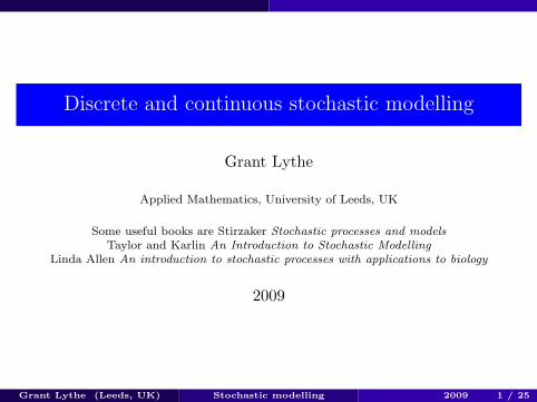
1 Markov processes: the Gillespie algorithmIntroduction: Gambler’s ruinContinuous-time Markov chainsThe Gillespie algorithm
2 Stochastic processes in continuous spaceBrownian motion or the Wiener processA bit of immunology
3 T-cell homeostasis
Grant Lythe (Leeds, UK) Stochastic modelling 2009 2 / 25
Markov processes: the Gillespie algorithm Introduction: Gambler’s ruin
Gambler’s ruin: The rules of the game
A gambler tosses a fair coin. Each time the coin lands heads, thegambler gains a dollar and each time the coin lands tails, the gamblerloses a dollar. The game continues until the gambler either loses Bdollars (is ruined) or wins A dollars (wins overall).
Let Sn be the net winnings after n tosses. Suppose S0 = k. Let τ bethe number of steps it takes to end the game. Iff(k) = Pr[hit A before −B] and g(k) = IE(τ)then f(k) = 1
2f(k − 1) + 12f(k + 1)
and g(k) = 12g(k − 1) + 1
2g(k + 1) + 1.
Grant Lythe (Leeds, UK) Stochastic modelling 2009 3 / 25
Markov processes: the Gillespie algorithm Continuous-time Markov chains
Continuous-time Markov chains
If time is now a continuous variable then we define the transitionprobability function as
Pij(t + u) = Pr[Xt+u = j|Xu = i] t ≥ 0.
Now t ∈ IR+ but i and j are still integers.If the Pij(t + u) do not depend on u, we say the Markov chain hasstationary transition probabilities.
Grant Lythe (Leeds, UK) Stochastic modelling 2009 4 / 25
Markov processes: the Gillespie algorithm Continuous-time Markov chains
Birth processes
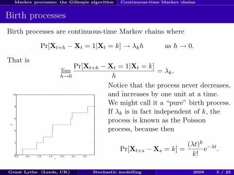
Birth processes are continuous-time Markov chains where
Pr[Xt+h −Xt = 1|Xt = k] → λkh as h → 0.
That islimh→0
Pr[Xt+h −Xt = 1|Xt = k]h
= λk.
0.0 0.5 1.0 1.5 2.0 2.5 3.0t
0
2
4
6
8
10
X
Notice that the process never decreases,and increases by one unit at a time.We might call it a “pure” birth process.If λk is in fact independent of k, theprocess is known as the Poissonprocess, because then
Pr[Xt+s −Xs = k] =(λt)k
k!e−λt.
Grant Lythe (Leeds, UK) Stochastic modelling 2009 5 / 25
Markov processes: the Gillespie algorithm Continuous-time Markov chains
Time of the first jump
If τ is the time of the first jump, then
ddt
Pr[τ > t] = −λPr[τ > t]
and Pr[τ > 0] = 1. Thus
Pr[τ > t] = exp (−λt) .
Grant Lythe (Leeds, UK) Stochastic modelling 2009 6 / 25
Markov processes: the Gillespie algorithm The Gillespie algorithm
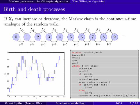
Birth and death processes
If Xt can increase or decrease, the Markov chain is the continuous-timeanalogue of the random walk.
0 1 2 3 4 5 6 7 8 9 · · ·µ1 µ2 µ3 µ4 µ5 µ6 µ7 µ8 µ9
λ0 λ1 λ2 λ3 λ4 λ5 λ6 λ7 λ8
0 5 10 15 20 25 30 35 40 45t
10
12
14
16
18
20
22
Xt
i m p o r t random , m a t ht m a x=100x0=10t=0x=x0
w h i l e t <= t m a x :l a m b =1.0mu=2.0i f x==0:
mu=0r a t e=l a m b+mu
urv=r a n d o m . r a n d o m ( )i f urv>=l a m b / r a t e :
x−=1e l s e :
x+=1t+=−m a t h . log ( r a n d o m . r a n d o m ( ) ) / r a t e
Grant Lythe (Leeds, UK) Stochastic modelling 2009 7 / 25
Markov processes: the Gillespie algorithm The Gillespie algorithm
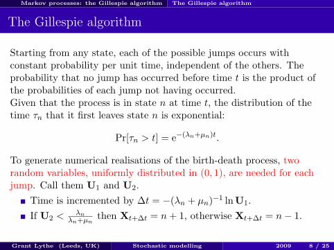
The Gillespie algorithm
Starting from any state, each of the possible jumps occurs withconstant probability per unit time, independent of the others. Theprobability that no jump has occurred before time t is the product ofthe probabilities of each jump not having occurred.Given that the process is in state n at time t, the distribution of thetime τn that it first leaves state n is exponential:
Pr[τn > t] = e−(λn+µn)t.
To generate numerical realisations of the birth-death process, tworandom variables, uniformly distributed in (0, 1), are needed for eachjump. Call them U1 and U2.
Time is incremented by ∆t = −(λn + µn)−1 lnU1.If U2 < λn
λn+µnthen Xt+∆t = n + 1, otherwise Xt+∆t = n− 1.
Grant Lythe (Leeds, UK) Stochastic modelling 2009 8 / 25
Markov processes: the Gillespie algorithm The Gillespie algorithm
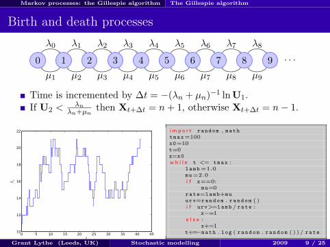
Birth and death processes
0 1 2 3 4 5 6 7 8 9 · · ·µ1 µ2 µ3 µ4 µ5 µ6 µ7 µ8 µ9
λ0 λ1 λ2 λ3 λ4 λ5 λ6 λ7 λ8
Time is incremented by ∆t = −(λn + µn)−1 lnU1.If U2 < λn
λn+µnthen Xt+∆t = n + 1, otherwise Xt+∆t = n− 1.
0 5 10 15 20 25 30 35 40 45t
10
12
14
16
18
20
22
Xt
i m p o r t random , m a t ht m a x=100x0=10t=0x=x0
w h i l e t <= t m a x :l a m b =1.0mu=2.0i f x==0:
mu=0r a t e=l a m b+mu
urv=r a n d o m . r a n d o m ( )i f urv>=l a m b / r a t e :
x−=1e l s e :
x+=1t+=−m a t h . log ( r a n d o m . r a n d o m ( ) ) / r a t e
Grant Lythe (Leeds, UK) Stochastic modelling 2009 9 / 25
Markov processes: the Gillespie algorithm The Gillespie algorithm
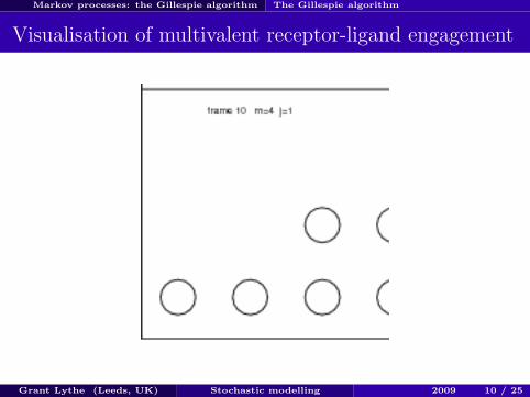
Visualisation of multivalent receptor-ligand engagement
Grant Lythe (Leeds, UK) Stochastic modelling 2009 10 / 25
Stochastic processes in continuous space
1 Markov processes: the Gillespie algorithmIntroduction: Gambler’s ruinContinuous-time Markov chainsThe Gillespie algorithm
2 Stochastic processes in continuous spaceBrownian motion or the Wiener processA bit of immunology
3 T-cell homeostasis
Grant Lythe (Leeds, UK) Stochastic modelling 2009 11 / 25

Stochastic processes in continuous space
Stochastic processes
A stochastic process X is a series of random variables labelled bytime.The value of the process at time t is a random variable that wewrite Xt.When time is continuous (t is a real number) we say that X is acontinuous-time stochastic process.One realization of a stochastic process is a sample path. When wecan draw these paths without lifting the pen from the paper, wesay that the stochastic process has continuous paths.
Grant Lythe (Leeds, UK) Stochastic modelling 2009 12 / 25
Stochastic processes in continuous space Brownian motion or the Wiener process
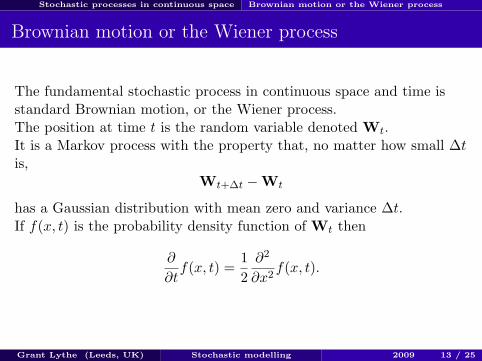
Brownian motion or the Wiener process
The fundamental stochastic process in continuous space and time isstandard Brownian motion, or the Wiener process.The position at time t is the random variable denoted Wt.It is a Markov process with the property that, no matter how small ∆tis,
Wt+∆t −Wt
has a Gaussian distribution with mean zero and variance ∆t.If f(x, t) is the probability density function of Wt then
∂
∂tf(x, t) =
12
∂2
∂x2f(x, t).
Grant Lythe (Leeds, UK) Stochastic modelling 2009 13 / 25
Stochastic processes in continuous space Brownian motion or the Wiener process
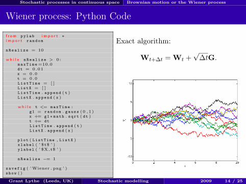
Wiener process: Python Code
f r om p y l a b i m p o r t ∗i m p o r t r a n d o m
n R e a l i z e = 10
w h i l e n R e a l i z e > 0 :m a x T i m e =10.0dt = 0.01x = 0.0t = 0.0L i s t T i m e = [ ]L i s t X = [ ]L i s t T i m e . a p p e n d ( t )L i s t X . a p p e n d ( x )
w h i l e t <= m a x T i m e :g1 = r a n d o m . g a u s s (0 , 1 )x += g1∗ m a t h . s q r t ( dt )t += dt
L i s t T i m e . a p p e n d ( t )L i s t X . a p p e n d ( x )
p l o t ( L i s t T i m e , L i s t X )x l a b e l ( ’ $t$ ’ )y l a b e l ( ’ $X t$ ’ )
n R e a l i z e −= 1
s a v e f i g ( ’ Wiener . png ’ )s h o w ( )
Exact algorithm:
Wt+∆t = Wt +√
∆tG.
Grant Lythe (Leeds, UK) Stochastic modelling 2009 14 / 25
Stochastic processes in continuous space Brownian motion or the Wiener process
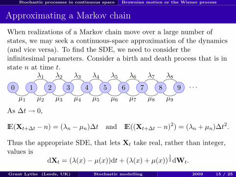
Approximating a Markov chain
When realizations of a Markov chain move over a large number ofstates, we may seek a continuous-space approximation of the dynamics(and vice versa). To find the SDE, we need to consider theinfinitesimal parameters. Consider a birth and death process that is instate n at time t.
0 1 2 3 4 5 6 7 8 9 · · ·µ1 µ2 µ3 µ4 µ5 µ6 µ7 µ8 µ9
λ1 λ2 λ3 λ4 λ5 λ6 λ7 λ8
As ∆t → 0,
IE(Xt+∆t − n) = (λn − µn)∆t and IE((Xt+∆t − n)2) = (λn + µn)∆t2.
Thus the appropriate SDE, that lets Xt take real, rather than integer,values is
dXt = (λ(x)− µ(x))dt + (λ(x) + µ(x))12 dWt.
Grant Lythe (Leeds, UK) Stochastic modelling 2009 15 / 25
Stochastic processes in continuous space A bit of immunology
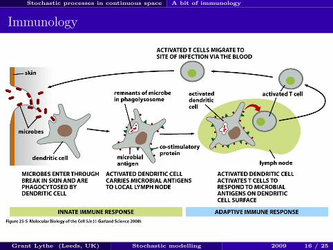
Immunology
Grant Lythe (Leeds, UK) Stochastic modelling 2009 16 / 25
Stochastic processes in continuous space A bit of immunology
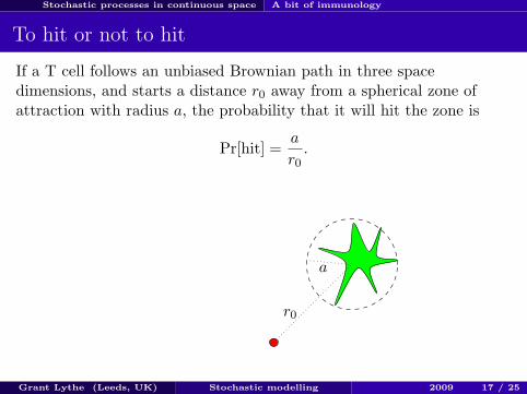
To hit or not to hit
If a T cell follows an unbiased Brownian path in three spacedimensions, and starts a distance r0 away from a spherical zone ofattraction with radius a, the probability that it will hit the zone is
Pr[hit] =a
r0.
r0
a
Grant Lythe (Leeds, UK) Stochastic modelling 2009 17 / 25
Stochastic processes in continuous space A bit of immunology
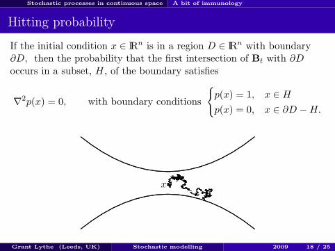
Hitting probability
If the initial condition x ∈ IRn is in a region D ∈ IRn with boundary∂D, then the probability that the first intersection of Bt with ∂Doccurs in a subset, H, of the boundary satisfies
∇2p(x) = 0, with boundary conditions
{p(x) = 1, x ∈ H
p(x) = 0, x ∈ ∂D −H.
.....................
........................
...........................................
..........................................
........................................
.......................................
...................................... ..................................... .................................... .................................... ...........................................................................
...............................................................................
..........................................
...........................................
............................................
.............................................
...........................................
..........................................
...............................................................................
........................................................................... .................................... .................................... ..................................... ......................................
.......................................
........................................
..........................................
...........................................
........................................
....
x
Grant Lythe (Leeds, UK) Stochastic modelling 2009 18 / 25
Stochastic processes in continuous space A bit of immunology
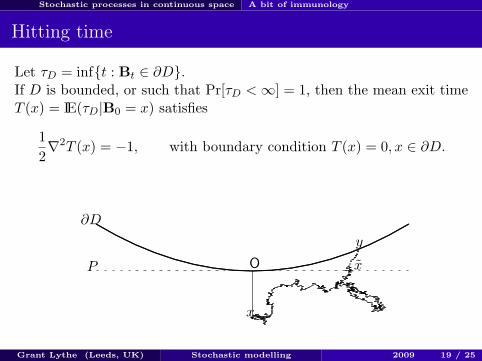
Hitting time
Let τD = inf{t : Bt ∈ ∂D}.If D is bounded, or such that Pr[τD < ∞] = 1, then the mean exit timeT (x) = IE(τD|B0 = x) satisfies
12∇2T (x) = −1, with boundary condition T (x) = 0, x ∈ ∂D.
...........................
..........................
...................................................
..................................................
.................................................
................................................ ............................................... ............................................. ............................................ ............................................ ............................................................................................
.................................................................................................
..................................................
...................................................
....................................................
P
∂D
qxO ax̃y
Grant Lythe (Leeds, UK) Stochastic modelling 2009 19 / 25
Stochastic processes in continuous space A bit of immunology
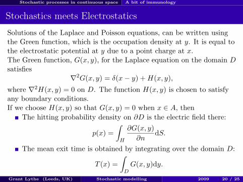
Stochastics meets Electrostatics
Solutions of the Laplace and Poisson equations, can be written usingthe Green function, which is the occupation density at y. It is equal tothe electrostatic potential at y due to a point charge at x.The Green function, G(x, y), for the Laplace equation on the domain Dsatisfies
∇2G(x, y) = δ(x− y) + H(x, y),
where ∇2H(x, y) = 0 on D. The function H(x, y) is chosen to satisfyany boundary conditions.If we choose H(x, y) so that G(x, y) = 0 when x ∈ A, then
The hitting probability density on ∂D is the electric field there:
p(x) =∫
H
∂G(x, y)∂n
dS.
The mean exit time is obtained by integrating over the domain D:
T (x) =∫
DG(x, y)dy.
Grant Lythe (Leeds, UK) Stochastic modelling 2009 20 / 25

Stochastic processes in continuous space A bit of immunology
Finding the way out
If the cell is reflected everywhere except for a “polar cap” exit with
radius a, then the mean time to escape isπ
3R3
Da.
θe
The time to hit an exit, that makes an angle θe,on the surface of a sphere is given by solvingLaplace’s equation:
∇2τ =1r2
∂
∂r
(r2 ∂τ
∂r
)+
1r2 sin θ
∂
∂θ
(sin θ
∂τ
∂θ
)= −D,
with boundary conditions;
τ(R, θ) = 0 if 0 ≤ θ < θe
∂τ
∂r= 0 if θe ≤ θ ≤ π.
Grant Lythe (Leeds, UK) Stochastic modelling 2009 21 / 25
Stochastic processes in continuous space A bit of immunology
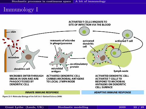
Immunology I
Grant Lythe (Leeds, UK) Stochastic modelling 2009 22 / 25
T-cell homeostasis
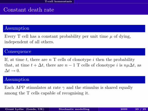
Constant death rate
Assumption
Every T cell has a constant probability per unit time µ of dying,independent of all others.
Consequence
If, at time t, there are n T cells of clonotype i then the probabilitythat, at time t + ∆t, there are n− 1 T cells of clonotype i is nµ∆t, as∆t → 0.
Assumption
Each APP stimulates at rate γ and the stimulus is shared equallyamong the T cells capable of recognising it.
Grant Lythe (Leeds, UK) Stochastic modelling 2009 23 / 25
T-cell homeostasis
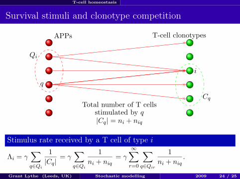
Survival stimuli and clonotype competition
APPs T-cell clonotypes
q
i
Cq
Qi
Total number of T cellsstimulated by q|Cq| = ni + niq
Stimulus rate received by a T cell of type i
Λi = γ∑q∈Qi
1|Cq|
= γ∑q∈Qi
1ni + niq
= γ
∞∑r=0
∑q∈Qir
1ni + niq
.
Grant Lythe (Leeds, UK) Stochastic modelling 2009 24 / 25
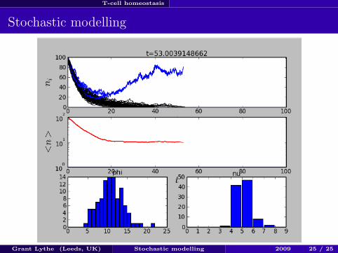
T-cell homeostasis
Stochastic modelling
Grant Lythe (Leeds, UK) Stochastic modelling 2009 25 / 25


![[Geoffrey Grimmett, David Stirzaker] One Thousand (BookZZ.org)](https://img.pdfslide.us/doc/110x75/55cf882a55034664618e0afa/geoffrey-grimmett-david-stirzaker-one-thousand-bookzzorg.jpg)