Embed Size (px)
Citation preview
STOCHAST IC TERM STRUCTURE MODEL ING
An empirical performance analysis of the Lévy Forward Price Model
MSc in Econometrics
robert verschuren10642447
A Master’s Thesis to obtain the degree in
financial econometrics
In collaboration with
Supervisor: Prof. Dr. C.G.H. Diks
In-company supervisor: Ir. Drs. B.J.W. Kobus
Second reader: Dr. S.A. Broda
July 13, 2017 – Final draft
Faculty of Economics and BusinessAmsterdam School of Economics
Requirements thesis MSc in Econometrics.
1. The thesis should have the nature of a scientic paper. Consequently the thesis is dividedup into a number of sections and contains references. An outline can be something like (thisis an example for an empirical thesis, for a theoretical thesis have a look at a relevant paperfrom the literature):
(a) Front page (requirements see below)
(b) Statement of originality (compulsary, separate page)
(c) Introduction
(d) Theoretical background
(e) Model
(f) Data
(g) Empirical Analysis
(h) Conclusions
(i) References (compulsary)
If preferred you can change the number and order of the sections (but the order youuse should be logical) and the heading of the sections. You have a free choice how tolist your references but be consistent. References in the text should contain the namesof the authors and the year of publication. E.g. Heckman and McFadden (2013). Inthe case of three or more authors: list all names and year of publication in case of therst reference and use the rst name and et al and year of publication for the otherreferences. Provide page numbers.
2. As a guideline, the thesis usually contains 25-40 pages using a normal page format. All thatactually matters is that your supervisor agrees with your thesis.
3. The front page should contain:
(a) The logo of the UvA, a reference to the Amsterdam School of Economics and the Facultyas in the heading of this document. This combination is provided on Blackboard (inMSc Econometrics Theses & Presentations).
(b) The title of the thesis
(c) Your name and student number
(d) Date of submission nal version
(e) MSc in Econometrics
(f) Your track of the MSc in Econometrics
1

Statement of Originality
This document is written by Student Robert Verschuren who declaresto take full responsibility for the contents of this document. I declarethat the text and the work presented in this document is original andthat no sources other than those mentioned in the text and its referenceshave been used in creating it. The Faculty of Economics and Business isresponsible solely for the supervision of completion of the work, not forthe contents.

ABSTRACT
In this thesis we explore how we can best construct and estimate astochastic term structure model for Asset Liability Management purposes.To achieve this, we present an overview of state-of-the-art stochastic inter-est rate models and compare the resulting term structure models in termsof various model criteria. As a result, we adopt the Lévy Forward PriceModel of Eberlein and Özkan (2005) with four different deterministicvolatility specifications under a piecewise homogeneity restriction. Afterintroducing a novel parameterization of this restriction with both deter-ministic and random breakpoints, we adopt a stripping procedure andthe bootstrap method to obtain the market prices of interest rate capletsthrough Bloomberg. We perform a comparative analysis of the empiricalperformance of these eight model extensions by assessing their goodness-of-fit, their parameter stability and their out-of-sample pricing perfor-mance. We calibrate these model extensions under the Normal InverseGaussian distribution by approximating the analytical pricing formulaof Eberlein et al. (2016) for an interest rate caplet with the trapezoidalmethod. We conclude that the Linear-Exponential Volatility specificationis superior to the other model extensions and that it is best to includedeterministic, rather than random breakpoints in the Lévy Forward PriceModel.
Keywords: Stochastic term structures, negative interest rates, determin-istic volatility, piecewise homogeneity, interest rate caplets, calibration.
iii


CONTENTS
1 introduction 12 stochastic term structure models 5
2.1 Previous studies . . . . . . . . . . . . . . . . . . . . . . . 52.2 Model selection . . . . . . . . . . . . . . . . . . . . . . . . 82.3 Extensions of the model . . . . . . . . . . . . . . . . . . . 10
2.3.1 Deterministic volatility specifications . . . . . . . . 102.3.2 Resolving the curse of dimensionality . . . . . . . . 11
2.4 Model performance criteria . . . . . . . . . . . . . . . . . 123 lévy forward price model 15
3.1 Model specification . . . . . . . . . . . . . . . . . . . . . . 153.1.1 Underlying assumptions . . . . . . . . . . . . . . . 163.1.2 Construction of the forward price process . . . . . 173.1.3 Summary of the model . . . . . . . . . . . . . . . . 20
3.2 Piecewise homogeneity . . . . . . . . . . . . . . . . . . . . 223.3 Pricing interest rate caps . . . . . . . . . . . . . . . . . . 24
4 data and optimization routines 274.1 Financial market data . . . . . . . . . . . . . . . . . . . . 27
4.1.1 Bootstrap-implied discount factors . . . . . . . . . 284.1.2 Stripping caplet quotes from cap quotes . . . . . . 31
4.2 Optimization schemes . . . . . . . . . . . . . . . . . . . . 365 empirical performance analysis 39
5.1 Goodness-of-fit . . . . . . . . . . . . . . . . . . . . . . . . 395.2 Parameter stability . . . . . . . . . . . . . . . . . . . . . . 435.3 Out-of-sample pricing . . . . . . . . . . . . . . . . . . . . 46
6 summary and concluding remarks 51references 55
a historical market data 59b additional figures and tables 67
v


1INTRODUCTION
Over the last decade, risk management practices have become increas-ingly emphasized in the financial sector and have in fact become inter-twined with adequate day-to-day management of financial institutions. Ittherefore comes as no surprise that financial institutions are, nowadays,more and more obliged to report the risks they face. One of the key areaswhere financial institutions are liable to high levels of risk and that hasreceived a surge of attention recently, is interest rate risk management.Barely four months ago, the European Central Bank (ECB), for instance,published the details of the sensitivity analysis of interest rate risk in thebanking book (IRRBB) in their annual supervisory stress test for 2017,where the occurrence of negative interest rates is apparent.
Figure 1. ECB sensitivity analysis of IRRBB - stress test 2017. As-sumptions for changes in the interest rate environment in the ECB’s annualsupervisory stress test for 2017. Source: https://www.bankingsupervision.europa.eu/about/ssmexplained/html/2017_stress_test_FAQ.en.html.
We can see from Figure 1, for example, that this annual stress test iscomprised of various scenarios for changes in the interest rate environ-ment, where we not only observe a flat, a decreasing, or an increasing
1

2 introduction
term structure, but a humped and an inversely humped term structureas well. The assumptions underlying this stress test illustrate the im-portance and the significance of the negative interest rate environmentthat we currently observe in the market, and of the consequences of suchnegative rates for financial institutions.The fact that particularly this area of risk management has drawn
so much attention lately, is due to the serious risk that this low, neg-ative interest rate environment poses for financial institutions. Finan-cial institutions that are especially prone to this type of risk are thosewith a duration-mismatch between assets and liabilities. In the case of aduration-mismatch, the liabilities of a financial institution have a longertime to maturity than the opposing assets, which is typically the casefor pension funds and insurance companies. This basically means that adecrease in the term structure of interest rates will lead to an increasein the present value of long-term liabilities, accompanied by a lesser in-crease in the present value of short-term assets. It therefore makes sensethat financial institutions, and especially pension funds and insurancecompanies, adequately take this interest rate risk into account. One wayfor financial institutions to address these issues is by implementing thefindings of an Asset Liability Management (ALM) study.An ALM study is one of the tools that financial institutions can em-
ploy to gain a deeper insight into their financial stability and to cope withinterest rate risk. By implementing such an ALM study, financial institu-tions can investigate the effects of certain policy changes, like increasingthe premium demanded in a pension scheme, or incorporating a differentasset allocation by investing more or less into equity. These ALM studiestypically consist of a medium-term scenario analysis of around 15 yearsfor various economic variables, including the return on equity, bonds, andcommodities, for example. As a consequence, these economic scenariosdepend heavily on the term structure of interest rates and inflation rates,and require Monte Carlo methods for proper evaluation.In order for us to assess the risks involved with the assets and liabilities
of a financial institution in an ALM study, we require the specificationof a stochastic term structure model for interest rates. This poses severalchallenges, since this stochastic interest rate model not only needs tocapture the entire yield curve to fully describe the evolution of the assetsand liabilities, and be calibrated to financial markets to be consistentwith the market prices of popular interest rate derivatives, but needs tobe able to cope with the negative interest rate environment that we cur-rently observe as well. This is easier said than done, though, since moststochastic interest rate models tend to deal with the instantaneous short-rate, as mentioned in the overview presented by Rebonato (2004), Brigoand Mercurio (2007), and by Schmidt (2011), for example. Moreover, Fil-ipović (2009) argues that these short-rate models do not typically lead tovariation in the steepness or the curvature of the yield curve, since thesemodels focus on the instantaneous short-rates, while we do perceive suchvariation in practice. Although some more advanced ‘market’ models that

introduction 3
are capable of dealing with these issues have emerged as well, Andersenand Andreasen (2000) explain that these models remain incapable of cap-turing volatility skews observed in practice, whereas De Jong et al. (2001)argue that the empirical performance of these models has received littleattention so far. It is thus not at all straightforward to incorporate thesedifferent aspects into a single model, while still retaining its relevance foran ALM study. To address these challenges, this thesis aims to answerthe following research question.How can we best construct and estimate a stochastic interest rate modelthat captures the prices of interest rate derivatives perceived in the marketwhile simultaneously providing plausible interest rate scenarios for AssetLiability Management purposes?
Although the literature surrounding stochastic interest rate models isexceptionally rich, it still lacks a concrete overview of which models arecapable of coping with negative interest rates, and what model charac-teristics we desire for an ALM study. After delving deep into the litera-ture and conducting a thorough investigation of stochastic term structuremodels and possible (volatility) extensions, we select one or possibly sev-eral interesting stochastic interest rate models for further implementation.By deriving some of the most crucial properties of these models and byproviding a pricing formula for one of the most popular and liquid prod-ucts in the interest rate derivatives market, namely interest rate caps,we gain greater insights into the inner workings of these models and theassumptions underlying them. In the absence of closed-form solutions,we rely on simulation and approximation procedures to calibrate thesemodels to actual market data on caps, and to assess their empirical per-formance. Throughout our analysis, we assume markets to be completeand that the Efficient Market Hypothesis (EMH) applies, implying thatassets, and derivatives on these underlying assets, trade at their fair value.By providing a clear and concise overview of such models and their prop-erties, this thesis fills a big gap in the literature. In turn, we actually handfinancial institutions an appropriate stochastic interest rate model thatthey can implement in their ALM studies by calibrating and comparingadequate term structure models.The remainder of this thesis is concerned with developing this overview
and assessing the empirical performance of these models. To this end, wediscuss the main findings of previous studies in the first part of Chapter 2,whereas we present an overview of state-of-the-art stochastic interest ratemodels adequate for ALM studies as well as some (volatility) extensionsof the selected model(s) and model performance criteria in the secondpart. Next, we derive the most important characteristics of these modelsand present a pricing formula for caps in Chapter 3. In Chapter 4, wedescribe the data and computational techniques used in our calibrationprocedure. Afterwards, we present and elaborate on the calibration andmodel performance results in Chapter 5, where we compare these modelsin terms of criteria relevant for our research question. Finally, Chapter 6concludes this thesis with a summary of our most important findings.


2STOCHAST IC TERM STRUCTURE MODELS
In this thesis we aim to uncover what the best course of action is toconstruct and estimate a stochastic interest rate model, suitable for anALM study. To determine this, it is of utmost importance that we firstprovide a solid overview of what kind of models have already been studiedin previous research, and for what purposes, and to point out the desir-able properties of such models. Once we have been able to pinpoint thestrengths and weaknesses of the available models, we are in the positionof selecting a model suitable for further study and implementation.
In this chapter we present an overview of state-of-the-art stochasticinterest rate models adequate for ALM purposes, and select a model forfurther investigation and implementation. To achieve this, we first delveinto the main findings in the literature related to stochastic interest ratemodeling.
2.1 previous studies
As briefly mentioned earlier, a wide range of literature has been alreadypublished on stochastic interest rate modeling. While some focus on thetheoretical properties and derivations of stochastic interest rate modelstogether with their underlying assumptions, other focus on the empiricalcharacteristics of these models and on finding (approximation) pricingformulas.Despite the extensive literature on stochastic interest rate models, it is
striking that most of these models, as we can see from the overview pre-sented by Rebonato (2004), Brigo and Mercurio (2007), and by Schmidt(2011), for example, tend to deal with the instantaneous short-rate, whilesuch models are inappropriate for adequate interest rate risk management.Filipović (2009), for instance, argues that these short-rate models typi-cally do not lead to variation in the steepness or the curvature of the yieldcurve, since they focus on the instantaneous short-rates, while we do per-ceive such variation in practice. This means that short-rate models, such
5

6 stochastic term structure models
as the popular Vasicek model (Vasicek, 1977), the Cox-Ingersoll-Ross(CIR) model (Cox et al., 1985), and the Hull-White model (Hull andWhite, 1990), which are all widely adopted in practice, are incapable offully capturing the dynamics underlying the entire yield curve and, conse-quently, the evolution of the assets and liabilities in an ALM study. How-ever, Rebonato (2004), Brigo and Mercurio (2007), and Schmidt (2011)point out that the evolution of the entire yield curve is possible underthe Heath-Jarrow-Morton (HJM) framework, developed by Heath et al.(1992), which deals with the modeling of interest-rate dynamics in con-tinuous time.This HJM framework allows us to describe the evolution of the entire
yield curve based on the instantaneous forward rates, instead of on the in-stantaneous spot rates as in most short-rate models, in an arbitrage-freesetting. As explained by Jarrow (2009), this framework offers us a con-tinuous time and multifactor-complete model, where we can, under theassumption of complete markets, resort to standard techniques to priceinterest rate derivatives. Moreover, he notes that the HJM framework infact comprises all of the aforementioned short-rate models, which corre-spond to special cases of this framework. Heath et al. (1992) thus actuallyprovide us with a quite general framework to describe the evolution ofthe term structure of interest rates.Although the HJM framework seems very appealing at first sight, it
has some major disadvantages as well, since it relies on unobservable ratesand is inconsistent with quoted market prices. Björk (2007), for example,explains that the HJM framework relies on instantaneous forward ratesthat are not quoted by the market and can therefore never be observedin real life. Moreover, he argues that one of the main disadvantages ofthis framework is its logical inconsistency with quoted market prices,which rely on a formal extension of the Black (1976) model. An adequatestochastic interest rate model should therefore not only be consistent withdiscrete market rates that we can directly observe in the market, but beconsistent with the market convention of quoting prices of interest ratederivatives in implied Black volatilities as well.These defining characteristics of an appropriate stochastic interest rate
model intuitively lead to the class of affine term structure models and toso-called ‘market’ models under the HJM framework, that are (partly)capable of resolving these issues. Although Lemke (2006) argues thataffine term structure models are able to fully describe the dynamics ofthe yield curve while remaining free of arbitrage opportunities, Brigoand Mercurio (2007) note that affine term structure models are simplyan affine function in the short rate. This implies that affine term structuremodels have just as little use to us in an ALM study as the class of short-rate models. The so-called ‘market’ models under the HJM framework onthe other hand, where these models are labeled ‘market models’ for theirability to directly work with discrete, observable market rates instead ofwith unobservable instantaneous interest rates like in the general HJMframework, seem more promising.

2.1 previous studies 7
The market models under this quite general HJM framework not onlyseem to succeed where the class of affine term structure models fails, butappear to be far more attractive from other perspectives as well. Amongthese market models, special attention is given to the LIBOR MarketModel (LMM) (Brace et al., 1997; Jamshidian, 1997; Miltersen et al.,1997) and the Swap Market Model (SMM) (Jamshidian, 1997), for theircompatibility with Black’s formula for caps and swaptions, respectively.Björk (2007) argues that not only their dependence on discrete marketrates labels these models as very desirable and easy to calibrate to mar-ket data, but that this is also due to the consistency of these modelswith quoted market prices. Andersen and Andreasen (2000) point out,though, that these market models do not match the volatility skews ob-served in practice, which calls for an adjustment of the volatility struc-ture. They, as well as, for instance, Joshi et al. (2003), Andersen andBrotherton-Ratcliffe (2005), and Leippold and Strømberg (2014), offersome suggestions on which volatility structure to implement in this case.
The failure to capture the volatility skews observed in practice is notthe only flaw of these market models, but to address the other flaws ofthese models requires us to delve deeper into the fundamental charac-teristics of these models. While the model assumption that the forwardLIBOR rate follows a lognormal distribution is at the foundation of theLMM, the SMM is based on the assumption that the forward swap rate,rather than the forward LIBOR rate, follows a lognormal distribution.These two forward rates cannot be lognormally distributed at the sametime, though, meaning that the forward swap rate, or the forward LI-BOR rate, does not follow a lognormal distribution in the LMM, or inthe SMM, respectively. Papapantoleon (2010) demonstrates that, as aresult of this assumption, the LMM is incapable of dealing with negativeLIBOR rates and can only produce non-negative LIBOR rates, while theSMM does not cope with this issue. Moreover, he proves that the im-plied LIBOR rates from the SMM can actually become negative in finitetime and that the SMM therefore retains the ability to produce nega-tive LIBOR rates. However, similarly to LIBOR rates, swap rates can benegative as well, and due to the assumption that forward swap rates arelognormally distributed in the SMM, the SMM is also incapable of han-dling such negative rates. This means that these market models, despitehaving some attractive properties, are unable to fully capture the entireyield curve, due to their incompatibility with the negative interest rateenvironment that we currently observe.
An alternative is provided by Eberlein and Özkan (2005), who adopta quite different approach by modeling the forward processes of LIBORrates directly, contrary to the usual practice of deriving these processesfrom an existing bond price model. Under the mild assumption of abounded deterministic volatility function and a strictly positive initialterm structure of zero coupon bond prices, they derive a model for the for-ward price driven by a multidimensional time-inhomogeneous Lévy pro-cess by using backward induction, called the Lévy Forward Price Model
8 stochastic term structure models
(LFPM). Kluge (2005), Kluge and Papapantoleon (2009), and Papapan-toleon (2010) argue that one of the main advantages of this model isthat the driving process remains a time-inhomogeneous Lévy process un-der each forward measure because of the backward induction procedure,meaning that we can obtain analytical pricing formulas for interest ratederivatives in an arbitrage-free setting. Another argument in favor of theLFPM is given by Henrard (2005), who claims that models based on aforward process are able to better describe market dynamics than mar-ket models can, or by Hilber et al. (2009), who more generally state thatmodels based on Lévy processes are more suitable for capturing marketfluctuations than the classical Black-Scholes model (Black and Scholes,1973). More important, though, is the statement made by Glau et al.(2016), who argue that, contrary to the market models discussed earlier,the LFPM is in fact capable of dealing with negative LIBOR rates. Whilemany authors consider this a major drawback of the model, we can actu-ally consider this to be one of the main advantages of the LFPM becauseof the negative interest rate environment that we observe at the moment.Now that we have presented an overview of state-of-the-art stochastic
interest rate models suitable for ALM studies, we can turn our attentionto actually selecting an adequate model.
2.2 model selection
Despite an exceptionally rich literature surrounding stochastic interestrate models, many stochastic term structure models have proven to be in-appropriate for ALM purposes. While we were concerned with providinga brief, yet complete overview of all the different term structure modelsin the previous section, this section focuses on what criteria these mod-els should meet for an ALM study. Once we have determined appropri-ate model selection criteria, we select one or possibly several interestingstochastic interest rate models for further implementation.Although there are many classes of stochastic interest rate models,
only a few really possess desirable features for an ALM study. Thereare several characteristics that label a stochastic term structure modelas appropriate for simulating interest rate scenarios. Ideally, a stochasticinterest rate model in an ALM study should therefore satisfy the followingmodel criteria:
1. Long-term rates - The model should be able to capture the entireyield curve to fully describe the evolution of the assets and liabilitiesof a financial institution.
2. Market consistency - An exact fit to the current term structure ofinterest rates should be ensured by the model, while retaining itscompatibility to discrete, observable market rates.
3. Negative rates - The persistence of negative interest rates in finan-cial markets is apparent. An adequate model should therefore beable to sufficiently cope with this interest rate environment.

2.2 model selection 9
4. Mean reversion - Historical data highlight the fact that interestrates tend to go down when high and to go up when low. In otherwords, interest rates typically revert to a mean level.
5. Arbitrage-free - Derivatives should be priced in such a way that themodel does not allow for arbitrage opportunities.
6. Curve variation - The model should lead to variation in parallelshifts, steepness and curvature to provide plausible interest ratescenarios.
7. Tractability - Analytical, closed-form pricing formulas would lead toa more tractable and reliable model, since the calibration procedureconsists of calculating thousands of prices of popular interest ratederivatives.
Having defined the ideal characteristics of a stochastic interest ratemodel allows us to compare different classes of term structure modelson their suitability for ALM studies. As model selection criteria, we im-plement the aforementioned list of ideal characteristics, and we use theoverview from the previous section together with these characteristics tocompare the different term structure models. The results of our compar-ison are shown in Table 1.
Table 1Model selection procedure for ALM studies.
Results of the model selection procedure for ALM studies showing which classesof stochastic interest rate models satisfy what types of model selection criteria.A check/cross mark means that the criterion is not met unconditionally, butonly holds under specific conditions.
Model Short-rate HJM Market Affine LFPM
Long-term rates × X X × XMarket consistency × × X × XNegative rates X/× X × X/× XMean reversion X X X X XArbitrage-free X/× X X X XCurve variation X X X X XTractability X/× × X/× X X
Perhaps not surprisingly, only the LFPM satisfies all of our modelselection criteria, whereas all the other (classes of) term structure modelsalways violate at least one crucial criterion. This implies that from thewide range of available term structure models, only the LFPM is suitableto implement in an ALM study and should thus deserve further scrutiny.In the remaining part of this thesis, we will therefore solely focus on theproperties and implementation of the LFPM.However, as seen in the previous section, the LFPM relies on the as-
sumption of a bounded deterministic volatility function, which we haveleft unspecified up until now. Furthermore, to ensure the LFPM satisfies

10 stochastic term structure models
curve variation and retains its tractability, we need to impose additionalassumptions on the multidimensional driving Lévy process, and addressthe curse of dimensionality of this time-inhomogeneous process by con-sidering some convenient extensions of the LFPM.
2.3 extensions of the model
Now that we have made a comparison between different term structuremodels and have selected the LFPM for further scrutiny, we can ad-dress the assumptions underlying this model and impose conditions un-der which the LFPM satisfies curve variation and retains its tractability.To this end, we first consider several types of deterministic volatilityfunctions, where we discuss their applicability to capture volatility skewsobserved in practice and give actual parameterizations of these differentfunctions. We next explain the curse of dimensionality of the drivingtime-inhomogeneous Lévy process, and present a method to reduce theparameter space of the LFPM by imposing piecewise homogeneity.
2.3.1 Deterministic volatility specifications
One of the key, yet rather mild, assumptions of the LFPM is that it as-sumes a bounded deterministic volatility function. Although this volatil-ity function is restricted to be of bounded deterministic form, we are stillleft with quite a lot of freedom for the functional form of the volatilityspecification. Examples of functions that we could still implement, are, forinstance, found in Andersen and Andreasen (2000), De Jong et al. (2001),Buraschi and Jackwerth (2001), and in Brigo et al. (2005), to name a few.While other common suggestions such as local and stochastic volatilitymodels are made by Errais and Mercurio (2005) and by Brigo and Mer-curio (2007), some more advanced approaches involving nonparametrickernel regression or Principal Components Analysis (PCA) and GeneralMethod of Moments (GMM) are suggested by Aït-Sahalia and Lo (1998)and Driessen et al. (2003), respectively.However, we do note that Eberlein et al. (2016) argue that interest rate
models that are driven by time-inhomogeneous Lévy processes are able toreproduce implied volatility surfaces across all maturities with rather highaccuracy. They furthermore note that, although a time-inhomogeneousLévy process with stochastic volatility would yield an even better calibra-tion to implied volatility smiles, deterministic volatility functions in com-bination with time-inhomogeneous Lévy processes would already yieldquite powerful results. We therefore restrict our attention to determin-istic volatility functions, and consider their stochastic counterparts andmore advanced approaches to be outside the scope of this thesis.To still allow for different functional forms of the volatility structure,
we incorporate four different deterministic volatility functions into ourmodel, ranging from quite simple to somewhat more sophisticated spec-ifications. One of the functions we implement is the standard Constant

2.3 extensions of the model 11
Elasticity of Variance (CEV) model, originally developed by Cox andRoss (1976), and we consider an extension of this model as an additionaloption, namely the Double CEV (DCEV) model formulated by Andersenand Brotherton-Ratcliffe (2005). To take more sophisticated functionalforms into account as well, we also adopt the Linear-Exponential Volatil-ity (LEV) model implemented by Eberlein and Kluge (2007), who arguethat this provides a sufficiently flexible structure to capture the impliedvolatility surface, and the Quadratic Volatility (QV) model with no realroots as specified by Zuhlsdorff (2001), since he argues this specificationto be the most flexible one. A formal specification of these bounded de-terministic volatility functions λ(·,Ti) for any maturity Ti, where it isunderstood that λ(s,Ti) = 0 when s > Ti, is given by:
1. CEV - λ(t,Ti) = (Ti − t)α, with 0 < α < 1.
2. DCEV-λ(t,Ti) = (Ti − t)α+ω (Ti − t)β,with 0 < α < 1 and β > 1.
3. LEV - λ(t,Ti) = α (Ti − t) e−β(Ti−t) + ω, without any restrictions.
4. QV - λ(t,Ti) = 1 +((Ti−t)−α
ω
)2, with ω > 0.
Through implementation of these four volatility structures, we aim toinvestigate the capacity of the LFPM to capture implied volatility skewsobserved in practice and to assess the impact that the type of volatilityspecification has on the empirical performance of the LFPM. We need tobe cautious, though, that we do not end up with an almost uncountablenumber of parameters due to the curse of dimensionality accompanied bythe driving time-inhomogeneous Lévy process and the additional param-eters introduced by the volatility functions. We propose a method to dealwith this curse of dimensionality by significantly reducing the parameterspace and thus enhancing the tractability, while simultaneously ensuringcurve variation in the LFPM.
2.3.2 Resolving the curse of dimensionality
The curse of dimensionality in the LFPM that we hinted at earlier, al-most completely revolves around the time-inhomogeneity property of thedriving multidimensional Lévy process. The time-inhomogeneity charac-teristic of the model essentially implies that all of the parameters remainvarying throughout time. In other words, the parameters of the drivingLévy process do not remain constant through time and should thereforebe calibrated for every (discrete) maturity separately. So if we wouldintend to capture the dynamics of the entire yield curve in our model,we would have to calibrate our model for at least 50 different times tomaturity and thus parameter sets, which would constitute an enormousnumber of parameters to calibrate. The time-inhomogeneity property ofthe driving process in the LFPM therefore results in a curse of dimen-sionality.

12 stochastic term structure models
One way to deal with this curse of dimensionality is implicitly sug-gested by Eberlein and Kluge (2007) and Eberlein et al. (2016). Theyargue that instead of implementing a time-inhomogeneous Lévy processas driving process, adopting three time-homogeneous Lévy processes istypically already sufficient to accurately capture an implied volatilitysurface. This rather mild form of time-inhomogeneity enables us to re-duce the parameter space enormously and to retain the tractability of theLFPM. Moreover, we note that by modeling the driving Lévy process inthis particular form, we obtain three Lévy processes, where each processcorresponds to a different set of maturities. While the first homogeneousLévy process corresponds to maturities up to roughly one year, and thesecond one to maturities between one and five years, the third one corre-sponds to maturities of at least five years. However, equally relevant is thecomment made by Eberlein and Kluge (2007) that if we would allow forthe breakpoints where the Lévy parameters change to be random as well,we could obtain even better calibration results. By imposing piecewisehomogeneity in the driving Lévy process, with both deterministic andrandom breakpoints, we explicitly account for variation in parallel shifts,steepness and curvature, and ensure the LFPM satisfies curve variation.Now that we have resolved the main issue of the curse of dimensionality,
we continue discussing how to evaluate the different model extensions andwhich criteria we can use in our assessment of their performance.
2.4 model performance criteria
In order for us to compare the different model extensions, we need toformulate criteria to assess the pricing performance of these extensions.While many authors like Amin and Morton (1994), Driessen et al. (2003),and Gupta and Subrahmanyam (2005) provide suggestions on how toassess the empirical performance of stochastic term structure models, weadopt the approach followed by Kluge (2005) and Eberlein and Kluge(2007) in this thesis.
To compare the different model extensions, we focus on three differentperformance criteria. These criteria can be roughly categorized as follows:
1. Goodness-of-fit,
2. Parameter stability,
3. Out-of-sample pricing.
Together, these three criteria give us a hands-on approach to comparethe different model extensions and assess their empirical performance.Following the procedure of Kluge (2005) and Eberlein and Kluge (2007),we measure the first category of goodness-of-fit by evaluating the function
minx
n−1∑i=1
m∑j=1
(CapletMarket(0,T ∗i ,Kj)−CapletModel(0,T ∗i ,Kj ;x)
CapletMarket(0,T ∗i ,KATM)
)2
, (1)

2.4 model performance criteria 13
where we define the market price of a caplet with maturity T ∗i and strikerate Kj as CapletMarket(0,T ∗i ,Kj). Note that a cap consists of a series ofcaplets, which we comment on in more detail in the next chapter. Simi-larly, the market price of an at-the-money (ATM) caplet with maturity T ∗iis given by CapletMarket(0,T ∗i ,KATM), whereas CapletModel(0,T ∗i ,Kj ;x)denotes the model price as a function of the vector of parameters x ofour model. In total, there are n− 1 different caplet maturities and m
different strike rates, and the function in Equation (1) is minimized withrespect to x. This procedure basically coincides with minimizing a sumof squared pricing errors, where each pricing error is relative to the ATMmarket price corresponding to that particular maturity.Contrary to the first category, the second category of parameter sta-
bility is measured rather straightforward. To measure this type of perfor-mance, we evaluate the distributional properties of the model parameterscalibrated to cross-section data on interest rate caplets to determine thevolatility of these parameters. From a risk management perspective, themore volatile these parameters tend to be, the less desirable we considerthe underlying model to actually be.
The last category of out-of-sample pricing concerns itself with the fore-casting ability of the model, after we have already obtained our parameterestimates from calibration to market data. This forecasting ability is atypical performance measure that is determined a posteriori, meaningthat we can only determine how well the calibrated model is capable offorecasting caplet prices in hindsight when we already have the actualmarket prices at our disposal. In other words, if we have calibrated ourmodel on a certain day, we can evaluate the out-of-sample pricing per-formance of this model by forecasting the caplet prices in the followingmonth using the calibrated parameters and the actual term structuresin that month. Afterwards, we can compare these forecasted prices withthe actual market prices in that particular month to obtain average ab-solute pricing errors of each caplet in terms of implied volatilities, and todetermine the forecasting ability of the different model extensions.In this chapter we have presented an extensive overview of state-of-
the-art stochastic term structure models suitable for implementation inan ALM study. This overview has allowed us to make a comprehensivecomparison between different classes of term structure models, where wehave taken several model selection criteria into account that a stochasticinterest rate model in an ALM study should ideally satisfy. This compari-son has eventually led to the selection of a single, suitable model, namelythe Lévy Forward Price Model. After this selection, we have presentedseveral convenient model extensions of the LFPM, and discussed how wecan evaluate the performance of these different model extensions.


3LÉVY FORWARD PRICE MODEL
Now that we have selected the Lévy Forward Price Model from a widerange of stochastic term structure models, we further explore the charac-teristics of this model in this chapter. By gaining a deeper insight into thedynamics that underlie the LFPM and the driving time-inhomogeneousLévy process, we enable ourselves to comprehend the fundamental char-acteristics of this model. This, in turn, allows us to deduce a novel pa-rameterization of our piecewise homogeneity restriction and to presenta closed-form, analytical expression for pricing interest rate caps andindividual caplets.
To describe some of the most fundamental characteristics of the LévyForward Price Model, we follow the derivations of Kluge (2005) and Eber-lein and Kluge (2007). We first elaborate on the exact model specificationof the LFPM in the next section, which we support by a brief, yet formalderivation.
3.1 model specification
While we have mentioned in the previous chapter that the LFPM is drivenby a multidimensional time-inhomogeneous Lévy process, we have left theexact specification of this model undefined up until now. By adoptingthe approach of Kluge (2005) and Eberlein and Kluge (2007), we aimto explain in this section how the LFPM arises from the forward priceprocess. To achieve this, we construct the forward price process stepwiseby applying backward induction and by taking advantage of the time-inhomogeneity property of the driving process.
However, this construction of the forward price process resides on sev-eral key assumptions. We therefore first explain and impose these as-sumptions in the following section, before we turn our attention to theformal construction of this forward price process.
15
16 lévy forward price model
3.1.1 Underlying assumptions
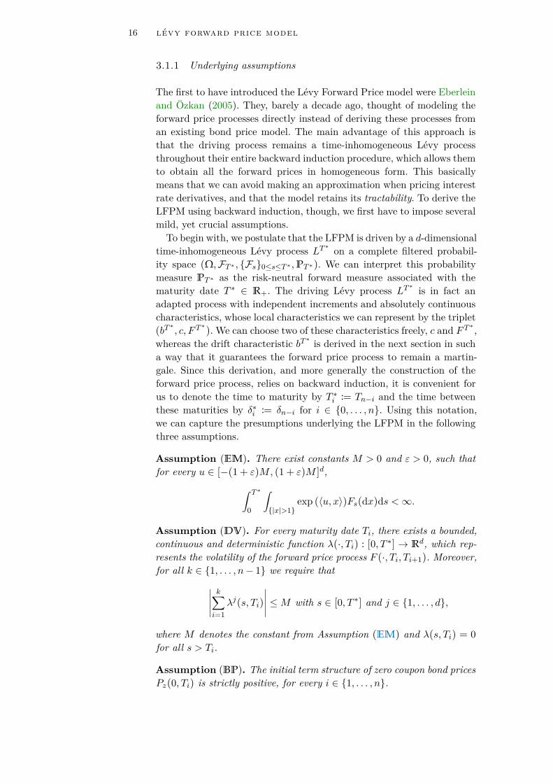
The first to have introduced the Lévy Forward Price model were Eberleinand Özkan (2005). They, barely a decade ago, thought of modeling theforward price processes directly instead of deriving these processes froman existing bond price model. The main advantage of this approach isthat the driving process remains a time-inhomogeneous Lévy processthroughout their entire backward induction procedure, which allows themto obtain all the forward prices in homogeneous form. This basicallymeans that we can avoid making an approximation when pricing interestrate derivatives, and that the model retains its tractability. To derive theLFPM using backward induction, though, we first have to impose severalmild, yet crucial assumptions.To begin with, we postulate that the LFPM is driven by a d-dimensional
time-inhomogeneous Lévy process LT ∗ on a complete filtered probabil-ity space (Ω,FT ∗ , Fs0≤s≤T ∗ , PT ∗). We can interpret this probabilitymeasure PT ∗ as the risk-neutral forward measure associated with thematurity date T ∗ ∈ R+. The driving Lévy process LT ∗ is in fact anadapted process with independent increments and absolutely continuouscharacteristics, whose local characteristics we can represent by the triplet(bT
∗ , c,F T ∗). We can choose two of these characteristics freely, c and F T ∗ ,
whereas the drift characteristic bT ∗ is derived in the next section in sucha way that it guarantees the forward price process to remain a martin-gale. Since this derivation, and more generally the construction of theforward price process, relies on backward induction, it is convenient forus to denote the time to maturity by T ∗i := Tn−i and the time betweenthese maturities by δ∗i := δn−i for i ∈ 0, . . . ,n. Using this notation,we can capture the presumptions underlying the LFPM in the followingthree assumptions.
Assumption (EM). There exist constants M > 0 and ε > 0, such thatfor every u ∈ [−(1 + ε)M , (1 + ε)M ]d,∫ T ∗
0
∫|x|>1
exp (〈u,x〉)Fs(dx)ds <∞.
Assumption (DV). For every maturity date Ti, there exists a bounded,continuous and deterministic function λ(·,Ti) : [0,T ∗] → Rd, which rep-resents the volatility of the forward price process F (·,Ti,Ti+1). Moreover,for all k ∈ 1, . . . ,n− 1 we require that∣∣∣∣∣
k∑i=1
λj(s,Ti)∣∣∣∣∣ ≤M with s ∈ [0,T ∗] and j ∈ 1, . . . , d,
where M denotes the constant from Assumption (EM) and λ(s,Ti) = 0for all s > Ti.
Assumption (BP). The initial term structure of zero coupon bond pricesPz(0,Ti) is strictly positive, for every i ∈ 1, . . . ,n.

3.1 model specification 17
These three rather basic assumptions are in fact all we need to imposein the LFPM. The first assumption essentially implies that the drivingprocess LT ∗ has finite exponential moments, which we typically requirea priori for the underlying process in an interest rate model to be amartingale. The importance of this assumption is that, in turn, it allowsus to price derivatives in a consistent, risk-neutral manner. The secondassumption furthermore merely restricts the volatility structure to beof bounded deterministic form, as extensively discussed in Section 2.3.1.Although the first two assumptions tend to be rather abstract and aresomewhat more demanding, the third assumption is a very mild initialcondition, where we only require the initial term structure of zero couponbond prices to be strictly positive. Together, these three assumptionsform the foundation of the LFPM.Now that we have explained and imposed the three most crucial as-
sumptions underlying the LFPM, we can fully devote our attention tothe construction of the forward price process by backward induction.
3.1.2 Construction of the forward price process
While the importance and the necessity of imposing Assumptions (EM),(DV) and (BP) has only been touched upon briefly in the previous sec-tion, its relevance will become clearer from the derivations in this section.To begin with, let us denote by 0 = T0 < T1 < · · · < Tn−1 < Tn = T ∗
a discrete tenor structure of times to maturity and set δk = Tk+1 − Tkequal to the time between these maturities. This, in turn, allows us tomore formally define the forward price process F (·,Tk,Tk+1) as
F (t,Tk,Tk+1) =Pz(t,Tk)Pz(t,Tk+1)
for every k ∈ 0, . . . ,n− 1.
In reality, we do not know these future prices of zero coupon bonds, andshould thus try to find a different expression for the forward price.One way we can construct the forward price process, is through back-
ward induction, where we first look at the forward price with the longesttime to maturity. For this forward price F (·,T ∗1 ,T ∗), we start by postu-lating that
F (t,T ∗1 ,T ∗) = F (0,T ∗1 ,T ∗) exp(∫ t
0λ(s,T ∗1 )dLT
∗s
), (2)
subject to the initial condition
F (0,T ∗1 ,T ∗) = Pz(0,T ∗1 )Pz(0,T ∗) .
Note that we can give an equivalent expression for Equation (2) in termsof the forward LIBOR rate L(·,T ∗1 ,T ∗) by
1 + δ∗1L(t,T ∗1 ,T ∗) = (1 + δ∗1L(0,T ∗1 ,T ∗)) exp(∫ t
0λ(s,T ∗1 )dLT
∗s
).

18 lévy forward price model
At this point, the main objective in our construction is to specify the driftcharacteristic bT ∗ in such a way that the forward price process F (·,T ∗1 ,T ∗)is a martingale with respect to its forward measure PT ∗ . To this end, wedefine bT ∗ such that∫ t
0
⟨λ(s,T ∗1 ), bT
∗s
⟩ds = −1
2
∫ t
0〈λ(s,T ∗1 ), csλ(s,T ∗1 )〉ds
−∫ t
0
∫Rd
(e〈λ(s,T
∗1 ),x〉 − 1− 〈λ(s,T ∗1 ),x〉
)νT
∗(ds, dx) , (3)
where we denote by νT ∗(ds, dx) := F T
∗s (dx) ds the compensator of the
random measure µL associated with the jumps of the Lévy process LT ∗ .Moreover, we can now apply Lemma 2.6 in Kallsen and Shiryaev (2002)to express the forward price in Equation (2) as the stochastic exponentialof a local martingale, yielding
F (t,T ∗1 ,T ∗) = F (0,T ∗1 ,T ∗)Et(H(·,T ∗1 ))
with
H(t,T ∗1 ) =∫ t
0
√csλ(s,T ∗1 ) dW T ∗
s
+∫ t
0
∫Rd
(e〈λ(s,T
∗1 ),x〉 − 1
)(µL − νT ∗)
(ds, dx) . (4)
Note that this local martingale H(·,T ∗1 ) is in fact a time-inhomogeneousLévy process as well. Eberlein et al. (2005) prove that, in this partic-ular case where the stochastic exponential of a process is both a localmartingale and a time-inhomogeneous Lévy process, it is not just a localmartingale but actually a martingale as well. As a consequence, we canconclude that the forward price process F (·,T ∗1 ,T ∗) and the correspond-ing forward LIBOR rate L(·,T ∗1 ,T ∗) are in fact martingales themselveswith respect to their forward measure PT ∗ .
This conclusion that the forward price process F (·,T ∗1 ,T ∗) is not onlya local martingale but even a martingale, has a crucial implication forthe remaining part of our derivation. This result actually allows us todefine the forward martingale measure associated with the maturity dateT ∗1 , by denoting
dPT ∗1
dPT ∗=F (T ∗1 ,T ∗1 ,T ∗)F (0,T ∗1 ,T ∗) = ET ∗
1(H(·,T ∗1 )).
Moreover, we can now apply Girsanov’s Theorem for semimartingales, seefor instance Theorem III.3.24 in Jacod and Shiryaev (2003), to identifythe two previsible processes β and Y from Equation (4) that describethis change of measure, by recognizing that
β(s) = λ(s,T ∗1 ) and Y (s,x) = exp (〈λ(s,T ∗1 ),x〉).
As a consequence, we have that

3.1 model specification 19
WT ∗
1t := W T ∗
t −∫ t
0
√csλ(s,T ∗1 ) ds,
νT∗1 (dt, dx) := exp (〈λ(t,T ∗1 ),x〉)F T
∗t (dx)dt
denote a standard Brownian motion under its forward measure PT ∗1and
the PT ∗1-compensator of µL, respectively. This yields the PT ∗
1-canonical
representation of the time-inhomogeneous Lévy process LT ∗ , given by
LT∗
t =∫ t
0bs ds+
∫ t
0
√cs dW T ∗
1s +
∫ t
0
∫Rdx(µL − νT ∗
1)(ds, dx), (5)
where we can calculate the deterministic drift coefficient b with Girsanov’sTheorem.
In turn, we can now construct the forward price process F (·,T ∗2 ,T ∗1 )through backward induction. Similarly to Equations (2) and (5), we canpostulate that
F (t,T ∗2 ,T ∗1 ) = F (0,T ∗2 ,T ∗1 ) exp(∫ t
0λ(s,T ∗2 )dL
T ∗1s
),
where
LT ∗
1t =
∫ t
0bT ∗
1s ds+
∫ t
0
√cs dW T ∗
1s +
∫ t
0
∫Rdx(µL − νT ∗
1)(ds, dx).
In this case, we can again specify the drift characteristic bT∗1 of the
driving Lévy process LT ∗1 in such a way that the forward price process
F (·,T ∗2 ,T ∗1 ) remains a martingale with respect to its forward measurePT ∗
1. This means that we, analogously to Equation (3), define bT ∗
1 suchthat ∫ t
0
⟨λ(s,T ∗2 ), b
T ∗1s
⟩ds = −1
2
∫ t
0〈λ(s,T ∗2 ), csλ(s,T ∗2 )〉 ds
−∫ t
0
∫Rd
(e〈λ(s,T
∗2 ),x〉 − 1− 〈λ(s,T ∗2 ),x〉
)νT
∗1 (ds, dx) .
In this way, the driving Lévy processes LT ∗1 and LT
∗ stay more or lessthe same, apart from a deterministic drift term, and remain in facttime-inhomogeneous processes under their respective forward measure.Likewise, we can again express the forward price process F (·,T ∗2 ,T ∗1 )as the stochastic exponential of both a local martingale and a time-inhomogeneous Lévy process H(·,T ∗2 ), yielding a martingale itself. Bythe same methodology, we can now actually define the forward martin-gale measure associated with the maturity date T ∗2 as
dPT ∗2
dPT ∗1
=F (T ∗2 ,T ∗2 ,T ∗1 )F (0,T ∗2 ,T ∗1 )
.
This recursive relationship between the forward martingale measures, inturn, allows us to construct the next forward price process F (·,T ∗3 ,T ∗2 )by backward induction as well.
20 lévy forward price model
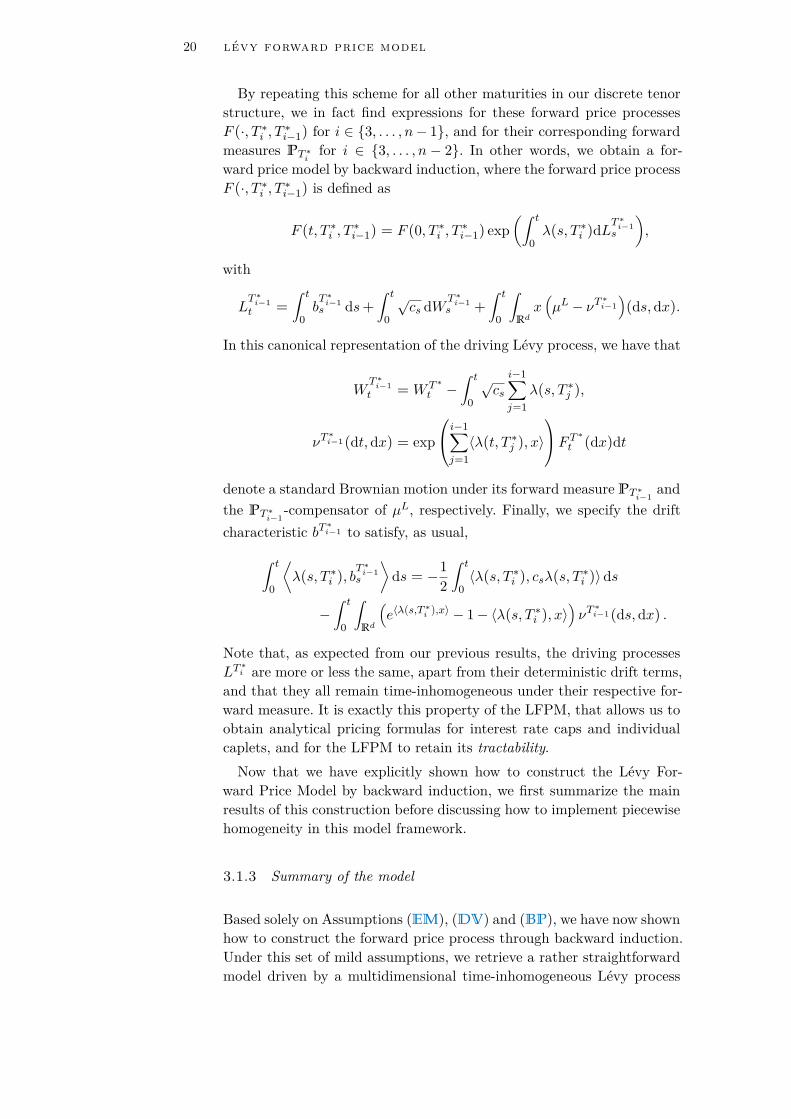
By repeating this scheme for all other maturities in our discrete tenorstructure, we in fact find expressions for these forward price processesF (·,T ∗i ,T ∗i−1) for i ∈ 3, . . . ,n− 1, and for their corresponding forwardmeasures PT ∗
ifor i ∈ 3, . . . ,n − 2. In other words, we obtain a for-
ward price model by backward induction, where the forward price processF (·,T ∗i ,T ∗i−1) is defined as
F (t,T ∗i ,T ∗i−1) = F (0,T ∗i ,T ∗i−1) exp(∫ t
0λ(s,T ∗i )dL
T ∗i−1s
),
with
LT ∗i−1t =
∫ t
0bT ∗i−1s ds+
∫ t
0
√cs dW T ∗
i−1s +
∫ t
0
∫Rdx(µL − νT
∗i−1)(ds, dx).
In this canonical representation of the driving Lévy process, we have that
WT ∗i−1
t = W T ∗t −
∫ t
0
√cs
i−1∑j=1
λ(s,T ∗j ),
νT∗i−1(dt, dx) = exp
i−1∑j=1〈λ(t,T ∗j ),x〉
F T ∗t (dx)dt
denote a standard Brownian motion under its forward measure PT ∗i−1
andthe PT ∗
i−1-compensator of µL, respectively. Finally, we specify the drift
characteristic bT∗i−1 to satisfy, as usual,
∫ t
0
⟨λ(s,T ∗i ), b
T ∗i−1s
⟩ds = −1
2
∫ t
0〈λ(s,T ∗i ), csλ(s,T ∗i )〉ds
−∫ t
0
∫Rd
(e〈λ(s,T
∗i ),x〉 − 1− 〈λ(s,T ∗i ),x〉
)νT
∗i−1(ds, dx) .
Note that, as expected from our previous results, the driving processesLT
∗i are more or less the same, apart from their deterministic drift terms,
and that they all remain time-inhomogeneous under their respective for-ward measure. It is exactly this property of the LFPM, that allows us toobtain analytical pricing formulas for interest rate caps and individualcaplets, and for the LFPM to retain its tractability.Now that we have explicitly shown how to construct the Lévy For-
ward Price Model by backward induction, we first summarize the mainresults of this construction before discussing how to implement piecewisehomogeneity in this model framework.
3.1.3 Summary of the model
Based solely on Assumptions (EM), (DV) and (BP), we have now shownhow to construct the forward price process through backward induction.Under this set of mild assumptions, we retrieve a rather straightforwardmodel driven by a multidimensional time-inhomogeneous Lévy process

3.1 model specification 21
that in fact remains time-inhomogeneous under each respective forwardmeasure. Before we move on to investigate how we can best parameterizeour piecewise homogeneity restriction in the LFPM, we summarize themain characteristics of the LFPM and some of the most fundamentalresults from our construction of the forward price process.Through backward induction, we have been able to obtain all forward
prices in homogeneous form, which allows us to avoid making an ap-proximation in the pricing of derivatives. This form of the forward priceprocesses in the LFPM is characterized by
F (t,T ∗i ,T ∗i−1) = F (0,T ∗i ,T ∗i−1) exp(∫ t
0λ(s,T ∗i )dL
T ∗i−1s
),
subject to the initial condition
F (0,T ∗i ,T ∗i−1) =Pz(0,T ∗i )Pz(0,T ∗i−1)
and where we define the d-dimensional time-inhomogeneous Lévy processLT
∗i−1 by its PT ∗
i−1-canonical representation as
LT ∗i−1t =
∫ t
0bT ∗i−1s ds+
∫ t
0
√cs dW T ∗
i−1s +
∫ t
0
∫Rdx(µL − νT
∗i−1)(ds, dx).
Moreover, we have that
WT ∗i−1
t = W T ∗t −
∫ t
0
√cs
i−1∑j=1
λ(s,T ∗j ) ds,
νT∗i−1(dt, dx) = exp
i−1∑j=1〈λ(t,T ∗j ),x〉
F T ∗t (dx)dt
denote a standard Brownian motion under its risk-neutral forward mea-sure PT ∗
i−1and the PT ∗
i−1-compensator of µL, respectively. Finally, the
drift characteristic bT∗i−1 is specified to satisfy
∫ t
0
⟨λ(s,T ∗i ), b
T ∗i−1s
⟩ds = −1
2
∫ t
0〈λ(s,T ∗i ), csλ(s,T ∗i )〉 ds
−∫ t
0
∫Rd
(e〈λ(s,T
∗i ),x〉 − 1− 〈λ(s,T ∗i ),x〉
)νT
∗i−1(ds, dx) ,
which ensures that the driving Lévy process remains a martingale underits respective forward measure. As a result, we find that the drivingprocesses LT ∗
i are more or less the same, apart from their deterministicdrift terms, and that they all remain time-inhomogeneous under theirrespective forward measure. As a consequence, the LFPM retains itstractability and offers us the possibility to price interest rate caps andindividual caplets through closed-form, analytical formulas.With this insight into the inner workings of the LFPM and the time-
inhomogeneity property of the driving process, it is possible to derive an

22 lévy forward price model
explicit pricing formula for interest rate caps and individual caplets. How-ever, before we can do so, we first have to address the parameterizationof our piecewise homogeneity restriction.
3.2 piecewise homogeneity
Although the construction of the forward price process in the previous sec-tions resides on only three quite mild assumptions, the exact formulas arenot left unaltered if we impose piecewise homogeneity. As argued in Sec-tion 2.3.2, we impose piecewise homogeneity in the driving Lévy processto resolve the curse of dimensionality caused by the time-inhomogeneityproperty of the LFPM, and to ensure that the model leads to curve vari-ation. Moreover, by allowing for both deterministic and random break-points in the parameters of the three time-homogeneous Lévy processes,we investigate whether this additional flexibility yields any improvementsin terms of the model performance criteria in Section 2.4. Even thoughimposing this restriction is far from uncommon in the literature, see forinstance Eberlein and Kluge (2007) and Eberlein et al. (2016), the exactparameterization and implications of piecewise homogeneity have stillbeen left unspecified. Moreover, these supplemental features do come ata cost, since they actually affect some of the defining characteristics of theLFPM. To assess this effect, we review the fundamental results derivedin the previous sections under this piecewise homogeneity restriction.The time-inhomogeneity property of the driving Lévy process essen-
tially implies that its local characteristics vary through time. From amathematical perspective, this basically means that the increments of theLévy process are not stationary through time, but depend on the momentof observation. If we replace the driving time-inhomogeneous Lévy pro-cess with three separate time-homogeneous Lévy processes, each designedfor a different set of times to maturity, we actually obtain stationary incre-ments of each separate Lévy process. This, in turn, implies that the localcharacteristics of the driving processes no longer vary through time, butare in fact, piecewise, time-invariant. Each separate time-homogeneousLévy process is thus associated with a different set of times to maturity,where in the deterministic case the first one corresponds to maturitiesup to roughly one year, the second one to maturities between one andfive years, and the third one to maturities of at least five years. Together,these three processes actually enable us to realize curve variation in theLFPM, since we can directly relate the three processes to variation inparallel shifts, curvature and steepness.Therefore, the only severe consequence of this rather mild form of time-
inhomogeneity seems to be that the local characteristics of the drivingprocesses are now time-invariant, instead of varying through time. Morespecifically, in our formulas, we only need to change the time-varyingtriplet (b
T ∗i−1t , ct,F
T ∗i−1
t ) into the three piecewise time-invariant triplets(bT ∗i−1S , cS ,F T
∗i−1
S ), (bT∗i−1M , cM ,F T
∗i−1
M ) and (bT ∗i−1L , cL,F T
∗i−1
L ) for short-termmaturities t ∈ [0,ϕ], medium-term maturities t ∈ (ϕ,ψ] and long-term
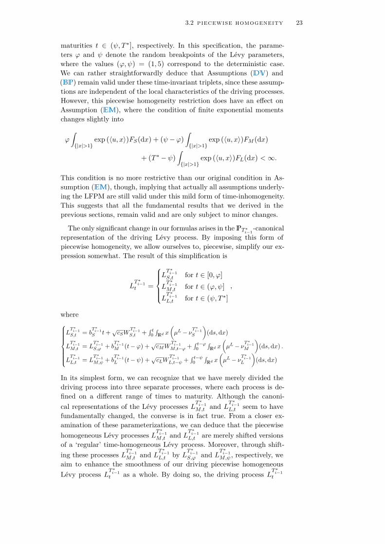
3.2 piecewise homogeneity 23
maturities t ∈ (ψ,T ∗], respectively. In this specification, the parame-ters ϕ and ψ denote the random breakpoints of the Lévy parameters,where the values (ϕ,ψ) = (1, 5) correspond to the deterministic case.We can rather straightforwardly deduce that Assumptions (DV) and(BP) remain valid under these time-invariant triplets, since these assump-tions are independent of the local characteristics of the driving processes.However, this piecewise homogeneity restriction does have an effect onAssumption (EM), where the condition of finite exponential momentschanges slightly into
ϕ
∫|x|>1
exp (〈u,x〉)FS(dx) + (ψ−ϕ)∫|x|>1
exp (〈u,x〉)FM (dx)
+ (T ∗ − ψ)∫|x|>1
exp (〈u,x〉)FL(dx) < ∞.
This condition is no more restrictive than our original condition in As-sumption (EM), though, implying that actually all assumptions underly-ing the LFPM are still valid under this mild form of time-inhomogeneity.This suggests that all the fundamental results that we derived in theprevious sections, remain valid and are only subject to minor changes.
The only significant change in our formulas arises in the PT ∗i−1
-canonicalrepresentation of the driving Lévy process. By imposing this form ofpiecewise homogeneity, we allow ourselves to, piecewise, simplify our ex-pression somewhat. The result of this simplification is
LT ∗i−1t =
LT ∗i−1S,t for t ∈ [0,ϕ]
LT ∗i−1M ,t for t ∈ (ϕ,ψ]
LT ∗i−1L,t for t ∈ (ψ,T ∗]
,
where
LT ∗i−1S,t = b
T ∗i−1S t+
√cSW
T ∗i−1
S,t +∫ t
0∫
Rd x
(µL − νT
∗i−1
S
)(ds, dx)
LT ∗i−1M ,t = L
T ∗i−1S,ϕ + b
T ∗i−1M (t−ϕ) +√cMW
T ∗i−1
M ,t−ϕ +∫ t−ϕ
0∫
Rd x
(µL − νT
∗i−1
M
)(ds, dx) .
LT ∗i−1L,t = L
T ∗i−1M ,ψ + b
T ∗i−1L (t−ψ) +√cLW
T ∗i−1
L,t−ψ +∫ t−ψ
0∫
Rd x
(µL − νT
∗i−1
L
)(ds, dx)
In its simplest form, we can recognize that we have merely divided thedriving process into three separate processes, where each process is de-fined on a different range of times to maturity. Although the canoni-cal representations of the Lévy processes LT
∗i−1M ,t and LT
∗i−1L,t seem to have
fundamentally changed, the converse is in fact true. From a closer ex-amination of these parameterizations, we can deduce that the piecewisehomogeneous Lévy processes LT
∗i−1M ,t and LT
∗i−1L,t are merely shifted versions
of a ‘regular’ time-homogeneous Lévy process. Moreover, through shift-ing these processes LT
∗i−1M ,t and LT
∗i−1L,t by LT
∗i−1S,ϕ and LT
∗i−1M ,ψ , respectively, we
aim to enhance the smoothness of our driving piecewise homogeneousLévy process LT
∗i−1t as a whole. By doing so, the driving process LT
∗i−1t

24 lévy forward price model
does not exhibit a sudden jump after one of the breakpoints ϕ and ψ
due to a change in the Lévy parameters, but tends to gradually follow adifferent path only after these breakpoints. As a consequence, the driv-ing process remains rather smooth, while simultaneously enabling us torealize curve variation. More importantly, though, since these piecewisehomogeneous Lévy processes are simply shifted time-homogeneous Lévyprocesses under our parameterization, we can still follow our approachin the previous sections and construct the forward price process throughbackward induction. In other words, despite some minor changes, ourconstruction of the forward price process remains unaltered, and, as aresult, all the fundamental characteristics of the LFPM stay more or lessthe same.It has thus become apparent that imposing piecewise homogeneity has
only minor consequences for the construction of the forward price process,while it offers us significant benefits for calibrating the LFPM to actualmarket data. However, before we can estimate these model extensionswith actual market prices of caps, we first need to know how to consis-tently price these interest rate derivatives in the LFPM framework.
3.3 pricing interest rate caps
From the construction of the forward price process, it has become appar-ent that we can price caps and individual caplets in the LFPM throughclosed-form, analytical formulas. In Section 3.1.2, we have seen that thetime-inhomogeneity property of the driving Lévy process is preserved bybackward induction, which allows us to consistently price interest ratederivatives and to avoid making an approximation in doing so. By im-posing piecewise homogeneity in this model framework, we have beenable to resolve the curse of dimensionality associated with the drivingtime-inhomogeneous Lévy process and to ensure that the LFPM satis-fies curve variation. More importantly, though, the construction of theforward price process remains valid under this piecewise homogeneityrestriction, meaning that we can still price interest rate caps and indi-vidual caplets through closed-form, analytical formulas. To this end, wefirst briefly discuss the relation between caps and individual caplets, afterwhich we present an explicit Fourier-based formula to value this type ofinterest rate derivative.A cap is one of the most popular and liquid interest rate derivatives in
the derivatives market nowadays, consisting of a sequence of call optionson consecutive LIBOR rates. Each of these separate call options is calleda caplet, implying that a cap consists of a series of individual caplets.A caplet is characterized by its time to maturity T ∗i , strike rate K andnotional amount N . With these characteristics, we can represent thepayoff of a caplet at its payment date T ∗i−1 in terms of the forward LIBORrate L(·,T ∗i ,T ∗i−1) by
Nδ∗j (L(T∗i ,T ∗i ,T ∗i−1)−K)+ ,
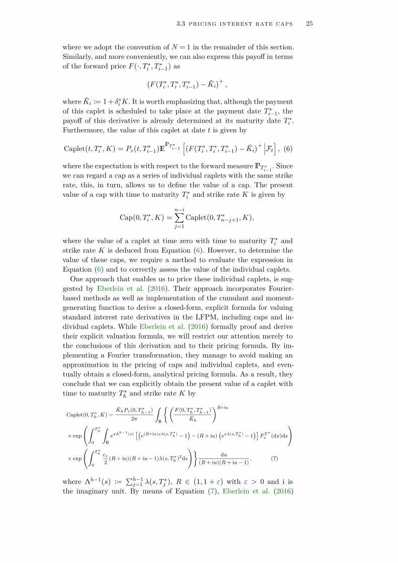
3.3 pricing interest rate caps 25
where we adopt the convention of N = 1 in the remainder of this section.Similarly, and more conveniently, we can also express this payoff in termsof the forward price F (·,T ∗i ,T ∗i−1) as(
F (T ∗i ,T ∗i ,T ∗i−1)− Ki)+ ,
where Ki := 1+ δ∗iK. It is worth emphasizing that, although the paymentof this caplet is scheduled to take place at the payment date T ∗i−1, thepayoff of this derivative is already determined at its maturity date T ∗i .Furthermore, the value of this caplet at date t is given by
Caplet(t,T ∗i ,K) = Pz(t,T ∗i−1)EPT∗
i−1[(F (T ∗i ,T ∗i ,T ∗i−1)− Ki
)+ ∣∣∣Ft] , (6)
where the expectation is with respect to the forward measure PT ∗i−1
. Sincewe can regard a cap as a series of individual caplets with the same strikerate, this, in turn, allows us to define the value of a cap. The presentvalue of a cap with time to maturity T ∗i and strike rate K is given by
Cap(0,T ∗i ,K) =n−i∑j=1
Caplet(0,T ∗n−j+1,K),
where the value of a caplet at time zero with time to maturity T ∗i andstrike rate K is deduced from Equation (6). However, to determine thevalue of these caps, we require a method to evaluate the expression inEquation (6) and to correctly assess the value of the individual caplets.
One approach that enables us to price these individual caplets, is sug-gested by Eberlein et al. (2016). Their approach incorporates Fourier-based methods as well as implementation of the cumulant and moment-generating function to derive a closed-form, explicit formula for valuingstandard interest rate derivatives in the LFPM, including caps and in-dividual caplets. While Eberlein et al. (2016) formally proof and derivetheir explicit valuation formula, we will restrict our attention merely tothe conclusions of this derivation and to their pricing formula. By im-plementing a Fourier transformation, they manage to avoid making anapproximation in the pricing of caps and individual caplets, and even-tually obtain a closed-form, analytical pricing formula. As a result, theyconclude that we can explicitly obtain the present value of a caplet withtime to maturity T ∗h and strike rate K by
Caplet(0,T ∗h ,K) =
KhPz(0,T ∗h−1)
2π
∫R
(F (0,T ∗
h ,T ∗h−1)
Kh
)R+iu
× exp
(∫ T∗h
0
∫R
exΛh−1(s)[(e(R+iu)xλ(s,T∗
h) − 1
)− (R+ iu)
(exλ(s,T∗
h) − 1
)]FT
∗s (dx)ds
)
× exp
(∫ T∗h
0
cs
2(R+ iu)(R+ iu− 1)λ(s,T ∗
h )2ds
)du
(R+ iu)(R+ iu− 1), (7)
where Λh−1(s) :=∑h−1j=1 λ(s,T ∗j ), R ∈ (1, 1 + ε) with ε > 0 and i is
the imaginary unit. By means of Equation (7), Eberlein et al. (2016)

26 lévy forward price model
thus provide us with a closed-form solution to the pricing problem ofcaps and individual caplets. Through implementation of their analyticalpricing formula, we can now calibrate our extensions of the LFPM toactual market data on interest rate caplets and compare the empiricalperformance of these model extensions.To conclude, we have presented a formal construction of the forward
price process in the LFPM in this chapter, and have elaborated on someof the most essential characteristics of this model framework. Next, wehave discussed how to explicitly parameterize our piecewise homogeneityrestriction, and how this restriction affects the construction of the forwardprice process in the LFPM. Finally, we have argued how to consistentlyprice interest rate caps and individual caplets, by means of a closed-form,analytical expression.

4DATA AND OPTIMIZAT ION ROUTINES
Having shown how to analytically price interest rate caplets in the LFPMenables us to calibrate our model extensions to actual market data. How-ever, to calibrate the LFPM, we do not only require the market prices ofinterest rate caplets, but the term structure of zero coupon bond pricesas well. It is therefore of crucial importance to understand how we cantransform the implied Black volatilities of caps quoted by the market toobtain the corresponding market price of each individual caplet, and howto acquire the term structure of zero coupon bond prices. In addition,we require an optimization scheme for the minimization of our nonlinearcriterion function with the market data, once we have been able to moldthese data into the correct form.
This chapter primarily focuses on the transformation of these impliedBlack volatilities and obtaining the term structure of zero coupon bondprices, as well as on how to optimize our nonlinear criterion function.We first explain how to retrieve the relevant market prices in the nextsection, along with a formal presentation of the market data employedin this thesis.
4.1 financial market data
In the previous chapter we have seen how to price caplets in the LFPM bymeans of a closed-form, analytical expression. This pricing formula high-lights the fact that we require market information on the term structureof zero coupon bond prices as well as on the prices of individual caplets.However, both of these financial products are not directly quoted by themarket, but need to be recovered indirectly from other sources of mar-ket information. We therefore adopt the bootstrap method mentionedin Veronesi (2010) to retrieve the term structure of zero coupon bondprices, whereas we follow the stripping procedure outlined in Brigo andMercurio (2007) to obtain the market price of each individual caplet.
27
28 data and optimization routines
While the bootstrap method only requires market swap rates to recoverthe term structure of zero coupon bond prices, the stripping procedureresides on both the market prices of caps and the term structure of zerocoupon bond prices. We therefore first implement the bootstrap methodsuggested by Veronesi (2010) in the following section, before applying thestripping procedure described by Brigo and Mercurio (2007).
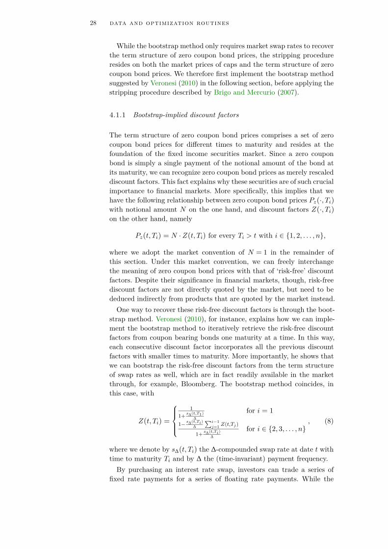
4.1.1 Bootstrap-implied discount factors
The term structure of zero coupon bond prices comprises a set of zerocoupon bond prices for different times to maturity and resides at thefoundation of the fixed income securities market. Since a zero couponbond is simply a single payment of the notional amount of the bond atits maturity, we can recognize zero coupon bond prices as merely rescaleddiscount factors. This fact explains why these securities are of such crucialimportance to financial markets. More specifically, this implies that wehave the following relationship between zero coupon bond prices Pz(·,Ti)with notional amount N on the one hand, and discount factors Z(·,Ti)on the other hand, namely
Pz(t,Ti) = N ·Z(t,Ti) for every Ti > t with i ∈ 1, 2, . . . ,n,
where we adopt the market convention of N = 1 in the remainder ofthis section. Under this market convention, we can freely interchangethe meaning of zero coupon bond prices with that of ‘risk-free’ discountfactors. Despite their significance in financial markets, though, risk-freediscount factors are not directly quoted by the market, but need to bededuced indirectly from products that are quoted by the market instead.One way to recover these risk-free discount factors is through the boot-
strap method. Veronesi (2010), for instance, explains how we can imple-ment the bootstrap method to iteratively retrieve the risk-free discountfactors from coupon bearing bonds one maturity at a time. In this way,each consecutive discount factor incorporates all the previous discountfactors with smaller times to maturity. More importantly, he shows thatwe can bootstrap the risk-free discount factors from the term structureof swap rates as well, which are in fact readily available in the marketthrough, for example, Bloomberg. The bootstrap method coincides, inthis case, with
Z(t,Ti) =
1
1+ s∆(t,T1)∆
for i = 1
1− s∆(t,Ti)∆
∑i−1j=1 Z(t,Tj)
1+ s∆(t,Ti)∆
for i ∈ 2, 3, . . . ,n, (8)
where we denote by s∆(t,Ti) the ∆-compounded swap rate at date t withtime to maturity Ti and by ∆ the (time-invariant) payment frequency.By purchasing an interest rate swap, investors can trade a series of
fixed rate payments for a series of floating rate payments. While the
4.1 financial market data 29
fixed rate payment is determined by the swap rate of the interest rateswap, the floating rate payment is in fact linked to a specific index, suchas the 6-month LIBOR rate, for instance. However, from ECB’s annualsupervisory stress test in Figure 1 we can deduce that the concerns fornegative interest rates are particularly prevailing in the Eurozone. Thisimplies that, from a risk management perspective, it is more relevantto consider the 6-month EURIBOR rate as the underlying index of theswap, instead of the 6-month LIBOR rate.
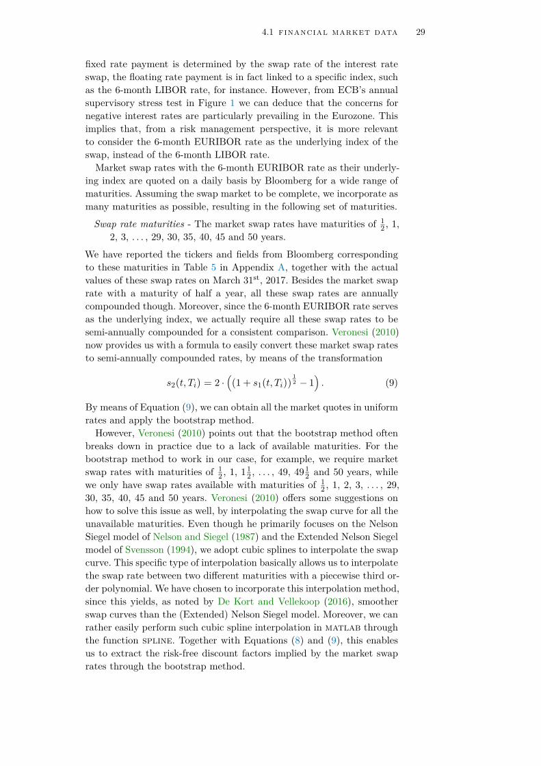
Market swap rates with the 6-month EURIBOR rate as their underly-ing index are quoted on a daily basis by Bloomberg for a wide range ofmaturities. Assuming the swap market to be complete, we incorporate asmany maturities as possible, resulting in the following set of maturities.
Swap rate maturities - The market swap rates have maturities of 12 , 1,
2, 3, . . . , 29, 30, 35, 40, 45 and 50 years.
We have reported the tickers and fields from Bloomberg correspondingto these maturities in Table 5 in Appendix A, together with the actualvalues of these swap rates on March 31st, 2017. Besides the market swaprate with a maturity of half a year, all these swap rates are annuallycompounded though. Moreover, since the 6-month EURIBOR rate servesas the underlying index, we actually require all these swap rates to besemi-annually compounded for a consistent comparison. Veronesi (2010)now provides us with a formula to easily convert these market swap ratesto semi-annually compounded rates, by means of the transformation
s2(t,Ti) = 2 ·((1 + s1(t,Ti))
12 − 1
). (9)
By means of Equation (9), we can obtain all the market quotes in uniformrates and apply the bootstrap method.However, Veronesi (2010) points out that the bootstrap method often
breaks down in practice due to a lack of available maturities. For thebootstrap method to work in our case, for example, we require marketswap rates with maturities of 1
2 , 1, 112 , . . . , 49, 491
2 and 50 years, whilewe only have swap rates available with maturities of 1
2 , 1, 2, 3, . . . , 29,30, 35, 40, 45 and 50 years. Veronesi (2010) offers some suggestions onhow to solve this issue as well, by interpolating the swap curve for all theunavailable maturities. Even though he primarily focuses on the NelsonSiegel model of Nelson and Siegel (1987) and the Extended Nelson Siegelmodel of Svensson (1994), we adopt cubic splines to interpolate the swapcurve. This specific type of interpolation basically allows us to interpolatethe swap rate between two different maturities with a piecewise third or-der polynomial. We have chosen to incorporate this interpolation method,since this yields, as noted by De Kort and Vellekoop (2016), smootherswap curves than the (Extended) Nelson Siegel model. Moreover, we canrather easily perform such cubic spline interpolation in matlab throughthe function spline. Together with Equations (8) and (9), this enablesus to extract the risk-free discount factors implied by the market swaprates through the bootstrap method.

30 data and optimization routines
Figure 2. Swap curves on March 30th, 2012 up until April 28th, 2017.Swap curves on a semi-annual basis for maturities ranging from half a year to50 years. The swap curves consist of the market rates on March 30th, 2012 upuntil April 28th, 2017 and are interpolated for intermediate maturities throughcubic spline interpolation.
Figure 3. Implied discount factors on March 30th, 2012 up until April28th, 2017. Discount factors on a semi-annual basis for maturities rangingfrom half a year to 50 years. These discount factors are extracted from theswap curves on March 30th, 2012 up until April 28th, 2017 in Figure 2 throughimplementation of the bootstrap method in Equation (8).
We have applied this bootstrap methodology to daily quotes of themarket swap rates from Bloomberg for several years. More specifically,we have included data of the swap rates on March 30th, 2012 up untilApril 28th, 2017 in this method. While we explicitly assess the goodness-

4.1 financial market data 31
of-fit of our model extensions of the LFPM on March 31st, 2017 in thenext chapter, we determine the parameter stability with market data onMarch 30th, 2012 up until March 31st, 2017. The most recent month in ourdataset, comprising March 31st, 2017 up until April 28th, 2012, is left toevaluate the out-of-sample pricing performance of our model extensions.To this end, we show the results from the bootstrap methodology on ourentire dataset in Figures 2 and 3, whereas we explicitly depict the swapcurve and its implied discount factors on March 30th, 2012, September30th, 2014 and on March 31st, 2017 in Figures A.1 and A.2 in Appendix A,respectively.The results from this bootstrap method highlight the facts that neg-
ative rates can occur nowadays and that market rates generally do notremain constant through time particularly well. However, we should notethat on certain days in our dataset, some market swap rates were notquoted by Bloomberg. This issue only arises eight times in our entiredataset, though, and from Figure A.3, we can see that these marketswap rates barely change from day to day. We have therefore simply in-terpolated linearly the swap rates quoted on the two closest trading dayswith the same maturity to retrieve an estimate of these unavailable val-ues. In addition, there appear to be three outliers in our dataset that areextremely out of line with the other market swap rates. The outliers inquestion are the swap rates with a maturity of 18 years, 21 years and 23years on April 14th, 2017, and give rise to a change in the swap rate of al-most twenty times the standard error above the average daily change. Toreplace these significant deviations and to obtain a smoother swap ratecurve, we have rather straightforwardly interpolated linearly the swaprates with the two closest maturities on the same trading day.Based on these bootstrapped discount factors, we are now in fact able
to transform the implied Black volatilities of caps to their correspond-ing market prices, and to, ultimately, retrieve the market price of eachindividual caplet. We focus on the methodology underlying this trans-formation in the following section, as well as how to obtain the impliedBlack volatilities of caps from the market.
4.1.2 Stripping caplet quotes from cap quotes
While we only required the market swap rates to bootstrap the implieddiscount factors, we need both the market prices of interest rate capsand these implied discount factors to strip the price of each individualcaplet. Moreover, even though the prices of interest rate caps are quotedindirectly by the market in terms of their implied Black volatilities, theprices of separate caplets are not specified by the market at all. However,as argued in Section 3.3, we can represent a cap as a series of individualcaplets with the same strike rate. From the market prices of caps andtheir implied Black volatilities, we can therefore iteratively deduce themarket prices of these caplets through the stripping procedure outlinedin Brigo and Mercurio (2007).

32 data and optimization routines
This procedure first requires us to convert the implied Black volatilitiesof caps to their corresponding market prices. To begin with, an impliedBlack volatility of a cap is that specific level of volatility that recoversthe market price of that particular cap by inserting its implied volatilityinto Black’s formula for an interest rate cap. We can represent Black’sformula for the present value of an interest rate cap with time to maturityT ∗i , strike rate K and implied volatility σ, formally by
CapBlack(0,T ∗i ,K,σ) =n−i∑j=1
Z(0,T ∗n−j)
×(F (0,T ∗n−j+1,T ∗n−j)Φ(d1(σ))− KΦ(d2(σ))
), (10)
where we denote by Φ(·) the standard Gaussian cumulative distributionfunction and where
d1(σ) =log
(F (0,T ∗
n−j+1,T ∗n−j)
K
)+ 1
2σ2T ∗n−j+1
σ√T ∗n−j+1
,
d2(σ) = d1 − σ√T ∗n−j+1.
From Equation (10) it now also becomes clear why we were first requiredto bootstrap the implied discount factors, since they enter into the ex-pression through the initial forward prices F (0,T ∗i ,T ∗i−1) and throughthe discount factors Z(0,T ∗i−1). Moreover, by inserting the implied Blackvolatility of a certain cap into Equation (10), we can rather straightfor-wardly obtain the market price of that particular cap.
These implied volatilities are quoted on a daily basis by Bloomberg fora wide range of both maturities and strike rates. While only the caps witha maturity of 1 year and 2 years are linked to the 3-month EURIBOR rate,all other caps have the 6-month rate as their underlying index. Moreover,since we only have implied discount factors on a semi-annual basis, weimpose the simplification that the caps with a maturity of 1 year and 2years are linked to the 6-month EURIBOR rate as well. Similarly to theswap market, we now assume the cap market to be complete and includeas many maturities and strike rates as possible, resulting in the followingsets of maturities and strike rates.
Interest rate cap maturities - The interest rate caps have maturities of1, 2, . . . , 9, 10, 12, 15 and 20 years.
Interest rate cap strike rates - The interest rate caps have strike ratesof 1.00%, 1.75%, 2.00%, 2.25%, 2.50%, 3.00%, 3.50%, 4.00%, 5.00%,6.00%, 7.00%, 8.00%. 9.00% and 10.00%, apart from at-the-money(ATM) strike rates.
We have reported the tickers and fields from Bloomberg correspondingto these maturities and strike rates in Table 6 in Appendix A, togetherwith the actual values of these implied Black volatilities on March 31st,
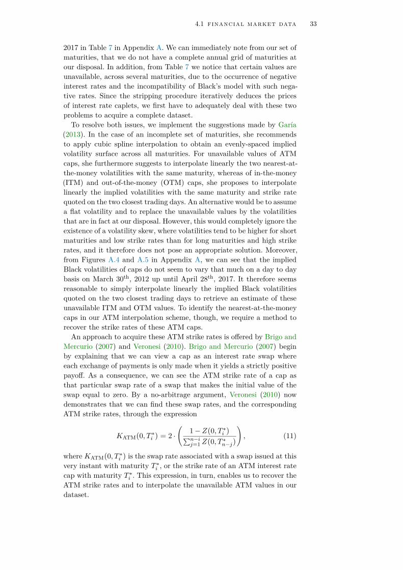
4.1 financial market data 33
2017 in Table 7 in Appendix A. We can immediately note from our set ofmaturities, that we do not have a complete annual grid of maturities atour disposal. In addition, from Table 7 we notice that certain values areunavailable, across several maturities, due to the occurrence of negativeinterest rates and the incompatibility of Black’s model with such nega-tive rates. Since the stripping procedure iteratively deduces the pricesof interest rate caplets, we first have to adequately deal with these twoproblems to acquire a complete dataset.To resolve both issues, we implement the suggestions made by Garía
(2013). In the case of an incomplete set of maturities, she recommendsto apply cubic spline interpolation to obtain an evenly-spaced impliedvolatility surface across all maturities. For unavailable values of ATMcaps, she furthermore suggests to interpolate linearly the two nearest-at-the-money volatilities with the same maturity, whereas of in-the-money(ITM) and out-of-the-money (OTM) caps, she proposes to interpolatelinearly the implied volatilities with the same maturity and strike ratequoted on the two closest trading days. An alternative would be to assumea flat volatility and to replace the unavailable values by the volatilitiesthat are in fact at our disposal. However, this would completely ignore theexistence of a volatility skew, where volatilities tend to be higher for shortmaturities and low strike rates than for long maturities and high strikerates, and it therefore does not pose an appropriate solution. Moreover,from Figures A.4 and A.5 in Appendix A, we can see that the impliedBlack volatilities of caps do not seem to vary that much on a day to daybasis on March 30th, 2012 up until April 28th, 2017. It therefore seemsreasonable to simply interpolate linearly the implied Black volatilitiesquoted on the two closest trading days to retrieve an estimate of theseunavailable ITM and OTM values. To identify the nearest-at-the-moneycaps in our ATM interpolation scheme, though, we require a method torecover the strike rates of these ATM caps.An approach to acquire these ATM strike rates is offered by Brigo and
Mercurio (2007) and Veronesi (2010). Brigo and Mercurio (2007) beginby explaining that we can view a cap as an interest rate swap whereeach exchange of payments is only made when it yields a strictly positivepayoff. As a consequence, we can see the ATM strike rate of a cap asthat particular swap rate of a swap that makes the initial value of theswap equal to zero. By a no-arbitrage argument, Veronesi (2010) nowdemonstrates that we can find these swap rates, and the correspondingATM strike rates, through the expression
KATM(0,T ∗i ) = 2 ·(
1−Z(0,T ∗i )∑n−ij=1 Z(0,T ∗n−j)
), (11)
where KATM(0,T ∗i ) is the swap rate associated with a swap issued at thisvery instant with maturity T ∗i , or the strike rate of an ATM interest ratecap with maturity T ∗i . This expression, in turn, enables us to recover theATM strike rates and to interpolate the unavailable ATM values in ourdataset.
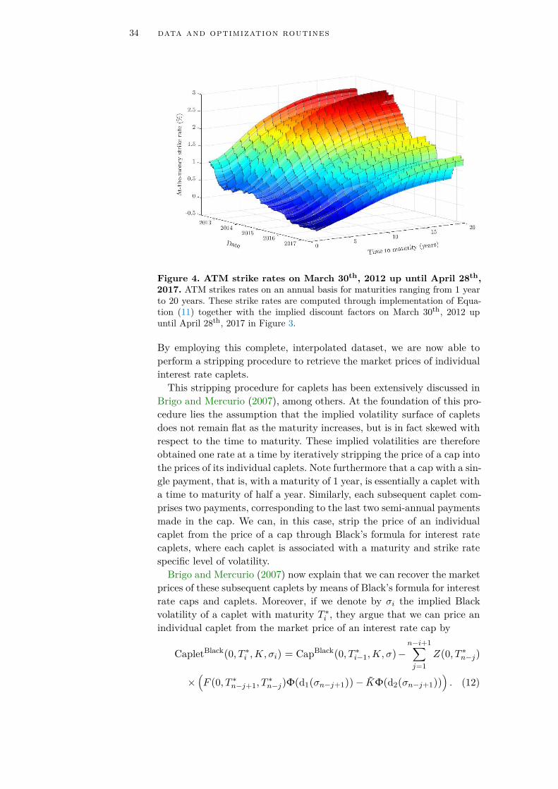
34 data and optimization routines
Figure 4. ATM strike rates on March 30th, 2012 up until April 28th,2017. ATM strikes rates on an annual basis for maturities ranging from 1 yearto 20 years. These strike rates are computed through implementation of Equa-tion (11) together with the implied discount factors on March 30th, 2012 upuntil April 28th, 2017 in Figure 3.
By employing this complete, interpolated dataset, we are now able toperform a stripping procedure to retrieve the market prices of individualinterest rate caplets.This stripping procedure for caplets has been extensively discussed in
Brigo and Mercurio (2007), among others. At the foundation of this pro-cedure lies the assumption that the implied volatility surface of capletsdoes not remain flat as the maturity increases, but is in fact skewed withrespect to the time to maturity. These implied volatilities are thereforeobtained one rate at a time by iteratively stripping the price of a cap intothe prices of its individual caplets. Note furthermore that a cap with a sin-gle payment, that is, with a maturity of 1 year, is essentially a caplet witha time to maturity of half a year. Similarly, each subsequent caplet com-prises two payments, corresponding to the last two semi-annual paymentsmade in the cap. We can, in this case, strip the price of an individualcaplet from the price of a cap through Black’s formula for interest ratecaplets, where each caplet is associated with a maturity and strike ratespecific level of volatility.Brigo and Mercurio (2007) now explain that we can recover the market
prices of these subsequent caplets by means of Black’s formula for interestrate caps and caplets. Moreover, if we denote by σi the implied Blackvolatility of a caplet with maturity T ∗i , they argue that we can price anindividual caplet from the market price of an interest rate cap by
CapletBlack(0,T ∗i ,K,σi) = CapBlack(0,T ∗i−1,K,σ)−n−i+1∑j=1
Z(0,T ∗n−j)
×(F (0,T ∗n−j+1,T ∗n−j)Φ(d1(σn−j+1))− KΦ(d2(σn−j+1))
). (12)
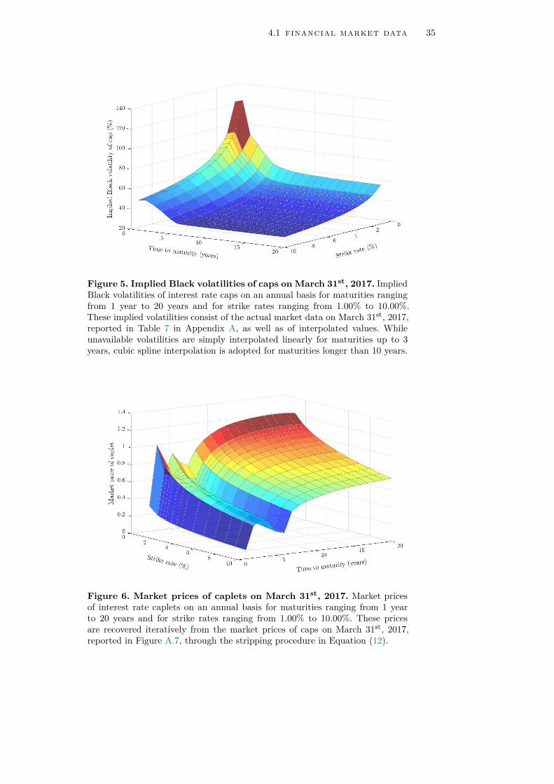
4.1 financial market data 35
Figure 5. Implied Black volatilities of caps on March 31st, 2017. ImpliedBlack volatilities of interest rate caps on an annual basis for maturities rangingfrom 1 year to 20 years and for strike rates ranging from 1.00% to 10.00%.These implied volatilities consist of the actual market data on March 31st, 2017,reported in Table 7 in Appendix A, as well as of interpolated values. Whileunavailable volatilities are simply interpolated linearly for maturities up to 3years, cubic spline interpolation is adopted for maturities longer than 10 years.
Figure 6. Market prices of caplets on March 31st, 2017. Market pricesof interest rate caplets on an annual basis for maturities ranging from 1 yearto 20 years and for strike rates ranging from 1.00% to 10.00%. These pricesare recovered iteratively from the market prices of caps on March 31st, 2017,reported in Figure A.7, through the stripping procedure in Equation (12).
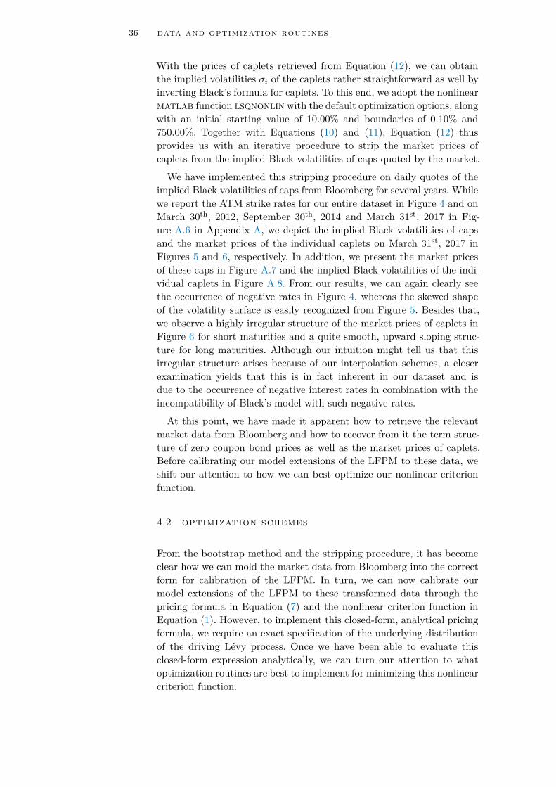
36 data and optimization routines
With the prices of caplets retrieved from Equation (12), we can obtainthe implied volatilities σi of the caplets rather straightforward as well byinverting Black’s formula for caplets. To this end, we adopt the nonlinearmatlab function lsqnonlin with the default optimization options, alongwith an initial starting value of 10.00% and boundaries of 0.10% and750.00%. Together with Equations (10) and (11), Equation (12) thusprovides us with an iterative procedure to strip the market prices ofcaplets from the implied Black volatilities of caps quoted by the market.
We have implemented this stripping procedure on daily quotes of theimplied Black volatilities of caps from Bloomberg for several years. Whilewe report the ATM strike rates for our entire dataset in Figure 4 and onMarch 30th, 2012, September 30th, 2014 and March 31st, 2017 in Fig-ure A.6 in Appendix A, we depict the implied Black volatilities of capsand the market prices of the individual caplets on March 31st, 2017 inFigures 5 and 6, respectively. In addition, we present the market pricesof these caps in Figure A.7 and the implied Black volatilities of the indi-vidual caplets in Figure A.8. From our results, we can again clearly seethe occurrence of negative rates in Figure 4, whereas the skewed shapeof the volatility surface is easily recognized from Figure 5. Besides that,we observe a highly irregular structure of the market prices of caplets inFigure 6 for short maturities and a quite smooth, upward sloping struc-ture for long maturities. Although our intuition might tell us that thisirregular structure arises because of our interpolation schemes, a closerexamination yields that this is in fact inherent in our dataset and isdue to the occurrence of negative interest rates in combination with theincompatibility of Black’s model with such negative rates.
At this point, we have made it apparent how to retrieve the relevantmarket data from Bloomberg and how to recover from it the term struc-ture of zero coupon bond prices as well as the market prices of caplets.Before calibrating our model extensions of the LFPM to these data, weshift our attention to how we can best optimize our nonlinear criterionfunction.
4.2 optimization schemes
From the bootstrap method and the stripping procedure, it has becomeclear how we can mold the market data from Bloomberg into the correctform for calibration of the LFPM. In turn, we can now calibrate ourmodel extensions of the LFPM to these transformed data through thepricing formula in Equation (7) and the nonlinear criterion function inEquation (1). However, to implement this closed-form, analytical pricingformula, we require an exact specification of the underlying distributionof the driving Lévy process. Once we have been able to evaluate thisclosed-form expression analytically, we can turn our attention to whatoptimization routines are best to implement for minimizing this nonlinearcriterion function.

4.2 optimization schemes 37
While Eberlein et al. (2016) provide us with a closed-form expression toprice individual caplets, they manage to bypass making assumptions onthe underlying distribution of the driving Lévy process in their derivation.In other words, before we can apply this pricing formula in our optimiza-tion schemes, we first need to specify the underlying distribution of thedriving Lévy process. Raible (2000) offers an extensive overview of allthe different kinds of distributions that we can implement in this case,whereas Beinhofer et al. (2011) argue that the class of Generalized Hy-perbolic (GH) distributions seems the most appropriate, since this classcan allow for an almost perfect fit to financial data. More specifically,Beinhofer et al. (2011) state that the Normal Inverse Gaussian (NIG)distribution in Barndorff-Nielsen (1998), which we can regard as a sub-class of the class of GH distributions, typically already provides sufficientflexibility to fit financial data while containing less parameters than themore general GH distribution. In addition, Eberlein and Kluge (2007)state that this class of distributions is in fact so flexible that we do noteven have to consider multi-dimensional driving processes, but that aone-dimensional Lévy process is already sufficient. We therefore incorpo-rate one-dimensional NIG distributed Lévy processes in the calibrationof our model extensions of the LFPM to the market prices of caplets.
The NIG distribution constitutes a class of distributions with four pa-rameters, which was first proposed by Barndorff-Nielsen (1995). Whilethis distribution formally depends on four parameters in total, Kluge(2005) argues that one of the parameters is irrelevant for the pricing of op-tions and can therefore be arbitrarily set to zero. Morales and Schoutens(2003) and Rydberg (1997) demonstrate that we can, in this case, repre-sent the Brownian component cNIG and the Lévy measure F T ∗
NIG(dx) ofthe driving Lévy process in terms of merely three parameters under theNIG distribution, namely bycNIG = 0
F T∗
NIG(dx) = ϑκπ|x|K1(κ|x|) exp(γx)dx
, (13)
where
Kµ(x) =∫ ∞
0uµ−1e−
12x(
1u+u)du
denotes the modified Bessel function of the second kind of order µ, andwith κ > 0, |γ| < κ and ϑ > 0. They furthermore argue that we canview this NIG distributed Lévy process as a pure jump process with aninfinite number of small jumps, since it has a Brownian component of zero.More importantly, though, by means of the specification in Equation (13),we are now able to implement our closed-form expression for pricingindividual caplets.
At this point, we are able to evaluate our nonlinear criterion functionin Equation (1) through Equations (7) and (13). The only part that wehave left unspecified up until now, is how we can best minimize this cri-

38 data and optimization routines
terion function in terms of the model parameters. We therefore adoptthe nonlinear matlab function lsqnonlin to evaluate the expression inEquation (1), and to optimize over the corresponding model parameters.Moreover, to allow for an efficient calibration of our model extensions ona daily basis, we adopt the trapezoidal method to numerically approxi-mate the three integrals in Equation (7). We can implement this methodquite easily through the matlab function trapz, with the optimizationoptions specified in Table 8 in Appendix B. With this numerical approx-imation, we manage to significantly ease our computational burden andto ensure that the LFPM retains its tractability.
However, note that this optimization routine might be sensitive to itsinitial starting values, since our criterion function could have multiplelocal minima. To resolve this issue, we therefore first perform our non-linear optimization scheme for different starting values and boundariestogether with simulated annealing, which offers a more global optimiza-tion scheme than lsqnonlin at the expense of a higher computationalburden. This, in turn, allows us to find the estimated parameters thatmatch the smallest value of our criterion function and to obtain some-what more sophisticated starting values for our calibrations. As a result,we adopt the initial starting values and boundaries reported in Table 9 inAppendix B in the calibrations of our model extensions with lsqnonlin.Even though incorporating different starting values and boundaries doesnot ensure us that we in fact acquire the global minimum of our nonlinearcriterion function, it does make our optimization routine somewhat lesssensitive to its initial starting values and more robust to local minima. Byadopting this optimization scheme, we can therefore calibrate our modelextensions of the LFPM to actual market data on caps and assess theirmodel performance.In this chapter we have explained how to retrieve the relevant market
data for calibrating the LFPM and how to transform these data into thecorrect form for our optimization routines. Besides that, we have alsodiscussed what distribution is the most appropriate for the driving Lévyprocess, and how we can best optimize our nonlinear criterion functionin terms of the transformed data and this distribution.
5EMPIR ICAL PERFORMANCE ANALYS I S
Now that we have been able to acquire the relevant market prices ofinterest rate caplets, we can actually calibrate our model extensions ofthe LFPM. In these calibrations, we have paid special attention not onlyto the goodness-of-fit, the parameter stability and the out-of-sample pric-ing performance of each model extension, but also to the effect that thetype of deterministic volatility function might have on these performancecriteria. Besides that, we have focused on the piecewise homogeneity re-striction in our calibrations, where we have assumed that each piecewisehomogeneous process follows the NIG distribution.
In this chapter we present the results of our empirical performanceanalysis of the LFPM, and provide an interpretation of these results. Tobegin with, we first present some preliminary results of these calibrationsin the next section, which enables us to assess the goodness-of-fit of ourmodel extensions.
5.1 goodness-of-fit
Implementing the relevant market data on March 31st, 2017 and our op-timization methodology described in the previous chapter, we obtain thecaplet prices of each model extension and their pricing errors. Together,this allows us to deduce the goodness-of-fit of each separate model exten-sion, with deterministic as well as with random breakpoints. While wedisplay the goodness-of-fit for each model extension in Table 2 and thecalibrated parameters in Table 10 in Appendix B, we present the capletprices of each model extension and their respective absolute pricing errorsin terms of the implied Black volatilities in Figures 7 and 8, respectively.Although the differences between all eight model extensions seem rather
modest, two of our model extensions appear to be superior to the others.To begin with, we observe from Table 2 that the LFPM with the LEVspecification slightly outperforms the other volatility functions on March31st, 2017.
39
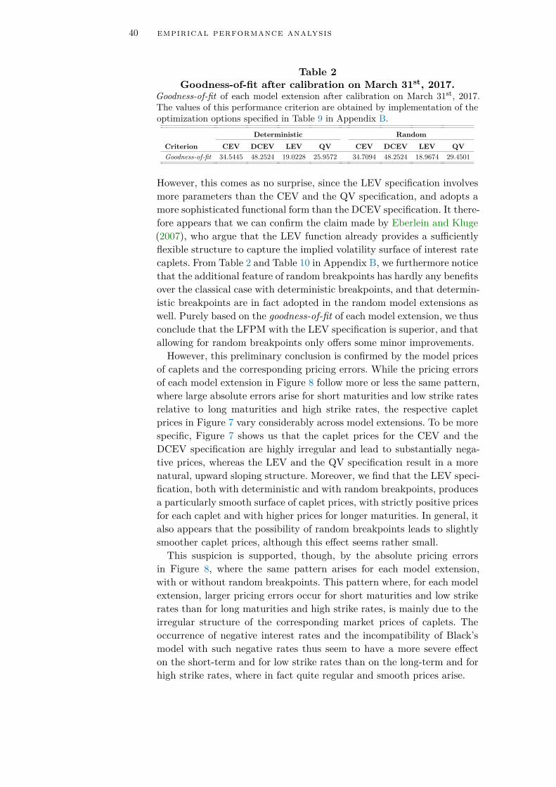
40 empirical performance analysis
Table 2Goodness-of-fit after calibration on March 31st, 2017.
Goodness-of-fit of each model extension after calibration on March 31st, 2017.The values of this performance criterion are obtained by implementation of theoptimization options specified in Table 9 in Appendix B.
Deterministic RandomCriterion CEV DCEV LEV QV CEV DCEV LEV QVGoodness-of-fit 34.5445 48.2524 19.0228 25.9572 34.7094 48.2524 18.9674 29.4501
However, this comes as no surprise, since the LEV specification involvesmore parameters than the CEV and the QV specification, and adopts amore sophisticated functional form than the DCEV specification. It there-fore appears that we can confirm the claim made by Eberlein and Kluge(2007), who argue that the LEV function already provides a sufficientlyflexible structure to capture the implied volatility surface of interest ratecaplets. From Table 2 and Table 10 in Appendix B, we furthermore noticethat the additional feature of random breakpoints has hardly any benefitsover the classical case with deterministic breakpoints, and that determin-istic breakpoints are in fact adopted in the random model extensions aswell. Purely based on the goodness-of-fit of each model extension, we thusconclude that the LFPM with the LEV specification is superior, and thatallowing for random breakpoints only offers some minor improvements.However, this preliminary conclusion is confirmed by the model prices
of caplets and the corresponding pricing errors. While the pricing errorsof each model extension in Figure 8 follow more or less the same pattern,where large absolute errors arise for short maturities and low strike ratesrelative to long maturities and high strike rates, the respective capletprices in Figure 7 vary considerably across model extensions. To be morespecific, Figure 7 shows us that the caplet prices for the CEV and theDCEV specification are highly irregular and lead to substantially nega-tive prices, whereas the LEV and the QV specification result in a morenatural, upward sloping structure. Moreover, we find that the LEV speci-fication, both with deterministic and with random breakpoints, producesa particularly smooth surface of caplet prices, with strictly positive pricesfor each caplet and with higher prices for longer maturities. In general, italso appears that the possibility of random breakpoints leads to slightlysmoother caplet prices, although this effect seems rather small.This suspicion is supported, though, by the absolute pricing errors
in Figure 8, where the same pattern arises for each model extension,with or without random breakpoints. This pattern where, for each modelextension, larger pricing errors occur for short maturities and low strikerates than for long maturities and high strike rates, is mainly due to theirregular structure of the corresponding market prices of caplets. Theoccurrence of negative interest rates and the incompatibility of Black’smodel with such negative rates thus seem to have a more severe effecton the short-term and for low strike rates than on the long-term and forhigh strike rates, where in fact quite regular and smooth prices arise.

5.1 goodness-of-fit 41
(a) CEV - Deterministic (b) CEV - Random
(c) DCEV - Deterministic (d) DCEV - Random
(e) LEV - Deterministic (f) LEV - Random
(g) QV - Deterministic (h) QV - Random
Figure 7. Caplet prices of each model extension after calibration onMarch 31st, 2017. Prices of individual interest rate caplets of each modelextension for maturities ranging from 1 year to 20 years and for strike ratesranging from 1.00% to 10.00%. The resulting prices are obtained after calibrationof the respective model extension to the market data on March 31st, 2017.

42 empirical performance analysis
(a) CEV - Deterministic (b) CEV - Random
(c) DCEV - Deterministic (d) DCEV - Random
(e) LEV - Deterministic (f) LEV - Random
(g) QV - Deterministic (h) QV - Random
Figure 8. Absolute caplet pricing errors of each model extension aftercalibration on March 31st, 2017. Absolute pricing errors of individual inter-est rate caplets of each model extension for maturities ranging from 1 year to 20years and for strike rates ranging from 1.00% to 10.00%. The resulting absolutepricing errors are expressed in implied Black volatilities and are obtained aftercalibration of the respective model extension to the market data on March 31st,2017.

5.2 parameter stability 43
Based upon the resulting caplet prices of each model extension and thecorresponding pricing errors, we can therefore confirm our earlier conclu-sion that the LFPM with the LEV specification is indeed superior, andthat allowing for random breakpoints does in fact only offer some minorimprovements.However, it remains of interest whether this conclusion depends heavily
on the date for which our model extensions are calibrated, and whetherwe arrive at the same conclusion after assessing the parameter stabilityof all eight model extensions. With this in mind, we focus on historicallycalibrating each model extension in the analysis of our next section, wherewe address the two aforementioned questions.
5.2 parameter stability
Even though the LFPM with the LEV specification has proven to besuperior to our other volatility functions, we have based this conclusionsolely on the calibrations on a single date and on the goodness-of-fit.However, it might turn out that we find significantly different results if weperform our calibrations on other dates, or that the resulting parameterestimates of the LEV specification are extremely volatile in comparisonto the other model extensions. In other words, before we can present awell-founded conclusion, we should conduct further research into thesequestions. To achieve this, we assess and discuss the parameter stabilityof our model extensions on March 30th, 2012 up until March 31st, 2017.By adopting the same optimization strategy as in the previous section
and by implementing the relevant market data on March 30th, 2012 upuntil March 31st, 2017, we manage to obtain the caplet prices of all eightmodel extensions and their absolute pricing errors. This, in turn, allowsus to quantify the parameter stability of each individual model extension,with both deterministic and random breakpoints, by assessing the stan-dard deviations of the resulting parameter estimates. In addition, we alsoinvestigate whether these calibrations lead to any substantial changes inthe resulting model prices. To this end, we present the parameter stabilityof each model extension separately in Table 3, whereas we report the cor-responding average parameter estimates and the average goodness-of-fittogether with its volatility in Tables 11 and 12 in Appendix B, respec-tively. Moreover, we display the average caplet prices of each model exten-sion in Figure B.1 in Appendix B, the volatilities of these caplet prices inFigure B.2, the respective average absolute pricing errors of each modelextension in terms of the implied Black volatilities in Figure B.3 and thevolatilities of these pricing errors in Figure B.4.
While our calibrations tend to indicate that two model extensions areagain superior to the others, we now do in fact find somewhat differentresults. From the average goodness-of-fit and its volatility in Table 11 inAppendix B, for instance, we observe that each model extension has aconsiderably worse fit to the market data than on March 31st, 2017, andthat these model fits experience huge amounts of volatility.
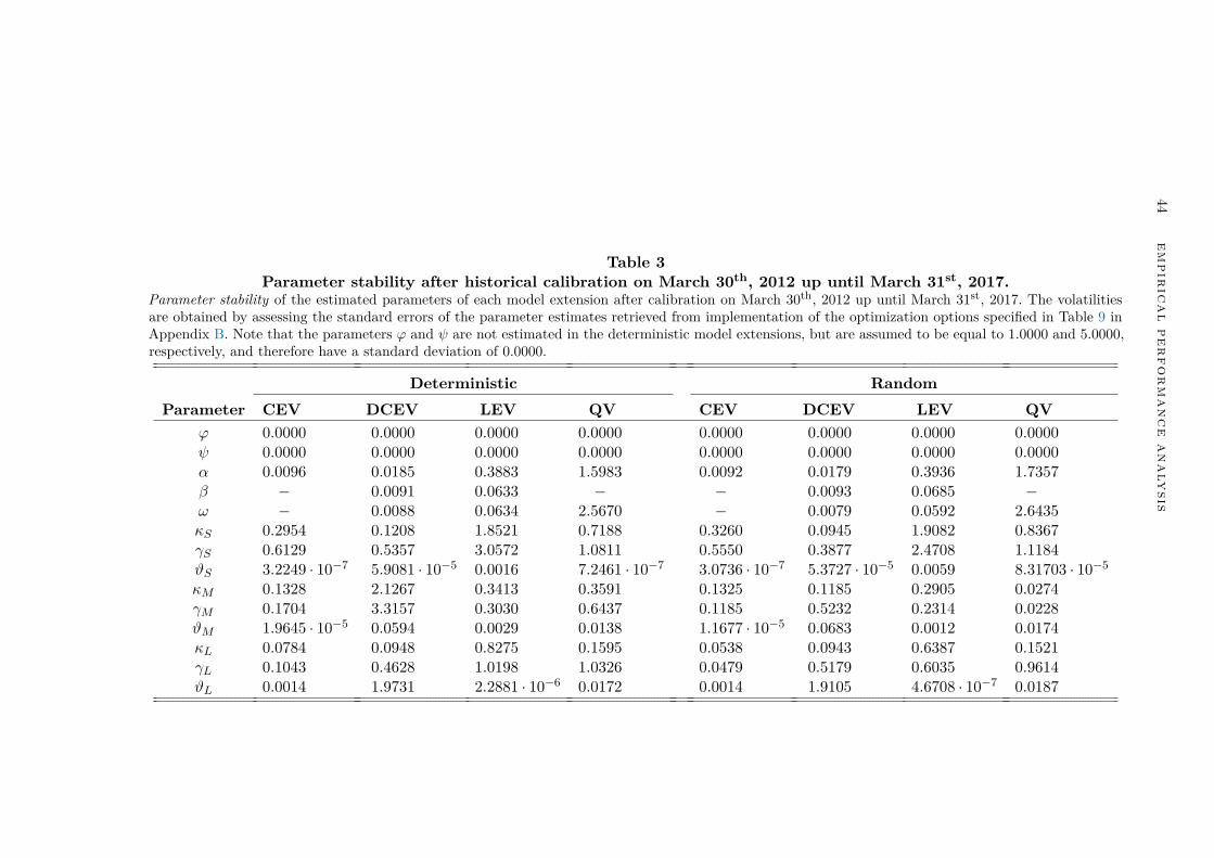
44em
pirica
lper
for
ma
nce
an
aly
sis
Table 3Parameter stability after historical calibration on March 30th, 2012 up until March 31st, 2017.
Parameter stability of the estimated parameters of each model extension after calibration on March 30th, 2012 up until March 31st, 2017. The volatilitiesare obtained by assessing the standard errors of the parameter estimates retrieved from implementation of the optimization options specified in Table 9 inAppendix B. Note that the parameters ϕ and ψ are not estimated in the deterministic model extensions, but are assumed to be equal to 1.0000 and 5.0000,respectively, and therefore have a standard deviation of 0.0000.
Deterministic RandomParameter CEV DCEV LEV QV CEV DCEV LEV QV
ϕ 0.0000 0.0000 0.0000 0.0000 0.0000 0.0000 0.0000 0.0000ψ 0.0000 0.0000 0.0000 0.0000 0.0000 0.0000 0.0000 0.0000α 0.0096 0.0185 0.3883 1.5983 0.0092 0.0179 0.3936 1.7357β − 0.0091 0.0633 − − 0.0093 0.0685 −ω − 0.0088 0.0634 2.5670 − 0.0079 0.0592 2.6435κS 0.2954 0.1208 1.8521 0.7188 0.3260 0.0945 1.9082 0.8367γS 0.6129 0.5357 3.0572 1.0811 0.5550 0.3877 2.4708 1.1184ϑS 3.2249 · 10−7 5.9081 · 10−5 0.0016 7.2461 · 10−7 3.0736 · 10−7 5.3727 · 10−5 0.0059 8.31703 · 10−5
κM 0.1328 2.1267 0.3413 0.3591 0.1325 0.1185 0.2905 0.0274γM 0.1704 3.3157 0.3030 0.6437 0.1185 0.5232 0.2314 0.0228ϑM 1.9645 · 10−5 0.0594 0.0029 0.0138 1.1677 · 10−5 0.0683 0.0012 0.0174κL 0.0784 0.0948 0.8275 0.1595 0.0538 0.0943 0.6387 0.1521γL 0.1043 0.4628 1.0198 1.0326 0.0479 0.5179 0.6035 0.9614ϑL 0.0014 1.9731 2.2881 · 10−6 0.0172 0.0014 1.9105 4.6708 · 10−7 0.0187

5.2 parameter stability 45
A closer examination of the market data reveals that this vast decreasein model fit is due to the irregular pattern inherent in the market pricesof short-term interest rate caplets. In other words, even though the LEVspecification and the DCEV specification seem to substantially outper-form the other volatility functions, all model extensions appear to beunsuccessful in appropriately incorporating this irregularity in the mar-ket prices of caplets. Our results on both the parameter stability of eachmodel extension in Table 3 and on the means of the estimated parame-ters in Table 12 in Appendix B seem to furthermore support this claim.From the parameter stability of our eight model extensions, we are ableto conclude that the resulting parameter estimates are, overall, quite sta-ble. Together with the means of these estimated parameters, this suggeststhat we can expect to obtain, on average, more or less the same structureof caplet prices for each model extension as on March 31st, 2017.
We find confirmation of this expectation in the actual caplet prices ofeach model extension. From Figures B.1 and B.2 in Appendix B, for exam-ple, we observe that we indeed obtain, on average, qualitatively the samecaplet prices for each model extension as on March 31st, 2017, and thatthese caplet prices are in fact the most volatile on the short-term. More-over, the possibility of random breakpoints again does not significantlyaffect our results, since deviating from the deterministic breakpoints onlyoffers some marginal improvements in terms of the goodness-of-fit. How-ever, our calibrations do seem to result in a somewhat less smooth struc-ture of caplet prices for the LEV specification than on March 31st, 2017,although it does still lead to strictly positive prices and preserves the up-ward sloping relationship with respect to the time to maturity. Nonethe-less, the LEV specification remains the superior model extension, sincethe LEV specification ensures the strictly positive structure of capletprices and turns out to produce the least volatile caplet prices.
Similarly, the average absolute pricing errors and their volatilities leadto qualitatively the same results, and deliver support for the aforemen-tioned conclusion as well. The average absolute pricing errors in Fig-ure B.3, for instance, display almost no discrepancy across model exten-sions and follow the same pattern as on March 31st, 2017. The argumentbrought forward by Beinhofer et al. (2011) that the class of GH distri-butions already provides enough flexibility to fit financial data, thereforeseems to uphold in our analysis, since we obtain more or less the samepricing errors for each model extension. Besides that, the volatilities ofthese pricing errors in Figure B.4 indeed exhibit a degree of variationalong the time to maturity. In other words, we do in fact observe sub-stantially larger pricing errors for short maturities than for long maturi-ties, as a result of the irregularity inherent in the market data. However,since we are mainly concerned with longer times to maturity from a riskmanagement perspective, this does not pose any severe issues. Based onour historical calibrations and on the parameter stability, we thus notonly confirm our preliminary conclusion that the LEV specification issuperior to the other model extensions and best to adopt in an ALM
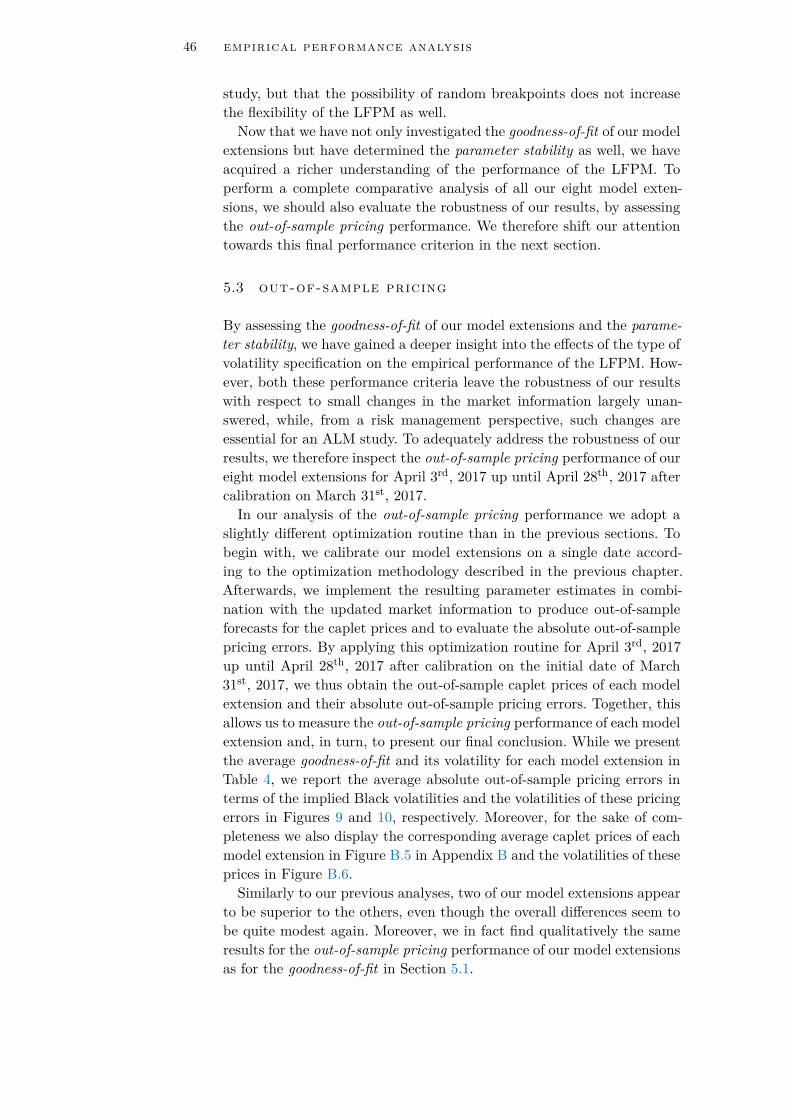
46 empirical performance analysis
study, but that the possibility of random breakpoints does not increasethe flexibility of the LFPM as well.Now that we have not only investigated the goodness-of-fit of our model
extensions but have determined the parameter stability as well, we haveacquired a richer understanding of the performance of the LFPM. Toperform a complete comparative analysis of all our eight model exten-sions, we should also evaluate the robustness of our results, by assessingthe out-of-sample pricing performance. We therefore shift our attentiontowards this final performance criterion in the next section.
5.3 out-of-sample pricing
By assessing the goodness-of-fit of our model extensions and the parame-ter stability, we have gained a deeper insight into the effects of the type ofvolatility specification on the empirical performance of the LFPM. How-ever, both these performance criteria leave the robustness of our resultswith respect to small changes in the market information largely unan-swered, while, from a risk management perspective, such changes areessential for an ALM study. To adequately address the robustness of ourresults, we therefore inspect the out-of-sample pricing performance of oureight model extensions for April 3rd, 2017 up until April 28th, 2017 aftercalibration on March 31st, 2017.In our analysis of the out-of-sample pricing performance we adopt a
slightly different optimization routine than in the previous sections. Tobegin with, we calibrate our model extensions on a single date accord-ing to the optimization methodology described in the previous chapter.Afterwards, we implement the resulting parameter estimates in combi-nation with the updated market information to produce out-of-sampleforecasts for the caplet prices and to evaluate the absolute out-of-samplepricing errors. By applying this optimization routine for April 3rd, 2017up until April 28th, 2017 after calibration on the initial date of March31st, 2017, we thus obtain the out-of-sample caplet prices of each modelextension and their absolute out-of-sample pricing errors. Together, thisallows us to measure the out-of-sample pricing performance of each modelextension and, in turn, to present our final conclusion. While we presentthe average goodness-of-fit and its volatility for each model extension inTable 4, we report the average absolute out-of-sample pricing errors interms of the implied Black volatilities and the volatilities of these pricingerrors in Figures 9 and 10, respectively. Moreover, for the sake of com-pleteness we also display the corresponding average caplet prices of eachmodel extension in Figure B.5 in Appendix B and the volatilities of theseprices in Figure B.6.Similarly to our previous analyses, two of our model extensions appear
to be superior to the others, even though the overall differences seem tobe quite modest again. Moreover, we in fact find qualitatively the sameresults for the out-of-sample pricing performance of our model extensionsas for the goodness-of-fit in Section 5.1.

5.3 out-of-sample pricing 47
Table 4Out-of-sample pricing performance after historical calibration.Out-of-sample pricing performance for April 3rd, 2017 up until April 28th, 2017in terms of the average goodness-of-fit of each model extension as well as itsstandard deviation after calibration on March 31st, 2017. The values of this per-formance criterion are obtained by implementation of the optimization optionsspecified in Table 9 in Appendix B.
Deterministic RandomCriterion CEV DCEV LEV QV CEV DCEV LEV QVAverage goodness-of-fit 40.3654 51.1501 23.8000 29.5975 39.5650 51.1501 24.6024 35.8822Standard deviation 6.5067 7.5479 8.1418 5.4990 6.2354 7.5479 8.6370 5.6975
From Table 4, we, for instance, observe that the LFPM with the LEVspecification, in general, slightly outperforms the other volatility func-tions in terms of the goodness-of-fit. More specifically, our results indicatethat the LFPM with the CEV and the DCEV specification again resultin a much worse fit than the LEV specification and that the QV functionproduces only a slightly worse fit. In addition, we find that the LEV speci-fication tends to lead to the most volatile goodness-of-fit, whereas the QVspecification introduces the most stable goodness-of-fit. We furthermoreobserve that, in contrast to our analysis in Section 5.1, the possibility ofrandom breakpoints now typically leads to a worse goodness-of-fit andto a larger volatility of this fit, and that this relation seems to be partic-ularly persistent for the LFPM with the LEV and the QV specification.However, these differences appear to arise due to the flexibility that theadditional parameters in the functional form of the volatility functionand in the Lévy measure of the driving process offer. Despite these draw-backs, the LFPM with the LEV specification continues to be the superiormodel extension, although allowing for random breakpoints now seemsto come at a considerable cost.Besides the goodness-of-fit, we also find qualitatively the same patterns
in the out-of-sample caplet prices of each model extension and their ab-solute pricing errors as in the calibrations on the initial date of our fore-casting period. While the average absolute pricing errors of each modelextension and the volatilities of these pricing errors in Figures 9 and 10,respectively, all follow approximately the same pattern, the structure ofthe average caplet prices in Figure B.5 in Appendix B is again quite ir-regular. To be more specific, we again observe that the caplet prices forthe CEV and the DCEV specification display, on average, a high degreeof irregularity and lead to considerably negative prices, whereas the LEVand the QV specification both produce a more natural, upward slopingstructure of caplet prices. Moreover, it turns out that the LEV specifica-tion, with deterministic as well as with random breakpoints, also providesthe smoothest surface of out-of-sample caplet prices, with strictly posi-tive prices for each caplet and with higher prices for longer maturities.Likewise, we find that the possibility of random breakpoints allows forslightly smoother out-of-sample caplet prices as well, although this effectappears to be minuscule at best.

48 empirical performance analysis
(a) CEV - Deterministic (b) CEV - Random
(c) DCEV - Deterministic (d) DCEV - Random
(e) LEV - Deterministic (f) LEV - Random
(g) QV - Deterministic (h) QV - Random
Figure 9. Average absolute out-of-sample caplet pricing errors of eachmodel extension after calibration on March 31st, 2017. Average absoluteout-of-sample pricing errors of individual interest rate caplets of each modelextension for maturities ranging from 1 year to 20 years and for strike ratesranging from 1.00% to 10.00%. The resulting average absolute out-of-samplepricing errors are expressed in implied Black volatilities and are obtained aftercalibration of the respective model extension to the market data on March 31st,2017 for April 3rd, 2017 up until April 28th, 2017.
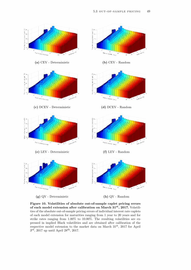
5.3 out-of-sample pricing 49
(a) CEV - Deterministic (b) CEV - Random
(c) DCEV - Deterministic (d) DCEV - Random
(e) LEV - Deterministic (f) LEV - Random
(g) QV - Deterministic (h) QV - Random
Figure 10. Volatilities of absolute out-of-sample caplet pricing errorsof each model extension after calibration on March 31st, 2017. Volatili-ties of the absolute out-of-sample pricing errors of individual interest rate capletsof each model extension for maturities ranging from 1 year to 20 years and forstrike rates ranging from 1.00% to 10.00%. The resulting volatilities are ex-pressed in implied Black volatilities and are obtained after calibration of therespective model extension to the market data on March 31st, 2017 for April3rd, 2017 up until April 28th, 2017.
50 empirical performance analysis
In addition, the volatilities of these caplet prices in Figure B.6 in Ap-pendix B are all rather modest and exhibit an upward sloping relation-ship with respect to the time to maturity. The DCEV specification fur-thermore seems to be the most stable in terms of the resulting capletprices, but since the volatilities of the out-of-sample caplet prices are allremarkably small, this result is essentially negligible.In a similar manner, we obtain the average absolute pricing errors to-
gether with the volatilities of these pricing errors in Figures 9 and 10,respectively, which barely vary across model extensions. For all modelextensions we in fact find that, on average, large absolute pricing errorstend to arise for short maturities and low strikes rates relative to longmaturities and high strike rates. This is again due to the irregular struc-ture of the corresponding market prices of caplets that arises as a resultof the occurrence of negative interest rates and the incompatibility ofBlack’s model with such negative rates. We furthermore observe in Fig-ure 10 that the volatilities of these pricing errors are actually larger forlong maturities than for short maturities, which does not come as a sur-prise since we already found that the out-of-sample caplet prices tend tobe more volatile for long maturities than for short maturities. All thingsconsidered, though, each of our eight model extensions seem to lead tosimilar out-of-sample pricing errors, and a comparison based on thesepricing errors does therefore not contribute much to the differentiationof our model extensions in terms of their empirical performance.After a comprehensive performance analysis of our eight model exten-
sions of the LFPM, we have gained a richer understanding of how thechoice of volatility specification affects the empirical performance of theLFPM. More specifically, we have investigated and discussed how welleach functional form of the volatility specification, with deterministic aswell as with random breakpoints, fits the actual market data on interestrate caplets and how robust our results are with respect to these mar-ket data. Based on the goodness-of-fit, the parameter stability and theout-of-sample pricing performance of each model extension, we thereforeconclude that the LFPM with the LEV specification is superior to theother volatility functions, and that this model extension is best incor-porated in an ALM study with deterministic breakpoints. In the next,and also last, chapter of this thesis, we summarize the most importantfindings of our research, and conclude with some final remarks on thelimitations of our research as well as with some suggestions for futurestudies.

6SUMMARY AND CONCLUDING REMARKS
The main objective of the research in this thesis was to discover how wecan best construct and estimate a stochastic term structure model forAsset Liability Management purposes. Because of the increasing concernfor negative interest rates and the risk that this low, negative interest rateenvironment poses for financial institutions, the urgency of accountingfor the current state of financial markets has risen sharply. We thus notonly required our stochastic interest rate model to capture the pricesof popular interest rate derivatives traded in the market, but to allowfor substantially negative interest rate scenarios as well. Through theimplementation of such a stochastic term structure model in an AssetLiability Management study, financial institutions are able to addressthis interest rate risk and it therefore enables them to more globallyassess their financial stability.
As a result of an extensive literature review, we presented an overviewof state-of-the-art stochastic term structure models, where we comparedthe fundamental characteristics of these models in terms of their adequacyfor an Asset Liability Management study. This comprehensive compar-ison eventually led to the striking result that some of the most widelyadopted short-rate models in practice are in fact highly inappropriatein the negative interest rate environment that we currently observe, andthat only the Lévy Forward Price Model has appropriate characteristicsfor Asset Liability Management purposes. Further study of the Lévy For-ward Price Model resulted in the specification of eight different modelextensions. We implemented four types of deterministic volatility func-tions in these model extensions under a piecewise homogeneity restrictionon the driving one-dimensional Lévy process, with both deterministic andrandom breakpoints. The novelty of our approach was the exact param-eterization of this restriction in terms of the canonical representationsof the driving piecewise homogeneous Lévy processes. In addition, wealso introduced a concatenation of the processes in this specification tofurther enhance the smoothness of the driving process as a whole.
51

52 summary and concluding remarks
After applying a stripping procedure and the bootstrap method to ac-quire all the relevant market data, we calibrated our model extensionsof the Lévy Forward Price Model to the market prices of interest ratecaplets. These calibrations led to a comprehensive performance analy-sis of each model extension of the Lévy Forward Price Model on March30th, 2012 up until April 28th, 2017. From this extensive comparison, weconcluded that the Linear-Exponential Volatility specification yields, byfar, the best results and outperforms the other deterministic volatilityfunctions. At the foundation of this comprehensive comparison lied threeessential performance criteria, namely the goodness-of-fit, the parameterstability and the out-of-sample pricing performance of each model ex-tension. Moreover, while the possibility of random breakpoints in thepiecewise homogeneous Lévy processes seemed to offer only some minorbenefits in terms of the goodness-of-fit and essentially none in terms of theparameter stability, it in fact severely worsened the out-of-sample pricingperformance of the Linear-Exponential Volatility specification. Our com-parative analysis therefore indicated that the Lévy Forward Price Modelis best adopted in an Asset Liability Management study with the Linear-Exponential Volatility specification and with deterministic breakpoints.
The research of this thesis was primarily concerned with the goodness-of-fit, the parameter stability and the out-of-sample pricing performanceof each model extension. However, future studies could, of course, alsoevaluate somewhat more sophisticated criteria to investigate whether thiswould lead to qualitatively the same results. The jackknife resamplingmethod is one of these more sophisticated criteria, for instance, whichcan be implemented to assess the robustness of our results with respectto the inclusion of longer maturities and additional strike rates. Moreover,while we mainly focused on rather straightforward volatility functions inthis thesis, more complex approaches that involve a nonparametric kernelregression, a Principal Components Analysis or the General Method ofMoments could be adopted in further research as well. In turn, the im-plementation of such advanced volatility specifications could extend ourcomprehension of the empirical performance of the Lévy Forward PriceModel, and could be employed to validate the conclusions of the researchin this thesis. Additionally, it would be worth investigating whether theirregularity observed in the market prices of caplets would reduce if wehad a novel framework that is, unlike Black’s model, consistent with neg-ative interest rates. Such a state-of-the-art framework could enhance theempirical performance of the Lévy Forward Price Model considerably. Asa final suggestion for further research, we would recommend focusing ona sensitivity analysis of the optimization options adopted in this thesisto assess the robustness and the accuracy of our results.
All things considered, in this thesis we have discussed how financialinstitutions can best construct and estimate a stochastic term structuremodel for Asset Liability Management purposes. Our overview of state-of-the-art stochastic term structure models furthermore highlighted thefact that some of the most widely adopted short-rate models in practice

summary and concluding remarks 53
are nowadays in fact highly inappropriate for taking interest rate riskinto account. However, the relatively new and unknown Lévy ForwardPrice Model has proven to be capable of dealing with the risk that thispersistently negative interest rate environment poses in our empirical per-formance analysis. From a risk management perspective, it is thereforeof crucial importance that financial institutions abandon short-rate mod-els and introduce the Lévy Forward Price Model in their Asset LiabilityManagement studies to adequately take interest rate risk into account.


REFERENCES
Aït-Sahalia, Y. and Lo, A. W. (1998). Nonparametric estimation of state-price densities implicit in financial asset prices. The Journal of Finance,53(2):499–547.
Amin, K. I. and Morton, A. J. (1994). Implied volatility functions inarbitrage-free term structure models. Journal of Financial Economics,35(2):141–180.
Andersen, L. and Andreasen, J. (2000). Volatility skews and extensionsof the Libor market model. Applied Mathematical Finance, 7(1):1–32.
Andersen, L. B. and Brotherton-Ratcliffe, R. (2005). Extended Libormarket models with stochastic volatility. Journal of ComputationalFinance, 9(1):1–40.
Barndorff-Nielsen, O. E. (1995). Normal inverse Gaussian distributionsand the modeling of stock returns. Research Report No. 300, Depart-ment of Theoretical Statistics, Aarhus University, Aarhus, Denmark.
Barndorff-Nielsen, O. E. (1998). Processes of normal inverse Gaussiantype. Finance and Stochastics, 2(1):41–68.
Beinhofer, M., Eberlein, E., Janssen, A., and Polley, M. (2011). Correla-tions in Lévy interest rate models. Quantitative Finance, 11(9):1315–1327.
Björk, T. (2007). Topics in interest rate theory. Handbooks in OperationsResearch and Management Science, 15:377–435.
Black, F. (1976). The pricing of commodity contracts. Journal of Finan-cial Economics, 3(1-2):167–179.
Black, F. and Scholes, M. (1973). The pricing of options and corporateliabilities. Journal of Political Economy, 81(3):637–654.
Brace, A., Gatarek, D., and Musiela, M. (1997). The market model ofinterest rate dynamics. Mathematical Finance, 7(2):127–155.
Brigo, D. and Mercurio, F. (2007). Interest rate models – Theory andpractice: With smile, inflation and credit. Springer, Berlin.
55

56 References
Brigo, D., Mercurio, F., and Morini, M. (2005). The LIBOR model dy-namics: Approximations, calibration and diagnostics. European Jour-nal of Operational Research, 163(1):30–51.
Buraschi, A. and Jackwerth, J. (2001). The price of a smile: Hedging andspanning in option markets. Review of Financial Studies, 14(2):495–527.
Cox, J. C., Ingersoll Jr, J. E., and Ross, S. A. (1985). A theory of theterm structure of interest rates. Econometrica, 53(2):385–407.
Cox, J. C. and Ross, S. A. (1976). The valuation of options for alternativestochastic processes. Journal of Financial Economics, 3(1-2):145–166.
De Jong, F., Driessen, J., and Pelsser, A. (2001). Libor Market Modelsversus Swap Market Models for pricing interest rate derivatives: Anempirical analysis. European Finance Review, 5(3):201–237.
De Kort, J. and Vellekoop, M. (2016). Term structure extrapolationand asymptotic forward rates. Insurance: Mathematics and Economics,67:107–119.
Driessen, J., Klaassen, P., and Melenberg, B. (2003). The performanceof multi-factor term structure models for pricing and hedging capsand swaptions. The Journal of Financial and Quantitative Analysis,38(3):635–672.
Eberlein, E., Eddahbi, M., and Lalaoui Ben Cherif, S. M. (2016). Optionpricing and sensitivity analysis in the Lévy forward process model. InInnovations in Derivatives Markets, pages 285–313. Springer, Cham.
Eberlein, E., Jacod, J., and Raible, S. (2005). Lévy term structure models:No-arbitrage and completeness. Finance and Stochastics, 9(1):67–88.
Eberlein, E. and Kluge, W. (2007). Calibration of Lévy term struc-ture models. In Advances in Mathematical Finance, pages 147–172.Birkhäuser, Boston.
Eberlein, E. and Özkan, F. (2005). The Lévy LIBOR model. Financeand Stochastics, 9(3):327–348.
Errais, E. and Mercurio, F. (2005). Yes, Libor models can capture interestrate derivatives skew: A simple modelling approach. Working PaperNo. 680621, Society for Computational Economics, Washington, D.C.,United States of America.
Filipović, D. (2009). Term-structure models: A graduate course. Springer,Berlin.
Garía, R. L. (2013). Construction and analysis of fixed-income volatilityindices. PhD thesis, University of Castile-La Mancha, Ciudad Real,Spain.

References 57
Glau, K., Grbac, Z., and Papapantoleon, A. (2016). A unified view of LI-BOR models. In Advanced Modelling in Mathematical Finance, pages423–452. Springer, Cham.
Gupta, A. and Subrahmanyam, M. G. (2005). Pricing and hedging inter-est rate options: Evidence from cap–floor markets. Journal of Banking& Finance, 29(3):701–733.
Heath, D., Jarrow, R., and Morton, A. (1992). Bond pricing and the termstructure of interest rates: A new methodology for contingent claimsvaluation. Econometrica, 60(1):77–105.
Henrard, M. (2005). Swaptions: 1 price, 10 deltas, and... 6 1/2 gammas.Wilmott Magazine, 6:48–57.
Hilber, N., Reich, N., Schwab, C., and Winter, C. (2009). Numericalmethods for Lévy processes. Finance and Stochastics, 13(4):471–500.
Hull, J. and White, A. (1990). Pricing interest-rate-derivative securities.Review of Financial Studies, 3(4):573–592.
Jacod, J. and Shiryaev, A. N. (2003). Limit theorems for stochastic pro-cesses. Springer, Berlin.
Jamshidian, F. (1997). LIBOR and swap market models and measures.Finance and Stochastics, 1(4):293–330.
Jarrow, R. A. (2009). The term structure of interest rates. The AnnualReview of Financial Economics, 1(1):69–96.
Joshi, M. S., Rebonato, R., et al. (2003). A displaced-diffusion stochasticvolatility LIBOR market model: Motivation, definition and implemen-tation. Quantitative Finance, 3(6):458–469.
Kallsen, J. and Shiryaev, A. N. (2002). The cumulant process and Esscher’s change of measure. Finance and Stochastics, 6(4):397–428.
Kluge, W. (2005). Time-inhomogeneous Lévy processes in interest rateand credit risk models. PhD thesis, University of Freiburg, Freiburg,Germany.
Kluge, W. and Papapantoleon, A. (2009). On the valuation of composi-tions in Lévy term structure models. Quantitative Finance, 9(8):951–959.
Leippold, M. and Strømberg, J. (2014). Time-changed Lévy LIBORmarket model: Pricing and joint estimation of the cap surface andswaption cube. Journal of Financial Economics, 111(1):224–250.
Lemke, W. (2006). Term structure modeling and estimation in a statespace framework. Springer, Berlin.

58 References
Miltersen, K. R., Sandmann, K., and Sondermann, D. (1997). Closedform solutions for term structure derivatives with log-normal interestrates. The Journal of Finance, 52(1):409–430.
Morales, M. and Schoutens, W. (2003). A risk model driven by Lévy pro-cesses. Applied Stochastic Models in Business and Industry, 19(2):147–167.
Nelson, C. R. and Siegel, A. F. (1987). Parsimonious modeling of yieldcurves. Journal of Business, 60(4):473–489.
Papapantoleon, A. (2010). Old and new approaches to LIBOR modeling.Statistica Neerlandica, 64(3):257–275.
Raible, S. (2000). Lévy processes in finance: Theory, numerics, and em-pirical facts. PhD thesis, University of Freiburg, Freiburg, Germany.
Rebonato, R. (2004). Review Paper. Interest–rate term–structure pricingmodels: A review. InMathematical, Physical and Engineering Sciences,pages 667–728. The Royal Society, London.
Rydberg, T. H. (1997). The normal inverse Gaussian Lévy process: Sim-ulation and approximation. Communications in Statistics: StochasticModels, 13(4):887–910.
Schmidt, W. M. (2011). Interest rate term structure modelling. EuropeanJournal of Operational Research, 214(1):1–14.
Svensson, L. E. (1994). Estimating and interpreting forward interestrates: Sweden 1992-1994. Working Paper No. 579, Institute for Inter-national Economic Studies, Stockholm, Sweden.
Vasicek, O. (1977). An equilibrium characterization of the term structure.Journal of Financial Economics, 5(2):177–188.
Veronesi, P. (2010). Fixed income securities: Valuation, risk and riskmanagement. John Wiley & Sons, Hoboken.
Zuhlsdorff, C. (2001). The pricing of derivatives on assets with quadraticvolatility. Applied Mathematical Finance, 8(4):235–262.

AHISTORICAL MARKET DATA
Table 5Market swap rates from Bloomberg on March 31st, 2017.
Values of the market swap rates quoted on March 31st, 2017 by Bloomberg.All market swap rates have the 6-month EURIBOR rate as their underlyingindex and are, apart from the swap rate with a maturity of half a year, annuallycompounded. These values are obtained through their corresponding tickers andfields from Bloomberg. Source: Bloomberg.
Maturity (years) Ticker Field Swap rate (%)0.5 EUSWF CMPL Curncy PX_LAST −0.24501 EUSA1 CMPL Curncy PX_LAST −0.21842 EUSA2 CMPL Curncy PX_LAST −0.12953 EUSA3 CMPL Curncy PX_LAST −0.03904 EUSA4 CMPL Curncy PX_LAST 0.06805 EUSA5 CMPL Curncy PX_LAST 0.18206 EUSA6 CMPL Curncy PX_LAST 0.30357 EUSA7 CMPL Curncy PX_LAST 0.42508 EUSA8 CMPL Curncy PX_LAST 0.54609 EUSA9 CMPL Curncy PX_LAST 0.662010 EUSA10 CMPL Curncy PX_LAST 0.764011 EUSA11 CMPL Curncy PX_LAST 0.863012 EUSA12 CMPL Curncy PX_LAST 0.948513 EUSA13 CMPL Curncy PX_LAST 1.022514 EUSA14 CMPL Curncy PX_LAST 1.087515 EUSA15 CMPL Curncy PX_LAST 1.142516 EUSA16 CMPL Curncy PX_LAST 1.187017 EUSA17 CMPL Curncy PX_LAST 1.227018 EUSA18 CMPL Curncy PX_LAST 1.256519 EUSA19 CMPL Curncy PX_LAST 1.282520 EUSA20 CMPL Curncy PX_LAST 1.304521 EUSA21 CMPL Curncy PX_LAST 1.321522 EUSA22 CMPL Curncy PX_LAST 1.335523 EUSA23 CMPL Curncy PX_LAST 1.347524 EUSA24 CMPL Curncy PX_LAST 1.357525 EUSA25 CMPL Curncy PX_LAST 1.365526 EUSA26 CMPL Curncy PX_LAST 1.372027 EUSA27 CMPL Curncy PX_LAST 1.377528 EUSA28 CMPL Curncy PX_LAST 1.382529 EUSA29 CMPL Curncy PX_LAST 1.386530 EUSA30 CMPL Curncy PX_LAST 1.390035 EUSA35 CMPL Curncy PX_LAST 1.400540 EUSA40 CMPL Curncy PX_LAST 1.400545 EUSA45 CMPL Curncy PX_LAST 1.357150 EUSA50 CMPL Curncy PX_LAST 1.3605
59

60 historical market data
Figure A.1. Swap curve on March 30th, 2012, September 30th, 2014and on March 31st, 2017. Swap curves on a semi-annual basis for maturitiesranging from half a year to 50 years. The red dots represent the actual mar-ket data on March 30th, 2012, September 30th, 2014 and on March 31st, 2017,whereas the blue curves denote the interpolated swap curves after cubic splineinterpolation.
Figure A.2. Implied discount factors on March 30th, 2012, September30th, 2014 and on March 31st, 2017. Discount factors on a semi-annualbasis for maturities ranging from half a year to 50 years. These discount factorsare extracted from the swap curves on March 30th, 2012, September 30th, 2014and on March 31st, 2017 in Figure A.1 through implementation of the bootstrapmethod in Equation (8).
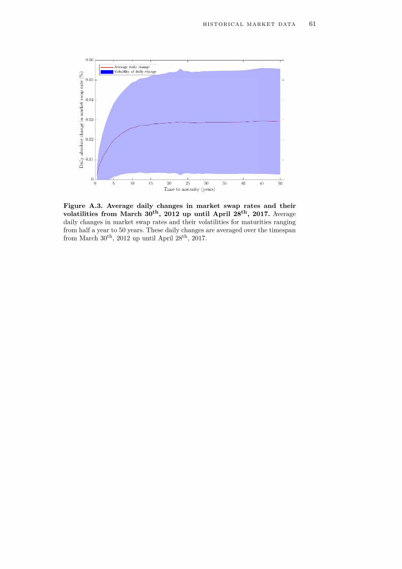
historical market data 61
Figure A.3. Average daily changes in market swap rates and theirvolatilities from March 30th, 2012 up until April 28th, 2017. Averagedaily changes in market swap rates and their volatilities for maturities rangingfrom half a year to 50 years. These daily changes are averaged over the timespanfrom March 30th, 2012 up until April 28th, 2017.

62h
istor
ical
ma
rk
etd
ata
Table 6Tickers and fields of implied Black volatilities of caps from Bloomberg.
Tickers of the implied Black volatilities of interest rate caps quoted by Bloomberg. All caps have the 6-month EURIBOR rate as their underlying index,apart from the caps with a maturity of 1 year and 2 years which are linked to the 3-month EURIBOR rate. These tickers all require the suffix ‘BBIRCurncy’, together with the field ‘PX_LAST’ to obtain the implied Black volatilities of caps from Bloomberg.
Strike rate
Maturity (years) ATM 1.00% 1.75% 2.00% 2.25% 2.50% 3.00% 3.50% 4.00% 5.00% 6.00% 7.00% 8.00% 9.00% 10.00%1 EUCV1 EUCF101 EUCF1751 EUCF201 EUCF2251 EUCF251 EUCF301 EUCF351 EUCF401 EUCF501 EUCF601 EUCF701 EUCF801 EUCF901 EUCF0012 EUCV2 EUCF102 EUCF1752 EUCF202 EUCF2252 EUCF252 EUCF302 EUCF352 EUCF402 EUCF502 EUCF602 EUCF702 EUCF802 EUCF902 EUCF0023 EUCV3 EUCF103 EUCF1753 EUCF203 EUCF2253 EUCF253 EUCF303 EUCF353 EUCF403 EUCF503 EUCF603 EUCF703 EUCF803 EUCF903 EUCF0034 EUCV4 EUCF104 EUCF1754 EUCF204 EUCF2254 EUCF254 EUCF304 EUCF354 EUCF404 EUCF504 EUCF604 EUCF704 EUCF804 EUCF904 EUCF0045 EUCV5 EUCF105 EUCF1755 EUCF205 EUCF2255 EUCF255 EUCF305 EUCF355 EUCF405 EUCF505 EUCF605 EUCF705 EUCF805 EUCF905 EUCF0056 EUCV6 EUCF106 EUCF1756 EUCF206 EUCF2256 EUCF256 EUCF306 EUCF356 EUCF406 EUCF506 EUCF606 EUCF706 EUCF806 EUCF906 EUCF0067 EUCV7 EUCF107 EUCF1757 EUCF207 EUCF2257 EUCF257 EUCF307 EUCF357 EUCF407 EUCF507 EUCF607 EUCF707 EUCF807 EUCF907 EUCF0078 EUCV8 EUCF108 EUCF1758 EUCF208 EUCF2258 EUCF258 EUCF308 EUCF358 EUCF408 EUCF508 EUCF608 EUCF708 EUCF808 EUCF908 EUCF0089 EUCV9 EUCF109 EUCF1759 EUCF209 EUCF2259 EUCF259 EUCF309 EUCF359 EUCF409 EUCF509 EUCF609 EUCF709 EUCF809 EUCF909 EUCF00910 EUCV10 EUCF1010 EUCF1710 EUCF2010 EUCF2210 EUCF2510 EUCF3010 EUCF3510 EUCF4010 EUCF5010 EUCF6010 EUCF7010 EUCF8010 EUCF9010 EUCF001012 EUCV12 EUCF1012 EUCF1712 EUCF2012 EUCF2212 EUCF2512 EUCF3012 EUCF3512 EUCF4012 EUCF5012 EUCF6012 EUCF7012 EUCF8012 EUCF9012 EUCF001215 EUCV15 EUCF1015 EUCF1715 EUCF2015 EUCF2215 EUCF2515 EUCF3015 EUCF3515 EUCF4015 EUCF5015 EUCF6015 EUCF7015 EUCF8015 EUCF9015 EUCF001520 EUCV20 EUCF1020 EUCF1720 EUCF2020 EUCF2220 EUCF220 EUCF3020 EUCF3520 EUCF4020 EUCF5020 EUCF6020 EUCF7020 EUCF8020 EUCF9020 EUCF0020

histo
rica
lm
ar
ket
data
63
Table 7Implied Black volatilities of caps from Bloomberg on March 31st, 2017.
Values of the implied Black volatilities of interest rate caps quoted on March 31st, 2017 by Bloomberg. All caps have the 6-month EURIBOR rate as theirunderlying index, apart from the caps with a maturity of 1 year and 2 years which are linked to the 3-month EURIBOR rate. These values are obtainedthrough their corresponding tickers and fields reported in Table 6 from Bloomberg. Source: Bloomberg.
Strike rate
Maturity (years) ATM 1.00% 1.75% 2.00% 2.25% 2.50% 3.00% 3.50% 4.00% 5.00% 6.00% 7.00% 8.00% 9.00% 10.00%1 N/A 125.01 94.83 89.62 85.43 81.94 76.40 72.14 68.71 63.42 59.46 56.32 53.74 51.57 49.692 N/A 126.92 97.22 91.82 87.45 83.81 78.03 73.59 70.01 64.53 60.45 57.23 54.59 52.37 50.473 165.33 93.09 79.46 76.43 73.83 71.54 67.73 64.60 61.99 57.79 54.53 51.89 49.70 47.82 46.204 147.93 84.17 71.15 68.30 65.89 63.80 60.34 57.56 55.26 51.59 48.74 46.42 44.48 47.81 41.365 113.19 74.73 62.57 59.92 57.67 55.73 52.51 49.92 47.78 44.39 41.81 39.74 38.04 36.59 35.346 92.06 67.18 55.95 53.51 51.43 49.63 46.65 44.26 42.29 39.18 36.81 34.92 33.37 32.06 30.947 80.17 63.93 53.47 51.20 49.27 47.61 44.85 42.65 40.84 37.99 35.84 34.12 32.70 31.50 30.478 72.84 62.26 52.35 50.20 48.37 46.79 44.19 42.10 40.38 37.68 35.62 33.97 32.59 31.43 30.419 72.84 61.27 51.74 49.67 47.91 46.39 43.88 41.86 40.19 37.56 35.54 33.91 32.56 31.40 30.3910 64.53 60.64 51.37 49.36 47.64 46.16 43.71 41.73 40.09 37.50 35.51 33.89 32.54 31.39 30.3812 60.16 59.88 50.97 49.02 47.36 45.92 43.53 41.60 40.00 37.45 35.47 33.87 32.52 31.37 30.3615 56.75 59.32 50.68 48.79 47.14 45.76 43.42 41.52 39.94 37.42 35.45 33.85 32.51 31.36 30.3520 54.56 58.91 50.48 48.63 47.04 45.66 43.35 41.48 39.92 37.40 35.44 33.85 32.51 31.36 30.36

64 historical market data
Figure A.4. Average daily changes in implied Black volatilities of capsfrom March 30th, 2012 up until April 28th, 2017. Average daily changesin implied Black volatilities of interest rate caps for maturities ranging from 1year to 20 years and for strike rates ranging from 1.00% to 10.00%. These dailychanges are averaged over the timespan from March 30th, 2012 up until April28th, 2017.
Figure A.5. Volatilities of daily changes in implied Black volatilitiesof caps from March 30th, 2012 up until April 28th, 2017. Volatilities ofthe daily changes in implied Black volatilities of interest rate caps for maturitiesranging from 1 year to 20 years and for strike rates ranging from 1.00% to 10.00%.These volatilities represent the standard deviations in the daily changes over thetimespan from March 30th, 2012 up until April 28th, 2017.

historical market data 65
Figure A.6. ATM strike rates on March 30th, 2012, September 30th,2014 and on March 31st, 2017. ATM strike rates on an annual basis formaturities ranging from 1 year to 20 years. These strike rates are computedthrough Equation (11) with the implied discount factors from Figure A.2 onMarch 30th, 2012, September 30th, 2014 and on March 31st, 2017.
Figure A.7. Market prices of caps on March 31st, 2017. Market pricesof interest rate caps on an annual basis for maturities ranging from 1 year to20 years and for strike rates ranging from 1.00% to 10.00%. These prices arerecovered from the actual market data on March 31st, 2017, reported in Figure 5,through Equation (10).
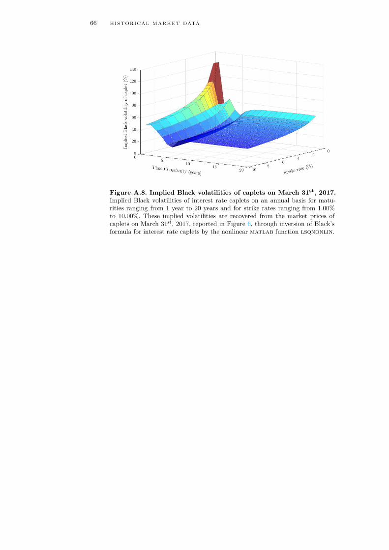
66 historical market data
Figure A.8. Implied Black volatilities of caplets on March 31st, 2017.Implied Black volatilities of interest rate caplets on an annual basis for matu-rities ranging from 1 year to 20 years and for strike rates ranging from 1.00%to 10.00%. These implied volatilities are recovered from the market prices ofcaplets on March 31st, 2017, reported in Figure 6, through inversion of Black’sformula for interest rate caplets by the nonlinear matlab function lsqnonlin.
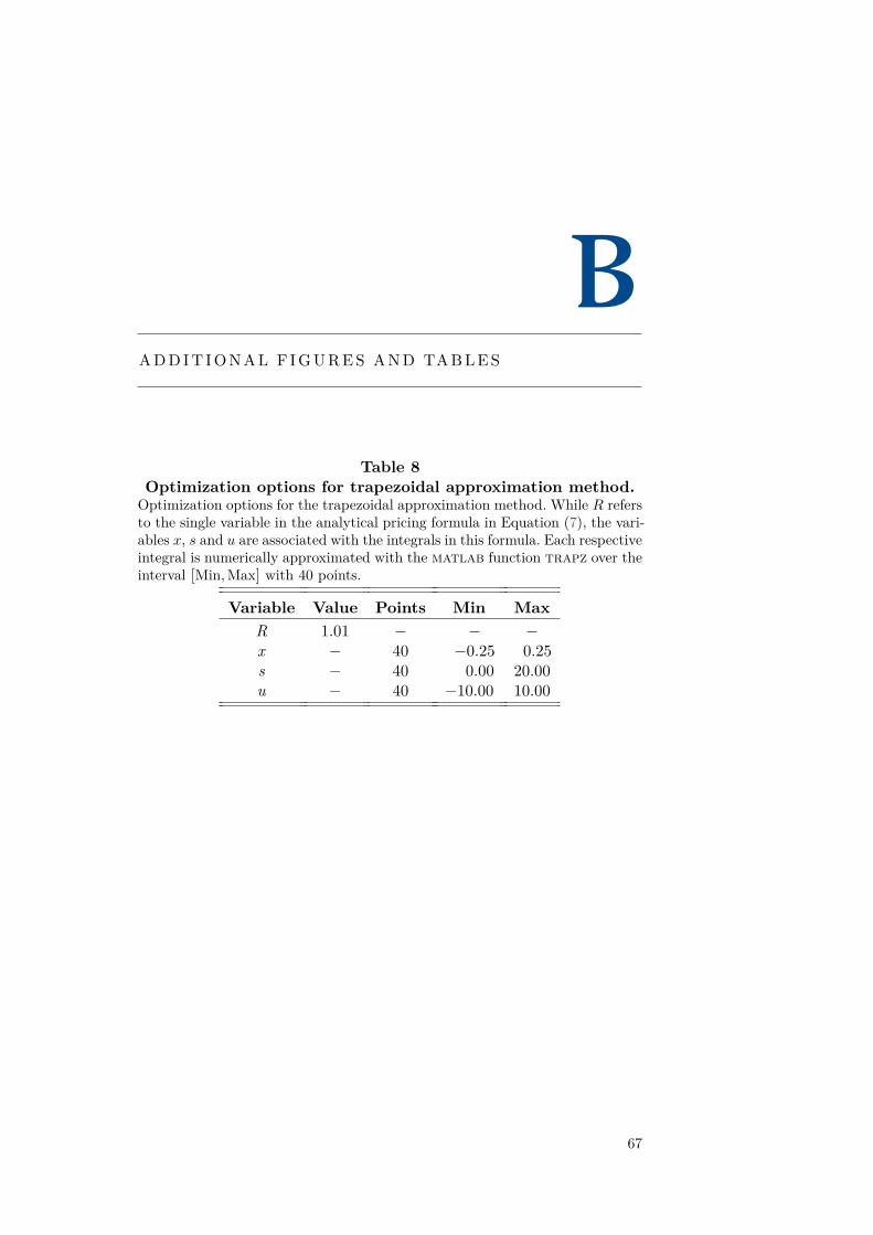
BADDIT IONAL F IGURES AND TABLES
Table 8Optimization options for trapezoidal approximation method.
Optimization options for the trapezoidal approximation method. While R refersto the single variable in the analytical pricing formula in Equation (7), the vari-ables x, s and u are associated with the integrals in this formula. Each respectiveintegral is numerically approximated with the matlab function trapz over theinterval [Min,Max] with 40 points.
Variable Value Points Min MaxR 1.01 − − −x − 40 −0.25 0.25s − 40 0.00 20.00u − 40 −10.00 10.00
67

68a
dd
ition
al
figu
res
an
dta
bles
Table 9Optimization options for calibration scheme.
Optimization options for the calibration scheme. While the initial starting values are reported for every parameter of each model extension, the correspondingboundaries are given as well. The nonlinear matlab function lsqnonlin is initialized with these settings, together with an optimality tolerance of 0.0010,a function tolerance of 0.0100 and a step tolerance of 0.1000.
Initial starting value Lower bound Upper boundParameter CEV DCEV LEV QV CEV DCEV LEV QV CEV DCEV LEV QV
ϕ 1.0000 1.0000 1.0000 1.0000 0.0000 0.0000 0.0000 0.0000 20.0000 20.0000 20.0000 20.0000ψ 5.0000 5.0000 5.0000 5.0000 0.0000 0.0000 0.0000 0.0000 20.0000 20.0000 20.0000 20.0000α 0.3211 0.3383 10.3067 14.5703 0.1500 0.1500 5.0000 −25.0000 0.6000 0.5500 15.0000 25.0000β − 1.0000 + 10−7 0.8327 − − 1.0000 + 10−10 −2.0000 − − 2.0000 2.0000 −ω − −0.1731 0.3239 21.6398 − −5.0000 −1.5000 1.0000 · 10−10 − 5.0000 1.5000 50.0000κS 14.2021 26.7585 24.1624 26.6181 10.2500 + 10−10 15.0000 + 10−10 20.0000 + 10−10 15.0000 + 10−10 20.0000 30.0000 35.0000 35.0000γS −1.8322 15.1687 0.0594 2.0123 −10.2500 −20.0000 −15.0000 −15.0000 10.2500 20.0000 15.0000 15.0000ϑS 7.3965 · 10−7 1.2650 · 10−4 3.1664 · 10−5 1.3323 · 10−6 1.0000 · 10−10 1.0000 · 10−10 1.0000 · 10−10 1.0000 · 10−10 20.0000 15.0000 5.0000 5.0000κM 11.3013 13.5470 8.5205 7.0012 11.3000 + 10−10 11.0000 + 10−10 6.0000 + 10−10 7.0000 + 10−10 25.0000 25.0000 25.0000 20.0000γM −11.3000− 10−5 −5.2569 −3.6307 −6.9973 −11.3000 −11.0000 −6.0000 −7.0000 11.3000 11.0000 6.0000 7.0000ϑM 1.0000 · 10−5 1.0958 · 10−10 5.9454 · 10−5 4.6491 · 10−8 1.0000 · 10−10 1.0000 · 10−10 1.0000 · 10−10 1.0000 · 10−10 20.0000 5.0000 5.0000 5.0000κL 5.9250 + 10−5 4.8500 15.8443 8.2312 5.9250 + 10−10 4.8250 + 10−10 7.5000 + 10−10 7.50000 + 10−10 15.0000 15.0000 20.0000 25.0000γL −5.9250 + 10−5 −4.8106 2.8799 −0.1307 −5.9250 −4.8250 −7.5000 −7.5000 5.9250 4.8250 7.5000 7.5000ϑL 0.0048 13.5084 4.1269 · 10−7 0.0328 1.0000 · 10−10 1.0000 · 10−10 1.0000 · 10−10 1.0000 · 10−10 20.0000 20.0000 5.0000 5.0000
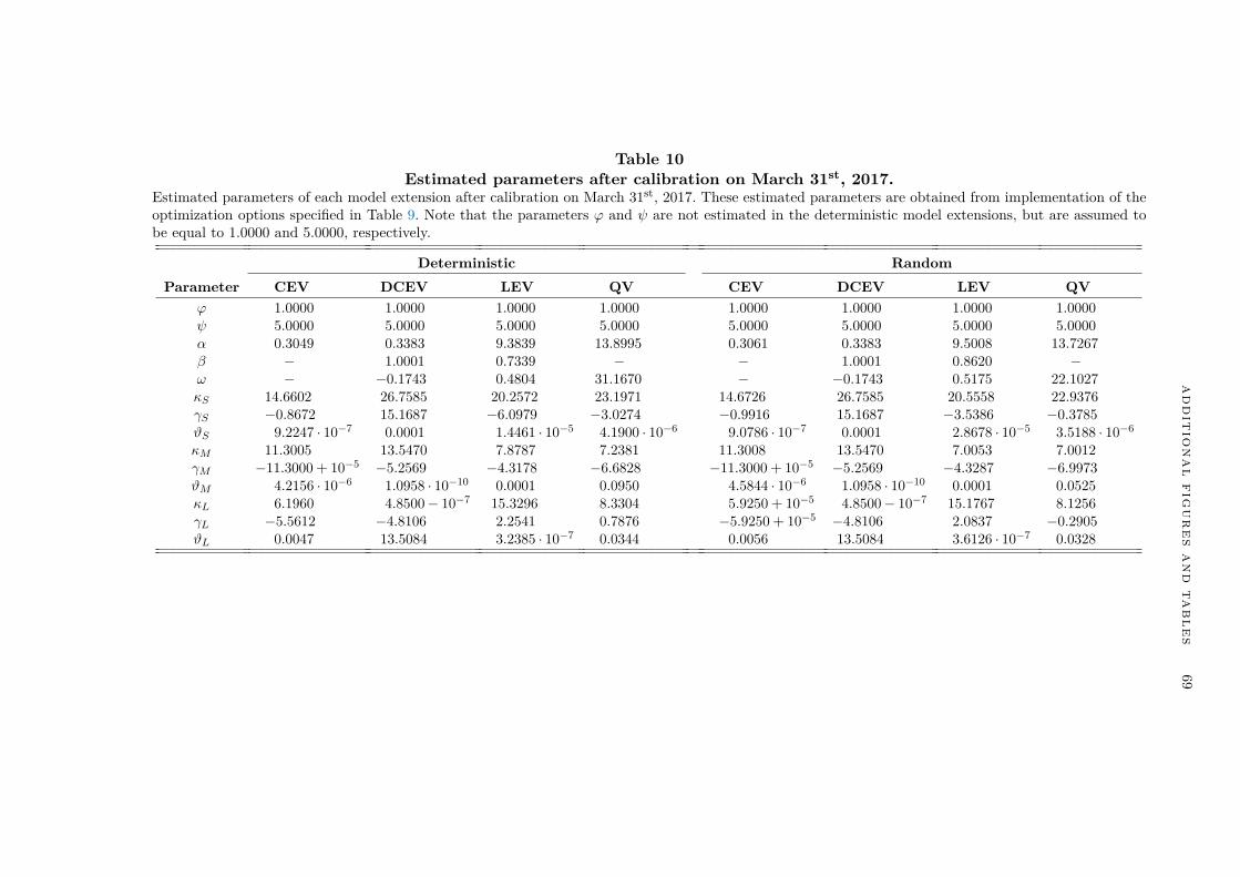
ad
ditio
na
lfig
ur
esa
nd
tables
69
Table 10Estimated parameters after calibration on March 31st, 2017.
Estimated parameters of each model extension after calibration on March 31st, 2017. These estimated parameters are obtained from implementation of theoptimization options specified in Table 9. Note that the parameters ϕ and ψ are not estimated in the deterministic model extensions, but are assumed tobe equal to 1.0000 and 5.0000, respectively.
Deterministic RandomParameter CEV DCEV LEV QV CEV DCEV LEV QV
ϕ 1.0000 1.0000 1.0000 1.0000 1.0000 1.0000 1.0000 1.0000ψ 5.0000 5.0000 5.0000 5.0000 5.0000 5.0000 5.0000 5.0000α 0.3049 0.3383 9.3839 13.8995 0.3061 0.3383 9.5008 13.7267β − 1.0001 0.7339 − − 1.0001 0.8620 −ω − −0.1743 0.4804 31.1670 − −0.1743 0.5175 22.1027κS 14.6602 26.7585 20.2572 23.1971 14.6726 26.7585 20.5558 22.9376γS −0.8672 15.1687 −6.0979 −3.0274 −0.9916 15.1687 −3.5386 −0.3785ϑS 9.2247 · 10−7 0.0001 1.4461 · 10−5 4.1900 · 10−6 9.0786 · 10−7 0.0001 2.8678 · 10−5 3.5188 · 10−6
κM 11.3005 13.5470 7.8787 7.2381 11.3008 13.5470 7.0053 7.0012γM −11.3000 + 10−5 −5.2569 −4.3178 −6.6828 −11.3000 + 10−5 −5.2569 −4.3287 −6.9973ϑM 4.2156 · 10−6 1.0958 · 10−10 0.0001 0.0950 4.5844 · 10−6 1.0958 · 10−10 0.0001 0.0525κL 6.1960 4.8500− 10−7 15.3296 8.3304 5.9250 + 10−5 4.8500− 10−7 15.1767 8.1256γL −5.5612 −4.8106 2.2541 0.7876 −5.9250 + 10−5 −4.8106 2.0837 −0.2905ϑL 0.0047 13.5084 3.2385 · 10−7 0.0344 0.0056 13.5084 3.6126 · 10−7 0.0328
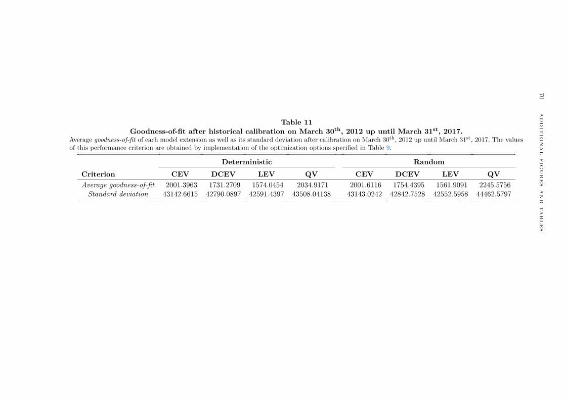
70a
dd
ition
al
figu
res
an
dta
bles
Table 11Goodness-of-fit after historical calibration on March 30th, 2012 up until March 31st, 2017.
Average goodness-of-fit of each model extension as well as its standard deviation after calibration on March 30th, 2012 up until March 31st, 2017. The valuesof this performance criterion are obtained by implementation of the optimization options specified in Table 9.
Deterministic RandomCriterion CEV DCEV LEV QV CEV DCEV LEV QVAverage goodness-of-fit 2001.3963 1731.2709 1574.0454 2034.9171 2001.6116 1754.4395 1561.9091 2245.5756Standard deviation 43142.6615 42790.0897 42591.4397 43508.04138 43143.0242 42842.7528 42552.5958 44462.5797

ad
ditio
na
lfig
ur
esa
nd
tables
71
Table 12Means of estimated parameters after historical calibration on March 30th, 2012 up until March 31st, 2017.
Means of the estimated parameters of each model extension after calibration on March 30th, 2012 up until March 31st, 2017. These means are obtained byaveraging the parameter estimates retrieved from implementation of the optimization options specified in Table 9. Note that the parameters ϕ and ψ arenot estimated in the deterministic model extensions, but are assumed to be equal to 1.0000 and 5.0000, respectively.
Deterministic RandomParameter CEV DCEV LEV QV CEV DCEV LEV QV
ϕ 1.0000 1.0000 1.0000 1.0000 1.0000 1.0000 1.0000 1.0000ψ 5.0000 5.0000 5.0000 5.0000 5.0000 5.0000 5.0000 5.0000α 0.3193 0.3418 10.1067 14.2062 0.3194 0.3408 10.1035 14.1420β − 1.0026 0.8389 − − 1.0021 0.8362 −ω − −0.1753 0.3399 21.5972 − −0.1747 0.3405 21.6672κS 14.2318 26.7611 23.4078 26.4073 14.2329 26.7581 23.3999 26.3639γS −1.7718 15.1541 −1.1556 1.6928 −1.7782 15.1537 −0.8709 1.6633ϑS 8.1893 · 10−7 0.0002 0.0001 1.5017 · 10−6 8.2399 · 10−7 0.0002 0.0003 3.8109 · 10−6
κM 11.3478 13.6050 8.4807 7.0345 11.3424 13.5462 8.4740 7.0044γM −11.2411 −5.8179 −3.6798 −6.9187 −11.2615 −5.1933 −3.6713 −6.9945ϑM 1.1457 · 10−5 0.0108 0.0001 0.0041 1.1050 · 10−5 0.0140 0.0001 0.0058κL 5.9327 4.8684 15.7523 8.1697 5.9300 4.8643 15.7828 8.1682γL −5.9143 −4.7211 2.7595 −0.4094 −5.9205 −4.7154 2.7984 −0.3859ϑL 0.0045 12.4950 4.7582 · 10−7 0.03464 0.0045 12.5085 4.1224 · 10−7 0.0352

72 additional figures and tables
(a) CEV - Deterministic (b) CEV - Random
(c) DCEV - Deterministic (d) DCEV - Random
(e) LEV - Deterministic (f) LEV - Random
(g) QV - Deterministic (h) QV - Random
Figure B.1. Average caplet prices of each model extension after cali-bration on March 30th, 2012 up until March 31st, 2017. Average pricesof individual interest rate caplets of each model extension for maturities rangingfrom 1 year to 20 years and for strike rates ranging from 1.00% to 10.00%. Theresulting average prices are obtained after calibration of the respective modelextension to the market data on March 30th, 2012 up until March 31st, 2017.

additional figures and tables 73
(a) CEV - Deterministic (b) CEV - Random
(c) DCEV - Deterministic (d) DCEV - Random
(e) LEV - Deterministic (f) LEV - Random
(g) QV - Deterministic (h) QV - Random
Figure B.2. Volatilities of caplet prices of each model extension aftercalibration on March 30th, 2012 up until March 31st, 2017. Volatilitiesof the prices of individual interest rate caplets of each model extension for matu-rities ranging from 1 year to 20 years and for strike rates ranging from 1.00% to10.00%. The resulting volatilities are obtained after calibration of the respectivemodel extension to the market data on March 30th, 2012 up until March 31st,2017.
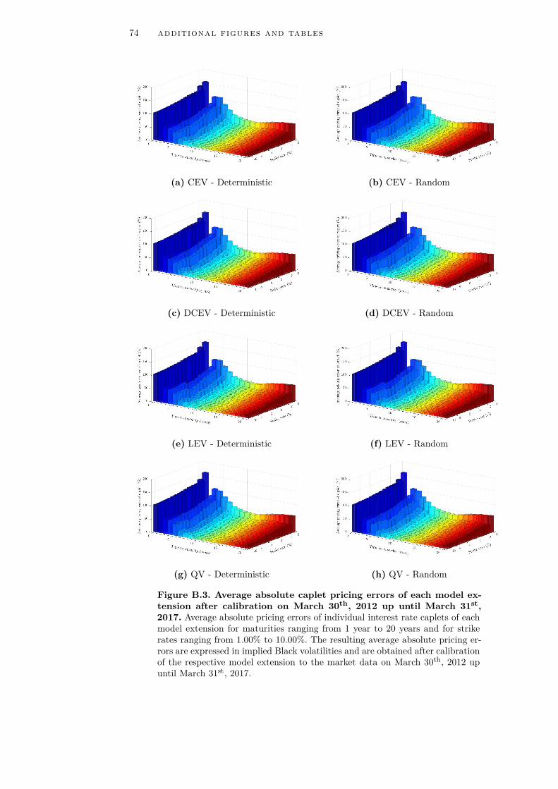
74 additional figures and tables
(a) CEV - Deterministic (b) CEV - Random
(c) DCEV - Deterministic (d) DCEV - Random
(e) LEV - Deterministic (f) LEV - Random
(g) QV - Deterministic (h) QV - Random
Figure B.3. Average absolute caplet pricing errors of each model ex-tension after calibration on March 30th, 2012 up until March 31st,2017. Average absolute pricing errors of individual interest rate caplets of eachmodel extension for maturities ranging from 1 year to 20 years and for strikerates ranging from 1.00% to 10.00%. The resulting average absolute pricing er-rors are expressed in implied Black volatilities and are obtained after calibrationof the respective model extension to the market data on March 30th, 2012 upuntil March 31st, 2017.

additional figures and tables 75
(a) CEV - Deterministic (b) CEV - Random
(c) DCEV - Deterministic (d) DCEV - Random
(e) LEV - Deterministic (f) LEV - Random
(g) QV - Deterministic (h) QV - Random
Figure B.4. Volatilities of absolute caplet pricing errors of each modelextension after calibration on March 30th, 2012 up until March 31st,2017. Volatilities of the absolute pricing errors of individual interest rate capletsof each model extension for maturities ranging from 1 year to 20 years andfor strike rates ranging from 1.00% to 10.00%. The resulting volatilities areexpressed in implied Black volatilities and are obtained after calibration of therespective model extension to the market data on March 30th, 2012 up untilMarch 31st, 2017.
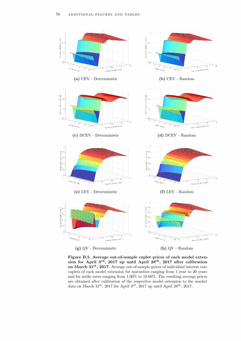
76 additional figures and tables
(a) CEV - Deterministic (b) CEV - Random
(c) DCEV - Deterministic (d) DCEV - Random
(e) LEV - Deterministic (f) LEV - Random
(g) QV - Deterministic (h) QV - Random
Figure B.5. Average out-of-sample caplet prices of each model exten-sion for April 3rd, 2017 up until April 28th, 2017 after calibrationon March 31st, 2017. Average out-of-sample prices of individual interest ratecaplets of each model extension for maturities ranging from 1 year to 20 yearsand for strike rates ranging from 1.00% to 10.00%. The resulting average pricesare obtained after calibration of the respective model extension to the marketdata on March 31st, 2017 for April 3rd, 2017 up until April 28th, 2017.

additional figures and tables 77
(a) CEV - Deterministic (b) CEV - Random
(c) DCEV - Deterministic (d) DCEV - Random
(e) LEV - Deterministic (f) LEV - Random
(g) QV - Deterministic (h) QV - Random
Figure B.6. Volatilities of out-of-sample caplet prices of each modelextension for April 3rd, 2017 up until April 28th, 2017 after calibrationon March 31st, 2017. Volatilities of the out-of-sample prices of individualinterest rate caplets of each model extension for maturities ranging from 1 yearto 20 years and for strike rates ranging from 1.00% to 10.00%. The resultingvolatilities are obtained after calibration of the respective model extension tothe market data on March 31st, 2017 for April 3rd, 2017 up until April 28th,2017.