Embed Size (px)
Citation preview
Stochastic optimization of fiber reinforcedcomposites considering uncertainties
Stochastische Optimierung der Faserparameter in Faserverbundwerkstoffenunter Bercksichtigung Unsicherheiten
DISSERTATION
Zur Erlangung des akademischen Grades einesDoktor-Ingenieur
an der Fakultat Bauingenieurwesender Bauhaus-Universitat Weimar
vorgelegt von
M.Sc. Hamid Ghasemi Meyghani(interner Doktorand)
geboren am 06. Juni 1981 in
Arak, Iran
Mentor: Prof. Dr.-Ing. Timon Rabczuk
Weimar, Mai 2016

To my wife and my little daughter ...

Acknowledgements
I would like to express my special appreciation and thanks to my advisorProf. Dr.-Ing. Timon Rabczuk for all of his supports of my Ph.D study andrelated research, for his patience, motivation, and immense knowledge. Iwould also like to thank the members of my dissertation committee: Pro-fessor Tom Lahmer and Professor Pedro Areias for generously offeringtheir time, support and guidance all over the preparation and review of thisdocument.I gratefully acknowledge three years financial support from the Ernst-Abbe-Stiftung within ”Nachwuchsforderprogramm”. I wish also espe-cially to thank Professor Stephane Bordas and Dr. Pierre Kerfriden forgranting me a worthwhile research opportunity in institute of mechanicsand advanced materials at Cardiff University. I would like to thank all ofmy research fellows there, for making my stay fruitful and enjoyable. Mysincere thanks also goes to Dr. Roberto Brighenti from the University ofParma; Dr. Jacob Muthu from the University of Witwatersrand and Dr.Roham Rafiee from the University of Tehran for all of their supports.A special thanks to my family. I would like to express my deepest gratitudeto my mother and father; to my whole family and my wife’s family for allof their supports and love. Words cannot express how grateful I am to mywife who suffered from my long evenings at the Institute; who has beensupporting me in difficult moments by her understanding, love, patience,and belief in me. Next, to my little daughter Golsa; who has been my littleshining light and inspiration.Last but not the least, thanks also go to Ms. Marlis Terber and my othercolleagues from the Institute of Structural Mechanics at Bauhaus-UniversitatWeimar for their help and friendly support.
Hamid GhasemiWeimar, GermanyMay 2016
Abstract
Briefly, the two basic questions that this research is supposed to answerare:
1. How much fiber is needed and how fibers should be distributed througha fiber reinforced composite (FRC) structure in order to obtain theoptimal and reliable structural response?
2. How do uncertainties influence the optimization results and reliabil-ity of the structure?
Giving answer to the above questions a double stage sequential optimiza-tion algorithm for finding the optimal content of short fiber reinforcementsand their distribution in the composite structure, considering uncertain de-sign parameters, is presented. In the first stage, the optimal amount of shortfibers in a FRC structure with uniformly distributed fibers is conductedin the framework of a Reliability Based Design Optimization (RBDO)problem. Presented model considers material, structural and modelinguncertainties. In the second stage, the fiber distribution optimization (with the aim to further increase in structural reliability) is performed bydefining a fiber distribution function through a Non-Uniform Rational B-Spline (NURBS) surface. The advantages of using the NURBS surfaceas a fiber distribution function include: using the same data set for theoptimization and analysis; high convergence rate due to the smoothnessof the NURBS; mesh independency of the optimal layout; no need forany post processing technique and its non-heuristic nature. The output ofstage 1 (the optimal fiber content for homogeneously distributed fibers) isconsidered as the input of stage 2. The output of stage 2 is the Reliabil-ity Index (β ) of the structure with the optimal fiber content and distribu-tion. First order reliability method (in order to approximate the limit statefunction) as well as different material models including Rule of Mixtures,Mori-Tanaka, energy-based approach and stochastic multi-scales are im-plemented in different examples. The proposed combined model is ableto capture the role of available uncertainties in FRC structures through acomputationally efficient algorithm using all sequential, NURBS and sen-sitivity based techniques. The methodology is successfully implementedfor interfacial shear stress optimization in sandwich beams and also for op-timization of the internal cooling channels in a ceramic matrix composite.

Finally, after some changes and modifications by combining IsogeometricAnalysis, level set and point wise density mapping techniques, the compu-tational framework is extended for topology optimization of piezoelectric/ flexoelectric materials.
Contents
1 Introduction 11.1 Motivation . . . . . . . . . . . . . . . . . . . . . . . . . . . . . . . . 11.2 Literature Review . . . . . . . . . . . . . . . . . . . . . . . . . . . . 31.3 Objectives of the dissertation . . . . . . . . . . . . . . . . . . . . . . 41.4 Innovations of the dissertation . . . . . . . . . . . . . . . . . . . . . 41.5 Outline . . . . . . . . . . . . . . . . . . . . . . . . . . . . . . . . . 5
2 Fundamentals of NURBS 82.1 An introduction to Isogeometric Analysis . . . . . . . . . . . . . . . 82.2 Knot vector . . . . . . . . . . . . . . . . . . . . . . . . . . . . . . . 82.3 NURBS functions and surfaces . . . . . . . . . . . . . . . . . . . . . 9
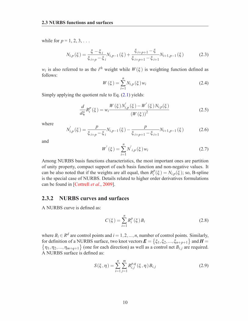
2.3.1 NURBS basis functions and derivatives . . . . . . . . . . . . 92.3.2 NURBS curves and surfaces . . . . . . . . . . . . . . . . . . 10
3 Structural reliability 123.1 Reliability assessment . . . . . . . . . . . . . . . . . . . . . . . . . . 12
3.1.1 First order reliability method (FORM) . . . . . . . . . . . . . 143.1.2 RBDO . . . . . . . . . . . . . . . . . . . . . . . . . . . . . 15
4 Optimization of fiber distribution in fiber reinforced composite 174.1 Introduction . . . . . . . . . . . . . . . . . . . . . . . . . . . . . . . 174.2 FRC homogenization methodology . . . . . . . . . . . . . . . . . . . 184.3 Definition of the optimization problem . . . . . . . . . . . . . . . . . 21
4.3.1 Objective function and optimization formulation for static prob-lems . . . . . . . . . . . . . . . . . . . . . . . . . . . . . . . 22
4.3.2 Objective function and optimization formulation for free vi-bration problems . . . . . . . . . . . . . . . . . . . . . . . . 24
4.3.3 Sensitivity analysis . . . . . . . . . . . . . . . . . . . . . . . 244.3.4 Optimization procedure . . . . . . . . . . . . . . . . . . . . 25
4.4 Case studies . . . . . . . . . . . . . . . . . . . . . . . . . . . . . . . 264.4.1 Three-point bending of a wall beam . . . . . . . . . . . . . . 27
v
CONTENTS
4.4.2 Free vibration of a beam . . . . . . . . . . . . . . . . . . . . 304.4.3 Square plate with a central circular hole under tension . . . . 31
4.5 Concluding remarks . . . . . . . . . . . . . . . . . . . . . . . . . . . 33
5 Uncertainties propagation in optimization of CNT/polymer composite 355.1 Introduction . . . . . . . . . . . . . . . . . . . . . . . . . . . . . . . 355.2 Stochastic multi-scale CNT/polymer material model . . . . . . . . . . 365.3 Metamodeling . . . . . . . . . . . . . . . . . . . . . . . . . . . . . . 39
5.3.1 Concept and application . . . . . . . . . . . . . . . . . . . . 395.3.2 Kriging method . . . . . . . . . . . . . . . . . . . . . . . . . 39
5.4 RBDO and metamodel based RBDO . . . . . . . . . . . . . . . . . . 415.5 Case studies . . . . . . . . . . . . . . . . . . . . . . . . . . . . . . . 43
5.5.1 Three-point bending of a beam . . . . . . . . . . . . . . . . . 435.5.2 Thick cylinder under radial line load . . . . . . . . . . . . . . 47
5.6 Concluding remarks . . . . . . . . . . . . . . . . . . . . . . . . . . . 53
6 Reliability and NURBS based sequential optimization approach 546.1 Introduction . . . . . . . . . . . . . . . . . . . . . . . . . . . . . . . 546.2 Double sequential stages optimization procedure . . . . . . . . . . . 546.3 Case studies . . . . . . . . . . . . . . . . . . . . . . . . . . . . . . . 57
6.3.1 Cantilever beam under static loading, verification of the model 586.3.2 Beam under three-point bending . . . . . . . . . . . . . . . . 596.3.3 Square plate with a central circular hole under tension . . . . 62
6.4 Concluding remarks . . . . . . . . . . . . . . . . . . . . . . . . . . . 63
7 Application 1: Interfacial shear stress optimization in sandwich beams 657.1 Introduction . . . . . . . . . . . . . . . . . . . . . . . . . . . . . . . 657.2 Introduction to FGM and homogenization technique . . . . . . . . . . 66
7.2.1 Rule of mixtures (ROM) method . . . . . . . . . . . . . . . . 677.2.2 Mori-Tanaka method . . . . . . . . . . . . . . . . . . . . . . 67
7.3 Material discontinuity . . . . . . . . . . . . . . . . . . . . . . . . . 687.4 Overview of optimization methodology . . . . . . . . . . . . . . . . 71
7.4.1 Adjoint sensitivity analysis . . . . . . . . . . . . . . . . . . . 727.5 Case studies . . . . . . . . . . . . . . . . . . . . . . . . . . . . . . 73
7.5.1 Verification of the IGA model . . . . . . . . . . . . . . . . . 747.5.2 Optimization case studies . . . . . . . . . . . . . . . . . . . 777.5.3 Concluding remarks . . . . . . . . . . . . . . . . . . . . . . 82
8 Application 2: Probabilistic multiconstraints optimization of cooling chan-nels in ceramic matrix composites 868.1 Introduction . . . . . . . . . . . . . . . . . . . . . . . . . . . . . . . 86
vi
CONTENTS
8.2 Thermoelastic formulation . . . . . . . . . . . . . . . . . . . . . . . 878.3 Reliability based design . . . . . . . . . . . . . . . . . . . . . . . . . 91
8.3.1 Deterministic design versus reliability based design . . . . . . 918.3.2 Probabilistic multiconstraints . . . . . . . . . . . . . . . . . 918.3.3 RBDO . . . . . . . . . . . . . . . . . . . . . . . . . . . . . 92
8.4 Adopting the double sequential stages optimization methodology . . . 928.4.1 Adjoint sensitivity analysis . . . . . . . . . . . . . . . . . . . 93
8.5 Case studies . . . . . . . . . . . . . . . . . . . . . . . . . . . . . . . 978.5.1 The first stage of the optimization . . . . . . . . . . . . . . . 978.5.2 The second stage of the optimization . . . . . . . . . . . . . . 101
8.6 Concluding remarks . . . . . . . . . . . . . . . . . . . . . . . . . . . 106
9 Application 3: A level-set based IGA formulation for topology optimiza-tion of flexoelectric materials 1079.1 Introduction . . . . . . . . . . . . . . . . . . . . . . . . . . . . . . . 1079.2 Flexoelectricity: theory and formulation . . . . . . . . . . . . . . . . 1099.3 Discretization . . . . . . . . . . . . . . . . . . . . . . . . . . . . . . 1129.4 Level Set Method (LSM) and optimization problem . . . . . . . . . . 115
9.4.1 LSM . . . . . . . . . . . . . . . . . . . . . . . . . . . . . . 1159.4.2 Optimization problem . . . . . . . . . . . . . . . . . . . . . 1179.4.3 Sensitivity analysis . . . . . . . . . . . . . . . . . . . . . . . 117
9.5 Numerical examples . . . . . . . . . . . . . . . . . . . . . . . . . . 1209.5.1 Verification of the IGA model . . . . . . . . . . . . . . . . . 1209.5.2 Topology optimization of the flexoelectric beam . . . . . . . 123
9.6 Concluding remarks . . . . . . . . . . . . . . . . . . . . . . . . . . 127
10 Conclusions 12810.1 Summary of achievements . . . . . . . . . . . . . . . . . . . . . . . 12810.2 Outlook . . . . . . . . . . . . . . . . . . . . . . . . . . . . . . . . . 131
References 132
Curriculum Vitae 140
vii
List of Figures
2.1 Different NURBS domains (a-c) and typical basis functions (d); Ap-proximating nodal values of ϕi, j defined on control points by usingNURBS surface ηp (c) . . . . . . . . . . . . . . . . . . . . . . . . . 9
3.1 Structural reliability concept . . . . . . . . . . . . . . . . . . . . . . 133.2 Graphical representation of the FORM approximation . . . . . . . . . 14
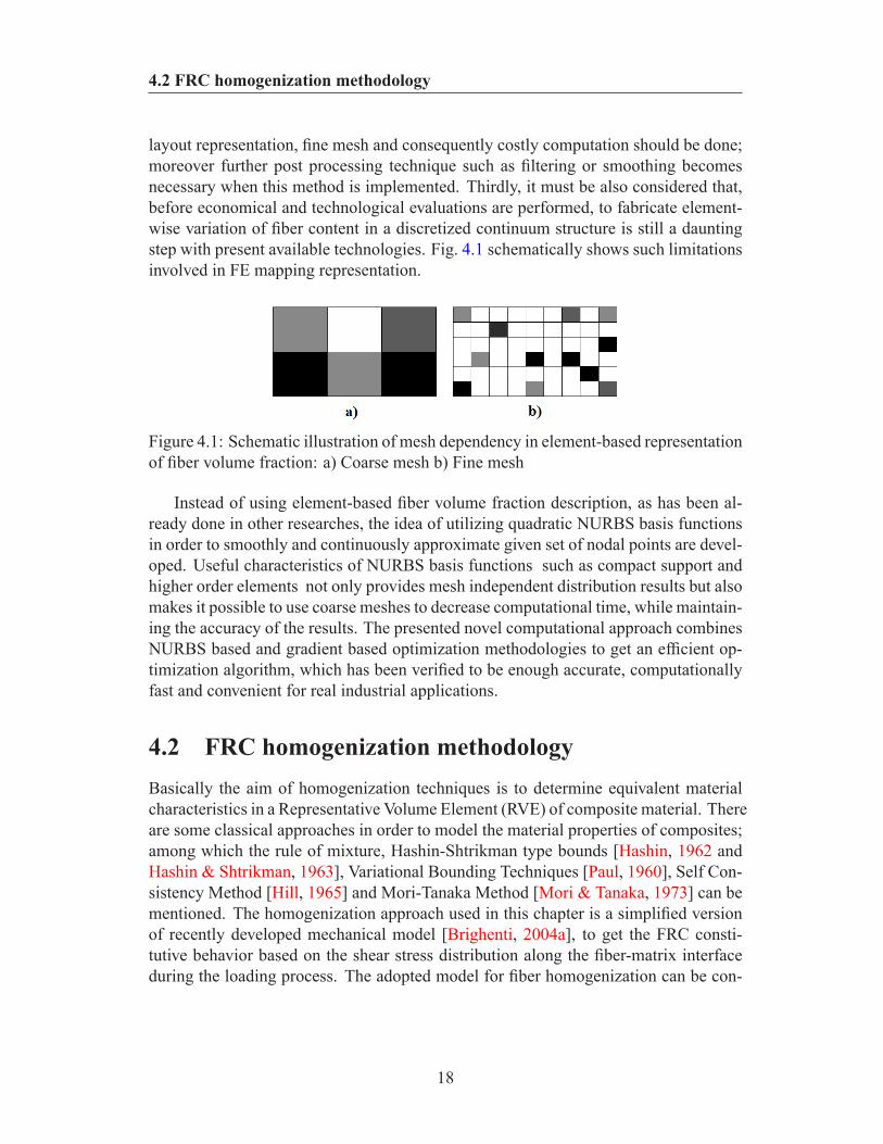
4.1 Schematic illustration of mesh dependency in element-based represen-tation of fiber volume fraction: a) Coarse mesh b) Fine mesh . . . . . 18
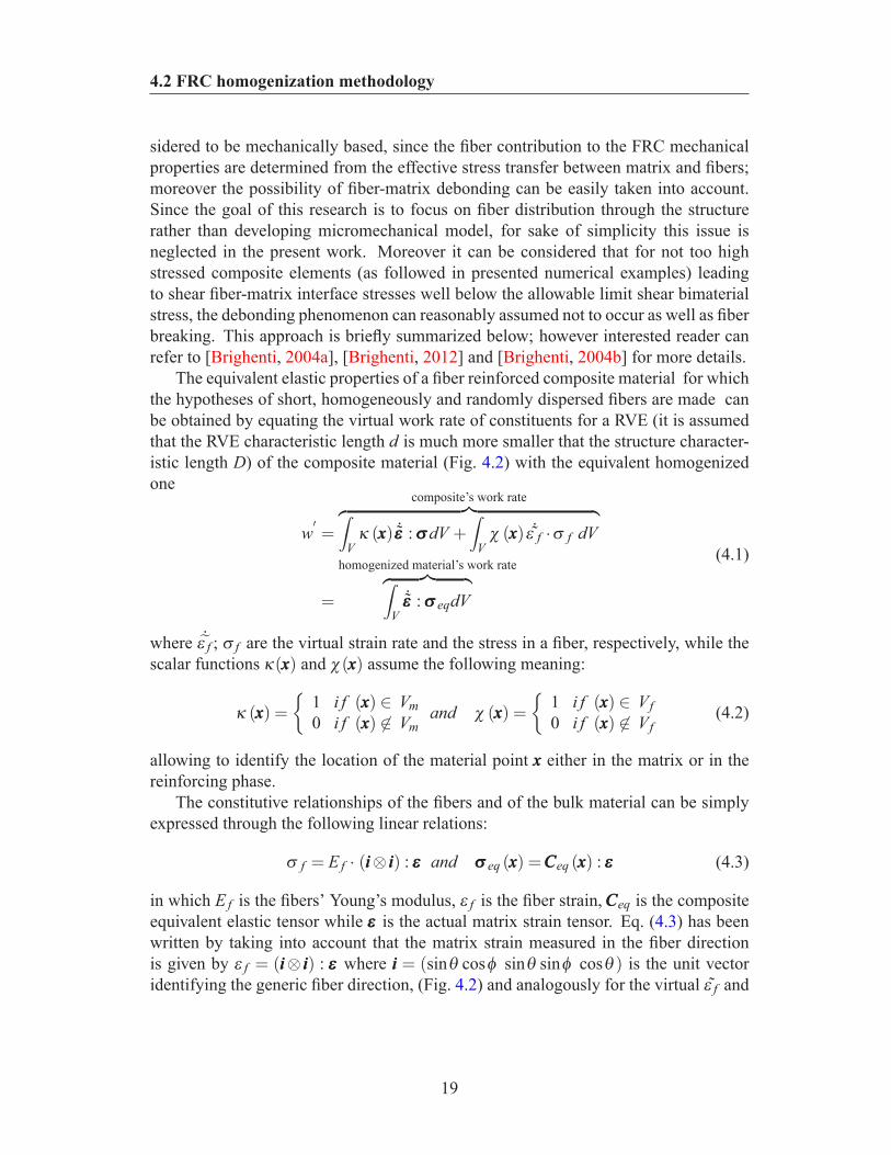
4.2 Fiber reinforced composite material: definition of the RVE (with acharacteristic length d, while the composite has a characteristic lengthD>>d) and of the fiber orientation angles φ , θ , Ref. [Brighenti, 2012] 20
4.3 Optimization algorithm . . . . . . . . . . . . . . . . . . . . . . . . . 264.4 Geometry (a) and FE mesh with control points indicated by dots (b) of
a three-point bending wall beam . . . . . . . . . . . . . . . . . . . . 274.5 Optimized fiber distribution through left half of the beam (a) current
methodology and (b) Ref. [Brighenti, 2005] . . . . . . . . . . . . . . 284.6 Optimum fiber distribution in beam considering a constant total fiber
volume equal to 10%; the maximum local fiber content is assumedequal to (a) 60% and (b) 30%; iterations results are displayed from topto bottom for each case . . . . . . . . . . . . . . . . . . . . . . . . . 29
4.7 Normalized compliance versus number of iterations for different val-ues of maximum fiber content in each element, using 264 control points 30
4.8 Schematic view of problem geometry, (a) cantilever beam (b) clampedbeam . . . . . . . . . . . . . . . . . . . . . . . . . . . . . . . . . . . 30
4.9 First modal shapes and optimum fiber distribution for a cantilever beam(a) and a clamped beam (b) . . . . . . . . . . . . . . . . . . . . . . . 31
4.10 Normalized fundamental frequency versus iterations for beam withdifferent supporting conditions . . . . . . . . . . . . . . . . . . . . . 31
4.11 (a) Schematic view of the model under uniform edges load P and (b)mesh with control points (dots) . . . . . . . . . . . . . . . . . . . . . 32
viii
LIST OF FIGURES
4.12 Optimum fiber distribution using (a) 180 control points, (b) 612 controlpoints and (c) 2244 control points . . . . . . . . . . . . . . . . . . . 33
4.13 Normalized compliance versus number of iterations for different meshsizes . . . . . . . . . . . . . . . . . . . . . . . . . . . . . . . . . . . 34
5.1 Uncertainties sources and their propagation over different length scalesand sources . . . . . . . . . . . . . . . . . . . . . . . . . . . . . . . 37
5.2 Involved scales in simulation of CNTRP [Shokrieh & Rafiee, 2010d] . 385.3 Concurrent multi-scale FE model of RVEs as micro-scale [Shokrieh &
Rafiee, 2010d] . . . . . . . . . . . . . . . . . . . . . . . . . . . . . . 385.4 RVE of composite at meso-scale [Shokrieh & Rafiee, 2010d] . . . . . 395.5 Flowchart of developed full stochastic N3M multi-scale material model
[Shokrieh & Rafiee, 2010d] . . . . . . . . . . . . . . . . . . . . . . . 405.6 Verification of the metamodel (a) mean squared error of each predicted
point (b) . . . . . . . . . . . . . . . . . . . . . . . . . . . . . . . . . 415.7 Schematic comparisons between RBDO and DDO, f stands for objec-
tive function while g1 and g2 represent design constraints . . . . . . . 425.8 Double loop RBDO flowchart . . . . . . . . . . . . . . . . . . . . . 435.9 RBDO results of a three-point bending beam with initial guess of re-
inforcement content 9% (a) and 1% (b), optimum value is 2.37% forboth (a) and (b) . . . . . . . . . . . . . . . . . . . . . . . . . . . . . 44
5.10 Definition of waviness intensity, a phenomenological concept . . . . . 455.11 Stiffness of CNTRP versus reinforcement content for different wavi-
ness intensities (a), Reliability index of the beam versus waviness (b) . 465.12 Stiffness of CNTRP versus reinforcement contents with and without
CNT agglomeration (a), Failure probability of the beam versus rein-forcement contents with and without CNT agglomeration (b). . . . . . 48
5.13 Reliability index and failure probability of the beam versus standarddeviation of load. . . . . . . . . . . . . . . . . . . . . . . . . . . . . 49
5.14 Reliability index versus FE mesh, h, parameter which is defined asthe ratio between the beam height and the number of elements in thevertical direction . . . . . . . . . . . . . . . . . . . . . . . . . . . . 49
5.15 Geometry (a), loading / boundary conditions (b), FE mesh (c) and de-formed configuration (d) of a thick cylinder under radial line load . . 50
5.16 RBDO results of a thick cylinder under radial line load for design con-straints as 1%<vol f rac<10%, 0.1<tc<0.4 (a) 1%<vol f rac<15%and 0.1<tc<0.26 (b) for both cases tc and vol f rac stand for ringthickness and reinforcement content, respectively . . . . . . . . . . . 51
ix
LIST OF FIGURES
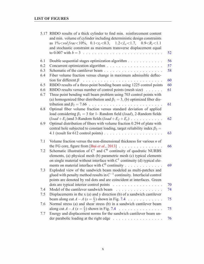
5.17 RBDO results of a thick cylinder to find min. reinforcement contentand min. volume of cylinder including deterministic design constraintsas 1%<vol f rac<10%, 0.1<tc<0.3, 1.2<Lc<1.7, 0.9<Rc<1.1and stochastic constraint as maximum transverse displacement equalto 0.007 with b = 3 . . . . . . . . . . . . . . . . . . . . . . . . . . . 52
6.1 Double sequential stages optimization algorithm . . . . . . . . . . . . 566.2 Concurrent optimization algorithm . . . . . . . . . . . . . . . . . . . 576.3 Schematic of the cantilever beam . . . . . . . . . . . . . . . . . . . . 586.4 Fiber volume fraction versus change in maximum admissible deflec-
tion for different β . . . . . . . . . . . . . . . . . . . . . . . . . . . 606.5 RBDO results of a three-point bending beam using 1225 control points 606.6 RBDO results versus number of control points (mesh size) . . . . . . 616.7 Three point bending wall beam problem using 703 control points with
(a) homogenized fiber distribution and β1 = 3, (b) optimized fiber dis-tribution and β2 = 7.66 . . . . . . . . . . . . . . . . . . . . . . . . . 61
6.8 Optimal fiber volume fraction versus standard deviation of appliedload considering β1 = 3 for 1- Random field (load), 2-Random fields(load +E f )and 3-Random fields (load +E f +Ec) . . . . . . . . . . . 62
6.9 Optimal distribution of fibers with volume fraction 0.294 of plate withcentral hole subjected to constant loading, target reliability index β2 =4.1 (result for 612 control points) . . . . . . . . . . . . . . . . . . . . 63
7.1 Volume fraction versus the non-dimensional thickness for various n ofthe FG core, figure from [Bui et al., 2013] . . . . . . . . . . . . . . . 66
7.2 Schematic illustration of C1 and C0 continuity of quadratic NURBSelements, (a) physical mesh (b) parametric mesh (c) typical elementson single material without interface with C1 continuity (d) typical ele-ments on material interface with C0 continuity . . . . . . . . . . . . . 69
7.3 Exploded view of the sandwich beam modeled as multi-patches andglued with penalty method results in C−1 continuity. Interfacial controlpoints are denoted by red dots and are coincident at interfaces. Greendots are typical interior control points . . . . . . . . . . . . . . . . . 70
7.4 Model of the cantilever sandwich beam . . . . . . . . . . . . . . . . 747.5 Displacements in the x (a) and y direction (b) of a sandwich cantilever
beam along cut A−A (x = L2 ) shown in Fig. 7.4 . . . . . . . . . . . . 75
7.6 Normal stress (a) and shear stress (b) in a sandwich cantilever beamalong cut A−A (x = L
2 ) shown in Fig. 7.4 . . . . . . . . . . . . . . . 757.7 Energy and displacement norms for the sandwich cantilever beam un-
der parabolic loading at the right edge . . . . . . . . . . . . . . . . . 76
x
LIST OF FIGURES
7.8 The first six natural frequencies of the sandwich beam with FG coreversus number of control points of the model . . . . . . . . . . . . . 78
7.9 Definition of area of interest . . . . . . . . . . . . . . . . . . . . . . 787.10 Optimal distribution of reinforcing ingredients considering area of in-
terest #1 (a), objective function versus iterations (b) . . . . . . . . . . 797.11 Shear stress profile for area #1 considering homogeneous and optimal
distribution of reinforcements, dash lines stand for face sheets whichare outside of area #1 . . . . . . . . . . . . . . . . . . . . . . . . . . 79
7.12 Optimal distribution of reinforcing ingredients considering area of in-terest #2 (a), objective function versus iterations (b) . . . . . . . . . . 80
7.13 Shear stress profile for area #2 considering homogeneous and optimaldistribution of reinforcements . . . . . . . . . . . . . . . . . . . . . . 80
7.14 Optimal distribution of reinforcing ingredients considered area of in-terest #3 (a), objective function versus iterations (b) . . . . . . . . . . 80
7.15 Shear stress profile for area #3 along a section at mid width (a) andmid length (b) of the beam considering homogeneous and optimal dis-tribution of reinforcements. In both figures, dash lines refer to zoneswhich are outside the interested area #3 . . . . . . . . . . . . . . . . 81
7.16 Optimal distribution of reinforcing ingredients considering area of in-terest #4 (a), objective function versus iterations (b) . . . . . . . . . . 82
7.17 Average of shear stress in each interfacial element along the beamlength considering area of interest #4 for pure polymer, homogeneousFRP and FRP with optimal distribution of reinforcements for (a) bot-tom interface and (b) top interface . . . . . . . . . . . . . . . . . . . 83
7.18 Nodal values of shear stress along a longitudinal sections at top in-terface (a) and bottom interface (b) in area of interest #4 comparingcharacteristics obtained by pure polymer, homogeneous FRP and FRPwith optimal distribution of reinforcements . . . . . . . . . . . . . . 84
8.1 Schematic illustration of the failure domain with two probabilistic de-sign constraints . . . . . . . . . . . . . . . . . . . . . . . . . . . . . 91
8.2 Mechanical loading and boundary conditions (a), Thermal loading andboundary conditions (b), FE discretization with red dots as controlpoints (c) . . . . . . . . . . . . . . . . . . . . . . . . . . . . . . . . 97
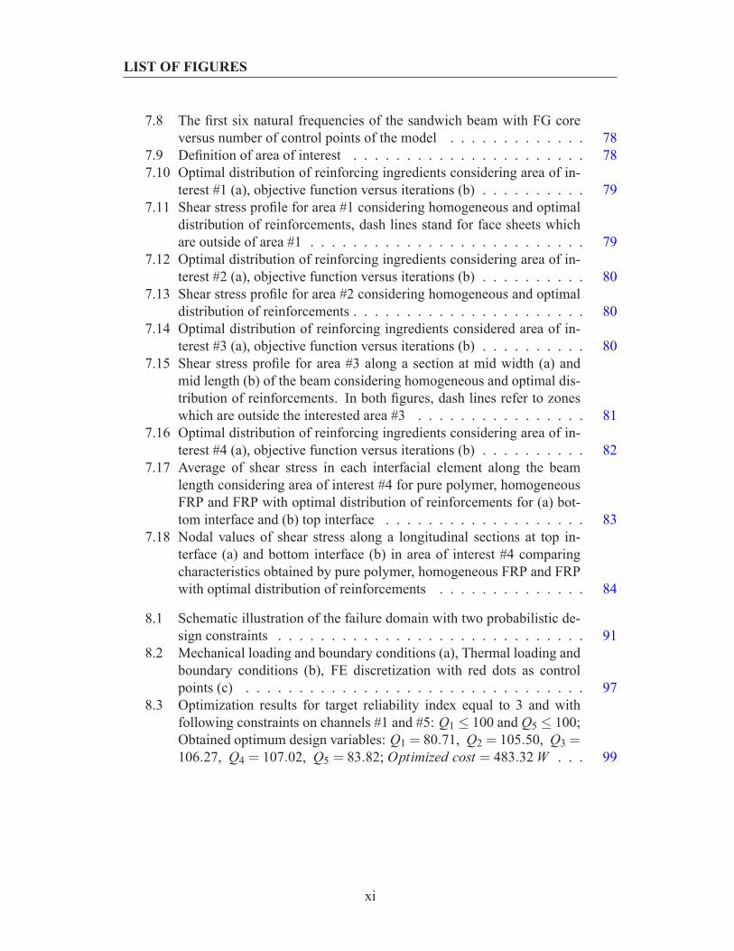
8.3 Optimization results for target reliability index equal to 3 and withfollowing constraints on channels #1 and #5: Q1 ≤ 100 and Q5 ≤ 100;Obtained optimum design variables: Q1 = 80.71, Q2 = 105.50, Q3 =106.27, Q4 = 107.02, Q5 = 83.82; Optimized cost = 483.32 W . . . 99
xi
LIST OF FIGURES
8.4 Optimization results for target reliability index equal to 3 and with fol-lowing new constraints on Channels #1, #3 and #5: Q1 ≤ 90, Q3 ≤ 90and Q5 ≤ 90; Obtained optimum design variables: Q1 = 15.81, Q2 =214.91, Q3 = 16.42, Q4 = 218.62, Q5 = 17.02; Optimized cost =482.80 W . . . . . . . . . . . . . . . . . . . . . . . . . . . . . . . . 100
8.5 Temperature (a), displacement in X-direction (b) and displacement inY-Direction (c) for CMC component with uniformly distributed C-fibers considering: Q1 = 15.81, Q2 = 214.91, Q3 = 16.42, Q4 =218.62, Q5 = 17.02 . . . . . . . . . . . . . . . . . . . . . . . . . . 100
8.6 History of the objective functions and optimal distribution of the C-fibers inside the matrix considering W1 = 1 and W2 = 0 for coupled(a) and decoupled (b) cases. Q1 = 15.81, Q2 = 214.91, Q3 = 16.42,Q4 = 218.62 and Q5 = 17.02 while the other design parameters areaccording to Table 8.1 . . . . . . . . . . . . . . . . . . . . . . . . . . 103
8.7 History of the objective functions and optimal distribution of the C-fibers inside the matrix considering W1 = 0 and W2 = 1 for coupledproblem . . . . . . . . . . . . . . . . . . . . . . . . . . . . . . . . . 103
8.8 History of the objective functions and optimal distribution of the C-fibers inside the matrix considering W1 = 1 and W2 = 0 (a) and W1 = 0and W2 = 1 (b). Both (a) and (b) are coupled problems . . . . . . . . 105
9.1 Electromechanical boundary conditions for open circuit (a) and closedcircuit (b), FE discretization with red dots representing the controlpoints (c) . . . . . . . . . . . . . . . . . . . . . . . . . . . . . . . . 120
9.2 Normalized effective piezoelectric constant e′ versus normalized beamthickness h′ . Graphs are for open circuit conditions and contain bothpiezoelectric and non-piezoelectric materials. The results for analyticsolutions are reproduced according to Eq. (9.97). . . . . . . . . . . . 121
9.3 Distribution of electric field across the beam thickness for different or-ders of basis functions. p and q are order of basis functions in directionof length and width of the beam, respectively . . . . . . . . . . . . . 122
9.4 Truncated pyramid under compression, problem setup (a) FE discretiza-tion (b) . . . . . . . . . . . . . . . . . . . . . . . . . . . . . . . . . 123
9.5 Distribution of the electric potential (left) and strain in Y direction, ε22(right) . . . . . . . . . . . . . . . . . . . . . . . . . . . . . . . . . . 124
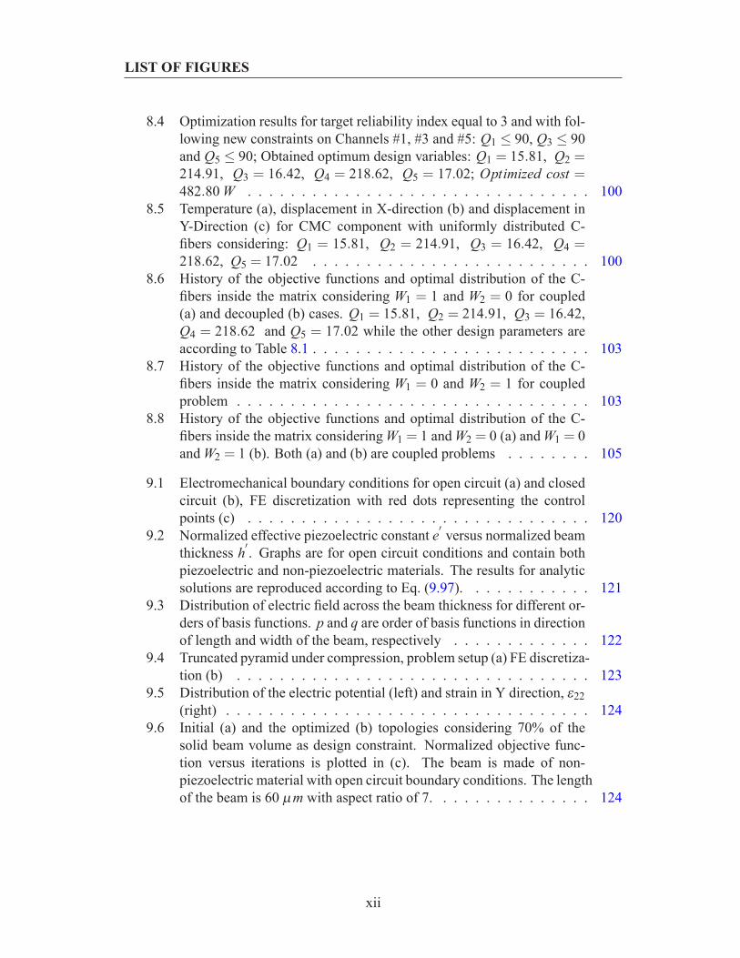
9.6 Initial (a) and the optimized (b) topologies considering 70% of thesolid beam volume as design constraint. Normalized objective func-tion versus iterations is plotted in (c). The beam is made of non-piezoelectric material with open circuit boundary conditions. The lengthof the beam is 60 µm with aspect ratio of 7. . . . . . . . . . . . . . . 124
xii
LIST OF FIGURES
9.7 cNem versus beam aspect ratio. cN
em is the ratio of the electromechanicalcoupling coefficients of the optimized structure to the solid structure.For all cases, the length of the beam is 60 µm and the optimized topol-ogy has 70% of the solid beam volume. . . . . . . . . . . . . . . . . 125
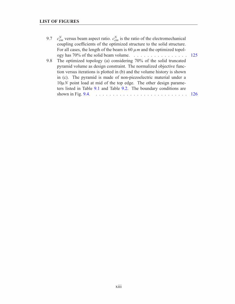
9.8 The optimized topology (a) considering 70% of the solid truncatedpyramid volume as design constraint. The normalized objective func-tion versus iterations is plotted in (b) and the volume history is shownin (c). The pyramid is made of non-piezoelectric material under a10µN point load at mid of the top edge. The other design parame-ters listed in Table 9.1 and Table 9.2. The boundary conditions areshown in Fig. 9.4. . . . . . . . . . . . . . . . . . . . . . . . . . . . 126
xiii
List of Tables
4.1 Problem definitions, wall beam under three-point bending . . . . . . . 274.2 Problem definitions, free vibration of a beam. . . . . . . . . . . . . . 304.3 Problem definitions, plate with a central circular hole under tension . . 32
5.1 Problem definitions for the beam under static loading . . . . . . . . . 445.2 Problem definitions for thick cylinder under line load . . . . . . . . . 47
6.1 Benchmark problem definitions for cantilever beam under static loading 586.2 RBDO results using analytical limit state . . . . . . . . . . . . . . . . 586.3 RBDO results using FEM limit state . . . . . . . . . . . . . . . . . . 596.4 Problem definitions of the beam under static loading . . . . . . . . . 596.5 Problem definitions, Square plate with central hole . . . . . . . . . . 62
7.1 Design data of the sandwich beam with a homogeneous elastic core . 747.2 Material properties of the sandwich beam with the FG core . . . . . . 767.3 The first six natural frequencies for a sandwich beam with FG core . . 777.4 Problem definition, cantilever sandwich beam with uniformly top load 77
8.1 Design parameters of the L-shaped component under thermomechani-cal loadings . . . . . . . . . . . . . . . . . . . . . . . . . . . . . . . 98
8.2 Summary of optimization results in Load case-1 for uniformly and op-timally distributed C-fibers with different combinations of weight factors102
8.3 New design parameters of the L-shaped component under thermome-chanical loading . . . . . . . . . . . . . . . . . . . . . . . . . . . . . 104
8.4 Summary of optimization results in Load case-2 for uniformly and op-timally distributed C-fibers with different combinations of weight factors104
9.1 The cantilever beam problem: material properties, geometry and loaddata . . . . . . . . . . . . . . . . . . . . . . . . . . . . . . . . . . . 120
9.2 The truncated pyramid problem: geometry and load data . . . . . . . 123
xiv
Chapter 1
Introduction
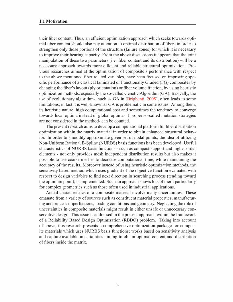
1.1 MotivationFiber Reinforced Composite (FRC) materials have been heavily investigated in the lastdecades and are widely used in advanced applications such as aerospace, structural,military and transportation industries due to their elevated mechanical properties valuesto weight (or cost) ratio. Thanks to their excellent structural qualities like high strength,fracture toughness, fatigue resistance, light weight, erosion and corrosion resistance, aparticular interest has been born not only in engineers for the use of FRCs in advancedindustrial applications, but also in researchers to develop and optimize their particularand useful characteristics.
The general behavior of a FRC depends on the characteristics of the composite con-stituents such as fiber reinforcements, resin and additives; each of these constituentshas an important role in the composite characteristics and such aspects have drivensome researchers to combine them differently for obtaining enhanced materials. Re-gardless of the roles of resins and additives which are out of the scope of this re-search, the mechanical properties of composites depend on many fiber’s variables suchas fiber’s material, volume fraction, size and mesostructure. This latter aspect whichdeals with fiber configuration, orientation, layout and dispersion is an almost openissue in the literature. Generally, increasing the fiber volume fraction in a FRC com-posite will increase its structural strength and stiffness. However the existence of apractical upper limit should be considered. Normally, composite structural elementsunder mechanical actions have some regions which are on the edge of design con-straints (e.g. the maximum allowable stress is exceeded) and can be identified as fail-ure zones. Usually these failure zones dictate the required content of the reinforcingelement in order to get a properly strengthened overall structure, fulfilling everywherethe design constraints. Considering uniform distribution of fibers through the structure,initially safe regions that already fulfill the design constraints will inevitably increase
1
1.1 Motivation
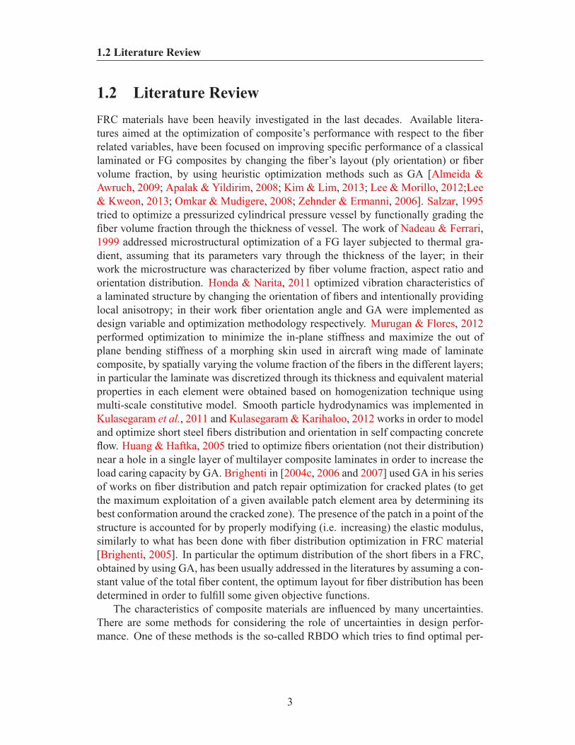
their fiber content. Thus, an efficient optimization approach which seeks towards opti-mal fiber content should also pay attention to optimal distribution of fibers in order tostrengthen only those portions of the structure (failure zones) for which it is necessaryto improve their bearing capacity. From the above discussions it appears that the jointmanipulation of these two parameters (i.e. fiber content and its distribution) will be anecessary approach towards more efficient and reliable structural optimization. Pre-vious researches aimed at the optimization of composite’s performance with respectto the above mentioned fiber related variables, have been focused on improving spe-cific performance of a classical laminated or Functionally Graded (FG) composites bychanging the fiber’s layout (ply orientation) or fiber volume fraction, by using heuristicoptimization methods, especially the so-called Genetic Algorithm (GA). Basically, theuse of evolutionary algorithms, such as GA in [Brighenti, 2005], often leads to somelimitations; in fact it is well-known as GA is problematic in some issues. Among them,its heuristic nature, high computational cost and sometimes the tendency to convergetowards local optima instead of global optima- if proper so-called mutation strategiesare not considered in the method- can be counted.
The present research aims to develop a computational platform for fiber distributionoptimization within the matrix material in order to obtain enhanced structural behav-ior. In order to smoothly approximate given set of nodal points, the idea of utilizingNon-Uniform Rational B-Spline (NURBS) basis functions has been developed. Usefulcharacteristics of NURBS basis functions - such as compact support and higher orderelements - not only provides mesh independent distribution results but also makes itpossible to use coarse meshes to decrease computational time, while maintaining theaccuracy of the results. Moreover instead of using heuristic optimization methods, thesensitivity based method which uses gradient of the objective function evaluated withrespect to design variables to find next direction in searching process (tending towardthe optimum point), is implemented. Such an approach shows lots of merit particularlyfor complex geometries such as those often used in industrial applications.
Actual characteristics of a composite material involve many uncertainties. Theseemanate from a variety of sources such as constituent material properties, manufactur-ing and process imperfections, loading conditions and geometry. Neglecting the role ofuncertainties in composite materials might result in either unsafe or unnecessary con-servative design. This issue is addressed in the present approach within the frameworkof a Reliability Based Design Optimization (RBDO) problem. Taking into accountof above, this research presents a comprehensive optimization package for compos-ite materials which uses NURBS basis functions; works based on sensitivity analysisand capture available uncertainties aiming to obtain optimal content and distributionof fibers inside the matrix.
2
1.2 Literature Review
1.2 Literature ReviewFRC materials have been heavily investigated in the last decades. Available litera-tures aimed at the optimization of composite’s performance with respect to the fiberrelated variables, have been focused on improving specific performance of a classicallaminated or FG composites by changing the fiber’s layout (ply orientation) or fibervolume fraction, by using heuristic optimization methods such as GA [Almeida &Awruch, 2009; Apalak & Yildirim, 2008; Kim & Lim, 2013; Lee & Morillo, 2012;Lee& Kweon, 2013; Omkar & Mudigere, 2008; Zehnder & Ermanni, 2006]. Salzar, 1995tried to optimize a pressurized cylindrical pressure vessel by functionally grading thefiber volume fraction through the thickness of vessel. The work of Nadeau & Ferrari,1999 addressed microstructural optimization of a FG layer subjected to thermal gra-dient, assuming that its parameters vary through the thickness of the layer; in theirwork the microstructure was characterized by fiber volume fraction, aspect ratio andorientation distribution. Honda & Narita, 2011 optimized vibration characteristics ofa laminated structure by changing the orientation of fibers and intentionally providinglocal anisotropy; in their work fiber orientation angle and GA were implemented asdesign variable and optimization methodology respectively. Murugan & Flores, 2012performed optimization to minimize the in-plane stiffness and maximize the out ofplane bending stiffness of a morphing skin used in aircraft wing made of laminatecomposite, by spatially varying the volume fraction of the fibers in the different layers;in particular the laminate was discretized through its thickness and equivalent materialproperties in each element were obtained based on homogenization technique usingmulti-scale constitutive model. Smooth particle hydrodynamics was implemented inKulasegaram et al., 2011 and Kulasegaram & Karihaloo, 2012 works in order to modeland optimize short steel fibers distribution and orientation in self compacting concreteflow. Huang & Haftka, 2005 tried to optimize fibers orientation (not their distribution)near a hole in a single layer of multilayer composite laminates in order to increase theload caring capacity by GA. Brighenti in [2004c, 2006 and 2007] used GA in his seriesof works on fiber distribution and patch repair optimization for cracked plates (to getthe maximum exploitation of a given available patch element area by determining itsbest conformation around the cracked zone). The presence of the patch in a point of thestructure is accounted for by properly modifying (i.e. increasing) the elastic modulus,similarly to what has been done with fiber distribution optimization in FRC material[Brighenti, 2005]. In particular the optimum distribution of the short fibers in a FRC,obtained by using GA, has been usually addressed in the literatures by assuming a con-stant value of the total fiber content, the optimum layout for fiber distribution has beendetermined in order to fulfill some given objective functions.
The characteristics of composite materials are influenced by many uncertainties.There are some methods for considering the role of uncertainties in design perfor-mance. One of these methods is the so-called RBDO which tries to find optimal per-
3
1.3 Objectives of the dissertation
formance considering some probabilistic design constraints. Motivated by capabilitiesof RBDO in uncertainty quantification, some researchers have implemented it in thedesign of composite structures. Though there are some exceptions, most of these re-searches are related to composite laminates. However, to the knowledge of the author,the solid FRC structures are not thoroughly explored. Thanedar & Chamis, 1995 de-veloped a procedure for the tailoring of layered composite laminates subjected to prob-abilistic constraints and loads. The work of Jiang et al., 2008 suggested a methodologyto optimize the plies orientations of a composite laminated plate having uncertain mate-rial properties. Gomes & Awruch, 2011 addressed the problem of composite laminateoptimization by using GA and Artificial Neural Networks (ANN); while Antonio &Hoffbauer, 2009 presented reliability based robust design optimization methodology.Noh & Kang., 2013 have implemented RBDO methodology for purpose of optimizingvolume fraction in a FG laminate composite.
Uncertainty propagation in nanocomposite structures remains an unsolved issue.Rouhi & Rais-Rohani, 2013 measured the failure probability of a nanocomposite cylin-der under buckling, accounting for uncertain design conditions. However, they usedmicromechanical equations at the nano-scale by simply replacing the lattice structureof a Carbon Nano Tube (CNT) with a solid fiber (which can lead to inappropriateresults Shokrieh & Rafiee, 2010c). Moreover, they disregard several important CNTparameters such as the CNT length, diameter, agglomeration and dispersion withoutany sensitivity evaluation. Furthermore, modeling errors including discretization- andapproximation errors have not been addressed in detail.
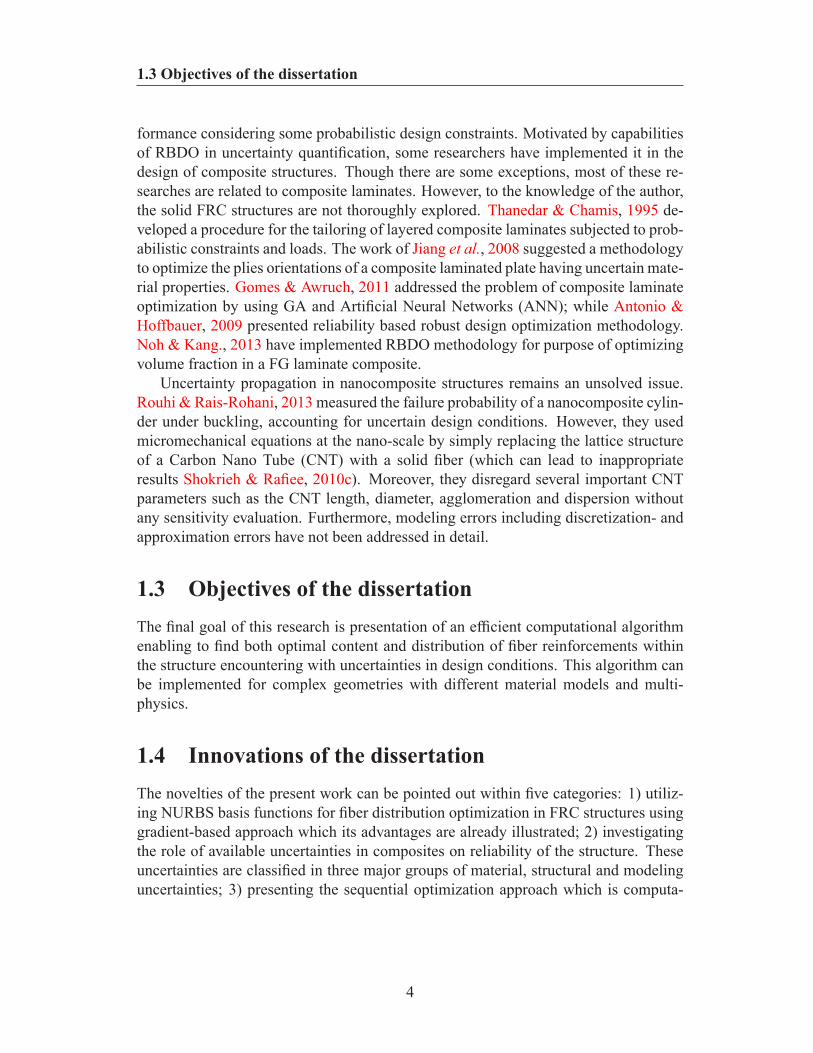
1.3 Objectives of the dissertationThe final goal of this research is presentation of an efficient computational algorithmenabling to find both optimal content and distribution of fiber reinforcements withinthe structure encountering with uncertainties in design conditions. This algorithm canbe implemented for complex geometries with different material models and multi-physics.
1.4 Innovations of the dissertationThe novelties of the present work can be pointed out within five categories: 1) utiliz-ing NURBS basis functions for fiber distribution optimization in FRC structures usinggradient-based approach which its advantages are already illustrated; 2) investigatingthe role of available uncertainties in composites on reliability of the structure. Theseuncertainties are classified in three major groups of material, structural and modelinguncertainties; 3) presenting the sequential optimization approach which is computa-
4
1.5 Outline
tionally efficient and links RBDO and fiber distribution optimization; 4) implementingthe methodology in innovative applications including interfacial shear stress optimiza-tion in sandwich beam and optimization of internal cooling channels in Ceramic MatrixComposite (CMC); 5) adopting the computational framework for topology optimiza-tion of piezoelectric / flexoelectric materials.
1.5 OutlineIn the previous sections, the topic, objective, innovations, literature review and method-ology of the thesis are introduced. The remainder of this dissertation is organized asfollows:
Chapter 2 contains fundamental formulations of Isogeometric Analysis (IGA) andNURBS basis functions which are used in this dissertation.
Chapter 3 deals with structural reliability concept. The notions of reliability assess-ment, RBDO and First Order Reliability Method (FORM) which are frequently usedin this dissertation are introduced.
Chapter 4 deals with the optimization of short fibers distribution in continuum struc-tures made of FRC by adopting an efficient gradient based optimization approach.NURBS basis functions have been implemented to define continuous and smooth meshindependent fiber distribution function as well as domain discretization. Some numer-ical examples related to the structural response under static loading as well as the freevibration behavior are conducted to demonstrate the capabilities of the model.
Chapter 5 focuses on the uncertainties propagation and their effects on reliability ofpolymeric nanocomposite (PNC) continuum structures, in the framework of the com-bined geometry and material optimization. Presented model considers material, struc-tural and modeling uncertainties. The material model covers uncertainties at differentlength scales (from nano-, micro-, meso- to macro-scale) via a stochastic approach. Itconsiders the length, waviness, agglomeration, orientation and dispersion (all as ran-dom variables) of CNTs within the polymer matrix. To increase the computationalefficiency, the expensive-to-evaluate stochastic multi-scale material model has beensurrogated by a kriging metamodel. This metamodel-based probabilistic optimizationhas been adopted in order to find the optimum value of the CNT content as well as theoptimum geometry of the component as the objective function while the implicit finiteelement based design constraint is approximated by the first order reliability method.Illustrative examples are provided to demonstrate the effectiveness and applicability ofthe approach.
5

1.5 Outline
Chapter 6 presents double stage sequential optimization algorithm for finding the opti-mal fiber content and its distribution in solid composites, considering uncertain designparameters. In the first stage, the optimal amount of fiber in a FRC structure withuniformly distributed fibers is conducted in the framework of a RBDO problem. Inthe second stage, the fiber distribution optimization having the aim to more increasein structural reliability is performed by defining a fiber distribution function through aNURBS surface. Some case studies are performed to demonstrate the capabilities ofthe model.
Chapter 7 contains the first application of the methodology in sandwich beams withpolymeric core to decrease interfacial stresses by presenting the optimal distributionof reinforcing ingredients in the polymeric matrix. This application aims at the localstress minimization within any arbitrary zone of the design domain. The core and facesheets are modeled as multi-patches and compatibility in the displacement field is en-forced by the penalty method. An adjoint sensitivity method is devised to minimize theobjective function within areas of interest defined over arbitrary regions in the designdomain. The method is verified by several examples.
Chapter 8 contains the second application of the methodology for optimization of theinternal cooling channels in Ceramic Matrix Composite (CMC) under thermal andmechanical loadings. The algorithm finds the optimal cooling capacity of all channels(which directly minimizes the amount of coolant needed). In the first step, availableuncertainties in the constituent material properties, the applied mechanical load, theheat flux and the heat convection coefficient are considered. Using RBDO approach,the probabilistic constraints ensure the failure due to excessive temperature and deflec-tion will not happen. The deterministic constraints restrict the capacity of any arbi-trary cooling channel between two extreme limits. A series system reliability conceptis adopted as a union of mechanical and thermal failure subsets. Having the resultsof the first step for CMC with uniformly distributed carbon (C-) fibers, the algorithmpresents the optimal layout for distribution of the C-fibers inside the ceramic matrixin order to enhance the target reliability of the component. A sequential approach andB-spline finite elements have overcome the cumbersome computational burden. Nu-merical examples are presented.
Chapter 9 presents a design methodology based on a combination of IGA, level setand point wise density mapping techniques for topology optimization of piezoelec-tric / flexoelectric materials. The fourth order partial differential equations (PDEs) offlexoelectricity, which require at least C1 continuous approximations, are discretizedusing NURBS. The point wise density mapping technique with consistent derivativesis directly used in the weak form of the governing equations. The boundary of the
6

1.5 Outline
design domain is implicitly represented by a level set function. The accuracy of theIGA model is confirmed through numerical examples including a cantilever beam un-der a point load and a truncated pyramid under compression with different electricalboundary conditions. Numerical examples demonstrate the usefulness of the method.
Chapter 10 summarizes the works and outlines the main contributions. Finally, somerecommendations for future work are suggested.
7
Chapter 2
Fundamentals of NURBS
2.1 An introduction to Isogeometric AnalysisThe main tool that is used by Computer Aided Design (CAD) for representation of thecomplex geometries is the Non-Uniform Rational B-spline (NURBS). Using NURBS,certain geometries including conic and circular sections, can be represented exactly.That is while polynomial shape functions are able to just approximate the geometries.The main idea behind the seminal work of Hughes et al., 2005 was using NURBSnot only for describing the geometry but also to construct finite approximations foranalysis. The phrase ’Isogeometric Analysis’ (IGA) was firstly used by Hughes et al.to unify CAD and Computer Aided Engineering (CAE). In the following fundamentalformulations of IGA which are used in this dissertation are introduced. Readers arereferred to [Cottrell et al., 2009] to know more about IGA.
2.2 Knot vectorThere are two different spaces in IGA named physical space and parameter space. Eachelement in the physical space is the image of a corresponding element in the parameterspace, but the mapping itself is global to the whole patch, rather than to the elementsthemselves. The parameter space is discretized by knot vectors. A knot vector inone dimension is a non-decreasing set of coordinates in the parameter space, writtenΞΞΞ=
ξ1,ξ2, ...,ξn+p+1
, where ξi ∈ R is the ith knot, i is the knot index, i= 1,2, ...,n+
p+1, p is the polynomial order and n is the number of basis functions used to constructthe B-spline curve. Element boundaries in the physical space are simply the imagesof knot lines under the B-spline mapping (See Fig. 2.1). Equally spaced knots in theparameter space provide uniform knot vectors, otherwise they are non-uniform. Aknot vector is said to be open if its first and last knot values appear p+1 times. Openknot vectors are the standard in the CAD literature. In one dimension, basis functions
8
2.3 NURBS functions and surfaces
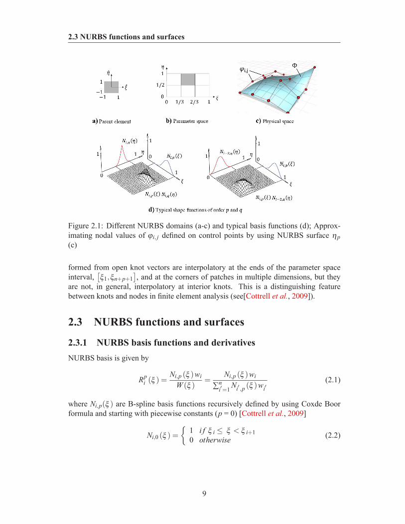
Figure 2.1: Different NURBS domains (a-c) and typical basis functions (d); Approx-imating nodal values of ϕi, j defined on control points by using NURBS surface ηp(c)
formed from open knot vectors are interpolatory at the ends of the parameter spaceinterval,
[ξ1,ξn+p+1
], and at the corners of patches in multiple dimensions, but they
are not, in general, interpolatory at interior knots. This is a distinguishing featurebetween knots and nodes in finite element analysis (see[Cottrell et al., 2009]).
2.3 NURBS functions and surfaces
2.3.1 NURBS basis functions and derivativesNURBS basis is given by
Rpi (ξ ) =
Ni,p (ξ )wiW (ξ )
=Ni,p (ξ )wi
∑ni′=1 Ni′ ,p (ξ )wi′
(2.1)
where Ni,p(ξ ) are B-spline basis functions recursively defined by using Coxde Boorformula and starting with piecewise constants (p = 0) [Cottrell et al., 2009]
Ni,0 (ξ ) =
1 i f ξ i ≤ ξ < ξ i+10 otherwise (2.2)
9
2.3 NURBS functions and surfaces
while for p = 1, 2, 3, . . .
Ni,p (ξ ) =ξ −ξ i
ξ i+p −ξ iNi,p−1 (ξ )+
ξ i+p+1 −ξξ i+p+1 −ξ i+1
Ni+1,p−1 (ξ ) (2.3)
wi is also referred to as the ith weight while W (ξ ) is weighting function defined asfollows:
W (ξ ) =n
∑i=1
Ni,p (ξ )wi (2.4)
Simply applying the quotient rule to Eq. (2.1) yields:
ddξ
Rpi (ξ ) = wi
W (ξ )N ′
i,p (ξ )−W ′(ξ )Ni,p(ξ )
(W (ξ ))2 (2.5)
whereN
′
i,p (ξ ) =p
ξ i+p −ξ iNi,p−1 (ξ )−
pξ i+p+1 −ξ i+1
Ni+1,p−1 (ξ ) (2.6)
andW
′(ξ ) =
n
∑i=1
N′
i,p (ξ )wi (2.7)
Among NURBS basis functions characteristics, the most important ones are partitionof unity property, compact support of each basis function and non-negative values. Itcan be also noted that if the weights are all equal, then Rp
i (ξ ) = Ni,p(ξ ); so, B-splineis the special case of NURBS. Details related to higher order derivatives formulationscan be found in [Cottrell et al., 2009].
2.3.2 NURBS curves and surfacesA NURBS curve is defined as:
C (ξ ) =n
∑i=1
Rpi (ξ )Bi (2.8)
where Bi ∈ Rd are control points and i = 1,2, ...,n, number of control points. Similarly,for definition of a NURBS surface, two knot vectors EEE =
ξ1,ξ2, ...,ξn+p+1
and HHH =
η1,η2, ...,ηm+q+1
(one for each direction) as well as a control net Bi, j are required.A NURBS surface is defined as:
S (ξ ,η) =n
∑i=1
m
∑j=1
Rp,qi, j (ξ ,η)Bi, j (2.9)
10

2.3 NURBS functions and surfaces
where Rp,qi, j (ξ ,η) is defined according to the following Eq. (2.10), while Ni,p(ξ ) and
M j,q(η) are univariate B-spline basis functions of order p and q corresponding to knotvector EEE and HHH, respectively.
Rp,qi, j (ξ ,η) =
Ni,p (ξ )M j,q (η)wi, j
∑ni′=1∑
mj′=1 Ni′ ,p (ξ )M j′ ,q(η)wi′ , j′
(2.10)
11
Chapter 3
Structural reliability
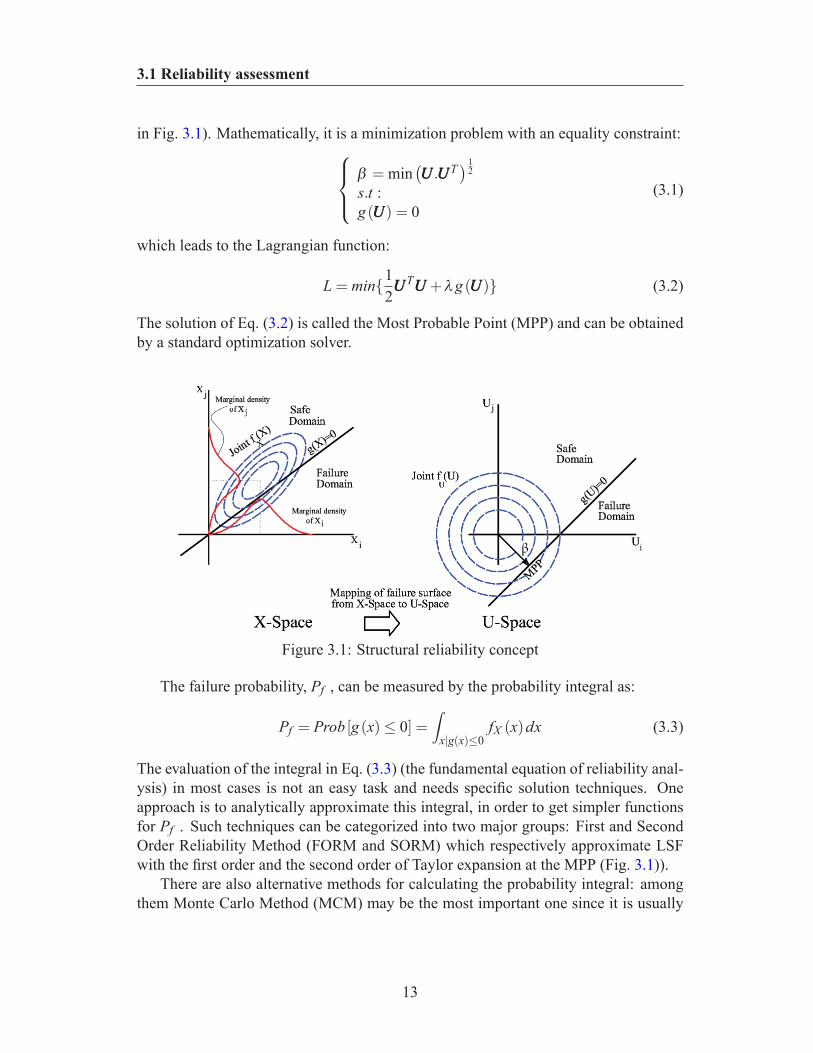
3.1 Reliability assessmentThe fundamentals of structural reliability are briefly presented below however, inter-ested readers can refer to [Ditlevsen & Madsen, 1996] and references therein for moredetails. The structural reliability concept can be simply described by the example of asteel rod with constant cross sectional area under uniaxial tension (see Fig. 3.1). In thedeterministic case, if the applied load (L) is less than rod strength (R), failure will notoccur and the rod will be safe and the conventional safety factor index (S.F = R
L ) is usedto quantify the system level of confidence. In probabilistic case, (L) and (R) are notfixed values but instead they are random variables containing uncertainties. In this caseX(L) and X(R)are non-negative independent random variables with Probability Den-sity Functions (PDF) fL(xL) and fR(xR), respectively. In essence, for a vector of ran-dom variables X = x1, ...,xn
T , the PDF can be calculated by fX(x) = ddx
FX(x), whereFX(x) is the so called Cumulative Distribution Function (CDF) and relates the probabil-ity of a random event to a prescribed deterministic value x, (i.e. FX(x) = Prob X<x).
In considering the rod example, the boundary between safe (i.e. xR>xL) and failure(i.e. xR<xL) regions can be defined by g(x) = xR − xL which is called Limit StateFunction (LSF). Thus, g(x)≤ 0 denotes a subset of the space, where failure occurs.
The concept of Reliability Index (β ) which has been proposed by Hasofer & Lind,1974 requires standard normal non-correlated variables; so the transformations fromcorrelated non-Gaussian variables X to uncorrelated Gaussian variables U (with zeromeans and unit standard deviations) is needed. According to this definition of β , thedesign point is chosen such as to maximize the PDF within the failure domain. Ge-ometrically, it corresponds to the point in failure domain having the shortest distancefrom the origin of reduced variables to the limit state surface (i.e. g(U) = 0), as shown
12
3.1 Reliability assessment
in Fig. 3.1). Mathematically, it is a minimization problem with an equality constraint:
β = min(UUU .UUUT) 1
2
s.t :g(UUU) = 0
(3.1)
which leads to the Lagrangian function:
L = min12
UUUTUUU +λg(UUU) (3.2)
The solution of Eq. (3.2) is called the Most Probable Point (MPP) and can be obtainedby a standard optimization solver.
Figure 3.1: Structural reliability concept
The failure probability, Pf , can be measured by the probability integral as:
Pf = Prob [g(x)≤ 0] =∫
x|g(x)≤0fX (x)dx (3.3)
The evaluation of the integral in Eq. (3.3) (the fundamental equation of reliability anal-ysis) in most cases is not an easy task and needs specific solution techniques. Oneapproach is to analytically approximate this integral, in order to get simpler functionsfor Pf . Such techniques can be categorized into two major groups: First and SecondOrder Reliability Method (FORM and SORM) which respectively approximate LSFwith the first order and the second order of Taylor expansion at the MPP (Fig. 3.1)).
There are also alternative methods for calculating the probability integral: amongthem Monte Carlo Method (MCM) may be the most important one since it is usually
13
3.1 Reliability assessment
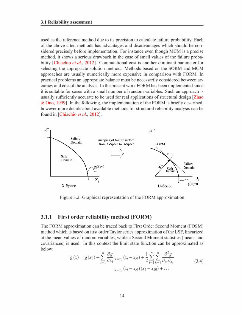
used as the reference method due to its precision to calculate failure probability. Eachof the above cited methods has advantages and disadvantages which should be con-sidered precisely before implementation. For instance even though MCM is a precisemethod, it shows a serious drawback in the case of small values of the failure proba-bility [Chiachio et al., 2012]. Computational cost is another dominant parameter forselecting the appropriate solution method. Methods based on the SORM and MCMapproaches are usually numerically more expensive in comparison with FORM. Inpractical problems an appropriate balance must be necessarily considered between ac-curacy and cost of the analysis. In the present work FORM has been implemented sinceit is suitable for cases with a small number of random variables. Such an approach isusually sufficiently accurate to be used for real applications of structural design [Zhao& Ono, 1999]. In the following, the implementation of the FORM is briefly described,however more details about available methods for structural reliability analysis can befound in [Chiachio et al., 2012].
Figure 3.2: Graphical representation of the FORM approximation
3.1.1 First order reliability method (FORM)The FORM approximation can be traced back to First Order Second Moment (FOSM)method which is based on first order Taylor series approximation of the LSF, linearizedat the mean values of random variables, while a Second Moment statistics (means andcovariances) is used. In this context the limit state function can be approximated asbelow:
g(x) = g(x0)+n
∑i=1
∂g∂xi
|x=x0(xi − xi0)+
12
n
∑i=1
n
∑k=1
∂ 2g∂ xi∂ xk
|x=x0(xi − xi0)(xk − xk0)+ . . .
(3.4)
14
3.1 Reliability assessment
Terminating the series after the linear terms yields:
E[Z] = E [g(XXX)] = g(x0)+n
∑i=1
∂g∂xiE [xi − xi0] (3.5)
where E stands for expected value (or ensemble average) of a random quantity g(XXX)and can be defined in terms of the probability density function of x as:
E [g(XXX)] =∫ +∞
−∞g(x) fX (x)dx (3.6)
If the mean value vector X is chosen as the starting expansion point x0 for the Taylorseries, then E[Z] = g(x0) and the variance becomes:
σ2Z = E
[(Z − Z)2
]= E
[(g(XXX)−g
(XXX))
2]= E
(
n
∑i=1
∂g∂X i
(Xi − Xi)
)2
=n
∑i=1
n
∑k=1
∂g∂xi
∂g∂xk
E[(Xi − Xi)(Xk − Xk)]
(3.7)
finally the distribution function Fz(z) is approximated by a normal distribution:
Fz (Z) =Φ(
z− ZσZ
)(3.8)
then we obtain the approximate result:
Pf = Fz (0) =Φ(−
ZσZ
)(3.9)
the reliability R can finally be expressed as:
R =Φ(β ) (3.10)
where β = zσz
and the probability of failure consequently becomes expressed as:
Pf = 1−R = 1−Φ(β ) =Φ(−β ) (3.11)
3.1.2 RBDOIn its basic form the problem of RBDO can be expressed as below:
Minimize C (θθθ) s.t.∣∣∣∣
f1 (θθθ) , . . . , fq−1 (θθθ)≤ 0fq (XXX ,θθθ) = β t −β (XXX ,θθθ)≤ 0 (3.12)
15

3.1 Reliability assessment
where θθθ is the vector of the design variables, C(θθθ) is the cost or objective function,f1(θθθ), ..., fq1(θθθ) is a vector of q−1 deterministic constraints over the design variablesθθθ , fq(XXX ,θθθ) is the reliability constraint enforcing the respect of LSF and consideringthe uncertainty to which some of the model parameters XXX are subjected to. βt is thetarget safety index. In this dissertation, to solve Eq. (3.12), the open source softwareFERUM 4.1 ([Bourinet, 2010]) has been implemented and linked to FE code whichevaluates the LSF.
16
Chapter 4
Optimization of fiber distribution infiber reinforced composite
4.1 IntroductionThe mechanical properties of composites depend on many fiber’s variables such asfibers material, volume fraction, size and mesostructure. This latter aspect deals withfiber configuration, orientation, layout and dispersion. As reviewed in Chapter 1, avail-able literatures aimed at the optimization of composite’s performance with respectto the above mentioned fiber related variables, have been focused on improving spe-cific performance of a classical laminated or Functionally Graded (FG) composites bychanging the fiber’s layout (ply orientation) or fiber volume fraction, by using heuristicoptimization methods, especially the so-called Genetic Algorithm (GA).
Computational cost is a very important aspect in optimization problem, particu-larly in industrial applications. Basically, the use of evolutionary algorithms, such asGA, often leads to some limitations; in fact it is well-known as GA is problematic insome issues. Among them, its heuristic nature, high computational cost and sometimesthe tendency to converge towards local optima instead of global optima - if proper so-called mutation strategies are not considered in the method - can be counted. In con-trary with GA, gradient based methods which use gradient of the objective functionevaluated with respect to design variables to find next direction in searching process(tending toward the optimum point), shows lots of merit particularly for complex ge-ometries such as those often used in industrial applications.
There are also some limitations in using FE mapping of the fiber content [Brighenti,2005] due to the element wise poor representation of the fiber layout: the first one isthe possibility of mesh dependency for the results, since the final fibers arrangementresulting from the optimization is commonly determined based on fiber content ofeach finite element. Secondly, it could be easily understood that in order to have good
17
4.2 FRC homogenization methodology
layout representation, fine mesh and consequently costly computation should be done;moreover further post processing technique such as filtering or smoothing becomesnecessary when this method is implemented. Thirdly, it must be also considered that,before economical and technological evaluations are performed, to fabricate element-wise variation of fiber content in a discretized continuum structure is still a dauntingstep with present available technologies. Fig. 4.1 schematically shows such limitationsinvolved in FE mapping representation.
Figure 4.1: Schematic illustration of mesh dependency in element-based representationof fiber volume fraction: a) Coarse mesh b) Fine mesh
Instead of using element-based fiber volume fraction description, as has been al-ready done in other researches, the idea of utilizing quadratic NURBS basis functionsin order to smoothly and continuously approximate given set of nodal points are devel-oped. Useful characteristics of NURBS basis functions such as compact support andhigher order elements not only provides mesh independent distribution results but alsomakes it possible to use coarse meshes to decrease computational time, while maintain-ing the accuracy of the results. The presented novel computational approach combinesNURBS based and gradient based optimization methodologies to get an efficient op-timization algorithm, which has been verified to be enough accurate, computationallyfast and convenient for real industrial applications.
4.2 FRC homogenization methodologyBasically the aim of homogenization techniques is to determine equivalent materialcharacteristics in a Representative Volume Element (RVE) of composite material. Thereare some classical approaches in order to model the material properties of composites;among which the rule of mixture, Hashin-Shtrikman type bounds [Hashin, 1962 andHashin & Shtrikman, 1963], Variational Bounding Techniques [Paul, 1960], Self Con-sistency Method [Hill, 1965] and Mori-Tanaka Method [Mori & Tanaka, 1973] can bementioned. The homogenization approach used in this chapter is a simplified versionof recently developed mechanical model [Brighenti, 2004a], to get the FRC consti-tutive behavior based on the shear stress distribution along the fiber-matrix interfaceduring the loading process. The adopted model for fiber homogenization can be con-
18
4.2 FRC homogenization methodology
sidered to be mechanically based, since the fiber contribution to the FRC mechanicalproperties are determined from the effective stress transfer between matrix and fibers;moreover the possibility of fiber-matrix debonding can be easily taken into account.Since the goal of this research is to focus on fiber distribution through the structurerather than developing micromechanical model, for sake of simplicity this issue isneglected in the present work. Moreover it can be considered that for not too highstressed composite elements (as followed in presented numerical examples) leadingto shear fiber-matrix interface stresses well below the allowable limit shear bimaterialstress, the debonding phenomenon can reasonably assumed not to occur as well as fiberbreaking. This approach is briefly summarized below; however interested reader canrefer to [Brighenti, 2004a], [Brighenti, 2012] and [Brighenti, 2004b] for more details.
The equivalent elastic properties of a fiber reinforced composite material for whichthe hypotheses of short, homogeneously and randomly dispersed fibers are made canbe obtained by equating the virtual work rate of constituents for a RVE (it is assumedthat the RVE characteristic length d is much more smaller that the structure character-istic length D) of the composite material (Fig. 4.2) with the equivalent homogenizedone
w′=
composite’s work rate︷ ︸︸ ︷∫
Vκ (xxx) ˙εεε :σσσdV +
∫
Vχ (xxx) ˙ε f ·σ f dV
=
homogenized material’s work rate︷ ︸︸ ︷∫
V˙εεε :σσσ eqdV
(4.1)
where ˙ε f ; σ f are the virtual strain rate and the stress in a fiber, respectively, while thescalar functions κ(xxx) and χ(xxx) assume the following meaning:
κ (xxx) =
1 i f (xxx) ∈ Vm0 i f (xxx) 6∈ Vm
and χ (xxx) =
1 i f (xxx) ∈ V f0 i f (xxx) 6∈ V f
(4.2)
allowing to identify the location of the material point xxx either in the matrix or in thereinforcing phase.
The constitutive relationships of the fibers and of the bulk material can be simplyexpressed through the following linear relations:
σ f = E f · (iii⊗ iii) : εεε and σσσ eq (xxx) =CCCeq (xxx) : εεε (4.3)
in which E f is the fibers’ Young’s modulus, ε f is the fiber strain, CCCeq is the compositeequivalent elastic tensor while εεε is the actual matrix strain tensor. Eq. (4.3) has beenwritten by taking into account that the matrix strain measured in the fiber directionis given by ε f = (iii⊗ iii) : εεε where iii = (sinθ cosφ sinθ sinφ cosθ) is the unit vectoridentifying the generic fiber direction, (Fig. 4.2) and analogously for the virtual ε f and
19

4.2 FRC homogenization methodology
the virtual strain rate,
ε f = (iii⊗ iii) : εεε and ˙ε f = (iii⊗ iii) : ˙εεε (4.4)
By substituting the above expressions in the virtual work rate equality (Eq. (4.1)) onecan finally identify the composite equivalent elastic tensor
CCCeq (xxx) =1V
∫
Vκ (xxx)CCCm +χ (xxx)E f [QQQ⊗QQQ]dV
= µCCCm +η pE f
∫
VQQQ⊗QQQ dV
(4.5)
where the second-order tensor QQQ = (iii⊗iii) has been introduced and the matrix and fibervolume fractions µ = 1
V∫
V κ(xxx)dV = VmV and ηp =
1V∫
V χ(xxx)dV =V fV have been used.
It can be easily deduced as the equivalent material is macroscopically homogeneous atleast at the scale of the RVE with volume V - i.e. the equivalent elastic tensor CCCeq(xxx)does not depend on the position vector, i.e. CCCeq(xxx) =CCCeq.
The calculation of the equivalent elastic tensor CCCeq through Eq. (4.5), requires toevaluate the integral in Eq. (4.5) over a sufficiently large volume, representative of themacroscopic characteristics of the composite. The above integral can be suitably as-sessed on a hemisphere volume which allows considering all possible fiber orientationsin the composite
Figure 4.2: Fiber reinforced composite material: definition of the RVE (with a char-acteristic length d, while the composite has a characteristic length D>>d) and of thefiber orientation angles φ , θ , Ref. [Brighenti, 2012]
20
4.3 Definition of the optimization problem
1Vhem
∫
VhemQQQ⊗QQQdV =
∫ R
0
∫ 2π
0
∫ π/2
0(QQQ⊗QQQ)r dφ r sinθdθ dr
=R3
31
2πR33
∫ 2π
0
∫ π/2
0(QQQ⊗QQQ)dφ sinθ dθ
=1
2π
∫ 2π
0
∫ π/2
0(QQQ⊗QQQ)dφ sinθ dθ
(4.6)
In the above expression the case of fibers randomly distributed in the 3D space has beenconsidered, but the generic case of preferentially oriented fibers can be also treated ina similar way [Brighenti & Scorza, 2012].
4.3 Definition of the optimization problemLots of structural characteristics or responses can be adopted as optimization objec-tives. As representative examples one can mention weight, stiffness, natural frequen-cies or a combination of them. Optimization aimed at obtaining structures with mini-mum strain energy (minimum structural compliance), which alternatively means max-imum structural stiffness, is the most common approach in this field. Nevertheless,though combination of elastic compliance with structural volume or weight constraintsis comprehensive for static problems, obtained designs are not essentially optimumconsidering dynamic behavior of the structure. One important example is representedby vibrating structures to be designed in such a manner to avoid resonance for ex-ternal excitation loads varying with a given frequency. This goal is usually obtainedby maximizing the fundamental eigenfrequency or the gap between two consecutiveeigenfrequencies of the structure [Du & Olhoff, 2007].
In the context of this chapter just the optimization of fiber distribution throughthe structure will be addressed. Definition of single objective function either for purestatic loading or free vibration is considered. Extension of this methodology into multi-objective problems, which deals with systematic and concurrent solution of a collectionof objective functions, will be straight forward in formulation. Typical multi-objectiveoptimization problem consists of a weighted sum of all objective functions combinedto a form of single function. Final solution of this function is totally dependent onthe allocated weights. On the other hand from the technological point of view, engi-neers need to know a specific volume fraction for design and manufacturing of a FRCproduct. Generally there is no single global solution for multi-objective optimizationproblems and selection of a set of points as a final solution among thousands of pos-sible solutions requires to develop a comprehensive selection criteria which is behindthe scope of this chapter. To review the multi-objective optimization methods in engi-neering, interested readers can refer to [Marler & Arora, 2004].
21
4.3 Definition of the optimization problem
4.3.1 Objective function and optimization formulation for staticproblems
Strain energy can be considered as the work done by internal forces through the de-formation of the body. This energy is considered as the objective function of the opti-mization problem. For the problem with m-load cases we have
U =m
∑i=1
λ iU i λ i > 0 (4.7)
where U and U i are the total strain energy and elastic strain energy for the ith loadcase respectively; while λi is the weight associated to the strain energy which has beenconsidered equal to unity unless otherwise specified.The terms U i can be defined as
U i = [nel
∑e=1
12
∫
VεεεT
e CCCeq εεεedV ]
i
(4.8)
in the above equation εεεe is the strain vector associated with element e and CCCeq is thehomogenized elastic tensor of the composite at each point according to Eq. (4.5), whilenel is the number of elements in the structural component being analyzed.
Nodal fiber volume fraction ϕi, j (the subscripts i and j belong to counterpart con-trol point, Bi, j) on control points are defined as design variables and fiber distributionis approximated by using NURBS surface (see Eq. (2.10) and Fig. 2.1(c)) based on for-mulation provided in Chapter 2. Every point on parametric mesh space of the designdomain will be mapped to geometrical space having two distinguished identifications,i.e. geometrical coordinates and fiber volume fraction value. Intrinsically, even usingcoarse meshes, distribution function described through a NURBS surface is smoothenough to have clear representation with no need to any further image processing tech-nique.
Fiber distribution function ηp(x,y)- which indicates the fiber amount at every de-sign point and will be used for obtaining homogenized mass and stiffness of finiteelements- is defined according to the following relationship
η p(x,y) =n
∑i=1
m
∑j=1
Rp,qi, j (ξ ,η)ϕ i, j (4.9)
Once the fiber volume fraction at each point is available, by substitution in Eq. (4.5),we can define the equivalent mechanical characteristics of the domain through thefollowing equations
CCCeq(x,y) =(1−η p
)CCCm +η pE f
∫
VQQQ⊗QQQ dV (4.10)
22
4.3 Definition of the optimization problem
ρ(x,y) =(1−η p
)ρm +η pρ f (4.11)
where ρ(xxx) is the equivalent density at every point in the design domain, obtained byusing the rule of mixtures. ρm and ρ f are matrix material and fiber material density,respectively. The optimization problem can be finally summarized as follows
Minimize : Us.t.w f =
∫V η pρ f dV = w f 0
KuKuKu = fffϕ i, j −1 ≤ 0−ϕ i, j ≤ 0
(4.12)
where w f is the total fiber weight in every optimization iteration and w f 0 is an arbitraryinitial fiber weight which must be set at the beginning of the optimization process. KKK,uuu and fff in Eq. (4.12) (which represent the general system of equilibrium equations inlinear elastic finite elements method) are the global stiffness matrix of the system, thedisplacement and the force vector, respectively.
By introducing a proper Lagrangian objective function, l, and by using the La-grangian multipliers method we have
l =U −λ(w f −w f 0
)−
ncp
∑i, j=1
ψ1
(ϕ i, j −1
)−
ncp
∑i, j=1
ψ2
(−ϕ i, j
)(4.13)
where λ , ψ1 and ψ2 are volume, upper and lower bounds Lagrange multipliers whilencp is the number of control points. By setting the first derivative of Eq. (4.13) to zerowe will obtain
∂ l∂ϕ i, j
=∂U∂ϕ i, j
−λ∂w f∂ϕ i, j
−ψ1 +ψ2 = 0 (4.14)
Eq. (4.14) can be solved numerically by using different approaches such as the so-called method of moving asymptotes (MMA) algorithm [Svanberg, 1987]. In this workoptimality criteria (OC) based optimization [Zhou & Rozvany, 1991] has been imple-mented unless otherwise specified. OC represents a simple tool to be implement andallows a computationally efficient solution because updating of each design variablestakes place independently. The updating scheme of OC is based on sensitivity analysiswhich is performed in Section 4.3.3.
23
4.3 Definition of the optimization problem
4.3.2 Objective function and optimization formulation for free vi-bration problems
Maximization of fundamental eigenvalue, which is herein considered as objective func-tion for free vibration problems, can be formulated as follows
Maximize : ωmins.t :w f =
∫V η pρ f dV = w f 0
(KKK −ωωω iMMM)φφφ i = 000 i = 1, . . . ,no. o f DOFϕ i, j −1 ≤ 0−ϕ i, j ≤ 0
(4.15)
where ωi stands for the ith eigenvalue, ωmin is the fundamental frequency of the struc-ture, MMM is the system mass matrix and φi is the eigenvector associated with the itheigenfrequency. The second constraint in Eq. (4.15) represents the standard elastody-namic formulation for free vibration problems without damping.
4.3.3 Sensitivity analysisBasically, in order to update design variables toward the optimized solution, OC needsto determine how different values of the independent variable (i.e. ϕi, j) influence theobjective function under a given set of design constraints. One method to do this is toconsider the partial derivative of the objective function and constraints with respect todesign variables.
In Eq. (4.14) we can calculate ∂U∂ϕi, j
and ∂w f∂ϕi, j
through the following expressions
∂U∂ϕ i, j
=m
∑i=1
λ i∂U i
∂ϕ i, j(4.16)
where∂U i
∂ϕ i, j=
12
∫
VεεεT ∂CCCeq
∂ϕ i, jεεε dV (4.17)
while∂CCCeq∂ϕ i, j
=−∂η p∂ϕ i, j
CCCm +∂η p∂ϕ i, j
E f
∫
VQQQ⊗QQQ dV (4.18)
and∂η p∂ϕ i, j
= Rp,qi, j (ξ ,η) (4.19)
24
4.3 Definition of the optimization problem
It should be declared that in order to calculate Eq. (4.18), the value ∂CCCm∂ϕi, j
= 0 has beenconsidered since the Poisson’s ratios for both fiber and matrix are assumed to be thesame. On the other hand ∂w f
∂ϕi, jcan be also calculated as follows
∂w f∂ϕ i, j
=∫
V
∂η p∂ϕ i, j
ρ f dV (4.20)
For the problem of free vibration, we follow the same procedure in order to performsensitivity analysis; so we calculate partial derivatives of each term of the second con-straint in Eq. (4.15) with respect to ϕi, j
(∂KKK∂ϕ i, j
−∂ϖ i∂ϕ i, j
MMM−ϖ i∂MMM∂ϕ i, j
)φφφ i = 000 (4.21)
by rewriting Eq. (4.21) and normalizing eigenvector with respect to the kinetic energy(i.e. φφφT
i MMMφφφ i), we will finally have
∂ϖ i∂ϕ i, j
= φφφ iT
(∂KKK∂ϕ i, j
−ϖ i∂MMM∂ϕ i, j
)φφφ i (4.22)
where∂KKK∂ϕ i, j
=∫
VBBBT ∂CCCeq
∂ϕ i, jBBB dV (4.23)
where BBB is the standard finite element compatibility matrix containing the derivativesof the shape functions while ∂CCCeq
∂ϕ i, jcan be obtained through Eq. (4.18). Derivative of
consistent mass matrix with respect to design variables can be calculated as follows
∂MMM∂ϕ i, j
=∫
VNNNT ∂ρ
∂ϕ i, jNNNdV (4.24)
while∂ρ∂ϕ i, j
= −∂η p∂ϕ i, j
ρm +∂η p∂ϕ i, j
ρ f (4.25)
in Eq. (4.24) NNN is the matrix of shape functions while ∂ηp∂ϕi, j
can be calculated byEq. (4.19).
4.3.4 Optimization procedureIn the present optimization procedure, after definition of the optimization problemaccording to Section 4.3.1 and 4.3.2, once discretized the structural element domain
25

4.4 Case studies
through finite elements, the obtained discrete model is analyzed based on the consid-ered design parameters (i.e. geometry, loading, boundary conditions, material con-straints, etc.), starting from the initial value of the design variable (i.e. available fibervolume fraction). Afterwards the optimizer does sensitivity analysis (as explained inSection 4.3.3) and then OC updates design variables. This computational procedure isperformed iteratively till no sensible changes (limit can be set as a design parameter)occur in design variables. Fig. 4.3 summarizes this procedure.
Figure 4.3: Optimization algorithm
4.4 Case studiesIn this section the applicability of the model has been investigated by conducting somenumerical examples in order to demonstrate the advantages of the proposed optimiza-tion model.
In the present algorithm the minimum and the maximum values of fiber content ineach design point can be set by designer before optimization process commencement.For the case of random distribution of fiber in the matrix, the maximum fiber content
26
4.4 Case studies
practically can range between 30% and 60%. The minimum value of the fiber contenthas been also considered 0.1% through this chapter unless otherwise specified.
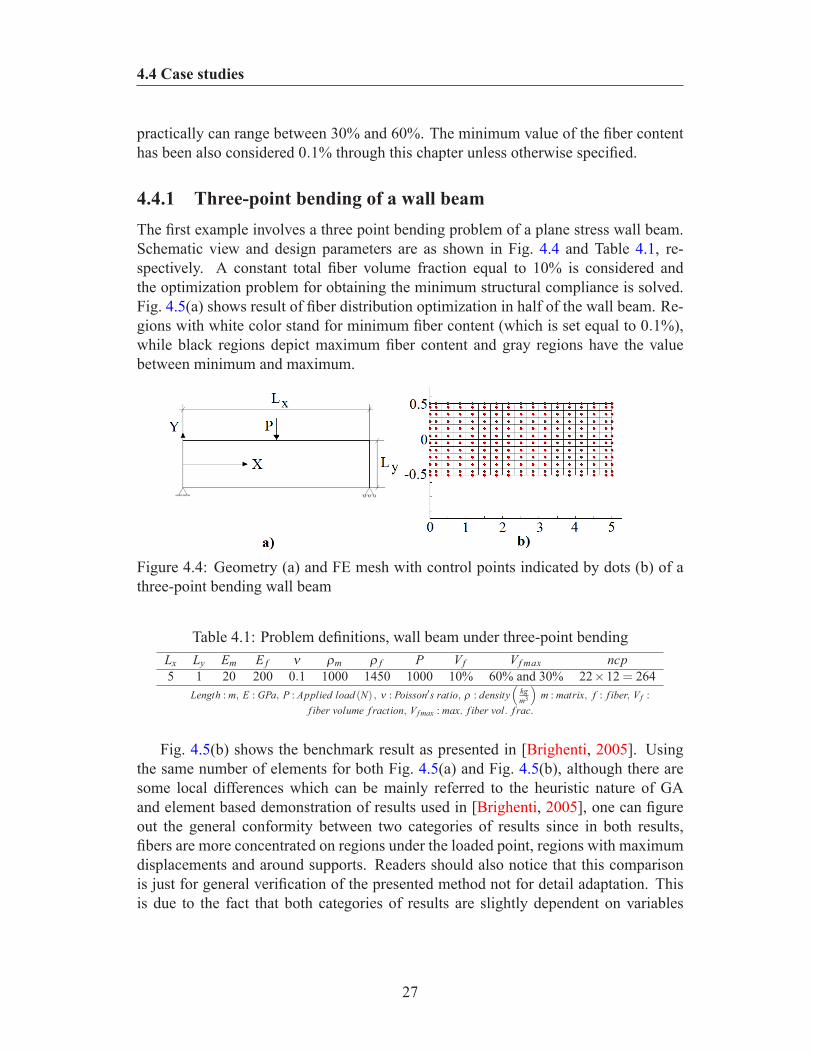
4.4.1 Three-point bending of a wall beamThe first example involves a three point bending problem of a plane stress wall beam.Schematic view and design parameters are as shown in Fig. 4.4 and Table 4.1, re-spectively. A constant total fiber volume fraction equal to 10% is considered andthe optimization problem for obtaining the minimum structural compliance is solved.Fig. 4.5(a) shows result of fiber distribution optimization in half of the wall beam. Re-gions with white color stand for minimum fiber content (which is set equal to 0.1%),while black regions depict maximum fiber content and gray regions have the valuebetween minimum and maximum.
Figure 4.4: Geometry (a) and FE mesh with control points indicated by dots (b) of athree-point bending wall beam
Table 4.1: Problem definitions, wall beam under three-point bendingLx Ly Em E f ν ρm ρ f P Vf Vf max ncp5 1 20 200 0.1 1000 1450 1000 10% 60% and 30% 22×12 = 264
Length : m, E : GPa, P : Applied load (N) , ν : Poisson′s ratio, ρ : density(
kgm3
)m : matrix, f : f iber, V f :
f iber volume f raction, V f max : max. f iber vol. f rac.
Fig. 4.5(b) shows the benchmark result as presented in [Brighenti, 2005]. Usingthe same number of elements for both Fig. 4.5(a) and Fig. 4.5(b), although there aresome local differences which can be mainly referred to the heuristic nature of GAand element based demonstration of results used in [Brighenti, 2005], one can figureout the general conformity between two categories of results since in both results,fibers are more concentrated on regions under the loaded point, regions with maximumdisplacements and around supports. Readers should also notice that this comparisonis just for general verification of the presented method not for detail adaptation. Thisis due to the fact that both categories of results are slightly dependent on variables
27
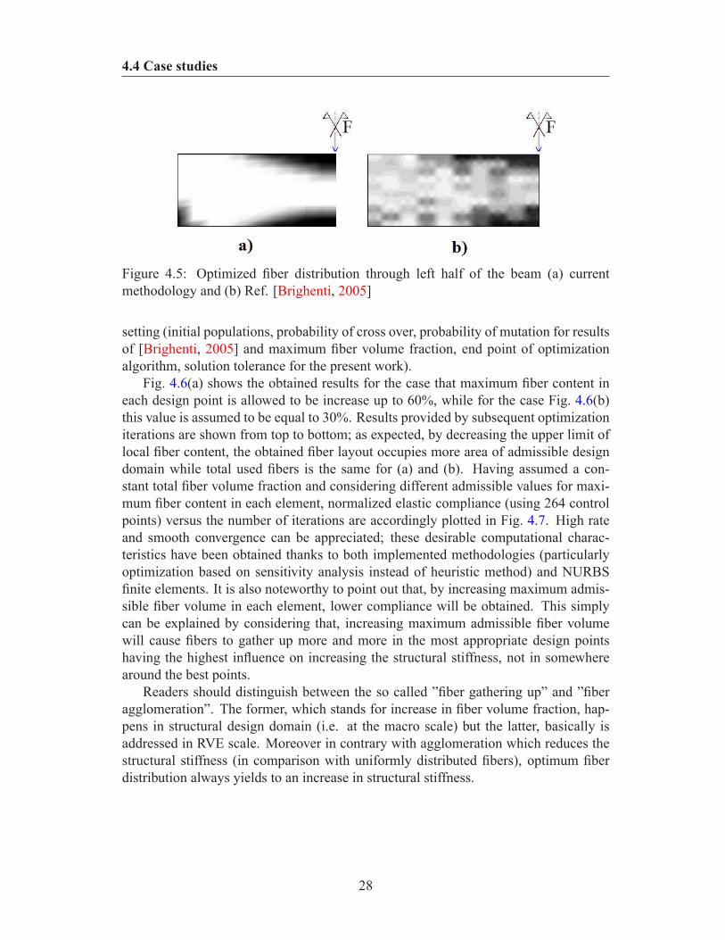
4.4 Case studies
Figure 4.5: Optimized fiber distribution through left half of the beam (a) currentmethodology and (b) Ref. [Brighenti, 2005]
setting (initial populations, probability of cross over, probability of mutation for resultsof [Brighenti, 2005] and maximum fiber volume fraction, end point of optimizationalgorithm, solution tolerance for the present work).
Fig. 4.6(a) shows the obtained results for the case that maximum fiber content ineach design point is allowed to be increase up to 60%, while for the case Fig. 4.6(b)this value is assumed to be equal to 30%. Results provided by subsequent optimizationiterations are shown from top to bottom; as expected, by decreasing the upper limit oflocal fiber content, the obtained fiber layout occupies more area of admissible designdomain while total used fibers is the same for (a) and (b). Having assumed a con-stant total fiber volume fraction and considering different admissible values for maxi-mum fiber content in each element, normalized elastic compliance (using 264 controlpoints) versus the number of iterations are accordingly plotted in Fig. 4.7. High rateand smooth convergence can be appreciated; these desirable computational charac-teristics have been obtained thanks to both implemented methodologies (particularlyoptimization based on sensitivity analysis instead of heuristic method) and NURBSfinite elements. It is also noteworthy to point out that, by increasing maximum admis-sible fiber volume in each element, lower compliance will be obtained. This simplycan be explained by considering that, increasing maximum admissible fiber volumewill cause fibers to gather up more and more in the most appropriate design pointshaving the highest influence on increasing the structural stiffness, not in somewherearound the best points.
Readers should distinguish between the so called ”fiber gathering up” and ”fiberagglomeration”. The former, which stands for increase in fiber volume fraction, hap-pens in structural design domain (i.e. at the macro scale) but the latter, basically isaddressed in RVE scale. Moreover in contrary with agglomeration which reduces thestructural stiffness (in comparison with uniformly distributed fibers), optimum fiberdistribution always yields to an increase in structural stiffness.
28
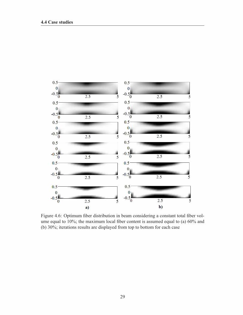
4.4 Case studies
Figure 4.6: Optimum fiber distribution in beam considering a constant total fiber vol-ume equal to 10%; the maximum local fiber content is assumed equal to (a) 60% and(b) 30%; iterations results are displayed from top to bottom for each case
29

4.4 Case studies
Figure 4.7: Normalized compliance versus number of iterations for different values ofmaximum fiber content in each element, using 264 control points
4.4.2 Free vibration of a beamIn the second example free vibration of a FRC beam under different support conditionshas been considered. As indicated in Fig. 4.8 a cantilever beam (Fig. 4.8(a)) and aclamped beam (Fig. 4.8(b)) have been assumed. Design parameters are according toTable 4.2 and FE discretization is the same as in the previous example.
Figure 4.8: Schematic view of problem geometry, (a) cantilever beam (b) clampedbeam
Table 4.2: Problem definitions, free vibration of a beam.Lx Ly Em E f ν ρm ρ f Vf Vf max ncp8 1 20 200 0.1 1000 1450 10% 60% 22×12 = 264
Length : m, E : GPa, ν : Poisson′s ratio, ρ : density(
kgm3
), m : matrix, f : f iber, V f : f iber volume f raction, V f max :
max. f iber vol. f rac.
In this problem the adopted objective function aims to get the maximum value ofthe fundamental frequency by optimizing fiber distribution through the beam domain.
30
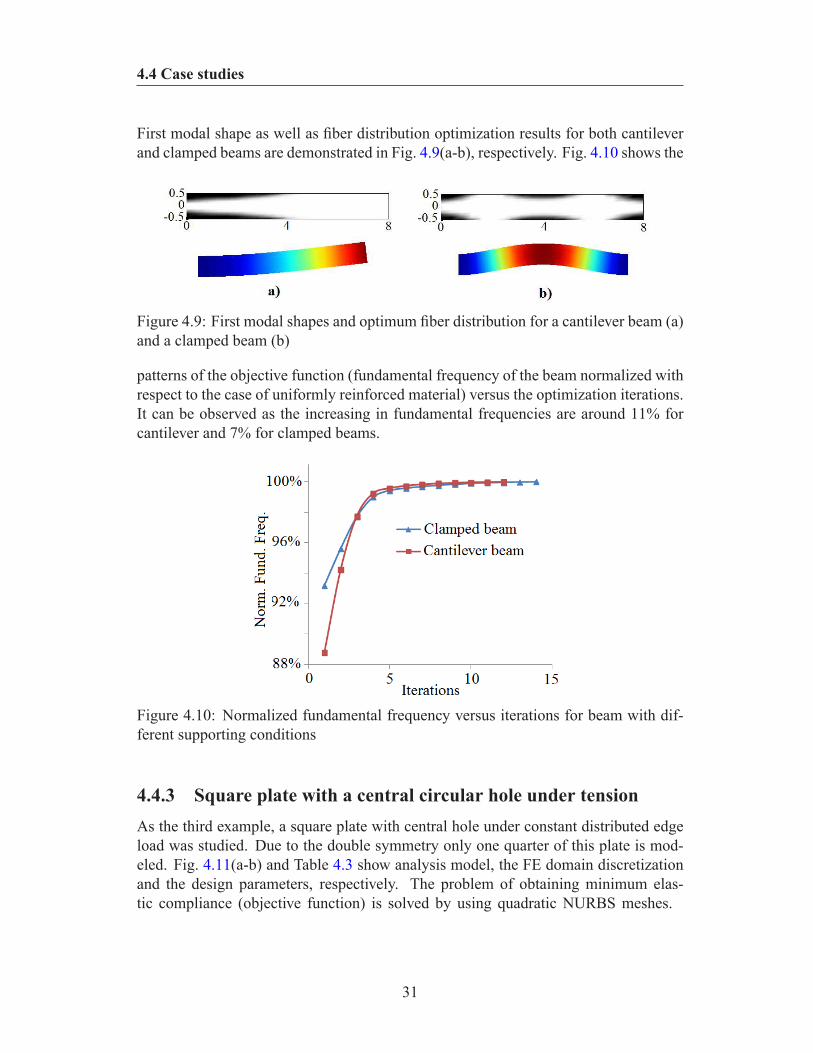
4.4 Case studies
First modal shape as well as fiber distribution optimization results for both cantileverand clamped beams are demonstrated in Fig. 4.9(a-b), respectively. Fig. 4.10 shows the
Figure 4.9: First modal shapes and optimum fiber distribution for a cantilever beam (a)and a clamped beam (b)
patterns of the objective function (fundamental frequency of the beam normalized withrespect to the case of uniformly reinforced material) versus the optimization iterations.It can be observed as the increasing in fundamental frequencies are around 11% forcantilever and 7% for clamped beams.
Figure 4.10: Normalized fundamental frequency versus iterations for beam with dif-ferent supporting conditions
4.4.3 Square plate with a central circular hole under tensionAs the third example, a square plate with central hole under constant distributed edgeload was studied. Due to the double symmetry only one quarter of this plate is mod-eled. Fig. 4.11(a-b) and Table 4.3 show analysis model, the FE domain discretizationand the design parameters, respectively. The problem of obtaining minimum elas-tic compliance (objective function) is solved by using quadratic NURBS meshes.
31
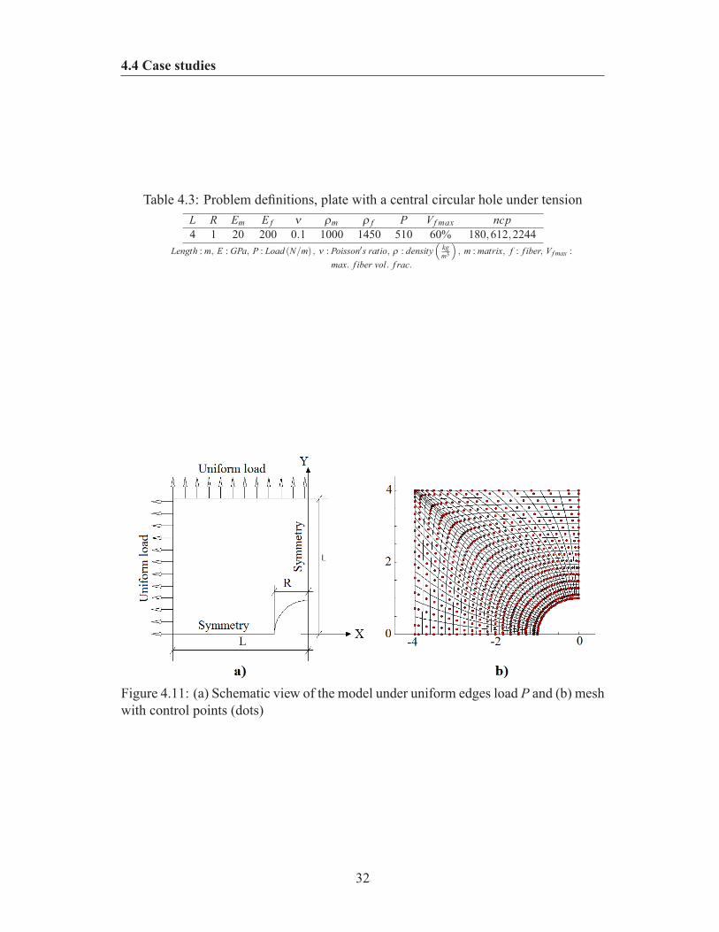
4.4 Case studies
Table 4.3: Problem definitions, plate with a central circular hole under tensionL R Em E f ν ρm ρ f P Vf max ncp4 1 20 200 0.1 1000 1450 510 60% 180,612,2244
Length : m, E : GPa, P : Load (N/m) , ν : Poisson′s ratio, ρ : density(
kgm3
), m : matrix, f : f iber, V f max :
max. f iber vol. f rac.
Figure 4.11: (a) Schematic view of the model under uniform edges load P and (b) meshwith control points (dots)
32
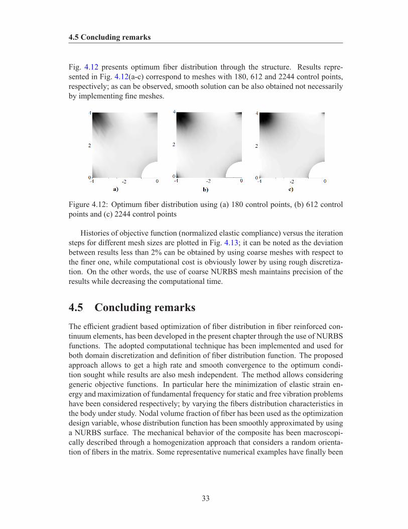
4.5 Concluding remarks
Fig. 4.12 presents optimum fiber distribution through the structure. Results repre-sented in Fig. 4.12(a-c) correspond to meshes with 180, 612 and 2244 control points,respectively; as can be observed, smooth solution can be also obtained not necessarilyby implementing fine meshes.
Figure 4.12: Optimum fiber distribution using (a) 180 control points, (b) 612 controlpoints and (c) 2244 control points
Histories of objective function (normalized elastic compliance) versus the iterationsteps for different mesh sizes are plotted in Fig. 4.13; it can be noted as the deviationbetween results less than 2% can be obtained by using coarse meshes with respect tothe finer one, while computational cost is obviously lower by using rough discretiza-tion. On the other words, the use of coarse NURBS mesh maintains precision of theresults while decreasing the computational time.
4.5 Concluding remarksThe efficient gradient based optimization of fiber distribution in fiber reinforced con-tinuum elements, has been developed in the present chapter through the use of NURBSfunctions. The adopted computational technique has been implemented and used forboth domain discretization and definition of fiber distribution function. The proposedapproach allows to get a high rate and smooth convergence to the optimum condi-tion sought while results are also mesh independent. The method allows consideringgeneric objective functions. In particular here the minimization of elastic strain en-ergy and maximization of fundamental frequency for static and free vibration problemshave been considered respectively; by varying the fibers distribution characteristics inthe body under study. Nodal volume fraction of fiber has been used as the optimizationdesign variable, whose distribution function has been smoothly approximated by usinga NURBS surface. The mechanical behavior of the composite has been macroscopi-cally described through a homogenization approach that considers a random orienta-tion of fibers in the matrix. Some representative numerical examples have finally been
33
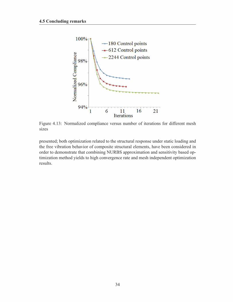
4.5 Concluding remarks
Figure 4.13: Normalized compliance versus number of iterations for different meshsizes
presented; both optimization related to the structural response under static loading andthe free vibration behavior of composite structural elements, have been considered inorder to demonstrate that combining NURBS approximation and sensitivity based op-timization method yields to high convergence rate and mesh independent optimizationresults.
34
Chapter 5
Uncertainties propagation inoptimization of CNT/polymercomposite
5.1 IntroductionCarbon Nano Tube (CNT) in polymer matrix which is called CNT/polymer compos-ites have received attention thanks to their enhanced mechanical, electrical and thermalproperties [Lau et al., 2006]. Different approaches have been used in order to charac-terize Polymeric Nano Composites (PNCs): atomistic modeling, continuum modeling(which can be also subdivided into analytical and numerical approaches) and multi-scale methods [Shokrieh & Rafiee, 2010c]. Molecular dynamics (MD) simulationsrestrict the model to one CNT in a polymer matrix with very short length. Pure contin-uum modeling approaches which usually deal with evaluating the composite responsein the scale of a Representative Volume Element (RVE), do not account for phenomenataking place on finer scales. Therefore, multi-scale methods were employed couplingMD methods and continuum methods. An overview of multi-scale methods for PNCshas been presented in [Shokrieh & Rafiee, 2012].
The characteristics of a Carbon Nano Tube Reinforced Polymer (CNTRP) mate-rial are influenced by many uncertainties. These uncertainties include material prop-erties, the geometry, loading and boundary conditions and the model uncertainties.Hence, probabilistic approaches are needed to determine the reliability of the behaviorof nanocomposite structures.
In this chapter, uncertainties are classified in three major groups: material uncer-tainties, structural uncertainties and modeling uncertainties (Fig. 5.1). Material un-certainties include the molecular interactions and the CNT diameter at nano-scale, theCNT length and CNT-resin interaction at micro-scale, the CNT content, agglomera-
35
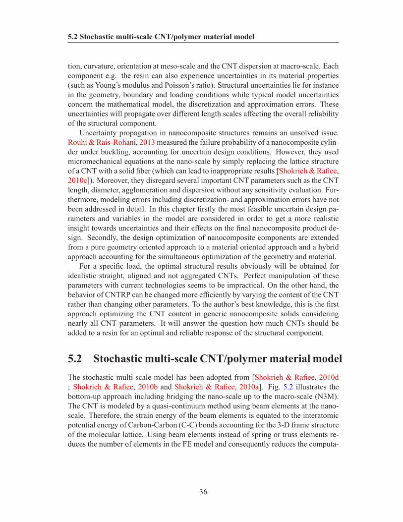
5.2 Stochastic multi-scale CNT/polymer material model
tion, curvature, orientation at meso-scale and the CNT dispersion at macro-scale. Eachcomponent e.g. the resin can also experience uncertainties in its material properties(such as Young’s modulus and Poisson’s ratio). Structural uncertainties lie for instancein the geometry, boundary and loading conditions while typical model uncertaintiesconcern the mathematical model, the discretization and approximation errors. Theseuncertainties will propagate over different length scales affecting the overall reliabilityof the structural component.
Uncertainty propagation in nanocomposite structures remains an unsolved issue.Rouhi & Rais-Rohani, 2013 measured the failure probability of a nanocomposite cylin-der under buckling, accounting for uncertain design conditions. However, they usedmicromechanical equations at the nano-scale by simply replacing the lattice structureof a CNT with a solid fiber (which can lead to inappropriate results [Shokrieh & Rafiee,2010c]). Moreover, they disregard several important CNT parameters such as the CNTlength, diameter, agglomeration and dispersion without any sensitivity evaluation. Fur-thermore, modeling errors including discretization- and approximation errors have notbeen addressed in detail. In this chapter firstly the most feasible uncertain design pa-rameters and variables in the model are considered in order to get a more realisticinsight towards uncertainties and their effects on the final nanocomposite product de-sign. Secondly, the design optimization of nanocomposite components are extendedfrom a pure geometry oriented approach to a material oriented approach and a hybridapproach accounting for the simultaneous optimization of the geometry and material.
For a specific load, the optimal structural results obviously will be obtained foridealistic straight, aligned and not aggregated CNTs. Perfect manipulation of theseparameters with current technologies seems to be impractical. On the other hand, thebehavior of CNTRP can be changed more efficiently by varying the content of the CNTrather than changing other parameters. To the author’s best knowledge, this is the firstapproach optimizing the CNT content in generic nanocomposite solids consideringnearly all CNT parameters. It will answer the question how much CNTs should beadded to a resin for an optimal and reliable response of the structural component.
5.2 Stochastic multi-scale CNT/polymer material modelThe stochastic multi-scale model has been adopted from [Shokrieh & Rafiee, 2010d; Shokrieh & Rafiee, 2010b and Shokrieh & Rafiee, 2010a]. Fig. 5.2 illustrates thebottom-up approach including bridging the nano-scale up to the macro-scale (N3M).The CNT is modeled by a quasi-continuum method using beam elements at the nano-scale. Therefore, the strain energy of the beam elements is equated to the interatomicpotential energy of Carbon-Carbon (C-C) bonds accounting for the 3-D frame structureof the molecular lattice. Using beam elements instead of spring or truss elements re-duces the number of elements in the FE model and consequently reduces the computa-
36

5.2 Stochastic multi-scale CNT/polymer material model
Figure 5.1: Uncertainties sources and their propagation over different length scales andsources
37
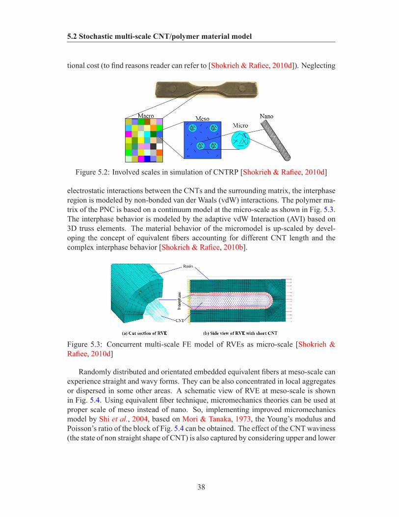
5.2 Stochastic multi-scale CNT/polymer material model
tional cost (to find reasons reader can refer to [Shokrieh & Rafiee, 2010d]). Neglecting
Figure 5.2: Involved scales in simulation of CNTRP [Shokrieh & Rafiee, 2010d]
electrostatic interactions between the CNTs and the surrounding matrix, the interphaseregion is modeled by non-bonded van der Waals (vdW) interactions. The polymer ma-trix of the PNC is based on a continuum model at the micro-scale as shown in Fig. 5.3.The interphase behavior is modeled by the adaptive vdW Interaction (AVI) based on3D truss elements. The material behavior of the micromodel is up-scaled by devel-oping the concept of equivalent fibers accounting for different CNT length and thecomplex interphase behavior [Shokrieh & Rafiee, 2010b].
Figure 5.3: Concurrent multi-scale FE model of RVEs as micro-scale [Shokrieh &Rafiee, 2010d]
Randomly distributed and orientated embedded equivalent fibers at meso-scale canexperience straight and wavy forms. They can be also concentrated in local aggregatesor dispersed in some other areas. A schematic view of RVE at meso-scale is shownin Fig. 5.4. Using equivalent fiber technique, micromechanics theories can be used atproper scale of meso instead of nano. So, implementing improved micromechanicsmodel by Shi et al., 2004, based on Mori & Tanaka, 1973, the Young’s modulus andPoisson’s ratio of the block of Fig. 5.4 can be obtained. The effect of the CNT waviness(the state of non straight shape of CNT) is also captured by considering upper and lower
38
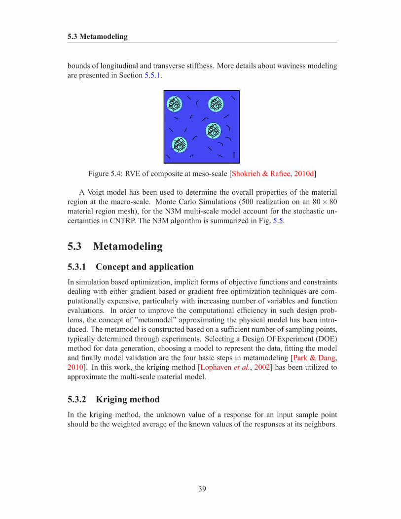
5.3 Metamodeling
bounds of longitudinal and transverse stiffness. More details about waviness modelingare presented in Section 5.5.1.
Figure 5.4: RVE of composite at meso-scale [Shokrieh & Rafiee, 2010d]
A Voigt model has been used to determine the overall properties of the materialregion at the macro-scale. Monte Carlo Simulations (500 realization on an 80× 80material region mesh), for the N3M multi-scale model account for the stochastic un-certainties in CNTRP. The N3M algorithm is summarized in Fig. 5.5.
5.3 Metamodeling
5.3.1 Concept and applicationIn simulation based optimization, implicit forms of objective functions and constraintsdealing with either gradient based or gradient free optimization techniques are com-putationally expensive, particularly with increasing number of variables and functionevaluations. In order to improve the computational efficiency in such design prob-lems, the concept of ”metamodel” approximating the physical model has been intro-duced. The metamodel is constructed based on a sufficient number of sampling points,typically determined through experiments. Selecting a Design Of Experiment (DOE)method for data generation, choosing a model to represent the data, fitting the modeland finally model validation are the four basic steps in metamodeling [Park & Dang,2010]. In this work, the kriging method [Lophaven et al., 2002] has been utilized toapproximate the multi-scale material model.
5.3.2 Kriging methodIn the kriging method, the unknown value of a response for an input sample pointshould be the weighted average of the known values of the responses at its neighbors.
39
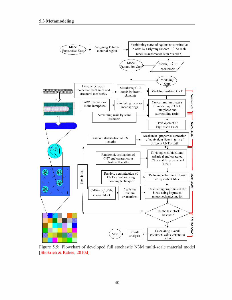
5.3 Metamodeling
Figure 5.5: Flowchart of developed full stochastic N3M multi-scale material model[Shokrieh & Rafiee, 2010d]
40
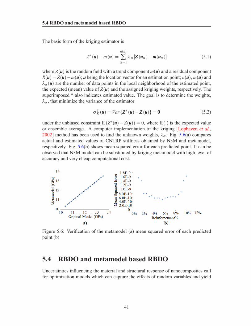
5.4 RBDO and metamodel based RBDO
The basic form of the kriging estimator is
Z∗ (uuu)−m(uuu) =n(u)
∑α=1
λα [ZZZ (uuuα)−mmm(uuuα)] (5.1)
where Z(uuu) is the random field with a trend component m(uuu) and a residual componentR(uuu) = Z(uuu)−m(uuu); uuu being the location vector for an estimation point; n(uuu), m(uuu) andλα(uuu) are the number of data points in the local neighborhood of the estimated point,the expected (mean) value of Z(uuu) and the assigned kriging weights, respectively. Thesuperimposed * also indicates estimated value. The goal is to determine the weights,λα , that minimize the variance of the estimator
σ2E (uuu) =VarZZZ∗ (uuu)−ZZZ (uuu)= 000 (5.2)
under the unbiased constraint E(Z∗(uuu)−Z(uuu)) = 0, where E(.) is the expected valueor ensemble average. A computer implementation of the kriging [Lophaven et al.,2002] method has been used to find the unknown weights, λα . Fig. 5.6(a) comparesactual and estimated values of CNTRP stiffness obtained by N3M and metamodel,respectively. Fig. 5.6(b) shows mean squared error for each predicted point. It can beobserved that N3M model can be substituted by kriging metamodel with high level ofaccuracy and very cheap computational cost.
Figure 5.6: Verification of the metamodel (a) mean squared error of each predictedpoint (b)
5.4 RBDO and metamodel based RBDOUncertainties influencing the material and structural response of nanocomposites callfor optimization models which can capture the effects of random variables and yield
41
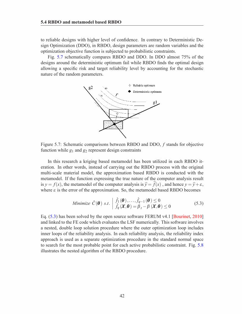
5.4 RBDO and metamodel based RBDO
to reliable designs with higher level of confidence. In contrary to Deterministic De-sign Optimization (DDO), in RBDO, design parameters are random variables and theoptimization objective function is subjected to probabilistic constraints.
Fig. 5.7 schematically compares RBDO and DDO. In DDO almost 75% of thedesigns around the deterministic optimum fail while RBDO finds the optimal designallowing a specific risk and target reliability level by accounting for the stochasticnature of the random parameters.
Figure 5.7: Schematic comparisons between RBDO and DDO, f stands for objectivefunction while g1 and g2 represent design constraints
In this research a kriging based metamodel has been utilized in each RBDO it-eration. In other words, instead of carrying out the RBDO process with the originalmulti-scale material model, the approximation based RBDO is conducted with themetamodel. If the function expressing the true nature of the computer analysis resultis y = f (x), the metamodel of the computer analysis is y = f (x) , and hence y = y+ ε ,where ε is the error of the approximation. So, the metamodel based RBDO becomes
Minimize C (θθθ) s.t.∣∣∣∣
f1 (θθθ) , . . . , fq−1 (θθθ)≤ 0fq (XXX ,θθθ) = β t −β (XXX ,θθθ)≤ 0 (5.3)
Eq. (5.3) has been solved by the open source software FERUM v4.1 [Bourinet, 2010]and linked to the FE code which evaluates the LSF numerically. This software involvesa nested, double loop solution procedure where the outer optimization loop includesinner loops of the reliability analysis. In each reliability analysis, the reliability indexapproach is used as a separate optimization procedure in the standard normal spaceto search for the most probable point for each active probabilistic constraint. Fig. 5.8illustrates the nested algorithm of the RBDO procedure.
42
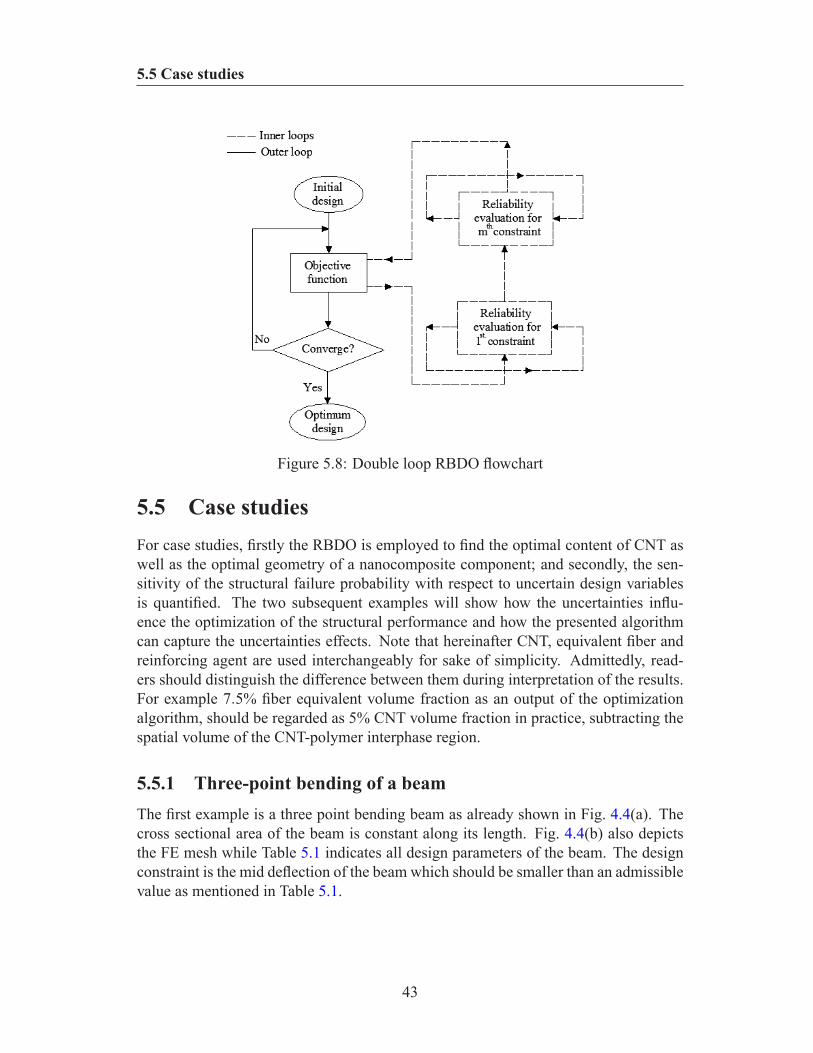
5.5 Case studies
Figure 5.8: Double loop RBDO flowchart
5.5 Case studiesFor case studies, firstly the RBDO is employed to find the optimal content of CNT aswell as the optimal geometry of a nanocomposite component; and secondly, the sen-sitivity of the structural failure probability with respect to uncertain design variablesis quantified. The two subsequent examples will show how the uncertainties influ-ence the optimization of the structural performance and how the presented algorithmcan capture the uncertainties effects. Note that hereinafter CNT, equivalent fiber andreinforcing agent are used interchangeably for sake of simplicity. Admittedly, read-ers should distinguish the difference between them during interpretation of the results.For example 7.5% fiber equivalent volume fraction as an output of the optimizationalgorithm, should be regarded as 5% CNT volume fraction in practice, subtracting thespatial volume of the CNT-polymer interphase region.
5.5.1 Three-point bending of a beamThe first example is a three point bending beam as already shown in Fig. 4.4(a). Thecross sectional area of the beam is constant along its length. Fig. 4.4(b) also depictsthe FE mesh while Table 5.1 indicates all design parameters of the beam. The designconstraint is the mid deflection of the beam which should be smaller than an admissiblevalue as mentioned in Table 5.1.
43
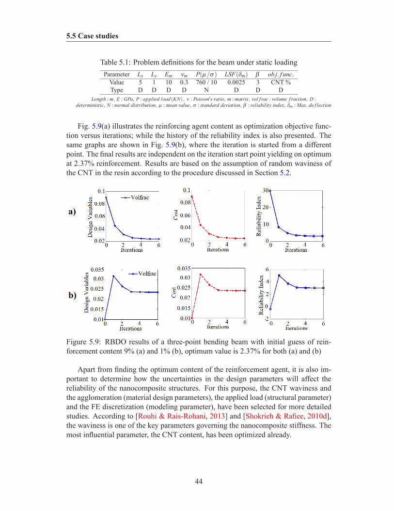
5.5 Case studies
Table 5.1: Problem definitions for the beam under static loadingParameter Lx Ly Em νm P(µ/σ) LSF(δm) β ob j. f unc.
Value 5 1 10 0.3 760 / 10 0.0025 3 CNT %Type D D D D N D D D
Length : m, E : GPa, P : applied load (KN) , ν : Poisson′s ratio, m : matrix, vol f rac : volume f raction, D :deterministic, N : normal distribution, µ : mean value, σ : standard deviation, β : reliability index, δm : Max. de f lection
Fig. 5.9(a) illustrates the reinforcing agent content as optimization objective func-tion versus iterations; while the history of the reliability index is also presented. Thesame graphs are shown in Fig. 5.9(b), where the iteration is started from a differentpoint. The final results are independent on the iteration start point yielding on optimumat 2.37% reinforcement. Results are based on the assumption of random waviness ofthe CNT in the resin according to the procedure discussed in Section 5.2.
Figure 5.9: RBDO results of a three-point bending beam with initial guess of rein-forcement content 9% (a) and 1% (b), optimum value is 2.37% for both (a) and (b)
Apart from finding the optimum content of the reinforcement agent, it is also im-portant to determine how the uncertainties in the design parameters will affect thereliability of the nanocomposite structures. For this purpose, the CNT waviness andthe agglomeration (material design parameters), the applied load (structural parameter)and the FE discretization (modeling parameter), have been selected for more detailedstudies. According to [Rouhi & Rais-Rohani, 2013] and [Shokrieh & Rafiee, 2010d],the waviness is one of the key parameters governing the nanocomposite stiffness. Themost influential parameter, the CNT content, has been optimized already.
44
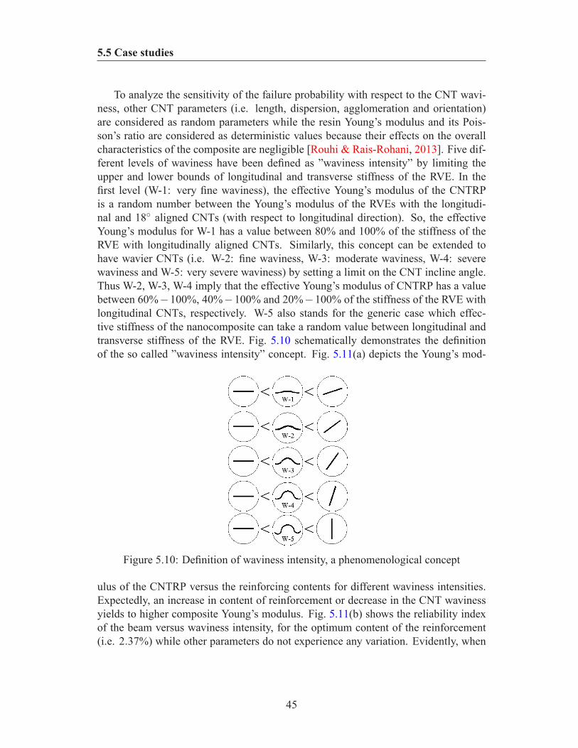
5.5 Case studies
To analyze the sensitivity of the failure probability with respect to the CNT wavi-ness, other CNT parameters (i.e. length, dispersion, agglomeration and orientation)are considered as random parameters while the resin Young’s modulus and its Pois-son’s ratio are considered as deterministic values because their effects on the overallcharacteristics of the composite are negligible [Rouhi & Rais-Rohani, 2013]. Five dif-ferent levels of waviness have been defined as ”waviness intensity” by limiting theupper and lower bounds of longitudinal and transverse stiffness of the RVE. In thefirst level (W-1: very fine waviness), the effective Young’s modulus of the CNTRPis a random number between the Young’s modulus of the RVEs with the longitudi-nal and 18 aligned CNTs (with respect to longitudinal direction). So, the effectiveYoung’s modulus for W-1 has a value between 80% and 100% of the stiffness of theRVE with longitudinally aligned CNTs. Similarly, this concept can be extended tohave wavier CNTs (i.e. W-2: fine waviness, W-3: moderate waviness, W-4: severewaviness and W-5: very severe waviness) by setting a limit on the CNT incline angle.Thus W-2, W-3, W-4 imply that the effective Young’s modulus of CNTRP has a valuebetween 60%−100%, 40%−100% and 20%−100% of the stiffness of the RVE withlongitudinal CNTs, respectively. W-5 also stands for the generic case which effec-tive stiffness of the nanocomposite can take a random value between longitudinal andtransverse stiffness of the RVE. Fig. 5.10 schematically demonstrates the definitionof the so called ”waviness intensity” concept. Fig. 5.11(a) depicts the Young’s mod-
Figure 5.10: Definition of waviness intensity, a phenomenological concept
ulus of the CNTRP versus the reinforcing contents for different waviness intensities.Expectedly, an increase in content of reinforcement or decrease in the CNT wavinessyields to higher composite Young’s modulus. Fig. 5.11(b) shows the reliability indexof the beam versus waviness intensity, for the optimum content of the reinforcement(i.e. 2.37%) while other parameters do not experience any variation. Evidently, when
45
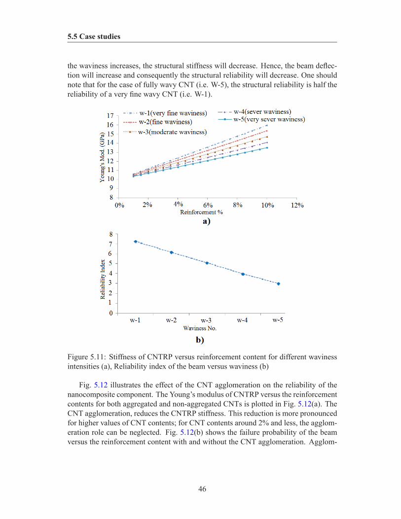
5.5 Case studies
the waviness increases, the structural stiffness will decrease. Hence, the beam deflec-tion will increase and consequently the structural reliability will decrease. One shouldnote that for the case of fully wavy CNT (i.e. W-5), the structural reliability is half thereliability of a very fine wavy CNT (i.e. W-1).
Figure 5.11: Stiffness of CNTRP versus reinforcement content for different wavinessintensities (a), Reliability index of the beam versus waviness (b)
Fig. 5.12 illustrates the effect of the CNT agglomeration on the reliability of thenanocomposite component. The Young’s modulus of CNTRP versus the reinforcementcontents for both aggregated and non-aggregated CNTs is plotted in Fig. 5.12(a). TheCNT agglomeration, reduces the CNTRP stiffness. This reduction is more pronouncedfor higher values of CNT contents; for CNT contents around 2% and less, the agglom-eration role can be neglected. Fig. 5.12(b) shows the failure probability of the beamversus the reinforcement content with and without the CNT agglomeration. Agglom-
46
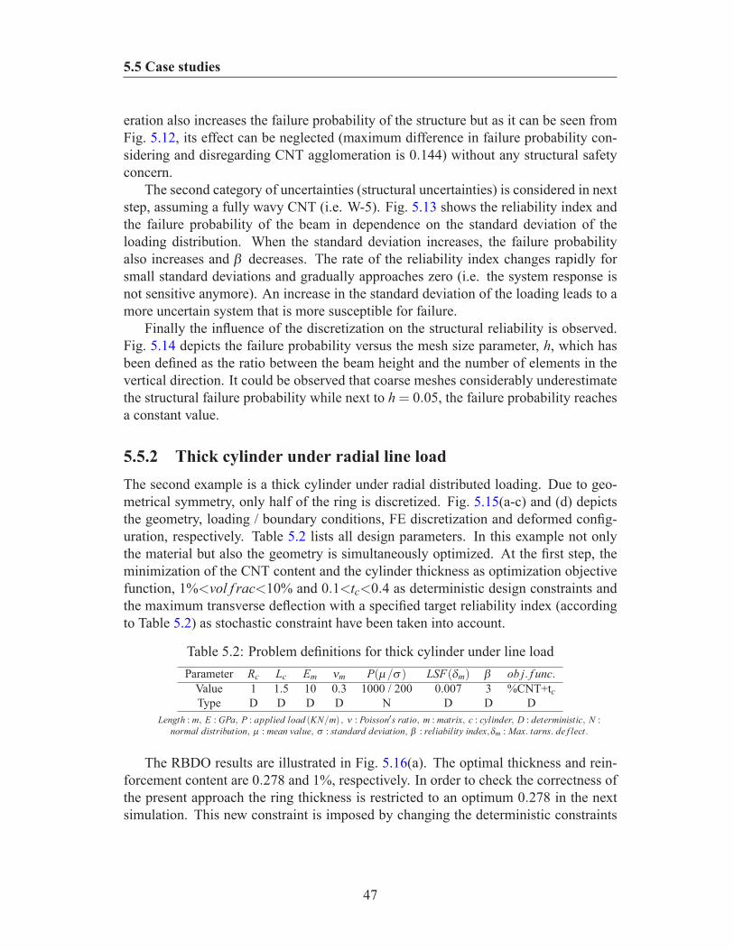
5.5 Case studies
eration also increases the failure probability of the structure but as it can be seen fromFig. 5.12, its effect can be neglected (maximum difference in failure probability con-sidering and disregarding CNT agglomeration is 0.144) without any structural safetyconcern.
The second category of uncertainties (structural uncertainties) is considered in nextstep, assuming a fully wavy CNT (i.e. W-5). Fig. 5.13 shows the reliability index andthe failure probability of the beam in dependence on the standard deviation of theloading distribution. When the standard deviation increases, the failure probabilityalso increases and β decreases. The rate of the reliability index changes rapidly forsmall standard deviations and gradually approaches zero (i.e. the system response isnot sensitive anymore). An increase in the standard deviation of the loading leads to amore uncertain system that is more susceptible for failure.
Finally the influence of the discretization on the structural reliability is observed.Fig. 5.14 depicts the failure probability versus the mesh size parameter, h, which hasbeen defined as the ratio between the beam height and the number of elements in thevertical direction. It could be observed that coarse meshes considerably underestimatethe structural failure probability while next to h = 0.05, the failure probability reachesa constant value.
5.5.2 Thick cylinder under radial line loadThe second example is a thick cylinder under radial distributed loading. Due to geo-metrical symmetry, only half of the ring is discretized. Fig. 5.15(a-c) and (d) depictsthe geometry, loading / boundary conditions, FE discretization and deformed config-uration, respectively. Table 5.2 lists all design parameters. In this example not onlythe material but also the geometry is simultaneously optimized. At the first step, theminimization of the CNT content and the cylinder thickness as optimization objectivefunction, 1%<vol f rac<10% and 0.1<tc<0.4 as deterministic design constraints andthe maximum transverse deflection with a specified target reliability index (accordingto Table 5.2) as stochastic constraint have been taken into account.
Table 5.2: Problem definitions for thick cylinder under line loadParameter Rc Lc Em νm P(µ/σ) LSF(δm) β ob j. f unc.
Value 1 1.5 10 0.3 1000 / 200 0.007 3 %CNT+tcType D D D D N D D D
Length : m, E : GPa, P : applied load (KN/m) , ν : Poisson′s ratio, m : matrix, c : cylinder, D : deterministic, N :normal distribution, µ : mean value, σ : standard deviation, β : reliability index,δm : Max. tarns. de f lect.
The RBDO results are illustrated in Fig. 5.16(a). The optimal thickness and rein-forcement content are 0.278 and 1%, respectively. In order to check the correctness ofthe present approach the ring thickness is restricted to an optimum 0.278 in the nextsimulation. This new constraint is imposed by changing the deterministic constraints
47
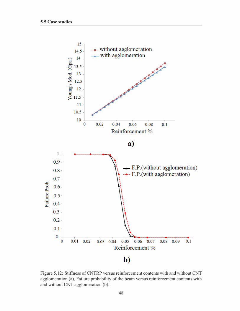
5.5 Case studies
Figure 5.12: Stiffness of CNTRP versus reinforcement contents with and without CNTagglomeration (a), Failure probability of the beam versus reinforcement contents withand without CNT agglomeration (b).
48
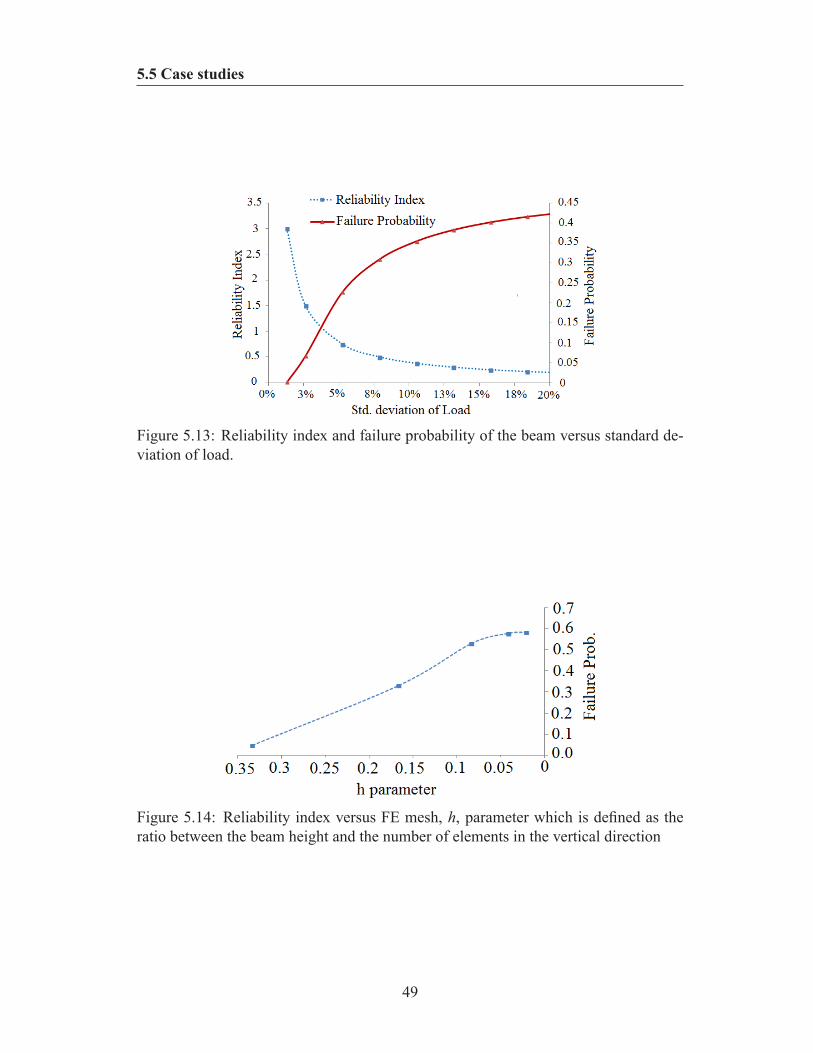
5.5 Case studies
Figure 5.13: Reliability index and failure probability of the beam versus standard de-viation of load.
Figure 5.14: Reliability index versus FE mesh, h, parameter which is defined as theratio between the beam height and the number of elements in the vertical direction
49
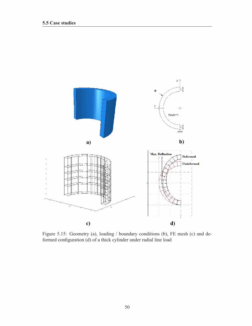
5.5 Case studies
Figure 5.15: Geometry (a), loading / boundary conditions (b), FE mesh (c) and de-formed configuration (d) of a thick cylinder under radial line load
50
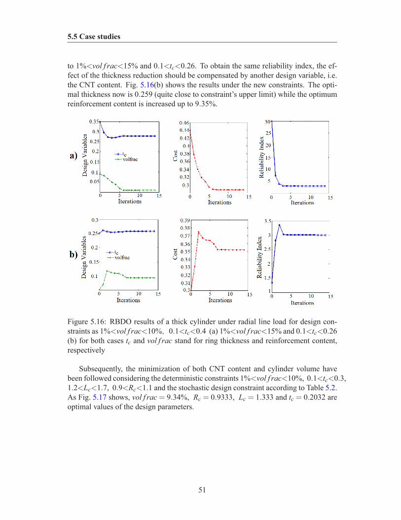
5.5 Case studies
to 1%<vol f rac<15% and 0.1<tc<0.26. To obtain the same reliability index, the ef-fect of the thickness reduction should be compensated by another design variable, i.e.the CNT content. Fig. 5.16(b) shows the results under the new constraints. The opti-mal thickness now is 0.259 (quite close to constraint’s upper limit) while the optimumreinforcement content is increased up to 9.35%.
Figure 5.16: RBDO results of a thick cylinder under radial line load for design con-straints as 1%<vol f rac<10%, 0.1<tc<0.4 (a) 1%<vol f rac<15% and 0.1<tc<0.26(b) for both cases tc and vol f rac stand for ring thickness and reinforcement content,respectively
Subsequently, the minimization of both CNT content and cylinder volume havebeen followed considering the deterministic constraints 1%<vol f rac<10%, 0.1<tc<0.3,1.2<Lc<1.7, 0.9<Rc<1.1 and the stochastic design constraint according to Table 5.2.As Fig. 5.17 shows, vol f rac = 9.34%, Rc = 0.9333, Lc = 1.333 and tc = 0.2032 areoptimal values of the design parameters.
51
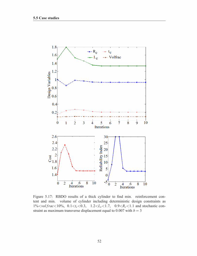
5.5 Case studies
Figure 5.17: RBDO results of a thick cylinder to find min. reinforcement con-tent and min. volume of cylinder including deterministic design constraints as1%<vol f rac<10%, 0.1<tc<0.3, 1.2<Lc<1.7, 0.9<Rc<1.1 and stochastic con-straint as maximum transverse displacement equal to 0.007 with b = 3
52

5.6 Concluding remarks
5.6 Concluding remarksDeterministic approaches for nanocomposite modeling and optimization might be un-realistic for certain applications and may yield to either catastrophic failure or unneces-sary conservatism. Although probabilistic approaches can cover uncertainties effects,their implementations do not necessarily yield reliable nanocomposite designs. De-tailed investigations on uncertainties and their propagation should be performed forrealistic and reliable PNC structures. Uncertainty propagation over different lengthscales and through various sources have been addressed for nanocomposite compo-nents. Potential uncertainties have been categorized in material, structural and mod-eling levels. To fully address uncertainties in material level, a stochastic multi-scalematerial model (which includes all important aspects of the CNTRP including CNTlength, orientation, dispersion, agglomeration and waviness, at different length scalesfrom nano-, up to macro-scale) has been utilized. To improve the computational ef-ficiency, the evaluation of material properties has been surrogated by a metamodel.The results for two selected examples show that the failure probability of a polymericnanocomposite structure, strongly depends on the CNT parameters, especially the CNTvolume fraction and the waviness. The influence of the CNT agglomeration is nearlynegligible. It was observed that neglecting the CNT agglomeration can simplify themodel and decrease the computational time without remarkable loss in model accu-racy. Furthermore, the loading condition and discretization affect the reliability ofthe system. Coarse meshes underestimate the failure probability of a beam while finemeshes admittedly increase computational cost. Thus sufficiently refined discretizationshould be investigated in order to have realistic assessment of the reliability of PNCstructures. An increase in the standard deviation of the applied load, which physicallymeans more uncertainties in the system, resulted in the structure with a smaller relia-bility index. Finding the optimal content of CNT was also presented to optimized thematerial instead of the geometry. As a further step forward, concurrent optimization ofmaterial parameters and geometrical parameters (hybrid optimization) was conductedto present a comprehensive solution for current demands in fully optimized designs ofnanocomposite components.
53
Chapter 6
Reliability and NURBS basedsequential optimization approach
6.1 IntroductionGenerally, increasing the fiber volume fraction in a Fiber Reinforced Composite (FRC)material will increase its structural strength and stiffness. However the existence of apractical upper limit should be considered. Normally, composite structural elementsunder mechanical actions have some regions which are on the edge of design con-straints (e.g. the maximum allowable stress is exceeded) and can be identified as fail-ure zones. Usually these failure zones dictate the required content of the reinforcingelement in order to get a properly strengthened overall structure, fulfilling everywherethe design constraints. Considering uniform distribution of fibers through the structure,initially safe regions that already fulfill the design constraints will inevitably increasetheir fiber content. Thus, an efficient optimization approach which seeks towards op-timal fiber content (see Chapter 5) should also pay attention to optimal distributionof fibers in order to strengthen only those portions of the structure (failure zones) forwhich it is necessary to improve their bearing capacity. From the above discussionsit appears that the joint manipulation of these two parameters (i.e. fiber content andits distribution) while available uncertainties are also addressed, will be a necessaryapproach towards more efficient and reliable structural optimization.
6.2 Double sequential stages optimization procedureThe sequential optimization algorithm is schematically illustrated in Fig. 6.1. In thisapproach there are two successive optimization stages. Stage 1 includes a stochasticfiber content optimization algorithm and stage 2 includes a fiber distribution optimizer.In the first stage, based on the nature of the problem, the designer can decide which
54
6.2 Double sequential stages optimization procedure
parameters would be deterministic and which ones probabilistic. He can also set theinitial values of the parameters, variables and solution settings. Traditional RBDO isimplemented by use of a nested or double loop approach. In this method, each stepof the iteration for design optimization involves another loop of iteration for reliabilityanalysis (i.e. FORM). In this stage, minimization of fiber content is considered as op-timization objective function and after convergence, the output is used as the input forthe second stage. In the second stage, NURBS finite elements which are implementedand used for domain discretization, define continuous and smooth mesh independentfiber distribution function by using the nodal volume fractions of fibers as the opti-mization design variables. The second stage is initialized by using the fiber volumefraction value, coming as stage 1. Afterwards Optimality Criteria (OC) updates de-sign variables. This computational procedure is executed iteratively, until no sensiblechanges occur in design variables (See Chapter 4).
In the presented model, two separate reliability indices (β1 and β2) are introduced:β1 is the first stage reliability index (which is used for obtaining optimal fiber volumefraction through the RBDO in stage 1) and the second reliability index, β2, is the targetreliability index of the final optimized structure. β2 represents the reliability index ofthe structure after fiber distribution optimization. β1 is the model input (set by designerat the first run of the algorithm) while β2 is the output of the model. Clearly, β1 <β2because it is supposed that fiber distribution optimization increases the performance(such as the stiffness) of the model and provides a more reliable structure.
It is however possible to implement concurrent approach for coupling stage 1 andstage 2. In the concurrent approach (Fig. 6.2) the fulfillment of the fiber distributionoptimization before evaluation of LSF is necessary in every realization of stage 1.Thus, this alternative method is computationally expensive. To see more clearly theissue, we can assume that the computational parameter of total elapsed time (Ttotal) isproportional to the number of LSF call (n1), each call run time (tLSF ) and the subtotaltime required for fiber distribution optimization (t2). Taking into account the above, forthe sequential model the total time is proportional to the sum of the above mentionedtimes, i.e:
Ttotalse ∝ (n1 × tLSF + t2) (6.1)
while for concurrent model we have:
Ttotalco ∝ [n1 × (tLSF + t2)] (6.2)
as n1>1, thus , Ttotalse is smaller than Ttotalco. We can write:
(Ttotalco −Ttotalse) = ∆T ∝ [(n1 −1)t2] (6.3)
We can use a quantitative example in order to clarify the above issue. A simple casewhere t2 and n1 are equal to 20 minutes and 10 calls respectively, the present model
55
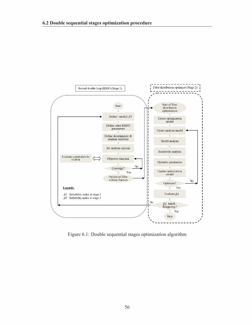
6.2 Double sequential stages optimization procedure
Figure 6.1: Double sequential stages optimization algorithm
56
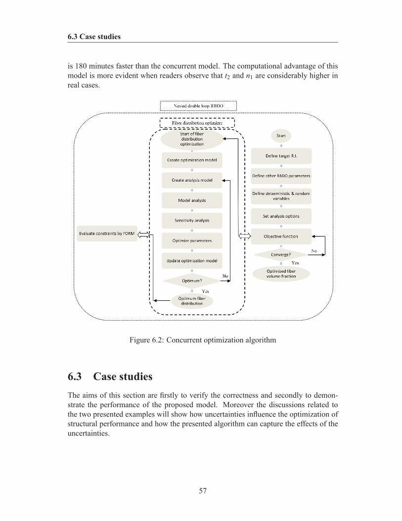
6.3 Case studies
is 180 minutes faster than the concurrent model. The computational advantage of thismodel is more evident when readers observe that t2 and n1 are considerably higher inreal cases.
Figure 6.2: Concurrent optimization algorithm
6.3 Case studiesThe aims of this section are firstly to verify the correctness and secondly to demon-strate the performance of the proposed model. Moreover the discussions related tothe two presented examples will show how uncertainties influence the optimization ofstructural performance and how the presented algorithm can capture the effects of theuncertainties.
57
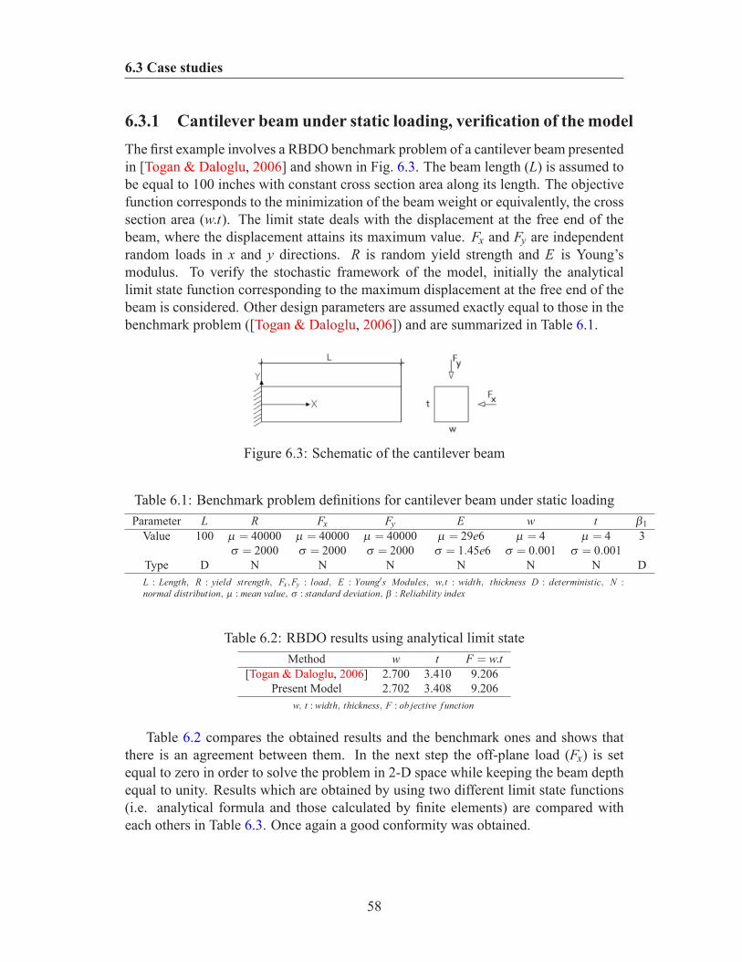
6.3 Case studies
6.3.1 Cantilever beam under static loading, verification of the modelThe first example involves a RBDO benchmark problem of a cantilever beam presentedin [Togan & Daloglu, 2006] and shown in Fig. 6.3. The beam length (L) is assumed tobe equal to 100 inches with constant cross section area along its length. The objectivefunction corresponds to the minimization of the beam weight or equivalently, the crosssection area (w.t). The limit state deals with the displacement at the free end of thebeam, where the displacement attains its maximum value. Fx and Fy are independentrandom loads in x and y directions. R is random yield strength and E is Young’smodulus. To verify the stochastic framework of the model, initially the analyticallimit state function corresponding to the maximum displacement at the free end of thebeam is considered. Other design parameters are assumed exactly equal to those in thebenchmark problem ([Togan & Daloglu, 2006]) and are summarized in Table 6.1.
Figure 6.3: Schematic of the cantilever beam
Table 6.1: Benchmark problem definitions for cantilever beam under static loadingParameter L R Fx Fy E w t β1
Value 100 µ = 40000 µ = 40000 µ = 40000 µ = 29e6 µ = 4 µ = 4 3σ = 2000 σ = 2000 σ = 2000 σ = 1.45e6 σ = 0.001 σ = 0.001
Type D N N N N N N DL : Length, R : yield strength, Fx,Fy : load, E : Young′s Modules, w, t : width, thickness D : deterministic, N :normal distribution, µ : mean value, σ : standard deviation, β : Reliability index
Table 6.2: RBDO results using analytical limit stateMethod w t F = w.t
[Togan & Daloglu, 2006] 2.700 3.410 9.206Present Model 2.702 3.408 9.206
w, t : width, thickness, F : ob jective f unction
Table 6.2 compares the obtained results and the benchmark ones and shows thatthere is an agreement between them. In the next step the off-plane load (Fx) is setequal to zero in order to solve the problem in 2-D space while keeping the beam depthequal to unity. Results which are obtained by using two different limit state functions(i.e. analytical formula and those calculated by finite elements) are compared witheach others in Table 6.3. Once again a good conformity was obtained.
58

6.3 Case studies
Table 6.3: RBDO results using FEM limit stateMethod for evaluation of LSF w t F = w.t
Analytical 1 4.0095 4.0095FEM(NURBS) 1 4.0094 4.0094
w, t : width, thickness, F : ob jective f unction
6.3.2 Beam under three-point bendingIn the present example the first objective function is to find the optimal fiber volumewhile the limit state is the deflection at mid of the beam must be smaller than anadmissible value. The schematic view of the problem is already shown in Fig. 4.4while Table 6.4 includes the design parameters.
Table 6.4: Problem definitions of the beam under static loadingParameter Lx Ly Lm E f ν P LSF β1 Ob j.Func.
Value 5 1 µ = 20 µ = 200 0.1 µ = 1000 Max. Deflect. 3 Fiber Volumeσ = 5 σ = 50 σ = 250 4e−3 fraction
Type D D N N D N D D DLength : (M), E : (MPa), P : applied load(N), ν : Poisson′s ratio, m : matrix, f : f iber, D : deterministic, N :normal distribution, µ : mean value, σ : standard deviation, β1 : reliability index
Fig. 6.4 presents optimal values of fiber volume fraction for the beam with homo-geneously distributed fibers versus the different maximum allowable deflection at midof the beam and for different reliability indices. A mesh with 91 control points hasbeen used to reduce computational cost. As expected, either demanding smaller beamdeflection or greater reliability index for the beam, yield to increase in fiber volumefraction of the FRC beam. The figure also depicts that for large reliability indices(here 4 and 5) and when there is a small allowable beam deflection (here 5 mm), theobtained fiber contents are approximately the same.
Results of RBDO by using 1225 control points, which represents 4120 mesh sizes,are plotted in Fig. 6.5. For this (or higher) number of control points, the numericalsolutions of the LSF have been verified to converge to the exact solution.
Fig. 6.6 compares the obtained values related to the assumed objective function fordifferent numbers of control points (mesh sizes). As can be observed, the deviation be-tween the obtained optimal fiber volume fractions by using 1225 or 325 control pointsis equal to 0.03 (i.e. 3%) but the computational time is reduced to be approximatelyless than one tenth. This fact underlines NURBS smooth and quick convergence char-acteristics which yield to noticeable saving in the time of the computation. In RBDOproblem, LSF which depends on FE model results, should be evaluated many times.So, any reduction in its calculation time will significantly reduce the total elapsed time.Admittedly, this time saving is justified only in the case that accuracy of the results isalso maintained. This takes place in the presented model while using coarse NURBS
59
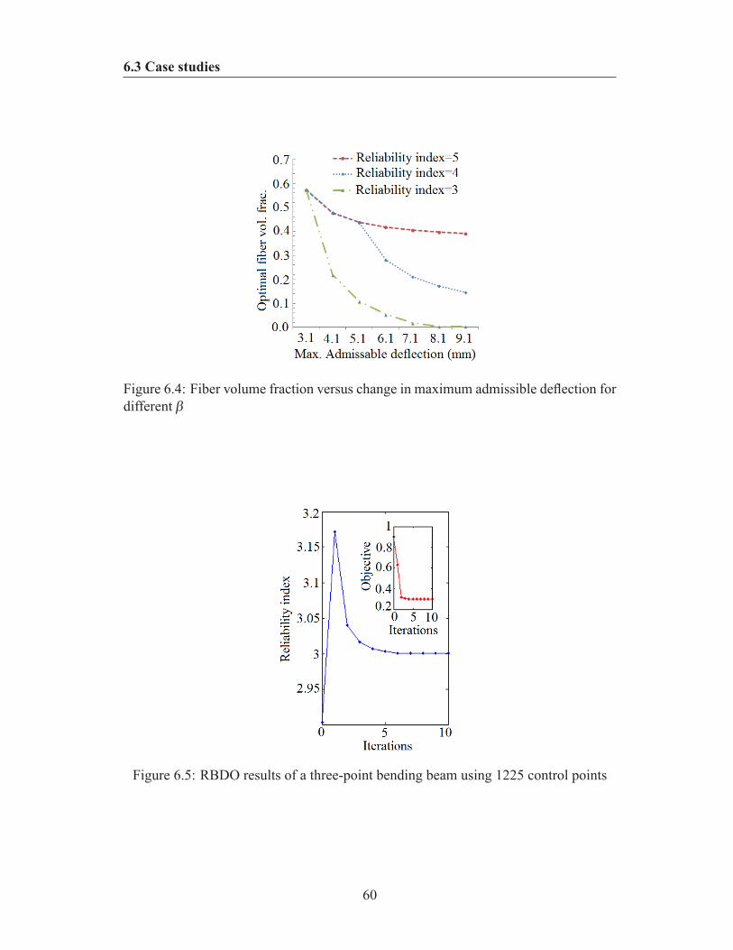
6.3 Case studies
Figure 6.4: Fiber volume fraction versus change in maximum admissible deflection fordifferent β
Figure 6.5: RBDO results of a three-point bending beam using 1225 control points
60
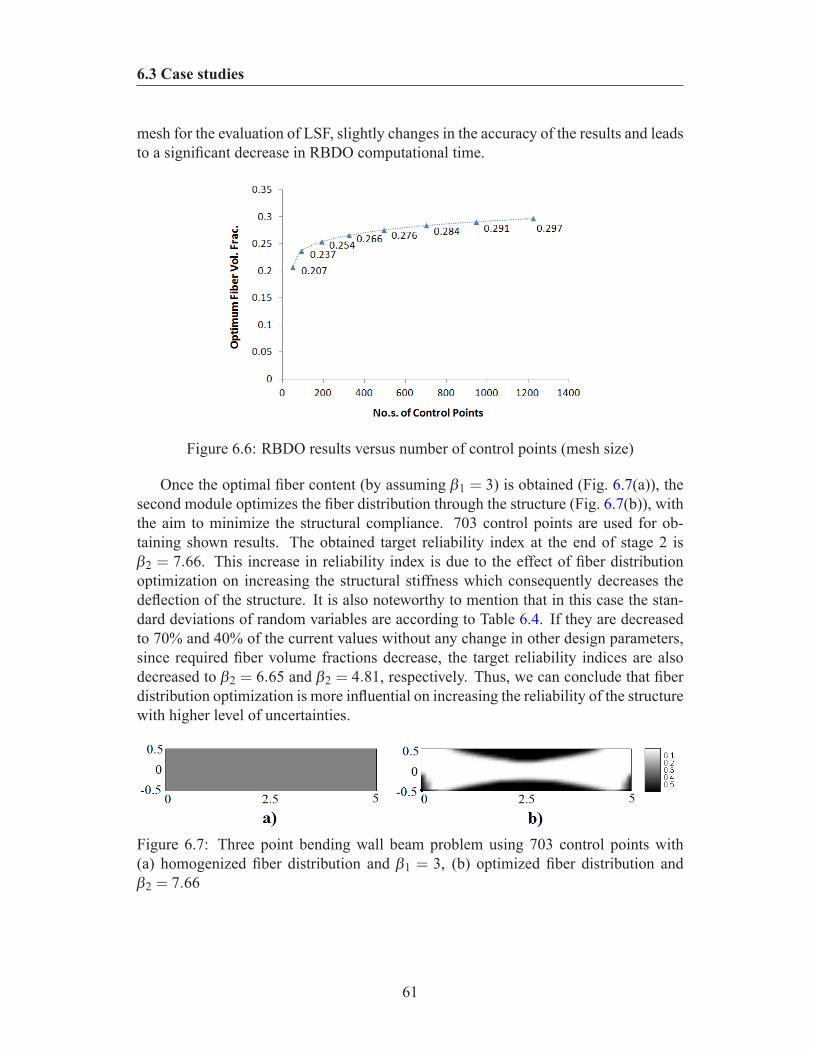
6.3 Case studies
mesh for the evaluation of LSF, slightly changes in the accuracy of the results and leadsto a significant decrease in RBDO computational time.
Figure 6.6: RBDO results versus number of control points (mesh size)
Once the optimal fiber content (by assuming β1 = 3) is obtained (Fig. 6.7(a)), thesecond module optimizes the fiber distribution through the structure (Fig. 6.7(b)), withthe aim to minimize the structural compliance. 703 control points are used for ob-taining shown results. The obtained target reliability index at the end of stage 2 isβ2 = 7.66. This increase in reliability index is due to the effect of fiber distributionoptimization on increasing the structural stiffness which consequently decreases thedeflection of the structure. It is also noteworthy to mention that in this case the stan-dard deviations of random variables are according to Table 6.4. If they are decreasedto 70% and 40% of the current values without any change in other design parameters,since required fiber volume fractions decrease, the target reliability indices are alsodecreased to β2 = 6.65 and β2 = 4.81, respectively. Thus, we can conclude that fiberdistribution optimization is more influential on increasing the reliability of the structurewith higher level of uncertainties.
Figure 6.7: Three point bending wall beam problem using 703 control points with(a) homogenized fiber distribution and β1 = 3, (b) optimized fiber distribution andβ2 = 7.66
61
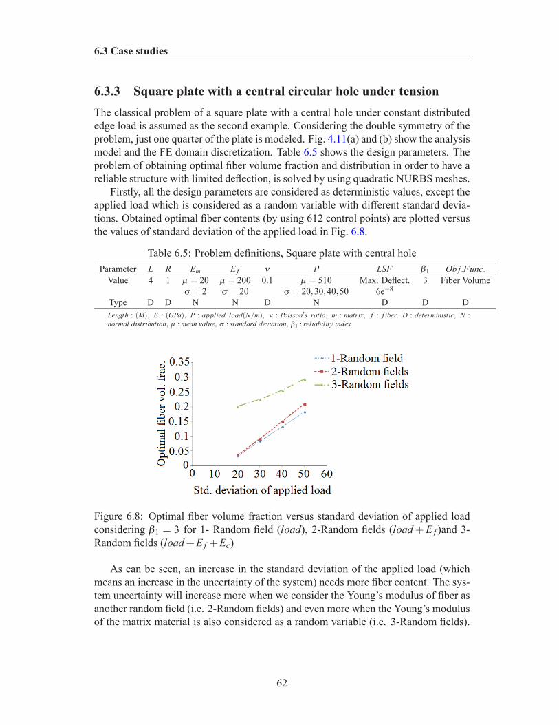
6.3 Case studies
6.3.3 Square plate with a central circular hole under tensionThe classical problem of a square plate with a central hole under constant distributededge load is assumed as the second example. Considering the double symmetry of theproblem, just one quarter of the plate is modeled. Fig. 4.11(a) and (b) show the analysismodel and the FE domain discretization. Table 6.5 shows the design parameters. Theproblem of obtaining optimal fiber volume fraction and distribution in order to have areliable structure with limited deflection, is solved by using quadratic NURBS meshes.
Firstly, all the design parameters are considered as deterministic values, except theapplied load which is considered as a random variable with different standard devia-tions. Obtained optimal fiber contents (by using 612 control points) are plotted versusthe values of standard deviation of the applied load in Fig. 6.8.
Table 6.5: Problem definitions, Square plate with central holeParameter L R Em E f ν P LSF β1 Ob j.Func.
Value 4 1 µ = 20 µ = 200 0.1 µ = 510 Max. Deflect. 3 Fiber Volumeσ = 2 σ = 20 σ = 20,30,40,50 6e−8
Type D D N N D N D D DLength : (M), E : (GPa), P : applied load(N/m), ν : Poisson′s ratio, m : matrix, f : f iber, D : deterministic, N :normal distribution, µ : mean value, σ : standard deviation, β1 : reliability index
Figure 6.8: Optimal fiber volume fraction versus standard deviation of applied loadconsidering β1 = 3 for 1- Random field (load), 2-Random fields (load +E f )and 3-Random fields (load +E f +Ec)
As can be seen, an increase in the standard deviation of the applied load (whichmeans an increase in the uncertainty of the system) needs more fiber content. The sys-tem uncertainty will increase more when we consider the Young’s modulus of fiber asanother random field (i.e. 2-Random fields) and even more when the Young’s modulusof the matrix material is also considered as a random variable (i.e. 3-Random fields).
62
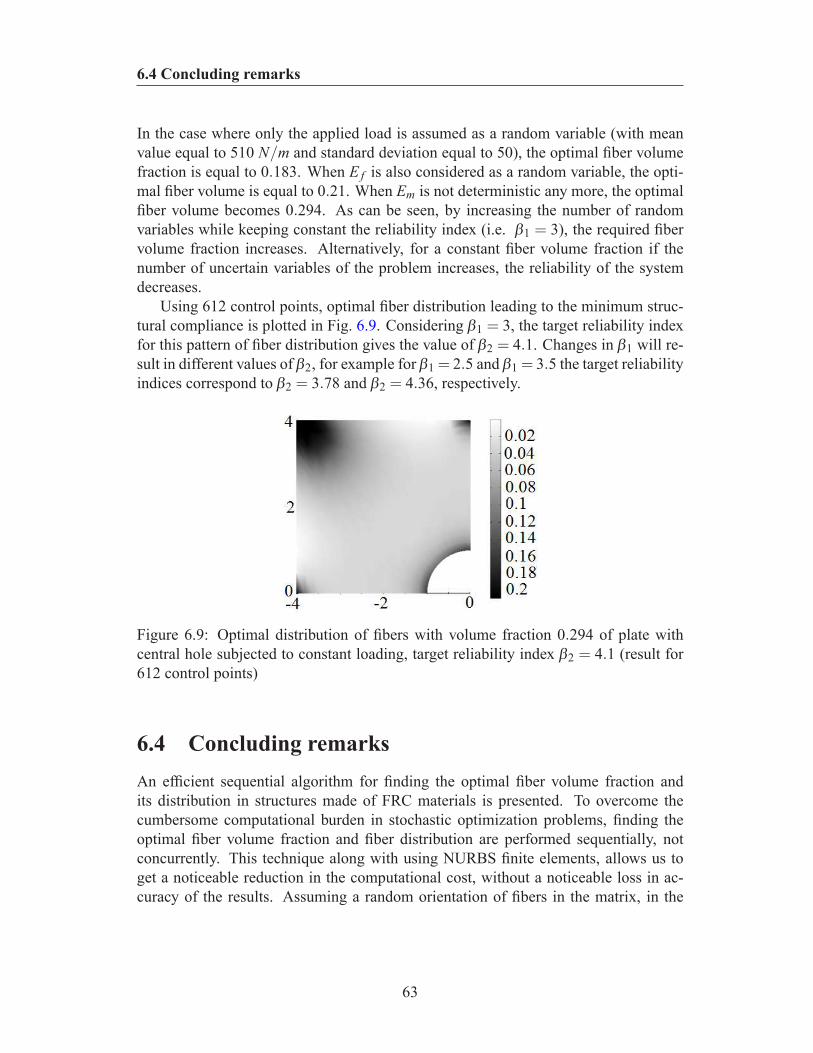
6.4 Concluding remarks
In the case where only the applied load is assumed as a random variable (with meanvalue equal to 510 N/m and standard deviation equal to 50), the optimal fiber volumefraction is equal to 0.183. When E f is also considered as a random variable, the opti-mal fiber volume is equal to 0.21. When Em is not deterministic any more, the optimalfiber volume becomes 0.294. As can be seen, by increasing the number of randomvariables while keeping constant the reliability index (i.e. β1 = 3), the required fibervolume fraction increases. Alternatively, for a constant fiber volume fraction if thenumber of uncertain variables of the problem increases, the reliability of the systemdecreases.
Using 612 control points, optimal fiber distribution leading to the minimum struc-tural compliance is plotted in Fig. 6.9. Considering β1 = 3, the target reliability indexfor this pattern of fiber distribution gives the value of β2 = 4.1. Changes in β1 will re-sult in different values of β2, for example for β1 = 2.5 and β1 = 3.5 the target reliabilityindices correspond to β2 = 3.78 and β2 = 4.36, respectively.
Figure 6.9: Optimal distribution of fibers with volume fraction 0.294 of plate withcentral hole subjected to constant loading, target reliability index β2 = 4.1 (result for612 control points)
6.4 Concluding remarksAn efficient sequential algorithm for finding the optimal fiber volume fraction andits distribution in structures made of FRC materials is presented. To overcome thecumbersome computational burden in stochastic optimization problems, finding theoptimal fiber volume fraction and fiber distribution are performed sequentially, notconcurrently. This technique along with using NURBS finite elements, allows us toget a noticeable reduction in the computational cost, without a noticeable loss in ac-curacy of the results. Assuming a random orientation of fibers in the matrix, in the
63
6.4 Concluding remarks
first optimization module (i.e. finding the optimal fiber volume fraction) uncertaintiesin the parameters (such as constituent’s materials and loading) are fully addressed andLSF is evaluated by using First Order Reliability Method (FORM). In the second mod-ule (i.e. fiber distribution optimization) a NURBS surface which smoothly defines thefiber distribution pattern, is adopted. The presented numerical examples show as anincrease in model uncertainties gives rise to unreliability of the system. More specif-ically, either the rise in the number of uncertain fields in the problem or the increasein the standard deviation of random variables needs more fiber content. It can be alsoconcluded that when there is a higher level of uncertainties in design parameters, thefiber distribution optimization is more influential on increasing the reliability of thestructure.
64
Chapter 7
Application 1: Interfacial shear stressoptimization in sandwich beams
7.1 IntroductionSandwich beams are a special class of composite materials fabricated by attachingtwo thin but stiff face sheets to a lightweight thick core which experiences mostlyshear stresses. As a result of their high bending stiffness and high strength to weightratios, sandwich beams have numerous applications in the automotive, aerospace, ma-rine and construction industries [Manalo et al., 2009]. A comprehensive review andassessment of various theories for modeling sandwich composites are presented in [Huet al., 2008]. Core shearing and debonding between core and face sheets are two com-mon failure modes of these structures. Core shearing occurs when a sandwich beamis subjected to an excessive transverse shear force. Moreover, experimental evidenceshows that debonding failure is influenced by the existence of a crack at the imperfectinterface [Triantafillou & Gibson, 1989]. The excessive interfacial stresses betweenthe core and the face sheet can be considered as a main cause for this failure.
To decrease the stress concentration at the interface, Functionally Graded Materials(FGMs) with continuously varying composition have been developed [Jha et al., 2013].However, Fiber Reinforced Composite (FRP) materials are also widely used in the coreof sandwich beams. Available research on interfacial stresses optimization mainlyconcerns beams strengthened with FRP bonded plate. For instance, Krour et al., 2013and Lousdad et al., 2010 tried to minimize interfacial stresses of a concrete beamstrengthened with FRP plate, by finding optimal fiber orientation in the FRP plate andits end shape, respectively.
Motivated by the capabilities of the fiber distribution optimization algorithm forFRC structures which has been described in Chapter 4, the methodology is extendedto present an optimization package for sandwich beams minimizing any stress state
65
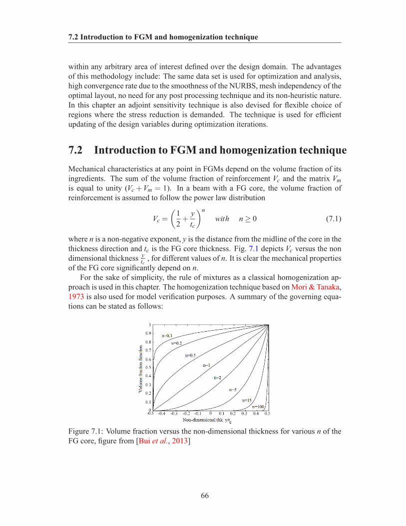
7.2 Introduction to FGM and homogenization technique
within any arbitrary area of interest defined over the design domain. The advantagesof this methodology include: The same data set is used for optimization and analysis,high convergence rate due to the smoothness of the NURBS, mesh independency of theoptimal layout, no need for any post processing technique and its non-heuristic nature.In this chapter an adjoint sensitivity technique is also devised for flexible choice ofregions where the stress reduction is demanded. The technique is used for efficientupdating of the design variables during optimization iterations.
7.2 Introduction to FGM and homogenization techniqueMechanical characteristics at any point in FGMs depend on the volume fraction of itsingredients. The sum of the volume fraction of reinforcement Vc and the matrix Vmis equal to unity (Vc +Vm = 1). In a beam with a FG core, the volume fraction ofreinforcement is assumed to follow the power law distribution
Vc =
(12+
ytc
)nwith n ≥ 0 (7.1)
where n is a non-negative exponent, y is the distance from the midline of the core in thethickness direction and tc is the FG core thickness. Fig. 7.1 depicts Vc versus the nondimensional thickness y
tc , for different values of n. It is clear the mechanical propertiesof the FG core significantly depend on n.
For the sake of simplicity, the rule of mixtures as a classical homogenization ap-proach is used in this chapter. The homogenization technique based on Mori & Tanaka,1973 is also used for model verification purposes. A summary of the governing equa-tions can be stated as follows:
Figure 7.1: Volume fraction versus the non-dimensional thickness for various n of theFG core, figure from [Bui et al., 2013]
66
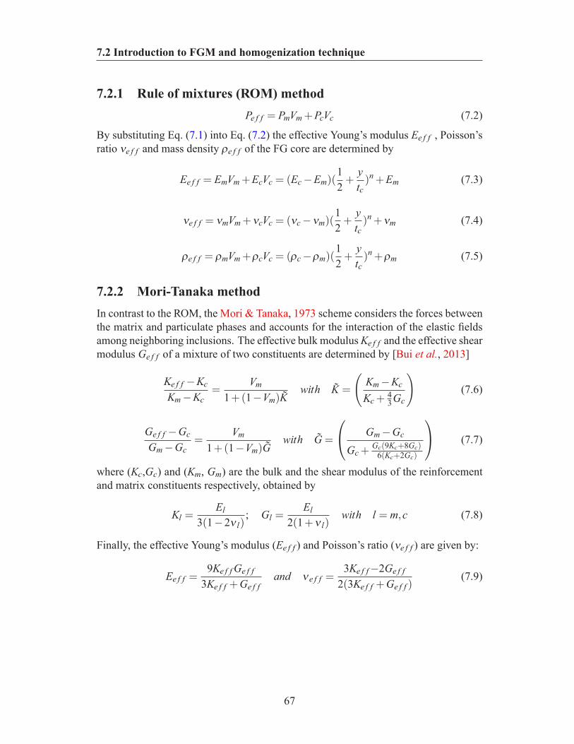
7.2 Introduction to FGM and homogenization technique
7.2.1 Rule of mixtures (ROM) methodPe f f = PmVm +PcVc (7.2)
By substituting Eq. (7.1) into Eq. (7.2) the effective Young’s modulus Ee f f , Poisson’sratio νe f f and mass density ρe f f of the FG core are determined by
Ee f f = EmVm +EcVc = (Ec −Em)(12+
ytc)n +Em (7.3)
νe f f = νmVm +νcVc = (νc −νm)(12+
ytc)n +νm (7.4)
ρe f f = ρmVm +ρcVc = (ρc −ρm)(12+
ytc)n +ρm (7.5)
7.2.2 Mori-Tanaka methodIn contrast to the ROM, the Mori & Tanaka, 1973 scheme considers the forces betweenthe matrix and particulate phases and accounts for the interaction of the elastic fieldsamong neighboring inclusions. The effective bulk modulus Ke f f and the effective shearmodulus Ge f f of a mixture of two constituents are determined by [Bui et al., 2013]
Ke f f −Kc
Km −Kc=
Vm
1+(1−Vm)Kwith K =
(Km −Kc
Kc +43Gc
)(7.6)
Ge f f −Gc
Gm −Gc=
Vm
1+(1−Vm)Gwith G =
Gm −Gc
Gc +Gc(9Kc+8Gc)
6(Kc+2Gc)
(7.7)
where (Kc,Gc) and (Km, Gm) are the bulk and the shear modulus of the reinforcementand matrix constituents respectively, obtained by
Kl =El
3(1−2ν l); Gl =
El2(1+ν l)
with l = m,c (7.8)
Finally, the effective Young’s modulus (Ee f f ) and Poisson’s ratio (νe f f ) are given by:
Ee f f =9Ke f f Ge f f
3Ke f f +Ge f fand νe f f =
3Ke f f−2Ge f f2(3Ke f f +Ge f f )
(7.9)
67
7.3 Material discontinuity
7.3 Material discontinuityIn a sandwich beam, material properties for the core and the face sheets are different,so the displacement solution at the interface of the core and the face sheets is only C0
continuous and the strain field (displacement gradient) is discontinuous across the ma-terial interface. It means there is discontinuity in gradient field. In classical C0 FEM,weak discontinuities can be automatically captured, if the material interface is locatedon an element boundary (conforming mesh). However, for problems with curved inter-faces, using conforming meshes may be cumbersome, especially when such interfacesevolve. Several advanced methods like the Extended Finite Element Method (XFEM)[Duddu et al., 2008 and Zhao et al., 2013], XIGA [Ghorashi et al., 2012 and Jia et al.,2014], Meshless [Zhuang et al., 2012 ; Rabczuk & Belytschko, 2004 ; Rabczuk et al.,2007 and Rabczuk & Belytschko, 2007] and the Numerical Manifold Method (NMM)[Cai et al., 2013] have been developed for capturing material discontinuity using nonconforming mesh. Recently Nguyen et al., 2014 proposed very simple approaches tohandle such discontinuities in IGA for composite delamination using knot insertion forcohesive interfaces.
In IGA, continuity across an interior element boundary directly depends on thepolynomial order and the multiplicity of the corresponding knot. Thus, knot insertioncan be used to tailor the continuity of the fields along element interface (see Fig. 7.2).Taking the knot vector in 1D as NNN =
ξ1,ξ2, ...,ξn+p+1
, where ξi is the ith knot, n is
the number of basis functions and p is the polynomial order, the basis functions acrossknot ξi are p−mi times continuously differentiable or Cp−mi continuous; where mi isthe multiplicity of knot ξi.
Fig. 7.2(a) and (b) present the physical and parametric spaces; Fig. 7.2(c) and (d)compare supports of the shape functions for interior (entirely inside the core or theface sheets) and interfacial elements. According to Fig. 7.2(c), control points corre-sponding to interior element No. 1 are 1,2,3,4,5,6,7,8,9 and for interior elementNo. 2 are 4,5,6,7,8,9,10,11,12. Two rows of control points (i.e. row 4,5,6 androw 7,8,9) are in common between these two elements. These shared control pointsproduce overlapping shape functions as illustrated in Fig. 7.2(c). In other words, theshape functions extend beyond the elements (C1 continuity). In contrary to the interiorelements, interfacial elements have at least one edge on the material interface. Twoof these elements (elements Nos. 3 and 4) are shown in Fig. 7.2(d). These two ele-ments have only one row of control points (i.e. row 27,28,29) in common due torepeated knot at the interface. This knot insertion imposes C0 continuity in the dis-placement field at the position of the material interface. As shown in Fig. 7.2(d), theshape functions of elements Nos. 3 and 4 do not overlap with each others.
In the present optimization methodology, control points which define the geometryof the model, contain the nodal volume fractions of the reinforcement as optimizationdesign variables. Note that this is an advantage due to the smoothness provided by the
68
7.3 Material discontinuity
Figure 7.2: Schematic illustration of C1 and C0 continuity of quadratic NURBS ele-ments, (a) physical mesh (b) parametric mesh (c) typical elements on single materialwithout interface with C1 continuity (d) typical elements on material interface with C0
continuity
69
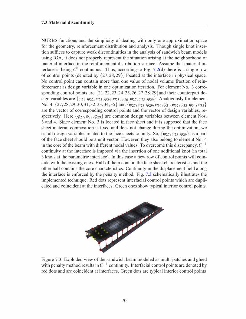
7.3 Material discontinuity
NURBS functions and the simplicity of dealing with only one approximation spacefor the geometry, reinforcement distribution and analysis. Though single knot inser-tion suffices to capture weak discontinuities in the analysis of sandwich beam modelsusing IGA, it does not properly represent the situation arising at the neighborhood ofmaterial interface in the reinforcement distribution surface. Assume that material in-terface is being C0 continuous. Thus, according to Fig. 7.2(d) there is a single rowof control points (denoted by 27,28,29) located at the interface in physical space.No control point can contain more than one value of nodal volume fraction of rein-forcement as design variable in one optimization iteration. For element No. 3 corre-sponding control points are 21,22,23,24,25,26,27,28,29and their counterpart de-sign variables are ϕ21,ϕ22,ϕ23,ϕ24,ϕ25,ϕ26,ϕ27,ϕ28,ϕ29. Analogously for elementNo. 4, 27,28,29,30,31,32,33,34,35 and ϕ27,ϕ28,ϕ29,ϕ30,ϕ31,ϕ32,ϕ33,ϕ34,ϕ35are the vector of corresponding control points and the vector of design variables, re-spectively. Here ϕ27,ϕ28,ϕ29 are common design variables between element Nos.3 and 4. Since element No. 3 is located in face sheet and it is supposed that the facesheet material composition is fixed and does not change during the optimization, weset all design variables related to the face sheets to unity. So, ϕ27,ϕ28,ϕ29 as a partof the face sheet should be a unit vector. However, they also belong to element No. 4in the core of the beam with different nodal values. To overcome this discrepancy, C−1
continuity at the interface is imposed via the insertion of one additional knot (in total3 knots at the parametric interface). In this case a new row of control points will coin-cide with the existing ones. Half of them contain the face sheet characteristics and theother half contains the core characteristics. Continuity in the displacement field alongthe interface is enforced by the penalty method. Fig. 7.3 schematically illustrates theimplemented technique. Red dots represent interfacial control points which are dupli-cated and coincident at the interfaces. Green ones show typical interior control points.
Figure 7.3: Exploded view of the sandwich beam modeled as multi-patches and gluedwith penalty method results in C−1 continuity. Interfacial control points are denoted byred dots and are coincident at interfaces. Green dots are typical interior control points
70
7.4 Overview of optimization methodology
7.4 Overview of optimization methodologyAs mentioned before, NURBS basis functions are used in this work not only for theanalysis but also to model the reinforcement distribution. In the present methodologythe nodal reinforcement volume fraction (ϕi, j) on control points are defined as designvariables and the reinforcement distribution (ηp) is approximated as NURBS surface.Every point in the parametric space is mapped to the physical space having two at-tributes, geometrical coordinates and reinforcement volume fraction value. Due to theintrinsic characteristics of NURBS (higher order continuity and compact support, see[Cottrell et al., 2009]), even coarse meshes yield smooth enough surfaces to clearlyrepresent the optimization results without needing any further image processing tech-niques.
The distribution function ηp(x,y), which indicates the amount of reinforcement atevery design point (x,y), is defined by Eq. (4.9) and used for obtaining the homoge-nized stiffness. Once the reinforcement volume fraction at each point is available, theequivalent mechanical characteristics of the domain are obtained through the rule ofmixtures
CCCeq (x,y) =(1−η p
)CCCm +η pCCCc (7.10)
where CCCeq; CCCm and CCCc are the homogenized, the matrix and the reinforcement elastictensors, respectively. Subsequently, CCCeq will be denoted by CCC. Since the core experi-ences mostly shear stresses, without loss of generality, the average value of the shearstresses within the area of interest is considered as the objective function. Other stresscomponents (i.e. bending and peeling) can be also taken into account in the same man-ner. For the plane stress assumption, the stress in a vector form (σσσ =
σxx,σyy,σxy
)
is given byσσσ = TuTuTu =CQuCQuCQu (7.11)
and alsoσσσ xy = tttxyuuu =CCCxyQuQuQu (7.12)
where TTT is the stress matrix of the element, (.)xy is the related row of (.) correspondingto the xy direction and QQQ is the matrix containing the derivatives of the shape functions.Thus, the objective function (J(uuu(ϕϕϕ),ϕϕϕ)) can be written in the following form
J(uuu(ϕϕϕ),ϕϕϕ) =1
|Ω1|
∫
Ω1σxy dΩ1 (7.13)
whereΩ1 is the area of interest over which the objective function is supposed to be min-imized. The optimization problem can be summarized according to Eq. (4.12) whilethe Lagrangian objective function and derivatives are defined according to Eq. (4.13)and Eq. (4.14), respectively. Once again the optimality criteria (OC) based optimiza-tion [Zhou & Rozvany, 1991] is implemented to numerically solve Eq. (4.14). Thedesign variables are updated by a sensitivity analysis as presented in following section.
71
7.4 Overview of optimization methodology
7.4.1 Adjoint sensitivity analysisIn gradient-based methods, to solve Eq. (4.14), one should differentiate the objectiveand constraint functions with respect to the design variables. The procedure to obtainthese derivatives is called sensitivity analysis. Generally, there are two main groupsof methods for sensitivity analysis: numerical methods (e.g. finite difference) whichare approximate; and analytical methods (including direct and adjoint methods) whichare exact. According to [Bendsoe & Sigmund, 2003] the most efficient method forcalculating derivatives involved in Eq. (4.14) is the adjoint method since there is a largenumber of design variables but few functions (here two, including objective functionand design constraint). Recalling Eq. (4.14), the chain-rule is used to calculate thesensitivity of J(uuu(ϕϕϕ),ϕϕϕ) with respect to ϕϕϕ
dJdϕϕϕ
=∂J∂uuu
∂uuu∂ϕϕϕ
+∂J∂ϕϕϕ
(7.14)
From force equilibrium (F=KuKuKu− fff = 000) we have
dFdϕϕϕ
=
(∂F∂uuu
)T ∂uuu∂ϕϕϕ
+∂F∂ϕϕϕ
= 0 (7.15)
∂uuu∂ϕϕϕ
=−
(∂F∂uuu
)−T ∂F∂ϕϕϕ
(7.16)
where (.)T denotes transpose of (.). Substitution of Eq. (7.16) in Eq. (7.14) yields to
dJdϕϕϕ
=−∂J∂uuu
[(∂F∂uuu
)−T ∂F∂ϕϕϕ
]+∂J∂ϕϕϕ
(7.17)
Introducing
λλλ =−∂J∂uuu
(∂F∂uuu
)−T(7.18)
and knowing that ∂F∂uuu =KKK, we can write
KλKλKλ =−∂J∂uuu
(7.19)
Eventually Eq. (7.14) can be written in the form
dJdϕϕϕ
= (λλλ )T ∂F∂ϕϕϕ
+∂J∂ϕϕϕ
(7.20)
72
7.5 Case studies
The second terms of Eq. (7.20) are obtained as follows
∂J∂ϕϕϕ
=1
|Ω1|
∫
Ω1
∂CCCxy∂ϕϕϕ
QQQuuu dΩ1 (7.21)
with∂CCCxy∂ϕϕϕ
=−∂η p∂ϕϕϕ
CCCmxy +∂η p∂ϕϕϕ
CCCcxy (7.22)
CCCmxy and CCCcxy in right hand side of Eq. (7.22) are related rows of CCCm and CCCc corre-sponding to the shear (xy) component. Considering Eq. (4.9), one can write
∂η p∂ϕ i, j
= Rp,qi, j (ξ ,η) (7.23)
to complete Eq. (7.20), ∂J∂uuu and ∂F
∂ϕϕϕ are needed
∂J∂uuu
=1
|Ω1|
∫
Ω1CCCxyQQQ dΩ1 (7.24)
and∂F∂ϕϕϕ
=∫
Ω
∂KKK∂ϕϕϕ
uuu dΩ (7.25)
where∂KKK∂ϕϕϕ
=∫
ΩQQQT ∂CCCeq
∂ϕϕϕQQQ dΩ (7.26)
Finally, the term dV fdϕϕϕ can be written as
dV fdϕϕϕ
=∂V f∂ϕϕϕ
=∫
Ω
∂η p∂ϕϕϕ
dΩ (7.27)
where ∂ηp∂ϕϕϕ can be obtained from Eq. (7.23).
7.5 Case studiesIn this section, the NURBS-based finite element model is verified by performing bothstatic and dynamic benchmark problems. Afterwards the performance of the optimiza-tion algorithm is studied.
73
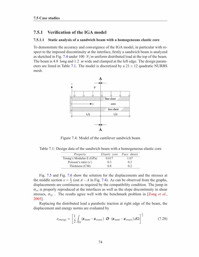
7.5 Case studies
7.5.1 Verification of the IGA model7.5.1.1 Static analysis of a sandwich beam with a homogeneous elastic core
To demonstrate the accuracy and convergence of the IGA model, in particular with re-spect to the imposed discontinuity at the interface, firstly a sandwich beam is analyzedas sketched in Fig. 7.4 under 100 N/m uniform distributed load at the top of the beam.The beam is 4.8 long and 1.2 m wide and clamped at the left edge. The design param-eters are listed in Table 7.1. The model is discretized by a 21×12 quadratic NURBSmesh.
Figure 7.4: Model of the cantilever sandwich beam
Table 7.1: Design data of the sandwich beam with a homogeneous elastic coreProperty Elastic core Face sheets
Young’s Modulus E (GPa) 0.617 1.67Poisson’s ratio (ν) 0.3 0.3Thickness (CM) 0.8 0.2
Fig. 7.5 and Fig. 7.6 show the solution for the displacements and the stresses atthe middle section x = L
2 (cut A−A in Fig. 7.4). As can be observed from the graphs,displacements are continuous as required by the compatibility condition. The jump inσxx is properly reproduced at the interfaces as well as the slope discontinuity in shearstresses, σxy . The results agree well with the benchmark problem in [Zong et al.,2005].
Replacing the distributed load a parabolic traction at right edge of the beam, thedisplacement and energy norms are evaluated by
eenergy =
[12
∫
Ω(εεεnum −εεεexact) ·DDD · (εεεnum −εεεexact)dΩ
] 12
(7.28)
74
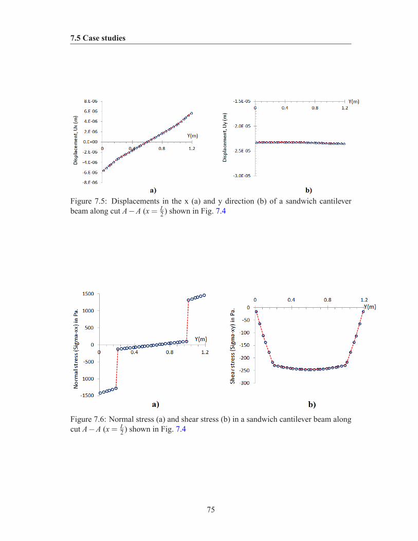
7.5 Case studies
Figure 7.5: Displacements in the x (a) and y direction (b) of a sandwich cantileverbeam along cut A−A (x = L
2 ) shown in Fig. 7.4
Figure 7.6: Normal stress (a) and shear stress (b) in a sandwich cantilever beam alongcut A−A (x = L
2 ) shown in Fig. 7.4
75
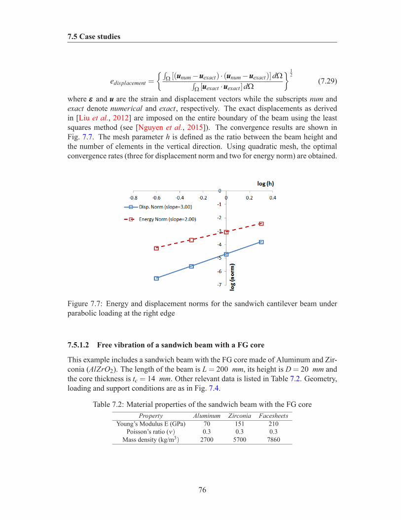
7.5 Case studies
edisplacement =
∫Ω [(uuunum −uuuexact) · (uuunum −uuuexact)]dΩ∫
Ω [uuuexact ·uuuexact ]dΩ
12
(7.29)
where εεε and uuu are the strain and displacement vectors while the subscripts num andexact denote numerical and exact, respectively. The exact displacements as derivedin [Liu et al., 2012] are imposed on the entire boundary of the beam using the leastsquares method (see [Nguyen et al., 2015]). The convergence results are shown inFig. 7.7. The mesh parameter h is defined as the ratio between the beam height andthe number of elements in the vertical direction. Using quadratic mesh, the optimalconvergence rates (three for displacement norm and two for energy norm) are obtained.
Figure 7.7: Energy and displacement norms for the sandwich cantilever beam underparabolic loading at the right edge
7.5.1.2 Free vibration of a sandwich beam with a FG core
This example includes a sandwich beam with the FG core made of Aluminum and Zir-conia (AlZrO2). The length of the beam is L = 200 mm, its height is D = 20 mm andthe core thickness is tc = 14 mm. Other relevant data is listed in Table 7.2. Geometry,loading and support conditions are as in Fig. 7.4.
Table 7.2: Material properties of the sandwich beam with the FG coreProperty Aluminum Zirconia Facesheets
Young’s Modulus E (GPa) 70 151 210Poisson’s ratio (ν) 0.3 0.3 0.3
Mass density (kg/m3) 2700 5700 7860
76
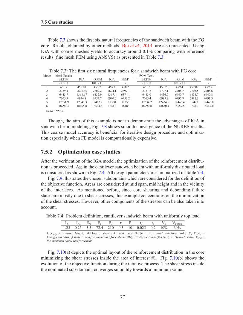
7.5 Case studies
Table 7.3 shows the first six natural frequencies of the sandwich beam with the FGcore. Results obtained by other methods [Bui et al., 2013] are also presented. UsingIGA with coarse meshes yields to accuracy around 0.1% comparing with referenceresults (fine mesh FEM using ANSYS) as presented in Table 7.3.
Table 7.3: The first six natural frequencies for a sandwich beam with FG coreMode Mori-Tanaka ROM Tech.
t-RPIM IGA t-RPIM IGA FEM∗ t-RPIM IGA t-RPIM IGA FEM∗
21 ×11 101 ×11 - 21 ×11 101 ×11 -1 461.7 458.01 459.2 457.8 458.2 461.5 459.28 459.4 459.02 459.52 2729.4 2695.65 2709.2 2694.1 2697.1 2727.8 2707.1 2708.7 2705.5 2708.63 6443.7 6368.67 6432.9 6367.4 6374.1 6443.0 6436.0 6440.7 6434.7 6440.84 7105.9 6944.8 6954.7 6940.0 6950.2 7065.4 6985.8 6995.8 6981.1 6991.35 12651.9 12341.3 12462.2 12330 12353 12634.2 12434.5 12446.4 12423 12446.06 18999.3 18465.8 18594.6 18441 18483 18990.8 18630.4 18659.5 18606 18647.0∗with ANSY S
Though, the aim of this example is not to demonstrate the advantages of IGA insandwich beam modeling, Fig. 7.8 shows smooth convergence of the NURBS results.This coarse model accuracy is beneficial for iterative design procedure and optimiza-tion especially when FE model is computationally expensive.
7.5.2 Optimization case studiesAfter the verification of the IGA model, the optimization of the reinforcement distribu-tion is proceeded. Again the cantilever sandwich beam with uniformly distributed loadis considered as shown in Fig. 7.4. All design parameters are summarized in Table 7.4.
Fig. 7.9 illustrates the chosen subdomains which are considered for the definition ofthe objective function. Areas are considered at mid span, mid height and in the vicinityof the interfaces. As mentioned before, since core shearing and debonding failurestates are mostly due to shear stresses, this example concentrates on the minimizationof the shear stresses. However, other components of the stresses can be also taken intoaccount.
Table 7.4: Problem definition, cantilever sandwich beam with uniformly top loadLx Ly Em Ec E f ν P t f tc Vc Vcmax
1.25 0.25 3.5 72.4 210 0.3 10 0.025 0.2 10% 60%Lx,Ly, t f , tc : beam length, thickness, f ace thk. and core thk.(m); V c : total rein f orc. vol., Em,Ec,E f :Young′s modulus o f matrix, rein f orcement and f ace sheet(GPa), P : Applied load (KN/m) ; ν : Poisson′s ratio, Vcmax :the maximum nodal rein f orcement
Fig. 7.10(a) depicts the optimal layout of the reinforcement distribution in the coreminimizing the shear stresses inside the area of interest #1. Fig. 7.10(b) shows theevolution of the objective function during the iterative process. The shear stress insidethe nominated sub-domain, converges smoothly towards a minimum value.
77
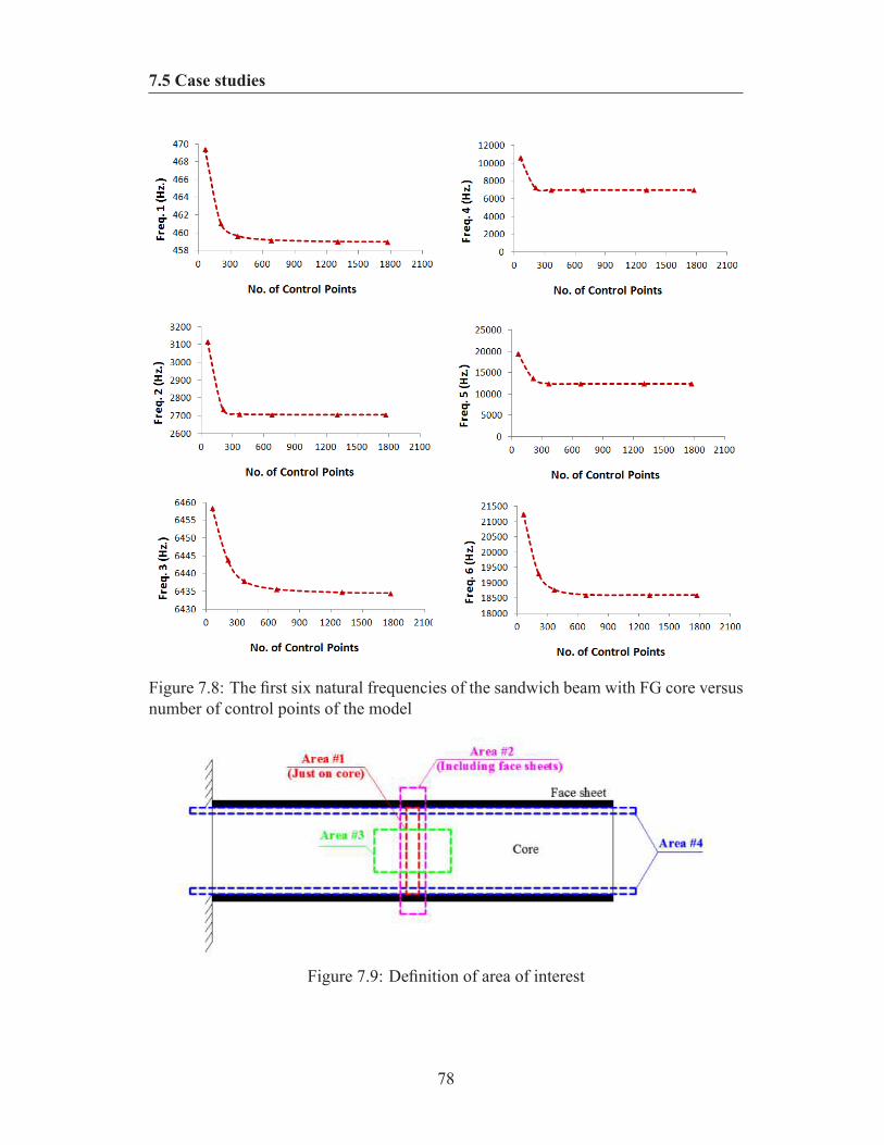
7.5 Case studies
Figure 7.8: The first six natural frequencies of the sandwich beam with FG core versusnumber of control points of the model
Figure 7.9: Definition of area of interest
78
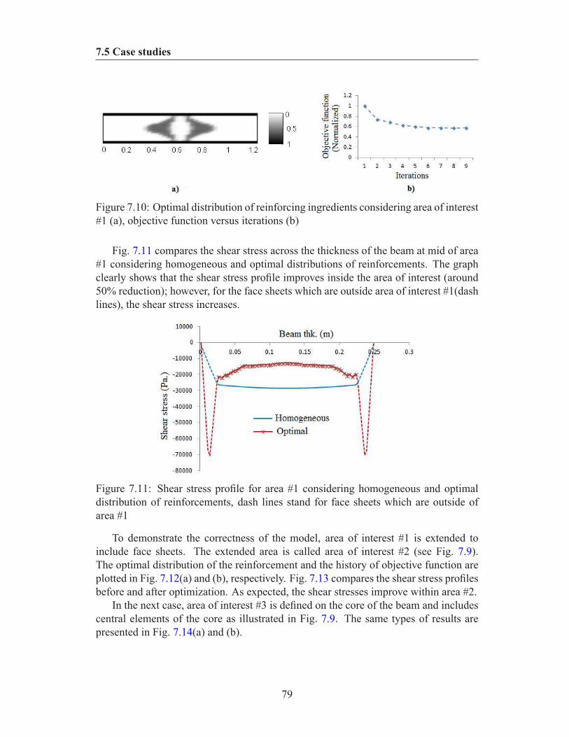
7.5 Case studies
Figure 7.10: Optimal distribution of reinforcing ingredients considering area of interest#1 (a), objective function versus iterations (b)
Fig. 7.11 compares the shear stress across the thickness of the beam at mid of area#1 considering homogeneous and optimal distributions of reinforcements. The graphclearly shows that the shear stress profile improves inside the area of interest (around50% reduction); however, for the face sheets which are outside area of interest #1(dashlines), the shear stress increases.
Figure 7.11: Shear stress profile for area #1 considering homogeneous and optimaldistribution of reinforcements, dash lines stand for face sheets which are outside ofarea #1
To demonstrate the correctness of the model, area of interest #1 is extended toinclude face sheets. The extended area is called area of interest #2 (see Fig. 7.9).The optimal distribution of the reinforcement and the history of objective function areplotted in Fig. 7.12(a) and (b), respectively. Fig. 7.13 compares the shear stress profilesbefore and after optimization. As expected, the shear stresses improve within area #2.
In the next case, area of interest #3 is defined on the core of the beam and includescentral elements of the core as illustrated in Fig. 7.9. The same types of results arepresented in Fig. 7.14(a) and (b).
79
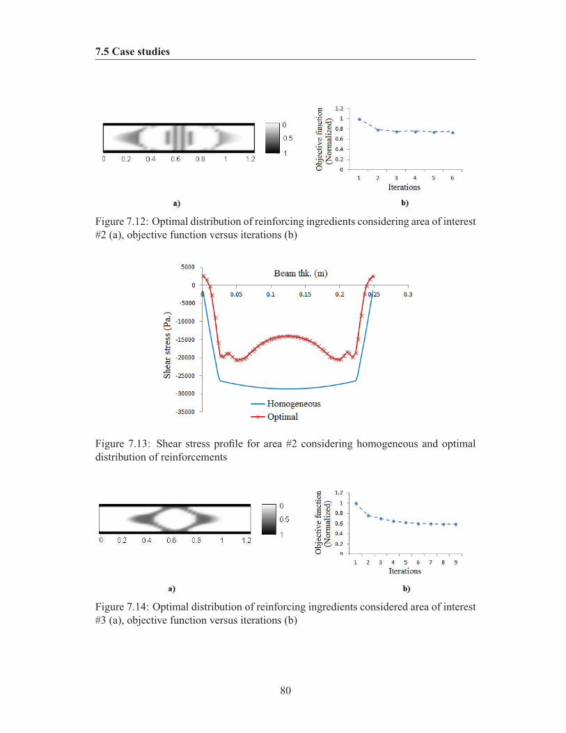
7.5 Case studies
Figure 7.12: Optimal distribution of reinforcing ingredients considering area of interest#2 (a), objective function versus iterations (b)
Figure 7.13: Shear stress profile for area #2 considering homogeneous and optimaldistribution of reinforcements
Figure 7.14: Optimal distribution of reinforcing ingredients considered area of interest#3 (a), objective function versus iterations (b)
80
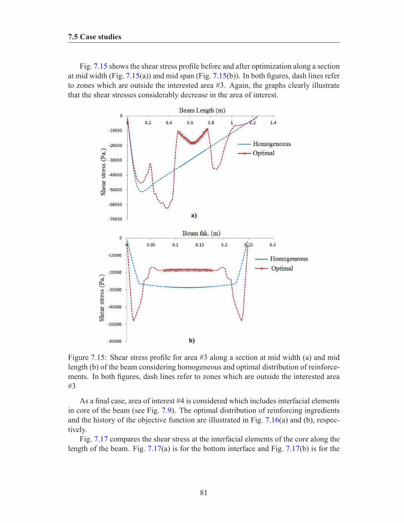
7.5 Case studies
Fig. 7.15 shows the shear stress profile before and after optimization along a sectionat mid width (Fig. 7.15(a)) and mid span (Fig. 7.15(b)). In both figures, dash lines referto zones which are outside the interested area #3. Again, the graphs clearly illustratethat the shear stresses considerably decrease in the area of interest.
Figure 7.15: Shear stress profile for area #3 along a section at mid width (a) and midlength (b) of the beam considering homogeneous and optimal distribution of reinforce-ments. In both figures, dash lines refer to zones which are outside the interested area#3
As a final case, area of interest #4 is considered which includes interfacial elementsin core of the beam (see Fig. 7.9). The optimal distribution of reinforcing ingredientsand the history of the objective function are illustrated in Fig. 7.16(a) and (b), respec-tively.
Fig. 7.17 compares the shear stress at the interfacial elements of the core along thelength of the beam. Fig. 7.17(a) is for the bottom interface and Fig. 7.17(b) is for the
81
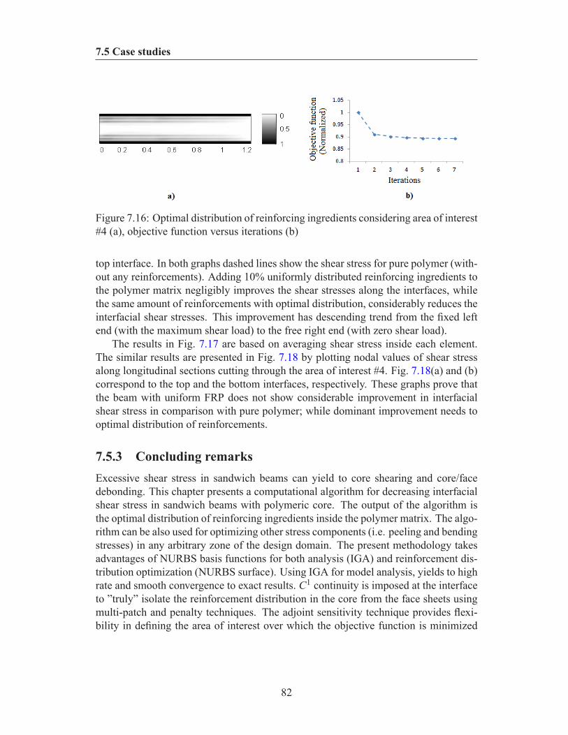
7.5 Case studies
Figure 7.16: Optimal distribution of reinforcing ingredients considering area of interest#4 (a), objective function versus iterations (b)
top interface. In both graphs dashed lines show the shear stress for pure polymer (with-out any reinforcements). Adding 10% uniformly distributed reinforcing ingredients tothe polymer matrix negligibly improves the shear stresses along the interfaces, whilethe same amount of reinforcements with optimal distribution, considerably reduces theinterfacial shear stresses. This improvement has descending trend from the fixed leftend (with the maximum shear load) to the free right end (with zero shear load).
The results in Fig. 7.17 are based on averaging shear stress inside each element.The similar results are presented in Fig. 7.18 by plotting nodal values of shear stressalong longitudinal sections cutting through the area of interest #4. Fig. 7.18(a) and (b)correspond to the top and the bottom interfaces, respectively. These graphs prove thatthe beam with uniform FRP does not show considerable improvement in interfacialshear stress in comparison with pure polymer; while dominant improvement needs tooptimal distribution of reinforcements.
7.5.3 Concluding remarksExcessive shear stress in sandwich beams can yield to core shearing and core/facedebonding. This chapter presents a computational algorithm for decreasing interfacialshear stress in sandwich beams with polymeric core. The output of the algorithm isthe optimal distribution of reinforcing ingredients inside the polymer matrix. The algo-rithm can be also used for optimizing other stress components (i.e. peeling and bendingstresses) in any arbitrary zone of the design domain. The present methodology takesadvantages of NURBS basis functions for both analysis (IGA) and reinforcement dis-tribution optimization (NURBS surface). Using IGA for model analysis, yields to highrate and smooth convergence to exact results. C1 continuity is imposed at the interfaceto ”truly” isolate the reinforcement distribution in the core from the face sheets usingmulti-patch and penalty techniques. The adjoint sensitivity technique provides flexi-bility in defining the area of interest over which the objective function is minimized
82
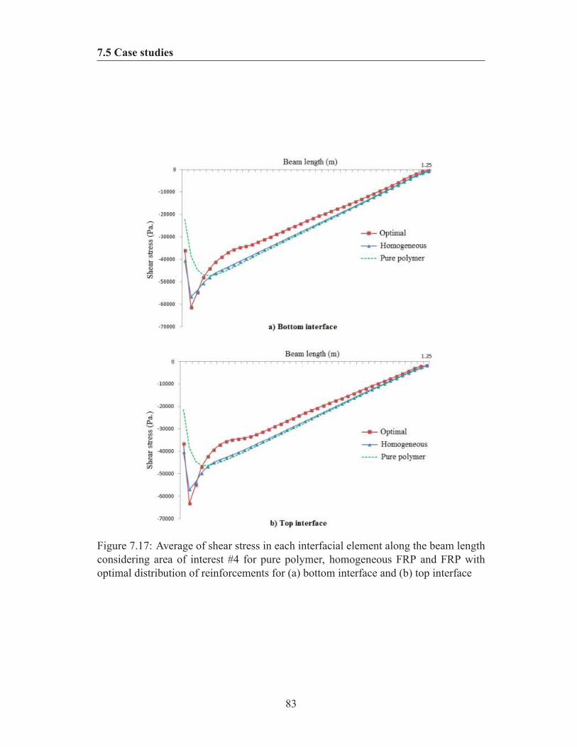
7.5 Case studies
Figure 7.17: Average of shear stress in each interfacial element along the beam lengthconsidering area of interest #4 for pure polymer, homogeneous FRP and FRP withoptimal distribution of reinforcements for (a) bottom interface and (b) top interface
83
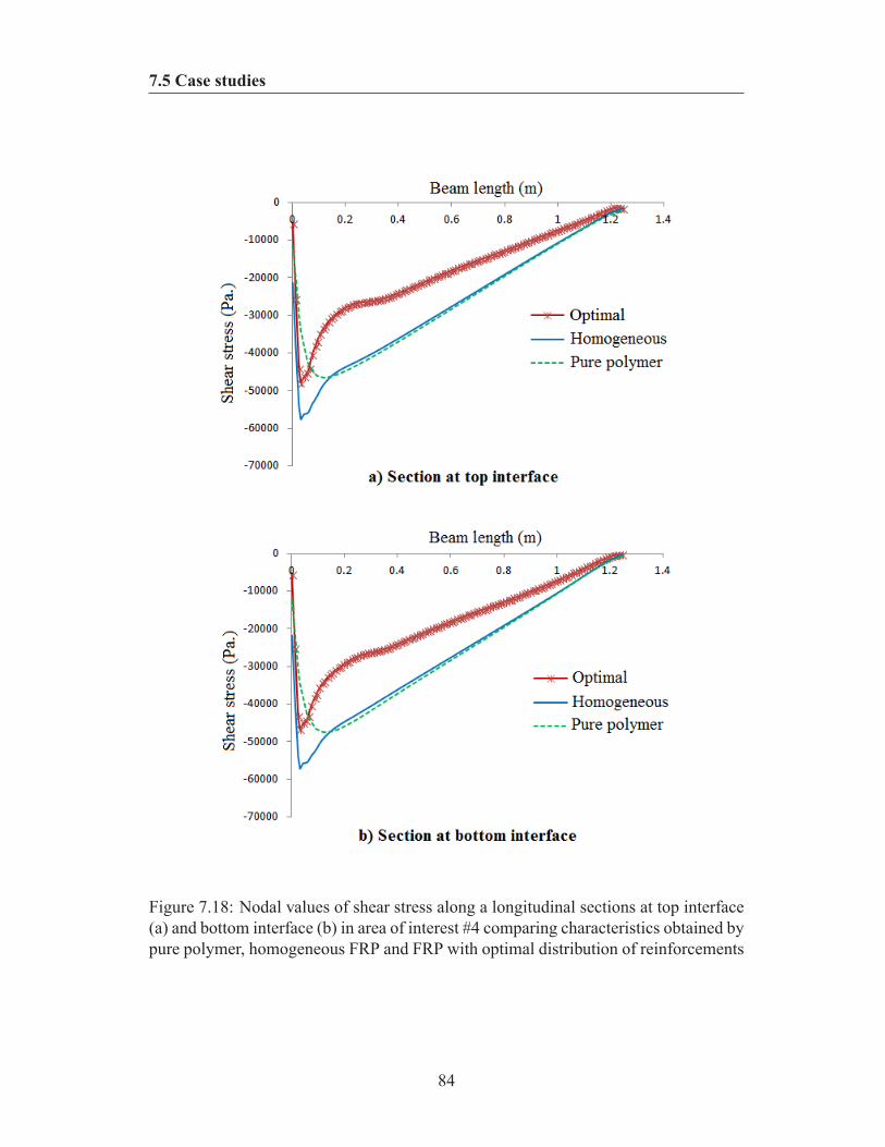
7.5 Case studies
Figure 7.18: Nodal values of shear stress along a longitudinal sections at top interface(a) and bottom interface (b) in area of interest #4 comparing characteristics obtained bypure polymer, homogeneous FRP and FRP with optimal distribution of reinforcements
84

7.5 Case studies
and also for efficient updating of the design variables through optimization iterations.Comparing the results of the case study illustrates that adding reinforcements homo-geneously into polymers will slightly improve the interfacial shear stress but that con-siderable improvements are observed when the distribution of the reinforcement in thecore is optimized.
85
Chapter 8
Application 2: Probabilisticmulticonstraints optimization ofcooling channels in ceramic matrixcomposites
8.1 IntroductionThe main disadvantage of monolithic ceramics is their low fracture toughness. Thus,carbon fibers are added to increase their damage tolerance while maintaining otheradvantages (for instance lower density and higher maximum operating temperaturecompared to metals or high erosion and corrosion resistance).
As a common reinforcing ingredient, Carbon fibers (C-fibers) degrade in an oxi-dizing atmosphere beyond 450 degrees Celsius [Krenkel, 2005]. Although multilayerprotection coatings hinder degradation to a degree, the coating process may itself resultin formation of interphasial cracks. Preventing high temperature zones in the compo-nent might be a better solution. Such a solution however calls for a multidisciplinaryapproach accounting for material selection, coating and internal cooling design.
This chapter presents a computational framework for an efficient and reliable in-ternal cooling network for a typical component made of Ceramic Matrix Compos-ite (CMC). Although some attempts to optimize internal cooling system of a mono-tonic metallic turbine blade exist, the currently known approaches are limited to usingheuristic optimization methods, particularly Genetic Algorithm (GA) which is compu-tationally expensive. For example, Dennis et al., 2003 used parallel genetic algorithmto optimize locations and discrete radii of a large number of small circular cross-sectioncoolant passages. Nagaiah & Geiger, 2014 used NSGA-II as a multiobjective evolu-tionary algorithm optimizing the rib design inside a 2D cooling channel of a gas tur-
86

8.2 Thermoelastic formulation
bine blade. In both works an external commercial finite element package is used forthe thermal analysis.
Regardless of the optimization technique, another major drawback of current meth-ods is their deterministic nature. Actual characteristics of a composite material (includ-ing CMC) involve many uncertainties. These emanate from a variety of sources suchas constituent material properties, manufacturing and process imperfections, loadingconditions and geometry (a classification is presented in chapter 5. Neglecting the roleof uncertainties in composite materials might result in either unsafe or unnecessaryconservative design. This chapter focuses not only on optimal but also on reliable de-sign of a typical internal cooling network within a CMC using a non-heuristic methodand accounting for uncertainties.
The double stage sequential optimization approach (see Chapter 6) is implemented.In the first stage, it is assumed that C-fibers are uniformly distributed in the ceramicmatrix. Then by using RBDO, the outputs of the first stage which are optimal capacitiesof the cooling channels, are exported into the next stage. In the second stage, theoptimizer takes these inputs and uses the adjoint sensitivity technique adopted for thecoupled elastic and thermal fields and eventually provides an optimal distribution ofthe C-fibers within the design domain in order to enhance the target reliability of thecomponent.
8.2 Thermoelastic formulationThe steady-state governing equation and boundary conditions for a temperature fieldin a 2D isotropic solid with domain Ω and boundary Γ are [Wu et al., 2009]
(ki jθ , j
),i +Q = 0 in Ω (8.1)
θ = θΓ on Γ1 Essential boundary (8.2)
−niki jθ , j = qΓ on Γ2 Heat f lux boundary (8.3)
−niki jθ , j = h(θ −θ∞) on Γ3 Convection boundary (8.4)
−niki jθ , j = 0 on Γ4 Adiabatic boundary (8.5)
where ki j, Q, and θ denote the thermal conductivity, internal uniform heat source andtemperature field, respectively; ni is component of the unit outward normal to theboundary, h is the heat convection coefficient, qΓ is the prescribed heat flux and θ∞
87

8.2 Thermoelastic formulation
is the temperature of the surrounding medium in convection process. The governingequation and boundary conditions for a linear elastic solid are given by
σ i j, j +bi = 0 in Ω (8.6)
ui = uΓ on Γu Essential boundary (8.7)
σ i jni = tΓ on Γt Heat f lux boundary (8.8)
where σ and b denote the stress and body force. uΓ and tΓ are the given displacementand traction on the essential and natural boundaries, respectively.
The heat and elastic problems are linked by the following stress, strain and thermalexpansion relation
σ i j = δ i jλLεkk +2µLε i j −δ i j(3λL +2µL)α∆θ (8.9)
where λL and µL are Lame constants, α is the thermal expansion coefficient and ∆θis the temperature change with respect to the reference temperature which is assumedzero here.
A weighted residual weak form of the boundary value problem (Eq. (8.1)- (8.5))can be written as a generalized functional I
I (θ) =∫
Ωw[(ki j θ , j),i +Q
]dΩ= 0 (8.10)
where w denotes the sufficiently differentiable test function. Differentiation by partsand using Green’s theorem, the functional I(θ) can be written as
I (θ) =∫
Ω
12
[kx1
(∂θ∂x1
)2+ kx2
(∂θ∂x2
)2]
dΩ−∫
ΩθQdΩ+
∫
Γ2θqΓdΓ+
∫
Γ3hθ(
12θ −θ∞
)dΓ= 0
(8.11)
considering δ as the variational operator, the Bubnov-Galerkin weak form for the heattransfer problem can be obtained as follows
∫
Ωδ (∇θθθ)TKKKc∇θθθdΩ−
∫
ΩδθθθT QdΩ+
∫
Γ2δθθθT qΓdΓ+
∫
Γ3δθθθT hθθθdΓ−
∫
Γ3δθθθT hθ∞dΓ= 0
(8.12)
The strains arising from boundary loadings and body forces induce only small tem-perature changes which can be ignored in the analysis. Thus, the semi-coupled theory
88
8.2 Thermoelastic formulation
of thermoelasticity is employed here. The heat governing equations are firstly solvedto obtain the temperature field. Then, the body forces induced by the temperature fieldare used along with the other applied forces to calculate the final response of the elasticbody. Using the Bubnov-Galerkin weak form∫
Ωδ (εεε (uuu)−εεεθ (uuu))TCCC (εεε (uuu)−εεεθ (uuu))dΩ−
∫
ΓtδuuuT tΓdΓ−
∫
ΩδuuuTbbbdΩ= 0 (8.13)
B-spline basis functions are selected as the test function w. They are also employedto approximate the displacement and temperature fields
u(x,y) =n
∑i=1
m
∑j=1
N p,qi, j (ξ ,η)ui, j =NNN uuu (8.14)
θ(x,y) =n
∑i=1
m
∑j=1
N p,qi, j (ξ ,η) θ i, j =NNNθθθ (8.15)
where uuu and θθθ denotes the vector of nodal displacements and temperatures, respec-tively. The strain-displacement and the heat flux-temperature gradient relationshipscan be written as:
εεε =BBBeuuu and ggg =BBBheatθθθ (8.16)
BBBe and BBBheat are the matrices containing the derivatives of the shape functions, NNN,corresponding to the elastic and thermal problems, respectively.
By substituting the B-spline approximation function into Eq. (8.12), the discretizedsystem of equations can be expressed in the following matrix form
KKKcθθθ = fff heat (8.17)
The local conduction matrix, KKKc, and the heat force vector, fff heat , are determinedaccording to
KKKc =∫
ΩBBBT
heat HHH BBBheatdΩ+∫
Γ3hNNNTNNNdΓ3 (8.18)
fff heat = fff Q + fff h + fff q (8.19)
wherefff Q =
∫
ΩNNNT QdΩ (8.20)
fff h =∫
Γ3NNNT hθ∞dΓ3 (8.21)
fff q =−∫
Γ2NNNT qΓdΓ2 (8.22)
89
8.2 Thermoelastic formulation
Superscript T is used in this chapter to denote transpose of a matrix; HHH is the heatconduction matrix. The first and the second integrals in Eq. (8.18) correspond to theheat conduction (in volume Ω) and the convection (on surface Γ3 ). The heat forcevector contains fff Q, fff h and fff q induced by the uniform heat source Q, the heat convec-tion and heat flux qΓ, respectively. Substituting the test function and its derivatives intoEq. (8.13) leads finally the discretized linear system of equations for the thermoelas-ticity problem in the following matrix form
KuKuKu = fff total (8.23)
The global stiffness matrix of the elastic problem, KKK, is obtained by
KKK =∫
ΩBBBe
TCCC BBBe dΩ (8.24)
whilefff total = fff m + fff θ (8.25)
where fff m is the force vector corresponding to mechanical loading
fff m =∫
ΓtNNNT tΓdΓ+
∫
ΩNNNT bdΩ (8.26)
The body forces induced by the temperature field, fff θ , are also calculated using thefollowing equation
fff θ =∫
ΩBBBe
TCCCεεεθdΩ (8.27)
where CCC is the elasticity matrix and εεεθ is the thermal strain matrix which for the caseof plane stress with an isotropic material is obtained by
εεεθ =
α∆θα∆θ
0
(8.28)
It is also noteworthy to declare that, in this work the cross section area of a typicalcooling channel is assumed much smaller than the area of the design domain. Such acooling source which exists within a small area only, may be idealized as a point heatsink. This point sink is modeled by simply including a node at the location of the pointsource in the discretized model [Logan, 2007]. In the two dimensional element, for atypical cooling source, Qi, located at x = x0 and y = y0 one can write
fff Qi =NNNT0 Qi (8.29)
where NNN0 is the vector of shape functions evaluated at x = x0 and y = y0.
90

8.3 Reliability based design
8.3 Reliability based design
8.3.1 Deterministic design versus reliability based designTraditional factor of safety would provide a safety margin to cover uncertainties inloads, material parameters and in the model. This factor is in principle deterministicbut its magnitude is usually obtained based on experience which may include stochasticdata. There are two major concerns related to this concept of safety: 1) conservatismand 2) inability to reflect differing degrees of control on design variables [Nikolaidiset al., 2005]. Both of these issues might lead to costly suboptimal designs.
New market demands along with shortcomings of traditional deterministic designapproaches led to the development of nondeterministic approaches. One approach usesprobability theory for capturing the uncertainties and measuring the reliability of thesystem. In probabilistic analysis, design variables and parameters are assumed to berandom variables with selected joint probability density functions (pdf).
8.3.2 Probabilistic multiconstraintsIn this chapter the probabilistic thermal and elastic design limit states are consideredas a series constraints. It means that violation of at least one constraint yields to theentire system failure. As is shown in Fig. 8.1, the failure region is the union of twofailure subsets corresponding to each limit state. In mathematical form the failuredomain D with two limit state functions gi(x) where i = 1,2 can be expressed as D =x|⋃
i gi(x)≤ 0.
Figure 8.1: Schematic illustration of the failure domain with two probabilistic designconstraints
The system failure probability can be obtained by Pf = 1−Φm(B,R) whereΦm(B,R)is the m-variant standard normal CDF with B= β1, ...,βm and R= ρKL ; ρKL =αkαT
1
91
8.4 Adopting the double sequential stages optimization methodology
where αk is the unit normal to the hyperplane obtained by FORM approximation[Nikolaidis et al., 2005]. The open source software FERUM 4.1 [Bourinet, 2010]has been extended to perform the reliability analysis for multiconstraints problems.
8.3.3 RBDORBDO deals with obtaining optimal design with low failure probability. A double-loop(nested) algorithm is employed where the outer loop finds the optimal values for thedesign variables and the inner loop performs the reliability analysis. Here, the RBDOis performed as the first stage of the optimization process. The first objective functionis minimizing the total required cooling capacity of the heat sinks. The probabilisticconstraints are defined on maximum deflection and maximum temperature of the com-ponent as the series constraints. Thus, the first stage of the optimization problem canbe summarized as follows
Minimize : C (QQQ) = ∑ni=0 Qi where n = number o f cooling channels
sub jected to :
Probabilistic Constraints :
Pf ,1 = Prob(θ allow −θmax < 0)≤ Pf
Pf ,2 = Prob(δ all −δmax < 0)≤ Pf
Deterministic Constraints : QLj ≤ Q j ≤ QU
j where j ∈ 1,2, . . . ,n
(8.30)
where θallow and δall are the maximum allowable temperature and deflection, respec-tively. These two parameters as well as the prescribed failure probabilities (i.e. P f )should be decided by the designer at the beginning of the optimization process. Q jdenotes the cooling capacity of the jth channel; θmax and δmax are the correspondingmaximum values obtained from the solution of the thermoelastic governing equationsdescribed in Section 8.2.
8.4 Adopting the double sequential stages optimizationmethodology
The optimization algorithm for this application includes two independent but sequen-tially linked stages. In the first stage, it is assumed that the C-fibers are uniformlydistributed in the matrix. According to Eq. (8.30), the total required cooling capacityof the channels is optimized through the RBDO approach. Mechanical (maximum de-flection) as well as thermal (maximum temperature) probabilistic design constraints areenforced. The deterministic design constraints also limit the capacities of the coolingchannels. Random variables include constituent material properties (Young’s modulus
92
8.4 Adopting the double sequential stages optimization methodology
and heat conduction coefficient for the both C-fibers and ceramic matrix), applied load,applied heat flux and film convection coefficient. The output of this stage is used asthe input for the second stage.
ϕi, j are the only design variables in the second optimization stage which are definedon the mesh control points. When the reinforcement volume fraction at each point isavailable (Eq. (4.9)), the equivalent properties are defined as follows
Meq (x,y) =(1−η p
)Mm +η pMc with M = E , k, α (8.31)
where, E, k and α denote the Young’s modulus, thermal conductivity and thermalexpansion coefficient, respectively. Subscripts eq, m and c represent homogenized,matrix and C-fibers respectively. For the sake of notation simplicity, Meq is denotedby M in the following. The multiobjective optimization problem is defined as theweighted sum of different normalized objective functions. The target (total) objectivefunction, J (uuu(ϕϕϕ) ,θθθ (ϕϕϕ) ,ϕϕϕ), consists of the structural compliance and the so called”thermal compliance” yielding
J (uuu(ϕϕϕ) ,θθθ (ϕϕϕ) ,ϕϕϕ) =W1S1
(12
∫
Ω(BBBeuuu)TCCC (BBBeuuu)dΩ
)+
W2S2
(12
∫
Ω(BBBheatθθθ)
THHH(BBBheatθθθ) dΩ) (8.32)
where ϕϕϕ denotes the vector containing all ϕ(i, j) and Ω is the entire design domain; Wiand Si denote the ith weight and scaling factor, respectively. The optimization problemin the second stage can then be summarized as follows
Minimize : J (uuu(ϕϕϕ) ,θθθ (ϕϕϕ) ,ϕϕϕ)Sub jected to :
V f =∫Ωη p dΩ=V f 0
F1 (θθθ(ϕϕϕ),ϕϕϕ) =KKKcθθθ − fff heat = 000F2 (uuu(ϕϕϕ),θθθ(ϕϕϕ),ϕϕϕ) =KuKuKu− fff m − fff θ = 000ϕ i, j −1 ≤ 0−ϕ i, j ≤ 0
(8.33)
where V f is the total C-fibers volume in each optimization iteration, V f 0 is an arbitraryinitial C-fibers volume which must be set at the beginning of the optimization process.
8.4.1 Adjoint sensitivity analysisBy using the chain-rule one can calculate the sensitivity of the objective function,J (uuu(ϕϕϕ) ,θθθ (ϕϕϕ) ,ϕϕϕ), with respect to ϕϕϕ
dJdϕϕϕ
=∂J∂uuu
∂uuu∂ϕϕϕ
+∂J∂θθθ
∂θθθ∂ϕϕϕ
+∂J∂ϕϕϕ
(8.34)
93
8.4 Adopting the double sequential stages optimization methodology
The last term of Eq. (8.34) is the explicit quantity and easy to calculate
∂J∂ϕϕϕ
=W1S1
(12
∫
Ω(BBBeuuu)T ∂CCC
∂ϕϕϕ(BBBeuuu) dΩ
)+
W2S2
(12
∫
Ω(BBBheatθθθ)
T ∂HHH∂ϕϕϕ
(BBBheatθθθ) dΩ) (8.35)
while
∂CCC∂ϕϕϕ
=−∂η p∂ϕϕϕ
(Em
1−ν2
)
1 ν 0ν 1 00 0
(1−ν2)
+
∂η p∂ϕϕϕ
(Ec
1−ν2
)
1 ν 0ν 1 00 0
(1−ν2)
(8.36)and
∂HHH∂ϕϕϕ
=−∂η p∂ϕϕϕ
[km 00 km
]+
∂η p∂ϕϕϕ
[kc 00 kc
](8.37)
Moreover∂η p∂ϕ i, j
= N p,qi, j (ξ ,η) (8.38)
The first and the second terms of Eq. (8.34) include implicit quantities (i.e. ∂uuu∂ϕϕϕ and
∂θθθ∂ϕϕϕ ) which are accomplished by using the heat conduction and linear elasticity forceequilibrium equations (see F1 and F2 in Eq. (8.33)) as adjoint equations.
By differentiating, we have(∂F1∂θθθ
)T ∂θθθ∂ϕϕϕ
+∂F1∂ϕϕϕ
= 000 (8.39)
∂θθθ∂ϕϕϕ
=−
(∂F1∂θθθ
)−T ∂F1∂ϕϕϕ
(8.40)
Substitution Eq. (8.40) into the second term of Eq. (8.34) yields
∂J∂θθθ
∂θθθ∂ϕϕϕ
=−∂J∂θθθ
[(∂F1∂θθθ
)−T ∂F1∂ϕϕϕ
](8.41)
Assuming
γγγ =−∂J∂θθθ
(∂F1∂θθθ
)−T(8.42)
and knowing that ∂F1∂θθθ =KKKc, we can write
KKKcγγγ =−∂J∂θθθ
(8.43)
94
8.4 Adopting the double sequential stages optimization methodology
KKKcγγγ =−W2S2
∫
ΩBBBheat
THHH BBBheat θθθ dΩ (8.44)
Eventually, Eq. (8.41) can be written in the form
∂J∂θθθ
∂θθθ∂ϕϕϕ
= (γγγ)T ∂F1∂ϕϕϕ
(8.45)
∂J∂θθθ
∂θθθ∂ϕϕϕ
=∫
Ω(BBBheat γγγ )
T ∂HHH∂ϕϕϕ
(BBBheat θθθ) dΩ (8.46)
Analogously, to calculate the first term of Eq. (8.34) one can differentiate F2 as(∂F2∂uuu
)T ∂uuu∂ϕϕϕ
+
(∂F2∂θθθ
)T ∂θθθ∂ϕϕϕ
+∂F2∂ϕϕϕ
= 000 (8.47)
∂uuu∂ϕϕϕ
=
(−∂F2∂uuu
)−T[(
∂F2∂θθθ
)T ∂θθθ∂ϕϕϕ
+∂F2∂ϕϕϕ
](8.48)
Substitution Eq. (8.40) into Eq. (8.48) gives
∂uuu∂ϕϕϕ
=
(−∂F2∂uuu
)−T[(
∂F2∂θθθ
)T(−
(∂F1∂θθθ
)−T ∂F1∂ϕϕϕ
)+∂F2∂ϕϕϕ
](8.49)
The first term of Eq. (8.34) then becomes
∂J∂uuu
∂uuu∂ϕϕϕ
=∂J∂uuu
[(−∂F2∂uuu
)−T[(
∂F2∂θθθ
)T(−
(∂F1∂θθθ
)−T ∂F1∂ϕϕϕ
)+∂F2∂ϕϕϕ
]](8.50)
Manipulating Eq. (8.50) yields
∂J∂uuu
∂uuu∂ϕϕϕ
=∂J∂uuu
(−∂F2∂uuu
)−T[(
∂F2∂θθθ
)T(−
(∂F1∂θθθ
)−T ∂F1∂ϕϕϕ
)]+
∂J∂uuu
(−∂F2∂uuu
)−T ∂F2∂ϕϕϕ
(8.51)
Knowing that ∂F2∂uuu =KKK and assuming
λλλ =∂J∂uuu
(−∂F2∂uuu
)−T(8.52)
And henceKKKλλλ =−
∂J∂uuu
(8.53)
95
8.4 Adopting the double sequential stages optimization methodology
KKKλλλ =−W1S1
∫
ΩBBBe
TCCC BBBe uuu dΩ (8.54)
Moreover
λλλ x
(∂F2x∂θθθ
)T((
∂F1∂θθθ
)−T)
= λλλ ∗x (8.55)
AssumingΛΛΛ=(BBBe
TCCCααα)
where ααα =
αeqαeq0
KKKcλλλ∗x =
∫
ΩN p,q
i, j ΛΛΛxλλλ x dΩ (8.56)
Similarly, in the transverse direction (y) we have
KKKcλλλ∗y =
∫
ΩN p,q
i, j ΛΛΛyλλλ y dΩ (8.57)
where ΛΛΛi, λλλ i and F2i are related components of ΛΛΛ, λλλ and F2 vectors corresponding tothe i direction. By substituting λλλ ∗
x and λλλ ∗y in Eq. (8.51) we obtain
∂J∂uuu
∂uuu∂ϕϕϕ
= λλλ ∗x
(−∂F1∂ϕϕϕ
)+λλλ ∗
y
(−∂F1∂ϕϕϕ
)+λλλ
∂F2∂ϕϕϕ
(8.58)
In addition
λλλ∂F2∂ϕϕϕ
=−
((BBBeλλλ )
T ∂CCC∂ϕϕϕ
εεεT
)−
((BBBeλλλ )
T CCC∂ααα∂ϕϕϕ
∆θ)+
((BBBeλλλ )
T ∂CCC∂ϕϕϕ
BBBeuuu)
(8.59)
So, Eq. (8.58) becomes∂J∂uuu
∂uuu∂ϕϕϕ
=∫
Ω−
((BBBeλλλ )
T ∂CCC∂ϕϕϕ
εεεT
)−
((BBBeλλλ )
T CCC∂ααα∂ϕϕϕ
∆θ)+
((BBBeλλλ )
T ∂CCC∂ϕϕϕ
BBBeuuu)
+
((BBBheatλλλ
∗x)T ∂HHH
∂ϕϕϕBBBheatθθθ
)+
((BBBheatλλλ
∗y)T ∂HHH
∂ϕϕϕBBBheatθθθ
)dΩ
(8.60)Eventually, Eq. (8.34) becomesdJdϕϕϕ
=∫
Ω−
((BBBeλλλ )
T ∂CCC∂ϕϕϕ
εεεT
)−
((BBBeλλλ )
T CCC∂ααα∂ϕϕϕ
∆θ)+
((BBBeλλλ )
T ∂CCC∂ϕϕϕ
BBBeuuu)
+
((BBBheatλλλ
∗x)T ∂HHH
∂ϕϕϕBBBheatθθθ
)+
((BBBheatλλλ
∗y)T ∂HHH
∂ϕϕϕBBBheatθθθ
)dΩ
+∫
Ω(BBBheat γγγ )
T ∂HHH∂ϕϕϕ
(BBBheat θθθ) dΩ+W1S1
(12
∫
Ω(BBBe uuu)T ∂CCC
∂ϕϕϕ(BBBe uuu) dΩ
)
+W2S2
(12
∫
Ω(BBBheat θ)θ)θ)
T ∂HHH∂ϕϕϕ
(BBBheat θθθ) dΩ)
(8.61)
96
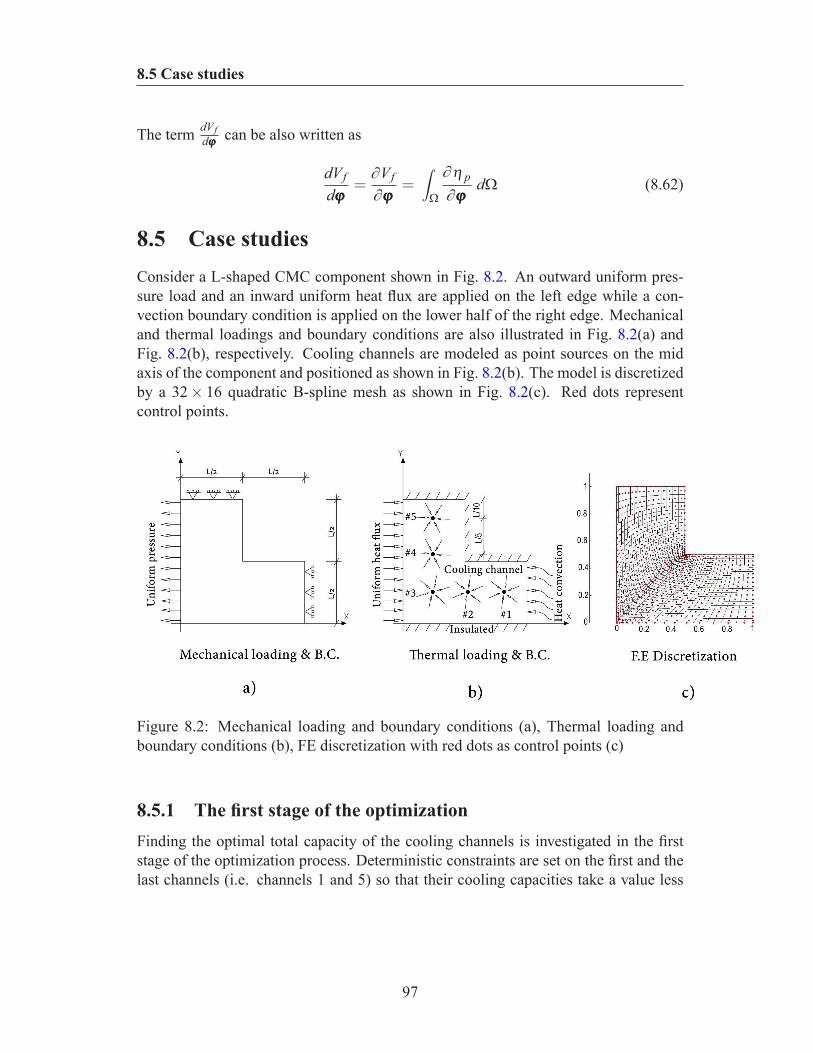
8.5 Case studies
The term dV fdϕϕϕ can be also written as
dV fdϕϕϕ
=∂V f∂ϕϕϕ
=∫
Ω
∂η p∂ϕϕϕ
dΩ (8.62)
8.5 Case studiesConsider a L-shaped CMC component shown in Fig. 8.2. An outward uniform pres-sure load and an inward uniform heat flux are applied on the left edge while a con-vection boundary condition is applied on the lower half of the right edge. Mechanicaland thermal loadings and boundary conditions are also illustrated in Fig. 8.2(a) andFig. 8.2(b), respectively. Cooling channels are modeled as point sources on the midaxis of the component and positioned as shown in Fig. 8.2(b). The model is discretizedby a 32× 16 quadratic B-spline mesh as shown in Fig. 8.2(c). Red dots representcontrol points.
Figure 8.2: Mechanical loading and boundary conditions (a), Thermal loading andboundary conditions (b), FE discretization with red dots as control points (c)
8.5.1 The first stage of the optimizationFinding the optimal total capacity of the cooling channels is investigated in the firststage of the optimization process. Deterministic constraints are set on the first and thelast channels (i.e. channels 1 and 5) so that their cooling capacities take a value less
97
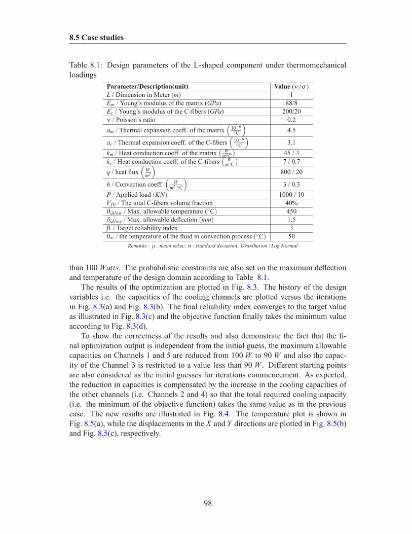
8.5 Case studies
Table 8.1: Design parameters of the L-shaped component under thermomechanicalloadings
Parameter/Description(unit) Value (ν/σ)L / Dimension in Meter (m) 1Em / Young’s modulus of the matrix (GPa) 88/8Ec / Young’s modulus of the C-fibers (GPa) 200/20ν / Poisson’s ratio 0.2am / Thermal expansion coeff. of the matrix
(10−6C
)4.5
ac / Thermal expansion coeff. of the C-fibers(
10−6C
)3.1
km / Heat conduction coeff. of the matrix( W
mC)
45 / 3kc / Heat conduction coeff. of the C-fibers
( WmC)
7 / 0.7q / heat flux
(Wm2
)800 / 20
h / Convection coeff.(
Wm2.C
)3 / 0.3
P / Applied load (KN) 1000 / 10Vf 0 / The total C-fibers volume fraction 40%θallow / Max. allowable temperature (C) 450δallow / Max. allowable deflection (mm) 1.5β / Target reliability index 3θ∞ / the temperature of the fluid in convection process (C) 50
Remarks : µ : mean value, σ : standard deviation, Distribution : Log Normal
than 100 Watts. The probabilistic constraints are also set on the maximum deflectionand temperature of the design domain according to Table 8.1.
The results of the optimization are plotted in Fig. 8.3. The history of the designvariables i.e. the capacities of the cooling channels are plotted versus the iterationsin Fig. 8.3(a) and Fig. 8.3(b). The final reliability index converges to the target valueas illustrated in Fig. 8.3(c) and the objective function finally takes the minimum valueaccording to Fig. 8.3(d).
To show the correctness of the results and also demonstrate the fact that the fi-nal optimization output is independent from the initial guess, the maximum allowablecapacities on Channels 1 and 5 are reduced from 100 W to 90 W and also the capac-ity of the Channel 3 is restricted to a value less than 90 W . Different starting pointsare also considered as the initial guesses for iterations commencement. As expected,the reduction in capacities is compensated by the increase in the cooling capacities ofthe other channels (i.e. Channels 2 and 4) so that the total required cooling capacity(i.e. the minimum of the objective function) takes the same value as in the previouscase. The new results are illustrated in Fig. 8.4. The temperature plot is shown inFig. 8.5(a), while the displacements in the X and Y directions are plotted in Fig. 8.5(b)and Fig. 8.5(c), respectively.
98

8.5 Case studies
Figure 8.3: Optimization results for target reliability index equal to 3 and with follow-ing constraints on channels #1 and #5: Q1 ≤ 100 and Q5 ≤ 100; Obtained optimumdesign variables: Q1 = 80.71, Q2 = 105.50, Q3 = 106.27, Q4 = 107.02, Q5 = 83.82;Optimized cost = 483.32 W
99
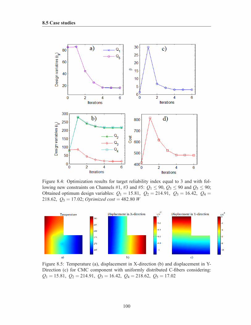
8.5 Case studies
Figure 8.4: Optimization results for target reliability index equal to 3 and with fol-lowing new constraints on Channels #1, #3 and #5: Q1 ≤ 90, Q3 ≤ 90 and Q5 ≤ 90;Obtained optimum design variables: Q1 = 15.81, Q2 = 214.91, Q3 = 16.42, Q4 =218.62, Q5 = 17.02; Optimized cost = 482.80 W
Figure 8.5: Temperature (a), displacement in X-direction (b) and displacement in Y-Direction (c) for CMC component with uniformly distributed C-fibers considering:Q1 = 15.81, Q2 = 214.91, Q3 = 16.42, Q4 = 218.62, Q5 = 17.02
100
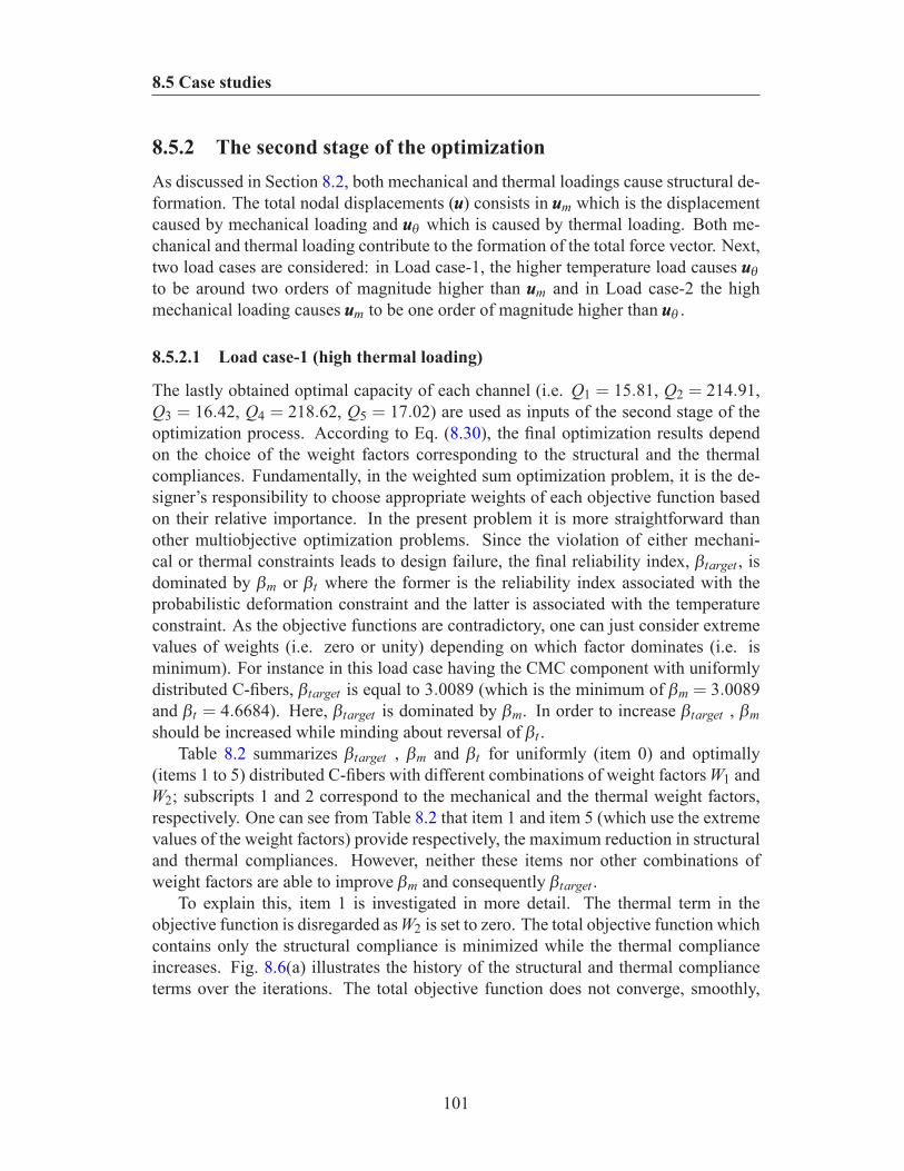
8.5 Case studies
8.5.2 The second stage of the optimizationAs discussed in Section 8.2, both mechanical and thermal loadings cause structural de-formation. The total nodal displacements (uuu) consists in uuum which is the displacementcaused by mechanical loading and uuuθ which is caused by thermal loading. Both me-chanical and thermal loading contribute to the formation of the total force vector. Next,two load cases are considered: in Load case-1, the higher temperature load causes uuuθto be around two orders of magnitude higher than uuum and in Load case-2 the highmechanical loading causes uuum to be one order of magnitude higher than uuuθ .
8.5.2.1 Load case-1 (high thermal loading)
The lastly obtained optimal capacity of each channel (i.e. Q1 = 15.81, Q2 = 214.91,Q3 = 16.42, Q4 = 218.62, Q5 = 17.02) are used as inputs of the second stage of theoptimization process. According to Eq. (8.30), the final optimization results dependon the choice of the weight factors corresponding to the structural and the thermalcompliances. Fundamentally, in the weighted sum optimization problem, it is the de-signer’s responsibility to choose appropriate weights of each objective function basedon their relative importance. In the present problem it is more straightforward thanother multiobjective optimization problems. Since the violation of either mechani-cal or thermal constraints leads to design failure, the final reliability index, βtarget , isdominated by βm or βt where the former is the reliability index associated with theprobabilistic deformation constraint and the latter is associated with the temperatureconstraint. As the objective functions are contradictory, one can just consider extremevalues of weights (i.e. zero or unity) depending on which factor dominates (i.e. isminimum). For instance in this load case having the CMC component with uniformlydistributed C-fibers, βtarget is equal to 3.0089 (which is the minimum of βm = 3.0089and βt = 4.6684). Here, βtarget is dominated by βm. In order to increase βtarget , βmshould be increased while minding about reversal of βt .
Table 8.2 summarizes βtarget , βm and βt for uniformly (item 0) and optimally(items 1 to 5) distributed C-fibers with different combinations of weight factors W1 andW2; subscripts 1 and 2 correspond to the mechanical and the thermal weight factors,respectively. One can see from Table 8.2 that item 1 and item 5 (which use the extremevalues of the weight factors) provide respectively, the maximum reduction in structuraland thermal compliances. However, neither these items nor other combinations ofweight factors are able to improve βm and consequently βtarget .
To explain this, item 1 is investigated in more detail. The thermal term in theobjective function is disregarded as W2 is set to zero. The total objective function whichcontains only the structural compliance is minimized while the thermal complianceincreases. Fig. 8.6(a) illustrates the history of the structural and thermal complianceterms over the iterations. The total objective function does not converge, smoothly,
101

8.5 Case studies
Table 8.2: Summary of optimization results in Load case-1 for uniformly and optimallydistributed C-fibers with different combinations of weight factors
Total Structural ThermalItem W1/W2 objective compliance βm compliance βt βtarget
Uniform 0 - 1 1 3.0089 1 4.6684 3.00891 1/0 0.959 0.959 2.4976 1.083 4.6835 2.4976
Optimally 2 0.75/0.25 0.961 0.972 2.3783 0.929 4.6753 2.3783distributed 3 0.5/0.5 0.950 0.979 2.3518 0.920 4.6700 2.3518
C-fibers 4 0.25/0.75 0.935 0.982 2.3748 0.920 4.6689 2.37485 0/1 0.920 0.9840 2.4 0.920 4.6686 2.4
towards the minimum value.This undesired phenomenon that a decrease in the structural compliance yields to
a larger maximum structural deformation (which consequently causes lower βm) iscaused by the coupling between the thermal and the mechanical fields and the con-tradictory effects of C-fibers on these fields. In a typical elastic problem, when thestiffness increases as the force vector remains unchanged, the maximum structural de-formation will decrease. In the coupled thermoelastic problem, the forces inducedby the temperature field and consequently the total force vector does not remain un-changed. According to Eq. (8.12), the force induced by the temperature field willchange when the Young’s modulus, thermal expansion coefficient or nodal tempera-tures deviate. Since all of these items are functions of the volume fraction of C-fibers,the final magnitude of the force vector depends on the distribution of the C-fibers.Thus, any increase or decrease in the maximum deflection of a CMC component de-pends on the changes of structural stiffness and force induced by the temperature fieldand should be evaluated case by case based on the constituent material properties andthe loading conditions.
To gain better insight into this issue, the same problem is solved assuming the me-chanical and thermal fields are decoupled. This is accomplished by setting the thermalexpansion coefficients of both the C-fibers and the matrix to zero. Fig. 8.6(b) showsthe results for the decoupled problem. In this case the objective function smoothlyconverges towards the minimum value and the optimization process is stable.
In item 5 (W1 = 0 and W2 = 1) the structural term in the objective function isdisregarded. Thus the total objective function consists only by the thermal compliancecontribution. The optimal distribution of the C-fibers and the history of the objectivefunctions over the iterations are presented in Fig. 8.7. As the mechanical field doesn’taffect the thermal field, the optimization process is stable and the objective functionsmoothly converge towards its minimum value, though the problem is coupled.
102
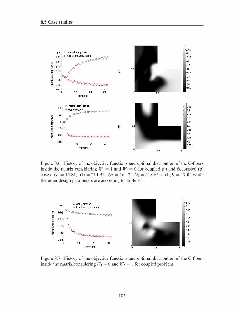
8.5 Case studies
Figure 8.6: History of the objective functions and optimal distribution of the C-fibersinside the matrix considering W1 = 1 and W2 = 0 for coupled (a) and decoupled (b)cases. Q1 = 15.81, Q2 = 214.91, Q3 = 16.42, Q4 = 218.62 and Q5 = 17.02 whilethe other design parameters are according to Table 8.1
Figure 8.7: History of the objective functions and optimal distribution of the C-fibersinside the matrix considering W1 = 0 and W2 = 1 for coupled problem
103

8.5 Case studies
8.5.2.2 Load case-2 (high mechanical loading)
Now, the applied mechanical load is increased so that it dominates the thermal one.Table 8.3 includes the new design parameters. Other design parameters remain un-changed according to Table 8.1. The results of the optimization for this load case are
Table 8.3: New design parameters of the L-shaped component under thermomechani-cal loading
Parameter / Description (unit) Value (µ/σ)P / Applied load (KN) 1000000 / 10000σallow / Max. allowable deflection (mm) 50
other design parameters according to Table 8.1
summarized in Table 8.4. Item 0 refers to uniformly distributed C-fibers. In item 1the thermal term is disregarded and the total objective function just includes the struc-tural term while item 2 acts reversely. Fig. 8.8(a) shows the optimal distribution of
Table 8.4: Summary of optimization results in Load case-2 for uniformly and optimallydistributed C-fibers with different combinations of weight factors
Structural ThermalItem Wm/Wt compliance βm compliance βt βtarget
Uniform 0 - 1 2.8916 1 4.6684 2.8913Optimal 1 1 / 0 0.8963 4.4259 1.0814 4.5803 4.34
2 0 / 1 1.060 2.3323 0.920 4.6686 2.3322
C-fibers and the history of the objective functions for item 1, respectively. Decreas-ing the structural compliance yields an increase in the structural stiffness. Since theC-fibers distribution is changed, fff also changes. Contrary to the previous case, as thethermal force is smaller than the mechanical force, its deviation does not influence thetotal force vector severely, resulting in a decrease in the maximum structural deflectionand consequently a considerable increase in βm and eventually βtarget .
The optimal distribution of C-fibers and the history of objective functions for dif-ferent weights are illustrated in Fig. 8.8(b). The structural compliance is disregardedin the total objective function and increases while the objective function (i.e. ther-mal compliance) is minimized. Although the thermal compliance is decreased, thereduction in maximum temperature and consequently in βt is trifle and not sensible.However, as βm decreases (due to the increase in structural compliance), βtarget alsodecreases.
104
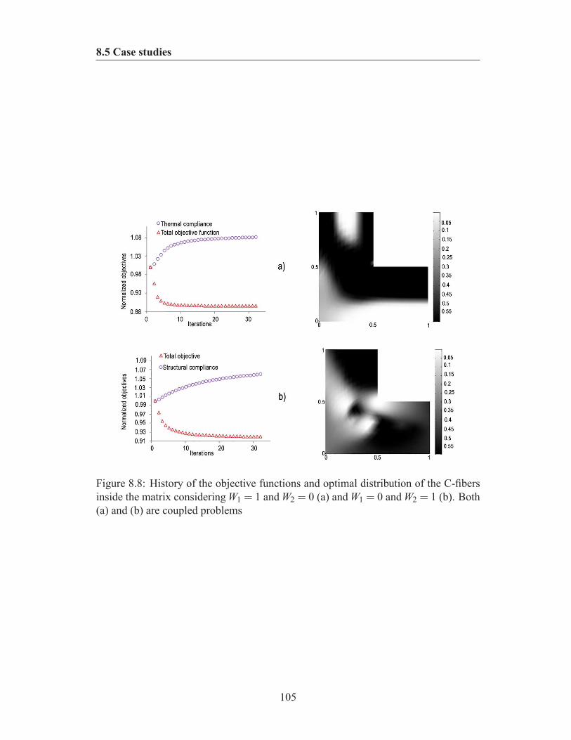
8.5 Case studies
Figure 8.8: History of the objective functions and optimal distribution of the C-fibersinside the matrix considering W1 = 1 and W2 = 0 (a) and W1 = 0 and W2 = 1 (b). Both(a) and (b) are coupled problems
105
8.6 Concluding remarks
8.6 Concluding remarksCeramic matrix composites which are manufactured by adding reinforcements suchas carbon fibers to a ceramic matrix show improved toughness properties in compar-ison with pure ceramics. Usually, components made of CMCs are cooled by internalcooling channels because typical C-fibers are vulnerable to high temperature oxidiz-ing atmospheres. Firstly, the presented computational platform efficiently optimizesthe capacity of cooling channels using RBDO approach. A series system reliabilityconcept is adopted as a union of mechanical and thermal failure subsets. Secondly,the optimizer is supposed to increase the reliability of the component by optimallydistributing the C-fibers inside the matrix within the design domain. Numerical re-sults for the performed case studies demonstrate that optimal distribution of C-fiberscan decrease structural and thermal compliances. In the decoupled elastic and ther-mal problems, the former yields an increase in βm(the reliability index associated withthe probabilistic deformation constraint) and the latter in an increase in βt(the relia-bility index associated with the probabilistic thermal constraint). But, in the coupledthermoelastic problem, any prediction about final reliability indices depends on fiberand matrix constitutive material properties and contribution of mechanical and ther-mal loadings on the global force vector. When the mechanical loading dominates thethermal loading, fiber distribution can show promising advantage to have more reliabledesign by increasing βm and consequently βtarget(the final reliability index). However,its role for increasing the reliability index corresponding to thermal constraint is neg-ligible.
106
Chapter 9
Application 3: A level-set based IGAformulation for topology optimizationof flexoelectric materials
9.1 IntroductionThe piezoelectric effect, which only exists in materials with non-centrosymmetric crys-tal structures, refers to a linear dependence between the electric polarization, PPP and themechanical strain, εεε given by
Pi = pi jkε jk (9.1)
where ppp is the third order piezoelectric tensor [Sharma et al., 2007 ; Nanthakumaret al., 2016 ; Nanthakumar et al., 2014 and Nanthakumar et al., 2013]. In contrast topiezoelectricity, flexoelectricity is possible in all dielectrics, including those with cen-trosymmetric crystal structures, and is thus a more general electromechanical couplingmechanism. When flexoelectric effects are accounted for, the polarization is written as
Pi = pi jkε jk +µi jkl∂ε jk∂xl
(9.2)
where the electric polarization exhibits a linear response to the gradient of mechanicalstrain [Yudin & Tagantsev, 2013]. In Eq. (9.2) µi jkl are the flexoelectric coefficients;the first term on the right hand side is zero for non-piezoelectric materials.
Flexoelectricity in solids was introduced by Mashkevich & Tolpygo, 1957 but re-ceived little attention, likely because the flexoelectric effect is relatively insignificantfor bulk crystalline materials. However recent developments in nanotechnology haveshed a new light on flexoelectricity as a size dependent phenomenon due to the largestrain gradients that are obtainable at small length scales, or alternatively in soft mate-rials like biological membranes [Ahmadpour & Sharma, 2015]. For additional recent
107
9.1 Introduction
reviews on flexoelectricity interested readers are referred to [Nguyen et al., 2013] and[Zubko et al., 2013].
While the theoretical basis for flexoelectricity in dielectrics has been developedin detail [Sharma et al., 2007 ; Majdoub et al., 2009 and Sharma et al., 2010], therehave been a correspondingly small number of numerical studies. Recently, Abdollahiet al., 2014 presented a computational framework to evaluate the flexoelectric effectin dielectric solids using a meshfree method in 2D [Abdollahi et al., 2014] and 3D[Abdollahi et al., 2015]. They showed that available simplified analytical solutionsonly provide order of magnitude estimates in comparison with a more general modelwhich considers the multidimensional coupling effects.
Topology optimization is a powerful approach that optimizes the material distribu-tion within the design domain. The first computational model for topology optimiza-tion was presented by Bendse & Kikuchi, 1988. Topology optimization has since beensuccessfully applied to a variety of applications such as structural design [Sigmund,2001a], compliant mechanism [Sigmund, 1997] and microelectromechanical system[Sigmund, 2001b and Nanthakumar et al., 2015]. To the author’s best of knowledge,employing topology optimization for dielectric solids in order to enhance their flexo-electric behavior has not been done to-date.
Various techniques have been developed for topology optimization. Among them,the Solid Isotropic Material with Penalization (SIMP) technique [Rozvany et al., 1992]is very common due to its simplicity. Although this technique has been widely appliedto different problems, researchers have encountered difficulties with its numerical sta-bility in some multiphysics and multiconstraint problems [Wang et al., 2003]. Fur-thermore, in multiphysics problems the different sets of penalization parameters willdirectly and noticeably impact the final results in terms of the stability of the solutionand the distinct void-solid representation.
To overcome the above mentioned difficulties, the Level Set Method (LSM) [Osher& Sethian, 1988] for topology optimization is employed here in order to exploit itsintrinsic flexibility in handling topological changes. In the LSM, the boundaries ofthe domain are implicitly represented with a scalar level set function which changesin time, providing unique benefits such as smooth boundaries and distinct interfaces,integrated shape and topology optimization. IGA is also used instead of standard FEMbecause the fourth order PDEs of flexoelectricity demand at least C1 continuous basisfunctions in a Galerkin method [Abdollahi et al., 2014]. IGA also enables using thesame data set for the analysis and the optimization as well as an exact representationof the geometry (see Chapter 2 ).
108
9.2 Flexoelectricity: theory and formulation
9.2 Flexoelectricity: theory and formulationFor a linear dielectric solid possessing only the piezoelectric effect, the electric en-thalpy density, H , is a function of εεε and EEE, i.e. H (εi j,Ei). When flexoelectric effectsare accounted for, the enthalpy density H also becomes a function of the strain gradi-ent and electric field gradient. Thus
H (εi j,Ei,ε jk,l,Ei, j) =12
Ci jklεi jεkl − eiklEiεkl +(di jklEi, jεkl + fi jklEiε jk,l)−12κi jEiE j
(9.3)where Ei = −θ,i is the electric field; θθθ is the electric potential; εεε is the mechanicalstrain; eee is the third-order tensor of piezoelectricity; κκκ is the second-order dielectrictensor; CCC is the fourth-order elasticity tensor; fff is the fourth-order direct flexoelectrictensor and ddd is the fourth-order converse flexoelectric tensor [Abdollahi et al., 2014].Let’s consider the terms in the brackets on the RHS of Eq. (9.3) containing the directand reverse flexoelectric effects. Integrating these terms over the volume and usingintegration by parts and the Gauss divergence theorem on the first term yields
∫
Ω(di jklEi, jεkl + fi jklEiε jk,l)dΩ=
∫
Ωdi jklEi, jεkldΩ+
∫
Ωfi jklEiε jk,ldΩ
=∫
∂Ωdi jklEiεklds−
∫
Ωdi jklEiεkl, jdΩ+
∫
Ωfi jklEiε jk,ldΩ
=∫
Ω( fi jklEiε jk,l −di jklEiεkl, j)dΩ+
∫
∂Ωdi jklEiεklds
=−∫
Ω(dil jk − fi jkl)Eiε jk,ldΩ+
∫
∂Ωdi jklEiεklds
=−∫
Ωµi jklEiε jk,ldΩ+
∫
∂Ωdi jklEiεklds
(9.4)
which is expressed in terms of only one material tensor, µµµ where µi jkl = dil jk − fi jkl .Therefore, one can rewrite Eq. (9.3) as
H (εi j,Ei,ε jk,l) =12
Ci jklεi jεkl − eiklEiεkl −µi jklEiε jk,l −12κi jEiE j (9.5)
For a pure piezoelectric material we have
σi j =∂H
∂εi jand Di =−
∂H
∂Ei(9.6)
while in the presence of flexoelectricity, the electromechanical stresses including theusual (σi j/Di), higher-order (σi jk/Di j) and physical (σi j/Di) ones are defined throughthe following relations:
σi j =∂H
∂εi jand Di =−
∂H
∂Ei(9.7)
109
9.2 Flexoelectricity: theory and formulation
σi jk =∂H
∂εi j,kand Di j =−
∂H
∂Ei, j(9.8)
σi j = σi j − σi jk,k and Di = Di − Di j, j (9.9)
thusσi j = σi j − σi jk,k =Ci jklεkl − eki jEk +µli jkEl,k (9.10)
Di = Di − Di j, j = eiklεkl +κi jE j +µi jklε jk,l (9.11)
Since Di j has no contribution in Eq. (9.5) thus, the essential and natural electricalboundary conditions are the same as electrostatics. So,
θ = θ on Γθ (9.12)
Dini =−ω on ΓD (9.13)
Γθ ∪ΓD = ∂Ω and Γθ ∩ΓD = /0 (9.14)
where θ and ω are the prescribed electric potential and surface change density; ni isthe unit normal to the boundary ∂Ω of the domain Ω.
For the mechanical boundary conditions we have
ui = ui on Γu (9.15)
tk = n j(σ jk − σi jk,l)−D j(niσi jk)− (Dpnp)nin jσi jk = tk on Γt (9.16)
Γu ∪Γt = ∂Ω and Γu ∩Γt = /0 (9.17)
where ui and tk are the prescribed mechanical displacements and tractions; D j is thesurface gradient operator. In addition to these, the strain gradients result in other typesof boundary conditions as follows
ui, jn j = vi on Γv (9.18)
nin jσi jk = rk on Γr (9.19)
Γv ∪Γr = ∂Ω and Γv ∩Γr = /0 (9.20)
110
9.2 Flexoelectricity: theory and formulation
where υ i and rk are the prescribed normal derivative of displacement and the higherorder traction, respectively. Eq. (9.7) and Eq. (9.8) can be rewritten as
∂H = σi j∂εi j (9.21)
∂H = σi jk∂εi j,k (9.22)
∂H =−Di∂Ei (9.23)
and then by integrating over Ω we obtain
H =12
∫
Ω(σi jεi j + σi jkεi j,k − DiEi)dΩ (9.24)
where H is the total electrical enthalpy.The work done by the external surface mechanical and electrical forces can be
written asWext =
∫
Γtt iuidS−
∫
ΓDωθdS (9.25)
The kinetic energy for the system is also defined as
KE =12
∫
Ωρ uiuidΩ (9.26)
where ρ denotes the density and the superimposed dot indicate time derivative. UsingHamilton principle without the damping term we have
δ∫ t2
t1(KE −H +Wext)dt = 0 (9.27)
and
δ∫ t2
t1
(12
∫
Ωρ uiuidΩ−
12
∫
Ω(σi jεi j + σi jkεi j,k − DiEi)dΩ
+∫
Γtt iuidS−
∫
ΓDωθdS
)dt = 0
(9.28)
moving the variation operation into the integral operations we obtain
∫ t2
t1
(12
∫
Ωδ (ρ uiui)dΩ−
12
∫
Ωδ (σi jεi j + σi jkεi j,k − DiEi)dΩ
+∫
Γtt iδuidS−
∫
ΓDωδθdS
)dt = 0
(9.29)
111
9.3 Discretization
by changing the order of operations and using the chain rule of variation we have∫ t2
t1
[12
∫
Ωδ (ρ uiui)dΩ
]dt =−
∫ t2
t1
[∫
Ωρ(δuiui)dΩ
]dt (9.30)
∫ t2
t1
[12
∫
Ωδ (σi jεi j + σi jkεi j,k − DiEi)dΩ
]dt =
∫ t2
t1
[∫
Ω(σi jδεi j + σi jkδεi j,k − DiδEi)dΩ
]dt
(9.31)
Eq. (9.29) now becomes
∫ t2
t1
(−∫
Ωρ(δuiui)dΩ−
∫
Ω(σi jδεi j + σi jkδεi j,k − DiδEi)dΩ
+∫
Γtt iδuidS−
∫
ΓDωδθdS
)dt = 0
(9.32)
To satisfy Eq. (9.32) for all possible choices of uuu, the integrand of the time integrationhas to vanish, which leads to∫
Ωρ(δuiui)dΩ+
∫
Ω(σi jδεi j + σi jkδεi j,k − DiδEi)dΩ−
∫
Γtt iδuidS+
∫
ΓDωδθdS = 0
(9.33)The inertia term is neglected for a static problem yielding
∫
Ω(σi jδεi j + σi jkδεi j,k − DiδEi)dΩ−
∫
Γtt iδuidS+
∫
ΓDωδθdS = 0 (9.34)
Substituting Eqs. (9.7)- (9.11) into Eq. (9.34)) yields∫
Ω
(Ci jklδεi jεkl − eki jEkδεi j −µli jkElδεi j,k −κi jδEiE j − eiklδEiεkl −µi jklδEiε jk,l
)dΩ
−∫
Γtt iδuidS+
∫
ΓDωδθdS = 0
(9.35)
9.3 DiscretizationIn this section the NURBS basis functions are employed to approximate displacementuuu and electric potential θθθ fields as well as their derivatives according to
uh(x,y) =n
∑i=1
m
∑j=1
N p,qi, j (ξ ,η)u
ei j = (NNNu)
Tuuue (9.36)
112
9.3 Discretization
θh(x,y) =n
∑i=1
m
∑j=1
N p,qi, j (ξ ,η)θ
ei j = (NNNθ )
Tθθθ e (9.37)
∂ juh = ∂ jNNNuuuue = (BBBu)Tuuue = εεε (9.38)
∂ jθh = ∂ jNNNθθθθ e = (BBBθ )Tθθθ e =−EEE (9.39)
∂ j∂kuh = ∂ j∂kNNNuuuue = (HHHu)Tuuue (9.40)
where the superscript e denotes nodal parameters at the control points; BBBu, BBBθ andHHHu are the matrices containing the gradient and Hessian of the corresponding basisfunctions (i.e. NNNu and NNNθ ) which are defined as
BBBu =
∂N1∂x 0 ∂N1
∂y∂N2∂x 0 ∂N2
∂y...
......
∂Nn∂x 0 ∂Nn
∂y0 ∂N1
∂y∂N1∂x
0 ∂N2∂y
∂N2∂x
......
...0 ∂Nn
∂y∂Nn∂x
(9.41)
BBBθ =
∂N1∂x
∂N1∂y
......
∂Nn∂x
∂Nn∂y
(9.42)
HHHu =
∂ 2N1∂x2 0 ∂ 2N1
∂y∂x∂ 2N1∂x∂y 0 ∂ 2N1
∂y2
∂ 2N2∂x2 0 ∂ 2N2
∂y∂x∂ 2N2∂x∂y 0 ∂ 2N2
∂y2
......
......
......
∂ 2Nn∂x2 0 ∂ 2Nn
∂y∂x∂ 2Nn∂x∂y 0 ∂ 2Nn
∂y2
0 ∂ 2N1∂y∂x
∂ 2N1∂x2 0 ∂ 2N1
∂y2∂ 2N1∂x∂y
0 ∂ 2N2∂y∂x
∂ 2N2∂x2 0 ∂ 2N2
∂y2∂ 2N2∂x∂y
......
......
......
0 ∂ 2Nn∂y∂x
∂ 2Nn∂x2 0 ∂ 2Nn
∂y2∂ 2Nn∂x∂y
(9.43)
113
9.3 Discretization
By substituting Eq. (9.36) to Eq. (9.40) into Eq. (9.35) we obtain after some algebrathe following discrete system of equations
[AAAUU AAAUθAAAθU AAAθθ
] [UUUθθθ
]=
[fffUfff θ
](9.44)
whereAAAUU =∑
e
∫
Ωe(BBBu)CCC(BBBu)
T dΩe (9.45)
AAAUθ =∑e
∫
Ωe
[(BBBu)eee(BBBθ )T +(HHHu)µµµT (BBBθ )T ]dΩe (9.46)
AAAθU =∑e
∫
Ωe
[(BBBθ )eeeT (BBBu)
T +(BBBθ )µµµ(HHHu)T ]dΩe (9.47)
AAAθθ =−∑e
∫
Ωe(BBBθ )κκκ(BBBθ )T dΩe (9.48)
fffU =∑e
∫
Γte
NNNTu tttΓdΓte (9.49)
fff θ =−∑e
∫
ΓDe
NNNTθωdΓDe (9.50)
In Eqs. (9.45) - (9.50), the subscript, e, inΩe, Γte and ΓDe denotes the eth finite elementwhere Ω= ∪eΩe. Moreover, CCC,κκκ,eee and µµµ can be written in matrix form as
CCC =
(E
(1+ν)(1−2ν)
)
1−ν ν 0ν 1−ν 00 0
(12 −ν
)
(9.51)
κκκ =
[κ11 00 κ33
](9.52)
eeeT =
[0 0 e15
e31 e33 0
](9.53)
µµµ =
[µ11 µ12 0 0 0 µ440 0 µ44 µ12 µ11 0
](9.54)
Interested readers can also refer to [Sharma et al., 2007] and [Majdoub et al., 2009]for more details about the theory of flexoelectricity.
114
9.4 Level Set Method (LSM) and optimization problem
9.4 Level Set Method (LSM) and optimization problem
9.4.1 LSMIn this section the LSM fundamentals are briefly described. Let’s assume Ω⊂ D ⊂R
d
(d = 2 or 3), where D is the whole structural domain including all admissible shapes,Ω. A level set function Φ(xxx) is defined as
Solid : Φ(xxx)> 0 ∀xxx ∈Ω\∂ΩBoundary : Φ(xxx) = 0 ∀xxx ∈ ∂Ω∩DVoid : Φ(xxx)< 0 ∀xxx ∈ D\Ω
(9.55)
The design boundary Γ(xxx) is then implicitly represented by the iso-surface (in this textzero surface) of Φ(xxx) such that
Γ(xxx) =
xxx ∈ Rd|Φ(xxx) = 0
(9.56)
and by letting the level set function dynamically change in time, the dynamic model isexpressed as
Γ(t) =
xxx(t) ∈ Rd|Φ(xxx(t), t) = 0
(9.57)
and by differentiating both sides of Eq. (9.57) with respect to time and applying thechain rule we have
∂Φ(xxx(t), t)∂ t
+∇Φ(xxx(t), t) ·dxdt
= 0 (9.58)
where VVV = dxdt is the velocity vector of the design boundary and its normal component
is Vn =VVV ·nnn where nnn = ∇Φ|∇Φ| is the unit outward normal to the boundary. Eq. (9.58) is
the so-called Hamilton-Jacobi equation and can be written in the form of
∂Φ∂ t
+Vn|∇Φ|= 0 (9.59)
which defines an initial value problem for the time dependent function Φ. In opti-mization process Vn is the movement of a point on a surface driven by the objective ofthe optimization. The optimal structural boundary is then expressed as a solution ofEq. (9.59) obtained by a so called ”up-wind scheme” [Wang et al., 2003].
In this section, the LS function at the point (x,y) is denoted by Φ(x,y) and definedas
Φ(x,y) =n
∑i=1
m
∑j=1
N p,qi, j (ξ ,η)ϕi, j (9.60)
where N p,qi, j and ϕi, j are B-spline basis functions and corresponding nodal values of LS,
respectively. ϕi, j are the only design variables which are defined on the control pointsmesh being set as the signed distance to the given boundary of the initial design.
115
9.4 Level Set Method (LSM) and optimization problem
The density-based approach is used for mapping the geometry to the mechanicalmodel. Using this approach, the material domain (density field 0 < ρmin ≤ ρ(xxx) ≤ 1)flows through a fixed discretization of the design domain in each optimization iteration.In other words, these densities are used to directly scale the stiffness of the material,known as the ”Ersatz material” approach. ρ = 1 represents the solid material whileρmin = 1e−4 is the lower bound to avoid singularity of the stiffness matrix.
Using point-wise mapping to control an element-wise constant density distributionwe have
ρe = (1−ρmin)H(Φ(Xe))+ρmin (9.61)
where Xe is the center of a finite element e. H(Φ) is a smooth approximation of theHeaviside function defined by [ Wang et al., 2003]
H(Φ) =
0 f or Φ<−h
−14(Φ
h)3
+ 34(Φ
h)+ 1
2 f or −h ≤Φ≤ h
1 f or h <Φ
(9.62)
Having ρ , the volume integrals of some functional f over a material domain can thenbe defined as ∫
Ωf dV =
∫
Df H(Φ)dV ≈
∫
Dfρ(Φ)dV (9.63)
Meanwhile ρ is embedded in the electromechanical problem as
M(x,y) = ρ(Φ)M0 with MMM0 =CCC,eee,κκκ,µµµ (9.64)
where CCC,eee,κκκ and µµµ denote elastic, piezoelectricity, permittivity and flexoelectricitytensors, respectively. Subscript 0 represents properties of the solid material.
The derivative of the density function with respect to the level set nodal values isobtained by
∂ρe∂ϕi, j
= (1−ρmin)δ (Φ(Xe))∂Φ(Xe)
∂ϕi, j(9.65)
where δ (Φ) = ∂ H∂Φ is the approximate Dirac delta function defined by
δ (Φ) =
3(1−ρmin)4h
(1−(Φ
h)2)
f or−h ≤Φ≤ h
0 otherwise(9.66)
and ∂Φ(Xe)∂ϕi, j
is calculated by∂Φ(Xe)
∂ϕi, j= Rp,q
i, j (ξ ,η) (9.67)
116
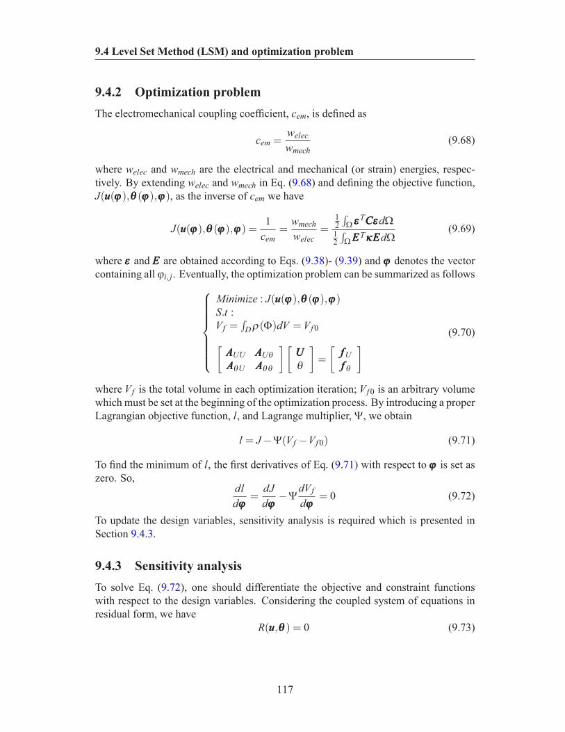
9.4 Level Set Method (LSM) and optimization problem
9.4.2 Optimization problemThe electromechanical coupling coefficient, cem, is defined as
cem =welecwmech
(9.68)
where welec and wmech are the electrical and mechanical (or strain) energies, respec-tively. By extending welec and wmech in Eq. (9.68) and defining the objective function,J(uuu(ϕϕϕ),θθθ(ϕϕϕ),ϕϕϕ), as the inverse of cem we have
J(uuu(ϕϕϕ),θθθ(ϕϕϕ),ϕϕϕ) =1
cem=
wmechwelec
=12∫Ωεεε
TCCCεεεdΩ12∫ΩEEETκκκEEEdΩ
(9.69)
where εεε and EEE are obtained according to Eqs. (9.38)- (9.39) and ϕϕϕ denotes the vectorcontaining all ϕi, j. Eventually, the optimization problem can be summarized as follows
Minimize : J(uuu(ϕϕϕ),θθθ(ϕϕϕ),ϕϕϕ)S.t :V f =
∫Dρ(Φ)dV =V f 0
[AAAUU AAAUθAAAθU AAAθθ
][UUUθ
]=
[fffUfff θ
](9.70)
where V f is the total volume in each optimization iteration; V f 0 is an arbitrary volumewhich must be set at the beginning of the optimization process. By introducing a properLagrangian objective function, l, and Lagrange multiplier, Ψ, we obtain
l = J−Ψ(V f −V f 0) (9.71)
To find the minimum of l, the first derivatives of Eq. (9.71) with respect to ϕϕϕ is set aszero. So,
dldϕϕϕ
=dJdϕϕϕ
−ΨdV fdϕϕϕ
= 0 (9.72)
To update the design variables, sensitivity analysis is required which is presented inSection 9.4.3.
9.4.3 Sensitivity analysisTo solve Eq. (9.72), one should differentiate the objective and constraint functionswith respect to the design variables. Considering the coupled system of equations inresidual form, we have
R(uuu,θθθ) = 0 (9.73)
117
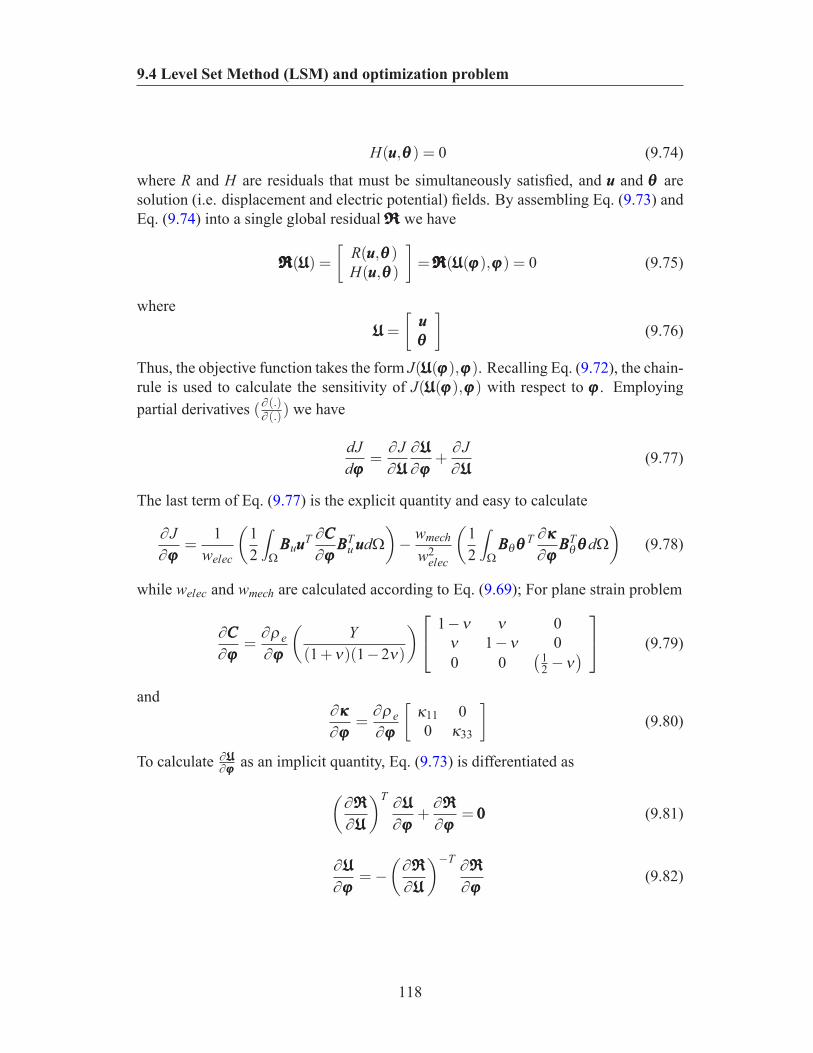
9.4 Level Set Method (LSM) and optimization problem
H(uuu,θθθ) = 0 (9.74)
where R and H are residuals that must be simultaneously satisfied, and uuu and θθθ aresolution (i.e. displacement and electric potential) fields. By assembling Eq. (9.73) andEq. (9.74) into a single global residual RRR we have
RRRRRRRRR(UUU) =
[R(uuu,θθθ)H(uuu,θθθ)
]=RRRRRRRRR(UUU(ϕϕϕ),ϕϕϕ) = 0 (9.75)
whereUUU=
[uuuθθθ
](9.76)
Thus, the objective function takes the form J(UUU(ϕϕϕ),ϕϕϕ). Recalling Eq. (9.72), the chain-rule is used to calculate the sensitivity of J(UUU(ϕϕϕ),ϕϕϕ) with respect to ϕϕϕ . Employingpartial derivatives (∂ (.)∂ (.)) we have
dJdϕϕϕ
=∂J∂UUU
∂UUU∂ϕϕϕ
+∂J∂UUU
(9.77)
The last term of Eq. (9.77) is the explicit quantity and easy to calculate
∂J∂ϕϕϕ
=1
welec
(12
∫
ΩBBBuuuuT ∂CCC
∂ϕϕϕBBBT
u uuudΩ)−
wmechw2
elec
(12
∫
ΩBBBθθθθT ∂κκκ
∂ϕϕϕBBBTθθθθdΩ
)(9.78)
while welec and wmech are calculated according to Eq. (9.69); For plane strain problem
∂CCC∂ϕϕϕ
=∂ρe∂ϕϕϕ
(Y
(1+ν)(1−2ν)
)
1−ν ν 0ν 1−ν 00 0
(12 −ν
)
(9.79)
and∂κκκ∂ϕϕϕ
=∂ρe∂ϕϕϕ
[κ11 00 κ33
](9.80)
To calculate ∂UUU∂ϕϕϕ as an implicit quantity, Eq. (9.73) is differentiated as
(∂RRR∂UUU
)T ∂UUU∂ϕϕϕ
+∂RRR∂ϕϕϕ
= 000 (9.81)
∂UUU∂ϕϕϕ
=−
(∂RRR∂UUU
)−T ∂RRR∂ϕϕϕ
(9.82)
118
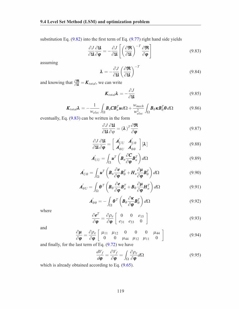
9.4 Level Set Method (LSM) and optimization problem
substitution Eq. (9.82) into the first term of Eq. (9.77) right hand side yields
∂J∂UUU
∂UUU∂ϕϕϕ
=−∂J∂UUU
[(∂RRR∂UUU
)−T ∂RRR∂ϕϕϕ
](9.83)
assuming
λλλ =−∂J∂UUU
(∂RRR∂UUU
)−T(9.84)
and knowing that ∂RRR∂UUU =KKKtotal , we can write
KKKtotalλλλ =−∂J∂UUU
(9.85)
KKKtotalλλλ =−1
welec
∫
ΩBBBuCCCBBBT
u uuudΩ+wmechw2
elec
∫
ΩBBBθκκκBBBT
θθθθdΩ (9.86)
eventually, Eq. (9.83) can be written in the form∂J∂UUU
∂UUU∂ϕ
= (λλλ )T ∂RRR∂ϕϕϕ
(9.87)
∂J∂UUU
∂UUU∂ϕϕϕ
=
[AAA′
UU AAA′
UθAAA′
θU AAA′
θθ
][λλλ ] (9.88)
AAA′
UU =∫
ΩuuuT(
BBBu∂CCC∂ϕϕϕ
BBBTu
)dΩ (9.89)
AAA′
Uθ =∫
ΩuuuT(
BBBu∂eee∂ϕϕϕ
BBBTθ +HHHu
∂µµµ∂ϕϕϕ
BBBTθ
)dΩ (9.90)
AAA′
θU =∫
ΩθθθT(
BBBθ∂eee∂ϕϕϕ
BBBTu +BBBθ
∂µµµ∂ϕϕϕ
HHHTu
)dΩ (9.91)
AAA′
θθ =−∫
ΩθθθT(
BBBθ∂κκκ∂ϕϕϕ
BBBTθ
)dΩ (9.92)
where∂eeeT
∂ϕϕϕ=∂ρe∂ϕϕϕ
[0 0 e15
e31 e33 0
](9.93)
and∂µµµ∂ϕϕϕ
=∂ρe∂ϕϕϕ
[µ11 µ12 0 0 0 µ440 0 µ44 µ12 µ11 0
](9.94)
and finally, for the last term of Eq. (9.72) we havedV fdϕϕϕ
=∂V f∂ϕϕϕ
=∫
Ω
∂ρe∂ϕϕϕ
dΩ (9.95)
which is already obtained according to Eq. (9.65).
119
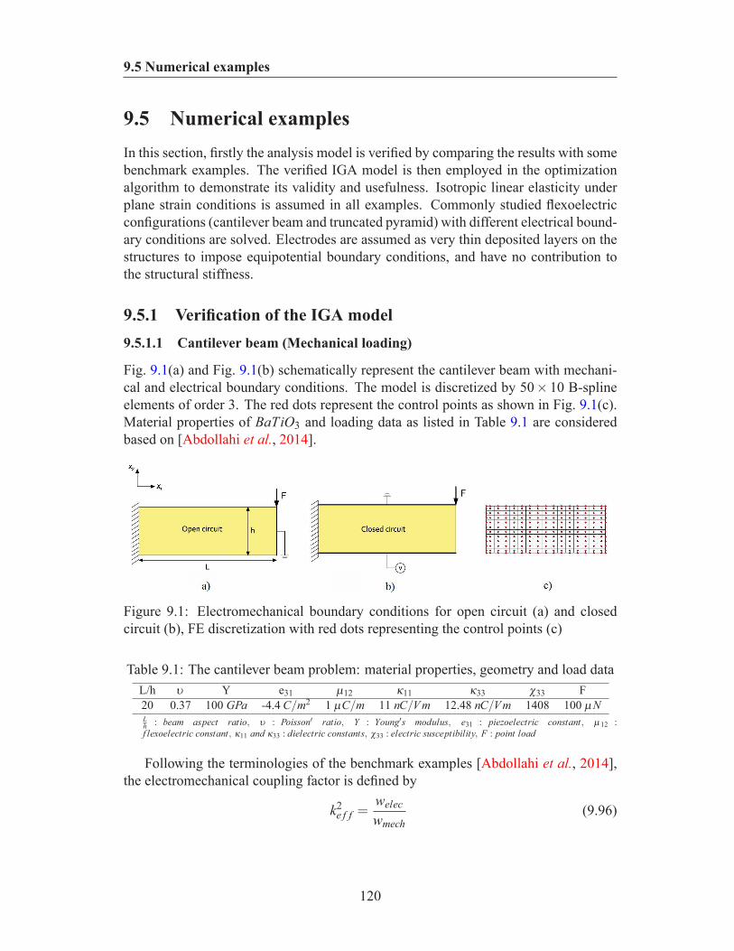
9.5 Numerical examples
9.5 Numerical examplesIn this section, firstly the analysis model is verified by comparing the results with somebenchmark examples. The verified IGA model is then employed in the optimizationalgorithm to demonstrate its validity and usefulness. Isotropic linear elasticity underplane strain conditions is assumed in all examples. Commonly studied flexoelectricconfigurations (cantilever beam and truncated pyramid) with different electrical bound-ary conditions are solved. Electrodes are assumed as very thin deposited layers on thestructures to impose equipotential boundary conditions, and have no contribution tothe structural stiffness.
9.5.1 Verification of the IGA model9.5.1.1 Cantilever beam (Mechanical loading)
Fig. 9.1(a) and Fig. 9.1(b) schematically represent the cantilever beam with mechani-cal and electrical boundary conditions. The model is discretized by 50× 10 B-splineelements of order 3. The red dots represent the control points as shown in Fig. 9.1(c).Material properties of BaTiO3 and loading data as listed in Table 9.1 are consideredbased on [Abdollahi et al., 2014].
Figure 9.1: Electromechanical boundary conditions for open circuit (a) and closedcircuit (b), FE discretization with red dots representing the control points (c)
Table 9.1: The cantilever beam problem: material properties, geometry and load dataL/h υ Y e31 µ12 κ11 κ33 χ33 F20 0.37 100 GPa -4.4 C/m2 1 µC/m 11 nC/V m 12.48 nC/V m 1408 100 µNLh : beam aspect ratio, υ : Poisson′ ratio, Y : Young′s modulus, e31 : piezoelectric constant, µ12 :f lexoelectric constant, κ11 and κ33 : dielectric constants, χ33 : electric susceptibility, F : point load
Following the terminologies of the benchmark examples [Abdollahi et al., 2014],the electromechanical coupling factor is defined by
k2e f f =
welecwmech
(9.96)
120
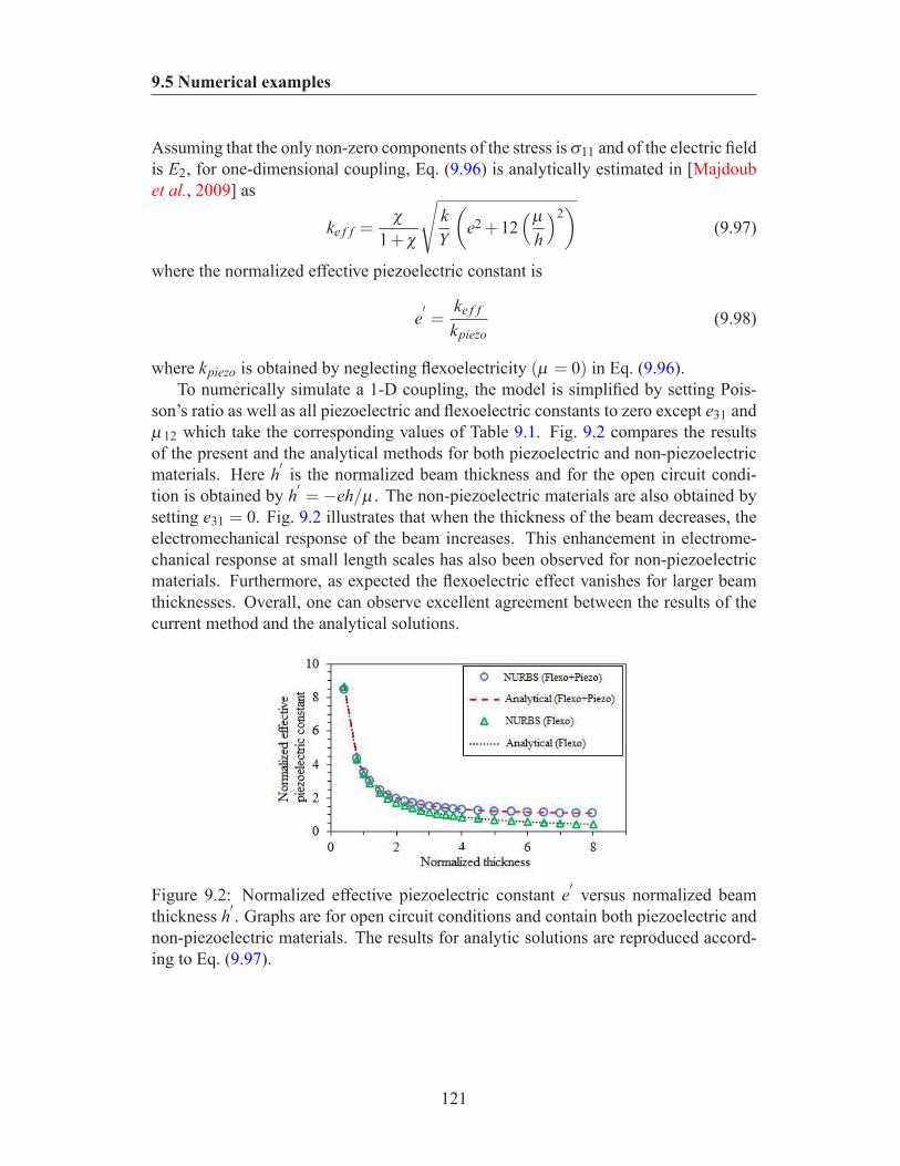
9.5 Numerical examples
Assuming that the only non-zero components of the stress is σ11 and of the electric fieldis E2, for one-dimensional coupling, Eq. (9.96) is analytically estimated in [Majdoubet al., 2009] as
ke f f =χ
1+χ
√kY
(e2 +12
(µh
)2)
(9.97)
where the normalized effective piezoelectric constant is
e′=
ke f fkpiezo
(9.98)
where kpiezo is obtained by neglecting flexoelectricity (µ = 0) in Eq. (9.96).To numerically simulate a 1-D coupling, the model is simplified by setting Pois-
son’s ratio as well as all piezoelectric and flexoelectric constants to zero except e31 andµ12 which take the corresponding values of Table 9.1. Fig. 9.2 compares the resultsof the present and the analytical methods for both piezoelectric and non-piezoelectricmaterials. Here h′ is the normalized beam thickness and for the open circuit condi-tion is obtained by h′
= −eh/µ . The non-piezoelectric materials are also obtained bysetting e31 = 0. Fig. 9.2 illustrates that when the thickness of the beam decreases, theelectromechanical response of the beam increases. This enhancement in electrome-chanical response at small length scales has also been observed for non-piezoelectricmaterials. Furthermore, as expected the flexoelectric effect vanishes for larger beamthicknesses. Overall, one can observe excellent agreement between the results of thecurrent method and the analytical solutions.
Figure 9.2: Normalized effective piezoelectric constant e′ versus normalized beamthickness h′ . Graphs are for open circuit conditions and contain both piezoelectric andnon-piezoelectric materials. The results for analytic solutions are reproduced accord-ing to Eq. (9.97).
121
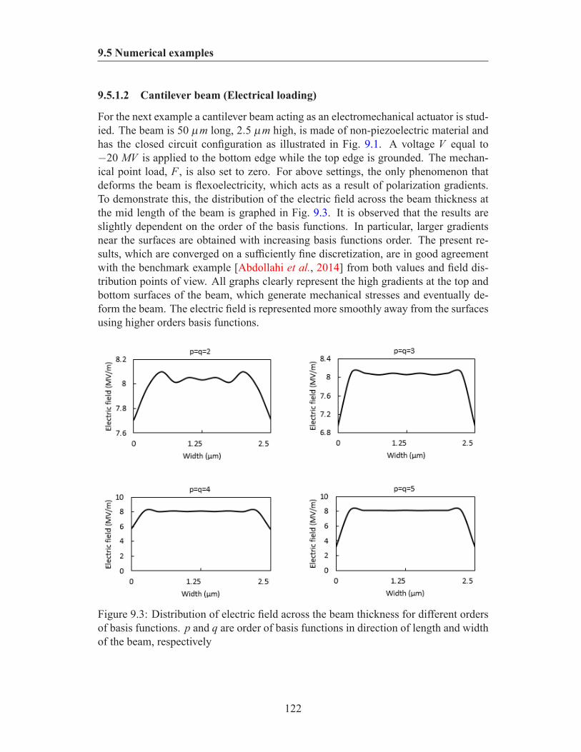
9.5 Numerical examples
9.5.1.2 Cantilever beam (Electrical loading)
For the next example a cantilever beam acting as an electromechanical actuator is stud-ied. The beam is 50 µm long, 2.5 µm high, is made of non-piezoelectric material andhas the closed circuit configuration as illustrated in Fig. 9.1. A voltage V equal to−20 MV is applied to the bottom edge while the top edge is grounded. The mechan-ical point load, F , is also set to zero. For above settings, the only phenomenon thatdeforms the beam is flexoelectricity, which acts as a result of polarization gradients.To demonstrate this, the distribution of the electric field across the beam thickness atthe mid length of the beam is graphed in Fig. 9.3. It is observed that the results areslightly dependent on the order of the basis functions. In particular, larger gradientsnear the surfaces are obtained with increasing basis functions order. The present re-sults, which are converged on a sufficiently fine discretization, are in good agreementwith the benchmark example [Abdollahi et al., 2014] from both values and field dis-tribution points of view. All graphs clearly represent the high gradients at the top andbottom surfaces of the beam, which generate mechanical stresses and eventually de-form the beam. The electric field is represented more smoothly away from the surfacesusing higher orders basis functions.
Figure 9.3: Distribution of electric field across the beam thickness for different ordersof basis functions. p and q are order of basis functions in direction of length and widthof the beam, respectively
122
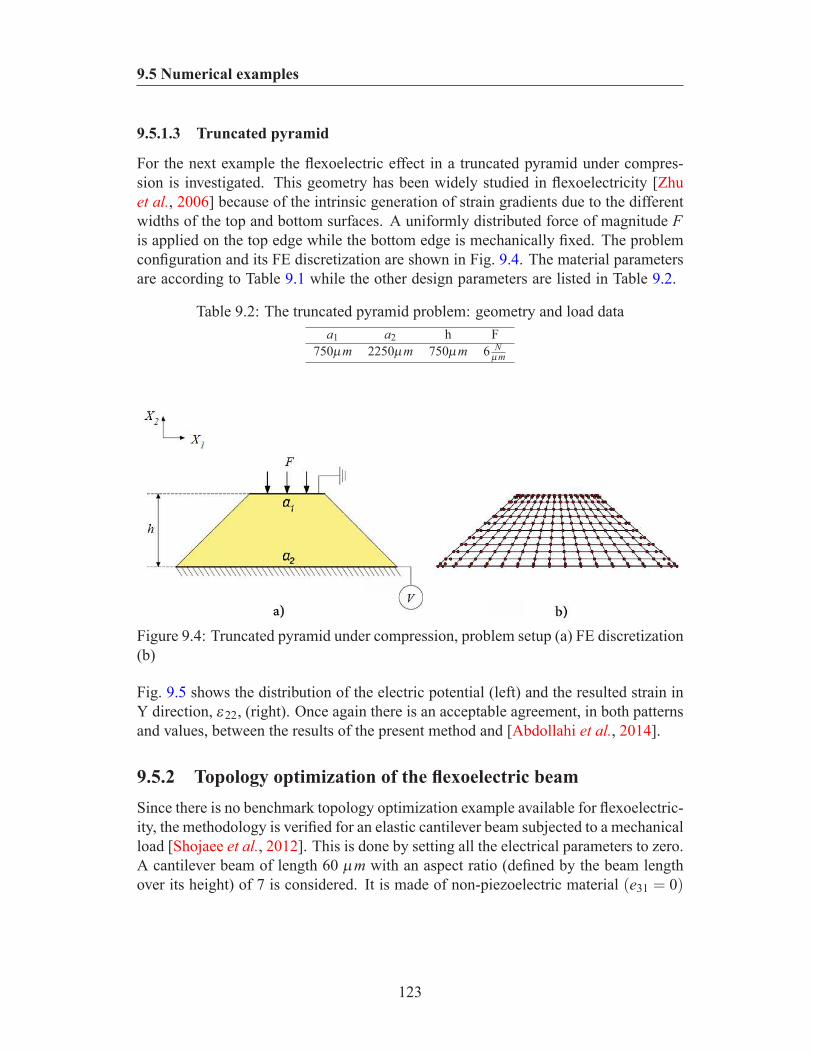
9.5 Numerical examples
9.5.1.3 Truncated pyramid
For the next example the flexoelectric effect in a truncated pyramid under compres-sion is investigated. This geometry has been widely studied in flexoelectricity [Zhuet al., 2006] because of the intrinsic generation of strain gradients due to the differentwidths of the top and bottom surfaces. A uniformly distributed force of magnitude Fis applied on the top edge while the bottom edge is mechanically fixed. The problemconfiguration and its FE discretization are shown in Fig. 9.4. The material parametersare according to Table 9.1 while the other design parameters are listed in Table 9.2.
Table 9.2: The truncated pyramid problem: geometry and load dataa1 a2 h F
750µm 2250µm 750µm 6 Nµm
Figure 9.4: Truncated pyramid under compression, problem setup (a) FE discretization(b)
Fig. 9.5 shows the distribution of the electric potential (left) and the resulted strain inY direction, ε22, (right). Once again there is an acceptable agreement, in both patternsand values, between the results of the present method and [Abdollahi et al., 2014].
9.5.2 Topology optimization of the flexoelectric beamSince there is no benchmark topology optimization example available for flexoelectric-ity, the methodology is verified for an elastic cantilever beam subjected to a mechanicalload [Shojaee et al., 2012]. This is done by setting all the electrical parameters to zero.A cantilever beam of length 60 µm with an aspect ratio (defined by the beam lengthover its height) of 7 is considered. It is made of non-piezoelectric material (e31 = 0)
123
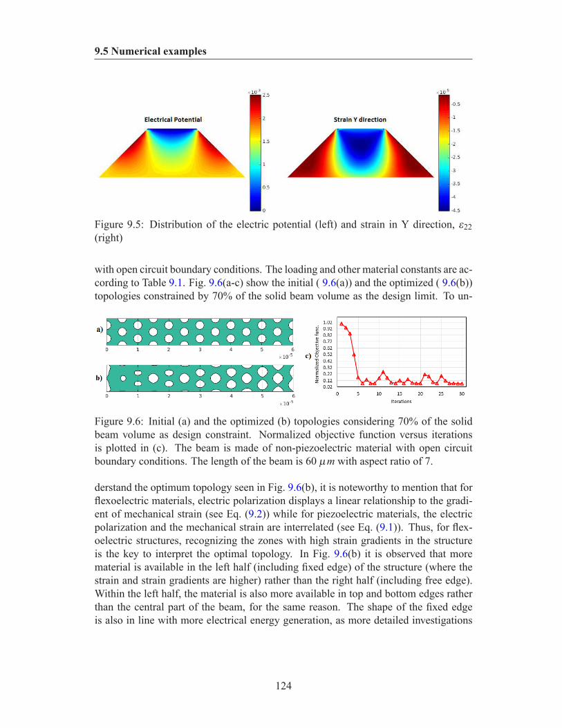
9.5 Numerical examples
Figure 9.5: Distribution of the electric potential (left) and strain in Y direction, ε22(right)
with open circuit boundary conditions. The loading and other material constants are ac-cording to Table 9.1. Fig. 9.6(a-c) show the initial ( 9.6(a)) and the optimized ( 9.6(b))topologies constrained by 70% of the solid beam volume as the design limit. To un-
Figure 9.6: Initial (a) and the optimized (b) topologies considering 70% of the solidbeam volume as design constraint. Normalized objective function versus iterationsis plotted in (c). The beam is made of non-piezoelectric material with open circuitboundary conditions. The length of the beam is 60 µm with aspect ratio of 7.
derstand the optimum topology seen in Fig. 9.6(b), it is noteworthy to mention that forflexoelectric materials, electric polarization displays a linear relationship to the gradi-ent of mechanical strain (see Eq. (9.2)) while for piezoelectric materials, the electricpolarization and the mechanical strain are interrelated (see Eq. (9.1)). Thus, for flex-oelectric structures, recognizing the zones with high strain gradients in the structureis the key to interpret the optimal topology. In Fig. 9.6(b) it is observed that morematerial is available in the left half (including fixed edge) of the structure (where thestrain and strain gradients are higher) rather than the right half (including free edge).Within the left half, the material is also more available in top and bottom edges ratherthan the central part of the beam, for the same reason. The shape of the fixed edgeis also in line with more electrical energy generation, as more detailed investigations
124
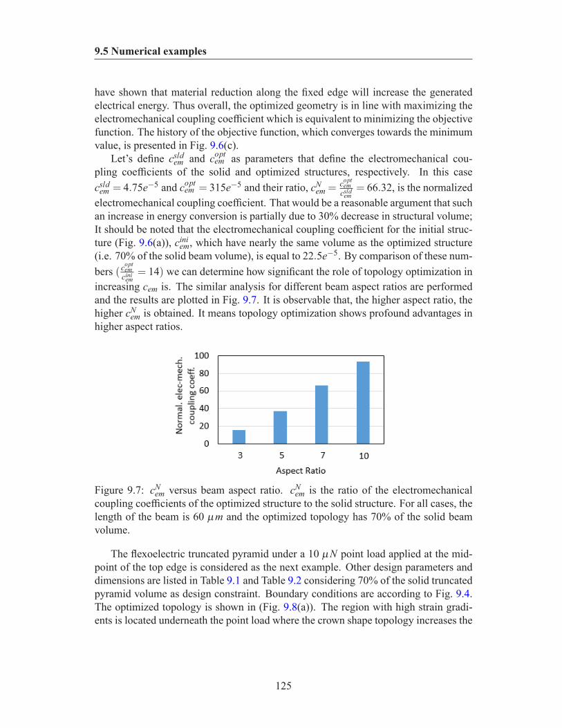
9.5 Numerical examples
have shown that material reduction along the fixed edge will increase the generatedelectrical energy. Thus overall, the optimized geometry is in line with maximizing theelectromechanical coupling coefficient which is equivalent to minimizing the objectivefunction. The history of the objective function, which converges towards the minimumvalue, is presented in Fig. 9.6(c).
Let’s define csldem and copt
em as parameters that define the electromechanical cou-pling coefficients of the solid and optimized structures, respectively. In this casecsld
em = 4.75e−5 and coptem = 315e−5 and their ratio, cN
em = coptem
csldem
= 66.32, is the normalizedelectromechanical coupling coefficient. That would be a reasonable argument that suchan increase in energy conversion is partially due to 30% decrease in structural volume;It should be noted that the electromechanical coupling coefficient for the initial struc-ture (Fig. 9.6(a)), cini
em, which have nearly the same volume as the optimized structure(i.e. 70% of the solid beam volume), is equal to 22.5e−5. By comparison of these num-bers (copt
emcini
em= 14) we can determine how significant the role of topology optimization in
increasing cem is. The similar analysis for different beam aspect ratios are performedand the results are plotted in Fig. 9.7. It is observable that, the higher aspect ratio, thehigher cN
em is obtained. It means topology optimization shows profound advantages inhigher aspect ratios.
Figure 9.7: cNem versus beam aspect ratio. cN
em is the ratio of the electromechanicalcoupling coefficients of the optimized structure to the solid structure. For all cases, thelength of the beam is 60 µm and the optimized topology has 70% of the solid beamvolume.
The flexoelectric truncated pyramid under a 10 µN point load applied at the mid-point of the top edge is considered as the next example. Other design parameters anddimensions are listed in Table 9.1 and Table 9.2 considering 70% of the solid truncatedpyramid volume as design constraint. Boundary conditions are according to Fig. 9.4.The optimized topology is shown in (Fig. 9.8(a)). The region with high strain gradi-ents is located underneath the point load where the crown shape topology increases the
125
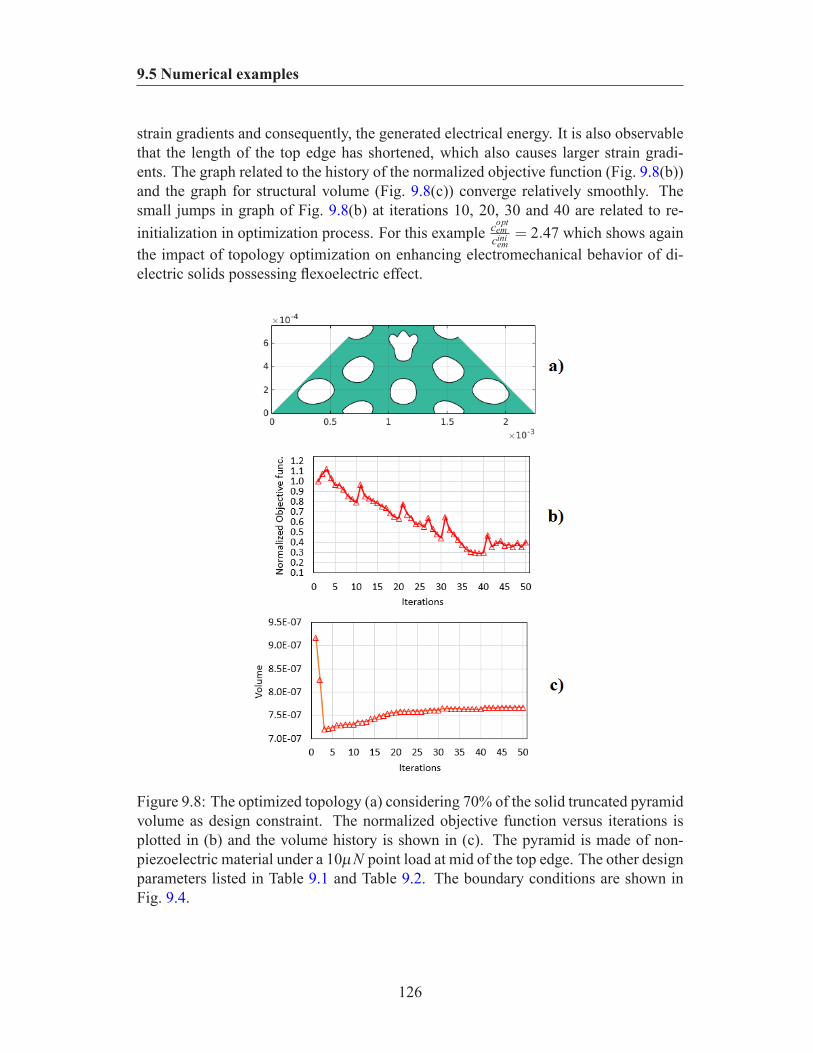
9.5 Numerical examples
strain gradients and consequently, the generated electrical energy. It is also observablethat the length of the top edge has shortened, which also causes larger strain gradi-ents. The graph related to the history of the normalized objective function (Fig. 9.8(b))and the graph for structural volume (Fig. 9.8(c)) converge relatively smoothly. Thesmall jumps in graph of Fig. 9.8(b) at iterations 10, 20, 30 and 40 are related to re-initialization in optimization process. For this example copt
emcini
em= 2.47 which shows again
the impact of topology optimization on enhancing electromechanical behavior of di-electric solids possessing flexoelectric effect.
Figure 9.8: The optimized topology (a) considering 70% of the solid truncated pyramidvolume as design constraint. The normalized objective function versus iterations isplotted in (b) and the volume history is shown in (c). The pyramid is made of non-piezoelectric material under a 10µN point load at mid of the top edge. The other designparameters listed in Table 9.1 and Table 9.2. The boundary conditions are shown inFig. 9.4.
126
9.6 Concluding remarks
9.6 Concluding remarksA computational framework for topology optimization of flexoelectric micro and nanos-tructures is presented to enhance their energy conversion efficiency. The methodologyis based on a combination of isogeometric analysis (IGA), level set and point wisedensity mapping techniques. The smoothness of the IGA basis functions is used todiscretize the fourth order partial differential equations of flexoelectricity, while thelevel set provide clear boundaries and gives stable convergence. The point wise den-sity mapping is directly used in the weak form of the governing equations and itsderivative can be consistently derived. The nodal level set values on control pointsand the inverse of the electromechanical coupling coefficient are defined as designvariables and objective function, respectively. The numerical results demonstrate thatB-spline elements can successfully model the flexoelectric effect in dielectrics. For acantilever beam with constant length, it is shown that when the thickness of the beamdecreases, the electromechanical response increases. The topology optimization is alsoable to noticeably increase the electromechanical coupling coefficient, with substantialenhancements observed for higher aspect ratios.
127
Chapter 10
Conclusions
10.1 Summary of achievementsThe methodology and achievements of this research work are highlighted within fol-lowing four items:
1. Fiber distribution optimization:An efficient gradient based computational technique for fiber distribution opti-mization in fiber reinforced continuum elements, has been developed throughthe use of Non-Uniform Rational B-spline (NURBS) functions. Nodal volumefraction of fiber has been used as the optimization design variable, whose dis-tribution function has been smoothly approximated by using a NURBS surface.The methodology allows considering different material models and generic ob-jective functions. The main advantage of the proposed approach is that domaindiscretization and definition of fiber distribution function have common data sets.It also allows to get a high rate and smooth convergence to the optimum conditionsought.
2. Uncertainties propagation:Deterministic approaches for nanocomposite modeling and optimization mightbe unrealistic for certain applications and may yield to either catastrophic failureor unnecessary conservatism. Detailed investigations on uncertainties and theirpropagation have been performed for obtaining realistic and reliable PolymericNano Composite (PNC) structures. Potential uncertainties have been categorizedin material, structural and modeling levels. To fully address uncertainties in ma-terial level, a stochastic multi-scale material model (which includes all importantaspects of the Carbon Nano Tube Reinforced Polymer (CNTRP) including CNTlength, orientation, dispersion, agglomeration and waviness, at different lengthscales from nano-, up to macro-scale) has been utilized. To improve the compu-
128

10.1 Summary of achievements
tational efficiency, the evaluation of material properties has been surrogated by ametamodel. The results for two selected examples show that the failure probabil-ity of a polymeric nanocomposite structure, strongly depends on the CNT param-eters, especially the CNT volume fraction and the waviness. The influence of theCNT agglomeration is nearly negligible. It was observed that neglecting the CNTagglomeration can simplify the model and decrease the computational time with-out remarkable loss in model accuracy. Furthermore, the loading condition anddiscretization affect the reliability of the system. Coarse meshes underestimatethe failure probability of a beam while fine meshes admittedly increase computa-tional cost. Thus sufficiently refined discretization should be investigated in orderto have realistic assessment of the reliability of PNC structures. An increase inthe standard deviation of the applied load, which physically means more uncer-tainties in the system, resulted in the structure with a smaller reliability index.Finding the optimal content of CNT was also presented to optimized the materialinstead of the geometry. As a further step forward, concurrent optimization ofmaterial parameters and geometrical parameters (hybrid optimization) was con-ducted to present a comprehensive solution for current demands in fully opti-mized designs of nanocomposite components.
3. Sequential optimization approach:The two previous items are integrated resulted in an efficient sequential algo-rithm for finding the optimal fiber volume fraction and its distribution in struc-tures made of Fiber Reinforced Composite (FRC) materials. To overcome thecumbersome computational burden in stochastic optimization problems, findingthe optimal fiber volume fraction and fiber distribution are performed sequen-tially, not concurrently. This technique along with using NURBS finite elements,allows us to get a noticeable reduction in the computational cost, without a no-ticeable loss in accuracy of the results. Assuming a (simplified energy-basedmaterial model) random orientation of fibers in the matrix, in the first optimiza-tion module (i.e. finding the optimal fiber volume fraction) uncertainties in theparameters (such as constituents materials and loading) are fully addressed andLimit State Function (LSF) is evaluated by using First Order Reliability Method(FORM). In the second module (i.e. fiber distribution optimization) a NURBSsurface which smoothly defines the fiber distribution pattern, is adopted. Thepresented numerical examples show as an increase in model uncertainties givesrise to unreliability of the system. More specifically, either the rise in the num-ber of uncertain fields in the problem or the increase in the standard deviation ofrandom variables needs more fiber content. It can be also concluded that whenthere is a higher level of uncertainties in design parameters, the fiber distributionoptimization is more influential on increasing the reliability of the structure.
4. Innovative applications:
129
10.1 Summary of achievements
The methodology is applied in three novel applications with following achieve-ments / observations:
• Interfacial shear stress optimization in sandwich beams:A computational algorithm for decreasing interfacial shear stress in sand-wich beams with polymeric core is presented. The algorithm can be alsoused for optimizing other stress components (i.e. peeling and bending stresses)in any arbitrary zone of the design domain. C−1 continuity is imposed at theinterface to ”truly” isolate the reinforcement distribution in the core from theface sheets using multi-patch and penalty techniques. Comparing the resultsof the case study illustrates that adding reinforcements homogeneously intopolymers will slightly improve the interfacial shear stress but that consider-able improvements are observed when the distribution of the reinforcementin the core is optimized.
• Probabilistic multiconstraints optimization of cooling channels in CeramicMatrix Composites (CMC):The presented computational platform efficiently optimizes the capacity ofcooling channels in a components made of CMC using Reliability Based De-sign Optimization (RBDO) approach. A ”series system” reliability conceptis adopted as a union of mechanical and thermal failure subsets. Afterwards,the optimizer is supposed to increase the reliability of the component by op-timally distributing the C-fibers inside the matrix within the design domain.Numerical results for the performed case studies demonstrate that optimaldistribution of C-fibers can decrease structural and thermal compliances. Inthe decoupled elastic and thermal problems, the former yields an increase inβm (the reliability index associated with the probabilistic deformation con-straint) and the latter in an increase in βt (the reliability index associatedwith the probabilistic thermal constraint). But, in the coupled thermoelasticproblem, any prediction about final reliability indices depends on fiber andmatrix constitutive material properties and contribution of mechanical andthermal loadings on the global force vector. When the mechanical loadingdominates the thermal loading, fiber distribution can show promising advan-tage to have more reliable design by increasing βm and consequently βtarget(the final reliability index). However, its role for increasing the reliabilityindex corresponding to thermal constraint is negligible.
• Topology optimization of flexoelectric materials:A computational framework for topology optimization of flexoelectric mi-cro and nanostructures is presented to enhance their energy conversion effi-ciency. The methodology is based on a combination of isogeometric analysis(IGA), level set and point wise density mapping techniques. The smoothnessof the IGA basis functions is used to discretize the fourth order partial differ-
130
10.2 Outlook
ential equations of flexoelectricity, while the level set provide clear bound-aries and gives stable convergence. The point wise density mapping is di-rectly used in the weak form of the governing equations and its derivative canbe consistently derived. The nodal level set values on control points and theinverse of the electromechanical coupling coefficient are defined as designvariables and objective function, respectively. The numerical results demon-strate that B-spline elements can successfully model the flexoelectric effectin dielectrics. For a cantilever beam with constant length, it is shown thatwhen the thickness of the beam decreases, the electromechanical responseincreases. The topology optimization is also able to noticeably increase theelectromechanical coupling coefficient, with substantial enhancements ob-served for higher aspect ratios.
10.2 OutlookThe presented work established the framework for probabilistic optimization of fiberreinforced composites with some promising applications. It is also extended and usedas a topology optimization tool for flexoelectric micro-nano devices. A few possibleextensions to the current work can be suggested as follows:
• Extend the methodology to 3-D to be able to address more general problems• Investigate different failure criteria as limit state functions• Contributing the developed methodology towards the design of micro and nano-
scale energy harvesters / sensors with optimized electromechanical performance• Addressing the available uncertainties in optimization of micro-nano electrome-
chanical devices• Contributing towards the design of multi-material micro and nano-scale energy
harvesters / sensors
131
Bibliography
Abdollahi, Amir, Peco, Christian, Millan, Daniel, Arroyo, Marino, & Arias, Irene.2014. Computational evaluation of the flexoelectric effect in dielectric solids.JOURNAL OF APPLIED PHYSICS, 116, 093502. 108, 109, 120, 122, 123
Abdollahi, Amir, Millan, Daniel, Peco, Christian, Arroyo, Marino, & Arias, Irene.2015. Revisiting pyramid compression to quantify flexoelectricity: A three-dimensional simulation study. PHYSICAL REVIEW B, 91, 104103. 108
Ahmadpour, F., & Sharma, P. 2015. Flexoelectricity in two-dimensional crystallineand biological membranes. nanoscale, 7, 16555–16570. 107
Almeida, F.S., & Awruch, A.M. 2009. Design optimization of composite laminatedstructures using genetic algorithms and finite element analysis. Compos. Struct., 88,443–454. 3
Antonio, C. C., & Hoffbauer, L. N. 2009. An approach for reliability-based robustdesign optimization of angle-ply composites. Compos. Struct., 90, 53–59. 4
Apalak, M. Kemal, & Yildirim, Mustafa. 2008. Layer optimization for maximumfundamental frequency of laminated composite plates for different edge conditions.Compos. Struct., 68, 537–550. 3
Bendse, M. P., & Kikuchi, N. 1988. Generating Optimal Topologies in StructuralDesign using a Homogenization Method. Computer Methods in Applied Mechanicsand Engineering, 71. 108
Bendsoe, MP., & Sigmund, O. 2003. Topology optimization:Theory, Methods, andApplications. Germany: Springer. 72
Bourinet, J.-M. 2010. FERUM 4.1 user’s guide. available online at:http://www.ifma.fr/cache/offonce/lang. 16, 42, 92
132
BIBLIOGRAPHY
Brighenti, R. 2004a. A mechanical model for fiber reinforced composite materialswith elasto-plastic matrix and interface debonding. Int. J. Comput. Mater. Sci., 29,475–493. 18, 19
Brighenti, R. 2004b. Numerical modeling of the fatigue behavior of fiber-reinforcedcomposites. Int. J. Compos. B: Eng., 35. 19
Brighenti, R. 2004c. Optimum patch repair shapes for cracked members. Int. J. Mech.Mater. Des., 1. 3
Brighenti, R. 2005. Fiber distribution optimization in fiber-reinforced composites by agenetic algorithm. Compos. Struct., 71, 1–15. viii, 2, 3, 17, 27, 28
Brighenti, R. 2007. Patch repair design optimization for fracture and fatigue improve-ments of cracked plates. J. Sol. Struct., 44. 3
Brighenti, R. 2012. A micromechanical model and reinforcing distribution optimiza-tion approach for fiber-reinforced materials. In: Qingzheng (George) Cheng (ed)Fiber Reinforced Composites. Hauppauge, NY: Nova Science Publishers, Inc. viii,19, 20
Brighenti, R., & Scorza, D. 2012. A micro-mechanical model for statistically unidi-rectional and randomly distributed fiber-reinforced solids. Math. Mech. Solids, 17.21
Brighenti, R., Carpinteri, A., & Vantadori, S.A. 2006. genetic algorithm applied tooptimization of patch repairs for cracked plates. Comp. Meth. App. Mech. Eng.,1960, 466–475. 3
Bui, TQ., Kosravifard, A., Zhang, CH., Hematiyan, Mr., & Golub, MV. 2013. Dynamicanalysis of sandwich beam with functionally graded core using a truly meshfreeradial point interpolation method. Eng. struct., 47, 90–104. x, 66, 67, 77
Cai, Y., Zhuang, X., & Zhu, H. 2013. A generalized and efficient method for finitecover generation in the numerical manifold method. Int. J. of Comput. Methods, 10.68
Chiachio, M., Chiachio, J., & Rus, G. 2012. Reliability in composites - A selectivereview and survey of current development. Composites, 43. 14
Cottrell, J.A., Hughes, T.J.R., & Bazilevs, Y. 2009. Isogeometric Analysis towardsintegration of CAD and FEA. UK: Wiley. 8, 9, 10, 71
133
BIBLIOGRAPHY
Dennis, B., Egorov, I., Dulikravich, G., & Yoshimura, S. 2003. Optimization of alarge number of coolant passages located close to the surface of a turbine blade. In:Proceedings of ASME Turbo Expo 2003, Power for Land, Sea and Air Conference.Atlanta, Georgia, June 16-19. 86
Ditlevsen, O., & Madsen, H. 1996. Structural reliability methods. UK: John WileySons. 12
Du, J., & Olhoff, N. 2007. Topological design for freely vibrating continuum structuresfor maximum values of simple and multiple eigenfrequencies and frequency gaps.Struct. Multidisc. Opt., 34, 91–110. 21
Duddu, R., Bordas, SPA., Chopp, D., & Moran, B. 2008. A combined extended finiteelement and level set method for biofilm growth. Int. J. Numer. Meth. Engng., 74.68
Ghorashi, SS., Valizadeh, N., & Mohammadi, S. 2012. Extended isogeometric analysisfor simulation of stationary and propagating cracks. Int. J. Numer. Meth. Engng., 89,1069–1101. 68
Gomes, H.M., & Awruch, A.M. 2011. Reliability based optimization of lami-nated composite structures using genetic algorithms and Artificial Neural Networks.Struct. saf., 33, 186–195. 4
Hashin, Z. 1962. The elastic moduli of heterogeneous materials. J Appl. Mech., 29,143–150. 18
Hashin, Z., & Shtrikman, S. 1963. A variational approach to the theory of elasticbehavior of multiphase materials. J. Mech. Phys. Solids, 11, 127–140. 18
Hasofer, A.M., & Lind, N. 1974. An Exact and Invariant First-Order Reliability For-mat. J. Eng. Mech. ASCE, 100, 111–121. 12
Hill, R. 1965. A self-consistent mechanics of composite materials. J. Mech. Phys.Solids, 13, 213–222. 18
Honda, Shinya, & Narita, Yoshihiro. 2011. Vibration design of laminated fibrous com-posite plates with local anisotropy induced by short fibers and curvilinear fibers.Compos. Struct., 93, 902–910. 3
Hu, H., Belouettar, S., Ferry, MP., & Daya, EM. 2008. Review and assessment ofvarious theories for modeling sandwich composites. Compos. Struct., 84, 282–292.65
134
BIBLIOGRAPHY
Huang, J., & Haftka, R.T. 2005. Optimization of fiber orientations near a hole forincreased load-carrying capacity of composite laminates. Struct. Multidisc. Optim.,30, 335–341. 3
Hughes, TJR., Cottrell, JA., & Bazilevs, Y. 2005. Isogeometric Analysis: CAD, finiteelements, NURBS, exact geometry and mesh refinement. Comput. Methods Appl.Mech. Eng., 194, 4135–4195. 8
Jha, DK., Kant, T., & Singh, RK. 2013. A critical review of recent research on func-tionally graded plates. Compos. Struct., 96, 833–849. 65
Jia, Y., Anitescu, C., Ghorashi, SS., & Rabczuk, T. 2014. Extended isogeometricanalysis for material interface problems. IMA J. of Appl. Math. 68
Jiang, C., Han, X., & Liu, G.P. 2008. Uncertain optimization of composite laminatedplates using a nonlinear interval number programming method. Comput. and struct.,86, 1696–1703. 4
Kim, Taeseong, & Lim, Jaehoon. 2013. Structural design optimization of a tiltrotoraircraft composite wing to enhance whirl flutter stability. Compos. Struct., 95, 283–294. 3
Krenkel, W. 2005. Carbon fiber reinforced Silicon Carbide composites (C/SIC, C/C-SIC). In: Bansal Narottam P, editor. Hand book of ceramic composites. US:Springer. 86
Krour, B., Bernard, F., & Tounsi, A. 2013. Fibers orientation optimization for con-crete beam strengthened with a CFRP bonded plate: A coupled analyticalnumericalinvestigation. Eng. struct., 56, 218–227. 65
Kulasegaram, S., & Karihaloo, B.L. 2012. Fibre-reinforced, self-compacting concreteflow modelled by smooth particle hydrodynamics. Proc. ICE Eng. Comput. Mech.,166. 3
Kulasegaram, S., Karihaloo, B.L., & Ghanbari, A. 2011. Modelling the flow of self-compacting concrete, International Journal for Numerical and Analytical Methodsin Geomechanics. Int. J. Numer. Anal. Meth. Geomech., 35. 3
Lau, K.T., Gu, C., & Hui, D. 2006. A critical review on nanotube and nan-otube/nanoclay related polymer composite materials. Compos: Part B-Eng., 37,425–436. 35
Lee, D.S., & Morillo, C. 2012. Multilayered composite structure design optimizationusing distributed/parallel multi-objective evolutionary algorithms. Compos. Struct.,94, 1087–1096. 3
135
BIBLIOGRAPHY
Lee, Gyeong-Chan, & Kweon, Jin-Hwe. 2013. Optimization of composite sandwichcylinders for underwater vehicle application. Compos. Struct., 96, 691–697. 3
Liu, GR., Wang, Z., Zhang, GY., Zong, Z., & Wang, S. 2012. An Edge-BasedSmoothed Point Interpolation Method for Material Discontinuity. Mech. of Adv.Mater. and Struct., 19. 76
Logan, DL. 2007. A first course in the finite element method. CA: Nelson. 90
Lophaven, S.N., Nielsen, H.B., & Sondergaard, J. 2002. DACE a Matlab kriging tool-box version 2.0, Technical Report IMM-TR-2002-12. Informatics and mathematicalmodeling. 39, 41
Lousdad, A., Megueni, A., & Bouchikhi, AS. 2010. Geometric edge shape basedoptimization for interfacial shear stress reduction in fiber reinforced polymer plateretrofitted concrete beams. Comput. mat. sci., 47, 911–918. 65
Majdoub, M. S., Sharma, P., & Cagin, T. 2009. Enhanced size-dependent piezoelec-tricity and elasticity in nanostructures due to the flexoelectric effect. PHYSICALREVIEW B, 79, 119904 (E). 108, 114, 121
Manalo, AC, Aravinthan, T., & Karunasena, W. 2009. Flexural behavior of laminatedfiber composite sandwich beams. Proceedings of the second official internationalconference of international institute for FRP in construction for Asia-Pacific region,Seoul, 407–412. 65
Marler, R.T., & Arora, J.S. 2004. Survay of multi-objective optimization methods forengineering. Struct. Multidisc. Opt., 26, 369–395. 21
Mashkevich, V. S., & Tolpygo, K. B. 1957. Electrical, optical and elastic properties ofdiamond crystals. Soviet Physics, 5. 107
Mori, T., & Tanaka, K. 1973. Average stress in matrix and average elastic energy ofmaterials with mis-fitting inclusions. Acta Metal, 21, 571–583. 18, 38, 66, 67
Murugan, Senthil, & Flores, Erick I. Saavedra. 2012. Optimal design of variable fiberspacing composites for morphing aircraft skins. Compos. Struct., 94, 1626–1633. 3
Nadeau, J.C., & Ferrari, M. 1999. Microstructural optimization of a functionallygraded transversely isotropic layer. Mechanics of Materials, 31, 637–651. 3
Nagaiah, NR:, & Geiger, CD. 2014. Evolutionary numerical simulation approach fordesign optimization of gas turbine blade cooling channels. Int. J. Simul. Multisci.Des. Optim., 5, A22. 86
136
BIBLIOGRAPHY
Nanthakumar, S., Lahmer, T., & Rabczuk, T. 2013. Detection of flaws in piezoelectricstructures using XFEM. International Journal of Numerical Methods in Engineer-ing, 96. 107
Nanthakumar, S., Lahmer, T., & Rabczuk, T. 2014. Detection of multiple flaws inpiezoelectric structures using XFEM and Level sets. Computer Methods in AppliedMechanics and Engineering, 275, 98–112. 107
Nanthakumar, S., Valizadeh, N., Park, Harold S., & Rabczuk, T. 2015. Surface effectson shape and topology optimization of nanostructures. Comput Mech, 56, 97–112.108
Nanthakumar, S., Lahmer, T., Zhuang, X., Zi, G., & Rabczuk, T. 2016. Detection ofmaterial interfaces using a regularized level set method in piezoelectric structures.Inverse Problems in Science and Engineering, 24. 107
Nguyen, T. D., Mao, S., Yeh, Y-W, Purohit, P. K., & McAlpine, M. C. 2013. Nanoscaleflexoelectricity. Adv. Mater., 25, 946–74. 108
Nguyen, VP., Kerfriden, P., & Bordas, SPA. 2014. Two- and three-dimensional iso-geometric cohesive elements for composite delamination analysis. Compos. Part B:Eng., 60, 193–212. 68
Nguyen, VP., Anitescu, Cosmin, Rabczuk, T., & Bordas, SPA. 2015. Isogeometricanalysis: An overview and computer implementation aspects. Math. and Comput.in Simul., 117, 89–116. 76
Nikolaidis, E., Ghiocel, DM., & Singhal, S. 2005. Engineering design reliability hand-book. US: CRC Press. 91, 92
Noh, Y.J., & Kang., Y.J. 2013. Reliability-based design optimization of volume frac-tion distribution in functionally graded composites. Comp. Mater. Sci., 69, 435–442.4
Omkar, S.N., & Mudigere, Dheevatsa. 2008. Vector evaluated particle swarm opti-mization (VEPSO) for multi-objective design optimization of composite structures.Comput. Struct., 86, 1–14. 3
Osher, S., & Sethian, J.A. 1988. Front propagating with curvature dependent speed:algorithms based on Hamilton-jacobi formulations. J. Comp. Physics, 78, 12–49.108
Park, Hong-Seok, & Dang, Xuan-Phuong. 2010. Structural optimization based onCAD-CAE integration and metamodeling techniques. Comput. Aided Des., 42, 889–902. 39
137
BIBLIOGRAPHY
Paul, B. 1960. Prediction of elastic constants of multiphase materials. Trans. Metall.Soc. AIME, 36–41. 18
Rabczuk, T., & Belytschko, T. 2004. Particles: a simplified meshfree method forarbitrary evolving cracks. Int. J. Numer. Meth. Engng., 61, 2316–2343. 68
Rabczuk, T., & Belytschko, T. 2007. A three-dimensional large deformation meshfreemethod for arbitrary evolving cracks. Comput. Methods Appl. Mech. Eng., 196,2777–2799. 68
Rabczuk, T., Areias, P., & Belytschko, T. 2007. A meshfree thin shell method fornon-linear dynamic fracture. Int. J. Numer. Meth. Engng., 72. 68
Rouhi, M., & Rais-Rohani, M. 2013. Modeling and probabilistic design optimizationof a nanofiber-enhanced composite cylinder for buckling. Compos. Struct., 95, 346–353. 4, 36, 44, 45
Rozvany, GIN, Zhou, M., & Birker, T. 1992. Generalized shape optimization withouthomogenization. Struct Multidisc Optim, 4, 250254. 108
Salzar, R.S. 1995. Functionaly graded metal matrix composite tubes. Compos. Eng.,5, 891–900. 3
Sharma, N.D., Maranganti, R., & Sharma, P. 2007. On the possibility of piezoelectricnanocomposites without using piezoelectric materials. Journal of the Mechanicsand Physics of Solids, 55, 23282350. 107, 108, 114
Sharma, N.D., Landis, C.M., & Sharma, P. 2010. Piezoelectric thin-film super-latticeswithout using piezoelectric materials. J. Appl. Phys., 108, 024304. 108
Shi, D.L., Feng, X.Q., Huang, Y.Y., Hwang, K.C., & Gao, H. 2004. The Effect of Nan-otube Waviness and Agglomeration on the Elastic Property of Carbon Nanotube-Reinforced Composites. J. Eng. Mater. Technol, 126. 38
Shojaee, S., Mohamadian, M., & Valizadeh, N. 2012. Composition of isogeometricanalysis with level set method for structural topology optimization. Int. J. Optim.Civil Eng., 2. 123
Shokrieh, M.M., & Rafiee, R. 2010a. Investigation of nanotube length effect on thereinforcement efficiency in carbon nanotube based composites. Compos. Struct., 92,2415–2420. 36
Shokrieh, M.M., & Rafiee, R. 2010b. Prediction of mechanical properties of an em-bedded carbon nanotube in polymer matrix based on developing an equivalent longfiber. Mech. Res. Commun., 37, 235–240. 36, 38
138
BIBLIOGRAPHY
Shokrieh, M.M., & Rafiee, R. 2010c. A review of the mechanical properties of isolatedcarbon nanotubes and carbon nanotube composites. Mech. Compos. Mater., 46. 4,35, 36
Shokrieh, M.M., & Rafiee, R. 2010d. Stochastic multi-scale modeling ofCNT/polymer composites. Comput. Mater. Sci., 50. ix, 36, 38, 39, 40, 44
Shokrieh, M.M., & Rafiee, R. 2012. Development of a full range multi-scale model toobtain elastic properties of CNT/polymer composites. Iranian Polym. J., 21, 397–402. 35
Sigmund, Ole. 1997. On the Design of Compliant Mechanisms Using Topology Opti-mization. Mech. Struct. Mach., 25. 108
Sigmund, Ole. 2001a. A 99 line topology optimization code written in Matlab. Struc-tural and Multidisciplinary Optimization, 21. 108
Sigmund, Ole. 2001b. Design of multiphysics actuators using topology optimizationPart I: One material structures. Comput. Methods Appl. Mech. Engrg., 190, 6577–6604. 108
Svanberg, K. 1987. The method of moving asymptotes- a new method for structuraloptimization. Int. J. Numer. Meth. Eng., 24, 359–373. 23
Thanedar, P.B., & Chamis, C.C. 1995. Reliability considerations in composite lami-nates tailoring. Comput. and struct., 54. 4
Togan, V., & Daloglu, A. 2006. Reliability and reliability based design optimization.Turkish J. Eng. Env. Sci., 30, 237–249. 58
Triantafillou, TC., & Gibson, LJ. 1989. Debonding in foam-core sandwich panels.Mater. and Struct., 22, 64–69. 65
Wang, Michael Yu, Wang, Xiaoming, & Guo, Dongming. 2003. A level set methodfor structural topology optimization. Comput. Methods Appl. Mech. Engrg., 192,227–246. 108, 115, 116
Wu, SC., Liu, GR., Zhang, HO., & Zhang, GY. 2009. A node-based smoothed pointinterpolation method (NS-PIM) for thermoelastic problems with solution bounds.International Journal of Heat and Mass Transfer, 52, 1464–1471. 87
Yudin, P. V., & Tagantsev, A. K. 2013. TOPICAL REVIEW: Fundamentals of flexo-electricity in solids. Nanotechnology, 24, 36pp. 107
139
BIBLIOGRAPHY
Zehnder, N., & Ermanni, P. 2006. A methodology for the global optimization of lami-nated composite structures. Compos. Struct., 72, 311–320. 3
Zhao, X., Bordas, SPA., & Qu, J. 2013. A hybrid smoothed extended finite ele-ment/level set method for modeling equilibrium shapes of nano-inhomogeneities.Comput Mech., 52, 1417–1428. 68
Zhao, Yan-Gang, & Ono, Tetsuro. 1999. A general procedure for first/second-orderreliability method (FORM/SORM). Struct. Saf., 21, 95–112. 14
Zhou, M., & Rozvany, G.I.N. 1991. The COC algorithm part II: topological, geometryand generalized shape optimization. Comput. Meth. Appl. Mech. Eng., 89, 197–224.23, 71
Zhu, W.Y., Fu, J.Y., Li, N., & Cross, L. 2006. Piezoelectric composite based on theenhanced flexoelectric effects. Applied Physics Letters, 89, 192904. 123
Zhuang, X., Augarde, C., & Mathisen, K. 2012. Fracture modeling using meshlessmethods and level sets in 3D: framework and modeling. Int. J. Numer. Meth. Engng.,92, 969–998. 68
Zong, Z., Lam, KY, & Zhang, YY. 2005. The multidomain differential quadratureapproach to plane elastic problems with material discontinuity. Math. and comput.model., 41, 539–553. 74
Zubko, P., Catalan, G., & Tagantsev, A. K. 2013. Flexoelectric effect in solids. Annu.Rev. Mater. Res., 43, 38742. 108
140
Academic Curriculum Vitae
Hamid Ghasemi MeyghaniInstitute of Structural MechanicsBauhaus-Universitat WeimarMarienstrasse 15, 99423 Weimar, GermanyEmail: [email protected] of Birth: June 06th,1981Place of Birth: Arak, IranCitizenship: Iranian
Education• Ph.D: Computational Mechanics, Institute of Structural Mechanics, Bauhaus-
Universitat Weimar, Germany, 2012-2016.• M.Sc: Mechanical Engineering, Iran University of Science and Tech-
nology, Tehran, Iran 2004-2006• B.S: Mechanical Engineering, Tabriz University, Tabtiz, Iran 1999-
2003
Publications1. Hamid Ghasemi, Harold park, Timon Rabczuk A level-set based IGA
formulation for topology optimization of flexoelectric materials. Com-put. Methods Appl. Mech. Engrg. 313: 239-258, 2017
2. Hamid Ghasemi, Pierre Kerfriden, Stephane P. A. Bordas, Jacob Muthu,Goangseup Zi, Timon Rabczuk Probabilistic multiconstraints optimiza-tion of cooling channels in ceramic matrix composites. CompositesPart B 81:107-119, 2015
3. H. Ghasemi, R. Brighenti, X. Zhuang, J. Muthu, T. Rabczuk Optimumfiber content and distribution in fiber-reinforced solids using a relia-bility and NURBS based sequential optimization approach. Structuraland Multidisciplinary Optimization 51(1):99-112, 2015
4. Hamid Ghasemi, Pierre Kerfriden, Stephane P. A. Bordas, Jacob Muthu,Goangseup Zi, Timon Rabczuk Interfacial shear stress optimization in

sandwich beams with polymeric core using non-uniform distribution ofreinforcing ingredients. Composite Structures 120:221-230, 2015
5. H. Ghasemi, R. Brighenti, X. Zhuang, J. Muthu, T. Rabczuk Optimiza-tion of fiber distribution in fiber reinforced composite by using NURBSfunctions. Computational Material Science 83: 463473, 2014
6. H. Ghasemi, Roham Rafiee, X. Zhuang, J. Muthu, T. Rabczuk Uncer-tainties propagation in metamodel-based probabilistic optimization ofCNT/polymer composite structure using stochastic multi-scale model-ing. Computational Material Science 85: 295-305, 2014


![Springer MRW: [AU:, IDX:] · Generally, hybrids have better properties than single-fiber composites and are more costly. The composites are called a hybrid when more than one type](https://img.pdfslide.us/doc/110x75/5f2f551e4e161c5ac3375731/springer-mrw-au-idx-generally-hybrids-have-better-properties-than-single-iber.jpg)