STOCHASTIC MODELS FOR ACTUARIAL USE:

THE EQUILIBRIUM MODELLING OF LOCAL MARKETS

Rob Thomson, Dmitri Gott

Hacettepe University

24th June 2011

2

Agenda

Introduction Assumptions Prices and returns Notional risky assets Development of the model Summary of the model Parameter estimation Illustrative results

3

Introduction

Predictive model of returns on the market portfolio Predictive equilibrium model of:

(real) returns on major asset categories(real) risk-free rates inflation rates(interdependent) factors(independent) notional risky assets

Descriptive estimation of the equilibrium model

4

Agenda

Introduction Assumptions Prices and returns Notional risky assets Development of the model Summary of the model Parameter estimation Illustrative results

5

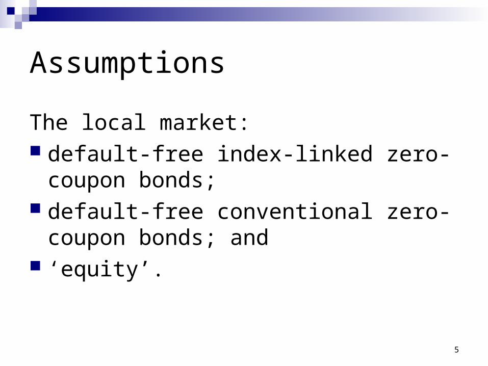
Assumptions

The local market: default-free index-linked zero-coupon bonds; default-free conventional zero-coupon bonds;

and ‘equity’.

6

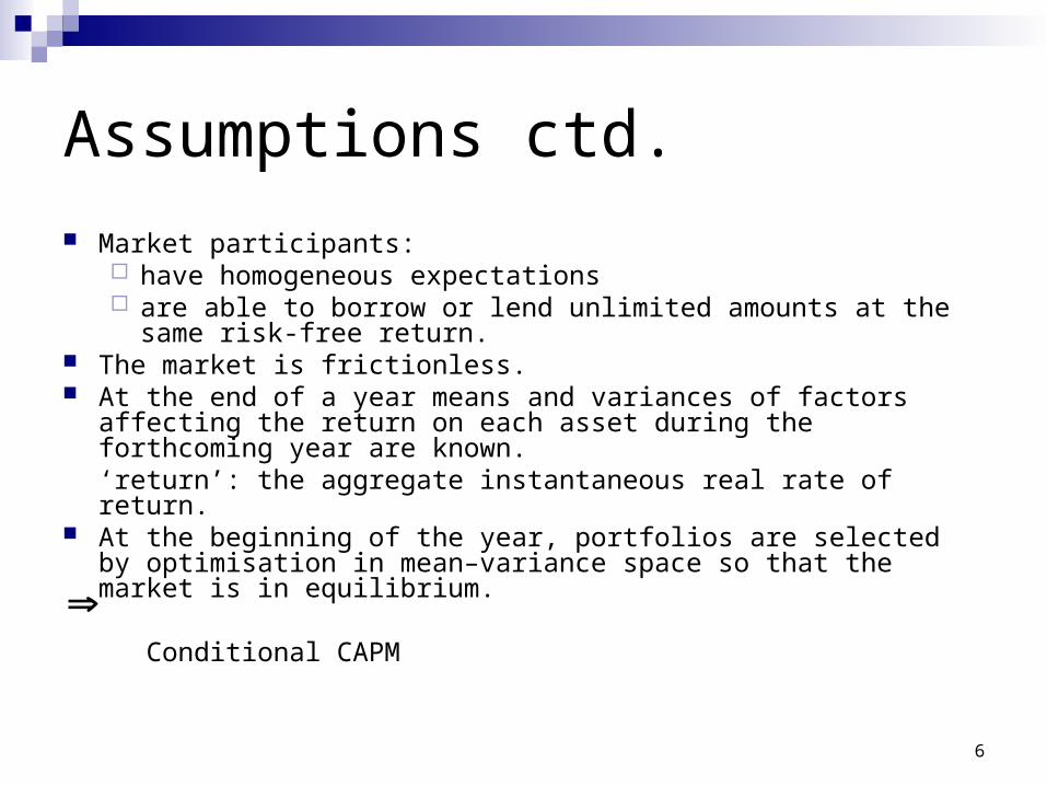
Assumptions ctd.

Market participants: have homogeneous expectations are able to borrow or lend unlimited amounts at the same risk-free

return. The market is frictionless. At the end of a year means and variances of factors affecting the return

on each asset during the forthcoming year are known.‘return’: the aggregate instantaneous real rate of return.

At the beginning of the year, portfolios are selected by optimisation in mean–variance space so that the market is in equilibrium.

Conditional CAPM

7

Agenda

Introduction Assumptions Prices and returns Notional risky assets Development of the model Summary of the model Parameter estimation Illustrative results

8

Prices & returns

Index-linked (zero-coupon) bonds (Real) risk-free rate Conventional (zero-coupon) bonds Inflation Equity

9

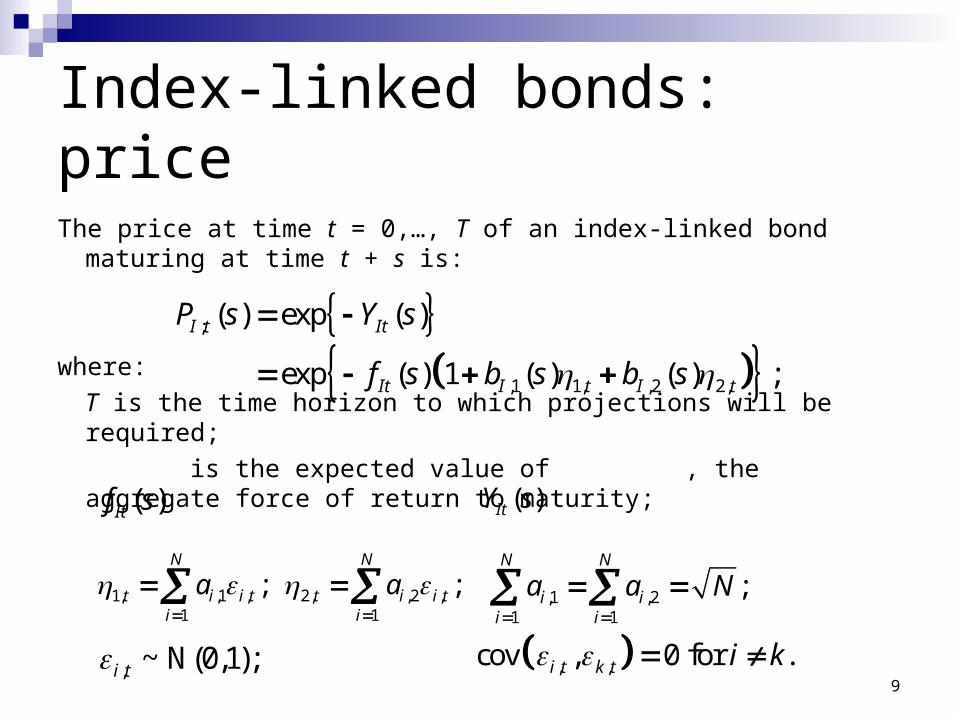
Index-linked bonds: price

The price at time t = 0,…, T of an index-linked bond maturing at time t + s is:

where:

T is the time horizon to which projections will be required;

is the expected value of , the aggregate force of return to maturity;

;

,1 1, ,2 2,

( ) exp ( )

exp ( ) 1 ( ) ( ) ;

I t It

It I t I t

P s Y s

f s b s b s

, ~ N(0,1);i t , ,cov , 0 for .i t k t i k

1, ,1 , 2, ,2 ,1 1

; ;N N

t i i t t i i ti i

a a

,1 ,21 1

;N N

i ii i

a a N

( )Itf s ( )ItY s

10

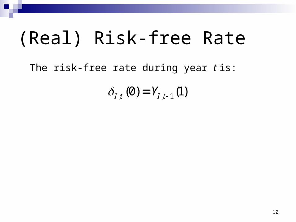
(Real) Risk-free Rate

; , 1(0) (1)I t I tY

The risk-free rate during year t is:

11

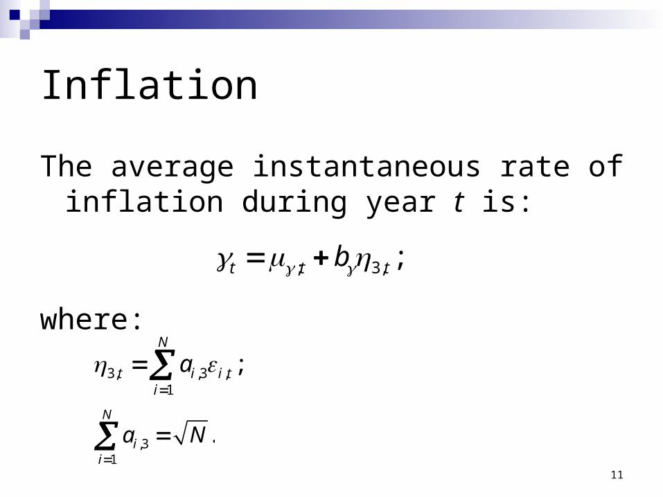
Inflation

The average instantaneous rate of inflation during year t is:

where:

; 3, ;t t tb

3, ,3 ,1

;N

t i i ti

a

,31

.N

ii

a N

12

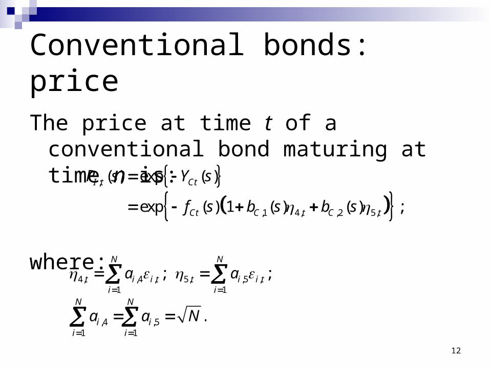
Conventional bonds: price

The price at time t of a conventional bond maturing at time n is:

where:

4, ,4 , 5, ,5 ,1 1

; ;N N

t i i t t i i ti i

a a

,4 ,51 1

.N N

i ii i

a a N

;

,1 4, ,2 5,

( ) exp ( )

exp ( ) 1 ( ) ( ) ;

I t Ct

Ct C t C t

P s Y s

f s b s b s

13

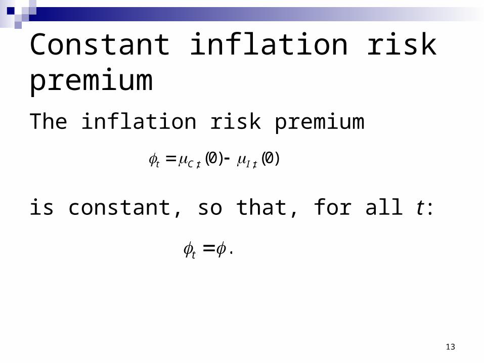
Constant inflation risk premium

The inflation risk premium

is constant, so that, for all t:

.t

; ;(0) (0)t C t I t

14

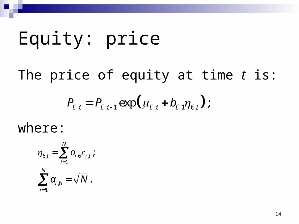
Equity: price

The price of equity at time t is:

where:

; ; 1 ; ,1 6,exp ;E t E t E t E tP P b

6, ,6 ,1

;N

t i i ti

a

,61

.N

ii

a N

15

Agenda

Introduction Assumptions Prices and returns Notional risky assets Development of the model Summary of the model Parameter estimation Illustrative results

16

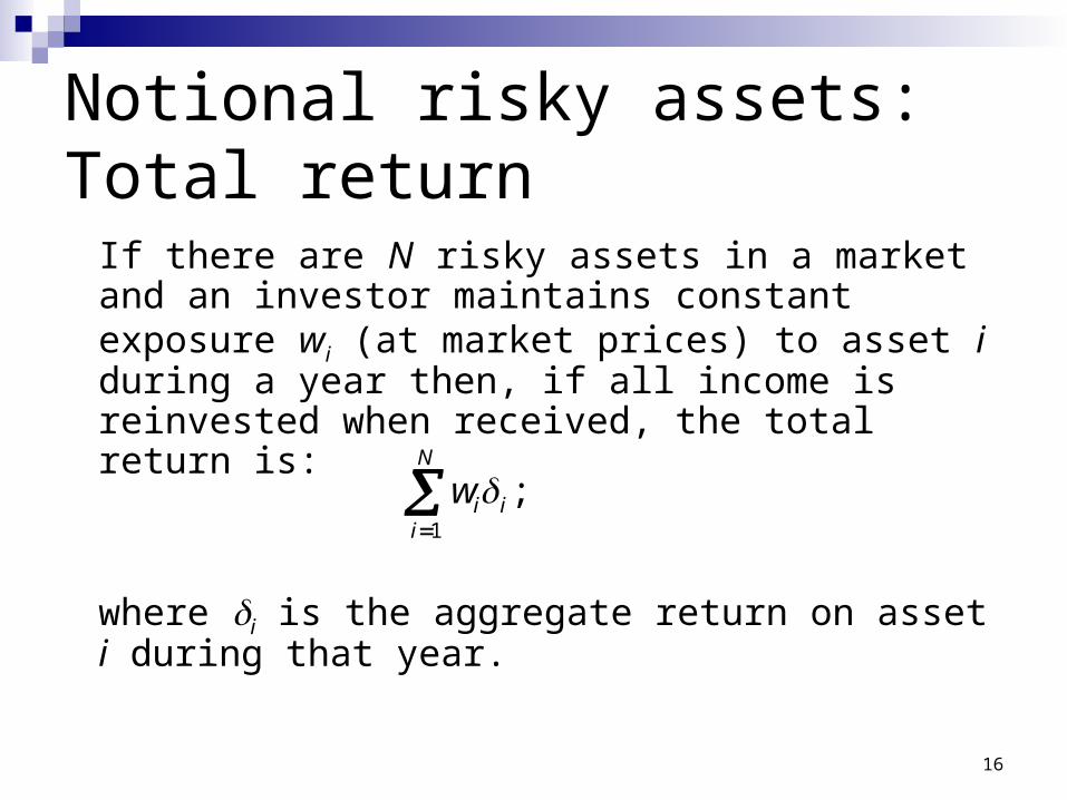
Notional risky assets: Total return

If there are N risky assets in a market and an investor maintains constant exposure wi (at market prices) to asset i during a year then, if all income is reinvested when received, the total return is:

where i is the aggregate return on asset i during that year.

1

;N

i ii

w

17

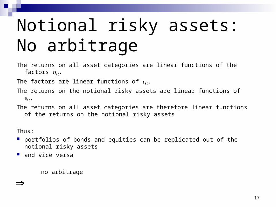
Notional risky assets: No arbitrage

The returns on all asset categories are linear functions of the factors j,t.

The factors are linear functions of i,t.

The returns on the notional risky assets are linear functions of i,t.

The returns on all asset categories are therefore linear functions of the returns on the notional risky assets

Thus: portfolios of bonds and equities can be replicated out of the notional risky assets and vice versa

no arbitrage

18

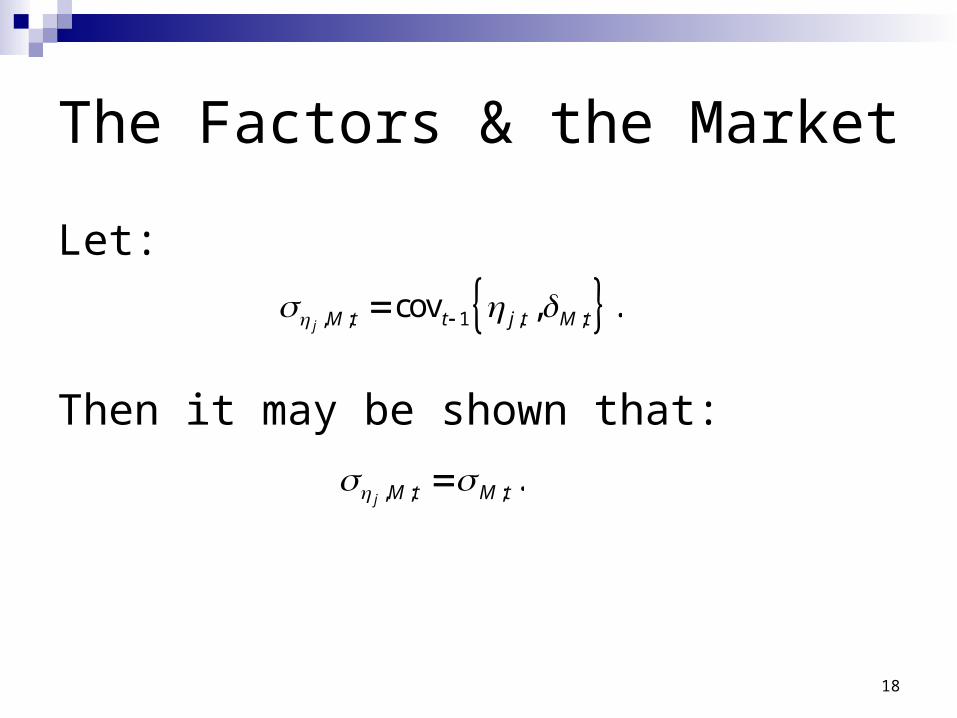
The Factors & the Market

Let:

Then it may be shown that:

, ; 1 , ;cov , .j M t t j t M t

, ; ; .j M t M t

19

Agenda

Introduction Assumptions Prices and returns Notional risky assets Development of the model Summary of the model Parameter estimation Illustrative results

20

Development of the model

The market price of covariance Index-linked bonds Conventional bonds Equity

21

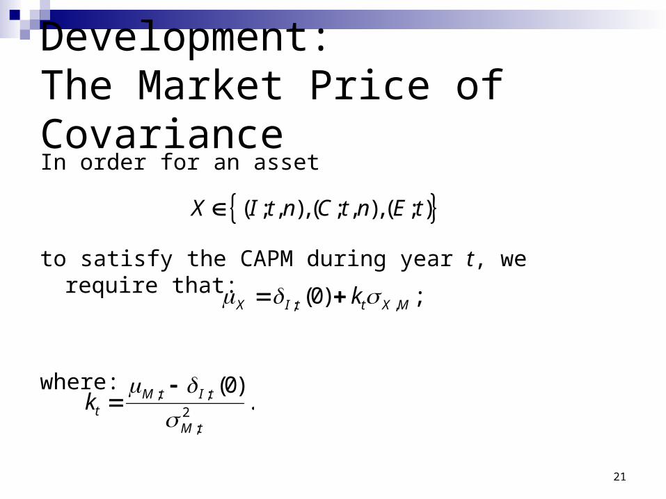
Development:The Market Price of CovarianceIn order for an asset

to satisfy the CAPM during year t, we require that:

where:

( ; , ), ( ; , ), ( ; )X I t n C t n E t

; ,(0) ;X I t t X Mk

; ;

2;

(0).M t I t

tM t

k

22

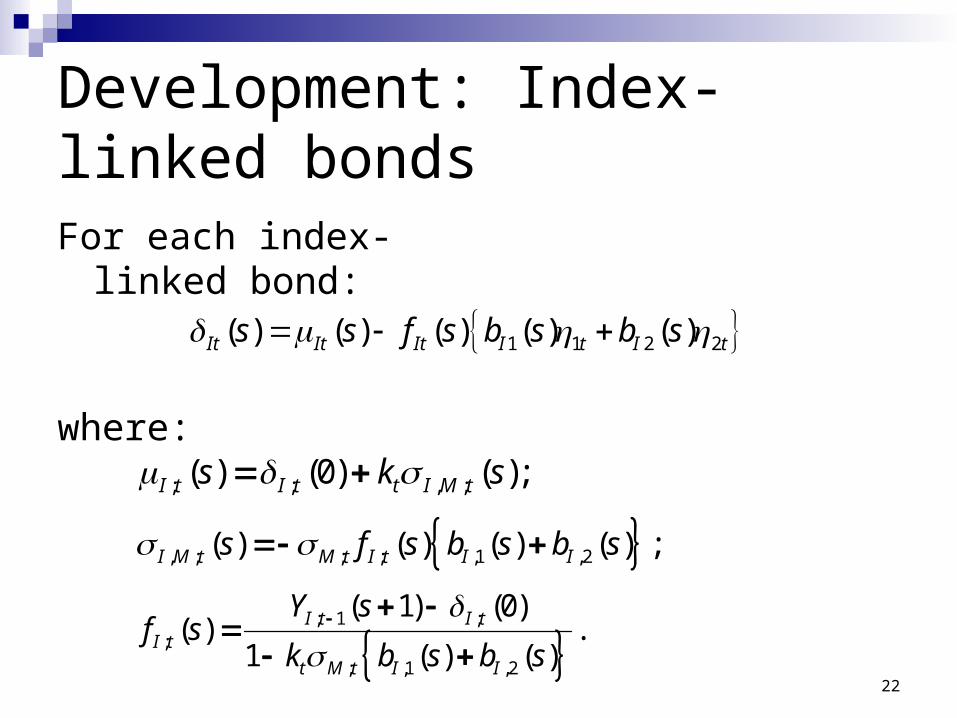
Development: Index-linked bonds

For each index-linked bond:

where:

; ; , ;( ) (0) ( );I t I t t I M ts k s

, ; ; ; ,1 ,2( ) ( ) ( ) ( ) ;I M t M t I t I Is f s b s b s

; 1 ;

;

; ,1 ,2

( 1) (0)( ) .

1 ( ) ( )I t I t

I t

t M t I I

Y sf s

k b s b s

1 1 2 2( ) ( ) ( ) ( ) ( )It It It I t I ts s f s b s b s

23

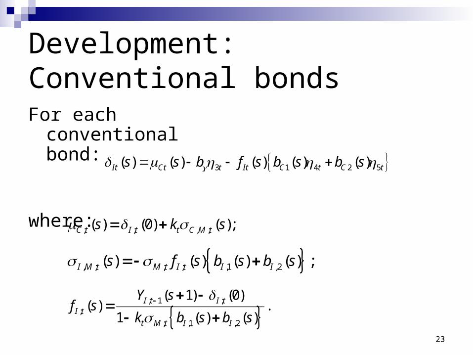
Development: Conventional bonds

For each conventional bond:

where:

; ; , ;( ) (0) ( );C t I t t C M ts k s

, ; ; ; ,1 ,2( ) ( ) ( ) ( ) ;I M t M t I t I Is f s b s b s

; 1 ;

;

; ,1 ,2

( 1) (0)( ) .

1 ( ) ( )I t I t

I t

t M t I I

Y sf s

k b s b s

3 1 4 2 5( ) ( ) ( ) ( ) ( )It Ct t It C t C ts s b f s b s b s

24

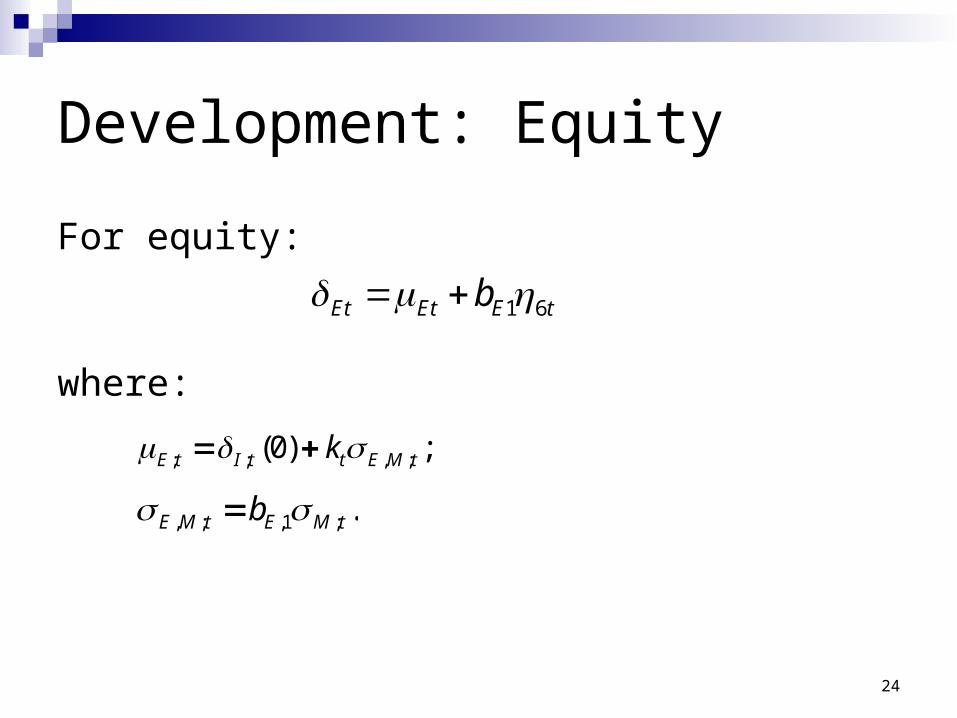
Development: Equity

For equity:

where:

; ; , ;(0) ;E t I t t E M tk

, ; ,1 ; .E M t E M tb

1 6Et Et E tb

25

Agenda

Introduction Assumptions Prices and returns Notional risky assets Development of the model Summary of the model Parameter estimation Illustrative results

26

Summary of the model

Parameters Variables

27

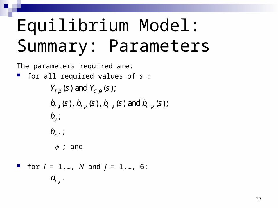
Equilibrium Model: Summary: ParametersThe parameters required are: for all required values of s :

; and

for i = 1,…, N and j = 1,…, 6:

,0 ,0( ) and ( );I CY s Y s

,1 ,2 ,1 ,2( ), ( ), ( ) and ( ); I I C Cb s b s b s b s

;b

,1;Eb

, .i ja

28

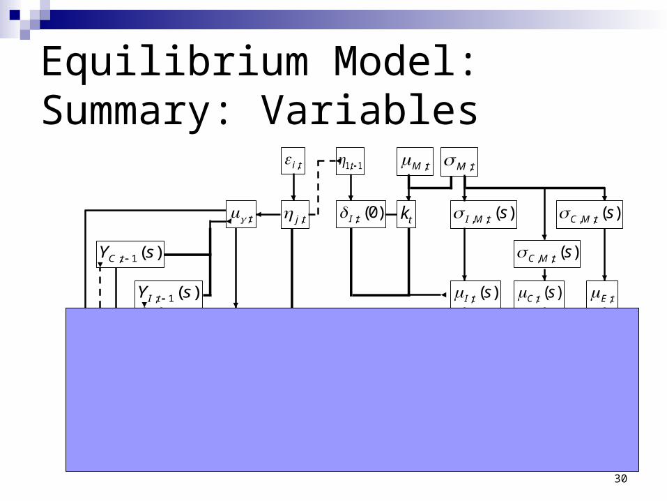
Equilibrium Model: Summary: Variables

1, 1t

; (0)I t

;M t ;M t

tk , ; ( )I M t s

, ; ( )C M t s

; ( )I t s ; ( )C t s ;E t

, ; ( )C M t s

29

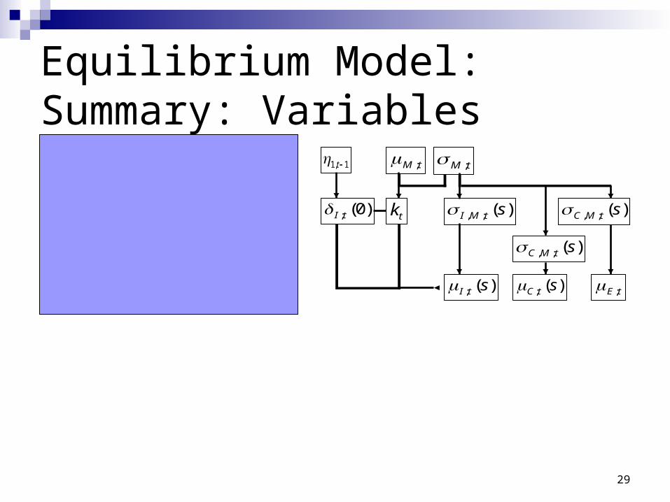
Equilibrium Model: Summary: Variables

,i t

;t ,j t

1, 1t

; (0)I t

;M t ;M t

tk , ; ( )I M t s

, ; ( )C M t s

; ( )I t s ; ( )C t s ;E t

, ; ( )C M t s

; 1( )C tY s

; 1( )I tY s

30

Equilibrium Model: Summary: Variables

,i t

;t ,j t

1, 1t

; (0)I t

;M t ;M t

tk , ; ( )I M t s

, ; ( )C M t s

; ( )I t s ; ( )C t s ;E t

;E t; ( )I t s ; ( )C t s

; ( )I tY s

, ; ( )C M t s

; 1( )C tY s

; 1( )I tY s

; ( )C tY s

;t

31

Summary of the model

The equilibrium model: allows for any type of model of the market portfolio models bonds, ‘equity’ and inflation maintains equilibrium each year is arbitrage-free is linear uses discrete time but allows for intra-year variability assumes mean–variance decision-making uses a conditional CAPM focuses on a local market

32

Agenda

Introduction Assumptions Prices and returns Notional risky assets Development of the model Summary of the model Parameter estimation Illustrative results

33

Parameter estimation:Variables used for various asset classes Equity: FTSE All-Share TRI Conventional and Index-Linked Bonds: UK

DMO zero-coupon curves Inflation: UK retail prices index

34

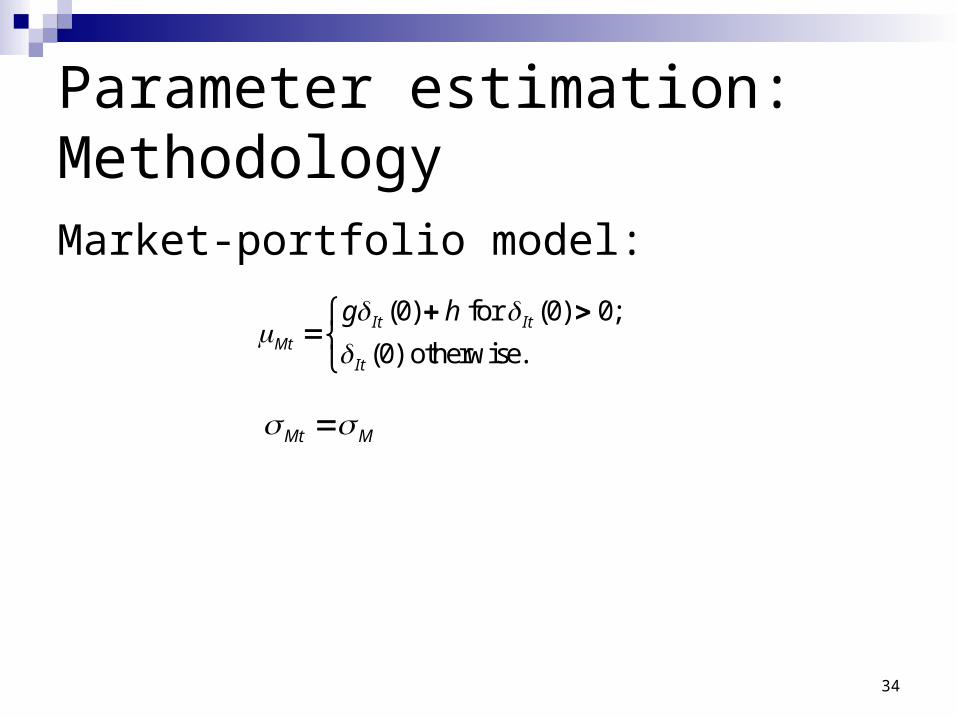
Parameter estimation:MethodologyMarket-portfolio model:

(0) for (0) 0;

(0) otherwise.It It

MtIt

g h

Mt M

35

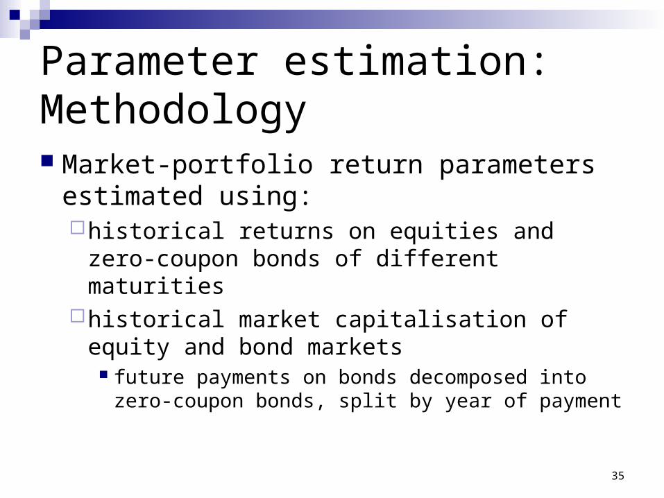
Parameter estimation:Methodology Market-portfolio return parameters estimated

using:historical returns on equities and zero-coupon

bonds of different maturitieshistorical market capitalisation of equity and bond

markets future payments on bonds decomposed into zero-

coupon bonds, split by year of payment

36

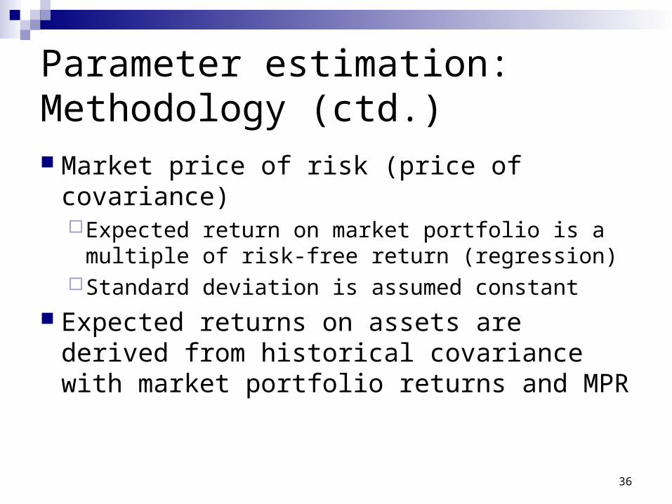
Parameter estimation:Methodology (ctd.) Market price of risk (price of covariance)

Expected return on market portfolio is a multiple of risk-free return (regression)

Standard deviation is assumed constant

Expected returns on assets are derived from historical covariance with market portfolio returns and MPR

37

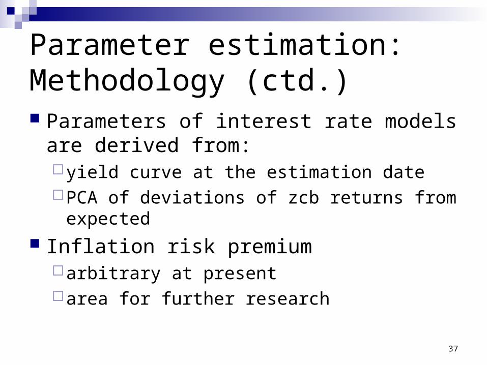
Parameter estimation:Methodology (ctd.) Parameters of interest rate models are derived

from:yield curve at the estimation datePCA of deviations of zcb returns from expected

Inflation risk premiumarbitrary at presentarea for further research

38

Agenda

Introduction Assumptions Prices and returns Notional risky assets Development of the model Summary of the model Parameter estimation Illustrative results

39

Illustrative results

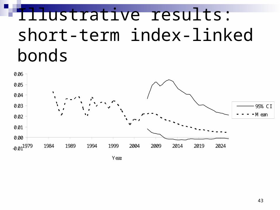
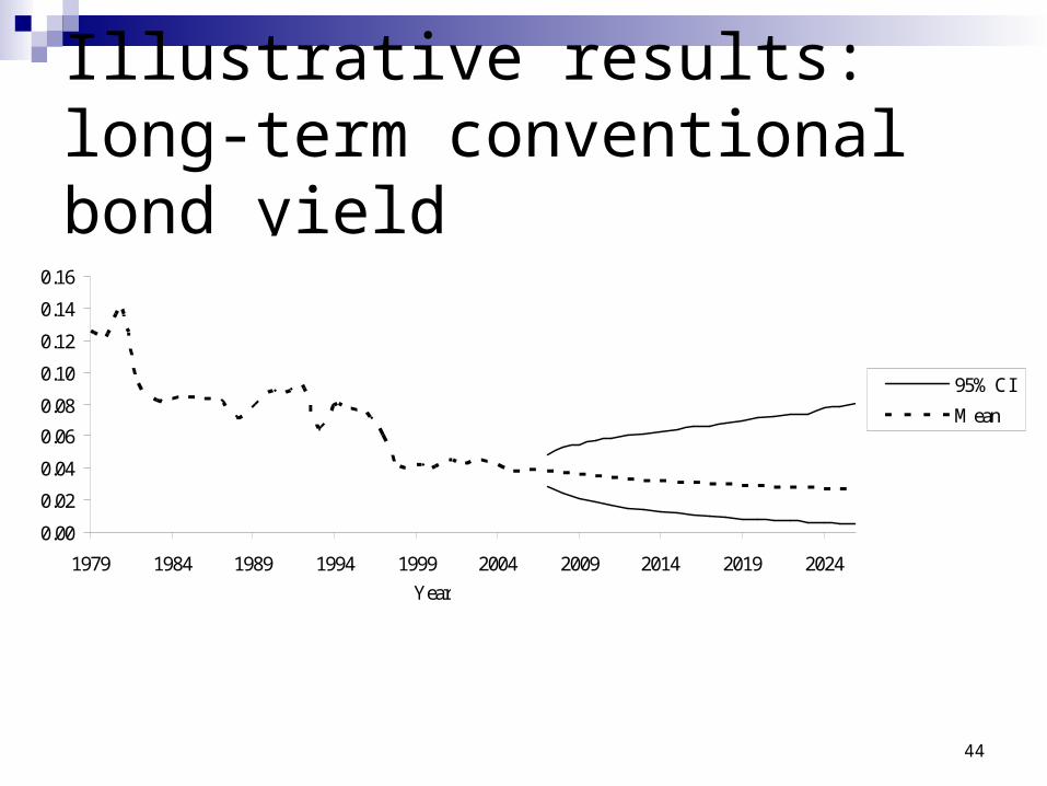
10 000 simulations for each economic variable 20-year projection mean and 95% CI

40

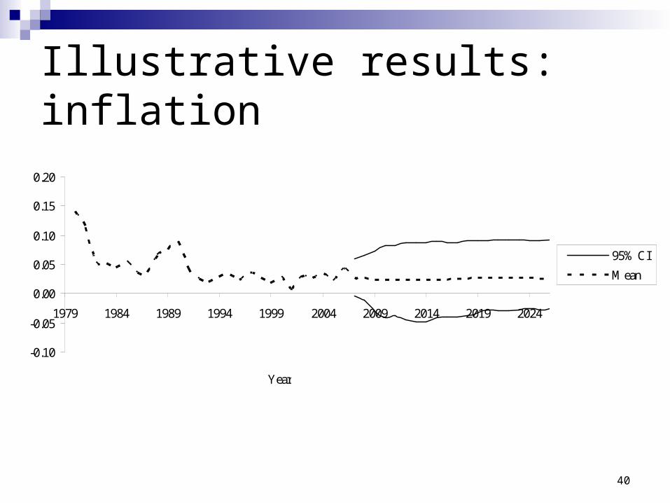
Illustrative results: inflation

-0.10

-0.05

0.00

0.05

0.10

0.15

0.20

1979 1984 1989 1994 1999 2004 2009 2014 2019 2024

Year

95% CI

Mean

41

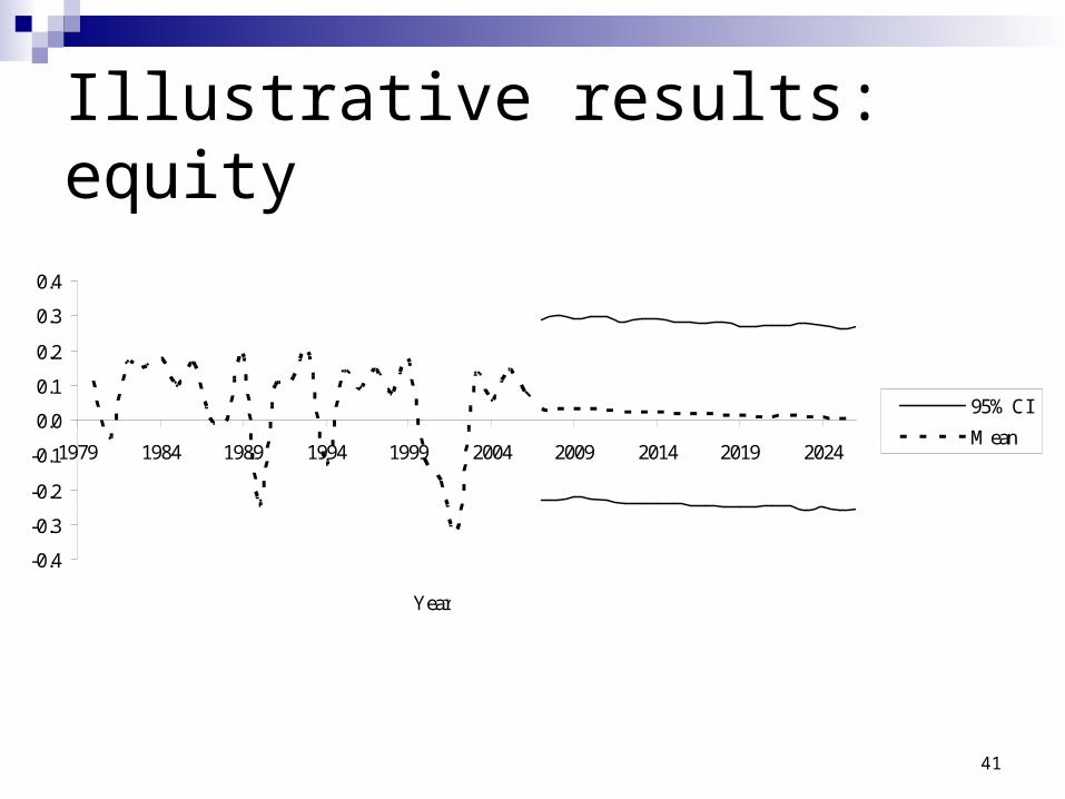
Illustrative results: equity

-0.4

-0.3

-0.2

-0.1

0.0

0.1

0.2

0.3

0.4

1979 1984 1989 1994 1999 2004 2009 2014 2019 2024

Year

95% CI

Mean

42

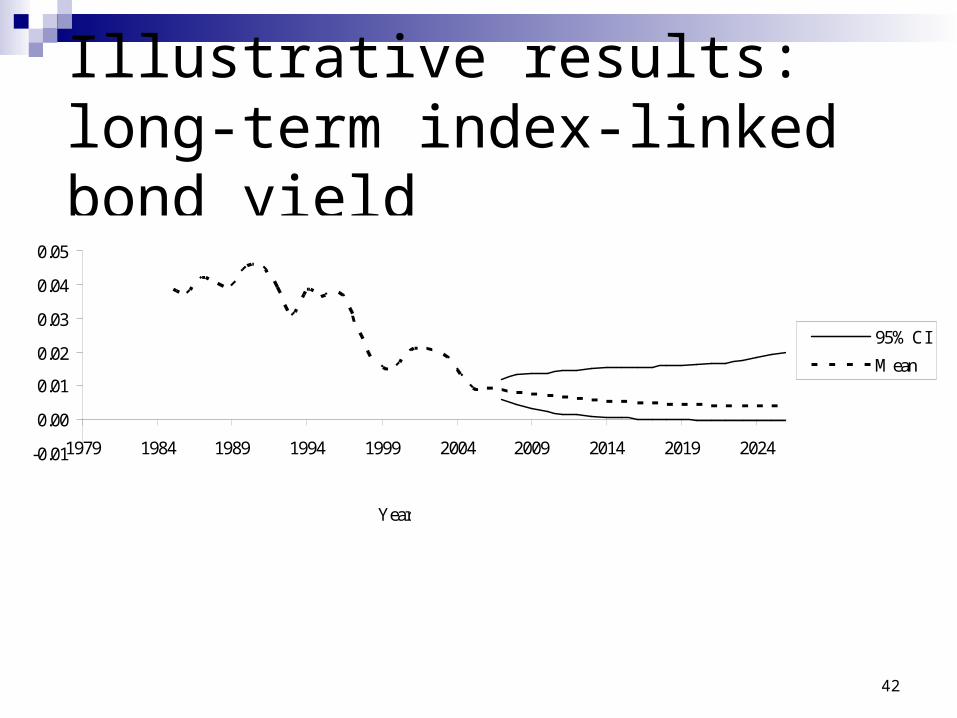
Illustrative results: long-term index-linked bond yield

-0.01

0.00

0.01

0.02

0.03

0.04

0.05

1979 1984 1989 1994 1999 2004 2009 2014 2019 2024

Year

95% CI

Mean

43

Illustrative results: short-term index-linked bonds

-0.01

0.00

0.01

0.02

0.03

0.04

0.05

0.06

1979 1984 1989 1994 1999 2004 2009 2014 2019 2024

Year

95% CI

Mean

44

Illustrative results: long-term conventional bond yield

0.00

0.02

0.04

0.06

0.08

0.10

0.12

0.14

0.16

1979 1984 1989 1994 1999 2004 2009 2014 2019 2024

Year

95% CI

Mean

45

Illustrative results: short-term conventional bond yield

0.00

0.02

0.04

0.06

0.08

0.10

0.12

0.14

0.16

1979 1984 1989 1994 1999 2004 2009 2014 2019 2024

Year

95% CI

Mean

46

Conclusion

The equilibrium model: allows for any type of model of the market portfolio models bonds, ‘equity’ and inflation maintains equilibrium each year is arbitrage-free is linear uses discrete time but allows for intra-year variability assumes mean–variance decision-making uses a conditional CAPM focuses on a local market