IEEE Transactions on Power Apparatus and Systems, vol . PAS-94, no. 2 , March/April 1975

J. F. Dopazo

S T O C H A S T I C L O A D FLOWS

0. A. Klitin

American Electric Power Service Cow. N. Y., N. Y.

A. M. Sasson

Abstraci:

The load flow study has been at the center of studies made for designing and operating power systems for many years. I t i s well known that forecasted data used in load flow studies contain errors that affect the solution, as can be evidenced by running many cases perturbing the input data.

This paper presents a method for calculating the effect of the propagation of data inaccuracies through the load flow calculations, thus obtaining a range of values for each output quantity that, to a high degree of probability, encloses the operating conditions of the system.

The method is ef f ic ient and can be added to any existing load flow program. Results of cases run on the AEP system are included.

Introduction

The load flow study has been at the center of analysis made to design power systems and delineate operating practices. From the studies performed in network analyzer days to the sophisticated digital computer programs of today, conceptually speaking, not much alteration has taken place to the definition of the load flow problem, The fast methods availablenow, with their efficient uti- lization of computer core and their capability of access to large data fi les, have made possible for the engineer to run a largenumber of cases, starting from some base system condition, to study his design or his proposed plan of operation under many alternatives. Important decisions evolve from these studies.

For each load flow case that i s solved, it i s necessary for the engineer to provide the required data that define the conditions for the case, This data usually include real and reactive loadings at so-called load busses and real power generation and voltage mag nitude at generator busses, as well as the electrical characteristics of the system model.

The formulation of the load flow problem assumes that the data providedisabsolutelypreciseand providesresults totally compatible with the given data apart from round-off errors. However, in practice, it can be readily appreciated that load flow data can only be known within some finite precision, this being more the case as the study represents conditions that are more distant into the future. As a normal screening process, the engineerlooks at the range of possible values for a particular piece of data and setects an average value as the number to be used in the load flow study.

Given the importance of the decisions that evolve from load flow studies, i t appears that it i s important to know the possible

ranges of result quantities corresponding to the known range of data quantities. In other words, it i s of interest to determine the effect on load flow results of our ignorance of input data values.

This paper w i l l address i tsel f to the problem of processing the expected errors in the data of the load flow problem, assuming that the electrical characteristics of the model are known sufficiently well that the effect of their inaccuracies i s negligible.

Essentially, the method converts the load flow problem formu- lation from a deterministic one to a stochastic one. The results obtained can be considered to define the range of variation of result quantities, thus determining the worst conditions for each. Similar results to those obtained with the stochastic load flow can be arrived at by repeating a large number of conventional deterministic load flow cases in which for each case the data i s perturbed, such that thevarious cases represent possible sets of data within the precision that the data i s known. Once a l l these studies have been carried out, the range of values for a specified result quantity can be identified. What the stochastic load flow does i s to obtain these ranges in one direct calculation. An important practical characteristic of the method i s that it can be added to any existing load flow program since the process requires f i rst the solution of a conventional load flow, followed then by a series of steps that determines the prop- agation ofthe errors of input data. The method i s not only applicable to the load flow problem but to any problem where the model i s a system of a sufficient number of equations.

MATHEMATICAL BACKGROUND

The method i s based on the principles of statistical least squares estimation for linear systems. Some of the in i t ia l ideas of the stochastic load flow came about from the experience obtained with simulation of and testing on the AEP monitoring project [ 1-61. The derivation of some of the equations to be presented can be found in these references or in advanced statistical texts.

Given a non-linear set of equations,

y ' = f ( x ' ) + E

a Taylor's series expansion can be used to linearize (l),

y = J x + E

where y = y ' - f ( x ) I o x = x ' - x b J = Jacobian o f f ( x f ) E = vector of error random variables

Equation (1) i s interpreted in thefollowing way. There are data quantities y which represent the average value o f the range of possible values the piece of data may have according to some statistical distribution defined from our physical knowledge of the problem and the methods that were used to forecast the data. There are problem variables x ' from which all quantities can be

Paper T 74 308-3, reco-nded and approved by the IEEE Power System computed. These variables have a true, although unknown, value at the Summer Resources Conf,, Anaheim, which represent conditions as they wi l l exist at some future date. JUIY 14-19, 1974. Manuscript submitted n gust 29, 1973; made available for The Vector E represents the error between y ' and f As Engineering Committee of the BEE Power Engineering Society for presentation

printing April 3,1974. wil l not be known until the future conditions are encountered, E can

299

only be described statistically as a random variable that has some deviation of G from Xt. Equation (13) presents the variance of $3) mean and variance that represent our expectations of the way E and Equation (14) says that this variance i s zero ifJhere are as could vary. The meanings of y and X are similar to those of y ' and many equations as unknows. Th is simply means that y i s equal to

The following will assume the linearization presented in Equa- y, or that the actual solution of Equation (2) has tieen obtained, a tion 2. fact also reflected in that F(3 = 0.

The statistics of the vector E can thus be specified as Another statistical property i s that

E (€ ) = O E ( E E ~ ) = V

F(x) = (y-Jx)tV-l (y-Jx) (4) Assuming that there are other quantities z ' related to x ' as

and the value of x that minimizes F(x) is cal led 4 and i s given by follows, [61

Z ' = g ( x ' ) ( 17) 4 = ( J k l J ) - l J N - l Y

(5) a Taylor's series expansion of g linearizes (17) into which reduces to

z = K x (18) 2 = J - l y (6) from which ?can be obtained from 2,

for the case that J i s a square matrix, implying the same number of A

equations as unknowns. F(Q) i s equal to zero for th is case. z = K 2 (19)

As the original Equation (1) was nonlinear, 12 should be inter- preted as the converged value after some iterations in which J i s recomputed in each iteration. Z t = K x t

and z-tfrom X t

Corresponding to $there i s a 3 computed directly from Equation The statistical properties of z can be summirized as follows:

E(?) = Z t (21) 9 = J ; (7)

and corresponding to the true, but unknown value of X, called X t

there i s a true, and also unknown, value of y, called yt, Equation (22) presents the variance of 2 Yt = J X t (*) Statistical Properties: Confidence Limits

(a,

E ( ( k t ) (z*-zt)b = K ( J ~ v - ~ J ) - 1 ~ t (22)

Statistical Properties: Expected Values nd Variances It i s now necessary to mention the probability distribution characteristics of the various quantities. The input quantity y can

The quantities 2, X , Y, F and Yt have known Statistical Prop have m y probability distribution function, which is known from the erties that are of interesf, knowledge of the physical problem at hand. Its statistical properties

given in Equation (3) can then be computed. The output quantities E($) = x t (9) x or z are linear combinations of y and by the Central L imi t Theorem

can be taken as norm2lly distributed random variables. It can then E {(x^-xt) (c-t)t } = (J tV-1J) -1 (10) be said that and z are N(q, ~ ~ 2 ) and N(zt, oZq respectively.

(11) A normally distributed random variable can always be trans- formed into a unit normal, thus

which reduces to the following if J i s a square matrix, A z - Z t (24) - = N(0, 1)

EUEY) (?-v)t> = 0 (14)

Equations (9) and (11) imply that if E h 3 the statistical prop- erties given in Equation (31, then, i f 3 and y had been detymined ox2 = diag {(JW-lJ)- l } (25) many times from different values of y, the average of :and y tends to the true values of x and y. In statistical terms this is called an uz2 = diag {K(JtV-lJ)-lKt) (26) unbiased process.

Although Xt and z tare not known, a statement can be made as Equation (10) presents the variance of :which represents, the to a range which encloses them with some probability of being

U Z

where

300

correct. Within a range of. f 3 times the unit standard deviation of the random variables defined by (23) and (24), it can be said that there i s approximately a 99%probability ofenclosing thetrue values.

Thus, it can be stated that

X t = x ^ * 3 ux (27)

Z t = z f 3 U Z (28) A

with a 99% probability of being correct.

THE LOAD FLOW PROBLEM

The previous section presented the general theory required for the stochastic load flow. This section will relate that theory to the load flow problem. The various quantities referred to in the previous section w i l l now be defined in terms of the variables familiar to the load flow.

refers to load flow data, that is, load bus P and Q and generator bus P and E.

refers to bus state variables E and s

refers to me variances of the errors assumed on the y input data.

refers to the Jacobian of the load flow equation, that i s the partials of P, Q and E input quantities y with respect to E and s load flow variables X.

refers to output quantities of the load flow computed from X ,

such as, line flow P and Q and generator bus Q.

refers to the Jacobian of output quantities z with respect to load flow variables X.

torization techniques can then be used to triangularize this matrix and repeated back substitutions wi l l y ie ld the elements of the covariance matrix. It i s only necessary to save those terms that structurally are in the same positions as the original JtV-lJ and then only a symmetrical part. Th is is an important characteristic since, in general, the Cov (x) is a fu l l matrix.

Step 3 - Computation of Covariance Matrix of 2 The covariance matrix of ;was given in Equation (22) as

COY($ = K ( J ~ v - ~ J ) - ~ K ~ (22)

To calculate the Cov(?) the Jacobian of output quantities z must be calculated. The structure of this matrix i s also dependent on that of the admittance matrix and is thus related to that of J. Matrix K i s thus a sparse matrix and should be calculated as such. Because of i ts structural relationship to J, in the triple product^ indica ed in Equation (22) only JtV-lJ structured elements of ( J V - t J ) - l are needed. This is the reason for saving only those elements in Step 2. In the case of Equation (22), only diagonal elements need be computed and saved. Step 4 - Computation of Confidence Limits

and (28) as Confidence Limits for 2 and ? were given in Equations (27)

X t =;" + 3 u x

z t = z * 3UZ A

The u z vector are the diagonals of the Cov(9 while the C$ vector are l h e diagonals of the Cov(?). Those elements of these two matrices have been already calculated and saved in Steps 2 and 3.

AREA CONSTRAINTS Having related the variables used in the Previous Section to

those of the load flow problem, they shall be used interchangeably The stochastic load flow, as presented in the previous section, in what follows. The various steps of the process wi l l now be amounts to summarizing the results of many load flows, as far as presented. the quantities obtained in the confidence l imi ts are concerned.

These load flows could have beenrun perturbing all input quantities according to the statistics of the uncertainty of these values as derived from the knowledge of the physical problem. The results

The first step i s to compute as 'Iwwn in generation decreased, forcing the slack generator to have wide would reflect cases in which total load was increased with maybe

(6) with an iterative process to take into account the non-linear limits. This situation might be imp,.,.,ved if there is additional nature of the load flow equations, Equation (1). Equation (6) shows information available. In addition to the forecast made on individual that for the Of number Of equations as unknowns' the loads and generators, i t i s often the case that total load and gener- statistical properties of the errors of Y drop out of the equations. ation of given areas of the system are known to a greater precision. This converts Equation 6) to imply the solution Of a load flow I f conventional load flows were run perturbing the data, area load data quantities y. Any existing load flow program can be used in problem with average IWnerical values ass i f led to the load flow and generation constraints would be used to restrict the data.

this f irst step, thus making this step equivalent to the solution of Area load and generation constraints can be included in the the problem as i s done in Practice, with average values for the stochastic load flow. An area constraint acts as an additional forecasted input data. equation in Equations (1) and (2). The additional equation i s ob

Step 2 - Computation of Covariance Matrix of 2 tained by adding some of the other equations already included in (1) and (2).

The covariance matrix of x" was presented in Equation (10) as For example, i f the loads of nodes 3, 5 and 7 are to be con- strained to a finer degree, new equations are formed,

St@ 1 - A Load Flow

C O V ( ~ = ( J ~ v - ~ J ) -1 (10) P n t l = P 3 + P 5 + 4 + c p , n t l (29)

To calculate the Cov(;), the Jacobian of the load flow equation must be f i rst formed and evaluated at the solution point of the Qn+ 1 = Q3 + Q 5 + Q 7 +Eq,n t 1 load flow of Step 1. Sparsity techniques should be used as both J and JtV- lJ a e s arse matrices. An ordering scheme should be This new equation appears asthe equation of a new imaginary node, used to order J \ ! V - J. In the same way that the structure of the connected to 3,5 and 7 and to al l nodes to which these are connect- admittance matrix Y can be used to order J in a ewton's load flow, ed to. However, the new node does not contribute any new variable the structure of YtY can be used to order JtV- Y J. Triangular fac- x to the problem, thus making J a non-square matrix. It i s important

301

to realize that even i f J i s non-square i n Steps 2, 3 and 4, this does 1. Area constraints deteriorate the sparsity of the state in- not alter the fact that a conventional load flow Program can be verse covariance matrix as their effect is similarto the introduction used in Step 1. This comes from the condition that the solution Of of a node connected to a l l other nodes in the area. In the limit, the original n equations i n (2) auhmatically solve the additional considering the entire system as one single area, this matrix be- equations introduced by the area constraints. comes full.

The inclusion of area constraints as presented in Eq. (29) con- siders the input covariance matrix to be diagonal making the addi- tional equations independent from the original set. Considering an area of k nodes, Eqs. (1) become

Yi = 4 i Iy) + Ei, i = I, ... k (30)

which Eq. (29) has the form

The relation between Eqs. (30) and (31) i s the following, k k

f n t I (X) = 5 +i (x) = f (Y’i - c i ) I

(32) Substituting in Eq. (31),

(33)

2. Confidence limit results would, in general, be somewhat sensitive to slack bus location.

The above limitations can be easily overcome by modelling the load flow slack bus as any other generator bus, with P and E equations but allowing only E to be a state variable, keeping 6 fixed. The forecasted error in total system load plus losses can be distributed among generator Pequations, thus making a l l generators CDmpensate for forecasting errors. It is not necessary to divide the total expected error evenly among generators. No area constraints are used,

The changing of position for the angle reference bus has no effect on confidence limits other than those of voltage angles them- selves. As angles are really angle differences between busses and the reference bus, these values and their confidence limits are dependent on the reference bus location. However, the confidence limits of angular differences between any two busses are inde- pendent of reference bus location.

(34’1

It is of interest to compare Eqs. (31) and (34). The area constraint formulation considers

However, had y’n t 1 been defined as in Eq. (34), the statistics of E’n t 1 would have been the following, assuming independence,

E ( € ’ , t I E ’ n t l ! Vi t V n t I (38)

Eqs. (37) and (38) show that there i s a distinct difference between modelling the area constraint as afunctionofastationary true value

k

I

and as the sum of random variables.

CONSTRAINT ON TOTAL SYSTEM LOAD

The previous sections have shown that the stochastic load flow represents the combined results of many deterministic load flows. Two types of load flow runs have been modelled:

1. Asetof load f lows in which each piece of data i s randomly varied. It was discussed that this should produce large confidence limits for the slack generation and for lines near that bus due to some cases representing changes in total load and in generator outputs.

As in the case of area constraints, the reference bus equation is considered to be an independent equation. The modelling of the reference bus equation is made as a function of the system state variables and not by adding a l l other inputs. This model also reflects the nature of the distribution of uncertainties through- out the system to be one of non-simultaneity of occurrence of indi- vidual uncertainties and not one of correlation.

Of negligible effect is the condition of having one extra equa- tion, producing an overdetermined set of input equations and a filtering effect.

SOLUTION OF PRACTICAL CASES

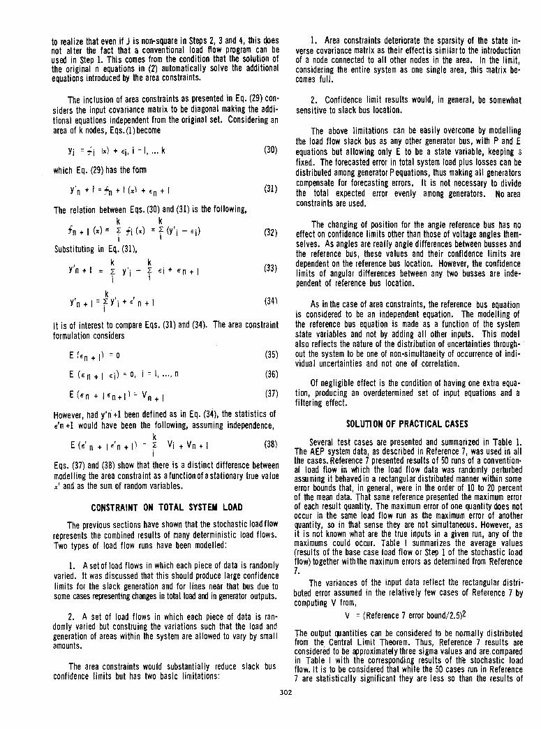
Several test cases are presented and summarized in Table 1. The AEP system data, as described in Reference 7, was used in a l l the cases. Reference 7 presented results of 50 runs of a convention- al load flow in which the load flow data was randomly perturbed assuming it behavedin a rectangular distributed manner within some error bounds that, in general, were in the order of 10 to 20 percent of the mean data. That same reference presented the maximum error of each result quantity. The maximum error of one quantity does not occur in the same load flow run as the maximum error of another quantity, so i n that sense they are not simultaneous. However, as it i s not known what are the true inputs in a given run, any of the maximums could occur. Table I summarizes the average values (results of the base case load flow or Step 1 of the stochastic load flow) together with the maximum errors as determined from Reference 7.

The variances of the input data reflect the rectangular distri- buted error assumed in the relatively few cases of Reference 7 by computing V from,

2. A set of load flows in which each piece of data is ran- V = (Reference 7 error bound/2.5)2 domly varied but construing the variations such that the load and

amounts. from the Central Limit Theorem. Thus, Reference 7 results are considered to be approximately three sigma values and are compared

The area constraints would reduce slack bus flow, It i s to be considered that while the 50 cases run in Reference in Table I with the corresponding results of the stochastic load

confidence limits but has two basic limitations: 7 are statistically significant they are less so than the results of

generation of areas within the system are allowed to vary by small The oubut Wantities Can be considered to be normally distributed

302

say 100 or 500 cases. In essence, the stochastic load flow sum marizes the results of a greater number of cases than the 50 of Reference 7.

Table I presents results of some typical output quantities. In particular, i t i s of interest to look at the flows in lines near the slack bus, bus number 1. These are presented in the f i rst 8 rows in Table I. The next two groups of 3 rows each refer to l ines in two different sections of the system, both removed from the slack bus. The following group of 3 rows refer to generation results at the slack bus and two other generators. Since the real powers of the last two generators are data quantities they are not included in Table I. The last group of 3 rows presents the wltage magnitude and angle at three different busses, bus 21 being a generator bus.

The six cases presented in Table I are now discussed:

Case 1

Case 1 i s referred to as the Fixed Voltages case in Table I. In this case generator bus voltage magnitudes were considered to be fixed, al l other quantities having the bounds given in Reference 7. A comparison with the results of Reference 7 shows that the real line flow Confidence Limits are of the same order of magnitude, actually slightly larger. Reactive flow for l ines near the slack bus are smaller in Case 1, the same being tnre for the results of r e active generation.

Case 2

Case 2 i s referred to as the Variable Voltages case in Table I. For this case generator voltage magnitudes were considered both as

TABLE 1 - STOCHASTIC LOAD FLOW TEST CASES

input quantities and as variables Of the stochastic load flow, A comparison with Case 1 shows that results are very similar except for reactive generation and reactive flow of llnes near the slack bus. An error bound of 1.2 percent was assumed at a l l generator busses, this being the only error bound data not being identical to that of Reference 7, although it i s of the same order of magnitude.

Cases 1 and 2 appear to draw the following two conclusions:

1. The linearization implied in going from Equation (I) to Equa- tion (2) is val id for the level of error bounds considered.

2. The decoupling of P-s and Q-E quantities in the load flow is visible in the comparison of the two cases. The addition of voltage magnitude variations had a considerable effect on re- active flow and generation, and a negligible one on real power flow and angles.

Case 3

Case 3 includes additional constraints, in both load and gen- eration areas, sllch that the total load or generation of each area has an error bound of 5% of the average total load or generation for the area. A l l other input quantities have individual bounds as in Case 2.

The results of Case 3 show a general attenuating effect on the Confidence Limits of all quantities, especially those near the slack bus. This is as expected. In reference 7, and in the equivalent results of Cases 1 and 2, the data used for the load flows implied situations where the total load was increased or decreased from the average value, the slack bus having to adjust the differences. As a

C O N F I D E N C E L I M I T S

FLOW BETWEEN BUS TO BUS 1 38 1 2 1 3

38 39 38 40 40 43

3 7 7 12

16 20 15

15 9

33 32 32 37 37 36 GENERATION

AT BUS

1 21 40

VOLTAGE AT BUS

10 21 39

AVERAGE VALUES

-118-J 68 515tJ 51 237-J 0 680 -J695

1 -J380 733 -J130

-1Ol tJ 39 -158tJ 8

- 96-J 63 -102-J150 -184tJ 51

-260-J 34 -222-J 15 229-J 28

634-J 17 - 3 5 t J 59 800 -J200

9 m 1 . o u

9 u

REFERENCE 7

411 tJ245 7 8 t J 9 1

162tJ 63 163tJ 51 272 +J 174 208 tJ163 175tJ 99 152 tJ163

8 1 t J 35 50 tJ 31 39 +J 33

42 t J 23 47tJ 19 53tJ 28

609 t J334 J377 J 540

0.8514.91

CASE 1 FIXED

VOLTAGES

130tJ 19 191tJ 4 218tJ 48 321tJ 14 250 tJ102 205tJ 25 219tJ 51

7 6 t J 50 5 5 t J 44 5 3 t J 42

6 2 t J 24 6OtJ 13 6 1 t J 22

505tJ 5

773 t J 21 J117 J105

3 . 6 0 u

0.3016.36 L m

CASE 2 VARIAELE

VOLTAGES

?!I! 191 t J 48 218 t J 56 32 1 t J 166 249 tJ201 206 +J 102 219 tJ138

76 tJ 51 56 +J 44 53 +J 43

62 +J 28 60 +J 19 61 +J 26

173 tJ200 J347 J5D6

3.8015.35 1 . 4 0 w . 9 O W

CASE a 5% AREA

CO"lNTS(1) 180 tJ148 6 2 t J 63 72 t J 40 97.tJ 32

131 t J 139 109 tJ148 94 t J 83

110 tJ113

40 t J 29 40 +J 36 34 +J 32

50+J 21 48 +J 14 49 +J 19

264 tJ166 J272 J413

1 . 7 0 u 1 . 2 o w 0.7012.48

CASE 4 CASE 5 2XAREA

CASE 6 5% AREA 3% TOTAL LOAD

CollsmlwTs COWSTRAINTS(2) c&srrWwT 9ftJ148 214tJ148 54 tJ206 5 t J 63 4 9 t J 62 55 t J 88 4 3 t J 40 7 6 t J 29 99tJ138 94 +J 147 7 9 t J 83 98tJ113

3 4 t J 28 3 9 t J 36 3 2 t J 32

50+J 21 4 7 t J 14 4 9 t J 19

117 t J 166 J272 J413

L 6 0 w 1 . 2 o u 0 . l O j ~

iootJ 41 178tJ 46 222 t J 139 198tJ147 186tJ 85 225tJ112

8 1 t J 32 6 1 t J 45 5 9 t J 28

8 7 t J 18 8 6 t J 14 8 9 t J 19

290 t J 166 J272 J413

1 . 8 U 1.201J& 0 . 7 0 m

23 t J 56 76 t J 30 76 tJ138 68 tJ167 64 t J 83 77 tJ114

53 t J 41 40 t J 36 36 t J 36

17 t J 22 9 t J 15 9 t J 20

15 tJ295 J289 J420

0.70 LL61 1.20 0.70

(1) Individual data errors are as in Reference 7. (2) Individual data errors are 40% of Average Values.

303

consequence, not only the slack generator but also the lines near the slack bus were found to have large Confidence Limits. By con- straining the load and generation of areas of the system to smaller variations than the individual loads and generations, the total load variation implied is reduced, producing the attenuating effect.

Case 4

Case 4 is similar to Case 3, the area constraints reduced from 5% to 2%. Some further attenuation occurs, especially to the slack bus generation However, most output quantities did not exhibit significant Confidence Limit variations, indicating that they were more due tq the individual data error bounds than to the area error effect.

Case 5

This .case presents the effect of increasing the error bounds of the individual data Quantities beyond those of Reference 7. A normally distributed error bound of 40% of the average data value was assumed for each quantity, eonstraining at the same time the areas to within 5% of total average values.

A comparison of Cases 3 and 5, both with 5% area constraints, shows that while the Confidence Limits of real power flows and voltage angles increase, those of reactive flow and voltage magni- tudes are negligibly affected. The implication of these results appear to be that real power is a much more sensitive quantity to variations in load and generation data error bounds than reactive power. Reactive power produced by transmission lines appears to be the cause. The same voltage magnitude error bounds were used in Cases 3 and 5. However, Cases 1 and 2 showed that reactive power was very sensitive to voltage magnitude errors. Thus, larger voltage magnitude errors in Case 5 would have increased the Con- fidence Limits of reactive power.

Case 6

This case uses the final formulation of the stochastic load flow modelling the slack bus equation as any other generator and converting its role only to that of voltage angle reference. A total system load plus losses inaccuracy of about 3% resulted in a 210 MW error bound which was distributed evenly among the 14 gen- erators. Thus, the difference between Reference 7 and Case 6 data are only in generator real power error bounds. Apart from the confidence limits of voltage angles, a l l other confidence limits were invariant as the reference bus position was altered.

It is interesting to note that the research program used through- out this investigation calculated the confidence limit of the refer- ence bus real power as an output quantity. I n Case 6, however, the error bound of P, was given a value of 15 MW as an input quan- tity. This same numerical value was produced by the program as a calculated quantity, confirming that there was no filtering effect caused by the redundancy of the slack real power equation.

CONCLUSIONS

This paper has discussed the extension of the conventional load flow problem to include the calculation of the effects of in- accuracies in input data on a l l output quantities. The bdhors have recently become aware of a paper [81 addressing the same problem but with a different solution approach.

1. 2.

3.

Three models were presented in the paper: A model in which a l l input data was assigned error bounds. A second model including constraints on load and generation of areas within a system. A final model in which a constraint on total system load plus losses was placed b y including a real power equation for the slack bus.

As a conclusion of the theoretical discussions and numerical solutions using the three models, the third model i s recommended for implementation for being conservative in case requirements, for being independent of voltage angle reference bus location and for handling the important practical constraint on total system load plus losses. An attractive characteristic of the method i s that it involves a series of non-iterative calculations to be carried out after the solution of a conventional load flow by any method.

ACKNOWLEDGEMENTS

The authors wish to acknowledge the suggestion made by Mr. A. F. Gabrielle, Head of the Computer Application Division of AEP, to study the effect of area constraints in the formulation of the stochastic load flow. The authors' appreciation to Mr. F. Aboytes of ImRrial College, Lmdon for his private discussions on the statistical significance of some of the models considered is

1.

2.

3:

4.

5.

6.

7.

a.

also gratefully acknowledged.

REFERENCES

J. F. Dopazo,.O. A. Kl i t in, G. W. Stagg and L. S. Van Slyck, "State Calculation of Power Systems from Line Flow Measure- ments," IEEE PAS-89, pp. 1698-1708, September/October, 1970.

J. F. Dopazo, 0. A. Kl i t in, and L. S. Van Slyck "State Calcu- lation of Power Systems from Line Flow Measurement, Part I \ " IEEE PAS-91, pp. 145-151, JanuaryFebruary, 1972.

J. Dopazo, 0. Klit in, A. Sasson, L. S. Van Slyck, "Real-Time Load Flow for the AEP System," Paper No. 3.3/8, 4th Power Systems Computation Conference Proceedings, Grenoble, France, September, 1972.

J. F. Dopazo, S. T. Ehrmann, 0. A. Kl i t in and A. M. Sasson, "Justification of the AEP Real-Time Load Flow Project," IEEE Paper No. T 73 108-8, Winter Power Meeting, New York, 1973.

J. F. Dopazo and A. M. Sasson, "AEP Real-Time Monitoring Computer System," Symposium on Implementation of Real-Time Power System Control by Digital Computer, Imperial College of Science and Technology, London, September, 1973.

J. F. Dopazo, 0. A. K l i t in and A. M. Sasson, "State Estimation for Power Systems: Detection and Identification of Gross Measure ment Errors," Proceedings of the 8th IEEE PICA Conference, June, 1973.

L. S. Van Slyck and J. F. Dopazo, "Conventional Load Flow Not Suited for Real Time Power System Monitoring," Proceedings of the 8th IEEE PICA Conference, June, 1973.

B, Borkowska, "Probabilistic Load Flow," IEEE Paper No, T 73 485-0, presented at the Summer Meeting, Vancouver, 1973.

304

Discussion

A. Semlyen (University of Toronto, Toronto, Ontario, Canada): This is a very timely paper. Probabilistic methods are of increasing significance in many power system studies due to the prohibitively large computer requirements for handling a huge number of individual deterministic problems resulting from many different combinations and magnitudes of the input variables. Fortunately, linear functions of independent mndom variables, with Gaussian distribution, are also Gaussian and their statistical characteristics are easy to correlate with those of the in- put variables. The merit of the paper consists in applying this fact to the load flow problem where the forecasted data are only estimated.

I would appreciate clarifications on the following details. 1) The load flow problem is basically non-linear and its lineariza-

tion produces some inaccuracy in the simple relationship between statistical characteristics. This may be insignificant in many cases but may have importance in long range planning. Some variables may be more affected than others. Would the authors comment on the effect of linearizing the load flow solution?

2) Some input variables, like , P and Q at the same bus, are

and would it significantly alter the results based on the approach apparently not uncorrelated. How would this affect the general theory

adopted in the paper? I feel that even if the matrix V is not strictly diagonal (say, blockdiagonal) and the inputs close to Gaussian (which, probably, is in general a reasonable assumption) the Central Limit Theorem will still apply for practical evaluations.

My belief is that the application of stochastic methods to this important power system problem will prove to be stimulating to engineers engaged in research in some other areas of power systems where direct statistical results are more meaningful and practical than very large numbers of deterministic calculations.

Manuscript received August 5,1974.

H. Duran (University of the Andes, Bogota): The authors should be commended on their effort to formulate and solve a problem whose importance has not yet been fully recognized.

As described in the introduction, the stochastic load flow problem is concerned with finding the probability distribution, and in particular the expected value and the variance of the solution of a load flow problem. As such, it is a problem of probability calculus and not one of statistical estimation. Hence the approach that the authors take to solve the problem using statistical principles appears to be misleading and unnecessarily complicated.

A more direct approach would be as follows. Let 7 and V be the expected value and the covariance matrix, respectively, of the input data. Let i be the solution of the load flow problem using 7 as data, that is

y = f ( x , A

Using a Taylor’s series expansion around 2, and neglecting second and above order terms gives:

Finally,

paper relates to the accuracy of the formulas. It should be borne in One important question that the authors do not consider in their

mind that due to the linearization introduced in the Taylor’s expansion j , is not the actual expected value of x, and equation (1 0) does not give the exact value of cov (x). To see this, consider the following two- node example. A generator supplies a load of P MW at unity power factor and unit voltage magnitude through a transmission line of resistance R and negligible capacitance. The Generation G is then given by 3

Let us assume that P has a normal distribution with mean P and variance u 2. What is the distribution, mean and variance of G? It can easiiy be J o w n that:

and

while, the formulas in the paper give instead, - 8 = H ?. RF2 and

Hence the errors in the expected value and the variance of G, are Rop2 and 2 R2up2 respectively. Are these errors significant? and, if they are, how can they be calculated or estimated in the general case? If the error introduced in calculating the expected value of a variable is of the same order of magnitude of its standard deviation, what degree of confidence could we have in the Confidence Limits? Regarding the probability dis- tribution of G, one thing that can be said is that it does not have a normal distribution since the P2 term gives rise to a X2 pattern. I could not follow the author’s use of the Central Limit Theorem to conclude that the output quantities can be taken as normally distributed. Would they like to comment on the assumptions underlying its use here?

As a final remark I would like to compliment the authors again for pointing at a very important, interesting and difficult problem. They have given one of the fust bites to a hard bone. I hope this discussion will encourage them to continue their work since the problem has not been solved yet.

R N. Allan and C. H. Crigg (Univ. of Manchester Inst. of Science and Technology, Manchester, England): We would fust like to state how much we agree with the authors for the need to treat the power flow problem probabilistically. We also feel that, because the variables in- volved vary statistically and are forecasted statistically, deterministic calculations can lead to erroneous planning and operating conditions and are, at best, only subjective assessments.

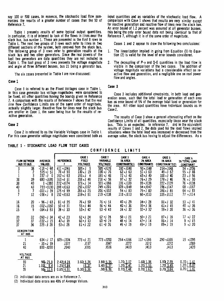
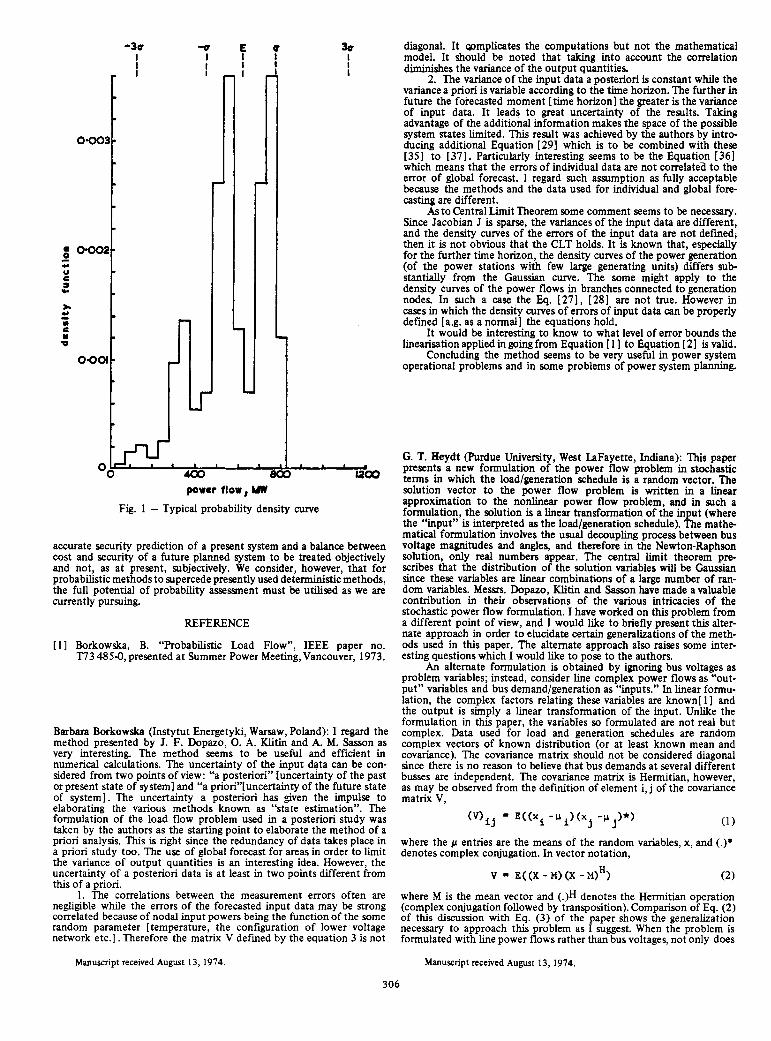
We would, however, like to comment on the author’s use of the Central Limit Theorem to assume that f 30 predicts satisfactory con- fidence limits. We, in a mutual collaborative effort between UMIST in England and the Institute of Power in Warsaw, have been currently investigating the same problem. We, however, not only characterise the power flows by expected values, standard deviations and confidence limits similar to that proposed by the authors, but also calculate the complete probability density curves of the power flows of interest. It was in order to calculate these density curves that the initial formulation, as described by Borkowskia,l. was limited to the d.c. case since these calculations are inherently complex.

in Fig. 1. This is clearly not a normal distribution and suggests that the One of our typical calculations produced the density curve shown

Central Limit Theorem does not apply. The difficulties arise because

whch is not necessarily the case when analysing typical power systems. the Theorem is only applicable for a large number of random variables

One consequence is illustrated in Fig. 1 where the value of the density function at a power level of E + u is nearly three times greater than at a power level of E.

limits enclose more than 99% of the probabilities of occurrence as We can c o n f m that all our results to date indicate that the k 30

assumed by the authors. We feel, however, that this could stiU lead to erroneous decisions if power flows of the type shown in Fig. 1 occur. In this example, the f 30 confidence limits enclose power levels between 100 and 1100 MW. Our results show, however, that the probability of power flows greater than 800 MW is neghgible. Therefore, with the authors’ confidence limits, the line could be almost 40% overdesigned.

objections may be raised concerning their accuracy. Preliminary work We accept our results were obtained using a d.c. representation and

using an a.c. model, however, indicates that the same trend prevails. In ending we would like to add our weight to the authors’ belief

that probabilistic assessment of system behaviour is necessary to enable

Manuscript received May 6,1974. Manuscript received August 7,1974

305

-30 I

i t d

-0 I w J L

E I I I ,

30 I I

I

1

oopl I ‘ 400 ‘ ‘ ‘ * 800 ‘ I ’ I ’ I200 a

power flow, MT Fig. 1 - Typical probability density curve

accurate security prediction of a present system and a balance between cost and security of a future planned system to be treated objectively and not, as at present, subjectively. We consider, however, that for probabilistic methods to supercede presently used deterministic methods, the full potential of probability assesanent must be utilised as we are currently pursuing.

REFERENCE

[ 11 Borkowska, B. “Probabilistic Load Flow”, IEEE paper no. 173 485-0, presented at Summer Power Meeting, Vancouver, 1973.

Barbara Borkowska (Instytut Energetyki, Warsaw, Poland): I regard the method presented by J. F. Dopazo, 0. A. Klitin and A. M. Sasson as very interesting. The method seems to be useful and efficient in numerical calculations. The uncertainty of the input data can be con- sidered from two points of view: “a posteriori“ [uncertainty of the past or present state of system] and “a priori“[uncertainty of the future state of system]. The uncertainty a posteriori has given the impulse to elaborating the various methods known as “state estimation”. The formulation of the load flow problem used in a posteriori study was taken by the authors as the starting point to elaborate the method of a priori analysis. This is right since the redundancy of data takes place in a priori study too. The use of global forecast for areas in order to limit the variance of output quantities is an interesting idea. However, the uncertainty of a posteriori data is at least in two points different from this of a priori.

1. The correlations between the measurement errors often are negligible while the errors of the forecasted input data may be strong

random parameter [temperature, the configuration of lower voltage correlated because of nodal input powers being the function of the some

network etc.] . Therefore the matrix V def i ed by the equation 3 is not

Manuscript received August 13, 1974.

diagonal. It complicates the computations but not the mathematical model. It should be noted that taking into account the correlation diminishes the variance of the output quantities.

2. The variance of the input data a posteriori is constant while the variance a priori is variable according to the time horizon. The further in future the forecasted moment [time horizon] the greater is the variance of input data. It leads to great uncertainty of the results. Taking advantage of the additional information makes the space of the possible system states limited. This result was achieved by the authors by intro- ducing additional Equation [29] which is to be combined with these [35] to [37]. Particularly interesting seems to be the Equation [361 which means that the errors of individual data are not correlated to the error of global forecast. I regard such assumption as fully acceptable because the methods and the data used for individual and global fore- casting are different.

As to Central Limit Theorem some comment seems to be necessary. Since Jacobian J is sparse, the variances of the input data are different, and the density curves of the errors of the input data are not defined, then it is not obvious that the CLT holds. It is known that, especially for the further time horizon, the density curves of the power generation (of the power stations with few large generating units) differs sub- stantially from the Gaussian curve. The some might apply to the density curves of the power flows in branches connected to generation nodes. In such a case the Eq. [27], [28] are not true. However in cases in which the density curves of errors of input data can be properly defined [a.g. as a normal] the equations hold.

linearisation applied in going from Equation [ 1 ] to Equation [ 21 is valid. It would be interesting to know to what level of error bounds the

operational problems and in some problems of power system planning. Concluding the method seems to be very useful in power system

G. T. Heydt (Purdue University, West LaFayette, Indiana): This paper presents a new formulation of the power flow problem in stochastic terms in which the load/generation schedule is a random vector. The solution vector to the power flow problem is written in a linear approximation to the nonlinear power flow problem, and in such a formulation, the solution is a linear transformation of the input (where the “input” is interpreted as the load/generation schedule). The mathe- matical formulation involves the usual decoupling process between bus voltage magnitudes and angles, and therefore in the Newton-Raphson solution, only real numbers appear. The central limit theorem pre- mibes that the distribution of the solution variables will be Gaussian since these variables are linear combinations of a large number of ran- dom variables. Messrs. Dopazo, Klitin and Sasson have made a valuable contribution in their observations of the various intricacies of the stochastic power flow formulation. I have worked on this problem from a different point of view, and I would like to briefly present this alter- nate approach in order to elucidate certain generalizations of the meth-

esting questions which I would like to pose to the authors. ods used in this paper. The alternate approach also raises some inter-

An alternate formulation is obtained by ignoring bus voltages as problem variables; instead, consider line complex power flows as “out-

lation, the complex factors relating these variables are known[ 1 ] and put” variables and bus demand/generation as “inputs.” In linear formu-

the output is simply a linear transformation of the input. Unlike the formulation in this paper, the variables so formulated are not real but complex. Data used for load and generation schedules are random complex vectors of known distribution (or at least known mean and covariance). The covariance matrix should not be considered diagonal since there is no reason to believe that bus demands at several different busses are independent. The covariance matiix is Hermitian, however, as may be observed from the definition of element i, j of the covariance matrix V,

where the p entries are the means of the random variables, x, and (.)* denotes complex conjugation. In vector notation,

v - E((X -M)(x -x)H) (2)

where M is the mean vector and (.p denotes the Hermitian operation

of this discussion with Eq. (3) of the paper shows the generalization (complex conjugation followed by transposition). Comparison of Eq. (2)

necessary to approach this problem as I suggest. When the problem is formulated with line power flows rather than bus voltages, not only does

Manuscript received August 13, 1974,

306

the mathematical treatment change, for example, E,q. (5) of the paper becomes

= (JH V-’ J)’l JH V-l Y.

but also the information derived changes. Line loading is obtained directly, and many of the power flow statistical inferences carefully described in this paper are also available. The advantage of the method of Messrs. Dopazo, Klitin and Sasson primarily lies in the availability of the Jacobian matrix. The advantages of the alternate formulation which

required) and certain other computational factors. I suggest primarily lie in the speed of computation (no inversion is

I would like to raise some questions of the authors in order to clarify some points. Why is covariance matrix V,

t V - E@, E )

treated as diagonal? Presumably, if the statistics of E are available, even cases where independence does not hold could be handled. Secondly, I would like to ask a difficult question concerning the accuracy of the calculation of the line flows (labelled z in the paper) by the method given by the authors. When the method described in the paper is used, a linearization is required to obtain bus voltage information @. (1) of the paper) and a sxond linearization is required in order to obtain the line flows (Eq. (18) of the paper). Would more accurate statistics of z be obtained by formulating the load flow problem directly with z as the independent variable rather than x? When this is done, onlyone lineari- zation is needed.

This paper presents a well written account of stochastic calcula- tions in power flow studies. I have no doubt that the results and tech- niques will be used by others to obtain many other useful statistical in- ferences of electric power system operation.

REFERENCE

[ 11 G. T. Heydt, B. M. Katz, “A Stochastic Model for Simultaneous Interchange Capacity Calculations,” to be published, IEEE Trans. on Power Apparatus and Systems.

K. F. Schenk and K. Singh (University of Ottawa, Ottawa, Ontario, Canada): This paper is another one of a series of papers which the authors have written in their systematic efforts to develop practical applications of statistical notions to the analysis of power system problems. This is a natural development when one recognizes that deterministic models and solutions do not fit well with real-type problems. Although deterministic results have a greater appeal than

meters, data and models. T h i s is, in our view, a step forward in the right stochastic results, the latter recognizes the impossibility of exact para-

direction. The authors are to be congratulated for their timely efforts.

variables, E, may be considered to be normally distributed as a conse- As is pointed out in the paper, the vector of ‘error’ random

quence of the Central Limit Theorem. This being the case, the estimators for x and ux2 (and for z and uZ2) may be obtained by maximizing the likelihood function. This is, of course, a well known fact, but it gives an

mum likelihood estimators (m2.e.) which are unbiased (not all of them additional insight into the formulation of the problem. Moreover, maxi-

are!) also exhibit some other properties which make them very desirable estimators: minimum variance, consistent, efficient, sufficient, complete and independent. Furthermore, under quite general regularity conditions on the density function[ 1 1 , any function u ( 2 ) of a m.!Z.e. 2 of i is the m.!2.e. of u(x).

meaningful results can be extracted from the method if it is properly In addition, it may be worthwhile to point out that useful and

applied. Only those cases which are considered normal with small data variations about an operating point will give useful results. Extreme variations in the input data (which are allowed by a normal distribution) may give uninterpretable results.

REFERENCE

[ 11 F. A. Graybill, “An Introduction to Linear Statistical Models”, Volume 1, McGraw-Hill, 1961.

Manuscript received July 2, 1974.

S. T. k p o t o v i c (Research Institute Nikola Tesla, Beograd, Yugoslavia): The authors have presented an interesting, useful and simple method for calculating the effect of the propagation of forecasted data inaccuracies through the conventional load flow. The method, using the principles of statistical least squares estimation for linear systems and addressing itself to the problem of processing the expected errors in the input data, that is, load bus P and Q, and generator bus P and E, converts the load flow problem formulation from a deterministic one to a stochastic one. The proposed method, through the extension of the conventional load flow problem, has included the calculation of the effects of inaccuracies in input data on all output quantities, namely on all bus state variables E and S or on line flow P and Q and generator bus Q. The stochastic load flow represents, in this way, the combined results of many deterministic load flows in which for each flow the data are perturbed, such that the various flows represent possible sets of data within the precision that the input data is known.

The model of the load flow in which a constraint on total system load plus losses has been placed by including a real power equation for the slack bus can be considered as a realistic one, since the forecasted errors are then distributed among generator P equations. It is to be believed, that further experience in using the developed method will make it simpler and more attractive.

The authors should be complimented for this nice paper.

Manuscript received August 13,1974.

A. Petroianu (National Center of Romanian Power System, Bucharest, Romania): The authors are to be commended for a thought provoking paper related to an interdisciplinary .in character problem.

The paper is devoted to the research problem of influence of initial data random errors upon the results of load flow calculation.

Such an investigation is very timely for the comparison of different mathematical models suitable for “off” and “on” line load flow calcula- tions.

The authors have a probabilistic approach to the problem of estimation of the results of calculation. From the probabilistic point of view the initial data should be considered as random variables with multidimensional distribution law.

We can underline two distinct direction of research in the frame of the probabilistic approach: 1 -Initial data errors are of stochastically definite nature

In this case the initial data are given by their mean value (mathe- matical expectations) and by their extreme limits of deviations (errors) from mean values. The law of distribution of initial data errors is supposed to be known.

It seems to the discusser that such an approach was used in[ 11. 2-Initial data errors are of stochastically i n d e f ~ t e nature

In this case only the extreme values of initial data errors are known. I believe that considering “a model in which all input data was

assigned error bounds” the authors are approaching a more practical way since the law of distribution of errors is often unknown.

In the frame of the probabilistic approach, considering that the deformation of the initial data is small, the knowledge of the expecta-

distribution law of the calculated values which constitutes our aim. tions and of the variance-covariance matrix sufficiently characterizes the

I would like to remark that a geometrical approach could introduce some fresh point of view that corresponds to the necessity of reducing

number of pertinent, synthetic and intuitive information [2 + 51. the great output data streams, generated by the computer, to a small

The geometrical theory, which can be conceived in parallel to the probabilistic approach, permits us to find and to describe an area of possible errors and the guaranteed region to which the calculated values belong.

where x, y are column vectors in m- and n- dimensional Euclidean spaces

y = y + i ; y (2)

where Sy- small random vector with variancecovariance matrix Ay. In accordance with the principle of linearization:

- = ‘t‘ (y) + a x (3 1

6~ = J L y .- (4)

Manuscript received July 30,1974.

307

where J Jacobian matrix for cp taken at the pointy. accordingly,

The variancecovariance matrix Ax for S x can be calculated

L

and characterizes the errors in the solution vector x due to the non- exactness in giving initial vector data - y.

quadratic form: XT 45 Formulae (5),corresponds to the general matrix expression of a

In the realm of an n-dimensional space with which is our present concern this quadratic form can be geometrically interpreted as repre- senting the area of the error hyperellipsoid.

Even under the simplifying assumptions that the admissible errors of x and y are sufficiently small to be related by the linear transforma- tion (4), the small region in which S y is contained is stretched in one direction and compressed in the other.

If the estimate of errors is made b the ctral vector norm, then the admissible regions for Sy will be an Kyperzpsoid.

If in turn we estimate 6x by the spectral norm we shall be forced to take as admissible the hypersphere with radius equal to the largest half-axis of the hyperellipsoid. This hypersphere will be larger than the hyperellipsoid; this replacement of the hyperellipsoid by the hyper- sphere involves the loss of information due to the uncertainty and errors in input data.

Formulae (5) expresses a hyperellipsoid which is in a skew position with respect to the oblique coordinate axes; by means of a suitable transformation to the principal axes of the hyperellipsoid the equation can be reduced to the canonic form

where &l . . .An are the eigenvalues. That is equivalent to consider only the variance of components

(i.e. ignoring the correlation coefficient); in this case we shall obtain the confidence hyperellipsoids with the axes being directed along the coordinate axes.

The degree in which the uncertainty of basic information is “conditioning” the uncertainty of the steady state solution is expressed by the square root of the ratio of the eigenvalue of maximal modulus to the eigenvalue of minimal modulus.

Formulae (7) which gives the elliptic norm (conditionality number),

can be geometrically interpreted as the ratio of the hyperellipsoid semiaxes.

By virtue of the above formulae it is evident that the precision, convergence and stability properties of the load flow solution are optimum for

H = 1,

that corresponds to the perfect symmetry of a hypersphere. The discusser’s comments, regarding the geometrical approach,

were intended to underline the importance of the authors’ contribution to a new emerging research problem - the probabilistic load flow

various existent schools of thought. problem - and to add some bits of information in an effort to relate

REFERENCES

[ 1 I Power System Computer Feasibility Study - 1968 - vol. I , IBM

[21 C. Lanczos, “Applied Analysis” Prentice Hall, 1956. [ 3 I A. Petroianu “A geometrical approach to the steady state problem

of electrical networks”. Rev. Roum. Sci. Techn.-Electrotechn. et

[41 V. I. Idelchik “About t k error influence of initial data upon the Energ., 14,4 p. 623-630, Bucharest, 1969.

result of power flows calculations in power systems” Izvestia, the USSR A.S. Energetics and Transport, 1968, No. 2, p. 9-15.

[ 5 1 D. K. Faddeev, V. N. Faddeeva “Stability in Linear Algebra Problems” A.F.I.P.S. Congr. 1972. Ljubliana.

Research Division, San Jose, California.

B. E Wollenberg (Leeds and Northrup Company, North Wales, Pa.): This is a very important paper. The techniques used in calculating the covari- ance matrices of system states and quantities computable from the states are definitely useful in all analytical studies requiring a load flow solution. I agree that any time a load flow is run, whether for real time studies or planning studies, a recognition of the data inaccuracies is al- ways useful - and necessary.

The authors have been careful to develop a technique which is used in conjunction with a conventional load flow solution and not a least squares state estimator type solution. The primary contribution of the paper is in showing how to compute the covariance matrices when adjustments such as area load or system total load, known to some specified accuracy, are placed on the solution. The authors correctly point out that such adjustments do not imply anything more than a con- ventional load flow solution. The covariance matrix calculations used to model the effects of the area or system load adjustments are correct for a least squares solution to the load flow with the area or system load values acting as redundant information. When a load flow is solved with the loads preadjusted to meet area or system conditions, the number of degrees of freedom remains the same and there is no filtering effect. A least squares solution with area or system load values as redundant information will produce filtering. The statement in the description of the authors’ Case 6 that ‘ I . . . there was no filtering effect caused by the redundancy of the slfck real power equation.” is somewhat misleading. It should have read . . . noapparent filtering. . .”, that is, there was no filtering which could be measured. In part thisis due to the fact that the error bound of 210 MW was allocated to the 14 generators by dividing 2 10 MW by 14 to give a 1 5 MW error bound. This calculation should have divided 210 MW by the square root of 14 which would have given a 56.1248 MW error bound for the generators. The 15 MW used by the authors was so much smaller than the 40% error band on the loads that

the 56.1248 MW error bound also and therefore shows that the covari- any filtering effect would be minimal. This result is probably true for

ance matrix calculation used is quite adequate.

Manuscript received August 2, 1974.

J. F. Dopazo, 0. A. Klitin, and A. M. Sasson: We are very pleased to the response of so many discussers to our paper and acknowledge their contributions to the subject. We are encouraged that in all cases the dis- cussers emphasize the need for treating the load flow stochastically.

which they calculate actual density curves with simplified models. We Messrs. Allan and Grigg and Ms. Borkowska present approaches in

consider that the distribution of input quantities, which is needed in their method, is generally not known. For instance, consider the

mentions. Over a period of a day the output of the plant can vary sub- generation of a large plant with several units which Ms. Borkowska

stantially and a non-normal distribution could be determined. However, the distribution of plant output at peak system conditions at some future year can be considered as a normal distribution with a small variance that depends significantly on what the distribution of the

upon the applicability of the Central Limit Theorem. The reasoning system peak is. The same discussors and Dr. Duran, express reservations

given for the distribution of input quantities also apply here. Line flows near generating plants, which is the example mentioned by Ms. Borkowska, can thus be considered as normal. Dr. Duran finds some

We agree that results are only approximately normal in the sense chi-squared component in the output when no linearizations are made.

approaches a normal as the degrees of freedom increases which justifies Dr. Duran points out. However, the chi-squared distribution rapidly

really after the bounds of output quantities and not their distribution. our use of the CLT for practical purposes. On the other hand, we are

are further justified. The unknown but bounded theory (9) applies here and our procedures

The arguments given above apply to a large extent t o the comments made by Messs. Heydt and Semlyen and Ms. Borkowska on the use of a diagonal input convariance matrix. Even in the case of P, Q values at the same bus which Dr. Semlyen refers to, while the variations during a day

for system peak conditions are considerably less so. are strongly correlated our expectation of P and Q at some future year

Messrs. Schenk, Sigh, Semlyen and Duran and Ms. Borkowska ask on the accuracy of results for large input variances, given the lineariza- tions involved in our method. Obviously, one can not expect to increase input variances indefinitely without serious deterioration in the accuracy. We would advise that tests similar to the ones we performed be made to answer this question for a specific system. If Monte Carlo load flows results can be reasonably duplicated by the stochastic load flow, then the latter applies for that level of input variances.

Manuscript received November 4,1974.

308

We were pleased to find the comments made by Ms. Borkowska and Dr. Despotovic on our differentiation between global and individual forecasts and the inclusion of total load error as variances over all generators thus eliminating the need for defining a slack bus. On this point, Mr. Wollenberg feels that our calculation of individual generator variances is in error. Considering a total load error bound of 210 to be spread over 14 generators he considers that the sum of the variances of generators should be equal to that of the total. Thus,

What we do is to divide the 210 evenly among the 14 generators. With Mr. Wollenberg’s suggestion we would be considering load flow situa- tions in which generation exceeds the bounds of total system load thus being unrealistic.

Dr. Heydt briefly presents a method he has developed in which he states there are some computational advantages. We understand that he will be presenting his method in a paper that will be presented shortly and we would like to reserve our comments until we read his forth- coming paper and understand his approach better. We will only point

out that the use of sparsity techniques makes our method computation- ally attractive.

We appreciate Dr. Petroianu’s comments on our paper and his geometric interpretation of the mapping of input errors to output quantities.

Dr. Duran’s derivation of the paper’s equations are the same as ours. We “complicated” matters by trying to show the relation between the theory of state estimation and that of stochastic load flows to emphasize that historically the idea of the latter came from the former.

We fmd Dr. Duran’s error analysis quite enlightning However the last term of the exact formula for the variance of G should be 2 RZup4 and not 2 R2o 2. This makes the errors in the mean and variance to be Rup2, and 2 R s 4 which are second order effects in their respective equations. For ins%nce, consider as an example that per unit Rand P are equal to 1 and an error bound for P equal to 0.3. This makes Op2 = (0.3/3)2 = 0.0 1. Then, the error in the mean and variance of G are 0.0 1 and 0.0002 while our computed mean and variance are 2 and 0.9 respectively.

REFERENCE

[9] F. C. Schweppe “Uncertain Dynamic Systems,” Prentice-Hall Inc., Englewood Cliffs, N. J., 1973.

309