Embed Size (px)
Citation preview

r i
r ' '
I
!
\\ L.,
T. J. Wipf, F. W. Kl.allier, D. M. Besser, M. D. LaViolette
Manual for Evaluation, Rehabilitation and . Strengthening of Low Volume Bridges
~t.. Iowa Department "'l of Transportation
Februacy 1993
Sponsored by the Iowa Department of Tra!lSportation and the
Iowa Highway Research Board
Iowa DOT Project HR-323 ISU-ERI-Ames-93062
..... College of Engineering
Iowa State University

!
(' )
T. J. Wipf, F. W. Klaiber, D. M. Besser, M. D. LaViolette
Manual for Evaluation,. Rehabilitation and Strengthening of Low Volume Bridges
Sponsored by the Iowa Department of Transportation and the
Iowa Highway Research Board
Iowa DOT Project HR-323 · ISU-ERl-Ames-93062
\; i '~
J· ;~en ineeri~g researc institute
iowa state university

Tue opinions,. findings, and conclusions expressed in this publication are those of the authors and not necessarily those of the Highway Division of the Iowa Department of Transportation.

ill
.ABSTRACI'
This report contains an evaluation and design manual for strengthening and replacing low volume steel
stringer and timber stringer bridges. An advisory pane( consisting of county and municipal engineers provided
direction for the development of the manual NBI bridge data, along with results from questionnaires sent to
county and municipal engineers was used to formulate the manual
Types of structures shown to have the greatest need for cost-effective strengthening methods are steel
stringer and timber stringer bridges. Procedures for strengthening these two types of structures have been
developed. Various types of replacement bridges have also been included so that the most cost effective
solution for a deficient bridge may be obtained.
The key result of this study is an extens~ compilation, which can be used by county engineers, of the
most effective techniques for strengthening deficient existing bridges. The replacement bridge types included
have been used in numerous low volume applications in surrounding states, as well as in Iowa. An economic
analysis for determining the cost-effectiveness of the various strengthening methods and replacement bridges
is also an important part of the manual Microcomputerspreadshee1 software for several of the strengthening
methods, types of replacement bridges and for the economic analysis has been developed, documented and
presented in the manual So the manual, Chp. 3. of the final report, can be easily located, blue divider pages
have been inserted to delineate the manual from the rest of the reporL

v
Tab1c Of Conllmlll Page
Abstract • . . • • . . • • • . • . . . . • . . . . • • . . • • . . • • . . . • . . • . . . . . • • . . . . . . . • • . . . • . . • . . . . . . . . . . . iii I
List of Figures ..••••.••••••••.........••.•••..••••••••••••••••••..•••••.••.•...••. ix
List of Tables •..•••..•••.••..••.......••.•••••..••••..........•.....•............. xi
1. .Introduction and Research Approach . . . • • • . • • . . • • • . • . • . . . . • • . . . . . • . . . . . • . . • . . . . . . . 1
1.1. Background . . . . . . • • • . • • . . • • . . . . • . • • • . . . • . • • . • • . . • • • . . . . • . . . . . . . . . . . . . . . . 1 1.2. Research Objectives • • • • • • • • • • • • • • • • • • . • • • • • • • • • • • • • • • • • • • • . • • • • . • • • • • • • • • • 1 1.3. Scope of Investigation • . • • • • • • • • . . • • • • • • • • • • • • • • • • • • . • • • . . • • • • • • • • . • • • . . . . . • 2 1.4. Research Approach • . • • . . . • • . • .. . • . • • • . • • • . . . . . . . . . . . . . • . . • . . . . • • • . . . • . .. . 4
1.4.1. Task 1 ••.•...••.•..•••.•.••..•....•..•••.••••...•....•..••.•....•. 4 1.4.2. Task 2 . .. . . • • • . • • • • . • .. . . • • • • . • . . . . • . . . . • • . . . . . . . . . • . . . • . . . . . . . .. . 4 1.4.3. Task 3 • . . • . . . . . . . .. . . .. • • • . . .. . . . . . .. . .. . . . . • . . . . . . . . • . . • • . . . . . . . . 4 1.4.4. Task 4 . . • • • . • • • . . • • • . . • • • • • • • • • • • • . . • • • • . • • • . • . • • . . . • . . . • . . . . . • . . . 4 1.4.5. Task 5 ••••••••••.••••.••••••••.•••••.•••..•••••••••.••..••.....••• 5 1.4.6. Task 6 . • • . . . . . • . . . . . . . . • . • • • . • • . • • • . . .. . . • • • . . . . . . . . • . . . . . . . . . . .. . 5
2. Findings . . . • • . . . . . . . . . . . . . . . . . . . . . . . . . . . . • . . . • . . . . . . . . . . . . . . . . . . . . . . . . . . . . . . 7
2.1. Panel Meetings ...•.•........•....•....•............•• : . . . . . . . . • . . . . . . .. . 7 2.2. National Bridge Inventory ............ · ...•...•...•....••..••...•.•..•......•. 7 2.3. Questionnaire Results ...••...•....•. ~ . . • • . • . . . . . . . . . . • . • . . . • • . . . . . . . . . . . . . 16 2.4. Literature Review ..•....••.•..••...•.........••..••........• : . . . . . . . . . . . 22
2.4.1. Oeneral • . . . . • . . . . . • • . . . . . . . . • . . . • • . . . . . . . . . . . . . • . . . . . • . . . . . . . . . . . 22 2.4.2. Timber Bridges . . . . . . . . . . . • . . . . . . . . . . . . . . . . . . • . . . . . . . . . . . . . . . . . . . . . 23 2.4.3. Steel Bridges . . . . .. . . • . • . . . • • . . . • • . . .. . .. • • . . . . . . . . • . . . . • . . . • . . . . . . 24 2.4.4. Cost Effectiveness Studies . . . . . . . • . • . . . . • . . . . . . . . . . . . . . . . . . . . . . . . . . . . . 26
3. Applications . . . . . . • • . . . . • . . . • . . • . . . . • • . . • • • . . . . . . . • . . . • . . . . . . . . . . . . . . . . . . . . . 31
3.1. General Information-. ........••.••.••.•.••.•••....••..•.•................. 31 3.1.1. Background .........•••..•••.•••..•...•....••...•.•...•........... 31 3.1.2. Scope of Manual . • • • . . • . • • . . • • . . • . • . • • . . . . . . • • . . . . . • . . • • • . . . . • . . . • . 36 3.1.3. Use of Manual . . • . . . • • . . . . • • . . . . . • . . . . . . . . . . . . • • • • . . . • . . • . . . • . . . . . 37
3.1.3.1. Applicable Strengthening Techniques for fllWA 302 Bridges ..•...•... 38 3.1.3.2. Applicable Strengthening Techniques for F1:lW A 702 Bridges . . • . . . . . . . 38 3.1.3.3. Replacement Bridges ...•••.............. , . . • . . . . • . . . . . • . . . . . 38 3.1.3.4. Microcomputer Spreadsheets .•.••.••..• ~ .. .. . • . . . • . . • . . . . . . . . . 39
3.2. Inspection ............................................................ ·. . 41 3.2.1. Decks . . • • • . . . . . . . . . . . . • • • . . . . . . . • . . . . . . . . . . . . . . . . . . . .. . . . . . . . . . . . 42 3.2.2. Stringers/Beams . . . . . . . • . . . . . . • .. . . . . . . . . . .. . . .. . . • . . . . • . . . . . . . . . . . . 44 3.2.3. Drains, Bearings and Expansion Joints • . . . . . . . . . . . . . . . . . . . . . . . . . . . . . . . . . . 45
3.3. Fundamentals . . . . . . . . . . .. • • . . . • . . . . . • • . . . • . . • . . . .. . . .. • . . .. . . . . . . . . . . . . . 46 3.3.1. Dimensions . • . • . . . . . • • . . . . . . • . . . . • . . . . . • • . . • • . . . . . . . • . . . . . . . . . . • . . 46 3.3.2. Materials (Allowable Stresses) .•...••..............•................... 46
3.3.2.1. Steel . . . . . . . . • . • . . . . • . . • . • . . • . • . . . • . . . . . . . . . . . . . • . . . . . . . . . 46 3.3.2.2. Timber . . . . . . . . . . . . . . • . . . • . • . . . . . . • . . . • . . . . . • . . . . . . . . . . . . . 47

3.3.3. 3.3.4. 3.3.S. 3.3.6.
vi
Page
Loads . . . . . . • . . . • • . . . • • • . . . . • • . • . . • • • • • • • .. • • . . . . . . . • . . . . • • . . . . . . 48 Condition . . . • • . . . • • . • . . • . • • • • • • • • • . • • • . . • • • . . • . . . • . . . . . • • . • . . . • . • • 51 Rating ..•...•..•••. , . . . . • . . . • • • • • • . . . • • . • • . • • . • . . . . . . . . . . . . . . . . .. . 52 Examples • • . . . . . • • . . . • • • • • • • . • • • . . . • • • • • • • . . . . . • . . . .. .. . . . . • . . . . • . 54 3.3.6.1. Example 1: Timber Stringers (1 ft-0 in. on center);
timber deck with rock fill • .. . . • • . . • • . . . • .. . . . . • . . . . 54 3.3.6.2. Example 2: Timber Stringers (1 ft-0 in. on center);
timber deck • • • • • • • • • . • • • • • • • . . • . . • . . • . . . . . . . . . . 57 3.3.6.3. Example 3: Timber Stringers (1 ft-2 in. on center);
timber deck with rock fill • . . • . . . . • • . . . • .. . . . .. .. .. . 59 3.3.6.4. Example 4: Steel stringers with full lateral support
of compression tlange • • • . . . • • . . . . . . . . . • • . . . . . . . . . . 62 3.3.6.S. Example 5: Steel stringers with lateral support of
compression tlange at 10 ft interva!S . . . • • . . • . . . . . • . . . . 65 3.3.6.6. Example 6: Steel stringers with full lateral support
3.3.6.7. 3.3.6.8. 3.3.6.9. 3.3.6.10.
Example 7: Example 8: Example 9: Example 10:
of compression tlange and holes in bottom flange . . . . . . . . 67 Rating of timber deck (4 in. x 12 in.) ••..••..••......• 73 Rating of timber deck (3 in. x 12 in.) • • . . • • • . . • . • . . . . . 77 Rating of laminated timber deck (2 in. x 4 in.) .•.....•.. 79 Rating of layered timber deck • . . . . .. . . . .. • . . . . . . . . . . 81
3.4. Economic Analysis . . . . . .. . . . . .. . . .. .. . .. . . . . . . . . . . .. . . . .. . . . .. . . . . . . . . . . . 86 3.4.1. Background • • . • • . . • • • . . • • • • • • . . . . • • • • . . . • • . . . . • . . . . . . . . . . • . . . . • . . . 86 3.4.2 Description of Analytical Model . .. • • .. . . . • .. . . . .. . . . . . • . . . .. . .. . . • .. .. . 87
3.4.2.i. Replacement Structure FJrst Cost (R) . . • • • . . . • . . . . • . . . . . • . . . . • . . . 91 ·3.4.22. Structure Service Life (N,N') • . • . . . . . • . . . . • . .. . . .. . .. . . . . . . . . . . 91 3.4.23. Interest Rate (i) • • . . . • • • • • • • • . • • • . . . • • • • . . . . . . • . • . . . . • . . . . . . 91 3.4.2.4. Bridge Maintenance Costs (C.nC..) • • • • • • • • • • • • • • . . • • • • . . • • . • . . . . 92 3.4.2.5. Bridge Removal Costs (B,S) • . . . . . . • • . . . . • • . . . . . . . . • . . . . . . . . . . . 92 3.4.26. Level of Service Factor (LS) • . • • . . . . .. . • . . • • . . . . . . . . . . . . . . . . . . . 92 3.4.2. 7. Other Considerations • • • . . . • . . • . . . . • . • . . • . . . . . . . . . . • . . . . . . . . . 93
3.4.3. Normal Distnoution and EUAC Simulation . • • . . . . • • . . . • • . . . . . • . . . . • . . . . . . 93 3.4.3.1. Normal Probabilily Distnoution • . . • • • • • . . • • • . • • • .. • . . • . . . . • . . . . . 93 3.4.3.2 Simulation of EUAC Results • • • • • . • • • • • • . • • • • • • • • • . • • • • • • • • . . . • 95
3.4.4. Computer Spreadsheet for EUAC Comparison • • • . . • • . • • • • • . . . . . • • . • . . . . . • . 95 3.4.S. EUAC Example • • • . • • • • • • • • • • • . • • • • • • • • • • • • • . • • • . . . • • . . . . . • . . . . • . . . 96
3.5. Strengthening Techniques for Steel Stringer Bridges (FHW A 302) . . . . . . . . . . . . . . . . . . . • 99 3.5.1. Replacement of Damaged Stringers . . • • • • • . . . • • • • . .. . • • . . . . .. . . • . . . . . • . . 99 3.5.2. Respacing Existing Stringers and Adding New Stringers • • . . . . . . . . . . • . . . . . . . . 101
3.5.2.1. Background • ; . . • • • . . . . . . • • • . • . . . . . . . • . . . . . . . . . . . . • . . . . . . . 101 3.5.2.2 Design Criteria . • • . • . • • . . . . . . • • . • • . . . . . . . . . . . • . • . . . . • . . • • . . 101 3.5.23. Design Limirations . . . . . • • • . . . . . . . • • . • . . . . . . . . . . . . . . . . . . . . . . 101 3.5.2.4. Design Procedure . . . • • • . . . • • . . . . • . . . . . . . . . . . . . . . . . • . . . . . . . . 102 3.5.2.5. Evaluation of Existing Stringers Example . • . . . . . . . . . . • . . . . . . . . . . . . 105 3.5.2.6. Respace and Add Stringer Example . . . . . . . . . . . . . . . . . . . .. . . . . . . . 109
3.5.3. Increase Section Modulus . . . • . . . . . . . . . . • . . • . . . . . • . . . . . . . . . . • . . . . . . . . . 109 3.5.3.1 Background . . . . • . . . • . • • • • • • . • . . . . . • . . . . . . . . . . . . . . . . . . . . . . 109 3.5.3.2. Increased Section Modulus Example . • • . . . . . . . . . . . . . . . . . . . . . . . . . 111
3.5.4. Develop Composite Action ...... ·. . . . . . . . • . . . . . . • . . . . .. .. . .. • . . . . . . . . . 111
j
\ . ...._,JI

vii
Page
3.5.5. Deck Replacement . • . . . . • • . . . • • • . • . • • . . • • . • . • . . . . . . . • • . • . . . . • . . . • • 114 3.S.6. Post-Tensioning . • • . . . . . . . . . . . • • • . . • • • • . • . • . • • • . • • . . . • • . . . • . . . . . . . • 114
3.5.6.1. Background . . . • • . . . • . • • • . . • • • • • . • • • . • • . . . . . . • • • • . . . • • . . . . 114 3.5.6.2. Post-TensioningExample .................................... 115
3.6. Strengthening Techniques for Timber Stringer Bridges (FHW A 702) • • • . • • • • • • . • • . • • . 120 3.6.1. Respace Existing Stringers and Add New Timber Stringers ...•••...••..••.••• · 120
3.6.1.1. Background • • . . . • • • • . • . • • • . • . • • • • • • • • • • • . . • • • . . . • • • . . . . . • 120 3.6.1.2. Design Criteria • • . • • . . • • . . . • • • • • • • • • • • • • • • . . . . . • . • . • . . • . • . . 120 3.6.1.3. Design Limitations . . • • • • . • • • • . . • • . • . • . . . . • . . • • • • . . • • . . • • • • • 120 3.6.1.4. Design Procedure • . • • . • • • . . • • • • • • • • . • • • . • . . . . . . • . • . • . . . . . . . 125 3.6.1.5. Respace and Add Timber Stringers
Example: Spacing = 2 ft - Case I .. • • .. .. • .. • . . . .. • .. .. . . . .. .. • 127 3.6.1.6. Respace and Add Timber Stringers
Example: Spacing = 1 ft - Case II • . . • • .. .. • .. • . . .. • .. • . • • .. . .. 130 3.6.2. Replace Limited Number of Timber Stringers with Steel Stringers . . . . . . . . . . . . . 130
3.7. Replacement Bridges . • . • . . • . . . . • . • . . • • • . . • • . . • • . . • • . . . • • • . • • • . . . . . . . . . . . 134 3. 7.1. Precast Culvert/Bridge . . . . . . . . . • . . . • • . . • • . . . . . . . • . . . . . . . . . • . . . • . . . . . 138
3.7.1.1. Background . . . . . . . • . . . . • • . . . • . . . • . . . • . . . . . . . . • • . . . . • . . . . . 138 3. 7.1.2. Design Criteria . • . . . . . . . . . . . . . • . . . . . . . . . . . . . . . . . • . . . . • • . . . . 138 3.7.1.3. Design Requirements . . . . . . . . . . . . . . . . . . . . . . . . . . . . . . . . . . . . . . . 138 3.7.1.4. General Cost Data • . . . . . . . . . . . • • . . . . • . . . • . . . . . . . . . . . . . . • . . . 140 3.7.1.5. Cost Information: Case Studies . . . . . . • . . • • • . . . . . • . • • . . . . • . . . . . 141
3.7.2. Air Formed Arch Culvert . . • . . . . . • • . . . • . . . . • . . . . . . . . • . . . . . . . . . . . . . . . . 141 3.7.2.1. Background . • . • • . . . . . . . . • . . . • . . . • . . . • • . . . . . . . . • • . . . . . • • . . 141 .3.7.2.2. Cost Information: Case Study. • . . . . . . . . • . . . . . . . • . . . . . . • • . • . . . . 142
3.7.3. Welded Steel Truss Bridge .•..........•...•...•...••................• 142 3.7.3.1. Background .............•.......•...••.........•......... 142 3.7.3.2. Cost Information: Case Study . . . . . . • . . . • . . . . . . . . . • . . . . . . . . . . . . 145
3.7.4. Prestressed Concrete Beam Bridge .. . . .. . .. • . . .. . . . . • . . . . . . . . . . . . . .. . . . 145 3.7.4.l. Background . . . . . . • . . . . • . . . . • . . . . . . . • . . . . . . . . . . • . . . . . . . . . . 145 3.7.4.2. Design Criteria . . . . . . . . • . . . • . . . . . . . • • . . . • . . . . . . . . . . . . . . . . . . 148 3.7.4.3. Cost Information: Case Study . . . • . . . • • . . • • . . . . . . . . . • . . . . . . . . . . 150
3.7.5. Inverset Bridge System . . • • • . . . . . . . . . . . . . • . . . . • . . • . . . . . . . . . . • . . . . . . . . 150 3.7.5.1. Background . . . . . . . . . . . . . . . . . . . . . . . . . . . . . . . . . . . . . . . . . . . . . . 150 3.7.5.2. Example • . . . . . . • . . . . . . . . . . . • . . . . . . . . . . • . . . . . . . . . . . . . . . . . . 152 3.7.5.3. Cost Information: Case Study ..........•.•............•....... 158
3. 7.6. Precast Multiple Tee Beam Bridge ...••.•............. ; . . . . . . . . . . . . . . . . 159 3.7.6.1. Background . . . • • . . . . . . . • . . . . . . . . . . . . . • . . . . . • . . . . . . . . . . . . . 159 .3.7.6.2. Cost tnformation: Case Study . . • . . . . . . . • . . . . . . . . . . . . . . . . . . . . . . 161
3.7.7. Low Water Stream Crossing. • . . . • . . . • . . . • . . . . . . . . . . . . . . . . . . . . . . . . . . . . 161 3.7.7.1. Background .•.................•......•....•.............. 161 3.7.7.2. ·Design Criteria . . . . . . . . . . • • . . . • . . . . . . . . . . . . . . . . . . . . . . . . . . • . 163 3.7.7.3. Costlnformation: Case Study ..........•..................•... 163
3.7.8. Corrugated Metal Pipe Culvert. . • • . . . . • . . . . . . . • . . . . . . . . . . . . . . . . . . . . . . . 165 3.7.8.1. Background . . . . . . . . . . . . . . . . • . . . . . . . . . . . . . • . . . . . • . . . . . . . . . 165 3.7.8.2. Design Criteria . . . . . . . . . . . . . . . . . . . . . . . . . • . . . . . . . . . . . . . . • . . . 166 3.7.8.3. Design Information . . . . . . . . . • . . . . . . . . . • . . . . . . . . . . . . . . . . . . . . . 167 3.7.8.4. General Cost Information . . . . . . . . . . . . . . . . . . . . . . . . . . . . . . . . . . . . 168
3.7.9. Stress-Laminated Timber Bridge . . . . . . . . . . . . • . . . . . . • . . . . . . . . . . . . . . . . . . 168

viii
3.7.9.1. Background ......•..••••••••.••••.•.••••...••.••...•....• 3.7.9.2 Design Criteria ••.....•..•••.•.•.••••...................... 3.7.9.3. General Cost Data ••..••..•••••..•••...................•... 3.7.9.4. Design Llmitations ....••••••.•••..•••...........•....•..... 3.7.9.5. Design Procedure .......•••••••..............•..••......... 3. 7.9.6. Example ••••••••••.•••••••••••.........•...••............
3.7.10. Glue-Laminated Timber Beam Bridge ..•.••••••.•••......••.••....•... 3.7.10.1. Background .•.....•.•.•••.•.•••.•.......•................ 3.7.10.2 Design Criteria ••••••.....•.•..••••..•.•................... 3.7.10.3. Design Procedure ..•.•••..••.•.•••••.........•..•.••..•.... 3.7.10.4. Example •.•..••.••••••••••...••••••.••..••.•.............
3.7.11. Glue Laminated Panel Deck Bridge .................................. . 3.7.11.1. Background ••••••••••••..................•.•..•....•..••. 3. 7.11.2 Design Criteria ....•................•..........••..•..•.... 3.7.11.3. Design Procedure .........................•........•....... 3. 7.11.4. Example ...••...•••..•••..•..•...•••..•..•.•..•..•.......
4. · Summary and Conclusions .................................................... .
4.1. Summary •............••...••••••..• ' .....•.....•.••....•............. 4.2 Conclusions .......................................................... .
5. Acknowledgments ...........••....••.•••.•...••••...•......•...•.....•......
6. References .......•........•••....•..•...................•.....• : ......... .
Appendix A: Iowa Legal Trucks ................•......•......•.....................
Appendix B: Live Load Moments .................................... · .............. .
Appendix C: Questionnaire Document. .............................................. .
I
Page ,,_JI
I I
168 169 172 173 175 191 198 198 200 203 214 223 223 225 225 237
245
245 245
247
249
255
259
267

Fig. 2.1.
Fig. 2.2.
Fig. 2.3.
Fig. 2.4.
Fig. 2.5.
Fig. 2.6.
Fig. 2.7.
Fig. 2.8.
Fig. 3.1.
Fig. 3.2.
Fig. 3.3.
Fig. 3.4.
Fig. 3.5.
Fig. 3.6.
Fig. 3.7.
Fig. 3.8.
Fig. 3.9.
Fig. 3.10.
Fig. 3.11.
Fig. 3.12.
Fig. 3.13.
Fig. 3.14.
Fig. 3.15.
Fig. 3.16.
Fig. 3.17.
Fig. 3.18.
Fig. 3.19.
Fig. 3.20.
Fig. 3.21.
Fig. 3.22.
ix
List of Ffgurea Page
Iowa county bridges by structure type •••••••••••••••••••••••••••••••••••••••• 9
Iowa municipal bridges by structure type • • • • • • • • • • • • • • • • • • • • • • • • • • • • • • • • • • • • • 10
Structurally deficient county bridges by structure type • • • • • • • • • • • • • • • • • • • • • • • • • • • 11
Structurally deficient municipal bridges by structure type • • • • • • • • • • • • • • • • • • • • • • • • • 12
Functionally obsolete county bridges by structure type • • • • • . • • • • • • • • • • • • • . . • • . • • • 14
Functionally obsolete municipal bridges by structure type • • • • • • • • • • • • • • • • • . • . . • . . • 15
Experience oflocal agencies with bridge strengthening and replacement . • • . . . . • • • . • . 17
Reasons for not implementing strengthening • • . . . • . • • . • • • • . . . . . . . . • • • . . . . • . • . . 18
Lengths of steel stringer bridges: FHW A 302 • • • • . . • • • • • • • . . . . • • • • • • • • . . • • . • • • 32
Widths of steel stringer bridges: FHW A 302 • • • . • • . • • • • • • • • . • • . • • • • • • . • • • . . . • 33
Design toad cases: FHW A 302 • • • • • • • • • • • . • . . • • • • • • • • • • • • • . • • • • • • • • • . • . . . . 34
Design H load cases: FHW A 302 • • • • • • • • . . . . . . • . • • • • • • • • • . . . • • • • . • • • . . • • . . 35
Example spreadsheet . . . . . . . . . . . . . . • . . . . . • . . . . . . • . . . . . . . . . . . . . . . . . . . . . . . 40
AASHTO standard loads . . . . . . . . . . . • . . . . . • . . . . . . . . . . . . . . . . . . . . . . . . . . . . . . 49
Iowa legal loads ............................................... , . . . . . . . . SO
Economic modelforreplacement alternatives . • • . . • . . . . . . . . . . • • . . . . . . . . . . • . • . . 88
Economic modelfor strengthening altema lives • • • • • • • • • • • • • • • • • • • • • • • • • • • • • • • • 89
Normal probability distnoution . . . . . . . • . . . . . . . . . . . . . . . . • . . . . . . . . . . . . . . . . . . . 94
Economic analysis spreadsheet, input parameters, and example problem . . . . . . . . . . . . . 97
Steel beam replacement • . . . . . • • . • . . . • . . . . . . . . . . . . . . . . . . . . . • . . . . . . . . . . . . 100
Spreadsheet for steel beam replacement example . . . . . . . . . . . . . . . • • . . . . . . . . . . . . 106
Example bridge: red1·~tion of stringer spacing • • . . . . . . . . . . . . . • • . . • . • • . . . . . . . . . 110
Addition of L and WI" sections . . • . . . • • . . • • • . . . • . • . . . . . . . . . . . • . • • . . . . . . . . . 112
Spreadsheet for increa5ed section modulus example . . . . . . . . . . . . . . . . . . . . . . . . . . . . 113
Spreadsheet for determining force fractions and moment fractions • . . . . . . . . . . . . . . . . 116
Spreadsheet for FF and MF example problem . . . . . . . . . . • . . • . . . . . . . . . . . . . . . • . . 121
Spreadsheet for timber stringer example. • . . . . . . . . . . . . . . . . . . . • . . . . . . . . . . . . . . . 128
Spreadsheet for timber stringer respace and add example . . . . . . . . . . . . . . . . . . . . . . . 131
Position of steel stringers in two lane and single lane bridges . . . . . . . . . . . . . . . . . . . . . 132
Maximum longitudinal stress in timber stringer: Bridge width = 24 ft;
Stringer size = 4 in. x 12 in.; Stringer spacing = 12 in. . . . . . . . . . . . . . . . . . . . . . . . . . 133

Fig. 3.23.
Fig. 3.24.
Fig. 3.25.
Fig. 3.26.
Fig. 3.27.
Fig. 3.28.
Fig. 3.29.
Fig. 3.30.
Fig. 3.31.
Fig. 3.32.
Fig. 3.33.
Fig. 3.34.
Fig. 3.35.
Fig. 3.36.
Fig. 3.37.
Fig. 3.39.
Fig. 3.40.
Fig. 3.41.
Fig. 3.42.
Fig. Al.
x:
Page
Maximum longitudinal stress in steel stringers: Bridge width = 24 ft;
Stringer size = 4 in. x 12 in.; Stringer spacing = 12 in. • • • • • • • • • . • • • . • • . . • . . . • . • 135
Maximum longitudinal stress in steel stringers: Bridge width = 24 ft;
Stringer size = 4 in. x 12 in.; Stringer spacing = 12 in. • . . . . . . . . . • • . . . . . . . • . . • . . 136
Displacements in timber and steel stringers: Bridge width = 24 ft;
Stringer spacing = 12 in.; Bridge span = 18 ft; Stringer size = 4 in. x 12 in. 137
Con-Span precast bridge segment • . . . . . . • • • . . • • . . . . • . . • . . . . . . . . . . . . . • . . . . . 139
U.S. bridge welded steel truss bridge • • • . • • • • • • . • • • • • . . . • . . . . • • • • . . . . . . . . . . . 143
Standard prestressed concrete beam shapes • • • . . . . . • • • • . . • . . . . . . • • . . . • . . . . . . . 146
Standard prestressed ooncrete double-tee bridge girder • . . . . . . . . . . . . . . . . . . . . . . . . 149
Inverset bridge section during fabrication •.............•............... '. . . . . . 151
Longitudinal joint details for Inverset bridge . . . . . . . . . • . . . . . . . . . . . . . . . . . . . . . . . 157
"OK" precast multiple tee beam section . . . . • . . . . . . . . . . . . . . • . . . . . . . . . . . . . . . . . 160
Original stresslam bridge deck configuration .......••............... , . . . . . . . . 170
Stresslam configuration for new construction .......•........•......•. ·. . . . . . . . 171
Stresslam timber deck spreadsheet, input parameters, and example problems . . . . . . . . 176
Dimensions required to determine k factor • . • . . • • • • • . • . • . . . . . . • . • • . . . . . .. . . . . 190
Typical section of glulam timber beam bridge . • . • • • . . . . . . . . . • . • . . • . . . . . . . . . . . 199
Glulam tL.-nber beam spreadsheet, input parameters, and example probletr..s . . . . . . . . . 204
Dead load vertical shear load configuration . • • • . . . . • . • . . . . . . . . . • . . . . . . . . . . . . . 220
Live load vertical shear load configuration . . . . . . . . . . . . . • . . . . . . . . . . . . . . . • . . . . . 221
Typical section of glulam timber deck bridge . . . . . . . . . . . . . . . . . . . . . . . . . . . . . . . . . 224
Glulam timber deck spreadsheet, input parameters, and example problem • . . . . . . • . . . 226
Iowa Department of Transportation legal dual axle truck loads • • . . • • • . • . • • • . . . . . • 257
\ /' "-, I
j I I
\ I
I )
'

Table 21.
Table22
Table23.
Table 3.1.
Table.3.2
Table 3.3.
Table 3.4.
Table 3.S.
Table 3.6.
Table 3.7.
Table 3.8.
Table3.9.
Table3.10.
Table 3.11.
Table 3.12
· Table 3.13.
Table 3.14.
Table 3.15.
Table 3.16.
Table 3.17.
Table 3.18.
Table 3.19.
Table 3.20.
Table 3.21.
Table3.22
Table 3.23.
Table 3.24.
Table 3.25.
Table 3.26.
Table 3.27.
Table 3.28.
Table 3.29.
xi
List of Tables
Page
FHW A bridge codes . . • • . • . . . . . . . • • • • • . • . . . . • • • • • • . . • . . . . . . . . . . . . . . . . . . • 13
Summary of Section 2 questions . . . • • • • . • . • . • • • . • • • • . . • • • . . . • . . . . . . . . . . • . . • 19
Summary of services for which agencies employ consultants . . . • . . . . . . . . . . . . . . . . . • . 20
Contents of design manual listed by primary sections . . . . • . . . . . . . . . . . . . . . . . . . • . . . 37
Spreadsheets in design manual • • • . . . • • . • • • . . . . . . . • . . . . . . . . . . . . . . . . . . . . . . • • 41
Iowa DOT steel stresses based on the year the bridge was constructed . . . . . . . . • . . • . • 102
AASlITO wheel load distn"bution factors - steel stringers • . • . . . . . • . . • • . . • • • • . • • . • 103
Maximum operating rating loads • . • . • • • . . . . . . . • . . • • • . • • • • . . • • . • • • • • • . • • • • • 104
Lightweight deck types • • . • • • • • • • • • • • • • • • • • • . • • . . • • • • • • . . . • . . • . • • . . . . . • . 114
AASlITO wheel load distn"bution - timber stringers . . . . . . . . . . . . . . . . . . . . . . . . . . . . 126
Prices for Con.Span culvert units . . . . . . . . . . . . . . . . . . . • • • • • • . . . • • • • • • . . • • . . • • 140
Bremer County Con.Span culvert installation costs . . . . • . . • . . . . . . . . • . . . . . . . . . . . . 142
Winnebago County Con.Span culvert installation costs . . . . . . . . . . . . . . . . . . . . . . . . . . 144
Air-0-Form culvert installation costs ..••••.. ·. . . . . . . . . . . . . . . . . . • . . . . . . . . . . . . 145
U.S. bridge welded steel bridge installation costs . . • • • . . • . . . . . . . . . . . . . . . . . . . . . . 147
Typical prestressed sections for short-span bridges . . . . . . . . . . . . . . . • • • . . . . . . . . . . . 147
Section properties - prestressed double-tee girders . . . . . . . . . . . . . . • • • . . . . . . . . . • . • 148
Prestressed double-tee beam installation costs . . . . . . . . . . . . . . . . . . . . . . . . . . . . . . . . 150
Section moduli for composite Inverset sections . . . . . . . . . . . . . . . . . . . . . . . . . . . . . . . 154
Inverset bridge section stresses over life of bridge . . . . . . . . . . . . . . . . . . . . . . . . . . . . . 158
Inverset bridge installation costs . . . . . . . . • . . . . . . . . . . . • . . . . . . . . . . . . . . . . . . . . . 159
"OK" multiple-tee beam bridge girder project costs ...... ·. . . . . . . . • • • . . . . . • . . . . . 162
Low water stream crossing selection criteria . . . . . . . . . . . . . . . . . . . . . . . . . . . . . . . . . . 163
Low water stream crossing costs - &le 1 . . . • . . . . . . . . . . . . . . . . . . . . . . . . . . . . 164
Low water stream crossing costs - &le 2 . . . . . . . . . • • . . . . . . . . . . . . . . . . . . . . . . 164
Low water stream crossing costs - &le 3 165
Corrugated aluminum box culvert installation costs . . . . . . • . . . . . . . . . . . . . . . . . . . . • 169
Construction costs for stresslam timber bridge ...... : . . . • . . . . . . . . . . . . . . . . . . . . . 174
Maximum mome_nts and shear for HS-20 loading . . . . . . . . . . . . . . . . . . . . . . . . . . . . . . 185
Deflection coefficients for HS-20 live loading . . . . • . . . . . • . . . . . . . . . . . . . . . . . . . . . . 186
Approximate spacing for prestressing rods • . • . • • • • • • • • • • • • . . . . . . . . • • • . . . . • . . . 188
AASlITO live load distn"bution factors • . . . . . . . • • . . . . • . . . . . . . . . . . . . . . . . . . . . . 201

Table 3.30.
Table 3.31.
Table 3.32.
Table 3.33.
Table 3.34.
Table 3.35.
Table B.
xii
Page
Guidelines for number and spacing of glulam beams . . . . . • . . . . • . . . . . • • . . . • . . . . . 202
Standard glulam beam dimensions • . • • . . • • • . . . • • . . . .. . . .. . . • .. . . . . . . . • . . . .. 203
Commonly used glulam beam combination symbols . . • . . • • . • . . . . . . • • • . • • . . . • . • . 209
Glulam timber deck thickness and span lengths . . • • . . • . . . . . . . . . . . . . . • . . . • . . • • • 231
Dead load of glulam panel deck and wearing surface . • • . . . • • . . . . . . . . • • • . • • • . . • • 232
Sire factor for glulam timber deck panels • • • . . • • • • • • . • . . . . • . . . . • . • • • • • . . . . • • 234
Live load moments . . • . . . • • . . • . . • • • • • . . . • • • . . • • . . • . • . . . . . • . • • . . . • . . . . • . 261
' i I

1. INTRODUCTION AND RESEARCH APPROACH
1.1. Background
Numerous national studies have been completed detailing the substantial struetural problems of large
ADT (average daily traffic) highway bridges on the federal and state levet However, based upon existing
literature, the problems local governments face daily have not been adequately addressed. Iowa officials have
a special interest in addressing these concerns since an April 1989 Transportation Report (67) indicated that
86.4 percent of the rural bridge maintenance responsibilities are assigned to the local level; only 13 perceni are
assigned to the state, and the remaining 0.6 percent are assigned to •other" which denotes private or a
combination of custodial responsibilities. Iowa is one of sixteen states in which the federal government has no
bridge maintenance responsibilities. Iowa not only has the highest percentage of rural bridge maintenance
problems assigned to the local level, but it is also th.e state with the highest percentage of rural bridge
maintenance responsibilities assigned to the county levet
In 1989, the FHW A reported 23.5 percent of the nation's highway bridges were structurally deficient
and 17.7 percent were functionally obsolete (56). A 1989 report by the National Association of Counties
indicated 72 percent of all Iowa county bridges have SI&A sufficiency ratings less than or equal to 80 percent
(85,86). It is important to note that while most of this 72 percent qualify for Federal aid, only a very small
percentage may receive that help. In 1986, Galambos (Z7) reported on the scope of this financing problem
by noting that $48.3 billion was needed for bridge problems, however, Congress only authorized $1.9 billion.
Cooper (16) in 1990 estimated the cost of rehabilitating the nation's highway bridges to adequate service levels
would be $52 billion; currently the amount budgeted is slightly over $1 billion per year.
Previous investigations have concentrated on defining the national infrastructure deficiency problem,
methods of financing possible solutions, and specific struetural details which propose to solve the problems of
long-span bridges (most frequently found on the primary highway system). The State of Iowa has 89,594 miles
of county roads, most of which are unpaved, low traffic volume roads. Eighty two percent of the state's
bridges are located on these county roads. This project concentrated on the unique problems associated with
these low-volume road bridges.
The primary objective of this project was to develop a manual to assist the county engineer in making
cost-effective bridge strengthening or replacement decisions. This manual includes several microcomputer
software applications, which simplify the Structural design and economic comparison of bridge replacement
alternatives.
To perform a life cycle cost analysis of any civil engineering project, it is necessary to have a. database
of information available to estimate the service life and costs associated with a particular alternative. This
manual has assembled a database of information for use in the economic analysis of low volume road bridges.
2
The research project consisted of two phases; 1) the determination and prioritization of the critical
problems on Iowa's secondary bridge system and 2) development of solutions for the problems identified in
Phase 1.
Phase 1 required information related to structural deficiencies and functional obsolescence on both
Iowa's county and municipal systems. To evaluate specific trends, the Iowa DOT's secondary structures and
municipal structures computer tapes from January 1989 were obtained. Information on these tapes included
structural type and material, age, serviceability, geometric data, and classification. After statistical trends were
determined Crom the tape information, professional opinions on the scope of the Iowa county and municipality
problems were obtained Crom several Iowa county and municipal engineers. A questionnaire was distni:mted
to all ninety-nine counties and seventy-seven of Iowa's municipalities (all those with populations greater than
5000). While personal opinions were solicited from the questionnaires, a limited number were aCllJ'.llly
received. Therefore, opinions and additional insights were obtained from an advisory panel consisting of county
and municipal engineers.
The conclusion from Phase. 1 was that there are two bridge types, steel stringer and timber stringer,
which make up the greatest percentage of problem bridges on the secondary road system. Therefore, Phase
2 focused on these two bridge types using field observations and statistical reviews of data. A design manual
was developed to help evaluate strengthening and replacement options for these two bridge types.
Tim study investigated strengthening and rehabilitation procedures that can be used on low volume
bridges. All strengthening procedures presented apply to the superstructure of bridges. The manual contains
no information on the strengthening of existing foundations as such information is dependent on soil type and
condition, type of foundation, and forces involved and, thus, is not readily presentable in a manual format.
The techniques used for strengthening, stiffening, and repairing bridges tend to be interrelated so that,
for example, the stiffening of a structural member of a bridge will normally result in its being strengthened also.
To minimire misinterpretation of the meaning of strengthening, stiffening, and repairing, the research team's
definitions of these. terms are provided. In addition to these terms, the investigators' definitions of
maintenance and rehabilitation, which are sometimes misused, are al<;o given. Tbe definitions given are not
suggested as the best or only meanings for the terms but rather are the meanings of the terms as they are used
in this report.
Maintenance. The technk:al aspect of the upkeep of the bridges; it is preventative in nature.
Maintenance is the work required to keep a bridge in its present condition and to control potential future
deterioration.
Rehabilitation. Tbe process of restoring the bridge to its original service leveL
Repair. The technical aspect of rehabilitation; action taken to correct damage or deterioration on a·
structure or element to restore it to its original condition.
... L i

3
Stiffening. Any technique that improves the in-service performance of an existing structure and thereby , eliminates inadequacies in serviceability (such as excessive deflections, excessive cracking, or unacceptable
Vibrations).
Strengthening. The increase of the load-carrying capacity of an existing structure by providing the .
structure with a service level higher than the structure originally had (sometimes referred to as upgrading).
In recent years, the Federal Highway Administration (FHW A) and National Cooperative Highway
Research Program (NCHRP) have sponsored several studies on bridge repair, rehabilitation, and retrofitting.
Inasmuch as some of these procedures also increase the strength of a given bridge, the final reports on these
investigations are excellent references. These references, plus t!le strengthening guidelines presented in this
manual will. provide information an engineer can use to resolve the majority of bridge strengthening problems.
The FHW A and NCHRP final reports related to this investigation include the following:
• NCHRP Report 206, •Detection and Repair of Fatigue Damage in Welded Highway Bridges,'
1978 (26).
• FHWA-RD-78-133, •Extending the Service Life of Existing Bridges by Increasing their Load
Carrying Capacity,' 1978 (10).
• NCHRP Report 222, 'Bridges on Secondary Highways and Local Roads-Rehabilitation and
Replacement,• 1980 ( 84).
• NCHRP Report 224 'Damage Evaluation and Repair Methods for Prestressed Concrete Bridge
Members,' 1980 (73).
• NCHRP Project 12-17 Fmal Report, 'Evaluation of Repair Techliiquesfor Damaged Steel Bridge
Members: Phase I,' 1981 ( 47).
• NCHRP Report 243, 'Rehabilitation and Replacement of Bridges on Secondary Highways and
Local Roads,• 1981 (83').
• FHWA-RD-82-041, "Innovative Methods of Upgrading Deficient Through Truss Buildings,' 1983
(68).
• FHWA-RD-83..()()7, 'Seismic Retrafitting Guidelines for Highway Bridges,' 1983 (7).
• NCHRP Reports 271, •ouidelinesforEvaluationand Repair of Damaged Steel Bridge Members,'
1984 (72).
• NCHRP Report 280, ··Guidelines for Evaluation and Repair of Prestressed Concrete Bridge
Members,' 1985 (71).
• NCHRP Synthesis of Highway Practice 119. "Prefabricated Bridge Elements and Systems,' 1985
(76).
• NCHRP Report 293, 'Methods of Strengthening Existing Highway Bridges,' 1987 (36).

4
1.4. R.eseardJ. ApproadJ.
vu. Tukl
The purpose of Task 1 was to obtain general information regarding bridge types and common bridge
problems on low volume roads within Iowa; This included both county and municipal road systems.
Information for compeletion of this task was obtained employing several methods: 1) review of National
Bridge Inventoiy (NBI) for the state of Iowa, 2) meetings with several county and city engineering
organizations; 3) meetings with an advisoiy panel consisting of city and county engineers, and 4) reviews of
numerous bridges within the state using the Iowa DOT bridge embargo map as a guide. Chapter 2 provides
details on the methods used and a summaiy of the findings.
1.4.2. Tuk2
Task 2 included the identification o( the types of bridges from Task 1 with the most problems and
identification of the specific problem(s). Two primacy methods were used to accomplish this task: 1)
consultation with various municipal and county engineers (as well as the advisoiy panel) and several bridge
engineering consultants in Iowa, and 2) questionnaires. Mr. Gordon Burns of Calhoun and Burns, served as
a subcontractor for this study and provided extensive information for this task. Findings from this task are also
summarized in Chp. 2 of this report.
LU Tuk3
This task determined the methods of strengthening and/or rehabilitation that are most applicable to
the types of bridges identified in Task 2. In addition, methOds of replacement deemed to be most applicable
for short spans were identified. This included both proprietaiy and nonproprietaiy replacement methods. To
accomplish this task, an extensive review of existing literature was undertaken, as well as contacting colleagues
who work in this technical area. Vendors of proprietaiy teplacement bridges were also contacted to obtain
pertinent technical literature. From this information, several types of replacement bridges were selected for
inclusion in the design manuaL Another important source of information for this task was the results from the
questionnaires of Task 2. Respondents provided details onstrengthening/rehabilitationmethods that they had
used effectively. The results of this task are presented in Chp. 3.
1.4.4. Tuk4
Task 4 consisted of the development of a procedure for performing bridge strengthening and
replacement decisions. The initial literature review indicated that a widely applied method of evaluating cost
effectiveness of strengthening versus replacement considered the initial strengthening cost as a percentage of
the initial replacement cost. Although this is a veiy basic approach for measuring cost effectiveness,
determining the percentage at which replacement becomes a more cost-effective solution is a difficult
procedure. Several different percentages were suggested in the literature review, each with little validation.
I I
"

5
The method developed (and included in the manual) for evaluating the cost effectiveness of
strengthening bridges is based on determination of Equivalent Uniform Annual Costs (EUACs), which are
commonly used in engineering economy studies. The models and equations used to determine the EUACs for
the strengthening and replacement alternatives met the requirements of a flextllle approach for determining
the cost effectiveness which includes life cycle costs and user benefits.
The EUAC models are presented in a generalized form that allows the manual user to introduce
individualized cost data into the equations. However, as an aid to the manual user, cost data for most of the
variables in the EUAC models are included in the manual Detail on EUACs are provided in Chp. 3 of this
report.
1.4.5. Taalt 5
For the information collected from the previous tasks to be useful for the practicing engineer, it must
be organized ~nd presented in a manual formaL The development of such a manual was the objective of Task
S. Chapter 3 of this report is the technical manual on the application portion of this investigation. Section 3.1
contains general information on the scope and use of the manual Sections 3.2 and 3.3 contain basic
information to assist the engineer with inspections and fundamental bridge evaluation calculations. Economic
analysis information is provided in Sec. 3.4. Design information for strengthening steel and timber stringer
bridges is presented in Secs. 3.S and 3.6, respectively. Bridge replacement alternatives are summarized in Sec.
3.7.
L4.6. Taak6
The purpose of Task 6 w3s to prepare a final report documenting the research undertaken in this
study. Since this report in part is ·the compilation of the research of three graduate students at ISU, the
following references are cited for additional background information (11,40,74). As previously noted, Chp. 3
of the final report is the design manual; the other chapters and appendices provide supplementary and
background information.

7
2. FINDINGS
This chapter summarizes the information assimilated in Tasks 1 and 2. To accomplish these taSks, the
research team made numerous site inspections, held several meetings with the project advisory panel, reviewed
the National Bridge Inventory (NBI) data for Iowa, developed, disseminated, and analyzed the results from a
questionnaire, and made a literature review. A summary of the panel meetings is presented in Sec. 2.1. The
summaries of the NBI data, questionnaires, and literature are presented in Secs. 22, 2.3 and 2.4, respectively.
2.L Panel Meeting
The advisory panel was proposed and formed to assist the research team in making sure the project
had the right direction and that the final results (i.e. the design manual) were practical and in such a format
that they would be easy for practicing engineers to use. The advisory panel was comprised of representation
from the Iowa DOT, county engineers, and municipal engineers. Listed below are the members of the advisory
panel:
Dennis Gannon Moe 0. Hanson Del Jesperson Larry R. Jesse Nick R. Konrady Richard Ransom Fred M. Short
Coralville Assistant City Engineer Poweshiek County Engineer Story County Engineer Office of Local Systems, Iowa DOT Lucas County Engineer Cedar Rapids City Engineer Audubon County Engineer
. . The panel meetings were especially t?eneficial in the development of the questionnaires and defining
the scope of the project. Early in the project, through exchanges with the municipal engineers on the panel,
it became apparent that the majority of their problems were beyond the scope of the project Thus, the project
proceeded primarily with the county engineer in mind, however, numerous sections of the design manual are
equally applicable to certain municipal bridges.
As noted in the proposal, the input of consultants familiar with low volume bridge problems would also
be contacted for input in the project. Upon acceptance by the advisory panel, Gordon E. Burns of the firm,
Calhoun-Burns and Associates, Inc. (West Des Moines, Iowa) was contracted and worked closely with the
research team in several areas of the project.
2.2. National Bridge Inventmy
The NBI (56), now essentially complete, contains records from Structural Inventory and Appraisal (SI
& A) sheet on bridges having spans of at least 20 ft, culverts of bridge length, and tunnels. Records are placed
on the SI & A sheet in accordance to a FHW A coding guide (25). Based on results from a previous project
(36) and spot checks of the Iowa NBI data, it has been determined that the NBI data are relatively free of
obvious errors. There are some definite .and some probable coding errors, however, those errors did not

8
exceed S percent and often were less than 1 percent for the NB! items checked. Records having obvious errors
or significant omissions were rejected thus improving the accuracy of conclusions based on NBI data.
The Iowa DOT's Secondary Structures and Municipal Structures Computer Tapes for January 1989
were reviewed to compile statistical information on Iowa's county and municipal bridge structural problems.
This information is provided to the FHW A for inclusion in the NBI.
By reviewing Iowa NBI data, the number and type of bridges found on the county and municipal
· systems were determined. Figure 2.1 shows the ten most frequently occurring bridges on the secondary system
by number and percentage. These ten FHW A types represent 90 percent of the 20,882 bridges on the
secondary system. Note that close to SO percent of the bridges are in two categories - 28.0 percent steel
stringer/multi-beam or girder [FHW A 302] and 20.8 percent timber stringer/multi-beam or girder [FHW A 702).
Approximately two-thirds of the bridges are in the first four categories. Table 2.1 provides the FHW A number
key for identifying the bridge types identified in Fig. 2.1 and subsequent figures. Figure 2.2 shows similar
information for the municipal system; the top ten bridge types represent 86 percent of the 1,308 bridges found
on the municipal system. Approximately 30 percent of the bridges are in two categories - 17.6 percent
steel/multi-beam or girder [FHW A 302] and 12.2 percent concrete continuous slab [FHW A 201]. Slightly over
44 percent of the bridges are in the first four categories. By comparing Figs. 2.1 and 2.2 one observes that
three of the top four categories on the two systems are the same.
Deficient bridges in the state of Iowa are characterized as either structurally deficient or functionally
obsolete. These de8ignations are based on data found in the NBI. Sufficiency ratings range .between O and
100 percent. The three main variables used in the sufficiency ratings are structural adequacy and safety,
serviceability and functional obsolescence, and essentially for public use. A bridge classified as structurally
deficient and functionally obsolete with a SI&A sufficiency rating less than SO percent is eligil>le for
replacement with Federal bridge funds. While one classified as structurally deficient and functionally obsolete
with a SI&A sufficiency rating between SO percent and 80 percent, inclusive, is eligil>le for Federal
rehabilitation funds.
Bridges were also reviewed according to the SI & A sufficiency rating. Of particular interest were
those bridges with values below SO percent, which are frequently considered structurally deficient. Figure 2.3
shows the top ten structurally deficient bridge types on the secondary system. Of the total of 5;372 structurally
deficient bridges on the secondary system, the first four~ [FHW A 702, 302, 380, and 310], account for 92
percent of all structurally deficient bridges. Figure 2.4 shows the top ten structurally deficient bridges on the
municipal system. · Note that the top four bridge types on the municipal system are the same bridge types as
those on the county system, and make up 69 percent of306 structurally deficient bridges. Based on this review,
strengthening and/or rehabilitation procedures which apply to these four bridge types would be the most
beneficial

..... 7000
6000
5000
(/) w (.'.) Cl 4000 a:: !D
LI.. 0 a:: w !D 3000 :::;; ;:)
z
2000
1000
0
9
28.03 M 'I. Si><'.
)0 .
~x>l )0/1;
[)xx.. ~~ K><> 20.83 3( ~)0/1; C7<..JJ
l')'J(_:? )O(>(
>C:> :>33 ~>( ..>< ~ x:')()
J<.>< " >03 ~
"" -B ~ ><)¢>
'V'
""' x .fi.J<.
C) ><. 'f:,X. [)x: ~?S J x.
)0 "'"'' 8.93
~ x:: ~ 8.33 )?~ '-' X& ~, ~
~Xl~ )? X1% )6 ~
'I.~ >66 t>6< )<'. >!,() 4.83 4.73 3<'; ~x 3 x: 4.63 4 So/'.
k')Q>; )6 Iii >( )(;() 000 ><> .x ~ v
rs"" ',( II< 3(x; C5 "I >!x u .7<.. O< >C >< :s; Q ~ 2.73 2.43 )0/1; xx ~ "I ~) ~ 3( -~ () x:: x x
r') ")(\( .; .; ,;
~ >; J >(\(>( A )(;Cl x: x} ><'0 x.; KX);
" J v ""· ~ ?S? 053 ""' " J<)J ,_x;
~ (X y' ) x."
302 702 380 201 119 101 402 502 310 504 FHWA BRIDGE TYPE
Fig. 2. 1. Iowa county bridges by structure type.

Vl w 0 a 0:: m tJ... 0
0:: w m :::::;: ::::i z
10
250 !------------------------17.6%
200
150
100
50
302 201 402 702 101 502 380 119 .102 219 FHWA BRIDGE TYPE
Fig. 2.2. Iowa municipal bridges by structure type.

2000
1500
CJ) w 0 0 a::: CD
u.. 1000 0
a::: w CD ::::;; :::J z
500
0
11
32.5%
~
>:x" 31.2% '° 5~)( .x;
..?,O ~" ">"Ii..? ~
~'° ,,,.,, ·"''' ><
)(
>03 JV
x " ~A .) " ~ " .)
u'.'l >( )(Xv 21.5% ,ox, X> .A
s ~ v< ' .; x ~u 6 x
'°°' ----'" "
,.,,, x
.>< "' ~., ) "'x RSo(<, >CX (!
x>O ><X )< ; ><
XS'.':>< ~ ' x'. "
x ><> "' x ?Q ~ !YX ~rg-< ex cc ;oc. D x
~ ~ [>66 ::x c 00 >< .. , x~ 0 >(X '3 >CX u )< ><'{, !):;;> 6 :'.X; ll>O" 7.1%
"'" " l<"><x X><.- Xv " '.':> '° r>O< D~ x_ )0 '.':> I&"> '· x
;(~ 1$ Xx" x·/') (<, ,; J ,, ~) >< 3 o ~x )< x u l.>cJ< ' 1.2% 0.9% 0.8% 0.7% 0.5% 0.4%
"~ x "' "'c; " XS~ l,."".,.J<,.7',.;,. LXJ<...A 11 LAX x] lAAAJ
702 302 380 310 303 402 101 504 102 309 FHWA BRIDGE TYPE
Fig. 2.3. Structurally deficient county bridges by structure type.

80
U1
t5 60 0 0:: CD Lo_ 0
0:: w CD s 40 z
20
0
12
--·---- ---------·--··----.. ---"
·.1--------'----------------
3.3% 2.3% 2.3%
1.3%
302 702 380 310 402 102 303 . 10 1 502 104 FHWA BRIDGE TYPE
Fig. 2.4. Structurally deficient municipal bridges by structure type.
13
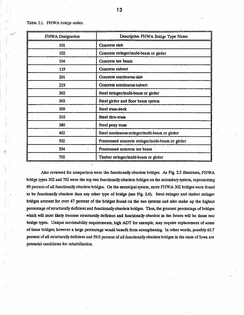
Table 2.1. FHWA bridge codes.
FHWA Designation Descriptive FHWA Bridge Type Name
101 Concrete slab
102 Concrete stringer/multi-beam or girder
104 Concrete tee beam
119 Concrete culvert
201 Concrete continuous slab
219 Concrete continuous culvert
302 Steel stringer/multi-beam or girder
303 Steel girder and floor beam system
309 Steel truss-deck
310 Steel thru-truss
380 Steel pony truss
402 Steel continuous stringer/multi-beam or girder
502 Prestressed concrete stringer/multi-beam or girder
504 Prestressed concrete tee beam
702 Timber stringer/multi-beam or girder
Also reviewed for comparison were the functionally obsolete bridges. As Fig. 2.5 illustrates, FHW A
bridge types 302 and 702 were the top two functionally obsolete bridges on the secondary system, representing
69 percent of all functionally obsolete bridges. On the municipal system, more FHW A 302 bridges were found
to be functionally obsolete than any other type of bridge (see Fig. 2.6). Steel stringer and .timber stringer
bridges account for over 47 percent of the bridges found on the two systems and also make up lhe highest
percentage of structurally deficient a.nd functionally obsolete bridges. Thus, the greatest percentage of bridges
which will most likely become structurally deficient and functionally obsolete in the future will be these two
bridge types. Unique serviceability requirements, high ADT for example, may require replacement of some
of these bridges; however a large percentage·would benefit from strengthening. In.other words, possibly 63.7
percent of all structurally deficient and 59.0 percent of all functionally obsolete bridges in the state of Iowa are
potential candidates for rehabilitation.

({) w ('.) 0 a:: ro
3000
~ 2000 a:: w CD :::;; ::;) z
1000
0
14
34.2%
x>O
8~ 24.8% ~
5<:>0 Lt)~~~ J_JQ~~Ot---------~----------
>< ~ 5<: :> .... ,,. ) <."> ~;o ,,. v
OX
.
4·93 4.73 4.43 4.3% 4. 13 v~,
.c~ 2.2% 1.7% < .e. KXXXI IVVV'I
302 702 402 119 380 502 101 201 504 102 FHWA BRIDGE TYPE
Fig. 2.5. Functionally obsolete county bridges by structure type.

(fl w 0 0 O:'. CD
100
80
~ 60 O:'. w
• CD :::;; :::::> z
40
20
15
/!----·--------·-----·--·-----
302 402 502 201 702 119 101 219 102 380 FHWA BRIDGE TYPE
Fig. 2.6. Functionally obsolete municipal bridges by structure type.

16
With the assistance of the advisory pane~ questionnaires were developed to determine the
strengthening and rehabilitation needs of Iowa's counties and municipalities. Although two questionnaires
were prepared - one for each group - the questionnaires were essentially the same except for some of the
wording; an example of the questionnaire sent to counties may be found in Appendix C.
Each of Iowa's. 99 counties and 77 of Iowa's municipalities, those with populations greater than 5000,
were sent questionnaires. The county response rate was 88 percent; while the municipal response rate was 75
percent.
In the questionnaires, low volume bridges were defined as those bridges with an ADT of 400 or less.
The questionnaires encouraged the inclusion of supplemental information, comments and/or suggestions. Since
responsibilities of the counties are different from those of the municipalities, responses from each were
compiled separately. The questionnaires were divided into two sections. Completion of Section 2 of the
questionnaire was required only if the responding agency had srrengthening or rehabilitation experience.
The purpose of Section 1 of the questionnaire was to determine the Iowa county's/municipality's
experience with bridge strengthening and bridge rehabilitation. The questionnaire defined rehabilitation as
including bridge replacement._ As Fig. 2. 7 indicates o(the counties responding, 43.6 percent had implemented
at least one strengthening method; 81.4 percent had rehabilitated/replaced a bridge.
Fewer municipalities ha~ attempted to strengthen bridges than counties. Of all municipalities
responding, 14.3 percent had strengthened bridges, and 52.6 percent had employed a rehabilitation/replacement J method. It should be noted that 40 percent of all the municipalities either had no bridges, did not have any
bridges with ADT's less than 400, or lacked a situation which could benefit from strengthening. The primary
reason given by counties for not strengthening a bridge was that the deck geometries still would not meet state
width specifications.
Figure 2.8 illustrates those reasons given by the various agencies for not strengthening and/or
rehabilitating/replacing bridges. . The indication is that counties, which are responsible for approximately 16
times as many bridges as municipalities, would benefit more from useful guidelines for bridge strengthening
and replacement. Several respondents indicated that strengthening/rehabilitation had not been used because
of the lack of appropriate expertise.
Questions in Section 2 of the questionnaire were designed to identify the current bridge strengthening
and replacement procedures most often used by county/municipal engineers. Table 2.2 summarizes the
responses to the questions in Section 2 which required a yes/no answer. When asked if any type of economic
analysis was performed in making decisions, respondents noted that decisions were controlled by budget
constraints, structural deficiency priority systems, and the needs of the public, thus making an economic analysis
less effective.
Responses to Question 2 of Section 2 of the questionnaire indicated five counties have developed their
own bridge rehabilitation decision tools which included:

17
~ Counties
~ Municipalities 81.43
w (.'.) .:::: 0.6 1--~~~~~~~~~~~~~~-lQ-QQ<QQ<~~~ z w (.)
. a:: w CL
w U1 z 0 CL f:::] 0.4 a::
0 STRENTHENING R.EHABILITATION/
REPLACEMENT
Fig. 2.7. Experience of local agencies with bridge strengthening and
replacement.

~Counties
~ Municipalities
LACK OF FINANCIAL
RESOURCES
18
LACK OF USEFUL GUIDELINES FOR
DECISION MAKING
LACK OF TRAINED
MANPOWER
Fig. 2.8. Reasons for not implementing strengthening.
i ;

19
• a bridge rating sheet,
• graphs for determining beam spacing,
• tables for determining maximum spacing for various sized timber stringers to meet current legal
load capacities for all wood bridges,
• a simple span bridge rating program used to assist in rehabilitation decisions, and
• charts indicating span lengths and stringer requirements for carrying fully legal loads.
Table 2.2. Summaiy of Section 2 questions.
County Municipalities
Questions Yes No Yes No
1. Do you use formal methodologies (e.g. benefil/cost analysis, equivalent annual cost 21 SS 10 23 method, etc) when making management decisions?
2. Have you developed any design aids, nomographs, software, etc. that are useful in s 13 10 32 making bridge rehabilitation choices?
3. Does ycur agency hire any structural engineering consultants? 68 10 30 3
4. Would your county/municipality benefit from a design aid or decision making tool? 62 9 21 9
S. Are you familiar with the National -Cooperative Highway Research Program Report 20 56 2 31 #293, M!lthods of Streng!!leoin2 Emling Highwa:t Bridges?
A tabulation of the number of counties and municipalities which used the services of structural
engineering consultants is included in Table 2.2; the specific services performed by the consultants are
presented in Table 2.3.
Of those responding to Question 4 of Section 2 (see Table 2.2), county approval was 87 percent and
municipal approval was 70 percent in favor of the development of decision making tools or
rehabilitation/strengthening design aids. Given a list of 'tools' from which the agencies would most likely
benefit, 81 percent of the counties listed computer software development, S2 percent requested nomograpbs;
and 23 percent requested flow charts. Other "tools' counties specified as being beneficial were plans, cost
comparison documentation of rehabilitation versus replacement, a maintenance manual (similar to the one used
in Florida which outlines approved repair practices), and a design manual (similar to the one used in California
which outlines design values and techniques).

20
Of the municipalities responding who favored design 'tools', 67 percent requested computer software,
52 percent requested nomographs, and 52 percent requested flow charts. One municipality noted that design
aids are not necessary since they are a political entity and the insurance liability would be too great; another
municipality noted they will always use a structural engineering consultant for bridge problems.
To determine the strengthening procedures with which counties/municipalities had experience, agencies
were asked to identify procedures they had employed on the four most common structurally deficient types of
bridges. The number of responses by counties were: addition or replacement of timber stringers - SO; addition
or replacement of steel stringers - 31; and lightweight deck replacement in timber stringer bridges - 17.
Table 2.3. Summary of services for which agencies employ consultants.
Consulting Service Counties Municipalities
Structural analysis 61 27
Bridge inspection 52 26
Strengthening or rehabilitation 24 20
New or special bridge designs 11 7
Construction inspection 3 17
Load rating 1 0
Culven design 1 0 .
Underwater inspection 0 1
Municipality responses were: strengthening of existing members on steel pony and through trusses - 6; all
other methods yielded fewer than 3 responses. Responses to the 'other' category were given very infrequently.
Agencies which had employed strengthening methods were asked to indicate which of these methods were
perceived to be ~t effective and structurally effective. Counties noted that the two most cost effective
strengthening methods were increasing transverse stifliless and providing composite action; the two methods
perceived as the most structurally e(fective were the addition or replacement of members and the strengthening
of existing members. Municipalities noted· the most cost effective methods were the addition or replacement
of various members, the strengthening of existing members, and the strengthening of critical connections (equal
number of responses for each.) The two structurally effective strengthening methods noted were the
strengthening of existing members and the strengthening of critical connections. The addition or replacement
of various members was also indicated as being very effective. As expected, those methods which were
perceived as being very costly or structurally ineffective were the methods which have been employed the least.
,1

21
It was suggested that if it were not cost effective to increase the capacity of a given bridge to current
loading standards, a compromise could be reached where the bridge could be strengthened to a specified
increased load. Counties specified in such a case the load they would desire a bridge to carry is 19.1 tons; this
value was obtained by averaging all reported values which ranged between 12 tons and 30 tons. The
municipalities specified 16.4 tons (obtained by averaging reported values) as the desired capacity; reported
values ranged between 10 tons and 20 tons.
The National Cooperative Highway Research Program Report 293, Methods of Stren~hening Existing
Highway Bridges (36), reviews and descnoes currentstrengthening techniques used on existing highway bridges.
Only 26 percent and 6 percent of the counties and municipaliti~, respectively, noted that they were familiar
with this report.
Question 12 on the questionnaire asked the respondents to prioritize the top four deficient bridges into
three categories: 1) the type of bridges which need to be strengthened, 2) those bridges which would most
benefit from a combination of strengthening and posted weight/speed restrictions, and 3) those bridge types
which are least likely to benefit from strengthening or rehabilitation methods. Responses by both counties and
municipalities indicated that steel stringer bridges would benefit the most from either strengthening or a
combination of strengthening and posted weight/speed restrictions.
In summary, a significant percentage of counties are currently employing strengthening methods,
although a limited number of methods are being utilized. Replacement decisions typically tend to be sound
_economical _and structural decisions based on current information available. It appears that part of the
hesitation to strengthen a given bridge is due to lack of adequate information and the bridge's inability to
meet required deck geometries. Both counties and municipalities indicated a rehabllitation/strengthening'tool'
or design aid is desirable. -
The number of bridges per municipality is considerably less than the number of bridges per county.
Apparently the reason municipalities tend not to undertake their own strengthening and replacement designs
is the high cost of liability insurance. However, while counties also employ a large number of consultants, they
are more likely to do some of their own engineering because of the large number of bridges for which they are
responsible and budgetary constraints.
Data from the Iowa NB!, questionnaire responses and input from the advisory panel influenced and
directed the second portion of this investigation (fasks 3-6). Based on information obtained and reviewed in
the initial tasks of this investigation, it was determined that strengthening procedures and techniques which are
applicable to the steel stringer bridges and timber stringer bridges found on low volume roads would be the
most beneficial to practicing engineers. A more detailed summary of the findings of Tasks 1 and 2 are
presented in Ref. 94.
The manual (Chp. 3) thus provides practical strengthening methods for these two types of bridges and
numerous spreadsheets to assist the engineer in designing various strengthening systems.

22
2.4. I.Jlerature Review
2.4.l. Cleneral
A literature search was conducted to gather available information on strengthening/rehabilitation of
low volume bridges. Computeri7.ed literature searches were made using the Highway Research Information
Service through the Iowa DOT and the Engineering Llterature Index System which is available at the university
bbraiy. In addition to searching these two sources, the Geodex System - Structural Information Service was
used to locate additional pertinent references.
The literature search revealed that minimal work bas been done on the general subject of
strengthening, rehabilitating, or replacing low volume bridges. Most of the research which has been reported
has been directed toward one specific type of bridge or set of circumstances.
Literature was located on strengthening/rehabilitating of essentially all types of bridges. However in
this brief literature review, only information on the twO types of bridges previously identified - steel stringer
bridges and timber stringer bridges - as having the greatest potential for being strengthened/rehab~tated will
be presented.
It should be noted at the outset that much of the information related to replacement of low volume
bridges is not located in the published literature, but rather in the form of proprietaiy publications by private
companies. In most cases, these replacement designs are developed on a case-by-case basis. The engineer
submits his site requirements (span length, bridge width, load capacity, and aesthetic considerations) and the
predesigned bridge is shipped to the site essentially complete. These proprietaiy designs will be discussed in
more detail in Chp. 3.
The current AASHTO design s~cations (2) do not distinguish between low volume rural bridges
and high volume urban bridges. Gangarao and Z.elina (28) have suggested that a set of design specifications
and procedures be developed specifically for low volume bridges. They note that it is highly unlikely that
efficient and economical tow-volume bridges can be designed using specifications that were compiled primarily
for highway bridges. Similar thoughts have been expressed by Galambos (27) who suggested specifying rules
for a lower level of serviee for non-Federal aid bridges. Alternatives which allow flexi'bility for site conditions
as well as a proposed fatigue model (both of which would allow Jess structural loading) have been proposed
by Moses ( 48).
In Chp. 1, various FHW A and NCHRP final reports related to bridge strengthening, repair,
rehabilitation, and retrofitting were noted. One of these, NCHRP Report 293 (36) is particularly pertinent to
this study in that it pertains to strengthening highway bridges. This report reviews strengthening techniques
used in the United States as well as in several foreign countries and contains a bibliographywith 379 references
which review the strengthening of all types of bridges. Strengthening information in this report is organized
by strengthening procedure rather than by bridge type as some strengthening procedures are applicable to
several bridge types. Strengthening techniques/procedures in this report were classified into eight categories:
I J
23
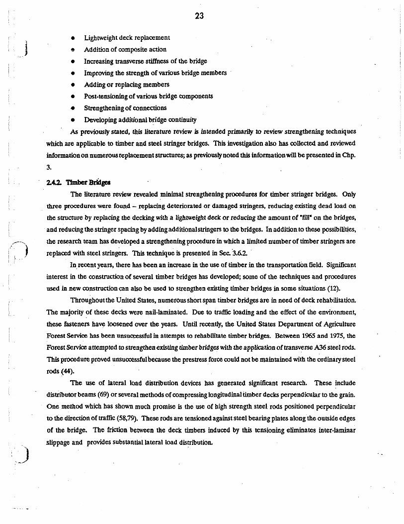
• Lightweight deck replacement
e Addition of composite action
• Increasing tranSVerse stiffness of the bridge
• Improving the strength of various bridge members
• Adding or replacing members
• Post-tensioning of various bridge components
• Strengthening of connections
• Developing additional bridge continuity
As previously stated, this literature review is intended primarily to review strengthening techniques
which are applicable to timber and steel stringer bridges. This investigation also has collected and reviewed
information on numerous replacement structures; as previously noted this information will be presented in Chp.
3.
2.4.2. Timber Bridges The literature review revealed minim•! strengthening procedures for timber stringer bridges. Only
three procedures were found - replacing deteriorated or damaged stringers, reducing existing dead load on
the structure by replacing the decking with a lightweight deck or reducing the amount of 'fill' on the bridges,
and reducing the stringer spacing by adding additional stringers to the bridges. In addition to these possibilities,
the research team has developed a strengthening procedure in which a limited number of timber stringers are
replaced with steel stringers. This technique is presented in Sec. ·3.6.2. ·
In. recent years, there has been an increase in the use of timber in the transportation field. Significant
interest in the construction of several timber bridges has developed; some of the techniques and procedures
used in new construction can also be used to strengthen existing timber bridges in some situations (12).
Throughout the United States, numerous shon span timber bridges are in need of deck rehabilitation.
The majority of these decks were nail-laminated. Due to traffic loading and the effect of the environment,
these fasteners have loosened over the years. Until recently, the United States Depanment of Agriculture
Forest Service has been unsuo:essful in attempts to rehabilitate timber bridges. Between 1965 and 1975, the
Forest Service attempted to strengthen existing timber bridges with tbe application of transverse A36 steel rods.
This procedure proved unsuccessful because the prestress force could not be maintained with the ordinary steel
rods (44).
The use of lateral load distn'bution devices has generated significant research. These include
distnburor beams (69) or several methods of compressing longitudinal timber decks perpendicular to the grain.
One method which has shown much promise is the use of high strength steel rods positioned perpendicular
to the direction of traffic (58,79). These rods are tensioned against steel bearing plates along the outside edges
of the bridge. The friction between the deck timbers induced by this tensioning eliminates inter-laminar
slippage and provides substantial lateral load distnbution.

24
2.4.3. Sleel Bridges
Steel girder bridges, which have a rela.tively small ratio of dead to live load, are especially affected by
an increase in live load. The strengthening techniques found in the literature for steel stringer bridges
essentially all fall in the following six categories:
• Lightweight deck repla.cement.
• Improving the strength of the striiigers.
• Increasing transverse stiffness.
• Adding or repla.cing members.
• Providing composite action.
• Post-tensioning.
The techniques will only briefly be discussed here as there is a very comprehensive literature review of these
strengthening procedures in Ref. 36. To assist tile reader in locating reference material on the various
strengthening procedures, section numbers and page numbers for Ref. 36 have been provided.
Lightweight deck replacement (Ref. 36; Sec. 2.3.1; p 18]: the live-load capacity of a bridge can be
improved by replacing an existing heavyweight deck with a new lightweight deck. A review of the literature
reveals that several structurally adequate lightweightdecks are available, including steel grid, exodermic, timber,
lightweight concrete, aluminum orthotropic plate, and steel orthotropic plates. Each of these will be briefly
discussed in the following paragraphs.
Steel grid deck is a lightweight floor system manufactured by several firms. It consists of fabricated,
steel-grid panels that are field welded or bolted to the bridge superstructure. In application, the steel grids may
be filled with concrete, partially filled with concrete, or left open.
Exodermic deck is a newly developed, prefabricated modular deck system that is being marketed by
major steel-grid-deck manufacturers. The bridge deck system consists of a relatively thin upper layer (3 in.
minimum) of prefabricated concrete jointed to a lower layer of steel gratings.
I aminated timber decks consist of vertically laminated 2-in. (nominal) dimension lumber. The . . .
laminates are bonded together with a structural adhesive to form panels that are approximately 48-in. wide.
The panels are typically oriented transverse to the supporting structure of the bridge and are secured to each
other with steel dowels or stiffener beams to allow for load transfer and to provide continuity between panels.
Structural lightweight concrete can be used to strengthen steel bridges that have normal-weight,
noncomposite concrete decks ( 43). Lightweight concrete (unit weight of 115 lb/cu ft or less) can be either cast
in place or installed in the form of precast panels. Cast-in-place lightweight concrete decks can be made to
act compositely with the stringers.
Aluminum orthotropic deck is structurally strong, lightweight deck weighing between 20 and 25 lb/sq
ft. This proprietary decking system is fabricated from highly corrosion-resistant aluminum alloy plates and
-.,, )

25
extrusions that are shop coated with a durable, skid-resistant, polymer wearing surface. Connections between
the aiuminum orlhotropic deck and the steel stringers should not be consiciered to provide composite action.
Steel orthotropic plate decks are an alternative for lightweight deck replacement, however they are
usually designed on a case-by-case basis with essentially no standardization. Although steel orthotropic deck
is applicable for short spans, it is unlikely that there would be sufficient weight savings to make it economical
Improving the strength of the stringers [Ref. 36; Sec. 2.3.4; p 21 ): One of the most common
procedures used to strengthen existing bridges is the addition of steel cover plates to the existing stringers.
Steel cover plates, angles, or other sections may be attached to the stringers by means of bolts or welds. The
additional steel is normally attached to the flanges of existing sections as a means of increasing the section
modulus, thereby increasing the flexural capacity of the member. When angles are employed to strengthen
stringers, they are usually attached to the webs of the stringers with high strength bolts. In most cases, the
member is jacked up. during the strengthening process, relieving dead-load stresses on the existing stringers.
The resulting cover-plated section will resist both Jive-load and dead-load stresses when the jacks are removed.
If the stringers are not jacked, the added cover plates will carry only Jive-load stresses.
Increasing transverse stiffness of a bridge [Ref. 36; Sec. 2.3.3; p 20): Much of the literature on
transverse stiffness of a bridge deals with the effects of diaphragms and cross frames on transverse stiffness
rather than strengthening of a bridge by increasing the transverse stiffness. Literature indicates that increasing
transvei:se stiffness will be most effective for interior stringers and will have essentially no effect on exterior
stringers. Increasing transverse stiffness should be considered a secondl\ry method of strengthening a bridge.
in most practicai cases, the stress reduction resulting from transverse stiffening is less than 30 percent; in some
cases, it may even be negligible.
Adding or replacing members [Ref. 36; Sec. 2.3.S; p 23): Steel stringer bridges can be strengthened
by the addition or replacement of onp or more stringers. Adding stringers will increase the deck ca pa city and
reduce the magnitude of the loads distnbuted to the existing stringers. This method is most practically
performed in conjunction with replacement of the deck because this allows respacing of the existing stringers.
Stringer replacement is more typically a repair technique that is used when a stringer has been damaged by
an overbeigbt vehicle or corrosion. The addition or replacement of a stringer is more difficult when the existing
deck is not removed. Installation of.the new stringer is usually carried out from below the bridge and is usually
a difficult procedure.
Providing composite action [Ref. 36; Sec. 2.3.2; p 20): Modification of an existing system is a common
method of increasing the flexural strength of a bridge. This procedure can be used when a deteriorated
concrete deck is removed and replaced with a new deck or when the existing deck is sound by coring holes
through the deck, adding shear connectors, and grouting the boles. The composite action of the stringers and
deck not only reduces Jive-load stresses but also reduces deflections as a result of the increase in the moment
of inertia resulting from the stringers and deck acting together.

26
Post-tensioning (Ref. 36; Sec. 2.3.6; p 24]: Prestressing or post-tensioning in various configurations has
been used for more than 30 years to relieve stresses, rontrol displacements and strengthen bridges. Through
research sponsored by the Iowa DOT, Iowa State Universily (ISU) has developed post-tensioning procedures
for strengthening simple-span as well as continuous-span steel-stringer bridges. As has been earlier
documented, the majoriiy of the steel-stringer bridge problems on the low volume roads are with single-span
bridges; thus the strengthening of continuous span bridges will not be discussed in this report.
For the practicing engineer, ISU has developed a post-tensioning strengthening manual (24) that will
assist the engineer in determining the post-tensioningforce a given bridge needs to reduce flexural stresses the
desired amount. In most instances, only .the exterior beams need post-tensioning. Lateral dlstn"bution of the
post-tensioning forces inmost situations also reduces the stresses in the interior stringers.
Several studies have been performed on the cost effectiveness of various bridge strengthening or
rehabilitation methods. In 1985, Cady (13) developed a policy for the decision making process in bridge deck
rehabilitation. An economic mode~ based on the present worth of perpetual service or the capitalized cost
of each alternative was developed. This analysis may be extended to apply to essentially any rehabilitation
project
A study at Pennsylvania State Universiiy (90) developed a flow chart of rehabilitation methods for
highway bridges. A survey of state bridge and maintenance engineers determined the lype and effectiveness
of various maintenance and rehabilitation procedures. These procedures were subjected to a life cycle cost
analysis to determine a range of expected unit costs for the various methods. A now chart was then developed
which would allow a maintenance engi..nC..er to select the most cost effe.ctive rehabilitation method ba..~.d on the
amount of deterioration, ere. This. lype of now chart was found to be very useful to local engineers.
The use of incremental benefit-<X>St analysis has been used by many agencies to aid in the decision
making process. This method identifies the optimum alternatives and also prioritiz.es them. In public projects,
measuring benefits in monetary terms poses a problem. One has to estimate the value of benefits, both for
the agency and for the traveling public from available sources (64).
The use of the benefit-<X>St ratio method to compare possible bridge rehabilitation or replacement
alternatives has traditioully been avoided due to the difficulty in quantifying the benefit of the proposed
improvement. One study which attempted to alleviate this difficully was performed by the New York DOT
Planning Division. To use this procedure, one needs only the posted speed, the average running speed, the
traffic count with some estimate of vehicle mix, and highway section length for both the before and after
conditions (41); with this data, the operating and travel time costs of the alternatives are calculated.
Maintenance and accident costs of the alternatives are not considered in this model
There has been a significant amount of research on the use of value engineering (50) in the design and
constructionoflow volume road bridges. Gangarao, et. aL (29) used value engineering, - that is, th_e systematic
application of recognized techniques which identify the function of a product or service, establish a monetary

27
value for that function, and provide the necessary function reliably at the lowest overall cost - to develop value
graphs, which relate the importance of various b~dge components to their costs.
One major problem with this procedure noted in the literature was the difficulty in predicting the
service life of the various strengthening methods. This obstacle is somewhat mitigated by two factors: 1) as
service life increases, variation in service life has a diminishing effect on calculated equivalent cost and 2) if
the average service lives of relatively short-lived procedures are reasonably well known, rather large variations
will have relatively little effect over the long run.
Engineering economic analyses have historically ignored the effects of inflation. It has been thought
that inflation affects all aspects of cash flow in the same manner, thus its net effect on the decision making
process is negligible. The 1973 oil embargo produced a significant change in the effect of inflation. A marked
reduction in fuel consumption caused a drastic reduction in gasoline tax revenue. At the same time, the cost
of construction increased dramatically due to the rising rate of inflation. Inflation has affected income and
disbursements in opposite directions, creating a situation where engineering economic analysis must take the
effects of inflation into account (14).

MANUAL for EVALUATION, REHABil.ITATION
and STRENGTIIENING OF
WW VOLUME BRIDGES
(Otapter 3)
The contents of this report and the computer programs contained on the provided computer diskette do not represent ~ warranty on behalf ot the State ot Iowa, Iowa State U~ity, or the autho<>. Engineering data, desi&DS> computer progntms and specifications presented in this publication haw: been delineated in accordance with rccognizcd professional principles and prscticcs.
While it is belicw:d to be accurate, this information should not be used or relied •Pon for any specific application without competent professional examination and verification Of its aocuracy, suitability and appJicability by a competent .licensed engineer. Anyone making uac ot this information assumes all liability arising from such use.
.

31
3. APPUCATIONS
As has been previously noted, Chp. 3 of this report is a strengthening manual The other chapters
provide supplementary and background information. Section 3.1. provides general information about the
manual Secs. 3.2 and 3.3 provide basic information about bridge inspection and fundamentals of analysis, I
respectively. Section 3.3 is particulary informative because ten bridge evaluation examples have been provided.
Economic analyses to assist in the decision to strengthen or replace a given bridge is presented in Sec. 3.4.
The remaining three sections of this chapter (3.5 to 3.7) present various strengthening methods and
replacement alternatives.
3.1. General Information
3.1.1. Bactground
As previously noted, the statistical information from the Secondary System Section of the NBI served
as the basis for determining the type of bridges that require strengthening. For additional clarification ofNBI
data, various categories of steel stringer bridges found on the Iowa DOT's county system base inventory record
were reviewed. The program Syncsort was used to sort, extract and summarize information. The year each
bridge was built was reviewed to determine if a correlation existed between the year a particular Iowa DOT
V-series standard bridge was issued and the year a given FHW A 302 bridge was constructed; no clear
correlation was found. Site inspections of several Iowa steel stringer bridges revealed that the majority of these
bridges actually were not construcied in accordance with any of the Iowa DOT V-series.
Lengths and widths of existing FHW A 302 bridges were also reviewed. The average length of the
FHWA 302 bridges found on the Iowa county S)IStem is 50.6 ft. Figure 3.1 illustrates that a majority of the
bridges have lengths between 20 ft and 45 ft. Although, as shown, a number of bridges had lengths over 100
ft, more than likely these bridges are the result of coding errors. As may be seen in Fig. 3.2, the majority of
the bridges have widths of 20 ft and 24 ft. However, a significant number of bridges (over 200 in each case)
have widths of 16 ft and 18 ft.
Two other parameters of interest in the Iowa DOT's county system base inventory record were the
design loading and the design H-loading. The design loading refers to Item 31 in the SI&A data (see Sec. 2.2. );
this one digit code represents the design live load for the structure. Instructions for coding this item require
classifying the loading, if it is other than standard loading, as the nearest equivalentstandard loading. As shown
in Fig. 3.3, in the majority of cases (72.1 percent) the design load is not known; in 20.6 percent of the cases
the design load was classified as H15. Over 93 percent of the bridges fall into these two categories of loading
(HlS or unknown). The design H-loading of the bridge was obtained from maintenance records. The number
of bridges designed for each of the five standard design H-loadings is shown in Fig. 3.4. Note that the design
loading for the majority (71.0 percent) of bridges is unknown (NC).
·As noted in Chp. 2, it was. determined that strengthening techniques are primarily required for
noncornposite, simply supported steel stringer bridges (FHW A 302] and timber stringer bridges [FHWA 702J.

(/) 250 w ('.) 0
gs 200 i.J_
0
8J 150 IIl 2 :::i z: 100 ...J g I- 50
0 15
32
Fig. 3. 1. Lengths of steel stringer bridges: FHWA 302.
1.35

(/) w () 0 Cl'.'. co u... 0 Cl'.'. w co 2 :::::i z ....J g I-
1000
800 -
600 -
400 ....
200 -
0 10
33
V\VVJ. A •f' • I 15 20 25 30 35
BRIDGE WIDTH, feet
Fig. 3.2. Widths of steel stringer bridges: FHWA 302.
' 40 45 50

34
.·~,
'\ ,f
5
72. 13 I") ( 0 4
><
vi w 0 0 3 0:: CD lJ_
0 0:: 2 w CD :l; :J z 20.63 -' ~ 0 I-
4.23 i 1.83 I
0.63 0.43 0.13 0.33 . ......,,
0 NC H10 H15 HS15 H20 HS20 RR MISC
Fig. 3.3. Design load cases: FHWA 302.

35
5
t'}
< 71.0% 0 ~
4 x
(}) w <..'.) 0 3 a:: m L1.. 0 a::: 2 w m 2 21.8% ::::i z _J
;:; 0
4.6% f-1.93 0.33 0.43
0 H10 H15 H20 HS15 HS20 NC
Fig. 3.4. Design H load cases: FHWA 302.

36
Thus, this manual is limited to these two bridge types. One exception to this limitation is the economic analysis
presented in Sec. 3.4; this analysis is applicable to any type of structure.
The economic analysis procedure assists the user in determining if it is more cost effective to replace a
given bridge or to strengthen it. Assuming it is more cost effective to strengthen it, the same analysis procedure
can also be used to determine which strengthening procedures are the most cost effective. The economic
analysis procedure developed makes use of an equivalent uniform annual cost analysis approach and considers
factors such as annual maintenance costs, initial construction costs, service lives, interest rates etc. The various
strengthening techniques and procedures have been organized and presented in this chapter according to bridge
type. Only strengthening and replacement procedures that have been used successfully in the field are included
in this chapter. In the next few years, as a result of extensive bridge strengthening research currently in
progress, and the development of new materials, several new strengthening procedures most likely will be
developed; these could then be easily added to this manual In addition, as databases become available as part
of the development of bridge management systems (BMS), that data will be extremely useful in the economic
model developed in this study.
In the replacement section of this chapter, several proprietary products have been presented. Inclusion
of such products in this manual does not constitute a recommendation by the research team or by the Highway
Division of the Iowa DOT.
3.1.2. Sa>pe of Manual
No special considerations have been accorded skewed bridges. However, the strengthening techniques
presented are applicable to bridges with a small degree of skew.
All strengthening methods presented apply to the superstructure of bridges. No information is included
about the strengthening of existing foundations,since such information is dependent on soil type and condition,
type of foundation, forces involved, etc., and thus is not readily presentable in a manual format. Before
initiating the strengthening of the superstructure of a given bridge, however, one must investigate the
substructure to determine if it is of adequate strength or it also requires strengthening. Some of the
strengthening procedures presented illustrate field welding applications. However, field welding in certain
situations is not the best practice; In older bridges, the type of steel is frequently unknown and thus the
weldability of the steel is also unknown. In these situations, bolted connections should be used unless
laboratory tests are undertaken to determine the steels' weldability. Even when it is determined that the steel
involved is weldable, welding should not be used in locations where it would lower the fatigue resistance of the
original structure. Since the bridges in question have low ADT, fatigue is rarely a problem. However,
strengthening details which may create such problems should obviously be avoided. Potential welding problems
are noted several times in the presentation of the various strengthening techniques.
As previously noted, strengthening procedures are presented by bridge type. In the following sections
the strengthening procedures presented later in this chapter are briefly descnl>ed. Replacement bridge types
are also listed in the following sections and presented in detail later in this chapter

37
Care has been taken to provide the background .for the design procedures for strengthening and
replacement alternatives. Design procedures and calc-.ilations are provided, or references are listed, to provide
appropriate. technical information for a proper analysis and design. The manual user is encouraged to
thoroughly understand the analysis and design application before performing
the final design.
3.1.3. Uso of Manual
The design manual contains information for the bridge engineer ranging from the inspection procedure
to the design of strengthening and/or replacement alternatives. Table 3.1 outlines the major sections of the
manual It is recommended that the user become familiar with the manual's contents prior to using it. The
step by step progression of the evaluation and design process as outlined in this manual includes: (1) bridge
inspection, (2) bridge evaluation (load capacity analysis and, if applicable, desired load capacity goal), (3)
selection of strengthening method and/or replacement bridge type, (4) analysis and design o( items in step 3,
and (5) economic analysis of step 3 alternatives.
Section 3.2 related to bridge inspection is presented to provide important information to perform an
accurate evaluation. Inspection is possibly the most important step in the complete evaluation process and
observations can effect the calculated load capacity of the bridge.
Section 3.3 provides fundamental information for calculating the bridge rating based on inspection data.
The evaluation procedure is outlined and references are provided to assist the engineer in obtaining pertinent
information. Sample calculations are provided to clearly illustrate various evaluation procedures.
Table 3.1. Contents of design manual listed by primary section.
3.2. Inspection
3.3. Fundamentals
3.4. Economic Analysis
3.5. Strengthening Techniques for Steel Stringer Bridges: FHW A 302
3.6. Strengthening Techniques for Timber Stringer Bridges: FHW A 702
3.7. Replacement Bridges
Computer spreadsheets are provided in this manual to perform these evaluation calculations and provide a load
rating, load posting and a maximum SI&A rating.
Once the load rating os the bridge has been determined, a bridge capacity goal must be selected by the
engineer. A strengthening analysis and/or replacement analysis should then be performed once suitable
strengthening methods and bridge replacement types are identified. Sections 3.5 and 3.6 of the manual contain
various applicable strengthening methods for steel stringer and timber stringer bridges, respectively. Based on
the information in this manual, an analysis and design can be performed to achieve the desired bridge capacity
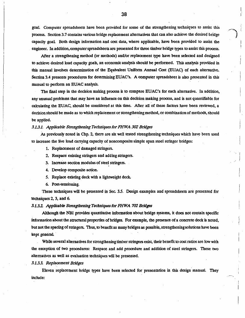
38
goal Computer spreadsheets have been provided for some of the strengthening techniques to assist this
process. Section 3. 7 contains various bridge replacement alternatives that can also achieve the desired bridge
capacity goal Both design information and cost data, where applicable, have been provided to assist the
engineer. In addition, computer spreadsheets are presented for three timber bridge types to assist this process.
After a strengthening method (or methods) and/or replacement type have been selected and designed
to achieve desired load capacity goals, an economic analysis should be performed. This analysis provided in
this manual involves determination of the Equivalent Uniform Annual Cost (EUAq of each alternative.
Section 3.4 presents procedures for determining EUAC's. A computer spreadsheet is also presented in this
manual to perform an EUAC analysis.
The final step in the decision making process is to compare EUAC's for each alternative. In addition,
any unusual problems that may have an influence on this decision making process, and is not quantifiable for
calculating the EUAC, should be considered at this time. After all of these factors have been reviewed, a
decision should be made as to which replacement or strengthening method, or combination of methods, should
be applied.
3.1.3.1. Applica/J/e Strengthening Techniques for 1'1fWA 302 Bridges
As previously noted in Chp. 2, there are six well tested strengthening techniques which have been used
to increase the live toad carrying capacity of noncomposite simple span steel stringer bridges:
1. Replacement of damaged stringers.
2. Respace existing stringers and adding stringers.
3. Increase section modulus of steel stringers.
4. Develop composite action.
5. Replace existing deck with a lightweight deck.
6. Post-tensioning.
These techniques will be presented in Sec. 3.5. Design examples and spreadsheets are presented for
techniques 2, 3, and 6.
3.J.3.2. Applicable StrengtbelliilgTechniquesfor FHWA 702 Bridges
Although the NBI provides quantitative information about bridge systems, it does not contain specific
information about the structural properties of bridges. For example, the presence of a concrete deck is noted,
but not the spacing of stringers. Thus, to benefit as many bridges as possible, strengthening solutions have been
kept general ·
White several alternatives for strengthening timber stringers exist, their benefit to cost ratios are low with
the exception of two procedures: Respace and add procedure and addition of steel stringers. These two
alternatives as well as evaluation techniques will be presented.
3.1.3.3. Replacement Bridges
Eleven replacement bridge types have been selected for presentation in this design manual They
include:
,,_"' I }
I
I

39
1. Precast culvert/bridge.
2. Air formed arch culvert
3. Welded steel truss bridge.
4. Prestressed concrete beam bridge.
5. Inverset bridge system.
6. Precast multiple tee beam bridge.
7. Low water stream crossing.
8. Corrugated metal pipe culvert.
9. Stress laminated timber bridge.
10. Glue-laminated timber beam bridge.
11. Glue-laminated panel deck bridge.
Some of these replacement bridges are proprietaiy. In these cases, general information regarding design
criteria and cost information have been provided. Additional references where more detailed design
procedures already exist have been included for the manual user. Three timber bridge replacement types have
been included. Design examples and spreadsheets are presented for replacement bridge types 9, 10 and 11.
3.1.3.4. Microcomputer Spreadsheets
Responding to the requests of a large percentage of engineers who completed the questionnaires,
computer spreadsheets have been developed for performing various evaluation, strengthening, and replacement
calculations. The primacy advantages of computer spreadsheets for these applications are:
• Most county offices have personal computers which are capable of running spreadsheets.
• Spreadsheet templates can be arranged to follow the normal design process completed by band.
• When changes are made in any part of the input, the corresponding changes in all the calculations are
made automatically.
• Spreadsheet templates can include the necessary tables for beam properties, allowable stresses, etc.
which reduces the calculation time. The software developed in this report is Lotus 1-2·3 release 2.3
(42), which includes the @VLOOKUP function (i.e. Vertical Lookup). This allows easy extraction of
desired values from stored tables.
• Design and revision of spreadsheets is much quicker than conventional programming. Thus, engineers
may take an existing spreadsheet and expand or modify it to better suit their specific needs.
One disadvantage of spreadsheets is that regeneration time increases as the number of equations increases
and the spreadsheet size expands. The number of calculations in the spreadsheets developed in this report are
small so that is not a problem.
Spreadsheets are comprised of labeled rows and columns. Numbers represent rows and columns are
represented by letters. The intersection of a row and column is referred to as a cell; see example spreadsheet
in Fig. 3.5. Cells may include either numerical information, text or commands.

40
STRINGER EVALUATION SPREADSHEET INPUT
~---1-----l'I i-----+--~--rJ
1--=i:==~=---------'----+-----''K
1------lL
1--=ll'"""'"""'""---------L----lM
N
LIVE LOAD + IMPACT MOMENT 0
BRIDGE LOAD IN TON$ P
MAX S.I. & A. RATING 21.AN
Fig. 3.5. Exomple spreadsheet.
20.00 25.00 36.50 40.00 27.25 40.00 40.00

f .; . " '
41
In Fig. 3.5, cells B3 through B8 represent the input for a specific bridge; these cells have been highlighted
in !he spreadsheet Cells B16 through B22 and Cl6 through C22, also highlighted on !he spreadsheet,
represent !he posting values associated with Iowa legal trucks.
A list of the spreadsheets presented in the manual, and their location for various strengthening and
replacement methods and economic analysis is presented in Table 3.2.
Table 3.2. Spreadsheets in design manual
Spreadsheet Application Primary Function Location in Spreadsheet Design Manual Identification (Section No.)
Economic Analysis Analysis 3.4.4 1
Steel Stringer Evaluation Analysis 3.5.2 2
Post-tensioning Strengthening 3.5.6 3
Timber Stringer Evaluation Analysis 3.6.1 4
Stress I aminated Timber Bridge Replacement 3.7.9 s Glue-Laminated Timber Beam Replacement 3.7.10 6 Bridge
Glue-Laminated Panel Deck Bridge Replacement . 3.7.11 7
Prior to an engineer's determination of whether a bridge is a suitable candidate for rehabilitation is the
performance of a thorough inspection of the key elements of the structure. This inspection should be made
by a person wilh at least a general understanding of.how loads arc distnl>uted through a bridge, a knowledge
of what members are ~ain load<arrying elements and what constitutes capacity-reducing damage and
deterioration. ·
Since 1973, bridges have been routinely inspected on a two-year cycle. Therefore, the SI&A reports on
file should indicate which elements of a given bridge warrant closer examination. The information provided
on an SI&A report is not always in a narrative form, but rather is numerically coded with frequently sketchy
comments. A complete report will include structural calculations with a summary of operating, inventory and
posting loads, if they are required.
The most current SI&A report, as well as all previous repons and plans of the bridge in question (if
available), should be reviewed in the office prior to the field inspection. The inspector should have this same
. information available during the actual field inspection.
If the previous inspections have been carefully performed and the data properly and rorrectly reoorded,
the measuring of members and the determination of general dimensions is not necessary each time a given

42
bridge is inspected. However, it is rerommended that the inspector carry a scraper and/or wire brush and
calipers to determine the current sta!US of corrosion and section Joss in the case of steel members.
With the most recent SI&A repon in hand, the inspector shoukl verify the current condition of previously
recorded damage or deterioration. Since this manual deals primarily with simple-span superstructures, it is
assumed that the substructures are sound or can be repaired by practicable, cost-el!ecti'Ye methods pursuant
to repairing and rehabilitating the superstructure.
The principal elements for review are the deck, stringers, bearings, and their ability to interact. The
inspector shoukl keep In mind that the primary purpose of tbis inspection is to view the bridge Crom the aspect
of determining its general condition and suitability for repairs and rehabilitation. That b, can the life of the
bridge be extended for an appreciable (cost-effective) length of time? can the load posting be eliminated or
increased to carry school buses, farm equipmeni, etc.?
3.2.L Deeb
A large number of low volume bridges In Iowa are of timber construction (sec Sec. 2.2), having stringer
elements ranging generally Crom 3 in. x 12 in. to 6 in. x 18 in. spaced for the utilization of 3 in. x 12 in. or 4
in. x 12 in. decking laid transverse to the stringer alignment. Another popular timber deck system is to position
3 in. and 4 in. thick by generally 6 in. to 12 in. wide planks transversely on the stringers on 12 in. to 18 in.
centers and then provide appropriate sized planks longitudinally for what is often called a •deck and a half".
Decks on timber-stringer bridges are usually well spiked to the stringers which, in turn, should have
spacer blocks or X-bracing at bearings and at mid-span to resist transverse •rolling". A timber bridge
constructed in this manner is of little concern regarding the stability of the stringer compression zone.
The method of attaching timber decks to steel str.ngerslbeams is a common area of neglect, which often
leads to the nCed for load posting. :The inspector should review closely the connection between the deck and
stringers. 77le cf«* tar.c•ima • lalietll 6Upp0lt tor Ibo lap llmge ctbeull ud lltrlrl,m and thus must be
appropriately attached.
The allowable stress used by the engineer in computing load capacity is inversely proportional to the
spacing of top-flange points of lateral support; which is provided by adequate-<lepth transverse diaphragms,
deck clips or clamps measured along one side but staggered back and forth along both sides of the flange,
power-driven fasteners, etc. In some instances, a bridge can have its posting removed or significantly reduced
very simply and economically by reducing the spacing between points of lateral suppon on the top flange.
The load capacity is also inversely proportional to the width of the compression flange of the stringer
or beam. It is imponant that the inspector determines the current area and configuration of top-flange as well
as general corrosion and section loss. Top flanges of stringers supponing timber decks are naturally subject
to section loss due to deck leakage. As a general concern, the inspector should determine whether the existing
condition (decay, insect infestation, dry roi, etc.) of the timber will allow it to act as a sound structural element
and whether it can support the fasteners previously descnoed which provide lateral suppon to the compression
flange of the steel stringers/beams.
' I !

43
Timber decks often have rock or earth fill ranging from light to very substantial This naturally reduces
the live load capacity of the bridge and inlu1>its determination of the condition of the deck. Before a
rehabilitation scheme is developed for a given bridge, consideration should be given to adjusting the gradeline
which could remove or reduce the deck fill, which in tum would influence the method of rehabilitation and/or
strengthening.
The rehabilitation of concrete decks can often be accomplished using a high-density concrete or latex
modified concrete overlay. Such overlays usually prolong the life of the deck for a substantial period of time,
but also reduce the live load capacity of the bridge. For bridges that are marginally 'legal' this extra weight
may require the bridge to be posted if provisions were not made for a 'future wearing surface• in the original
design. Whether a concrete deck is removed and replaced as pan of the overall rehabilitation of the bridge
will influence the approach taken to improve the load capacity of the stringers. For example, if the deck is
removed from a steel stringer bridge which has no composite action between the deck and the stringers, the
load capacity of the bridge can be easily and economically improved by designing and installing shear studs to
the stringers for composite action before replacing the decks and/or respacing and adding stringers. The
emphasis here is that the inspector s.hould provide enough detailed data (surface spans, map cracks,
delamination, rebar exposures, etc.) regarding the deck condition to determine if it is cost effective to salvage
the deck, rf?pair it by patching, overlay it, or remove it to facilitate a more practical method of strengthening
the stringers.
Full-depth deck cracks can often be detected by the presence of effiorescence on the bottom of the deck
and by rust on the edges of the top stringer flanges. If plans are not available indicating the presence of shear
connectors for composite actions, coring of the deck over the stringers should be considered to determine if
shear connectors are present.
Another situation for overall strengthening is that in which it is determined that the non<0mposite
concrete deck needs replacing and the stringers are slightly sub-legaL If the concrete deck is removed and
replaced with a properly designed and installed timber deck, the reduction in dead load and the resulting
increase in live load capacity could be substantial Naturally, existing stringer spacing and the economy of
respacing is imponant here. A concrete deck can provide lateral suppon for the compression flange of steel
stringers if that flange is embedded. in the bottom of the deck.
The use of metal decks is not too common, but their inspection should include the spacing and quality
of fasteners (usually welds) which attach the deck to the stringers. Most metal decks are a commercially
designed product. The manufacturer's specifications, unit weights and recommended installation methods
should be obtained and reviewed. The inspector should also be concerned about the presence of cracks in the
ponland cement or asphaltlc concrete topping reflecting from the corrugations in the metal pans. This is quite
common and leads to moisture reaching and corroding the metal decks.
Metal decks - as an element considered for strengthening and rehabilitation - can offer a durable,
relatively light-weight deck and may have, in some situations, advantages relative to reinforced concrete or

44
timber. The closely spaced welds usually specified provide good lateral support of the steel stringer ,,~""
compression flange. }
As a final emphasis, inspection and evaluation of decks should consider not only their condition and load
can:ying capacity as an isolated structural element, but aiso the effect the deck has, or could have, on the
stringer system in terms of lateral support, composite action and reduction of dead load.
3.2.2. Strlngeil/Bcama
Inspectors should recognize signs of distress in stringer systems. In timber bridges, the top fibers of the
stringers are subject to high moisture content and rot caused by deck leakage. The inspector should probe this
area and other suspicious areas, such as around bearings, with an ice pick to determine the reduction in useful
section. It is a practice in some places to deal with top fiber rot by removing the deck and turning the stringers
over. This provides better material for re-spiking the deck to the stringers, but doesn't improve the stringer
-apacity because it still has the same effective depth and now the decayed fibers are in tension. The area
. around knots, especially in the middle-third of the span near the bottom tension fibers, should be inspected
closely for signs of horizontal splits or fiber failure.
Horizontal splits is a serious form of failure, although some residual capacity remains. For example, a
4 in. x 16 in. stringer with a hotjzontal split at ntid-depth yields two 4 in. x 8 in. pieces. The resulting section
modulus is then 2(4 x S1/6) == 85.3 in' which is half of that of the uruiplit 4 in. x 16 in. which is (4 x 16'/6) =
170. 7 in3• The prese!lce of .short horizontal splits at the stringer ends effects shear capacity.
The inspector should be alert for excessive twist (out-of-plane bending), sweep (horizontal deflection)
and vertical deflection (usually caused by under design or excessive fill on deck). Twist, sweep and the sudden
lateral 'rolling' of the stringer system (domino effect) can be effectively controlled by the use of spacer blocks
or sturdy x-bracing at the bearings and at mid-span.
Insects, usually termites or carpenter ants, can be very destructive. Often a stringer will appear normal
in size and surface texture, but will have its interior fibers eaten away. Tapping and probing of the surfaces
and observation of the sawt:d cross-section at the stringer ends should be a routine part of any timber bridge
inspection.
The rehabilitation and strengthening of timber stringer bridges (see Sec. 3.6) is routinely accomplished
in several ways, such as by simply substituting sound members for individual damaged or undersi7.ed members,
by dismantling and re-erecting with sound members of the same or larger size, by using a mix of sound. and
salvageable members either at the same stringer spacing or at a smaller spacing, determined by calculation,
or by inserting sound members into the spacing between existing stringers, which arbitrarily cuts the spacing
in half. In any case, the spacer blocks or X-bracing will have to be removed, modified and reinstalled.
Naturally, calculations should be prepared to provide comparison data on cost, practicability, and benefits
gained by eliminating or reducing the load posting requirement.
Again, the inspector should keep in mind that the data to be gathered are to be used in the rehabilitation
and/or strengthening of the bridge in question, not merely to determine its present condition and load capacity.

45
Any observations or suggestions thought to be helpful should be recorded.
The inspection of steel beams or girders should take the same general approach as with timber. Instead
of decaying timber, !here is corroding metal Instead of timber decks which don't interact with timber
stringers to produce a greater load capacity, !here may be concrete decks which may be composite with the
beams or girders through the use of shear connectors.
Whereas decaying timber is irreversible, !he life of a steel member can be extended by thorough cleaning
and painting. The inspector should note, measure and photograph heavily corroded areas. The extend and
location of corrosion will influence a decision on whether to incorporate the damaged member into !he
rehabilitation plan by determining, with calculations, whether the' loss of section will reduce the load capacity.
The inspector will often find !hat a steel stringer bridge with a timber deck will have that deck affixed
to the top {compression) stringer flange with clips located only along one edge of the flange. This practice
offers no restraint to lateral movement in the direction opposite the clips. If the member was properly
analyzed for this condition and it was determined to govern the load posting, strengthening can be achieved
by removing the deck and resetting it wilh clips placed alternately along each side of the flange. If the required
equipment is available, the same results can be achieved with power-driven fasteners, usually spaced at about
2 ft on centers.
The inspector should verify !he size ~nd location of bolt holes often found in webs and tlanges of re
erected beams and stringers taken from stockpiles of dismantled bridges. The size and location of any bottom
tlange cover plates should also be noted. Strenglheningmay be achieved by attaching cover plates if none exist
or additional plates if practicable, to the existing beams.
As with timber, the inspector should note any twists, sweep or excessive vertical deflection. Fatigue
cracks are not too common in simple-span bridges on low-volume roads, however, they may result from out-of·
plane bending, base metal 'notching' caused by careless welding, a poorly designed structural attachment, etc.
Therefore, beam and girder webs should be carefully examined at the top and bottom of diaphragm or floor
beam connections; flanges at the ends of cover plates should also be carefully examined. Fatigue cracking can
usually be arrested if detected in the early stages.
Leaf rust, !hat is the lamination of metal in !he corrosion process, is often found near the ends of beams
at leaking expansion joints and at .the interface of pieces such as angle lel}' and webs of built-up girders,
diaphragm-to-stiffener connections, or under cover plates or gusset plates.
The location and severity of fatigue cracks and corrosion and the practicability of making repairs must,
of course, be included in the rehabilitation decision process to minimize the possibility of 'putting good money
after bad'.
3.2.3. DiaJna, Bcaringll and Expansion Joinlll
Leaking decks, floor drains that do not extend below the bottom of the bottom flange of the beams or
girders and expansion joints that teak, such as the once common plate-on-plate device, are sources of
concentrated corrosion-producing drainage. The inspector should note any observations in this regard so that

46
necessary changes (such as extending or plugging floor drains, replacing leaking expansion joints with neoprene .. '\
gland or closed-cell joillts, etc.) cm be included in the rehabilitation plan. Where a new concrete deck is i planned, expansion joints and deteriorating abutment backwalls can be eliminated by pouring an abutment
diaphragm integral with the slab and flush against the cap or footing bridge seat using doweled-in reinforcing.
The inspector should note the condition or repairability of the cap or footing.
Bearing material in steel bridges is very vulnerable to corrosion caused by drainage through timber decks
or the aforementioned leaking expansion devices. This drainage often ponds on the bridge seat and inundates
the masonry plates. Over time, the corrosion will cause the bearing plates to •freeze-up•. The immobility of
joints and bearings is alsO often caused by movement of the abutments toward each other causing the backwalls
to jam against the ends of the beams or girders. The bridge, expanding in the summer months, but having
•frozen• bearings, could impart forces of damaging magnitude.
The inspector should note if the expansion device is closed, the severity of rocker tipping, the dis19:nce
between the beam ends and front ~ce of backwall, etc. These problems may require some rehabilitation of
the substructures to allow the superstructure to be more functional and unrestricted by secondary loads and
forces.
7"omugb l1J8p«tioa ii impottalltl Plans for rehabilitation and strengthening should not proceed until
the data gathered has been reviewed and a feasibility study, including preliminary pricing, bridge life, and load
capacity benefits has been prepared. Good inspection and reporting may expose problems of such a magnitude
that rehabilitation and/or strengthening are not cost effective.
Pursuant to preparing a load capacity analysis for a simple-span steel beam or timber stringer bridge is
the assembly of dimensional, material, loading and condition data.
If plans (preferably as-built) are not available, field measurements will be required to determine:
• Beam/stringer si7.Cs
• Beam/stringer lateral spacing
• Center to center of bearings
• Type, size and spacing of diaphragms (steel) or blocking (timber)
• Width, thickness and type of deck
• Depth and type of any wearing surface present (concrete or asphalt overlay, rock or dirt fill)
3.3.2. Matmfals (Allowable SU-)
3.3.2.1. Steel
Plans prepared within appro:timately the past twenty-five years will show material strengths (allowable
stresses). If this information is not available on the plans, but the year of construction is known, the yield

47
strength (F,) for steel componenrs can be assumed as follows:
• . Prior to 1905 26,000 psi
• 1905 to 1936
• 1936 to 1963
• 1963 to Present
30,000 psi
33,000 psi
36,000 psi
If neither material strength or year of construction is available, the engineer is left to his/her best
judgment; one shouldn't, however, assume· a yield strength greater than 30,000 psi. The AASHTO manuals
(2) includes a table of allowable streSSes for steel in Sec. 10; allowable steel stresses may also be found in Sec.
5 of Ref. 3.
The allowable stress to be used in analysis is O.SS F1 for the 'Inventory" capacity and 0.75 F, for the
•Operating' capacity, except as modified when the compression· flange is not fully restrained against lateral
movement. In these cases, the following is used:
Allowable inventory stress, f,,. = O.SS Fy • K(Llb)
where:
F1 = appropriate yield strength as determine above
K = 3.9 for F1 = 26,000 psi
5.2 for F1 = 30,000 psi
6.3 for F1 = 33,000 psi
7.S for F1 = 36,000 psi
L = spacing (in inches)of feature that restrains the compression flange
from lateral deflection in both directions, (e.g. diaphragms, power
driven fasteners, clips, etc.)
b = width (in inches) of compression flange
Ub shall not be greater than 42, 39, 38 and 36 for the respective F, values listed in the definition of 'K'. If
these limits are exceeded, 'L' should be reduced by some physical alteration. The allowable operating stress
for a partially restrained compression flange is the inventory stress r, as calculated above, times a factor of 1.37.
3.3.2.2. Timber
The determination of allowable stress in timber stringers and decks begins with knowing the species and
grade of lumber used in the member to be analyzed. The appropriate allowable value (shear, bending! tension,
compression, etc.) can then be obtained from tables in Section 13 of the 'Standard Specifications for Highway
Bridges' (2) based on member size and usage with subjective reductions based on the engineer's judgment,
considering whether the timber is treated. or untreated, its moisture content, age, condition, etc. This stress
may be considered as the allowable 'Inventory" stress. The allowable 'Operating' stress should not exceed 1.33
times the allowable 'Inventory" stress.

48
3.33. LoadS
• Dead Load
Decks -
Timber = so lb/cu.ft
Concrete = lSO lb/cu.ft
Steel = 490 lb/cu.ft
Wearing Surface - .
Concrete = lSO lb/cu.ft
Asphalt = 144 lb/cu.ft
Rock = 120 lb/cu.ft
Dirt ·= 125 lb/cu.ft
Rails -
As determined by measurement and the above unit loads or from tables.
Curbs-
Based on measurements and type of material.
Beams/Stringers -
If plans or shop drawings are not available, steel beam weights can be read from tables
in the American IDstitute of Steel Construction Manual (AISC) (6) once the beam
dimension$ are carefully determined. Timber stringer weights are based on field
measurements and SO lb/cuft.
Diaphragms or Blocking -
Load per foot of beam/stringer is the weight of one diaphragm or blocking unit divided
by the longitudinal spacing of the diaphragms or blocking.
Other Attachments -
Pipes, conduits, cattle restraints, etc (as determined by the engineer)
• Lfye Load
The FHW A requires that the "Operating Rating" and "Inventory Rating" be based on "HS" (AASHTO
Loading) a5 graphically defined in Fig. 3.6. Any analysis involved in rehabilitation and strengthening to
determine posting requirements for Iowa legal trucks should include the "HS" capacities as welt
Figure 3.7 shows the axle loads and spacing for the Iowa legal trucks. Bending moments in ft-kips per
wheel line for these vehicles are presented in Appendix B. A wheel line is defined as the wheels on one side
of the truck.
The bending moments determined from the tables in Appendix B must be distnbuted laterally to
establish a per beam/stringer bending lriomenL This distnbution is determined from Article 3.23 AASHTO
(2). "One Traffic Lane• distnbution is to be used when the roadway width is 18 ft or less and "Two Traffic

8.0 k
i I· ;::! "l I o;
i o: 1W
I i i i i I
0.1W
49
32.0 k * 32.0 k *
~ i 14'-0"
~1-v
·! HS 20-44
~! ~i ol ol
j i 1--·-l[~o~A~:w,,_-._t------~-
! i
. i
~---~----·--. ·-1 0.4W
i
W = Combined weight ·an the first two axles which is the ·same as for the corresponding H (M) truck.
V = Variable spacing - 14 feet to 30 feet inclusive. Spacing to be used is that which produces maximum stresses.
Clearance and load lone width
10'
Wheel Loads
... 12·1 .. 5' •1 2'1• Standard HS Trucks
Curb
* In the design of timber floors and orthotropic steel decks ( exluding transverse beams) for HS 20 loading: one axle load of 24,000 pounds or two axle loads of 16,000 pounds each, spaced 4 feet apart may be used, whichever produces the greater stress, instead of the 32,000-pound axle shown.
Fig. 3.6. AASHTO standard loads.

50
RATING VEHICLES (Showing axle loads in kips.)
12k
} 11 '
l
14.5k
l 15'
l ~
1.
11'
19· I TYPE 4
weight = 54.5 kips
13k 13k
f 41f 20'
43'
TYPE 353 weight = 80 kips
12k 12k 13.5k i 4'±· 1 O' i
43'
TYPE 3-3 weight = 80 kips
Fig. 3. 7. Iowa legal loads.
14k 14k 14k
·f 4'±·4'{
. . I
14 k 14k 10' ·i 4
'·1 . l
\ l /

51
Lanes• distnbution is to be used for bridges with roadways greater than 18 ft. County bridges with roadway
widths .requiring analysis for more than two lanes (36 ft) are rare and will not be considered here.
Live toad distnbution for timber decks is addressed in Articles 3.25 and 3.30 of AASIITO (2) and will
be demonstrated in example calculations which follow.
• Impact
Impact is included in the total toad determination as a fraction of the calculated live load. As noted in
Article 3.8.1 of AASIITO (2), impact is not to be considered for timber structures.
The impact fraction is determined by the formula:
50 I= < 0.30 L+125 -
where: I = impact fraction (maximum 0.30)
L = span length, center to center of bearings for simple span bridges in ft.
Dimensions of stress-carrying members can change over time due to corrosion, decay, wear (decks),
damage from external forces (ice and drift flows), etc. This naturally causes a reduction in member cross
section resulting in a smaller section modulus, S. The bending stress, f., in a member is equal to the bending
moment M divided by the section modulus, thus: .
M 1~ = -s
Therefore, the bending stress, f., is inversely proportionalto the section modulus S. It is not uncommon
to find bolt holes in the webs and flanges of steel beams, usually when a member has been re.erected from
stockpiled material The section modulus should be calculated to reflect the presence of these holes. It is
important during the gathering of dimensional data that the location of any localized reduction in section be
identified along the beam span relative to the centerline of bearing so that the reduced bending moment at
that location can be computed.
A uniform toss of section due to light overall rusting of a steel member can be estimated by the
inspector. The section modulus may be reduced 1 to 5 percent When heavy rust and P!tting are present, the
beam should be spot-cleaned with a wire brush and measurements taken with a caliper and metal tape.
Loss of section in timber stringers is also based on judgement and measurements taken by probing a
member with an ice pick or a similar instrument A reduction in allowable stress as well as in section should
be considered by the engineer. The expression for the section modulus of a timber stringer is:

where,
52
bd S=-6
b = effective width of member.
d = effective depth of member.
County simple span steel beam bridges, with very rare exceptions in Iowa, can be placed in Case III of
Table 10.3.2A of AASHTO (2). In other words, the bridge being considered will not likely be located on
'Freeways, Expressways, Major Highways, and Streets• having high average daily truck traffic (AD1) ..
Therefore, the reduction in allowable stresses due to fatigue caused by large stress ranges and high cyclic
loading will not govern and will not be discussed here, other than to say that poor quality and poorly designed
welds indiscriminately located can be a source of member failure. Therefore, all welding employed in
performing repairs and strengthening procedures should be approved by the engineer and performed by a
certified welder in strict adherence to current and applicable codes of the American Welding Society including
such considerations as weldability of base metal, selection of proper welding rod and power setting, welder's
position (i.e. overhead, vertical, down-hand, horiwntal), weather conditions, etc.
3.3.S. Ra1fng
The following ten numerical examples assemble the above data and information into operating and
inventory ratings and load posting by means of the following steps:
1. ca!culate.allowable bending stress (F,) in beam or stringer based on information
descn"bed in Materials (Allowable Stresses) (Sec. 3.3.2).
2. Calculate actual dead load bending stress (f.t) in beam or stringer using a
uniform load per foot of span (w) as descn"bed in "Loads" (Sec. 3.3.3) and applying
the following formulas:
M (Dead Load Moment) = w x V/8
where,
L =span
f.t =MIS
where, S is the section modulus as descnbed in Condition (Sec. 3.3.4).
3. Record the gross weight of the applied truck in tons for which rating or posting
is being calculated:
HS20 = 36 Tons
Type3
Type4
= 25 Tons (Governs for Deck Analysis)
= 27.25 Tons

Type 3S3 = 40 Tons
Type ~-3 = 40 Tons
53
4. Calculate actual live load bending stress in beam or stringer (including impact except for timber
members) using moments from tables in Appendix B which are based on truck dimensions and axle
loads shown in Figs. 3.6 and 3.7. These tabular moments, given in ft-kips, should be convened«>
in.-lbs by multiplying by 12,000 (12 in./ft x 1,000 lb/kip). This moment should then be multiplied
by a factor for lateral distribution. The resulting stress when this moment is divided by the section
modulus will be designated as (~).
where,
T = F, = r.. = t; =
The rating of the member can now be calculated by the expression:
rating vehicle in tons
R.ating (Tons) = (F • - f) T ft
allowable bending stress
dead load bending stress
live load bending stress
The following examples are included to illustrate the above method. For clarity, larger type size bas
been used for the examples.

54
3.3.6. Examples
3.3.6.1. Example 1: Timber stringers (1 ft-6 in. on center); Timber deck with rock fi71
GIVEN: 4 in. x 16 in. Timber Stringers @ 1 ft-6 in. c to c Span = 24 ft One Lane Bridge (W ~ 18 ft) 3 in. x 12 in. Transverse Plank Deck Full Lateral Support 4 in. Rock Fill (120 lb/cf) Fb INV= 1600 psi. FbOPER= 1600 psi(l.33) = 2128 psi
DEAD LOADS:
Deck: ( 3 in )(so ~) c1.so ft) 12 in/ft ft
Stringer: f 4 l/8inl (16 l/2in~ (50 lb) (nominal dimensio ~) 144 in2/ft2 ft:S
Rock: ( 4 in )(120 lb) (l.50 ft) 12 in/ft ft3
= 18.75 lb/ft
= 20.86 lb/ft
= 60.00 lb/ft
Misc: = 2.39 lb/ft WDL = 102.00 lb/ft
Mol = ~ = 102 lb/ft (24 ftl 2 = 7344 ft-lb 8 8 .
Section Modulus, Sb= 1/6(4 l/8in)(l6 1/2in) 2
Sb= 155.16 in3
fbDL = ~l = 7344 ft-lb (12 in/ft} Sb 155 .16 in3
= 567.8 psi
LIVE LOADS:
Impact: I = o (For Timber Structures)
Wheel Factor: (AASHTO TABLE 3.23.l: Timber Plank Floor: Timber Longitudinal Beams; Bridge Designed For One Traffic Lane)
W.F. = __§_ S = Stringer Spacing 4.0
W.F. = 1.5 = 0.375 4.0

55
Live Leads, continued:
Mm ox
l\L = (Moment Due To Live Lead Truck) x (l+Impact) x (Wheel Factor)
P,
x
L Maximum moment due to truck loads on a simple span can be determined by use of a general rule. The maximum bending moment occurs under one of the wheel loads when that wheel load is as far from one support as the center of gravity of all the wheel loads is from the other support. The relationship is shown to the left.
The relationship was used to determine the maximum live load moments for different truck types on different lengths of spans (see Appendix B. )
l\L (HS20) = (96.00 ft-kips) (1.0) (0.375) (1000 lb/k) == 36,000 ft-lb
l\L<TYPE4) = (98.00 ft-kips)(l.0)(0.375)(1000 lb/k) = 36,750 ft-lb
l\L (TYPE 353)= (98.00 ft-kips) (1.0) (0.375) (1000 lb/k) = 36, 750 ft-lb
l\L<TYPE3·3)= (77.53 ft-kips)(l.0)(0.375.)(1000 lb/k) ='0 29,074 ft-lb
fblL = Mi_L s;
fbl.L (HS20) = 36,000 ft-lb (12 in£'.ftl = 2784.22 psi 155.16 in3
fbl.L (TYPE 4) = ;}6,750 ft-lb (12 inlft) = 2842.23 psi 155.16 in3
f bl.L <TYPE 353) = 36,:Z50 ft-lb 155.16
(12 in3 inlftl = 2842.23 psi
fbl.L <TYPE 3-3) = 29,Q74 ft-lb £12 inlft} = 2248.57 psi 155.16 in3

HS20 RATING:
HS Rating =
Inventory = Rating
Operating = Rating
LOAD POSTINGS:
Rating/ = Posting
w =
Type 4 =
Type 4 =
Type 3S3 =
Type 3S3 =
Type 3-3 =
Type 3-3 =
56
~All~abl•} (Dead !Dad~ Stress - Stress (36T) Live Load stress
(1600 12si - 567.98 J2si) (36T) = 2748.22 psi
~128 12si - 56Z.98 12si) (36T) = 2784.22 psi
~Operating ( Oead Loa~ ·Stress Stress (W) Live Load stess
weight of truck causing the live load.
(2128 12si - 567.98 12si) (27.25T)
2842.23 psi
14.96 T - Post for 15 Tons
(2128 J2Si - 567:98 psi J (40 T) 2842 .. 23 nc,
\ ,,.-- - I
21.96 T - Post for 22 Tons
(2168 12si - 567,28 12si) (40 T) 2248.57 psi
27.75 T - Post ;fo:i,: 68 :t:ons
,.-.._,,, ¥
13.3 tons
20.2 tons

57
3.3.6.2. Example 2: Timber Stringer (1 ft-6 in. on center); Timber Deck
GIVEN:
Same as Example 1, without rock fill.
DEAD LOAQS:
Deck: (. 3 in \(so ~) (1.so ft) = 18.75 lb/ft \12 in/ft} ft
Stringer: fj4 l/8inl (16 l/2in)~ ( 50 lb) "" (nominal dimensions) 144 in2/ft2 ft~
L
20.86 lb/ft
Misc:
Mot = wlZ = 8
LIVE LOAQS:
= 2.39 lb/ft WDL = 42 • 00 lb/ft
42 lb/ft {24 ftl 2 = 8
3024 ft-lb
3024 ft-lb (12 in/ft\ 155.16 in3
= 233.88 psi
Live Load Moments (~L) and Live Load Stresses (f~L) are the same as those calculated for Example 1.
HS20 RATJ;N~:
HS Rating = ~All~able) (Dead Load~
(36T) Stress - Stress Live Load Stress
Inventory = (1600' IlSi - 233. 88 IlSi) (36T) = 17.7 tons Rating 2784.22 psi · ·
Operating = (2128 12si - 233.88 IlSi) (36T) = 24.5 tons Rating 2784.22 psi

LOAD POSTINGS:
Rating/ Posting
Type 4
Type 4
Type 3S3
Type 3S3
Type 3-3
Type 3-3
58
Live Load
. ( Dead Load~ Stress (W) = ~{Operating) Stress -
Stess
W = weight of truck causing the live load.
= (2128 psi - 233. 88 psi) (27. 25T) \ 2842. 23 ps;
= 18.16 T - Post for 18 Tons
= (2128 psi - 233.88 psi) (40 T) 2842.23 psi
= 26.66 T - Post for 27 Tons
= (2128 psi - 233.88 psi) (40 T) 2248.57 psi
= 33.70 T - Post for 34 Tons

59
3.3.5.3. Example 3: Timber Stringers (1 ft-2 in. on center); Timber deck with rock ff17
GIVEN:
Same as Example l with l ft-2 in. stringer spacing.
DEAD LOADS:
Deck: ( 3 in )(so lb) (l.167 ft) = l4.S8 lb/ft 12 in/ft ft3
= stringer: [c3 7 /8 in> ClS 1/2 inj (so lb) (nominal dimensioE') 144 in2/ft2 ft3
20.86 lb/ft
Rock: ( 4 in ) (120 ~) (l.167 ft) = 46.67 lb/ft 12 in/ft ft
Misc: = 2.89 lb/ft WDL = 8S • 00 lb/ft
MnL = wl2 = 8S lb,::'.ft {24 ft) 2 = 6120 ft-lb 8 8
ftol =Hot = 6120 ft-lb c12 inLftl = 473.32 psi Sb 1S5.16 in3
LIVE LOADS:
Impact: I = o (For Timber Structures)
Wheel Factor: (AASHTO TABLE.3.23.1; Timber Plank Floor; Timber Longitudinal Beams; Bridge Designed For One Traffic Lane).
W.F. = _§_ S = Stringer Spacing 4.0
W.F. = 1.16 = 0.292 4.0

HS20
60
1\L = (Moment Due To Live Load Truck) x ( l +Impact) x
1\L (HS20) = (96.00 ft-kips) (1.0) (0.292) (1000 lb/k)
1\L(TYPE 4) = (98.00 ft-kips)(l.0)(0.292)(1000 lb/k)
1\L (TYPE 353)= (98.00 ft-kips) (1.0) (0.292) (1000 lb/k)
1\L (TYPE 3·3)= (77.53 ft-kips) (1.0) (0.292) (1000 lb/k)
fbll = Hi.l s;
fbll (HSZO> = 28,032 ft-lb (12 inLft} = 2167.98 155.16 in3
fbll (TYPE 4) = 28,6:!.6 ft-lb (12 inLftl = 2213.15 155.16 in3
fbll (TYPE 3S3) = 28,6:!.6 ft-lb (12.inLftl = 2213.15 155.16 in3
fbll (TYPE 3·3) = 22,639 ft-lb (12 inLf:tl = 1750.89 155.16 in3
RATING:
HS Rating = ~All~abl•) (Dead !Dad~ (36T) S:!;ress - Stress Live Load Stress
Inventory = (1600 :esi - 473.32 ;esi)(36T) = Rating 2167.98 psi
Operating = (2128 ;esi - 473.32 ;esi) (36T) = Rating 2167.98 psi
(Wheel Factor\ ' i
= 28,032 ft-lb
= 28,616 ft-lb
= 28,616 ft-lb
= 22,639 ft-lb
psi
psi
psi
psi
18.7 tons
27.5 tons

LOAD POSTINGS:
Rating/ = Posting
61
~operating) · 1
(Dead Loa~ Stress - Stress (W)
Live Load Stess
w = weight of truck causing t.he live load.
Type 4 =
Type 4 =
Type 3S3 =
Type 3S3 =
Type 3-3 =
Type 3-3 =
(2128 psi - 473.32 psi) (27.25T)
2213.15 psi
20.37 T - Post for 20 Tons
(2128 psi - 473.32 psi) (40 T) \ 2213.15 psi
29.91 T - Post for 30 Tons
(2128 psi - 473.32 psi) (40 T)
. 1750.89 psi ·
37. 80 T - Post for 38 Tons ·

62
3.3.6.4. Example 4: Steel stringers with full lateral support of compression flange
GIVEN: 18 x 54.7 Al!lerican Standard I-Beam @ 3 ft - 4 in. spacing c to c Span = 40 ft Two Lane Bridge (W~l8 ft) 4 in. x 12 in. Transverse Plank Deck Full Lateral Support of Compression Flange 2 in. Rock Fill (120 lb/cf) FY= 33,000 psi (1936 to 1963)
DEAD LOADS:
Deck: ( 4 in )(so ~)(3.33 ft) = 12 in/ft ft
Stringer: =
Rock: ( 2 in ) (120 lb ) ( 3 • 3 3 ft) = 12 in/ft ft3
Misc: = WDL =
55.56
54.70
66.67
5.07 182.00
1\L = wl2 = 182 lbLft (40 ft} 2 = 36,400 ft-lb s 8
lb/ft
lb/ft
lb/ft
lbLft lb/ft
Sb = 89.4 in3 (AISC Design Manual)
fbDL = MoL = 36400 ft-lb (12 inLftl = 4885.91 psi Sb 89.4 in3
LIVE LOADS:
Impact: I = 50 :5. .30 (AASHTO 3.8.3.1) L + 125
I = 50 = 0.303 > 0.3 40 + 125
I = 0.3
i i

63
Wheel Factor: (AASHTO TABLE 3.23.l; Ti:mber Plank Floor; Bridge Designed For Two Traffic Lanes)
W.F. = _S_ 3.75
S = Stringer Spacing
w.F. = 3 ft -4 in = o.889 3.75
1\L = (Moment Due To Live Load Truck) x (l+Impact) x (Wheel Factor)
J\L (HS20) = (224.80 ft-kips)(l.3)(0.889)(1000 lb/k) = 259,801 ft-lb
J\L (TYPE 4) = (199.59 ft-kips) (l.3)(0.889)(1000 lb/kl = 230,666 ft-lb
J\L (TYPE 3S3) = (182.00 ft-kips)(l.3)(0.889)(1000 lb/k) = 210,337 ft-lb
MLL (TYPE 3·3) = (171.50 ft-kips)(l.3l(0.889)(1000 lb/kl = 198,203 ft-lb
fbl.L = Hi_L s;;
fbl.L (HS20) = 229,80:!, ft-lb (12 inLftl = 34,873 psi 89.4 in3
fbl.L (TYPE 4> = 230.!';!66 ft-lb (J,2 inLftl = 30 ,..962 psi 89.4 in3
f bl.L (TYPE 3S3) = 210,337 ft-lb (12 inLftl = 28,233 psi 89.4 in3
fbl.L (TYPE 3·3) = 198,203 ft-lb (12 inLft} = 26,604 psi 89.4 in3

64
HS20 RATING:
·~ (1.8, 000 Inventory = IlSi - 4885.91 IlSi) (36T) = 13.5 tons
Rating 34,873 psi
Operating = (24, 500 IlSi - 4885.~l, IlSi) (36T) = 20.2 tons Rating 34,873 psi
LOAD POSTINGS:
Type 4 = (24.500 IlSi - 4885.91 IlSi) (27.25T) 30,962 psi
Type 4 = 17.3 T - Post for 17 Tons

65
3.3.6.5. Example 5: Steel stringer with lateral support of compression flange at 10 ft intervals.
GIVEN:
same as Example 4, except for lateral supports of compression flange at 10 ft intervals instead of full support.
DEAD LOADS:
Same as Example 4.
ft:ol = 4885.91 psi
LIVE LOADS:
Same as Example 4.
fbll (HS20) = 34,873 psi
fbll <TYPE 4) = 30,962 psi
fbll (TYPE 3$3) = 28,233 psi
fbll (TYPE 3·3) = 26,604 psi
ALLOWABLE STRESS;
FINV = 18000 psi - 6, 3 (l/b) 2
[(l/b)5. 38)
1 = 10 ft x 12 in/ft b = Flange Width = 6
l = 120 in = 20 < b 6 in
F!HV = 18,000 psi - 6.3(20) 2
FINV = 15.480 psi
F Ol'ER = l.37F1~ = 1.37(15,480
F Ol'ER = 21,207.6 psi
=
[Table 5.4.2A AASHTO 1983, Manual for Maintenance Inspection of Bridges)
120 in. in.
38 OK
psi)

HS20 RATING:
Inventory = Rating
Operating = Rating
LOAD POSTINGS:
Type 4 =
Type 4 =
Type 3S3 =
Type 3S3 =
Type 3-3 =
Type 3-3 =
66
(J5.480 psi - 4885.91 psi)(36T) = \ 34,873 psi
{Zl.207.6 psi - 4885.91 psi) (36T) = \ 34,873 psi
(21.207.6 psi - 4885.91 psi) (27.25T)
30,962 psi
14.4 T - Post for 14 Tons
(21.207.6 psi - 4885.91 psi) (40 T)
28,233 psi
23.1 T - Post for 23 Tons
· (21. 207. 6 psi - ~885. 91 psi) ( 40 T) 26,604 psi
24.5 T - Post for 25 Tons
10.9 tons
16.8 tons

. : ··. ,.,
67
3.3.6.6. Example 6: Steel stringers with full lateral support of compression flange and holes in bottom flange
G:ry:EN:
Same as Example 4, with 2 1/2 in. diameter holes in the bottom flange at the third points of the span.
STEPS:
1. Calculate the ratings at the third point, using the section modulus of the cross-section with holes.
2. compare the ratings calculated at the third point with the ratings calculated in Example 4, to determine which location/cross-section combination will control the rating.
DEAD LOAD @ THIRD POINT:
' ' !>!> -
• l6~Q lbli
' l 4Q fl
R
+ j R
R = 182 lb/ft(40 ft) (1/2) R = 3640 lb
lM = 0 MA A= 3640 lb(l3.33 ft)
- 182 lb/ft(l3.33 ft) 2 (1/2) MA = 32,351.51 ft-lb
SECTION MODULUS OF .MEMBER AT THIRD POINT:
s 18 x 54.7
A = 16. l in2
d = 18.00 in bf = 6. 00 ii;i t, = o.691 in I = 804 in4
x

I-BEAM
HOLES
68
Iholes = 2(1/12(1/2 in) (0.691 in) 3] = 0.027 in4 Ai.otes = 2(1/2 in)(0.691 in)= 0.691 in2
A y Ay Ay2 16.100 in2 9.000 in 144.900 in3 1304.100
804.000 -0.69;!. in2 0.346 in -0.232 in3 -0.083 15.409 in2 144.661 iil3 -0.027
2107.990
in4 in4 in4 in4 in,.
-1358. 065 · in4
Yt = J.44.661 in3 = 9.388 in 15.409 in2
749.925
Ay/ = ( 15. 409 in2) (9 •· 388 in) 2 = 1358. 065 in4
Sb - ~ = 749.925 in4 = 79.881 in3 Yt 9.388 in
DEAD LOAD STRESS AT THIRD POINT:
fl::ill = Mol = 32351.5:!. ft-lb c12 in/ftl Sb 79 •. 881 in3
fl::ilL = 4859 • 96 psi
LIVE LOAD @ THIRD POINT
in4
Maximum moment due to a moving live load at a .specific point is most easily calculated by use of an influence line. An influence line is developed below to represent the moment produced at the thrid point as a l unit force is moved across the beam.
L:M..: - 0 A B M,. -1(13.33 ft)-1(13.33 ft)
M,. - 0
Io
Io
Ib
)

69
r • • B t RR = 0.33
lML - 0 0 - llb(l3.33 ft)-R,.(40 ft) Ra - 0.33
Fv - 0 0 - RL + 0.33 lb - 1 lb RL - 0.67
I Rt = 0.33
A B
LML - 0 0 - llb(26.67 ft)-R,.(40 ft) RR - 0.67
Fv - 0 0 - RL + 0.67 lb - l lb ~ - 0.33
INFLUENCE
LINE (ft)
t RR = 0.67
13.JJ fl
L~ - o 0 - MA - 0.67(13.33 ft)
MA - 8. 931 ft
26.67 It
IMA - 0 0 - MA - 0.33lb(l3.33 ft) MA - 4.399 ft
40 fl

70
~L(HS20) Place concentrated wheel load values on influence line to produce maximWD moment.
INFLUENCE LINE (ft)
M• t 14 ft 14 ft 16,000 lb !""•,__ __ _,,..;t-·---.i·1
.931 16,000 lb 4,000 lb
IL___; _________ _;:,. -x
I· 13.33 n. 1. 26.67 ft · I
The influence line for a simply supported beam is linear. Values on the influence line at a specific points can be determined · by pro-portioning.
~L(HS20) = 16,000lb(8.93lft)+l6,000lb 26.67ft-14ft (8.93lft)+ 26.67ft
4000lb(O) (l.3)(0.889) '-----Lateral Distribution
'--------1-ct
~L(HS20) = 243,599.574 ft-ib
~L(Type 4):
l~LUENCE LINE (ft)
where I = l.3 and WF = 0.889
M . 7000 lb
t• 7.00<t lb t 7t000 lb 6.2r lb
~r-r-· ' ·· 4ft4ft 11ft
.931
l~•-'-'13~.3~3~f~t.,j~.,__-~2~6~.6~7_f~t __ _..,,-x
.. , j
h '

71
MLL(Type 4) = r,7000 lb) (13. 33ft-4ft) (8. 931ft) + L. 13.33 ft (7000lb) (8. 931ft) + (7000lb) (26. 67ft-4ft\ (8. 931ft) +
26.67 ft "/ (6250lb) (26.67ft-15ft)(8.931ft)J (1.3) (0.889)
26.67 ft
~L(Type 4) = 212,463.264 ft-lb
LIVE LOAD STRESSES AT THIRD POINT
fbl.L(HS20) = 243.599.574 ft-lb (12 in/ft) 79.881 in3
= 36,594.370 psi
= 212.463.264 ft-lb (12 in/ftl = 79.881 in3
31.916.966 psi
.HS RATING AT THIRD POINT
INVENTORY = RATING
OPERATING = RATING
(18000 psi - 4859.96 psi) (36T)
. 36,594.370 psi
{~4500 psi - 4859.96 psi) (36T) \ 36,594.370 psi
LOAD POSTING AT THIRD POINT
TYPE 4 = (24500 psi - 4859.96 psi) (27.25T) 31,916.966 psi
= ·12.9 tons
= 19.3 tons
= 16.8 tons

72
Compare ratings at third point with ratings at midspan:
. RATING
Third Point Mid-span controlJ.ing
HS20 Inventory 12.9 T 13.5 T I 12.9 T
HS20 Operating 19.3 T 20.2 T 19.3 T .
Type 4 16.8 T 17.3 T 16.8 T* . . post for 17 tons
Third point with reduced cross-section controls rating.

73.
3.3.6.7. Example 7: Rating of timber deck (4 in. x 12 in.)
GIVEN
Same as Example 6 (since Example 6 controls over Example 4) I
Check rating for Transverse Timber Deck (4 in. x 12 in.)
Allowable Bending Stress: INVENTORY = 1450 psi OPERATING = 1450 x 1.33 = 1929 psi
DEAD LOADS
Span Length = Clear distance between stringers + 1/2 width of stringers
(but shall not exceed clear span + floor thickness) AASHTO 3.25.1.2
Span Length= (3ft-4in) - 6in + l/2(6in) = 3 ft-l in. controls 3 ft-2 in. ~ (3ft-4in) - 6in + 4in =
Span Length = 3 ft-l in. = 3.083 ft
Mol:
HiiL =
HiiL =
fbDL =
fbDL =
=(4inC12in1 )(50 lb/ft3)
· .. 144 in
=(2inCl2in)\ (120 \ 144 in2 J
lb/ft3 )
= 16.67 lb/ft
= 20.00 lb/ft
= 36. 67 lb/ft
If flooring is continous over more than two spans, the maximum bending moment shall be assumed as being 80 percent of that obtained for a simple span. (AASHTO 3.25.3)
1/8(36.67 lb/ft) (3.083ft) 2(0.8)
34.86 ft-lb
Sb= l/6(12in) (4in)2 Sb= 32 in3
HoL = (34.!!6 ft-lbl (12 inlft) Sb 32 in3
13.07 psi

74
LIVE LOADS
In design of timber floors for HS20 loading, one axle load of 24,000 lb (= two wheel loads of 12,000 lb) may be used instead of the 32,000 lb axle load (16,000 lb wheel loads) generally used. (See Fig. 3. 6)
I
Live LoadHszo = 12, ooo lb
Live LoadTYPE 3 = 8,500 lb
Distribution of wheel load:
Surface plan area over which wheel load is applied.
I· 0 ·I
To find a: In direction of bridge span, the wheel load shall be distributed over the width of the tire as given by the ratio shown below. (AASHTO 3.25.l.l)
(AASHTO 3.30)
/• 2.Sx .. ,
._______.I . jrRAFr1c A= O~lP -
a - 2.Sx a - 2.5(6.93 in.) a - 17.33. in.
b - width of plank (AASHTO 3.25.1.l)
b - 12 in.
P - wheel load in pounds A - O.OlP A - 0.01(12,000 lb) A - 120 inz
2 • Sx2 ,.,-..;A"--... x - /120 ini ;_ 6.93 in.
2.5
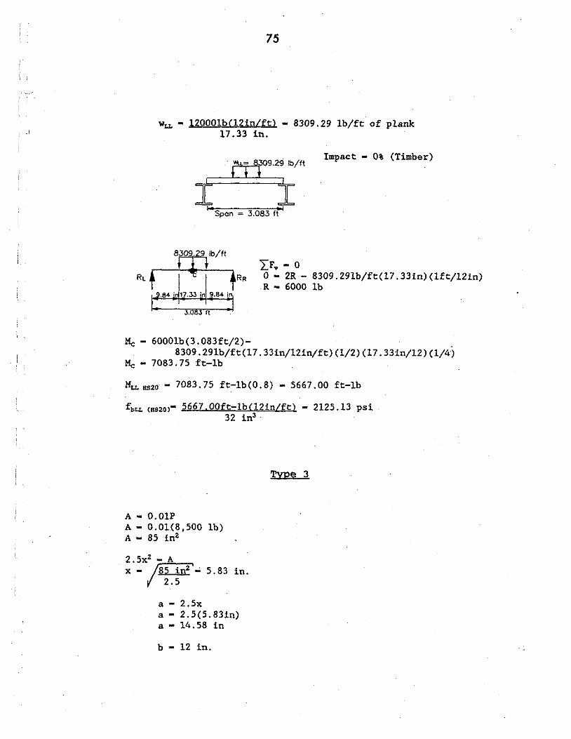
75
wLL • 12000lb(l2in/ft) - 8309.29 lb/ft of plank 17.33 in.
rn309.29 lb/ft Impact • Oi (Timber)
t t .....,.. __ ~=-"'~
Span ~ 3.083 ft
8309.29 lb/ft
l:F .. - 0 RLt m tRR 0 - 2R - 8309.29lb/ft(l7.33in)(lft/12in)
R - 6000 lb .84 · 17.33 in 9.84 in
Mc - 6000lb(3.083ft/2)- . 8309.29lb/ft(l7.33in/12in/ft)(l/2)(17.33in/1,2)(1/4)
Mc - 7083.75 ft-lb
MLL BS20 - 7083. 75 ft-lb(0.8) - 5667 .00 ft-lb
fbLL <as2oi• 5667. 00ft-lb<l2in/ft) - 2125 .13 psi 32 in3 ·
A - O.OlP A - 0.01(8,500 lb) A - 85 in2
2.5x2 - A x - /85 in2 '..; 5.83
2.5
a - 2.5x
in.
a - 2.5(5.83in) a - 14.58 in
b - 12 in.
Type 3

HS20
76
wLL - 8500lb<l2in/ft) - 6995. 89 lb/ft of plank 14.58· in
RL f +RR 1.2 · .58 in 11.21 i
LF,, - 0 0 - 2R -6995.89lb/ft(l4.58in)(lft/12in) R - 4250 lb
Mc - 4250lb(3.083ft/2)-6995.89lb/ft(l4.58in/12in/ft:)(l/2)(14.58in/12)(1/4)
Mc - 5261.15 ft-lb
MLL TYP<t 3 - 5261.15 ft-lb(0.8) - 4208.92 ft-lb
fbLL <TVP• 3)- 4208. 92ft-lb<l2in/ft) - 1578 .. 35 psi 32 in3
RATING
INVENTORY = RATING
OPERATING = RATING
(1450 11si - 13, 07 11si) (36T) 2125.13 psi
(1929 11si - 13. 07 11si) (36T) 2125.13 psi
Values do not control rating; rating controlled by stringer (See Example 6)
= 24.3 tons
= 32.5 tons
LOAD POSTING
TYPE 3 = 1929 11si - 13.07 11si (25T) = · 1578. 35 psi
Values do not control rating; rating controlled by stringer (See Example 6)
30.3 tons
---·· I . )

77
3.3.6.8. Example 8: Rating of timber deck (3 in. x 12 in.)
GIVEN
same as Example 6 (since txample 6 controls over Example 4) with 3 in. x 12 in. transverse plank deck.
Check Rating for deck.
DEAD LOADS
Span Length = (3ft-4in) - 6in + l/2(6in) ~ (3ft-4in) - 6in + 3in
Span Length = 3 ft-l in. = 3.083ft
WPLANK =(3inC12in~ )(50 lb/ft3) 144 in
WROCK =(2inCl2in}) (120 lb/ft3) 144 in2
Mol = (l/8) (32.50 lb/ft) (3.083ft)2c0.8)
Mot = 30.90 ft-lb
Sb= l/6(12~n~ (3in)2 Sb = 18. 00 in
fllDL = M,,l = (30.90 ft-lb} (12 in/ft} S. 18 in5
b
fllDL = 20. 60 psi
LIVE LOADS
fbl.L(HS20J = 5667.00 ft-lb(l2 in/ft) 18.00 in3
fbl.l(TYPE 3) = 4208.92 ft-lbC12 in/ft} · 18.00 in3 ·
WDL
= 3 ft-1 in. controls = 3 ft-l in.
= 12.50 lb/ft
= 20.00 lb/ft
= 32.50 lb/ft
= 3778.00 psi
= 2805.95 psi

HS20 RATING
INVENTORY RATING
78
= /J.450 psi - 20.60 psl\ (36T) \ 3778.00 psi J
= 13.6 tons
13.6 tons rating for deck> 12.9 tons rating for stringer (Example 6)
HS20 INVENTORY RATING = 12.9 tons
Stringer Controls
OPERATING = (1929 psi - 20. 60 psi ) ( 36T) RATING 3778. 00 psi
= 18.2 tons
18.2 tons rating for deck< 19.3 ton rating for stringer (Example 6)
LQAD POSTING
TYPE 3 =
HS20 OPEBATING RATING = 18.2 tons
Deck Controls
(1929 psi - 20.6? psi) (25T) =
2805.95 psi 17.0 tons
17.0 ton rating for deck - 17.0 ton rating for stringer (Example 6)
POST FOR 17 tons
Stringers and Deck control equally.
/ "'- I . )
I
I
1
J

79
3.3.6.9. Example 9: Rating of laminated timber deck (2 in. x 4 in.)
GIVEN
Same as Example 6 (since Example 6 controls over Example 4) with 2 in. x 4 in. continous nail laminated deck.
Check Rating for deck.
DEAD LOADS
Determine member size as described in AASHTO 3.25.1.l
15in + floor thickness = 15 in. + 4 in. = 19 in.
-~-19 in I
Sb=(l/6) (19in) (4in) 2 = 50.67 in3
span Length = 3.083ft (see Example 7)
WDECK = ~ 19inC4inl )(50 lb/ft3)
144 in2/ft2
WROCK =( 19inC2inl )<120 lb/ft3)
144 in2/ft2
WDL
°MoL = (1/8) (58.06 lb/ft) (3,083ft) 2 (0.8)
KnL = 55 .19 ft-lb
fbDL = Mt,L = (55.19 ft-lb)(l2 in/ft) Sb 50. 67 in3
fbDL = 13. 07 psi
= 26.39 lb/ft
= 31. 67 lb/ft
= 58.06 lb/ft

LIVE LOADS
fbl.l(HS20)
80
= 5667.oo ft-1b*c12 in/ft> 50.67 in3
fbl.l(TYPE 3) = 4208 • 92 ft-lb* (12 in/ft) 50.67 in3
*(see Example 7)
HS20 RATING
INVENTORY RATING
= (1450 psi - 13.07 psi) (36T) 1342 .10 psi .
OPERATING = {.1929 psi - 13.07 psi) (36T) RATING \ 1342 .10 psi .
= 1342.10 psi
= 996.78 psi
= 38.5 tons
51.4 tons
vaiues do not control rating; rating controlled by stringer -(See Example 4)
LOAD POSTING
TYPE 3 = (
1929 psi - 13.07 psi) (25T) 996.78 psi
= 48.1 tons
Value does not control rating; rating controlled by stringer -(See Example 6)
I i I

81
3.3.6.10. Example JO: Rating of layered timber deck
GIVEN
Same as Example 6 with layered deck, 3 in. x 6 in. @ 15 in. transverse planks and 3 in. x 12 in. adjacent longitudinal planks.
Check rating for deck planks.
LONGITUDINAL PLANKS
I p (In direction of spon, wheel lood considered f point lood MSHTO 3.23.2. 1)
3 x 12 LONGITUDINAL
3x6 3x6 Normal to direction of span. Wheel load distributed through width of plank - 12 in. (AASHTO 3.25.2.2)
Span· = Clear Distance ~ Clear Span + 1/2 beam width + floor thickness
Span = 9in + 1/2(6in) = 12in ~ 9in + 3in = 12in = 1 ft
Longitudinal Dead Load
WPLAHK = ( 3in(l2in} ) (50 144 in2/ftZ
lb/ft3) = 12.50 lb/ft
WROCK = ( 2in (12in} ) (120 lb/ft3) = 20.00 lb/ft 144 in2/ft2
WDL = 32.50 lb/ft
My,l = (80%) (1/8) (32.50 lb/ft) (1 ft) 2
My,l = 3.25 ft-lb

82
section Modulus; Longitudinal plank
I · 12 in ·I Sb= (l/6) (l2in) (3in) 2
Sb = 18.00 in3
f 0L = 3. 25 ft-lb (12 in/ft) 18.00 in3
= 2.17 psi
Longitudinal Live Load
l\L(HS20) = 80%(PL/4) = 0.8(1200)(1 ft) = 2400 lb-ft 4
l\L(TYPE 3) = 0.8(8500) (1 ft) = 1700 ft-lb 4
fbLL(HS20) = 2400 lb-ft (12 in/ft) = 1600. 00 psi 18.00 in3
fbLL(TYPE 3) = 1700 ft-lb (12 in/ft) = 1133.33 psi 18.00 in3
Longitudinal Rating/Posting
HS20: · INVENTORY = (1450
RATING psi - 2.17 psi) (36T)
1600 psi
OPERATING= (1929 psi - 2.17 psi) (36T) RATING · 1600 psi
= 32.6 tons
= 43.4 tons
TYPE 3 = (
1929 psi - 2.17 ps~\ (25T) = 42.5 tons 1133.3 psi J
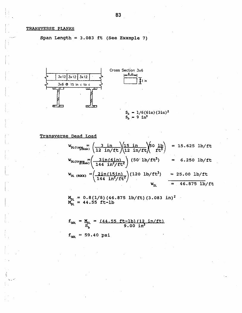
..... ··'
"· - ,.
83
TRANSVERSE PLANKS
Span Length = 3.083 ft (See Example 7)
3x12 .3x12
Transverse Dead Load
Cross Section .3x6 I• sin •I
I 113 ;"
~ - l/6(6in)(3in) 2
~ - 9 in3
w0L 1 = ( 3 in °'1{J.5 in \/so lb) < ~.1.n1<> 12 in/ft J\12 in/ftA ft3°
WDL(trans .·=( 3inC6inl ) (50" lb/ft3) PUU) 144 in2/ft2
WDL (ROCK) ={. 2inC15inl ) (120 lb/ft3) \ 144 in2/ft2
= 15.625 lb/ft
= 6. 250 lb/ft
= 25.00 lb/ft
= 46.875 lb/ft
l\L = 0.8(1/8) (46.875 lb/ft) (3.083 in)2 l\L = 44.55 ft-lb
ftj)L = Hol = (44. 55 ft-lb) (12 in/ft) Sb 9.00 in3
ftj)L = 59. 40 psi

84
Transverse Live Load
Distribution of wheel load
Surface plan area of wheel load on transverse plank
HS20:
LFv - 0 R - 6000 lb
/" " ;, ·1 I· I TRAFFIC 6 inf
1.042 f
WLL(HS20) - 12000lb(l2 in/ft) - 12000 lb/ft 12 in
WLL(Type 3)- 8500lb(l2 in/ft) - 8500 lb/ft Ro 12 in
Mc - 6000lb(3.083ft/2)-12000(lft/2)(lft/4) Mc - 7749 ft-lb
MLL(HS20) - 0.8(7749ft-lb) - 6199.20 ft-lb
fbLL(HSZO) - 6199. 20ft-lbCl2 in/ft) - 8265. 60 psi · 9 in3
TYPE 3:
~) .. - 0 R - 4250 lb
Mc - 4250lb(3.083ft/2)-8500(1ft/2)(lft/4) Mc - 5488.88 ft-lb
MLI.CHS20l - 0.8(5488.88ft-lb) - 4391.10 ft-lb
fbLI.(HSZO) - 4391. l0ft-lb(l2 in/ft) - 5854. 80 psi 9 in3

85
Transverse Rating/Posting
HS20: ( INVENTORY = 1450
RATING psi - 59.40 psi) {36T)
8265.60 psi
OPERATING = (1929 psi - 59.40 psi) {36T) RATING 8265. 60 psi
= 6.1 tons
= 8.1 tons
TYPE 3 = (1929 psi - 59.40 psi). (25T) = 8.0 tons 5854.80 psi
RATING
I.Qngitudinal Transverse ** stringer Plank Plank Controlling
HS20 Inventory 12.9 T 32.6 T 6.1 T 6.1 T
HS20 . Operating 19.3 T 43.4 T 8.1 T 8.1 T
TYPE 3 16.8 T 42.5 T 8.0 T 8.0 T
Post for 8 Tons.
** This indicates that the deck analyzed in this example should be modified to at least the capacity of the stringers or replaced with one of the decks described in the previous examples.

86
The bridge engineer must compare three alternatives when evaluating a deficient bridge: 1) replace the
existing bridge, 2) rehabilitate or strengthen the existing bridge, or 3) leave the bridge in present condition.
To make a rational decision among these three alternatives, the engineer must take several factors into accounL
These factors include: 1) budgetary constraints, 2) potential benefits to the community, and 3) elimination of
a safety hazard. Although many of these factors require qualitative analysis, a rational decision based on
economic factors, can be made by quantifying the dollar value of each alternative and selecting the one which
is the most cost-effective over the life of the structure.
3.4.1. Background
Review of existing literature indicated that several economic evaluation methods have been used in the
pasL The NBI program established a numerical sufficiency rating for each bridge in the United States to
determine its eligibility for federal funding for rehabilitation or replacemenL The tremendous amount of
information resulting from the inspection of the nation's bridges for the NBI program has necessitated a
system for prioritizing bridge rehabilitation and replacement on a national basis. A program has been
developed by the North Carolina DOT which ranks bridge replacement and rehabilitation projects on the basis
of deficiency points accumulated in the NBI inspection and rating process (33). While this prioritizing is useful,
it does not determine the most cost-effective solution to the problems of a particular bridge.
The B/C ratio method has been used in numerous engineering economic analyses to evaluate alternatives.
This method was especially useful because it not only determines which alternative is the most cost-effective,
it also prioritizes the remaining alt(lrnatives. After serious consideration, the B/C ratio method was rejected
for this study because of the difficulty in quantifying the potential benefits of bridge rehabilitation or
replacemenL
A life-cycle cost method has been used in numerous studies to develop cost-effectiveness decision-making
tools for bridge engineers (91). In these methods, a series of cash Dows is converted to a common reference
by the use of the time-value of money equations. According to Winfrey (93), there are four types of life-cycle
analysis methods: 1) the equivalent uniform annual cost method, 2) present worth of costs method, 3)
C9uivalent uniform and annual net return method, and 4) net present value method.
One problem with a life-cycle cost analysis is the difficulty in determining the future costs associated with
a particular alternative. For example, some bridge strengthening methods may require more and different types
of maintenance than other methods performed at the same time. The development of comprehensive bridge
management systems by state DOTs should help to alleviate this problem in the future. Bridge management
systems are presently being developed and these results will become available in the near future (61).
A significant amount of research has been applied to the use of value engineering in the design and
construction of low volume road bridges. Value engineering is defined as "the systematic application of
recognized techniques which identify the function of a product or service, establish a monetary value for that
i f
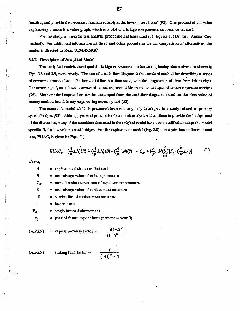
87
function, and provide the necessary function reliably at the lowest overall cost• (90). One product of this value
engineering process is a value graph, which is a plot of a bridge component's importance vs. cost
For this study, a life-cycle test analysis procedure has been used (ie. Equivalent Urtiform Annual Cost
method). For additional information on these and other procedures for the comparison of alternatives, the
reader is directed to Refs. 10,34,45,59,87.
3.4.2. Deaaiptlon of Ana1ytlcal Model
The analytical models developed for bridge replacement and/or strengthening alternatives are shown in
Figs. 3.8 and 3.9, respectively. The use of a cash-flow diagram is the standard method for descn1ling a series
of economic transactions. The horizontal line is a time scale, with the progression of time from left to right
The arrows signify cash flows -downward arrows represent disbutsementsand upward arrows represent receipts
(75). Mathematical expressions can be developed from the cash-flow diagrams based on the time value of
money method found in any engineering economy text (53).
The economic model which is ptesented here was originally developed in a study related to primary
system bridges (95). Although general principals of economic analysis will continue to provide the background
of the discussion, many of the consid.erations used in the original model have been modified to adapt the model
specifically for low volume road bridges. For the replacement model (Fig. 3.8), the equivalent uniform annual
cost, EUAC, is given by Eqn. (1).
EUAC, = (A ,i,N)(R) .:. (A ,i,N)(B)- (A ,i.N)(S) +Car+ (A ,i.N)t [F1 • (p ,i,n)J (1) P P F P 1-1 F
where,
R = replacement structure first cost
B = net salvage value of existing structure
C,, = annual maintenance cost of replacement structure
S = net salvage value of replacement structure
N = service life of replacement structure
= interest rate
Fµ = single future disbursement
n; = year of future expenditure (present = year 0)
(NP,i,N)
(NF,i,N)
capital recovery facior ~
= sinking fund factor =
i(1 +l)N
(1 +i)N - 1

88
R Fi•C ar F k + C ar R
i C ar
8 n s
n
N
Fig. 3.8. Economic model for replacement alternatives.
I

I
D
[ '
F ' c i as
C as
n
n k
89
F k' C as
N
R
!c
8
a r
Fig. 3.9. Economic model for strengthening alternatives.

90
(P/F,i,n;) = present worth of a future sum = 1
(1 +i)"'
Salvage values can be either positive or negative. In most cases, little salvage value remains in an existing
bridge, and the bridge owner must pay for the removal of the bridge. This removal cost must be represented
as a negative salvage value in the EUAC equations. If N is assumed to be very large (e.g. > SO years) and B
to be relatively small compared to R, Eqn. (1) can be simplified to Eqn. (2).
EUAC, = ("4. ,1,N)(R-S) + C,,,+ (S-B)i + (~.i,NfE [Fj · (P ,i,n1)1 p P1•t F
(2)
There are two significant advantages to using Eqn. (2) rather than Eqn. (1). In most cases, the removal
cost of the existing structure, B, will be approximately that of the replacement structure, S. Therefore, the (S·
B)i term becomes insignificant and can be ignored. In addition, the bid price of the replacement structure
norma11Y includes the removal cost of the existing structure. If this is the case, the (R.S) term in Eqn. (2) will
be the total bid price of the replacement structure (95).
To develop an economic mOdel to represent the bridge strengthening procedure, two significant
assumptions must be made. Fust, money spent to strengthen an existing bridge only benefits the existing
structure. Therefore, disbursements made to strengthen the existing bridge must be evaluated only over the
remaining life of the existing bridge. Secondly, after the existing bridge is eventuallY replaced, all costs are
considered to be common to both the replacement and strengthening mOdeL
(3).
where
The mathematical mOdel to represent bridge strengthening or rehabilitation (Fig. 3.9) is shown in Eqn.
D
c .. N'
(A!P,i,N')
EUAC, • (.!!.,1,N~(D) + C., + (A ,l,N~t [F1 • (p ,i,n)J P. P J·1 F
=
= =
=
=
=
initial cost of strengthening existing bridge
annual maintenance cost of existing structure after strengthening
remaining service life of existing bridge
single future disbursement
year of future disbursement
capital recovery factor = i(1 +J)N
(1 +i)(N-1)
(3)
i ,,..,.-.,,, I
l'
,.,.-. .__

91
= present worth of a future sum = 1
(1 +i)"'
A brief description of the variables included in the economic models for bridge strengthening and
replacement follows. A database of estimated prices is presented in Sec. 3.7 of this report for various
replacement methods.
3.4.2.1. Replacement Structure Fust Cost (R)
The first cost of a bridge replacement structure has the greatest effect on the EUAC of any of the
factors. Fortunately, the first cost of a bridge is the easiest factor to quantify accurately. There are at least
four considerations which can significantly effect the first cost of a replacement bridge:
• Span length: In general, the cost per ft2 of a new bridge tends to increase with longer span lengths.
Low volume bridges tend to have much shorter spans, making this variable less significanL ·
• Roadway realignment: Alignment changes in low volume roads, and thus bridges, are less frequent
than in a more highly traveled roadway.
• Environmental studies and potential consequences: The effect of a low volume bridge replacement
project on the environment tends to be of a localized nature, which limits the relevance of this
variable.
• Construction of temporary detours: The construction of temporary detours would be infrequent on
low volume roads. Usually there are a small numberof users being inconvenienced, thus most likely
the existing road would simply be closed during construction of a new bridge.
3.4.2.2. Structure Service Life (N,N?
It is common practice to assign a service life of SO years to new bridges in an economic analysis. This
common 'rule-of-thumb' may be influenced by the geographical and climatological location of the proposed
bridge, however. Factors which affect the service life of a new bridge are 1) the quality of the initial design,
2) the quality of materials used ii: construction,3) the quality of workmanship used in construction,4) the level
of routine maintenance perfortned on the structure during the life cycle, and 5) the severity of the climate.
The remaining service life of an existing structure is most often estimated by an engineer after completing
an inspection and thus is very difficult to quantify accurately. There are very few detailed guidelines available
for this purpose, and it may be difficult to avoid personal bias in the estimate.
3.4.2.3. Interest Rate (1)
Historically, long term economic analyses of public works projects have ignored the effect of inflation on
the interest rate used in computing equivalent costs. Cady has determined that, due to the present national
economy, inflation must be considered in any life-qcle cost analysis (14).
A relationship which accounts for the difference between the rate of inflation and the nominal interest
rate is presented in Eqn. (4):

where
io = real or effective interest rate
92
1 + i io = ..:___z - 1 1 +y
(4)
~ y
= =
nominal interest rate (usually based on high-grade municipal bonds)
rate of inflation (usually based on changes in the consumer price index)
Jn general, a higher nominal interest rate tends to favor future expenditures (e.g. present strengthening
with possible future replacement), while a lower nominal interest rate favors the larger immediate capital
investment (e.g. immediate bridge replacement) (93).
3.4.2.4. Bridge Maintenance Costs (C.,, Cu)
The most difficult factor to predict in any economic model is the annual maintenance costs of the bridge,
both as it exists today, and after any strengthening or rehabilitation work.
Large, one-time, maintenance expenditures, such as a bridge deck overlay, should not be included in the
C., and c .. terms. These types of expenses are represented by the single future disbursement terms, F; and
Fb in Figs. 3.8 and 3.9 and should be converted to a present worth by the present worth of a future sum
equation and then to an EUAC by the capital recovery factor.
3.4.2.5. Bridge Removal Costs (B,S)
Several factors which can significantly affect the cost of bridge removal are: superstructure type, span
length, number and type ofabutments, depth of removal below ground line, and any environmental precautions
which must be taken.
Klaiber, et. al have shown that bridge width is not a significant factor in estimating removal costs (36).
As mentioned earlier, one advantage of using Eqn. 2 rather than Eqn. 1 to model the replacement of a bridge
is- that both B and S can be ignored.
3.4.2.6. Level of Service Factor ~)
The Level of Service Factor, LS, was introduced by Wipf, et. al (95) as a means of quantifying the
economic benefits a road user would reali7.e with the construction of a new bridge. A new bridge can be
expected to provide reduced accident rates, reduced traffic delays, a reduction in detour mileage for trucks
which exceed the posted load limit and other intangible Sa.vings over an existing bridge. These reductions are·
an additional cost of keeping an existing bridge in service and are represented as an additional cost in the
strengthening alternative.
In previous studies by McFarland ( 45), the .traffic accident rate at the bridge site is related to the roadway
approach width and the bridge width. A reduction in accident rate which could be expected with an increase
in bridge width has been calculated.
"

93
The present study on low volume road bridges required a modification of the level of service factor
previously defined. Tne three considerations in !he level of service factor, reduced accident rate, reduced traffic
delay, and reduced detour length do not apply in a low ADT environment. Since !here is very little traffic, it
is unlikely that a traffic delay will occur due to existing bridge conditions. Similarly, since there is so little
traffic, there can be very few accidents which occur on the existing bridge. The reduction of already small ,.
accident rates is statistically insignificant. Finally, the concept of a detour length due 10 an understrength bridge
is difficult to define. There are so few users of a particular bridge that, at least in most cases, it would not be
a significant inconvenience to require a detour to the next county road (usually located one mile away).
3.4.2. 7. Other Considerations
In addition to the variables in the economic model, the practicing engineering must take other
considerations into account when making decisions regarding bridge rehabilitation or replacement. These
considerations are usually very difficult to quantify. The engineer should not allow personal desires to
completely override the decision making process. The most cost-effective solution, as determined by the EUAC
method, should not be discarded due to the dislike of the particular procedure. The quantifiable 'best•
alternative should, however, be reviewed with sound engineering judgement.
3.4.3. Nonnal Distribution and EUAC Simulation
The economic model presented represents a simulation of possible outcomes. The· service life of a
particular alternative and the nominal interest rate used for calculations are not certain. . To determine the
range of possible outcomes, probability theory can be used for these variables.
The normal probability distnoution of variables is well .known and simple to apply. For this discussion
it is assumed that the service life arid nominal interest rate are normally distrtl>uted. There are several tests
available which allow the user to determine whether a particular data set is normally dismouted (18).
3.4.3.1. NormaJProbability Distn1Jution
The normal probability di.strtoution, also known as the Gaussian distnoution, is the most frequently
encountered probabilitydistnoution. The normal dismbutioni.s recogni7.ableas the familiar 'bell-shaped curve•
(see Fig. 3.10). Two parameters completely descnbe a particular normal curve: the mean, µ,which locates
the center of the curve, and the standard deviation, o, which provides a measure of the degree of dispersion.
The height of a normal curve above any point along the horizontal axis is the relative frequency. This height
can be descnoed by:
1 -~ J(x) = --e 2"'
./2tto
Every normal frequency curve is centered on the mean. The tails of the curve taper off rapidly for values of
x very far from the mean; The area under the normal curve betweenµ. and any point depends only on the

94
, I . I )
o.o
O.H
0. l 5
0. l 0
>- 0. 15 I-..... ....J ..... co c( 0. 1 0 co 0 er: c..
0 . 1 5
0. 1 0
0.05
0.00 ·l.00 • 2. 0 0 • 1. 00 0. 00 1. OD 2.00 l. 0 0
NORMAL OEVIATE,Z
Fig. 3. 10. Normal probability. distribution.

( ....
95
distance separating that point and the mean, as expressed in units of a. This distance from the mean is known
as the normal deviate, designated as z.
Since a normally distnl>uted variable is continuous, probabilities for an event X can be found by using:
• 1 _.!l:J!i F(x) = Pr{X ,; .xJ a f e 2 ..
-./2ia
This integral is rather complicated to compute. Fortunately, any statistics manual contains of table of
cumulative probability values for tbe normal distnbution (39).
For purposes of this economic model, we shall consider only those events which occur within 3 standard
deviations of the mean, that is: -3.00 s z s +3.00. This region of tbe normal distnbution includes 99.73
percent of all possible events.
3.4.3.2. Simulation of EUAC Results
To simulate the uncertainty in possible results of an EUAC calculation, the region between z = :!:3 has
been divided into 25 intervals. Each interval represents 4 percent of the total area under the normal
probability curve. These intervals are essentially the 0th, 4th, 8th, etc. percentile of possible outcomes. The
z value for the endpoint of each interval .is computed, and converted into a value of service life and interest
rate. For example, the 0th percentile is equivalent to a z value of -3.00, the 4th percentile is equivalent to a
z value of-1. 76, etc. These possible values of service life and interest rate are arranged in an array of possible
outcomes. There are 625 possible outcomes (25 x 25 = 625), each of which has a unique value of service life
and interest rate. The EUAC for each possible outcome is computed, and various statistics (mean, standard
deviation, high, and low) are computed based on these outcomes.
The user must be aware that there is no one correct answer to the EUAC comparison of alternatives.
It is expected that the actual EUAC of a particular alternative will range between the high and low values as
determined by the computer simulation. This range of possible outcomes must be considered in the
comparison of possible alternatives.
3.4.4.. Compu11lr Spreadsheet for EUAC Comparlson
A computer spreadsheet has been developed to simplify the calculations of EUAC for various bridge
alternatives. In addition, this spreadsheet has been designed to allow the user to simulate the effect of various
service lives and nominal interest rates on the EUAC of these alternatives. The EUAC spreadsheet (developed
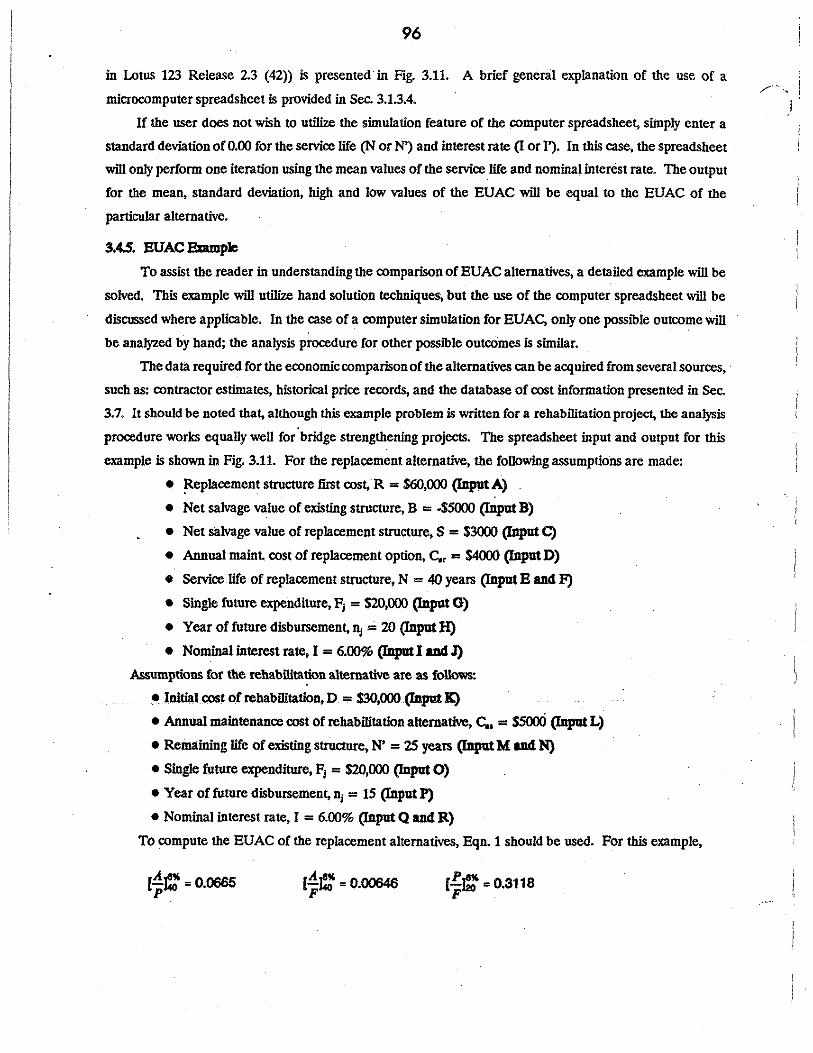
96
in Lotus 123 Release 2.3 (42)) is presented in Fig. 3.11. A brief general explanation of the use of a
microcomputer spreadsheet is provided in Sec. 3.1.3.4.
If the user does not wish to utilize the simulation feature of the computer spreadsheet, simply enter a
standard deviation of 0.00 for the service life (N or N') and interest rate (I or I'). In this case, the spreadsheet
will only perform one iteration using the mean values of the service life and nominal interest rate. The output
for the mean, standard deviation, high and low values of the EUAC will be equal to the EUAC of the
particular alternative.
3.4.S. EUAC Elample
To assist the reader in understanding the comparison of EUAC alternatives, a detailed example will be
solved. This example will utilize hand solution techniques, but the use of the computer spreadsheet will be
discussed where applicable. In the case of a computer simulation for EUAC, only one possible outcome will
be analyzed by hand; the analysis procedure for other possible outcomes is similar.
The data required for the economic comparison of the alternatives can be acquired from several sources, ·
such as: contractor estimates, historical price records, and the database of cost information presented in Sec.
3.7. It should be noted that, although th.is example problem is written for a rehabilitation project, the analysis
procedure works equally well for bridge strengthening projectS. The spreadsheet input and output for this
example is shown in Fig. 3.11. For the replacement alternative, the following assumptions are made:
• ~eplacement structure first cost, R = $60,000 (Input A)
• Net salvage value of existing structure, B = -$5000 (Input B)
• Net salvage value of replacement structure, S = $3000 (Input C)
• Annual mainL cost of replacement option, C., = $4000 (Input D)
• Service life of replacement structure, N = 40 years (Input E and F)
• Single future expenditure, Fi = $20,000 (Input G)
• Year of future disbursement, n1 =' 20 (InputH)
• Nominal interest rate, I = 6.00% (Input I ud J)
Assumptions for the rehabilita~n alternative are as follows:
• Initial cost of rehabilitation, D = $30,000 (Input K)
• Annual maintenance cost of rehabilitation alternative, C.. = $5000 (Input L)
• Remaining life of existing structure, N' = 25 years (Input M ud N)
• Single fµture expenditure, FJ = $20,000 (Input 0)
• Year of future disbursement, n1 = 15 (Input P)
• Nominal interest rate, I = 6.00% (Input Q and R)
To compute the EUAC of the replacement alternatives, Eqn. 1 should be used. For this example,
r;i: = o.00646

97
Cost-Effective Comparison of Alternatives
Press <ALT> A at any time to update the iterative module!
Replacement Alternative Input:
Replacement Structure First Cost, R =
Net Salvage Value of EXISTING Structure, B =
Net Salvage Value of REPLACEMENT Structure, S =
Annual Maintenance Cost of New Structure, Car =
Service Life of Replacement Structure:
Mean value= ,__ __ 4~0'"'1 years E
Standard deviation = '-----'O'-'I years F
Single Future Expenditure, Fj = ·
Year of Future Expense (current year= 0), Nj =
Interest Rate, l:
Mean value=
Standard deviation =
EUAC of Replacement Alternative:
Mean value of EUAC =
Std. Dev. of EUAC =
High value of EUAC =
Low value of EUAC =
6.00%1
0.00%\ J
$8,715
$0
$8,715
$8,715
Note: Numerical value in parenthesis for input B Indicates negative number.
$60,0001 A
· ($5,000X B
$3,0001 c
$4,000 I per year D
$20,000I G
201 H
Fig. 3. 11. Economic analysis spreadsheet, input parameters, and example problem.

98
Rehabilitation/Strengthening Alternative Input:
Initial Rehabilitation/Strengthening Cost, 0 = $30,000\ K
Annual Maintenance Cost After Rehab/Siren, Cas = $5,000 lper year L
Remaining Service Life of Existing Structure, N':
Mean value = 25 I M
Standard deviation = o I N
Single Future Expenditure, F'j = $20,000 I 0
Year of Future Expenditure (current= 0), N'j = 15 I P
Interest Rate, I:
Mean value=
Standard deviation =
EUAC of Rehab/Strengthening Alternative:
Mean value of EUAC =
Std. Dev. of EUAC =
High value of EUAC =
Low value Of EUAC =
Fig. 3. 11. Continued.
6.00%1 Q
0.00%1 R
$8,000
$0
$8,000
$8,000
I. I,
.··"';,.

as:
99
When these factors are included in Eqn. 1, the EUAC of the replacement alternative can be computed
EUACR = 0.0665(60,000-(-5000)] - 0.00646(3000)+ 4000 + 0.0665{20,000(0.3118)) = $8717
Tue EUAC for the rehabilitation/strengthening model can be computed from Eqn. 3. In this example,
[Ai:' = 0.0782 p [~ft:= 0.4173
When these factors are inserted into the Eqn. 3, the EUAC. can be computed as:
EUAC, • 0.0782(30,000) + 5000.,. 0.0782(20,000(0.04173)) = $7999
For the above example, the EUAC of the replacement alternative was slightly more than the EUAC of
the strengthening alternative. Thus, considering only EUAC's, one would select the
rehabilitation/strengthening alternative.
The user must be aware that the actual difference between the two alternatives may be less than the
error in estimation of one or more of the terms in the equations. Sound engineering judgement must be used
in the interpretation of the results.
3.5. Strengthenlng Technlques for Steel Stringer Bridges (FHW A 302)
3.S.1. Replacement of Damaged Stringers
A bridge's load carrying capacity can be increased by replacing.damaged or deteriorating stringers. It
may not be necessary to remove the deck even if the deck and stringers are panially or fully composite. A
procedure for such a replacemenc is described in the NCHRP 222 report (84). Traffic should be detoured to
allow jacking of the bridge to provide clearance between the beam and the end supports. The web of the
. damaged beam should then be cut at the junction of the top flange and web (see Fig. 3.12). The elCpOsed face
of the flange, which remains· in the concrete, needs to be ground flat The width of the top flange of the
replacement beam should be slightly less than that of the original beam to facilitate field welding. Using . . continuous fillet welds, the new steel beam is connected to the top flange of the original beam. If required,
cover plates can be welded (preferably, shop welded rather than field welded) to the bottom flange of the new
stringer prior to field installations to lower the neutral axis thus reducing lower flange stresses. In situations
where it is necessary to replace a non-composite stringer with a composite stringer, the previously descnl>ed
procedure is not applicable. In these situations, a steel stringer can be added and made to act compositely with
the concrete deck without remoVing a portion of the deck by coring through the existing deck and adding shear
·connectors. Pressure grouting through either the cored holes in the deck or from below can be used to fill the
voids between the deck and stringers.

, /
pt::.;. P:. ~:: :·.r .... :.::.~:··r·'-:;: .. :.~ .. .:··1v. ... : · ·: · .. <I ::~·:= .. :.,. .. ;: .. : .. ; .. ~~~::·:~:-·l3" · n-· -.:-. · .· \:.;..: .. ::: .... :.: .. ::~:~:: .. : .. :1 · :· · :.r. ·.I I I I i\k
!;; I;::
!:: !;; 'I
t::
!;;
'----!Burn to remove lower portion of beam and grind smooth
')
'I
Damaged or deteriorated steel beam stringer
.. -.4 ·" · ~ r, . .:.f.;.~..: .. :..-:::-::·1 ·.t:;-: .. : : • ·17 f·:·:,:.,: .. :~:~.~-::.~~:~~;:.~: t>·. ·. ·. · : : : ~-:~!~-~:::_.:::~:~:.~;: .... ;.: .... ;~ ·:· : .'. "?.
Fig. 3. 12. Steel beam replacement.
'-weld new stringer to old stringer top flange for continuity
Vi New stringer
~---Optional cover plate
-0 0
/.~ ,
""

101
The Iowa DOT V9, Vll and V13 standards for steel stringer bridges specified smaller, lower capacity
exterior stringers lltan those used for the interior stringers. Replacement of these external stringers with
stringers the same size as the internal stringers (or slightly larger) can provide additional strength for the
existing bridge. However, more cost effective procedures for strengthening these bridges will be presented in
the following sections.
3.S.2. Respadng Emling StdngeII and Adding New Strlngcn
3.5.2.1. Background
Generally, the res pacing of existing stringers and adding new stringers (henceforth referred to as respace
and add) is implemented to increase the flexural strength of the bridge by reducing the spacing between the
stringers. For most applications, removal of the existing deck is required. In these cases, the live load capacity
of the bridge can be further increased by replacing the original deck with a lightweight deck. Jn some cases,
the additional stringers can be added to allow for widening of the original bridge, assuming the original
abutments/piers are of sufficient width. In the respace and add procedure, it is important to consider the two
items: 1) to minimize differential deflection between the new stringers and the existing stringers, and to ensure
all stringers carry similar loads, the new stringers should have stiffnesses (i.e. moment of inertias) similar to the
existing stringers, 2) analysis of bridges with nonuniformstringer spacing most likely will require more involved
analysis, such as finite element analysis, thus stringer spacing should be kept uniform if at all possible.
The evaluation procedure required for strengthening steel stringer bridges using the respace and add
method is descnlled in the following paragraphs. The procedure has been simplified by using a computer
spreadsheet. The following example problem (Sec. 3.5.25) has been solved by using hand calculations and by
using the_ computer spreadsheet developed.
3.5.2.2. Design Criteria
Iowa agencies must currently conform to the AASHTOStandard Speciiicationsfor Highway Bridges (2).
The procedure presented in this section, as well as following sections, is based on these specifications.
3.5.2.3. Design Limita lions
The bridge strengthening evaluation only investigates the bridge superstructure. Although not included
in this manual, the substructure should also be investigated before any rehabilitation is undertaken. The
substructure should be inspected for signs of scour, decay and damage. Jf the load carrying capacity of the
superstructure is increased, the capacity of the substructure should be reviewed to deterntine if it is
adequate for the increased loading; in some situations, the substructure may also require rehabilitation. As
a minimum, the following items associated with the substructure should be reviewed:
• Pile axial load capacity,
• Bent/pier capacity for overturning forces, and
• Capacity of abutments, bents and piers.
The following limitations apply t? steel stringer bridges evaluated by the procedure which follows:

102
• All stringers are assumed to have similar material and section properties .
• The superstructure has no or minimal skew. )
• The deck section and material properties are homogeneous. I • Bridge stringers are assumed to be simply supported.
3.5.2.4. Design Procedure
L Detcrmlnc the allowable and operating steel stress lewls. (G and H In the apreadSheet)
Frequently, bridge plans documenting the type of steel in the stringers can not be found. In these
cases, the Iowa DOT recommends allowable and operating steel stress levels based on the year
the bridge was constructed (see Table 3.3).
Table 3.3. Iowa DOT steel stresses based on the year the bridge was constructed.
Year •. Allowable Stress (G) Operating Stress (H) Constructed (ksi) (ksi)
Before 1905 14.30 19.50
1906 to 1936 16.50 22.50
1937 to 1962 18.15 24.75
1963 to 1999 20.00 27.00
2. Detcrmlnc the moment capacity of the Interior atrfngera. (I) This evaluation determines the
moment capacity of the interior stringers based on the allowable stresses in Table 3.3 and the
section modulus of the interior stringers.
Stringer Moment Capacity = Section Modulus x Allowable Stress
3. Determine the dead load moment capacity of the superstructure. (J) Dead load includes all
permanent loads associated with the superstructure and roadway, including stringers, diaphragms,
deck, wearing surface, fill on gravel roads, railings, sidewalks, barriers, lighting, utility lines carried
by the superstructure, etc. The dead load bending moment a typical interior stringer must
support based on beam theoiy is:
Applied Dead Lead Moment = (Uniform Dead Load x Bridge Lengtli')/8
4. Determine the iiYc load moment capadty of the lillperstructure. (K) The live load the bridge must

103
withstand is based on Iowa legal truck loads. The live load moment capacity of the bridge is the
difference between the stringer moment capacity and the applied dead load moment.
Live Load Moment Capacity =
Stringer Momeni Capacity -Applied Dead Load Moment
S. De11:J:mine the AASHTO liWI load dlstrlbution faclor. (L & M) As previously noted, bridge loads
must be appropriately distnbuted to a single longitudinal stringer for analysis. AASHTO wheel
load distnbution factors for stringers are based on the number of traffic lanes, deck material and
stringer spacing. (See Table 3.23.1 in AASHTO.) Since timber plank and concrete decks are the
prevalent types of decks on lhe deficient bridges identified in the Iowa SI&A survey, they were
both considered in the evaluation spreadsheet. AASHTO wheel load distnbution factors for steel
stringers are given in Table 3.4.
Table 3.4. AASJ:ITO wheel load distnbution factors • steel stringers.
Deck Type One Lane (M) Two Lane (L) .
Timber Plank S/4.5 for 4 in. deck (1) S/4.0 for 4 in. deck (2) S/5.25 for 6 in. deck
Concrete sn.o (3)
S = average stringer spacing in ft. (1) If the spacing, S, exceeds 5.5 ft, use the reaction of the wheel loads. (2) If the spacing, S, exceeds 7.0 ft, use the reaction of the wheel loads. (3) If the spacing, S, exceeds 10.0 ft, use the reaction of the wheel loads. (4) If the spacing, S, exceeds 14.0 ft, use the reaction of the wheel loads.
S/5.5 (4)
6. Detenninc the AASHTO Impact factor. (N) Impact factors account for the fact that loads are not
applied statically. AASHTO impact is a fraction of the live load stress. (See Section 3.8.2 of
AASHTO).
Impact = 50/(Bridge Length (ft) + 125)
I = 50/(L + 125)
This calculated value shall not exceed 30 percent
7. Determine the maximum trudt load moment by hand calculations or from applicable tables. (0)
The truck live loads moments including impact are determined by:

104
where:
• Mu... •• = live load moments with impact factor (in units offoot-kips per wheel line). See
Appendix B for Iowa truck live load moments.
• 2 is for 2 wheel lines
• Dist.u. = live load distnoution factor.
8. Detcrmfne Iowa DOI' legal truck load posting values from the operating rating. (P) The live load
demand (based on the operating stress) is compared with the live load moment capacity to
determine if the bridge requires posting. (See Appendix A for truck weights.)
Operating Rating= (Mu .. ,.or/MU••m•nd) x Truck Weight
The maximum operating rating loads for which a bridge can be posted are presented in Table 3.5.
Table 3.5. Maximum operating rating loads.
Truck Maximum Load (Tons)
Type3 25.0
Type 3S2(a) . 36.5
Type 3S2(b) 40.0
Type4 27.5
Type 3S3 40.0
Type"3-3 40.0
9. Detcrmfne the HS flm:ntory mtlng (for use in c:alculating the SI&A auftidency mtfng). (Q) The
inventory rating used in the appraisal sheet can also be calculated to determine the effect of the . .
proposed strengthening method on the SI&A sufficiency rating. The inventory rating differs fr.om
the operating rating only by the stress used. The NBI coding guide (25) provides the factors
included in the SI&A sufficiency rating. Briefly stated, the sufficiency rating = St + S2 + S3 + S4. The Sl factor refers to the structural adequacy and safety; S2 to serviceability and funetional
obsolescence; S3 to essentially for the public use; and S4 to special reductions which include
detour length, traffic safetY features and structure type. Each of these four factors is a function
of coded items included on the appraisal sheet.
. ' . '
: I

105
. 3.5.2.5. Evaluation of Existing Stringers Example
The following steel stringer evaluation is performed for a 20 ft wide and 20 ft long non-composite steel
stringer bridge. The bridge has five stringers spaced at 3.8 ft. This example follows the procedure outlined
in the previous section. Input, as well as the majority of the calculated intermediate values have been identified
by letters shown next to the spreadsheet cells (year built (A); length (B}; etc.). The spreadsheet input and
output (highlighted on the spreadsheet) for this example is shown in Fig. 3.13.
1. Detmmlnc the allowable and operating steel lltteaa levels. The example bridge (20 ft long (B))
was built in 1955 (A). Therefore, as presented in Table 3.3, the allowable steel inventory stress
is 18,150 psi (G) and the operating/posting stress is 24,750 psi (H).
2. Determine the moment capacity of the Interior stringers. The stringers in this example are steel
S1Sx50 sections with a section modulus of 64.8 in3 (D).
Stringer Inventory Moment Capacity =
( ~·~) x (18.15 l:sl) = 98.01 ft-J: (1)
Stringer Operating Moment Capacity =
( ~8~) x (24.75 l:st) = 133.65 ft-J: (1)
3. Determine the dead load moment capacity of the auperstrllCtme. The weight of the stringers,
deck, wearing surface and barrier is assumed to be 0.4klf. The applied bending moment on a
typical internal stringer is:
. Applied Dead Load Moment =
• (0.4 #'J (20 Jt)2 a 20 ft-J: (J) 8.
4. Determine the live toad moment capacity of the superstructure.
Inventory Live Load Moment Capacity = 98.01 - 20.0 = 78.01 ft-k (K)

106
,,----~~~~~
INlERMEOIA,,.. VALUES n-~IK'SJ~
1s.1e "PERATING STRESS KSI) I 24.75
c D E F
"' H
~oMENT CAPACllY tKlP·r, 1 INVENTORY
OPE~· OTALSTRUCTURE 98.01 1 I DEAD LOAD 20.00 J JVELOAD . 78.01 1 .65 K
•VE LOAD DISTRIBUTION FACTORS 1wOLANESORMORE I 0.6909 L ""'ELANE I 0.5429 M
MPACT FACTOR I 1.3 N
LIVE LOAI' + IMPACT MOMENT 0 21aN~~ 1 L~Nr
1S20 143.71 112.91 TYPE3 123.67 97.17 TYPE.3S2(a) 112.77 88.61 rvPE3S2(b) 123.67 97.17 TYPE4 138.32 108.68
~~3S3 138.32 108.68 E3-3 102.28 80.36
BRIDGE LOAD IN TONS p IKIJCK 2LANES 1 LANE MAX LOAD 1S20 15.82 20.13 20.00 TYPE3 22.97 29.24 25.00 TYPE3S2(a)
~ 32.07 36.50
TYPE3S2(b) 29.24 40.00 TYPE4 26.14 27.25 TYPE'3S3 26.14 40.00 'I TYPE3-3 44.451 35.35 40.00
MAX S.I. & A. RATING Q RUCK 2LANES 1 LANE
HS20 10.86 13.82 . BESTS.I. & A. SUFFICENCY RATING 64.98 70.98 .
Fig. 3. 13. Spreadsheet for steel beam replacement example.

107
Operating Live Load Moment Capacity = 133.65 • 20.0 = 113.65 fl-k (K)
5. Determine the AASHI'O liYc load dlstrib111ion flldor. The deck in this example is reinforced
COI)crete with two lanes of traffic.
L.L. Distribution Facror = ~ = 0.6909 (L) . 5.5
6. Determine the AASHI'O Impact flldor. The bridge length is 20 ft.
I • 50/(L + 125)
I = 50/(20 + 125) = 34% >30% (N)
This calculated impact is greater than the 30 percent limit; therefore, 30 percent impact controls.
7. Determine the maximum truck load moment by hand calculations or from applk:able tables. See
Appendix B for the truck live load moments.
M-*"' = Ml>'W.k x I x 2 x Dist.u (O) ·
• HS20: 104.0 fl·k x 2 x 0.6909 = 143.71 fl-k
• Type 3: 89.5 fl-k x 2 x 0.6909 = 123.67 fl-k
• Type 3S2(A): 81.6 fl-k x 2 x 0.6909 = 112. 77 fl-k
• Type 3S2(B): 89.5 fl-k x 2 x 0.6909 = 123.67 fl-k
• Type 4: 100.1 fl·k x 2 x 0.6909 = 138.32 fl-k
• Type 353: 100.1 fl-k x 2 x 0.6909 = 138.32 fl-k
• Type 3-3: 74.0 fl-k x 2 x 0.6909 = 102.28 fl·k
8. Determine the Iowa DOT legal lrlletload poatlngwlueafromtheoperatlngratlng. The live load
demand (based on the operating stress) is compared with the live load capacity to determine the
load values for posting. (See Table 3.5 for the maximum truck weights and Appendix A for truck
configurations.)
Operating Rating = (Mu -JMu ~ x Truck Weight (P)
• Type 3: (113.65 fl-k/123.67 fl-k) xas ton = 22.97 ton < 25 ton
• Type 3S2(A): (113.65 fl-k/112. 77 ft-k) x 36.5 ton = 36. 77 ton > 36.5 ton

• •
108
Type 3S2(B): (113.65 ft-k/123.67 ft-k) x 40 ton = 36. 76 ton < 40 ton
Type 4: (113.6 ft-k/138.3 ft-k) x 27.25 ton = 22.39 ton < 27.5 ton
• Type 3S3: (113 .. 6 ft-k/138.3 ft-k) x 40 ton = 32.85 ton < 40 ton
• Type 3-3: (113.6 ft-k/102.3 ft-k) x 40 ton = 44.43 ton > 40 ton . I
Required posting for this bridge would be a combination of the following Iowa legal truck types: Type
3 at 23 tons, Type 3S2(B) at 36 tons, Type 4 at 22 tons and Type 3S3 at 32 tons, as is shown in the
output section of Fig. 3.13. The Iowa DOT guidelines for posting non-interstate highways staie the
posted load limit for a straight truck (see Appendix A for truck configurations) may be based on the
Type 4 vehicle. The posted load limit for the semi-trailer combination and the truck plus full trailer
may be based upon, respectively, the Type 3S3 and Type 3-3 vehicles. Other suitable posting schemes,
including those utilizing a triple axle limit sign, may be used in lieu of the descn"bed method when
appropriate. The posted load limit for the triple axle, if such posting is used, shall be based upon the
load rating for the Type 4 and Type 3S3 vehicles. The maximum posting weight for the triple axle is
21 tons.
9. Determine the HS Inventory rating (for usc in cak:ulatfng the SA&I sufficiency rating).
HS20 Inventory Rating (tons)=
(lnw11U1ry 1iW1 load 'moment capacity) JC (Weight of true~
7Tuck 1iW1 load + impact moment
= ( 78·01 ft-k) JC (20 ton) = 10.86 ton (Q) 143.71 ft-k
The NBI coding guide outlines in detail the factors included in the SI&A sufficiency rating. For
comparison purposes, a sufficiency rating could be obtained for this bridge if all factors except the HS truck
loadings are assumed to be •perfect•:
• Adjusted inventory tonnage (AIT) for this HS20 truck = 1.00 x 10.86 = 10.86
• I = (36 -AIT)LS x 0.2778 = (36 - 10.86)1.5 x :1.778 = 3S.01
• SI = SS - (A + B + C + D + E + F + G + H + I)
(Assume no reductions for A through H.)
SI = SS - 35.02 = 19.98
• Sufficiency rating = Sl + S2 + S3 + S4
(Assume S2, S3, and S4 are 'perfect')
Sufficiency rating = 19.98 + 30 + 15 = 64.98.
i r

109
Note that it is highly unlikely that 'perfect• factors actually exist Therefore, this is a hypothetical SI&A
sufficiency rating for ti.I.is bridge.
3.5.26. Respace and Add Stringer Example
To demonstrate how respacing and adding stringers increases a given bridge's capacity, the same bridge
is re-evaluated with several different stringer spacings (and number of stringers). Shown in Fig. 3.14 is the
original stringer spacing (Fig. 3.14a) and three additional cases that were investigated (Fig. 3.14b, c and d).
Note in this example, two assumptions were made:
• Added stringers are the same size as the stringers in the original bridge.
• F.xterior stringers are kept in their originallocation (i.e., the distance between exterior stringers is 15.2
ft). If the supports are of adequate width, in some instances, it may be desireable to reposition the
exterior stringers also.
By adding one stringer and reducing the spacing between stringers from 3.8 ft (Case I) to 3.04 ft (Case II) the
given bridge no longer requires posting. By changing the spacing and using seven stringers (Case III) or nine
stringers (Case IV) the given bridge also would not require posting. One advantage to Case IV (nine stringers)
is that the original five stringers would not have to be moved and the added four stringers could be placed
midway between the original stringers. Also there would be a significant improvement in the SI & A sufficiency
rating.
As was previously noted, the bridge with the original stringer spacing (Case I) had an SI&A sufficiency
rating of 64.98. ·~adding stringers-and thus reducing stringer spacings, the SI&A sufficiency rating improves
by 8.S percent, 16.S percent and 30.8 percent for Cases II, III and IV respectively.
3.5.3. Inacase Section Modulus
3.5.3.1. Background
Stringer section modulus may be increased by the attachment of coverplates, angles, or tee sections thus
increasing the load carrying capacity of the bridge. The added material must be bolted (preferred) or welded
to the existing stringers so that it acts compositely with the original stringers. Appropriate manuals should be
referenced for welding criteria. The main advantage of this strengthening technique is that it is easily
implemented when compared to several of the other strengthening methods. Often county maintenance crews
and equipment can be used to attach the additionalsteeL
To optimize the benefits of this prc,x:edure, the original member should be jacked up prior to attaching
the new steel; appropriate traffic control needs to be established during this procedure. The ojective of jacking
the member is to relieve dead load stresses. Once the additionalsteel is connected and the member is released
from the jacked position, the strengthened member will carry a portion of the dead load stresses as well as the
live load stresses. If it is not practical to relieve dead load from the member (that is, it is not possible to jack
the member) live load stresses will still be reduced by this method.
The Iowa DOT has implemented this procedure by attaching angles to the web of existing steel sections
(36). One concern with this procedure is that maintenance becomes increasingly difficult as the distance

110
I .. 20'
I
I -1 2
.4'1 ..
I I I 4 SPA @ 3.8' = 15.20'
I ·I
a. Original Bridge (Case I: 5 stringers)
I --12.4' , ..
I I I I I 5 SPA @ 3.04' = 15.20' ·I
b. · Modification I (Case II: 6 stringers)
1111111 . -12.4',.. 6 SPA @ 2.53' = 15.20' ·I
c. Modification II (Case Ill: 7 stringers)
111111111 -12.4',.. 8 SPA @ 1.9' =. 15.20' .., ,
d. Modification Ill (Case IV: 9 stringers)
Fig. 3. 14. Example bridge: reduction of stringer spacing.

..... :"
111
between the angle and the lower flange of the stringers decreases. Possible corrosion from improper
maintenance of this region could cause considerable damage. If clearance under the bridge is not a limiting
factor, T-sections can be attached to the bottom of the existing stringer (see Fig. 3.15). This solution bas the
advantage that diaphragms between stringers need not be modified as would be necessary when attaching
angles directly to the web.
3.5.3.2. Increased Section Modulus Exal1lple
The inadequate steel stringer brldge used in the first example is reanalyzed considering an increased
section modulus. The original bridge contained SlSxSO stringers (section modulus equal to 64.8 in3.) If 2
L2x2x0.25 are used to attach a WT5x6 to the original stringers, a section modulus of 138.83 in' is achieved (D).
The spreadsheet in Fig. 3.16 shows the evaluation of this strengthened bridge. This solution also increased the
strength of the bridge so that posting is not required. Note also by adding the additional steel to each stringer,
the SI&A sufficiency rating increased slightly more than 41 percent (from 64.98 to 91.78) (Q).
3.5.4. Develop Composite Action
Developing composite action between the stringers and deck is another way to strengthen a
noncomposite bridge. By having the deck act compositely with the stringer, an increased moment of inertia
(or section modulus) is obtained. The increased section modulus, as previously discussed, increases the
bridge's flexural strength and reduces live load stresses.
This procedure may be useful for those bridges which currently are considered only partially composite
and are inadequate for today's increased allowable live loads. The current AASHTO manual gives ultimate
strength equations for welded studs and channels. Strength of older shear connectors can be found in older
AASHTO specifications and RelS. 15 and 36. Klaiber et. al (37), Dallam (19,20) and Dedic et. al (21) have
shown that the strength and stiffness of high-strength bolts is comparable to that of welded shear studs.
Therefore, the existing AASHTO ultimate strength formulas for welded stud connectors can be used
conservatively to estimate the ultimate capacity of high-strength bolts.
According to the current AASHTO manual, shear connectors in new bridges should be designed for
fatigue and checked for ultimate strength. In older bridges, however, the remaining fatigue life of the bridge
will be considerably less than that of the new shear connectors; thus it is only necessary to design the new shear
connectors for ultimate strength. If an existing composite bridge requires additional shear connectors, new
. shear connectors can be added even though they are not the same as the original connectors. Variation in the
stiffness of the new shear connectors and original shear connectors will have essentially no effect on the
bridge's elastic behavior and minimal effect on the ultimate strength.
Although concrete decks are most commonly considered for this method, composite action can be
developed for various types of decks including precast concrete, cast in place concrete, laminated timber and
steel grid decks filled with concrete.

Existing exterior girder
Existing interior girder~
I~ s;;'J.r Existing cover plates o&ll l I /7 ~ 77 I
Proposed L sections___,,,._
----Proposed WT sections
Fig. 3. 15. Addition of L and WT sections.
\ /
,-~-1~
\ !
' "
.... .... ....,

113
TEEL STRINGER EVALUATION SPREADSHEET INPUT
BELO 1 • 4' THICK TIMBER 2 = 6' OR MORE THICK TIMBER 3•CONCRETE
D
INTERMEDIATE VALUES I ~ ..... ,.._...,~/;;~' I •n.•o
">PERATING STRESS KS I 24.75
"'OMENTCAPACfTY JKIP·rlJ INVENTORY OPERATING OTALSTRUCTURE 209.94 286.28
DEAD LOAD 20.00 20.00 CJVELOAD 189.94 266.28
,we LOAD DISTRIBUTION FACTORS wO LANES OR MORE 0.6909
C>NELANE I 0.5429
MPAvt FACTOR 1.3
LIVE LOAD + IMPACT MOMENT . 2L...NC~ 1 I.Am
nS20 143.71 112.91 TYPE3 . 123.67 97.17 TYPE3S2(a) 112.77 68.61 lfYPE 3S2(b) 123.67 97.17 TYPE4 136.32 108.68 TYPE3S3 136.32 108.68 IVl>E 3-3 102.28 80.36
BRIDGE LOAD IN TONS HUCK 2LANES 1 LANE:
nS20 37.06 47.16 TYPE3 53.63 68.51 TYPE3S2(a) 86.18 75.13 TYPE3S2(b) 86.12 68.51 iM'E4 52.46 61.25 ITYPE3S3 77.00 61.25 ""'E 3-3 104.13 82.63
MAX ::;.J. & A RATING a RUCK 2LANES 1 l.ANE ~s20 26.43 33.64 BESTS.I. & A. SUFFICENCY RATING 91.78 98.99
MAX LOAD 20.00 25.00 36.50 40.00 27.25
·40.00 40.00
Fig. 3. 16. Spreadsheet for increased section modulus example.

114
3.5.S. Deck Replacement
One simple procedure for increasing a bridge's live load capacity is to decrease its dead load. This
method is especially efficient for bridges with poor decks which need replacing. Dead load can fUrther be
reduced by replacing the existing guardrail system with a lighter weight guardrail. This technique is also useful
when used in combination with other strengthening methods such as increasing stringer section modulus and
respacing. Lightweight deck types and weights are shown in Table 3.6.
Table 3.6. Lightweight deck types.
Lightweight Deck Type Weight (psf)
Open Grid Steel Deck 15-25
Concrete Filled Steel Grid Deck 46-81
Exodermic Deck 40-60
Laminated Timber Deck 10-23
Aluminum Orthotropic Plate Deck 20-25
Orthotropic Steel Deck 45-130
Lightweight Concr~te 100-120
Design criteria (such as distnbution factors, corrosion protection, etc.) varies with the various lightweight decks
and thus must be appropriately taken into account Costs can vaiy from $9 per square ft to $35 per square
ft. A design procedure and design aids which compare various lightweight deck alternatives, span lengths and
increases in live load capacity are provided in the NCHRP 293 report (36).
3.5.6. Post-TemloniDg
3.5.6.1. Background
Longitudinal post-tensioning of steel stringers is another procedure for increasing the load carrying
capacity of steel stringer bridges. Post-tensioning can easily modify the elast.ic stresses within a given bridge
and, therefore, satisfy rating criteria for service loads. A large number of Iowa steel-stringer composite
concrete deck bridges designed and constructed prior to 1957 are understrength because of excessive flexural . .
stresses in the exterior stringers. Bridge design standards used during that time period permitted exterior
stringers to be designed for a wheel-load fraction considerably smaller than the fraction for interior stringers.
Current design standards have increased the wheel-load-distnbution fraction for exterior stringers for this
bridge type by as much as 40 perceni in some situations. This in addition to significantly increased in state legal
loads have caused the overstress problems.
,,,.,.-,.. i :< .,,_ .1
" ) -~- ·-
I 1.

115
Through research sponsored by the Iowa DOT Highway Division (22,23,35,38), !SU has developed a
design manual for use in designing post-tensioning systems. for the bridges in question. For the design
procedure developing a post-tensioning strengthening system for a given bridge, the reader is referred top 24,
Sec. 3.4 of Ref. 24. Iii reviewing the post-tensioning strengthening scheme one quickly reali7.es the most time
consuming part of the process is determining the moment fractions (MF) and force fractions (FF). As the
strengthening scheme presented in Rec.' 24 only requires the post-tensioning of the exterior stringers, one needs
to know the magnitude of the post-tensioning moment and post-tensioning force that remains on the exterior
stringers and which is distnbuted to the interior stringers.
3.5.6.2. Post-tensioning example
Shown in Fig. 3.17 is a spreadsheet which may be used for determining the FF and MF for a four-stringer
bridge. As the actual procedure has been detailed in Ref. 24, only the required input will be presented in the
following paragraphs:
Input A: Length of bridge between centerlines of bearing, ft
Input B: Distance between stringers, ft
· Input C: Distance from edge of bridge to centerline of exterior stringer, ft
Input D: · Dead load on exterior stringer, kif
Input E: Dead load on interior stringer, kif
Input F:
Input G:
Input H:
Input I:
Input J:
Input K:
Input L:
InputM:
Input N:
Input 0:
Input P:
Input Q:
Input R:
Input S:
Input T:
Input U:
Input V:
Input W:
Long-term dead load on exterior stringer, kif
Long-term dead load on interior stringer, kif
Distance from centerline of bearing to coverplate cutoff for exterior stringer, ft
Distance from centerline of bearing to coverplate cutoff for interior stringer, ft
Distance from centerline of bearing to anchorage-Assumption 1, ft
Distance from centerline of bearing to anchorage-Assumption 2, ft
Bridge deck thickness, in.
Area of exterior stringer, in.2
Distance from the bottom of the exterior stringer to the centroid of the exterior stringer,
in.
Moment of inertia of exterior stringer, in.•
Width of coverplate on exterior stringer, in.
Thickness of coverplate on exterior stringer, in.
Width of Part 1 of the curb, in.
Height of Part 1 of the curb, in.
Width of Part 2 of the curb, in.
Height of Part 2 of the curb, in.
Area of interior stringer, in.2
Distance from bottom of the exterior stringer to the centroid of the interior stringer, in.

A. B c
1 POST-TENSIONING SPREADSHEET
Fig. 3. 17. Spreadsheet for determining force fractions and moment frnc+ions.
I
.·""'·

43 117 44 45 IMPACT FACTOR 46 COMPUTED EXT BEAM LOAD FRACTION 47 AASHTO EXT BEAM LOAD FRACTION 48 EXTERIOR LOAD FRACTION USED 49 INTERIOR LOAD FRACTION 50 51 MIDSPAN - EXTERIOR BEAM Y-52 DEAD LOAD MOMENT 53 LONG TERM D.L. MOMENT
54 HS20 TRUCK LOAD MOMENT GG 55 LIVE + IMPACT LOAD MOMENT 56 MIDSPAN - INTERIOR BEAM y= 57 DEAD LOAD MOMENT 58 LONG TERM D.L. MOMENT 59 HS20 TRUCK LOAD MOMENT 60 LIVE + IMPACT LOAD MOMENT 61 COVERPLATE CUTOFF - EXT BEAM y = 62 DEAD LOAD MOMENT 63 LONG TERM D.L. MOMENT 64 HS20 TRUCK LOAD MOMENT 65 LIVE + IMPACT LOAD MOMENT 66 COVERPLATE CUTOFF - INT BEAM y = 67 DEAD LOAD MOMENT 68 LONG TERM D.L. MOMENT 69 HS20 TRUCK LOAD MOMENT -70 LIVE + IMPACT LOAD MOMENT 71 ANCHORAGE-EXTBEAM y= 72 DEAD LOAD MOMENT 73 LONG TERM D.L. MOMENT 74 HS20 TRUCK LOAD MOMENT 75 LIVE + IMPACT LOAD MOMENT 76 ANCHORAGE - EXT BEAM y= 77 DEAD LOAD MOMENT 78 LONG TERM D.L. MOMENT 79. HS20 TRUCK LOAD MOMENT 80 LIVE + IMPACT LOAD MOMENT 81 -~---------"'----
\,
Fig. 3. 17. Continued.

82 83 84 85 86 87 88 89 90 91 92 93 94 95 96 97 98 99
100 101 102 103 104 105 106 107 108 109 110 111 112 113 114 115 ~
117 118 119 120 121 122 123 124 125 126 127 128 129 130
I I IS
SECTION PROPERTIES EXTERIOR BM FLANGE WIDTH
BASIC QUANTITIES ITEM
BEAM COVERPLATE DECK DECK CURB 1 CURB 1 CURB2 CURB 2
n= .n = n= n= n= n=
AREA
CENTROID ELEVATIONS AND MOMENT OF INERTIA DESCRIPTION
STEEL BEAM STEEL BEAfv1 WITH COVERPLATE COMPOS BM, DECK AND CURB n= COMPOS BM, DECK, CURB & COVRPLn= COMPOS BM, DECK AND CURB n= COMPOS BM, DECK, CURB & COVRPLn=
INTERIOR BM FLANGE WIDTH
BASIC QUANTITIES ITEM.
BEAM COVE RP LATE DECK DECK
n= n=
AREA
CENTROID ELEVATIONS AND MOMENT OF INERTIA DESCRIPTION
STEEL BEAM STEEL BEAM WITH COVERPLATE COMPOS BM AND DECK n= COMPOS BM, DECK & COVRPL n= COMPOS BM AND DECK n= COMPOS BM, DECK & COVRPL n=
COMPOSITE ELEVATION AND MOMENT OF INERTIA W/R1 n= z
131 -132 133 134 135 136
COVERPLATES ON ALL BEAMS COVERPL ON INT BEAM ONLY NO COVERPL
1-----·------··--·-·----·-----·--i
Fig. 3. 17. Continued.
I {

137 ________________ ., ____ ., _____ .. ______________________
138 POST TENSIONING DESIGN 139 EXTERIOR BEAM, MIDSPAN, COVERPLATE TENSION STR 140 LOAD BENDING~
141 ---------------------142 DEAD 143 LONG TERM DEAD 144 LIVE PLUS IMPACT 145 ---146 TOTAL 147 148 ALLOWABLE INVENTORY STRESS, ksi 149 STRESS RELIEVED BY POST-TENSION 150 151 152 ANCHORAGE LOCATION @ 0.07 l, In 153 154 DISTRIBUTION FACTORS 155 i, in" 3 156 j, in"3. 157 THETA 158 AR 159 DECKT/S 160 IET 161 162 FF 163 MF 164 165 TOTAL FORCE REQUIRED, kips 166 FORCE PER EXTERIOR BEAM. kios
Fig. 3 .. 17. Continued.

120
Input X: Moment of inertia of interior stringer, in.'
Input Y: Width of coverplate on interior stringer, in.
Input Z: Thickness of coverplate on interior stringer, in.
Input AA; Width of flange that may be taken as acting compositely with exterior stringer, in.
Input BB: Width of flange that may be taken as acting compositely with interior stringer, in.
Input CC: Bridge deck thickness, in. [Same as input L)
Input DD: Modular ratio of elasticily
Input EE: Year in which bridge was constructed
lnput FF: E.ccentricily of post-tension force measured ·from neutral axis of bridge, in.
As previously noted, the spreadsheet was primarily developed tO assist the designer in determining the
MF's and FF's for a given post-tensioning strengthening system. However, review of Fig. 3.17 shows that
the total required post-tensioning force per exterior stringer is also provided. Note that this force is based on
HS20-44 loading. No other Iowa legal loadings have been included in this spreadsheet. If the designer
determines that another loading is more critical than HS20-44, this moment may be included as Input GG and
the required post-tensioning force per exterior beam will be obtained. When loading other than HS20-44 is
critical, moments at other locations noted in the output must also be appropriately modified.
The example problem, worked in Ref. 24, has been solved (see Fig. 3.18) utilizing the spreadsheet
previously descnbed. Note, the same MF and FF (except for the number of significant figures) were obtained
by the two procedures (spreadsheet in Fig. 3.17 and hand calculations used in Ref, 24). The required post- .
tensioning forces calculated are different as the force in Ref. 24 is based on the critical Iowa loading·whereas
the forces in the spreadsheet are based on HS20-44 loading.
3.6. SttcngthcDiDg Tccl!nilues for Timber Stringer Blifgcs (FHW A 702)
3.6.1. Rcspacc Bdstlng Stringen and Add New Timber Stringen
3.6.1.1. Background
This method is analogous to the steel stringer method where a bridge's strength can be increased by
distnbuting load to additional stringers. Unlike the situation with steel stringers, in some limber stringer cases
it may not be necessaiy to remove the deck tor respacing.
An evaluation procedure for determining the effectiveness of the respace and add procedure in timber
stringer bridges is developed in this section. In the following section, an example problem is presented to
illustrate the spreadsheet developed for this method.
3.6.1.2. Design Criteria
The procedure outlined is based on the AASHTO Standard Specifications for Highway Bridges (2).
3.6.1.3. Design Limitations
This procedure evaluates the superstructure only. However, as is the case with all strengtheniitgschemes,
the increased strength in the superstructure should not exceed the capacity of the substructure. Not only must

.POST-TENSIONING SPREADSHEET
1.
g. 3. 18. Spreadsheet for FF and MF example problem.

MPUlEDEXTBEAMLOADFRACTION HTO EXT BEAM LOAD FRACTION RIOR LOAD FRACTION USED
INTERIOR LOAD FRACTION
y= DEAD LOAD MOMENT LONG 1ERM D.L MOMENT HS3J TRUCK LOAD MOMENT LIVE + IMPACT LOAD MOMENT IDSPAN - INTERIOR BEAM y = DEAD LOAD MOMENT LONG 1ERM D.L MOMENT HS3J TRUCK LOAD MOMENT LIVE+ IMPACT LOAD MOMENT
OVERPLA1E CUTOFF - EXT BEAM y = DEAD LOAD MOMENT LONG 1ERM D.L MOMENT HS20 TRUCK LOAD MOMENT LIVE + IMPACT LOAD MOMENT VERPLA1E CUTOFF - INT BEAM y =
DEAD LOAD MOMENT LONG 1ERM D.L MOMENT HS3J TRUCK LOAD MOMENT LIVE + IMPACT LOAD MOMENT CHORAGE - EXT BEAM y =
DEAD LOAD MOMENT LONG lERM D.L MOMENT HS3J TRUCK LOAD MOMENT LIVE+ IMPACT LOAD MOMENT . CHORAGE - EXT BEAM y = DEAD LOAD MOMENT
. LONG 1ERM D.L MOMENT HS20 TRUCK LOAD MOMENT LIVE + IMPACT LOAD MOMENT
Fig. 3. 18. continued.
122
.284 1.069 1.509 1.509 1.761
283.997 49.576
325.106 629.556 2S.625
376.583 49.576
325.106 735.079
13.625 221.717 38.704
270.530 523.871
9.12S 220.448 29.021
210.067 474.971
2 42.601 7.437
. 56.Q74 108.585
6 117.424 20.498
151.354 342.217
50 52
50 52
50 52
50 52
50 313.95 51.2S 325.1062
52 331.8
13 14 258.96 268.8
267 277.85
9 10 205.2 220.8
209.77 226.15
2 3 55.68 81.36 56.31 82.38
6 7 149.76 169.68 152.31 172.85

rECTION PROPERTIES EXTERIOR BM FLANGE WID1H 58.875 90.75 72 58.875
BASIC QUANTITIES ITEM AREA z AREA*Z AREA*ZA2 lo
BEAM 27.65 13.46 372.169 5009.394 3266.7 COVERPLA"TE 3.938 -0.21875 -0.86132 0.188415 0.062805 DECK n= 9 49.067 29.66 1455.317 43164.71 23)
DECK n= 27 16.356 29.66 485.1057 14388.23 76.66666 CURB1 n= 9 4 35.66 142.64 5086.542 6.75 CURB1 n= 27 1.333 35.66 47.54666 1695.514 2.25 CURB2 n= 9 6.917 40.91 282.9608 11575.92 20.75 CURB2 n= 27 2.306 40.91 94.32027 3858.642 6.916666
CENTROID ELEVATIONS AND MOMENT OF INERTIA DESCRIPTION z lz
STEEL BEAM 13.46 3266.7 STEEL BEAM WITH COVERPLA"TE 11.75489 3911.664 COMPOS BM, DECK AND CURB n= 9 25.71038 10433.02 COMPOS BM, DECK, CURB & COVRPLn= 9 24.59544 12966.52 COMPOS BM, DECK AND CURB n= 27 20.97079 7351.529 COMPOS BM, DECK, CURB & COVRPLn= 27 19.35329 8984.562
INTERIOR BM FLANGE WI01H 90 153.75 116.25 90
BASIC QUANTITIES ITEM AREA z AREA*Z AREA*Z"2 lo
BEAM 34.13 15.63 533.4519 8337.853 4919.1 COVERPLA"TE 11.25 0 0 0 1.464843 DECK n= 9 75 33.38 2503.5 83566.83 351.5625 DECK n= 27 25 33.38 834.5 27855.61 117.1875
CENTROID ELEVATIONS AND MOMENT OF INERTIA DESCRIPTION z lz
STEEL BEAM 15.63 4919.1 STEEL BEAM WITH COVERPLAlE 11.75522 6987.573 COMPOS BM ANO DECK n= .9 27.82875 12660.75 COMPOS BM, DECK & COVRPL n= 9 25.22804 20560.45 COMPOS BM AND DECK n= 27 23.13465 9582.661 COMPOS BM, DECK & COVRPL n= 27 19.43665 14642.80
OMPOSITE ELEVATION AND MOMENT OF INERTIA W/RfT COMPOSITE BRIDGE n= 9 z EXT BEAM INT BEAM
OVERPLAlES ON ALL BEAMS 24.955 12978.34 20569.44 OVERPL ON INT BEAM ONLY 25.431 10439.85 20565.42
NOCOVERPL 26.885 10553.99 12757.89
g. 3. 18. Continued.

..... OST TENSIONING DESIGN
RIOR BEAM, MIDSPAN, COVERPLATE TENSION STRESSES LOAD BENDING S'TRESS, ksi
DEAD 10.622 LONG TERM DEAD 1.310 LIVE PLUS IMPACT 14.585
TOTAL 26.518
OWABLE INVENTORY STRESS, ksi 18.15 SS RELIEVED BY POST-TENSION 8.368
CHORAGE LOCATION @ 0.07 L, in 43.05
I, in"3 178.209 j,in"3 6.100 THETA 0.712 AR 0.712 DECKT/S 0.065 IET 0.387
FF 0.386 MF 0.295
TOTAL FORCE REQUIRED, kips 512.753 FORCE PER EXTERIOR BEAM ki 256.376
Fig. 3. 18. Continued. ·":"''<'}.,.,,._.

125
the structural elements of the substiucture be evaluated, but the geotechnical aspects of the load carrying
capacity must also be investigated to complete the design.
The following limitations _apply to the timber stringer bridge being evaluated by this procedure:
• Stringers are assumed to have similar material and section properties.
• The superstructure is not skewed.
• The deck section and material properties are homogeneous.
The engineer should also be aware that the structural properties of timber are widely variable and that decay
in existing timbers in the field may also vaiy greatly from stringer to stringer. The bridge should be carefully
inspected to detect locations of inadequate structural sttength.
3.6.1.4. Design. Procedure
1. Dctmnlne the aection modulua of the stringera. (D) This analysis approach is based on the load
distnlluted to individual stringers. Initially, the section modulus of the stringer must be calculated.
Note, nominal dimensions of the stringers may be based on surfaced green or dry lumber.
However, minimum dry dressed dimensions should be used in design calculations. Dry dressed
dimensions for beams and stringers are usually assumed to be 1(2 in. less than the nominal
dimensions. The section modulus for a rectangular stringer is:
Section Modulus (S.,.,.,.,.) = (Width x (Beam Heigbt)'J112
2. Dctermlnc the allowable timber streas. (A) See AASHTO (2) Table 13.2.l(A) for the appropriate
allowable unit stresses. In the questionnaires, county engineers indicated that the majority of their
existing bridges are Douglas Fir. The extreme bending fiber stress, F., for Douglas Fir stringers
varies from 1200 psi to 1900 psi, depending on the grade of timber.
3. Dctennine the moment capacity of the interior stringers. (I) In this step, the moment capacity of
a typical internal stringer is determined,
Stringer Moment Capacity = Section Modulus x AUowable Stress
4. Determine the dead load moment on the superstructure. (l) Dead load includes all permanent
load associated with the superstructure an.d roadway, including stringers, deck, wearing surface,
railings, lighting, etc.
Applied Dead Load Moment= [Uniform Dead Load x (Bridge Lengthfy&

126
S. Detelllllne the live load moment capacity of the auperstru.cttue. (K) The stringer live load
moment capacity is the moment capacity of the internal stringer minus the applied dead load
moment capacity.
Live Load Moment Capacity= ToUJ/ Moment Capacity - Applied Dead Load Moment
6. Determine the AASHTO live load distribution tactor. (L & M) See AASHTO Table 3.23.1 for
ihe appropriate distnoution factors. Timber bridges with timber plank decks and concrete decks
represent the greatest percentage of deficient bridges in the SI&A survey for Iowa secondary
bridges. AASHTO distnoution factors for timber stringers. supporting timber or concrete decks
are shown in Table 3.7.
Table 3.7. AASHTO wheel load distnoution factors - timber stringers.
Kind of Floor One Lane Bridge (M)
Timber Plank S/4.0 (1) .
Concrete S/6.0 (3)
S = average stringer spacing (1) If the spacing, S, exceeds 5.0 ft use the reaction of the wheel loads. (2) If the spacing, S, exceeds 6.5 ft use the reaction of the wheel loads. (3) ii the spacing, S, exceeds 6.0 it use the reaction oi the wheei ioads. ( 4) If the spacing, S, exceeds 10.0 ft use the reaction of the wheel loads.
Two Lan.e Bridge (L) .
S/3.75 (2)
S/5.0 (4)
7. Determlnc the mn:lmum trua ~.moment demand by hand c:alculations or from appllc:able
1ablca. ~ As with the steel stringer calculations, the truck live load moments are determined:
Mo.... = live load moments (foot-kips per wheel line). See Appendix B for Iowa .live load
truck moments.
Distu. = distnoution factor.
2 represents 2 wheel lines
As noted in the AASHTO specifications, impact allowances need not be applied to timber
structures.
!'"""' I \.}

... , ... ::
127
8. Determine Iowa DOT legal truck load posting values from operating rating.
(0) The live load demand (based on the operating stress) is compared with
the live load capacity to determine the loadings which require posting. (See
Appendix A for truck weights.)
Operating Rating= (Mu..,,.a./MUA•m•nd) x Truck Weight
9. Determine the HS inventor)' rating (for use in c:alculaling the SA&I suftk:icm;y
rating). (P) The HS20 inventory rating is determined by:
Inventory Rating = (Mu..,,.a,/MLJA..,,,..) x Truck Weight
3.6.1.5. Respace and add timber stringers example: Spacing = 2 ft - Case I
The following example evaluation is for a 20 ft wide and 20 ft long bridge with 2 ft spacing between the
stringers. In Case II, the stringer spacing has been reduced to 1 ft spacing between the stringers. As will be
seen, reducing the stringer spacing increases the maximum Sl&A sufficiency rating. 'The given calculations
follow the spreadsheet developed for timber evaluations shown in Fig. 3.19.
1. Determine the section modulus of the 11rlngerl. (D) The nominal dimension of the timber
stringers in this example are 4 in. x 14 in. Therefore, the minimum dry dressed dimensions are
3 1/2 in. x 13 1/2 in.
Section Modulus = fBeam Widlh x (Beam Height)' Y12
s--. = (3 112 m. x 13 112 m.3)112 ~ 717.6 m.4
2. Determine the allowable timber stress. (A) See AASHTO (2) Table 13.2.lA for the appropriate
allowable unit stresses. The timber used in this example is Douglas Fir. Conservatively, in this
example, assume the extreme bending fiber stress, F., for the stringers to be 1200 psi.
3. Detenninc the moment capacity of the interlor atringezs. (I)
Stringer Moment Capacity = Section Modulus x Allowable Stress
M_., = (717.6 in4 x 1200 psi)/12,000 = 71.76 ft-k
4. Determine the dead load moment on the aupentnu:tmc. (J) The uniform dead load in this
example includes the stringers, deck and compacted gravel load and is assumed to be 200 lb/ft.

128
IMBER STRINGER EVALUATION SPREADSHEET
INTERMEDIATE VALUES
' ~, " ' "-""' ::;::~ ' "'IPERATING STRESS 1.2
vn._ JN'IENT CAPACITY (Kfp ..... I I INVENTORY irOTAL STRUCTURE 71.76 OEADLOAD 10.00 ""'LOAD 61.76
"""LOAD DISTRIBUTION FACTORS TWO LANES OR MORE I 0.5333 nNELANE 0.5000
LIVE LOAD+ IMPACT MOMENT ~·K 2LANES
HS20 85.33 TYPE3 73.44 rYPE3S2(a) 66.96 rYPE3S2(b) 73.44 TYPE4 82.13 TYPE3SS 82.13 rYPE3-3 60.73
BRIDGE LOAD IN~ t1\.K 'K • 2'
"""" rYPE3 21.03 TYPE3S2(a) 33.66 TYPE3S2(b) 33.64 rYPE4 ' 20.49 TYPE3SS 30.06 """" 3-3 40.68
MAX S.I. & A. RATING ~ "'K 2LANES
HS20 14.48 lEST S.I. & A. SUFFICENCY RATING 72.26
A B c D E F
OPERATING 71.76 10.00 61:76
L M
1 LANE 80.00 68.85 62.78 68.85 77.00 77.00 56.94
1 LANE
I '20.05 27.12
1 LANE 15.44 74.10
0
I J K
N
MAX LOAD 20.00 25.00 36.50 40.00 27.25 40.00 40.00
p
Fig. 3. 19. Spreadsheet for timber stringer example.
I

129
The length of the bridge is 20 ft (B).
Applied Dead Load Moment = [Uniform Dead Load x (Bridge Le11gthf]l8
MDL = (0.200 k/ft X (20 ft.)2f8 = 10.0 ft-J:
S. Determine the live load moment capadly of the supentructme. (K)
The moment capacity of the interior stringer is:
Live Load Moment capacity = Total Moment capacity - Applied Dead Load Moment
Mu-,= 71.76/t-k - 10.0ft-k = 61.76ft-k
6. Determine tbeAASHTO live load distributlonfactor. (L &: M) See Table 3.7 for the appropriate
AASHTO distnoution factors. A timber plank deck with two lanes of tr.iffic and stringer spacing
of 2 ft is used in this example.
U Distribution Factcr = 2·0 ft = 0.533 3.75
7. Determine the maximum truck load moment demand by hand calculations or from applicable
tables. (N)
• HS20: 80.0 ft-k x 2 x a533 = 85.28 ft-k
• Type 3: 68.9 ft-k x 2 x 0.533 = 73.45 ft-k
• Type 3S2(A): 62.8 ft-k x 2 x 0.533 = 66.95 ft-k
• Type 3S2(B): 68.9 ft-k x 2 x 0.533 = 73.45 ft-k
• Type 4: 77.0 ft-k x 2 x a533 = 82.08 ft-k
• Type 3S3: 77.0 ft-k x 2 x 0.533 = 82.08 ft-k
• Type 3-3: 56.94 ft-k x 2 x 0.533 = 60.73 ft-k
Note, these values are slightly different than those shown in Fig. 3.19 due to the significant
figures used in the (.533) term in the spreadsheet.

130
8. Determine Iowa DOT legal tru.c.k load posting w1ues from the operating rating. (0) The live
load demand (based on the operating stress) is compared with the live load capacity to
determine the loadings which require posting. (See Appendix A for truck weights.)
Operating Rating= (Mu. .. ,.d,/Mu.0,.,.,.,) x Truck Weight
• Type 3: (61. 76 ft-k/73.45 ft-k) x 25 ton = 21.02 ton < 25 ton
• Type 3S2(A): (61. 76 ft-k/66.95 ft-k) x 36.5 ton = 33.67 ton < 36.5 ton
• Type 3S2(B): (61. 76 ft-k/73.45 ft·k) x 40 ton = 33.64 ton < 40 ton
• Type 4: (61.76 ft-k/82.08.ft-k) x 27.25 ton= 20.50 ton< 27.5 ton
• Type 3S3: (61.76 ft-k/82.08 ft-k) x 40 ton = 30.10 ton < 40 ton
• Type 3-3: (61.76 ft-k/82.08 ft-k) x 40 ton = 40.68 ton > 40 ton
9. Determine the HS Inventory rating (for 1l8e In calculating the SA&I suflidency rating). (P)
The maximum SI&A sufficiency rating for this configuration is 72.26.
3.6.1.6. Respace and Add Timber Stringer Example: Spacing = 1 ft • Case II
Decrease the stringer spacing to 1 ft by adding stringers. Conservatively, the dead load has been
assumed not to change from the previous example (Case I with 2 ft stringer spacing). The maximum Sl&A
sufficiency rating for this configuration is determined to be 94.80 (increased by 31 percent), and the bridge no
longer requires posting. See spreadsheet calculations for this configuration in Fig. 3.20.
3.6.2. Replace IJmited Number of Timber Sttingeill with ~l Sttingen
Frequently counties have access to surplus steel beams. Rather. than adding and respacing timber
stringers as was presented in Sec. 3.6.1, another strengthening alternative is to replace a limited number of the
timber stringers with surplus steel beams. As the resulting bridge is one with stringers of different strengths
and stiffnesses, it is necessary to analyze the bridge utilizing the finite-element method (FEM). Timber bridges
of various lengths (12 ft through30 ft), widths (16 ft-one lane and 24 ft-two lanes), stringer sizes (4 in. x 12 in.
and 6 in. x 12 in.), and stringer spacings (8 in., 12 in., and 16 in.) were analyzed using the FEM to determine
flexural stresses resulting from Iowa legal loads (see Appendix A). Based on a thorough preliminary analysis·
- the required number, position, and size of steel stringers were determined.
Depths of steel stringers used in the analysis was limited to either 12 in. or 16 in. since timber stringers
used in the field are usually one of these depths. Obviously, other sizes of steel stringers could be used,
however, using greater depths would be more involved in that the greater depths would require modification
of the support so that the elevations of the top surfaces of the steel stringers and timber stringers were
essentially the same to facilitate replacement of the timber deck. Shown in Fig. 3.21 are the positions of the
steel stringers which have replaced existing timber stringers. As illustrated, four steel stringers are required
in a two lane bridge (Fig. 3.2la) and three steel stringers are required in a one lane bridge (Fig. 3.2lb) to
increase the capacity of the bridge for Iowa legal loads. Figure 3.22 illustrates the effect of the steel stringers
on the stress in the timber stringers.
I
I

r'
•
131
IMBER STRINGER EVALUATION SPREADSHEET INPUT
LLOWABLE STRESS, PSI ... :\:::\:/::'12oo
DEADLOAD KL FLOOR TYPE FROM BELOW
1 =TIMBER 2 =CONCRETE
INTERMEDIATE VALUES ,LLOWABLE STRESS (KS/) 1.2 OPERATING STRESS IKSI) 1.2
MOMENT CAPACITY IKIP·r t J INVENTORY OPERATING OTAL STRUCTURE 71.76 71.76 .
DEAD LOAD 10.00 10.00 LIVE LOAD' 61.76 61.76.
LIVE LOAD DISTRIBUTION FACTORS WO LANES OR MORE I 0.2667
ONE LANE I 0.2500
LIVE LOAD + IMPACT MOMENT RUCK 2 LANES 1 LANE
HS20 42.67 40.00 !TYPE 3 36.72 34.42 !TYPE 3S2(a) 33.48 31.39 TYPE 3S2(b) 36.72 34.42 !TYPE 4 41.07 38.50 !TYPE 3S3 41.07 38.50 TYPE 3-3 30.37 28.47
BRIDGE LOAD IN TONS RUCK 2 LANES 1 LANE MAX LOAD
HS20 28.95 30.88 20.00 !TYPE 3 42.05 44:85 25.00 TYPE 3S2(a) 67.33 49.19 36.50 !TYPE 3S2(b) 67.28 44.85 40.00 !TYPE 4 40.98 40.10 27.25 !TYPE 3S3 60.16 40.10 40.00 TYPE3-3 81.35 54.23 40.00
MAX S.I. & A. RATING 1RUCK 2 LANES 1 LANE HS20 28.95 30.88 BESTS.I. & A. SUFFICENCY RATING 94.80 96.78
Fig. 3.20. Spreadsheet for timber stringer respoce and odd example.

132
(j) ©® ®© (j)
4'-0" I 6'-0" I 4'-0" I 6'-0" I 4'-0"
12'-0" . I I
24'-0"
o. Two Lone Bridge
<D @®. <D
4'-0" I 4'-0" 4'-0" I 4'-0" I I
8'-0"
16'-0"
b. One Lone Bridge
Fig. 3.2 1. Position of steel stringers in two lone and single lone bridge.
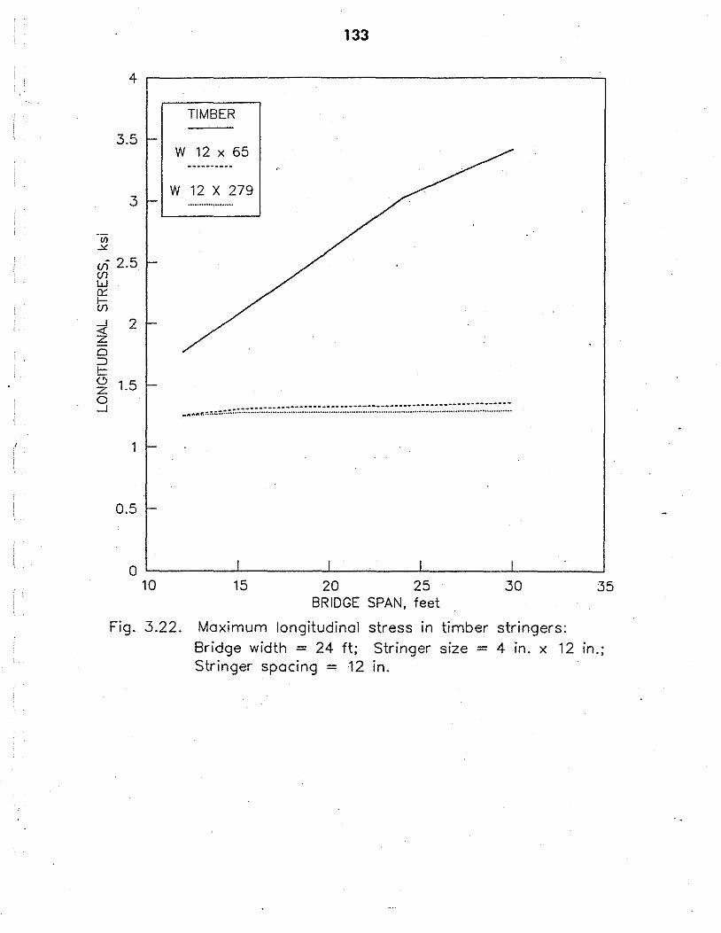
4
3.5
3
vi 2.5 (/) w a:: l!i
~ 0 ::::i I-
2
~ 1.5 0 _J
1
0.5
133
TIMBER
w 12 x 65
w 12 x 279
........ r.l'.:".:".i'.:".:',:'.:'.:'.:'.:'.:'.:".:::::-.:".:.:.:.:.:.:.:.:.:.:.:.:.:::::.:.:.:.:".:.:.:.:.:.:.:.::.::.:.:.~.~-~-~-~-~-~-~-~.~.:=~.~-~-~-~-~-~.
0 '--~~~~'--~~~--..J'--~'--~--'~~~~--'-~~~~-l 10 15 20 25 30 35
BRIDGE SPAN, feet
Fig. 3.22. Maximum longitudinal stress in timber stringers: Bridge width = 24 ft; Stringer size = 4 in. x 12 in.; Stringer spacing -: 12 in.

134
Stringer stresses (timber and steel) are calculated assuming that adequate support to the compression
portion of the stringer has been provided. As the span length increases, different legal loads govern-thus, the
change in slope in the curves shown in Fig. 3.22. Several steel stringers in addition to those illustrated were
investigated, however curves for the other stringers analyzed lie between the two steel curves shown. Thus,
one can conclude within limits the reduction in timber stresses are essentially independent of steel stringer size .
. Stresses in the added steel stringers are obviously a function of steel stringer size. This is illustrated in Fig. 3.23
where the reduction in steel stresses with increased, steel stringer size is shown. This same effect is illustrated
in Fig. 3.24, where steel stringer stresses vs. steel stringer moment of inertias are presented. Additional
computer evaluations verified that stresses in the stei! stringers and timber stringers were essentially
independent of stringer spacings.
The effect of the addition of steel stringers on midspan bridge displacements for one particular situation
is shown in Fig. 3.25. As may be seen, the addition of steel stringers significantly reduces the displacements;
the larger the steel stringers the greater the reduction in displacements.
Figures 3.22 and 3.23 may be used to determine if a given bridge can be strengthened the desired
amount by adding steel stringers. Although these two figures are for one timber stringer size ( 4 in. x 12 in.)
and one stringer spacing (12 in.), it has been shown that this strengthening procedure is essentially independent
of these two variables, and thus these two figures may be used for essentially any practical stringer spacing or
size. Using Fig. 3.22 for a given length of span, one may determine the stress reduction in the timbentringers
resulting from the addition of steel stringers. Entering Fig. 3.23 with the given length of span and limiting
stress, one can determine the size of stringer required. Obviously, stringer sizes other than those shown in Fig.
3.23 may be used if the moment of inertias are essentially the same. Figures 3.22 and 3.23 were developed for
two lane bridges - however, conservatively they may be used for one lane bridges where three steel stringers
are required rather than four.
With the additional steel stringers, load carried by the remaining timber stringers is reduced, since the
added steel stringer carries a larger percentage of the loading. The load carried by the steel stringer is directly
proportional to the stiffness of the stringer (i.e. the stiffer the stringer the more load it carries). Abutments
which were originally designed for essentially uniform loading now need to be reanalyzed and possibly
strengthened to support the reactions from the added steel stringers.
3. 7. Replacement Bridges
This section provides a range of replacement bridges with short span application. While some ·or the
alternatives are technically not bridge structures (e.g. low water stream crossing and corrugated metal pipe
culverts), they serve as means for vehicles to traverse roadway obstacles. Some of the briges presented are
proprietary and information is provided so preliminary decisions can be made regarding potential use of a
particular bridge type. Detailed design procedures and microcomputer design spreadsheets are ~f3vided for
three different timber bridge types. The following sections descnbe each bridge replacement type.
.-·---~. I )
)

135
w 12 x 65
25 w 12 x 120
w 12 x 210
·;;; W 18 X. 2 11 .::L. 20 {/) {/) w 12 x 279 w 0:: I-{/)
_J 15 <( z 0 :::J I-0 z
10 0 _J
5
0 '--~~~~..l.-~~~~-'-~~~~-'-~~~~-'-~~~~--' 10 15 20 25 30 35
BRIDGE SPAN, feet
Fig. 3.23. Maximum longitudinal stress in steel stringers: Bridge width = 24 ft; Stringer size = 4 in. x 12 in.; Stringer spacing = 12 in.

136
30
12' SPAN
25 15' SPAN
18' SPAN
Ill 20 .::<:
24' SPAN
(/) (/) 30' SPAN w 0:: I-(/)
....l 15 <i: z 0 ::i I-(.'.) z 0 10 ....l
5
0 '--~~~~-'-~~~~-'-~~~~-'-~~~~--''--~~~---' 0 1000 2000 3000 4000 5000
MOMENT OF INERTIA OF STEEL STRINGERS, inch~4
Fig. 3.24. Maximum longitudinal stress in steel stringers: Bridge width = 24 ft;· Stringer size = 4 in. x 12 1n.; Stringer spacing = 12 in.

137
01--~~~~/~··.,.......~~--..~--~~~--~--~--~---=--=--=--=--=--~--~-~...,,,.=-~~~~~~-l .. ···•. . .. ····~··· .................................... .
rn <IJ
..i:: v c ·- -2 (/) 1---z w :2 w u <( -4 _J
0... (/)
0
-6
,: ·~.~..... . --.. . .... · /
//, .. >'' .... ,'
/ . // .//
. . . . . .
TIMBER
w 12 x 65
w 12 x 279
-8'--~~~-'-~~~--'~~~~-'-~~~--'-~~~~..._~~~......J
0 5 10 15 20 25
DISTANCE FROM LEFT EDGE OF BRIDGE, feet Fig. 3.25. Displacements in timber and steel stringers:
Bridge width = 24 ft; Stringer spacing = 12 in.; Bridge span = 18 ft; Stringer size = 4 in. x 12 in.
30
138
3.7.1. Precast Cu:trert/Bridge
The Con-Span precast culvert system is a proprietary system licensed by the Om-Span culvert company
of Dayton, OH.
3.7.I.I. Background
The Con-Span precast culvert system was specifically developed to provide a large hydraulic cross.section
with a limited vertical clearance. These precast culvert sections are available in 4 span lengths: 16 ft, 20 ft, 24
ft and 36 ft and in rises from S ft to 10 ft. If these span lengths are insufficient to meet the needs of a
particular location, multiple opening arrangements may be usiid. Figure 3.26 illustrates the Con-Span culvert system. The areh-box shape allows the culvert to carry more
load than an ordinary reinforced concrete box culvert. When the culvert deflects, thrust is developed by the
passive earth pressure or the backfill, thus resisting deflection of the arch top. The culvert cannot collapse
without displacing the block of soil behind the sidewalls a sufficient amount to allow the arch to collapse.
In load tests; the culvert supported a load nearly twice the specified design load of 35 kips (HS-20 loading).
The results of the load test demonstrated the amount of reserve load-carrying capacity present in the Con-Span
system.
Although each installation has site specific details, the procedure for installing a Con-Span culvert is:
• Pour strip footings to support precast units.
• Set precast Con-Span units in place on footings in a bed of cement grout.
• Install engineering fabric over joints to prevent the intrusion of any backfill
• Bolt units together with simple joint connectors on vertical sides.
• Install piecast wingwall (if desired).
One advantage of the Con-Span system is the availability of precast headwalls and wingwalls. These
eliminate the use of time-consuming cast-in-place operations. The headwalls are monolithic with the archbox
end units, while the wingwalls are bolted on after the units are set in place.
3.7.1.2. Design criteria
All Con-Span culvert units are designed to meet AASHTO HS-20 loading criteria. It is possible,
however, to design the culverts to carry essentially any loading. The actual structural design work is performed
by Con-Span engineers in Dayton, Ohio. Engineers desiring to use the Con-Span system simply supply the
desired span length, height of rise, and depth of cover at the particular site location, along with the desired
design load. Con-Span has established a telephone facsimile station to provide rapid preliminary designs. Con
Span engineers provide a preliminary design within 1 hr. after receiving the necessary information.
3.7.1.3. Design requirements
To compute the required hydraulic capacity for a particular culvert location, Con-Span, Inc. has
developed a series of graphs which assist the engineer in determining the required culvert size. Plots of
headwater depth (ft) vs. discharge (ft3/sec) along with tables of waterway areas for the various span/rise
combinations are available for preliminary calculations.

139
5' - 10' rise
I< 16' - 36' span length >I
Fig. 3.26. Con-Span precast bridge S\')gment.

140
For those engineers who have a microcomputer available, a series of input files for the FHWA HY ..S
culvert analysis microcomputer program have been developed. This program, available from the University
of Florida, automates the FHWA culvert design procedure. The Con.Span input files, along with the HY-8
program, assist the engineer in determining the optimum culvert section for a particular site. To use the
program, basic hydraulic information needs to be provided, such as: culvert inlet conditions, slope of culvert
invert, desired culvert capacity, etc. The HY-8 program also provides a limited amount of hydrograph
generation and other hydrologic computations if no other methods are available.
3.7.1.4. Genera/ cost data
Specific cost information is available for the Con.Span system. In Iowa, the Con.Spansystem is available
from Iowa Concrete Products (West Des Moines, Iowa).
The cost of the Con.Span system can be divided into several parts: substructure costs, cost of precast
units, transporta.tion charges, backfilling, paving, etc.
The cost of substructure work is the most difficult to qnantify accurately. As with any other bridge
replacement option, the required substructure is extremely site-specific. The detailed case studies descn"bed
later provides a general estimate of the substructure cost
The cost of the precast units alone (F.O.B. plant) provided by Iowa Concrete Products is presented in
Table 3.8. In addition to the unit prices shown, a royalty fee of $500 per structure must be paid to Con.Span,
Inc.
Transportation charges from the Hampton plant can be computed from the following:
Loads~ 45,000 lb $2.60/mi (loaded)
< 45,000 lb $2.50/mi (loaded)
In addition, trucks detained at a project site will be billed at a rate of $40.00/hr. after the firSt hour.
Table 3.8. Prices for Con.Span culvert units.
HEIGHT OF RISE Span (ft) add per
5 ft 6 ft 7 ft 8 ft 9 ft 10 ft wingwall
16 $1727 $1818 $1914 $2010 $2106 $2202 $632
20 $1980 $2087 $2193 S2300 $2402 $2508 $643
24 $2252 $2345 $2474 $2584 $2695 $2802 $684
Joint connectors: $40.00/joint

141
3. 7.1.5. Cost Information: Oise Studies
Two detailed case studies from Bremer County and Winnebago County, Iowa are presented as eX<1mples
of Con.Span projects.
The Bremer County project, constructed during the winter of 1988-89, consisted of replacing a quad 4
ft x 6.5 ft x 44 ft laminated wood box culvert with a 20 ft x 9 ft x 64 ft Con.Span culverL County costs for the
project are presented in Table 3.9.
The road was closed for less than 2 weeks for the entire installation project. In addition, by extending
the culvert to a length of 64 ft, the need for guardrails was eliminated. This resulted in a savings of an
additional $10,273 on the project.
The Winnebago County project involved the replacement of an existing timber bridge with a 16 ft x 5
ft x 136 ft Con.Span culverL This particular site was situated on a 45 degree skew, which necessitated a
considerably longer culverL The labor on this project, with the exception of substructure work, which was
completed by a private contractor, was performed by county forces. Costs for the project are presented in
Table 3.10.
As with the Bremer County example, this installation eliminated the guardrails at the site, further
reducing project costs.
3.7 :J.. Air Formed Arch Cu!Ycrt
3. 7.21. Background
A new method of culvert construction has recently been developed. The Air-0-Form process, designed
by Concepts in Concrete, of Norman, OK, uses an inflatable rubber membrane as the inside form for the ·
construction of a reinforced concrete arch culverL The inflatable form can be used to construct numerous
cross-section shapes and can be inflated quickly with a minimum of labor.
The following steps are involved in the installation of an Air-0-Form culvert:
• Place a reinforced concrete slab or footing. .
• Place flexil>le metal straps in the desired shape of the culverL. Inflate the balloon form inside
the' straps.
• Place longitudinal and vertical reinforcing steel
• Adjnst air pressure inside the "balloon• t~ the required pressure.
• Apply 6 in. of shotcrete (in one lift).
• Deflate and remove the membrane after the shotcrete has attained the required strength.
A demonstration project has recently been completed by the Iowa DOT to demonstrate the
construction ofan Air-0-Form culverL The conclusions of the Iowa DOT suggest that the Air-0-Form sy5tem
is better suited for longer and larger diameter culvert applications, where the economics are more favorable
(92).

1.42
Table 3.9. Bremer County Con-Span culvert installation costs.
Item and Description Cost
• labor (all county. employees) $ 5,581
Remove existing pavement
Excavation .
Remove existing wood box culvert
Set and connect Con-span units
Backfill with flowable mortar
•Materials $ 22,352
20 ft x 9 ft ·x 64 ft Con-span units
•Equipment $ 3,282
TOTAL COST WITHOUT WINGWALLS $ 31,215
• labor to place optional wingwalls $ 2,666 .
Form and pour wingwalls
• Materials $ 1,670
Reinforcing steel, ties and concrete .
•Equipment s 410
Air compressor for drilling holes
Generator
TOTAL COST FOR CONCRETE WINGWALLS s 4,746
TOTAL COST OF PROJECT $ 35,%1
3.7.2.2. Cost Information· Oise Study
The Crawford Counly installation of an Air-0-Form culvert was completed in the summer of 1991.
This arch culvert was designed for a 950 acre drainage area; preliminary calculations indicated a required
drainage area of 110 ft2• The culvert was designed for a 52 ft length, with a 9 ft semicircular arch section. The
costs on this project are presented in Table 3.11.
3.7.3. Welded Steel 'I'ruBs Bridge
3.7.3.1. Background
A low volume bridge replacement option which has been used extensively in the eastern U.S. is the
welded steel Warren truSS bridge designed by the U.S./Ohio Bridge Corporation of Cambridge, Ohio (32,54)
shown in Fig. 3.27.
I

143
Welded steel plate gussets Top compression chord
Bottom tension chord
Number of anels varies with len th
Fig. 3.27. U.S. bridge welded steel truss bridge.

144
Table 3.10. Winnebago Couniy Con-Span culvert installation.costs.
Item and Description Item Cost Total Cost
• Labor (county employees) $ 6,217
• Substructure labor - contractor . I. $ 4,419
•Materials $ 64,866
Con-span precast units $ 33,764
3/4 in. aggregate (4576 c.y.) $ 19,449
Concrete (101 c.y.) s 4,924
Backfill aggregate (814 c.y.) $ 3,461
2'h in. aggregate (263 c.y.) $ 1,117
Plastic pipe $ 970
t!yebolts to connect units s 640
Lumber for fonns $ 261
Roofing tar (to seal joints) $ 111
Engineering fabric s 99
F!owable mortar (2 c.y.) $ 70
•Equipment s 5,765
Rent CAT D4 bulldozer s 2,900
Rent crane to set units $ 2,865
• Miscellaneous Expenses $ 4,790
A.C.C. patching $ 4,565
Dust control for detour s 225
TOTAL COST FOR PROJECT s 86,057
The U.S. Bridge is available in span lengths of 40 to 145 ft and is generally designed to carry an HS-20
loading, although it can be fabricated to carry heavier design loadings. The bridge can be shop painted any
color, or is available in A588 weathering steel The U.S. Bridge can be designed to accomodate cast-in-place . .
concrete flooring or a wood plank deck supported liy steel floor beams. The company, however, recommends
the use of a corrugated metal deck with an asphalt riding surface.
The wood plank flooring is usually supplied in either 3 in. x 4 in. or 3 in. x 6 in. nominal sizes. These
planks are placed transversely, with the smaller dimension horU:ontal and parallel with the roadway centerline.
If the deck in a particular bridge is too wide for a plank to span the entire width, splices are permitted. A
siiecial expansion angle has been developed to allow for the thermal expansion of the wood plank flooring.
I I
I

145
Table 3.11. Air-0-Form culvert installation costs.
Item Quantity Cost
Concrete, Footing & Headwall 65.8 c.y. $11,844
Concrete, Arch 36.2 c.y. $24,254
Excavation, Class 10 Channel 300 c.y. $900
Excavation, Class 20 . 480 c.y. $3,360
Granular Material, place only 71 tons $213
Mobilization Lump Sum $2,000
Piling, Steel Sheet 435 s.f. $4,350
Steel, Reinforcing, Footing & Headwall 5,870 lb. $2,348
Steel, Reinforcing, Arch 6,235 lb •. $2,494
TOTAL COST FOR PROJECT $51,763
3.7.3.2. Cost Information - Case Study
Albany County, NY currently has thre.e U.S. Bridge welded steel truss bridges in service. The rapid
installation of the bridge system was a primary reason for using the system. A small crew (5-8 people) were
able to install two welded steel truss bridges in approximately three weeks. Recently, a 47 ft long, 24 ft wide
welded steel truss bridge was installed to replace an existing structure. This installation was designed for HS-20
loading and utilized a wood plank floor system. A summary of the cost of this particular installation is provided
in Table 3.12.
3. 7.4. Prestressed Conaere Beam Bridge
3. 7.4.1. Background
There are numerous examples of precast, pres tressed concrete sections which are suitable for low-volume
bridge replacements. The standard bridge sections which have been developed by the Prestressed Concrete
Institute (PCI) (60) and AASHTO are well-known and have been used extensively throughout the United
States (see Fig. 3.28). The majoricy: of these sections were designed for long-span bridges and so are usually
over-designed for a low volume bridge application. The AASHTO shapes are particularly inefficient, since they
were developed several years ago when full prestressing (no tensile stresses at service load) was considered
essential (55).
In addition, many prestress plants have designed their own non-standard sections. The majority of these
non-standard sections are not patented, so that in most instances another prestress plant can obtain the
necessary dimensions and enter bids on a proposed project One significant benefit of many of these non-

148
Of all the shapes being used, the bulb tee is the most efficient. On the other hand, the double and multi
stemmed tees and the channel sections have the advantage of being more stable during handling and placing,
and therefore are generally preferred by contractors (82). Sections which have nearly vertical flush sides, such
as the box beam, can be connected transversly by bolting through the legs, which eliminates the need for
intermediate diaphragms.
One section which takes advantage of this configuration is the 'OK' bridge system, which was developed
at Oklahoma State University. nm system is discussed in greater detail later in this report (see Sec. 3.7.6).
3. 7.4.2. Design Criteria
The actual design of a prestressed concrete girder bridge is relatively straight-forward. Several references
are available to assist the practicing engineer with the design procedure (62,63). Brief guidelines for the design
of a prestressed concrete double-tee follow. All dimensions and section properties are general values. Because
each prestressed concrete manufacturer provides slightly different products, the exact values may differ slightly.
A design aid has been developed by the PC! to simplify the selection of a prestressed double-tee section.
Table 3.14 provides the section properties for a number of standard size prestressed double-tee girders (see
Figure 3.29).
Table 3.14. Section properties - prestressed double-tee girders.
Dimensions (in.)' WL Area I. s. w D T A c E (lb/Ct) (in') (in') (in')
60 Z7 5 4.50 8.00 36 599 575 33,740 4020 L I 72 23 5 4.50 6.50 36 582 558 21,366 3345 0 H 72 Z7 5 4.50 8.00 36 662 635 . 35,758 4560
T 96 Z7 5 3.75 5.75 48 718 689 32,888 5171
96 35 5 3.75 6.50 48 820 787 72,421 8230
60 36 6 6.00 8.00 30 812 780 90,286 7334
72 35 5 6.00 9.75 48 876 840 90,164 7706
84 35 s 6.00 9.75 48 938 900 95,028 8569
H 96 35 5 6.00 9.75 48 998 960 99,299 9412
E 72 Z7 5 7.00 9.75 48 761 731 45,084 5060 A v 84 Z7 5 7.00 9.75 48 824 791 47~486 5640 y
96 Z7 5 7.00 9.75 48 886 851 49,566 6196
72 21 5 7.75 9.75 48 671 644 22,720 3298
84 21 5 7.75 9.75 48 733 704 23,903 3666
96 21 s 7.75 9.15 48 796 764 24,920 4019
'See Fig. 3.29.
I

149
w
> < l ;
; D ; i ; ; i ' '
E ' 1--i-- ;
! _...
tk _c _ - ,
Fig. 3.29. Standard pres tressed concrete double-tee bridge girder.

150
3. 7.4.3. C-Ost Information: Case Study ·
A 124 ft long by 24 ft wide two-span continuous prestressed concrete double-tee bridge was installed
in Washington County, Iowa in 1988. Costs incurred by the county are presented in Table 3.15.
3. 7.5. Inverset Bridge System
3.7.5.1. Background
A unique method of utilizing !he best features of both steel and concrete has been developed by
Grossman and Keith Engineering of Norman, OK. The Inverset bridge (see Fig. 3.30) is a proprietary system
which is cast upside down to utilize !he compressive strength of concrete and !he tensile strength of structural
steeL
Table 3.15. Prestressed double-tee beam installation costs.
Item Description Amount Cost
Concrete, Structural 143.2 c.y. $14,833
Reinforcing steel 27,133 lbs. $6,783
Prestressed Concrete Double Tee 6only $27,000 56 ft. 414 in.
Prestressed Concrete Double '.I'ee 6only $31,500 67 ft. 414 in.
Steel piling HP10x42 • furnish 1305 Lf. $15,660
Steel piling HP10x42 • drive 1305 Lf. $3,263
Steel piling HP10x42 • encase 159.4 Lf. $4,782
Excavation, Class 20 8S c.y. $680
Excavation, Class 21 16 c.y. $320
Excavation, Class 10, channel 951 c.y. $1,902
Rail, concrete barrier 284 Lf. $4,260
Removal of existing structurell? lump sum $5,000
Mobilization lump sum $3,000
TOTAL COST FOR PROJECT $118,983
COST PER SQUARE FOOT S39.98/ft2
In precasting, !he forms are suspended from steel beams. In !his configuration, the weight of the forms,
steel W sections, and wet concrete places compressive stress in what would be the bottom flange when !he unit
is inverted. When !he concrete cures, !he units are turned 'rigbtside-up'. The casting procedure results in !he
,.,, ..... ...._ ;
I ·'

END SUPPORTS
151
:ROLLED BEAM WITH SHEAR CONNECTORS
L---TRANSVERSE FORM SUPPORT
END SUPPO:RTS
Fig. 3.30. lnverset bridge section during fabrication.

152
bottom flange having essentially zero stress. This stress condition, combined with the increa5ed moment of
inertia of a composite section, allows the lnverset system to carry additional load without overstress.
When the unit in turned over, longitudinal compressive stress is applied to the slab, which makes the
deck extremely crack resistant and impervious to water intrusion (because air bubbles formed on what will
eventually be the bottom of the slab).
3. 7.5.2. Example
A sample Inverset design and fabrication is descnoed in the following paragraphs. Particular attention
should be paid to the stresses in the steel and concrete during the various steps of fabrication. In the example,
stresses will be computed at the following locations in the cross-section:
• Concrete - extreme compression fiber of the deck,
• Steel - top flange of steel girder (which contains shear connectors) when the unit is placed into
service, and
• Steel - bottom flange .of steel girder once unit is erected. This flange is in compression
during fabrication and is in tension when in service.
A summary Of the stresses at various stages of the life of an Inverset bridge section are presented in
Table3.17.
1. Dcaign aflcria.
Simply supported span = 34 ft
Width of one unit, W = 11.833 ft
Design live load: AAsHrO HS-25
Steel girder: W24x55 ASTM A572 grade 50
Yield strength = 50 ksi
Section modulus = 114.S in.3
Form weight = 100 lbs/ft
Concrete strength, f.' = 5 ksi
The allowable stresses in steel and concrete are:
Temporary stresses (~art 9.15.1, AASHrO (2)):
Steel:
tension: 0.80 F, = (0.8)(50) = 40 ksi
compression: 0.70 F, = (0.7)(50) = 35 ksi
Final stresses:
Steel (See 10.32.lA, AASHrO):
tension: 0.55 F1 = (0.55)(50) = 27 ksi
compression: 0.55 F1 = (0.55)(50) = 27 ksi
i J·

153
Concrete (See art. 8.15.2.1, AASHTO):
f., = 0.40 f.,' = (0.40)(5) = 2 ksi
2. Slleasca due to beam weight.
M = wl2 = (2)(55 lb/ft)(34/t)2 = 15.90 ft-k 8 (8)(1 OOOlb/k)
lb = M = (15.90ftk)(12in/ft) = O.B3 ksi T S (2 beams)(114.5in3) c
3. Stresses due to furm weight.
M = w/2 = (100 lb{ft)(34/t)2 = 14.45ft-k 8 (8)(1 OOOlb/k)
top bott.
fb = M = (14.45.ftk)(12in/ft) = 0.76 ksi T S (2 beams)(114.5in3) c ~~tt.
• 4. Stresses due to weight of conaete.
w = (7.50 in.)(11.833.ft)(150 lbfft3) = 1109 lb{ft 12 in.lft
M = w/2 = (1109 lb{ft)(34/t)2 = 160.26.ft-k 8 (8)(1 OOOlb/k) ·
f, = M = (160.26 ftk)(12infft! = 8.40 ksi T top b S (2 beams)(114.5in3) C bott
At this stage, the stress in the top and bottom flange can be expressed by:
f..,. = 0.83 + 0.76 + 8.40 = 9.99 ksi T
r ... = o.83 + 0.16 + 8.40 = 9.99 ksi c
S. Computation of composite section propertlca. When the concrete has attained a strength of
2.00 ksi, the forms can be stripped. At this point, a composite member has been developed.
The section modulus of the composite member is calculated by the transformed area method.
The modular ratio, n, is taken as 7 for strength Calculations and as (3 x 7) = 21 for creep
effects.
(See Section 10.38.1, AASHTO (2)).
For n = 7:

154
I = 9,508.48 in', N.A located @ 24.23 in.
(Note: N.A is located 0.66 in. above top flange)
For n = 21: I = 7,516.02 in', N.A located @ 21.06 in.
Note: N.A is located within the steel girder.
A summary of section moduli for composite Inverset sectiqns is presented in Table 3.16.
Table 3.16. Section moduli for composite Inverset sections.
Section Moduli for Composite Members (in.))
Location n=7 n = 21
Concrete (top of deck) 1,389.84 750.83
Steel girder (top flange) 14,137 2994.1
Steel girder (bottom flange) 392.45 356.89
· 6. Rcmaval of forms. When the forms are removed, the load acting on the composite section is
reduced. This reduced load reduces the stresses in the steel girders, and the concrete deck
becomes prestressed. The bending moment caused by the weight of the forms is the same as
computed earlier, M = 14.45 ftlc.
The stress in the concrete, t,._:
f. = M = (l4.4Sftk)(12inffr) = 0.011 ksi C """" s (21 )(750.83in3>
The stress in the top flange, i;.,.:
f. = M = (14.45.ftk)(12in[fr) = 0.06 ksi ,,. s 2994.1 in3
c
The stress in the bottom flange, C,,..:
' Ji = M = (14.45.ftk)(12 inf/!) = 0.49 ksi T bot s 356.89 in3
7. Ullill turned to upr:i&ht posllion. When the units are turned over to their upright position, the
forces acting on the units are essentially reversed. The process of inverting the unit causes a
change in stresses equal to twice the weight of the structure. The moment due to overturning
of units can be computed as:
M = 2(15.89 ft-k + 160.25 ft-k) = 352.29 ft-k.
The stress in the concrete, r,._:

155
/, = M = (352.29ftk)(12in/fi} = 0.268 k.si """' S (21 }(750.83in3)
c
The stress in the top flange, r,,,,:
J. = M = (352.29 ftk)(12in/fi} = 1.41 k.si C .,,, s 2994.1 in3 .
The stress in the bottom flange, f..,.:
f, = M = (352.29 ftk}(12 in/Ii) = 11 •85 k.si T ""' S · 356.89 in3
8. Application of auperimpoeed dead loads. Superimposed dead loads are assumed to act
uniformly over the bridge deck surface. Superimposed dead loads include such things as: curbs,
utility lines, guardrails, and parapets or other additional weights. For purposes of design, the
dead load of any future wearing course should be included in the superimposed dead load. For
this example, assume a or..,,... = 65 lb/ft2•
So, w.,.., = (65 lb/ft2)(11.83 ft wide) = 769.0 lb/ft
The moment due to this DL..,., is:
M = wl2
= (769.0 Uffe}(34ft}2
= 111.1 ft-k 8 (8)(1 OOOlb/k} . .
The stress in the concrete, C...,.:
/, = M = (111.1ftk)(12in//i} = 0.085 k.si C """' S (21}(750.83in3)
The stress in the top flange, f,,,.:
J. = M = (111.1 ftk)(12in//i} = 0.4S k.si C ""' S 2994.1 in3
The stress in the bottom flange, t;,..:
f, = M = (111.1ftk}(12in//i} = 3.74 k.si T ""' s 356.89 in3
9. Application of AASHTO design li'le load. For this example, an HS-25 loading will be used.
The maximum live load moment for a 34 ft span is 429.4 ft-k (see Appendix A, AASHTO
Standard Specifications (2)). This design live loading must be adjusted for the wheel load
distnoution width and impact to determine the actual design moment.

156
The wheel load fraction can be calculated from 3.23.1, AASHTO, with the beam spacing taken
as one-half of the width of the Inverset unit (See design criteria).
WLF = __§__ = W'ulth of unit = 11.83ft = 1•076 5.5 (2)(5.5) (2)(5.5)
The impact factor (See Article 3.8, AASHTO) can be eomputed as:
50 50 I= 1 + L + 125 = 1 + 34 + 125 = 1.315
I= 1.315 ~ 1.300(max.) :. I= 1.300
The design live load moment, Mu, is computed by:
Mu= M x WLFxl =(429.4ft-k)(1.076)(1.300) = 600.51 ft-k
The stresses due to the live load moment must be computed with the modular ratio = 7. This
increases the effective section modulus of each element of the composite member.
The stress in the concrete; r.,,..;
/. = M = (600.5ft-k)(12in/ft) = 0.741 ksi C """" S (7)(1389.84in3)
The stress in the top flange, t;.,.:
frop = M = (600.5 .f!-k)(12in/ft) = 0.51 ksi T s 14,137 in3
The stress in the bottom flange, f ... :
Ii = M = (600.5ft-k)(12 in/ft) = 18.38 ksi T bot S 392.45 tn3
This example problem illustrates that at no time during fabrication, installation, or service load conditions
does the Inverset cross section exceed the allowable stress and that at final service load conditions, a
compressive stress of 1.105 ksi exists in the concrete. This final compressive stress serves to reduce deck
cracking and the intruSion of water. ·
Load transfer between adjacent units is provided by steel diaphragms which are bolted in place
after the units are set in place. The longitudinal joints are sealed with a non-shrink grout in conjunction
with an elastomeric concrete sealer (see Fig. 3.31).
The technij ue of casting Inverse! bridge decks upside down allows the manufacturer to incorporate
a number of deck finishes at minimal additional cost If the desired finish is smooth (as when a waterproof
membrane and asphalt overlay are used), the concrete bed is constructed with smooth finished plywood. If
' ..... ~ .

157
·- .. -~.·
Asphalt overlay~~~
Waterproof membrane
Backer rod _J
a. with overlay
Non-shrink grout Elastomeric concrete
Backer rod _J
b. without overlay
Fig. 3.31. Longitudinal joint details for lnverset bridge.

158
a textured wearing surface is desired, a urethane form liner is included before the concrete is placed. A
natural finish may be achieved by using the standard coarse sandblast form liner and sawing transverse
grooves after deck erection at an estimated cost of $0.50/ft2• For additional information on the Inverse!
system, the reader is directed to Ref. 31.
Table 3.17. Inverse! bridge section stresses over life of bridge.
Stresses in various elements of composite section due to fabrication and service loads
Bottom Flange Top Flange Concrete
Load Stress Total Stress Total Stress Total (ksi) (ksi) (ksi) (ksi) (ksi) (ksi)
Beam 0.83 c 0.83T Weight
Form 1.59 c 1.59 T Weight
Concrete 9.99C 9.99T
Remove 9.50 c 9.93 T 0.011 c forms
Invert 2.35 T 8.52 T 0.279 c Super. 6.09T 8.07T 0.364 c DL .
Live 18.36 T 24.45 T 0.51 T 8.58T 0.741 c 1.105 c Load .
3. 7.5.3. Cost Information: Case Study
A series of case studies are provided for the Inverse! bridge system. Several of the Inverset bridges
have been installed in the state of Texas as complete design-b.uild, or turnkey, projects. Cost information
for these projects have been provided by Steele Construction Company. The costs for these projects
includes the following items:
• Royalty fee paid to the designer
• Engineering with stamped plans
• Demolition of existing bridge
• Pile driving (using 16 in; square precast concrete piles)
• Pile caps
• Deck
• Guardrail
!
)

159
• Embankment at ends of bridge (no deck overlay)
• Bonding
In addition, similar components have been utilized for all bridges:
• 3 pile bents
• Pile caps: 2 ft-3 in. x 2 ft x 28 ft
• Abutments: 2 ft-3 in. x 2 ft x 28 ft (with backwall)
• 7 in. concrete deck
• Type T-6 guardrail with safety end treatments
A summary of the project costs is presented in Table 3.18.
Table 3.18. Inverset bridge installation costs.
Span Project Name Lengths
Whipporwill Road 3x30'-0"
Stidham Road 30' -40'-30'
Nichol Road 4 x 42'-10"
Walnut Creek Road 4 x 37'-10"
Uncle Glen Road 4 x 45'-3'
Humble Pie Rd. 2 x 45•.g•
Brazos River 10 x 40'-0"
3.7.6. Precaat Multiple Tee Beam Bridge
3.7.6.1. Background
.
Bridge Width
26'-1'
26'-1'
26'-1"
26'-1"
18'-1'
28'-1'
16'-0'
Pile Length
(ft)
40
40
45
45
50
35
25
Project Cost Cost ($/ft') ($)
79,730 33.96
88,589 33.96
150,961 33.78
148,775 37.69
147,000 44.91
85,900 31.43
201,253 31.44
A non-prestressed double tee beam girders has been developed by the Oklahoma State University
Center for Local Technology which can be fabricated by local crews during the slack time of the year. The
"OK' girders can be fabricated with reuseable steel forms that county crews can construct from standard
structural shapes. This system offers a significant reduction in material costs and construction time over
comparable alternatives. Oklahoma State University believes that the design can provide savings of •at
least 15 perce.nt• over conventional designs.
The "OK" bridge girder is a modified double tee reinforced concrete beam 17 in. deep by 41'h in.
wide (see Fig. 3.32) which can carry an HS-20 loading over spans of 20-25 ft. The beams are bolted
together at third points with 1 in. diameter threaded rods to form various widths; seven of the units bolted
together will provide a width of 24 ft - 2Vi in. The shear key at the top corners of each girder provides for

/ /
I ,
160
'( -----.,..,,,.. ....... : ,,,,,,. ... I ,;' I I I I
~---l
Adjacent precast sections
41 1/2"
17"
15"
~-
Typical section view
Fig. 3.32. "OK" precast mu!tip!e tee beam section.

161
shear transfer, and when filled with a non-shrink grout, prevents independent movement of adjacent
girders. The two exterior girders are desigiied with connections for guardrail
Each "OK" bridge girder weighs 5.67 tons and contains 2.6 cu. yd. of 3500 psi concrete. The top face
of the girder is rough-finished providing ready-made wea~g surface, although the design provides for a 20
psf wearing surface.
Several counties in Indiana have been using the 'OK' bridge system for the past two years and report
great success. The Daviess County, Indiana Highway Supervisor estimates the design will save the county a
half-million dollars in the next 10 years (17). For additional information on the 'OK' bridge girder system,
see Refs. ( 46,65).
3.7.6.2. Cost Information: Case Study
The cost information for the 'OK' girder has been well documented by Daviess County officials. The
cost of the project, including one-time expenses such as the concrete pads, rebar jigs and forming are
shown in Table 3.19.
3.7.7. Low Water Stream Crossing
3.7.7.1. Background
One relatively low-cost bridge replacement option available to the county engineer is the Low Water
Stream Crossing (L WSC). A LWSC is defined as a stream crossing structure that is designed and
constructed so that it is overtopped by floods or high water several times a year (49).
Since a LWSC is a low structure with a simple substructure, it is relatively inexpensive to construct.
Unfortunately, since it is overtopped by high water several times per year, a LWSC creates regular traffic
detours and inconveniences. In addition, the damage caused by high water erosion necessitates frequent
inspection and inexpensive repair. These features may make a LWSC an economical replacement structure
for low volume rural roads especially in areas with broad floodplains or where the normal streamflow is
quite shallow.
Listed below in decreasing order of complexity and expense are three types of lowwater stream
crossings:
• Low water bridge,
• Vented ford (a dip with vent or drain pipes},
• Simple ford or dip.
A low water bridge can be constructed by lowering the vertical alignment of the approaching
roadway and constructing the bridge deck so normal stream flow can pass beneath. A low water bridge is
especially suitable in areas where the potential excessive debris exists or where environmental conditions do
not allow alterations of the existing streambed.
A vented ford is a dip in the existing roadway grade with pipes installed under the roadway to allow
for day-to-day streamflow. A vented ford is the generally preferred alternative when the normal depth of
the stream exceeds 4 to 6 in.

162
Table 3.19. "OK" multiple-tee beam bridge girder project costs.
Item or Description Cost
Pour 40' x 14' x 6" concrete pad:
Concrete (13.25 c.y., 3500 psi) s 563.13 ' I ., Trowel machine rental s 30.00 '
Anchor bolts, assorted hardware s 38.58
Reinforcing steel . s 146.00
Labor ( 4 men, 1 day) $ 300.00
TOTAL COST FOR PAD s 1,071.71
Build steel form and rebar :
Materials s 1,795.67
Machine shop (cut, drill, weld steel) s 99.00
Labor (80 hours - form, 40 hours • place steel) s 1,125.00
TOTAL COST FOR FORM AND REBAR s 3,019.67
TOTAL ONE-TIME COSTS FOR 'OK' SYSTEM s 4,091.38
Pour interior bridge beam (5 per bridge):
Reinforcing steel s 243.36
Concrete (2. 75 c. y., 4000 psi) . $ 129.25
Miscellaneous materials $ 6.79
Contract labor to form rebar $ 49.00
Labor to build rebar cage (2 men, 2 hours) s 40.00
Labor to pour (4 men, 1 hour) s 40.00 .
TOTAL COST FOR INTERIOR BEAM s 508.40
Pour exterior girder (2 per bridge):
Same materials/labor as for exterior beam $ 508.40
Exterior bearing plates (4 per beam) s 16.56
Reinforcing steel $ 2.00 . TOTAL COST FOR EXTERIOR BEAM s 526.96
Materials to bolt beams together s 185.00
TOTAL COST FOR ONE BRIDGE DECK s 3,780.92
1.

163
A simple ford is constucted by lowering the approach grades to the steambed level and providing
some sort of unsurfaced crossing. Numerous improvements can be made to this arrangement by providing
an ACC or PCC paved crossing or building some type of end walls. It is recommended that the. user place
reflective markers to delineate the edges of the improved crossing.
3. 7. 7.2. Design Criteria
A risk-based design approach has been suggested for the selection of LWSC locations.
Unfortunately, a detailed risk analysis would require a significant amount of case study data which has not
yet been compiled. A simplified selection criteria was developed in Rel 49 and is shown in Table 3.20.
The possibility of loss of human life criteria noted in Table 3.20 is the most difficult to quantify and is also
the most important criteria for a public works project.
Table 3.20. Low water stream crossing selection criteria.
Most Favorable Least Favorable Criteria forLWSC forLWSC
.
Average Daily Traffic < Sv.p.d. > 200v.p.d.
Avg. Annual Flooding < twice/year >10/year
Average duration of traffic interruption during high water < 24 hours > 3 days
Extra travel time for detour . < 1 hour > 2 hours
Possibility of danger to .human life < 1 : 1 billion > 1: 100,000
Possible amount of property none $1 million damage
3.7.7.3. Cost Information: _Cast Study
Three low water stream crossings have been installed in Lucas County, Iowa in the past five years. A
case study is presented for each of these structures. Labor on all three of the projects includes the removal
of the existing thru-truss bridge at the site and the installation of the low water stream crossing.
The first installation was over the Chariton River in 1987. The structure is a simple vented ford, with four
CMP pipes placed under the crossing. A summary of the costs on this project are shown in Table 3.21.
The second installation was placed over the South Otter Creek in 1987. This structure was another
vented ford, with nine CMP culverts to allow stream flow beneath the structure. Costs on the project are
shown in Table 3.22.

164
Table 3.21. Low water stream crossing costs - Example 1.
I Item and Description I • Labor (county employees)
•Equipment
•Materials
·Rip rap
28 - 20 ft sheet pile
Concrete (29.S c.y.)
4-18in.x28ftCMP
Sand (90.13 tons) ·
Reinforcing steel
Welding supplies
Engineering fabric
TOTAL COST FOR PROJECT
Table 3.22. Low water stream crossing costs - Example 2.
Item and Description
• Labor (county employees)
•Equipment
•Materials
Rip rap & road stone ( + haul)
64 - 18 in. x 10 ft sheet piling
Concrete (46 c.y.)
9-18 in.x30 ft CMP
Sand (125.16 T + haµling)
Lumber for formwork
Reinforcing steel (1,030 lb.)
Engineering fabric (128 c.y.)
Welding supplies
TOTAL COST FOR PROJECT
Item Cost
$ 2,690.65
$ 2,618.00
$ 1,519.25
s 944.48
s 216.31
s 107.92
s 31.68
s 22.63
Item Cost
$ 5,648.70
s 2,992.00
$ 2,369.00
s 2,250.00
s 738.45
s 205.13
$ .185.40
s 122.64
s 29.63
I Cost
s 3,062.41
s 4,485.96
s 8,150.92
s 15,699.29
Cost
s 4,231.51 ·
s 3,328.50
s 14,540.95
s 22,100.96
I ,,.,.--..., \ )
.... ,.
i

165
The third installation was over the Wolf Creek in 1989. This installation included a skewed arrangement
of seven CMP under the roadway surface. Costs on this installation are presented in Table 3.23.
Table 3.23. Low water stream crossing costs - Example 3.
Item and Description
• Labor (county employees)
•Equipment
•Materials
Rip rap & hauling
80 - 18 in. x 10 ft sheet piling
Sand (incl hauling)
Concrete (29.8 c.y.)
7-18in.x32ftCMP
Reinforcing steel (812 lb.)
Engineering fabric (128 c.y.)
Lumber for formwork
TOTAL COST FOR PROJECT
3.7.8. Corrugated Metal Pipe CuM:rt
3.7.8.1. Background
Item Cost Cost
$ 4,131.67
$ 2,729.00
$ 14,652.10
$ 3,862.21
s 3,700.00
$ 2,815.79
s 2,079.00
$ 1,847.16
$ 273.78
$ 122.64
$ 74.16
$ 21,572.77
A corrugated metal pipe culvert (CMP) offers many advantages over other bridge replacement
alternatives. A CMP is faster and easier to install than a cast-in-place concrete structure. In addition, there
are no forms to set and remove, and no curing time is required. In most cases, county forces can install a CMP
using ordinary county-owned equipment, which eliminates the need to hire an expensive outside crew or rent
equipment To simplify design, numerous standard CMP sections have been developed. These standard
sections are mass produced which lowers the material costs.
There are actually several types of CMP culverts available. Many of these have been available for years,
and have proven to be a cost-effective bridge replacement alternative. This report will concentrate on one
particular type of CMP, the corrugated aluminum box culvert Although only one type will be discussed in . .
detail, many of the same considerations can be applied to corrugated steel pipes, and other CMP culverts.
Much of the information printed in this report was developed with the assistance of Contech Construction
Products, Inc. Although the culvert dimensions and available accessories discussed are specific to Contech

166
there are other CMP manufactures which produce similar CMP. The design and installation procedure is
similar for each of the different brands of CMP culverts, thus generalized instructions are presented.
The CMP culvert which offers the best potential for low volume bridge replacement is the aluminum
structural plate box culvert. Corrugated aluminum box culverts (CABq combine the low profile shape of rigid
box culverts with the strength and fieXll>ility of fieXll>le structures. Contech Aluminum Box Culverts are
available in standard sizes ranging from 8 ft-9 in. x 2 ft-6 in. to 25 ft-5 in. x 10 ft-2 in. The box culvert consists
of aluminum structural plates and reinforcing nos which are curved and bolt-hole punched at the plant.
One advantage the CABC has over other culvert types is the corrosion resistance. The aluminum alloys
in the structural plates have an excellent resistance to corrosion, due to a thin oxide layer which forms on the
metal surface when exposed to air. Many agencies are predicting a service life of more than 50 years for 16
gauge aluminum culverts when subjected to a normal environment. To minimize corrosion in the system, no
dissimilar metals should be allowed to come in contact with the culvert. Although galvanized fasteners are
acceptable, other metals must be insulated with non-conductive coatings.
One of the main advantages of an aluminum culvert system is its lightweight. Aluminum structural plate
weights approximately 2 percent of a similar size reinforced concrete pipe. This lower weight reduces assembly
and equipment costs and facilitates easier handling of the larger sections. The aluminum structural plates are
usually light enough to be handled by a single worker, thus reducing labor costs. In addition~ it is possible to
assemble the culvert offsite and place it with smaller lifting equipment. This saves the cost of a heavy duty
crane, and reduces the time the site needs to be closed for construction. All of these advantages make it
possible to re-open the road more quickly, V.:hich reduces the inconvenience to the public.
3. 7.8.2. Design Criteria
All Contech Aluminum Box Culverts are designed to meet or exceed an AASHTO HS-20 live loading.
The actual structural design is performed at the Contech headquarters in Middletown, OH, and utilizes a finite
element procedure to calculate the culvert load-carrying capacity.
The practicing engineer is required to perform the hydraulic design for the proposed culvert location.
In following section, information on the hydraulic design of a CABC is presented. The footings used by a
CABC require that the foundation soil be able to support a bearing stress of at least 4000 lb/sq ft. Existing
foundation materials which are unable to support a load of this magnitude should be replaced before installing
a CABC.
To retain the culvert's design load carrying capacity, the proper amount <)f earth cover must be
maintained above the culvert. Contech recommends that the roadway above the structure be designed with
either a fleXJl>le or rigid pavement. The minimum amount of cover Jitustbe maintained to prevent high-impact
loads from being applied to the culvert. Particular attention should be paid to the shoulder of the prop<ised
roadway, where a combination of substandard cover and an applied wheel loading can damage the culvert.
" }
I I
.1

r '-
167
3. 7.8.3. Design inform a lion
The actual hydraulic design of a CMP culvert is beyond the scope of this project. There are however,
a number of sources available which d~ the hydraulic design procedure in detail The reader is particularly
encouraged to review the AISI Steel Drainage Handbook. The engineer should be aware of several optional
design features of CABC.
Several types of footings are available for corrugated aluminum box culverts. A corrugated aluminum
invert can be supplied for those installations which do not merit a full paved invert. The engineers at Contech
strongly recommend that steps be taken to avoid water intrusion under the invert. Intrusion may be prevented
by installing a toewall on the upstream end of the culvert. A concrete toewall may be cast on-site, or an
aluminum flat sheet toewall is available. Note that most short-span culverts are goverened by inlet controL
In such cases, the roughness coefficient of the invert does not affect the hydraulic capacity of the culvert, and
the corrugated invert is often the most economical footing available.
In those l0cations where a full corrugated invert is used, it is essential that no backtill material intrude
through the corrugations at the sidewall-invert interface. A scalloped closure plate is available to minimize the
amount of this backfill infiltration. If the backfill material contains a significant amount of fine silts or sands,
a layer of geotextile should be installed along the joint as welL
A pad footing is available for sites where the stream bed consists of non-erodible material; these are
generally more economical than a full invert A pad footing should be buried to a minimum depth of 12 in.
to allow the inside soil to balance the pressure due to backfilling. It should be noted that the flow area of a
box culvert includes the area from the crown to the invert or footing pads. If the pads are buried, the
reduction in hydraulic capacity must be considered.
CABC's arrive at the jobsite ready for assembling. The parts are numbered and lettered for ease of
erection. No unusual tools are required for assembly; drift pins and an impact wrench with a capacity of 150
ft-lbs. are considered mandatory. The keys to efficient assembly of the culvert are the use of a pair of drift
pins to align the holes and proper bolt sequencing.
Site preparation, excavation, bedding, and backfill operations are essential to develop the maximum
strength of any flexible culvert The soil around the culvert must be sound granular material, placed and
compacted following accepted procedures. The following remarks are specifically directed toward a CABC
installation, but can be generalized to other types of culverts as welL
If a full aluminum invert is used, the trench bottom must be equal to the span of the culvert plus
sufficient room to allow proper compaction. The bedding directly beneath the culvert sidewalls is particularly
importanL This region must receive proper compaction to develop the maximum load carrying capacity of the
culvert When toewalls are added, whether concrete or aluminum, a crosstrench must be included across the
full width of the invert.

168
Installations utilizing aluminum foot pads require the excavation of two trenches. These must be of
sufficient width to install the pads, .and mpst be deep enough to avoid possible scour and frost heave of the /
pads. .
The preparation of the pipe bedding is critical to both culvert performance and service life. Avoid any
distortions that may create stress concentrations in the culvert. The bedding material must be free of rocks,
frozen material, and organic material that might cause unequal settlement. Contech recommends that the
bedding material be a well graded granular material
The proper placement and compaction of backfill material is essential to developing the maximum
strength of the culvert. The same basic restrictions apply to the backfill as to the bedding material One
should avoid anything which might create uneven compaction. The backfill material must be placed
symmetrically on each side of the structure in 6-8 in. lifts. Each lift should be compacted to a minimum of 90
percent maximum density before applying more backfill material During the backfilling operation, only small
tracked vehicles should be near the culvert. If larger vehicles must be used, it may be necessary to increase
the minimum cover depth to carry the temporary loading.
3.7.8.4. General cost infonnation
A double 21 ft-2 in. by 8 ft-10 in. x 64 ft Con-Tech Corrugated Aluminum Box Culvert was installed by
the city of Galesburg, IL in the summer of 1991. The existing timber bridge had to be removed and replaced
after fire caused major damage to the deck and timber pile abutments ..
The labor on the project was performed by a city maintenance crew, with the exception of the the
removal and disposal of the existing creosote-treated bridge deck. Costs for th!l project are presented in Table
3.24.
3.73. S1reas-I amlnated Timber Bridge
3. 7.9.1. Background
The stress-laminated timber (stresslam) system is a relatively new concept for timber bridge construction.
In this system, sawn lumber laminations are placed vertically and squeezed or clamped together on their wide
faces by the use of high strength steel post-tensioning rods. A stresslam bridge offeis several significant
advantages over conventional nail-laminated timber bridge systems. The deck supeistructure can be
prefabricated into panels, which can then be transported to the site and lifted into place. As long as the post
tensioning force is properly maintained, the stresslam timber deck will not delaminate over time. In the
stresslam system, it is not necessary to have individual laminates span the entire length of the bridge: Since
the load transfer between laminates is entirely by friction at the interface, all laminations do not need to be
continuous. Butt joints of individual laminates are permitted within certain limitations (usually no more than
1 butt joint in 4 laminations within any 4 ft segment of deck width). The forces in a discontinuous lamina at
..... ,.,

'· '• - .
169
Table 3.24. Corrugated aluminum box culvert installation costs.
'
Item and Description Item Cost Total Cost
• Labor (city employees) $ 8,410
• Removal of existing ' $ 8,000
structure (contractor)
• Materials $ 42,294
Aluminum box sections $ 24,450
3/4• Aggregate (2875 c.y.) $ 12,219
Concrete (62 c.y.) $ 4,650
Miscellaneous materials $ 975
• Heavy Equipment Rental s 4,500
• AC.C. wearing surface $ 1,688
TOTAL COST FOR PROJECT '
$ 64,892
a bun joint are transferred to tbe adjacent lamina tbrough friction, which carry tbe forces past tbe butt joint
(57). This behavior allows the use of shorter lumber and also allows longer spans to be Cambered to offset
dead load deflections.
The stress-laminated timber bridge system was developed by tb.e Ontario (Canada) Mininstry of
Transportation and Communication (Ontario M.O.T.C.) in tbe mid-1970s as a metbod of rehabilitating existing
nail-laminted bridges (80). Traffic loading had caused timber deck members to separate, reducing tbe load
distribution ability of tbe bridge deck and causing severe deterioration of tbe asphalt wearing surface. As
shown in Fig. 3.33, tbe original techni{ ue used steel prestressing rods placed above and below tbe existing deck,
which were tben tensioned to compress tbe deck. The effects of tbe stress-laminating were dramatic and
substantially increased tbe load-carrying capacity of tbe bridge (81).
Based on tbe successful application of tbis procedure to existing bridges, a method for constructing new
bridges witb a stresslam deck was developed. The system for new construction is similar to the original system,
except tbat tbe prestressing rods are placed in transverse holes in tbe laminates (see Figure 3.34).
A series of studies have been undertaken by Ontario M.O.T.C., tbe U.S. Forest Products Laboratory and
several universities to determine potential problems witb tbe system and to develop a design procedure for tbe
stresslam deck system. Only tbe most significant results of tbese investigations are briefly presented in tbis
manual
3. 7.9.2 Design criteria
It was determined from load testing that stresslam bridge deckS behave essentially like orthotropic plates,
witb different stiffnesses perpendicular and parallel to the laminations (9). This orthotropic plate behavior

170
Lumber laminations Stressing rods
Continuous steel channel Steel plate
Fig. 3.33. Orginal stresslam bridge deck configuration.
\ i

171
Lumber laminations
Prestressing rod
Steel plates
Fig. 3.34. Stresslom configuration for new construction.

172
allows the stresslam deck to distnoute wheel loads laterally across some finite width of the deck and
longitudinally to the supports.
Loss of prestress in the post-tensioning rods is the most significant problem with the stresslam system.
Loss of the prestress force is a function of the ratio of the stiffness of the prestressing rod to the compressive
strength of the timber; it is also affected by the sequence of tensioning the rods, the moisture content of the
wood (which causes shrinking and swelling in the wood), the ambient temperature and also by the relative
humidity (8). Loss of prestress in the deck is primarily the result of creep in the wood, as long as the moisture
content of the wood is essentially constant (57). The 1983 Ontario Highway Bridge Design Code (OHBDC)
reccomends that decks be restressed three times within the first fiVe to eight weeks after assembly. A total loss
of 50 percent of the original prestress force can still be expected over the life of the deck even after following
the prestressing schedule given above.
The OHBDC requires that a steel channel bulkhead be placed along the longitudinal edge of the deck
to distnoute the stressing force uniformly along the length of the bridge and to provide a bearing surface for
the post-tensioning rods. Oliva and Dimakis (57) determined that a bridge which uses steel bearing plates (16
in. x 16 in. by 1 in.) for each post-tensioning rod is more economical than the one that uses channels for
bearing, is easier to construct, and maintains the desired prestress distnoution.
Several studies have been made to determine possible ways to maintain the post-tensioning force in the
rods. A system developed at the University of Connecticut (70) replaced several of the anchor plates with disc
springs to minimize the loss of prestress force in the rods due to wood creep. In addition, this system allows
the engineer to conveniently monitor the remaining force in the rods by measuring the deflection of the
cahorated springs.
Numerous variations of the basic stresslam bridge have been recently developed. West Virginia
University has constructed and is monitoring a ."Stressed T" timber bridge (30), one in which total composite
action is developed between the deck and stringers. The USDA Forest Service is investigating the use of a
parallel chord timber truss to increase the longitudinal stiffness of the bridge.
The design procedure descnoed herein is based on the AASI-ITO Guide Specifications for the Design
of Stress-Laminated Wood Decks (1). The design of a stresslam bridge deck is governed by four design
constraints:
• limit material stresses to allowable values.
• provide sufficient longitudinal stiffness to limit live load deflections.
• maintain a minimum uniform level of compressive prestress to prevent delarnination.
• limit the compressive stress due to the post-tensioning force to acceptable limits.
3.7.9.3. General cost data
Very little cost data are available on the stress-laminated timber bridge. Many of the bridges have been
constructed as part of a national bridge initiation, thus unit prices remain both relatively unknown and rather
)
l

173
expensive. This is primarily due to the experimental nature of the construction and the lack of a competitive
bid process.
A 34 ft x 24 ft stresslam bridge was constructed in Shelby County, Iowa through the U.S. Forest SelVice
Timber Bridge Initiative in 1990. Because of the rather uniJ. ue design and the lack of AASHTO guidelines,
a consulting firm was hired to provide engineering for the project .
Wheeler Consolidated contracted with Shelby County to provide the design, fabrication and materials
for the bridge. For ease of handling and construction, this project was designed with prefabricated timber deck
panels. A lump sum fee of $39,400 was charged which included the engineering design,plans, specifications,
lumber, fabrication, treatment, hardware and shipping.
Capital Construction provided all construction services on the project This included the construction
of 12 ft high timber abutments, the assembly of the stressed timber deck panels and two applications of the
post-tensioning force. A breakdown of the construction costs is presented in Table 3.25.
The placement of a 2~ in. asphalt wearing surface and the third (and final) application of post-tensioning
force was performed by Shelby County forces.
3. 7.9.4. Design limitations
Several limitations apply to stress-laminated timber decks designed by this procedure:
• The deck is constructed of sawn lumber laminations that are placed edgewise between supports and
stressed transversely with high strength steel rods.
• Deck width is assumed constant.
• Deck thickness is assumed constant and is not less than 8 in. nominal thickness.
• The deck is a rectan o!e in nlan. or i< skewed less than 20 del!l'ees. --- - -- - -- ·-o-- -- c----~, -- --, --- - ---- --- --- ...,
• End or intermediate supports are continuous across the entire Width of the deck.
• Butt joints are permitted in the laminations provided no more than one butt joint occurs in any
four adjacent laminations within a span of 4 fl.
Design loads for this procedure are based on AASHTO loading requirements and are limited to
AASHTO Load Group I and IB, where design ls essentially controlled by a combination of structure dead load
and vehicle live load.
This design procedure ls valid for sawn lumber laminations of the following species: Douglas Fir-I.arch,
Hem-Fir (North), Red Pine, Eastern White Pine, and Southern Pine. Design values for other species are
currently being developed. All wood components are assumed to be pressure treated with an oil-type
preservative prior to fabrication. To account for the load-sharing characteristics of the stresslam

174
Table 3.25. Construction costs for stresslam timber bridge.
Item Quantity Unit Amount Price
1 uTAL DESIGN COST Lump sum $39,400 $39,400
Stressed Timber Bridge (construct only) Lump sum $13,500 $13,500
Excavation - class 20 375 c.y. s 7.00 s 2,625
Excavation - class 10 155 c.y. s 3.00 $465.00
Removal of exist. structure Lump sum s 5,000 s 5,000
Mobilization Lump suin s 2,000 $ 2,000
~uardrail, thrie beam 37.5 Lf. s 13.00 $487.00
Guardrail, W beam 75 Lf. $ 6.00 $450.00
Guardrail anchorages, RE-52 2 only $500.00 s 1,000
Guardrail anchorages, RE-27B 2only $165.00 $330.00
Guardrail posts, beam 24 only s 50.00 s 1,200
Object marker, type 3 4 only s 60.00 $240.00
Delineator, single white 6only s 20.00 $120.00 .
Object marker, triple yellow 8 only $ 60.00 $480.00
Markers, guardrail 2 only s 10.00 $ 20.00
Drive creosoted piling 1200 Lf. $ 3.00 $ 3,600
Creosoted test piling Lump sum $440.00 $440.00
E. W.O. - Guardrail #1 Lump sum $325.00 $325.00
TOTAL CONSTRUCTION COST $32,283
Install 2'h" Wearing Surface
Materials Lump sum $384.00 $384.00
Labor Lump sum $924.00 $924.00
Equipment Lump sum $366.00 $366.00 .
Third stressing of rods
Labor Lump sum $292.00 $292.00
Equipment Lump sum s 28.00 $ 28.00
TOTAL COUNTY FORCE ACCT. $1,994
TOTAL COST OF PROJECT $73,677
COST PER SQUARE FOOT $90.29 ; ' )

/
175
system, allowable bending stresses have been increased by 30 percent for lumber graded Select Structural, and
by 50 percent for lumber graded No. 1 or No. 2.
Prestressing elements are high strength steel rods which meet ASTM A722. The rods are placed through
the laminations and are attached to anchorages with high strength nuts.
3. 7.9.5. Design procedure
The design procedure discussed in this section has been automated by the use a spreadsheet In the
procedure which follows, the appropriate input values are indicated by a capital letter enclosed in parentheses.
The letters shown correspond to the spreadsheet shown in Figure 3.35.
L Defino the geometric: tcquiremen11 and the dcalrcd design JoadL Determine the required bridge
span, L (InputA), and bridge width, W (InputB) which is the required roadway width plus curbs
and railing, and the applicable design.live loading to be applied (Input C). In many cases, a design
live loading will be equivalent to an AASHTO HS-20 loading, depending on any local loading
conditions which may exist An asphalt wearing surface can be applied to the proposed bridge.
The decision to use a wearing surface (Input D), and the thickness of this wearing surface (Input
E), must be determined by the user.
2. Select the spedes and grade of material to be used for the laminae and compute the allowable
design material properties. As noted earlier, the AASHTO guide specifications are applicable for
Douglas Fir-Larch, Hem-Fir (North), Red Pine, Eastern White Pine, and Southern Pine. Although
properties are available for other grades, primarily No. 1 grade is used. Material properties for the
desired species can be found in Table 13.2.lA of the AASHTO Standards (2), and should be
modified by the appropriate moisture content factors. Because of the load sharing capability of
the stresslam system, the allowable flexural fiber stress can be increasecl by a factor of 1.30 for
select structural grade and by a factor of 1.50 for No. 1 and No. 2 grade lumber (see Art 13.2.7
of the Guide Specifications). The user should determine the species, grade, moisture conditions,
and surface conditions of the proposed laminae (Inpu1S F, O, H, and I respeclively). Based upon
the species and grade selected, the spreadsheet computes the allowable stresses:
3. Estimate a deck thlcknesa and determine the wheel load dlstrlbutlon width. For design purposes, ·
a preliminary estimate of the deck thickness, t,,, can be made from the following:
span less than 10 ft 10 in.
span of 10 to 20 ft 12 in.
span of 20 to 30 ft
span more than 30 ft
14 in.
16 in.

176
Design of Stress-Laminated Timber Deck Bridges
Input deck geometric requirements:
Input bridge length, L = Input bridge width, W =
Select design live loading:
1) HS 20-44 2) HS 15-44 3) H 20-44 4) H 15-44
Please enter number of your choice:
Select type and thickness of wearing surface:
1) No wearing surface 2) Ashpalt wearing surface
Please enter number of your choice:
Thickness of a/c wearing surface (if any):
25.001 ft 26.00 ft
'----~1' c
'----"'-'2 l D
A B
.__ __ 3_.00~J in. E
Select species and grade of material to be used for lamin.ae:
1) Douglas fir-larch 2) Hem-fir (north) 3) Redpine 4) Eastern white pine 5) Southern pine
Please enter number of your choice: ..___1'-'I F
Fig. 3.35. Stresslam timber deck spreadsheet, input parameters, and example problem.
/• \ ' I '
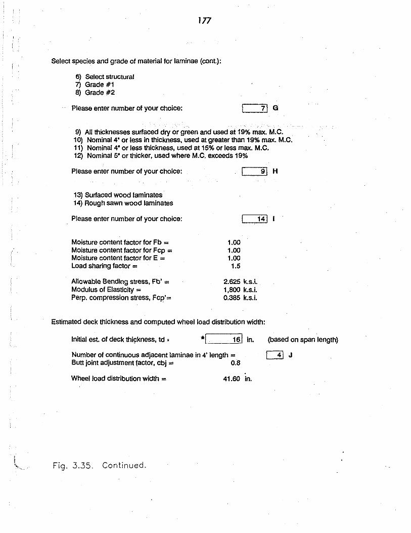
177
Select species and grade of material for laminae (cont.):
6) Select structural 7) Grade #1 8) Grade #2
Please enter number of your choice: ~-7~\ G
9) All thicknesses surfaced dry or green and used at 19% max. M.C. 10) Nominal 4" or less in thickness, used at greater than 19% max. M.C. 11) Nominal 4" or less thickness, used at 15% or less max. M.C. 12) Nominal 5" or thicker, used where M.C. exceeds 19%
Please enter number of your choice: '----'9'-'l H
13) Surfaced wood laminates · 14) Rough sawn wood laminates
. Please enter number of your choice:
Moisture content factor for Fb = Moisture content factor for Fcp = Moisture content factor for E = Load sharing factor =
Allowable Bending stress, Fb' = Modulus of Elasticity = Perp. compression stress, Fcp'=
1.00 1.00 1.00
1.5
2.625 k.s.i. 1,800 k.s.i. 0.385 k.s.i.
Estimated deck thickness and computed wheel load distribution width:
Initial est. of deck thigkness, td ' *~I ___ 16~! in.
Number of continuous adjacent laminae in 4' length = Butt joint adjustment factor, cbj = 0.8
. Wheel load distribution width = 41.60 In.
(based on span length)
[3) J
t ' Fig. 3.35. Continued.

178
Computed design live load and dead load moments:
Dead load of timber deck = Dead load of curb, railing, etc.= Dead load of wearing surface = Total design dead load =
Design dead load moment = Maximum design live load moment = Total design moment (DL + LL) =
43,333 lbs 4,625 lbs
22.500 lbs 70,458 lbs
220.18 ft-kips 103.68 ft-kips 323.~ ft-kips
Computed required deck thickness based on allowable flexural fiber stress:
Effective section modulus, S = 1774.93 in. A 3
Flexural bending stress, Fb = 2. 19 k.s.i.
Allowable Bending stress, Fb' = 2.625 k.s.i.
Check: Fb < Fb' ? Deck is sufficient in flexure.
Computed cheek of live load deflection:
Effect.'ve deck moment of inertia, I = 16329.39 in. "4
Live load deflection, DELTAL = 0.38 in.
Allowable live load deflection = l./500 = 0.6 in.
Check DELTAL < allowable deflection? Deck is sufficient for deflection.
_Computed dead load deflection .and camber:
Dead load applied to deflection: 65,833 lbs
Long term DL deflection, DELTAD = 0.91 in.
Proposed design camber = 2.72 in.
Fig. 3.35. Continued.
I j I

179
Computed required level of prestress force:
Case A - Transverse bending:
Transverse bending moment, Mt = 708.77 in.-lbs/in.
Minimum pr'estress force, p = 16.61 . p.s.i.
Case B - Transverse shear:
Transverse shear force, Vt =; 158.08 lbs/in.
Coefficient of friction, mu = 0.45
Minimum prestress force, p "' 32.93 p.s.i.
Case B controls - minimum interlaminar prestress force "' 32.93 p.s.i.
Check: Minimum prestress force must be >"' to: 40.00 p.s.i.
lntial prestress force applied at construction "' 100.00 p.s.i.
Select size and spacing for prestressing elements:
Input trial value for tendon spacing: 50.001 in. K
Area of steel must be >"' 0.76 in"2
Area of steel must be<= 1.28 in"2
1) 5/8', 150 ksi tendon 2) 1 •, 150 ksi tendon 3) 1 1 /4 •, 150 ksi tendon
Please enter number of your choice: 21 L
Area of steel rod, As = 0.85 in. "2 Rod size is OK
Force in prestressing tendon, Fps= 80,000 lb/in. "2
Fig. 3.35. Continued.
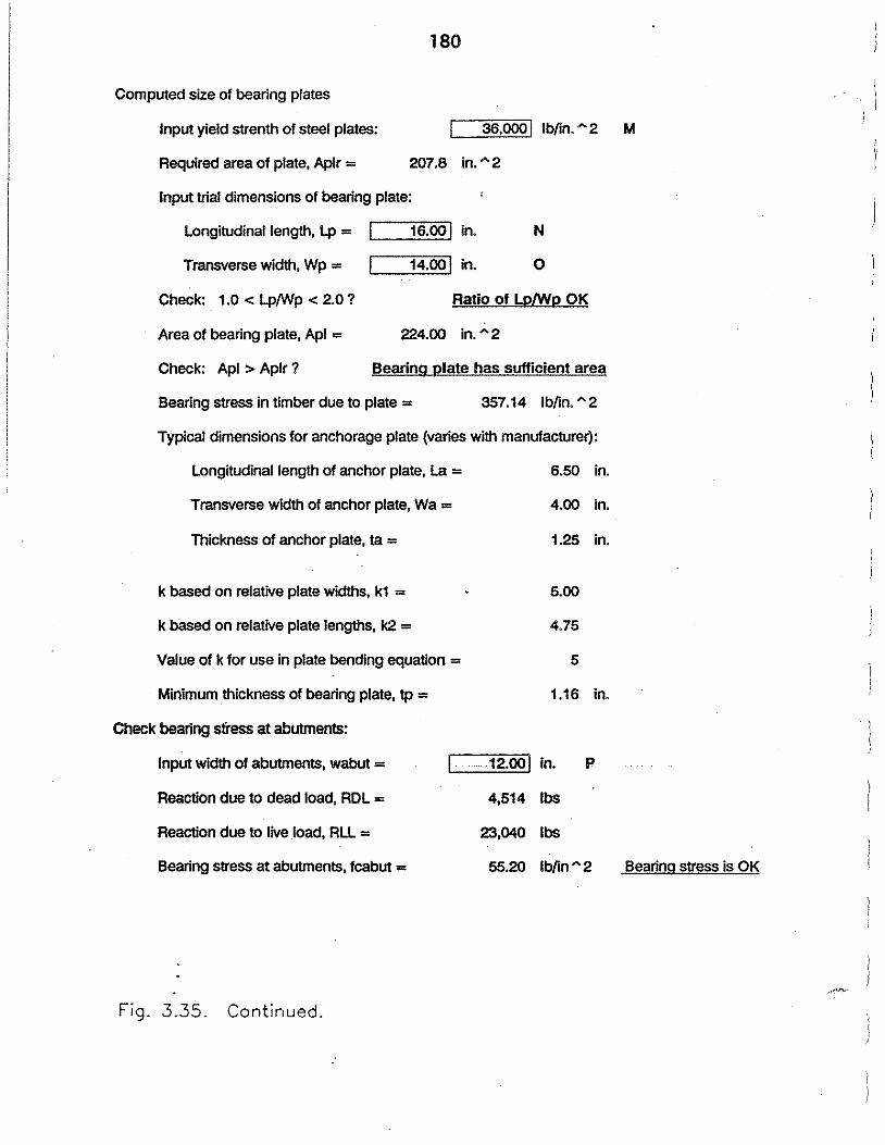
180
Computed size of bearing plates
Input yield stren1h of steel plates: 36,000 I lb/in."' 2 M
Required area of plate, Aplr = 207.8 in. "2
Input trial dimensions of bearing plate:
Longitudinal length, Lp =
Transverse width, Wp = 16.ool in.
14.ool in.
N
0
Check: 1.0 < Lp/'Np < 2.0? Ratio of LP/WP OK
Area of bearing plate, Apl = 224.00 in. "2
Check: Apl > Aplr ? Bearing plate has sufficient area
Bearing stress in timber due to plate = 357.14 lb/in." 2
Typical dimensions for anchorage plate (varies with manufacturer):
Longitudinal length of anchor plate, La = Transverse width of anchor plate, Wa =
Thickness of anchor plate, ta =
k based on relative plate widths, k1 =
k based on relative plate lengths, k2 =
Value of k for use in plate bending equation =
Minimum thickness of bearing plate, tp =
Check bearing stress at abutments:
Input width of abutments, wabut =
Reaction due to dead load, RDL =
Reaction due to live load, RLL =
Bearing stress at abutments, fcabut =
Fig. 3.35. Continued.
6.50 in.
4.00 in.
1.25 in.
5.00
4.75
5
1.16 in.
p 12.ool in.
4,514 lbs
23,040 lbs
55.20 lb/in A 2 Bearing stress is OK

181
Summary of Design Values ··~·,;~
Length, L = 25.00 ft
Width, W= 26.00 ft
Design live loading: MSHTO HS20
Lumber species: Douglas fir-larch
Lumber grade: Grade #1
Maximum moisture content: 19% maximum
Lumber condition: Rough sawn laminates
Thickness of deck, td = 16.00 in.
Stressing system: 1 in. dia., 150 ksi
Spacing= 50.00 in.
Rod anchorage system:
Yield strength of steel = 36.00 k.s.i.
Bearing plate (inches): 16.00 x 14.00 x 1.16
Anchorage plate (inches): 6.50 x 4.00 x 1.25
Stresses and deflections:
Bending stress, fb = 2.19 k.s.i.
Allowable bending stress, Fb' = 2.63 k.s.i.
Live load deflection, deltaL = 0.38 in.
Allowable LL deflection, l/500 = 0.60 in.
Dead load deflection, deltaD = 0.91 in.
Design camber = 2.72 in.
Fig. 3.35. Continued.

182
Summary of Design Values, cont.
Tensioning system:
Minimum prestress force, p =
Force @ construction, pi = Force .in stressing tendon, Fps =
Bearing stress @ anchorage =
Bearing stress at abutment =
Allowable bearing stress, Fcp' =
F. ., ., 5 1g . ..J • ..J • Continued.
40.00 p.s.i.
100.00 p.s.i.
80,000 lbs
357 p.s.i.
55 p.s.i.
385 p.s.i.
I . I

183
The spreadsheet automatically computes this initial deck thickness based on these values. This
initial · thickness estimate may be revised lf the ensuing calculations show a deck which is
significantly over-designed. The spreadsheet deck thickness can be changed by over-writing the cell
which contains the automatically computed value (Input*).
The wheel load distnbution width, D.., is taken as:.
D., = cbtftire contact width + 2tJ where the tire contact width is determined from Art. 3.30 of the AASI:ITO Specifications (2). The
butt joint adjustment factor, c.;. is determined from Art. 3.25.S.4 of the Guide Specifications (1) as:
c - I bJ - (; + 1)
where j is the minimum number of continuous laminae in any four foot longitudinal length (Input
J).
4. Compute the design live and dead load momenlll. The dead load of the deck is based on the
assumed thickness, along with any additional dead load from a wearing surface (lf employed),
guardrail, curbs, and other fixtures. The total dead load moment should be calculated for a width
. of the deck equal to the wheel width plus twice the deck thi.ckness.
The maximum live load moment due to a wheel line should be calculated. A table has.been
developed which gives the maximum live load moment for various span lengths and design loadings.
For AASI:ITO live load moments, see Appendix A of the AASI:ITO Standard Specifications (2);
for Iowa legal truck live load moments, see Appendix B of this manuaL
· 5. Determine the required declc thickness based on allowable fl.emial stress under combined dead and
live loads. The dead load and live load moment diagrams should be combined to determine the
maximum total bending moment, M.,.. In the case of a simple span bridge, the maximum moment
is assumed to be the sum of the maximum dead load moment, Moi.. and maximum live load
moment, Mu. (since MoL and Mu. occur at different locations).
In the case of a simple span bridge, the dead load moment at any position along the span is given
by:
where WoL is the uniform dead load over the wheel load distnl>ution width, x is the position along
the span, and L is the total span length. The maximum live load moment, Mu., occurs when the
center of gravity of the design wheel loads and the nearest heavy wheel load are positioned

184
equidistant Crom the centerline of the span. An expression for the maximum live load moment and
shear for an HS-20 loading has been developed and is presented in Table 3.26. The spreadsheet
automatically calculates the design dead and live load moments based upon the span length, design
vehicle and any wearing surface, etc. whicli has been included.
An idealized portion of the deck, with width equal to D.,, and thickness t,, shall be assumed
to resist the total maximum momeiiL The flexural stress, f,,, is given by:
M"" !b=s
where the effective section modulus, S, is given by:
2
-D"-.,c"""bf_d ' s = 6
If the calculated flexural stress exceeds the allowable value computed in design Step 2), either
the deck thickness, t,, must be increased (see design Step 7)), or a higher grade of lumber (one
which has better material properties) inust be used. If f,, is signifieantly less than the allowable
stress value, a thinner deck or a· lower-grade material may be more economical In any case, changes should not be made until the live load deflection is checked.
6. Cleek the live load deflcctlon. Live load deflection, '1u.. is computed by standard elastic analysis
methods for one wheel line of the design vehicle. The deflection is due to this wheel line applied
over a width equal to D., and modified by a factor of 1.15 (See Appendix A, Ref. 1. The live load
deflection is given by:
A = ~ffection coeff. u. 1.15 E1 I
where E' is the modulus of elasticily of the laminae, corrected for moisture contenL The
deflection coefficient can be found in Table 16-8, Ref. 66, and the effective. deck moment of inertia,
I, is given by:
' I.
I

185
Table 3.26. Maximum moments and shears for HS-20 loading.
Span Length, (ft) Moment, (ft-kips)
0. 23.9 SL
23.9. 33.8 16L + 784/L • 224
33 .. 8. 145.6 18L + 392/L • 280
>145.6 0.08L2 + 4.SL
Span Length, (ft) Shear, (kips)
0 -14 32
14 -28 64. 448/L
28-127.5 72. 672/L
>127.5 0.32L + 26
An abbreviated version of the deflection coefficient table is given in Table 3.27. To obtain
the live load deflection for one wheel line in inches, divide the deflection coefficient by EI (!b
in'). The live load deflection should be compared to the AASHTO allowable value of L/500.
The spreadsheet automatically computes this deflection and compares it to the allowable
value.
7. Revise thlckness it necesaazy. If the flexural stress and/or live load deflection computed in
steps 5) and 6) are significantly different from the allowable values, a new thickness should
be assumed and the calculations for dead load, distribution width, flexural stress, and live load
deflection repeated until acceptable values are attained. Note, any assumed thickness values
should be taken as multiples of the common lumber dimension (714 in., 8 in., 914 in., 10 in.,
etc.).
Spreadsheet users need to enter a larger deck thickness value (Input •) and the
remaining calculations will be performed automatically.
8. calculate dead load dcfledlon and camber. The dead load deflection of the deck is calculated
assuming the dead load weight from a width of the deck equal to the wheel width plus twice the
deck thickness is resisted bya width of the deck equal 10 the distnbutionwidth, D •. The dead load
deflection, b.01., can be cofnputed as:

186
Table 3.27. Deflection coefficients for HS-20 live loading.
Span Length, (ft) Deflection Coefficient
10 S.16 x 108
lS 1.94 x 10'
20 4.61x10"
22 6.40x 10'
24 9.38x10•
26 1.30 x 10¹⁰
28 1.74 x 10¹⁰
30 225 x 1010
32 285 x 1010
34 3.53 x 10¹⁰
36 4.31x10¹⁰
38' S.19x1010
40 6.18 x 101•
42 7.34 x io10
44 8.65 x 201•
46 1.01x10¹¹
48 1.17 x 10¹¹
so 1.34 x 10¹¹
SS 1.84x10¹¹
60 24S x 1011
65. 3.18 x 10¹¹
70 4.03 x 10¹¹
1S S.02x1011
As mentioned earlier, one of the benefits of including butt joints in the design of the
stresslam bridge is that camber can be built-in to offset the effect of dead load deflection. If

187
camber is to be used, Ritter (66) has recommended the design camber should be 34oL· This
calculation also is performed automatically by the spreadsheet.
9. Determine the requlred 1eYe1 of prestresa to be 1l8Cd ln laminating. In the Guide Specifications
(1), the required prestress force to be used in laminating is given in Article 13.11.1. This force
is the uniform force between the laminates, not the force in the individual post-tensioning
tendons.
Two conditions must be satisfied by the post-tensioning system. First, sufficient pres tress
force must be applied to offSet the effect of transverse bending stresses. The amount of force,
p (in psi), required to satisfy this first condition is:
where the transverse bending moment in in.-lbs/in., Mr, is given by:
for one lane bridges:
for two lane bridges with L < 50 ft:
o.1eM,H M- -T- 1000 L
and where M, = the longitudinal moment caused by a single wheel line in in.-lbs. and b = half
of the bridge deck width in inches.
The second condition which must be satisfied is that sufficient prestress force must be
applied to resist any interlaminar slippage due to transverse shear. The required pres tress
force, p, in psi, shall be computed as:
where µ is the coefficient of interlaminar friction and is equal to 0.35 for surfaced wood and
0.45 for rough sawn wood. The transverse shear, VT, in lbs/in., shall be taken as:
p b VT= -(10.4- -)
1000 L
where P is the maximum single wheel load in lbs.

188
The initial prestress applied to the deck must compensate for prestress losses due to creep
and relaxation. The initial minimum compressive force, p., shall be equal to 2.Sp. The deck
shall be prestressed to the same level during the second week and again between the fifth and
eighth week after the initial stressing. The spreadsheet automatically performs these
calculations.
10. Select a spacing ror the prestresslng elements. The spacing of the prestressing elements should
be based on the span length and the maximum allowable spacing of 60 in. (see Article 13.11.2.2,
AASHrO (2)). Table 3.28 can be used to determine an approximate post-tensioning tendon
spacing (Input K).
Table 3.28. Approximate spacing for prestressing rods.
Rod spacing, (in.)
t, (in.) %'in.+ rods l" in.+ rods 1 v.• in.+ rods
Max. Min. Max. Min. Max. Min.
7V. 41 24 - - - -8 37 22 - - - -
9V. 32 19 - - - -10 29 18 89 53 - -
11V. 26 16 79 47 - -12 25 15 74 44 - -
13V. - - 67 40 99 59
14 - - 64 38 94 56 .
15V. - - 59 35 86 51
16 - . 56 33 82 49
11. Size the prestresslng elements. The type of prestressing system to be used miJst be selected by
the engineer. The most common means of prestressing utiliz.es high strength threaded steel
rods.
Each element, spaced as determined in Step 10, must be able to provide the initial
prestressing force for an area determined by the deck thickness times the element spacing. The
compressive force in the rod is then calculated as the area {thickness x spacing) multiplied by
the initial prestressing force. The minimum area of the prestressing element must satisfy the
following equation (Eqn. 13-26 and 13-27, AASHrO (1)):
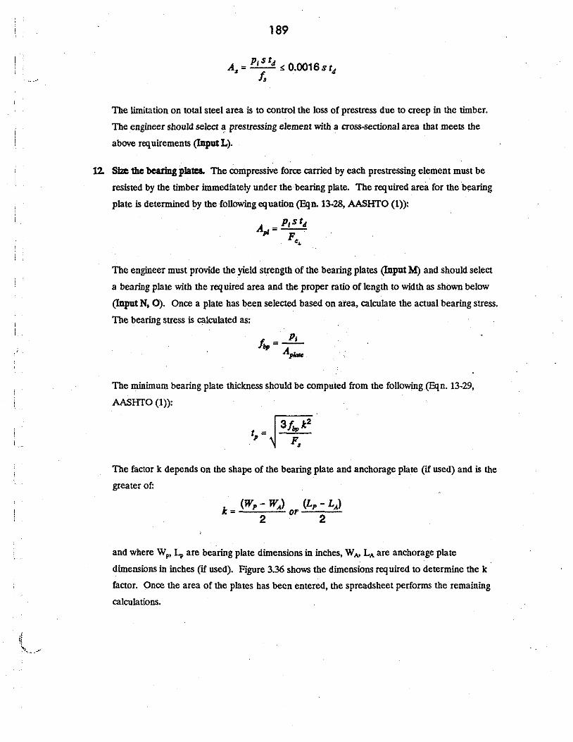
.......
189
p.sr4 A,=-' - ,; 0.0016st4 f.
The limitation on total steel area is to control the loss of prestress due to creep in the timber.
The engineer should select I! prestressing element with a cross-sectional area that meets the
above requirements (Input L).
12 Size the bcarlng pla1CS. The compressive force carried by each prestressing element must be
resisted by the timber immediately under the bearing plate. The required area for the bearing
plate is determined by the following equation (Eqn. 13-28, AASHTO (1)):
A _ p1st4
pl - -----,. F • •
The engineer must provide the yield strength of the bearing plates (Input M) and should select
a bearing plate with the required area and the proper ratio of length to width as shown below
(Input N, 0). Once a plate has been selected based on area, calculate the actual bearing stress.
The bearing stress is calculated as:
The minimum bearing plate thickness should be computed from the following (Eq n. 13-29,
AASHTO (1)):
t = ~ 3/,,,,k2 P F •
The factor k depends on the shape of the bearing plate and anchorage plate (if used) and is the
greater of:
k = (Wp - WA) OT (Lp - LA) 2 . 2
and where W,, I.., are bearing plate dimensions in inches, W,., LA are anchorage plate
dimensions in inches (if used). Figure 3.36 shows the dimensions required to determine the k
factor. Once the area of the plates has been entered, the spreadsheet performs the remaining
calculations.

190
I ,,.- '.1
Bearing Plate - Anchorage plate
Lp
Fig. 3.36. Dimensions required to determine k factor.

191
13. Child: bearing stress at abutment The compressive stress on the abutment should be checked
against the allowable compressive stress perpendicular to the grain, F,,. For this type of bridge,
a timber abutment cap beam over piles (either steel or timber) is normally used. The design of
the piles is left to the designer. Assume a 12 in. wide capbeam unless a more exact value is
known.
The dead load reaction at the abutment, RDL> is computed as one half of the total dead
load on the structure from the deck, the wearing surface (if any), and any curbs, rails or
hardware which is used.
The live load reaction to the abutment, Ru.. can be found in Appendix A, AASHTO (2)
for the appropriate span length.
3. 7.9.6. &le
For illustration, an example stresslam bridge will be designed. The spreadsheet input and output for
this example is shown in Fig. 335. The following criteria will apply to the example bridge:
Length = 25 ft c-c of bearings
Roadway width = 24 ft
Bridge width = 24 ft roadway + 2 ft allowance for curb and/or rail = 26 ft
Existing abutments - bearing length = 24 in.
1. Define geometrlc requirements and design loads. Set L = 25 ft (A). W = 26 ft (B)
Use HS-20 live loading (C):
From Table 16.$, Ref. 47:
Maximum LL moment = 103.68 ft-k
Maximum LL reaction = 23.04 k
LL deflection coefficient= 1.11 x 101•
Use 3 in. asphalt overlay for wearing surface (D and B):
Calculate DL of wearing surface:
DI...,,.,,;,,, = (37 ft)(26 ft)(3/12)(150 lb/ft') = 34,425 lbs ..
2. Select apedca and grade of timber to 1lSC. For this example, choose Grade #1 Douglas fir-larch
(F, G, H and I):
From the 1989 AASHTO specifications (2), Table 13.2.lA:
F. = 1750 psi
F._ = 385 psi
E = 1,800,000 psi

192
Apply modification factors to .material properties:
Fb = F. C..,. Cts
E' = E C..S The moisture content factor, CM can be found in Table 5.7, Ref. (66). Each of the three design
properties can have a different value for ~. so caution is advised.
The load sharing factor, Cts, is determined by the grade of lumber used and can be found in
Sec. 13.2.7, AASHTO (1).
For this example:
Cts = 1.50 c.... = 1.00
CMP.,_ = 1.00
The revised design properties for this example:
Fb = (1750)(1.00)()..50) = 2625 psi
F.,_' = (385)(1.00) = 385 psi
E' = (1,800,000)(1.00) = 1,800,000 psi
3. Estimate deck thickneM and determine wheel load d1'1trlbution width.
Span = 25 ft thus estimated t.t = 14.00 in.
Wheel load distn1mtion width:
D = c.1(wheel width + 2 t.t)
Article 3.30, AASHTO specifications:
Tire contact area = 0.01 P
For HS-20 design load, P = 16,000 lbs.
So tire. contact area = (0.01 )(16,000) = 160 in. 2
kngth in direction of traffic _ _j_ width of tire - 2.5
Length = 0.4 width, so 0.40 vi' = 160 in.2
For this example, w = 20.00 in.
If butt joints are positioned every 4th laminae (l),
. 4 cbi = _J_ = -- = 0.80
j+1 4+1
I ., I I .
I

193
The wheel load distribution width, D.- is:
Dw = (0.80)(20.00 in. + 2(14.00 in.)) = 38.40 in.
4. Compute cleslgn dead and live load momen1B.
Dead load of timber deck = (25 ft)(26 ft)(14/12)(50 lb/ft')
= 37,917 lbs.
Dead load of curb, railing, etc. = (25 ft)(185 lb/ft)
= 4625 lbs.
Dead load of wearing surface = 22,500 lbs.
Total dead load = 65,042 lbs
Distnbuted dead load,
Design DL moment,
65,042 lbs WDL = 25ft = 2602 lbs/ft
MDL= (2.602 k[ft)(25ft)2 = 203.3ft-k 8
Design live load moment, Mu. = 103.68 ft·k
Total design moment = 203.3 + 103.68 = 306.98 ft-k
S. Compute flemra1 stresa and oompaic to allowable.
Effective section modulus, S:
S = D t2 = (38.40 in.)(14 in.}2 = 1254 in.3
6 6
Actual flexural stress in deck, f.:
fb = Mtot = (306.98ft-k)(12in/ft) = 2.94 kjin.2 s . 1254 in.3
Check: 2.94 ksi > 2.625 ksi :. NO GOOD -> recycle.
Note: don't recycle until after checking LL deflection
6. . O!ccli: live load deflectlon.
· I = 1.15 x I used for stress calculation
(see Article 3.25.5.3, AASHTO (2))
1 = 1.15 D t3 _ (1.15)(38.40 in.)(14)3 in. = 10 098 in.4
12 12 •

194
4~ = Deffection coejf. = 1.11x1010 = 0_61 in.
E1I (1,800,000 lb{in.2)(10,098 in.4)
Compare to allowable deflection = USOO = 0.60 in.
Check: 0.61 in. > 0.60 in. :. NO GOOD -> recycle.
7. Rcvlsc thickness If nccessaiy. Try a deck thickness of 16 in. (Input•). For brevity, the
calculations will be omitted for the 2nd cycle of calculations.
For a deck thickness of 16 in.:
D,, = 41.60 in.
Dead load of timber deck = 43,333 lbs.
Total design dead load = 70,458 lbs.
Total design moment (DL + LL) = 323.86 ft-k
Effective section modulus, S = 1774 in3
Flexural bending stress, F, = 2.19 ksi
Check: 2.19 ksi < 2.625 ksi :. OK for flexure
Check live load deflection:
I = 16,329 in•
Live load deflection = 0.38 in.
Check: 0.38 in. < 0.50 in. . :. OK for live load deflection.
8. Calcu1a1C dead load dellcalon and c:ambcr.
I= (41.60 in.)(16in.)3 = 14,199 in." 12 .
w = DLdtd: + DL,.,,,,;,,, = 43,333 + 22,500 = 219•4 lb{in. D£ ungth, in. (25)(12)
!J.D£ = 5woiL
4 = __,(_.5).._(2_19_.4({_.....(25_...,)(_12 .... >r.__ = 0•19 in.
384 E1 I (384)(1,800,000)(14,199)
Camber should be set to 3AoL = 3(0.91) = 2. 72 in.
9. Dctermflle required 11=1 of prestn:sa fon:c.
Case A • transverse bending:·
Mr= 0
•79
M, (-£.)0·5 = (0.79)(103.68)(12)( 13)0·5 = 708.8 in-lb{in. 1000 L 12
i
.···

195
p = 6 MT = (6)(708.8) = 16.61 lbfin.2 ti (16)2
Case B • transverse shear:
For an HS-20 load, P = 1~,000 lbs., so:
v = _L(10 4-k) = 16000 (10 4- <13><12» = 15810 lb/" T 1000 . L 1000 . (25)(12) . Ill.
p= 1.5 VT= (1.5)(158.1) =32.94lb/in.2 µ t4 (0.45)(16)
Note: AASHTO requires that p must be ;,, 40 lb/in.2, so set p = 40 lb/in.2
The initial prestressing force, p; = 2.5 p = 100.0 lb/in.2
10. Select size and spacing of prestresslnJ!: elements.
Two conditions must be satisfied:
A,.: 0.0016 s t 4
Try a spacing of 50 in. (K):
A l! P1 s t4 = (100)(50)(16) . = 0.76 in2 ' 0.70f P'I (0.70)(150,000 psi)
A," 0;0016 s t4 = (0.0016)(50)(16) = 1.28 in.2
Check: s s 60 in. :. OK. (see Art. 13.11.2.2, AASHTO (1))
11. Si1lc the preslml8ing elements. For this example, use 1 in. diameter, 150 ksi rods (L).
The force in the prestressing rods is computed as:
F,., = P; s t4 = (100lb/in.2)(50 in.)(16 in.) = 80,000 lfuo

196
12. Si2JC bearing and anchorage plate. The required area for the bearing plate is calculated as:
, _ P1 s t4 _ (100)(50)(16) _ 207 a . 2 "P1- - F'.. - 385 lb/in.2 - • in.
<L
Assume A36 steel (M)
Try I;. = 16 in., w. = 14 in. (N and 0) Ai>L = (16)(14) = 224 in.2
L 16 Check (advisory): 1.0 ~ .:::L = - = 1.14 ~ 2.0 .·. OK
WP 14
Actual bearing stress is calculated as:
fbp = P1S t4 = (100)(50)(16) = 357.1 psi APL 224
Anchorage plate design:
Exact size depends on manufacturer.
Typical values (from Table 9-6, Ref. 66):
For 1 in. dia. rod: WA = 4 in., LA = 6.S in., tA = 1.25 in.
Calculation of bending stress in bearing plate:
k = w,-wA = 14-4 = 5 2 . 2
or
_ L,-LA _ 16-6.5 = 4•75 - 2 - 2
Use k = S.
The thickness of the bearing plate must be great enough to prevent bending in the plate.
F, = O.SS F1
For A36 steel, F, = 19,800 psi
t = ~ 3/,,,,k2 = , F ,
(3)(357.1)(5)2
= 1.16 in.2 19,800

197
Use t, = 1.25 in.
· 13. Clleck bearing stresa at abutments. Assume a timber cap beam width of 12 in. for this example.
Reaction due to dead load, RoL:
Ru • i ( 41 ·~ m) (25 ft) I <1 ~:-l (50 lb-ft°) + (31~) (150 lb{ft")] • 4,513 lbs. • 451 k
Ru. = 23.04 k. (from Table 16.8, Ref. 66).
f, = RoL+Ru = 4.51 + 23.04 = 55.2 . CJ. D., lb (41.60)(12} psi
Check: 55.2 lb/in.2 < F'.,. = 385 lb/in.' :. OK.
SummalyofDeslgn Values:
Length = 25 ft, Width = 26 ft
Design loading: AASHTO HS-20, 2 lanes wide.
Lumber: Grade No. 1, Douglas fir-larch
Deck thickness = 16 in.
Stressing system:. l in. dia. 150 grade rods at 50 in. centers
End rods 25 in. from end of bridge
Rod Anchorage system: Use 16 in. x 14 in. x 1.25 in. bearing plate
Use 4 in. x 6.5 in. x 1.25 in. anchor plate
Both plates of A36 steel
Stresses and deflections:
f. = 2.19 ksi
F.' = 2.625 ksi
Au. = 0.38 in.
AoL = 0.91 in.
Camber = 2. 72 in.
P=40psi

P1 = 100 psi
F .. = 80,000 lbs
t., at anchorage = 357 psi
C., at bearing = 55 psi
F.,.' = 385 psi
3. 7.10. Gluc.I amlnaled Timber Beam Bridge
3.7.10.1. Background
198
In the past few years, a number of new wood products, such as structural composite lumber, have
been developed. Although there are several different techniJ. ues for manufacturing large members from
small timber laminates, this report will concentrate only on glue-laminated (glulam) timber beam and
timber deck construction. The are two reasons for this limitation. First, glulam beams have been in use
since the mid-1940's and the design methodology for this type of member is recognized by AASHTO.
Secondly, systems such as laminated veneer lumber (L VL), while showing much potential for future use,
have not been used in actual bridge construction. No formal specifications have been developed for L VL
beam bridges at this time. Additional information on the use of L VL for bridges can be found in (Refs. 5,
77, 78, 98).
Glue-laminated panel bridge decks, which were developed at the USDA Forest Products Laboratory
in the 1970's, are the most common type of timber deck in use today. The panels are normally S to 8 in.
thick and 3 to S ft wide. Glulam decks are much stiffer and stronger than conventional nail~laminated
decks because of the rigid bond between laminations.
Glue-laminated (glulam) timber beam bridges (see Fig. 3.37) are constructed essentially the same as
an ordinary sawn lumber beam bridge with the exception of the beams themselves. Glulam beams are
manufactured from 1-1/2 or 1-3/8 in. thick timber lamintes which are bonded together on their wide faces
with waterproof structural adhesives. They are available in a number of standard widths from 3 to 14 1/4
in., while the depth of a glulam beam is limited only by the size of the pressure treating facility and
transportation problems. Although glulam timber beams can be fabricated in essentially any shape, the
most economical shape is a standard size beam which is available from a number of fabricators (66).
Glulam timber beams offer several advantages over ordinaiy sawn lumber beams. Because the depth
of glulam beams are greater, a given bridge will require fewer beams. Also the glulam beams are able to
span greater distances than sawn lumber beams. Glulam beams are able to span more than 140 ft, but are
more commonly used for span lengths of 20 to 100 ft.
Glulam timber bridge beams are fabricated with horiz.ontally laminated bending combinations given
in Table 1 of AITC 117 - Design (4). These combinations provide the most efficient beam section where
primary loading is applied perpendicular to the wide face of the laminations (66).
,,....., i \.. ) I

199
.1 '
< (i! Bridge
Glulam deck I Wearing surface
l< Equally spaced glulam beams >I
Fig. 3.37. Typical section of glulam timber beam bridge.

200
3.7.10.2. Design criteria. ,,.----.,,
The design material presented in this section is based on the AASHTO Standard Specifications for i Highway Bridges (2). Much of the material presented in this section is based on work presented by Ritter
(66).
The glulam timber beam and glulam timber deck design procedures descn'bed in this manual are
applicable only to AASHTO Group I loads. In this case, it is assumed that the design will be controlled by
a combination of dead load and standard AASHTO truck loads. Dead load is assumed to include the
weight of the timber itself, plus a 3 in. asphalt wearing surface a~d any guardrails or other attachments.
Material properties for various sawn lumber species are taken from the 1986 edition of the National
Forest Products Association's Design Values for Wood Construction (51). Although this particular
discussion applies only to Southern Pine and Douglas Fir, the basic design principles could be applied to a
number of species. Combination symbols for glulam timber are taken from AITC 117 ·Design (4).
Timber components used in this procedure are assumed to be pressure treated with an oil-borne
preservative.
The AASHTO specifications do not specify live load deflection limitations for either glulam beam or
deck design. Deflection guidelines :which follow are based on common design practice and experience.
Perhaps the most influential factor in the economic design of a glulam timber beam bridge is the
beam configuration. The number and spacing of beams affects the size and strength requirements for the
beam and deck elements which in tum significantly influence the cost of materials, fabrication and
construction. Three primacy factors influence the beam configuration in glulam bridges: site restrictions,
. deck thickness, and live load distn'bution to the beams. Each of these factors will be discussed briefly in
the following paragraphs.
Site restrictions. The most efficient beam is a deep, relatively narrow section. In some cases,
however, this cross-section may be impractical due to overhead clearance limitations. In such cases,
shallower beams are employed which in tum requires the number of beams to be increased for the desired
load capacity. These shallow beams are generally arranged in several closely spaced groups. In most cases,
though, a deck-type structure (See Secs. 3.79 and 3.7.11) would be more economical for sites with clearance
problems.
Deck thickness. As beam spacing increases, deck flexural stresses and deflections increase, requiring
either a thicker deck, or one with a greater flexural stiffness. Glulam decks are available in standard
member dimensions that increase in 1 ~ or 2 in. increments.
Live load distnoution. The magnitude of the vehicle live load supported by each beam is directly
proportional to the distnoution factor (DF) for that beam. The OF provides an indication of the relative
beam size and grade requirements for different configurations.
The ability of a bridge to distn'bute loads laterally depends on the transverse stiffness of the structure
and the number, size and spacing of beams. Although load distn'bution is influenced by the type and.
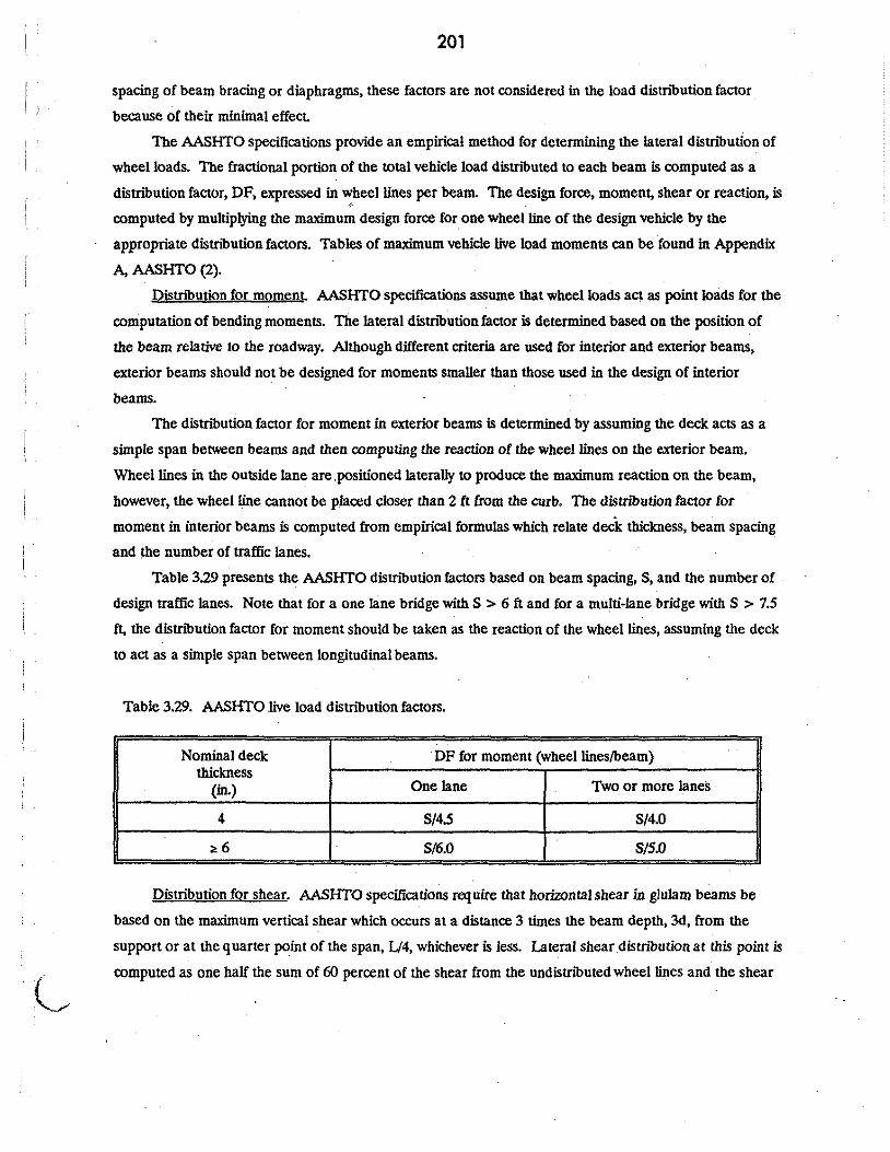
201
spacing of beam bracing or diaphragms, these factors are not considered in the load distnbution factor
because of their minimal effect
The AASHTO specifications provide an empirical method for determining the lateral distnbution of
wheel loads. The fractional portion of the total vehicle load distnbuted to each beam is computed as a
distnbution factor, DF, expressed in "'.,heel lines per beam. The design force, moment, shear or reaction, is
computed by multiplying the maximum design force for one wheel line of the design vehicle by the
appropriate distnbution factors. Tables of maximum vehicle live load moments can be found in Appendix
A, AASHTO (2).
Distnbution for moment. AASHTO specifications assume that wheel loads act as point loads for the
computation of bending moments. The lateral .distnbution factor is determined based on the position of
the beam relative to the roadway. Although different criteria are used for interior and exterior beams,
exterior beams should not be designed for moments smaller than those used in the design of interior
beams.
The distnbution factor for moment in exterior beams is determined by assuming the deck acts as a
simple span between beams and then computing the reaction of the wheel lines on the exterior beam.
Wheel lines in the outside lane are .positioned laterally to produce the maximum reaction on the beam,
however, the wheel line cannot be placed closer than 2 ft from the curb. The distnbution factor for
moment in interior beams is computed from empirical formulas which relate deck thickness, beam spacing
and the number of traffic lanes.
Table 3.29 presents the AASHTO distnbution factors based on beam spacing, S, and the number of
design traffic lanes. Note that for a one lane bridge with S > 6 ft and for a multi-lane bridge with S > 7.5
ft, the distnbution factor for moment should be taken as the reaction of the wheel lines, assuming the deck
to act as a simple span between longitudinal beams.
Table 3.29. AASHTO .live load distnbution factors.
Nominal deck DF for moment (wheel lines/beam) thickness
(in.) One lane Two or more lanes
4 S/4.5 S/4.0 .
;,: 6 S/6.0 S/5.0
Distnbution for shear. AASHTO specifications require that horizontal shear in glulam beams be
based on the maximum vertical shear which occurs at a distance 3 times the beam depth, 3d, from the
support or at the quarter point of the span, U4, whichever is less. Lateral shear distnbution at this point is
computed as one half the sum of 60 percent of the shear from the undistnbuted wheel lines and the shear

202
from the wheel lines distributed laterally for moment. For undistnl>.uted wheel lines, one wheel line is
assumed to be carried by one beam. The live load shear can be expressed as:
where:
Vu.
Vw
Vw
Vu = 0.5((0.6 Vw) + V wJ
= = =
distn"buted live load vertical shear·used to compute horizontal shear (lb).
maximum vertical shear from an undistn"buted wheel line (lb).
maximum vertical shear from the vehicle wheel lines distn"buted laterally as specified for
moment (lb).
Distn"bution for reactions. The live load distn"bution for reactions is computed assuming there is no
transverse distn"bution of wheel loads to adjacent beams. The distn"bution factor, DF, for both interior and
exterior beams is computed as the reaction of the wheel lines at the beam, again assuming the deck acts as
a simple span between longitudinal beams.
Exclusive of site restrictions, beam configurations should be based on economic and performance
considerations for both the beam and deck components. These considerations will vary depending on
material prices, availability, and transportation and construction costs. Table 3.30 provides a general
guideline for the number and spacing of glulam beams.
Several modification factors have been developed to account for the behavior of different timber
species for environmental and loading conditions. Note that the equations developed in this section do not
include the duration of load factor, C,,, or the modification factors for temperature effect, C.. and fire.
retardant treatment, c,,. To reduced fabrication costs, glulam beams should be developed using standard dimensions. Table
3.31 is provided for determining standard size glulam beams.
Table 3.30. Guidelines for number and spacing of glulam beams.
Roadway Number of Beam Deck Moment I Width (ft) beams spacing (ft) overhang (ft) DF
24 5 5.0 . 2.0 1.00
26 5 5.5 2.0 1.10
28 5 6.0 2.0 1.20
34 6 6.0 2.0 1.20 .

203
Table 3.31. Standard glulam beam dimensions.
Net finished width (in.) Nominal width
(in.) Western Species Southern Pine
4 3-1/8 3
6 5-1/8 5
8 6-3/4 6-3/4
10 8-3/4 8-1(2
12 10-3/4 10-1!2
14 12-1/4 . 16 14-1/4 .
3.7.10.3. Design Procedure
The design procedure descnbed in this section is for a glue laminated timber beam bridge. There
are several types of bridge decks which are available commercially, thus .no provision for deck design is
provided. Spreadsheet input parameters refer to the spreadsheet in Fig. 3.38.
1. Define basic a>nflguratlon and design criteria. Several dimensions must be determined:
• Span length, L, from c-to-<: of bearing (Inpnt A).
• Roadway width, W, from inside of curbs (Input B).
Note: in this spreadsheet, the additional width of curbs and/or railing, etc., has been
ignored.
• Number of traffic lanes.
• Number and spacing of beams (computed automatically by the spreadsheet based on
roadway width).
• Deck and railing/curb configuration.
• Design live load vehicle (Input C).
2. Select beam c:omblnatlon symbol and spedea. A preliminary beam combination symbol should
be selected from the AITC 117 - Design manual ( 4) (Input D). Commonly used combination
symbols for glulam beam bridges are presented in Table 3.32.
Based on the combination symbol, the tabulated design properties of the member can be
determined from AITC 117. The allowable bending stress, F,., allowable compressive stress
perpendicular to grain, F"', allowable horizontal shear stress, F ... and Young's modulus, E,,
should be recorded for later use. These tabulated design properties must be reduced for wet-

204
Design of Glue-Laminated Timber Beam Bridges
Input deck geometric requirements:
Input bridge length, L = Input roadway width, W =
Select design live loading:
1) HS20-44 2) HS 15-44
Please enter number of your choice:
Select beam combination symbol and species:
1) 24F-V3 Western species 2) 24F-V4 Western species 3) 24F-V2 Southern pine 4) 24F-V3 Southern pine
· 5) 24F-V6 Southern pine
Please enter number of your Choice:
A B
c
D
Computed design properties (adjusted for wet-use conditions):.
Allowable bending stress, Fbx = Compression perp. to grain, Fcp = Allowable shear stress, Fvx = Young's modulus, Ex =
Select type and thickness of wearing surface:
1) No wearing surface 2) Ashphalt wearing surface
Please enter number of your choice:
Thickness of ate wearing surface (If any):
21
1920 psi 345 psi 144 psi
1.499E +06 psi
3.00/ in.
E
F
Computed dead load moment (Assume 51/8' timber deck):
Dead load of deck panels = Dead load of wearing surface = Total uniform dead load =
21.35 lb/ft,.. 2 37 ,50 lb/ft A 2 58,85 lb/ft A 2
Fig. 3.38. Glulam timber beam spreadsheet, input parameters, and example problem.

205
Beam spacing (based on roadway width) =
Deck overhang (outside beam to face of rail) =
DL moment for interior beams:
Uniform dead load, WOLi = Estimated wt. of beam =
Dead load moment, MDLI =
DL moment for exterior beams:
Uniform dead load, WDLE = Estimated wt. of beam =
Dead load moment, MOLE =
Computed live load moment:
Distribution factor, DFM = Moment due to one wheel line =
Live load moment, MLL =
Computed beam size based on bending stress:
Preliminary allowable stress, Fb' = (Doesn't include CF)
Design moment for interior beams, MTI == Design moment for exterior beams, MTE =
DESIGN ALL BEAMS FOR DESIGN MOMENT =
Required section modulus, tx CF =
Western species - lightest alternative:
294.27 lb/ft 319.60 lb/ft
678.02 ft-kip
339.27 lb/ft 319.60 lb/ft
727.72 ft-kip
1.00 708.09 ft-kip
708.09 ft-kip
5.00 ft
2.00 ft
1920 psi
1,386.1 ft-kip 1,435.8 ft-kip
1,435.8 ft-kip
8,974 in"3
Press <ALT> W to select the lightest beam section.
Fig. 3.38. Continued.

206 Computed lightest section which meets requirements:
Beam width, b = Beam depth, d =
Section modulus, Sx =
Adjusted section modulus, SxCF = Cross section area, A =
12.25 in.
73.5 in.
11,030 inA3
9,018 in"3
900.38 in " 2
Moment of inertia, Ix = 405,338 in "4
Self-weight of beam =
Actual weight of beam < estimated - OK!
Actual bending moment, Mactual =
Bending stress on beam, lb =
1,428.1 ft-kip
1,553.8 psi
Allowable bending stress, Fb' = 1,569.8 psi
BEAM IS SATISFACTORY FOR FLEXURE.
Computed check of beam for lateral stability:
Distance between lateral support, lu = Length-to-depth ratio, lu/d =
Effective length, le =
23.50 ft.
3.84
680.16 in.
18.25
312.63 lb/ft
Beam slenderness factor, Cs = Intermediate beam factor, Ck =
·Lateral stability factor, CL =
26. 72 Intermediate beam
0.927
CL > CF so strength controls design - OK.
Computed check of live load deflection:
Live load deflection, DELTALL =
Allowable LL deflection, L/360 = 1.68 in.
3.13 in.
BRIDGE IS SUFFICIENT FOR LL DEFLECTION.
Fig. 3.38. Continued.
' i

Computed check of horizontal shear:
Uniform dead load on beam =
Dead load vertical shear, VOL =
LL vertical shear computed at distance =
Max. shear due to one wheel .Une, VLU =
Vert. shear distributed laterally, VLO =
Live load vertical shear, VLL =
Total vertical shear, V = VOL + VLL =
Horizontal shear stress, fv =
Allowable shear stress, Fvx =
207
BEAM IS SUFFICIENT FOR SHEAR.
651.90 lb/ft
26,646 lb.
18.38 ft.
25,388 lb.
25,388 lb.
20,311 lb.
46,957 lb.
78.23 lb/in "2
144 lb/in" 2
Computed bearing length and bearing stress (wet-use conditions):
Allowable compressive stress, Fcp =
Reaetion due to uniform load, AOL=
Distribution factor for reaetion =
Reaction due to one wheel line, Rwheel =
Total reaction force, Rtotal =
344.5 lb/in" 2
30,639 lb.
1.00
32,430 lb.
63,069 lb.
Required bearing length = 14.9 in. Use 18.00 in.
Recompute DL reaction, RDLtotal = 31,128 lb.
Total compressive stress, fcp = 286.03 lb/in" 2
BEAM IS SUFFICIENT FOR BEARING.
Computed design camber:
Uniform dead load, wunif = 651.90 lb/ft
Dead load defleetion, OELTADL = 1.88 in.
Minimum design camber = 3.80 in.
Fig. 3.38. Continued.

208
Summary of Design Values -,'l
Geometry and design loading:
Bridge Length, L = 94.00 ft I!
Roadway width, W = 24.00 'ft
Design live load: AASHTO HS20-44
Beam combination symbol: 24F-V4 Western species
Type of wearing surface: Asphalt 3.00 in.
Beam dimensions and properties:
Beam width, b = 12.25 in.
Beam depth, d = 73.5 in.
Beam spacing, S = 5.00 ft
Beam section modulus, Sx = 11,030 in"3
Beam cross sectional area, A = 900.375 in "2
Beam moment of inertia, Ix = 405,338 ln"4
Self weight of beain, wbeam = 312.630 lb/ft
Stresses and deflections:
Actual bending stress, lb = 1,554 lb/in "2
Allowable bending stress, Fb' = 1,570 lb/in" 2
Actual shear stress, fv = 78 lb/in"2
Allowable shear stress, Fvx = 144 lb/in"2
Actual bearing stress, fcp = 286 lb/in "'2
Allowable bearing stress, Fcp' = 345 lb/in" 2
Live load deflection, DELTALL = 1.68 in.
Allowable LL deflection, L/360 = 3.13 in.
Dead load deflection, DELTADL = 1.88 in.
Design camber = 3.80 in.
. . .-~· ,,,
Fig. 3.38. Continued.

209
use conditions unless a watertight deck is used. The computer spreadsheet in this manual is
based on wet-use conditions. The spreadsheet automatically calculates the allowable stresses ·
based upon the combination symbol and species selected.
Table 332. Co/Dmonly used glulam beam combination symbols.
Bridge type Western Species Southern Pine
24F-V3 24F-V2
Simple span 24F-V4 24F-V3
24F-V6
Continuous spans 24F-V8 24F-V5
3. Dclermlne deck dead load and dead load moments. The deck dead load supported by each
member should be computed, This dead load should include such things as the weight of the
deck, railing, wearing surface and hardware. If there is no better estimate available, a
preliminary deck thickness of 6-3/4 in. may be assumed. The difference between the estimated
and the actual member weights is normally insignificant, but should be verified. The existence
and type of wearing surface should be input as B and F for spreadsheet users. The spreadsheet
automatically computes the dead load moment based on these input parameters.
The dead load mc;>ment at any position along the span, M0 .., for a uniformly distnbuted
load can be computed as:
4. Dctermlne liYC load moment. Live load moments are computed for both interior and exterior
beams by multiplying the maximum moment for one wheel line of the design vehicle (whether
based on the desjgn vehicle or the equivalent lane loading) by the appropriate distnbution
factors. Tabulated values of maximum live load moments can be found in Appendix A,
AASHT0(2).
The spreadsheet performs this calculation automatically based upon the span length and
the live load design vehicle chosen.
5. Dctermlne beam size based on bending. The allowable bending stress in glulam timber beams
is controlled by either the size factor, c,, which limits bending stress in the tension zone, or the
lateral stability of beams factor, C.., which limits bending stress in the compression zone. Under

210
normal circumstances, the allowable bending stress in bridge beams is controlled by Cp,
however, both values should be checked.
The adjusted allowable bending stress in a glulam bridge beam can be computed from:
where:
M s c,=-" ~
S. Cp = required beam section modulus adjusted by size factor, Cp (in3).
M = applied dead and live load bending moment (in-lb).
F•' = F,, ~ (psi).
CM = moisture content factor for bending = 0.80.
After an initial beam size has been determined, the dead load moment due to beam self
weight can be computed and the design moment revised. This iterative process should be
continued until a satisfactory beam size has been determined.
The computer spreadsheet performs this iteration automatically, using three cycles to
determine the beam which provides the required flexural capacity. To initiate.the iteration
process using the spreadsheet, press <ALT> W when using western species, and <ALT> S
when using Southern Pine. Spreadsheet users perform (Input G).
The actual applied bending stress can be computed based on the total moment and
compared to the allowable bending stress as:
In addition to satisfying allowable bending stresses, the proposed beam must be checked
for lateral stability. The allowable bending stress, based on lateral stability, depends on the
slenderness of the proposed beam. The slenderne5s factor, Cs, can be computed as:
where:
I., = effective beam length for a single span beam With a uniformly distnlmted load, in. = 1.63
I.+ 3 d
I. = unsupported beam length, in.
d = beam depth, in.
I I

211
b = beam width, in.
Glue laminated timber beams are classified as short, intermediate or long allowable
bending stresses are based on this classification.
Beams with a Cs of 10 or less are classified as short. The capacity of these short
members is controlled by the strength of the wood, rather than stability, and can be computed
from the equation above.
Intermediate beams are those with a Cs of between 10 and C., where C. is given by:
and:
E' = E CM, psi
F.'' = F• CM, psi
c. = 0.956 Hi I
It should be noted that the above equation for C. is based on a modified NOS equation which
takes into account the reCiuced variability of glulam timber beams (52).
Intermediate beams can fail by either an overstress in bending, or by torsional·buckling
from lateral instability. The controlling mode is indicated by the lateral instability of beams
factor, CL> which is given by:
If Q is less than c,, the bending stress is controlled by stability, and Q is the controlling
modification factor. The allowable bending stress is then computed using the following relation:
Long beams are those with a slenderness ratio in the range C. s Cs s 50. Lateral
. stability, rather than strength, controls the design of long beams. As with the intermediate
beams, the allowable bending stress for long beams is a modified NDS equation which takes
into account the reduced variability of glulam timber beams and is computed by:
F.. _ 0.609 E1
b- c2 s

212
6. Cbect liYe load deflection. The live load deflection of a glulam beam bridge can be computed .,.---..,,
by several methods of analysis. For a uniformly loaded simple span, the maximum deflection j occurs at midspan and is computed as:
Sw L4 A - IL
IL - 384E1 I
A reasonable limit on live load deflection is LJ36(). A lower value of deflection should be
considered if the bridge supports a pedestrian walkway or will be covered with an asphalt riding
surface. The spreadsheet automatically computes the live load deflection and compares it to
the allowable value.
7. Cbect horizontal shea•. Dead load horizontal shear is based on the maximum vertical shear
which occurs a distance equal to the beam depth, d, from the support For a uniform dead
load, the dead load shear, V oi.. can be computed as:
where:
VoL =vertical dead load shear at a distanced from the support, lb.
WoL = uniform dead load supported by the beam, lb/in.
Llve load vertical shear is computed at a distance from the support of 3d or LJ4,
whichever is less. The horizontal shear stress due to applied loads, f.. which is 1.SV/A for a
rectangular cross section, must not exceed the allowable stress, which is given by:
where:
V = VoL + Vu.. lb.
A = cross-sectional area of beam, in.2
~ = moisture content factor for shear = 0.875.
It should be noted that the allowable shear stress may be increased by a factor of 1.33 for
overloads in AASHTO Load Group lB. The spreadsheet performs this calculation for the user.
I

213
8. Olcclt lateral and loDgitndinal loada. Ute magnitude and appropriate lateral and longitudinal
loads, such as wind load and centrifugal force will vary among structures. It is the designer's
responsibility to compute and apply the necessary loads in accordance with AASHTO load
groups. The spreadsheet does not consider this step in the design process.
9. Dctermlnc bearlng length &nd strcaa. The bearing area at beam reactions must be large enough
to limit bearing stresses to an acceptable value. The dead load reaction, Rou due to the beam,
deck, wearing surface, railing and hardware should be computed from statics. The live load
reaction at each beam, Ru.. can be computed by multiplying the maximum reaction at one
wheel line by the appropriate distnoution factor for reactions as computed previously.
The required bearing length, L..,,, should be no less than the following:
where:
RoL = dead load reaction, lb.
Ru. = distnouted live load reaction, lb.
b = beam width, in.
F.._ = allowable compressive stress perpendicular to grain, psi
=F.._.CM
The actual applied bearing stress can be computed from:
where A is the bearing area in square inches.
The spreadsheet automatically computes the required bearing length and also computes a
"rounded value• to the next largest 6 in. increment for design purposes.
10. Determine camber. camber is provided to offset the effect of long-term dead load deflection.
The amount of camber to build into a glulam beam bridge is a decision of the designer. There
are two 'rules of thumb" which can be used. For spans less than 50 ft, camber should generally
be 1.5 to 2.0 times the dead load deflection plus 0.5 times the vehicle live load deflection. For
spans greater than SO ft, camber can be estimated as 1.5 to 2.0 times the dead load deflection.
The spreadsheet performs this calculation automatically.

214
3. 7.10.4. Example
The spreadsheet input and ouput for this example is shown in Fig. 3.38.
following bridge will be used:
Length, L = 94 ft from c-to-c of bearings
Roadway width, W = 24 ft from inside of curbs
AASIITO HS20-44 live load (Group I loads only)
3 in. asphalt wearing surface
Visually graded western species
1. Define basic configuration and dealgn c:rilerla.
L=94ft
W=24ft
HS2o-44 design live loading
3 in. asphalt wearing surface
(Input A, B, C, B and F respectiwly.)
2. Sclcc:t beam Combination symbol and apedca.
Select 24F-V4, Western species combination symbol (Input D).
The design properties are:
F.,. = 2400 psi C.. = 0.80
F.,, = 650 psi C.. = 0.53
F,. = 165 psi C.. = 0.87
E. = 1.800 x 10⁶ psi c.. = 0.83
The allowable stresses are computed as:
F .. = F.,.C..Cp
F.,,' = FcpC.. = 345 psi
Fv' = F,.C.. = 144 psi
E' = E.C.. = 1.499 x 10⁶ psi
3. Determine deck dead load and dead load moments.
In this example, the
Dead load of the deck panels and wearing surface can be computed as:
DL = (5.125 in.)(50lbfft3) + (3 in.)(150 lb/ft") = 58.85 lb/ft2 . 12 in./ft

215
The dead load supported by each beam is proportional to the tributary area. For this
example, interior beams support 5 ft of deck width and exterior beams support 5 ft of deck plus
45 lb/ft of curb/rail load.
As a 'rule of thumb" for a glulam beam bridge, the estimated weight of the beam· itself
can be computed as 3.4 times the length of the bridge:
w ... m = 3.4(94 ft) = 319.6 lb/ft
For interior beams:
WDL = (5.0.ft)(58.85 lb/ft) + 319.6 lb/ft = 294.27 + 319.6 = 613.85 lb/ft
MDx., = (613.85 lb/ft)(94 .ft)2 = 678.02ft-k (8)(1000)
For exterior beams:
WDL = 294.27 lb/ft+ 45 lb/ft+ 319.6 lb/ft = 339.27 + 319.6 = 658.87 lb/ft
M = (658.87 lb/ft)(S4 ft)2 = 727.72.ft-k
DL, (8)(1000) .
4. Detcnnlne live load moment The distn"bution factor for moment, DFM, is computed as:
DFM = S = S.O = 1.00 5 5
The live load moment due to one wheel line can be found in Appendix A, AASHTO (2).
For a 94 ft span:
M.bo<I Uno = 708.09 ft·k
The live load moment distnl>uted to one beam is found as:
Mu. = (708.09 ft-k)(l.00) = 708.09 ft·k
S. Detennlne beam size based on tiexure. The AASHTO specifications require that the exterior
beam. be at least as large as the interior beams. For simplicity, one beam size will be designed
for the maximum design moment in the bridge. Conservatively, the maximum dead load
moment will be added to the maximum live load moment, even though these moments do not
occur at the same location in the span.
For this example:
MT = 727.72 + 708.09 = 1435.81 ft-k
The size factor, CF, can not be determined until a. beam size has been determined. In the
iterative process, the s.c, terms will be used; after a preliminary beam size has been
determined, CF will be calculated.

216
Based on an allowable bending stress, F• = 1920 lb/in2, the required section modulus
can be computed as:
For each standard beam width, a beam depth can be determined which will provide the
required S.. The section modulus for this width and depth is computed, and reduced by the
factor c,,. A new beam size is then determined by this iterative process until the required SxC,,
is obtained.
CYCLEl:
Using a 12V. in. wide section, a depth of 66.30 in. is required to provide the required
SxC,,. A standard deplh of 67~ in. is used.
For !his section:
S CF= C, b h2 = (0.825)(12.25 in.)(67.5 in.)2 = 7678.0 in3
• 6 6
This S,C,, is less lhan 8973 in3, lhus we must recycle.
C"'{CLE 2:
Based on !he Cp from !he first cycle, an approximation for Sx can be found as:
_s_. = 8973.83 in3 = 10 872.4 . 3 0.825 ' m
For this section, a deplh of 72.97 in. would be required. Again, a standard deplh of 73~ in. is
used.
For this section:
A third cycle produces !he same section. For a 12V. in. widlh, !he required depth is 73.5
in.
I '1
I r I

217
The computer spreadsheet performs this iterative process for each standard beam width
and determines the lightest possible section which satisfies the required S.CF criteria.
Spreadsheet users should press <ALT> W to perform this iterative procedure and
determine tho lightest secllon whlcb. meell tho aiterla.
For this example, the lightest section is:
Width, b = 1214 in.
Depth, d = 731h in.
Section modulus, S. = (12·25 in.)(73•5 in.)2 = 11,029.6 ;n3 6
Adjusted section modulus, S.4 = 9017.9 in.3
M t f . rtia 1 _ (12.25 in.)(73.5 in.)3 _ 405 338 . 4 omen o me , x -12
- • m
Cross section area, A= (1225 in.)(73.5 in.) = 900.38 in.2
Beam weight, w,,..., = (900.3S in2)(50 lb/ft) = 312.63 lb/ft 144
In this example, the estimated beam weight is gre;lter than the actual weight, thus the
beam cross section obtained is conservative.
The actual bending moment on the beam can be fouild as:
M = (339.27 + 312.63)(94 ft)2 + 708.09 ft-k = 1428.11 ft-k - (8)(1000)
The actual bending stress on the beam is:
~ _ Moctwll _ (1428.11ft-k)(12,000)_15537 . Jb - - - • psi
s% 11,029.6 in3
The allowable bending stress is:
~ = Fk CM C, = (2400 psi)(0.800)(0.818) = 1569.8 psi
Since f• < F.', the beam is satisfactory for flexure. However, the beam must also be
checked for lateral stability.
Check of lateral stability:
The distance between points of lateral support, !,,, is assumed to be 1)4 = 23.5 ft.
The length-to-depth ratio for this configuration is:

218
z. = (23.50 ft)(12) = 3.84 d 73.5 in.
The effective length, J., is:
l, = 1.631. + 3d = 1.63(23.5 ft)(12) + 3(73.5 in.) = 680.16 in.
The beam slenderness factor, Cs, is found as:
c = ~. l,d < 50 = • b2 (680.16)(73.5) = 18.25
(12.25)~
The intermediate beam factor, C., is the largest value of Cs for which the intermediate beam
equation applies. C. is calculated as:
1.499x108 = 26.7:! 1920
Since Cs < C., the beam is classified as an intermediate beam.
The lateral stability factor, Ci.. for an intermediate beam is given by:
For this example, Ci. < Cp, so strength, rather than lateral stability controls the design.
Therefore, no changes are required in the previous calculations.
6. Checll: li\'e load deftcc:tlon. The live load deflection due to an HS2().44 truck can be computed
as:
A = Deflectioncoejf. = . 1.02x1012 = 1.6Sin. . u E1 I. (1.499 x 10⁸ ps1)(405,338 in4)
The allowable live load deflection is:
A·u = ....f._ = (94 ft)(12) = 3.13 in. - 360 360
Since Au. < the allowable value, the bridge is adequate with respect to live load deflection.
I

=~.
219
7. Chedt horizontal shear. The dead load vertical shear is based on the loading shown in Fig.
3.39.
The dead load vertical shear, You is computed as:
VDL = WDL(L-d) = 651.9 lb/ft ( 94 ft - 73·5 in.)= 26,646 lbs. 2 2 12
Live load vertical shear is computed from the maximum vertical shear occurring at the
lesser of 3d or 1./4 from the support.
For this example,
3d = 3(73.5 in.) = 220.5 in. = 18.38 ft -> controls
1./4 = 94 ft/4 = 23.5 ft
The maximum shear (see Fig. 3.40) for one wheel line of an HS2044 truck, Yw, is computed
as:
V w = RL = (47.62 /t)(4k)+(61.62 /t)(16k)+(75.62 /t)(16k) = 2S,3S8 lbs. 94,(t
The distnbution factor for this example is 1.00. The shear distnbuted to the exterior girder is
computed as:
VID = 1.00 (25,388) = 25,388 lbs.
The maximum live load shear is then: .
Vu = 0.50(0.60V w+ VwJ = 0.50(0.60(25,388)+25,388] = 20,311 lbs.
The total vertical shear, V, is computed as:
v = VDL + v .u. = 26,646 + 20,311 = 46,957 lbs.
The horizontal shear stress for a rectangular cross section is computed from the following:
f, . = 1.5 v = 1.5(46,957) = 78.23 .,.; • A 900.38 ,,...
The allowable shear stress, F .. ', is found as:
F.,, = F..,C111 =165psi(0.87)=144¢
The actual shear stress is less than the allowable value, so the beam is adequate with
respect to horizontal shear.
8. Clede lateral and longitndlna! loads. Not applicable for this example.
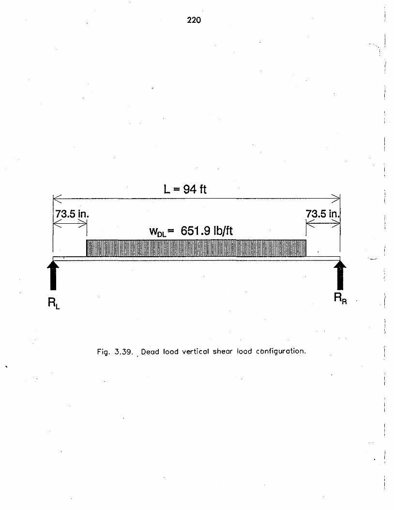
220
L=94ft
WoL = 651.9 lb/ft
'-..:.,.··
Fig. 3.39 .. Dead load vertical shear load cbnfiguration.

221
L = 94 ft
18.38 ft 14 ft 14 ft 47.82 ft
16 k 16 k 4k
I .
Fig, 3.40. Live lood verticol sheor lood configuration,
! '-

222
9. Determine bear:iJJg length and bear:iJJg suess. The allowable compressive stress perpendicular
to the grain, F.:, is computed as:
F .: = F ~ C.. = 650 psi (0.53) = 344.5 psi
The reaction due to a uniform dead load is:
R - WDL L - (651.9 lb/ft)(94 ft) - 30 639lbs DL____ - ' •
2 2
The distn1mtion factor for reactions is 1.00.
The reaction due to one wheel line may be found in Appendix A of the AASHTO
specifications (2).
For a 94 ft span multiplied by the distnoution factor:
Ru. = (1.00)(32,430 lb.) = 32,430 lbs.
The total reaction is then:
R.o.,1 = RoL + Ru. = 30,639 + 32,430 = 63,069 lbs.
The req ilired bearing length is computed as:
L = R_i = 63,069 lb. = 14.94 in. ,_,.,./, b F,L (12.25 in.)(344.5 lb/in2)
For. ease of constructiorr, use a bearing length of 18 in.
The reaction force shouid be recomputed based on the length of bearing:
.. tt ~- , .. ~ (651.9 lb/ft)(94 ft+ IU m./ '"'-)
2 RDL = ---------- = 31, 128 lbs.
?
The total reaction must also be recomputed:
R.o.,1 = RoL + Ru. = 31,128 + 32,430 = 63,558 lbs.
The total compressive stress at the bearing IS computed:
I. - 63,558 lb - 286 03 . u - (12.25 in.)(18 in.) - • PSI
The actual compressive stress is less than the allowable value, so the bridge is adequate with
respect to bearing.
10. Dctermlne camber. The dead load deflection is computed from:
A _ 5wL4
DL- 384E1 l •

'
223
!;, DL = 5(651.90)((94 ft)(12 inlfi)]'4 = 1.88 ill. (384)(1.499x 10S psi)(405,338 in4)(12 inlfi)
For a span length greater than 50 ft, use a camber of 2.0 times AoL·
Camber = 2.0(1.88) = 3.76 in. -> use 3.80 in.
SummaryofDesign Values
Geometry and design loadings:
Bridge length, L = 94.0 ft
Roadway width, W, = 24.0 ft
Design live load = HS20-44
Beam combination symbol: 24F-V4, Western species
Type of wearing surface: 3.00 in. asphalt
Beam dimensions and properties:
Beam width, b = 1214 in.
Beam depth, d = 73Y2 in.
Beam spacing, s = 5.00 ft
Beam section modulus, S, = 11,030 in.'
Beam cross sectional area, A = 900.37 in.2
Beam moment of inertia, I, = 405,338 in.'
Self weight of beam, w,,..m = 312.63 lb/ft
Stresses and deflections:
Actual bending stress, f, = 1554 psi
Allowable bending stress, F> = 1570 psi
Actual shear stress, f,, = 78 psi
Allowable shear stress, F., = 144 psi
Actual bearing stress, f... = 286 psi
Allowable bearing stress, F .. .' = 345 psi
Live load deflection, Au. = 1.68 in.
Allowable live load deflection "' 3.13 in.
Dead load deflection, b.oL = 1.88 in.
Design camber = 3. 75 in.
3.7.11. otue I aminated Panel Deck Bridge
3.7.11.1: Background
Longitudinal glulam timber deck bridges consist of a series of glulam panels spanning in the
~. direction of traffic and placed edge to edge across the deck width (see Fig. 3.41). A glulam panel deck is

224
< ~Bridge
Wearin surface
Stiffener beam Glulam anel deck
Fig. 3.41. Typical section of glulom timber deck bridge.

! \ ...
225
able to span up to 35 ft and can be used for either single- or multiple-lane bridges. The panels are usually
not connected, however, transverse stiffener beams are bolted below the deck to transfer loads between
panels (66).
Deck panels for longitudinal glulam bridges are designed as individual rectangular glulam beams.
The portion of the design vehicle live l?ad distribution to each panel is computed as a wheel load fraction
(WLF), which is very similar to the distnbution factor used for beam design. It is assumed that the entire
deck panel is effective in resisting applied loads.
The prefabrication of these panels allows for the pressure treatment of all laminates, which
significantly extends the service life of the bridge, and greatly simplifies construction
3. 7.11.2. Design Criteria
The design procedures discussed in this section are based on the AASHTO standard specifications
(2) and on research performed at ISU (69, 96, 97). The material and engineering properties for the glulam
deck bridge are ~om AITC 117 - Design (4).
3.7.11.3. Design Procedure
Spreadsheet input parameters refer to the spreadsheet in Fig. 3.42.
1. Define decll: geometric requiremenll and design loads. The effective span length, L, measured
from center-to-center of bearings, and bridge deck width, W, measured from curb-to-curb plus
any additional width required for railings, etc., must be determined. The design live loading
and timber species must also be specified (Input A, B, C and D). If an asphalt wearing surface
is to be used, it must be specified and thickness given (Input E and F).
2. Eadm.ate panel dlmensiona and IXllllpute section propertlea (Input G and H). Initially, an
estimate of the deck thickness and panel width must be made. For economy, the designer
should use a standard glulam dimension for deck thickness whenever. possible. Panel widths,
wP, are usually 42 to 54 in. in multiples of l'h in. for western species and H°' t:. for Southern
Pine. Table 3.33 may be used in estimating the required deck thickness for HS20-44 live
loading. The user must input the necessary parameters (Input G and H) and the spreadsheet
automatically performs the remaining calculations.
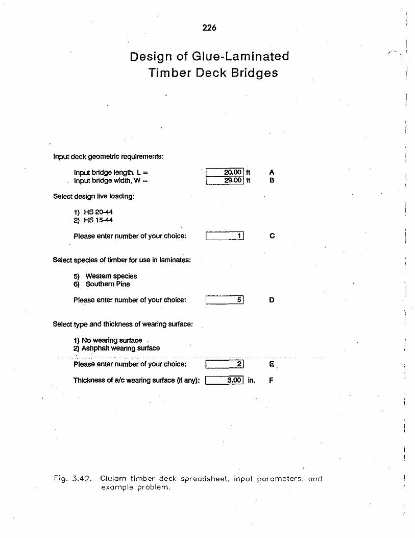
226
Design of Glue-Laminated Timber Deck Bridges
Input deck geometric requirements:
Input bridge length, L = 20.001 ft A Input bridge width, W = 29.00 ft B
Select design live loading:
1) HS20-44 2) HS 15-44
Please enter number of your choice: 11 c
Select species of timber for use in laminates:
5) Western species 6) Southern Pine
Please enter number of your choice: sl D
Select type and. thickness of wearing surface:
1) No wearing surface . 2) Ashphalt wearing surface
Please enter number of your choice: 21 E
Thickness of ate wearing surface flf any): 3.001 in. F
Fig. 3.42. Glulom timber deck spreadsheet, input parameters, and example problem.
...... ._

227
Input deck panel dimensions and computed section properties:
·~;.)• Initial est. of deck thickness, td = 10.750! in. G (based on span length}
Input panel width, wp = 49.50! In. H
Panel area, A= 532.13 in"2 Panel section modulus, Sy = 953.39 in"3 Panel moment of inertia, ly = 5124.47 in"4
Computed panel dead load and dead load moment:
Dead load of timber deck = 184.8 lbs/ft Dead load of wearing surface = 154.7 lbs/ft Railing load ;= 20.0 lbs/ft . Stiffener beam and hardware load = 8.0 lbs/ft Total design dead load = 367.5 lbs/ft
Design dead load moment, MDL = 18.37 ft-kips .
Computed wheel load fraction and live load moment:
Wheel load fraction, WLF = 0.924 Max. moment due to one wheel line = 80.00 ft-kips
Design live load moment, MLL = 73.92 ft-kips
Computed design moment, MT= (MDL+MLL) = 92.29 ft-kips
Computed design deck bending stress, lb = 1.16 ksi
Select deck combination symbol and computed allowable stress:
1) #2 • western species 2) #48 - southern pine
Please enter number of your choice: 11 Tabulated allowable bending stress, Fb = 1800 psi
(_ ... · Fig. 3.42. Continued.

Size factor for depth of members, CF = Allowable Bending stress, Fb' =
Computed check of live load deflection:
228
1.010
1.45 ksi
Deck is sufficient in flexure.
Adjusted modulus of elasticity, E' = 1.42E+06 ksi
Wheel line deflection, DELTAWL = 0.64 in.
Adjusted live load deflection, DELTALL = 0.59 in.
Allowable live load deflection = l/400 = 0.6 In.
Check DELTAL <allowable deflection? Deck is sufficient for deflection.
Computed check of horizontal shear:
Dead load vertical shear, VOL =
Compute LL vertical shear at distance =
Vertical shear due to one wheel line = Live load vertical shear, VLL =
Horizontal shear, V =
Horizontal shear stress, IV = Allowable shear stress, Fv =
Fig. 3.42. Continued.
3345 lb.
2.69 ft.
16,500 lb.
15,246 lb.
18,591 lb.
52.41 psi
126.88 psi
Deck is sufficient for shear.

229
Input stiffener material and computed configuration:
Select stiffener material:
1) Steel rolled section 2) Douglas fir-larch (sawn) 3) Hem-fir (north) (sawn) 4) Red pine (sawn) 5) Eastern white pine (sawn) 6) Southern pine (sawn)
Please enter number of your choice: el J
Preliminary stiffener spacing = 6.67 fl
Young's modulus, Estiff = 1,700 ksi
Moment of inertia req'd =
Input bearing width and computed bearing stress:
Input width of abutments, in: 121 in. K
WLF for reactions, WLFR = 1.031
LL reaction/wheel line, RWL = 20.80 kips
Live load reaction, ALL = 21.45 kips
Dead load reaction, RDL = 3.86 kips
Bearing stress, fcp = 42.61 psi
Allowable bearing stress, Fcp' = 296.8 psi
Deck is sufficient for bearing.
( '-~- Fig. 3.42. Continued.

230
Summary of Design Values
Geometry and dimensions:
Length, L = 20.00 ft
Width, w = 29.00 ft
Design live loading: AASHTO HS20
Timber species: Western species
Deck combination symbol: #2 ·Western species
Thickness of deck, td = 10.75 in.
Wearing surface: Asphalt
Thickness of wearing surface : 3.00 in.
Stresses and deflections:
Bending stress, fb = 1.16 ksi
Allowable bending stress, Fb' = 1.45 ksi ! I
Horizontal shear stress, fv = 52.41 psi
Allowable shear stress, Fv = 126.88 psi
Bearing stress at abutment = 42.61 psi
Allowable bearing stress, Fcp' = 296.8 psi
Live load deflection, deltaL = 0.59 in.
Allowable LL deflection, L/400 = 0.60 in.
Fi9. 3.42. Continued.
: I

231
Table 3.33. Glulam timber deck thicknesses and span lengths.
Deck Simple Continuous thickness span span
(in.) (ft) (ft)
5 or 51As 6 7
6'.4 10 12
8'h or 8¥. 15 18 .
lO'h or 103.4 21 23
1214 24 27
1414 27 31
Based on an estimated panel size, the section properties for the section can be computed:
w, = panel width (in.)
t,. = panel thickness (in.)
A = panel cross sectional area (in2)"" w,t
Sy = section modulus of panel (in3) =
ly = moment of inertia of panel (in') =
2 Wptd
6
3 wPt4
12
3. Compute panel dead load. The uniform panel dead load of the deck and wearing surface can
be computed using the following unit weights:
• timber (treated or untreated) = 50 lb/ft3
• asphalt or concrete = 150 lb/ft3
The spreadsheet performs this calculation automatically using input parameters E and F which
were input in design step 1.
Table 3.34 may be .used for estimating the dead load of the timber deck plus a 3 in.
asphalt or concre.te wearing surface.
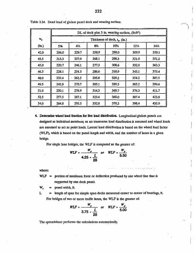
232
Table 3.34. Dead load of glulam panel deck and wearing surface.
DL of deck plus 3 in. wearing surface, (lb/ft3)
w, Thickness of deck, i,,, (in.)
(in.) S'Ai 6'1. 8:Y. 1()3;. 1214 1414
42.0 206.0 229.7 258.9 288.0 309.9 339.1
43.5 213.3 237.9 268.1 298.3 321.0 351.2
45.0 220.7 246.1 277.3 308.6 332.0 363.3
46.5 228.1 254.3 286.6 318.9 343.1 375.4
48.0 235.4 262.5 295.8 329.2 354.2 387.5
49.5 242.8 270.7 305.1 339.5 365.2 399.6
51.0 250.1 278.9 314.3 349.7 376.3 411.7
52.5 257.5 287.1 323.6 360.0 387.4 423.8
54.0 264.8 295.3 332.8 370.3 398.4 435.9
4. Dctermlne wheel )Qad fraclion for live IQad d1'ltrlbution. Longitudinal glulam panels are
designed as individual members; as no transverse load distnoution is assumed and wheel loads
are assumed to act as point loads. Lateral load diStnoution is based on the wheel load factor
(WLF), which is based on the panel length and width, and the number of lanes in a given
bridge.
For single lane bridges, the WLF is computed as the greater of:
WLF = W or WLF = _!!£_ 4.25 + :a 5
•50
where:
WLF = portion of maximum force or deflection produced by one wheel line that is
supported by one deck paneL
w, = panel width, fl
L = length of span for simple span decks measured center to center of bearings, fl
For bridges of two or more traffic lanes, the WLF is the greater of:
w w WLF = or WLF = ...:.:..L
3.75 + _f_ 5·00 28
The spreadsheet performs the calculations automatically.
,- ' \

i
233
S. Detennlne dead load and liYC load moment The panel dead load moment can be computed
based on the uniform dead load, w01, previously determined:
The live load moment, Mu.. is computed by multiplying the maximum moment for one
wheel line of the design vehicle by the WLF:
where:
Mu. = live load moment applied to one panel, in-lb.
MWL = maximum moment produced by one wheel line of the design vehicle, in-lb.
Conservatively, the maximum dead load moment and maximum live load moment can be
added, even though the occur at different positions along the span.
The total design moment, MT, is the sum of the maximum live and dead load moments:
The spreadsheet computes this step automatically based on the span length and design vehicle
chosen.
6. Compute bending stress and select combination symboL The deck bending stress, f., computed
as the design moment divided by the panel section modulus, Sy, cannot exceed the allowable
bending stress adjusted for wet use and size factors:
where:
F.' = F,,,. CM Cp
F,,,. = tabulated bending stress for species of interest
= 1800 lb/in.2 for Western Species
= 1750 lb/in.2 for Southern Pine

234
I
C.. = wet use factor for glulam = 0.80
Cp = size factor for thin panels (see Table 3.35)
If the calculated flexural stress exceeds the allowable value computed above, either the
deck thickness, t,,, must be increased, or a higher grade of lumber (one with better material
properties) must be utilized. If f,, is significantly less than the allowable stress value, a thinner
deck or a lower-grade material may be used. No changes should be made until the live load
deflection is reviewed.
The user must select a combination symbol (Input I) and the spreadsheet will perform
the remaining calculations.
7. Cleek live load deflection. The live load deflection, Au.. is a function of the panel moment of
inertia and is produced by one wheel line of the design vehicle times the WLF:
where:
ALL = live load panel deflection, in.
AWL = maximum live load deflection produced by one wheel line of the design vehicle, in.
Table 3.35. Size factor for glulam timber deck panels.
t (in.) Cp
Sor S'Ai 1.10
@h 1.07
8'1i or 8* 1.04
lO>i or 10* 1.01
The deck live load deflection can be computed by standard elastic analyses, using the
glulam modulus of elasticity adjusted for wet-use conditions. For a uniform load, the live load
deflection can be found from:
5w L4 A - u.
u - 384E1 I
l i~,1 \.

235
AASHTO specifications do not limit live load deflection for glulam timber decks, thus
the allowable deflection is left to the designer. Recommended practice limits maximum
deflection to U360.
The spreadsheet performs this calculation and compares the result to the allowable
value.
8. Qedt horizontal shear. Because of the relatively large panel area, horizontal shear is rarely a
controlling factor; however, it should be checked. Horizontal shear (i.e. vertical shear) due to
dead and live load is assumed to be resisted by the total area of the deck paneL
The dead toad vertical shear is computed at a distance from the support equal to the
thickness, I, and is given by:
where:
VoL = dead load vertical. shear (lb)
w0L = uniform panel dead load (lb/ft)
The live load vertical shear is computed at a distance from the support equal to the
lesser of 3 times the deck thickness (3t) or the span quarter point (U4), and is equal to the
maximum shear due to one design wheel line times the WLF.
where:
Vu. = live toad vertical shear (lb)
VWL = max. vertical shear produced by one wheel line (lb)
The applied shear stress must not exceed the allowable shear stress for the deck
combination symbol, given by:
where:
V = VoL + Vu.. lb.
A = panel cross-sectional area, in'.

236
C.. = wet-use factor for shear = 0.875.
The maximum dead and live load shear do not occur at the same position along the
span, can be combined for simplicity. When(, > Fv', the only alternatives for the designer are
to increase the deck thickness or panel width. In either case, the design procedure must be
recycled. The spreadsheet performs this step automatically.
9. Determine atfffener spacing and configuration. Transverse stiffener beams typically consist of
horizontal glulam beams or shallow rolled steel sections, and are intended to distn'l>ute loads to
adjacent panels. The design criteria for transverse siiffener beams is based on research done at
ISU. Stiffener beams are often used for guardrail post attachment, so rail loads and connection
details must also be considered.
AASHTO specifications require that a transverse stiffener beam be placed at midspan
for all deck span lengths, and at intermediate spacings of s 10 ft. An intermediate spacing of 8
ft, recommended by AITC, will be used in the subsequent design.
The empirical stiffener design requires that the transverse stiffener has a bending
stiffness, E'I, of :i: 80,000 k-in2. Note that transverse load distn'l>ution between panels is
influenced more by stiffener spacing than by the bending stiffness, E'I.
The connection between the stiffener and the deck panels depends on the type of
stiffener beams used. A bolt may be placed through the deck and stiffener for both glulam
beams and steel channel sections. Deck brackets or steel plates may be used for glulam beams
and C-type clips may be used to connect the top flange of a rolled section.
10. Determine bearing configuration and c:heck bearing
lltrCllL For longitudinal deck bridges, the required bearing area is usually controlled by the
required configuration, rather than compressive stresses. A bearing length of 10 to 12 in. is
recommended for stability and simplicity.
The dead load reaction for a glulam deck bridge can be computed using the unit dead
load of the panel The live load reaction is based on a wheel load factor of W p/4, but not less
than 1.0. The live load reaction distn'buted to each panel is the maximum reaction for the
design vehicle, multiplied by the WLF.
The bearing stress due to RDL and RlL must not exceed the allowable value for the panel
being used. This may be expressed as:

i ·~
237
where i. is the length of the panel bearing in inches.
3. 7.11.4. Example
An existing bridge is to be replaced with a longitudinal glulam deck bridge. The replacement bridge
must have a 20 ft span from center-to-eenter of bearings, a roadway width of 26 ft, and must support two
lanes of AASHTO HS20 live loading-, The spreadsheet input and output for this example is shown in Fig.
3.42.
L Define deck gcomctty and design loads. The bridge span length, L, must be determined.
(Input A). ·Bridge width must consider the roadway width, 26 ft, and the curb and railing on
each side:
W = 26 ft+ 2 ft+ 2(6 in.)= 29 ft. (InputB)
Design live load = one HS-20 wheel line. (Input C)
The designer specifies the species of timber to be used in the laminates. Most common
for glulam deck.bridges are western species and Southern Pine. For this example western
species are selected. (Input D)
The designer must specify if a wearing surface is going to be used for the proposed
bridge; if used its thickness needs to be given. For this example, a 3.0 in. asphalt wearing
surface is selected. (Input E and F)
2. Estimate panel size and compute section properllea. From Table 3.33, select an initial deck
thickness of 10'.4 in. (Input G) The panel width must be 42 to 54 in., in 1 'h in. increments. For
this example, select two 51 in .. wide panels, and five panels 491h in. wide, for a total width of 29
ft·l'h in. (InputH). The section properties for the 491!2 in. panel will be conservatively used
for all panels.
Section properties for this panel can be computed as:
t = 10.75 in.
w, = 49.5 in.
A = w, t = 10.75(49.5) = 532.13 in2
S = w, t2 = (49.5 in.)(10.75 in.)2 = 953.39 tn3 1 6 6
1 = w,. t3 = (49.5 in.)(10.75 in.)3 = 5124.47 in4 1 12 12
3. Compute panel dead load and dead load moment. From Table 3.34, the dead load of a 49.5 in.
panel with a 3 in. asphalt wearing surface can be determined as:

238
WoL = 339.5 lb/ft.
The dead load due to the railing is assumed to be distnbuted equally over the entire
deck. The dead load due to the railing is:
w ... m., = 2(55 lb/ft)(l panels = 15.7 lb/ft.
A conservative estimate of 20 lb/ft has been assumed for the railing load in the remaining
calculations. An additional 8 lb/ft should be added to account for stiffener beams and railing
hardware.
wllllpo.., = 339.S + 20 + 8 = 367.S lb/ft.
The dead load moment is computed by:
MoL = (367.5 lb/ft/!000)(20 ft)2 = 18.37 ft-k
4. Determine wheel load fracdon for live load clistributlon. For a two Jane bridge, the wheel load
fraction can be determined as the larger of the following:
WLF = 49.5 in./12 = 0.83 WL µr /iaMl 5.00
For this example, use WLF = 0.924 WIJpaneL
5. Determine dead load and live load moment. The maximum live load moment due to one
wheel line can be found in Appendix A, AASIITO (2). For the 20 ft span of this example, ·
M.t...t ""' = 80,000 ft-lb. The live toad moment distnbuted to each panel is given by:
MLL = (0.924 WIJpanel)(80 ft k) = 73.92 ft-k
The total design moment, MT can be computed as:
MT = MoL + MLL = 18.37 + 73.92 = 92.29 ft-k
Note, although the maximum dead load and live toad moments do not occur at the same
point along the span, they can conservatively be added for simplicity.
6. Compute bending stress and select combination symboL The bending stress in the deck is:
/, = 92.29ft-k(12) =1.16ksi b 953.39 in3
The deck combination symbol chosen for this example is a No. 2 (Input I).
/· ... I

239
The design properties can be found in AITC 117 ( 4):
F.,. = 1800 psi CM = 0.80
F., = 145 psi 41 = 0.875
F.,_ = 560 psi
E = 1.7 x 10⁶ psi
CM= 0.53
CM= 0.833
For the deck thickness which has been chosen, the size factor, Cp = 1.01.
The allowable bending stress for the chosen combination symbol is given by:
F> = F., 41 Cp = (1800 psi)(l.01 )(0.80) = 1.45 ksi
The actual bending stress is less than the allowable value, so the deck is adequate in
flexure.
7. 01eck liYe load deflectlon. The deflection coefficient for one line of HS20 wheels can be
obtained from simple engineering mechanics or a tabulated value can be used (Table 16-8, Ref.
66). For the 20 ft span in this example the deflection coefficient = 4.61 x 10⁹.
A. - 4.61 :x: 109 WL- 'E1 l
J
E' = E CM = (1.7 x 10⁶)(0.833) = 1.416 x 10⁶ lb/in.2
ti. = 4.61 :x: 109 = O.S4 in. WL (1.416;x; 108)(5124.47)
The deck deflection can then be computed as:
A.LL = A.WL WLF = (0.64 in.)(0.93) = 0.60 in.
The allowable live load deflection is L/400 = 0.60 in. The deck is thus sufficient for live
load deflection,
8. 01eck horlwn1lll shear. The dead load vertical shear is computed at a distance t from the
support:
VDL = (367.5 lb/ft)(~ -10.75ft) = 3345 lb. . 2 12
The live load vertical shear is computed at a distance of 3t or L/4, which ever is less.
For this example:
3t = 3(10.75 in.)/12 = 2.69 ft
1./4 = 20 ft/4 = 5 ft
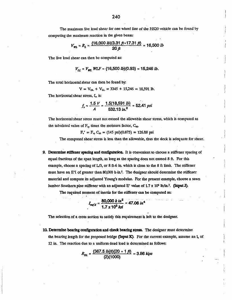
240
Tue maximum live load shear for one wheel line of the HS20 vehicle can be found by
computing the maximum reaction in the given beam:
VWl." RL = (16,000 lb)(3.31 ft+17.31 ft) = 16,500 lb 20/t
The live load shear can then be computed as:
Vu= VWL WLF = (16,500 lb)(0.93) = 15,246 lb.
The total horizontal shear can then be found by:
V = VoL +Vu.= 3345 + 15,246 = 18,591 lb.
The horizontal shear stress, f., is:
!. = 1.5 v = 1.5(18,591 lb) = 52.41 si • A 532.13 in.2 P
The horizontal shear stress must not exceed the allowable shear stress, which is computed as
the tabulated value of F.,. times the moisture factor, C,..
Fv' = F.,. C,. = (145 psi)(0.875) = 126.88 psi
Tue computed shear stress is less than the allowable, thus the deck is adequate for shear.
9. Dclemlfne stiffener apadll& and conflgmatlon. It is convenient to choose a stiffener spacing of
equal fractions of the span length, as long as the spacing does not exceed 8 ft. For this
example, choose a spacing of L/3, or 8 ft-6 in. which is close to the 8 ft limit. The stiffener
must have an E'l of greater than.80,000 k-in.2. The designer should determine the stiffener
material and compute its adjusted Young's modulus. For the present example, choose a sawn
lumber Southern pine stiffener with an adjusted E' value of 1.7 x 10' lb/in.2• (InputJ).
The required moment of inertia for the stiffener can be computed as:
l = 80,000 k in2 = 47.06 m• .,_.,, 1.7x10³tw
The selection.of a cross section to satisfy this requirement is left to the designer.
10. Determine bearing conflgmation and check bearing stress. The designer must determine
the bearing length for the proposed bridge (Input K). For the current example, assume an !,, of
12 in. The reaction due to a uniform dead load is determined as follows:
R = (367 .5 lb[ft)(20 + 1 ft) = 3 B6 ""'"" DL (2)(1000) • "'I"'

·.,~.,.'
241
The live load reaction is computed as the maximum reaction due to one wheel line of
the design vehicle times the WLF.
WLF- = ~ = 4·13.ft = 1.031 WL/PQMl .4 4
The maximum reaction for a 20 ft span due to an HS20 loading, Rwu is 20,800 lbs. (Appendix
A, AASHTO (4)). The live load reaction is then:
Ru. = RWL WLF = (20.80 kips)(l.031) = 21.45 kips
For a bearing length of 12 in., the compressive stress perpendicular to the grain, F.,,, is
computed as:
f, - 3.86 + 21.45 - 42 61 . .... - (1000)(49.5)(12) - . psi
The actual bearing stress must be less than the allowable value, which is computed by:
F.,,' = F.,, CM = (5(,() psi)(0.53) = 296.8 psi
The stress is less than the allowable value, so the deck is adequate for bearing.
Summa!y of design values:
Geometry and loading:
Length, L = .20.00 ft
Width of roadway, W = 26.00 ft
Design live load: AASHTO HS20
Timber species: Western Species
Deck combination symbol: No. 2 - Western Species
Deck thickness, t,, = lCH~ in.
Wearing surface: 3 in. asphalt overlay
· Stresses and deflections:
Bending siress, r. = 1.16 ksi
Allowable bending stress, F,' = 1.45 ksi
Horizontal shear stress, f. = 52.41 psi
Allowable shear stress, F. = .126.88 psi
Bearing stress at abutment, Cu = 42.61 psi
Allowable bearing stress, F.,..' = 296.8 psi
Live load deflection, ~ u. = 0.(i() in.
Allowable live load deflection, U400 = 0.(i() in.

245
4. SUMMARY AND CONCLUSIONS
4.1. Summary
The major emphasis of this study was to develop a manual to assist the county engineer in making cost
effective bridge strengthening and replacement decisions. The study was performed in two phases; 1) the
determination and prioritiz.ation of criti<:al problems on Iowa's Secondary bridge system and 2) development
of solutions for the problems identified in Phase 1.
The two bridge types with the greatest needs and greatest potential for strengthening are FHW A Type
302 (steel stringer) and Ff!WA Type 702 (timber stringer) bridges. Methods presented for strengthening the
steel stringer bridges include (1) replacement of damaged stringers, (2) respacing existing stringers and adding
stringers, (3} increasing the section modulus of existing stringers, (4) developing composite action, (5) replacing
existing deck with a lightweight deck, and (6) post-tensioning. For timber stringer bridges, the following
methods are included: (1) res pacing existing stringers and adding timber stringers, and (2) adding new steel
stringers. Each of these procedures are explained and, where applicable, examples are provided.
Microcomputer spreadsheets have been developed for items (1), (2), (3) and (6) above for steel stringer bridges
and for item (1) above for timber stringer bridges.
Replacement methods for low volume road applications have also been included in tile manual Some
of the methods presented are proprietary. Where appropriate, design examples and cost info~ation has been
provided. The following bridge replacement types are included (1) precast culvert/bridge, (2) air formed arch
culvert, (3) welded steel truss bridge, ( 4) prestressed concrete beam bridge, (5) Inverset bridge system, (6)
precast multiple tee beam bridge, (7) low water stream crossing, (8) corrugated metal pipe culvert, (9) stress
laminated timber bridge, (10) glue-laminated timber beam bridge, and (11) glue-laminated panel deck bridge.
Microcomputer spreadsheets have been developed for items (9), (10) and (11) above.
For determining the cost effectiveness of each of the methods of strengthening and replacement, a
method of economic analysis (equivalent uniform annual cost) as well as cost data have been presented. This
allows the engineer to select the most appropriate alternative: (1) replacing the existing bridge or (2)
strengthening the existing bridge. The economic model developed allows each alternative to be quantified so
that each can be compared in a rational manner.
Information related to inspection of bridges is included in this manual Before an accurate evaluation
of a bridge can be performed, it is imperative that a thorough inspection be performed. Fundamentals related
to evaluation of a bridge are also included in the manual
4.2. Conc:luslona 1. Steel stringer and timber stringer bridges are the bridge types on the. secondary road system in Iowa
with greatest potential for cost-effective strengthening methods.
2 Coun~engineers' requests for design aids to assist them in evaluation, strengthening and replacement
decisions have been provided.

3.
246
Numerous strengthening procedures have been provided for the two types of bridges (steel stringer
and timber stringer) with the greatest potential for strengthening.
4. In situations where strengthening is not cost effective, information has been provided on numerous
replacement structures.
I '"'·
247
S. ACKNOWLEDGMENTS
. . . The study presented in this report was conducted by the Bridge Engineering Center under the auspices
of the Engineering Research Institute of Iowa State University. The research was sponsored by the Iowa
Department of Transportation and the Iowa Highway Research Board under Research Project HR-323 . . r
Special thanks are accorded B. T. Shivakumar, graduate student in Structural Engineering, and Theresa
Connor, undergraduate student in Civil Engineering for their help with the study. Denise Wood, secretary for
Structural Engineering, is given special recognition for her superior efforts in typing the report manuscript
The input of several Iowa DOT employees is gratefully acknowledged, most significantly Larry Jesse
and othen; at the Office of Local Systems. The input provided by the advisory panel identified in Sec. 2.1 of
the report is gratefully acknowledged.
Gordon Burns, who served as subcontractor for portions of this study is thanked for his valuable
contnl>ution to Secs. 3.2 and 3.3 of Chp. 3 of this report

249
6. REFERENCES
1. American Association of State Highway and Transportation Officials, Guide Specifications for the Design ofStresS-Laminated Wood Decks, AASHTO, Washington, D.C., April 1991, 12 pp.
2. American Association of State Highway and Transportation Officials, Standard Specification for Highway Bridges, AASHTO, Washington, D.C., 1989, 420 pp.
3. American Association of State Highway and Transportation Officials, Manual for Maintenance Inspection of Bridges, AASHTO, Washington, D.C., 1979.
4. American Institute of Timber Construction, Design Standard Specifications for Structural Glued Laminated Timber of Softwood Species, AITC 117-87-Design, Englewood, CO, 1987, 28 pp.
S. American Institute of Timber Construction. Timber C-Onstruction Manual, 3rd ed. John Wiley and Sons, Inc., New York, 1985, 836 pp.
6. American Institute of Steel Construction, Manual of Steel C-Onstruction, Allowable StresS Design, AISC, Ninth Edition, Chicago, Ill, 1989.
7. Applied Technology Council (ATq, 'Seismic Retrofitting Guidelines for Highway Bridges.• Federal Highway Administration, Final Report, Repon No. FHWA-RD-83.()()7 (Dec. 1983), 219 pp.
8. Batchelor, B. E., 'Relaxation Characteristics of Prestressed Laminated Wood Decks.• OJT and CRP Report 23123, Queen's University, Kingston, ON, Canada, 1981.
9. Batchelor, B., Van Dalen, K., Morrison, T., and Taylor, R. J., 'Structural Characteristics of Red Pine and Hem-F"ir in Prestressed Laminated Wood Bridge Decks.• Queen's UnivetSity, Report 23122, Kingston, ON, Canada, 1981.
10. Berger, R. H., "Extending the Service Life of Existing Bridges by Increasing Their Load Carrying Capacity.• RlWA Repon No. FHWA-RD-78-133 (Jun. 1978), 75 pp.
11. Besser, D. M., 'Secondary System Bridge Problems and Strengthening Solutions', M.S. Thesis, Iowa State University, Ames, IA (May 1993), 93 pp.
12. Brungraber, R., Gutkowski, R., Kindya, W. and McWilliams, R., "l'imber Bridges: Part of the Solution for Rural America.• TRB Record 1106, Transportation Research Board, 1987, pp. 131-139.
13. Cady, P. D. 'Bridge Deck Rehabilitation Decision Making', TRB Record 1035, Transportation Research Board (1985), pp. 13-20.
14. Cady, P. D., "Inflation and Highway Economic Analysis•, ASCE, Journal of Transportation Engineering, VoL 109, No •. S (Sept. 1983), pp. 631-639.
15. Cook, J. P., "!'he Shear Connector', C-Omposite C-Onstruction Methods, John Wiley and Sons, N.Y. (1977), pp. 168-172.
16. Cooper, James, D., "A New Era in Bridge Engineering Research', Proceedings of the Second Workshop on Bridge Engineering Research iD Progress, Reno, Nevada (Oct. 1990), pp. 5-10.
17. "County takes new approach to building short span bridges•, C-Onstruction Digest (Aug. 1990), pp. 34-36.

250
18. Crow, E. L, Davis, F. A, and Maxfield, M. W., Statistics Manuai Dover Publications, Inc., New York, (1960), pp. 87-88.
19. Dallam, L N., •static and Fatigue Properties of High-Strength Bolt Shear Connectors•, Missouri Cooperative Highway Research Program Report 7()..2, Engineering Experiment Station, University of Missouri-Columbia (1970), 49 pp.
20. Dallam, L N., •Pushout Tests with High-Strength Bolt Shear Connectors•, Missouri Cooperative Highway Research Program Report 68-7, Engineering Experiment Station, University of MissouriColumbia (1968), 66 pp.
21. Dedic, D. J., and Klaiber, F. W., •High Strength Bolts as Shear Connectors in Rehabilitation Work', Concrete International: Design and Constiuction, Vol 6, No. 7 (July 1984), pp. 41-46.
22. Dunker, K. F., Klaiber, F. W., Daoud, F. W., Wiley, W. E., and sanders, W. W., Jr., "Strengthening of Existing Composite Bridges•, Iowa Department of Transportation Project HR-287, ISU-ERI-Ames-88007, Iowa State University, Ames, Iowa (July 1987), 220 pp.·
23. Dunker, K. F., Klaiber, F. W., Beck, B. L, and Sanders, W. W., Jr., •strengthening of Existing Single Span Steel Beam and Concrete Deck Bridges•, Final Report-Part II, Iowa Department of Transportation Project HR-238, ISU-ERI-Ames-85231, Iowa State University, Ames, Iowa (March 1985), 146 pp.
24. Dunker, K. F., Klaiber, F. W., and Sanders, W. W., Jr., •0esign Manualfor Strengthening Single-Span Composite Bridges by Post-Tensioning", Final Report - Part III, Iowa Department of Transportation Project HR-238, ISU-ERI-Ames-85229, Iowa State University, Ames, Iowa (July 1985), 102 pp.
25. FHW A Office of Engineering, Bridge Division, Recording and Coding Guide for tbe Structure Inventory and Appraisal of tbe Nation's Bridges, Federal Highway Administration (Dec. 1988), 126 pp.
26. Fisher, J. W., Hausamann, H., Sullivan, M. D., and Pense, A W., "Detection and Repair of Fatigue Damage in Welded Highway Bridges•, NCHRP Report 206 (Jun. 1979), 85 pp.
27. Galambos, C. F., •Bridge Design, Maintenance, and Management', Public Roads, 50, No. 4 (March 1987), pp. 109-115.
28. Gangarao, H. V. S. and Zelina, T. R., "Development of Economical Low-Volume Road Bridges", AS~ Journal of Structural Engineering, Vol 114, No. 9 (Sept. 1988), pp. 1941-1961.
29. Gangarao, H. V. S., Ward, R., and Howser, V., "Value Engineering Approach to Low-Volume Road Bridge Selection·, AS~ Journal of Structural Engineering, V. 114, No. 9 (Sept. 1988), pp. 1962-1977.
30. Gangarao, H. V. and Hegarty, M. J., •Developments of New Design and Construction Guidelines for Low-Volume Road Bridges•, TRB Record 1106, Transportation Research Board (1987), pp. 122-130.
31. Grossman, S. J., "Upside-Down Casting Combines Advantages of Steel and Concrete•, Modern Steel Construction, Vol 31, No. 3 (March 1991), pp. 23-25.
32. Heine, M., 'Welded Truss Bridges: Rural Road Remedy", Roads and Bridges (Nov. 1990), pp. 42-43.
33. Johnston, D. W. and Zia, P., "Level-of-Service System for Bridge Evaluation", TRB Record %2, Transportation Research Board (1984), pp. 1-8.
I

251
34. Kempter-Rossman International, "Value Engineering for Highways", Federal Highway Adminsitration, Washington, D.C. (1980), 111 pp.
35. Klaiber, F. W., Dunker, K. F., Planck, S. M. and Sanders, W. W., Jr., "Strengthening of an Existing Continuous.Span, Steel-Beam, Concrete-Deck Bridge by Post-Tensioning', Final Report, Iowa Department of Transportation Project HR-308, ISU-ERI·Ames-90210, Iowa State University, Ames, IA (Feb. 1990), 165 pp.
36. Klaiber, F. W., Dunker, K. F., Wipf, T. J. and Sanders, W.W., Jr., 'Methods of Strengthening Existing Highway Bridges', NCHRP293 (Sept 1987), 114 pp.
37. Klaiber, F. W., Dedic, D. J., Dunker, K. F. and Sanders, W.W., Jr., 'Strengthening of Existing Single Span Steel Beam and Concrete Deck Bridges by Post-Tensioning", Final Report-Part I, Iowa Department of Transportation Project HR-214, ISU-ERI·Ames-83135, Iowa State University, Ames, IA (Feb. 1983), 185 pp.
38. Klaiber, F. W., Dunker, K. F. and Sanders, W. W., Jr., 'Feasibility Study of Strengthening Existing Single Span Steel Beam Concrete Deck Bridges", Final Report, Iowa Department of Transportation Project HR-238, ISU-ERI-Ames~1251, Iowa State University, Ames, IA (June 1981), 141 pp.
39. Lapin, L., Probability and Statistics for Modem Engineering, Brooks/Cole Publishing Co., Belmont, CA (1983), pp. 59()..591.
40. La Violette, M. D., "Cost Effective Rehabilitation and Replacement of Low Volume Road Bridges', M.S. Thesis, Iowa State University, Ames, IA (May 1993), 291 pp.
41. Lemmerman, J. H., 'Quick Benefit-Cost Procedure for Evaluating Proposed Highway Projects", TRB Record 984, Transportation Research Board, pp. 11·22.
42. Lotus Development Corporation, User's Guide· Lotus 123 for DOS, Release 2.3, Lotus Development Corporation, Cambridge, MA, 1991.
43. Mancarti, G. D., 'Strengthening Short Span Bridges for Increased Live Loads', Proceedings of the Third International Conference on Short and Medium Span Bridges, Toronto, Ontario (Aug. 1990), pp. 169-180.
44. Mccutcheon, W. J., Gulko~ki, R. M and Moody, R. C., 'Performance and Rehabilitation of Timber Bridges', TRB Record 1053, Transportation Research Board (1986), pp. 65-69.
45. McFarland, W. F., Griffin, L. I., Rollins, J. B., Stockton, W. R., Phillips, D. T. and Dudek, C. L, "Assessment of Techniques for Cost-Effectiveness of Highway Accident Countermeasures", EfWA Report No. FHWA-RD-79-53 (Jan. 1979), 337 pp.
46. McLin, L, "County Produces Bridge Beams for Super Savings", Roads and Bridges (Nov. 1990), PP· 4041.
47. Mishler, H. W. and Leis, B. N., "EvaluationofRepairTechniquesfor Damaged Steel Bridge Members: Phase I', Final Report, NCHRP Project 12-17 (May 1981), 131. pp .
.;
<IS. Moses, F., "Evaluation of Bridge Safety and Remaining Life", Proceedings of the Structures Congress 1989 Conference, San Francisco, CA (May 1989), pp. 717-726.

252
49. Motayed, A. K., Chang, F. M. and Mukherjee, D. K., 'Design and Construction of Low Water Stream Crossing- Executive Summary•, FHWA Report No. FHWNRD-83/015 (Sept. 1983), 20 pp.
50. Mudge, A. E., Value Engineering: a systematic approach, McGraw-Hill, New York, NY, 1971.
51. National Forest Products Association, Design Values for Wood <:onstruction, NFP A (1986), 34 pp.
" ,.,
52. National Forest Products Association, Natidnal Design Specifications for Wood <:onstruction,National Forest Products Association, Washington, D.C. (1986), 87 pp.
53. Newnan, D. G., Efp.gineering Economic Analysis, 3rd ed. Engineering Press, San Jose, CA, 1988.
54. 'New Trusses Upgrade Ohio County Bridge•, Roads and Bridges (Nov. 1987), pp. 34-35.
55. Nilson, A. H., Design of Prestressed <:oncrete, 2nd edition, John Wiley and Sons, New York, NY (1987), 592 pp.
56. 'Ninth Annual Report to Congress - Highway Bridge Replacement and Rehabilitation Program", FHWA, Washington, D.C., 1989.
57. Oliva, M. G. and Dimakis, A., 'Behavior of Stress-laminated Timber Highway Bridge•, ASCE Structural Journal Vol 114, No. 8 (Aug. 1988), pp. 1850-1869.
58. Oliva, M. G., Tuomi, R. L. and Dimakas, A. G., 'New Ideas for Timber Bridges•, TRB Record 1053, Transportation Research Board (1986), pp. 59-65.
59. Park, S. H., Bridge Rehabilitation and Replacement (Bridge Repair Practice), S. H. Park, Trenton, New Jersey (1984), .818 pp.
60. PCI Design Handbook, 3rd edition, Prestressed Concrete Institute, Chicago, IL, 1985.
61. Petermeier, D., 'Bridge Management Systems•, M.S. Thesis, Iowa State University, Ames, IA (May 1991 ), 201 pp.
62. Prestressed Concrete Institute, Precast Prestressed <:oncrete Short Span Bridges - Spans to 100 Feet, Chicago, IL, 1st ed., 1975.
63. Prestressed Concrete Institute, Design Supplement to: Precast Prestressed <:oncrete Short Span Bridges - Spans to 100 Feet, Chicago, IL, 1984. ·
64. Reel, R. S. and Muruganandan, C., 'Use of Financial Analysis in Bridge Rehabilitation Projects in Ontario', Proceedings of the Tbird'lntemational OJnference on Short and Medium Span Bridges, Toronto, Ontario (Aug. 1990), pp. 53.02.
65. 'Replacing Rural Bridges•, Roads and Bridges (Nov 1985), pp. 51-53.
66. Ritter, M. A., Timber Bridges: Design, <:onstruction, Inspection, and Maintenance, U.S. Department of Agriculture, Forest Service, Washington, D.C. (1990), 944 pp.
67. 'Rural Bridges: An Assessment Based Upon the National Bridge Inventory', Transportation Report, United States Department of Agriculture, Office of Transportation, April, 1989.
68. Sabnis, G. M., "Innovative Methods of Upgrading Structurally and Geometrically Deficient Through Truss Bridges", FI-IWA, Report No. FHWA-RD-82-041 (Apr. 1983), 130 pp.

~·-···
I
69.
70.
71.
72.
73.
74.
75.
76.
77.·
78.
79.
80.
253
Sanders, W. W., Klaiber, F. W. and Wipf, T. J., "Load Distnllution in Glued Laminated Longitudinal Timber Deck Highway Bridges", Report ISU-ERI-AMES-85441, Iowa State University, Ames, IA (Aug. 1985), 47 pp.
Sarisley, E. F. and Accorsl, M. L., 'Prestress Level in Stress-laminated Timber Bridges•, ASCE, Structural Journal, VoL 116, No. 11 (Nov. 1990), pp. 3003-3019.
Shanafelt, G. 0. and Horn, W. B., "Guidelines for Evaluation and Repair of Prestressed Concrete Bridge Members", NCHRP Report 280 (Dec. 1985), 84 pp.
Shanafelt, G. 0. and Horn, W. B., 'Guidelines for Evaluation and Repair of Damaged Steel Bridge Members', NCHRP Report 271(Jun.1984), 64 pp.
Shanafelt, G. 0. and Horn, W. B., 'Damage Evaluation and Repair Methods for Prestressed Concrete Bridge Members", NCHRP Report 226 (Nov. 1980), 66 pp.
Shivakumar, B. T., •strengthening of Existing Tiinber Stringer Bridges by the Addition of Steel Stringers', M.S. Thesis, Iowa State University, Ames, IA (May 1992), 79 pp.
Smith, G. W., Engineering Economy: Analysis of Capital Expenditures, 3rd ed. Iowa State University Press, Ames, Iowa, 1979.
Sprinkle, M. M., "Prefabricated Bridge Elements and Systems', NCHRP Synthesis of Highway Practire 119 (Aug. 1985), 15 pp.
Sprinkle, M. M., "Final Report of Evaluation of the Performance of a Presslam Timber Bridge - Bridge Performance and Load Test afters Years•, Virginia Highway and Transportation Research Council Report VHTRC 82-RS6 (1982), 21 pp.
Sprinkle, M. M., 'Evaluation of the Performance of a Presslam Timber Highway Bridge'. Interim Report 2•, Virginia Highway and Transportation Research Council, 1978.
Taylor, R. J., "Field Applications of Prestressed Laminated Wood Bridge Decks', Canadian Journal of Civil Engineering, 15, No. 3 (June 1988), pp. 477-485.
Taylor, R. J., DcV Batchelor, B., and Van Dalen, K., 'Prestressed Wood Bridges", Ontario Ministry of Transportation and Communication Report SRR-83-01, Downsview, ON, Canada (April 1983), 15 pp.
81. Taylor, R. J. and Csagoly, P. F., "Transverse Post-tensioning of Longitudinally Laminated Timber Bridge Decks', Ministry of Transportation and Communication, Downsview, ON, Canada (1979), 16 pp.
82. Tokenrud, R., 'Precast Prestressed Concrete Bridges for Low-Volume Roads', PC! Journal (July/August 1979), pp. 42-58.
83. University of Virginia Civil Engineering Department, Virginia Highway and Transportation Research Council, and Virginia Department of Highways and Transportation, "Rehabilitation and Replacement of Bridges on Secondary Highways and Local Roads', NCHRP Report 243 (Dec. 1981), 46 pp.
84. University of Virginia Civil Engineering Department, Virginia Highway and Transportation Research Council, and Virginia Department of Highways and Transportation, "Bridges on Secondary Highways and Local Roads-Rehabilitation and Replacement", NCHRP Report 222 (May 1980), 73 pp.

254
85. Walker, N. and Chicoine, D. L, "Ruraf°Roads. and Bridges: A Dilemma for Local Officials', United States Deparunent of Agriculture, Office of Transportation (April 1989).
86. Walker, N. and Chicoine, D. L, "Rural Roads and Bridges: Federal and State Financing", United States Deparunent of Agriculture, Office of Transportation (April 1989).
87. Warner, R F. and Kay, J. N., 'Decision Models for the Diagnosis and Treatment of Structural Defects', International Association for Bridge and Structural Engineering Symposium: Strengthening of Building Structures-Diagnosis and Therapy, Venezia, VoL 46 (1983), pp. 267-274.
88. Walzer, N. and McFadden, C., 'Linking America - The County Highway System•, National Association of Counties, 1989.
89. Weller, C. G., "Timber Bridge Technology',AASHTOQuarterly, VoL 68, No. 1(Jan.1989), pp. 16-17.
90. Weyers, RE., Cady,.P. D. and Hunter, J.M., "Cost Effective Bridge Maintenanceand Rehabilitation Procedures", TRB Record 1184, Transportation Research Board (1988), pp. 31-4?·
91. Weyers, R E. and Cady, P. D., 'Cost~Effective Decision Models for Maintenance, Rehabilitation, and Replacement of Bridges", TRB Record 950, Transportation Research Board (1984), pp. 28-33.
92. Wight, H. D., Leonard, C. and Harris, G., •Air Formed Culvert Construction - Crawford County", Construction Report, Iowa DOT Highway Research Project HR-314 (May 1991), 29 pp.
93. Winfrey, R, Economy Analysis for Highways, International Textbook Company, Scranton, PA (1969), 923 pp.
94. Wipf, T. J., Klaiber, F. W., McAuley, D. M. and La Violette, M. D.; 'Phase I Progress Report for Development of Evaluation, Rehabilitation, and Strengthening Guidelines for Low Volume Bridges~ Project HR-323, Iowa State University, Ames, IA (Sept. 1990), 77 pp.
95. Wipf, T. J., Erickson, D. Land Klaiber, F. W., 'Cost-Effectiveness Analysis for Strengthening Existing Bridges•, TRB Record 1113, Transportation Research Board, pp. 9-17.
96. Wipf, T. J., Funke, R W., Klaiber, F. W. and Sanders, W. W., Jr., "Experimental and Analytical Load Distnoution Behavior of Glued Laminated Timber Deck Bridges•, Proc. of the 2nd International Ccnference on Short and Medium Span Bridges, Ottawa, Canada, Vol 2 (Aug. 1986), pp. 63-77.
97. Wipf, T. J., Klaiber, F. W. and Sanders, W. W., Jr., 'Load Distnoution Criteria for Glued Laminated Longitudinal Timber Deck Highway Bridges•, TRB Record 1053, Transportation Research Board (1986), pp. 31-40.
98. Youngquist,J. A., Gromala, D.S., Jokers!, R E., et al, "Design, Fabrication, Testing, and Installation of a Presslam Bridge•, U.S. Deparunent of Agriculture Forest Service Forest Products Laboratory, Research Paper FPL 332 (1979), 19 pp.

255
APPENDIX A
Iowa Legal Trucks

Straight Truck (Type 3)
Total Wt. = 50 Kips (25 Tons)
257
19'
15' 4'
••
Wheel: 8 Axle: 16
8.5 8.5 17.0 17.0
Truck + Semi-trailer (Type 352 [A)) 40'
Total Wt. = 73 Kips (36.5 Tons)
Whee1:5.5 7.75 7.75 Axle: 11.0 15.50 15.50
Truck + Semi-trailer (Type 352 [B))
Total Wt. = 80 Kips (40 Tons)
Wheel: 6 Axle: 12
8.5 8.5 17.0 17.0
51'
22'
33'
7.75 7.75 15.5015.50
8.5 8.5 17.0 17.0
Fig. A. 1: Iowa Department of Transportation legal dual axle truck loads. (Wheel and zxle loads are shown in Kips.)

258
Straight Truck (Type 3) 19'
Totol Wt. = 54.5 Kips
~ r·r·i (27.25 Tons) 11'
Wheel: 6.25 7 7 7 Axle: 12.50 14 14 14
li:..:r::.::u:.::c:.:.:k:..:+2.~· :..:S:..:e:.:.m:..:1:..:··t"-ra=--1"-·1e=--'-- (Type 3S3) 43'
Total Wt. = 80 Kips (40 Tons)
Wheel: 6 Axle: 12
6.5 6.5 13.0 13.0
T _r:_u_c_k_+_·_s_e_m_i_-tr:_a_il_e_r __ (Type 3-3)
Total Wt. = 80 Kips (40 Tons)
Fig. A. 1: Continued.
Wheel: 7.25 Axle: 14.50
15'
6 6 12 12
20'
7 . 7 7 14 14 14
6.75 7 7 13.50 14 14

259
APPENDIXB
Live Load Moments

261
LIVE LOAD MOMENTS - LONGITUDINAL.BEAMS FOOT-KIPS PER WHEEL LINE
WITHOUT IMPACT WITH IMPACT
TYPE OF TRUCK* . TYPE OF TRUCK*
I I SPAN
I I 3 3S2(A) 3S2(B) FT 3 3S2(A) 3S2 (B)
27.20 24.80 27.20 l0.00 35.36 32.24 35.36
31.30 28.53 31.30 ll.00 40.68 37.09 40.68
35.42 32.29 35.42 12.00 46.04 41.98 46.04 39.56 36.07 39.56 13.00 51;42 46.89 51.42
43.71 39.86 43.71 14.00 56.83 51.81 56.83
47.88 43.66 47.88 15.00 62.25 56.76 62.25
52.06 47.47 52.06 16.00 67.68 61. 71 67.68 56.25 51.29 56.25 17.00 73.12 66.67 73.12 60.44 55.ll 60.44 18.00 78.58 71.64 78.58
64.64 58.94 64.64 19.00 84.04 76.62 84.04 68.85 62.77 68.85 20.QO 89.50 81.61 89.50
73.06 67.39 73.89 21.00 94.98 87.61 96.06 77.27 72.64 79.64 22.00 100.45 94.43 103.53 81.49 77.88 85.38 23.00 105.94 lOl.24 110.99 85.71 83.12 91.12 24.00 lll.42 108.06 118.46 89.93 88.37 96.87 25.00 ll6.9l 114.88 125.93
94.15 93.62 102.62 26.00 122 .• 40 121.70 133.40 98.38 98.86 108.36 27.00 127.89 128.52 140.87
102.61 104.ll 114.ll 28.00 133.39 135.34 148.34 106.84 109.35 119.85 29.00 138.89 142.16 155.81 112.90 114.60 125.60 30.00 146.77 148.98 163.28
119.07 119.85 131.35 31.00 154.79 155.80 170.75 125.25 125.09 137.09 32.00 162.82 162.62 178.22 131.43 130.34 142.84 33.00 170.86 169.44 185.69 137.62 135.59 148.59 34.00 178.90 176.26 193.16 143.81 140.84 154.34 35.00 186.95 183.09 200.64
150.00 146.08 160.08 36.00 195.00 189.91 208.11 156.20 151.33 165.83 37.00 203.05 196.73 215.58 162.39 156.58 171.58 38.00 211.11 203.55 223.05 168.60 161.83 177.33 39.00 219.17 210.37 230.52 174.80 167.07 183.07 40.00 227.24 217.20 238.00
,i * See Appendix A for weights and configurations of trucks. "··
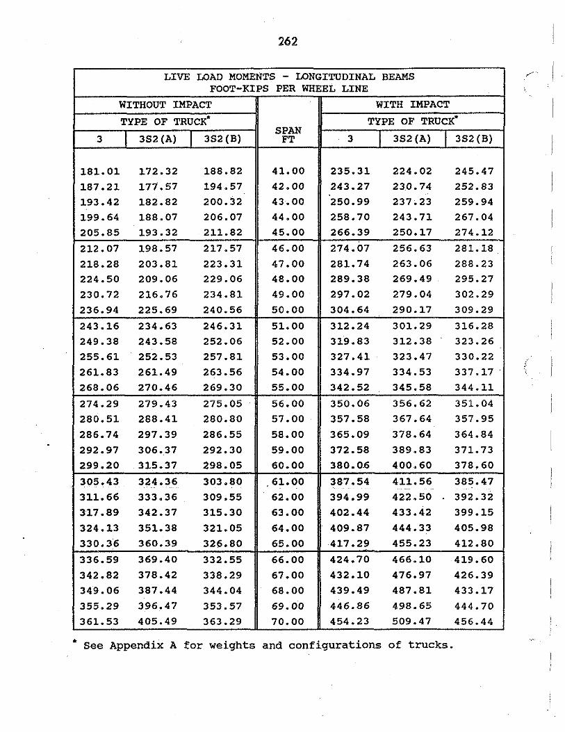
262
LIVE LOAD MOMENTS - LONGITUDINAL BEAMS FOOT-KIPS PER WHEEL LINE
WITHOUT IMPACT . WITH IMPACT
TYPE OF TRUCK* TYPE OF TRUCK*
I I SPAN
I I 3 3S2(A) 3S2(B) FT 3 3S2 (A) 3S2 (B)
181.0l 172.32 188.82 41.00 235.31 224.02 245.47
187.21 177.57 194.57 42.00 243.27 23.0. 74 252.83
193.42 182.82 200.32 43.00 250.99 237.23 259.94
199.64 188.07 206.07 44.00 258.70 243.71 267.04
205.85 193.32 211.82 45.00 266.39 250.17 274.12
212.07 198.57 217.57 46.00 274.07 256.63 281.18
218.28 203.81 223.31 47.00 281.74 263.06 288.23
224.50 209.06 229.06 48.00 289.38 269.49 295.27
230.72 216.76 234.81 49.00 297.02 279.04 302.29
236.94 225.69 240.56 50.00 304.64 290.17 309.29
243.16 234.63 246.31 51.00 312.24 301.29 316.28
249.38 243.58 252.06 52.00 319.83 312.38 323.26
255.61 252.53 257.81 53.00 327.41 323.47 330.22
261.83 261.49 263.56 54.00 334.97 334.53 337.17.
268.06 270.46 269.30 55.00 342.52 345.58 344.ll
274.29 279.43 275.05 56.00 350.06 356.62 351.04
280.51 288.41 280.80 57.00 357.58 367.64 357.95
286.74 297.39 286.55 58.00 365.09 378.64 364.84
292.97 306.37 292.30 59.00 372.58 389.83 371. 73
299.20 315.37 298.05 60.00 380.0.6 400.60 378.60
305.43 324.36 303.80 61.00 387.54 411.56 385.47
311.66 333.36 309.55 62.00 394.99 422.50 . 392.32
317.89 342.37 315.30 63.00 402.44 433.42 399.15
324.13 351.38 321.05 64.00 409.87 444.33 405.98
330. 36 360.39 326.80 65.00 417.29 455.23 412.80
336.59 369.40 332.55 66.00 424.70 466.10 419.60
342.82 378.42 338.29 67.00 432.10 476.97 426.39
349.06 387.44 344.04 ! 68.00 439.49 487.81 433.17
355.29 396.47 353.57 69.00 446.86 498.65 444.70
361.53 405.49 363.29 70.00 454.23 509.47 456.44
* See Appendix A for weights and configurations of trucks.

263
LIVE LOAD MOMENTS - LONGITUDINAL BEAMS FOOT-KIPS PER WHEEL LINE
WITHOUT IMPACT WITH IMPACT
TYPE OF TRUCK* TYPE OF TRUCK*
I I SPAN
I I 3 3S2(A) 3S2 (B) FT 3 3S2 (A) 352 (B)
367.76 414.52 373.01 71.00 461.58 520.27 468.16
374.00 423.56 382.74 72.00 468.92 531.06 479.88 380.24 432.59 392.47 73.00 476.26 541.83 491.58 386.47 441.63 402.22 74.00 483.58 552.59 503.28 392.71 450.67 411.97 75.00 490.89 563.34 514.96
398.95 459.71 421.72 76.00 498.19 574.07 526.63 405.19 468.75 431.49 77.00 505.48 584.78 538.29
411.42 477.90 441.26 78.00 512.76 595.49 549.94 417.66 486.85 451.03 79.00 520.03 606.18 561.58 423.90 495.90 460.81 80.00 527.29 616.85 573 .:n 430.14 504.95 470.60 81.00 534.54 627.51 584.82
436.38 514. 01 480.39 82.00 541. 78 638.16 596.43 442.62 523.06 490.19 83.00 549.02 648.80 608.02 448.86 532.12 499.99 84.00 556.24 659.42 619.60 455.10 541.18 509.79 85.00 563.45 670.03 631.17
461.34 550.24 519.60 86.00 570.66 680.63 642.73 467.58 559.30 529.42 87.00 577.86 691..21 654.28
473.82 568.36 539.24 88.00 585.04 701. 78 665.82 480.06 577.43 549.06 89.00 592.22 712.34 677.35
486.30 586.49 558.89 90.00 599.39 722.89 688.86
492.54 5.95. 56 568.72 91.00 606.56 733.42 700.37 498.78 604.63 578.55 92.00 613.71 743.95 711.86 505.02 613.70 588.39 93 .• 00 620.86 754.46 723.34 511.27 622.77 598.23 94.00 627.99 764.96 734.82 517.51 631. 84 608.08 95.00 635.12 775.44 .746.28
523.75 640.92 617.93 96.00 642.25 795;92 757.73 529.99 649.99 627.78 97.00 649.36 796.39 769.17 536.23 659.07 637.63 98.00 656.47 806.84 780.60 542.48 668.14 647.49 99.00 663.57 817.28 792.02 548.72 677.22 657.35 100.00 670 •. 66 827.71 . 803.43
• See Appendix A for weights and configurations of trucks.

264 LIVE LOAD MOMENTS - LONGITUDINAL BEAMS
FOOT-KIPS PER WHEEL LINE
WITHOUT IMPACT WITH IMPACT .
TYPE OF TRUCK* TYPE OF TRUCK*
I I I HS SPAN
I I I HS 4 3S3 3-3 20 FT 4 3S3 3-3 20
24.50 24.50 22.40 ·40.00 10.00 . 31. 85 31.85 29.12 52.00
29.75 29.75 25.77 44.00 ll.00 38.67 38.67 33.50 57.20
35.00 35.00 29.17 48.00 12.00 45.50 45.50 37.92 62.40
40.25 40.25 32.58 52.00 13.00 52.32 52.32 42.35 67.60
45.50 45.50 36.00 56.00 14.00 59.15 59.15 46.80 72.80
50.75 50.75 39.43 60.00 15.00 65.97 65.97 51.26 78.00
56.00 56.00 42.88 64.00 16.00 72.80 72.80 55.74 83.20
61.25 61.25 46.32 68.00 17.00 79.62 79.62 60.22 88.40
66.50 66.50 49.78 72.00 18.00 86.45 86.45 64.71 93.60
71.75 71.75 53.24 76.00 19.00 93.27 93.27 69.21 98.80
77.00 77.00 56.94 80.00 20.00 100.10 100.10 74.02 104.00
82.25 82.25 62.08 84.00 21.00 106.92 106.92 80.70 109.20
87.50 87.50 67.23 88.00 22.00 113.75 113.75 87.40 114.40
92.75 92.75 72.38 92.00 23.00 120.57 120.57 94.09 119.60
98.00 98.00 77.53 96.00 24.00 127.40· 127.40 100.79 124.80
103.25 103.25 82.69 103.36 25.00 134.22 134.22 107 .• 49 134.37
108.50 108.50 87.86 110.77 26.00 l4:L. 05 141.05 114.20 144.00 113.75 113.75 93.0l 118.22 27.00 147.87 147.87 120.91 153.69
119.00 119.00 98.17 125.71 28.00 154.70 154.70 127.62 163 .• 43
125.39 124.25 103.33 133.24 29.00 163.0l 161.52 134.33 173.21
132.12 129.50 108.50 140.30 30.00 171. 75 168.35 141.05 183.04
138.84 134.75 113.67 148.39 31.00 180.50 175.17 147.77 192.90
145.58 140.00 118.84 156.00 32.00 .189.25 182.00 154.49 202.80
152.32 145.25 124.0l 163.64 33.00 198.0l 188.82 161.21 212.73 159.06 150.50 129.18 171.65 34.00 206.78 195.65 167.93 223.14
165.81 155.75 134.35 180.49 35.00 215.55 202.47 174.65 234.63
172.56 161.00 139.60 189.33 36.00 224.32 209.30 181.49 246.13 179.31 166.25 146.94 198.19 37.00 233.iO 216.12 191.02 257.65 186.07 171.50 155.13 207.05 38.00 241.89 222.95 201.66 269.17
192.83 176.75 163.31 215.92 39.00 250.67 229.77 212.31 280.70
199.59 182.00 171.50 224.80 40.00 259.46 236.60 222.95 292.24
• See Appendix A for weights and configurations of trucks.

265
LIVE LOAD MOMENTS - LONGITUDINAL BEAMS FOOT-KIPS PER WHEEL LINE
WITHOUT IMPACT WITH IMPACT .
TYPE OF TRUCK* TYPE . OF TRUCK*
I I I HS SPAN
I I I HS 4 3S3 3-3 20 FT 4 3S3 3-3 20
206.35 187.25 179.69 233.68 41.00 268.26 243.42 233.59 303.79
213.12 192.50 187.88 242.57 42.00 276.93 250.13 244.12 315.20
219.89 197.75 196.06 251. 4 7. 43.00 285.33 256.60 254.41 326.31
226.66 203.00 204.25 260.36 44.00 293.72 263.06 264.68 337.39
233.43 208.27 212. 44 269.27 45.00 302.09 269.53 274.92 348.46
240.21 215.04 220.63 278.17 46.00 310.44 277.92 285.14 359.51
246.98 221.82 228.81 287.09 47.00 318.78 286.30 295.33 370.54
253.76 229.25 237.00 296.00 48.00 327.10 295.51 305.50 381.55
260.54 237.62 245.19 304.92 49.00 335.41 305.90 315.64 392.54
267.32 246.00 253.38 313.84 50.00 353.70 316.29 325.77 403.51
274.10 254.38 261.56 322.76 51.00 351.97 326.65 335.87 414.46
280.88 262. 77 269.75 331.69 52.00 360.23 337.00 345.95 425.39
287.67 271.16 277.94 340.62 53.00 368.47 347.33 356.01 436.30
294.45 279.56 286.13 349.56 54.00 376.70 357.64 366.05 447.20
301.24 287.95 294.31 358.49 55.00 384.92 367.94 376.07 458.07
308.03 296.36 302.67 367.43 56.00 393.12 378.22 386.28 468.93
314.81 304.76 312.60 376.37 57.00 401.30 3.88. 49 398.48 479.77
321.60 313 .17 322.54 385.31 58.00 409.47 398.74 410.66 490.59
328.39 321.58 332.48 394.25 59.00 417.63 408.97 422.82 501.39
335.18 330.00 342.42 403.20 60.00 425.77 419.19 434.96 512.17
341.97 338.42 352.36 412.15 61.00 433.90 429.39 447.08 522.94
348.77 347.10 362.30 421.10 62.00 442.02 439.90 459.17 533.69
355.56 356.83 372.25 430.05 63.00 450.12 451.73 471.25 544.42
362.35 366.56 382.20 439.00 64.00 458.21 463.54 483.31 555.14
369.15 376.31 392.14 447.95 65.00 466.29 475.34 495.34 565.84
375.94 386.06 402.09 456.91 66.00 474.35 487.12 507.36 576.52 382.73 395.82 412.05 465.87 67.00 482.40 498.90 519.35 587.18
389.53 405.59 422.00 474.82 68.00 490.44 510.66 531.33 597.83
396.33 415. 36 431.95 483.78 69.00 498.47 522.41 543.28 608.47 403.12 425.14 441.91 492.74 70.00 506.49 534.15 555.22 619.09
* See Appendix A for weights and configurations of trucks.

266
LIVE LOAD MOMENTS - LONGITUDINAL BEAMS FOOT-KIPS PER WHEEL LINE
WITHOUT IMPACT WITH IMPACT
TYPE OF TRUCK• TYPE OF TRUCK•
I I I HS SPAN I . 3s3 I I HS 4 3S3 3-3 20 FT 4 3-3 20
409.92 434.93 451.87 501.70 71.00 514.49 545.88 567.14 629.69
416.72 444.72 461.83 510.67 72.00 522.48 557. 60 579 •. ()4 640.28
423.51 454.52 471.79 519.63 73.00 530.46 569.30 590.92 650.85
430.31 464.32 481.75 52.8. 59 74.00 538.43 580.99 602.79 661.41
437.11 474.13 491.71 537.56 75.00 546.39 592.67 614.64 671.95
443.91 483.95 501.67 546.63 76.00 554.33 604.33 626.46 682.48
450. 71 493.77 511.63 555.49 77.00 562.27 615.99 638.28 692.99
457.51 503.59 521.60 564.46 78.00 570.19 627.63 650.07 703.49
464.31 513.42 531.56 573.43 79.00 578.ll 639.26 661.85 713. 98
471.ll 523.25 541.53 582.40 80.00 586.01 650.87 673.61 724.45
477.91 533.09 551.50 591.37 81.00 593.90 662.48 685.36 734.91
484.71 542.93 561.47 600.34 82.00 601.79 674.07 697.09 745.35
491.51 552.77 571.44 609.31 83.00 609.66 685.65 708.80 755.78
498.31 562.62 581.40 618.29 84.00 617.52 697.22 720 •. 50 766.20
505.ll 572.47 591.37 627.26 85.00 625.38 708.77 732.18 776.61
511.91 582.33 601.35 636.23 86.00 633.22 720.02 743.84 787.00
518.71 592.l.8 611.32 645.21 87.00 641.05 731.85 755.50 797.38
525.52 602.05 621.29 654.18 88.00 648.88 743.37 767.13 807.75
532.32 611.91 631. 26 663.16 89.00 656.69 754.88 778.75 818.10
539.12 621.78 641.24 672.13 90.00 664.50 766.38 790.36 828.44
545.93 631.65 651.21 681.11 91.00 672.30 777.86 801.95 838.77
552.73 641.52 661.18 690.09 92.00 680.09 789.34 813.53 849.09
559.53 651.40 671.16 699.06 93.00 687.86 800.80 825.10 859.40
566.34 661.28 681.14 708.04 94.00 695.64 812.25 836.65 869.70
573.14 671.16 691.11 717.02 95.00 703.40 823.69 848.18 879.98
579.94 681.04 701.09 726.00 96.00 711.15 835.12 859.71 890.25
586.75 690.93 711.07 734.98 97.00 718.90 846.54 871.22 900.52
593.55 700.82 721.04 743.96 98.00 726.63 857. 95 882. 71 910.77
600.36 710.71 731.02 752.94 99.00 734.36 869.35 894.20 921.0l
607.16 720.60 741.00 761.92 100.00 742.08 880. 73 905. 67 931.24
* See Appendix A for weights and configurations of trucks.

267
. •I ·~.:.•
APPENDIXC
Questionnaire Document
.· .

269
Iowa Department of Transportation · Highway Division
Research Project HR - 323
Strengthening/Rehabilitation of Low Volume Highway Bridges
Name of Respondent
Organization
Address
The purpose of this questionnaire is to determine your experience and practice in the strengt\lening and/or rehabilitating of. low .. volume highway bridges. For this investigation, bridges with 400 ADT or less are considered low volume. If you wish to comment on any questions or qualify your answers, please use the margins or a separate sheet of paper.
SECTION l
l. Do you (or your county) have any experience with bridge stren,gthening?
Yes __ _ No
with bridge rehabilitation (including replacement)?
Yes __ _ No ---
If yes, please complete Section 2 of this questionnaire.
2. If you answered no to both parts of question l, the reason bridge strengthening and/or rehabilitation has not been used is:
- lack of financial resources
- lack of useful guidelines for decision-making
- lack of trained manpower
- other (please explain)
Note: Check all reasons that are applicable.

270
SECTION 2
l. Recognizing that engineering judgement must be used to make many decisions regarding bridge management, do you typically use more formal methodologies for making management decisions L (e.g. benefit/cost analysis, equivalent annual cost method, etc. I'
Yes No
If yes, which one(s) ?
2. Have you developed any des;gn aids, nomographs, computer software etc., that are useful in making bridge rehabilitation decisions? If so, please describe them.
Yes No
Would you be willing to share them with others?
Yes No
3. Does your county hire a consulting engineer(s) to perform any bridge related structural engineering work?
Yes No
If so, which firm(s) have you employed?

' .
271
4, If a consulting engineer is hired, what type of service is most commonly performed by a consulting engineer?
Structural analysis
construction inspection
Strengthening or rehabilitation
Biannual bridge inspection
other (please describe)?
Check all that apply.
5. Could your county benefit from some sort of decision making tools or design aids for the rehabilitation or strengthening of existing bridges?
Yes __ _ No
What sort of tools would be most helpful to your county?
Computer software
Nomographs
Flow charts
Other (please describe)?
6. If plans or in-house reports are available for any of the strengthening or rehabilitation methods implemented, please indicate who we should contact to obtain copies. ·
Name/Title:
Organization:
Address:

7.
272
With which types of strengthening procedures does your county have experience?
.. .. L s II " .... II .c -c " • • ....
" c L " u Ii ... II • II
" c ... .c
~ -u 0 - E .. ~ D - .. " .. " .. - .... .. " i 0 .c 0. u - -Cl 0 Cl Ol .c .& - b L .. c • ti >-
Cl i - Cl > u .. .. .%: .... .. & - - "' u - > .. Ol .. " "ti .. .. .. - "' c - c "ti 0 c x u - b - "' a.. tl " D 5 .. .. .... a b - c 0 .t:. c 0. - Ii " Cl aJ u Cl Cl .. u -- Cl .t:. L i £ .s-"' " " .... a.. • "ti 0 Ol L .. Ol 0 .. - Cl c 0 I c - l .t:. > L Cl .. " " en 0 u L "ti .. L >
Bridge type <FHWA #) - L c .. "ti 0 .... " ... ...l a. - <n < a. <n Cl Cl
limber stringer (multl beam) (702)
Steel stringer (multi beom) (::102}
Steel pony (380) or thru (J 10) truss
Steel girder & floor beam system (::lOJ
Other (please describe):

273
The following question refers to the structural and cost effectiveness of various strengthening methods. The ratings requested are intended to be a subjective evaluation of the given methods. If a method has met your strengthening objectives, a high rating should be given. Likewise, if a-particular method has been. relatively inexpensive to perform, a high cost effectiveness rating should be given.
a. Based on your experience, please rate the strengthening methods you have employed. Use a scale of 1-10 {10 being the best.)
Strengthening Method Cost Structural Effgctivgngss Effgctivgngss
Lightwaight Oac:l< Raplacamant
Provida compoa1ta action
Incraa.:a tranGvcarGG- 11tiffnC1J1a __
Strangth<1n ax1at1ng mamb11ra
Add or r11ploca mGabara
PoGt-tGnG!on voriova mQolb11ra
Strangth11n crit!col corn11c:tiona .
OavGlop cont1nvlty
Othar Cp!Goaa daacr!ba)1

9.
274
If it is not possible to make an existing bridge structurally adequate to carry legal loads, but it is. possible to strengthen it to carry an increased load, what load would you desire it to carry?
____ Tons
Optionally, rather than specifying a weight Which type of vehicle should the bridge be able to support?
Dump truck ___ _
Dump truck with pup __ _
Farm vehicle __ _
Type of farm vehicle
Other (please describe)
Garbage truck __ _
School bus __ _
10. Do you know of anyone who might be able to supply additional information regarding the rehabilitation and/or strengthening of low volume bridges (e.g. consulting engineers, highway officials, etc.)?
Name:
Organization:
Address:
Name/Title:
organization:
Address:
11. Have you used, or are you familiar with the National Cooperative Highway Research Program Report #293, Methods of Strengthening Existing Highway Bridges?
Yes __ _ No ---
I

275
l2. Previous studies have deterndned that the four bridge types listed below account for over 93% of the structurally deficient bridges on the secondary highway system in Iowa.
Please complete the table below.
Bridge type (FHWA #)
Timber stringer (multi beam) (702) I Steel stringer (multi beam) (302) I Steel pony (380) or thru (310) truss
.
Steel girder & floor beam system (303) I Other (please describe): I
Please return completed questionnaire in the enclosed envelope by June 25. 1990 to:
Dept. of Dr. T. J. Wipf
civil and construction Engineering 420 Town Engineering Iowa State University
Ames, IA 50011


![INDEX [publications.iowa.gov]publications.iowa.gov/28918/1/Iowa_Conservationist_Index_1964_19… · INDEX IOWA CONSERVATIONIST, VOLUMES 23 AND 24 January. 1964, to December. 1965](https://img.pdfslide.us/doc/110x75/5f541c66934bff731c34d6a9/index-index-iowa-conservationist-volumes-23-and-24-january-1964-to-december.jpg)