stichting

mathematisch

centrum

AFDELING MATHEMATISCHE STATISTIEK SW 93/83 (DEPARTMENT OF MATHEMATICAL STATISTICS)

A.J. VAN ES, R.D. GILL & C. VANPUTTEN

RANDOM NUMBER GENERATORS FOR A POCKET CALCULATOR

Preprint

~ MC

JANUARl

kruislaan 413 1098 SJ amsterdam

~Jll.jOH:li:Eli. MATH!ai1r\ TISC:-l c:·>,

~- Au:IST.ERDAM -

Printed at the Mathematical Centre, Kruislaan 413, Amsterdam, The Netherlands.

The Mathematical Centre, founded 11th Februa~v 1946, is a non-profit institution for the promotion of pure and applied mathematics and computer science. It is sponsored by the Netherlands Government through the Netherland, Organization for the Advancement of Pure Research (Z. W.O.).

1980 Mathematics subject classification: Primary 65CI0; Secondary 62 04, 65U05

*) Random number generators for a pocket calculator

by

**) A.J. van Es, R.D. Gill & C. Van Putten

ABSTRACT

Some theory of linear congruential pseudo random number generators

xn+I = (axn+c) mod mis summarized for the case in which the modulus mis

a power of JO. These generators are especially suitable for implementation

on both programmable and non-programmable pocket calculators. Results are

presented of extensive statistical testing of two specific generators.

KEY WORDS & PHRASES: Random nwnber generators, pocket calculators

*) This report will be submitted for publication elsewhere.

**) N.V. Philips gloeilampenfabrieken, Centre for quantitative methods, Eindhoven; formerly at Mathematical Centre, Amsterdam

1. INTRODUCTION

It has recently become practicable to carry out complex statistical

sampling procedures and large simulation experiments using a (programmable)

pocket calculator. This calls for pseudo random number generators which

are quick~ simple and reliable~ especially in the sense that a long stream

of numbers can be safely produced for a single sample or simulation. In

a recent consultation project we came across this need and discovered that,

on the one hand, the ready made generators in the computing literature are

generally aimed at large computers and binary arithmetic (pocket calcula­

tors use decimal arithmetic), while, on the other hand, the random number

generators in manufacturers' statistical packages are sometimes of surpris­

ingly bad quality. In fact one of the recommended generators would produce

a stream of numbers in which a very short subsequence continually repeated

itself if the seed (the first number in the stream) had been chosen unfor­

tunately.

No new theory is presented in this paper. We simply use the standard

theory, to be found in KNUTH (1981), to motivate the choice of two specific

generators from the well-known class of linear congruential generators.

We present the results of extensive statistical testing of the two genera­

tors. The simpler one, which produces 5-figure random numbers, turns out

not to be suitable for widescale use; however the more complicated 9-figure

generator seems to be quite acceptable. We hope that this generator will be

used in practice, or better still, that our paper will stimulate the develop­

ment of better generators, which will also be reported on.

Methods of producing random numbers from distributions other than the

uniform are described by VANPUTTEN & VAN DER TWEEL (1979). Two important

bibliographies are given in SOWEY (1972) and SARAI (1980).

2. LINEAR CONGRUENTIAL GENERATORS WITH MODULUS A POWER OF TEN

Linear congruential generators are defined by the formula

(I) xn+I = (axn + c) mod m

where a,c and mare positive integers, a and c less than m. If a seed

2

x0 is chosen from the set {O,l, .•• ,m-l} then the formula produces a sequen­

ce x 1,x2 , ••• of numbers in the same set, called pseudo random numbers. We

shall only consider generators of the form (I) with m = lOk for some positive

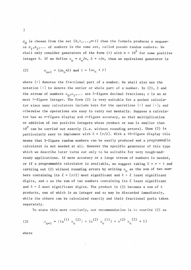
integer k. If we define u = x Im, b = c/m, then an equivalent generator is n n

(2) = {aun + b}

where{•} denotes the fractional part of a number. We shall also use the

notation[•] to denote the entier or whole part of a number. In (2), band

the stream of numbers u0 ,u1, ••• are k-figure decimal fractions; a is an at

most k-figure integer. The form (2) is very suitable for a pocket calcula­

tor since many calculators include keys for the operations{•} and[•]; and

otherwise the operations are easy to car,ry out mentally. Suppose a calcula­

tor has an r-figure display a~d r-figure accuracy, so that multiplication

or addition of two positive integers whose product or sum is smaller than

IOr can be carried out exactly (i.e. without rounding errors). Then (2) is

particularly easy to implement with k = [r/2]. With a IO-figure display this

means that 5-figure random numbers can be easily produced and a programmable

calculator is not needed at all. However the specific generator of this type

which we describe later turns out only to be suitable for very rough-and­

ready applications. If more accuracy or a large stream of numbers is needed,

or if a programmable calculator is available, we suggest taking k = r - I and

carrying out (2) without rounding errors by writing u as the sum of two num-n hers containing its l = [r/2] most significant and k - l least significant

digits, and a as the sum of two numbers containing its l least significant

and k - l most significant digits. The product in (2) becomes a sum of 4

products, one of which is an integer and so may be discarded immediately,

while the others can be calculated exactly and their fractional parts taken

separately.

To state this more concisely, our recommendation is to rewrite (2) as

(3) u = {{a(l) u (2)} + {a( 2) u (l)} + a( 2) u ( 2) + b} n+l n n n

where

4

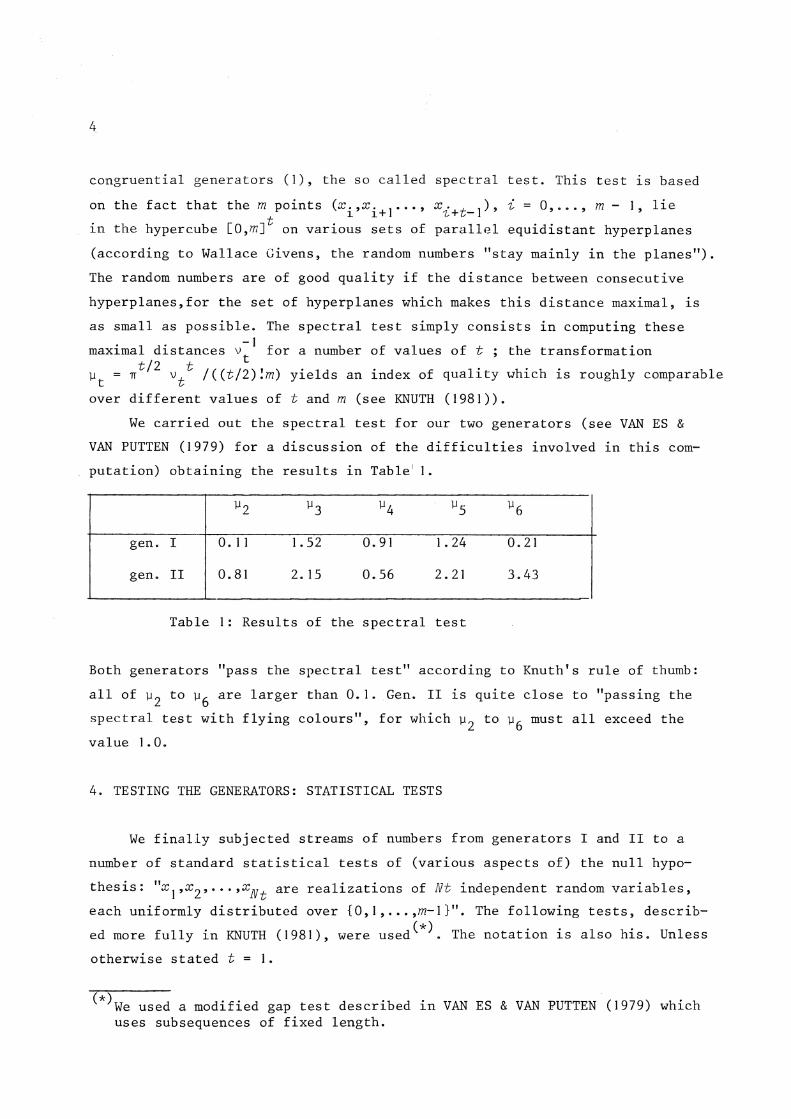
congruential generators (1), the so called spectral test. This test is based

on the fact that the mtpoints (xi,xi+i···• xi+t-l), i = 0, .•• , m - 1, lie

in the hypercube [O,m] on various sets of parallel equidistant hyperplanes

(according to Wallace Givens, the random numbers "stay mainly in the planes").

The random numbers are of good quality if the distance between consecutive

hyperplanes,for the set of hyperplanes which makes this distance maximal, is

as small as possible. The spectral test simply consists in computing these

maximal distances v~ 1 for a number of values oft; the transformation t/2 t . µt = TT vt /((t/2)!m) yields an index of quality Yhich is roughly comparable

over different values oft and m (see KNUTH (1981)).

We carried out the spectral test for our two generators (see VAN ES &

VANPUTTEN (1979) for a discussion of the difficulties involved in this com­

putation) obtaining the results in Table' 1.

µ2 µ3 µ4 µ5 µ6

gen. I 0. 1 1 1. 52 0.91 1. 24 0.21

gen. II 0.81 2. 15 0.56 2.21 3.43

Table I: Results of the spectral test

Both generators "pass the spectral test" according to Knuth's rule of thumb:

all of µ2 to µ6 are larger than 0. 1. Gen. II is quite close to "passing the

spectral test with flying colours", for which µ2 to µ6 must all exceed the

value 1. O.

4. TESTING THE GENERATORS: STATISTICAL TESTS

We finally subjected streams of numbers from generators I and II to a

number of standard statistical tests of (various aspects of) the null hypo­

thesis: "x 1,x2 , ... ,xNt are realizations of Nt independent random variables,

each uniformly distributed over {O,l, ..• ,m-1}". The following tests, describ­

ed more fully in KNUTH (1981), were used(*). The notation is also his. Unless

otherwise stated t = 1.

(*)we used a modified gap test described in VAN ES & VANPUTTEN (1979) which uses subsequences of fixed length.

d. f. N (i) Kolmogorov-Smirnov test 100

(ii) Frequency test (d=5 I , t=2) 50 1000

(iii) Serial test (d=I0) 99 1000

(iv) Gap test (a=0,B= I t = 7) 7 1000 2'

(v) Gap test (a=¼, B= 3 t 7) 7 1000 4 ,

(vi) Gap test (a=½, B= 1 ' t = 7) 7 1000

(vii) Partition test (d=5, t = 4) 3 1000

(viii) Coupon Collector's test (d=5, t= I 0) 5 500

(ix) Permutation test (t=4) 23 1000

(x) Run test (up) 6 5000

(xi) Run test (down) 6 5000

All but the first test (Kolmogorov-Smirnov) yield statistics which,

under the null hypothesis, are approximately x2-distributed for large N.

The column "d.f." contains the corresponding number of degrees of freedom.

Each test was carried out 40 times for each generator, except that we did

not carry out the run tests for gen. I since these tests use more than the . (*)

whole cycle for this generator . For gen. II, except for the Kolmogorov-

Smirnov test, all tests were carried out on disjunct subsequences of

.)

length Nt of the sequence{x0 ,x 1, •.. ,xm-l}. These test results are therefore,

under the null hypothesis, independent, and may be combined in various ways.

We have combined the results for gen. II in the following ways:

(i) For each test we have counted the number of significant values at

the a= .05 level.

(ii) Apart from test (i), for each test we have computed the sum of the

40 realizations which,under the null hypothesis, is also a realization

of an approximately x2-distributed random variable.

(iii) We have computed the Fisher combination of the 40 p-values (right

tail probabilities) for each test (comparing -2L~O log p. with the 1,= I 1,

x2-distribution with 80 degrees of freedom).

(iv) A Fisher combined test has also been carried out for all J0x40 p­

values for tests (ii) to (xi).

(*)Admittedly this also applies to tests (iv) to (ix).

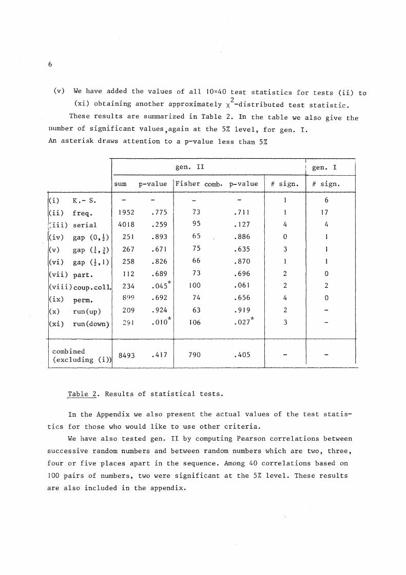
6

(v) We have added the values of all I0x40 test statistics for tests (ii) to

(xi) obtaining another approximately x2-distributed test statistic.

These results are summarized in Table 2. In the table we also give the

number of significant values,again at the 5% level, for gen. I.

An asterisk draws attention to a p-value less than 5%

I gen. II i gen. I

sum p-value Fisher comb. p-value # sign. # sign.

(i) K. - S. - - - - I 6

(ii) freq. 1952 . 775 73 . 7 1 1 1 17

:<iii) serial 4018 .259 95 . 12 7 4 4 ,,

(iv) gap (0, ½) 251 .893 65 i .886 0 I

(v) gap CLV 267 . 671 75 .635 3 1

(vi) gap (½,I) 258 .826 66 .870 1 1

(vii) part. I 12 .689 73 . 696 2 0

(viii) coup. coll. 234 .045 * 100 .061 2 2

(ix) perm. 89Q .692 74 .656 4 0

(x) run(up) 209 .924 63 .919 2 -(xi) run(down) 291 . 010 * 106 .027 * 3 -

combined 8493 .417 790 .405 - -(excluding (i))

Table 2. Results of statistical tests.

In the Appendix we also present the actual values of the test statis­

tics for those who would like to use other criteria.

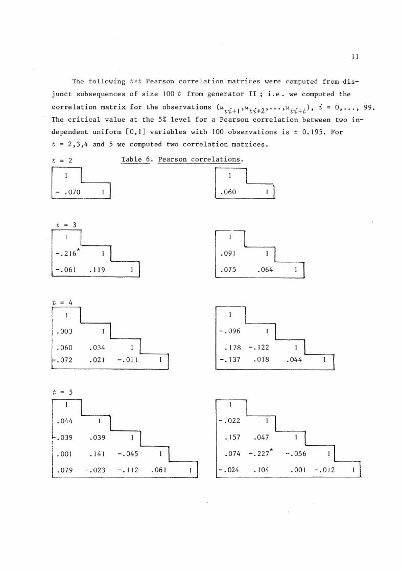
We have also tested gen. II by computing Pearson correlations between

successive random numbers and between random numbers which are two, three,

four or five places apart in the sequence. Among 40 correlations based on

100 pairs of numbers, two were significant at the 5% level. These results

are also included in the appendix.

7

5. CONCLUSIONS

Generator I. This generator is unfortunately of rather poor quality.

Both the Kolmogorov-Smirnov test and the frequency test give bad results;

these two tests are tests of uniformity over {0,1, .•. ,m-I} which is perhaps

the most crucial requirement for a pseudo random number generator.

Generator II. In general the results for this generator are very satisfac­

tory. Especially the behaviour under Kolmogorov-Smirnov and frequency tests

is excellent. The only test which suggests a bad aspect of the generator

is the run test (down).

Advice for use. If at all possible use gen. II. In general, when using either

generator, we suggest the following rule of thumb: if an application needs N

pseudo random numbers, then do not rely on the last log10 N + 2 digits of

the decimal fractions u 1 ,u2 , ... ,uN.

The reason for this advice is that the last figures of the numbers from

a generator (I) show very clear systematic behaviour (the last figure follows

a cycle of length IO, etc.). The more numbers are required, the more serious

this is.

REFERENCES

VAN ES, A.J. & C. VANPUTTEN (1979), The Statal random number generator,

report SN 8/79, Mathematical Centre, Amsterdam.

KNUTH, D.E. (1981), The art of computer programming, Vol. II, Seminumerical

algorithms (2nd edition), Addison-Wesley, Reading, Massachusetts.

VAN PUTTEN, C. & I. VAN DER TWEEL ( I 979), On generating random variables,

report SN 9/79, Mathematical Centre, Amsterdam.

SARAI, H. (1980), A supplement to Sowey's bibliography on random number

generation and related topics, Biom. J. 22 447-461.

SOWEY, E.R. (1972), A chronological and classified bibliography on random

number generation and testing, Int. ,Stat. Rev. 40 355-371.

8

APPENDIX

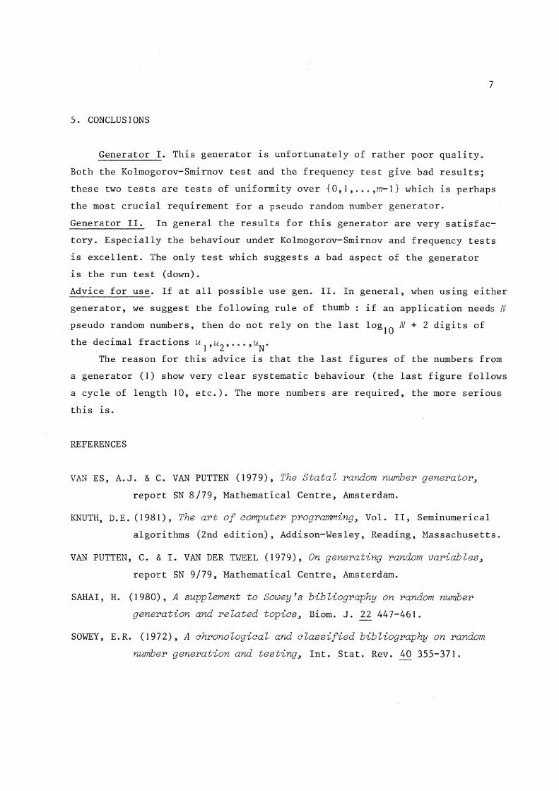
Table 3. Results of Kolmogorov-Smirnov test (* denotes significance at 5%

level)

gen. I ~en. II

value of p-value value of p-value test statistic test statistic

0.058 0.881 0.075 0.986

o. 112 0.160 0.120 0.108

0.060 0.857 0.111 0.163

0.094 0.338 0.090 0.391

0.088 0.416 0.090 0.380

* 0.153 0.017 0.061 0.840

* 0.166 0.007 0.043 0.991

0.059 0.874 0.068 0. 728

o. 128 0.074 0.107 0.194

o. IOI 0.258 0.064 0.802

0.069 0.719 0.083 0.485

0.056 0.912 0.067 0.752

* 0.143 0.032 0.086 0.448

0.059 0.873 * 0.136 0.048

0.072 0.674 0.054 0.927

(}. I 07 0.201 0.103 0.235

0.061 0.848 0.056 0.443

0.103 0.230 0.128 0.072

* 0.161 0.010 0.090 0.391

0.091 0.365 0.091 0.373

0.046 0.980 0.056 0.906

0.064 0.803 0.103 0.230

0.074 0.638 0.065 0.788

0.073 0.652 0.063 0.819

0.110 0.175 0.111 0.166

0.073 0.649 0.098 0.285

0.107 0.200 0.090 0.382

0.075 0.618 0.062 0.828

0.089 0.404 0.073 0.650

0.073 0.655 0.065 o. 785

* 0.138 0.042 0.076 0.601

* o. 161 0.010 0.073 0.656

0.050 0.961 0.056 0.902

0.133 0.057 0.118 0.120

0.106 0.210 0.116 0.120

0.054 0.927 0.096 0.396

0.051 0.957 0.135 0.051

0. I 18 0.119 0.076 0.604

0.074 0.634 0.122 0.099

0.087 0.432 0.064 o. 796

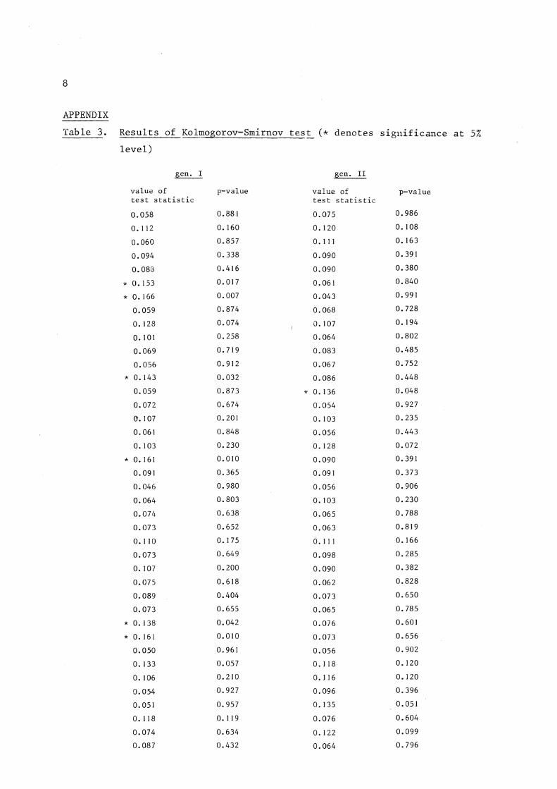
9 Table 4.

Results of statistical tests (ii)-(ix) for generator I(* denotes significance

at 5% level; note subcycles in columns (iii) and (vii))

(ii) (iii) (iv) (v) (vi) (vii) (viii) (ix)

* 68.4 90.6 8.90 4. 32 4.92 0.67 8.30 16.7

* 78.0 92.4 5.21 6.09 6.40 I. 51 6.82 21. I

64.6 86.0 8.01 7. 07 11.53 0.44 7. 9 I 22.9

5 I. 0 *132.2 4. 77 *26.98 12.31 4.85 7.75 27.4

62.0 94.4 9. 9 I 8.63 2.75 0.32 4.84 17.5

43.7 99.4 3.35 I. 87 3.55 0.67 *13.68 19.5

* 77 .5 I 14.0 7.48 4.56 7.48 l. 51 7. 29 14.6

66.9 70.0 10.23 11. 54 8.08 0.44 7.37 23.5

54.3 98.0 5.89 5.88 8.95 4.85 10.94 29.6

61. 3 97.0 7.91 8.95 2.06 0.32 10.85 21. 0

* 68.4 90.6 5.34 3.51 2.27 0.67 6. 15 17.8

* 78. I 92.4 I. 79 10.88 8.24 I. 51 3.61 18.3

* 75.3 86.0 8.36 10. 85 2.62 0.44 4.33 34.8

53.7 *132.2 8. 18 7.52 *14.79 4.85 6. I 7 18.8

* 76.0 94.4 IO. 31 6.50 6. I 3 0.32 8.87 19.5

64.9 99.4 2.65 6.27 11.06 0.67 8.43 17.3

* 68. I 114. 0 4.50 12. 71 6.69 1.51 6.28 I 7. 5

67. I 70.0 10.65 12.83 5.00 0.44 3.53 18.2

59. I 98.0 7.26 3.09 5.08 4.85 4.83 14. 9

57.2 97.0 6.53 6.71 4. 31 0.32 4.83 23. I

43.4 90.6 8.55 9.95 10.94 0.67 8.30 17.4

* 79. I 92.4 7. I 7 1.49 11.80 1.51 6.82 23.3

* 70.4 86.0 I. 95 8.39 4.96 0.44 7.91 27.2

50.5 *132.2 11.80 5.81 3.53 4.85 7.75 23.0

66.7 94.4 5.88 0. 7 I 8.37 0.32 4.48 15.8

* 75. I 99.4 I. 54 6.29 3.73 0.67 *13.68 11.0

* 79.6 I 14.0 9.78 2.24 8.06 I. 51 7. 29 16.5

* 74.2 70.0 2. 96 2.53 6.76 0.44 7.37 21. 4

56.4 98.0 10.40 4.82 8.90 4.85 10.94 22.2

* 7 I. 4 97.0 6.25 9.37 5.21 0.32 10.85 22.4

65.0 90.6 2.69 21. 99 8.01 0.67 6. 15 21. 5

66.8 92.4 7.67 6.38 4. 77 I. 51 3.61 23.4

62.9 86.0 4.34 6.01 9.91 0.44 4.33 18. 2

62.2 *132.2 8.06 11. 57 3.35 4.85 6. I 7 14.6

55.3 94.4 5.98 4.26 7.48 0.32 8.87 14.2

43. I 99.4 I. 22 8.07 10.23 0.67 8.43 I 9.0

* 74.7 I 14.0 4.32 4.92 5.89 1.51 6.28 18.5

* 69.6 70.0 6.09 6.40 7. 91 0.44 3.53 20.3

47.7 98.0 7.07 I I. 53 5.34 4.85 4.82 26.5

* 70.5 97.0 *26.98 I 2. 31 I. 79 0.32 4.83 23.9

IO

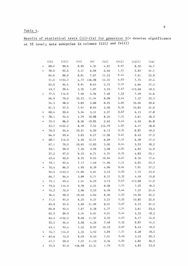
Table 5.

Results of statistical tests (ii)-(xi) for generator II.(* denotes signiffcance

at 5% level)

(ii) (iii) (iv) (v) (vi) (vii) viii) (ix) (x) (xi)

57.4 100.6 9.56 6.62 4.20 2.03 8.24 32.8 3.92 5.47

46.3 111. 4 10.86 0.82 *18.27 5.55 9.53 27.7 2.43 4.50

39.3 99.4 3. 31 7.76 10.95 1.20 6.39 28.6 5.32 7.33

52.5 91. 2 3.52 7. 96 7.58 2.87 2.55 15.8 1.87 9.26

58.1 77.8 7.75 3.52 4.52 1.86 7.66 16.5 *16.35 *15.24

48.7 83.4 4.09 10.53 0.99 3.53 4.32 18.3 6.18 6.98

47.7 *125.8 10.00 6.81 5. 72 0.93 5.89 26.4 8.33 8.99

62.2 76.0 8.91 4.69 7 .92 6.85 7.98 18.2 *I .OS *17 .19

45.1 86.4 8.01 1.80 8.37 0.69 4.26 *38.9 I. 40 5.59

40.2 81 .o 10.60 3.57 5.76 3.22 2. 14 15.5 7.22 5.69

47.3 83.8 12.99 5.10 4.13 3.34 3.76 22. I 4.76 6.10

48.7 95.6 6.38 7 .14 7.57 *8.88 6.22 27.8 9.17 6.21

44.4 *136.2 0.56 7. 10 7.43 1. 193 9.34 11. 7 2.03 8. 72

43.3 96.2 7.07 6.87 1.86 I. 29 7.39 21.5 4.08 3.32

42.4 97.4 10.49 7.68 4. 15 0.79 7.00 19.2 3.30 10.16

52.7 92.4 5.57 *14.37 7.75 3.84 4.84 19.5 2.44 6.42

43.2 84.0 5.00 5.60 5.31 2. 14 9.55 26.0 7.01 6.57

34.5 90.4 11.87 6.37 3.84 1.37 3.91 23. I 3.23 s. 77

46.4 87.6 5.87 7.62 7.71 0.76 4.09 18.7 2. 77 8.35

51.7 107.0 0.53 6.65 3.94 2. 16 3.59 15.2 7.94 11. 27

*85.0 122.6 6. 19 8.49 4.62 4.57 2.94 19.3 2.66 I. 99

38.8 96.2 5.96 4.07 7.01 4.11 2. 19 20.6 6.70 9.68

56.4 *143.8 5.24 4.73 4.65 0.37 4.04 13.2 7.36 3.64

44.6 112.4 6.32 3.41 4.69 0.51 *12.04 22.3 3.16 2.46

23.7 88.4 3.23 9.50 6.52 5.18 9.66 18.4 4.42 5.77

38.6 110.6 8.85 2.42 4.86 I. 22 2.56 22.3 4.34 3.32

50.3 98.8 I. 75 *21.56 s. 72 2.44 7.50 19.8 8.63 4.24

52.2 114.8 4.31 13.22 9.37 5.27 1.80 *35.9 1.40 11.52

27.6 120.6 1.35 4.04 8.81 1.42 1.07 16. 1 7.00 *15.73

46.1 84.2 1.94 4.84 11.29 1.01 1.20 13.9 4.87 10.38

41.9 98.4 9.80 4. 75 10.86 1.80 3.99 *36.4 5.62 3.98

58.4 116.0 4.76 5.41 5.12 3.02 2.94 27.0 8.39 5.26

56.0 110.4 5.61 5.34 4.14 3.00 3.36 26.8 5.85 6.42

49.5 83.6 9.44 10.12 3.80 1.82 4.86 *37.2 5.29 6.69

53.6 101.4 9.97 5.17 5.00 0.91 5.87 16.8 12.72 6.55

64.1 86.8 5.23 2.08 4.70 4.91 *20.04 21. 6 3.07 3.88

53.5 93.0 3.66 5.92 10.65 1.32 5.36 23.7 3.86 12.28

46.8 104.2 4.67 5.20 8.64 *8.38 6.68 24.6 6.56 6.07

62.4 *130.0 4.13 *14.35 4.28 4.66 9.92 18.2 2.58 6.08

so.a 98.0 5.25 6.35 4.90 0.95 7.26 21.0 3.36 6.36

I I

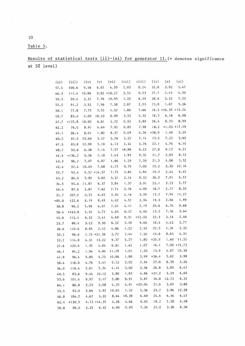
The following txt Pearson correlation matrices were computed from dis­

junct subsequences of size 100 t from generator II; i.e. we computed the

correlation matrix for the observations (uti+l'uti+2 , ... ,uti+t)' i = 0, ... , 99.

The critical value at the 5% level for a Pearson correlation between two in­

dependent uniform [0,1] variables with 100 observations is± 0.195. For

t 2,3,4 and 5 we computed two correlation matrices.

t = 2

- .070

t = 3

J1] __ -.216

-.061

t = 4

.003

.060

.072

t = 5

.044

~.039

.001

.079

• I I 9

.034

.021

.039

. 1 4 1

-.023

Table 6. Pearson correlations.

.060

.091

.075

- . 096

.064

.178 -.122

- . 01 1 - . 137 .018

- . 022

. 157 .047

-.045 .074 -.227 *

- . 1 12 .061 - . 024 • I 04

.044

-- . 056

.001 -.012