S th i f i f ll ti i i hi h t l l ti t i hSynthesis of rainfall timeseries in a high temporal resolution – a parametric approachSynthesis of rainfall timeseries in a high temporal resolution – a parametric approachy g p p ppAna Claudia Callau Poduje & Uwe HaberlandtAna Claudia Callau Poduje & Uwe Haberlandt

d Parameters regionalization1 Motivation & Objectives 3 Study Area & Data Parameters regionalization1. Motivation & Objectives 3. Study Area & Data g. ot at o & Object es y

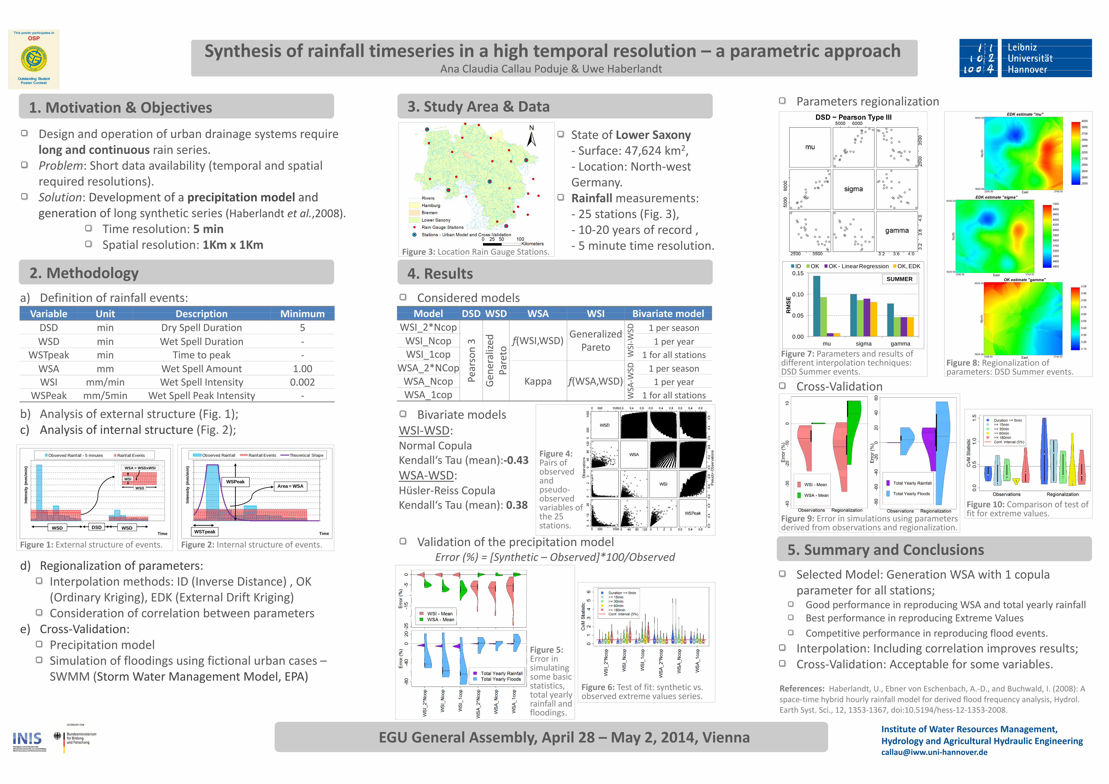
D i d ti f b d i t i S f L SDesign and operation of urban drainage systems require State of Lower SaxonyDesign and operation of urban drainage systems require  State of Lower Saxonylong and continuous rain series Surface: 47 624 km2long and continuous rain series. ‐ Surface: 47,624 km2,g

bl Sh d il bili ( l d i l, ,

Problem: Short data availability (temporal and spatial ‐ Location: North‐westProblem: Short data availability (temporal and spatial  ‐ Location: North‐west required resolutions) Grequired resolutions). Germany.required resolutions). Germany.Solution: Development of a precipitation model and Rainfallmeasurements:Solution: Development of a precipitation model and  Rainfall measurements:p p p

ti f l th ti i (H b l d l 2008) 2 i ( i 3)generation of long synthetic series (Haberlandt et al 2008) ‐ 25 stations (Fig 3)generation of long synthetic series (Haberlandt et al.,2008). 25 stations (Fig. 3),Time resolution: 5 min 10 20 years of recordTime resolution: 5 min ‐ 10‐20 years of record ,

l l0 0 years of record ,

Spatial resolution: 1Km x 1Km ‐ 5 minute time resolutionSpatial resolution: 1Km x 1Km ‐ 5 minute time resolution.Figure 3: Location Rain Gauge StationsFigure 3: Location Rain Gauge Stations.ID OK OK Li R i OK EDK2 Methodolog 4 R ltID OK OK - Linear Regression OK, EDK2. Methodology 4. Results 0.152. Methodology 4. Results SUMMER

C id d d l) D fi iti f i f ll t 0 10Considered modelsa) Definition of rainfall events: 0.10

EConsidered modelsa) Definition of rainfall events:

MS

Model DSD WSD WSA WSI Bivariate modelVariable Unit Description Minimum RM

Model DSD WSD WSA WSI Bivariate modelVariable Unit Description Minimum 0.05

R

WSI 2*N D 1p

DSD i D S ll D ti 5 WSI 2*Ncop G li d SD 1 per seasonDSD min Dry Spell Duration 5 _ p

d  f( ) Generalized WS 1 per seasonDSD min Dry Spell Duration 5

0 003 ed f(WSI,WSD) Generalized 

‐WWSI Ncop 1 per yearWSD min Wet Spell Duration ‐ 0.00mu sigma gamma

n 3 ze o

f(WSI,WSD) Pareto SI‐WSI_Ncop 1 per yearWSD min Wet Spell Duration mu sigma gamma

on li to Pareto

WS

WSI 1cop 1 for all stationsWSTpeak min Time to peak Figure 7: Parameters and results ofso ra ret WWSI_1cop 1 for all stationsWSTpeak min Time to peak ‐

Fi re 8 R i li ti fFigure 7: Parameters and results of different interpolation techniq esar

s er arWSA 2*NCop D 1 per seasonWSA mm Wet Spell Amount 1 00 Figure 8: Regionalization of different interpolation techniques: 

ea ne PaWSA_2*NCop

WS 1 per seasonWSA mm Wet Spell Amount 1.00 g g

parameters: DSD Summer eventsp q

DSD Summer events

Pe en P

K f(WSAWSD) W

pWSA N 1

pWSI / i W t S ll I t it 0 002

parameters: DSD Summer events.DSD Summer events.

Cross ValidationP Ge Kappa f(WSA,WSD) A‐WWSA Ncop 1 per yearWSI mm/min Wet Spell Intensity 0.002 Cross‐ValidationG pp f( , )

SA

_ p p yWSA 1

WSI mm/min Wet Spell Intensity 0.002/ WWSA 1cop 1 for all stationsWSPeak mm/5min Wet Spell Peak Intensity ‐ WWSA_1cop 1 for all stationsWSPeak mm/5min Wet Spell Peak Intensity

b) A l i f l (Fi 1) Bivariate modelsb) Analysis of external structure (Fig 1); Bivariate modelsb) Analysis of external structure (Fig. 1);WSI WSDc) Analysis of internal structure (Fig 2) WSI‐WSD:c) Analysis of internal structure (Fig. 2); WSI WSD:c) Analysis of internal structure (Fig. );Normal CopulaNormal Copula

Fi re 4K d ll‘ T ( ) 0 43Observed Rainfall - 5 minutes Rainfall Events 1 5 9 13 17 21 25 29 33 37 41 45 49 53 57 61 65 69 73 77 81 85 89 93 97 101

Observed Rainfall Rainfall Events Theoretical Shape Figure 4: Kendall‘s Tau (mean):‐0.435 9

0.20.20g

Pairs of( )

n) WSA = WSDxWSI 0.180.18n)

Pairs of observedWSA‐WSD:/m

i

0.160.16/mi observed WSA‐WSD:

mm

/

WSI 0.140.14

mm

/

WSPeakWSPeak andHü l R i C ly

(m

WSD0.120.12y

(m WSPeakWSPeakArea = WSA

and pseudoHüsler‐Reiss Copula ns

ity WSD0.10.10

nsity pseudo‐p

d ll‘ ( )nten 0.080.08

nten observedKendall‘s Tau (mean): 0 38In 0.060.06In

observed variables of Figure 10: Comparison of test ofKendall s Tau (mean): 0.380.040.04 variables of  Figure 10: Comparison of test of 

fit for extreme values0.020.02 the 25 Figure 9: Error in simulations using parameters fit for extreme values.00.00

the 25 stations

Figure 9: Error in simulations using parameters d i d f b i d i li iWSD DSD WSD

WSTpeakWSTpeakstations. derived from observations and regionalization.

Time TimeWSTpeakWSTpeak g

Validation of the precipitation modelFi 1 E t l t t f t Fi 2 I t l t t f t Validation of the precipitation model  5 Summary and ConclusionsFigure 1: External structure of events. Figure 2: Internal structure of events.E (%) [S th ti Ob d]*100/Ob d 5. Summary and Conclusionsg gError (%) = [Synthetic – Observed]*100/Observed y

d) l f( ) [ y ] /

d) Regionalization of parameters:Selected Model: Generation WSA with 1 copula

d) Regionalization of parameters:Selected Model: Generation WSA with 1 copula I t l ti th d ID (I Di t ) OK pInterpolation methods: ID (Inverse Distance) , OKparameter for all stations;

Interpolation methods: ID (Inverse Distance) , OK parameter for all stations;(Ordinary Kriging) EDK (External Drift Kriging) Good performance in reproducing WSA and total yearly rainfall(Ordinary Kriging), EDK (External Drift Kriging) Good performance in reproducing WSA and total yearly rainfall( y g g) ( g g)

C id ti f l ti b t tp p g y y

B t f i d i E t V lConsideration of correlation between parameters Best performance in reproducing Extreme ValuesConsideration of correlation between parameters p p ge) Cross Validation: Competitive performance in reproducing flood eventse) Cross‐Validation: Competitive performance in reproducing flood events.)

I t l ti I l di l ti i ltPrecipitation model Interpolation: Including correlation improves results;Precipitation model Figure 5: Interpolation: Including correlation improves results;Si l ti f fl di i fi ti l b

Figure 5: Error in Cross Validation: Acceptable for some variablesSimulation of floodings using fictional urban cases – Error in  Cross‐Validation: Acceptable for some variables.Simulation of floodings using fictional urban cases simulating p

SWMM (Storm Water Management Model EPA)simulating some basicSWMM (Storm Water Management Model, EPA) some basic 

References: Haberlandt U Ebner von Eschenbach A D and Buchwald I (2008): A( g , )

statistics, Figure 6: Test of fit: synthetic vs References:  Haberlandt, U., Ebner von Eschenbach, A.‐D., and Buchwald, I. (2008): A statistics, total yearly

Figure 6: Test of fit: synthetic vs. b d t l i space‐time hybrid hourly rainfall model for derived flood frequency analysis Hydroltotal yearly 

i f ll dobserved extreme values series. space time hybrid hourly rainfall model for derived flood frequency analysis, Hydrol. 

/rainfall and 

Earth Syst. Sci., 12, 1353‐1367, doi:10.5194/hess‐12‐1353‐2008.rainfall andfloodings Earth Syst. Sci., 12, 1353 1367, doi:10.5194/hess 12 1353 2008.floodings.

Institute of Water Resources ManagementEGU General Assembly April 28 May 2 2014 Vienna Institute of Water Resources Management, EGU General Assembly, April 28 – May 2, 2014, Vienna Hydrology and Agricultural Hydraulic Engineeringy, p y , , Hydrology and Agricultural Hydraulic Engineeringcallau@iww.uni‐hannover.deca au@ .u a o e .de