Stereo vision- facing the challenges and seeing the

Stereo vision— Facing the challenges and seeing the opportunities for ADAS applications

Aish DubeyADAS

Texas Instruments

Stereo vision—Facing the challenges and seeing 2 July 2020the opportunities for ADAS applications

Introduction

Cameras are the most precise mechanisms used to capture accurate data at high resolution. Like human eyes, cameras capture the resolution, minutiae and vividness of a scene with such beautiful detail that no other sensors such as radar, ultrasonic and lasers can match. The prehistoric paintings discovered and dated back tens of thousands of years ago in caves across the world are testaments that pictures and paintings coupled with visual sense have been the preferred method to convey accurate information [1].

The next engineering frontier, that some might argue will be the most challenging for the technology community, is real-time machine vision and intelligence. The applications include, but are not limited to, real-time medical analytics (surgical robots), industrial machines and cars that are driven with autonomous intelligence. In this particular paper, we will focus on autonomous Advanced Driver Assistance Systems (ADAS) applications and how cameras and stereo vision in particular is the keystone for safe, autonomous cars that can “see and drive” themselves.

The key applications that require cameras for ADAS are shown below in Figure 1. Some of the applications shown can be implemented using just a vision system such as forward-, rear- and side-mounted cameras for pedestrian detection, traffic sign recognition, blind spots and lane detect systems. Others such as intelligent adaptive cruise control can be implemented robustly as a fusion of radar data with the camera sensors, especially for complex scenarios such as city traffic, curvy non-straight roads or higher speeds.

Figure 1: Applications of camera sensors for ADAS in a modern vehicle: (a) Forward facing camera for – lane detect, pedestrian detect, traffic sign recognition and emergency braking. (b) Side- and rear-facing cameras for parking assistance, blind spot detection and cross traffic alerts


What kind of camera is needed?

All the real world scenes that a camera encounters

are three dimensional. The objects that are at

different depths in real world may appear to be

adjacent to each other in the two-dimensional

mapped world of the camera sensor. Figure 2

shows a picture from the Middlebury image

dataset [2]. Clearly the motor bike in the foreground

of the picture is about two meters closer to the

camera than the storage shelf in the background.

Please pay attention to point 1 and 2 annotated

in the figure. The red box (point 1) that is in the

background appears adjacent to the forks (2) of the

bike in the captured image, even though it is at least

two meters farther away from the camera. Human

brain has the power of perspective that allows us to

make the decision about depth from a 2-D scene.

For a forward-mounted camera in the car, the ability

to analyze perspective does not come as easy.

If we have a single camera sensor mounted and

capturing video that needs to be processed and

analyzed, that system is called a monocular (single-

eyed) system, whereas a system with two cameras,

separated from each other is called a stereo vision

system. Before we go any further, please have a

look at Table 1 that compares the basic attributes

of a monocular-camera ADAS with a stereo-camera

system.

Comparison parameter

Mono-camera system

Stereo-camera system

Number of image sensors, lenses and assembly

1 2

Physical size of the system

Small (6” × 4” × 1”) Two small assemblies separated by

~25–30 cm distance

Frame rate 30 to 60 frames per second

30 frames per second

Image processing requirements

Medium High

Reliability of detecting obstacles and emergency braking decisions

Medium High

System is reliable for Object detection (lanes, pedestrians, traffic

signs)

Object detection “AND”calculate distance-to-

object

System cost 1× 1.5×

Software and algorithm complexity

High Medium

Table 1: High-level comparison of system attributes for a mono- vs. stereo-camera ADAS system

The monocular-camera-based video system can

do many things reasonably well. The system and

analytics behind it can identify lanes, pedestrians,

many traffic signs and other vehicles in the path of

the car with good accuracy. Where the monocular

system is not as robust and reliable is in calculating

the 3-D view of the world from the planar 2-D frame

that it receives from the single camera sensor. That’s

not surprising if we consider the natural fact that

humans (and most advanced) animals are born with

Figure 2: Image from 2014 Middlebury database. The motor bike in the foreground is much closer to the camera than the storage shelf, though all objects appear adjacent in a 2-D mapped view.

Point 2 – forks of motor bike

Point 1 – red box on shelf


two eyes. Before analyzing this problem in further

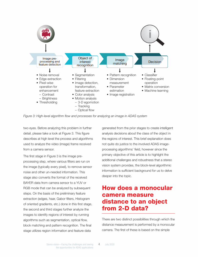
detail, please take a look at Figure 3. This figure

describes at high level the process and algorithms

used to analyze the video (image) frame received

from a camera sensor.

The first stage in Figure 3 is the image pre-

processing step, where various filters are run on

the image (typically every pixel), to remove sensor

noise and other un-needed information. This

stage also converts the format of the received

BAYER data from camera sensor to a YUV or

RGB mode that can be analyzed by subsequent

steps. On the basis of the preliminary feature

extraction (edges, haar, Gabor filters, Histogram

of oriented gradients, etc.) done in this first stage,

the second and third stages further analyze the

images to identify regions of interest by running

algorithms such as segmentation, optical flow,

block matching and pattern recognition. The final

stage utilizes region information and feature data

generated from the prior stages to create intelligent

analysis decisions about the class of the object in

the regions of interest. This brief explanation does

not quite do justice to the involved ADAS image-

processing algorithms’ field, however since the

primary objective of this article is to highlight the

additional challenges and robustness that a stereo

vision system provides, the block-level algorithmic

information is sufficient background for us to delve

deeper into the topic.

How does a monocular camera measure distance to an object from 2-D data?

There are two distinct possibilities through which the

distance measurement is performed by a monocular

camera. The first of these is based on the simple

Figure 3: High-level algorithm flow and processes for analyzing an image in ADAS system

• Noise removal• Edge extraction• Pixel-wise

operation forenhancement– Contrast– Brightness

• Thresholding

• Segmentation• Filtering• Image detection,

transformation,feature extraction

• Color analysis• Motion analysis

– 3-D egomotion– Tracking– Optical flow

• Pattern recognition• Dimension

measurement• Parameter

estimation• Image registration

• Classifier• Floating-point

operation• Matrix conversion• Machine learning


premise that the objects closer to the camera

appears bigger, and therefore takes up a larger pixel

area in the frame. If an object is identified as a car,

then the size of the object can be approximated by

a maximum-covering-rectangle drawn around it.

The bigger the size of this rectangle, the closer that

object is to the camera (i.e. the car). The emergency

braking algorithm will assess if the distance to each

object identified in the frame is closer than a safe

predefined value, then initiate the collision avoidance

or driver warning actions as necessary. See Figure 4

for a simple illustration of this idea.

Simplicity and elegance are both benefits of this

method, however there are some drawbacks to

this approach. The distance to any identified object

cannot be assessed until the object is pre-identified

“correctly”. Consider the scenario shown in Figure

5. There are three graphical pedestrians shown

in this figure. Pedestrian 1 is a tall person, while

pedestrian 2 is a shorter boy. The distance of both

these individuals to the camera is same. The third

pedestrian (3) shown in the picture is farther away

from the camera, and is again a tall person. Here

the object detection algorithm will identify and draw

rectangles around the three identified pedestrians.

Unfortunately the size of the rectangle drawn around

the short boy (individual 2), who is much closer to

the camera than the tall person (individual 3) who is

farther will be equal. Therefore, size of an identified

object in pixels on the captured 2-D frame is not

a perfectly reliable indicator of the distance of that

object from the camera. The other issue to consider

is if an object remains unidentified in a scene,

then its distance cannot be ascertained, since the

algorithm does not know the size of the object (in

pixels). The object can remain unidentified for a

multitude of reasons such as occlusion, lighting and

other image artifacts.

The second method which can be utilized to

calculate the distance of an object using monocular

cameras is called “structure-from-motion (SFM)”.

Since the camera is moving hence in theory,

consecutive frames captured in time can be

Figure 4: A picture showing various identified objects and their estimated distance from a monocular camera. It is clear that the more the distance of the identified object from the car, smaller is the maximum covering rectangle size [3], [17].

Figure 5 –

1 - Tall person 2 – Short boy

3 – Tall person

Camera is moving towards the pedestrians

Figure 5: A virtual info-graphic showing 3 pedestrians in the path of a moving vehicle with camera. The pixel size of the individuals 3 and 2 are exactly same, however individual 2 is much closer to the vehicle than individual 3.[4]


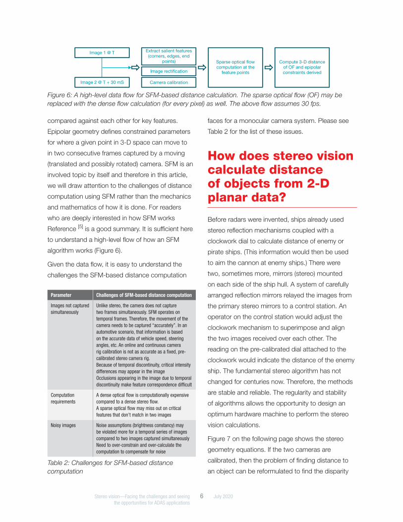
compared against each other for key features.

Epipolar geometry defines constrained parameters

for where a given point in 3-D space can move to

in two consecutive frames captured by a moving

(translated and possibly rotated) camera. SFM is an

involved topic by itself and therefore in this article,

we will draw attention to the challenges of distance

computation using SFM rather than the mechanics

and mathematics of how it is done. For readers

who are deeply interested in how SFM works

Reference [5] is a good summary. It is sufficient here

to understand a high-level flow of how an SFM

algorithm works (Figure 6).

Given the data flow, it is easy to understand the

challenges the SFM-based distance computation

Parameter Challenges of SFM-based distance computation

Images not captured simultaneously

Unlike stereo, the camera does not capture two frames simultaneously. SFM operates on temporal frames. Therefore, the movement of the camera needs to be captured “accurately”. In an automotive scenario, that information is based on the accurate data of vehicle speed, steering angles, etc. An online and continuous camera rig calibration is not as accurate as a fixed, pre-calibrated stereo camera rig. Because of temporal discontinuity, critical intensity differences may appear in the image Occlusions appearing in the image due to temporal discontinuity make feature correspondence difficult

Computation requirements

A dense optical flow is computationally expensive compared to a dense stereo flow. A sparse optical flow may miss out on critical features that don’t match in two images

Noisy images Noise assumptions (brightness constancy) may be violated more for a temporal series of images compared to two images captured simultaneously Need to over-constrain and over-calculate the computation to compensate for noise

Table 2: Challenges for SFM-based distance computation

faces for a monocular camera system. Please see

Table 2 for the list of these issues.

How does stereo vision calculate distance of objects from 2-D planar data?

Before radars were invented, ships already used

stereo reflection mechanisms coupled with a

clockwork dial to calculate distance of enemy or

pirate ships. (This information would then be used

to aim the cannon at enemy ships.) There were

two, sometimes more, mirrors (stereo) mounted

on each side of the ship hull. A system of carefully

arranged reflection mirrors relayed the images from

the primary stereo mirrors to a control station. An

operator on the control station would adjust the

clockwork mechanism to superimpose and align

the two images received over each other. The

reading on the pre-calibrated dial attached to the

clockwork would indicate the distance of the enemy

ship. The fundamental stereo algorithm has not

changed for centuries now. Therefore, the methods

are stable and reliable. The regularity and stability

of algorithms allows the opportunity to design an

optimum hardware machine to perform the stereo

vision calculations.

Figure 7 on the following page shows the stereo

geometry equations. If the two cameras are

calibrated, then the problem of finding distance to

an object can be reformulated to find the disparity

Image 2 @ T + 30 mS

Image 1 @ T Extract salient features(corners, edges, end

points) Sparse optical flowcomputation at the

feature points

Compute 3-D distanceof OF and epipolarconstraints derivedImage rectification

Camera calibration

Figure 6: A high-level data flow for SFM-based distance calculation. The sparse optical flow (OF) may be replaced with the dense flow calculation (for every pixel) as well. The above flow assumes 30 fps.


between the simultaneous images captured by

the left and right cameras for that point. For pre-

calibrated stereo cameras, the images could

be rectified such that epipolar geometrical lines

are simple horizontal searches (on the same

row) for every point between two images. The

disparity is then defined as the number of pixels

a particular point has moved in the right camera

image compared to the left camera image. This

concept is crucial to remember, since it allows

regular computation patterns that are amenable for

hardware implementation. Before we delve deeper

into this topic, the concept of disparity needs to be

clarified further.

Stereo disparity calculation and accuracy of calculated distance

Figure 8 shows three different graphs to

demonstrate the relationship between disparity

and the distance-to-object. The first thing to

notice is that the measured disparity is inversely

proportional to the distance of an object. The

closer an object is to the stereo cameras; more

is the disparity and vice-versa. Theoretically, a

point with zero disparity is infinitely away from the

cameras. Concretely, the calculation shows that

for the chosen physical parameters of the system

(see Figure 8-a), a disparity of 1 pixel implies a

distance of ~700 meters, while for a calculated

disparity of 2 pixels, the estimated distance is ~350

meters. That is a really large resolution and if the

disparity calculation is inaccurate by one pixel,

then the estimated distance will be incorrect by a

large amount (for longer distances > 100 meters).

For shorter distances (lower part of the curves in

Figure 8 < 50 meters), the resolution of distance

calculation is much more improved. It is evident

by the distance calculation points in the graphs

T

P = (X, Y, Z)

pl

= (xl,y

l) p

r= (x

r,y

r)

Ol

Or

Y

X

f f

Stereo geometry equationsx

l= f * X/Z ……. (1)

xr= f * (T–X)/Z …(2)

(1) – (2) Z = fT/(xl–x

r), if d = x

l–x

r

Y = ylT / d

X = xlT / d

Z

Figure 7: Stereo geometry equations. The depth of a point in 3-D space is inversely proportional to the disparity of that point between the left and right cameras. [6]

800.0

700.0

600.0

500.0

400.0

300.0

200.0

100.0

0.0

800.0

700.0

600.0

500.0

400.0

300.0

200.0

100.0

0.0

800.0

700.0

600.0

500.0

400.0

300.0

200.0

100.0

0.0

0 0 010 10 1020 20 2030 30 3040 40 4050 60 6050 50

Dis

tan

ce

Dis

tan

ce

Dis

tan

ce

Disparity

(a)

Disparity

(b)

Disparity

(c)

Distance (meters) vs. Disparity (pixels)

Full pixel accuracy


Half pixel accuracy


Quarter pixel accuracy

Figure 8: Distance vs. disparity graphs for different accuracy of calculation. The distance accuracy improves with increased pixelar accuracy of disparity calculation. Calculations made for (a) 30-cm distance between two cameras, (b) focal length of 10 mm, (c) pixel size of 4.2 microns.


which crowd together. In this range, if the disparity

calculation is inaccurate by one pixel (or less), the

calculated distance is wrong by approximately two

to three meters.

There are methods to improve the accuracy of the

system further. As shown by Figures 8(b) and 8(c),

if the disparity calculation is performed at half or

quarter pixel levels, then the resolution of distance

calculation improves proportionally. In those

scenarios, for distances larger than 100 meters (but

less than 300 meters), the resolution of calculated

distance for consecutive disparity increase is ~30–

40 meters. For distances smaller than 100 meters,

the accuracy can be better than 50 cms. It may be

important to reiterate that the accuracy needs to

be maximized (preferable to < 0.1 meters range)

for a collision avoidance system operating for close

distances. At the same time, operating range of the

stereo camera needs to be improved, even at the

cost of slight loss to accuracy if needed.

The range of the stereo camera ADAS system

If you see the basic stereo equation (Figure 7)

once again, then it is evident that to improve

the maximum range of the system, the distance

computation needs to be reasonably accurate for

low disparities. That can be achieved by any of the

following three methods. Each of these methods

have associated trade offs for mechanical or

electronic design and eventually system cost.

(a) Use a smaller pixel size ® If we use a smaller

pixel size (let’s say half), and if everything else

stays the same, the range improves by about

50 percent (for the same accuracy)

(b) Increase the distance between the two

cameras ® If “T” is increased to double, and

if everything else stays the same, the range

improves by about 50 percent (for the same

accuracy)

(c) Change the focal length ® If “f” is increased

to double, and if everything else stays the

same, the range improves by about 50

percent (for the same accuracy), but field of

view narrows down

(d) Use a computation system that calculates

stereo disparity with sub-pixel accuracy

Although mathematically feasible, options (b) and

(c) have a direct bearing on the physical attributes

of the system. When a stereo system needs to

be mounted in a car, typically it will have a fixed

dimension or the requirement for the system

to be as small as possible. This aesthetic need

goes against increasing the distance between the

cameras (T) or the focal length (f). Therefore, most

practical options for an accurate stereo distance

calculation system with high range and accuracy

revolve around options (a) and (d) above.

The process

Figure 9 on the following page shows the high-level

block diagram for data flow and compute chains

to calculate the stereo disparity. Please note the

absence of the camera calibration step that was

present in the SFM block diagram in Figure 6, and

that there is no need to search for features in the

dense stereo disparity algorithm either. Identifying

features and objects is required for SFM-based

distance calculation methods that compute distance

based on the size of an object.

The image rank transformation is most often the

first or second step in the stereo image processing

pipe. The purpose of this step is to ensure that


the subsequent block comparisons between two

images are robust to real-world noise conditions

such as illumination or brightness changes between

the left and right images [7]. These changes can be

caused by many factors. Some of these include

different illumination because of varied points of

view from the two cameras and slight differences

between the shutter speeds and other jitter artifacts

that may cause the left and right images to be

captured at slightly different points of time by

the cameras.

There are various papers and approaches

suggested by researchers for different rank

transform options for images and how they impact

the robustness of disparity calculations [8]. The

image rectification step in Figure 9 ensures that the

subsequent disparity calculation can be performed

along the horizontal epipolar search lines. The

next steps in the process are actual calculation of

disparity, confidence levels of the computation and

post processing. The dense disparity calculation

is mostly performed in spatial domain although

there are some approaches suggested to calculate

disparity in frequency domain [9].

These approaches attempt to take advantage of the

fact that large FFTs can be calculated comparatively

quickly, yet there are other complications involved

in FFT that don’t tilt the balance in its favor yet.

Without the need to go deeper into that discussion

in this article, it is a fair claim that most (if not

all) productized stereo disparity algorithms are

implemented in spatial domain. At the most basic

level, this analysis requires that for every pixel in the

left (transformed) image, we need to pick a small

block of pixels surrounding it.

Next, we need to search in the right side

(transformed) image along the epipolar (horizontal)

line until finding where the same block is located.

This computation is performed for every possible

value of disparity (from one to the maximum—64

or 128 or any other value). The difference (or cross

correlation) between the left and right side block

will approach minima (maxima) close to the actual

value of disparity for the pixel. The performed

“moving-window” block comparison and matching

will calculate how much the block has moved,

and the result will be used to calculate distance of

that particular pixel in 3-D space. This process is

shown in Figure 10. One such example of disparity

calculation using rank transform followed by sum

of absolute differences (SAD) based cost function

minimization is given in [8].

Image right

Image left

Image rectification(To enable

horizontal epipolarsearches)

Postprocess

Computedistancefor every

pixel

Calculate disparity andconfidence levels forevery pixel (dense)

Image rank

Image rank

Figure 9: A high-level data and algorithm flow for stereo disparity-based distance computation.

Figure 10: Simple SAD-based block-comparison algorithm for finding disparity.

Shift block and compare in the right image for best match

Best match = disparity for pixel

Repeat calculation for every pixel in left image

For every possible value of disparity in right image


The SAD-based approach for finding disparity is

elegant and sometimes too simplistic. The basic

premise of this approach is that for a given block

of pixels, the disparities are equal, however this is

almost never true at the edges of the objects. If

you review Figure 2 again and pay attention to the

annotations made for forks of the motor cycle and

the red box, you would quickly realize that there

will be many adjacent pixels where disparity will

be different. It is indeed normal since the “red box

on the shelf” is about two meters farther from the

camera than the “forks”. The disparity for a small

block of pixels may change drastically at object

boundaries and marginally for slanted or curved

surfaces. The “cones and faces” image from

Middlebury dataset [10] highlights this fact perfectly.

The adjacent pixels found over one cone (slightly

slanted surface) will have minor disparity changes,

while the object boundaries will have large disparity

differences. Using a simple SAD-based algorithm

along with rank transform will leave large disparity

holes on both occlusions such as the artifacts

that are visible only in one camera and object

boundaries.

To resolve such inaccuracies with deterministic run

time, an elegant approach was suggested by [11].

This approach is called “semi global matching”.

In this approach, a smoothness cost function is

calculated for every pixel in more than one direction

(4, 8 or 16). The cost function calculation is shown

in Figure 12 below. The objective is to optimize the

cost function S(p,d) in multiple directions for every

pixel and to ensure a smooth disparity map. The

original paper for SGM suggested 16 directions for

optimization of the cost function, though practical

implementations have been attempted for 2, 4 and

8 directions as well.

A concrete implementation of SGM cost functions

and optimization algorithm is shown in Figure 13 on

the following page. With this pseudo-code segment,

it is easy to assess the memory, computation and

Figure 11: Cones and faces from Middlebury dataset. The disparity calculation is performed using simple SAD. The disparity keeps changing marginally on the curved surfaces, while it changes drastically on the object boundaries. See the disparity holes in the fence on the top-right, other object discontinuities and occlusions on left border.

Left Right Disparity map

Figure 12: Optimization cost function equations for SGM.


eventually hardware complexity requirements to

enable SGM-based computation in real time.

Computation and memory requirements for the disparity calculation

As you can well imagine, this calculation is

compute heavy for ADAS applications. A typical

front-facing stereo camera rig is a set of 1-Mpixel

cameras operating at 30 frames per second. The

first steps in the disparity calculation process are

rank transforms. A typical rank transform is a

census transform or a slightly modified version.

The inputs required are both stereo images, while

the outputs are census-transformed image pairs.

The computation required for census transform

for an N×N block around the pixel is to perform

60 million, N×N census transforms. Every census

transform done for a pixel over a N×N block

requires N2 comparison operations. Some other

involved rank transforms need an N2 point sort for

every pixel. It is safe to assume that the minimum

possible requirement is to run 60 million × N2

comparison operations for rank transformation in

practical systems deployed on real vehicles for next

few years.

The second step in the process requires image

rectification to ensure that the epipolar disparity

searches are needed on the horizontal lines. The

third step is more interesting since It involves

calculation of C(p,d), Lr(p,d) and S(p,d) for every

pixel and disparity combination (see Figure 13).

If C(p,d) is a block-wise SAD operation and the

block size is N×N, the required system range

is ~200 meters and the accuracy of distance

calculated required half-pixel disparity calculation

then the system will require to calculate C(p,d) for

64–128 disparity possibilities. The total compute

requirements for C(p,d) with these parameters are

to perform 60 million × N2 × 128 SAD operations

every second.

The calculation of Lr(p,d) needs to be done for every

pixel in “r” possible directions, hence the calculation

of this term (see Figure 13) needs to be done 60

million × 128 × r times. The calculation for one pixel

requires five additions (if you consider subtraction

a special form of addition) and one minima-finding

operation. Putting it together, the calculation of

Lr(p,d) per second needs 60 million × 128 × r

× 5 additions and 60 million × 128 × r minima

computations for four terms.

Figure 13: Pseudo code for implementation of SGM.

8 1

3 0

7 1

4 0

3 0

Pixel values Census

6 1

6 1

5 14 T T = 11011001

8 5

3 0

7 4

4 1

3 0

Pixel values Pixel rank

6 3

6 3

5 24 1 T = 5,4,0,2,1,3,0,1,3

Figure 14: Rank transform examples for images. The left part of the image is simple census transform. The right half is called “complete rank transform” [7].


The calculation of S(p,d) needs to be done r times

for every possible pixel and disparity value, every

computation of S(p,d) requires “r” additions and

one comparison. The total operations needed for

calculating this per second are 60 million × 128 × r

additions and 60 million × 128 comparisons.

Putting all three together, an accurate SGM-

based disparity calculation engine, running

on 1 Mpixel, 30-fps cameras and intending to

calculate 128 disparity possibilities will need to

perform approximately 1 Tera operations (additions,

subtractions, minima finding) every second. To put

this number in perspective, advanced general-

purpose processors in embedded domain issue

seven to ten instructions per cycle. Some of these

instructions are SIMD type, i.e., they can tackle

8–16 pieces of data in parallel. Considering the

best IPC that a general-purpose processor has to

offer, a quad-core processor running at 2 GHz will

offer about 320 Giga 64-bit operations. Even if we

consider that most of the stereo pipeline will be 16

bits and the data can be packed in 64-bit bins with

100 percent efficiency, a quad-core general-purpose

processor is hardly enough to meet the demands

of a modern day ADAS stereo vision system. The

objective of a general-purpose processor is to

afford high-level programmability of all kinds. What

it means is that designing a real-time ADAS stereo

vision system requires specialized hardware.

Robustness of calculations

The purpose of ADAS vision systems is to avoid

or at least minimize the severity of road accidents.

More than 1.2 million people are killed every year

due to road accidents, making it the leading cause

of death for people aged 15–29 years. Pedestrians

are the most vulnerable road users, with more

than 250,000 pedestrians succumbing to injuries

each year. The major cause of road accidents is

mistakes made by drivers either due to inattention

or fatigue. Therefore, the most important purpose

of an ADAS vision system for emergency braking

is to reduce the severity and frequency of the

accidents. That is a double-edged requirement

since a vision system not only has to estimate the

distances correctly with high robustness every

video frame and every second, but also minimize

the false positive scenarios. To ensure the ADAS

system is specified and designed for the right

level of robustness, ISO 26262 was created as

an international standard for the specification,

design and development of electronics system for

automotive safety applications.

A little calculation here will bring out the estimated

errors in computing distance for a stereo vision

system. Please see Figure 15. If the error tolerances

for the focal length (f) and the distance between

the cameras (T) is 1 percent and the accuracy of

disparity calculation algorithm is 5 percent, then

the calculated distance (Z) will still be about 2.5

percent inaccurate. Improving the accuracy of the

disparity calculation algorithm to a sub-pixel (quarter

or half pixel) level therefore is important. This has

two implications. The first being increased post-

processing interpolation compute requirements

of the algorithm and the hardware. The second

requirement is more sophisticated and is related to

ISO 26262.

Z=f T/dIf f, T & calculated d have a standard deviation of s , s & s

respectively, then

s = ((s ) + (s ) + (s ) )

f T d

Z d T f2 2 2 1/2

Figure 15: Statistical error estimation for calculated distance by a stereo vision system [13].


The architecture and design needs to ensure

that both transient and permanent errors in the

electronic components are detected and flagged

within the fault tolerant time interval (FTTI) of the

system. The calculation of FTTI and the other

related metrics is beyond the scope of this article,

yet it should suffice to point out that the electronic

components used to build the system need to

enable achieving the required ASIL levels for the

ADAS vision system.

System hardware options and summary

In this article, we reviewed the effectiveness of

various algorithm options in general and stereo-

vision algorithms in particular to calculate distance

for an automotive ADAS safety emergency

braking system. Texas Instruments is driving

deep innovation in the field of ADAS processing

in general, and efficient and robust stereo-vision

processing in particular.

There can be many different electronic system

options to achieve the system design and

performance objectives for an ADAS safety vision

system. Heterogeneous chip architectures by Texas

Instruments (TDA family) are suitable to meet the

performance, power, size and ASIL functional safety

targets for this particular application. A possible

system block diagram for stereo and other ADAS

systems using TI TDA2x and TDA3x devices and

demonstrations of the technology are available at

www.ti.com/ADAS.

References[1] Cave paintings: http://en.wikipedia.org/wiki/

Cave_painting#Southeast_Asia

[2] D. Scharstein, H. Hirschmüller, Y. Kitajima, G.

Krathwohl, N. Nesic, X. Wang, and P. Westling.

“High-resolution stereo datasets with

subpixel-accurate ground truth”. In German

Conference on Pattern Recognition (GCPR 2014),

Münster, Germany, September 2014

[3] Figure credit: “Vision-based Object Detection and

Tracking”, Hyunggic!, http://users.ece.cmu.

edu/~hyunggic/vision_detection_tracking.

html

[4] Image credit: pixabay.com

[5] 3D Structure from 2D Motion, http://www.

cs.columbia.edu/~jebara/papers/sfm.pdf

[6] Chapter 7 “Stereopsis” of the textbook of E.

Trucco and A. Verri, Introductory Techniques for

3-D Computer Vision, Prentice Hall, NJ, 1998 and

lecture notes from https://www.cs.auckland.

ac.nz/courses/compsci773s1t/lectures/

773-GG/topCS773.htm

[7] “The Complete Rank Transform: A Tool for

Accurate and Morphologically Invariant Matching

of Structures”, Mathematical Image Analysis

Group, Saarland University, http://www.mia.

uni-saarland.de/Publications/demetz-

bmvc13.pdf

[8] “A Novel Stereo Matching Method based on Rank

Transformation”, Wenming Zhang , Kai Hao*,

Qiang Zhang, Haibin Li Reference:

http:// ijcsi.org/papers/IJCSI-10-2-1-39-44.pdf

[9] “FFT-based stereo disparity estimation for stereo

image coding”, Ahlvers, Zoelzer and Rechmeier

http://en.wikipedia.org/wiki/Cave_painting#Southeast_Asia

http://en.wikipedia.org/wiki/Cave_painting#Southeast_Asia

http://www.cs.middlebury.edu/~schar/papers/datasets-gcpr2014.pdf

http://www.cs.middlebury.edu/~schar/papers/datasets-gcpr2014.pdf

http://www.ti.com/lit/ug/sprugs2c/sprugs2c.pdf

http://users.ece.cmu.edu/~hyunggic/vision_detection_tracking.html



http://www.pixabay.com

http://www.cs.columbia.edu/~jebara/papers/sfm.pdf

http://www.cs.columbia.edu/~jebara/papers/sfm.pdf

https://www.cs.auckland.ac.nz/courses/compsci773s1t/lectures/773-GG/topCS773.htm



http://www.mia.uni-saarland.de/Publications/demetz-bmvc13.pdf



http://ijcsi.org/papers/IJCSI-10-2-1-39-44.pdf

[10] “Semi-Global Matching”,

http://lunokhod.org/?p=1356

[11] “Accurate and Efficient Stereo Processing by

Semi-Global Matching and Mutual Information”,

https://ieeexplore.ieee.org/

document/1467526

[12] “More than 270,000 pedestrians killed on roads

each year”, http://www.who.int/

mediacentre/news/notes/2013/

make_walking_

safe_20130502/en/

[13] “Propagation of Error”, http://chemwiki.

ucdavis.edu/Analytical_Chemistry/

Quantifying_Nature/Significant_Digits/

[14] Optical flow reference: “Structure from

Motion and 3D reconstruction on the easy

in OpenCV 2.3+ [w/ code]” http://www.

morethantechnical.com/2012/02/07/

structure-from-motion-and-3d-

reconstruction-on-the-easy-in-opencv-2-3-

w-code/

[15] Mutual information reference: “Mutual

Information as a Stereo Correspondence

Measure”, http://repository.upenn.edu/cgi/

viewcontent.cgi?article=1115&context=cis_

reports

[16] Image entropy analysis using Matlab®

[17] Image credit: “Engines idling in New York despite

law”, CNN News, http://www.cnn.com/

2012/02/06/health/engines-new-york-law/

SPRY300A© 2020 Texas Instruments Incorporated

Important Notice: The products and services of Texas Instruments Incorporated and its subsidiaries described herein are sold subject to TI’s standard terms and conditions of sale. Customers are advised to obtain the most current and complete information about TI products and services before placing orders. TI assumes no liability for applications assistance, customer’s applications or product designs, software performance, or infringement of patents. The publication of information regarding any other company’s products or services does not constitute TI’s approval, warranty or endorsement thereof.

The platform bar is a trademark of Texas Instruments. All other trademarks are the property of their respective owners.

http://lunokhod.org/?p=1356

http://www.who.int/mediacentre/news/notes/2013/make_walking_safe_20130502/en/



http://chemwiki.ucdavis.edu/Analytical_Chemistry/Quantifying_Nature/Significant_Digits/Propagation_of_Error



http://www.morethantechnical.com/2012/02/07/structure-from-motion-and-3d-reconstruction-on-the-easy-in-opencv-2-3-w-code/





http://repository.upenn.edu/cgi/viewcontent.cgi?article=1115&context=cis_reports



http://www.cnn.com/2012/02/06/health/engines-new-york-law/

http://www.cnn.com/2012/02/06/health/engines-new-york-law/

https://ieeexplore.ieee.org/document/1467526

IMPORTANT NOTICE AND DISCLAIMER

TI PROVIDES TECHNICAL AND RELIABILITY DATA (INCLUDING DATASHEETS), DESIGN RESOURCES (INCLUDING REFERENCE DESIGNS), APPLICATION OR OTHER DESIGN ADVICE, WEB TOOLS, SAFETY INFORMATION, AND OTHER RESOURCES “AS IS” AND WITH ALL FAULTS, AND DISCLAIMS ALL WARRANTIES, EXPRESS AND IMPLIED, INCLUDING WITHOUT LIMITATION ANY IMPLIED WARRANTIES OF MERCHANTABILITY, FITNESS FOR A PARTICULAR PURPOSE OR NON-INFRINGEMENT OF THIRD PARTY INTELLECTUAL PROPERTY RIGHTS.These resources are intended for skilled developers designing with TI products. You are solely responsible for (1) selecting the appropriate TI products for your application, (2) designing, validating and testing your application, and (3) ensuring your application meets applicable standards, and any other safety, security, or other requirements. These resources are subject to change without notice. TI grants you permission to use these resources only for development of an application that uses the TI products described in the resource. Other reproduction and display of these resources is prohibited. No license is granted to any other TI intellectual property right or to any third party intellectual property right. TI disclaims responsibility for, and you will fully indemnify TI and its representatives against, any claims, damages, costs, losses, and liabilities arising out of your use of these resources.TI’s products are provided subject to TI’s Terms of Sale (www.ti.com/legal/termsofsale.html) or other applicable terms available either on ti.com or provided in conjunction with such TI products. TI’s provision of these resources does not expand or otherwise alter TI’s applicable warranties or warranty disclaimers for TI products.

Mailing Address: Texas Instruments, Post Office Box 655303, Dallas, Texas 75265Copyright © 2020, Texas Instruments Incorporated

http://www.ti.com/legal/termsofsale.html

http://www.ti.com

Documents

Stereo vision- facing the challenges and seeing the