Embed Size (px)
Citation preview

COPYRIGHT NOTICE:
Stephen P. Ellner and John Guckenheimer: Dynamic Models in Biology
is published by Princeton University Press and copyrighted, © 2006, by Princeton University Press. All rights reserved. No part of this book may be reproduced in any form by any electronic or mechanical means (including photocopying, recording, or information storage and retrieval) without permission in writing from the publisher, except for reading and browsing via the World Wide Web. Users are not permitted to mount this file on any network servers.
Follow links for Class Use and other Permissions. For more information send email to: [email protected]

January 18, 2006 16:07 m26-main Sheet number 305 Page number 283
9 Building Dynamic Models
Modeling is often said to be more of an art than a science, but in some ways it is
even more like a professional trade such as carpentry. Each modeler will approach
a problem somewhat differently, influenced by their training, experience, and
what happens to be fashionable at the moment. But given a set of specifications—
what is it for, what data are available, and so on—two experienced modelers are
likely to use similar methods and to produce functionally similar final products. The goal of this chapter is to outline the modeling process and introduce some
tools of the trade. Such generalities can get to be dry, but we hope that by now
you are tempted to do some modeling on your own—or perhaps you are required
to do some—so you will tolerate some words of advice. Much of this chapter is concerned with connecting models and data—a sub-
ject called statistics. Nonetheless, contacts have been limited between the sta-tistical research community and the scientific communities where dynamic
models are used, such as economics and engineering—so limited that many
other fields have independently developed statistical methods specific to their
needs. Biologists seemingly have no such need—the specialty areas of bio-statistics and statistical genetics are recognized in mainstream statistics—but there is very little on dynamic models in the mainstream statistics literature
or curriculum. An online search in June 2005 using search engines at journal home pages, JSTOR (http://www.jstor.org), and the Current Index of Statistics
(http://www.statindex.org) found two papers concerning a differential equation
model in the last ten years of the Journal of the American Statistical Association, four in the last ten years of Biometrics, and five in the last ten years of Biometrika, which is under 1
2 % of the total for those journals over the same time period. Our
bookshelves hold any number of statistics textbooks, elementary and advanced, with one or (usually) fewer applications to a differential equation model. The
reverse is also true—one can get a Ph.D. in mathematical or computational biol-ogy without any formal training in statistics, so very few dynamic modelers are
aware of how modern computer-intensive statistical methods can be applied to
dynamic models.

January 18, 2006 16:07 m26-main Sheet number 306 Page number 284
284 Chapter 9
This chapter reflects our belief that the next generation of dynamic model-ers should not perpetuate the historical trend of treating statistical and dynamic
modeling as two separate fields of knowledge, one of which can be left to some-body else. Connecting models with data is almost always the eventual goal. Taking the time to learn statistical theory and methods will make you a better
modeler, and a more effective collaborator with experimental biologists. Reading
this chapter is only a beginning.
9.1 Setting the Objective
Figure 9.1 outlines the steps involved in developing, evaluating, and refining a
dynamic model. We will now proceed through them one by one. The first, essential, and most frequently overlooked step in modeling is to de-
cide exactly what the model is for. We cannot ask models to be literally true, but we can insist that they be useful, and usefulness is measured against your
objectives and the value of those objectives. One important aspect of setting objectives is to decide where they fall on the
continuum between theoretical and practical modeling (Chapter 1). That is, will you use the model to help you understand the system and interpret observations
of its behavior, or to predict the system, running either on its own or with outside
interventions? Another important decision is how much numerical accuracy
you need. Accurate prediction is often the primary goal in practical applications. But if theoretical understanding is the major goal, it may be good enough if the model gets the sign right or in some other way gives a reasonable qualitative
match (treatment A really had a larger effect than treatment B; the system really
does oscillate rather than settling down to an equilibrium; etc.). The next step is to assess the feasibility of your goals. The most common
constraints are time and data. Some pessimism about time requirements is usually
a good idea, especially for beginners—such as students doing a term project. It is usually a good idea to start with a small project that can later be expanded to
a more complete model, or a simple model to which more detail can be added
later. In contrast, assessment of whether the available data will meet your needs
should be optimistic. Beginners frequently decide that a project cannot be done
because some “crucial” piece of information is missing. But models often have
several parameters or assumptions that have little or no impact on relevant as-pects of model behavior. The only way to find out if the data you are missing are
actually needed is to build the model, and then do a sensitivity analysis (Chapter
8) to find out which parts really matter. If you seem to have most of the data that you need, the odds are good that you or an experienced advisor can find some
way of working around the gaps.

January 18, 2006 16:07 m26-main Sheet number 307 Page number 285
∑ ∑
285 Building Dynamic Models
Figure 9.1 Outline of the modeling process.
9.2 Building an Initial Model
Figure 9.2 summarizes the steps in building a dynamic model. As our main exam-ple we will use continuous-time compartment models, because they are widely
used and allow us to present the main ideas and methods with a minimum of terminology and notation.
Recall from Chapter 1 that the state variables of a compartment model are the
amounts of a single kind of “stuff” in a number of locations or categories. The
dynamic equations are
n n
dxi /dt = ρij (t) − ρji (t ) [9.1] j=0 j=0j =i j =i
where xi(t ) is the amount in compartment i at time t , and ρij(t) is the flow rate
from compartment j to compartment i at time t , with compartment 0 being the
“outside”—the part of the world beyond the limits of the model. Note that there

January 18, 2006 16:07 m26-main Sheet number 308 Page number 286
286 Chapter 9
Figure 9.2 Outline of the steps in developing a model.
is no x0 because the “outside world” is not part of the model. By convention, compartment models are written so that mass is conserved. If any new stuff is
created within the system (e.g., births of new susceptibles in an epidemic model), it is represented as an input from the outside. If any stuff is destroyed (e.g., deaths
of infected individuals), this is represented as a loss to the outside. By using a deterministic model with continuous state variables, we are im-
plicitly assuming that many individual units of the stuff are flowing through the
system. Equation [9.1] cannot be applied to (say) five atoms of a trace metal mov-ing through the body, since for each compartment we could only have xi = 1, 2, 3, 4, or 5. Another assumption is that each compartment is well mixed, meaning
that all individual units within the same compartment are identical, regardless
of their past history or how long they have been in the compartment. Without this assumption, the xi by themselves would not completely describe the state
of the system. In the terminology of the last chapter, a compartment model is
based on an agent-based model where each agent has a finite number of possible
states. Equation [9.1] is then the mean field equation for the expected changes
in the numbers of agents in each possible state.
9.2.1 Conceptual Model and Diagram
A model begins with your ideas about which variables and processes in the sys-tem are the most important. These may come from hard data and experimental

January 18, 2006 16:07 m26-main Sheet number 309 Page number 287
287 Building Dynamic Models
evidence, or they may be hypotheses that are being entertained for the moment, in order to determine their consequences.
A useful first step in turning these concepts into a dynamic model is to represent the conceptual model as a diagram showing the state variables and processes. Compartment models can be depicted in a compartment diagram consisting of a labeled or numbered box for each compartment, and an arrow for each flow
(each nonzero ρij). As you draw the boxes and arrows, you are formalizing the
conceptual model by choosing which components and processes are included, and which are outside the model—either ignored, or included in the external environment in which your model operates.
A good strategy for turning verbal concepts into a diagram is to start with the
phenomena or data that figure explicitly in your objectives, and then work out from there until you are willing to declare everything else “outside.”
• Quantities “inside” that will change over time as your model is run are your state
variables.
• Quantities “outside” that change over time are called exogenous variables or
forcing functions. They are taken as given, and only modeled descriptively (e.g.,
how temperature changes over a day or rainfall varies over the year; the rate at
which bone marrow produces new T-cells that enter the blood stream).
• Quantities that do not change over time are called parameters.
Diagramming a model forces you to decide which processes require mechanis-tic description in order to accomplish your objectives. If it is enough for your
purposes to know how a variable changes over time without knowing why, you
can put it outside the model as an exogenous variable. More and more variables
often move “outside” as a model is developed. Another issue is choosing the level of detail. In a compartment model this is
determined by the number of compartments, because units within a compart-ment are treated as identical, even though they usually are not. This is called
aggregation, and causes aggregation error—treating things that really are different as if they were the same. For example,
• Species are combined into broad categories: birds, grasses, bacteria, etc.
• Physical location is often ignored: one bone versus another in the skeleton,
location of a virus particle in the bloodstream, location of infected individuals.
• Compartments are often used to subdivide a continuum. Models of reproducing
cell populations sometimes assume there are only a few discrete types of cells (e.g.,
distinguished by their stage of the cell cycle). Epidemic models often classify
infected individuals as exposed (not contagious) versus infected (contagious),
whereas there is actually a gradual transition. Space is often modeled as a grid of
discrete cells, with variables allowed to differ between cells but not within them

January 18, 2006 16:07 m26-main Sheet number 310 Page number 288
288 Chapter 9
(the reverse is also done, i.e., a tissue composed of discrete cells may be
approximated as a uniform continuum for the sake of simplicity in theoretical
models).
Useful models may have widely differing levels of aggregation, depending on
the questions being asked, for example:
• Carbon in humans. A model of glucose metabolism in the human body (Cramp and
Carson 1979) had nearly fifty different compartments, including eleven for
different substances in the liver. Their “simplified” model recognized six different
compartments for glucose in the body: (1) intestinal tract; (2) hepatic portal; (3)
and (4) two forms in the liver; (5) blood; (6) “peripheral tissue.” To model carbon
flow in the Aleutian Island ecosystem, Hett and O’Neill (1974) used nine highly
aggregated compartments, such as (1) atmosphere; (2) land plants; (3) man; (4)
marine animals and zooplankton; and so on. The object was to see which
pathways of carbon flow were most critical to the indigenous human population.
This model ignores location, aggregates species, and instead of six or fifty
compartments for the glucose in one human there is one compartment for all
forms of carbon in all Aleut humans.
• Carbon in soils. The initial version of the CENTURY model for soil organic matter
(SOM) used eight compartments as shown in Figure 9.3, but represented soil by a
single layer (Parton et al. 1987, 1988). The current version (NREL 2001) allows for a
vertically layered soil structure (so each SOM compartment is replicated multiple
times), simulates C, N, P, and S dynamics, includes models for several different
vegetation types (grassland/crop, forest or savanna), and can simulate agricultural
management actions such as crop rotation, fertilization, and grazing. Currently,
most global ecosystem models use soil carbon and nutrient modules that closely
follow the basic CENTURY model (Bolker et al. 1998). In contrast, a global climate
model developed by the U.K. government’s Meteorological Office (Cox et al. 2000)
uses just one compartment for the total amount of organic matter in a unit of area
under a given type of vegetation (five vegetation types are recognized: broadleaf
and coniferous trees, shrubs, C3 and C4 grasses). The overall model also includes
oceanic and atmospheric components, and operates at the global scale by dividing
the earth surface into a large number of grid cells. The model for vegetation/soil
dynamics within each cell was kept simple so that all model components could be
simulated simultaneously to represent dynamic climate-vegetation feedbacks (Cox
2001).
Overaggregation leads to errors if the units within a compartment are het-erogenous in their behavior. Then no valid set of rate equations can be written, because a count of the total number in each compartment is not sufficient infor-mation for predicting what happens next. For other types of models, the equiv-

January 18, 2006 16:07 m26-main Sheet number 311 Page number 289
289 Building Dynamic Models
litter
metabolic litter
Soil
litter
Soil metabolic litter
microbes
Soil microbes
SOM
SOM
Surface structural
Surface
structural
Surface
(fast SOM)
(fast SOM)
Slow
Passive
Figure 9.3 Diagram of the compartments for soil organic matter in the CENTURY
model (from Bolker et al. 1998). The dotted arrow (from the passive to the slow
pool of decomposing organic matter in the soil) represents a very small flow.
alent of aggregation is to ignore variables whose effect is assumed to be relatively
unimportant—for example, quantities that really vary over time or space are as-sumed to be constant. In the fishpond model of Chapter 1, the state variables
for phytoplankton represent the total abundance of several species—because one
species always made up about 90% of the phytoplankton biomass, variation in
which species made up the remaining 10% was simply ignored. You can also get into trouble by including too much detail. Biologists often
feel that adding more and more biological detail will make a model more accu-rate, but that is true only up to a point if parameters are estimated from data. More detail requires more parameters, so the number of observations going into
each parameter goes down, and eventually all parameter estimates are unreliable. Conceptually,
Prediction error = Model error + Parameter error. [9.2]
(In practice there also are numerical errors in computing model solutions, but that is a separate issue.) Model error is error in predictions due to the fact that

January 18, 2006 16:07 m26-main Sheet number 312 Page number 290
290 Chapter 9
your model is not an exact representation of reality. Parameter error is error in
predictions due to the fact that parameters values estimated from data are not the optimal ones for maximizing the model’s prediction accuracy.
The best level of detail for making numerically accurate predictions strikes a
balance between model error and parameter error. Consequently, the model with the lowest prediction error is often one that deliberately makes simplifying
assumptions that contradict known biology. For example, Ludwig and Walters
(1985) compared two models used for regulating commercial fishing effort:
1. The traditional simple Ricker model uses a single variable for the fish population,
B(t ) = total fish biomass in year t . Changes in B(t) are determined by the fishing
effort in year t , E(t), and the resulting harvest H (t):
−qE(t)),H (t ) = B(t)(1 − e
S(t ) = B(t) − H (t), [9.3]
B(t + 1) = r(t )S(t )eα−βS(t ).
The first line of [9.3] specifies how increasing fishing effort E(t) leads to a larger
fraction of the biomass B(t) being harvested. S(t) is then the remaining
unharvested “stock,” which (in the last line) produces next year’s population via
survival and reproduction.
2. The “structured” model uses a full matrix population model for the stock. Only
adults are harvested—which is true but omitted by the Ricker model—using the
same equation for H (t) as the Ricker model.
The manager’s assumed goal is to choose E(t) to maximize the long-run rate of economic return from the harvest. The available data in year t are the fishing
effort and harvest in prior years, from which the parameters of each model need
to be estimated. The fitted model is then used to set the fishing effort. Ludwig
and Walters (1985) compared the two models by simulation, using fifty years of “data” generated by the structured model with reasonable parameter values. The
structured model was exactly right, because it generated the data. Nonetheless, the Ricker model generally did as well or better at maximizing the total economic
gain from the harvest, unless the simulated “data” included unrealistically large
variability in fishing effort. The details of this study are less important than the general message: by sim-
ulating on the computer the process of collecting data and estimating model parameters, you can explore whether your model has become too complex for
the available data. The effects of parameter error may be moot if numerical prediction accuracy
is not important for your objectives. A theoretical model can add as many com-ponents as desired, to express the assumptions that the model is intended to

January 18, 2006 16:07 m26-main Sheet number 313 Page number 291
291 Building Dynamic Models
embody. The danger in that situation is that the model becomes too complex to
understand, which defeats its purpose.
Exercise 9.1. Find a recent (last five years) paper that uses a compartment model in your field of biology (or the one that interests you most). Draw a compartment diagram for the model, and identify (a) the state variables (b) the rate equation for all the flow rates (this is often challenging and may be impossible, using only what is
contained in a published paper), and (c) any exogenous variables in the model.
Exercise 9.2. (a) Discuss the level of aggregation used in the paper you selected for the last exercise. In particular: which of the compartments seems most aggregated
(composed of items that are really most heterogeneous)? (b) Draw the compartment diagram (boxes and arrows only) for a new model in which the compartment you
identified in (a) has been disaggregated into two or more separate compartments.
Exercise 9.3. Find a recent paper in your field of biology that uses a dynamic model. List five errors in the model, where an “error” is an assumption of the model that is
not literally and exactly true. For each error, state concisely the assumption made in
the model, and the literal truth that the assumption contradicts.
Exercise 9.4. Choose a system in your area of biology that would be a suitable subject for modeling, in the sense that modeling would serve a useful scientific or practical purpose and the data needed are available. State the purpose of the model, and
propose a tentative set of state variables for a model. Where does your model lie on
the continuum from practical to theoretical discussed in Chapter 1?
9.3 Developing Equations for Process Rates
Having drawn a model diagram, we now need an equation for each process rate. To begin with the simplest case, consider a process rate ρ that depends on a single
state variable x. For example, a flow rate ρij in a compartment model may depend
only on the amount in the compartment, xj.
9.3.1 Linear Rates: When and Why?
The simplest possible rate equation is linear:
ρ(x) = ax [9.4a]
or more generally
ρ(x) = a(x − x0). [9.4b]
The advantage of [9.4a] is that everything depends on the one parameter a. There-fore, “one point determines a line”: given one simultaneous measurement of the
January 18, 2006 16:07 m26-main Sheet number 314 Page number 292
292 Chapter 9
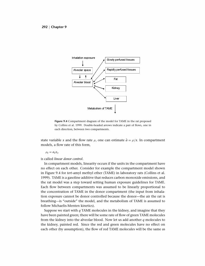
Figure 9.4 Compartment diagram of the model for TAME in the rat proposed
by Collins et al. 1999. Double-headed arrows indicate a pair of flows, one in
each direction, between two compartments.
state variable x and the flow rate ρ, one can estimate a = ρ/x. In compartment models, a flow rate of this form,
ρij = aijxj ,
is called linear donor control. In compartment models, linearity occurs if the units in the compartment have
no effect on each other. Consider for example the compartment model shown
in Figure 9.4 for tert-amyl methyl ether (TAME) in laboratory rats (Collins et al. 1999). TAME is a gasoline additive that reduces carbon monoxide emissions, and
the rat model was a step toward setting human exposure guidelines for TAME. Each flow between compartments was assumed to be linearly proportional to
the concentration of TAME in the donor compartment (the input from inhala-tion exposure cannot be donor controlled because the donor—the air the rat is
breathing—is “outside” the model, and the metabolism of TAME is assumed to
follow Michaelis-Menten kinetics). Suppose we start with q TAME molecules in the kidney, and imagine that they
have been painted green; there will be some rate of flow of green TAME molecules
from the kidney into the alveolar blood. Now let us add another q molecules to
the kidney, painted red. Since the red and green molecules have no effect on
each other (by assumption), the flow of red TAME molecules will be the same as

January 18, 2006 16:07 m26-main Sheet number 315 Page number 293
293 Building Dynamic Models
the flow of green ones. So doubling the number of molecules doubles the flow
rate. Thus, one cause of linearity in compartment models is dilution: the stuff being
tracked is so dilute that units never encounter each other. Conversely, if the units
in a compartment are common enough that they interact, linear donor control may not be appropriate. The mechanism leading to nonlinearity may be direct interactions among units, or it could be indirect, meaning that the units affect some system property that in turn influences the other units. For example,
• substrate molecules binding to receptor sites may decrease the chance of other
substrate molecules becoming bound
• when there are more prey available to a predator, each individual prey may be less
likely to get eaten because the other prey contribute to satiating the predators, or
because predators are busy hunting and consuming other prey
Exercise 9.5. Select one of the process rates from the model you proposed in Exercise
9.4 that could reasonably be modeled as linear, and explain why. Or, if there is no
such process in your model, select one rate and explain why a linear rate equation is
inappropriate.
9.3.2 Nonlinear Rates from “First Principles”
If enough is known about the mechanisms involved, that knowledge may imply
a particular nonlinear functional form for rate equations, though not necessarily
the numerical parameter values. For example,
• The law of mass action for chemical reactions states that reaction rates are
proportional to the product of the concentrations of the reactants.
• Newton’s laws of motion can be used to model animal locomotion as a set of rigid
links connected at joints. The constraints due to the links make the equations
nonlinear.
• Elasticity of heart tissue is coupled to its fluid motion in a nonlinear manner.
• The forces generated by muscle contraction depend nonlinearly on the length of
the muscle.
Nonlinear functional forms also arise as consequences of biological assump-tions about the system. In theoretical models rate equations are often derived as
logical consequences of the model’s biological hypotheses. For example,
• In the enzyme kinetics model in Chapter 1, the assumed underlying reaction
scheme, combined with the law of mass action and assumptions about the relative
time scales, implied the Michaelis-Menten form for the rate.

January 18, 2006 16:07 m26-main Sheet number 316 Page number 294
294 Chapter 9
• In Ross’s epidemic models the bilinear contact rate was derived as a consequence of
assumptions about the transmission process.
• Membrane current through a population of channels depends upon the membrane
potential and the open probability for individual channels in the population. The
open probabilities are observed to vary in a way that must be modeled. In the
Hodgkin-Huxley and Morris-Lecar models (Chapter 3), the open probability of each
channel is expressed by gating variables, each of which is also a dynamic variable.
Exercise 9.6. Find a recent paper in your area of biology where one of the rate equa-tions for a dynamic model was derived from first principles, or as a consequence of biological assumptions about the system, rather than on the basis of empirical data. State the assumptions or principles involved, and explain how those were used to
derive the rate equation. Had you been the modeler, would you have made the same
assumptions and used the same form of the rate equation?
9.3.3 Nonlinear Rates from Data: Fitting Parametric Models
In more practical models the rate equations are often estimated from data so
that they quantitatively describe the system of interest. Continuing with the
simplest case—a rate ρ depending on a single state variable x—estimating a
rate equation from data means fitting a curve to a scatterplot of measurements
{(xi, ρ(xi)), i = 1, 2, . . . , N}. Two issues are involved: choosing a functional form, and estimating parameter values. We need to discuss the second question first—
given a model, how do you estimate parameter values from data?—because the
choice of functional form often comes down to seeing how well each of them
can fit the data. The data plotted in Figure 9.5a are the reproduction rate (estimated by the egg-
to-adult ratio) in asexually reproducing rotifers Brachionus calyciflorus feeding on
algae Chlorella vulgaris in experimental microcosms. These data come from some
of the experiments reported by Fussmann et al. (2000). The variation in algal density results from the predator-prey limit cycles that occur in this system under
suitable experimental conditions. Based on prior results with related organisms, a reasonable starting point is the Michaelis-Menten functional form
Vx y = . [9.5]
K + x
We want to find the values of V and K that give the best approximation to the
data, according to some quantitative criterion. A common criterion is to mini-mize the sum of squared errors,
N ( ∑ Vxi )2
SSE = yi − . [9.6]K + xii=1

January 18, 2006 16:07 m26-main Sheet number 317 Page number 295
295 Building Dynamic Models
Figure 9.5 Fitting a parametric rate equation model. (a) The data and fitted curve (b) Residuals plotted
against the independent variable (c) Quantile-quantile plot comparing the distribution of residuals
to the Gaussian distribution assumed by the least-squares fitting criterion (d) Data and fitted curve
on square root scale (e) Residuals from model fitted on square root scale (f) Quantile-quantile plot
for square root scale residuals. The dashed curves in panels (c) and (f) are pointwise 95% confidence
bands; the large number of points outside the confidence bands in panel (c) show that the residuals
do not conform to a Gaussian distribution.
This is called least squares. Most statistics packages can do least squares fitting of nonlinear models such as this one; in a general programming language you can
write a function to compute the SSE as a function of V and K, and then use a
minimization algorithm to find the parameter values that minimize the SSE (the
computer lab materials on this book’s web page include examples of these). Either
way, we find estimated values V = 0.72, K = 0.95 producing the curve drawn in
Figure 9.5a.

January 18, 2006 16:07 m26-main Sheet number 318 Page number 296
296 Chapter 9
The least squares method can be justified as an example of maximum likelihood
parameter estimation: choosing the parameter values that maximize the proba-bility of observing (under the model being fitted) the data that you actually did
observe. Maximum likelihood is a “gold standard” approach in classical statistics. If we evaluate methods for estimating parameters based on the asymptotic rate
at which estimates converge to the truth as the amount of data goes up, under
some mild technical conditions it can be proved that no other method can have a
convergence rate strictly better than that of maximum likelihood. This does not mean that maximum likelihood is always optimal. Rather, it is like a Swiss Army
knife: if it can do the job (i.e., if you can compute and maximize your model’s
likelihood), you typically won’t gain much by finding and using the exact best tool for the job.
Maximum likelihood leads to least squares estimation if the “errors” (the devi-ations between the model equation and the response data yi) follow a Gaussian
distribution with zero mean and constant variance. It is then a standard result that minimizing the sum of squares, as a function of model parameters, is equiv-alent to maximizing the likelihood.
The errors are not observable, but we can estimate them by fitting the model Vxi/( ˆand plotting the residuals ei = yi − ˆ K + xi), where V , K are the parameters
estimated by least squares. Assumptions about the errors can now be checked
by examining the residuals. Formal statistical methods for doing this have been
developed, but it is often effective just to plot the residuals as a function of the
independent variable and look for signs of trouble. In our case we see some (Figure
9.5b): there are no obvious trends in the mean or variance but the distribution
is rather asymmetric. More formally, we can use a quantile-quantile (Q-Q) plot (available in most statistics packages, and computed here using R) to examine
whether the residuals conform to a Gaussian distribution (Figure 9.5c). A Q-Q
plot compares the relative values of the largest, second-largest, third-largest, etc., values in a data set, against the expected values of those quantities in a sample of the same size from the reference distribution. A perfect match between the data
and the reference distribution results in the Q-Q plot being a straight line, and
clearly here it isn’t. The model [9.5] seems to be good, but the residuals do not conform to the
assumed error distribution. What do we do now? The simplest option is to just live with it. With non-Gaussian errors, least squares is no longer optimal but the estimates are still statistically acceptable; the same is true if the errors are
Gaussian but their variance is nonconstant1 (Gallant 1987, Chapters 1 and 2). The next-simplest option is transformation: find a scale of measurement on
which the error distribution conforms to the assumptions of least squares. The
1Technically, least squares estimates are still approximately Gaussian distributed, and still converge to the true
values as sample size increases.

January 18, 2006 16:07 m26-main Sheet number 319 Page number 297
297 Building Dynamic Models
problem in Figure 9.5 is an asymmetric distribution with a long tail of large values. To pull in that tail we need a concave-down transformation such as log or square
root. After some trial and error, square root transformation seems to do the trick. That is, the modified fitting criterion is √ 2
N ∑ √ VxiSSE2 = yi − K + xi
, [9.7] i=1
which gives parameter estimates V = 0.70, ˆˆ K = 1.1. Finally, we look again at residuals to make sure that the transformation really has improved things, and the
right-hand panels in Figure 9.5 confirm that it has. Instead of trial and error it is
possible to estimate the power transformation that does the best job of producing
Gaussian errors with constant variance; the procedures are described by Seber and
Wild (1989, Chapter 2). For these data the result is β = 0.41, not far from the
trial-and-error result. If transformation fails, then improving on least squares is more complicated
and case specific, and may require either direct application of maximum likeli-hood or case-specific methods. A discussion of likelihood methods is not feasible
here; Hilborn and Mangel (1997) give a very readable introduction. Fitting nonlinear regression models by least squares or maximum likelihood is
best done with a statistics program or package (never with spreadsheet programs, whose statistical functions are unreliable). Parameter estimates will generally be
accompanied by a confidence interval—a range of possible parameter values that are credible, based on the data. By convention 95% confidence intervals are usu-ally reported, or else a “standard error” σ for each parameter such that a range
of ±2σ centered at the estimated value is approximately a 95% confidence inter-val for large sample sizes. As Bayarri and Berger (2004) review, there are several different philosophical schools in statistics about how to define and compute
confidence intervals, but all methods recommended for practical use have the
same practical interpretation: in repeated applications to real data, the reported
95% confidence intervals obtained by a method should contain the true param-eter value at least 95 times out of 100. Confidence intervals are useful when
comparing model output against data—they limit how far parameters can be
“adjusted” to get a good fit to data. They are also a good basis for setting ranges
of parameter values to explore for sensitivity analysis (Chapter 8).
Exercise 9.7. Download the data from Figure 9.5 from this book’s web site, and write
a script to find least-squares parameter estimates for V and K on the untransformed
scale (you should find that you duplicate the values above) and again using power transformation with β = 0.41. Do your parameter estimates for β = 0.41 indicate
that trial-and-error choice of β = 0.5 was close enough?

January 18, 2006 16:07 m26-main Sheet number 320 Page number 298
298 Chapter 9
Exercise 9.8. How does the choice of power transformation in the last exercise affect the 95% confidence intervals for the parameter estimates?
9.3.4 Nonlinear Rates from Data: Selecting a Parametric Model
We can now return to the task of selecting a functional form. The first step is to
plot your data. If the data appear to be nonlinear, a useful next step is to see if some transformation straightens them out. For example, allometric relationships
by = ax [9.8]
are pervasive in biology (see, e.g., Niklas 1994; West et al. 1997). Taking loga-rithms of both sides we have
log y = log a + b log x, [9.9]
a linear relationship between log-transformed variables. The Michaelis-Menten
relationship [9.5] is linearized by taking the inverses of both sides: ( K
)1 1 1 = + . [9.10]y V x V
The reason for trying this approach is that the eye is pretty good at telling if data
are linear, but much poorer at telling the difference between one nonlinear curve
and another.2
The next fallback is to “round up the usual suspects,” a roster of conventional forms that modelers have used repeatedly to approximate nonlinear functional relationships. Figure 9.6 shows some of the most widely used forms. Replacing
y by y − y0 where y0 is a constant produces a vertical shift of the curve by y0; replacing x by x − x0 produces a horizontal shift by amount x0. Finally, if all else fails one can fall back on parametric families that allow you to add more
and more parameters until the curve looks like your data. The most familiar are
polynomials, y = a0 + a1x + a2x2 + · · · . The use of conventional functional forms is widespread, but we urge you to use
them only as a last resort. The only thing special about them is their popularity. So before resorting to a conventional form, it is worthwhile thinking again if your knowledge of the underlying process, or reasonable assumptions about it, might suggest a rate equation with some mechanistic meaning. Or, if you have
sufficient data, it might be preferable to use instead a nonparametric rate equation
(as discussed below).
2Finding a linearizing transformation makes it tempting to fit the model by linear regression on the transformed
scale. However, the transformation that produces linearity might not also produce errors that satisfy the assumptions
for least-squares fitting. Fitting [9.5] by linear regression of 1/y on 1/x is often cited as an example of poor statistical practice. Small values of y and x transform into large values of their inverses, which are typically very inaccurate due
to measurement errors even if the errors are small. When you fit on the transformed scale, the parameter estimates
can be severely distorted in an attempt to fit those inaccurate values.

January 18, 2006 16:07 m26-main Sheet number 321 Page number 299
299 Building Dynamic Models
Figure 9.6 Some widely used equations forms to fit nonlin-
ear functional relationships.
It is often difficult to identify one clearly best form for a rate equation just by visually comparing how well they fit the data (e.g., repeating something like
Figure 9.5 for each candidate). Quantitative comparison can be based on values
of the fitting criterion [e.g., [9.6] or [9.7]]. To fairly compare equations with
different numbers of fitted parameters, those with more parameters need to be
January 18, 2006 16:07 m26-main Sheet number 322 Page number 300
300 Chapter 9
penalized—otherwise a cubic polynomial will always be better than a quadratic
and worse than a quartic. Various criteria of this sort have been proposed, which
attempt to pick the level of complexity that optimizes the ability to predict future
observations. Two widely used criteria for least squares fitting are
AIC = N log(SSE/N) + 2p, BIC = N log(SSE/N) + p log N,
where N is the number of data points, and p is the number of parameters in
the model.3 The model with the smallest value of AIC or BIC is preferred. For
N/p < 40 a more accurate version of AIC is recommended, AICc = AIC + 2p(p +
1)/(N − p − 1) (Burnham and Anderson 2002). If AIC and BIC disagree, they at least provide a range of plausible choices.
An alternative to approximate criteria such as AIC or BIC is to estimate directly
the predictive accuracy of different functional forms, using a computational ap-proach called cross validation (CV). For each data point (xi, yi), you
1. Form a reduced data set consisting of all other data points.
θ [−i]2. Fit the model to the reduced data set, obtaining estimated parameter vector ˆ .
θ [−i]3. Generate a prediction of yi using the reduced data set, yi = f (xi , ).
4. Having done the above for all i, you compute the cross-validated prediction error
C = ∑
iN =1(yi − yi )
2.
That is, you use the data in hand to simulate the process of fitting the model, predicting future data, and seeing how well you did. Repeating this process for
each possible functional form lets you determine which of them gives the best predictive power.
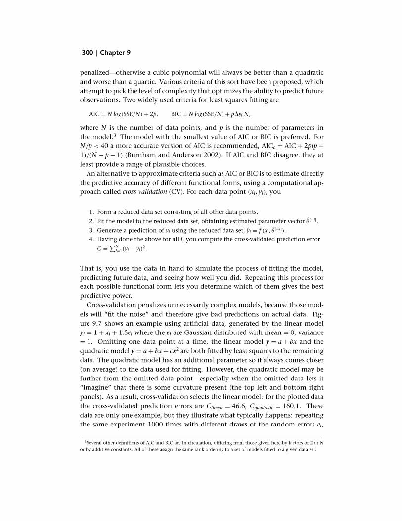
Cross-validation penalizes unnecessarily complex models, because those mod-els will “fit the noise” and therefore give bad predictions on actual data. Fig-ure 9.7 shows an example using artificial data, generated by the linear model yi = 1 + xi + 1.5ei where the ei are Gaussian distributed with mean = 0, variance
= 1. Omitting one data point at a time, the linear model y = a + bx and the
quadratic model y = a + bx + cx2 are both fitted by least squares to the remaining
data. The quadratic model has an additional parameter so it always comes closer
(on average) to the data used for fitting. However, the quadratic model may be
further from the omitted data point—especially when the omitted data lets it “imagine” that there is some curvature present (the top left and bottom right panels). As a result, cross-validation selects the linear model: for the plotted data
the cross-validated prediction errors are Clinear = 46.6, Cquadratic = 160.1. These
data are only one example, but they illustrate what typically happens: repeating
the same experiment 1000 times with different draws of the random errors ei,
3Several other definitions of AIC and BIC are in circulation, differing from those given here by factors of 2 or N
or by additive constants. All of these assign the same rank ordering to a set of models fitted to a given data set.

January 18, 2006 16:07 m26-main Sheet number 323 Page number 301
301 Building Dynamic Models
Figure 9.7 Cross validation for linear versus quadratic regression. In each panel, one of the 6 data
points (shown as an open circle) is omitted from the data set, and the two models are fitted to the
other data points. The solid line is the fitted linear model, the dashed line is the fitted quadratic.
the linear model was selected 78% of the time, which is pretty good for six noisy
data points. Cross-validation is also not the last word in computer-intensive
model selection; more sophisticated methods with better accuracy are available
and development in this area is active (Efron 2004). It is important to remember that cross-validation aims to find the rate equation
that predicts best, given the data available. This is not the same as finding the
“right” model, because of the tradeoff between model error and parameter error. If data are limited or noisy, any criterion based on prediction accuracy should
select a model that is simpler than the truth. This distinction is often overlooked,

January 18, 2006 16:07 m26-main Sheet number 324 Page number 302
302 Chapter 9
and a model selected on the basis of prediction error is incorrectly claimed to
represent the true structure of the underlying biological system. Finally, rather than trying to identify a unique best model one can use an
average over plausible models, weighting each one based on how well it fits the
data (Burnham and Anderson 2002). Model averaging is still not widely used, so
its effectiveness in dynamic modeling remains to be seen. We personally favor
the methods discussed in the next section, which are more flexible and eliminate
the issue of selecting a functional form.
9.4 Nonlinear Rates from Data: Nonparametric Models
If the tools just described for nonlinear rate equations seem like a random bag of tricks, that is not quite true. They are a bag of tricks developed when slow and
expensive computers first made it possible to consider simple nonlinear models, instead of the linear models that had previously been the only possibility. Fast cheap computing opens up a new possibility that allows nonlinear rate models to
be more realistic and less subjective: nonparametric curve fitting. In this context nonparametric means that instead of an explicit formula like [9.5], there is a recipe
for computing the y value (process rate) for any given value of a state variable or
exogenous variable x, based on the data. So instead of choosing from a limited
menu like Figure 9.6, the curve can take whatever shape the data require. The simplest nonparametric recipe (simple enough not to require a computer)
is connect the dots: draw straight lines between successive data points. Figure 9.8a
shows an example, using data from Hairston et al. (1996). The data are the frac-tion of egg clutches laid by the freshwater copepod Diaptomus sanguineus that hatch immediately rather than remaining dormant, as a function of the date on
which the clutch was produced. The first and last dates plotted are field data. The intermediate dates are lab experiments, done in growth chambers set to
mimic natural conditions on those dates (water temperature and photoperiod). Because only a few growth chambers were available, there are data for only a
few dates, but each data point is reliable because a lot of copepods fit happily
into one growth chamber—sample sizes are roughly 100–200. Because we trust each data point but know nothing about what happens in between them, “con-nect the dots” is reasonable. A more sophisticated version is to run a smooth
curve through the data points, such as a spline. A spline is a polynomial on each
interval between data points, with coefficients chosen so that polynomials for
adjacent intervals join together smoothly. In this instance there was a “first prin-ciples” model based on population genetics theory (the light curve drawn in the
figure), and connect-the-dots does a good job of approximating the theoretically
derived function.

January 18, 2006 16:07 m26-main Sheet number 325 Page number 303
303 Building Dynamic Models
Figure 9.8 Examples of nonparametric rate equations based on data. (a) Two
versions of “connect the dots.” Heavy solid curve is linear interpolation,
dashed curve is cubic spline interpolation. The light solid curve is a parametric
model derived from population genetics theory for traits controlled by many
genetic loci. (b) The solid curve is a nonparametric regression spline, fitted
subject to the constraints of passing through (0, 0) and being monotonically
non-decreasing. For comparison, the dashed curve is the Michaelis-Menten
model fitted to the same data ( V = 0.7, K = 1.1).
The curves in Figure 9.8a go exactly through each data point—this is called in-terpolation. Interpolation no longer makes sense in a situation like Figure 9.5—a
large number of imprecise data points. Nonparametric methods for this situa-tion only became possible with sufficient computing power, so we are still in the
stage where many different approaches are under parallel development, with new
ideas appearing each year. We are partial to regression splines (Ruppert et al. 2003; Wood 2003) because they make it relatively easy to impose biologically mean-

January 18, 2006 16:07 m26-main Sheet number 326 Page number 304
304 Chapter 9
ingful qualitative constraints. Figure 9.8b shows an example (solid curve), with
two constraints imposed: y = 0 for x = 0 (no feeding implies no breeding), and
increased food supply leads to increased (or at least not decreased) reproduction
rate. The use of nonparametric curves as one component of a complex statistical model is well established in statistics (Bickel et al. 1994), but applications to dy-namic modeling have only recently begun; see Banks and Murphy (1989), Wood
(1994, 1999, 2001), Ellner et al. (1998, 2002) for some applications. Another im-portant use of nonparametric models is the one illustrated in Figure 9.8b: a close
correspondence between nonparametric and parametric models supports use of that parametric model, since it indicates that there is no additional structure in
the data that the parametric model cannot capture.
9.4.1 Multivariate Rate Equations
The curse of dimensionality (Chapter 1) afflicts even dynamic models if a rate
equation depends on several variables. Half a dozen values can reveal the shape
of a curve in one variable (Figure 9.8a), but would say little about a function of two variables and even less about a function of three. When data are sparse, some
kind of simplification is needed. The ideal situation is to know the right functional form. If you have a pre-
determined three-parameter equation, it doesn’t matter how many variables 2are involved—fitting ρ = ax + by + cz2 is no harder than fitting ρ = a + bx + cx ,
given the same number of data points. The functional form may come from first principles, or experience that a particular form has worked for the same process
in models of related systems. Alternatively, first principles or past experience may justify assumptions about
the functional form. The two most widely used are the following.
1. Multiplication of rate limiting factors:
ρ(x1, x2, . . . , xm) = ρ0ρ1 (x1)ρ2(x2) · · · ρm (xm). [9.11]
The assumption is that the relative effect of each variable xi is independent of the
other variables, analogous to a beam of light passing through a series of filters,
each of which blocked a fixed fraction of the incoming photons. So for example, if
a plant depends on N and P for growth, a given decrease in N availability causes
the same percentage loss in growth rate, regardless of how much P is available. In
statistics this would be called a generalized additive model (GAM) for f = log ρ,
f (x1, x2, . . . , xm) = f0 + f1 (x1) + f2(x2 ) + · · · + fm (xm).
In R the MGCV package can be used to fit GAMs in which each fj is a
nonparametric regression spline.

January 18, 2006 16:07 m26-main Sheet number 327 Page number 305
305 Building Dynamic Models
x1 2 3 4 5 6 1 1 1 1 1
x2 2 2 2 2 2 1 2 3 4 5
ρ 10.0 10.7 9.6 8.3 5.4 16.6 8.3 4.2 3.6 6.2
Table 9.1 Artificial “data” for Exercise 9.9
2. Liebig’s Law of the Minimum:
ρ(x1, x2, . . . , xm) = ρ0 × min{ρ1(x1), ρ2(x2 ), . . . , ρm(xm)}. [9.12]
Here we imagine a chain of subprocesses that are necessary for the overall process
to occur, and the slowest of these acts as the rate-limiting step. Under this model,
if a plant depends on N and P for growth and there is a severe N shortage, growth
will be limited by lack of N and the (relatively) abundant P will not cause any
additional decrease.
The advantage of these is that the multivariate model is reduced to a series of univariate models, each of which can be estimated using far less data. In addition, the individual functions can be based totally separate data sets, each involving
variation in only one of the factors affecting the rate, and combined to model a situation where several factors are varying at once. The disadvantage of using
these conventional forms is that you are skating on thin ice unless there are good
reasons to believe that the chosen form is correct—such as results on similar
systems, or evidence to support the mechanistic assumptions that lead to the
particular form. Adopting a conventional assumption based on precedent should
always be a last resort. Finally, there are purely statistical approaches to dimension reduction, such as
the generalized linear, neural network, and projection pursuit regression models
(see, e.g., Venables and Ripley 2002). However, these have no clear biological interpretation, so choosing one of these over another is difficult unless data are
so plentiful that dimension reduction is not necessary.
Exercise 9.9. For the “data” in Table 9.1, consider whether one of the models listed
above is adequate.
(a) Which data points would you use to estimate ρ1? Which would you use for ρ2? Write
a script to fit curves to these data (hint: the obvious works), and plot the data and
estimated function curves.
(b) Combine your estimated ρ1 and ρ2 into an overall model, and evaluate how well it does
by plotting observed versus predicted values.
Exercise 9.10. Propose a simple model for competition between two bacterial strains
grown on an otherwise sterile “broth” of finely pulped vegetable (imagine cucumber

January 18, 2006 16:07 m26-main Sheet number 328 Page number 306
306 Chapter 9
in a blender on “high” for 10 minutes, diluted with water). The model is a step in
identifying strains of bacteria that can be used to inoculate food products, so that if they are exposed to high temperatures and start to spoil, toxic bacteria will be
outcompeted by harmless species. The salient biological facts are as follows: • The experimental setup is closed culture (no inflow or outflow), kept well mixed at
constant conditions.
• Substrate (the resources the bacteria need to survive, grow, reproduce ) is available and
not limiting.
• The main difference between strains is in their response to, and production rate of,
lactic acid which they release into the culture medium. Lactic acid is a mildly toxic
by-product of the metabolic processes that lead to growth and reproduction; as it
accumulates the species have a decrease in their growth rates. On the time scale of
interest, lactic acid does not degrade.
Your final set of equations can include parameters that would need to be estimated, and functions for process rates that would need to be determined experimentally.
9.5 Stochastic Models
Stochasticity can enter models in too many ways for us to consider or even enu-merate here. But trying to do so would be pointless, because no fundamentally
new issues arise. The only addition is the task of estimating the parameters that characterize the probability distributions for random components in the dynamic
equations. To illustrate this point, we consider some types of stochastic models
that we have seen in previous chapters.
9.5.1 Individual-Level Stochasticity
Models at the level of individual agents—for example, individual ion channels
flipping between closed and open, or individual-based ecological models—are
defined by the probabilities of different events rather than by process rates. Given
the state of the system or of an individual agent, the model proceeds by asking
what events could happen next, and what are their probabilities of occurring?
For example, if a plant’s size is x:
1. What is the probability that it will still be alive next year?
2. Live or die, how many seeds will it produce between now and next year, and how
many of those will still be alive at the next census?
3. If it lives, how big will it be?
Questions of these types are the basis for any agent-based model. The agent’s state
is determined by a list of state variables—some discrete (alive or dead, healthy or

January 18, 2006 16:07 m26-main Sheet number 329 Page number 307
( )
307 Building Dynamic Models
infected, 0 or 1 for each bit in a Tierran organism, etc.), and some continuous. The model lists rules for how these change over time, and possibly for how they
affect the numbers of agents that are created or destroyed. Typically the rules
are stochastic, so the answer to “how big will it be?” is a probability distribu-tion rather than a single number, with numerical values obtained from random
number generators. When the response variable is discrete—for example, live or die—the model re-
quires a function p(x) giving the probability of living as a function of agent state
x. We can associate the outcomes with numerical scores 1 = live and 0 = die, but least squares fitting is still not appropriate because the distribution of outcomes
is discrete and highly non-Gaussian. Fortunately the appropriate methods are so
widely used that the basic models are included in most statistics packages. For
binary choice (two possible outcomes) the most popular approach is a transfor-mation method called logistic regression,
log p = f (x1, x2, . . . , xm). [9.13]
1 − p
Here p is the probability of one of the possible outcomes, and (x1, x2, . . . , xm) are
the variables in the model that might affect the probability. Most statistics pack-ages can at least do linear or polynomial logistic regression, and many allow f to
be a nonparametric function. Much less is available prepackaged for more than
two possible outcomes; most statistics packages can only fit logistic regression
models in which the f for each outcome is linear. However, the likelihood func-tion for more general logistic regression models is relatively simple, so these can
be fitted via maximum likelihood. In situations with multiple outcomes—such as offspring numbers in the list
above—it is often more natural to use a parametric probability distribution to
specify the outcome probabilities. For example, individual-based population
models often assume that the number of offspring in a litter follows a Poisson dis-tribution, whose mean depends on variables characterizing the individual (size, age, etc.) This is called Poisson regression and at least the linear model is available
in many statistics packages. However it is again relatively easy to write down the
likelihood function for other parametric probability distributions, for example, to modify the Poisson so that a litter must contain at least one offspring.
So fitting probability functions for an individual-level stochastic model is con-ceptually no different from fitting rate functions in a differential equation model, and the issues of model selection and complexity remain the same: linear or non-linear? which nonlinear form? what form of multivariate response? and so on.
For continuous variables—such as individual size in the list above—the most common approach is a parametric probability distribution with parameters de-pending on agent and system state variables. This is like fitting a parametric
process rate equation, except that functions are fitted for all parameters of the
distribution, not just the mean. Figure 9.9 is an example, the size the following

January 18, 2006 16:07 m26-main Sheet number 330 Page number 308
308 Chapter 9
0 2 4 6 8
02
46
8
Log size t
Log
size
t+1
0 2 4 6 8
−1.
5−
0.5
0.5
1.5
Log size t
Sca
led
resi
dual
s
Scaled residuals
Fre
quen
cy
−2 −1 0 1 2
020
4060
8010
0
−3 −2 −1 0 1 2 3
−1.
5−
0.5
0.5
1.5
Normal quantiles
Obs
erve
d qu
antil
es
Figure 9.9 Fitting and testing a parametric model for the distribution of individual size in surviving
plants of Onopordum illyricum (from Rees et al. 1999; data provided by Mark Rees). Panels (clockwise
from top left) show the data from one study site with fitted mean and variance functions, the scaled
residuals versus original size, Normal quantile-quantile plot and histogram of scaled residuals.
year of surviving plants in Illyrian thistle, Onopordum illyricum (Rees et al. 1999).The average log-transformed new size is a linear function of log-transformed cur-rent size, but the scatter about the regression line is not constant. Rees et al.(1999) proposed exponental size-dependence in growth variance. Letting x andy denote the current and next-year log transformed sizes, the fitted model for oneof their study sites is a Gaussian distribution of y with mean and variance
y(x) ≡ E(y|x) = 3.3 + 0.55x, σ 2y (x) ≡ Var(y|x) = 32.2e−0.58y(x). [9.14]
Linear models such as [9.14] with nonconstant variance can be estimated bygeneralized least squares in many statistics packages.

January 18, 2006 16:07 m26-main Sheet number 331 Page number 309
∏
Building Dynamic Models 309
The dashed lines in the scatterplot of the data (Figure 9.9) are curves based on
the fitted variance function that should include 90% of all data. Clearly there are
some problems: roughly 1% of the 720 plants in the data set had atypically poor
growth, and these “outliers” have to be considered separately or ignored. Drop-ping the outliers, we can check the variance model in [9.14] by examining the
scaled residuals ri = (yi − y(xi))/σy (xi). If the model is valid then their variance
should be independent of xi, which appears to be true, and their distribution
should be approximately Gaussian.4 The histogram and quantile-quantile plot for the scaled residuals indicate that the Gaussian assumption is not too bad (re-call that exactly Gaussian scaled residuals would would give a perfectly straight quantile-quantile plot), but it is probably the least satisfactory aspect of this in-dividual growth model.
There are also nonparametric estimates of probability distributions that can
be used instead of a parametric distribution family (Venables and Ripley 2002, Chapter 5). For use in an agent-based simulation the simplest is to draw a scaled
residual r at random from those computed from the data, and let the new size of a size-x individual be y(x) + σy (x)r.
Exercise 9.11. The Poisson probability distribution with mean λ is given by p(k) ≡
Pr (X = k) = e−λλk /k!. The likelihood of obtaining a sample of values x1, x2, · · · , xn is
n
L = p(xi ). i=1
(a) To see what the Poisson distribution is like, write a script file that generates 6 samples of
size 50 from the Poisson distribution with mean 3, and produces a plot with a histogram
of each sample. Then modify your script to do the same for samples of size 250 from
the Poisson distribution with mean 20.
(b) Write a script file that computes − log (L) as a function of λ for the following data,
and use it to find the maximum likelihood estimate of λ. Data values are x =
1, 1, 1, 1, 2, 2, 2, 2, 2, 3, 4, 4, 4, 4, 5.
9.5.2 Parameter Drift and Exogenous Shocks
“Parameter drift” means that the dynamics at any given moment follow a de-terministic set of dynamic equations, but the parameters in the rate equations
change randomly over time. The ideal situation is if the parameters themselves
can be observed and measured. Then from multiple observations of the parame-ters, one can fit a probability distribution to their pattern of variation over time.
4More accurate residual scalings are possible and are recommended with small samples; see Davison and Hinkley
1997, section 6.2.

January 18, 2006 16:07 m26-main Sheet number 332 Page number 310
√
310 Chapter 9
The situation is more difficult when the observable quantities are process rates
that are jointly determined by state variables and parameter values. Then if the
rate equation involves more than one parameter, the value of the process rate
does not uniquely determine the parameter values that produced it. The most common way of dealing with this problem is to assume it out of existence, by
adding a single parameter to represent the net effect of all stochastic variation in
model parameters (and anything else), and then assuming that all other param-eters are constant. That is, instead of a rate equation like
V (t )x ρ(x, t ) =
K(t ) + x
with stochastic variation in the parameters V and K, the rate equation might be
Vx ρ(x, t) =
K + x + e(t) (additive noise)
[9.15]
ρ(x, t) = Vx
K + x (1 + e(t )) (multiplicative noise).
The terms with fixed parameter values are intepreted as the average process rate, and e(t) produces random deviations from the average rate. In these equations, the randomness takes the form of external “shocks” to the system, rather than
really specifying the mechanistic basis for fluctuations in process rates. The payoff is that fitting such models can be relatively straightforward. Consider for example
Figure 9.5. We previously developed a model of the form
√ Vxρ(x) = + e [9.16]
K + x
where the random “errors” e have a Gaussian distribution with 0 mean and con-stant variance. Ignoring the scatter about the fitted curve, we get a deterministic
rate equation. But to take that variability into account in the model, the only
additional task is to estimate their variance. As before, the residuals from the fit (Figure 9.5e) provide an estimate of the errors, and it is straightforward to show
that for Gaussian-distributed errors, the maximum likelihood estimate of the er-ror variance, σe
2, is given by the mean of the squared residuals. For these data we .have σe = 0.18 so the resulting stochastic rate model is √ 2
Vx ρ(x, t ) = + 0.18z(t ) [9.17]
K + x
where the z(t) are Gaussian random variables with mean 0, variance 1. In fitting the model this way, we have assumed that the measured values of the
rate are accurate—that the scatter about the fitted curve represents real variation
in the rate, rather than errors in measurements. Otherwise, the fitted model overestimates the real variability in the rates. If there is measurement error, and if the measurement error variance is known, the model can be corrected to account

January 18, 2006 16:07 m26-main Sheet number 333 Page number 311
∑ (
311 Building Dynamic Models
for the component of the residual variance that is due to measurement errors. For example, if the measurement errors have constant known variance σ 2
me , we
subtract this from the estimate of the total variance and have the estimate σ 2 = e
SSE2/N − σ 2 me .
9.6 Fitting Rate Equations by Calibration
So far we have assumed that data are available at the process level—simultaneous
measurements of the process rate and of the state and exogenous variables
thought to affect its value. When such data are not available, it may still be possi-ble to fit the model by adjusting parameters so that model output—state variable
trajectories—comes as close as possible in some sense to experimental measure-ments of state variable dynamics. This is called calibration. In some applications, the purpose of the model is to estimate otherwise unknowable parameters by cal-ibration, such as the viral turnover rate in HIV (Chapter 6). Calibrating a model is then a way to connect the unobservable process rates and observable macro-scopic quantities at the level of state variables, so that obtainable data can be
used to estimate quantities that cannot be measured directly. For example, consider fitting the so-called θ -logistic population model
dx/dt = rx(1 − (x/K)θ )
to a set of data on population growth over time (Figure 9.10). Although the
model is a differential equation, we can still estimate parameters by least squares: find the values of r, K, θ and the initial value x0, that minimize
N
SSE = x(t) − x(t ) )2 , [9.18]
t =0
where x(t) are the data values, and x(t) are solutions of the model. The starting
value is treated as a parameter: were we to start model solutions at the first value
in the data set, we would be giving that data point special treatment by insisting
that the model match it exactly. Estimating parameters by minimizing SSE, or
similar measures of the difference between model trajectories and data is called
path calibration or trajectory matching. In principle, path calibration of a deterministic model is just an example of
nonlinear least squares, no different from nonlinear least squares fitting of [9.5], and it is commonly used for fitting dynamic models to data. Path calibration
can also be used to estimate models with some nonparametric components (e.g., Banks and Murphy 1989; Banks et al. 1991; Wood 1994, 2001).
Path calibration does not make sense for stochastic models: two runs of the
model yield different values of SSE, as would two replications of the experiment on the real system. Instead, we can fit the model by making model simulations

January 18, 2006 16:07 m26-main Sheet number 334 Page number 312
312 Chapter 9
2 4 6 8
0 10
0 20
0 30
0 40
0 50
0
Pop
ulat
ion
coun
t
10 12 14
time(d)
Figure 9.10 Results from calibration of the θ -logistic population model to data
on population growth of Paramecium aurelia feeding on bacteria in Cerophyl
growth medium; the data were digitized from Figure 2b in Veilleux (1976).
resemble the data in terms of statistical properties such as the mean, variance, and autocorrelation of state variable trajectories. Statisticians call this moment calibration or method of moments. It is widely used in economic modeling, be-cause deliberate experiments are impossible and models have to be estimated
and evaluated based on their predictions about observable variables such as stock
prices, exchange rates, energy demand, etc. In the economics literature there is
well-developed theory and numerous applications of moment calibration (e.g., Gourièroux and Montfort 1996), and biological applications are starting to appear
(Ellner et al. 1995, 2002; Kendall et al. 1999; Turchin and Ellner 2000). However, ad hoc moment calibration is widespread, for instance, roughly estimating a few
parameters by adjusting them until the model gives the right mean, variance, or range of state variables. More recently, general simulation-based methods are
being developed for calibrating stochastic models by maximum likelihood or re-lated Bayesian procedures, which can allow for both measurement errors in the
data and inherently stochastic dynamics (e.g., Gelman et al. 2003; Calder et al. 2003; de Valpine 2004). This is a rapidly developing area, which will increase
in importance as the necessary tools are incorporated into user-friendly statistics
packages.
Exercise 9.12. The data plotted in Figure 9.10 are tabulated in Table 9.2. Are they
fitted as well by the conventional logistic model in which θ = 1? To answer this
question, write scripts to do the following:

January 18, 2006 16:07 m26-main Sheet number 335 Page number 313
313 Building Dynamic Models
t 1 2 3 4 5 6 7 8 9 10 11 12 13 14 x(t) 15.58 30.04 66.05 141.6 274.6 410 468.8 526.4 472.5 496.6 489.5 492 496.8 473
Table 9.2 Experimental data on growth of Paramecium aurelia that are plotted in Figure 9.10, digitized
from Figure 2b in Veilleux (1976)
Run Period (days) Nmax/Nmin
1 38.5 ± 1.5 36 ± 17
2 34.0 ± 1.5 77 ± 26
3 35.1 ± 0.4 240 ± 160
Table 9.3 Summary statistics for estimating the parameters
P and δ of model (9.20) by moment calibration
(a) Path-calibrate by least squares the full model including θ and the reduced model with
θ = 1, and find which model would be selected by the AIC and BIC. Remember that the
initial condition x0 is included in the parameter count when fitting by path calibration.
(b) Path-calibrate both models repeatedly to reduced data sets that each omit one data
point, and find which model would be selected by the cross-validation criterion.
Exercise 9.13. This exercise is based on Chapter 8 of Nisbet and Gurney (1982). The
following simple model was proposed for oscillations in laboratory populations of sheep blowfly:
dN/dt = PN(t − τ )e−N(t−τ )/N0 − δN(t) [9.19]
N(t) is the number of sexually mature adults, and τ is the time required for a newly
laid egg to develop into a sexually mature adult, about 14.8 days. Setting x = N/N0
the model becomes
dx/dt = Px(t − τ )e−x(t−τ ) − δx(t). [9.20]
Write a script to estimate the values of P and δ by moment calibration, i.e., choosing
their values to match as well as possible the estimates in Table 9.3 of the period of population oscillations, and the ratio between population densities at the peak and
trough of the cycles. As conditions varied between experimental runs, parameters
should be estimated separately for each of the three runs. Independent data suggest δ ≈ 0.3/d and 100 < Pτ < 220 for the first two experiments.
Note: your script can solve the model by representing it as a big density-dependent matrix model. Divide individuals into m + 1 age classes 0 − h, h −
2h, 2h − 3h, . . . , (m − 1)h − τ , and “older than 1” (adults) where h = τ/m. One iter-ation of the matrix model then corresponds to h units of time. The number of births in
a time step is n0(t + 1) = hPnm+1(t )e−nm+1 (t), individuals younger than 1 have 100%

January 18, 2006 16:07 m26-main Sheet number 336 Page number 314
314 Chapter 9
survival (pj = 1 for j = 0, 1, 2, . . . , m − 1), and adults have survival e−δh . This method
is computationally inefficient but makes it easy to add finite-population effects, for example, if the number of births in a time interval is a random variable with mean
given by the expression above.
Exercise 9.14. Derive completely one of the process rate equations for the model from Exercise 9.4. That is, for one of the processes in the model, derive the equation
which gives the rate as a function of the state variables and/or exogenous variables
which affect it. This includes both the choice of functional form, and estimating
numerical values for all parameters in the equation. (As noted above “rate” could
also be an outcome probability or probability distribution of outcomes, depending
on the kind of model.)
(a) Describe the process whose rate equation you are deriving.
(b) Explain the rationale for your choice of functional form for the equation. This could
involve data; the hypothesis being modeled; previous experience of other modelers;
etc.
(c) Estimate the parameters, explaining what you are doing and the nature and source
of any data that you are using. If the available data do not permit an exact estimate,
identify a range of plausible values that could be explored when running the model.
(d) Graph the “final product”: the relationship between the process rate and one or two
of the state or exogenous variables influencing it, in the rate equation.
9.7 Three Commandments for Modelers
The principles of model development can be summarized as three important rules:
1. Lie
2. Cheat 3. Steal
These require some elaboration. Lie. A good model includes incorrect assumptions. Practical models have to
be simple enough that the number of parameters does not outstrip the available
data. Theoretical models have to be simple enough that you can figure out what they’re doing and why. The real world, unfortunately, lacks these properties. So
in order to be useful, a model must ignore some known biological details, and
replace these with simpler assumptions that are literally false.

January 18, 2006 16:07 m26-main Sheet number 337 Page number 315
315 Building Dynamic Models
Cheat. More precisely, do things with data that would make a statistician ner-vous, such as using univariate data to fit a multivariate rate equation by multipli-cation of limiting factors or Liebig’s law of the minimum, and choosing between
those options based on your biological knowledge or intuition. Statisticians like
to let data “speak for themselves.” Modelers should do that when it is possible, but more often the data are only one input into decisions about model structure, the rest coming from the experience and subject-area knowledge of the scientists
and modelers. Steal. Take ideas from other modelers and models, regardless of discipline.
Cutting-edge original science is often done with conventional kinds of models
using conventional functional forms for rate equations—for example, compart-ment models abound in the study of HIV/AIDS. If somebody else has developed
a sensible-looking model for a process that appears in your model, try it. If some-body else invested time and effort to estimate a parameter in a reasonable way, use it. Of course you need to be critical, and don’t hesitate to throw out what you’ve stolen if it doesn’t fit what you know about your system.
9.8 Evaluating a Model
Everybody knows what it means to evaluate a model: you plot model output and
your data on the same graph, as in Figure 9.10, and if the points are near the line, the model is good. But there is more to it than that. Following Caswell (1976), we consider an extreme example to explain why.
Figure 9.11 shows a model where the points are quite near the line: a remark-ably simple model for growth of the global human population developed by Von
Foerster et al. (1960). Von Foerster et al. (1960) argued that the dominant force in
human population expansion was our ability to cooperate in advancing our stan-dard of living, thus increasing lifespan and offspring survival. Consequently, the
net (birth-death) rate r should be modeled as an increasing function of population
size N. They proposed the model r = aN1/K , a, K > 0; hence dN/dt = aN1+1/K .
This model can be solved explicitly—the form of the solution is
N(t ) = α(τ − t)−K . [9.21]
Equation [9.21] fits the historical data remarkably well: it says that log N(t) should
be a linear function of log(τ − t), and for the data and solution in Figure 9.11 this
linear regression explains over 97% of the variance in log N(t). So we have a good model, right? But look at what happens in [9.21] as t → τ :
N(t) becomes infinite. Von Foerster et al. (1961) called this Doomsday and esti-mated it to occur on Friday November 13, 2026: “Our great-great grandchildren
will not starve to death, they will be squeezed to death” (von Foertster et al. 1960, p. 1295). With an additional forty years of data, the estimate of Dooms-
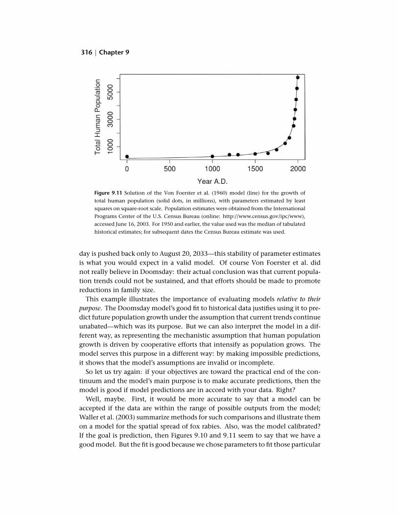
January 18, 2006 16:07 m26-main Sheet number 338 Page number 316
316 Chapter 9
Figure 9.11 Solution of the Von Foerster et al. (1960) model (line) for the growth of
total human population (solid dots, in millions), with parameters estimated by least
squares on square-root scale. Population estimates were obtained from the International
Programs Center of the U.S. Census Bureau (online: http://www.census.gov/ipc/www),
accessed June 16, 2003. For 1950 and earlier, the value used was the median of tabulated
historical estimates; for subsequent dates the Census Bureau estimate was used.
day is pushed back only to August 20, 2033—this stability of parameter estimates
is what you would expect in a valid model. Of course Von Foerster et al. did
not really believe in Doomsday: their actual conclusion was that current popula-tion trends could not be sustained, and that efforts should be made to promote
reductions in family size. This example illustrates the importance of evaluating models relative to their
purpose. The Doomsday model’s good fit to historical data justifies using it to pre-dict future population growth under the assumption that current trends continue
unabated—which was its purpose. But we can also interpret the model in a dif-ferent way, as representing the mechanistic assumption that human population
growth is driven by cooperative efforts that intensify as population grows. The
model serves this purpose in a different way: by making impossible predictions, it shows that the model’s assumptions are invalid or incomplete.
So let us try again: if your objectives are toward the practical end of the con-tinuum and the model’s main purpose is to make accurate predictions, then the
model is good if model predictions are in accord with your data. Right?
Well, maybe. First, it would be more accurate to say that a model can be
accepted if the data are within the range of possible outputs from the model; Waller et al. (2003) summarize methods for such comparisons and illustrate them
on a model for the spatial spread of fox rabies. Also, was the model calibrated?
If the goal is prediction, then Figures 9.10 and 9.11 seem to say that we have a
good model. But the fit is good because we chose parameters to fit those particular

January 18, 2006 16:07 m26-main Sheet number 339 Page number 317
317 Building Dynamic Models
data, so it does not say whether the same model could fit a second experiment, or whether another model might fit even better. If all available data were used
to calibrate the model, then none is “left over” to test the model. Unless data
are so plentiful that one can fit the model to part of the data and test it on the
remainder (and be honest about it), successful calibration is only weak support for a model.
One more try: if your model lies toward the practical end of the continuum
and its main purpose is to make accurate predictions, then the model is bad if model output is inconsistent with the data. Right?
Well, maybe. It could also mean that some of your parameters are poorly
estimated, so it would be worth seeing if you can calibrate the model to fit the
data. If not, you probably do have a bad model for purposes of prediction. If the
model can be calibrated, you are back in the previous quandary that the model fits because you fiddled with parameters to make it fit.
In short: evaluating a model is hard. Fortunately it is easier, and usually more
useful, to evaluate several models. The difficulties elaborated (and exaggerated) above stem from trying to benchmark a model against reality. No model can pass
that test perfectly, so you’re left trying to decide how close is “close enough”. In
contrast, when we compare how well two different models can account for the
data, both are measured on the same scale.
9.8.1 Comparing Models
The appropriate criteria for comparing models are determined (as always) by your
goals, so there is no “one size fits all” approach, or even an exhaustive list of possibilities.
At one extreme, if the only concern is prediction accuracy, then the methods
for individual rate equations discussed in Section 9.3.4 apply equally to the model as a whole. In particular, one always has recourse to cross-validation, in principle. At the level of the entire model, it is often not feasible to automate the process
of omitting individual data points and rebuilding the model. Instead, the data
can be divided into several subsets, and subsets are omitted rather than single
data points. Subsets can be chosen at random or in some systematic way. For
example, if the models are fitted by calibrating to state variable trajectories, you
might first calibrate to the first half of the data and see how well each model predicts the second half, then calibrate to the second half and try to predict the
first. Different approaches are needed if you are concerned with mechanistic validity.
In some situations a structured cross-validation may be useful. For example, again
assuming that you have data on several state variables, you might omit in turn the
entire data series for one of the state variables, calibrate the model to the others, and see how well the model predicts the omitted state variable. A model that

January 18, 2006 16:07 m26-main Sheet number 340 Page number 318
318 Chapter 9
properly captures the causal relations among state variables would be expected
to do better in such a test than one that has the wrong “wiring diagram.”
More formal statistical approaches are possible if the models are nested, mean-ing that one of them (the reduced model MR) can be obtained by removing com-ponents of the other (the full model MF ), or by constraining parameters of the full model to particular values. Comparison of these models addresses the scientific
question of whether the additional features of the full model are actually playing
a role in the system dynamics. Because MF necessarily has more parameters (all those in MR and then some), it always can fit the data better than MR. So in
order to assay the actual relevance of the additional processes in MF , we have
to determine whether the improvement in fit is too large to be solely a result of the additional parameters. We do this by adopting the null hypothesis that MR is true, and computing the probability (under this assumption) of getting an
improvement in fit as large, or larger, than the one that actually occurred. If this sounds familiar, it is: this is a standard statistical hypothesis test. However, in contrast to most descriptive statistical models, for dynamic models we typ-ically have to use simulation methods to implement the test—a process called
(somewhat confusingly) parametric bootstrap. In principle the recipe is simple:
1. Fit MR and MF to the data, and record for each a quantitative measure of how well
they fit the data.
2. Use simulations of MR to generate artificial data sets that mimic the real one (in
terms of the amount, type, and accuracy of the data).
3. Fit MR and MF to each artificial data set, and record for each the same quantitative
measure of how well they fit the data.
4. Compare the observed improvement (step 1) to those occurring in artifical data
where MR is really true. If the observed improvement is atypically large relative to
those on the artificial data (e.g., larger than all but 5% or 1%), this implies that the
improved fit of MF is not just due it having additional parameters, hence the
additional structure in MF captures some features actually present in the data.
Note that a negative result is harder to interpret—as is true in general for statistical hypothesis tests. If the reduced model is not rejected, it may mean that the
added ingredients in the full model are not present in the real system, or it may
mean that the data set was too small or too inaccurate to demonstrate that those
ingredients are present. Pascual et al. (2000) used parametric bootstrap to test the hypothesis that
cholera outbreaks are linked to climate variability associated with the El Niño
Southern Oscillation (ENSO), mediated by increased sea-surface temperatures and
higher numbers of zooplankton bearing the bacterium causing cholera. The data
were monthly estimates of cholera incidence from a hospital in Bangladesh from
1980–1999, where a sample of incoming patients were tested for cholera. The

January 18, 2006 16:07 m26-main Sheet number 341 Page number 319
319 Building Dynamic Models
reduced model included local seasonal climate variation as an exogenous vari-able affecting cholera dynamics; the full model added an index of ENSO based
on sea-surface temperatures in the Pacific. The full and reduced models were
compared based on their ability to predict cholera incidence two months into
the future. One thousand artificial data sets were generated from the reduced
model by adding randomly shuffled residuals to the reduced model’s predictions
of monthly cholera incidence. Fitting both models to these artificial data, the
improvements in fit were all smaller than on the real data, providing very strong
evidence of a link between ENSO and cholera. Similarly, Turchin et al. (2003) used parametric bootstrap to compare models for
population outbreaks of larch budmoth in Swiss forests. Budmoth outbreaks oc-cur at regular intervals of 8–9 years, with roughly 100,000-fold variation between
abundances at the peak and trough of the cycles. For the last several decades the
experimental research has focused on the generally-accepted hypothesis that the
cycles are driven by the interactions between budmoth and their food supply, larch needles. Turchin et al. (2003) also considered effects of parasitoids attack-ing the budmoth. Parametric bootstrap was used to compare models with and
without the effects of parasitoids, and the results were decisive: the improvement in fit on the real data was larger than all but 0.3% of the improvements on the
artificial data, demonstrating that the accepted hypothesis for the cycles was in-correct. A second reduced model with parasitoids but no effect of food supply
was also rejected, hence it appears that both parasitoids and food supply affect budmoth dynamics.
As these examples illustrate, comparative evaluation of models is no different from comparative evaluation of two scientific hypotheses based on their ability
to account for all the available evidence. It suffers from the same limitations—
for example, there is broad scope for fiddling with hypotheses to explain away
discrepancies, in the same way that there is broad scope for adjusting model parameters to fit whatever data are available. However, models add the potential for
• generating and testing predictions based on complex hypotheses involving the
interactions of many components and processes, and
• making quantitative predictions, so that discrimination among hypotheses can be
based on quantitative comparisons of how well each model can account for the
available data.
That is, models used as quantitative expressions of contending hypotheses extend
the scope of the scientific method. They let us evaluate ideas about an entire
system, rather than about its individual parts one by one, and let us make those
evaluations as rigorous as our knowledge and data allow.

January 18, 2006 16:07 m26-main Sheet number 342 Page number 320
320 Chapter 9
Exercise 9.15. Produce two alternative versions of your model from Exercise 9.4, differing in some biologically meaningful assumption. Do an appropriate comparative
evaluation to determine which model corresponds best with the actual behavior of the study system.
9.9 References
Banks, H. T., and K. A. Murphy. 1989. Estimation of nonlinearities in parabolic models for growth, predation, and dispersal of populations. Journal of Mathematical Analysis and Applications 141: 580–602.
Banks, H. T., L. W. Botsford, F. Kappel, and C. Wang. 1991. Estimation of growth and survival in size-structured cohort data—an application to larval striped bass (Morone saxatilis). Journal of Mathematical Biology 30: 125–150.
Bayarri, M. J., and J. O. Berger. 2004. The interplay of Bayesian and frequentist analysis. Statistical Science 19: 58–80.
Bickel, P. J, C.A.J. Klassen, Y. Ritov, and J. A. Wellner. 1993. Efficient and Adaptive Estimation for Semiparametric Models. Johns Hopkins University Press, Baltimore, MD.
Bolker, B. M., S. W. Pacala, and W. J. Parton, Jr. 1998. Linear analysis of soil decomposition: insights from the Century model. Ecological Applications 8: 425–439.
Burnham, K. P., and D. R. Anderson. 2002. Model Selection and Multi-Model Inference. Springer, New York.
Calder, C., M. Lavine, P. Muller, and J. S. Clark. 2003. Incorporating multiple sources of stochasticity into dynamic population models. Ecology 84: 1395–1402.
Caswell, H. 1976. The validation problem. Pages 313–325 in B. C. Patten (ed.), Systems Analysis and Simulation in Ecology. Academic Press, New York, Vol. 4.
Collins, A. S., S.C.J. Sumner, S. J. Borghoff, and M. A. Medinsky. 1999. A physiological model for tert-amyl methyl ether and tert-amyl alcohol: hypothesis testing of model structures. Toxicological Sciences 49: 15–28.
Colwell, R. 1996. Global climate and infectious disease: The cholera paradigm. Science 274: 2025– 2031.
Cox, P., R. Betts, C. Jones, S. Spall, and I. Totterdell. 2000. Acceleration of global warming due to carbon-cycle feedbacks in a coupled climate model. Nature 408, 184–187.
Cox, P. 2001. Description of the “TRIFFID” Dynamic Global Vegetation Model. Hadley Centre Tech-nical Note 24. Available at http://www.met-office.gov.uk/research/hadleycentre/pubs
Cramp, D. G., and E. R. Carson. 1979. Dynamics of blood glucose and its regulating hormones. In D. A. Linkens (ed.), Biological Systems, Modeling and Control. IEE, London.
Davison, A. C., and D. V. Hinkley. 1997. Bootstrap Methods and Their Application. Cambridge Univer-sity Press, Cambridge, U.K.
de Valpine, P. 2004. Monte Carlo state-space likelihoods by weighted posterior kernel density esti-mation. Journal of the American Statistical Association 99: 523–536.
Efron, B. 2004. The estimation of prediction error: Covariance penalties and cross-validation. Journal of the American Statistical Association 99: 619–632.
Ellner, S., A. R. Gallant, and J. Theiler. 1995. Detecting nonlinearity and chaos in epidemic data. Pages 229–247 in D. Mollison (ed.), Epidemic Models: Their Structure and Relation to Data. Cambridge University Press, Cambridge, U.K.
Ellner, S. P., B. A. Bailey, G. V. Bobashev, A. R. Gallant, B. T. Grenfell, and D. W. Nychka. 1998. Noise and nonlinearity in measles epidemics: combining mechanistic and statistical approaches to population modeling. American Naturalist 151: 425–440.
Ellner, S. P., Y. Seifu, and Robert H. Smith. 2002. Fitting population models to time series data by gradient matching. Ecology 83: 2256–2270.
Fussman, G., S. P. Elner, K. W. Shertzer, and N. G. Hairston, Jr. 2000. Crossing the Hopf bifurcation in a live predator-prey system. Science 290: 1358–1360.

January 18, 2006 16:07 m26-main Sheet number 343 Page number 321
321 Building Dynamic Models
Gallant, A. R. 1987. Nonlinear Statistical Models. Wiley, New York. Gelman, A., D. B. Rubin, J. B. Carlin, and H. S. Stern. 2003. Bayesian Data Analysis, 2nd edition.
Chapman & Hall/CRC Press, Boca Raton, FL. Gourièroux, C., and A. Montfort. 1996. Simulation-based Econometric Inference. Oxford University
Press, Oxford, U.K. Hairston, N. G., Jr., C. M. Kearns, and S. Ellner. 1996. Phenotypic variation in a zooplankton egg
bank. Ecology 77: 2382–2392. Hett, J. M., and R. J. O’Neill. 1974. Systems analysis of the Aleut ecosystem. Artic Anthropology 11:
31–40. Hilborn, R., and M. Mangel. 1997. The Ecological Detective: Confronting Models with Data. Princeton
University Press, Princeton, NJ. Kendall, B. E., C. J. Briggs, W. W. Murdoch, P. Turchin, S. P. Ellner, E. McCauley, R. Nisbet, and S.
N. Wood. 1999. Why do populations cycle? A synthesis of statistical and mechanistic modeling approaches. Ecology 80: 1789–1805.
Ludwig, D., and C. J. Walters. 1985. Are age-structured models appropriate for catch-effort data? Canadian Journal of Fisheries and Aquatic Science 42: 1066–1072.
Niklas, K. J. 1994. Plant Allometry: the Scaling of Form and Process. University of Chicago Press, Chicago. Nisbet, R. M., and W.S.C. Gurney. 1982. Modelling Fluctuating Populations. Wiley, New York. NREL (Natural Resource Ecology Laboratory). 2001. Century soil organic matter model version 5,
user’s guide and reference. Natural Resource Ecology Laboratory, Colorado State University, Fort Collins, CO. Online at http://www.nrel.colostate.edu/projects/century5
Parton, W., D. Schimel, C. Cole, and D. Ojima. 1987. Analysis of factors controlling soil organic levels of grasslands in the Great Plains. Soil Science Society of America Journal 51: 1173–1179.
Parton, W., J. Stewart, and C. Cole. 1988. Dynamics of C, N, P and S in grassland soils: A model. Biogeochemistry 5: 109–131.
Pascual, M., X. Rodo, S. P. Ellner, R. Colwell, and M. J. Bouma. 2000. Cholera dynamics and the El Niñ-Southern Oscillation. Science 289: 1766–1769.
Rees, M., A. Sheppard, D. briese, and M. Mangel. 1999. Evolution of size-dependent flowering in Onopordum illyricum: A quantitative assessment of the role of stochastic selection pressures. American Naturalist 154: 628–651.
Ruppert, D., M. P. Wand, and R. U. Carroll. 2003. Semiparametric Regression. Cambridge University Press, New York.
Seber, G.A.F., and C. J. Wild. 1989. Nonlinear Regression. Wiley, New York. Turchin, P., and S. P. Ellner. 2000. Living on the edge of chaos: Population dynamics of Fennoscan-
dian voles. Ecology 81: 3099–3116. Turchin, P., S. N. Wood, S. P. Ellner, B. E. Kendall, W. W. Murdoch, A. Fischlin, J. Casas, E. McCauley,
and C. J. Briggs. 2003. Dynamical effects of plant quality and parasitism on population cycles of larch budmoth. Ecology 84: 1207–1214.
Venables, W. N., and B. D. Ripley. 2002. Modern Applied Statistics with S, 4th edition. Springer, New York.
Veilleux, B. G. (1976). The analysis of a predatory interaction between Didinium and Paramecium. MS Thesis, University of Alberta.
Von Foerster, H., L. W. Amiot, and P. M. Mora. 1960. Doomsday: Friday, 13 November, A.D. 2026. Science 132: 1291–1295.
Waller, L. A., D. Smith, J. E. Childs, and L. A. Real. 2003. Monte Carlo assessments of goodness-of-fit for ecological simulation models. Ecological Modelling 164: 49–63.
West, G. B., J. H. Brown, and B. J. Enquist. 1997. A general model for the origin of allometric scaling laws in biology. Science 276: 122–126.
Wood, S. N. 1994. Obtaining birth and death rate patterns from structured population trajectories. Ecological Monographs 64: 23–44.
Wood, S. N. 1999. Semi-parametric population models. Aspects of Applied Biology 53: 41–50. Wood, S. N. 2001. Partially specified ecological models. Ecological Monographs 71: 1–25. Wood, S. N. 2003. Thin-plate regression splines. Journal of the Royal Statistical Society, Series B 65:
95–114.