Embed Size (px)
Citation preview
Review for the Final Exam
Stephen A. Edwards
Columbia University
Fall 2017

Table of Contents IThe Final Exam
Structure of a Compiler
ScanningLanguages and Regular ExpressionsNFAsTranslating REs into NFAsBuilding a DFA from an NFA: Subset Construction
ParsingResolving AmbiguityRightmost and Reverse-Rightmost DerivationsBuilding the LR(0) AutomatonBuilding an SLR Parsing TableShift/Reduce Parsing
Table of Contents II
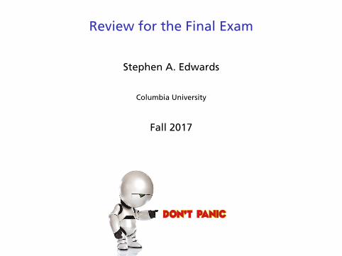
Types and Static SemanticsScopeApplicative vs. Normal-Order Evaluation
Runtime EnvironmentsStorage Classes and Memory LayoutThe Stack and Activation RecordsIn-Memory Layout IssuesThe HeapAutomatic Garbage CollectionObjects and InheritanceExceptions
Table of Contents III
Code GenerationIntermediate RepresentationsOptimization and Basic Blocks
The Lambda CalculusLambda ExpressionsBeta-reductionAlpha-conversionReduction OrderNormal FormThe Y Combinator
Table of Contents IV
Logic Programming in PrologProlog ExecutionThe Prolog EnvironmentUnificationThe Searching AlgorithmProlog as an Imperative Language
The Final
75 minutes
Closed book
One double-sided sheet of notes of your own devising
Comprehensive: Anything discussed in class is fair game,including things from before the midterm
Little, if any, programming
Details of O’Caml/C/C++/Java/Prolog syntax not required
Broad knowledge of languages discussed
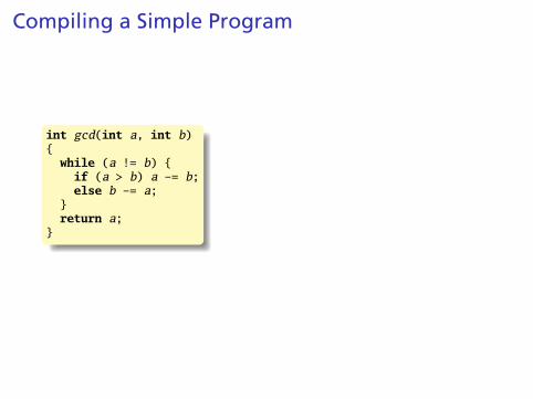
Compiling a Simple Program
int gcd(int a, int b){while (a != b) {if (a > b) a -= b;else b -= a;
}return a;
}

What the Compiler Seesint gcd(int a, int b){while (a != b) {if (a > b) a -= b;else b -= a;
}return a;
}
i n t sp g c d ( i n t sp a , sp in t sp b ) nl { nl sp sp w h i l e sp( a sp ! = sp b ) sp { nl sp sp sp sp if sp ( a sp > sp b ) sp a sp - = sp b; nl sp sp sp sp e l s e sp b sp - = spa ; nl sp sp } nl sp sp r e t u r n spa ; nl } nl
Text file is a sequence of characters
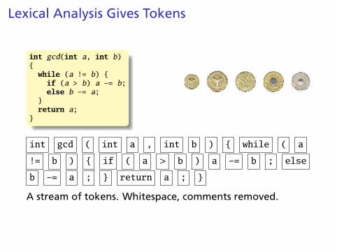
Lexical Analysis Gives Tokens
int gcd(int a, int b){while (a != b) {if (a > b) a -= b;else b -= a;
}return a;
}
int gcd ( int a , int b ) { while ( a
!= b ) { if ( a > b ) a -= b ; else
b -= a ; } return a ; }
A stream of tokens. Whitespace, comments removed.
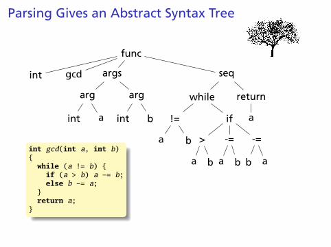
Parsing Gives an Abstract Syntax Tree
func
int gcd args
arg
int a
arg
int b
seq
while
!=
a b
if
>
a b
-=
a b
-=
b a
return
a
int gcd(int a, int b){while (a != b) {if (a > b) a -= b;else b -= a;
}return a;
}
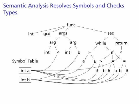
Semantic Analysis Resolves Symbols and ChecksTypes
Symbol Table
int a
int b
func
int gcd args
arg
int a
arg
int b
seq
while
!=
a b
if
>
a b
-=
a b
-=
b a
return
a
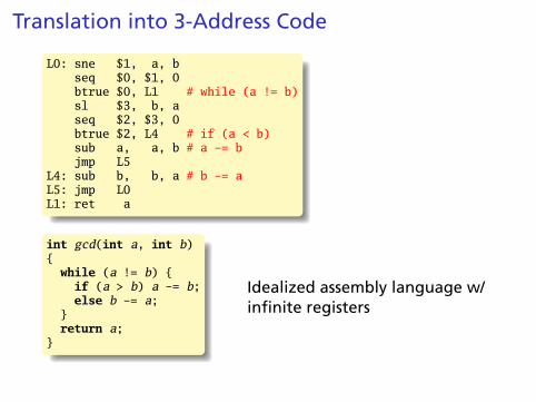
Translation into 3-Address Code
L0: sne $1, a, bseq $0, $1, 0btrue $0, L1 # while (a != b)sl $3, b, aseq $2, $3, 0btrue $2, L4 # if (a < b)sub a, a, b # a -= bjmp L5
L4: sub b, b, a # b -= aL5: jmp L0L1: ret a
int gcd(int a, int b){while (a != b) {if (a > b) a -= b;else b -= a;
}return a;
}
Idealized assembly language w/infinite registers
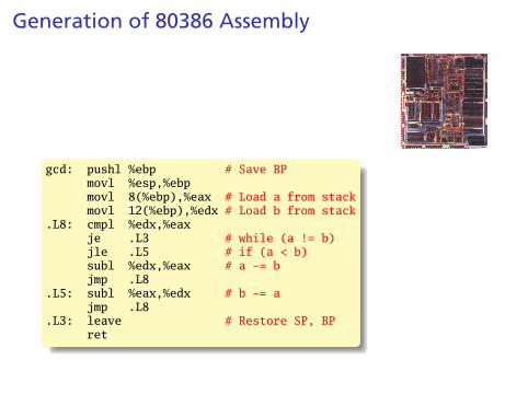
Generation of 80386 Assembly
gcd: pushl %ebp # Save BPmovl %esp,%ebpmovl 8(%ebp),%eax # Load a from stackmovl 12(%ebp),%edx # Load b from stack
.L8: cmpl %edx,%eaxje .L3 # while (a != b)jle .L5 # if (a < b)subl %edx,%eax # a -= bjmp .L8
.L5: subl %eax,%edx # b -= ajmp .L8
.L3: leave # Restore SP, BPret
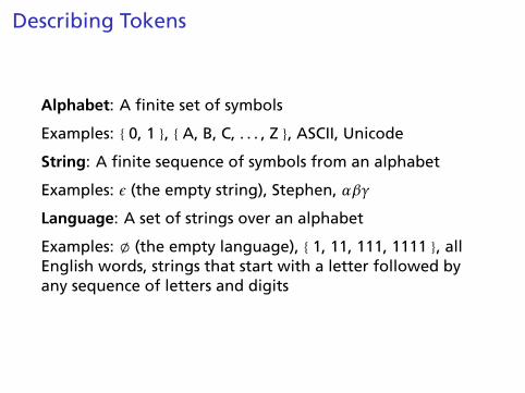
Describing Tokens
Alphabet: A finite set of symbols
Examples: { 0, 1 }, { A, B, C, . . . , Z }, ASCII, Unicode
String: A finite sequence of symbols from an alphabet
Examples: ε (the empty string), Stephen, αβγ
Language: A set of strings over an alphabet
Examples: ; (the empty language), { 1, 11, 111, 1111 }, allEnglish words, strings that start with a letter followed byany sequence of letters and digits
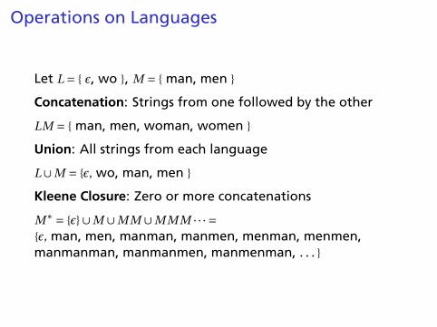
Operations on Languages
Let L = { ε, wo }, M = { man, men }
Concatenation: Strings from one followed by the other
LM = { man, men, woman, women }
Union: All strings from each language
L∪M = {ε, wo, man, men }
Kleene Closure: Zero or more concatenations
M∗ = {ε}∪M ∪M M ∪M M M · · · ={ε, man, men, manman, manmen, menman, menmen,manmanman, manmanmen, manmenman, . . . }
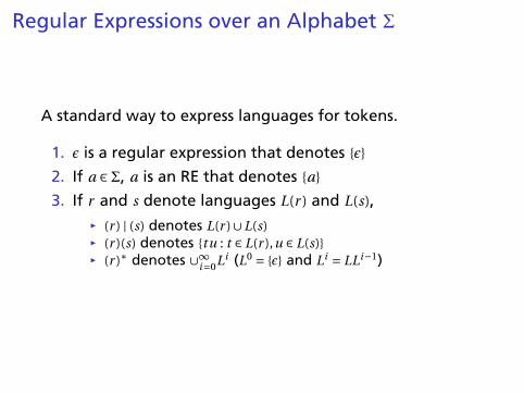
Regular Expressions over an Alphabet Σ
A standard way to express languages for tokens.
1. ε is a regular expression that denotes {ε}
2. If a ∈Σ, a is an RE that denotes {a}
3. If r and s denote languages L(r ) and L(s),Ï (r ) | (s) denotes L(r )∪L(s)Ï (r )(s) denotes {tu : t ∈ L(r ),u ∈ L(s)}Ï (r )∗ denotes ∪∞
i=0Li (L0 = {ε} and Li = LLi−1)
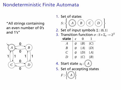
Nondeterministic Finite Automata
“All strings containingan even number of 0’sand 1’s”
A B
C D
0
011
0
01 1
1. Set of states
S :
{A B C D
}2. Set of input symbols Σ : {0,1}3. Transition function σ : S×Σε → 2S
state ε 0 1A ; {B} {C }B ; {A} {D}C ; {D} {A}D ; {C } {B}
4. Start state s0 : A
5. Set of accepting states
F :
{A
}
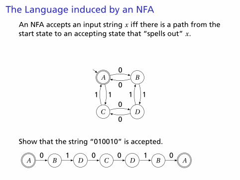
The Language induced by an NFA
An NFA accepts an input string x iff there is a path from thestart state to an accepting state that “spells out” x.
A B
C D
0
011
0
01 1
Show that the string “010010” is accepted.
A B D C D B A0 1 0 0 1 0
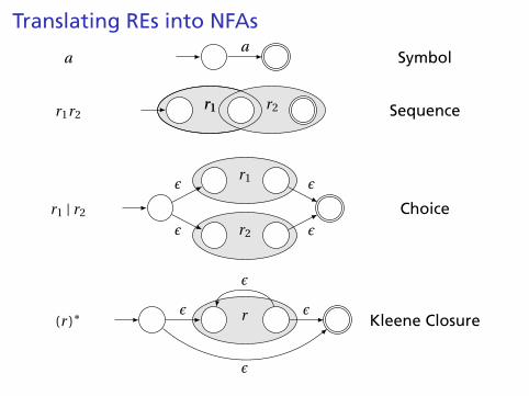
Translating REs into NFAs
aa
Symbol
r1r2r1 r2r1 Sequence
r1 | r2
r1
r2
ε
ε
ε
ε
Choice
(r )∗ rε ε
ε
ε
Kleene Closure
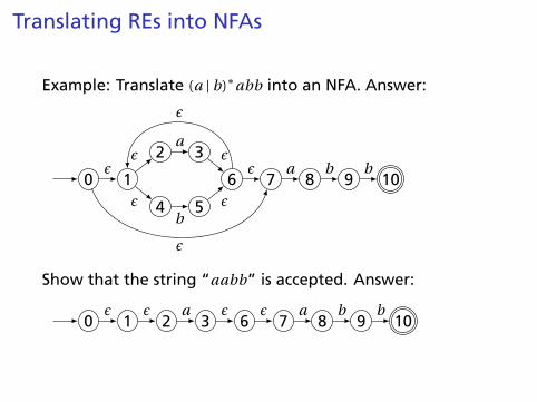
Translating REs into NFAs
Example: Translate (a | b)∗abb into an NFA. Answer:
0 1
2 3
4 5
6 7 8 9 10ε
εa
εb
ε
ε
ε a b b
ε
ε
Show that the string “aabb” is accepted. Answer:
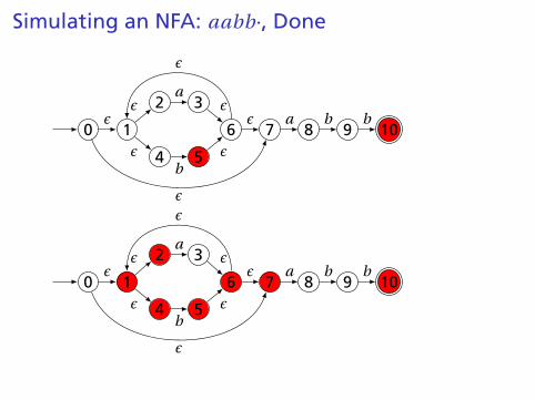
0 1 2 3 6 7 8 9 10ε ε a ε ε a b b
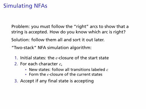
Simulating NFAs
Problem: you must follow the “right” arcs to show that astring is accepted. How do you know which arc is right?
Solution: follow them all and sort it out later.
“Two-stack” NFA simulation algorithm:
1. Initial states: the ε-closure of the start state2. For each character c,
Ï New states: follow all transitions labeled cÏ Form the ε-closure of the current states
3. Accept if any final state is accepting
Simulating an NFA: ·aabb, Start
0 1
2 3
4 5
6 7 8 9 10ε
εa
εb
ε
ε
ε a b b
ε
ε
0 1
2 3
4 5
6 7 8 9 10ε
εa
εb
ε
ε
ε a b b
ε
ε

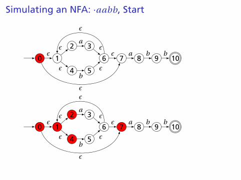
Simulating an NFA: a·abb
0 1
2 3
4 5
6 7 8 9 10ε
εa
εb
ε
ε
ε a b b
ε
ε
0 1
2 3
4 5
6 7 8 9 10ε
εa
εb
ε
ε
ε a b b
ε
ε
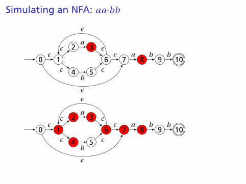
Simulating an NFA: aa·bb
0 1
2 3
4 5
6 7 8 9 10ε
εa
εb
ε
ε
ε a b b
ε
ε
0 1
2 3
4 5
6 7 8 9 10ε
εa
εb
ε
ε
ε a b b
ε
ε
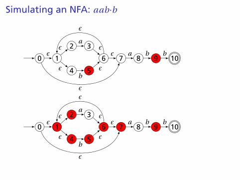
Simulating an NFA: aab·b
0 1
2 3
4 5
6 7 8 9 10ε
εa
εb
ε
ε
ε a b b
ε
ε
0 1
2 3
4 5
6 7 8 9 10ε
εa
εb
ε
ε
ε a b b
ε
ε
Simulating an NFA: aabb·, Done
0 1
2 3
4 5
6 7 8 9 10ε
εa
εb
ε
ε
ε a b b
ε
ε
0 1
2 3
4 5
6 7 8 9 10ε
εa
εb
ε
ε
ε a b b
ε
ε
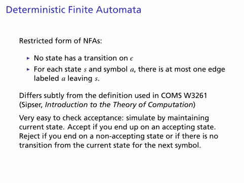
Deterministic Finite Automata
Restricted form of NFAs:
Ï No state has a transition on ε
Ï For each state s and symbol a, there is at most one edgelabeled a leaving s.
Differs subtly from the definition used in COMS W3261(Sipser, Introduction to the Theory of Computation)
Very easy to check acceptance: simulate by maintainingcurrent state. Accept if you end up on an accepting state.Reject if you end on a non-accepting state or if there is notransition from the current state for the next symbol.
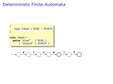
Deterministic Finite Automata
{type token = ELSE | ELSEIF
}
rule token =parse "else" { ELSE }
| "elseif" { ELSEIF }
e l s e i f
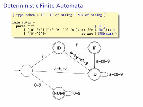
Deterministic Finite Automata
{ type token = IF | ID of string | NUM of string }
rule token =parse "if" { IF }
| [’a’-’z’] [’a’-’z’ ’0’-’9’]* as lit { ID(lit) }| [’0’-’9’]+ as num { NUM(num) }
NUM
ID IF
ID
0–9
i
a–hj–z
f
a–z0–9
a–eg–z0–9
0–9
a–z0–9
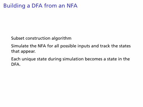
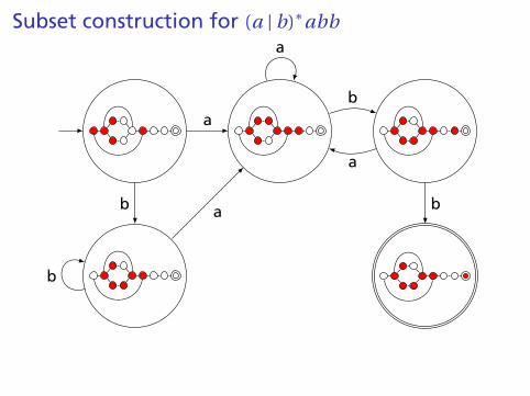
Building a DFA from an NFA
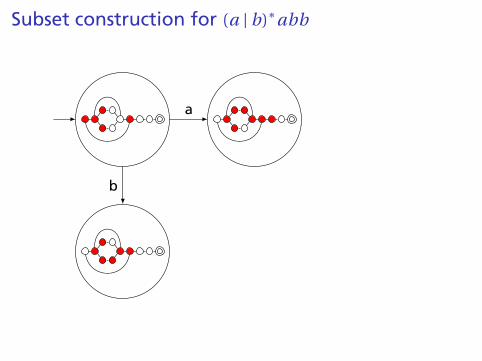
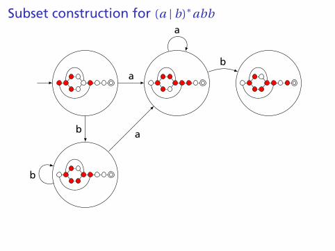
Subset construction algorithm
Simulate the NFA for all possible inputs and track the statesthat appear.
Each unique state during simulation becomes a state in theDFA.
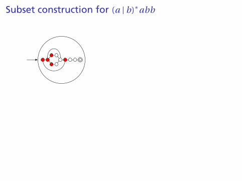
Subset construction for (a | b)∗abb
a
b
a
b
b
a
a
ba
b
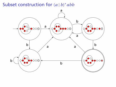
Subset construction for (a | b)∗abb
a
b
a
b
b
a
a
ba
b
Subset construction for (a | b)∗abb
a
b
a
b
b
a
a
ba
b
Subset construction for (a | b)∗abb
a
b
a
b
b
a
a
b
a
b
Subset construction for (a | b)∗abb
a
b
a
b
b
a
a
ba
b
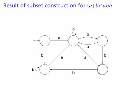
Result of subset construction for (a | b)∗abb
a
b
ab
b
a
a
ba
b
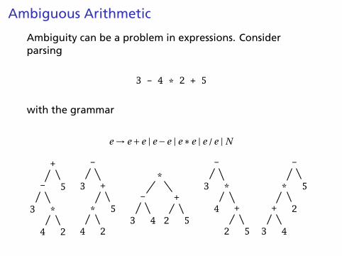
Ambiguous Arithmetic
Ambiguity can be a problem in expressions. Considerparsing
3 - 4 * 2 + 5
with the grammar
e → e +e | e −e | e ∗e | e /e | N
+
-
3 *
4 2
5
-
3 +
*
4 2
5
*
-
3 4
+
2 5
-
3 *
4 +
2 5
-
*
+
3 4
2
5
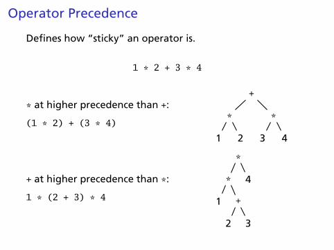
Operator Precedence
Defines how “sticky” an operator is.
1 * 2 + 3 * 4
* at higher precedence than +:
(1 * 2) + (3 * 4)
+
*
1 2
*
3 4
+ at higher precedence than *:
1 * (2 + 3) * 4
*
*
1 +
2 3
4
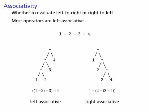
AssociativityWhether to evaluate left-to-right or right-to-left
Most operators are left-associative
1 - 2 - 3 - 4
-
-
-
1 2
3
4
-
1 -
2 -
3 4
((1−2)−3)−4 1− (2− (3−4))
left associative right associative
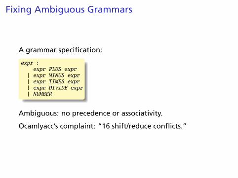
Fixing Ambiguous Grammars
A grammar specification:
expr :expr PLUS expr
| expr MINUS expr| expr TIMES expr| expr DIVIDE expr| NUMBER
Ambiguous: no precedence or associativity.
Ocamlyacc’s complaint: “16 shift/reduce conflicts.”
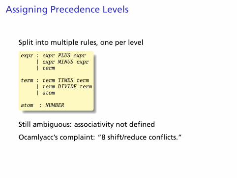
Assigning Precedence Levels
Split into multiple rules, one per level
expr : expr PLUS expr| expr MINUS expr| term
term : term TIMES term| term DIVIDE term| atom
atom : NUMBER
Still ambiguous: associativity not defined
Ocamlyacc’s complaint: “8 shift/reduce conflicts.”
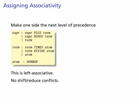
Assigning Associativity
Make one side the next level of precedence
expr : expr PLUS term| expr MINUS term| term
term : term TIMES atom| term DIVIDE atom| atom
atom : NUMBER
This is left-associative.
No shift/reduce conflicts.
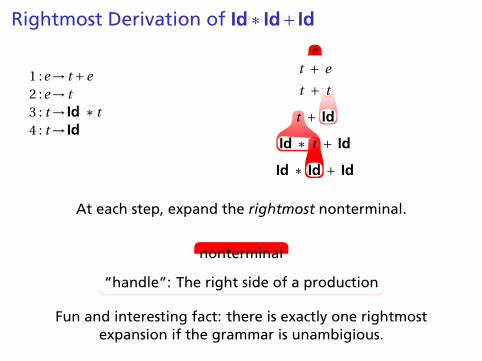
Rightmost Derivation of Id∗ Id+ Id
1 :e→ t +e2 :e→ t3 : t → Id ∗ t4 : t → Id
et + e
t + t
t + Id
Id ∗ t + Id
Id ∗ Id + Id
At each step, expand the rightmost nonterminal.
nonterminal
“handle”: The right side of a production
Fun and interesting fact: there is exactly one rightmostexpansion if the grammar is unambigious.
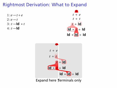
Rightmost Derivation: What to Expand
1 :e→ t +e2 :e→ t3 : t → Id ∗ t4 : t → Id
et + et + t
t + Id
Id ∗ t + Id
Id ∗ Id + Id
Expand here ↑Terminals only
e
t + e
t + t
t + Id
Id ∗ t + Id
Id ∗ Id + Id
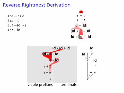
Reverse Rightmost Derivation
1 :e→ t +e2 :e→ t3 : t → Id ∗ t4 : t → Id
et + et + t
t + Id
Id ∗ t + Id
Id ∗ Id + Id
viable prefixes terminals
Id ∗ Id+ Id Id
tId ∗ t + Id ∗Id
tt + Id Id
tt + t
et + e
e
+e
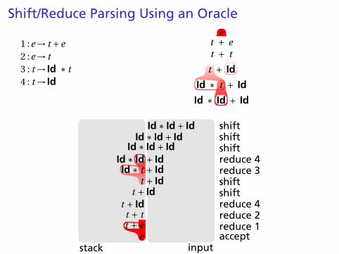
Shift/Reduce Parsing Using an Oracle
1 :e→ t +e2 :e→ t3 : t → Id ∗ t4 : t → Id
et + et + t
t + Id
Id ∗ t + Id
Id ∗ Id + Id
stack input
Id ∗ Id+ Id shiftId ∗ Id+ Id shift
Id ∗ Id+ Id shiftId ∗ Id+ Id reduce 4Id ∗ t + Id reduce 3
t + Id shiftt + Id shift
t + Id reduce 4t + t reduce 2t + e reduce 1
e accept
Handle Hunting
Right Sentential Form: any step in a rightmost derivation
Handle: in a sentential form, a RHS of a rule that, whenrewritten, yields the previous step in a rightmost derivation.
The big question in shift/reduce parsing:
When is there a handle on the top of the stack?
Enumerate all the right-sentential forms and pattern-matchagainst them? Usually infinite in number, but let’s tryanyway.
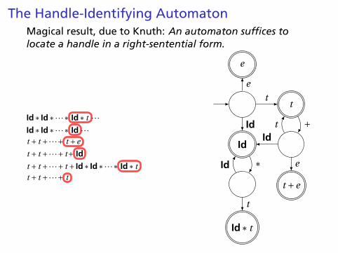
The Handle-Identifying AutomatonMagical result, due to Knuth: An automaton suffices tolocate a handle in a right-sentential form.
Id∗ Id∗·· ·∗ Id∗ t · · ·Id∗ Id∗·· ·∗ Id · · ·t + t +·· ·+ t +e
t + t +·· ·+ t+ Id
t + t +·· ·+ t + Id∗ Id∗·· ·∗ Id∗ t
t + t +·· ·+ t
Id
t
Id∗ t
t +e
e
t
+t
e
IdId
∗Id
t
e
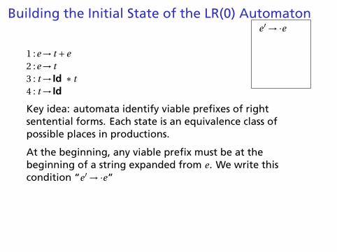
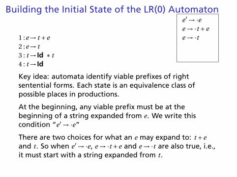
Building the Initial State of the LR(0) Automaton
1 :e→ t +e2 :e→ t3 : t → Id ∗ t4 : t → Id
e ′ →·e
e →·t +ee →·tt →·Id∗ tt →·Id
Key idea: automata identify viable prefixes of rightsentential forms. Each state is an equivalence class ofpossible places in productions.
At the beginning, any viable prefix must be at thebeginning of a string expanded from e. We write thiscondition “e ′ →·e”
There are two choices for what an e may expand to: t +eand t . So when e ′ →·e, e →·t +e and e →·t are also true, i.e.,it must start with a string expanded from t .
Similarly, t must be either Id∗ t or Id, so t →·Id∗ t and t →·Id.
This reasoning is a closure operation like ε-closure in subsetconstruction.
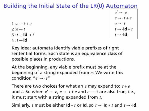
Building the Initial State of the LR(0) Automaton
1 :e→ t +e2 :e→ t3 : t → Id ∗ t4 : t → Id
e ′ →·ee →·t +ee →·t
t →·Id∗ tt →·Id
Key idea: automata identify viable prefixes of rightsentential forms. Each state is an equivalence class ofpossible places in productions.
At the beginning, any viable prefix must be at thebeginning of a string expanded from e. We write thiscondition “e ′ →·e”
There are two choices for what an e may expand to: t +eand t . So when e ′ →·e, e →·t +e and e →·t are also true, i.e.,it must start with a string expanded from t .
Similarly, t must be either Id∗ t or Id, so t →·Id∗ t and t →·Id.
This reasoning is a closure operation like ε-closure in subsetconstruction.
Building the Initial State of the LR(0) Automaton
1 :e→ t +e2 :e→ t3 : t → Id ∗ t4 : t → Id
e ′ →·ee →·t +ee →·tt →·Id∗ tt →·Id
Key idea: automata identify viable prefixes of rightsentential forms. Each state is an equivalence class ofpossible places in productions.
At the beginning, any viable prefix must be at thebeginning of a string expanded from e. We write thiscondition “e ′ →·e”
There are two choices for what an e may expand to: t +eand t . So when e ′ →·e, e →·t +e and e →·t are also true, i.e.,it must start with a string expanded from t .
Similarly, t must be either Id∗ t or Id, so t →·Id∗ t and t →·Id.
This reasoning is a closure operation like ε-closure in subsetconstruction.
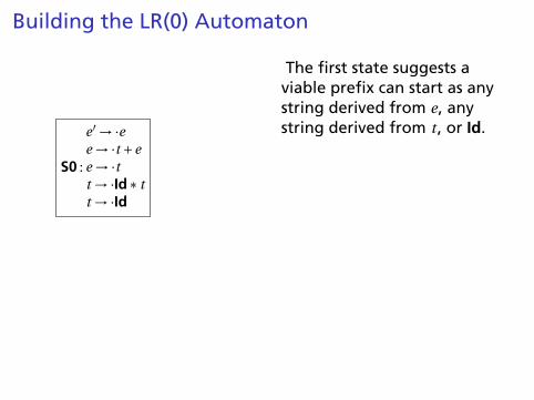
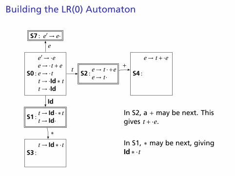
Building the LR(0) Automaton
S0 :
e ′ →·ee →·t +ee →·tt →·Id∗ tt →·Id
S1 :t → Id ·∗tt → Id·
S7 : e ′ → e·
S2 :e → t ·+ee → t ·
e
Id
t
S3 :t → Id∗·t
t →·Id∗ tt →·Id
S4 :
e → t +·e
e →·t +ee →·tt →·Id∗ tt →·Id
∗
+
S5 : t → Id∗ t ·t
Id
S6 : e → t +e·
t
Id e
“Just passed aprefix ending ina string derivedfrom t”
“Just passed aprefix that endedin an Id”
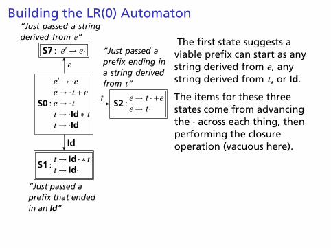
“Just passed a stringderived from e”
The first state suggests aviable prefix can start as anystring derived from e, anystring derived from t , or Id.
The items for these threestates come from advancingthe · across each thing, thenperforming the closureoperation (vacuous here).In S2, a + may be next. Thisgives t +·e.
Closure adds 4more items.
In S1, ∗ may be next, givingId∗·t
and two others.
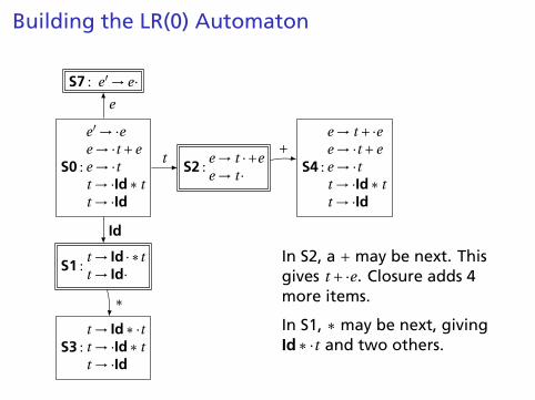
Building the LR(0) Automaton
S0 :
e ′ →·ee →·t +ee →·tt →·Id∗ tt →·Id
S1 :t → Id ·∗tt → Id·
S7 : e ′ → e·
S2 :e → t ·+ee → t ·
e
Id
t
S3 :t → Id∗·t
t →·Id∗ tt →·Id
S4 :
e → t +·e
e →·t +ee →·tt →·Id∗ tt →·Id
∗
+
S5 : t → Id∗ t ·t
Id
S6 : e → t +e·
t
Id e
“Just passed aprefix ending ina string derivedfrom t”
“Just passed aprefix that endedin an Id”
“Just passed a stringderived from e” The first state suggests a
viable prefix can start as anystring derived from e, anystring derived from t , or Id.
The items for these threestates come from advancingthe · across each thing, thenperforming the closureoperation (vacuous here).
In S2, a + may be next. Thisgives t +·e.
Closure adds 4more items.
In S1, ∗ may be next, givingId∗·t
and two others.
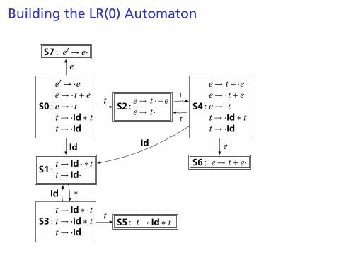
Building the LR(0) Automaton
S0 :
e ′ →·ee →·t +ee →·tt →·Id∗ tt →·Id
S1 :t → Id ·∗tt → Id·
S7 : e ′ → e·
S2 :e → t ·+ee → t ·
e
Id
t
S3 :t → Id∗·t
t →·Id∗ tt →·Id
S4 :
e → t +·e
e →·t +ee →·tt →·Id∗ tt →·Id
∗
+
S5 : t → Id∗ t ·t
Id
S6 : e → t +e·
t
Id e
“Just passed aprefix ending ina string derivedfrom t”
“Just passed aprefix that endedin an Id”
“Just passed a stringderived from e” The first state suggests a
viable prefix can start as anystring derived from e, anystring derived from t , or Id.
The items for these threestates come from advancingthe · across each thing, thenperforming the closureoperation (vacuous here).
In S2, a + may be next. Thisgives t +·e.
Closure adds 4more items.
In S1, ∗ may be next, givingId∗·t
and two others.
Building the LR(0) Automaton
S0 :
e ′ →·ee →·t +ee →·tt →·Id∗ tt →·Id
S1 :t → Id ·∗tt → Id·
S7 : e ′ → e·
S2 :e → t ·+ee → t ·
e
Id
t
S3 :t → Id∗·tt →·Id∗ tt →·Id
S4 :
e → t +·ee →·t +ee →·tt →·Id∗ tt →·Id
∗
+
S5 : t → Id∗ t ·t
Id
S6 : e → t +e·
t
Id e
“Just passed aprefix ending ina string derivedfrom t”
“Just passed aprefix that endedin an Id”
“Just passed a stringderived from e” The first state suggests a
viable prefix can start as anystring derived from e, anystring derived from t , or Id.
The items for these threestates come from advancingthe · across each thing, thenperforming the closureoperation (vacuous here).
In S2, a + may be next. Thisgives t +·e. Closure adds 4more items.
In S1, ∗ may be next, givingId∗·t and two others.
Building the LR(0) Automaton
S0 :
e ′ →·ee →·t +ee →·tt →·Id∗ tt →·Id
S1 :t → Id ·∗tt → Id·
S7 : e ′ → e·
S2 :e → t ·+ee → t ·
e
Id
t
S3 :t → Id∗·tt →·Id∗ tt →·Id
S4 :
e → t +·ee →·t +ee →·tt →·Id∗ tt →·Id
∗
+
S5 : t → Id∗ t ·t
Id
S6 : e → t +e·
t
Id e
“Just passed aprefix ending ina string derivedfrom t”
“Just passed aprefix that endedin an Id”
“Just passed a stringderived from e” The first state suggests a
viable prefix can start as anystring derived from e, anystring derived from t , or Id.
The items for these threestates come from advancingthe · across each thing, thenperforming the closureoperation (vacuous here).In S2, a + may be next. Thisgives t +·e.
Closure adds 4more items.
In S1, ∗ may be next, givingId∗·t
and two others.
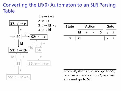
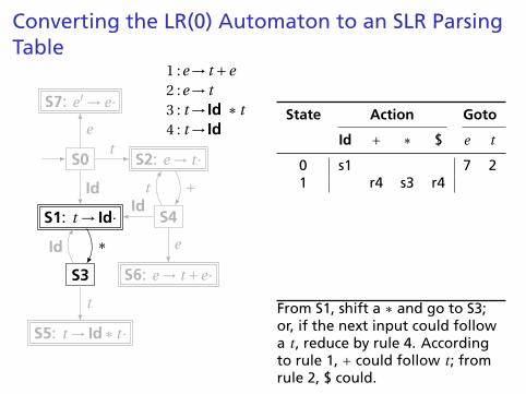
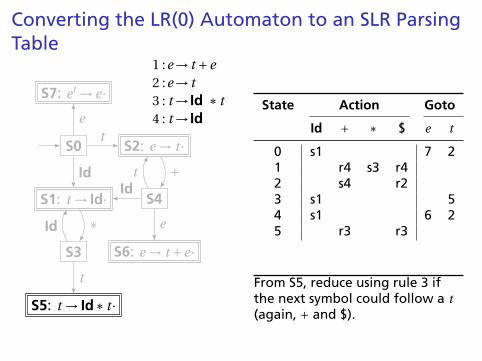
Converting the LR(0) Automaton to an SLR ParsingTable
S0
S1: t → Id·
S2: e → t ·
S3
S4
S5: t → Id∗ t ·
S6: e → t +e·
S7: e ′ → e·
t
Id
e
∗
+
Id
t
t
e
Id
1 :e→ t +e2 :e→ t3 : t → Id ∗ t4 : t → Id
State Action Goto
Id + ∗ $ e t
0 s1 7 2
1 r4 s3 r42 s4 r23 s1 54 s1 6 25 r3 r36 r17 X
From S0, shift an Id and go to S1;or cross a t and go to S2; or crossan e and go to S7.
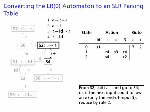
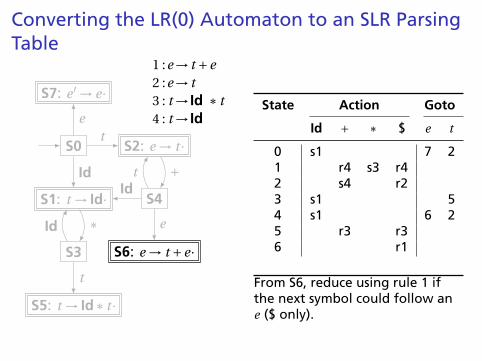
Converting the LR(0) Automaton to an SLR ParsingTable
S0
S1: t → Id·
S2: e → t ·
S3
S4
S5: t → Id∗ t ·
S6: e → t +e·
S7: e ′ → e·
t
Id
e
∗
+
Id
t
t
e
Id
1 :e→ t +e2 :e→ t3 : t → Id ∗ t4 : t → Id
State Action Goto
Id + ∗ $ e t
0 s1 7 21 r4 s3 r4
2 s4 r23 s1 54 s1 6 25 r3 r36 r17 X
From S1, shift a ∗ and go to S3;or, if the next input could followa t , reduce by rule 4. Accordingto rule 1, + could follow t ; fromrule 2, $ could.
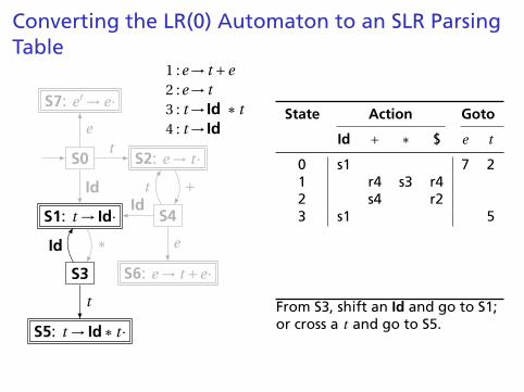
Converting the LR(0) Automaton to an SLR ParsingTable
S0
S1: t → Id·
S2: e → t ·
S3
S4
S5: t → Id∗ t ·
S6: e → t +e·
S7: e ′ → e·
t
Id
e
∗
+
Id
t
t
e
Id
1 :e→ t +e2 :e→ t3 : t → Id ∗ t4 : t → Id
State Action Goto
Id + ∗ $ e t
0 s1 7 21 r4 s3 r42 s4 r2
3 s1 54 s1 6 25 r3 r36 r17 X
From S2, shift a + and go to S4;or, if the next input could followan e (only the end-of-input $),reduce by rule 2.
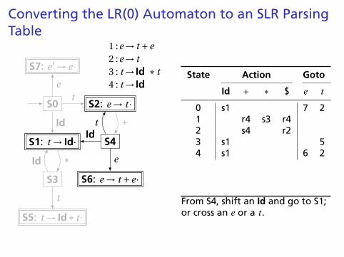
Converting the LR(0) Automaton to an SLR ParsingTable
S0
S1: t → Id·
S2: e → t ·
S3
S4
S5: t → Id∗ t ·
S6: e → t +e·
S7: e ′ → e·
t
Id
e
∗
+
Id
t
t
e
Id
1 :e→ t +e2 :e→ t3 : t → Id ∗ t4 : t → Id
State Action Goto
Id + ∗ $ e t
0 s1 7 21 r4 s3 r42 s4 r23 s1 5
4 s1 6 25 r3 r36 r17 X
From S3, shift an Id and go to S1;or cross a t and go to S5.
Converting the LR(0) Automaton to an SLR ParsingTable
S0
S1: t → Id·
S2: e → t ·
S3
S4
S5: t → Id∗ t ·
S6: e → t +e·
S7: e ′ → e·
t
Id
e
∗
+
Id
t
t
e
Id
1 :e→ t +e2 :e→ t3 : t → Id ∗ t4 : t → Id
State Action Goto
Id + ∗ $ e t
0 s1 7 21 r4 s3 r42 s4 r23 s1 54 s1 6 2
5 r3 r36 r17 X
From S4, shift an Id and go to S1;or cross an e or a t .
Converting the LR(0) Automaton to an SLR ParsingTable
S0
S1: t → Id·
S2: e → t ·
S3
S4
S5: t → Id∗ t ·
S6: e → t +e·
S7: e ′ → e·
t
Id
e
∗
+
Id
t
t
e
Id
1 :e→ t +e2 :e→ t3 : t → Id ∗ t4 : t → Id
State Action Goto
Id + ∗ $ e t
0 s1 7 21 r4 s3 r42 s4 r23 s1 54 s1 6 25 r3 r3
6 r17 X
From S5, reduce using rule 3 ifthe next symbol could follow a t(again, + and $).
Converting the LR(0) Automaton to an SLR ParsingTable
S0
S1: t → Id·
S2: e → t ·
S3
S4
S5: t → Id∗ t ·
S6: e → t +e·
S7: e ′ → e·
t
Id
e
∗
+
Id
t
t
e
Id
1 :e→ t +e2 :e→ t3 : t → Id ∗ t4 : t → Id
State Action Goto
Id + ∗ $ e t
0 s1 7 21 r4 s3 r42 s4 r23 s1 54 s1 6 25 r3 r36 r1
7 X
From S6, reduce using rule 1 ifthe next symbol could follow ane ($ only).

Converting the LR(0) Automaton to an SLR ParsingTable
S0
S1: t → Id·
S2: e → t ·
S3
S4
S5: t → Id∗ t ·
S6: e → t +e·
S7: e ′ → e·
t
Id
e
∗
+
Id
t
t
e
Id
1 :e→ t +e2 :e→ t3 : t → Id ∗ t4 : t → Id
State Action Goto
Id + ∗ $ e t
0 s1 7 21 r4 s3 r42 s4 r23 s1 54 s1 6 25 r3 r36 r17 X
If, in S7, we just crossed an e,accept if we are at the end ofthe input.
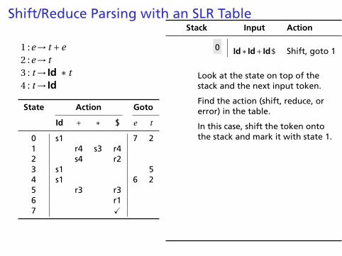
Shift/Reduce Parsing with an SLR Table
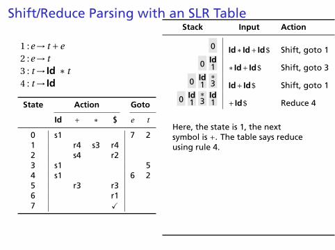
1 :e→ t +e2 :e→ t3 : t → Id ∗ t4 : t → Id
State Action Goto
Id + ∗ $ e t
0 s1 7 21 r4 s3 r42 s4 r23 s1 54 s1 6 25 r3 r36 r17 X
Stack Input Action
0 Id∗ Id+ Id$ Shift, goto 1
Look at the state on top of thestack and the next input token.
Find the action (shift, reduce, orerror) in the table.
In this case, shift the token ontothe stack and mark it with state 1.
0 Id1 ∗ Id+ Id$ Shift, goto 3
0 Id1
∗3 Id+ Id$ Shift, goto 1
0 Id1
∗3
Id1 + Id$ Reduce 4
0 Id1
∗3
t5 + Id$
Reduce 3
0t2 + Id$ Shift, goto 4
0t2
+4 Id$ Shift, goto 1
0t2
+4
Id1 $ Reduce 4
0t2
+4
t2 $ Reduce 2
0t2
+4
e6 $ Reduce 1
0e7 $ Accept
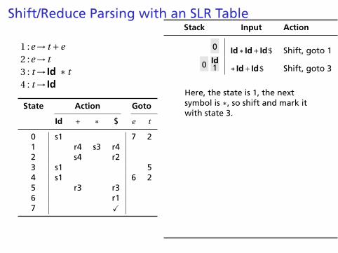
Shift/Reduce Parsing with an SLR Table
1 :e→ t +e2 :e→ t3 : t → Id ∗ t4 : t → Id
State Action Goto
Id + ∗ $ e t
0 s1 7 21 r4 s3 r42 s4 r23 s1 54 s1 6 25 r3 r36 r17 X
Stack Input Action
0 Id∗ Id+ Id$ Shift, goto 1
0 Id1 ∗ Id+ Id$ Shift, goto 3
Here, the state is 1, the nextsymbol is ∗, so shift and mark itwith state 3.
0 Id1
∗3 Id+ Id$ Shift, goto 1
0 Id1
∗3
Id1 + Id$ Reduce 4
0 Id1
∗3
t5 + Id$
Reduce 3
0t2 + Id$ Shift, goto 4
0t2
+4 Id$ Shift, goto 1
0t2
+4
Id1 $ Reduce 4
0t2
+4
t2 $ Reduce 2
0t2
+4
e6 $ Reduce 1
0e7 $ Accept
Shift/Reduce Parsing with an SLR Table
1 :e→ t +e2 :e→ t3 : t → Id ∗ t4 : t → Id
State Action Goto
Id + ∗ $ e t
0 s1 7 21 r4 s3 r42 s4 r23 s1 54 s1 6 25 r3 r36 r17 X
Stack Input Action
0 Id∗ Id+ Id$ Shift, goto 1
0 Id1 ∗ Id+ Id$ Shift, goto 3
0 Id1
∗3 Id+ Id$ Shift, goto 1
0 Id1
∗3
Id1 + Id$ Reduce 4
Here, the state is 1, the nextsymbol is +. The table says reduceusing rule 4.
0 Id1
∗3
t5 + Id$
Reduce 3
0t2 + Id$ Shift, goto 4
0t2
+4 Id$ Shift, goto 1
0t2
+4
Id1 $ Reduce 4
0t2
+4
t2 $ Reduce 2
0t2
+4
e6 $ Reduce 1
0e7 $ Accept
Shift/Reduce Parsing with an SLR Table
1 :e→ t +e2 :e→ t3 : t → Id ∗ t4 : t → Id
State Action Goto
Id + ∗ $ e t
0 s1 7 21 r4 s3 r42 s4 r23 s1 54 s1 6 25 r3 r36 r17 X
Stack Input Action
0 Id∗ Id+ Id$ Shift, goto 1
0 Id1 ∗ Id+ Id$ Shift, goto 3
0 Id1
∗3 Id+ Id$ Shift, goto 1
0 Id1
∗3
Id1 + Id$ Reduce 4
0 Id1
∗3
t5
+ Id$
Reduce 3
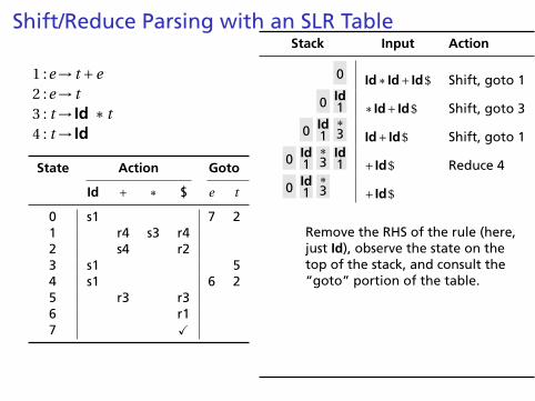
Remove the RHS of the rule (here,just Id), observe the state on thetop of the stack, and consult the“goto” portion of the table.
0t2 + Id$ Shift, goto 4
0t2
+4 Id$ Shift, goto 1
0t2
+4
Id1 $ Reduce 4
0t2
+4
t2 $ Reduce 2
0t2
+4
e6 $ Reduce 1
0e7 $ Accept

Shift/Reduce Parsing with an SLR Table
1 :e→ t +e2 :e→ t3 : t → Id ∗ t4 : t → Id
State Action Goto
Id + ∗ $ e t
0 s1 7 21 r4 s3 r42 s4 r23 s1 54 s1 6 25 r3 r36 r17 X
Stack Input Action
0 Id∗ Id+ Id$ Shift, goto 1
0 Id1 ∗ Id+ Id$ Shift, goto 3
0 Id1
∗3 Id+ Id$ Shift, goto 1
0 Id1
∗3
Id1 + Id$ Reduce 4
0 Id1
∗3
t5 + Id$ Reduce 3
Here, we push a t with state 5.This effectively “backs up” theLR(0) automaton and runs it overthe newly added nonterminal.
In state 5 with an upcoming +,the action is “reduce 3.”
0t2 + Id$ Shift, goto 4
0t2
+4 Id$ Shift, goto 1
0t2
+4
Id1 $ Reduce 4
0t2
+4
t2 $ Reduce 2
0t2
+4
e6 $ Reduce 1
0e7 $ Accept
Shift/Reduce Parsing with an SLR Table
1 :e→ t +e2 :e→ t3 : t → Id ∗ t4 : t → Id
State Action Goto
Id + ∗ $ e t
0 s1 7 21 r4 s3 r42 s4 r23 s1 54 s1 6 25 r3 r36 r17 X
Stack Input Action
0 Id∗ Id+ Id$ Shift, goto 1
0 Id1 ∗ Id+ Id$ Shift, goto 3
0 Id1
∗3 Id+ Id$ Shift, goto 1
0 Id1
∗3
Id1 + Id$ Reduce 4
0 Id1
∗3
t5 + Id$ Reduce 3
0t2 + Id$ Shift, goto 4
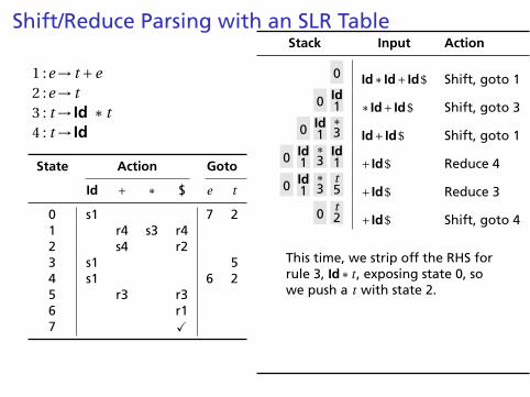
This time, we strip off the RHS forrule 3, Id∗ t , exposing state 0, sowe push a t with state 2.
0t2
+4 Id$ Shift, goto 1
0t2
+4
Id1 $ Reduce 4
0t2
+4
t2 $ Reduce 2
0t2
+4
e6 $ Reduce 1
0e7 $ Accept
Shift/Reduce Parsing with an SLR Table
1 :e→ t +e2 :e→ t3 : t → Id ∗ t4 : t → Id
State Action Goto
Id + ∗ $ e t
0 s1 7 21 r4 s3 r42 s4 r23 s1 54 s1 6 25 r3 r36 r17 X
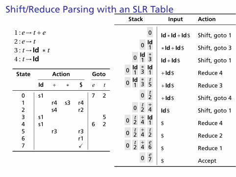
Stack Input Action
0 Id∗ Id+ Id$ Shift, goto 1
0 Id1 ∗ Id+ Id$ Shift, goto 3
0 Id1
∗3 Id+ Id$ Shift, goto 1
0 Id1
∗3
Id1 + Id$ Reduce 4
0 Id1
∗3
t5 + Id$ Reduce 3
0t2 + Id$ Shift, goto 4
0t2
+4 Id$ Shift, goto 1
0t2
+4
Id1 $ Reduce 4
0t2
+4
t2 $ Reduce 2
0t2
+4
e6 $ Reduce 1
0e7 $ Accept
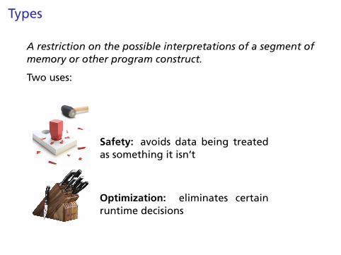
Types
A restriction on the possible interpretations of a segment ofmemory or other program construct.
Two uses:
Safety: avoids data being treatedas something it isn’t
Optimization: eliminates certainruntime decisions
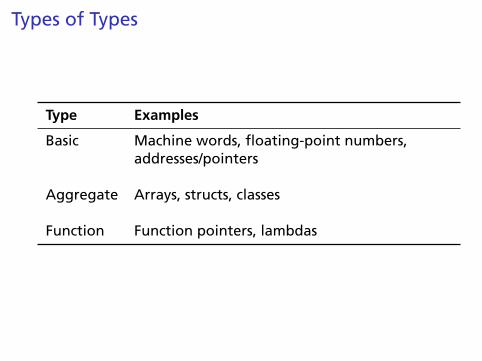
Types of Types
Type Examples
Basic Machine words, floating-point numbers,addresses/pointers
Aggregate Arrays, structs, classes
Function Function pointers, lambdas
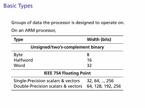
Basic Types
Groups of data the processor is designed to operate on.
On an ARM processor,
Type Width (bits)
Unsigned/two’s-complement binary
Byte 8Halfword 16Word 32
IEEE 754 Floating Point
Single-Precision scalars & vectors 32, 64, .., 256Double-Precision scalars & vectors 64, 128, 192, 256
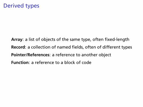
Derived types
Array: a list of objects of the same type, often fixed-length
Record: a collection of named fields, often of different types
Pointer/References: a reference to another object
Function: a reference to a block of code
Structs
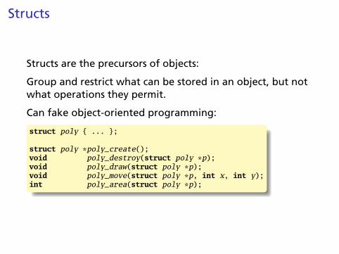
Structs are the precursors of objects:
Group and restrict what can be stored in an object, but notwhat operations they permit.
Can fake object-oriented programming:
struct poly { ... };
struct poly *poly_create();void poly_destroy(struct poly *p);void poly_draw(struct poly *p);void poly_move(struct poly *p, int x, int y);int poly_area(struct poly *p);
Unions: Variant Records
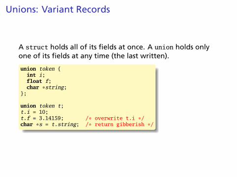
A struct holds all of its fields at once. A union holds onlyone of its fields at any time (the last written).
union token {int i;float f;char *string;
};
union token t;t.i = 10;t.f = 3.14159; /* overwrite t.i */char *s = t.string; /* return gibberish */
Applications of Variant Records
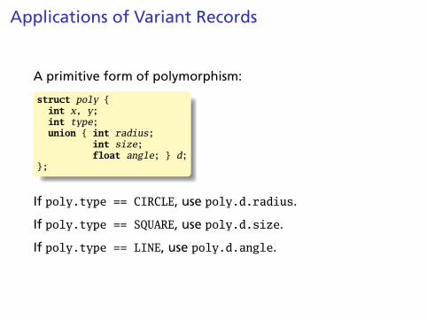
A primitive form of polymorphism:
struct poly {int x, y;int type;union { int radius;
int size;float angle; } d;
};
If poly.type == CIRCLE, use poly.d.radius.
If poly.type == SQUARE, use poly.d.size.
If poly.type == LINE, use poly.d.angle.
Name vs. Structural Equivalence
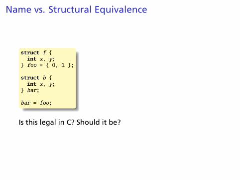
struct f {int x, y;
} foo = { 0, 1 };
struct b {int x, y;
} bar;
bar = foo;
Is this legal in C? Should it be?

Type Expressions
C’s declarators are unusual: they always specify a namealong with its type.
Languages more often have type expressions: a grammarfor expressing a type.
Type expressions appear in three places in C:
(int *) a /* Type casts */sizeof(float [10]) /* Argument of sizeof() */int f(int, char *, int (*)(int)) /* Function argument types */
Basic Static Scope in C, C++, Java, etc.
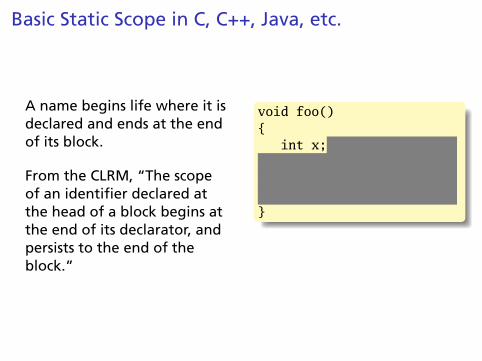
A name begins life where it isdeclared and ends at the endof its block.
From the CLRM, “The scopeof an identifier declared atthe head of a block begins atthe end of its declarator, andpersists to the end of theblock.”
void foo(){
int x;
}
Hiding a Definition
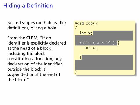
Nested scopes can hide earlierdefinitions, giving a hole.
From the CLRM, “If anidentifier is explicitly declaredat the head of a block,including the blockconstituting a function, anydeclaration of the identifieroutside the block issuspended until the end ofthe block.”
void foo(){
int x;
while ( a < 10 ) {int x;
}
}
Static Scoping in Java
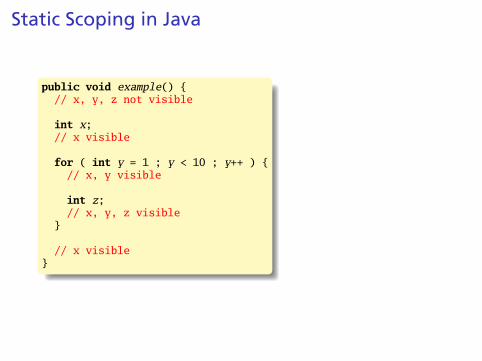
public void example() {// x, y, z not visible
int x;// x visible
for ( int y = 1 ; y < 10 ; y++ ) {// x, y visible
int z;// x, y, z visible
}
// x visible}
Basic Static Scope in O’Caml
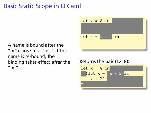
A name is bound after the“in” clause of a “let.” If thename is re-bound, thebinding takes effect after the“in.”
let x = 8 in
let x = x + 1 in
Returns the pair (12, 8):let x = 8 in
(let x = x + 2 inx + 2),
x
Let Rec in O’Caml
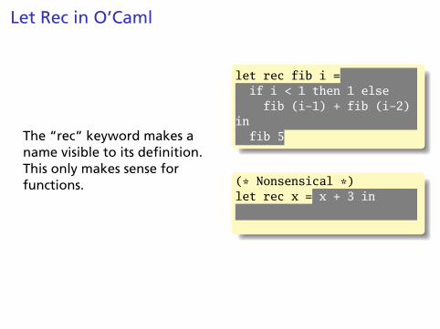
The “rec” keyword makes aname visible to its definition.This only makes sense forfunctions.
let rec fib i =if i < 1 then 1 else
fib (i-1) + fib (i-2)in
fib 5
(* Nonsensical *)let rec x = x + 3 in

Let...and in O’Caml
Let...and lets you bindmultiple names at once.Definitions are not mutuallyvisible unless marked “rec.”
let x = 8and y = 9 in
let rec fac n =if n < 2 then
1else
n * fac1 nand fac1 n = fac (n - 1)infac 5

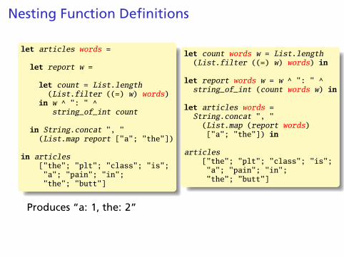
Nesting Function Definitions
let articles words =
let report w =
let count = List.length(List.filter ((=) w) words)
in w ^ ": " ^string_of_int count
in String.concat ", "(List.map report ["a"; "the"])
in articles["the"; "plt"; "class"; "is";"a"; "pain"; "in";"the"; "butt"]
let count words w = List.length(List.filter ((=) w) words) in
let report words w = w ^ ": " ^string_of_int (count words w) in
let articles words =String.concat ", "(List.map (report words)["a"; "the"]) in
articles["the"; "plt"; "class"; "is";"a"; "pain"; "in";"the"; "butt"]
Produces “a: 1, the: 2”
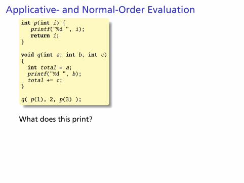
Applicative- and Normal-Order Evaluationint p(int i) {
printf("%d ", i);return i;
}
void q(int a, int b, int c){int total = a;printf("%d ", b);total += c;
}
q( p(1), 2, p(3) );
What does this print?
Applicative: arguments evaluated before function is called.
Result: 1 3 2
Normal: arguments evaluated when used.
Result: 1 2 3
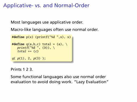
Applicative- vs. and Normal-Order
Most languages use applicative order.
Macro-like languages often use normal order.
#define p(x) (printf("%d ",x), x)
#define q(a,b,c) total = (a), \printf("%d ", (b)), \total += (c)
q( p(1), 2, p(3) );
Prints 1 2 3.
Some functional languages also use normal orderevaluation to avoid doing work. “Lazy Evaluation”
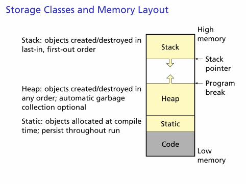
Storage Classes and Memory Layout
Code
StaticStatic: objects allocated at compiletime; persist throughout run
HeapHeap: objects created/destroyed inany order; automatic garbagecollection optional
Programbreak
StackStack: objects created/destroyed inlast-in, first-out order
Stackpointer
Lowmemory
Highmemory
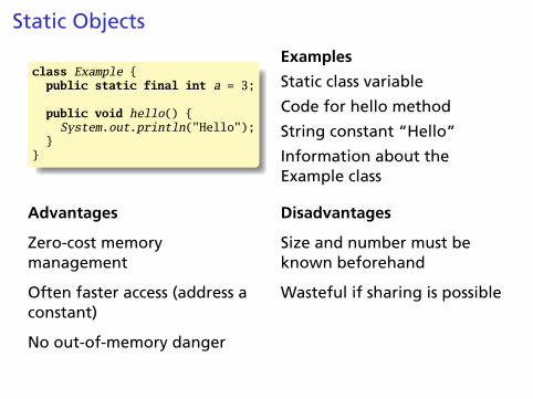
Static Objects
class Example {public static final int a = 3;
public void hello() {System.out.println("Hello");
}}
Examples
Static class variable
Code for hello method
String constant “Hello”
Information about theExample class
Advantages
Zero-cost memorymanagement
Often faster access (address aconstant)
No out-of-memory danger
Disadvantages
Size and number must beknown beforehand
Wasteful if sharing is possible
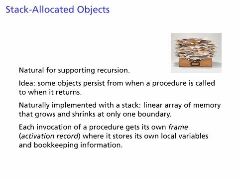
Stack-Allocated Objects
Natural for supporting recursion.
Idea: some objects persist from when a procedure is calledto when it returns.
Naturally implemented with a stack: linear array of memorythat grows and shrinks at only one boundary.
Each invocation of a procedure gets its own frame(activation record) where it stores its own local variablesand bookkeeping information.
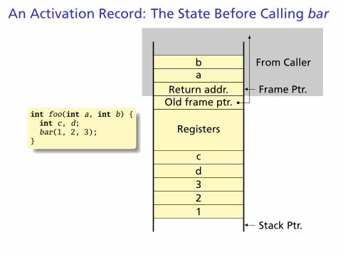
An Activation Record: The State Before Calling bar
int foo(int a, int b) {int c, d;bar(1, 2, 3);
}
From Callerba
Return addr.Old frame ptr.
Registers
cd321
Frame Ptr.
Stack Ptr.
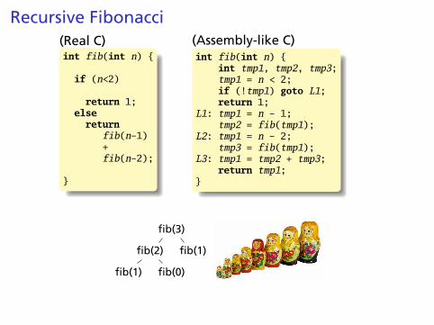
Recursive Fibonacci(Real C)int fib(int n) {
if (n<2)
return 1;elsereturn
fib(n-1)+fib(n-2);
}
(Assembly-like C)int fib(int n) {
int tmp1, tmp2, tmp3;tmp1 = n < 2;if (!tmp1) goto L1;return 1;
L1: tmp1 = n - 1;tmp2 = fib(tmp1);
L2: tmp1 = n - 2;tmp3 = fib(tmp1);
L3: tmp1 = tmp2 + tmp3;return tmp1;
}
fib(3)
fib(2)
fib(1) fib(0)
fib(1)
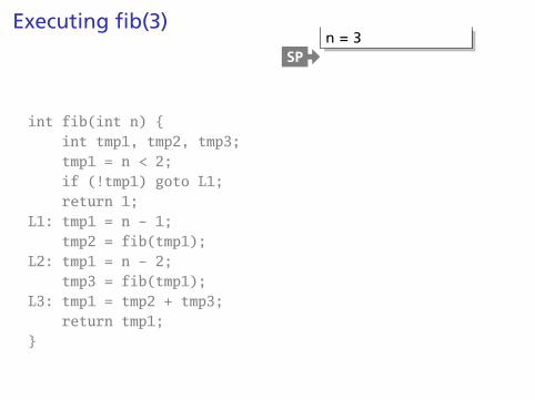
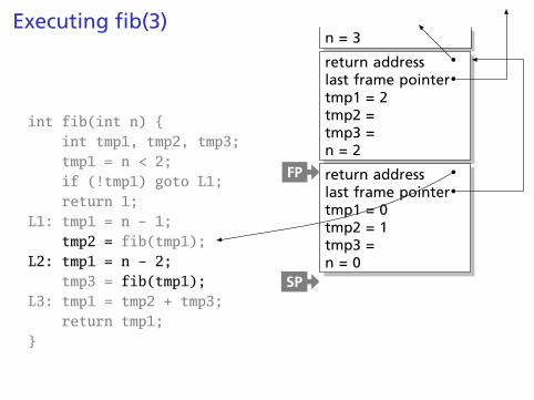
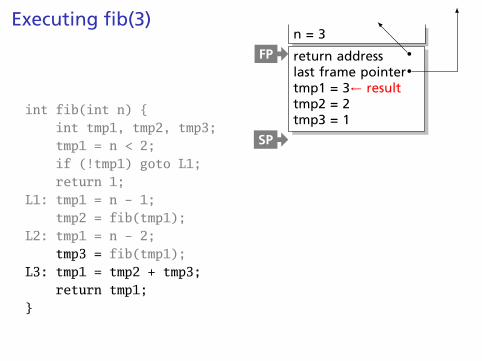
Executing fib(3)
int fib(int n) {int tmp1, tmp2, tmp3;tmp1 = n < 2;if (!tmp1) goto L1;return 1;
L1: tmp1 = n - 1;tmp2 = fib(tmp1);
L2: tmp1 = n - 2;tmp3 = fib(tmp1);
L3: tmp1 = tmp2 + tmp3;return tmp1;
}
n = 3SP
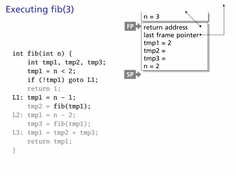
Executing fib(3)
int fib(int n) {int tmp1, tmp2, tmp3;tmp1 = n < 2;if (!tmp1) goto L1;return 1;
L1: tmp1 = n - 1;tmp2 = fib(tmp1);
L2: tmp1 = n - 2;tmp3 = fib(tmp1);
L3: tmp1 = tmp2 + tmp3;return tmp1;
}
n = 3
return addresslast frame pointertmp1 = 2tmp2 =tmp3 =n = 2
FP
SP
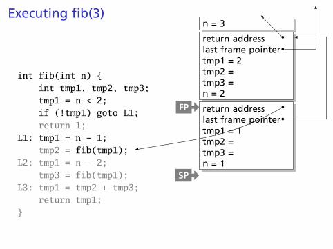
Executing fib(3)
int fib(int n) {int tmp1, tmp2, tmp3;tmp1 = n < 2;if (!tmp1) goto L1;return 1;
L1: tmp1 = n - 1;tmp2 = fib(tmp1);
L2: tmp1 = n - 2;tmp3 = fib(tmp1);
L3: tmp1 = tmp2 + tmp3;return tmp1;
}
n = 3
return addresslast frame pointertmp1 = 2tmp2 =tmp3 =n = 2
return addresslast frame pointertmp1 = 1tmp2 =tmp3 =n = 1
FP
SP
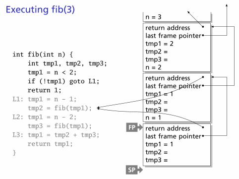
Executing fib(3)
int fib(int n) {int tmp1, tmp2, tmp3;tmp1 = n < 2;if (!tmp1) goto L1;return 1;
L1: tmp1 = n - 1;tmp2 = fib(tmp1);
L2: tmp1 = n - 2;tmp3 = fib(tmp1);
L3: tmp1 = tmp2 + tmp3;return tmp1;
}
n = 3
return addresslast frame pointertmp1 = 2tmp2 =tmp3 =n = 2
return addresslast frame pointertmp1 = 1tmp2 =tmp3 =n = 1
return addresslast frame pointertmp1 = 1tmp2 =tmp3 =
FP
SP
Executing fib(3)
int fib(int n) {int tmp1, tmp2, tmp3;tmp1 = n < 2;if (!tmp1) goto L1;return 1;
L1: tmp1 = n - 1;tmp2 = fib(tmp1);
L2: tmp1 = n - 2;tmp3 = fib(tmp1);
L3: tmp1 = tmp2 + tmp3;return tmp1;
}
n = 3
return addresslast frame pointertmp1 = 2tmp2 =tmp3 =n = 2
return addresslast frame pointertmp1 = 0tmp2 = 1tmp3 =n = 0
FP
SP

Executing fib(3)
int fib(int n) {int tmp1, tmp2, tmp3;tmp1 = n < 2;if (!tmp1) goto L1;return 1;
L1: tmp1 = n - 1;tmp2 = fib(tmp1);
L2: tmp1 = n - 2;tmp3 = fib(tmp1);
L3: tmp1 = tmp2 + tmp3;return tmp1;
}
n = 3
return addresslast frame pointertmp1 = 2tmp2 =tmp3 =n = 2
return addresslast frame pointertmp1 = 0tmp2 = 1tmp3 =n = 0
return addresslast frame pointertmp1 = 1tmp2 =tmp3 =
FP
SP
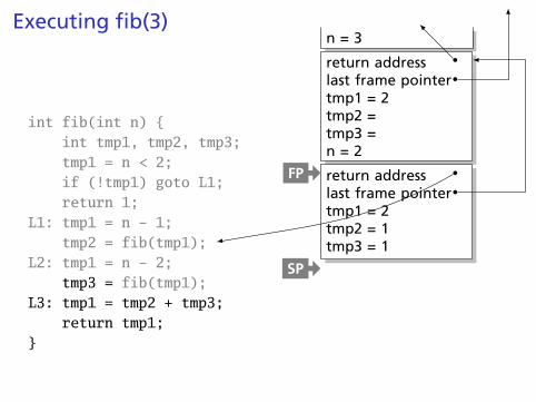
Executing fib(3)
int fib(int n) {int tmp1, tmp2, tmp3;tmp1 = n < 2;if (!tmp1) goto L1;return 1;
L1: tmp1 = n - 1;tmp2 = fib(tmp1);
L2: tmp1 = n - 2;tmp3 = fib(tmp1);
L3: tmp1 = tmp2 + tmp3;return tmp1;
}
n = 3
return addresslast frame pointertmp1 = 2tmp2 =tmp3 =n = 2
return addresslast frame pointertmp1 = 2tmp2 = 1tmp3 = 1
FP
SP
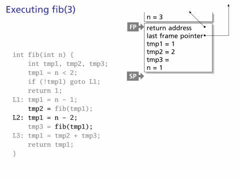
Executing fib(3)
int fib(int n) {int tmp1, tmp2, tmp3;tmp1 = n < 2;if (!tmp1) goto L1;return 1;
L1: tmp1 = n - 1;tmp2 = fib(tmp1);
L2: tmp1 = n - 2;tmp3 = fib(tmp1);
L3: tmp1 = tmp2 + tmp3;return tmp1;
}
n = 3
return addresslast frame pointertmp1 = 1tmp2 = 2tmp3 =n = 1
FP
SP
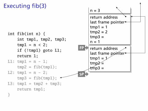
Executing fib(3)
int fib(int n) {int tmp1, tmp2, tmp3;tmp1 = n < 2;if (!tmp1) goto L1;return 1;
L1: tmp1 = n - 1;tmp2 = fib(tmp1);
L2: tmp1 = n - 2;tmp3 = fib(tmp1);
L3: tmp1 = tmp2 + tmp3;return tmp1;
}
n = 3
return addresslast frame pointertmp1 = 1tmp2 = 2tmp3 =n = 1
return addresslast frame pointertmp1 = 1tmp2 =tmp3 =
FP
SP
Executing fib(3)
int fib(int n) {int tmp1, tmp2, tmp3;tmp1 = n < 2;if (!tmp1) goto L1;return 1;
L1: tmp1 = n - 1;tmp2 = fib(tmp1);
L2: tmp1 = n - 2;tmp3 = fib(tmp1);
L3: tmp1 = tmp2 + tmp3;return tmp1;
}
n = 3
return addresslast frame pointertmp1 = 3← resulttmp2 = 2tmp3 = 1
FP
SP
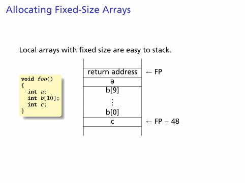
Allocating Fixed-Size Arrays
Local arrays with fixed size are easy to stack.
void foo(){int a;int b[10];int c;
}
return address ← FPa
b[9]...
b[0]c ← FP − 48
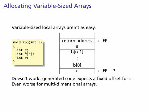
Allocating Variable-Sized Arrays
Variable-sized local arrays aren’t as easy.
void foo(int n){int a;int b[n];int c;
}
return address ← FPa
b[n-1]...
b[0]c ← FP − ?
Doesn’t work: generated code expects a fixed offset for c.Even worse for multi-dimensional arrays.
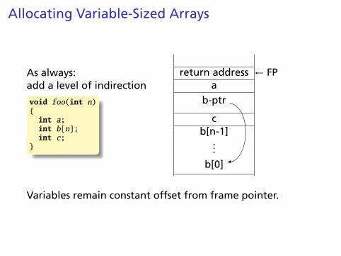
Allocating Variable-Sized Arrays
As always:add a level of indirection
void foo(int n){int a;int b[n];int c;
}
return address ← FPa
b-ptr
cb[n-1]
...b[0]
Variables remain constant offset from frame pointer.
Nesting Function Definitions
let articles words =
let report w =
let count = List.length(List.filter ((=) w) words)
in w ^ ": " ^string_of_int count
in String.concat ", "(List.map report ["a"; "the"])
in articles["the"; "plt"; "class"; "is";"a"; "pain"; "in";"the"; "butt"]
let count words w = List.length(List.filter ((=) w) words) in
let report words w = w ^ ": " ^string_of_int (count words w) in
let articles words =String.concat ", "(List.map (report words)["a"; "the"]) in
articles["the"; "plt"; "class"; "is";"a"; "pain"; "in";"the"; "butt"]
Produces “a: 1, the: 2”
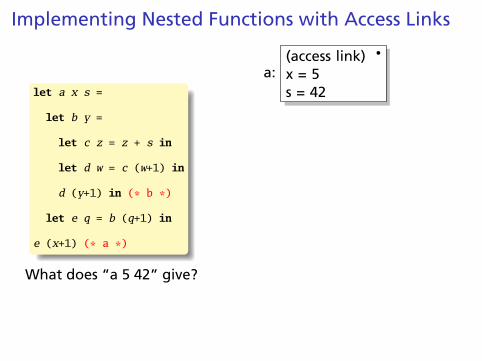
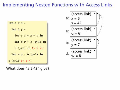
Implementing Nested Functions with Access Links
let a x s =
let b y =
let c z = z + s in
let d w = c (w+1) in
d (y+1) in (* b *)
let e q = b (q+1) in
e (x+1) (* a *)
What does “a 5 42” give?
(access link)x = 5s = 42
a:
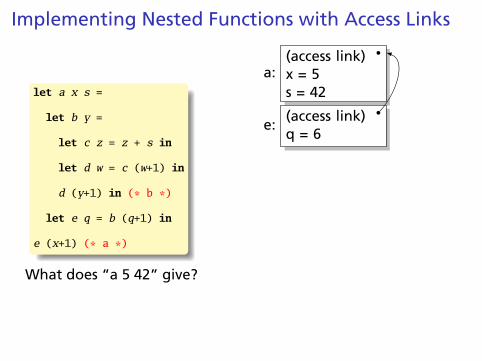
Implementing Nested Functions with Access Links
let a x s =
let b y =
let c z = z + s in
let d w = c (w+1) in
d (y+1) in (* b *)
let e q = b (q+1) in
e (x+1) (* a *)
What does “a 5 42” give?
(access link)x = 5s = 42
a:
(access link)q = 6
e:
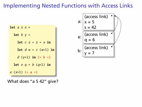
Implementing Nested Functions with Access Links
let a x s =
let b y =
let c z = z + s in
let d w = c (w+1) in
d (y+1) in (* b *)
let e q = b (q+1) in
e (x+1) (* a *)
What does “a 5 42” give?
(access link)x = 5s = 42
a:
(access link)q = 6
e:
(access link)y = 7b:
Implementing Nested Functions with Access Links
let a x s =
let b y =
let c z = z + s in
let d w = c (w+1) in
d (y+1) in (* b *)
let e q = b (q+1) in
e (x+1) (* a *)
What does “a 5 42” give?
(access link)x = 5s = 42
a:
(access link)q = 6
e:
(access link)y = 7b:
(access link)w = 8
d:
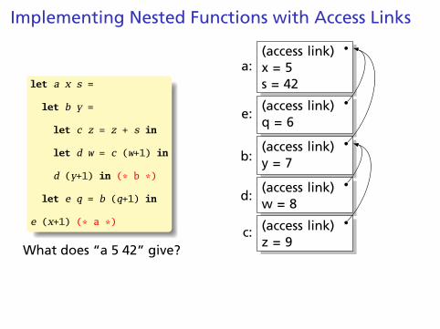
Implementing Nested Functions with Access Links
let a x s =
let b y =
let c z = z + s in
let d w = c (w+1) in
d (y+1) in (* b *)
let e q = b (q+1) in
e (x+1) (* a *)
What does “a 5 42” give?
(access link)x = 5s = 42
a:
(access link)q = 6
e:
(access link)y = 7b:
(access link)w = 8
d:
(access link)z = 9
c:
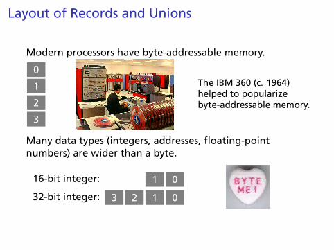
Layout of Records and Unions
Modern processors have byte-addressable memory.
0
1
2
3
The IBM 360 (c. 1964)helped to popularizebyte-addressable memory.
Many data types (integers, addresses, floating-pointnumbers) are wider than a byte.
16-bit integer: 1 0
32-bit integer: 3 2 1 0
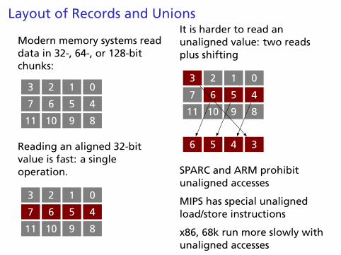
Layout of Records and Unions
Modern memory systems readdata in 32-, 64-, or 128-bitchunks:
3 2 1 0
7 6 5 4
11 10 9 8
Reading an aligned 32-bitvalue is fast: a singleoperation.
3 2 1 0
7 6 5 4
11 10 9 8
It is harder to read anunaligned value: two readsplus shifting
3 2 1 0
7 6 5 4
11 10 9 8
6 5 4 3
SPARC and ARM prohibitunaligned accesses
MIPS has special unalignedload/store instructions
x86, 68k run more slowly withunaligned accesses
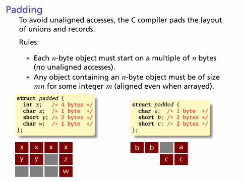
PaddingTo avoid unaligned accesses, the C compiler pads the layoutof unions and records.
Rules:
Ï Each n-byte object must start on a multiple of n bytes(no unaligned accesses).
Ï Any object containing an n-byte object must be of sizemn for some integer m (aligned even when arrayed).
struct padded {int x; /* 4 bytes */char z; /* 1 byte */short y; /* 2 bytes */char w; /* 1 byte */
};
x x x x
y y z
w
struct padded {char a; /* 1 byte */short b; /* 2 bytes */short c; /* 2 bytes */
};
b b a
c c
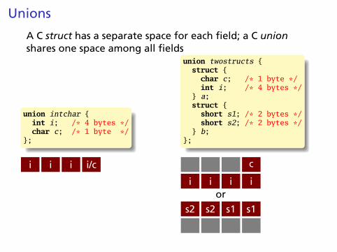
Unions
A C struct has a separate space for each field; a C unionshares one space among all fields
union intchar {int i; /* 4 bytes */char c; /* 1 byte */
};
i i i i/c
union twostructs {struct {
char c; /* 1 byte */int i; /* 4 bytes */
} a;struct {
short s1; /* 2 bytes */short s2; /* 2 bytes */
} b;};
c
i i i ior
s2 s2 s1 s1
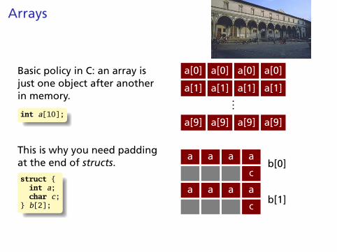
Arrays
Basic policy in C: an array isjust one object after anotherin memory.
int a[10];
a[0] a[0] a[0] a[0]
a[1] a[1] a[1] a[1]
a[9] a[9] a[9] a[9]
...
This is why you need paddingat the end of structs.
struct {int a;char c;
} b[2];
a a a a
c
a a a a
c
b[0]
b[1]
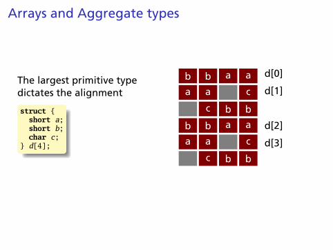
Arrays and Aggregate types
The largest primitive typedictates the alignment
struct {short a;short b;char c;
} d[4];
b b a a
a a c
c b b
b b a a
a a c
c b b
d[0]
d[1]
d[2]
d[3]
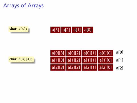
Arrays of Arrays
char a[4]; a[3] a[2] a[1] a[0]
char a[3][4];
a[0][3] a[0][2] a[0][1] a[0][0]
a[1][3] a[1][2] a[1][1] a[1][0]
a[2][3] a[2][2] a[2][1] a[2][0]
a[0]
a[1]
a[2]
Heap-Allocated Storage
Static works when you know everything beforehand andalways need it.
Stack enables, but also requires, recursive behavior.
A heap is a region of memory where blocks can be allocatedand deallocated in any order.
(These heaps are different than those in, e.g., heapsort)
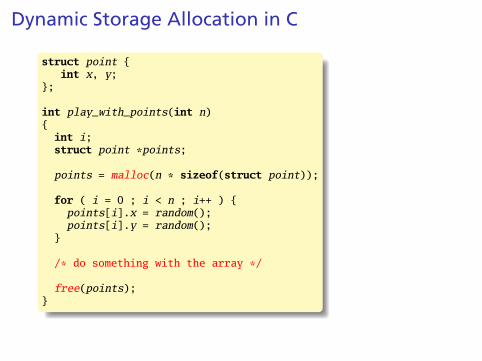
Dynamic Storage Allocation in C
struct point {int x, y;
};
int play_with_points(int n){int i;struct point *points;
points = malloc(n * sizeof(struct point));
for ( i = 0 ; i < n ; i++ ) {points[i].x = random();points[i].y = random();
}
/* do something with the array */
free(points);}
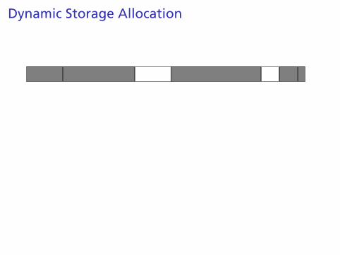
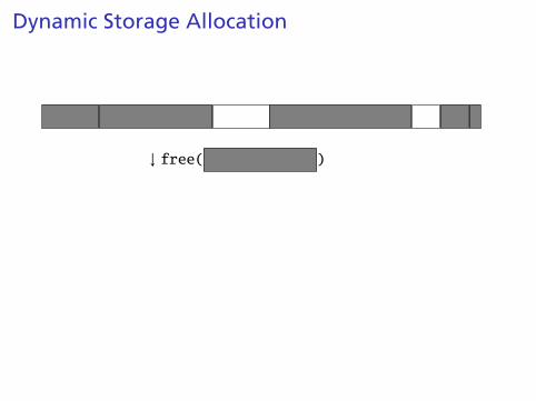
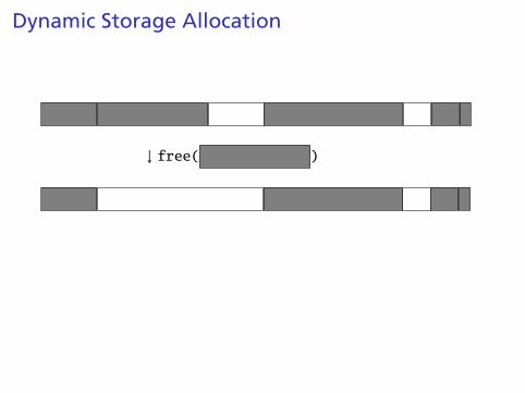
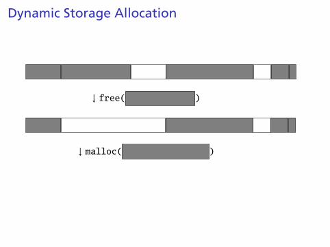
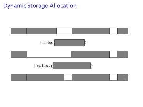
Dynamic Storage Allocation
↓ free( )
↓ malloc( )
Dynamic Storage Allocation
↓ free( )
↓ malloc( )
Dynamic Storage Allocation
↓ free( )
↓ malloc( )
Dynamic Storage Allocation
↓ free( )
↓ malloc( )
Dynamic Storage Allocation
↓ free( )
↓ malloc( )

Dynamic Storage Allocation
Rules:
Each allocated block contiguous (no holes)
Blocks stay fixed once allocated
malloc()
Find an area large enough for requested block
Mark memory as allocated
free()
Mark the block as unallocated
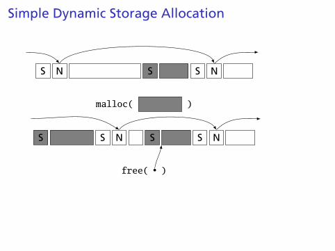
Simple Dynamic Storage Allocation
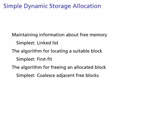
Maintaining information about free memory
Simplest: Linked list
The algorithm for locating a suitable block
Simplest: First-fit
The algorithm for freeing an allocated block
Simplest: Coalesce adjacent free blocks
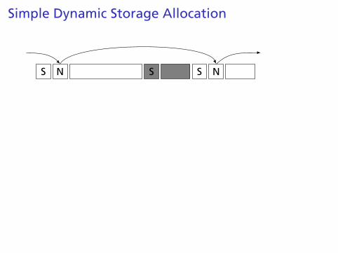
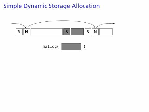
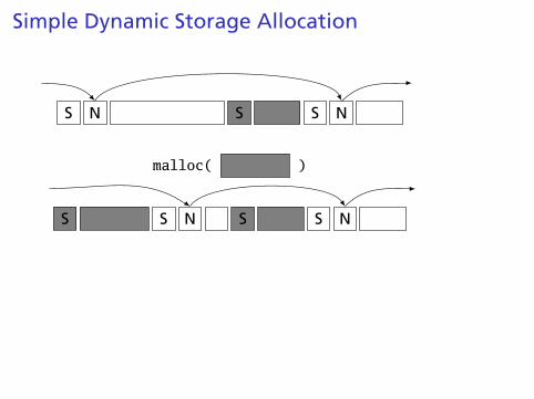
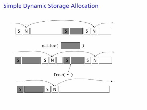
Simple Dynamic Storage Allocation
S N S S N
malloc( )
S S N S S N
free( )
S S N
Simple Dynamic Storage Allocation
S N S S N
malloc( )
S S N S S N
free( )
S S N
Simple Dynamic Storage Allocation
S N S S N
malloc( )
S S N S S N
free( )
S S N
Simple Dynamic Storage Allocation
S N S S N
malloc( )
S S N S S N
free( )
S S N
Simple Dynamic Storage Allocation
S N S S N
malloc( )
S S N S S N
free( )
S S N
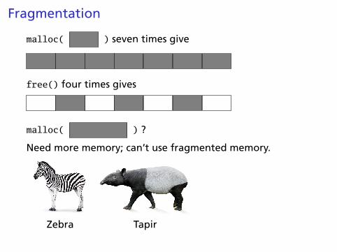
Fragmentation
malloc( ) seven times give
free() four times gives
malloc( ) ?
Need more memory; can’t use fragmented memory.
Zebra Tapir
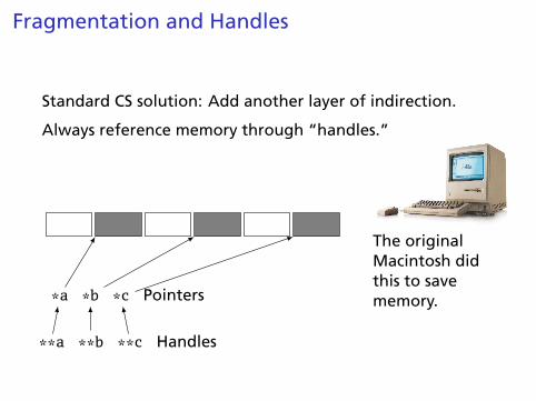
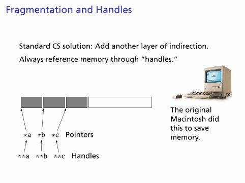
Fragmentation and Handles
Standard CS solution: Add another layer of indirection.
Always reference memory through “handles.”
*a *b *c Pointers
**a **b **c Handles
The originalMacintosh didthis to savememory.
Fragmentation and Handles
Standard CS solution: Add another layer of indirection.
Always reference memory through “handles.”
*a *b *c Pointers
**a **b **c Handles
The originalMacintosh didthis to savememory.
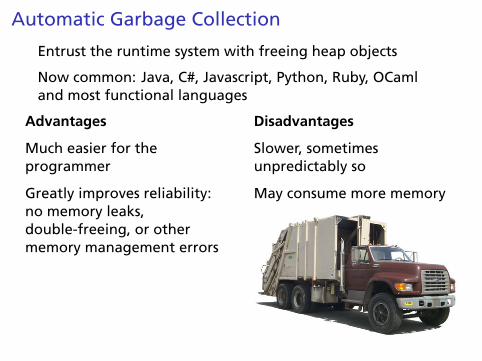
Automatic Garbage Collection
Entrust the runtime system with freeing heap objects
Now common: Java, C#, Javascript, Python, Ruby, OCamland most functional languages
Advantages
Much easier for theprogrammer
Greatly improves reliability:no memory leaks,double-freeing, or othermemory management errors
Disadvantages
Slower, sometimesunpredictably so
May consume more memory

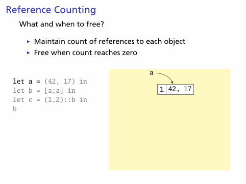
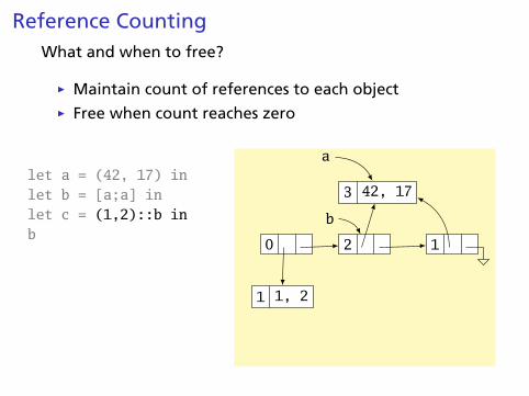
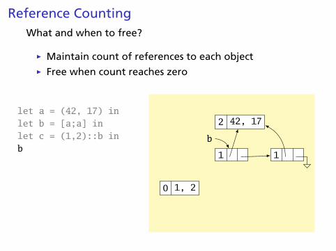
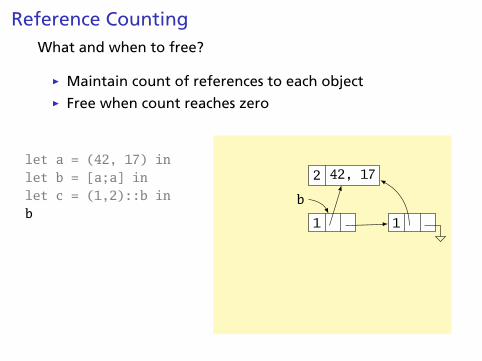
Reference CountingWhat and when to free?
Ï Maintain count of references to each objectÏ Free when count reaches zero
let a = (42, 17) inlet b = [a;a] inlet c = (1,2)::b inb
0 42, 17
Reference CountingWhat and when to free?
Ï Maintain count of references to each objectÏ Free when count reaches zero
let a = (42, 17) inlet b = [a;a] inlet c = (1,2)::b inb
1 42, 17
a
Reference CountingWhat and when to free?
Ï Maintain count of references to each objectÏ Free when count reaches zero
let a = (42, 17) inlet b = [a;a] inlet c = (1,2)::b inb
3 42, 17
a
0 1

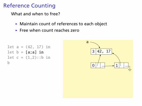
Reference CountingWhat and when to free?
Ï Maintain count of references to each objectÏ Free when count reaches zero
let a = (42, 17) inlet b = [a;a] inlet c = (1,2)::b inb
3 42, 17
a
1 1
b
Reference CountingWhat and when to free?
Ï Maintain count of references to each objectÏ Free when count reaches zero
let a = (42, 17) inlet b = [a;a] inlet c = (1,2)::b inb
3 42, 17
a
2 1
b
1 1, 2
0
Reference CountingWhat and when to free?
Ï Maintain count of references to each objectÏ Free when count reaches zero
let a = (42, 17) inlet b = [a;a] inlet c = (1,2)::b inb
3 42, 17
a
2 1
b
1 1, 2
1
c
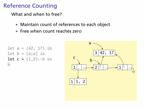
Reference CountingWhat and when to free?
Ï Maintain count of references to each objectÏ Free when count reaches zero
let a = (42, 17) inlet b = [a;a] inlet c = (1,2)::b inb
2 42, 17
2 1
b
1 1, 2
1
c
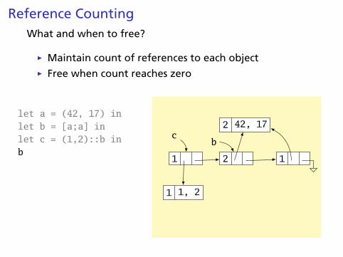
Reference CountingWhat and when to free?
Ï Maintain count of references to each objectÏ Free when count reaches zero
let a = (42, 17) inlet b = [a;a] inlet c = (1,2)::b inb
2 42, 17
2 1
b
1 1, 2
0
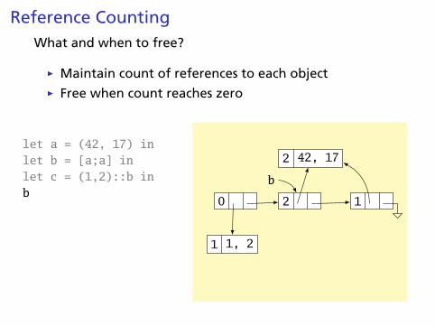
Reference CountingWhat and when to free?
Ï Maintain count of references to each objectÏ Free when count reaches zero
let a = (42, 17) inlet b = [a;a] inlet c = (1,2)::b inb
2 42, 17
1 1
b
0 1, 2
Reference CountingWhat and when to free?
Ï Maintain count of references to each objectÏ Free when count reaches zero
let a = (42, 17) inlet b = [a;a] inlet c = (1,2)::b inb
2 42, 17
1 1
b
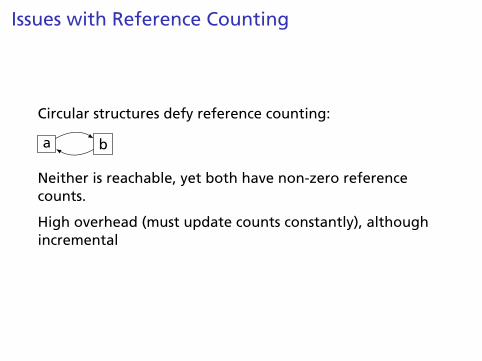
Issues with Reference Counting
Circular structures defy reference counting:
a b
Neither is reachable, yet both have non-zero referencecounts.
High overhead (must update counts constantly), althoughincremental
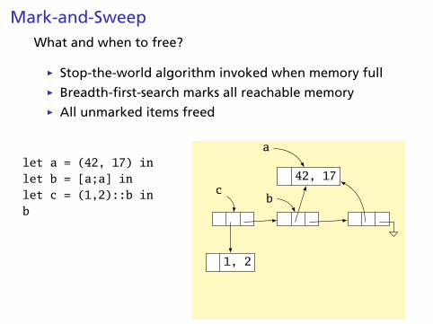
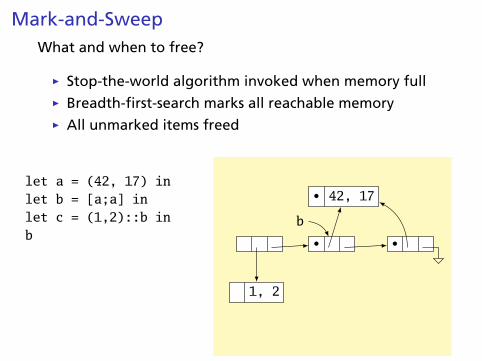
Mark-and-SweepWhat and when to free?
Ï Stop-the-world algorithm invoked when memory fullÏ Breadth-first-search marks all reachable memoryÏ All unmarked items freed
let a = (42, 17) inlet b = [a;a] inlet c = (1,2)::b inb
42, 17
a
b
1, 2
c

Mark-and-SweepWhat and when to free?
Ï Stop-the-world algorithm invoked when memory fullÏ Breadth-first-search marks all reachable memoryÏ All unmarked items freed
let a = (42, 17) inlet b = [a;a] inlet c = (1,2)::b inb
42, 17
•b
1, 2
Mark-and-SweepWhat and when to free?
Ï Stop-the-world algorithm invoked when memory fullÏ Breadth-first-search marks all reachable memoryÏ All unmarked items freed
let a = (42, 17) inlet b = [a;a] inlet c = (1,2)::b inb
• 42, 17
• •b
1, 2
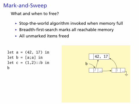
Mark-and-SweepWhat and when to free?
Ï Stop-the-world algorithm invoked when memory fullÏ Breadth-first-search marks all reachable memoryÏ All unmarked items freed
let a = (42, 17) inlet b = [a;a] inlet c = (1,2)::b inb
42, 17
b
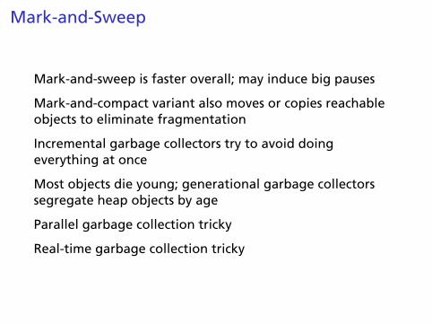
Mark-and-Sweep
Mark-and-sweep is faster overall; may induce big pauses
Mark-and-compact variant also moves or copies reachableobjects to eliminate fragmentation
Incremental garbage collectors try to avoid doingeverything at once
Most objects die young; generational garbage collectorssegregate heap objects by age
Parallel garbage collection tricky
Real-time garbage collection tricky
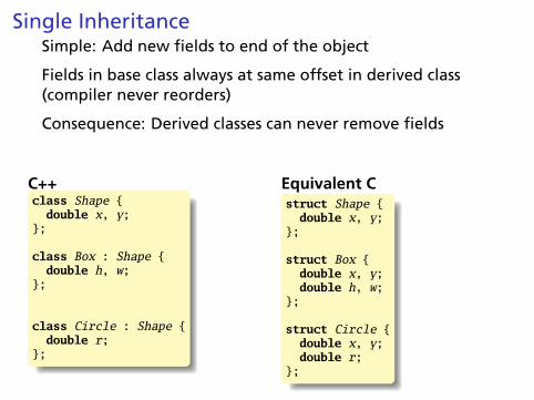
Single InheritanceSimple: Add new fields to end of the object
Fields in base class always at same offset in derived class(compiler never reorders)
Consequence: Derived classes can never remove fields
C++class Shape {double x, y;
};
class Box : Shape {double h, w;
};
class Circle : Shape {double r;
};
Equivalent Cstruct Shape {
double x, y;};
struct Box {double x, y;double h, w;
};
struct Circle {double x, y;double r;
};
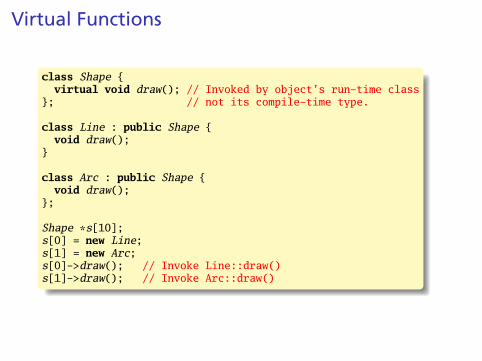
Virtual Functions
class Shape {virtual void draw(); // Invoked by object’s run-time class
}; // not its compile-time type.
class Line : public Shape {void draw();
}
class Arc : public Shape {void draw();
};
Shape *s[10];s[0] = new Line;s[1] = new Arc;s[0]->draw(); // Invoke Line::draw()s[1]->draw(); // Invoke Arc::draw()
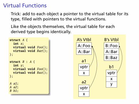
Virtual FunctionsTrick: add to each object a pointer to the virtual table for itstype, filled with pointers to the virtual functions.
Like the objects themselves, the virtual table for eachderived type begins identically.
struct A {int x;virtual void Foo();virtual void Bar();
};
struct B : A {int y;virtual void Foo();virtual void Baz();
};
A a1;A a2;B b1;
A::FooA::Bar
A’s VtblB::FooA::BarB::Baz
B’s Vtbl
vptrx
a1
vptrx
a2
vptrxy
b1
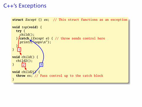
C++’s Exceptions
struct Except {} ex; // This struct functions as an exception
void top(void) {try {child();
} catch (Except e) { // throw sends control hereprintf("oops\n");
}}
void child() {child2();
}
void child2() {throw ex; // Pass control up to the catch block
}
1
2 3
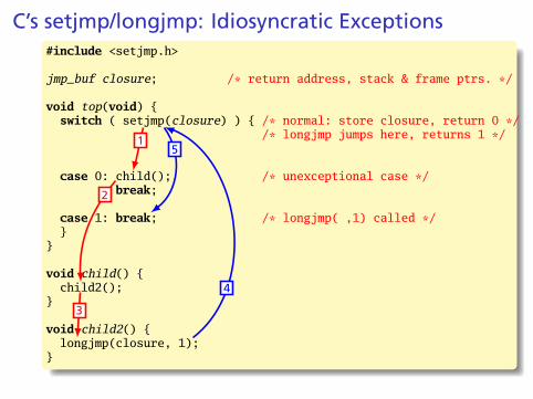
C’s setjmp/longjmp: Idiosyncratic Exceptions#include <setjmp.h>
jmp_buf closure; /* return address, stack & frame ptrs. */
void top(void) {switch ( setjmp(closure) ) { /* normal: store closure, return 0 */
/* longjmp jumps here, returns 1 */
case 0: child(); /* unexceptional case */break;
case 1: break; /* longjmp( ,1) called */}
}
void child() {child2();
}
void child2() {longjmp(closure, 1);
}
1
2
3
4
5
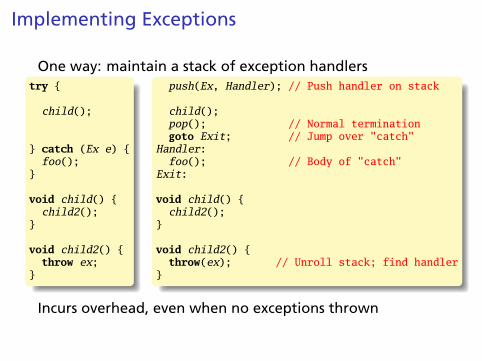
Implementing Exceptions
One way: maintain a stack of exception handlerstry {
child();
} catch (Ex e) {foo();
}
void child() {child2();
}
void child2() {throw ex;
}
push(Ex, Handler); // Push handler on stack
child();pop(); // Normal terminationgoto Exit; // Jump over "catch"
Handler:foo(); // Body of "catch"
Exit:
void child() {child2();
}
void child2() {throw(ex); // Unroll stack; find handler
}
Incurs overhead, even when no exceptions thrown
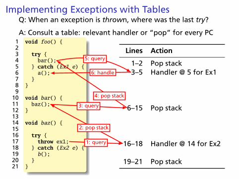
Implementing Exceptions with TablesQ: When an exception is thrown, where was the last try?
A: Consult a table: relevant handler or “pop” for every PC1 void foo() {23 try {4 bar();5 } catch (Ex1 e) {6 a();7 }8 }9
10 void bar() {11 baz();12 }1314 void baz() {1516 try {17 throw ex1;18 } catch (Ex2 e) {19 b();20 }21 }
Lines Action
1–2 Pop stack3–5 Handler @ 5 for Ex1
6–15 Pop stack
16–18 Handler @ 14 for Ex2
19–21 Pop stack
1: query
2: pop stack
3: query
4: pop stack
5: query
6: handle
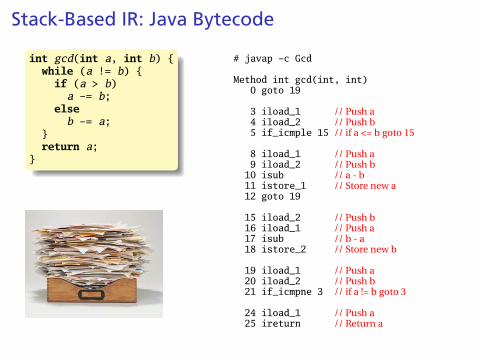
Stack-Based IR: Java Bytecode
int gcd(int a, int b) {while (a != b) {
if (a > b)a -= b;
elseb -= a;
}return a;
}
# javap -c Gcd
Method int gcd(int, int)0 goto 19
3 iload_1 // Push a4 iload_2 // Push b5 if_icmple 15 // if a <= b goto 15
8 iload_1 // Push a9 iload_2 // Push b10 isub // a - b11 istore_1 // Store new a12 goto 19
15 iload_2 // Push b16 iload_1 // Push a17 isub // b - a18 istore_2 // Store new b
19 iload_1 // Push a20 iload_2 // Push b21 if_icmpne 3 // if a != b goto 3
24 iload_1 // Push a25 ireturn // Return a
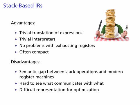
Stack-Based IRs
Advantages:
Ï Trivial translation of expressionsÏ Trivial interpretersÏ No problems with exhausting registersÏ Often compact
Disadvantages:
Ï Semantic gap between stack operations and modernregister machines
Ï Hard to see what communicates with whatÏ Difficult representation for optimization
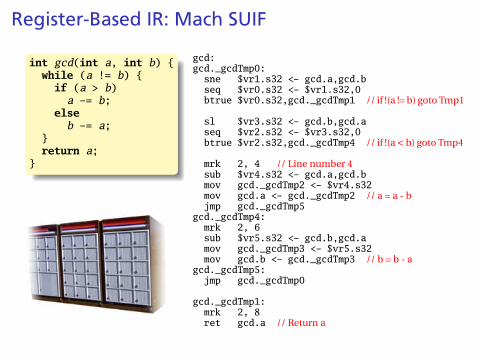
Register-Based IR: Mach SUIF
int gcd(int a, int b) {while (a != b) {
if (a > b)a -= b;
elseb -= a;
}return a;
}
gcd:gcd._gcdTmp0:sne $vr1.s32 <- gcd.a,gcd.bseq $vr0.s32 <- $vr1.s32,0btrue $vr0.s32,gcd._gcdTmp1 // if !(a != b) goto Tmp1
sl $vr3.s32 <- gcd.b,gcd.aseq $vr2.s32 <- $vr3.s32,0btrue $vr2.s32,gcd._gcdTmp4 // if !(a<b) goto Tmp4
mrk 2, 4 // Line number 4sub $vr4.s32 <- gcd.a,gcd.bmov gcd._gcdTmp2 <- $vr4.s32mov gcd.a <- gcd._gcdTmp2 // a = a - bjmp gcd._gcdTmp5
gcd._gcdTmp4:mrk 2, 6sub $vr5.s32 <- gcd.b,gcd.amov gcd._gcdTmp3 <- $vr5.s32mov gcd.b <- gcd._gcdTmp3 // b = b - a
gcd._gcdTmp5:jmp gcd._gcdTmp0
gcd._gcdTmp1:mrk 2, 8ret gcd.a // Return a
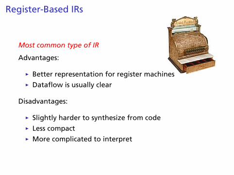
Register-Based IRs
Most common type of IR
Advantages:
Ï Better representation for register machinesÏ Dataflow is usually clear
Disadvantages:
Ï Slightly harder to synthesize from codeÏ Less compactÏ More complicated to interpret
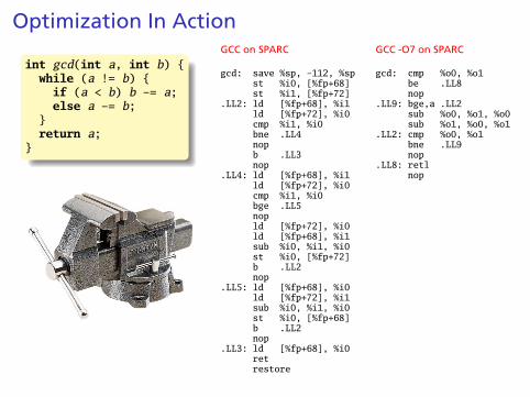
Optimization In Action
int gcd(int a, int b) {while (a != b) {if (a < b) b -= a;else a -= b;
}return a;
}
GCC on SPARC
gcd: save %sp, -112, %spst %i0, [%fp+68]st %i1, [%fp+72]
.LL2: ld [%fp+68], %i1ld [%fp+72], %i0cmp %i1, %i0bne .LL4nopb .LL3nop
.LL4: ld [%fp+68], %i1ld [%fp+72], %i0cmp %i1, %i0bge .LL5nopld [%fp+72], %i0ld [%fp+68], %i1sub %i0, %i1, %i0st %i0, [%fp+72]b .LL2nop
.LL5: ld [%fp+68], %i0ld [%fp+72], %i1sub %i0, %i1, %i0st %i0, [%fp+68]b .LL2nop
.LL3: ld [%fp+68], %i0retrestore
GCC -O7 on SPARC
gcd: cmp %o0, %o1be .LL8nop
.LL9: bge,a .LL2sub %o0, %o1, %o0sub %o1, %o0, %o1
.LL2: cmp %o0, %o1bne .LL9nop
.LL8: retlnop
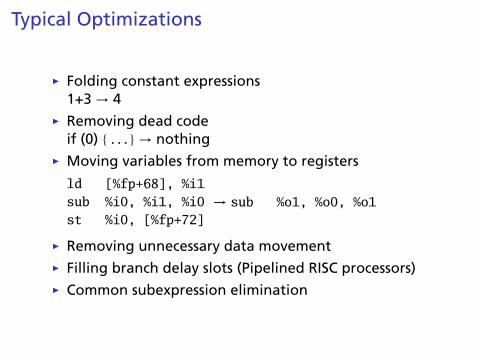
Typical Optimizations
Ï Folding constant expressions1+3 → 4
Ï Removing dead codeif (0) { . . . } → nothing
Ï Moving variables from memory to registers
ld [%fp+68], %i1sub %i0, %i1, %i0st %i0, [%fp+72]
→ sub %o1, %o0, %o1
Ï Removing unnecessary data movementÏ Filling branch delay slots (Pipelined RISC processors)Ï Common subexpression elimination
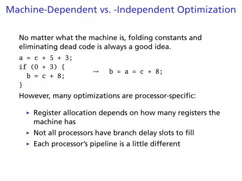
Machine-Dependent vs. -Independent Optimization
No matter what the machine is, folding constants andeliminating dead code is always a good idea.
a = c + 5 + 3;if (0 + 3) {b = c + 8;
}
→ b = a = c + 8;
However, many optimizations are processor-specific:
Ï Register allocation depends on how many registers themachine has
Ï Not all processors have branch delay slots to fillÏ Each processor’s pipeline is a little different
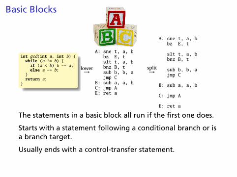
Basic Blocks
int gcd(int a, int b) {while (a != b) {if (a < b) b -= a;else a -= b;
}return a;
}
lower→
A: sne t, a, bbz E, tslt t, a, bbnz B, tsub b, b, ajmp C
B: sub a, a, bC: jmp AE: ret a
split→
A: sne t, a, bbz E, t
slt t, a, bbnz B, t
sub b, b, ajmp C
B: sub a, a, b
C: jmp A
E: ret a
The statements in a basic block all run if the first one does.
Starts with a statement following a conditional branch or isa branch target.
Usually ends with a control-transfer statement.
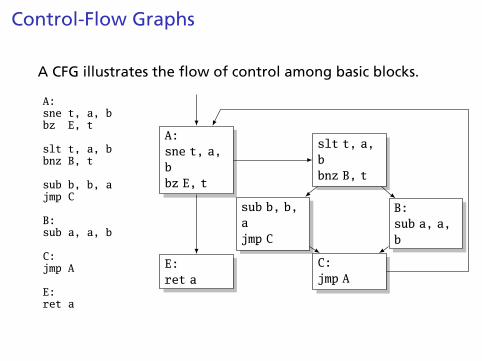
Control-Flow Graphs
A CFG illustrates the flow of control among basic blocks.
A:sne t, a, bbz E, t
slt t, a, bbnz B, t
sub b, b, ajmp C
B:sub a, a, b
C:jmp A
E:ret a
A:sne t, a,bbz E, t
slt t, a,bbnz B, t
sub b, b,ajmp C
B:sub a, a,b
E:ret a
C:jmp A
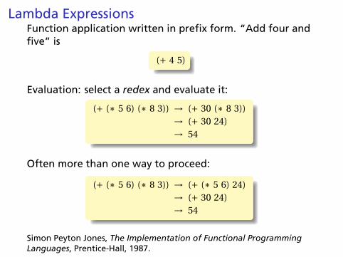
Lambda ExpressionsFunction application written in prefix form. “Add four andfive” is
(+ 4 5)
Evaluation: select a redex and evaluate it:
(+ (∗ 5 6) (∗ 8 3)) → (+ 30 (∗ 8 3))→ (+ 30 24)→ 54
Often more than one way to proceed:
(+ (∗ 5 6) (∗ 8 3)) → (+ (∗ 5 6) 24)→ (+ 30 24)→ 54
Simon Peyton Jones, The Implementation of Functional ProgrammingLanguages, Prentice-Hall, 1987.
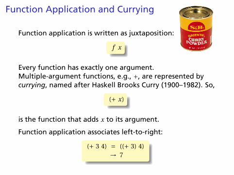
Function Application and Currying
Function application is written as juxtaposition:
f x
Every function has exactly one argument.Multiple-argument functions, e.g., +, are represented bycurrying, named after Haskell Brooks Curry (1900–1982). So,
(+ x)
is the function that adds x to its argument.
Function application associates left-to-right:
(+ 3 4) = ((+ 3) 4)→ 7
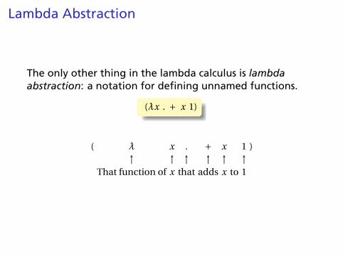
Lambda Abstraction
The only other thing in the lambda calculus is lambdaabstraction: a notation for defining unnamed functions.
(λx . + x 1)
( λ x . + x 1 )↑ ↑ ↑ ↑ ↑ ↑
That function of x that adds x to 1
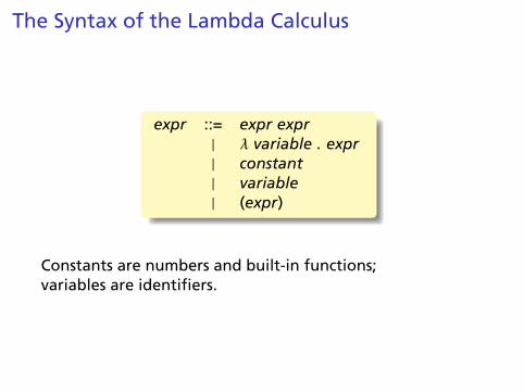
The Syntax of the Lambda Calculus
expr ::= expr expr| λ variable . expr| constant| variable| (expr)
Constants are numbers and built-in functions;variables are identifiers.
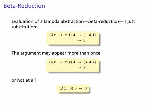
Beta-Reduction
Evaluation of a lambda abstraction—beta-reduction—is justsubstitution:
(λx . + x 1) 4 → (+ 4 1)→ 5
The argument may appear more than once
(λx . + x x) 4 → (+ 4 4)→ 8
or not at all
(λx . 3) 5 → 3
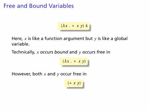
Free and Bound Variables
(λx . + x y) 4
Here, x is like a function argument but y is like a globalvariable.
Technically, x occurs bound and y occurs free in
(λx . + x y)
However, both x and y occur free in
(+ x y)
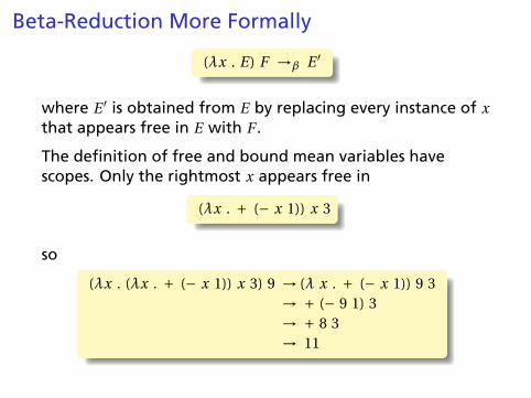
Beta-Reduction More Formally
(λx . E) F →β E ′
where E ′ is obtained from E by replacing every instance of xthat appears free in E with F .
The definition of free and bound mean variables havescopes. Only the rightmost x appears free in
(λx . + (− x 1)) x 3
so
(λx . (λx . + (− x 1)) x 3) 9 → (λ x . + (− x 1)) 9 3→ + (− 9 1) 3→ + 8 3→ 11
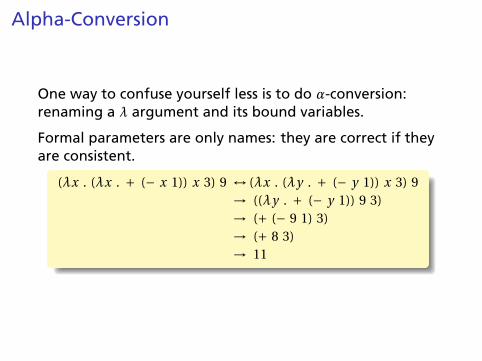
Alpha-Conversion
One way to confuse yourself less is to do α-conversion:renaming a λ argument and its bound variables.
Formal parameters are only names: they are correct if theyare consistent.
(λx . (λx . + (− x 1)) x 3) 9 ↔ (λx . (λy . + (− y 1)) x 3) 9→ ((λy . + (− y 1)) 9 3)→ (+ (− 9 1) 3)→ (+ 8 3)→ 11
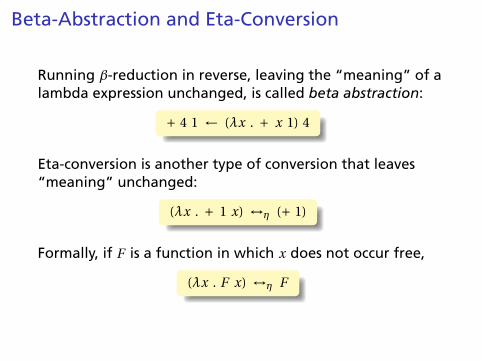
Beta-Abstraction and Eta-Conversion
Running β-reduction in reverse, leaving the “meaning” of alambda expression unchanged, is called beta abstraction:
+ 4 1 ← (λx . + x 1) 4
Eta-conversion is another type of conversion that leaves“meaning” unchanged:
(λx . + 1 x) ↔η (+ 1)
Formally, if F is a function in which x does not occur free,
(λx . F x) ↔η F
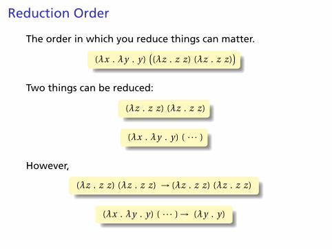
Reduction Order
The order in which you reduce things can matter.
(λx . λy . y)((λz . z z) (λz . z z)
)Two things can be reduced:
(λz . z z) (λz . z z)
(λx . λy . y) ( · · · )
However,
(λz . z z) (λz . z z) → (λz . z z) (λz . z z)
(λx . λy . y) ( · · · ) → (λy . y)
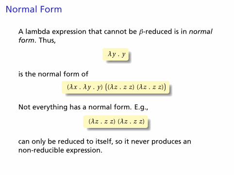
Normal Form
A lambda expression that cannot be β-reduced is in normalform. Thus,
λy . y
is the normal form of
(λx . λy . y)((λz . z z) (λz . z z)
)Not everything has a normal form. E.g.,
(λz . z z) (λz . z z)
can only be reduced to itself, so it never produces annon-reducible expression.
Normal Form
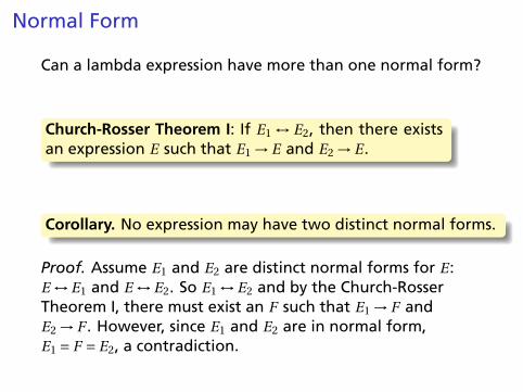
Can a lambda expression have more than one normal form?
Church-Rosser Theorem I: If E1 ↔ E2, then there existsan expression E such that E1 → E and E2 → E .
Corollary. No expression may have two distinct normal forms.
Proof. Assume E1 and E2 are distinct normal forms for E :E ↔ E1 and E ↔ E2. So E1 ↔ E2 and by the Church-RosserTheorem I, there must exist an F such that E1 → F andE2 → F . However, since E1 and E2 are in normal form,E1 = F = E2, a contradiction.
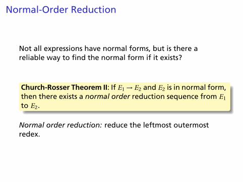
Normal-Order Reduction
Not all expressions have normal forms, but is there areliable way to find the normal form if it exists?
Church-Rosser Theorem II: If E1 → E2 and E2 is in normal form,then there exists a normal order reduction sequence from E1
to E2.
Normal order reduction: reduce the leftmost outermostredex.
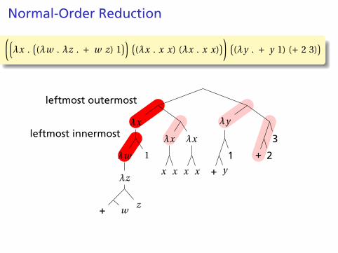
Normal-Order Reduction
((λx .
((λw . λz . + w z) 1
)) ((λx . x x) (λx . x x)
)) ((λy . + y 1) (+ 2 3)
)
leftmost outermost
leftmost innermostλx
λw
λz
+ wz
1
λx
x x
λx
x x
λy
+ y
1 + 2
3
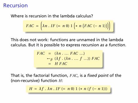
Recursion
Where is recursion in the lambda calculus?
F AC =(λn . I F (= n 0) 1
(∗ n
(F AC (− n 1)
)))
This does not work: functions are unnamed in the lambdacalculus. But it is possible to express recursion as a function.
F AC = (λn . . . . F AC . . .)←β (λ f . (λn . . . . f . . .)) F AC= H F AC
That is, the factorial function, F AC , is a fixed point of the(non-recursive) function H :
H = λ f . λn . I F (= n 0) 1 (∗ n ( f (− n 1)))
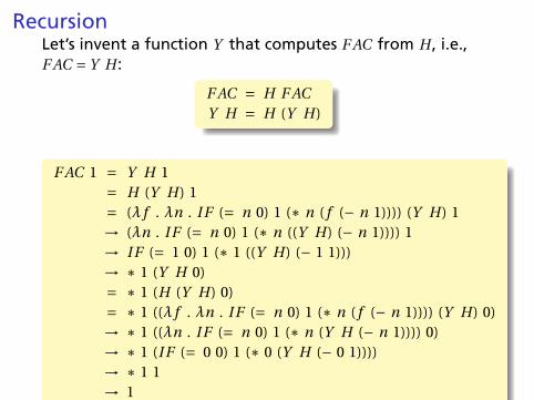
RecursionLet’s invent a function Y that computes F AC from H , i.e.,F AC = Y H :
F AC = H F ACY H = H (Y H)
F AC 1 = Y H 1= H (Y H) 1= (λ f . λn . I F (= n 0) 1 (∗ n ( f (− n 1)))) (Y H) 1→ (λn . I F (= n 0) 1 (∗ n ((Y H) (− n 1)))) 1→ I F (= 1 0) 1 (∗ 1 ((Y H) (− 1 1)))→ ∗ 1 (Y H 0)= ∗ 1 (H (Y H) 0)= ∗ 1 ((λ f . λn . I F (= n 0) 1 (∗ n ( f (− n 1)))) (Y H) 0)→ ∗ 1 ((λn . I F (= n 0) 1 (∗ n (Y H (− n 1)))) 0)→ ∗ 1 (I F (= 0 0) 1 (∗ 0 (Y H (− 0 1))))→ ∗ 1 1→ 1
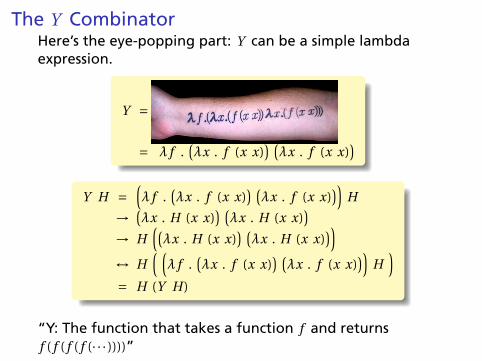
The Y CombinatorHere’s the eye-popping part: Y can be a simple lambdaexpression.
Y =
= λ f .(λx . f (x x)
) (λx . f (x x)
)Y H =
(λ f .
(λx . f (x x)
) (λx . f (x x)
))H
→ (λx . H (x x)
) (λx . H (x x)
)→ H
((λx . H (x x)
) (λx . H (x x)
))↔ H
( (λ f .
(λx . f (x x)
) (λx . f (x x)
))H
)= H (Y H)
“Y: The function that takes a function f and returnsf ( f ( f ( f (· · · ))))”
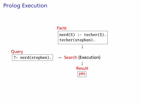
Prolog Execution
Facts
nerd(X) :- techer(X).techer(stephen).
↓Query?- nerd(stephen). → Search (Execution)
↓Result
yes
Simple Searching
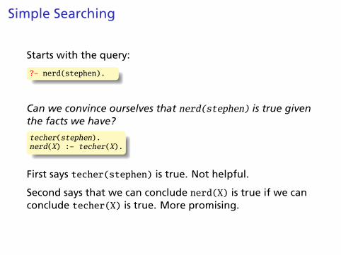
Starts with the query:
?- nerd(stephen).
Can we convince ourselves that nerd(stephen) is true giventhe facts we have?
techer(stephen).nerd(X) :- techer(X).
First says techer(stephen) is true. Not helpful.
Second says that we can conclude nerd(X) is true if we canconclude techer(X) is true. More promising.
Simple Searching
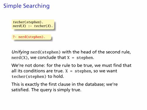
techer(stephen).nerd(X) :- techer(X).
?- nerd(stephen).
Unifying nerd(stephen) with the head of the second rule,nerd(X), we conclude that X = stephen.
We’re not done: for the rule to be true, we must find thatall its conditions are true. X = stephen, so we wanttecher(stephen) to hold.
This is exactly the first clause in the database; we’resatisfied. The query is simply true.
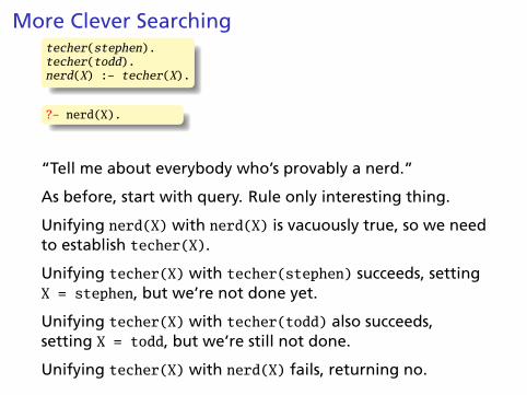
More Clever Searchingtecher(stephen).techer(todd).nerd(X) :- techer(X).
?- nerd(X).
“Tell me about everybody who’s provably a nerd.”
As before, start with query. Rule only interesting thing.
Unifying nerd(X) with nerd(X) is vacuously true, so we needto establish techer(X).
Unifying techer(X) with techer(stephen) succeeds, settingX = stephen, but we’re not done yet.
Unifying techer(X) with techer(todd) also succeeds,setting X = todd, but we’re still not done.
Unifying techer(X) with nerd(X) fails, returning no.
The Prolog Environment
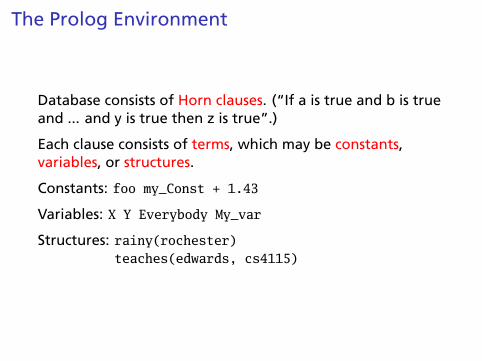
Database consists of Horn clauses. (“If a is true and b is trueand ... and y is true then z is true”.)
Each clause consists of terms, which may be constants,variables, or structures.
Constants: foo my_Const + 1.43
Variables: X Y Everybody My_var
Structures: rainy(rochester)teaches(edwards, cs4115)
Structures and Functors
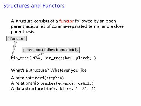
A structure consists of a functor followed by an openparenthesis, a list of comma-separated terms, and a closeparenthesis:
“Functor”
bin_tree(
paren must follow immediately
foo, bin_tree(bar, glarch) )
What’s a structure? Whatever you like.
A predicate nerd(stephen)A relationship teaches(edwards, cs4115)A data structure bin(+, bin(-, 1, 3), 4)
Unification
Part of the search procedure that matches patterns.
The search attempts to match a goal with a rule in thedatabase by unifying them.
Recursive rules:
Ï A constant only unifies with itselfÏ Two structures unify if they have the same functor, the
same number of arguments, and the correspondingarguments unify
Ï A variable unifies with anything but forces anequivalence
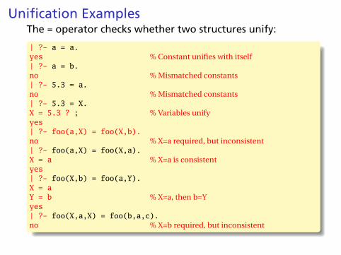
Unification ExamplesThe = operator checks whether two structures unify:
| ?- a = a.yes % Constant unifies with itself| ?- a = b.no % Mismatched constants| ?- 5.3 = a.no % Mismatched constants| ?- 5.3 = X.X = 5.3 ? ; % Variables unifyyes| ?- foo(a,X) = foo(X,b).no % X=a required, but inconsistent| ?- foo(a,X) = foo(X,a).X = a % X=a is consistentyes| ?- foo(X,b) = foo(a,Y).X = aY = b % X=a, then b=Yyes| ?- foo(X,a,X) = foo(b,a,c).no % X=b required, but inconsistent
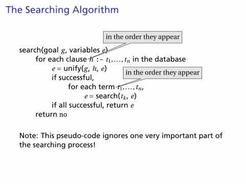
The Searching Algorithm
search(goal g , variables e)for each clause
in the order they appear
h :- t1, . . . , tn in the databasee = unify(g , h, e)if successful,
for each term
in the order they appear
t1, . . . , tn ,e = search(tk , e)
if all successful, return ereturn no
Note: This pseudo-code ignores one very important part ofthe searching process!
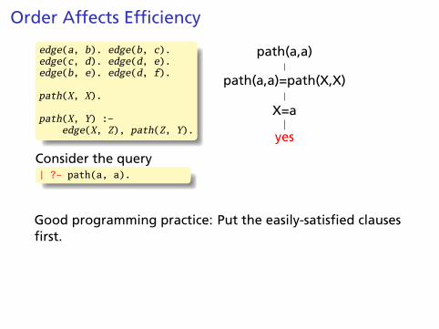
Order Affects Efficiency
edge(a, b). edge(b, c).edge(c, d). edge(d, e).edge(b, e). edge(d, f).
path(X, X).
path(X, Y) :-edge(X, Z), path(Z, Y).
Consider the query| ?- path(a, a).
path(a,a)
path(a,a)=path(X,X)
X=a
yes
Good programming practice: Put the easily-satisfied clausesfirst.
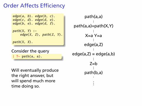
Order Affects Efficiency
edge(a, b). edge(b, c).edge(c, d). edge(d, e).edge(b, e). edge(d, f).
path(X, Y) :-edge(X, Z), path(Z, Y).
path(X, X).
Consider the query| ?- path(a, a).
Will eventually producethe right answer, butwill spend much moretime doing so.
path(a,a)
path(a,a)=path(X,Y)
X=a Y=a
edge(a,Z)
edge(a,Z) = edge(a,b)
Z=b
path(b,a)
...
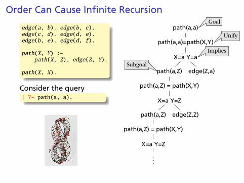
Order Can Cause Infinite Recursion
edge(a, b). edge(b, c).edge(c, d). edge(d, e).edge(b, e). edge(d, f).
path(X, Y) :-path(X, Z), edge(Z, Y).
path(X, X).
Consider the query| ?- path(a, a).
path(a,a)Goal
path(a,a)=path(X,Y)Unify
X=a Y=aImplies
Subgoalpath(a,Z)
path(a,Z) = path(X,Y)
X=a Y=Z
path(a,Z)
path(a,Z) = path(X,Y)
X=a Y=Z
...
edge(Z,Z)
edge(Z,a)
Prolog as an Imperative Language
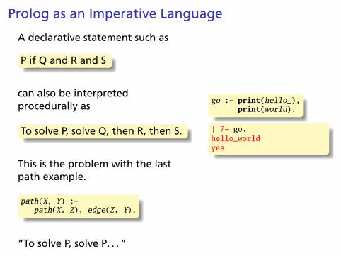
A declarative statement such as
P if Q and R and S
can also be interpretedprocedurally as
To solve P, solve Q, then R, then S.
This is the problem with the lastpath example.
path(X, Y) :-path(X, Z), edge(Z, Y).
“To solve P, solve P. . . ”
go :- print(hello_),print(world).
| ?- go.hello_worldyes
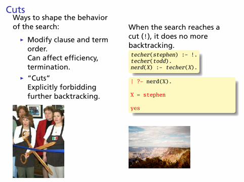
CutsWays to shape the behaviorof the search:
Ï Modify clause and termorder.Can affect efficiency,termination.
Ï “Cuts”Explicitly forbiddingfurther backtracking.
When the search reaches acut (!), it does no morebacktracking.techer(stephen) :- !.techer(todd).nerd(X) :- techer(X).
| ?- nerd(X).
X = stephen
yes