Stepbystepimplementationand ...on-demand.gputechconf.com/gtc-eu/2017/presentation/53028-lokman... · Stepbystepimplementationand optimizationofsimulationsinquantitative ﬁnance LokmanAbbas-Turki

Step by step implementation andoptimization of simulations in quantitativefinance

Lokman Abbas-Turki

UPMC, LPMA

10-12 October 2017

Lokman (UPMC, LPMA) GTC Europe Lab 1 / 28

Plan

Introduction

Local volatilitychallenges GPUs

Monte Carlo andOpenACC

parallelization

Monte Carlo andCUDA parallelization

PDE formulation &Crank-Nicolson

scheme

PDE simulation andCUDA parallelization


Introduction

Plan

Introduction



parallelization



scheme



Introduction

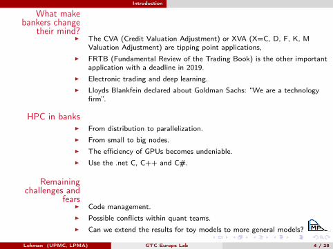
What makebankers change

their mind?I The CVA (Credit Valuation Adjustment) or XVA (X=C, D, F, K, M

Valuation Adjustment) are tipping point applications,I FRTB (Fundamental Review of the Trading Book) is the other important

application with a deadline in 2019.I Electronic trading and deep learning.I Lloyds Blankfein declared about Goldman Sachs: “We are a technology

firm”.

HPC in banksI From distribution to parallelization.I From small to big nodes.I The efficiency of GPUs becomes undeniable.I Use the .net C, C++ and C#.

Remainingchallenges and

fearsI Code management.I Possible conflicts within quant teams.I Can we extend the results for toy models to more general models?


Local volatility challenges GPUs

Plan

Introduction



parallelization



scheme




Local volatility from implied volatilityFirst array: rg dSt = St rg (t)dt + Stσloc (St , t)dWt , S0 = x0.

I S is the stock price process where x0 is the spot priceI W is a Brownian motion with W0 = 0I rg is the risk-free rate, assumed piecewise constantI σloc (x , t) is a local volatility function: R∗+ × R+ → R∗+

Dupire Equation Given a family C(K ,T )K ,T of call prices with strike K and maturity T

σ2loc (K ,T ) = 2

∂C/∂T + Krg (T )∂C/∂K

K2(∂2C/∂K2)

From implied tolocal

Using the Black & Scholes implied volatility σimp(x , t), Andersen andBrotherton-Ratcliffe (1997) showed that

σ2loc (x , t) =

2∂σimp

∂t+σimp

t+ 2xrg (t)

∂σimp

∂x

x2

[∂2σimp

∂x2 − d+

√t

(∂σimp

∂x

)2+

1σimp

(1

x√t

+ d+∂σimp

∂x

)2]

with d+ = 12σimp

√t +

[log(x0/x) +

∫ t0 rg (u)du

]/[σimp

√t]



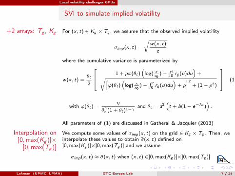
SVI to simulate implied volatility

+2 arrays: Tg , Kg For (x , t) ∈ Kg × Tg , we assume that the observed implied volatility

σimp(x , t) =

√w(x , t)

t

where the cumulative variance is parameterized by

w(x , t) =θt

2

1 + ρϕ(θt)(log( x

x0)−

∫ t0 rg (u)du

)+√[

ϕ(θt)(log( x

x0)−

∫ t0 rg (u)du

)+ ρ]2

+ (1− ρ2)

(1)

with ϕ(θt) =η

θγt (1 + θt)1−γand θt = a2

(t + b(1− e−λt)

).

All parameters of (1) are discussed in Gatheral & Jacquier (2013)

Interpolation on]0,max(Kg )]×]0,max(Tg )]

We compute some values of σimp(x , t) on the grid ∈ Kg × Tg . Then, weinterpolate these values to obtain σ̄(x , t) defined on]0,max(Kg )]×]0,max(Tg )] and we assume

σimp(x , t) ≈ σ̄(x , t) when (x , t) ∈]0,max(Kg )]×]0,max(Tg )]



Bicubic interpolation for implied volatility

Let k , q with (x , t)∈]Kg [k],Kg [k + 1]]×]Tg [q],Tg [q+ 1]]

σ̄(x , t) =3∑

i=0

3∑j=0

Cg (k, q, i , j)l iuj

where l =t − Tg [q]

Tg [q + 1]− Tg [q]and u =

x − Kg [k]

Kg [k + 1]− Kg [k]

Fourth array: Cg Cg (k, q, i , j) = Cg [k ∗ (nt − 1) ∗ 16 + q ∗ 16 + i ∗ 4 + j]

with (k, q, i , j) ∈ {0, ..., nk − 1} × {0, ..., nt − 1} × {0, ..., 3} × {0, ..., 3}and nk , nt are the size of Kg and Tg

Approximated localvolatility

σ2loc (x , t) ≈ min(max(σ̃2(x , t), 0.0001), 0.5)

where σ̃2(x , t) =2∂σ̄

∂t+σ̄

t+ 2xrg (t)

∂σ̄

∂x

x2

[∂2σ̄

∂x2 − d+

√t

(∂σ̄

∂x

)2+

1σ̄

(1

x√t

+ d+∂σ̄

∂x

)2]

with d+ = 12 σ̄√t +

[log(x0/x) +

∫ t0 rg (u)du

]/[σ̄√t]


Monte Carlo and OpenACC parallelization

Plan

Introduction



parallelization



scheme




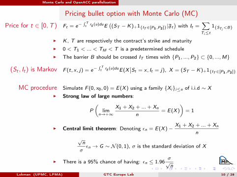
Pricing bullet option with Monte Carlo (MC)

Price for t ∈ [0,T ) Ft = e−∫ Tt rg (u)duE

((ST − K)+1{IT∈[P1,P2]}|Ft

)with It =

∑Ti≤t

1{STi<B}

I K , T are respectively the contract’s strike and maturityI 0 < T1 < ... < TM < T is a predetermined scheduleI The barrier B should be crossed IT times with {P1, ...,P2} ⊂ {0, ...,M}

(St , It) is Markov F (t, x , j) = e−∫ Tt rg (u)duE(X

∣∣St = x , It = j), X = (ST − K)+1{IT∈[P1,P2]} (2)

MC procedure Simulate F (0, x0, 0) = E(X ) using a family {Xi}i≤n of i.i.d ∼ X

I Strong law of large numbers:

P

(lim

n→+∞

X1 + X2 + ...+ Xn

n= E(X )

)= 1

I Central limit theorem: Denoting εn = E(X )−X1 + X2 + ...+ Xn

n√n

σεn → G ∼ N (0, 1), σ is the standard deviation of X

I There is a 95% chance of having: εn ≤ 1.96σ√n



Discritization set 0 = t0 < t1 < ... < tNt = T finer than0 < T1 < ... < TM < T with δt =

√tk+1 − tk

Iterating for path-dependant contract (x0 = 50)

For each tk ,k = 0, ...,Nt−1:

1 Random number generation (RNG) of independent Normal variables Gi

2 Stock price actualization S itk+1

= S itk

(1 + rg (tk )δtδt + σloc (S itk, tk )δtGi )

3 If tk+1 = Tl with l ∈ {1, ...,M}, I iTl= I iTl−1

+ (S iTl< B)

At tNt Compute the payoff X i then average



P. L’Ecuyer CMRG on GPU to generate uniformlydistributed random variables

General Form oflinear RNGs

Without loss of generality:

Xn = (AXn−1 + C) mod(m) = (A : C)

Xn−1. . .1

mod(m) (3)

Parallel-RNG fromPeriod Splitting of

One RNG* Pierre L’Ecuyer proposed a very efficient RNG (1996) which is a CMRG

on 32 bits: Combination of two Multiple Recursive Generator (MRG) withlag = 3 for each MRG.

* Very long period ∼ 2185

xn = (a1xn−1 + a2xn−2 + a3xn−3)mod(m)

Pre-computations We launch as many parallel RNGs as the number of paths

Use We prefer local variables to store the RNG’s state vector



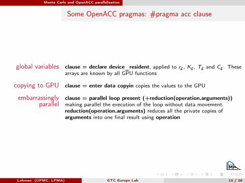
Some OpenACC pragmas: #pragma acc clause

global variables clause = declare device_resident, applied to rg , Kg , Tg and Cg . Thesearrays are known by all GPU functions

copying to GPU clause = enter data copyin copies the values to the GPU

embarrassinglyparallel

clause = parallel loop present (+reduction(operation,arguments))making parallel the execution of the loop without data movement.reduction(operation,arguments) reduces all the private copies ofarguments into one final result using operation


Monte Carlo and CUDA parallelization

Plan

Introduction



parallelization



scheme




GPU architecture

StreamingMultiprocessor

Registers

L1VCache

Constant

Texture

Shared

...L2VCache

{{{

GlobalVMemory{V

V

V

V

V

V...

MemoryVclockedVatVtheVprocessingVrate

ProcessingVunits

CachedVmemory

GPUVRAM


Registers

L1VCache

Constant

Texture

Shared


Registers

L1VCache

Constant

Texture

Shared

Hardware softwareequivalence I Streaming processor: Executes threads

I Streaming multiprocessor: Executes blocks

Built-in variables Known within functions excuted on GPU: threadIdx.x, blockIdx.x,blockDim.x, gridDim.x

Global memory GPU RAM, allocated thanks to cudaMalloc. Transfer values fromGPU/CPU to CPU/GPU thanks to cudaMemcpy

Constant memory Read only, declared globally. Data transfer with cudaMemcpyToSymbol

Shared Declared in the kernelLokman (UPMC, LPMA) GTC Europe Lab 15 / 28


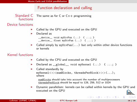
Function declaration and calling

Standard Cfunctions

The same as for C or C++ programming

Device functionsI Called by the GPU and executed on the GPUI Declared as

__device__ void myDivFun (...) { ...; }__device__ float myDivFun (...) { ...; }

I Called simply by myDivFun(...) but only within other device functionsor kernels

Kernel functionsI Called by the CPU and executed on the GPUI Declared as __global__ void myKernel (...) { ...; }I Called standardly by

myKernel<<<numBlocks, threadsPerBlock>>>(...);wherenumBlocks should take into account the number of multiprocessorsthreadsPerBlock should be equal to 128, 256, 512 or 1024

I Dynamic parallelism: kernels can be called within kernels by the GPU andexecuted on the GPU



Adaptation steps

Extension Change it from MC.cpp and rng.cpp to MC.cu and rng.cu

__constant__ Declare Tg , Kg , rg and Cg using constant memory

Copying Copy the values Tg , Kg , rg , Cg and CMRG on the GPU

__device__ Except main, MC, VarMalloc, FreeVar and parameters, define all otherfunctions in MC.cu using __device__

Parallel Declare MC function as a kernel using __global__ + Replace theMonte Carlo loop using threadIdx.x, blockDim.x, blockIdx.x in MC kernel

Reduction Perform the reduction using __shared__ memory in kernel MC andatomicAdd function



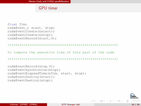
GPU timer

float Tim;cudaEvent_t start, stop;cudaEventCreate(&start);cudaEventCreate(&stop);cudaEventRecord(start,0);

/*******************************************************

To compute the execution time of this part of the code

*******************************************************/

cudaEventRecord(stop,0);cudaEventSynchronize(stop);cudaEventElapsedTime(&Tim, start, stop);cudaEventDestroy(start);cudaEventDestroy(stop);


PDE formulation & Crank-Nicolson scheme

Plan

Introduction



parallelization



scheme




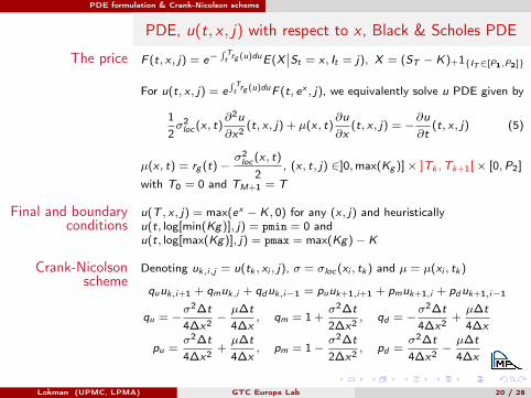
PDE, u(t, x , j) with respect to x , Black & Scholes PDE

The price F (t, x , j) = e−∫ Tt rg (u)duE(X

∣∣St = x , It = j), X = (ST − K)+1{IT∈[P1,P2]} (4)

For u(t, x , j) = e∫ Tt rg (u)duF (t, ex , j), we equivalently solve u PDE given by

12σ2loc (x , t)

∂2u

∂x2 (t, x , j) + µ(x , t)∂u

∂x(t, x , j) = −

∂u

∂t(t, x , j) (5)

µ(x , t) = rg (t)−σ2loc (x , t)

2, (x , t, j) ∈]0,max(Kg )]× ]Tk ,Tk+1[× [0,P2]

with T0 = 0 and TM+1 = T

Final and boundaryconditions

u(T , x , j) = max(ex − K , 0) for any (x , j) and heuristicallyu(t, log[min(Kg)], j) = pmin = 0 andu(t, log[max(Kg)], j) = pmax = max(Kg)− K

Crank-Nicolsonscheme

Denoting uk,i,j = u(tk , xi , j), σ = σloc (xi , tk ) and µ = µ(xi , tk )

quuk,i+1 + qmuk,i + qduk,i−1 = puuk+1,i+1 + pmuk+1,i + pduk+1,i−1

qu = −σ2∆t

4∆x2 −µ∆t

4∆x, qm = 1 +

σ2∆t

2∆x2 , qd = −σ2∆t

4∆x2 +µ∆t

4∆x

pu =σ2∆t

4∆x2 +µ∆t

4∆x, pm = 1−

σ2∆t

2∆x2 , pd =σ2∆t

4∆x2 −µ∆t

4∆x



PDE, u(t, x , j) with respect to j , barrier condition

ut(x , j) = E

(ST − K)+1{∑Mi=1 1{STi <B}∈[P1,P2]

}∣∣∣St = x ,∑Ti≤t

1{STi<B} = j

t ∈ [TM ,T [ ut(x , j) = E[(ST − K)+|St = x]

t ∈ [TM−1,TM ] ut(x , j) = E[(ST − K)+1{STM≥B} | St = x]1{j=P2}

+ E[(ST − K)+1{STM<B} | St = x]1{j=P1−1}

+ E[(ST − K)+|St = x]1{j∈[P1,P2−1]}

[TM−k−1,TM−k ]k = M − 1, ..., 1

(T0 = 0)

ut(x , j) = E[uTM−k(STM−k

,P2)1{STM−k≥B} | St = x]1{j=P2}

+ E[uTM−k(STM−k

, p1k )1{STM−k

<B} | St = x]1{j=p1k−1}

+ E

[uTM−k

(STM−k, j)1{STM−k

≥B}

+uTM−k(STM−k

, j + 1)1{STM−k<B}

∣∣∣St = x

]1{j∈[p1

k,P2−1]}

with p1k = max(P1 − k, 0)




PDE simulation and CUDA parallelization

Plan

Introduction



parallelization



scheme




Solve tridiagonal system for the implicit part

T =

d1 c1

a2 d2 c2 0

a3 d3. . .

. . .. . .

. . .

0. . .

. . . cn−1an dn

.

Cyclic Reduction

e1 e7e5

z2 z8z4 z6

Stepg1:gForwardgreductiongtogag4-unknowngsystemginvolvinggz2,gz4,gz6gandgz8

Stepg2:gForwardgreductiongtoag2-unknowngsystemginvolvinggz4gandgz8

Stepg3:gSolveg2-unknowngsystem

Stepg4:gBackwardgsubstitutiongtosolvegthegrestg2gunknowns

Stepg5:gBackwardgsubstitutiongtosolvegthegrestg4gunknowns

A A A AA AA A

AAA

AAAA

AA

AA

AA

A AAA AAA

AA

AA

A

A

AA

e3

z3z1 z5 z7

e1 e2 e3 e4 e5 e6 e7 e8

e'8e'6e'4e'2

e''4 e''8

e'6e'2 z4 z8

z2 z4 z6 z8



d1 c1c1 d2 c2

c2 d3 c3c3 d4 c4

c4 d5 c5c5 d6 c6

c6 d7

(R)−→

d ′1 0 c ′20 d ′2 0 c ′3c ′2 0 d ′3 0 c ′4

c ′3 0 d ′4 0 c ′5c ′4 0 d ′5 0 c ′6

c ′5 0 d ′6 0c ′6 0 d ′7

(P)−→

d ′1 c ′2c ′2 d ′3 c ′4

c ′4 d ′5 c ′6c ′6 d ′7 0

0 d ′2 c ′3c ′3 d ′4 c ′5

c ′5 d ′6

(R)−→

d ′′1 0 c ′′20 d ′′3 0 c ′′4c ′′2 0 d ′′5 0

c ′′4 0 d ′′7 00 d ′′2 0 c ′′3

0 d ′′4 0c ′′3 0 d ′′6

(P)−→

d ′′1 c ′′2c ′′2 d ′′5 0

0 d ′′3 c ′′4c ′′4 d ′7 0

0 d ′′2 c ′′3c ′′3 d ′′6 0

0 d ′′4



Adaptation steps

Extension Change it from PDE.cpp to PDE.cu

__constant__ Declare Tg , Kg , rg and Cg using constant memory

Copying Copy the values Tg , Kg , rg , Cg on the GPU

__device__ Except for main, PDE_Diff, Out2In, VarMalloc, FreeVar and parameters,define all other functions in PDE.cu using __device__

Registers Compare the CPU version of PCR to the GPU version given to you.Remark the large use of shared memory and registers.

Parallel Declare PDE_Diff and Out2In functions as kernels using __global__ +Replace loops related to St by threadIdx.x and loops related to It byblockIdx.x in PDE_Diff and Out2In kernels as well as in Exp devicefunction.



GPU timer

float Tim;cudaEvent_t start, stop;cudaEventCreate(&start);cudaEventCreate(&stop);cudaEventRecord(start,0);

/*******************************************************

To compute the execution time of this part of the code

*******************************************************/

cudaEventRecord(stop,0);cudaEventSynchronize(stop);cudaEventElapsedTime(&Tim, start, stop);cudaEventDestroy(start);cudaEventDestroy(stop);



ReferencesI L. A. Abbas-Turki, S. Vialle, B. Lapeyre, and P. Mercier. “Pricing

derivatives on graphics processing units using Monte Carlo simulation”.Concurrency and Computation: Practice and Experience, vol. 26(9), pp.1679–1697, 2014.

I L. A. Abbas-Turki and Stef Graillat, “Resolving small random symmetriclinear systems on graphics processing units”, The Journal ofSupercomputing 73(4), pp. 1360–1386, 2017.

I L. B. G. Andersen and R. Brotherton-Ratcliffe, “The equity optionvolatility smile: an implicit finite difference approach”, Journal ofComputational Finance, vol. 1(2), pp. 5–37, 1997.

I J. Gatheral and A. Jacquier, “Arbitrage-free SVI volatility surfaces”,Quantitative Finance, vol. 14(1), pp. 59–71, 2013.

I P. L’Ecuyer, “Combined multiple recursive random number generators”.Operations Research, vol. 44(5), pp. 816–822, 1996.


Documents

Stepbystepimplementationand ...on-demand.gputechconf.com/gtc-eu/2017/presentation/53028-lokman... · Stepbystepimplementationand optimizationofsimulationsinquantitative ﬁnance LokmanAbbas-Turki