Embed Size (px)
Citation preview
StemGL User guide
Fabienne Ribeyre
Marc Jaeger
Alexandre Ribeyre
Philippe de Reffye
marcjaegerciradfr
StemGL at a glance
Cirad Pest amp Disease Unit
Cirad AMAP Unit
httpgreenlabciradfrStemGL
Introduction to StemGL V 13 October 2018 1
1 Introduction bull What is StemGL S3
bull How does StemGL work (GreenLab model General Principles) S4
2 Simulation bull StemGLs simulation approach S5
bull Simulation parameters S6 ndash S17
bull Simulation output S18
3 Fitting bull Fitting principles S20
bull Fitting parameters S21
bull Fitting output (to finalyze) S23
Summary
Introduction to StemGL V 13 October 2018 2
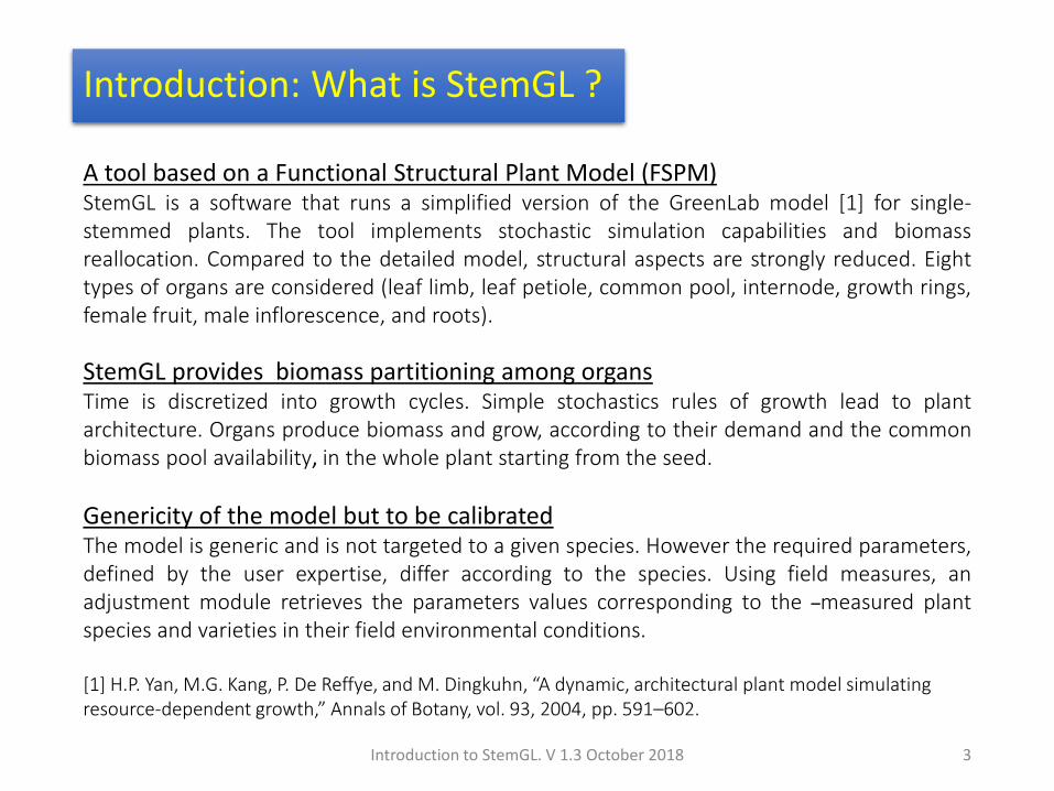
Introduction What is StemGL
A tool based on a Functional Structural Plant Model (FSPM) StemGL is a software that runs a simplified version of the GreenLab model [1] for single-stemmed plants The tool implements stochastic simulation capabilities and biomass reallocation Compared to the detailed model structural aspects are strongly reduced Eight types of organs are considered (leaf limb leaf petiole common pool internode growth rings female fruit male inflorescence and roots)
StemGL provides biomass partitioning among organs Time is discretized into growth cycles Simple stochastics rules of growth lead to plant architecture Organs produce biomass and grow according to their demand and the common biomass pool availability in the whole plant starting from the seed
Genericity of the model but to be calibrated The model is generic and is not targeted to a given species However the required parameters defined by the user expertise differ according to the species Using field measures an adjustment module retrieves the parameters values corresponding to the measured plant species and varieties in their field environmental conditions [1] HP Yan MG Kang P De Reffye and M Dingkuhn ldquoA dynamic architectural plant model simulating resource-dependent growthrdquo Annals of Botany vol 93 2004 pp 591ndash602
Introduction to StemGL V 13 October 2018 3
1 Introduction How does StemGL work
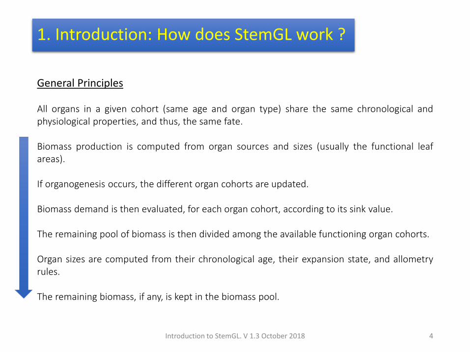
General Principles All organs in a given cohort (same age and organ type) share the same chronological and physiological properties and thus the same fate Biomass production is computed from organ sources and sizes (usually the functional leaf areas) If organogenesis occurs the different organ cohorts are updated Biomass demand is then evaluated for each organ cohort according to its sink value The remaining pool of biomass is then divided among the available functioning organ cohorts Organ sizes are computed from their chronological age their expansion state and allometry rules The remaining biomass if any is kept in the biomass pool
Introduction to StemGL V 13 October 2018 4
2 Simulation StemGLs approach
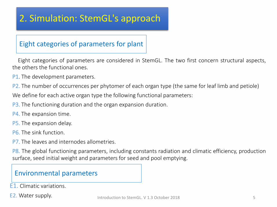
Eight categories of parameters are considered in StemGL The two first concern structural aspects the others the functional ones
P1 The development parameters
P2 The number of occurrences per phytomer of each organ type (the same for leaf limb and petiole)
We define for each active organ type the following functional parameters
P3 The functioning duration and the organ expansion duration
P4 The expansion time
P5 The expansion delay
P6 The sink function
P7 The leaves and internodes allometries
P8 The global functioning parameters including constants radiation and climatic efficiency production surface seed initial weight and parameters for seed and pool emptying
Eight categories of parameters for plant
Introduction to StemGL V 13 October 2018 5
Environmental parameters
E1 Climatic variations
E2 Water supply
Bernoulli probability for developing (b) Bernoulli parameter (b) for stochastic development of stems is characteristic of species and varieties Default b=1 (case of most single-stemmed plants)
Simulation StemGLs input ndash development parameters P1
b=1 Several (N) stochastic realization with b=08 (in this example N=3) it means that for each cycle stem grows with a probability of 08
StemGL gives the user the possibility to represent the simulated plants with the variability induced by the Bernoulli parameter
Introduction to StemGL V 13 October 2018 6
Number of growth cycles T = 10
Ten internodes are produced
Number of growth cycles (T)
Number of growth cycles T = 30 Visualization of graphical results provided by StemGL (under Octavecopy)
Number of cycles realization by the software defined by the last observation date (T gt 0)
Introduction to StemGL V 13 October 2018 7
2 Simulation StemGLs input ndash development parameters P1
Copyright copy 1998-2018 John W Eaton
Rhythm parameters (W W0 and tw) The defaut rhythm ratio is W A change in rhythm parameter is allowed W0 change in W at cycle tw
Except particular cases in StemGL the rhythm parameter W should be set to 1 In all cases 0 lt W lt= 1 Default values W=1 W0=1 tw=0
Interest of rhythm ratios
In GreenLab the rhythm parameter (W) allows to take into account different growth rates between branches and trunk If rhythm parameter of branches is 05 it means that branches grows every two cycles As a consequence the trunk grows twice as fast as the branches
Interest within StemGL taking into account variation of climatic data during one cycle
In the single-stem case (StemGL) the ratio W is not necessary On a single stem W alternates growth period that build phytomer and break period that make void entities The rhythm parameter W induces pauses during which the simulation may use detailed input data (such as climate variations) impacting the plant production
W=1 W=02
Introduction to StemGL V 13 October 2018 8
2 Simulation StemGLs input ndash development parameters P2
(b) T = 30 growth cycles Final age of organogenesis Tm=24
Final age of organogenesis (Tm) After Tm cycles no new organ is created but the existing ones continue to grow and function
(a) T= 30 growth cycles Final age of organogenesis Tm=30
Case (a) Tm ge T 30 internodes are created The last leaf is small because it was created within the last cycle Case (b) Tm lt T 24 internodes are created The last leaf is as big as older ones because it was created 6 cycles ago
Introduction to StemGL V 13 October 2018 9
2 Simulation StemGLs input ndash development parameters P2
Organs contributing to biomass production
The leaf limb is an organ contributing to biomass production In StemGL the petiole and internodes can also contribute to biomass production thanks to remobilization The seed is a stock of biomass released in one or several cycles Common pool is a virtual organ that stocks biomass and may release it
Organs where biomass is allocated Except seed biomass production is allocated to all organs depending of their sink
Biomasse produced at cycle t
Common pool
Leaf (limb + petiole)
Growth ring Male Inflorescence
Fruit
Seed
Internode
Seed
Number of organs no (na nf nm) Organ notations a leaves p petiole i internode c rings f female fruit r root m male inflorescence
The user sets the number of leaves na (same for limb and petiole) the number of fruit nf and the number of male inflorescence nm per internode The internode growth ring and root are considered present if their relative sink is not zero
In StemGL the number of leaves per phytomer is not limited except for the plant display (limited to 2)
Root
Introduction to StemGL V 13 October 2018 10
2 Simulation StemGLs input ndash functioning parameters P2
The functioning duration (tfa tfp tfi tfc tff tfm tft) and the organ expansion duration (txa txp txi txc txf txm txt) for respectively leaves petiole internode growth ring fruit male inflorescence and root
The functioning duration correspond to the number of cycles during which the organ is alive (this is of
importance when the organ may produce or remobilize biomass)
The organ expansion duration correspond to growth
duration (in cycles)
Introduction to StemGL V 13 October 2018 11
2 Simulation StemGLs input ndash functioning parameters P3
The organ expansion duration may vary according to the age of the plant at organ apparition (ontogenic age) Four variation steps are allowed in StemGL
Variation is control by ldquotxo_n_controlrdquo the number of control points for variation in expansions (same for all organs) step1 to step4 number of cycles at which change 1 to 4 occurs User set up for each step organ expansion duration multiplier coefficients that applies to usual txo for leaves petiole internode fruit and male inflorescence The final expansion duration is the usual coefficient txa txp txi txf txm Steps must be age sorted 0 lt step1 lthelliplt step4 lt txo Defaut are txo_n_control = 0
Introduction to StemGL V 13 October 2018 12
2 Simulation StemGLs input ndash function parameters P4ampP5
Sink functions To take into account biomass demand of organs
The demand of organs is defined by organ category (fruit leave growth ring root hellip) They can be constant but generally they are considered as varying during organ development and modelled with a generic function the beta function in StemGL An organ sink function is thus defined for each kind of organ and plant by the two Beta curve parameters
In StemGL sink functions are assumed being the same during the whole plant development
Sink functions are proportional to the leaf one By convention leaves sink function mode is set to 1
Introduction to StemGL V 13 October 2018 13
2 Simulation StemGLs input ndash functioning parameters P6
Sink function shapes varying Beta function parameters with an expansion on 20 cycles
Organ allometries (e b a f parameters) To link the organ fresh biomass to organ dimensions
Organs dimensions are inferred from its biomass increase Fresh biomass is first converted to a volume The relation between this volume and the organ dimensions is defined by an allometry supposed to be stable during growth
Lengthening (b) and shape (a) coefficients internode biomass -gt internode height and section
Introduction to StemGL V 13 October 2018 14
Leaf thickness e leaf biomass -gt leaf area
Fruit density coefficient f Fruit biomass -gt fruit radius r (a=b=1)
2 Simulation StemGLs input ndash functioning parameters P7
Functioning parameters at plant level (EoQoaQoaQr)
Eo overall environmental conditions
Eo qualifies the environmental pressure (default is 1) Decreasing it limits the production in proportion Eo can be defined at various cycles in an external file or expressed as a function (see further)
Qo aQo Plant seed
Qo defines the seed biomass (ie must be gt 0 typical values are 02 to 1 ) Parameter aQo when ne 1 specifies a exponential seed biomass decay The biomass released by the seed dQo at cycle t is expressed as follow dQo(t) = Qo aQo (1 - aQo)(t-1)
aQr Reserve Common Pool
aQr defines the proportion the reserve common pool mobilizes Default value is 0 (no reserve pool) Example with aQr = 075 only frac34 of the common pool are available for organs
Introduction to StemGL V 13 October 2018 15
2 Simulation StemGLs input ndash functioning parameters P8
Functioning parameters at plant level (rSpkc)
r leaf resistivity
R stands for the reversed Water use efficiency Typical values belong to interval [5-20] This value must be set by inverse method (fitting)
Sp Production area
Sp defines the production area (in cm2)
Sp can be understood as the ground projection available for the plant growth When Sp decreases (competition is high) Sp tends to the reversed density (Sd asymp1d) area defines the seed biomass (ie must be gt 0 typical values are 02 to 1 ) Typical values belong to interval [100-10000]
kc LambertBeer law extinction coeficient
The kc parameter is supposed to be constant during plantrsquos life Default value is 1
In practice set Sp according to your stand characteristics keep kc value set to 1 and define r from fitting
Introduction to StemGL V 13 October 2018 16
2 Simulation StemGLs input ndash functioning parameters P8
Detailed Environmental parameters E1
climate global parameters (modE Ec cor wE bE Lmax Lmin)
modE stands for the environmental modes Ec is a global scaling factor cor is a correlation factor wE is a rhythm bE a probability and Lmax and Lmin are light limit values
for modE = 1 we have E(t) = Eo (constant default) for each cycle t
for modE = 2 we have E(t) is random with autocorrelation
E(1) = Ec and then E(tgt1) = cor E(t-1) + (1-cor) (Lmin + random (Lmax-Lmin))
for modE = 3 we have E(t) is periodic with values 0 and Ec with rhythm wE and probability bE
Example (mode comparison) with Ec = 08 cor = 02Lmax = 25 Lmin = 05 wE = 3 bE = 025
Introduction to StemGL V 13 October 2018 17
2 Simulation StemGLs input ndash Environmental parameters
modE = 1 modE = 2 modE = 3
Detailed Environmental parameters E2
Water supply parameters (modH c1 c2 Hmx Hmn H1_psi_pH20_dH20)
modH c1 c2 Hmx Hmn H1_psi_pH20_dH20
modH stands for the water supply mode and frequencies
for modH = 0 we have no irrigation DH(1T) = 0
for modH = -1 we have random irrigation DH(1T) = randomdH20 (if random lt pH20)
for modH gt 0 we have regular irrigation DH(1T) = dH20 (1 - sign(mod(tmodH)))
The water availability model
H(1) = H1 water availability at first cycle
then H(i) = H(i-1) - (SfSp) c1 (H(i-1) -Hmn) + c2 (Hmx- H(i-1)) DH(i1)
c1 and c2 are two coefficients standing for the plant water uptake and the soil absorption respectively
Introduction to StemGL V 13 October 2018 18
2 Simulation StemGLs input ndash Environmental parameters
Information in the command console
During simulation
Files loaded names (parameters mask hellip) and eventually an error message (file error or data error)
At each growth cycle Cycle Biomass (cumulated increment leaf internode fruit) are given
Example (with 28 cycles) C1 Biomass0046236(0046236) leaf0015082 internode0002558 fruit0000000
helliphellip
C28 Biomass148344551(2609407942) leaf273070718 internode207233293 fruit1784252201
Computing time performances (at end of simulation for each task) Example
TOTAL CPU TIME 3984375 Total simulation 0187500
----------------------------------------------------------
Parameter loading 0031250 Development Axis 0015625
Mask load amp apply 0015625 Climate model 0000000
Organ durations 0000000 Sink Organ Beta laws 0015625
Plant Organ demand 0015625 Plant Organ growth 0109375
Organic series 0031250 Plotting results 0968750
Plant Display 0250000 Target amp Mask save 0015625
2 Simulation StemGLs output
Introduction to StemGL V 13 October 2018 19
Organ expansion and sink functions
Plant functioning results (cycle)
Climate factor number of phytomers
demand biomass production
Biomass allocated to organ componants
Organ chronological and topological series
biomass curves including those at observation times
Plant chronological and topological structure representations
Graphical diagrams (displayed at end of simulation)
2 Simulation StemGLs output Curves
Introduction to StemGL V 13 October 2018 20
Given parameters and fitted parameters
Structural development parameters
Structural parameters (development probability rhythm ratio viability hellip) must be given They can be estimated from field internode distribution statistical analysis Typically the mean variance ratio is used to estimate Bernoulli parameter b
Functional parameters to be given
The following parameters must be given Expansion and functioning times Surface of production and Organ allometries
Functional parameters to be fitted
Global functioning parameters (Qo r)
Organ sink functions (beta law parameters)
3 Fitting Principles
Introduction to StemGL V 13 October 2018 21
Data collection modes amp fitting parameters
Data collection modes (comp phyt)
Measures can be given per compartment orand per phytomer
Comp=1 stands for global organ compartment level (default 1)
Phyt=1 stands for local organ compartment level (phytomer level) (default 1)
Fitting parameters are predefined (they can be changed in the interpreted code)
The fitting method is the generalized least square method
The number of iterations is set to 10 (by default)
3 Fitting StemGLs input ndash Parameters F1
22
At least one collection mode must be active
Introduction to StemGL V 13 October 2018
Parameter selection
Selected parameters have their selector set to value 1
Unselected parameters have their selector set to value 0
Parameter that can be fitted
xQo xaQo xr xSp global functional parameters
Xpp xpi xpc xpf xpm xpt kpc kpa kpi Sink functions
xBa1 xBp1 xBi1 xBf1 xBm1 xBt1 xBa2 xBp2 xBi2 xBf2 xBm2 xBt2 Expansion Beta law parameters (two parameter per organ type)
3 Fitting StemGLs input ndash Parameters F2
23
At least one parameter selector must be active
Trick the parameter selector name is the parameter name prefixed by letter lsquoxrsquo
Example xSp is the selector of Parameter Sp
Introduction to StemGL V 13 October 2018
During simulation
Files loaded names (parameters mask hellip) and eventually an error message (file error or data error)
At each iteration the list of parameters values issued and the error The two last lines print the estimated parameter values (A) and their standard deviation (sA) Example
13047 2421442 1000 0500 25003 0700 1500 3000 3000 3000 iter = 3 error = 674794
helliphellip
12013 2221031 1024 0612 22673 0768 1738 3460 3037 3372 iter = 10 error = 151926
xr____xSp___xpp___xpe___xpf___xkpa__xkpe__xBa1__xBp1__xBi1__
A 1=1201 A 2=22210 A 3=1024 A 4=06118 A 5=2267 A 6=07682 A 7=1738 A 8=3459 A 9=3036 A 10=3371
sA 1=08969 sA 2=2261 sA 3=00539 sA 4=00479 sA 5=1671 sA 6=003414 sA 7=00967 sA 8=02151 sA 9=02132 sA 10=02456
Computing time performances (at end of simulation for each task) Example TOTAL CPU TIME 3937500 Total simulation 1687500
Parameter loading 0015625 Target loading 0062500
Development Axis 0031250 Mask load amp apply 0031250
Organ durations 0015625 Climate model 0000000
Parameter fitting 1609375 Plotting results 0765625
Parameter saving 0015625 Plant Display 0093750
3 Fitting StemGLs output Console window
Introduction to StemGL V 13 October 2018 24
Information in the command console
Graphical diagrams (displayed at end of simulation)
Fitted plant topological structure representation
Organ expansion and sink functions
Plant functioning results (cycle)
fitting overview
demand biomass production
Organ chronological and topological series
biomass curves including those at observation times
3 Fitting StemGLs output Curves
Introduction to StemGL V 13 October 2018 25
1 Introduction bull What is StemGL S3
bull How does StemGL work (GreenLab model General Principles) S4
2 Simulation bull StemGLs simulation approach S5
bull Simulation parameters S6 ndash S17
bull Simulation output S18
3 Fitting bull Fitting principles S20
bull Fitting parameters S21
bull Fitting output (to finalyze) S23
Summary
Introduction to StemGL V 13 October 2018 2
Introduction What is StemGL
A tool based on a Functional Structural Plant Model (FSPM) StemGL is a software that runs a simplified version of the GreenLab model [1] for single-stemmed plants The tool implements stochastic simulation capabilities and biomass reallocation Compared to the detailed model structural aspects are strongly reduced Eight types of organs are considered (leaf limb leaf petiole common pool internode growth rings female fruit male inflorescence and roots)
StemGL provides biomass partitioning among organs Time is discretized into growth cycles Simple stochastics rules of growth lead to plant architecture Organs produce biomass and grow according to their demand and the common biomass pool availability in the whole plant starting from the seed
Genericity of the model but to be calibrated The model is generic and is not targeted to a given species However the required parameters defined by the user expertise differ according to the species Using field measures an adjustment module retrieves the parameters values corresponding to the measured plant species and varieties in their field environmental conditions [1] HP Yan MG Kang P De Reffye and M Dingkuhn ldquoA dynamic architectural plant model simulating resource-dependent growthrdquo Annals of Botany vol 93 2004 pp 591ndash602
Introduction to StemGL V 13 October 2018 3
1 Introduction How does StemGL work
General Principles All organs in a given cohort (same age and organ type) share the same chronological and physiological properties and thus the same fate Biomass production is computed from organ sources and sizes (usually the functional leaf areas) If organogenesis occurs the different organ cohorts are updated Biomass demand is then evaluated for each organ cohort according to its sink value The remaining pool of biomass is then divided among the available functioning organ cohorts Organ sizes are computed from their chronological age their expansion state and allometry rules The remaining biomass if any is kept in the biomass pool
Introduction to StemGL V 13 October 2018 4
2 Simulation StemGLs approach
Eight categories of parameters are considered in StemGL The two first concern structural aspects the others the functional ones
P1 The development parameters
P2 The number of occurrences per phytomer of each organ type (the same for leaf limb and petiole)
We define for each active organ type the following functional parameters
P3 The functioning duration and the organ expansion duration
P4 The expansion time
P5 The expansion delay
P6 The sink function
P7 The leaves and internodes allometries
P8 The global functioning parameters including constants radiation and climatic efficiency production surface seed initial weight and parameters for seed and pool emptying
Eight categories of parameters for plant
Introduction to StemGL V 13 October 2018 5
Environmental parameters
E1 Climatic variations
E2 Water supply
Bernoulli probability for developing (b) Bernoulli parameter (b) for stochastic development of stems is characteristic of species and varieties Default b=1 (case of most single-stemmed plants)
Simulation StemGLs input ndash development parameters P1
b=1 Several (N) stochastic realization with b=08 (in this example N=3) it means that for each cycle stem grows with a probability of 08
StemGL gives the user the possibility to represent the simulated plants with the variability induced by the Bernoulli parameter
Introduction to StemGL V 13 October 2018 6
Number of growth cycles T = 10
Ten internodes are produced
Number of growth cycles (T)
Number of growth cycles T = 30 Visualization of graphical results provided by StemGL (under Octavecopy)
Number of cycles realization by the software defined by the last observation date (T gt 0)
Introduction to StemGL V 13 October 2018 7
2 Simulation StemGLs input ndash development parameters P1
Copyright copy 1998-2018 John W Eaton
Rhythm parameters (W W0 and tw) The defaut rhythm ratio is W A change in rhythm parameter is allowed W0 change in W at cycle tw
Except particular cases in StemGL the rhythm parameter W should be set to 1 In all cases 0 lt W lt= 1 Default values W=1 W0=1 tw=0
Interest of rhythm ratios
In GreenLab the rhythm parameter (W) allows to take into account different growth rates between branches and trunk If rhythm parameter of branches is 05 it means that branches grows every two cycles As a consequence the trunk grows twice as fast as the branches
Interest within StemGL taking into account variation of climatic data during one cycle
In the single-stem case (StemGL) the ratio W is not necessary On a single stem W alternates growth period that build phytomer and break period that make void entities The rhythm parameter W induces pauses during which the simulation may use detailed input data (such as climate variations) impacting the plant production
W=1 W=02
Introduction to StemGL V 13 October 2018 8
2 Simulation StemGLs input ndash development parameters P2
(b) T = 30 growth cycles Final age of organogenesis Tm=24
Final age of organogenesis (Tm) After Tm cycles no new organ is created but the existing ones continue to grow and function
(a) T= 30 growth cycles Final age of organogenesis Tm=30
Case (a) Tm ge T 30 internodes are created The last leaf is small because it was created within the last cycle Case (b) Tm lt T 24 internodes are created The last leaf is as big as older ones because it was created 6 cycles ago
Introduction to StemGL V 13 October 2018 9
2 Simulation StemGLs input ndash development parameters P2
Organs contributing to biomass production
The leaf limb is an organ contributing to biomass production In StemGL the petiole and internodes can also contribute to biomass production thanks to remobilization The seed is a stock of biomass released in one or several cycles Common pool is a virtual organ that stocks biomass and may release it
Organs where biomass is allocated Except seed biomass production is allocated to all organs depending of their sink
Biomasse produced at cycle t
Common pool
Leaf (limb + petiole)
Growth ring Male Inflorescence
Fruit
Seed
Internode
Seed
Number of organs no (na nf nm) Organ notations a leaves p petiole i internode c rings f female fruit r root m male inflorescence
The user sets the number of leaves na (same for limb and petiole) the number of fruit nf and the number of male inflorescence nm per internode The internode growth ring and root are considered present if their relative sink is not zero
In StemGL the number of leaves per phytomer is not limited except for the plant display (limited to 2)
Root
Introduction to StemGL V 13 October 2018 10
2 Simulation StemGLs input ndash functioning parameters P2
The functioning duration (tfa tfp tfi tfc tff tfm tft) and the organ expansion duration (txa txp txi txc txf txm txt) for respectively leaves petiole internode growth ring fruit male inflorescence and root
The functioning duration correspond to the number of cycles during which the organ is alive (this is of
importance when the organ may produce or remobilize biomass)
The organ expansion duration correspond to growth
duration (in cycles)
Introduction to StemGL V 13 October 2018 11
2 Simulation StemGLs input ndash functioning parameters P3
The organ expansion duration may vary according to the age of the plant at organ apparition (ontogenic age) Four variation steps are allowed in StemGL
Variation is control by ldquotxo_n_controlrdquo the number of control points for variation in expansions (same for all organs) step1 to step4 number of cycles at which change 1 to 4 occurs User set up for each step organ expansion duration multiplier coefficients that applies to usual txo for leaves petiole internode fruit and male inflorescence The final expansion duration is the usual coefficient txa txp txi txf txm Steps must be age sorted 0 lt step1 lthelliplt step4 lt txo Defaut are txo_n_control = 0
Introduction to StemGL V 13 October 2018 12
2 Simulation StemGLs input ndash function parameters P4ampP5
Sink functions To take into account biomass demand of organs
The demand of organs is defined by organ category (fruit leave growth ring root hellip) They can be constant but generally they are considered as varying during organ development and modelled with a generic function the beta function in StemGL An organ sink function is thus defined for each kind of organ and plant by the two Beta curve parameters
In StemGL sink functions are assumed being the same during the whole plant development
Sink functions are proportional to the leaf one By convention leaves sink function mode is set to 1
Introduction to StemGL V 13 October 2018 13
2 Simulation StemGLs input ndash functioning parameters P6
Sink function shapes varying Beta function parameters with an expansion on 20 cycles
Organ allometries (e b a f parameters) To link the organ fresh biomass to organ dimensions
Organs dimensions are inferred from its biomass increase Fresh biomass is first converted to a volume The relation between this volume and the organ dimensions is defined by an allometry supposed to be stable during growth
Lengthening (b) and shape (a) coefficients internode biomass -gt internode height and section
Introduction to StemGL V 13 October 2018 14
Leaf thickness e leaf biomass -gt leaf area
Fruit density coefficient f Fruit biomass -gt fruit radius r (a=b=1)
2 Simulation StemGLs input ndash functioning parameters P7
Functioning parameters at plant level (EoQoaQoaQr)
Eo overall environmental conditions
Eo qualifies the environmental pressure (default is 1) Decreasing it limits the production in proportion Eo can be defined at various cycles in an external file or expressed as a function (see further)
Qo aQo Plant seed
Qo defines the seed biomass (ie must be gt 0 typical values are 02 to 1 ) Parameter aQo when ne 1 specifies a exponential seed biomass decay The biomass released by the seed dQo at cycle t is expressed as follow dQo(t) = Qo aQo (1 - aQo)(t-1)
aQr Reserve Common Pool
aQr defines the proportion the reserve common pool mobilizes Default value is 0 (no reserve pool) Example with aQr = 075 only frac34 of the common pool are available for organs
Introduction to StemGL V 13 October 2018 15
2 Simulation StemGLs input ndash functioning parameters P8
Functioning parameters at plant level (rSpkc)
r leaf resistivity
R stands for the reversed Water use efficiency Typical values belong to interval [5-20] This value must be set by inverse method (fitting)
Sp Production area
Sp defines the production area (in cm2)
Sp can be understood as the ground projection available for the plant growth When Sp decreases (competition is high) Sp tends to the reversed density (Sd asymp1d) area defines the seed biomass (ie must be gt 0 typical values are 02 to 1 ) Typical values belong to interval [100-10000]
kc LambertBeer law extinction coeficient
The kc parameter is supposed to be constant during plantrsquos life Default value is 1
In practice set Sp according to your stand characteristics keep kc value set to 1 and define r from fitting
Introduction to StemGL V 13 October 2018 16
2 Simulation StemGLs input ndash functioning parameters P8
Detailed Environmental parameters E1
climate global parameters (modE Ec cor wE bE Lmax Lmin)
modE stands for the environmental modes Ec is a global scaling factor cor is a correlation factor wE is a rhythm bE a probability and Lmax and Lmin are light limit values
for modE = 1 we have E(t) = Eo (constant default) for each cycle t
for modE = 2 we have E(t) is random with autocorrelation
E(1) = Ec and then E(tgt1) = cor E(t-1) + (1-cor) (Lmin + random (Lmax-Lmin))
for modE = 3 we have E(t) is periodic with values 0 and Ec with rhythm wE and probability bE
Example (mode comparison) with Ec = 08 cor = 02Lmax = 25 Lmin = 05 wE = 3 bE = 025
Introduction to StemGL V 13 October 2018 17
2 Simulation StemGLs input ndash Environmental parameters
modE = 1 modE = 2 modE = 3
Detailed Environmental parameters E2
Water supply parameters (modH c1 c2 Hmx Hmn H1_psi_pH20_dH20)
modH c1 c2 Hmx Hmn H1_psi_pH20_dH20
modH stands for the water supply mode and frequencies
for modH = 0 we have no irrigation DH(1T) = 0
for modH = -1 we have random irrigation DH(1T) = randomdH20 (if random lt pH20)
for modH gt 0 we have regular irrigation DH(1T) = dH20 (1 - sign(mod(tmodH)))
The water availability model
H(1) = H1 water availability at first cycle
then H(i) = H(i-1) - (SfSp) c1 (H(i-1) -Hmn) + c2 (Hmx- H(i-1)) DH(i1)
c1 and c2 are two coefficients standing for the plant water uptake and the soil absorption respectively
Introduction to StemGL V 13 October 2018 18
2 Simulation StemGLs input ndash Environmental parameters
Information in the command console
During simulation
Files loaded names (parameters mask hellip) and eventually an error message (file error or data error)
At each growth cycle Cycle Biomass (cumulated increment leaf internode fruit) are given
Example (with 28 cycles) C1 Biomass0046236(0046236) leaf0015082 internode0002558 fruit0000000
helliphellip
C28 Biomass148344551(2609407942) leaf273070718 internode207233293 fruit1784252201
Computing time performances (at end of simulation for each task) Example
TOTAL CPU TIME 3984375 Total simulation 0187500
----------------------------------------------------------
Parameter loading 0031250 Development Axis 0015625
Mask load amp apply 0015625 Climate model 0000000
Organ durations 0000000 Sink Organ Beta laws 0015625
Plant Organ demand 0015625 Plant Organ growth 0109375
Organic series 0031250 Plotting results 0968750
Plant Display 0250000 Target amp Mask save 0015625
2 Simulation StemGLs output
Introduction to StemGL V 13 October 2018 19
Organ expansion and sink functions
Plant functioning results (cycle)
Climate factor number of phytomers
demand biomass production
Biomass allocated to organ componants
Organ chronological and topological series
biomass curves including those at observation times
Plant chronological and topological structure representations
Graphical diagrams (displayed at end of simulation)
2 Simulation StemGLs output Curves
Introduction to StemGL V 13 October 2018 20
Given parameters and fitted parameters
Structural development parameters
Structural parameters (development probability rhythm ratio viability hellip) must be given They can be estimated from field internode distribution statistical analysis Typically the mean variance ratio is used to estimate Bernoulli parameter b
Functional parameters to be given
The following parameters must be given Expansion and functioning times Surface of production and Organ allometries
Functional parameters to be fitted
Global functioning parameters (Qo r)
Organ sink functions (beta law parameters)
3 Fitting Principles
Introduction to StemGL V 13 October 2018 21
Data collection modes amp fitting parameters
Data collection modes (comp phyt)
Measures can be given per compartment orand per phytomer
Comp=1 stands for global organ compartment level (default 1)
Phyt=1 stands for local organ compartment level (phytomer level) (default 1)
Fitting parameters are predefined (they can be changed in the interpreted code)
The fitting method is the generalized least square method
The number of iterations is set to 10 (by default)
3 Fitting StemGLs input ndash Parameters F1
22
At least one collection mode must be active
Introduction to StemGL V 13 October 2018
Parameter selection
Selected parameters have their selector set to value 1
Unselected parameters have their selector set to value 0
Parameter that can be fitted
xQo xaQo xr xSp global functional parameters
Xpp xpi xpc xpf xpm xpt kpc kpa kpi Sink functions
xBa1 xBp1 xBi1 xBf1 xBm1 xBt1 xBa2 xBp2 xBi2 xBf2 xBm2 xBt2 Expansion Beta law parameters (two parameter per organ type)
3 Fitting StemGLs input ndash Parameters F2
23
At least one parameter selector must be active
Trick the parameter selector name is the parameter name prefixed by letter lsquoxrsquo
Example xSp is the selector of Parameter Sp
Introduction to StemGL V 13 October 2018
During simulation
Files loaded names (parameters mask hellip) and eventually an error message (file error or data error)
At each iteration the list of parameters values issued and the error The two last lines print the estimated parameter values (A) and their standard deviation (sA) Example
13047 2421442 1000 0500 25003 0700 1500 3000 3000 3000 iter = 3 error = 674794
helliphellip
12013 2221031 1024 0612 22673 0768 1738 3460 3037 3372 iter = 10 error = 151926
xr____xSp___xpp___xpe___xpf___xkpa__xkpe__xBa1__xBp1__xBi1__
A 1=1201 A 2=22210 A 3=1024 A 4=06118 A 5=2267 A 6=07682 A 7=1738 A 8=3459 A 9=3036 A 10=3371
sA 1=08969 sA 2=2261 sA 3=00539 sA 4=00479 sA 5=1671 sA 6=003414 sA 7=00967 sA 8=02151 sA 9=02132 sA 10=02456
Computing time performances (at end of simulation for each task) Example TOTAL CPU TIME 3937500 Total simulation 1687500
Parameter loading 0015625 Target loading 0062500
Development Axis 0031250 Mask load amp apply 0031250
Organ durations 0015625 Climate model 0000000
Parameter fitting 1609375 Plotting results 0765625
Parameter saving 0015625 Plant Display 0093750
3 Fitting StemGLs output Console window
Introduction to StemGL V 13 October 2018 24
Information in the command console
Graphical diagrams (displayed at end of simulation)
Fitted plant topological structure representation
Organ expansion and sink functions
Plant functioning results (cycle)
fitting overview
demand biomass production
Organ chronological and topological series
biomass curves including those at observation times
3 Fitting StemGLs output Curves
Introduction to StemGL V 13 October 2018 25
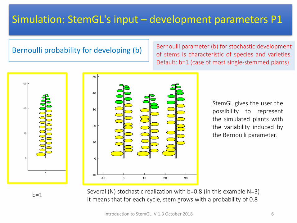
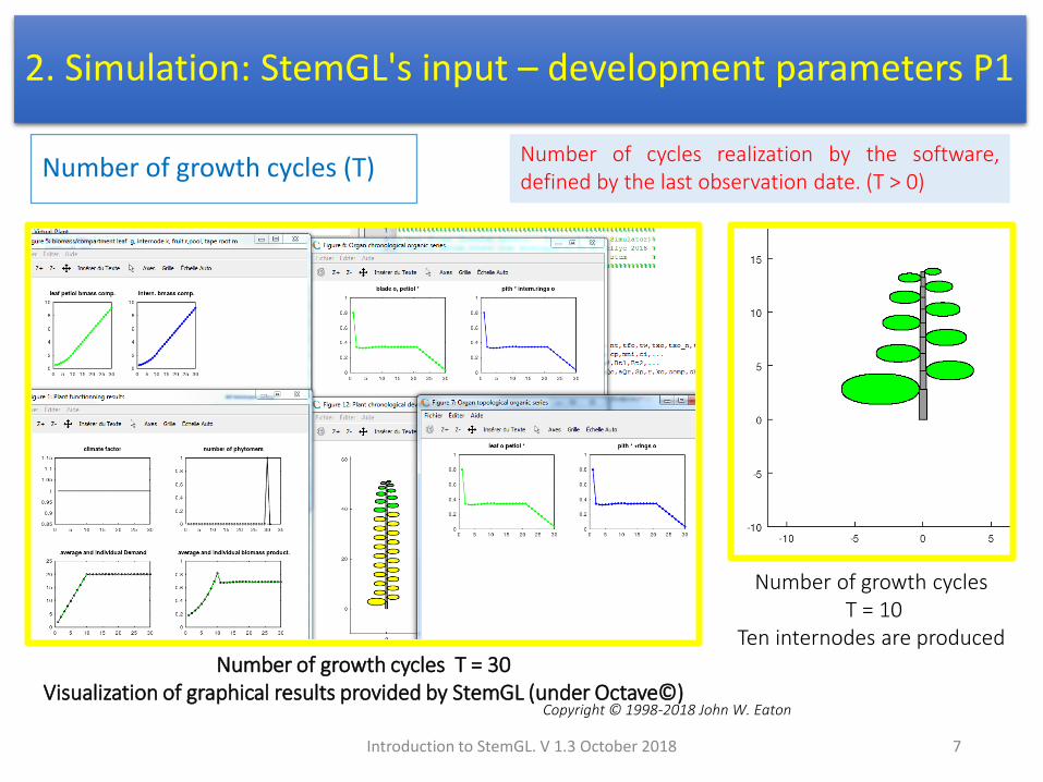
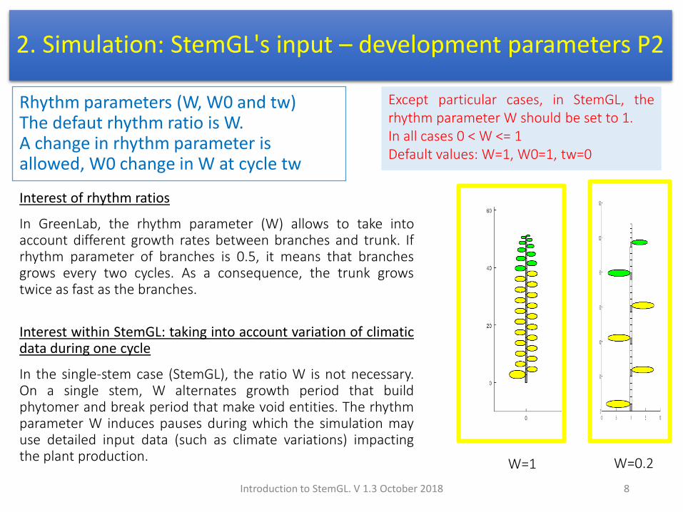
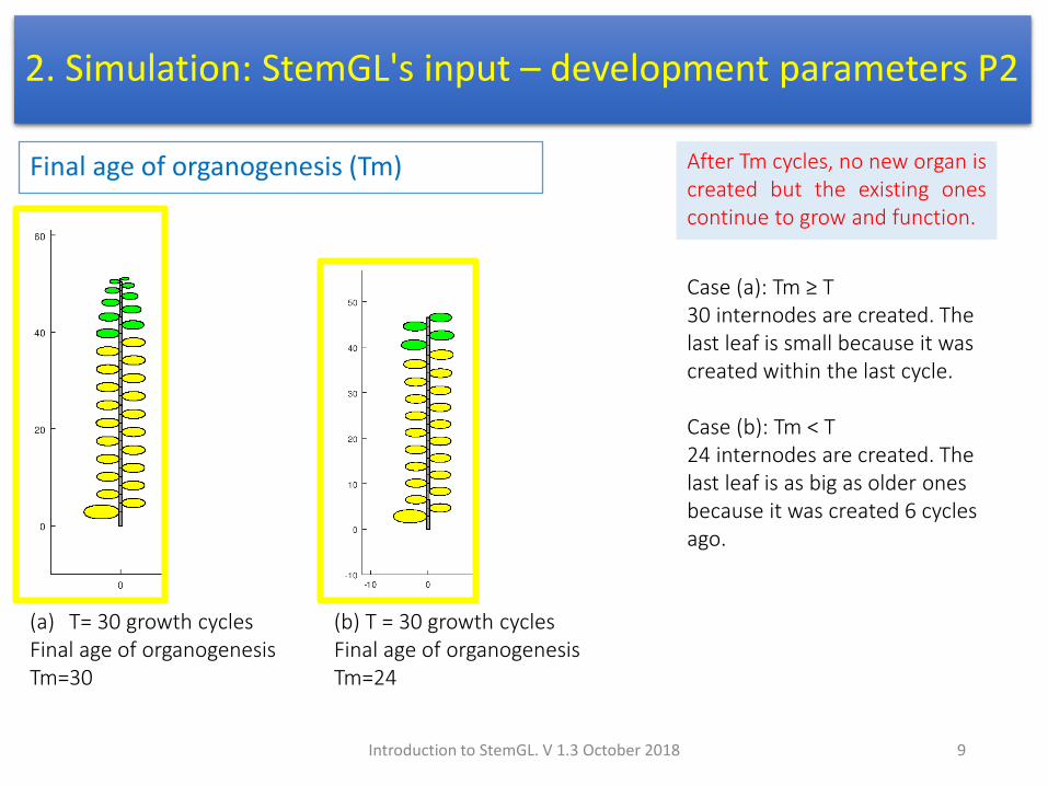
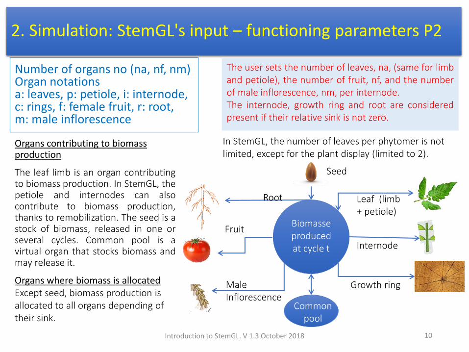
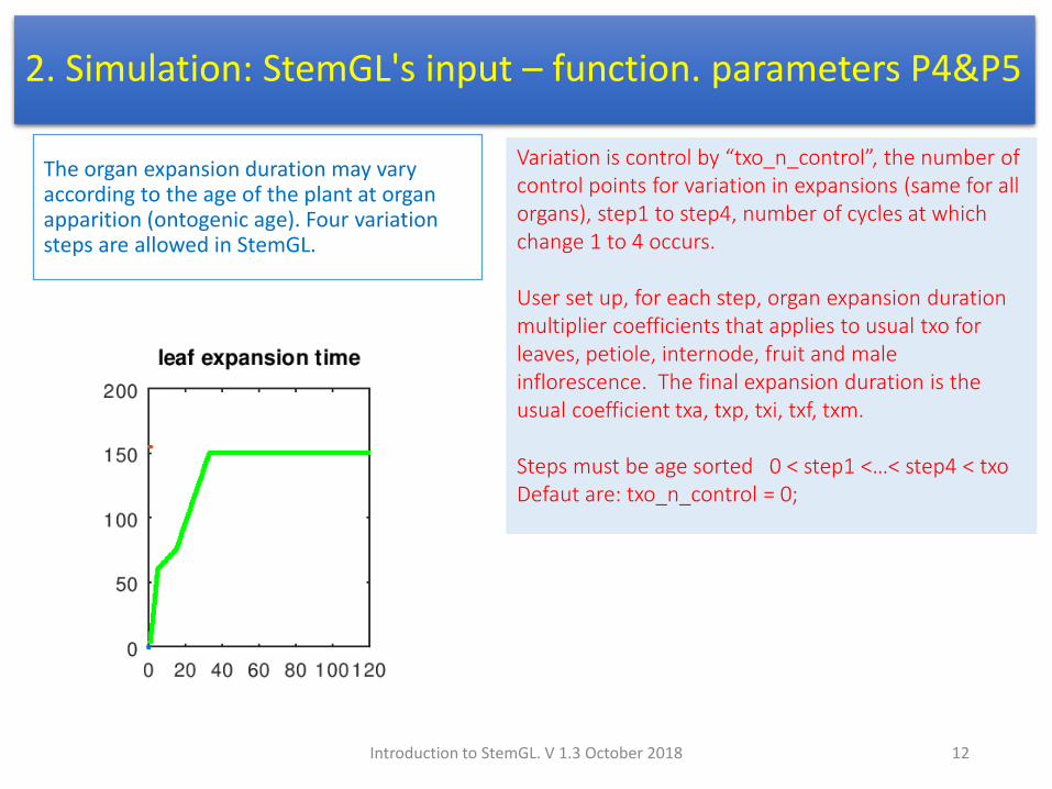
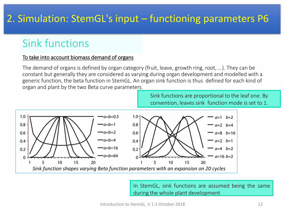
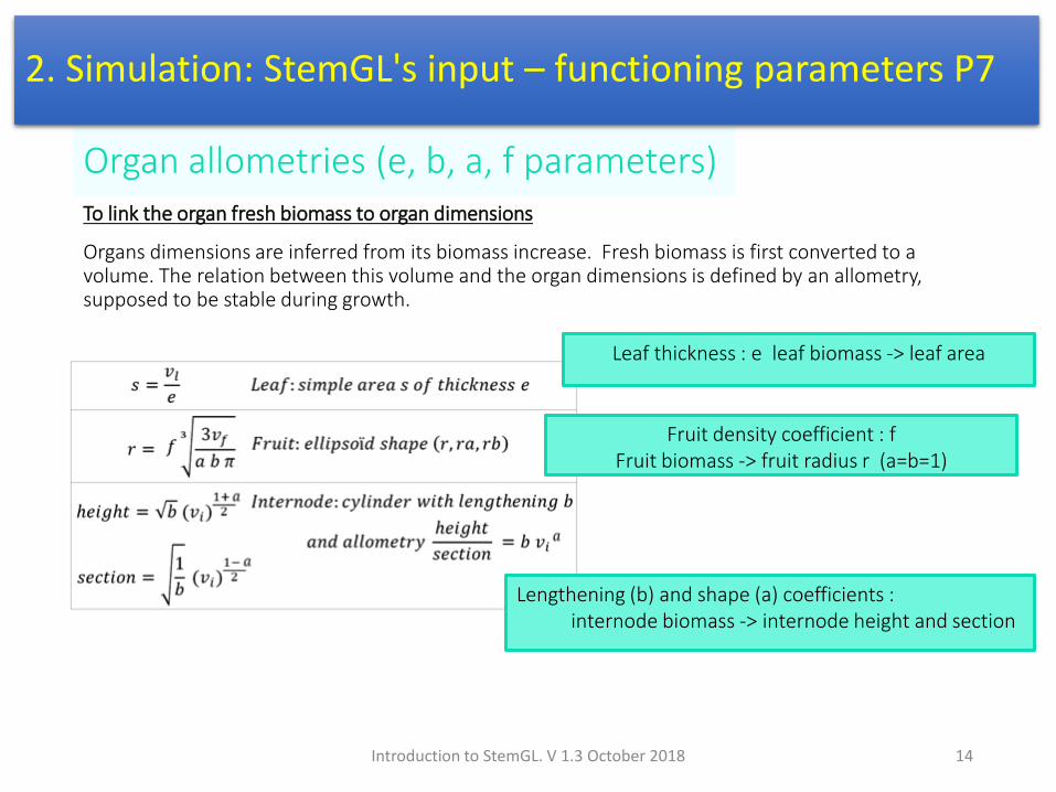
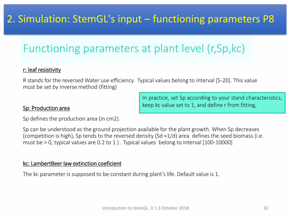
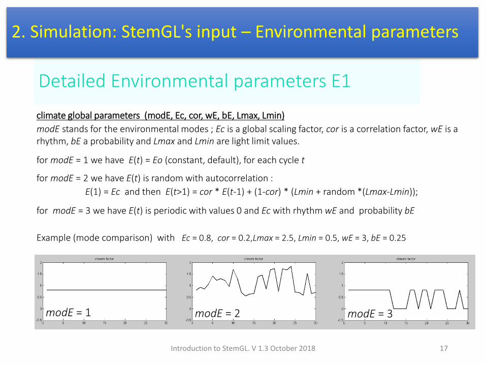
Information in the command console
During simulation
Files loaded names (parameters mask hellip) and eventually an error message (file error or data error)
At each growth cycle Cycle Biomass (cumulated increment leaf internode fruit) are given
Example (with 28 cycles) C1 Biomass0046236(0046236) leaf0015082 internode0002558 fruit0000000
helliphellip
C28 Biomass148344551(2609407942) leaf273070718 internode207233293 fruit1784252201
Computing time performances (at end of simulation for each task) Example
TOTAL CPU TIME 3984375 Total simulation 0187500
----------------------------------------------------------
Parameter loading 0031250 Development Axis 0015625
Mask load amp apply 0015625 Climate model 0000000
Organ durations 0000000 Sink Organ Beta laws 0015625
Plant Organ demand 0015625 Plant Organ growth 0109375
Organic series 0031250 Plotting results 0968750
Plant Display 0250000 Target amp Mask save 0015625
2 Simulation StemGLs output
Introduction to StemGL V 13 October 2018 19
Organ expansion and sink functions
Plant functioning results (cycle)
Climate factor number of phytomers
demand biomass production
Biomass allocated to organ componants
Organ chronological and topological series
biomass curves including those at observation times
Plant chronological and topological structure representations
Graphical diagrams (displayed at end of simulation)
2 Simulation StemGLs output Curves
Introduction to StemGL V 13 October 2018 20
Given parameters and fitted parameters
Structural development parameters
Structural parameters (development probability rhythm ratio viability hellip) must be given They can be estimated from field internode distribution statistical analysis Typically the mean variance ratio is used to estimate Bernoulli parameter b
Functional parameters to be given
The following parameters must be given Expansion and functioning times Surface of production and Organ allometries
Functional parameters to be fitted
Global functioning parameters (Qo r)
Organ sink functions (beta law parameters)
3 Fitting Principles
Introduction to StemGL V 13 October 2018 21
Data collection modes amp fitting parameters
Data collection modes (comp phyt)
Measures can be given per compartment orand per phytomer
Comp=1 stands for global organ compartment level (default 1)
Phyt=1 stands for local organ compartment level (phytomer level) (default 1)
Fitting parameters are predefined (they can be changed in the interpreted code)
The fitting method is the generalized least square method
The number of iterations is set to 10 (by default)
3 Fitting StemGLs input ndash Parameters F1
22
At least one collection mode must be active
Introduction to StemGL V 13 October 2018
Parameter selection
Selected parameters have their selector set to value 1
Unselected parameters have their selector set to value 0
Parameter that can be fitted
xQo xaQo xr xSp global functional parameters
Xpp xpi xpc xpf xpm xpt kpc kpa kpi Sink functions
xBa1 xBp1 xBi1 xBf1 xBm1 xBt1 xBa2 xBp2 xBi2 xBf2 xBm2 xBt2 Expansion Beta law parameters (two parameter per organ type)
3 Fitting StemGLs input ndash Parameters F2
23
At least one parameter selector must be active
Trick the parameter selector name is the parameter name prefixed by letter lsquoxrsquo
Example xSp is the selector of Parameter Sp
Introduction to StemGL V 13 October 2018
During simulation
Files loaded names (parameters mask hellip) and eventually an error message (file error or data error)
At each iteration the list of parameters values issued and the error The two last lines print the estimated parameter values (A) and their standard deviation (sA) Example
13047 2421442 1000 0500 25003 0700 1500 3000 3000 3000 iter = 3 error = 674794
helliphellip
12013 2221031 1024 0612 22673 0768 1738 3460 3037 3372 iter = 10 error = 151926
xr____xSp___xpp___xpe___xpf___xkpa__xkpe__xBa1__xBp1__xBi1__
A 1=1201 A 2=22210 A 3=1024 A 4=06118 A 5=2267 A 6=07682 A 7=1738 A 8=3459 A 9=3036 A 10=3371
sA 1=08969 sA 2=2261 sA 3=00539 sA 4=00479 sA 5=1671 sA 6=003414 sA 7=00967 sA 8=02151 sA 9=02132 sA 10=02456
Computing time performances (at end of simulation for each task) Example TOTAL CPU TIME 3937500 Total simulation 1687500
Parameter loading 0015625 Target loading 0062500
Development Axis 0031250 Mask load amp apply 0031250
Organ durations 0015625 Climate model 0000000
Parameter fitting 1609375 Plotting results 0765625
Parameter saving 0015625 Plant Display 0093750
3 Fitting StemGLs output Console window
Introduction to StemGL V 13 October 2018 24
Information in the command console
Graphical diagrams (displayed at end of simulation)
Fitted plant topological structure representation
Organ expansion and sink functions
Plant functioning results (cycle)
fitting overview
demand biomass production
Organ chronological and topological series
biomass curves including those at observation times
3 Fitting StemGLs output Curves
Introduction to StemGL V 13 October 2018 25
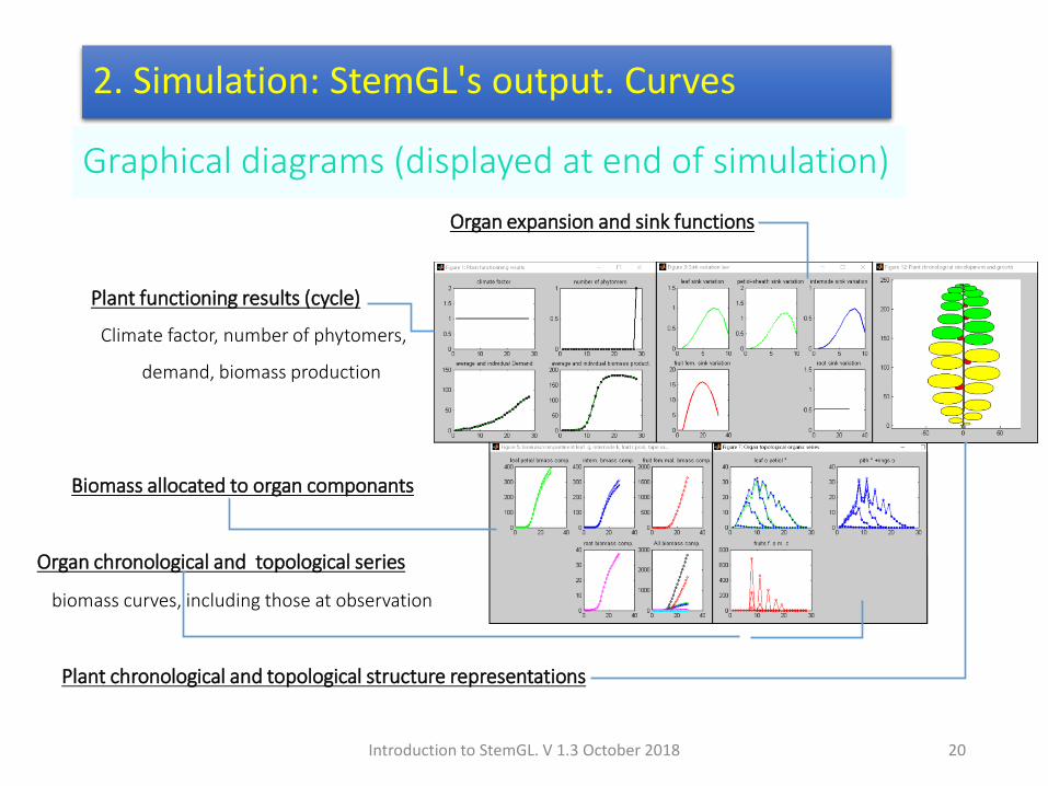
Organ expansion and sink functions
Plant functioning results (cycle)
Climate factor number of phytomers
demand biomass production
Biomass allocated to organ componants
Organ chronological and topological series
biomass curves including those at observation times
Plant chronological and topological structure representations
Graphical diagrams (displayed at end of simulation)
2 Simulation StemGLs output Curves
Introduction to StemGL V 13 October 2018 20
Given parameters and fitted parameters
Structural development parameters
Structural parameters (development probability rhythm ratio viability hellip) must be given They can be estimated from field internode distribution statistical analysis Typically the mean variance ratio is used to estimate Bernoulli parameter b
Functional parameters to be given
The following parameters must be given Expansion and functioning times Surface of production and Organ allometries
Functional parameters to be fitted
Global functioning parameters (Qo r)
Organ sink functions (beta law parameters)
3 Fitting Principles
Introduction to StemGL V 13 October 2018 21
Data collection modes amp fitting parameters
Data collection modes (comp phyt)
Measures can be given per compartment orand per phytomer
Comp=1 stands for global organ compartment level (default 1)
Phyt=1 stands for local organ compartment level (phytomer level) (default 1)
Fitting parameters are predefined (they can be changed in the interpreted code)
The fitting method is the generalized least square method
The number of iterations is set to 10 (by default)
3 Fitting StemGLs input ndash Parameters F1
22
At least one collection mode must be active
Introduction to StemGL V 13 October 2018
Parameter selection
Selected parameters have their selector set to value 1
Unselected parameters have their selector set to value 0
Parameter that can be fitted
xQo xaQo xr xSp global functional parameters
Xpp xpi xpc xpf xpm xpt kpc kpa kpi Sink functions
xBa1 xBp1 xBi1 xBf1 xBm1 xBt1 xBa2 xBp2 xBi2 xBf2 xBm2 xBt2 Expansion Beta law parameters (two parameter per organ type)
3 Fitting StemGLs input ndash Parameters F2
23
At least one parameter selector must be active
Trick the parameter selector name is the parameter name prefixed by letter lsquoxrsquo
Example xSp is the selector of Parameter Sp
Introduction to StemGL V 13 October 2018
During simulation
Files loaded names (parameters mask hellip) and eventually an error message (file error or data error)
At each iteration the list of parameters values issued and the error The two last lines print the estimated parameter values (A) and their standard deviation (sA) Example
13047 2421442 1000 0500 25003 0700 1500 3000 3000 3000 iter = 3 error = 674794
helliphellip
12013 2221031 1024 0612 22673 0768 1738 3460 3037 3372 iter = 10 error = 151926
xr____xSp___xpp___xpe___xpf___xkpa__xkpe__xBa1__xBp1__xBi1__
A 1=1201 A 2=22210 A 3=1024 A 4=06118 A 5=2267 A 6=07682 A 7=1738 A 8=3459 A 9=3036 A 10=3371
sA 1=08969 sA 2=2261 sA 3=00539 sA 4=00479 sA 5=1671 sA 6=003414 sA 7=00967 sA 8=02151 sA 9=02132 sA 10=02456
Computing time performances (at end of simulation for each task) Example TOTAL CPU TIME 3937500 Total simulation 1687500
Parameter loading 0015625 Target loading 0062500
Development Axis 0031250 Mask load amp apply 0031250
Organ durations 0015625 Climate model 0000000
Parameter fitting 1609375 Plotting results 0765625
Parameter saving 0015625 Plant Display 0093750
3 Fitting StemGLs output Console window
Introduction to StemGL V 13 October 2018 24
Information in the command console
Graphical diagrams (displayed at end of simulation)
Fitted plant topological structure representation
Organ expansion and sink functions
Plant functioning results (cycle)
fitting overview
demand biomass production
Organ chronological and topological series
biomass curves including those at observation times
3 Fitting StemGLs output Curves
Introduction to StemGL V 13 October 2018 25
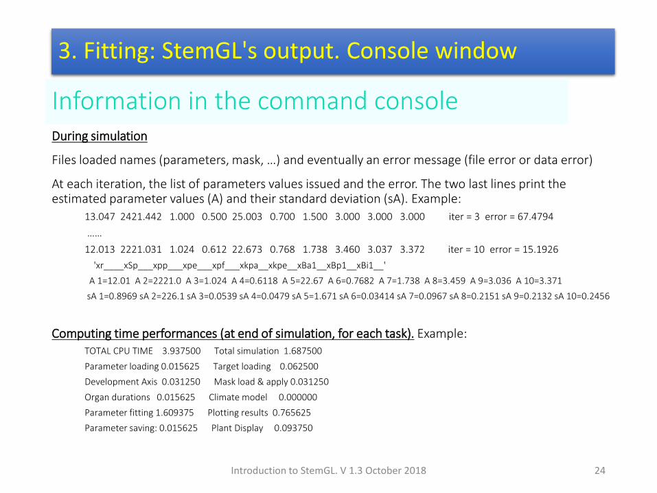
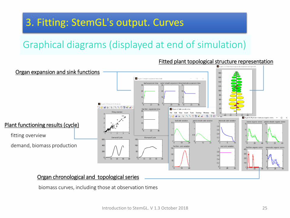