Embed Size (px)
Citation preview
Steam System Heat Exchanger Network Optimisation
Using Degenerate Solutions: A focus on Pressure Drop
and Boiler Efficiency
by
Tim Price
A dissertation submitted in partial fulfilment of the requirements for the degree
PhD: Chemical Engineering
in the
Faculty of Engineering, the Built Environment and Information Technology
Supervisor: Prof. T. Majozi
University of Pretoria
February 2016
© University of Pretoria
i
Synopsis
This work presents a revised methodology to minimise pressure drop through a
steam system heat exchanger network (HEN). This is based on previous work
where network pressure drop is minimised after utility flow through the network
has been reduced to its minimum. With the minimum utility flow as a
parameter, the proposed methodology enlarges the solution space of the
problem in an attempt to find a better pressure drop solution. The resulting
minimum pressure drop found using this method is an improvement of 1.1 %
and 7.4%, in two case studies respectively, on the current HEN minimisation
problem formulation. The method is then extended to maintain boiler
efficiency with the same minimum steam flowrate. Due to the simpler nature of
the problem of maintaining boiler efficiency the proposed methodology did
not yield improvements to the steam flowrate however a wider variety of
network configurations was found.
The steam flowrate to a HEN can be substantially reduced with the application
of process integration. Reducing the steam flowrate to the HEN involves
creating series heat exchanger connections, which ultimately increase the
pressure drop to the system. The reduced steam flowrate also compromises the
return condensate temperature and consequently reduces the efficiency of
the steam boiler.
A HEN optimisation and design methodology exists whereby the minimum
steam flowrate to a heating utility system can be found and the pressure drop
through the HEN can be minimised. This methodology does not however
incorporate the full solution space of potential network configurations. This is as
a result of network conditions of optimality which fix the outlet temperature of
condensate streams leaving heat exchangers in order to achieve a globally
optimal minimum steam flowrate.
The minimum steam flowrate can still be achieved by relaxing the optimality
conditions and allowing for variable heat exchanger outlet temperatures.
Solutions of this nature are referred to as degenerate and are formulated with
bilinear terms forming part of the energy balance constraints. The presence of
© University of Pretoria
ii
bilinear terms results in a nonlinear, nonconvex mixed integer nonlinear
programming (MINLP) problem. The bilinear terms are catered for in the
methodology by the reformulation and linearisation technique of Quesada
and Grossmann (1995) as well as the transformation and convexification
technique of Pörn et al (2008). The reformulation and linearisation approach
proved to be the most successful for the proposed problem.
By utilising the larger solution space created by incorporating degenerate
solutions into the HEN design process, many HEN design variables can
potentially be further optimised once a minimum steam flowrate has been
achieved.
Consequently, this thesis concerns the optimisation of a steam system HEN by
finding the minimum steam flowrate to the system and using it as a parameter
while relaxing the conditions of network optimality to create solutions which
can be degenerate. The complexities of MINLPs in the degenerate solutions
are explored and a methodology to further optimise network pressure drop
through heating networks is proposed. The methodology was also used to
maintain boiler efficiency with a reduced steam flowrate which was achieved,
but not improved upon from previous methodologies.
While this methodology does not guarantee an improved HEN pressure drop,
solutions adhering to the conditions of network optimality also fall within the
solution space of the proposed methodology, therefore solutions achieved
with current techniques from literature will not be compromised.
© University of Pretoria

Declaration
I, Tim Price, with student number 04359968, declare that:
1. I understand what plagiarism entails and am aware of the University of
Pretoria’s policy in this regard.
2. I declare that this dissertation is my own, original work. Where someone
else’s work was used (whether from a printed source, the internet or any
other source) due acknowledgement was given and reference was
made according to departmental requirements.
3. I did not make use of another student’s previous work and submit it as
my own.
4. I did not allow and will not allow anyone to copy my work with the
intention of presenting it as his or her own work.
5. The work presented in this dissertation has not been submitted anywhere
else in partial or full fulfilment of another degree.
Signature __________________
© University of Pretoria

Acknowledgements
Firstly I would like to thank my supervisor, Prof Thoko Majozi, for his support,
encouragement and patience. My time spent under his guidance has been an
extremely rewarding and I have certainly learnt a lot.
I would also like to acknowledge my friends in the process integration group,
Jane, Sheldon, Esmael, Bongani, and Yvette.
I would like to thank my friends at ERM who have been very supportive and
encouraging as well as understanding about the time constraints involved in
my university work. Thank you Gary, Peter, Bianca, Laura, Charlotte, Sean,
Baptiste, Dylan, Dave and Lisa.
A special thanks to my parents for their love and support. I truly could not have
accomplished this without them. Also to my uncle and granddad, thank you
very much! Then to my friends off campus, my housemate Steve, thank you for
a few super years, I really enjoyed the talks in the kitchen. To Shaun, Des,
Brendan, Melana, Stacey, Ricky, Binny, Laura, Net, El, Kyra, Max and Luci thank
you for everything. To Ally, I have had the most incredible time with you, thank
you for all of your kindness, help, encouragement and a lot of fun completing
my thesis. You truly are the best!
Finally, I would like to acknowledge the financial support of Environmental
Resources Management.
© University of Pretoria
Contents
1. Introduction ............................................................................................................. 1
1.1. Background ...................................................................................................... 1
1.2. Basis and Objectives ....................................................................................... 2
1.2.1. Problem Statement .................................................................................. 3
1.3. Thesis Scope ..................................................................................................... 4
1.4. Thesis Layout ..................................................................................................... 4
1.5. References ....................................................................................................... 5
2. Literature Review .................................................................................................... 7
2.1. HEN Optimisation ............................................................................................. 7
2.1.1. Early HEN Synthesis, Design and Optimisation ..................................... 7
2.1.2. Other Applications of Pinch Analysis ..................................................... 9
2.1.3. Early Mathematical Programming ........................................................ 9
2.2. Water Utility Optimisation ............................................................................. 10
2.2.1. Wastewater Optimisation ..................................................................... 10
2.2.2. Cooling Water System Optimisation .................................................... 12
2.2.3. Network Pressure Drop .......................................................................... 15
2.3. Heating Utility Optimisation .......................................................................... 19
2.3.1. Boiler Efficiency....................................................................................... 24
2.3.2. HEN Pressure Drop .................................................................................. 28
2.4. Conditions of Network Optimality ............................................................... 30
2.5. Some Mathematical Techniques for Nonlinear, Nonconvex Constraints
32
2.5.1. Relaxation and Linearisation ................................................................ 33
2.5.2. Transformation and Convexification ................................................... 34
2.5.3. Notes on MINLP Solvers .......................................................................... 39
© University of Pretoria
2.6. Conclusion ...................................................................................................... 41
2.7. References ..................................................................................................... 42
3. Motivation for Study ............................................................................................. 50
3.1. Background .................................................................................................... 50
3.1.1. Previous Work .......................................................................................... 50
3.1.2. Modelling Experience ............................................................................ 51
3.2. System of Interest ........................................................................................... 52
3.3. HEN Pressure Drop ......................................................................................... 54
3.3.1. Background to HEN Pressure Drop ...................................................... 54
3.3.2. Steam System HEN Pressure Drop Problem ........................................ 61
3.4. Boiler Efficiency .............................................................................................. 62
3.4.1. Derivation ................................................................................................ 62
3.4.2. Sensitivity.................................................................................................. 64
3.5. Optimality of Flow Solutions in Network Optimisation Problems ............. 68
3.5.1. Degenerate Solutions ............................................................................ 69
3.6. Branch and Bound MINLP Solvers ............................................................... 70
3.6.1. Techniques to Overcome Bilinear Terms and Nonconvexity ........... 73
3.6.2. Application in Degenerate Flow Network Problems ......................... 75
3.6.3. Solution Process ...................................................................................... 76
3.7. References ..................................................................................................... 76
4. Model Formulation ................................................................................................ 81
4.1. Flow Minimisation Constraints ...................................................................... 81
4.1.1. Steam System Heat Exchanger Network Flow Minimisation
Constraints ............................................................................................................. 81
4.1.2. Conditions of Flow Optimality .............................................................. 89
4.2. Pressure Drop Minimisation Constraints ...................................................... 89
4.2.1. Steam System Heat Exchanger Network Pressure Minimisation
Constraints ............................................................................................................. 90
© University of Pretoria
4.2.2. Pressure Drop Correlations .................................................................... 99
4.3. Basic Steam System Pressure Drop Minimisation Model ........................ 102
4.3.1. Combination of Basic Constraints ..................................................... 102
4.3.2. Problem Formulation............................................................................ 103
4.3.3. Singularities ............................................................................................ 104
4.3.4. Pressure Drop Approximation ............................................................. 105
4.3.5. Piecewise Approximation with MINLP Solvers .................................. 109
4.4. Degenerate Solutions ................................................................................. 111
4.4.1. Temperature and Flow Limits .............................................................. 111
4.5. Relaxation and Linearisation ..................................................................... 113
4.5.1. Sensible Energy Constraint with Relaxation and Linearisation
Technique ............................................................................................................ 114
4.5.2. Initial MILP Problem .............................................................................. 115
4.5.3. Exact Problem ...................................................................................... 117
4.5.4. Solution Strategy for Relaxation and Linearisation Formulation .... 118
4.6. Transformation and Convexification ........................................................ 122
4.6.1. Exponential Transform ......................................................................... 123
4.6.2. Potential Transform .............................................................................. 124
4.6.3. Sensible Energy Constraint with Transformation and
Convexification ................................................................................................... 125
4.6.4. Approximation of Nonlinear ET and PT Terms ................................... 126
4.6.5. Tangential Piecewise Linear Approximation .................................... 132
4.6.6. Tangential Piecewise Linear Approximation using Branch and
Bound MINLP Algorithms .................................................................................... 137
4.6.7. Pressure Drop Constraints in the Transformation and
Convexification Formulation ............................................................................. 142
4.6.8. Additional Model Considerations ...................................................... 143
© University of Pretoria
4.6.9. Solution strategy for Transformation and Convexification
Formulation .......................................................................................................... 146
4.7. Additional Solver Techniques .................................................................... 149
4.8. Consideration for Steam System Boiler Efficiency ................................... 150
4.8.1. Calculation of Boiler Efficiency .......................................................... 151
4.8.2. Sensitivity of Boiler Efficiency .............................................................. 154
4.8.3. Dedicated Pre heater to Maintain Boiler Efficiency ....................... 155
4.8.4. Solution Strategy................................................................................... 160
4.9. Summary ....................................................................................................... 162
4.10. References ................................................................................................ 164
5. Case Studies ........................................................................................................ 166
5.1. Case Study HEN ........................................................................................... 166
5.2. System Pressure Drop with Fixed Outlet Temperature ............................ 168
5.2.1. Solution from Price and Majozi (2010c) ............................................. 169
5.2.2. Solution with Exact Minimum Steam Flowrate ................................. 170
5.2.3. Reworked Formulations ....................................................................... 171
5.2.4. Solution .................................................................................................. 171
5.2.5. Discussion of Results ............................................................................. 173
5.3. Degenerate Solution Pressure Drop with Relaxation and Linearisation
Formulation .............................................................................................................. 174
5.4. Degenerate Solution Pressure Drop with Transformation and
Convexification Formulation ................................................................................. 178
5.4.1. Modelling Experience .......................................................................... 178
5.4.2. Problem solution ................................................................................... 180
5.5. Comparison of Results ................................................................................ 185
5.5.1. Relaxation and Linearisation Result ................................................... 185
5.5.2. Transformation and Convexification Result ...................................... 186
5.5.3. Conclusion ............................................................................................ 186
© University of Pretoria
5.6. Second Case Study HEN ............................................................................ 187
5.6.1. Minimum Steam Flowrate ................................................................... 188
5.6.2. System Pressure Drop ........................................................................... 189
5.6.3. Discussion of Results ............................................................................. 192
5.7. Maintaining Boiler Efficiency ...................................................................... 192
5.7.1. Solution from Price and Majozi (2010a) ............................................ 195
5.7.2. Degenerate Solution with Relaxation and Linearisation Formulation
197
5.7.3. Degenerate Solution with Transformation and Convexification
Formulation .......................................................................................................... 202
5.7.4. Comparison of Results ......................................................................... 205
5.8. References ................................................................................................... 206
6. Conclusions and Discussion ............................................................................... 208
6.1. Conclusions .................................................................................................. 208
6.1.1. Pressure Drop Comparison ................................................................. 208
6.1.2. Boiler Efficiency Comparison .............................................................. 210
6.2. Discussion ...................................................................................................... 211
6.3. References ................................................................................................... 213
Appendix A. ................................................................................................................ 214
A.1. Heat Exchanger Guidelines ....................................................................... 214
A.2. Piping Guidelines ......................................................................................... 217
A.3. References ................................................................................................... 217
Appendix B. ................................................................................................................. 218
B.1. Relaxation Linearisation Technique Described by Quesada and
Grossmann (1995) ................................................................................................... 218
B.2. Glover (1975) Transformation ..................................................................... 220
B.3. References ................................................................................................... 221
© University of Pretoria
Chapter 1 Introduction
1
1. Introduction
The optimisation of utility systems is beneficial to both grassroots process designs as
well as existing processes. Lower utility consumption reduces costs through energy
consumption, environmental impact and can have process benefits such as
removing bottlenecks to expansion. Two key utilities in process plants are steam and
cooling water. The reduction in the consumption of either of these has been shown
to greatly reduce operational costs or capital costs for grassroots design. Reuse and
recycle is very effective at reducing the consumption of fresh utilities in process
networks. The key to reuse networks is to allow series heat exchanger connections as
opposed to traditional parallel network designs. This is effectively shown for cooling
systems by Kim and Smith (2001) and for heating systems by Coetzee and Majozi
(2008).
These processes do however become more complex as the utility flows are reduced
and care must be taken to ensure that the systems are not adversely affected by
such reductions. The consideration of holistic systems has been shown to yield great
utility flow savings while not adversely affecting other factors of heating and cooling
circuits such as the steam boiler or cooling towers. Focus can now be directed to
other design variables in the heat exchanger networks (HENs) themselves.
This chapter discusses the background, objectives, scope and layout of this thesis.
1.1. Background
Reuse and recycle of a heating or cooling utility involves using the utility stream
leaving a heat exchanger to further heat or cool an additional process stream. This
series type connection has been proposed to reduce utility consumption when used
in place of traditional parallel networks which see the utility return to its source
directly, typically a steam boiler or cooling tower. This has been accomplished
successfully for cooling systems by Kim and Smith (2001) and for heating systems by
Coetzee and Majozi (2008).
© University of Pretoria
Chapter 1 Introduction
2
A consequence of series connections is a greater pressure drop of the utility flow
through the network. Increased pressure drop could lead to the requirement of
additional fluid movers in retrofit designs and additional capital expenditure in
grassroots designs. Reusing process utilities can also have adverse effects on the
utility source, namely cooling towers and steam boilers. In this work steam systems
are investigated. Reusing hot process utilities also reduces steam condensate return
temperature to the steam boiler which can adversely affect the boiler efficiency.
Pressure drop and boiler efficiency have thus been incorporated into many HEN
design philosophies.
A condition of network optimality developed by Savelski and Bagajewicz (2001)
exists which can guarantee a minimum utility flowrate. An infinite number of network
layouts can achieve the optimality conditions of Savelski and Bagajewicz (2001).
Therefore it is possible to optimise additional design aspects of the network. This
concept was used to optimise pressure drop in HENs for cooling system by Kim and
Smith (2003) as well as Gololo and Majozi (2013) and in heating systems by Price and
Majozi (2010c).
A minimum utility flow can however also be achieved without all of the conditions of
network optimality being adhered to. Savelski and Bagajewicz (2001) refer to such
solutions as degenerate and utilise these to optimise internal network features such
as the number of connections. The authors first use the conditions of optimality to
target for the minimum utility flowrate and then optimise the network structure in a
manual and iterative procedure. In heating systems, by allowing for degenerate
solutions the utility stream temperature leaving heat exchangers becomes a
variable and creates bilinear terms with the mass flowrate of steam in the energy
balance constraints. These bilinear terms cause difficulty for MINLP solvers as they are
both nonlinear and nonconvex.
1.2. Basis and Objectives
By relaxing the optimality condition of Savelski and Bagajewicz (2001) additional flow
and network arrangement opportunities can be found. HEN arrangements of this
type are referred to as degenerate solutions. These arrangements may give greater
© University of Pretoria
Chapter 1 Introduction
3
flexibility to the steam HEN arrangements so as to find an improved minimum
pressure drop as well as result in better steam system alterations to maintain boiler
efficiency while still achieving the minimum steam flowrate of the system.
MINLP solvers are adept at handling complex problems, however nonconvex terms
can cause difficulties. A number of techniques in literature have attempted to aid
the solution of MINLP problems. Quesada and Grossmann (1995) utilise a technique
of relaxation and linearisation to overcome bilinear terms. This technique was also
adopted by Price and Majozi (2010a). Pörn et al. (2008) describe transformation
techniques to transform nonconvex terms in model formulations into convex terms.
The network pressure drop minimisation model can be formulated with nonlinear
pressure drop terms, however the inclusion of degenerate solutions creates bilinear
terms. The bilinear terms are nonconvex and will be treated with appropriate
techniques.
Degenerate solutions directly affect the HEN and therefore the focus of this work is
on finding an improved steam system HEN pressure drop with the inclusion of
degenerate solutions. This work attempts to formalise an approach to utilising
degenerate solutions in HEN optimisation while also closing the loop on the steam
system HEN pressure drop work initiated by Price and Majozi (2010c). Degenerate
solutions are also incorporated into the boiler efficiency optimisation problem with
retrofit steam flowrate minimisation.
1.2.1. Problem Statement
The steam flowrate to a steam system HEN can be minimised by the reuse and
recycle of hot condensate to provide additional heat to process streams. Reuse and
recycle requires series connections in the HEN. A consequence of these series
connections is an increase in the utility pressure drop through the HEN. Another
consequence of the reuse and recycle of hot condensate is the lowering of the
boiler condensate return temperature. This, in addition to the reduced flowrate, can
have detrimental effects on the steam boiler efficiency.
A means to guarantee a minimum steam flowrate is to implement the network
condition of optimality which involves fixing utility stream heat exchanger outlet
© University of Pretoria
Chapter 1 Introduction
4
temperatures to their lower limits which reduces the solution space of feasible HEN
layouts.
The problem statement can, therefore, be formally stated as follows,
Given:
a steam system comprising a set of heat exchangers linked to a boiler with
limiting temperatures and fixed duties; and
a predetermined minimum steam flowrate for the HEN
determine the minimum network pressure drop while relaxing the network condition
of optimality used to find the minimum steam flowrate for the system while
maintaining the minimum steam flowrate. In addition determine whether the steam
boiler efficiency can be maintained in an improved manner.
1.3. Thesis Scope
The scope of this research is to investigate the effects of relaxing the conditions of
network optimality on HEN pressure drop as well as maintaining boiler efficiency
while still achieving a minimised steam flowrate for the system.
Relaxing the conditions of network optimality involves allowing the outlet
temperatures of utility streams leaving heat exchangers to vary.
A mathematical programming approach is proposed to solve the HEN pressure drop
minimisation problem using degenerate solutions. The mathematical techniques
created to incorporate degenerate solutions into the HEN are then applied to
maintain the boiler efficiency with a dedicated heat exchanger with variable duty
after retrofit steam flowrate minimisation.
1.4. Thesis Layout
This thesis is divided into the following chapters:
© University of Pretoria
Chapter 1 Introduction
5
Chapter 1 introduces the thesis and provides relevant background to the
work. The objectives and scope of the work are presented and a description
of the thesis layout also given;
Chapter 2 provides a literature review of research in the fields of HEN
optimisation, wastewater, cooling water and steam utility optimisation as well
as techniques from literature to aid the solution of MINLP problems;
Chapter 3 shows a motivation for the study. Here previous work is
deconstructed and a basis for the consideration of degenerate solutions for
HEN pressure drop minimisation as well as boiler efficiency is given. The
solution of MINLP problems is also discussed;
Chapter 4 includes the formal model formulation. Flow minimisation
constraints are provided as well as network pressure drop constraints. Solution
techniques to aid the solution of problems with bilinear terms are introduced
and adapted for the HEN pressure drop minimisation model. The chapter is
concluded by incorporating the steam system alterations and constraints
required to maintain the boiler efficiency with a reduced steam flowrate;
Chapter 5 provides a case study where the original steam system pressure
drop minimisation model of Price and Majozi (2010c) is given and solved using
the techniques described in the thesis. The optimal pressure drop minimisation
layout using degenerate solutions is also provided and the solution is
compared to the results of the Price and Majozi (2010c) model. Similarly, the
case study presented by Price and Majozi (2010a) is utilised with the
allowance for degenerate solutions and this is then compared to the boiler
efficiency problem of Price and Majozi (2010a); and
Chapter 6 discusses conclusions of the work and evaluates the success of the
methods described. A discussion of the results and suggestions for areas of
further research and improvement conclude the chapter.
1.5. References
Coetzee, W.A. and Majozi, T. (2008) Steam System Network Design Using Process
Integration, Ind. Eng. Chem. Res 2008, 47, 4405-4413.
© University of Pretoria
Chapter 1 Introduction
6
Gololo, K. V. and Majozi, T. (2013) Complex Cooling Water Systems Optimization with
Pressure Drop Consideration, Ind. Eng. Chem. Res 2013, 52, 7056−7065.
Kim, J. K. and Smith, R. (2001) Cooling water system design, Chemical Engineering
Science, Vol 56, pages 3641-3658.
Kim, J. K. and Smith, R. (2003) Automated retrofit design of cooling-water systems,
Process Systems Engineering, Vol 49, No7, pages 1712-1730.
Price, T. and Majozi, T. (2010a). On Synthesis and Optimization of Steam System
Networks. 1. Sustained Boiler Efficiency. Industrial Engineering Chemistry Research 49
, 9143–9153.
Price, T. and Majozi, T. (2010c). On Synthesis and Optimization of Steam System
Networks. 3. Pressure Drop Consideration. Industrial Engineering Chemistry Research
49 , 9165–9174.
Pörn, R. Björk, K. and Westerlund, T. (2008). Global solution of optimization problems
with signomial parts. Discrete Optimization 5 , 108-120.
Quesada, I. and Grossmann, I. E. (1995) Global optimisation of bilinear process
networks with multi component flows, Computers and Chemical Engineering 19, No
12, pages 1219-1242.
Savelski, M. J. and Bagajewicz, M. J. (2001), On the Use of Linear Models for the
Design of Water Utilization Systems in Process Plants with a Single Contaminant,
Institution of Chemical Engineers, Trans IChemE 2001 , 79, Part A, 600-610.
© University of Pretoria
Chapter 2 Literature Review
7
2. Literature Review
This section is intended to discuss the relevant literature in various areas related to
this field of research. These areas include heat exchanger network optimisation,
heat exchanger network pressure drop optimization, MINLP solvers, as well as model
manipulations which further improve their performance.
2.1. HEN Optimisation
The HEN of a process is intended to provide heating and cooling to process streams.
In a process where there are both hot and cold streams, there exists an opportunity
to exchange heat between the process streams themselves and reduce the
amount of utilities that would ordinarily have been used to heat or cool the relevant
process streams. In the context of this work, the reduction of utilities using
improvements to the arrangement of the HEN will be referred to as HEN optimisation.
Improvements to other aspects of HEN design can also lead to reduced costs, such
as area optimisation and improved heat exchanger design. These are, however,
capital expenses that can often be overshadowed by operating expenses, such as
utilities, in the life of a plant. This, coupled with the tendency for utility prices to
increase, makes utility reduction and the study of HEN optimisation of paramount
importance in process plant design.
Arguably the most common hot and cold utilities in process plants are steam and
cooling water, respectively. The utility consumption can be reduced by process
changes or improvements, but also HEN optimisation. Improvements can be made
to maximize the amount of process to process heat exchange, or maximize the
efficiency at which the utilities are used.
2.1.1. Early HEN Synthesis, Design and Optimisation
Several concepts have been developed to aid in the field of HEN optimisation. A
prominent concept is pinch analysis which can be used to find the minimum utility
requirement of a process. Pinch analysis can be carried out using graphical
© University of Pretoria

Chapter 2 Literature Review
8
techniques, which can give a designer insight into the process and its constraints.
Mathematical programming techniques are also prevalent in literature. While these
appear as a more black box approach, the extent of application of mathematical
programming makes it an excellent approach to HEN synthesis, design and
optimisation.
Graphical techniques were first utilised by Hohmann (1971), who optimised a trade
off between utilities and heat exchange area. This work laid the foundation for the
formation of the Temperature-Duty (T-Q) diagram of Huang and Elshout (1976),
which is used to represent process heating and cooling utility requirements in the
form of a composite curve. The utilities can also be represented on the T-Q diagram
and can be used to find the pinch point in the system, as shown by Umeda, Handa
and Shiroko (1979). The pinch point is denoted where the process composite curve
meets the utility supply curve. This technique was successfully used to target for a
minimum utility flowrate.
Alternatively, Linnhoff and Flower (1978) developed the Problem Table Algorithm to
both target minimum utilities and help design HENs. The results of this systematic
technique were then used by the authors to construct a further graphical aid, the
Grand Composite Curve. Whereas the T-Q diagram allowed a single utility to be
targeted, the grand composite curve combines hot and cold utilities to target the
minimum utility usage for the system.
Early work on HEN design by Linnhoff et al. (1979) showed how complicated this
process was. This work led to a comprehensive understanding and subsequent
design philosophy for HENs presented by Linnhoff and Hindmarsh (1982). This design
methodology focussed on the pinch principle and has been the cornerstone in HEN
design.
Asante and Zhu (1997) optimized HEN retrofit designs by not only considering the
maximization of heat recovery with promising topological matches but also the
minimisation of cost of additional heat exchange area. The complexities of HENs
and the effect of network layout and topography is illustrated while an automated
and interactive method utilising practical engineering is proposed to optimise the
© University of Pretoria

Chapter 2 Literature Review
9
design. This work laid the foundation for further network optimisation where layout
and topography were taken into account.
2.1.2. Other Applications of Pinch Analysis
Other utility systems also stand to benefit from pinch technology. Most common of
these is arguably mass transfer in wastewater treatment. Other mass transfer
applications are the likes of hydrogen pinch and water pinch in certain processes.
Mass transfer, like heat transfer, relies on a driving force. Much work has been done
in understanding and utilising concentration driving forces in mass transfer, while
similarly temperature serves as the key driving force in heat transfer. Key research in
both fields will be discussed in later chapters.
2.1.3. Early Mathematical Programming
Papoulias and Grossmann (1983a, 1983b and 1983c) set about to create a more
systematic plant design methodology than the simple thermodynamic and heuristic
techniques commonly used at the time. This method utilised Mixed Integer Linear
Programming (MILP) models of plants at various discrete operating conditions, which
required large amounts of background work. This work did, however, show the
flexibility of mathematical programming in plant design and the importance of fully
understanding the bounds of the optimisation problem.
The authors were able to explore many different arrangements of the systems
through an effective and comprehensive superstructure. This superstructure was
largely designed using thermodynamic and heuristic techniques. The power of the
mathematical programming approach is then to find the optimal arrangement
which is sometimes not obvious for even simple systems.
Early work in process to process HEN optimisation and mathematical programming
laid a platform to further optimise the utility systems. The following sections examine
optimisation of both cooling and heating systems.
© University of Pretoria
Chapter 2 Literature Review
10
2.2. Water Utility Optimisation
As described in Section 2.1.2, similarity exists in heat and mass transfer in that a
driving force is needed to transfer energy or material from streams of a high
temperature or concentration to those with a low temperature or concentration. In
process plants water is used as a key medium for both. Cooling systems frequently
employ cooling water circuits to provide a cooling utility for hot process streams
while cleaning water can be used to remove contaminants and unwanted material
from process vessels. This section discusses certain key areas of research in
wastewater and cooling water system optimisation.
2.2.1. Wastewater Optimisation
Takama et al. (1980) present the water allocation problem (WAP) for petroleum
refineries. These authors utilise the concepts of the reuse and regeneration of
wastewater within process wastewater circuits by generating a superstructure of all
possible connections and then eliminating features which are not economic.
El-Halwagi and Manousiouthakis (1989) expanded the pinch design method based
on that of heat exchangers developed by Linnhoff and Hindmarsh (1982) for mass
exchange networks. They created a more general approach for mass exchange
between streams of high and low concentration. The approach was only applicable
to simple systems due to the heuristic nature of the design method, however El-
Halwagi and Manousiouthakis (1990) developed a simple mathematical
programming approach which overcomes this design shortfall.
Wang and Smith (1994) presented a conceptual approach to the WAP. The authors
allowed for individual process constraints to be considered by defining the minimum
and maximum contaminant concentrations for the limiting water profile. These
profiles for various streams could then be combined into a limiting composite curve
where minimum targets could be set. Targets were initially set to maximise reuse
while regeneration was also considered. With a minimum wastewater target set the
authors designed the network according to two methods with differing objectives
while still achieving the target set in the initial phase. They subdivided the limiting
composite curve into mass load intervals and utilised the network design grid
diagram of Linnhoff and Flower (1978) to complete the design.
© University of Pretoria
Chapter 2 Literature Review
11
This procedure was thorough and allowed many network and process aspects to be
considered, however it was also time consuming. Alternatively, mathematical
solutions to network design were considered complex. Olesen and Polley (1996)
identified the complexities of the design procedure proposed by Wang and Smith
(1994) and proposed a much simplified procedure for single contaminants. Due to
the inspection type solution procedure, this process was found to be restricted to
smaller numbers of operations.
The complications involving numerical techniques, or mathematical programming,
were found to be primarily due to the nonlinear nature of problems containing
bilinear terms, which lead to infeasible solutions with conventional mathematical
solvers at the time. Doyle and Smith (1997) proposed an iterative procedure to
account for the bilinearity, while Alva-Argaez et al. (1998) attempted a two phase
solution procedure for their MINLP version of the problem. Huang et al. (1999) also
presented a mathematical programming solution for the problem of water
allocation as well as treatment. The work of the authors listed above showed a gap
in the water allocation problem, where network design was concerned. The time
consuming nature of heuristic techniques as well as the complexity of mathematical
programming with bilinear terms lead to the need to develop a more robust network
design procedure.
Savelski and Bagajewicz (2000a) attempted to solve the WAP by designing a water
utilisation system. The authors focused their attention on defining conditions of flow
optimality for wastewater circuits with a single contaminant. The authors defined a
condition of monotonicity, which is a net increase in concentration of water leaving
an intermediate water provider as compared to all of the streams entering it. They
proved mathematically that if a solution to the WAP is optimal, i.e. results in a
minimum wastewater flowrate, the solution must display monotonicity and that the
solution will result in the outlet concentration of the single contaminant reaching its
maximum.
This work has definite impact on the design of wastewater systems. Up until the work
of Savelski and Bagajewicz (2000a), optimal wastewater flowrates could be solved
for, however network design procedures were either manual and time consuming or
mathematical and the nonlinear, nonconvex nature of the problems were difficult to
© University of Pretoria
Chapter 2 Literature Review
12
solve. The conditions of flow optimality allow for the outlet concentration of streams
leaving units to be set to their maximum and guarantee that this system would
achieve a minimum flowrate. This then eliminates the bilinear terms in the system
mass balances and allows the problem to be solved as an LP or MILP problem,
where optimisation algorithms were far more successful. Savelski and Bagajewicz
(2000b) then formally introduced the conditions of optimality for water use networks
associated with the WAP. The authors also described what they termed degenerate
solutions to the WAP. These are solutions that do not show maximum outlet
concentration but do result in the minimum water flowrate.
Savelski and Bagajewicz (2001) presented both LP and MILP models for the solution
of the WAP using the conditions of optimality defined in their previous work. The
authors maintained the scope to only limited contaminants, however this does still
have wide application in industry. The formalised design procedure also allows for
regeneration systems to remove contaminants in the system. The authors then also
expanded on degenerate solutions and the conditions under which they can occur.
A manual and iterative approach is presented to utilise these degenerate solutions
to further optimise the number of connections in the system.
This work formalised the initial breakthrough conditions of optimality to systematically
design wastewater systems, which show the minimum freshwater use.
Savelski and Bagajewicz (2003) then extended the conditions of monotonicity and
optimality to systems which have multiple contaminants. They identified what they
termed a key component, and for this component the same outlet concentration
conditions can apply for optimum networks. A design procedure for the networks
was also presented, as was done for single contaminant systems. The authors
effectively closed the gap in the network design for the WAP.
2.2.2. Cooling Water System Optimisation
Kim and Smith (2001) continued the work involving the reuse of utilities from that
completed by Kuo and Smith (1998) and applied these concepts to cooling water
system design. At the time typical cooling systems consisted of a parallel HEN
connected to the remainder of the cooling system, consisting of cooling towers,
pumps, filters, etc. Due to the parallel nature of the HEN, each heat exchanger
© University of Pretoria
Chapter 2 Literature Review
13
received cooling water directly from the cooling tower source. The heat exchanger
outlet was then collected and returned to the cooling towers.
As Kuo and Smith (1998) and Savelski and Bagajewicz (2001) had done with mass
transfer networks, increasing the concentration of the returning stream, in this case
represented by an increased return temperature, Kim and Smith (2001) were able to
reduce the amount of cooling water required for the system. The key to this increase
in return temperature was the rearrangement of the HEN and the reuse of cooling
water where possible.
The authors utilised the same pinch concept as was used by Kuo and Smith (1998)
and represented the cooling system on a T-Q diagram. The cooling water supply
was in turn represented by a single straight line. The intersection of the supply line
and the composite curve represented the pinch point and the minimum cooling
water flowrate could be calculated from this pinch point.
The authors then considered the subsequent effects of reducing the cooling water
flowrate on the entire cooling system. By examining each element of the cooling
system in a holistic manner the authors found that the two areas that stood to be
most affected by a decrease in cooling water flowrate and an increase in cooling
water return temperature were the fouling in heat exchangers and pipes as well as
the performance of the cooling towers. Fouling can be catered for by a more
comprehensive chemical treatment programme. The effects on cooling towers
were reviewed based on cooling tower research performed by Bernier (1994). The
Bernier (1994) model was used to simulate the effects of simultaneously decreasing
the cooling water flowrate and increasing the cooling water return temperature. It
was found that these changes increased the performance of the cooling tower and
it was therefore concluded that rearranging the previously parallel HEN and resulting
reuse of cooling water would be beneficial to the process plants as it would reduce
the amount of cooling water required, along with all the benefits this brought about
such as reduced makeup water and reduced capital cost for grassroots designs.
The HEN was then designed using the mains technique first developed by Wang and
Smith (1994) for wastewater systems. This technique gives the designer a hands on
© University of Pretoria
Chapter 2 Literature Review
14
approach to the HEN and allows many key design aspects such as forbidden
matches and topological restrictions to be considered.
The techniques utilised by Kim and Smith (2001) showed that utility reuse is a powerful
means in reducing the utility consumption of processes. The techniques used by both
Wang and Smith (1994) and Kim and Smith (2001) are based on graphical targeting
techniques which gives a designer insight into the intricacies of the system in
question, but are somewhat time consuming. The inclusion of mathematical
programming techniques have been shown to drastically reduce the time required
to perform utility HEN optimisation and design tasks. The holistic approach of Kim and
Smith (2001) showed the value in considering the entire utility network in the design
process. For cooling systems, a reduction in the cooling water flowrate was found to
be beneficial for the cooling tower performance but also found to increase the
expected rate of fouling of the process equipment. These additional aspects could
be instrumental to the practical success of process cooling water optimisation
exercises.
Majozi and Moodley (2008) furthered the holistic approach to cooling system
optimisation by considering reuse of cooling water from multiple cooling towers.
Additional cooling towers complicate the optimisation problem such that a
graphical technique becomes ineffective, unless the cooling towers behave in an
identical fashion. The authors chose to represent the optimisation problem as a
mathematical programme which allowed targeting and HEN design in the same
mathematical model.
The authors developed a novel superstructure from which the necessary constraints
were determined. From this superstructure four cases were developed relating to
various assumptions and depictions of the cooling water return conditions. The
resulting models contained a number of nonlinear constraints and as a result of
bilinear terms created by flow and temperature variables. The flow optimality
conditions of Savelski and Bagajewicz (2000b) were employed to fix the outlet
temperatures of the cooling streams to their limits, thus linearising the energy
balance constraints of the model. Several other nonlinear terms exist based on the
representation of the cooling tower operation and these were linearised using a
technique of reformulation and linearisation described by Quesada and Grossmann
© University of Pretoria
Chapter 2 Literature Review
15
(1995). This technique utilises convex outer approximation envelopes described by
McCormick (1976) and first utilised in process optimisation by Sherali and
Alameddine (1992). This technique will be discussed in more detail in later chapters.
This technique serves to create a linearised version of the nonlinear model which is
solved and used as a starting point for the exact nonlinear model.
Majozi and Moodley (2008) show how mathematical programming can be used to
both target for minimum utility flows as well as design a HEN. The authors made
considerations for the entire cooling system including return temperature and
topological restrictions. This allowed a more realistic problem to be optimised. The
authors did not however consider the complex workings of the cooling tower. It was
alluded to by Kim and Smith (2001) that higher return temperatures favoured cooling
tower performance, but this had not been developed into any model superstructure
at that time.
Gololo and Majozi (2011) continued work in cooling systems by creating a grassroots
cooling system design methodology which considers cooling water flowrate
reduction by reuse as well as a cooling tower model used to investigate the
subsequent effects of cooling water reuse on the cooling tower. The HEN is designed
based on a superstructure allowing for series connections and reuse. The outlet
conditions are fed to the cooling tower model which caters for multiple cooling
towers and serves to calculate the effects of the HEN rearrangement on the cooling
tower performance. The results are then iteratively fed back to HEN model until a
stable system is formed. The authors developed both a NLP and MINLP formulation,
both of which were solved for case studies.
The authors successfully incorporated two complex elements of a cooling water
system into an iterative process which is used to optimise the system for cooling
water flowrate. The authors show the benefits of a holistic approach but also the
complications brought about by doing so. Further aspects of the cooling system can
still be optimised, such as heat transfer area and network pressure drop.
2.2.3. Network Pressure Drop
Reuse and recycle of utilities is very effective at reducing the consumption of fresh
utilities in a system. The nature of reuse networks is series exchanger connections. A
© University of Pretoria
Chapter 2 Literature Review
16
consequence of these series connections is a greater pressure drop of the utility flow
stream through the network. Increased pressure drop could lead to the requirement
of additional fluid movers in retrofit designs and additional capital expenditure in
grassroots designs. Pressure drop has thus been incorporated into many HEN design
philosophies.
A number of heat transfer design variables are closely linked (Sinnot, 2005). Jegede
(1990) and Jegede and Polley (1992) attempted to optimise the heat transfer
coefficient, or h-value, and then calculated the subsequent pressure drop based on
this value. These early attempts at heat exchanger optimisation did not focus solely
on pressure drop, but did consider pressure drop as a key design variable. The
authors then went on to develop a pressure drop correlation that was less
dependent on the network geometry to reduce the complexity of the problem. Their
technique was similar to that of Ahmed and Smith (1989) who optimised the heat
exchange area and number of shells required for individual process streams.
Nie and Zhu (1999) realised the need to consider network pressure drop in retrofit
designs brought about by process change or plant expansion. The authors found
that pressure drop was not only dependant on process streams but also the network
topography or layout. The authors separated the problem into two parts, the first
being to find the optimal number of heat exchangers that required additional heat
exchange area, the second to find the shell arrangement that best suited the
network pressure drop. These two areas were initially incorporated into the same
optimisation superstructure, however this proved to be extremely complex and
impractical. The resulting mathematical models are based on pressure drop
correlations derived in the work of Nie (1998).
The complex nature of network pressure drop is highlighted in this work. The authors
also utilised pressure drop correlations as functions of the various fluid flows which
allow them to be easily incorporated into a flow superstructure. The retrofit nature of
the work examined and the sole focus on pressure drop do limit the scope of this
work, however this did lay a solid platform for further network pressure drop
optimisation research.
© University of Pretoria
Chapter 2 Literature Review
17
Nie and Zhu (2002) used the approach of Jegede and Polley (1992), along with a
block decomposition technique described by Zhu et al. (1995), to develop linear
pressure drop constraints by fixing the heat exchanger approach temperature
LMT . This allowed utility flow, heat transfer area and pressure drop to be considered
in the same optimisation exercise.
This work is based upon a complex superstructure where the complex nature of
pressure drop as a function of individual heat exchanger pressure drop as well as the
network structure is touched upon. The authors decouple the network aspect of
pressure drop so true network pressure drop minimisation is not achieved. The
correlations developed in this work are however invaluable in simplifying pressure
drop through process units.
Following on from their work on cooling systems, Kim and Smith (2003) examined the
effects of cooling water reuse on network pressure drop. The rearrangement of the
HEN from a parallel to a series layout was found to increase the pressure drop over
the HEN. The authors then found a systematic means to represent network pressure
drop and then minimised it.
The authors’ previous work on reducing the cooling water flowrate through a HEN
utilised graphical means to determine the minimal flowrate as well as heuristic
techniques to design the network. The complex relationship of pressure drop to both
the network topology as well as the pressure drop over the individual process units
makes a heuristic design approach much more complex and potentially time
consuming. The authors therefore attempted to use mathematical programming to
represent the pressure drop over the HEN. The authors used the pressure drop
correlations of Nie and Zhu (1999) to form pressure drop constraints over process
units. Series connections are likely to require additional piping and the authors
catered for piping pressure drop using design heuristics of Peters and Timmerhaus
(1991) to greatly simplify many of the piping design variables. The authors used the
above sources to form simple but accurate correlations of pressure drop through
heat exchanger tubes and shells as well as piping pressure drop as functions of mass
flowrate through the units.
© University of Pretoria
Chapter 2 Literature Review
18
A key insight from the authors was not to create a mathematical model that
optimised both flowrate and pressure drop, but to first optimise the mass flowrate
and thermal performance of the cooling towers and then use that optimum mass
flowrate to design a HEN which exhibited minimum pressure drop. If the subsequent
pressure drop was found to be above certain limits the minimum flowrate could then
be adjusted.
The intensive nature of network pressure drop was approached by the authors by
creating a node representation of the system. Heat exchangers were fed by mixers,
joining streams entering a particular heat exchanger. The streams leaving heat
exchanger pass through splitters which distributed the cooling water to various
locations. These mixers and splitters were defined as the nodes of the system.
Pressure was then subsequently lost through the various elements separating the
nodes in the network, namely heat exchangers and utility piping. All utility streams
originated from the source node or cooling water supply and returned to the sink
node or cooling tower return. The authors employed the longest or critical path
concept described by Gass (1985) so as to find the greatest pressure drop over the
system. This pressure drop was then minimised. As in other mathematical
programming approaches, a superstructure was used to derive the constraints of
the system. As certain connections in a superstructure system may or may not exist,
binary variables had to be included in the formulation. The authors also encouraged
heuristic design choices such as impractical node pairings to be removed so as to
reduce the size of the problem.
The combination of nonlinear pressure drop correlations and energy balances
coupled with the binary variables from the node superstructure lad to an MINLP
model. The authors utilised limiting outlet conditions for the heat exchangers to
linearise the energy balance constraints, as was proposed by Savelski and
Bagajewicz (2001). The pressure drop correlations for heat exchangers were found to
be close to linear in the flowrate ranges investigated, while piecewise linear
approximations were employed for piping pressure drops. These linearisations then
created an MILP problem. The authors also discuss the use of removing bilinear terms
with the technique of Quesada and Grossmann (1995). The solution to this relaxed
problem gives a starting point for the exact nonlinear problem.
© University of Pretoria
Chapter 2 Literature Review
19
Kim and Smith (2003) addressed a large concern in network structure rearrangement
in the minimisation of network pressure drop. The authors first optimised the mass
flowrate of the cooling system in a holistic manner and then used this flowrate as a
constraint in the pressure drop minimisation exercise. This allowed for a much
simplified approach as compared to a multi objective minimisation problem. The
authors did however utilise many simplifications and linearisations to solve the
pressure drop minimisation problem, as well as restricted a degree of freedom,
namely the heat exchanger outlet temperature, to simplify the solution of the
problem.
Gololo and Majozi (2013) extended their work on multiple source cooling water
systems to include the allowance for network pressure drop. The authors recognised
the effects of rearranging parallel networks to reduce the cooling water flowrate
and maximise cooling tower efficiency. As with the work done by Majozi and
Moodley (2007), the network rearrangement led to increased pressure drop in the
system. This was addressed by Kim and Smith (2003) and Gololo and Majozi (2013)
who utilised a similar technique to capture the intricacies of pressure drop in their
formulation. They included the provision for the cooling tower optimisation as was
done in the iterative approach of Gololo and Majozi (2011). The inclusion of the
pressure drop constraints created an MINLP in the network portion of the
optimisation model. The authors utilised the relaxation and linearisation technique of
Sherali and Alameddine (1992) to linearise the bilinear terms in the cooling water
network portion of the model as well as piecewise linear approximation to create a
linearised model. This is then used to create a starting point for the nonlinear model
which was used to find a solution.
The authors showed the importance of considering pressure drop in any network
rearrangement exercises and successfully incorporated the complicated network
pressure drop into their iterative procedure using sophisticated solution techniques.
2.3. Heating Utility Optimisation
A very common heating utility for chemical plants is steam. Steam systems typically
consist of a steam boiler which generates steam at a required temperature and
© University of Pretoria
Chapter 2 Literature Review
20
pressure. Steam can be produced at a superheated state where it can be utilised in
turbines, or at a saturated state for process heating. Steam can store a tremendous
amount of energy as latent heat and transfer this heat to process streams in
condensers. As with cooling systems where cooling water is returned to the cooling
towers, steam condensate is collected and returned to steam boilers via a
condensate tank. Boiler feed pumps require condensate to be sufficiently
subcooled and away from saturated conditions to prevent cavitation and pump
damage. The optimisation of steam systems has often focussed around designing
optimal steam levels and optimising equipment in the steam system. Research in
cooling systems has however shown the benefit of considering the entire system
holistically when optimising utilities.
Shang and Kokossis (2004) attempted to optimise steam levels and satisfy the entire
heating demand in grassroots plant design. The authors took into consideration the
performance of the steam boiler by using their boiler hardware model (BHM) as well
as that of steam turbines with their turbine hardware model (THM). With these
models a better understanding of the cogeneration potential of a steam system and
the effect of utility levels was investigated.
The BHM was developed from a thermodynamic approach considering all aspects
of the boiler operation. Correlations for both heat loss and boiler capacity were
derived from a study by Pattison and Sharma (1980) on behalf of British Gas. These
correlations allowed the authors to link boiler efficiency and capacity to the mass
flowrate and return temperature to the boiler. The THM was utilised from the work of
Mavromatic and Kokossis (1998). This model was concluded to effectively predict
efficiency trends based on turbine load and operating conditions.
The authors combined the BHM and THM and successfully integrated the operation
of a HEN into their steam level optimisation model. They then solved their MILP to
optimality and effectively found a means to optimise steam operating levels for
process plants. The approach of the authors was however orientated towards
grassroots design. While the authors considered the HEN in the framework of their
model, the optimisation of this key part of the steam system is not addressed.
© University of Pretoria

Chapter 2 Literature Review
21
Coetzee and Majozi (2008) drew from work in cooling systems by Kim and Smith
(2001) and Majozi and Moodley (2007) to minimise the steam flowrate required for a
heating system. The authors employed the concept of recycle and reuse of hot
steam condensate to heat certain process streams. The authors presented a
graphical targeting technique to accommodate both latent and sensible heat as
well as formulate a mathematical programming approach to design the HEN with
the minimum steam flowrate. The authors also expanded the mathematical
programming approach to include the steam flowrate minimisation and network
design steps as a single model.
As with the work of Kim and Smith (2001), the key to utility stream minimisation is the
recycle and reuse of the utility where possible. Coetzee and Majozi (2008) utilised
hot condensate leaving condensers as a further heating source for the HEN. The
saturated condensate then transferred sensible heat through conventional heat
exchangers. The targeting of minimum cooling water flowrate had been
accomplished by Kim and Smith (2001) using a T-Q diagram. A T-Q diagram plots the
limiting temperatures and duty of a process stream. The plots of a number of process
streams can then be combined to form a curve representing the energy and
temperature demands of the process streams requiring utility heating. This is often
referred to as a composite curve. An example of such a T-Q diagram is shown in
Figure 2-1.
© University of Pretoria
Chapter 2 Literature Review
22
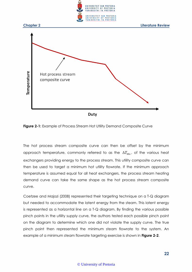
Figure 2-1: Example of Process Stream Hot Utility Demand Composite Curve
The hot process stream composite curve can then be offset by the minimum
approach temperature, commonly referred to as the MinT , of the various heat
exchangers providing energy to the process stream. This utility composite curve can
then be used to target a minimum hot utility flowrate. If the minimum approach
temperature is assumed equal for all heat exchangers, the process stream heating
demand curve can take the same shape as the hot process stream composite
curve.
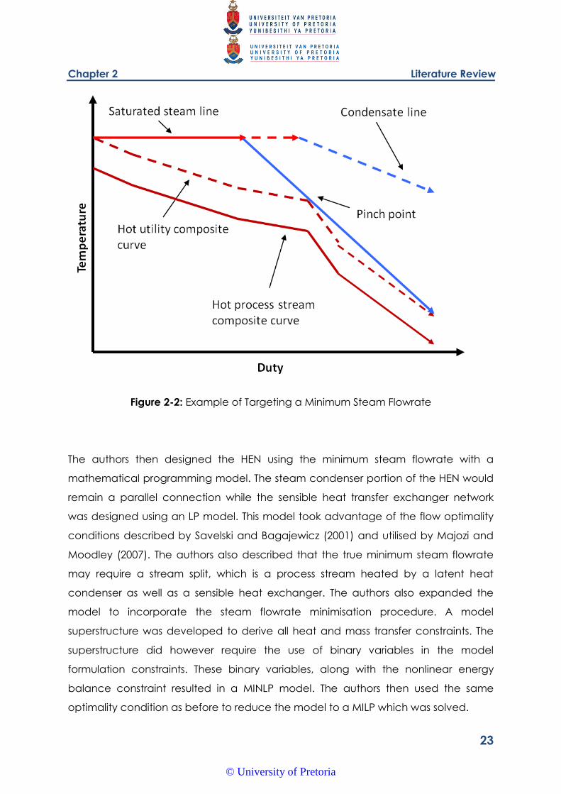
Coetzee and Majozi (2008) represented their targeting technique on a T-Q diagram
but needed to accommodate the latent energy from the steam. This latent energy
is represented as a horizontal line on a T-Q diagram. By finding the various possible
pinch points in the utility supply curve, the authors tested each possible pinch point
on the diagram to determine which one did not violate the supply curve. The true
pinch point then represented the minimum steam flowrate to the system. An
example of a minimum steam flowrate targeting exercise is shown in Figure 2-2.
© University of Pretoria
Chapter 2 Literature Review
23
Figure 2-2: Example of Targeting a Minimum Steam Flowrate
The authors then designed the HEN using the minimum steam flowrate with a
mathematical programming model. The steam condenser portion of the HEN would
remain a parallel connection while the sensible heat transfer exchanger network
was designed using an LP model. This model took advantage of the flow optimality
conditions described by Savelski and Bagajewicz (2001) and utilised by Majozi and
Moodley (2007). The authors also described that the true minimum steam flowrate
may require a stream split, which is a process stream heated by a latent heat
condenser as well as a sensible heat exchanger. The authors also expanded the
model to incorporate the steam flowrate minimisation procedure. A model
superstructure was developed to derive all heat and mass transfer constraints. The
superstructure did however require the use of binary variables in the model
formulation constraints. These binary variables, along with the nonlinear energy
balance constraint resulted in a MINLP model. The authors then used the same
optimality condition as before to reduce the model to a MILP which was solved.
© University of Pretoria
Chapter 2 Literature Review
24
Coetzee and Majozi (2008) extended the very effective utility optimisation
techniques developed for cooling systems to steam systems. They successfully
accounted for the latent energy of steam and reduced the steam flowrate using
both graphical and mathematical programming techniques. The authors however
only focused on the HEN itself, without investigating the effects on the steam boiler
or even system pressure drop.
2.3.1. Boiler Efficiency
Price and Majozi (2010a) followed on the work of Coetzee and Majozi (2008) and
included a provision for a steam boiler in the steam flowrate minimisation model. The
authors investigated the effects of a reduced steam flowrate and lower return
temperature on the operation of the steam boiler. The authors studied the effects
using the BHM derived by Shang and Kokossis (2004). The authors found that
reducing the steam flowrate and the subsequent reduction of the condensate
return temperature negatively affected the efficiency of the steam boiler. The
authors then attempted to reduce the steam flowrate to the HEN while maintaining
the boiler efficiency by more effectively pre-heating the boiler feed water stream.
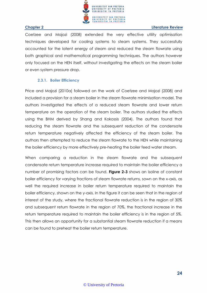
When comparing a reduction in the steam flowrate and the subsequent
condensate return temperature increase required to maintain the boiler efficiency a
number of promising factors can be found. Figure 2-3 shows an isoline of constant
boiler efficiency for varying fractions of steam flowrate returns, sown on the x-axis, as
well the required increase in boiler return temperature required to maintain the
boiler efficiency, shown on the y-axis. In the figure it can be seen that in the region of
interest of the study, where the fractional flowrate reduction is in the region of 30%
and subsequent return flowrate in the region of 70%, the fractional increase in the
return temperature required to maintain the boiler efficiency is in the region of 5%.
This then allows an opportunity for a substantial steam flowrate reduction if a means
can be found to preheat the boiler return temperature.
© University of Pretoria
Chapter 2 Literature Review
25
Figure 2-3: Sensitivity of Boiler Efficiency to Return Temperature and Flowrate
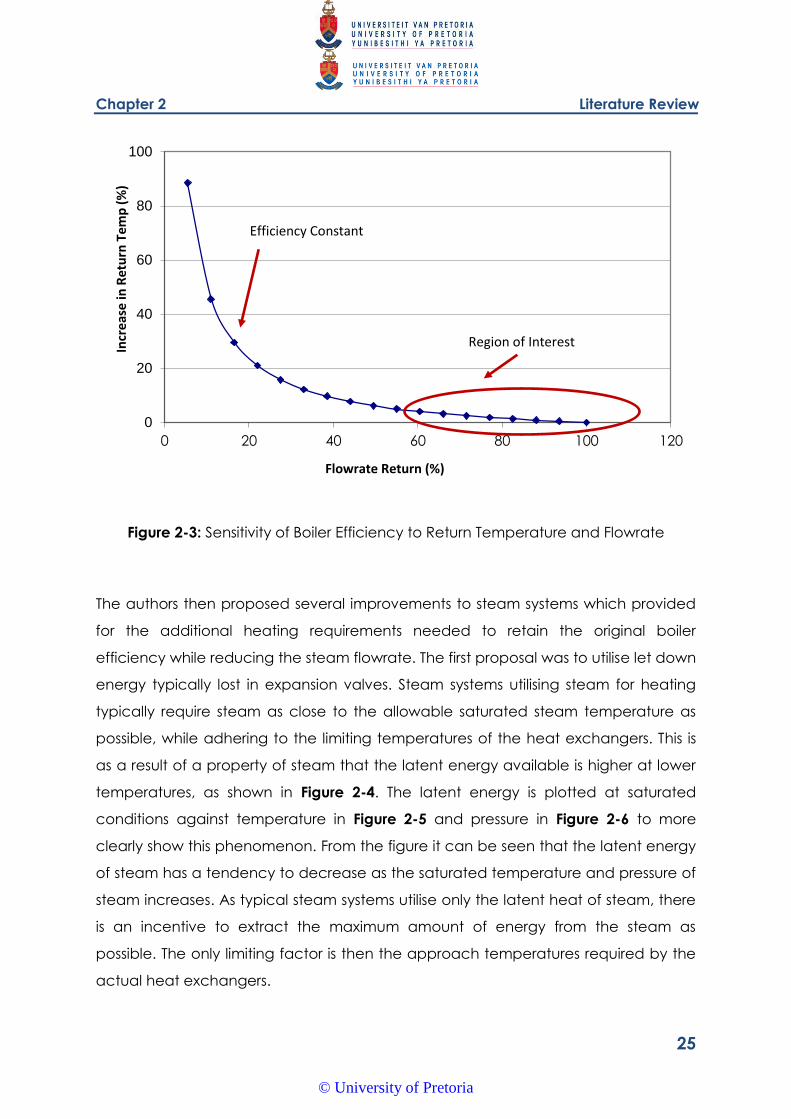
The authors then proposed several improvements to steam systems which provided
for the additional heating requirements needed to retain the original boiler
efficiency while reducing the steam flowrate. The first proposal was to utilise let down
energy typically lost in expansion valves. Steam systems utilising steam for heating
typically require steam as close to the allowable saturated steam temperature as
possible, while adhering to the limiting temperatures of the heat exchangers. This is
as a result of a property of steam that the latent energy available is higher at lower
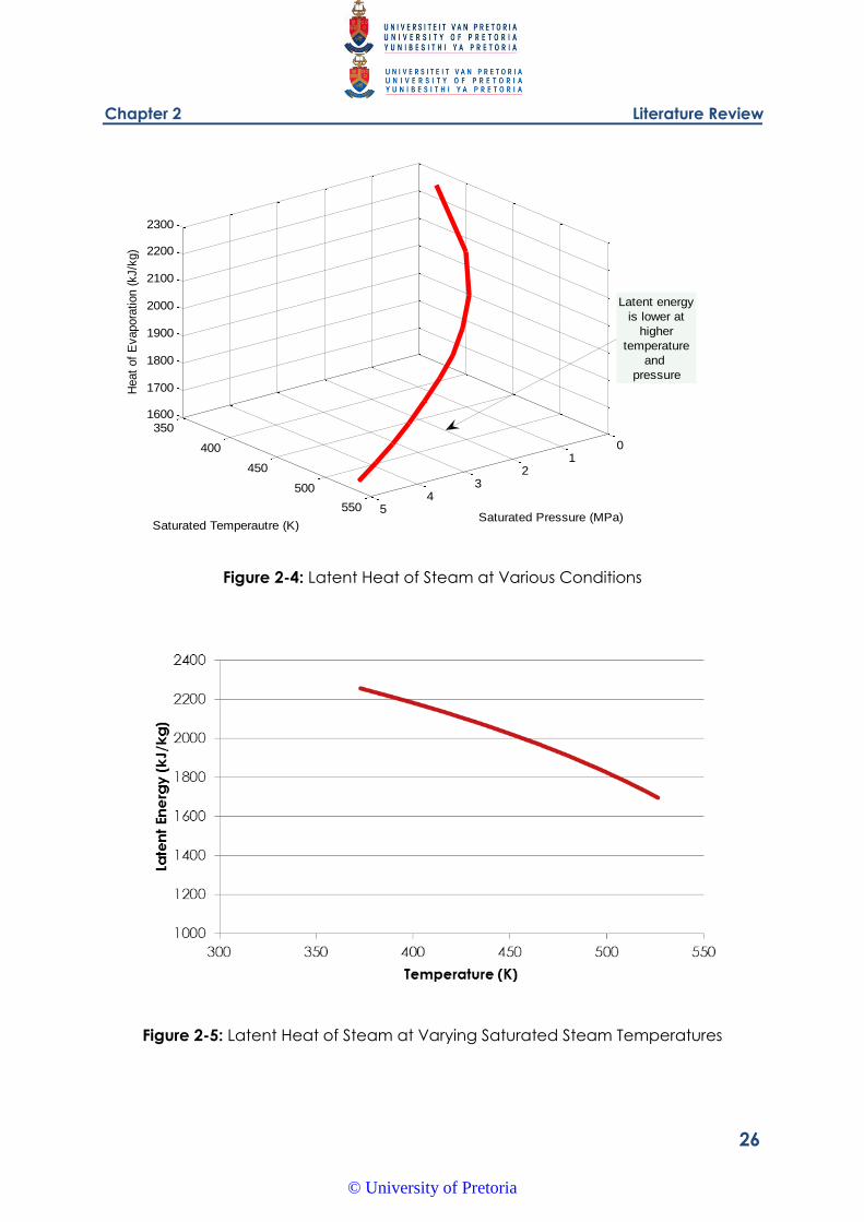
temperatures, as shown in Figure 2-4. The latent energy is plotted at saturated
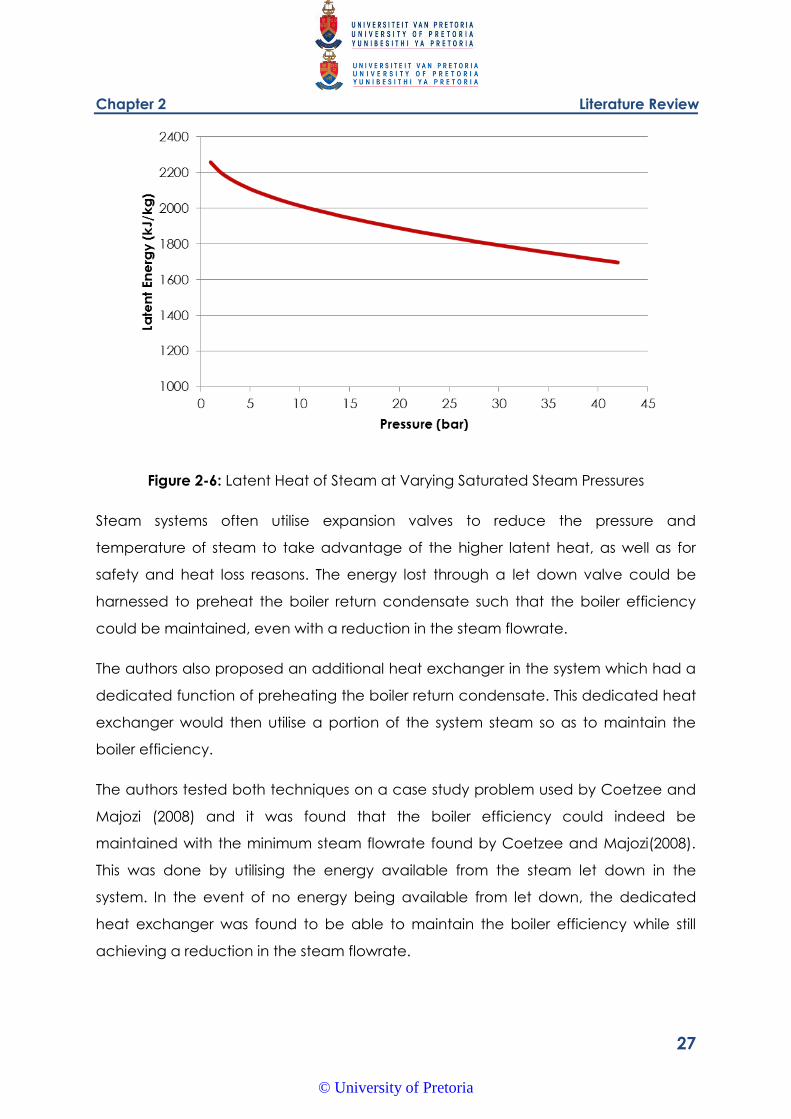
conditions against temperature in Figure 2-5 and pressure in Figure 2-6 to more
clearly show this phenomenon. From the figure it can be seen that the latent energy
of steam has a tendency to decrease as the saturated temperature and pressure of
steam increases. As typical steam systems utilise only the latent heat of steam, there
is an incentive to extract the maximum amount of energy from the steam as
possible. The only limiting factor is then the approach temperatures required by the
actual heat exchangers.
0
20
40
60
80
100
0 20 40 60 80 100 120
Incr
eas
e in
Ret
urn
Tem
p (
%)
Flowrate Return (%)
Efficiency Constant
Region of Interest
© University of Pretoria
Chapter 2 Literature Review
26
Figure 2-4: Latent Heat of Steam at Various Conditions
Figure 2-5: Latent Heat of Steam at Varying Saturated Steam Temperatures
01
23
45
350
400
450
500
550
1600
1700
1800
1900
2000
2100
2200
2300
Saturated Pressure (MPa)Saturated Temperautre (K)
Heat
of
Evapora
tion (
kJ/k
g)
Latent energy
is lower at
higher
temperature
and
pressure
© University of Pretoria
Chapter 2 Literature Review
27
Figure 2-6: Latent Heat of Steam at Varying Saturated Steam Pressures
Steam systems often utilise expansion valves to reduce the pressure and
temperature of steam to take advantage of the higher latent heat, as well as for
safety and heat loss reasons. The energy lost through a let down valve could be
harnessed to preheat the boiler return condensate such that the boiler efficiency
could be maintained, even with a reduction in the steam flowrate.
The authors also proposed an additional heat exchanger in the system which had a
dedicated function of preheating the boiler return condensate. This dedicated heat
exchanger would then utilise a portion of the system steam so as to maintain the
boiler efficiency.
The authors tested both techniques on a case study problem used by Coetzee and
Majozi (2008) and it was found that the boiler efficiency could indeed be
maintained with the minimum steam flowrate found by Coetzee and Majozi(2008).
This was done by utilising the energy available from the steam let down in the
system. In the event of no energy being available from let down, the dedicated
heat exchanger was found to be able to maintain the boiler efficiency while still
achieving a reduction in the steam flowrate.
© University of Pretoria

Chapter 2 Literature Review
28
Due to the presence of bilinear terms in the formulation, the models were solved as
MINLPs. The solution technique however utilised both the flow optimality conditions
of Savelski and Bagajewicz (2001) as well as the relaxation and linearisation
technique of Quesada and Grossmann (1995). These techniques allowed a linear
model to be solved and used as a starting point for the exact model.
The authors successfully incorporated more aspects of the steam system into an
optimisation framework. This holistic approach showed a pitfall in direct steam
flowrate reduction in the reduced efficiency of the steam boiler. The authors then
proposed a solution to maintain the boiler efficiency while still achieving the
minimum or at least a reduced steam flowrate. The authors did not however
consider other key aspects of HEN design, especially those related to rearranging
the HEN, such as network pressure drop. The work also focussed on a single system
steam level which does not encompass a large number of processes which utilise
multiple steam levels.
Price and Majozi (2010b) expanded on the author’s preceding work by
incorporating multiple pressure levels into the optimisation framework. These steam
levels are common in process plants and can originate from turbine exhaust. The
authors employed the same reuse and recycle flowrate minimisation approach as
well as the same techniques to maintain the boiler efficiency. The authors found that
by maximizing the use of the steam leaving the turbines, which was assumed to be
fixed, as well as the use of steam condensate for heating, the primary steam
flowrate to the HEN could be reduced while the boiler efficiency could also be
maintained.
A key factor in minimising steam flowrate in heating utility systems is the utilisation of
hot condensate to heat process streams that do not require high heating
temperatures. The rearrangement of the HEN as well as series nature of the retrofit
HEN are likely to lead to additional pressure drop in the steam utility network.
2.3.2. HEN Pressure Drop
Price and Majozi (2010c) then investigated the pressure drop effects of rearranging
the HEN from a parallel to a series based system. The authors followed a similar
approach to that of Kim and Smith (2003) whereby the HEN minimum flowrate was
© University of Pretoria
Chapter 2 Literature Review
29
first solved for and then used as a parameter in the pressure drop minimisation
problem. The steam flowrate minimisation model solved by Coetzee and Majozi
(2008) resulted in one of many HEN layouts which would lead to the minimum steam
flowrate. This meant that the network structure could then be further optimised for
an additional design variable such as pressure drop.
The authors constructed a node superstructure in a similar fashion to that of Kim and
Smith (2003). Additional nodes were included to account for the steam condensers.
The authors then formulated the pressure drop problem to minimise the maximum
pressure drop of the system using the critical path algorithm of Gass (1985).
Due to the nature of both the pressure drop as well as the heat and mass balance
superstructures binary variables were used to represent the existence of connections
and heat exchangers in the system. The energy balance constraints were linearised
using the optimality flow conditions of Savelski and Bagajewicz (2001). The pressure
drop correlations utilised by Kim and Smith (2003) were adapted for steam systems
and a condenser pressure drop correlation was added utilising approximations from
Frank (1978) and Kern (1950). The resulting binary variables and nonlinear constraints
meant the model was formulated as an MINLP.
The authors were successful in solving the model as an MINLP, however no indication
of the optimality of the result could be concluded. The solution procedure was
based on significant experience from Price and Majozi (2010c) where the authors
attempted to solve the heating system pressure drop minimisation problem in a
number of ways.
The authors attempted to solve the model by linearising the nonlinear pressure drop
correlations using piecewise linear approximations, which resulted in an MILP model.
Furthermore the authors attempted to solve the problem using the MILP problem as
the starting point for the exact model. The authors then also solved the model as an
MINLP directly. A comparison of the results showed the solution to the MINLP to be
more consistent among the various other design variables and to have a better
minimum pressure drop.
Price and Majozi (2010c) also encountered difficulties in solving the MINLP model
due to singularities in the nonlinear terms. The authors overcame these difficulties by
© University of Pretoria
Chapter 2 Literature Review
30
slightly relaxing the minimum steam flowrate and were able to solve the MINLP
model.
The authors Price and Majozi (2010c) were successful in formulating a pressure drop
minimisation model for steam systems which included the consideration of the steam
condensing units. The authors were able to find the minimum network pressure drop
while achieving a slightly higher steam flowrate than was shown by Coetzee and
Majozi (2008). The authors did not however adequately overcome the singularities
found in the solution of the MINLP and instead slightly relaxed the minimum steam
flowrate. The authors also did not fully explore the bounds of the HEN solution space
as the optimal flow conditions of Savelski and Bagajewicz (2001) fixed the heat
exchanger outlet temperatures to their minimum.
The series of papers by Price and Majozi (2010a, 2010b and 2010c) investigated the
holistic optimisation of heating systems and addressed a number of concerns with
steam flowrate reduction. Of these focus areas the optimisation of steam system
pressure drop was the least developed.
2.4. Conditions of Network Optimality
The conditions of optimality described in Savelski and Bagajewicz (2000a) play an
important role in network design with the intention of minimising the total water
intake. This work will be examined in slightly more detail and the scope of the
conditions, as well as degenerate solutions will be discussed. The application to HEN
design will also be mentioned.
The authors presented four theorems which were proven to hold when the solution
to a WAP was found to be optimal. The first was a condition of concentration
monotonicity, which stated that the concentration of a contaminant leaving a unit
cannot be lower than the combined concentration of all streams leading to that
unit. This essentially implied a net increase in concentration. The second required
that a unit that received only fresh water had an outlet concentration equal to its
maximum. This implied that the minimum fresh water is sent to these units. The third
required that units which received wastewater from certain units and then in turn
© University of Pretoria
Chapter 2 Literature Review
31
provided water to other units must have a maximum outlet concentration. Finally,
units that are fed by wastewater and return their wastewater to treatment should
have maximum outlet concentrations.
These theorems were then used to create a solution algorithm for designing a
network. Savelski and Bagajewicz (2001) then produced linear models to solve the
WAP problem which utilised the conditions of optimality. The key difference to their
approach as compared to previous attempts to use mathematical programming to
solve the problems was the condition stating that at least one optimal solution
existed where the outlet concentrations of all units were at their maximum. This
allowed the outlet concentration of the units to be fixed in the formulation,
eliminating bilinear terms which caused difficulties in the solution of previous models.
The authors first used the linearised models, formulated as LP or MILP problems
depending on the objective function, to solve for the minimum flowrate. The authors
then utilised the existence of multiple networks which exhibited the minimum
flowrate to further optimise the network. If the conditions of optimality were also
applied, the minimum flowrate could be added to the model as a constraint and
the model, now with a new objective function, could still be solved as an LP or MILP.
Aspects such as the minimum number of interconnections or minimum fixed cost
were some examples of objectives searched for with success. The authors also built
into their model the option to consider regeneration and what positive effects this
can have on the system.
One area briefly explored by the authors was degenerate solutions. The authors
stated that solutions can exist where the minimum freshwater intake is realised,
however the maximum outlet concentrations of units are not met. These solutions
are termed degenerate and the authors utilised these to further reduce the number
of connections in the system. The method used was fairly ad hoc and could
potentially be time consuming. It involved systematically increasing and decreasing
the freshwater utilised by certain key units and observing the resulting effects. The
authors stated that this could be done once the LP model is solved and the
minimum flowrate found as an additional means to further optimise an additional
variable. A disadvantage mentioned is an increased internal water flowrate. The
authors made mention of the fact that the degenerate solutions are infinite in
© University of Pretoria
Chapter 2 Literature Review
32
number and as such enumeration was futile. They further stated that no
mathematical model could make their proposed solution procedure more efficient.
The authors did allude to the fact that the conditions of optimality and their resulting
benefits would only hold if the relevant assumptions were true. As such, the authors
stated that the relationship between the outlet concentration and the wastewater
unit load should be investigated. The work presented was however an excellent
starting point for all investigations into the reduction of fresh water in wastewater
systems. The conditions of optimality also have implications in other network
optimisation fields such as HEN design. As such it was successfully utilised by Coetzee
and Majozi (2008) to reduce the steam mass flowrate to a HEN.
The authors did elaborate on the use of degenerate solutions, as well as the benefits
and shortcomings of such investigations. They presented an iterative approach to
investigating degenerate solutions however these solutions were not directly
incorporated into the optimisation framework and were rather considered once the
freshwater intake had been minimised. There is the possibility that degenerate
solutions can be utilised to further optimise utility networks, however the existence of
bilinear terms in the mathematical formulation of such problems is likely to be an
obstacle.
2.5. Some Mathematical Techniques for Nonlinear, Nonconvex Constraints
Bilinear terms are frequently found in chemical engineering applications where mass
flowrates are combined with a further variable to create the transfer of a medium
such as contaminant mass as well as utilities such as heat or materials such as
hydrogen. These bilinear terms are both nonlinear and nonconvex, making their
solution using NLP solvers difficult. This, combined with the superstructure type
arrangement prevalent in mathematical programming type network optimisation
frequently requires the use of binary variables to denote the existence or non-
existence of certain nodes and therefore problems are often formulated as MINLPs.
This section explores two techniques which have been formulated to simplify the use
of bilinear terms in literature as well as several notes on MINLP solvers.
© University of Pretoria
Chapter 2 Literature Review
33
2.5.1. Relaxation and Linearisation
Sherali and Alameddine (1992) approached the problem of bilinear terms by utilising
a relaxation and linearisation technique to simplify the nonconvex bilinear term into
a single variable. This variable was the product of the various bounds of the variables
constituting the original bilinear term. This approach was based on the convex and
concave envelopes used by McCormick (1976) to create over and under estimators
for bilinear terms in an attempt to simplify them. The approach by Sherali and
Alameddine (1992) was not a direct linearisation technique and as such this
programming approach does not always result in a feasible solution. The approach
did however propose an effective and simple linearisation for bilinear terms.
Quesada and Grossmann (1995) expanded on the work of Sherali and Alameddine
(1992) in their work with process networks. The authors attempted to optimise
network systems with multi-component flows where bilinear terms arose from mass
balance constraints. The networks in question consisted of a series of mixers, splitters
as well as linear process networks. The authors used the convex and concave
envelopes created by the variable bounds to replace the bilinear terms with a single
variable encapsulating the limits of the variable within its bounds. This linearised
solution was then solved and formed a lower bound on the optimisation problem.
This lower bound was then used as a starting point for the exact, nonlinear model.
Any feasible solution to the nonlinear model then formed an upper bound of the
current solution. The relaxed solution was then embedded within a branch and
bound procedure to obtain a solution.
The authors presented an algorithm which first defined effective bounds for the
variables making up the bilinear terms, then solved the relaxed model to form a
lower bound of the solution within the problem bounds and finally solved the exact
model within the same bounds. Due to the lower bound solution of the relaxed
problem, this algorithm was guaranteed to result in a globally optimal solution, within
a set tolerance, as stated by Sherali and Alameddine (1992).
Although the authors identified a limitation in the direct lack of application of the
algorithm to binary variable systems, the relaxation and linearisation formulation can
be extended to various sub-regions of the total solution space, allowing for the
© University of Pretoria
Chapter 2 Literature Review
34
application to systems which do contain binary variables. This work provided a
systematic means to optimise process networks, even with multi-component flows.
The authors utilised a relaxation and linearisation technique to reformulate bilinear
terms which held a large scope of application in many facets of network
optimisation. The algorithm presented by the authors was, in this form, limited to
processes with linear process units. The ability of the algorithm to find a tight lower
bound and effective starting point for the exact problem made this algorithm
applicable to many network type optimisation problems. This technique was used
successfully used by Majozi and Moodley (2007), Gololo and Majozi (2011) and
Gololo and Majozi (2013) to overcome bilinear terms in cooling network optimisation.
2.5.2. Transformation and Convexification
Bilinear terms are problematic to solve due to the nonconvex nature of the
constraints that contain them. Conventional NLP solvers typically utilise gradient
based methods to find an optimal solution, however nonconvex functions can lead
to local optimum results. Westerlund et.al. (1994) tried to formulate a pump
configuration as an MINLP problem. The authors utilised a variable number of pumps
in either a series or parallel configuration. The objective function for the formulation
caused complexity as it was nonlinear and nonconvex. The other constraints in the
problem were both equality and inequality constraints that were linear and
nonlinear. The authors propose an extended cutting plane (ECP) technique
combined with a general linear branch and bound technique to solve the resulting
MINLP. This work highlighted the complexity of proposing optimisation problems as
MINLP problems. The authors did however begin to consider techniques to simplify
the formulation and compare their proposed ECP technique to that of DICOPT + +
of Viswanathan and Grossmann (1990).
Westerlund and Petterssen (1995) furthered the development of the ECP method to
solve convex MINLP problems. The authors developed their own technique based on
NLP optimisation integer cuts first proposed by Kelley (1960). The binary variable
elements of the problem were handled using branch and bound techniques (Land
and Doig, 1960) or other mixed integer or mixed binary variable type solution
techniques by authors such as Van Roy and Wolsey (1987) or Crowder et al. (1983).
This method would be further developed by the authors, however a key limitation
© University of Pretoria
Chapter 2 Literature Review
35
was the restriction of the technique to solve problems with only convex nonlinear
constraints. Westerlund et al. (1998) presented a nonconvex MINLP problem solution
methods based on the ECP method. This method showed global optimum
convergence for pseudo convex problems, i.e. problems that contain nonconvex
terms, however in the operating region of the problem the terms are in fact found to
be convex. The method proposed by the authors sought to solve MINLP problems
with an iterative approach utilising the solution of MILP subproblems. This was quite
different from the conventional outer approximation solvers which employed MILP
master problems along with NLP subproblems.
Harjunkoski et al. (1997) explored the convexification of bilinear integer functions in
optimisation problems. The authors explored various mathematical transformations
to aid the optimisation of trim loss problems in the paper industry. The authors
recognised the existence of nonlinear, nonconvex terms in the mathematical
representation of the trim loss problem. The authors attempted to linearise or
transform bilinear terms containing discrete variables appearing in the formulation
into convex terms. The authors proposed four different linearisation approaches
which allowed the problem to be solved as a MILP or LP problem, however
consequently the number of variables and equations in the formulation increase
dramatically. The authors also proposed a convexification technique based on
transformations to exponential or square root functions, both of which are convex.
The problem was then solved using convex MINLP solvers such as the ECP. The
authors took an interesting approach to bilinear terms, opting to transform the terms
as oppose to replacing them.
Harjunkoski, Westerlund and Pörn (1999) formalised the transformation and
convexification of the bilinear terms in the trim loss problem and extended their
research into limiting the combinatorial space and reducing the size of the problem.
The authors also focussed on the benefits of carefully selecting an objective function
which not only minimised trimmed paper waste but also energy along with other
environmentally impacting variables. The authors discovered the benefit of keeping
several variables as part of the objective function. The authors also recognised
certain limitations to the heuristic approach of reducing the combinatorial solution
space and conceded that this area of work required specific attention. The authors
© University of Pretoria
Chapter 2 Literature Review
36
showed effective means of transforming bilinear terms into convex terms and
building these techniques into a solution procedure. Many MINLP solvers were
effective at solving convex problems and as such an effective convexification
technique could reduce difficult problems with bilinear terms to solvable problems,
perhaps even yielding globally optimum solutions.
Harjunkoski, Pörn and Westerlund (1999) continued to investigate the convexification
techniques for bilinear problems. The authors extend the application to several
example problems. They focused on the application of convex transformations over
linearisations and concluded that in certain cases convex transformations could
lead to the addition of fewer variables and constraints. Further, the authors explored
which of the transformations investigated led to tighter bounds, fewer variables and
better solution processes.
Following successful work with convex transformations, Pörn et al. (1999) discussed
general convexification techniques of bilinear terms consisting of discrete and
integer variables and in some cases continuous variables. They broached the
subject of posynomials, or products of variables to various powers, and stated the
prevalence of these variables in chemical engineering type optimisation problems.
They showed how discrete variables could be represented as integer variables, for
which more rigorous optimisation techniques exist such as the Glover transform
(Glover, 1975). The authors also showed that certain continuous functions were
convex, specifically exponential functions if the function was positive and
posynomial functions if the product of the powers was less than 1 and the term was
negative. Using appropriate inverse transformations, the authors could transform
nonconvex terms into convex terms and applied these to certain test problems. The
authors began to refer to these transforms as exponential transforms for positive
terms and potential transforms for negative terms. This work solidified the previous
advancements in this field by the authors and showed how problems could be
mathematically simplified. These simplifications could allow conventional solvers to
overcome numerical difficulties and possibly provide better solutions which are
globally optimal.
Pörn and Westerlund (2000) continued to develop the extended cutting plane
MINLP optimisation algorithm. The authors showed and proved the algorithm to
© University of Pretoria
Chapter 2 Literature Review
37
optimise pseudo-convex functions and this was demonstrated through further
example problems. The ECP MINLP solver was compared to other branch and
bound type MINLP solvers such as DICOPT (Viswanathan and Grossmann, 1990) by
Björk and Westerlund (2002) in their adaptation of the Synheat model of Yee and
Grossmann (1990). The authors utilised previously derived convexification techniques
to allow non-isothermal mixing of streams and as such allowed the already
comprehensive superstructure of Yee and Grossmann (1990) to allow for a larger
solution space and possibly a more optimal solution. The Synheat model of Yee and
Grossmann (1990) used this comprehensive HEN superstructure to attempt to
optimise cost by considering utilities, number of heat exchangers and heat
exchange area. This work showed the application of the convexification techniques
with already developed models. The uses of other optimisation algorithms such as
DICOPT were shown to be compatible and effective with convexification
techniques.
Björk et al. (2003) extended their research onto more comprehensive
convexifications. The authors attempted to create convex transformations of
signomial terms. Signomial terms are similar to polynomial terms, only with exponents
taking values of any real number. The authors showed how the choice of
transformation functions was essential in creating effective subproblems from the
transformed terms. The authors extended the exponential and potential
transformation techniques as well as showed how the concept of power convex
functions can be utilised to test the quality of the convexifications. The authors made
an important step in the work on convexification techniques by including signomial
terms which constituted exceptionally complex terms, as well as bilinear terms.
Pörn et al. (2008) then presented a global optimisation strategy for optimisation
problems with signomial parts. The authors presented a unified methodology to
transform signomial parts of constraints into convex terms on a term by term basis,
allowing already convex parts of the formulation to be unaffected. The
transformations were intended to create a convex lower bound of the problem
which could be solved by conventional methods. The transformations employed
were the exponential transform (ET) or the inverse transform (IT) for positively signed
terms as well as the potential transform (PT) for negatively signed terms. The
© University of Pretoria
Chapter 2 Literature Review
38
transformations did create nonconvex constraints which were discretised using a
piecewise linear approximation. The authors tested the transformations on a number
of test problems with promising results. The accuracy of the ET and IT were also
compared in this work and the ET was found to produce tighter lower bounds. The
authors stated that when problems were solved without a predefined starting point
the MINLP solution process could be expensive. This work did however provide a
formalised convexification tool to allow individual nonconvex terms of signomial
nature to be individually convexified. This had considerable potential to not only
make solution processes more efficient but also guarantee global optimality with
certain solvers such as αECP, DICOPT and BARON.
The transformation techniques themselves continued to be investigated. Lundell and
Westerlund (2009a) introduced a power transformation for positively signed
signomial terms and this was compared to the exponential transform. In more
detailed comparisons by Lundell and Westerlund (2009b) it was found that the
power transform only gave tighter lower bounds than the exponential transforms for
signomial terms of more than one variable in certain areas of the domain. Lundell
and Westerlund (2009c) then proposed a technique to find the optimal
transformations in nonconvex optimisation problems with signomial terms. The
authors developed an MILP method to optimally transform signomial terms as a pre-
processing step.
Lundell et al.(2013) then included the so called αBB-underestimator technique to
cater for the convexification of non-signomial functions which were twice
differentiable. Regular signomial terms are convexified using techniques already
described. The authors used the convexified formulation to create an
underestimation of the problem. This piecewise convex reformulation allowed the
entire problem to be solved using conventional MINLP solvers. This work further
solidified the advances of convexification strategies set out by Westerlund and his
co-workers.
The convexification of nonconvex terms is an important area of research as
nonconvex optimisation is abundant in the realistic modelling of systems. The
complexities caused by nonconvex terms therefore hamper the true optimisation of
such systems, however convexification strategies allow these problems to be solved
© University of Pretoria
Chapter 2 Literature Review
39
with a sense of the globally optimal nature of the solution. The use of piecewise
approximation in the ET, IT and PT transformations does require an iterative type
approach, however this will be discussed in later chapters of this work.
2.5.3. Notes on MINLP Solvers
A large number of commercial solvers have been created to solve MINLP problems.
Certain solvers are more suited to various applications due to internal heuristics.
Many successful solvers employ a two phase type optimisation approach utilising a
master problem in addition to subproblems. The MINLP problem is then split to create
NLP or relaxed LP problems combined with an MILP master problem. Such solvers
include the ECP type solvers of Westerlund and co-workers, DICOPT of Viswanathan
and Grossmann (1990) and BARON of Sahindis and Tawarmalani (2005).
The ECP methodologies evolved from early work with convex MINLP optimisation
based on work with integer cuts to solve nonlinear problems by Kelley (1960). The
methodology evolved to include the global optimisation of pseudo-convex
functions with the αECP solver (Pörn and Westerlund, 2000) which was updated and
introduced into the general algebraic modelling software (GAMS) optimisation
package with the title GAMS/AlphaECP. A comparison of this algorithm to other
MINLP solvers is found in Lastusilta et al. (2009) where it was found that the solver did
not solve as many NLP test problems as the best solver.
Baron is a relatively new addition to GAMS as compared to other solvers such as
DICOPT. Experience at the University of Pretoria is related to DICOPT with many
publications (Majozi and Moodley, 2008, Price and Majozi, 2010, Gololo and Majozi,
2013, and many others) having made use of the solver. DICOPT is an outer
approximation (OA) type solver, based on original work of Duran and Grossmann
(1986a), Duran and Grossmann (1986b) and Duran (1984). The solver essentially
deconstructs a MINLP problem into an MILP master problem by linearising the
nonlinear elements of the MINLP. An outer shell of the solution space is created using
these linearisations and the optimal solution is underestimated. The relaxed,
linearised master MILP problem is then solved. The resulting binary variables from this
solution are then fixed and the problem is solved as an NLP for that particular
arrangement of the binary variables. This process is repeated until a certain
© University of Pretoria
Chapter 2 Literature Review
40
tolerance is reached between the best underestimating master MILP solution and
that of an NLP solution. A large number of integer cuts are made to remove
infeasible solutions and to reduce the linearised solution space.
Before implementation in GAMS, DICOPT was further evolved by Kocis and
Grossmann (1987) where an equality-relaxation variation was added to the OA
formulation. Kocis and Grossmann (1988) then approached nonconvex MINLP
problems. The authors found that the MILP master problem could, on occasion,
remove the most optimal solution during linearisations when nonconvexities were
present in the nonlinear portion of the MINLP formulations. The authors proposed a
two phase approach to identify potentially nonconvex areas and where applicable
alter the MILP master problem. While the technique did not guarantee a globally
optimal solution, this strategy did focus attention on the key aspects of nonconvexity
in MINLP formulations. Kocis and Grossmann (1989a) discussed computational
experience with DICOPT for a large number of test problems. The authors noted a
key area of using DICOPT as the existence of nonconvexities in the model
formulations. Two areas of concern for the authors were the existence of local
optimal results in the NLP subproblems as well as sub optimal lower bounds in the
MILP master problem. The authors showed the flexibility of DICOPT but also pointed
out a key feature which should be addressed in model formulation. Kocis and
Grossmann (1989b) then presented a modelling and decomposition strategy for
process flowsheets so as to maximise the efficiency of DICOPT. The authors used
certain heuristics to replace nonconvex splitter representations with linear models in
choice areas. NLP subproblems were also limited to the particular flowsheet as
opposed to the entire superstructure. The size of the master problem was also
reduced using a lagrangian based decomposition scheme. The authors then
demonstrated these additional procedures using nonconvex test problems. The
authors recognised the aspects of nonconvexity as being potentially problematic for
DICOPT, however steps could be implemented to cater for these nonconvexities
and utilise the robust and effective solution procedure employed by DICOPT. A key
feature was recognising areas of potential difficulty and making modelling
alterations to cater for these situations. DICOPT forms part of the GAMS suite of
MINLP solvers (Viswanathan and Grossmann, 1990).
© University of Pretoria
Chapter 2 Literature Review
41
The intricacies of MINLP problems are the binary or discrete nature coupled with
nonlinearity. MINLP solvers need to efficiently tackle both. Key modelling changes
can greatly affect the solution of problems and diligent pre-processing should
always be conducted before utilising MINLP solvers. Nonconvexity has also been
pointed out as a key area, however advances in relaxation and linearisation
strategies such as that of Quesada and Grossmann (1995) or convexification
techniques such as that of Pörn et al. (2008) can be used to aid in the optimisation
of MINLP type problems.
2.6. Conclusion
This literature review has considered areas of HEN optimisation and the development
of techniques to optimise HEN in terms of utility flowrate as well as design aspects
such as network arrangement and the effects these have on aspects such as
pressure drop. It has been found that holistic approaches to systems yield the most
optimal results.
Flow networks are complicated systems to model as they often include bilinear terms
which are nonlinear and nonconvex. Conditions of optimality can allow optimal
networks to be designed from a flowrate minimisation perspective and bypass the
difficulty of bilinear terms. These conditions may however stifle attempts to further
optimise networks by limiting a key design variable and minimising the problem
solution space. Degenerate solutions have been shown to yield optimal utility
flowrates while also facilitating the optimisation of further design variables.
Degenerate solutions do however pose optimisation difficulties as bilinear terms must
be addressed. Techniques in literature have been developed to aid MINLP solvers in
the solution of problems with nonconvex terms.
In this work degenerate solutions will be exploited to further optimise HEN pressure
drop while utilising relaxation or convexification techniques to overcome bilinear
terms. The solution technique will then be applied to the entire steam system in an
attempt to maintain boiler efficiency with a reduced steam flowrate in a more
optimal way.
© University of Pretoria
Chapter 2 Literature Review
42
2.7. References
Ahmed, S. and Smith, R. (1989) Targets and design for minimum number of shells in
heat exchanger networks, Institute of Chemical Engineers ChERD, Vol 67, page 481.
Alva-Argáez, A, Kokossis, A. C. and Smith, R. (1998) Wastewater Minimisation of
Industrial Systems Using an Integrated Approach, Computers and Chemical
Engineering, 22, 741-744.
Asante, N.D.K. and Zhu, X.X. (1997) An Automated and interactive approach for
heat exchanger network retrofit, Chemical Engineering Research and Design, 75 (3),
349-360.
Bernier, M. A. (1994) Cooling tower performance: Theory and experiments, ASHRAE
Transactions Res, 100, pages 114-121.
Björk, K, Lindberg, P. O. and Westerlund, T. (2003) Some convexifications in global
optimization of problems containing signomial terms, Computers and Chemical
Engineering, 27, 669-679.
Bjork, K. and Westerlund, T. (2002) Global optimization of heat exchanger network
synthesis problems with and without the isothermal mixing assumption, Computers
and Chemical Engineering, 26, 1581-1593.
Coetzee, W. A. and Majozi, T. (2008) Steam System Network Design Using Process
Integration, Industrial Engineering Chemistry Research 2008, 47, 4405-4413.
Crowder, H, Johnson, E. L. and Padberg, M. (1983) Solving Large-Scale Zero-One
Linear Programming Problems, Operations Research 1983, 31, 803-834.
Doyle, S. J. and Smith, R. (1997) Targeting Water Reuse with Multiple Contaminants,
Process Safety and Environmental Protection 1997, 75, 181-189.
Duran, M, A. (1984) A Mixed-Integer Nonlinear Programming Approach for the
Systematic Synthesis of Engineering Systems, Pittsburgh: Carnegie-Mellon University.
© University of Pretoria
Chapter 2 Literature Review
43
Duran, M. A. and Grossmann, I. E. (1986a) A Mixed-Integer Nonlinear Programming
Algorithm for Process Systems Synthesis, American Institute of Chemical Engineering
Journal, 32, No. 4, 592-606.
Duran, M. A. and Grossmann, I. E. (1986b) An Outer-Approximation Algorithm for a
Class of Mixed Integer Nonlinear Programs, Mathematical Programming, 36, 3, 307-
339.
El-Halwagi, M. M. and Manousiouthakis, A. M. (1989) Synthesis of mass-exchange
networks, American Institute of Chemical Engineering Journal, 8, 1233-1244.
El-Halwagi, M. M. and Manousiouthakis, A. M. (1990) Automatic synthesis of mass-
exchange networks with single component targets, Chemical Engineering Science,
9, 2813-2831.
Frank, O. (1978) Simplified design procedure for tubular exchangers, Practical
aspects of heat transfer, Chem. Eng. Prog. Tech. Manual (Am. Inst. Chem. Eng).
Gass, S. I. (1985) Linear Programming, 5th Edition, Mcgraw-Hill, New York.
Glover, F. (1975) Improved linear integer programming formulation of nonlinear
problems, Management Science, Pages 455-460.
Gololo, K. V. and Majozi, T. (2011), On Synthesis and Optimization of Cooling Water
Systems with Multiple Cooling Towers, Industrial Engineering Chemistry Research
2011, 50 (7), 3775−3787.
Gololo, K. V. and Majozi, T. (2013) Complex Cooling Water Systems Optimization with
Pressure Drop Consideration, Industrial Engineering Chemistry Research, 52,
7056−7065.
Harjunkoski, I, Pörn, R, Westerlund, T. and Skrifvars, H. (1997) Different Strategies for
Solving Bilinear Integer Nonlinear Programming Problems with Convex
Transformations, Computers and Chemical Engineering, 21, 487-492.
Harjunkoski, I, Westerlund, T. and Pörn, R. (1999) Numerical and environmental
considerations on a complex industrial mixed integer nonlinear programming
(MINLP), Computers and Chemical Engineering, 23 , 1545–1561.
© University of Pretoria
Chapter 2 Literature Review
44
Hohmann, E. C. (1971) Optimum networks for heat exchange, Ph.D. Thesis, University
of Southern California.
Huang, C. H, Chang, C. T, Ling, H. C. and Chang, C. C. (1999) A Mathematical
Programming Model for Water Usage and Treatment Network Design. Industrial
Engineering Chemistry Research 1999, 38, 2666.
Huang, F. and Elshout, R. V. (1976) Optimizing the heat recovery of crude units,
Chemical Engineering Programming, 72, pages 68-74.
Jegede, F. O. (1990) Power, capital and energy cost trade-offs in heat exchanger
networks, Ph.D. Thesis, UMIST, Manchester.
Jegede, F. O. and Polley, G. T. (1992) Optimum heat exchanger design, Transactions
of Institute of Chemical Engineers, Vol 70 (part A), pages 133-141.
Kelley, J. E. (1960) The Cutting Plane Method for Solving Convex Programs, Journal of
the SIAM 1960, 8, 703–712.
Kern, D. Q. (1950) Process heat transfer, Mcgraw Hill, New York.
Kim, J. K. and Smith, R. (2001) Cooling water system design, Chemical Engineering
Science, Vol 56, pages 3641-3658.
Kim, J. K. and Smith, R. (2003) Automated retrofit design of cooling-water systems,
Process Systems Engineering, Vol 49, No7, pages 1712-1730.
Kocis, G. R. and Grossmann, I. E. (1987) Relaxation Strategy for the Structural
Optimization of Process Flow Sheets, Industrial Engineering Chemistry Research, 26,
1869-1880.
Kocis, G. R. and Grossmann, I. E. (1988). Global Optimization of Nonconvex Mixed-
Integer Nonlinear Programming (MINLP) Problems in Process Synthesis. Industrial
Engineering Chemistry Research 1988, 27, 1407-1421.
Kocis, G. R. and Grossmann, I. E. (1989a) A Modelling and Decomposition Strategy
for MINLP Optimization of Process Flowsheets. Computers and Chemical Engineering
1989, 13 (7), 797-819.
© University of Pretoria
Chapter 2 Literature Review
45
Kocis, G. R. and Grossmann, I. E. (1989b) Computational Experience with DICOPT
Solving MINLP Problems in Process Systems Engineering. Computers and Chemical
Engineering 1989, 13 (3), 307-315.
Kuo, W. C. J. and Smith, R. (1998) Design for the interactions between water-use and
effluent treatment, Institution of Chemical Engineers Trans IChem, Vol 76, Part A,
pages 287-301.
Land, A. H. and Doig, A. (1960) An Automatic Method of Solving Discrete
Programming Problems, Ecometrica 1960, 28, 497-520.
Lastusilta, T, Bussieck, M. R. and Westerlund, T. (2009) An experimental study of the
GAMS/AlphaECP MINLP solver, Industrial Engineering Chemistry Research, 48, 15,
7337-7345.
Linnhoff, B. and Flower, J. R. (1978) Synthesis of heat exchanger networks, Part I.
Systematic generation of energy optimal networks, A.I.Ch.E.J, Vol 24, page 633.
Linnhoff, B. and Hindmarsh, E. (1982) The Pinch method for heat exchanger network,
Chemical Engineering Science, Vol 38, No 5, pages 745-763.
Linnhoff, B. Mason, D. R. and Wardle, I. (1979) Understanding heat exchanger
networks, Computers and Chemical Engineering, Vol 3, pages 295-302.
Lundell, A. and Westerlund, T. (2009a) Implementation of a Convexification
Technique for Signomial Functions, European Symposium on Computer Aided
Process Engineering, Cracow, Elsevier. 579-582.
Lundell, A. and Westerlund, T. (2009b) On the Relationship between Power and
Exponential Transformations for Positive Signomial Functions, Chemical Engineering
Transactions, 17, 1287-1292.
Lundell, A. and Westerlund, T. (2009c) Optimization of Transformations for Convex
Relaxations of MINLP Problems Containing Signomial Functions, International
Symposium on Process Systems Engineering, Salvador, Bahia, Brazil, Elsevier, 231-236.
Lundell, A. Skjäl, A. and Westerlund, T. (2013) A reformulation framework for global
optimization, Journal of Global Optimization, 57, 115-141
© University of Pretoria

Chapter 2 Literature Review
46
Majozi, T. and Moodley, A. (2008) Simultaneous targeting and design for cooling
water systems with multiple cooling water supplies, Computers and Chemical
Engineering, Vol 32, pages 540-551.
Mavromatic, S. P. and Kokossis, A. C. (1998) Conceptual optimisation of utility
networks for operational variations. 1. Targets and level optimisation, Chemical
Engineering Science, Vol 53, page 1585.
McCormick, G. (1976) Computability of global solutions to factorable nonconvex
programs. Part I Convex underestimating problems.
Nie, X. and Zhu, X. X. (1999) Heat exchanger retrofit considering pressure drop and
heat transfer enhancement, A.I.Ch.E.J, Vol 45, page 1239.
Nie, X. and Zhu, X. X. (2002) Pressure drop considerations for heat exchanger
grassroots design, Computers and Chemical Engineering, Vol 26, pages 1661-1676.
Nie, X. R. (1998) Heat exchanger network retrofit considering pressure drop and heat
transfer enhancement, Ph.D. Thesis, UMIST, Manchester.
Olesen, S. G. and Polley, G. T. (1996) Dealing with Plant Geography and Piping
Constraints in Water Network Design, Process Safety and Environmental Protection
1996, 74, 273-276.
Papoulias, S. A. and Grossmann, I. E. (1983a) A structural optimization approach in
process synthesis – I Utility systems, Computers and Chemical Engineering, Vol 7, No
6, pages 695-706.
Papoulias, S. A. and Grossmann, I. E. (1983b) A structural optimization approach in
process synthesis – II Heat recovery networks, Computers and Chemical Engineering,
Vol 7, No 6, pages 707-721.
Papoulias, S. A. and Grossmann, I. E. (1983c) A structural optimization approach in
process synthesis – III Total processing systems, Computers and Chemical
Engineering, Vol 7, No 6, pages 723-734.
Pattison, J. R. and Sharma, V. (1980) Selection of boiler plant and overall system
efficiency, Studies in energy efficiency in buildings, British Gas.
© University of Pretoria
Chapter 2 Literature Review
47
Peters, M. S. and Timmerhaus, K. D. (1991) Plant design and economics for chemical
engineers, 4th Edition, Mcgraw-Hill, New York.
Pörn, R, Harjunkoski, I. and Westerlund, T. (1999) Convexification of different classes of
nonconvex MINLP problems, Computers and Chemical Engineering, 23 , 439-448.
Pörn, R. and Westerlund, T. (2000) A cutting plane method for minimizing pseudo-
convex functions in the mixed integer case, Computers and Chemical Engineering,
24, 2655–2665.
Pörn, R., Bjork, K., and Westerlund, T. (2008) Global solution of optimization problems
with signomial parts. Discrete Optimization 5 , 108-120.
Price, T. and Majozi, T. (2010a) On Synthesis and Optimization of Steam System
Networks. 1. Sustained Boiler Efficiency. Industrial Engineering Chemistry Research 49
, 9143–9153.
Price, T. and Majozi, T. (2010b) Synthesis and Optimization of Steam System Networks.
2. Multiple Steam Levels. Industrial Engineering Chemistry Research 49 , 9154–9164.
Price, T. and Majozi, T. (2010c) On Synthesis and Optimization of Steam System
Networks. 3. Pressure Drop Consideration. Industrial Engineering Chemistry Research
49 , 9165–9174.
Quesada, I. and Grossmann, I. E. (1995) Global optimisation of bilinear process
networks with multi component flows, Computers and Chemical Engineering 19, No
12, pages 1219-1242.
Sahinidis, N. and Tawamalani, M. (2005) BARON. In GAMS The Solver Manuals (pp. 9-
22). Washington: GAMS Development Corporation.
Savelski, M. J. and Bagajewicz, M. J. (2000a) Design of Water Utilization Systems in
Process Plants with a Single Contaminant, Waste Management 2000, 20, 659-664.
Savelski, M. J. and Bagajewicz, M. J. (2000b) On the optimality conditions of water
utilization systems in process plants with single contaminants, Chemical Engineering
Science 55, pages 5035-5048.
© University of Pretoria
Chapter 2 Literature Review
48
Savelski, M. J. and Bagajewicz, M. J. (2001), On the Use of Linear Models for the
Design of Water Utilization Systems in Process Plants with a Single Contaminant,
Institution of Chemical Engineers, Trans IChemE 2001 , 79, Part A, 600-610.
Savelski, M. J. and Bagajewicz, M. J. (2003) On the necessary conditions of optimality
of water utilization systems in process plants with multiple contaminants. Chemical
Engineering Science , 58, 5349-5362.
Shang, Z. and Kokossis, A. (2004) A transhipment model for the optimisation of steam
levels of total site utility system for multiperiod operation, Computers and Chemical
Engineering 28, pages 1673-1688.
Sherali, H. D. and Alameddine, A. (1992). A New Reformulation-Linearization
Technique for Bilinear Programming Problems. Journal of Global Optimization , 2,
379-410.
Sinnot, R. K. (2005) Chemical engineering design, Vol 6, Elsevier Butterworth
Heinemann, New York.
Skjäl, A, Lundell, A. and Westerlund, T. (2011) Global Optimization with c2 Constraints
by Convex Reformulations, Chemical Engineering Transactions, 24, 373-378.
Takama, N, Kuriyama, T, Shiroko, K. and Umeda, T. (1980) Optimal water allocation in
a petroleum refinery, Computers and Chemical Engineering, Vol 4, pages 251-258.
Umeda, T. Harada, T. and Shiroko, K. (1979) A thermodynamic approach to the
synthesis of heat integration systems in chemical processes, Computers and
Chemical Engineering, Vol 3, pages 273-282.
Van Roy, T. J. and Wolsey, L. A. (1987) Solving Mixed 0-1 Programs by Automatic
Reformulation, Operations Research 1987, 35, 45-57.
Viswanathan, J. and Grossmann, I. E. (1990) A Combined Penalty Function and
Outer-Approximation Method for MINLP Optimization, Computers and Chemical
Engineering, Vol 7, pages 769-782.
© University of Pretoria
Chapter 2 Literature Review
49
Viswanathan, J. and Grossmann, I. E. (1990) A Combined Penalty Function and
Outer-Approximation Method for MINLP Optimization, Computers and Chemical
Engineering, Vol 7, pages 769-782.
Wang, Y. P. and Smith, R. (1994) Wastewater minimisation, Chemical Engineering
Science, Vol 49, page 981.
Westerlund, T, Pettersson, F. and Grossmann, I. E. (1994) Optimization of Pump
Configurations as a MINLP Problem. Computers and Chemical Engineering 18 , 845-
858.
Westerlund, T. and Pettersson, F. (1995) An Extended Cutting Plane Method for
Solving Convex MINLP Problems, Computers and Chemical Engineering 1995, 19 ,
131-136.
Westerlund, T. Skrifvars, H. Harjunkoski, I. and Pörn, R. (1998) An extended cutting
plane method for a class of nonconvex MINLP problems, Computers and Chemical
Engineering, 22 , 357-365.
Yee, T. F. and Grossmann, I. E. (1990) Simultaneous optimization models for heat
integration - II. Heat exchanger network synthesis, Computer and Chemical
Engineering, 1, 1165.
Zhu, X. X, O’Neil, B. K, Roach, J. R. and Wood, R. M. (1995) A new method for heat
exchanger network synthesis using area targeting procedures, Computers and
Chemical Engineering, Vol 19, pages 197-222.
© University of Pretoria
Chapter 3 Motivation for Study
50
3. Motivation for Study
This chapter discusses the general background to the work presented in this thesis.
The topics include previous work, heat exchanger network pressure drop, boiler
efficiency, degenerate solutions of flow networks and the general principals of some
MINLP solvers.
3.1. Background
This section is intended to give a background and motivation for further investigation
of heat exchanger network pressure drop. Techniques developed in this work will
then also be applied to other aspects of steam system HEN optimisation such as
boiler efficiency.
3.1.1. Previous Work
Utility system optimisation has been explored by Majozi and co-workers for both
batch and continuous systems. The focus of this thesis is specifically continuous
steam system optimisation.
Coetzee and Majozi (2008) minimised the steam flowrate required for HENs by
utilising sensible heat from steam condensate to heat process streams along with the
latent heat from the steam. The subsequent effects on the steam boiler efficiency
were addressed by Price and Majozi (2010a) while the pressure drop effects of
adding series connections to utilise condensate to the HEN were investigated by
Price and Majozi (2010c).
Price and Majozi (2010c) formulated the pressure drop model using a novel
superstructure to develop flow and pressure drop constraints. The resulting
formulation was presented as an MINLP. The authors attempted to simplify the
formulation to create an MILP using various techniques. These included those
employed by Glover (1975) to cater for bilinear terms involving binary variables as
well as that of Quesada and Grossmann (1995). The resulting techniques were found
to be ineffective and the best solution to the pressure drop formulation came from
© University of Pretoria
Chapter 3 Motivation for Study
51
solving the problem as an MINLP. Slight flow relaxations were required in order for a
feasible solution to be found. The MINLP used to represent the HEN pressure drop
problem is complex due to binary variables present in the formulation as well as the
nonconvex nature of the bilinear terms making up formulation.
The authors identified the need to further explore the steam system HEN pressure
drop problem. The key aspect of solving the pressure minimisation problem is to do
so while still achieving the minimum steam flowrate for the system. In this way two or
more design variables, steam flowrate as well as an additional variable such as
network pressure drop, can be minimised in order to reduce the cost of grassroots
designs or debottleneck existing steam systems. Any techniques developed will then
also be applied to other aspects of HEN optimisation such as pressure drop.
This work is intended to build from the experience of and Price and Majozi (2010c).
The model formulation will be deconstructed in an attempt to solve the pressure
drop problem with the exact minimum steam flowrate as described by the method
of Coetzee and Majozi (2008). The assumptions and simplifications utilised by
preceding authors to this work such as Coetzee and Majozi (2008) will also be
examined in an attempt to find a better minimum pressure drop solution.
Certain formulations developed by Price and Majozi (2010a) used to maintain boiler
efficiency also exhibit bilinear terms in the MINLP formulation. Therefore any
techniques developed to aid the HEN pressure drop minimisation problem will also
be applied to those complex MINLP formulations intended to maintain boiler
efficiency.
3.1.2. Modelling Experience
Majozi and co-workers have large amounts of network optimisation experience.
Certain features of flow networks make optimisation of such systems difficult to solve,
the most prevalent of which are bilinear terms. Bilinear terms exhibit nonconvex,
nonlinear properties which cause difficulties for most MINLP solvers. An additional
complexity for some systems is the batch nature of the operations which have an
additional time component which adds an additional number of complicated
constraints when optimising batch systems.
© University of Pretoria
Chapter 3 Motivation for Study
52
A number of simplification and optimisation techniques are used by Majozi and his
co-workers. These include simplifying systems using the relaxation and linearisation
technique of Quesada and Grossmann (1995), formerly of Sherali and Alameddine
(1992). This technique allows bilinear terms to be linearised and models to be solved
as MILPs. This technique has been used by many researchers to optimise a number
of networks involved in heat exchange and wastewater minimisation. Glover
transforms allow bilinear terms formed from a single continuous and a single binary
term to be considered as a single variable in the formulation. Optimal mass
exchange unit outlet conditions as described by Savelski and Bagajewicz (2000)
have been proved to yield optimal flow conditions in mass exchange networks and
this was successfully used to optimise heat exchange networks by Coetzee and
Majozi (2008) as certain principles of mass and heat transfer are interchangeable.
While techniques are available in literature to handle a number of complex
constraints encountered by Majozi and co-workers, a number of alternative
techniques can be used to overcome these difficulties. Further understanding of
network flow models as well as alternative constraint formulation can also be used
to optimise these problems.
3.2. System of Interest
The steam system in the context of this investigation is shown in Figure 3-1. The boiler
unit produces superheated high pressure steam, shown as stream 1. This steam can
then proceed to a let down valve as stream 2 or can proceed to a high pressure
steam turbine as stream 3. Stream 1 is superheated high pressure steam, however
the heating utility for processes is typically saturated steam. This is due to the parallel
configuration typically seen in HENs. Each heat exchanger receives saturated
steam and latent energy is used to heat the appropriate process stream. A let down
valve provides a means to reduce the pressure of stream 2 such that it becomes
saturated steam as in stream 4.
© University of Pretoria
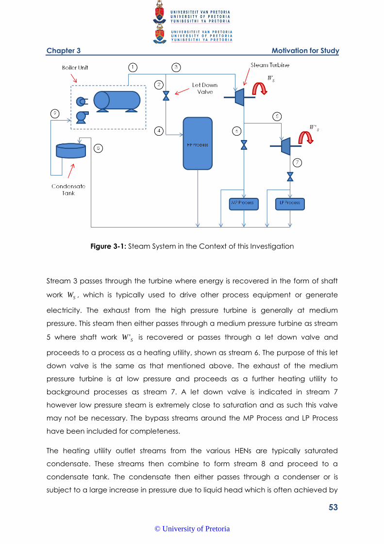
Chapter 3 Motivation for Study
53
Figure 3-1: Steam System in the Context of this Investigation
Stream 3 passes through the turbine where energy is recovered in the form of shaft
work SW , which is typically used to drive other process equipment or generate
electricity. The exhaust from the high pressure turbine is generally at medium
pressure. This steam then either passes through a medium pressure turbine as stream
5 where shaft work SW ' is recovered or passes through a let down valve and
proceeds to a process as a heating utility, shown as stream 6. The purpose of this let
down valve is the same as that mentioned above. The exhaust of the medium
pressure turbine is at low pressure and proceeds as a further heating utility to
background processes as stream 7. A let down valve is indicated in stream 7
however low pressure steam is extremely close to saturation and as such this valve
may not be necessary. The bypass streams around the MP Process and LP Process
have been included for completeness.
The heating utility outlet streams from the various HENs are typically saturated
condensate. These streams then combine to form stream 8 and proceed to a
condensate tank. The condensate then either passes through a condenser or is
subject to a large increase in pressure due to liquid head which is often achieved by
© University of Pretoria
Chapter 3 Motivation for Study
54
elevating the condensate tank. This is to ensure the condensate is sufficiently far
away from the saturation temperature so as to prevent the risk of cavitation during
pumping to the steam boiler. The risk of cavitation is mostly associated with
centrifugal pumps which are the most prevalent in boiler systems. Make up water is
also typically added in this region although this has been omitted for simplicity. The
stream proceeding to the boiler feed water pump is shown as stream 9. After being
pumped the return stream to the boiler passes through a pre heater or economiser
to heat the boiler feed. The economiser is often found as part of a commercial boiler
package.
The steam lost during let down is typically collected in flash drums which have been
excluded from Figure 3-1 for simplicity. Typically the supply temperature of steam to
a HEN is designed as close to the highest limiting utility supply temperature of the
HEN. This is due to the property of steam where latent energy per unit mass of steam
decreases as the temperature and pressure of the steam increases. Thus the steam
leaving the let down valve as stream 4 is at a lower pressure than stream 2. This is
referred to as the process pressure from here onwards.
HEN pressure drop will be explored within the individual HEN processes, whereas
boiler efficiency will include all elements of Figure 3-1.
3.3. HEN Pressure Drop
This section is intended to explore some of the complexities of pressure drop in a flow
network.
3.3.1. Background to HEN Pressure Drop
The steam flowrate to a heating utility heat exchange network can be considerably
reduced if energy is further harnessed from the saturated and sub cooled
© University of Pretoria
Chapter 3 Motivation for Study
55
condensate leaving condensers. This is achieved by recycling and reusing
condensate where possible. A technique to systematically achieve the minimum
steam flowrate is presented in Coetzee and Majozi (2008). One concern with the
recycle and reuse of condensate is the effect on the steam boiler. A means to
achieve the minimum steam flowrate while maintaining boiler efficiency was
presented by Price and Majozi (2010a). Price and Majozi (2010b) then reduced the
steam required for HENs where multiple steam levels are available and presented a
means of still maintaining the required boiler efficiency.
A further concern for recycle and reuse in HENs is the aspect of increased pressure
drop within the network. With recycling hot condensate, utility streams have to pass
through multiple heat exchangers in series which greatly increase the pressure drop
of the system. Kim and Smith (2003) identified the need to minimise pressure drop in
such networks from their work in cooling systems. From the work of Savelski and
Bagajewicz (2000), Coetzee and Majozi(2008) found that multiple networks could be
found for the same minimum flowrate due to the linear nature of the network design
model. Thus a further objective function could be applied to these optimum flow
networks. Additional objectives could include cost or pressure drop. Following a
similar approach to Kim and Smith (2003), pressure drop was minimised for a HEN in
steam systems by Price and Majozi (2010c).
In HENs pressure can be lost through pipes, condensate heat exchangers and
condensers. The mixing and splitting junctions that redirect flow can be considered
as part of the piping network. Pressure drop correlations are therefore needed in the
form of constraints so as to incorporate this into an optimisation framework.
Many correlations exist in literature, however those used by Kim and Smith (2003) are
the most appropriate as they are readily integrated with flowrate which is a variable
typically used in heat and mass exchange network optimisation problems. The
correlations are derived from the work of Nie (1998). These derivations will be
summarised for heat exchangers, condensers and pipework. The author represents
pressure drop through conventional shell and tube heat exchangers. Thus it will be
assumed that these heat exchangers are used in the investigation
© University of Pretoria
Chapter 3 Motivation for Study
56
Heat Exchanger and Condenser Pressure Drop
The tube side pressure drop for a heat exchanger is much more easily determined
than the shell side pressure drop as determined by Nie (1998). As such it will be
assumed that steam and condensate pass through the tube side of the heat
exchanger.
The pressure drop function presented by Kim and Smith (2003) is shown in Constraint
( 3-1 ).
2
2
8.1
1 ttttt VNVNP ( 3-1 )
In this constraint the tube side pressure drop is calculated with respect to the tube
side fluid velocity. Kim and Smith (2003) then convert this velocity constraint to one
with respect to volumetric flowrate, as seen in Constraint ( 3-1 ). According to Nie
(1998) the two terms account for the pressure drop as a result of the friction loss in
the tubes and the loss as a result of sudden contractions, expansions and flow
reversals. The two factors 1tN and 2tN are shown in Constraints ( 3-2 ) and ( 3-3 )
below.
8.48.2
8.28.08.0
8.21
115567.1
iot
tp
tddN
AnN
( 3-2 )
42
3
22
20
it
tp
tdN
nN
( 3-3 )
In Constraints ( 3-1 ), ( 3-2 ) and ( 3-3 ), tP is the tube side pressure drop, tV is the
tube side volumetric flowrate, is the fluid density, is the fluid viscosity, tpn is the
© University of Pretoria
Chapter 3 Motivation for Study
57
number of tube passes, A is the heat transfer area, tN is the number of tubes, od is
the outside tube diameter and id is the inside tube diameter.
Kim and Smith (2003) utilise certain industrial design guidelines to help approximate
realistic heat exchanger parameters such as heat exchange area, tube number
and tube diameter. Many of these terms in these constraints such as the heat
transfer area, the number of tubes and the tube dimensions are very much
interrelated in heat exchanger design. These guidelines, as well as those used for this
work, are discussed in Appendix A.
The pressure drop for condensers must also be catered for as they also appear in
HENs utilising steam as a heating medium. According to Sinnot (2005), the pressure
drop through condensers where total condensation occurs can be approximated
by calculating the pressure drop in the conventional fashion using the inlet vapour
conditions and multiplying this by a factor. Two factors are put forward, the first by
Kern (1950) who suggests a 50% factor and the second by Frank (1978) who suggests
40%. The more conservative approximation of 50% will be utilised for this work. The
condenser pressure drop will therefore be approximated by Constraint ( 3-4 ).
2
2
8.1
1, 5.0 ttttct VNVNP ( 3-4 )
In Constraint ( 3-4 ) Nt1 and Nt2 are equivalent to those for Constraint ( 3-1 ).
Piping Pressure Drop
Kim and Smith (2003) define the piping pressure drop according to Constraint ( 3-5 ).
Piping pressure drop can be approximated using commonly used correlations as
well as a friction factor by Hewit et al. (1994) to approximate the fanning friction
factor. This was utilised by Kim and Smith (2003) to define piping pressure drop and
this derivation is shown in Constraint ( 3-5 ).
© University of Pretoria
Chapter 3 Motivation for Study
58
8.1
P
EX
PP VNP ( 3-5 )
In Constraint ( 3-5 ), EX
PN is a factor to relate fluid properties and the pipe structure.
This has been expanded to demonstrate the relationship between the fluid and
design variables for the piping system. The expanded term EX
PN is shown in
Constraint ( 3-6 ).
8.4
2.08.0
8.1
11557.1
i
EX
PD
LN
( 3-6 )
In Constraint ( 3-6 ) L is the pipe length and iD is the pipe inside diameter. Since the
diameter is a design choice Kim and Smith (2003) use an economic trade-off of the
optimal pipe size suggested by Peters and Timmerhaus (1991) where the optimal
pipe diameter is given as a function of volumetric flowrate and fluid density. Using
this relation Constraints ( 3-5 ) and ( 3-6 ) are rewritten as Constraints ( 3-7 ) and ( 3-8 )
respectively.
36.0
1
P
NW
PPV
NP ( 3-7 )
LN NW
P
2.0176.0
8.1
318.188
( 3-8 )
Constraint ( 3-7 ) suggests that pressure drop is an inverse function to volumetric
flowrate which appears counterintuitive. The relation by Peters and Timmerhaus
© University of Pretoria
Chapter 3 Motivation for Study
59
(1991) however ensures that every fluid velocity has an optimal pipe diameter given
standard pipe diameter sizes. This correlation is utilised from a cost saving
perspective but does represent a reasonable design basis and shall be utilised in this
study. Now the pressure drop through the pipes is only a function of the pipe length,
the fluid properties and the volumetric flowrate.
Pressure Drop with respect to Mass Flowrate
The heat exchanger and piping pressure drops shown in Constraints ( 3-1 ), ( 3-2 ), (
3-3 ), ( 3-4 ), ( 3-7 ) and ( 3-8 ) can be changed so that they can accommodate the
fluid mass flowrate as used by the flowrate reduction models developed by Coetzee
and Majozi (2008) and implemented in model development which is discussed in
Chapter 4. Constraints ( 3-9 ), ( 3-10 ), ( 3-11 ) and ( 3-12 ) show these adjustments for
the tube side heat exchanger correlations.
2*
2
8.1*
1 ttttt mNmNP ( 3-9 )
8.48.2
8.28.01
8.2
*
1
115567.1
iot
tp
tddN
AnN
( 3-10 )
42
13
2
*
2
20
it
tp
tdN
nN
( 3-11 )
2*
2
8.1*
1, 5.0 ttttct mNmNP ( 3-12 )
Constraints ( 3-13 ) and ( 3-14 ) show the adjustment for the piping correlations.
© University of Pretoria
Chapter 3 Motivation for Study
60
36.0
* 1
P
NW
PPm
NP
( 3-13 )
LN EX
P
2.0536.0
8.1
* 318.188
( 3-14 )
These correlations will be used for pressure drop through equipment in this work.
Heat Exchanger Network Pressure Drop
It has been established that pressure drop in HENs is not only dependent on stream
variables such as flowrate, but also on the network layout (Nie and Zhu, 2002). To
account for the network layout Kim and Smith (2003) utilise the concept of the
longest, or critical, path as described in Gass (1985). This critical path represents the
maximum distance between points, or in the context of this work, the maximum
network pressure drop. These can be calculated using the Critical Path Algorithm
(CPA) which is prevalent in mathematical programming. The total pressure drop of
the network is essentially represented by the largest pressure drop of a connection of
streams. This critical path should then be minimised in order to minimise the total
pressure drop of the system. Kim and Smith (2003) used a node superstructure as a
framework to establish the critical path model. The nodes represent mixers that
combine streams before heat exchangers as well as splitters that redirect streams
after heat exchangers. Each of these nodes has a pressure associated with it.
Pressure is then lost between nodes, for example in the heat exchanger between
mixers and splitters or in the pipes between the mixers and splitters of different heat
exchangers. The mixers are linked to a source node and the splitters to a sink node.
The source node represents the maximum pressure of the system, usually the outlet
pressure of the utility source, i.e. the cooling water circulation pumps or the steam
boiler. The sink node represents the minimum pressure of the system, i.e. the stream
returning to the utility source. The objective of the model is then to find the maximum
pressure drop through the network and then minimise this pressure drop using
mathematical programming.
© University of Pretoria
Chapter 3 Motivation for Study
61
3.3.2. Steam System HEN Pressure Drop Problem
The steam system heat exchanger network pressure drop problem was solved by
Price and Majozi (2010c). The authors utilised the MILP steam minimisation
formulation of Coetzee and Majozi (2008) as the heat exchange basis for the
pressure drop formulation. This is necessary as the heating requirements of the utility
streams in the network must still be maintained. The pressure drop correlations
alluded to in Section 3.3.1 and expanded on in Chapter 4 were then added to the
formulation and the objective function was changed from steam flowrate
minimisation to overall pressure drop minimisation. The minimum steam flowrate for
the system is fixed and used as a parameter. The objective is then to exploit one of
the multiple solutions which exhibit the minimum steam flowrate and optimise these
systems for the minimum pressure drop (Price, 2010).
The steam flowrate minimisation model is initially formulated to contain a single
nonlinear constraint. This constraint describes the sensible heat transfer from
condensate to the process streams. This constraint is linearised using a condition of
optimality described in Savelski and Bagajewicz (2000). The pressure drop
correlations are however nonlinear with respect to the mass flowrate of steam and
condensate, therefore the resulting formulation is an MINLP model. Price and Majozi
(2010c) attempted several methods to solve the MINLP model. Firstly the author
linearised the pressure drop correlations using piecewise linear approximations which
resulted in an MILP model. Secondly the author used the linearised problem as a
starting point for the exact nonlinear problem. Finally the author solved the problem
as an MINLP. After comparing the results it was found that the simple nonlinear
formulation was the most reliable and these results were presented by Price and
Majozi (2010c). Several easing techniques were employed by the authors to achieve
a feasible solution, such as slightly relaxing the minimum steam flowrate such that a
feasible solution could be found. These techniques are further discussed in
Chapter 5.
© University of Pretoria
Chapter 3 Motivation for Study
62
3.4. Boiler Efficiency
This section is intended to show a derivation of the boiler efficiency used for this
investigation.
3.4.1. Derivation
Boiler efficiency in its simplest form is a ratio of the energy content of the steam
produced by the boiler to the energy content of fuel used to fire the boiler. This
relationship is shown in Constraint ( 3-15 ). Since energy is lost in the process of
transferring energy from the fuel to the steam, the energy of the fuel can often be
expressed as the energy gained by the steam in addition to the energy lost by the
boiler. This relationship is shown in Constraint ( 3-16 ). By substituting the energy of the
fuel with that gained by the steam and the losses, Constraint ( 3-15 ) can be
rewritten as Constraint ( 3-17 ).
fuel
steamb
Q
Q
( 3-15 )
losssteamfuel QQQ ( 3-16 )
losssteam
steamb
Q
( 3-17 )
In the constraints above, b is the boiler efficiency, steamQ is the energy gained by the
steam, fuelQ is the energy contained in the fuel and lossQ represents heat losses in the
boiler. The energy gained by the steam can be broken down into latent and
saturated parts as shown in Constraint ( 3-18 ).
© University of Pretoria
Chapter 3 Motivation for Study
63
qTcFQ satPsteam ( 3-18 )
In Constraint ( 3-18 ) Pc is the specific heat capacity of the boiler feed water and
satT is the difference between the saturated temperature and the temperature of
the boiler feed water. This along with the mass of steam raised by the boiler, F ,
constitutes the sensible portion of the energy gained by the steam up until the
saturation point. The latent energy as well as the energy of superheat is represented
by q along with the mass of steam raised F (Shang and Kokossis, 2004).
The lossQ term originates in the most part from two areas namely the boiler surface
losses and the flue gas losses. A study for British Gas was undertaken by Pattison and
Sharma (1980) and from their data they were able to form a correlation relating
heat losses to the steam load percentage of the boiler, UFF and the amount of
energy gained by the steam, steamQ , using two regression parameters, a and b.
Constraint ( 3-19 ) shows this relationship.
b
FFaQQ
Usteamloss
1
( 3-19 )
Using Constraints ( 3-18 ) and ( 3-19 ) in the expression for boiler efficiency, Constraint
( 3-20 ) can be formulated. Simplifying this constraint gives Constraint ( 3-21 ) which
accounts for the variation of boiler efficiency with changing load and capacity.
Shang and Kokossis (2004) then define the boiler efficiency b as the ratio of the heat
load of the steam to the heat of fuel which is shown in Constraint ( 3-22 ).
© University of Pretoria
Chapter 3 Motivation for Study
64
bFF
aqTcFqTcF
qTcF
UsatPsatP
satPb
1
( 3-20 )
aFFb
FFU
U
1
( 3-21 )
aFFbqTc
FFq
U
satP
U
b
1
( 3-22 )
While not a technically correct definition of boiler efficiency, Constraint ( 3-22 ) can
be used to compare changes in boiler efficiency based on altered steam load F as
well as the resultant change to the boiler feed water temperature shown within the
term satT . The satT value is calculated by subtracting retT from satT .
3.4.2. Sensitivity
To examine the sensitivity of the boiler efficiency constraint to changes in return
flowrate, F , a plot of boiler efficiency against fractional changes in return flowrate
was made. This can be seen in Figure 3-2. For this plot the return temperature,
represented by satT , was kept constant. In this figure it can be seen that as return
flowrate is decreased the comparative decrease in boiler efficiency is fairly minimal,
however reducing the boiler return flowrate by 50% and more sees a more
substantial decrease in boiler efficiency.
© University of Pretoria
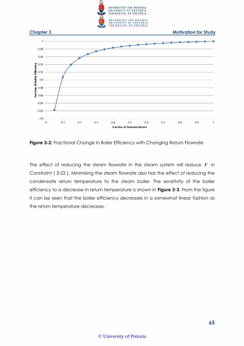
Chapter 3 Motivation for Study
65
Figure 3-2: Fractional Change in Boiler Efficiency with Changing Return Flowrate
The effect of reducing the steam flowrate in the steam system will reduce F in
Constraint ( 3-22 ). Minimising the steam flowrate also has the effect of reducing the
condensate return temperature to the steam boiler. The sensitivity of the boiler
efficiency to a decrease in return temperature is shown in Figure 3-3. From the figure
it can be seen that the boiler efficiency decreases in a somewhat linear fashion as
the return temperature decreases.
© University of Pretoria
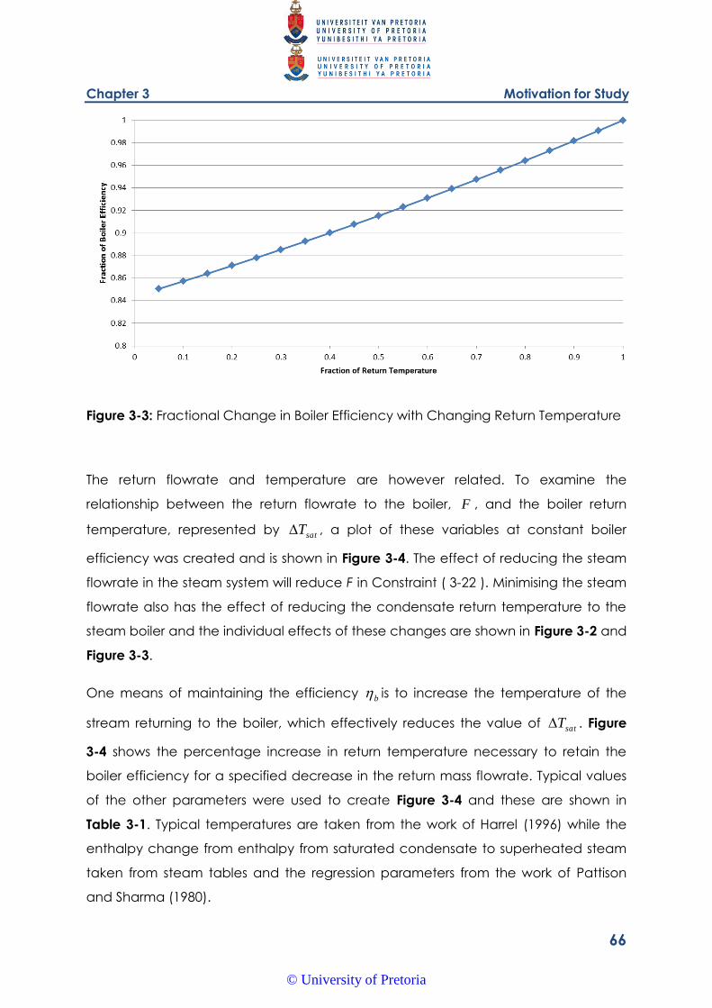
Chapter 3 Motivation for Study
66
Figure 3-3: Fractional Change in Boiler Efficiency with Changing Return Temperature
The return flowrate and temperature are however related. To examine the
relationship between the return flowrate to the boiler, F , and the boiler return
temperature, represented by satT , a plot of these variables at constant boiler
efficiency was created and is shown in Figure 3-4. The effect of reducing the steam
flowrate in the steam system will reduce F in Constraint ( 3-22 ). Minimising the steam
flowrate also has the effect of reducing the condensate return temperature to the
steam boiler and the individual effects of these changes are shown in Figure 3-2 and
Figure 3-3.
One means of maintaining the efficiency b is to increase the temperature of the
stream returning to the boiler, which effectively reduces the value of satT . Figure
3-4 shows the percentage increase in return temperature necessary to retain the
boiler efficiency for a specified decrease in the return mass flowrate. Typical values
of the other parameters were used to create Figure 3-4 and these are shown in
Table 3-1. Typical temperatures are taken from the work of Harrel (1996) while the
enthalpy change from enthalpy from saturated condensate to superheated steam
taken from steam tables and the regression parameters from the work of Pattison
and Sharma (1980).
© University of Pretoria
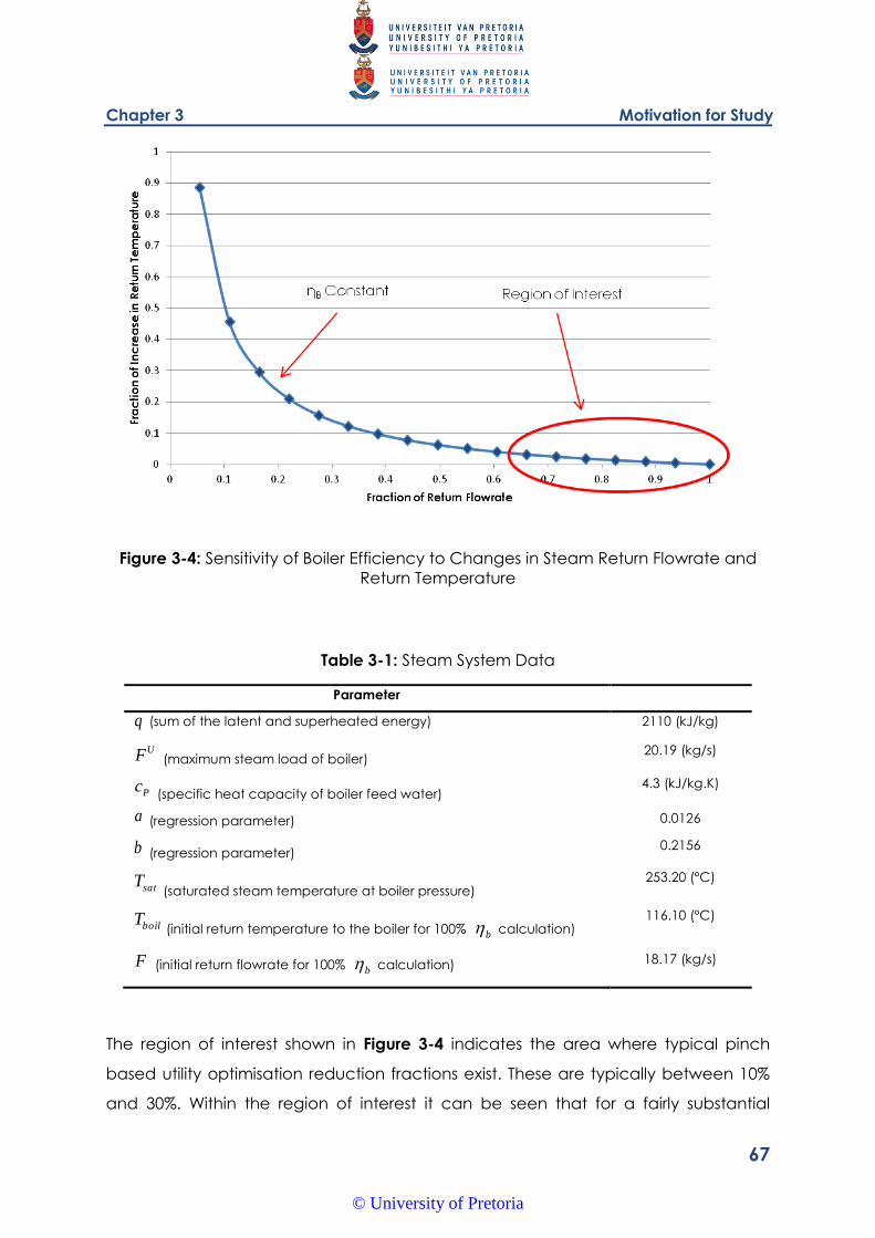
Chapter 3 Motivation for Study
67
Figure 3-4: Sensitivity of Boiler Efficiency to Changes in Steam Return Flowrate and
Return Temperature
Table 3-1: Steam System Data
Parameter
q (sum of the latent and superheated energy) 2110 (kJ/kg)
UF (maximum steam load of boiler) 20.19 (kg/s)
Pc (specific heat capacity of boiler feed water)
4.3 (kJ/kg.K)
a (regression parameter) 0.0126
b (regression parameter) 0.2156
satT (saturated steam temperature at boiler pressure)
253.20 (°C)
boilT (initial return temperature to the boiler for 100% b calculation)
116.10 (°C)
F (initial return flowrate for 100% b calculation) 18.17 (kg/s)
The region of interest shown in Figure 3-4 indicates the area where typical pinch
based utility optimisation reduction fractions exist. These are typically between 10%
and 30%. Within the region of interest it can be seen that for a fairly substantial
© University of Pretoria
Chapter 3 Motivation for Study
68
decrease in return flowrate a relatively small increase in the return temperature is
required to maintain the efficiency defined by Constraint ( 3-22 ).
Maintaining the boiler efficiency during a debottlenecking exercise remains a
brownfields application as newer steam systems may be designed with heat
integration considered.
3.5. Optimality of Flow Solutions in Network Optimisation Problems
The advent of pinch techniques in the design and optimisation of heat and mass
exchange networks gave process designers a systematic tool to reduce utility
consumption. Many of the techniques described by Linnhoff and Hindmarsh (1982)
are still used as the basis of utility stream design and optimisation.
Heat and mass exchange networks, and the optimisation of these networks share
several common features. These include, but are not limited to:
The requirement for a driving force to transfer so called units of interest (heat
or the mass of a particular component);
The use of a medium to transfer units of interest; and
The requirement to create products of the flow medium and the unit of
interest so as to achieve the objective of interest (heating duty or mass load).
The last point brings with it the difficulty of variable product bilinear terms in
optimisation. These terms are nonconvex and present difficulties for MINLP solvers.
In most heat and mass exchange network optimisation formulations the mass
balance elements of the transfer medium are simple and are based around a
superstructure. The constraints derived from this superstructure are typically linear.
The inclusion of heat and mass transfer constraints are typically accompanied by
bilinear terms as described above, making the formulation nonlinear. Formulations
based around a generic superstructure also typically contain binary variables to
denote the existence of streams and units and therefore the resulting heat or mass
exchange optimisation problem is presented as an MINLP.
© University of Pretoria
Chapter 3 Motivation for Study
69
Savelski and Bagajewicz (2000) began investigating the nature of the concentration
of streams leaving mass exchange units in wastewater minimisation problems. Initially
with single contaminants, the authors derived a proof whereby if the outlet
concentration of the stream leaving a mass exchange unit was set to its maximum,
the minimum wastewater flowrate could be realised by the system. Also, as the
outlet concentration limits are fixed values, their inclusion transformed the nonlinear
mass exchange constraints of the formulation to linear constraints. The wastewater
minimisation problem could therefore be presented as an MILP. The authors
expanded this theorem to include multiple contaminants and presented the proofs
and formulation in Savelski and Bagajewicz (2003).
A parallel to this work can be drawn to heat exchange networks and the
minimisation of cooling water or steam. Coetzee and Majozi (2008) utilised this
technique to minimise the steam flowrate to HENs by the recycle and reuse of hot
condensate.
3.5.1. Degenerate Solutions
Savelski and Bagajewicz (2000) identify that multiple solution networks exist when
solving wastewater minimisation problems using the condition of maximum outlet
concentration. They further describe how optimal mass flowrate solutions can exist
where the maximum outlet concentrations are not met. These network solutions are
termed degenerate solutions by the authors, who describe manual iterative solution
technique to find such solutions. The authors do however point out how the
degenerate solutions can be used to optimise a further network variable, such as the
number of flow connections, while still achieving the minimum fresh water intake.
The primary drawback to using degenerate solutions to further optimise flow
networks is the bilinear terms which need to be solved. These bilinear terms are
nonlinear and nonconvex, which, as will be shown in Section 3.6, present severe
difficulties to MINLP solvers.
© University of Pretoria
Chapter 3 Motivation for Study
70
3.6. Branch and Bound MINLP Solvers
A wide variety of MINLP solvers have been developed in the last few decades. Those
stemming from the work of Kelley (1960) tend to exhibit a linearisation step which is
used to create an MILP master problem in conjunction with non linear sub problems.
These solvers include BARON by Sahinidis and Tawamalani (2005), DICOPT by
Grossmann et al. (2005) and alphaECP by Westerlund and Pettersson (1995). These
solvers utilise an iterative search procedure which fixes binary variables and solves
NLP sub problems and thereafter uses the solution to the NLP sub problem to create
linearisations of nonlinear constraints to form an MILP master problem. The solvers
vary in how the various NLP solutions and their linearised solutions, often referred to
as integer cuts, are used. A very generic solution diagram is shown in Figure 2-1.
© University of Pretoria
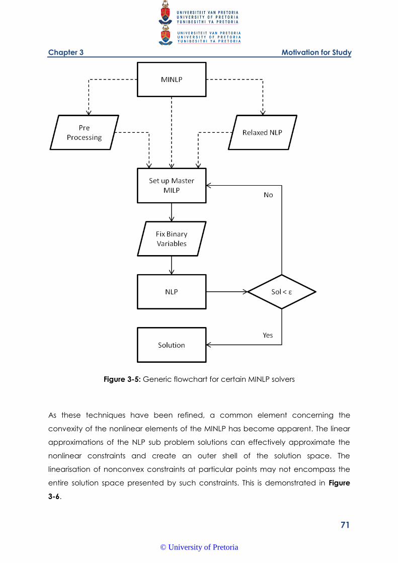
Chapter 3 Motivation for Study
71
Figure 3-5: Generic flowchart for certain MINLP solvers
As these techniques have been refined, a common element concerning the
convexity of the nonlinear elements of the MINLP has become apparent. The linear
approximations of the NLP sub problem solutions can effectively approximate the
nonlinear constraints and create an outer shell of the solution space. The
linearisation of nonconvex constraints at particular points may not encompass the
entire solution space presented by such constraints. This is demonstrated in Figure
3-6.
© University of Pretoria
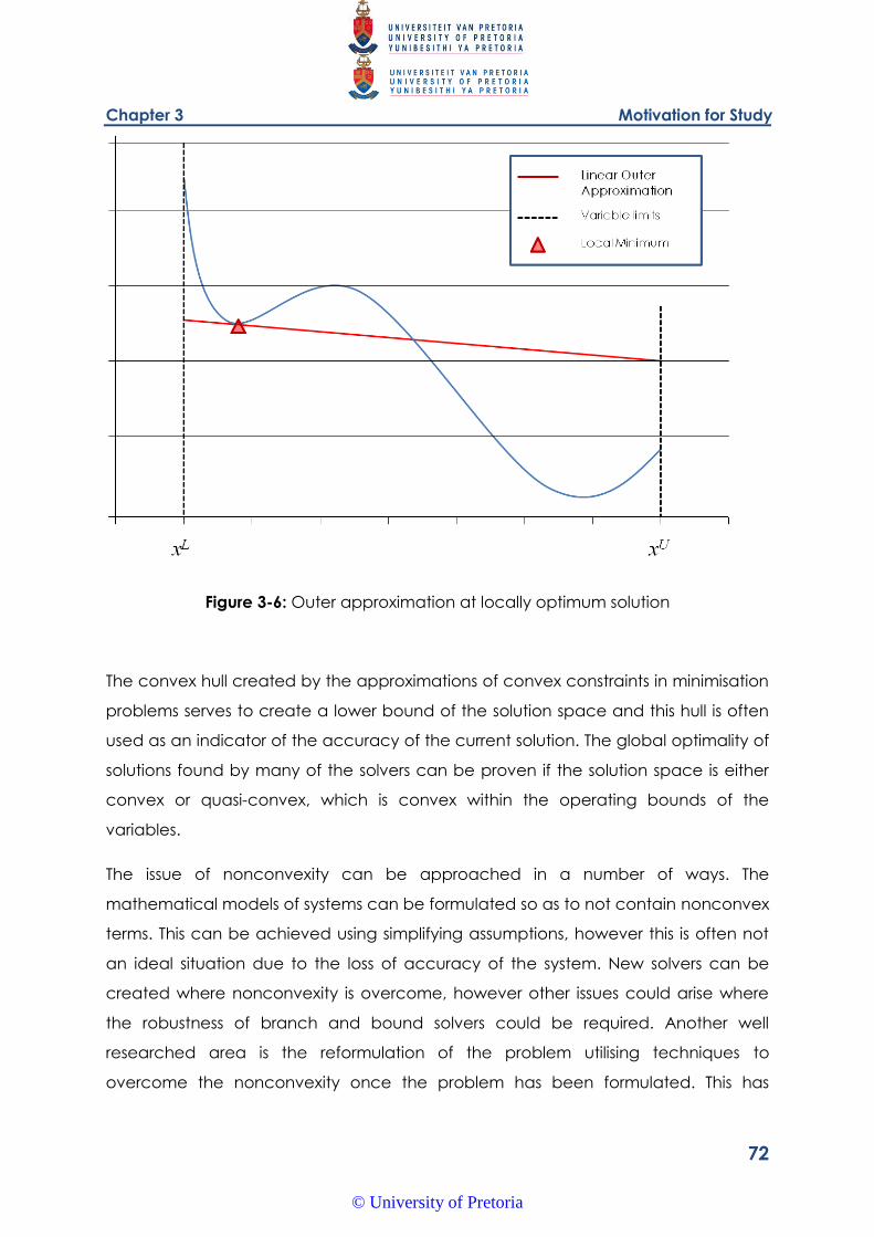
Chapter 3 Motivation for Study
72
Figure 3-6: Outer approximation at locally optimum solution
The convex hull created by the approximations of convex constraints in minimisation
problems serves to create a lower bound of the solution space and this hull is often
used as an indicator of the accuracy of the current solution. The global optimality of
solutions found by many of the solvers can be proven if the solution space is either
convex or quasi-convex, which is convex within the operating bounds of the
variables.
The issue of nonconvexity can be approached in a number of ways. The
mathematical models of systems can be formulated so as to not contain nonconvex
terms. This can be achieved using simplifying assumptions, however this is often not
an ideal situation due to the loss of accuracy of the system. New solvers can be
created where nonconvexity is overcome, however other issues could arise where
the robustness of branch and bound solvers could be required. Another well
researched area is the reformulation of the problem utilising techniques to
overcome the nonconvexity once the problem has been formulated. This has
© University of Pretoria
Chapter 3 Motivation for Study
73
proven effective at allowing the branch and bound solvers to overcome the
problem. Some of these techniques are mentioned below.
3.6.1. Techniques to Overcome Bilinear Terms and Nonconvexity
To utilise the degenerate solutions described in Section 3.5.1 above, a means to deal
with bilinear terms will be needed. A well established technique, which has been
used to the predecessor of this work by Price and Majozi (2010a), is the relaxation
and linearisation technique of Sherali and Alameddine (1992) which was utilised very
successfully be Quesada and Grossmann (1995). A large amount of research has
also been conducted into the convexification of nonconvex, nonlinear terms in
order to find optimal solutions for difficult MINLP problems. This work culminated in a
technique described by Pörn, et al. (2008), where transformations are used to alter
the nonconvex polynomial terms. Bilinear terms are a special, simpler variety of
polynomials. Therefore this technique shows great potential to deal with the bilinear
terms formed by the degenerate solutions described by Savelski and Bagajewicz
(2000).
Relaxation and Linearisation
Quesada and Grossmann (1995) investigate systems of mixers, splitters and process
units where multi-component streams vary in flow and composition. The authors
identify the complexity of bilinear terms created by products of wither the flow and
concentration variables of the streams or the flow and composition fraction
variables of the streams. The authors present an efficient global optimisation
methodology termed reformulation and linearisation. This method is based on
concave and convex envelopes formed from the bounds of the variables
constituting the bilinear term. This method was first described by McCormick (1976)
and first proposed for use of reformulation and linearisation by Sherali and
Alameddine (1992). The authors utilise this technique to remove the nonlinear,
nonconvex bilinear terms and replace them with single variables whose bounds are
formulated from the bounds of the individual variables in the bilinear terms. This
effectively linearises the composition and flow bilinear terms and helps prevent
solutions becoming trapped in sub optimal solutions and convergence failures of
NLP problems. The linearised model also creates an effective lower bound for the
© University of Pretoria
Chapter 3 Motivation for Study
74
optimisation problem. The authors then develop a branch and bound technique to
cater for binary terms often found in process stream optimisation problems. The
technique is successfully demonstrated on a number of test problems.
Price and Majozi (2010a) utilised the reformulation and linearisation technique to
eliminate bilinear terms in their work to reduce steam consumption in HENs and
maintain boiler efficiency. The authors used this technique to create a linearised
MILP model where the solution would be the starting point of an exact MINLP model.
Global optimality can be proven if the solution to the exact model is equivalent to
the solution to the relaxed model.
Transformation and Convexification
Westerlund and co-workers describe conditions of convexity and make large strides
to transform various kinds of nonconvex, nonlinear terms into convex terms. The
techniques developed focus on a transformation of the nonconvex terms into
convex terms. The sign of the nonconvex terms dictate which transformation is
utilised. Pörn et al.(1999)first describe the Exponential Transform (ET) or the Inverse
Transform (IT) for positively signed terms as well as the Potential Transform (PT) for
negatively signed terms.
The convexification principle is based on the fact that positive logarithmic and
inverse functions are convex when positive while negative inverse power functions
are convex in the positive variable space. A transformation variable is created for
each convexification. This transformation variable is consequently also nonlinear and
nonconvex, however this variable appears individually in constraints and can more
easily be approximated with piecewise approximations. Pörn et al. (1999) discuss
different convexification techniques for various classes of nonconvex posynomial
functions. The authors present the Exponential Transform (ET) as well as the Potential
Transform (PT) which are used to transform positively and negatively signed
posynomial terms into convex terms respectively. The transformations take
advantage of certain convex functions, exponential and power functions, and
transform nonconvex functions such that the convex exponential and power
functions may be used in the formulation. Pörn et al, (2008) present a more general
transformation strategy for functions with signomial terms. The authors further suggest
© University of Pretoria
Chapter 3 Motivation for Study
75
the use piecewise linear approximations to handle the nonconvex constraints
resulting from the transformation of signomial terms. The authors present a systematic
solution strategy for the convexification and optimisation of MINLP problems which
contain nonconvex signomial terms.
This technique can be used to transform signomial terms into convex terms and if a
solution is found it can be proved to be a globally optimal solution. This feature
could make this technique favourable as bilinear terms frequently cause locally
optimal solutions.
3.6.2. Application in Degenerate Flow Network Problems
If the flowrate minimisation model of Coetzee and Majozi (2008) is examined, a
nonlinear, nonconvex constraint is identified as the energy constraint describing the
sensible heat transfer from the condensate streams to the process streams. Coetzee
and Majozi (2008) utilise the optimality conditions described by Savelski and
Bagajewicz (2000) to overcome these nonlinearities and create an MILP formulation
which is subsequently solved to optimality.
As the formulation of Coetzee and Majozi (2008) is linear, there are multiple network
configurations which exhibit the minimum steam flowrate. These networks can
therefore be optimised for another design variable while still achieving the minimum
steam flowrate. Price and Majozi (2010c) use this methodology to minimise the
network pressure drop for the system while maintaining the minimum steam flowrate.
This work will be examined in Chapter 4.
As discussed in Section 3.5.1, if the optimality conditions of Savelski and Bagajewicz
(2000) are removed from a network system, the minimum flowrate through the
system can still be achieved. Therefore it follows that these degenerate solutions
should be examined in an attempt to find better secondary objectives for the
networks, such as a better minimum system pressure drop. The formulation of Price
and Majozi (2010c) will be further examined for this purpose.
The sensible heat transfer constraint defined by Coetzee and Majozi (2008) and also
used by Price and Majozi (2010c) contains three bilinear terms. The difficulty in
finding the network which minimises system pressure drop as well as achieves the
© University of Pretoria
Chapter 3 Motivation for Study
76
minimum steam flowrate through the system is in solving an MINLP formulation which
contains bilinear as well as other nonlinear terms. In accordance with the conditions
described by Westerlund et al. (2011) the bilinear terms are not only nonlinear but
also nonconvex. The bilinear terms appear in the same constraint which is binding as
the energy requirements of the process streams heated by the network need to be
met.
In addition the formulation contains nonlinear terms to represent pressure drop as a
function of the mass flowrate of steam and condensate. The formulation also
contains binary variables which necessitate the use of an MINLP solver.
3.6.3. Solution Process
The solution process will therefore need to focus on handling the bilinear terms as
well as being considerate of the workings of the MINLP solvers for complex problems.
The relaxation and convexification techniques discussed in Section 3.6.1 show
promise for handling the bilinear terms while a number of other techniques are
advised by the authors of the MINLP solvers themselves.
Therefore the solution process performed by Price and Majozi (2010a) as well as
Price and Majozi (2010c) will be reviewed and where possible improved upon, while
a solution algorithm specific to further optimising network problems using
degenerate flow solutions will be proposed.
Initially the solution process will focus on steam system heat exchanger network
pressure drop, however the steam system boiler efficiency will also be examined.
3.7. References
Adekola, O, Stamp, J. D, Majozi, T, Garg, A. and Bandyopadhyay, S. (2013) Unified
Approach for the Optimization of Energy and Water in Multipurpose Batch Plants
Using a Flexible Scheduling Framework, Industrial Engineering Chemistry Research
2013, 52, 8488-8506.
© University of Pretoria
Chapter 3 Motivation for Study
77
Beangstrom, S. G. and Majozi, T. (2012) A Process Integration Technique for Steam
System Synthesis Involving Multiple Levels, Computer Aided Chemical Engineering
2012, 31, 460-464.
Coetzee, W.A. and Majozi, T. (2008) Steam System Network Design Using Process
Integration, Industrial Engineering Chemistry Research 2008, 47, 4405-4413.
Frank, O. (1978) Simplified design procedure for tubular exchangers, Practical
aspects of heat transfer, Chem. Eng. Prog. Tech. Manual (Am. Inst. Chem. Eng).
Gass, S. I. (1985) Linear Programming, 5th Edition, Mcgraw-Hill, New York.
Glover, F. (1975) Improved linear integer programming formulation of nonlinear
problems, Management Science, Pages 455-460.
Gololo, K. V. and Majozi, T. (2011), On Synthesis and Optimization of Cooling Water
Systems with Multiple Cooling Towers, Industrial Engineering Chemistry Research
2011, 50 (7), 3775−3787.
Gololo, K. V. and Majozi, T. (2013) Complex Cooling Water Systems Optimization with
Pressure Drop Consideration, Industrial Engineering Chemistry Research 2013, 52,
7056−7065.
Grossmann, I. E. Viswanathan, J. Vecchietti, A. Raman, R. and Kalvelagen, E. (2005).
DICOPT A Discrete Continuous Optimization Package. In GAMS The Solver Manuals
(pp. 147-166). Washington: GAMS Development Corporation.
Hewit, G. F, Spires, G. L. and Bott, T. R. (1994) Process Heat Transfer, CRC Press.
Kelley, J. E. (1960) The Cutting Plane Method for Solving Convex Programs, Journal of
the SIAM 1960, 8, 703–712.
Kern, D. Q. (1950) Process heat transfer, Mcgraw Hill, New York.
Kim, J. K. and Smith, R. (2003) Automated retrofit design of cooling-water systems,
Process Systems Engineering, Vol 49, No7, pages 1712-1730.
Linnhoff, B. and Hindmarsh, E. (1982) The Pinch method for heat exchanger network,
Chemical Engineering Science, Vol 38, No 5, pages 745-763.
© University of Pretoria
Chapter 3 Motivation for Study
78
Majozi, T. and Moodley, A. (2008) Simultaneous targeting and design for cooling
water systems with multiple cooling water supplies, Computers and Chemical
Engineering, Vol 32, pages 540-551.
Majozi, T. and Nyathi, N. (2007), On Cooling-water Systems Design for South African
Industry: Two Recent Developments, South African Journal of Science 2007, 103, 239-
244.
McCormick, G. (1976) Computability of global solutions to factorable nonconvex
programs. Part I Convex underestimating problems.
Ndlovu, M. and Majozi, T. (2014) Design and Optimisation of Power Plant Utility
Systems, Computer Aided Chemical Engineering 2014, 34, 567-572.
Nie, X. R. (1998) Heat exchanger network retrofit considering pressure drop and heat
transfer enhancement, Ph.D. Thesis, UMIST, Manchester.
Nie, X. and Zhu, X. X. (2002) Pressure drop considerations for heat exchanger
grassroot design, Computers and Chemical Engineering, Vol 26, pages 1661-1676.
Pattison, J. R. and Sharma, V. (1980) Selection of boiler plant and overall system
efficiency, Studies in energy efficiency in buildings, British Gas.
Peters, M. S. and Timmerhaus, K. D. (1991) Plant design and economics for chemical
engineers, 4th Edition, Mcgraw-Hill, New York.
Pörn, R., Bjork, K., and Westerlund, T. (2008) Global solution of optimization problems
with signomial parts. Discrete Optimization 5 , 108-120.
Pörn, R. Harjunkoski, I. and Westerlund, T. (1999) Convexification of different classes of
non-convex MINLP problems. Computers and Chemical Engineering 23 , 439-448.
Price, T. and Majozi, T. (2010a) On Synthesis and Optimization of Steam System
Networks. 1. Sustained Boiler Efficiency. Industrial Engineering Chemistry Research 49
, 9143–9153.
Price, T. and Majozi, T. (2010b) Synthesis and Optimization of Steam System Networks.
2. Multiple Steam Levels. Industrial Engineering Chemistry Research 49 , 9154–9164.
© University of Pretoria
Chapter 3 Motivation for Study
79
Price, T. and Majozi, T. (2010c) On Synthesis and Optimization of Steam System
Networks. 3. Pressure Drop Consideration. Industrial Engineering Chemistry Research
49 , 9165–9174.
Quesada, I. and Grossmann, I. E. (1995) Global optimisation of bilinear process
networks with multi component flows, Computers and Chemical Engineering 19, No
12, pages 1219-1242.
Sahinidis, N. and Tawamalani, M. (2005) BARON. In GAMS The Solver Manuals (pp. 9-
22). Washington: GAMS Develpoment Corporation.
Savelski, M. J. and Bagajewicz, M. J. (2000) On the optimality conditions of water
utilization systems in process plants with single contaminants, Chemical Engineering
Science 55, pages 5035-5048.
Savelski, M. J. and Bagajewicz, M. J. (2003) On the necessary conditions of optimality
of water utilization systems in process plants with multiple contaminants. Chemical
Engineering Science , 58, 5349-5362.
Seid, E. R. and Majozi, T (2014), Heat Integration in Multipurpose Batch Plants Using a
Robust Scheduling Framework, Energy 2014, 71, 302-320.
Shang, Z. and Kokossis, A. (2004) A transhipment model for the optimisation of steam
levels of total site utility system for multiperiod operation, Computers and Chemical
Engineering 28, pages 1673-1688.
Sherali, H. D. and Alameddine, A. (1992). A New Reformulation-
LinearizationTechnique for Bilinear Programming Problems. Journal of Global
Optimization , 2, 379-410.
Sinnot, R. K. (2005) Chemical engineering design, Vol 6, Elsevier Butterworth
Heinemann, New York.
Stamp, J. and Majozi, T. (2011) Optimum Heat Storage Design for Heat Integrated
Multipurpose Batch Plants, Energy 2011, 36, 5119-5131.
Westerlund, T. and Pettersson, F. (1995). An Extended Cutting Plane Method for
Solving Convex MINLP Problems. Computers and Chemical Engineering 19 , 131-136.
© University of Pretoria
Chapter 3 Motivation for Study
80
Zhelev, T, Semkov, K, Mooney, E, Majozi, T. and Korobeinikov, A. (2013) Industrial Heat
Utilization Through Water Management, Heat Transfer Engineering 2013, 34, 1191-
1201.
© University of Pretoria
Chapter 4 Model Formulation
81
4. Model Formulation
This chapter is intended to present all models formulated for this thesis. The models
are largely based on the flow minimisation model of Coetzee and Majozi (2008) as
well as the steam system network pressure drop model of Price and Majozi (2010c)
and the single supply steam pressure boiler efficiency optimisation model of Price
and Majozi (2010a). These models will be presented first and then where necessary
areas will be expanded upon.
The chapter will first investigate the basic flow minimisation model as well as some
techniques used to simplify the formulation. The basic network pressure drop model
which includes condensers will be presented next, followed by the alterations
needed to solve the flow minimisation model for degenerate solutions as well as
techniques used to simplify this formulation. Two solution techniques have been
explored to solve the degenerate solution MINLP problem and these will be
presented, along with any simplification techniques that are applicable. Lastly this
chapter will apply the techniques discussed above to an additional area of HEN
optimisation, namely boiler efficiency.
4.1. Flow Minimisation Constraints
This section shows the flow minimisation model as well as solution techniques directly
associated with it.
4.1.1. Steam System Heat Exchanger Network Flow Minimisation Constraints
Figure 4-1 shows the superstructure used by Coetzee and Majozi (2008) to represent
a system where steam and condensate are used to provide heat to a HEN. Referring
to Figure 4-1, FS is the total flowrate of saturated steam from the boiler. Each heat
exchanger, represented by i or j in the figure, can receive saturated steam or
recycled/reused condensate, represented in the figure by SS and FRR
respectively. The outlet from each heat exchanger can be saturated or subcooled
condensate, depending on the nature of the inlet stream. The same outlet stream
© University of Pretoria
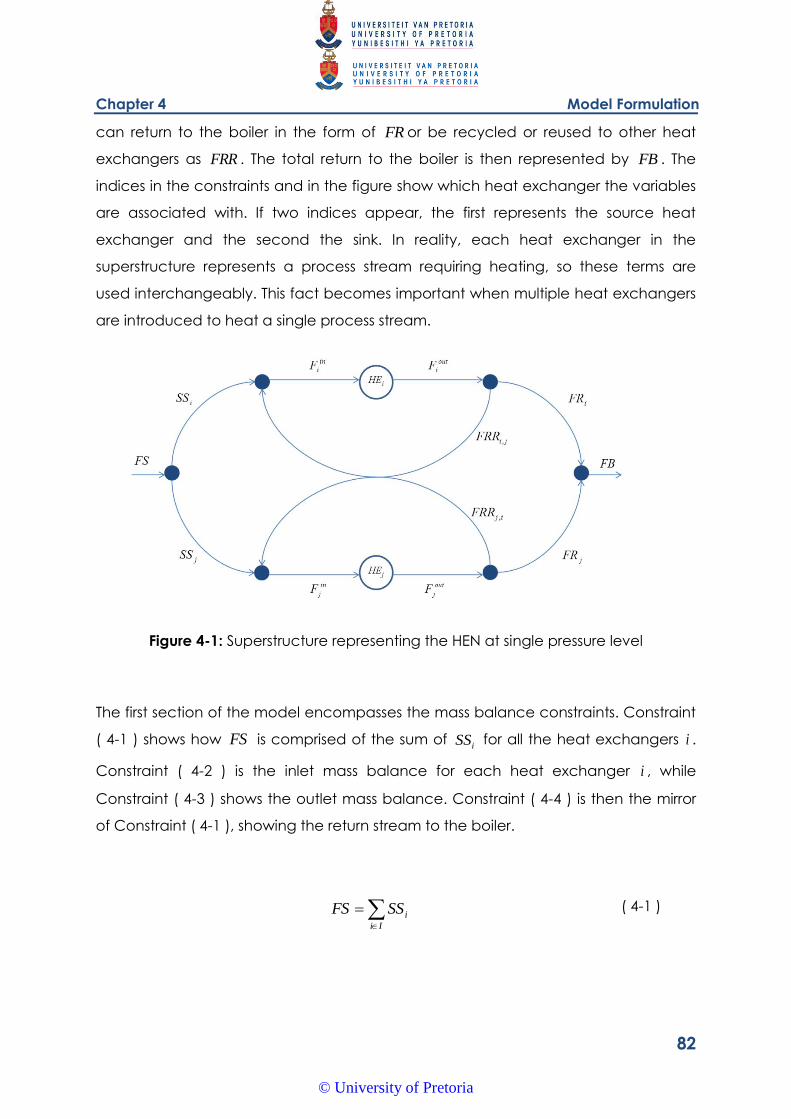
Chapter 4 Model Formulation
82
can return to the boiler in the form of FR or be recycled or reused to other heat
exchangers as FRR . The total return to the boiler is then represented by FB . The
indices in the constraints and in the figure show which heat exchanger the variables
are associated with. If two indices appear, the first represents the source heat
exchanger and the second the sink. In reality, each heat exchanger in the
superstructure represents a process stream requiring heating, so these terms are
used interchangeably. This fact becomes important when multiple heat exchangers
are introduced to heat a single process stream.
Figure 4-1: Superstructure representing the HEN at single pressure level
The first section of the model encompasses the mass balance constraints. Constraint
( 4-1 ) shows how FS is comprised of the sum of iSS for all the heat exchangers i .
Constraint ( 4-2 ) is the inlet mass balance for each heat exchanger i , while
Constraint ( 4-3 ) shows the outlet mass balance. Constraint ( 4-4 ) is then the mirror
of Constraint ( 4-1 ), showing the return stream to the boiler.
Ii
iSSFS ( 4-1 )
© University of Pretoria
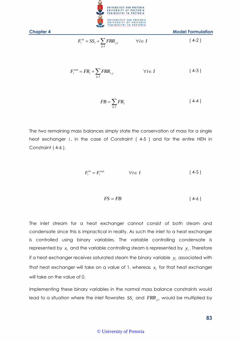
Chapter 4 Model Formulation
83
IiFRRSSFIj
iji
in
i
, ( 4-2 )
IiFRRFRFIj
jii
out
i
, ( 4-3 )
Ii
iFRFB ( 4-4 )
The two remaining mass balances simply state the conservation of mass for a single
heat exchanger i , in the case of Constraint ( 4-5 ) and for the entire HEN in
Constraint ( 4-6 ).
IiFF out
i
in
i ( 4-5 )
FBFS ( 4-6 )
The inlet stream for a heat exchanger cannot consist of both steam and
condensate since this is impractical in reality. As such the inlet to a heat exchanger
is controlled using binary variables. The variable controlling condensate is
represented by ix and the variable controlling steam is represented by
iy . Therefore
if a heat exchanger receives saturated steam the binary variable iy associated with
that heat exchanger will take on a value of 1, whereas ix for that heat exchanger
will take on the value of 0.
Implementing these binary variables in the normal mass balance constraints would
lead to a situation where the inlet flowrates iSS and ijFRR , would be multiplied by
© University of Pretoria
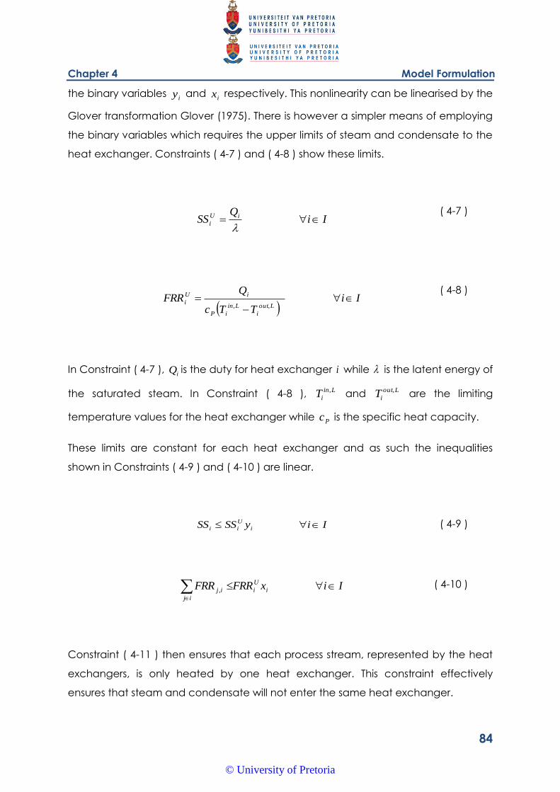
Chapter 4 Model Formulation
84
the binary variables iy and
ix respectively. This nonlinearity can be linearised by the
Glover transformation Glover (1975). There is however a simpler means of employing
the binary variables which requires the upper limits of steam and condensate to the
heat exchanger. Constraints ( 4-7 ) and ( 4-8 ) show these limits.
Ii
QSS iU
i
( 4-7 )
Ii
TTc
QFRR
Lout
i
Lin
iP
iU
i
,,
( 4-8 )
In Constraint ( 4-7 ), iQ is the duty for heat exchanger i while is the latent energy of
the saturated steam. In Constraint ( 4-8 ), Lin
iT , and
Lout
iT , are the limiting
temperature values for the heat exchanger while Pc is the specific heat capacity.
These limits are constant for each heat exchanger and as such the inequalities
shown in Constraints ( 4-9 ) and ( 4-10 ) are linear.
IiySSSS i
U
ii ( 4-9 )
IixFRRFRR i
U
i
ij
ij
, ( 4-10 )
Constraint ( 4-11 ) then ensures that each process stream, represented by the heat
exchangers, is only heated by one heat exchanger. This constraint effectively
ensures that steam and condensate will not enter the same heat exchanger.
© University of Pretoria
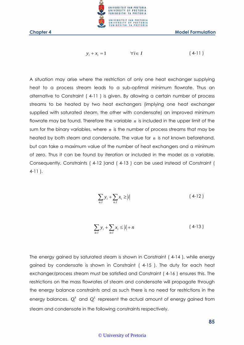
Chapter 4 Model Formulation
85
Iixy ii 1 ( 4-11 )
A situation may arise where the restriction of only one heat exchanger supplying
heat to a process stream leads to a sub-optimal minimum flowrate. Thus an
alternative to Constraint ( 4-11 ) is given. By allowing a certain number of process
streams to be heated by two heat exchangers (implying one heat exchanger
supplied with saturated steam, the other with condensate) an improved minimum
flowrate may be found. Therefore the variable n is included in the upper limit of the
sum for the binary variables, where n is the number of process streams that may be
heated by both steam and condensate. The value for n is not known beforehand,
but can take a maximum value of the number of heat exchangers and a minimum
of zero. Thus it can be found by iteration or included in the model as a variable.
Consequently, Constraints ( 4-12 )and ( 4-13 ) can be used instead of Constraint (
4-11 ).
ixyIi
i
Ii
i
( 4-12 )
nixyIi
i
Ii
i
( 4-13 )
The energy gained by saturated steam is shown in Constraint ( 4-14 ), while energy
gained by condensate is shown in Constraint ( 4-15 ). The duty for each heat
exchanger/process stream must be satisfied and Constraint ( 4-16 ) ensures this. The
restrictions on the mass flowrates of steam and condensate will propagate through
the energy balance constraints and as such there is no need for restrictions in the
energy balances. S
iQ and L
iQ represent the actual amount of energy gained from
steam and condensate in the following constraints respectively.
© University of Pretoria
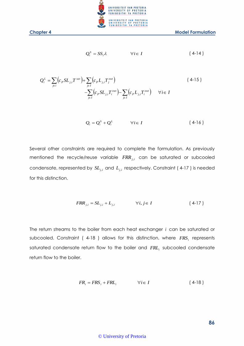
Chapter 4 Model Formulation
86
IiSSQ i
S
i ( 4-14 )
IiTLcTSLc
TLcTSLcQ
Ij
out
iijP
Ij
out
iijP
Ij
out
jijP
ij
sat
ijP
L
i
,,
,,
( 4-15 )
IiQQQ L
i
S
ii ( 4-16 )
Several other constraints are required to complete the formulation. As previously
mentioned the recycle/reuse variable ijFRR , can be saturated or subcooled
condensate, represented by ijSL , and ijL , respectively. Constraint ( 4-17 ) is needed
for this distinction.
IjiLSLFRR ijijij ,,,, ( 4-17 )
The return streams to the boiler from each heat exchanger i can be saturated or
subcooled. Constraint ( 4-18 ) allows for this distinction, where iFRS represents
saturated condensate return flow to the boiler and iFRL subcooled condensate
return flow to the boiler.
IiFRLFRSFR iii ( 4-18 )
© University of Pretoria
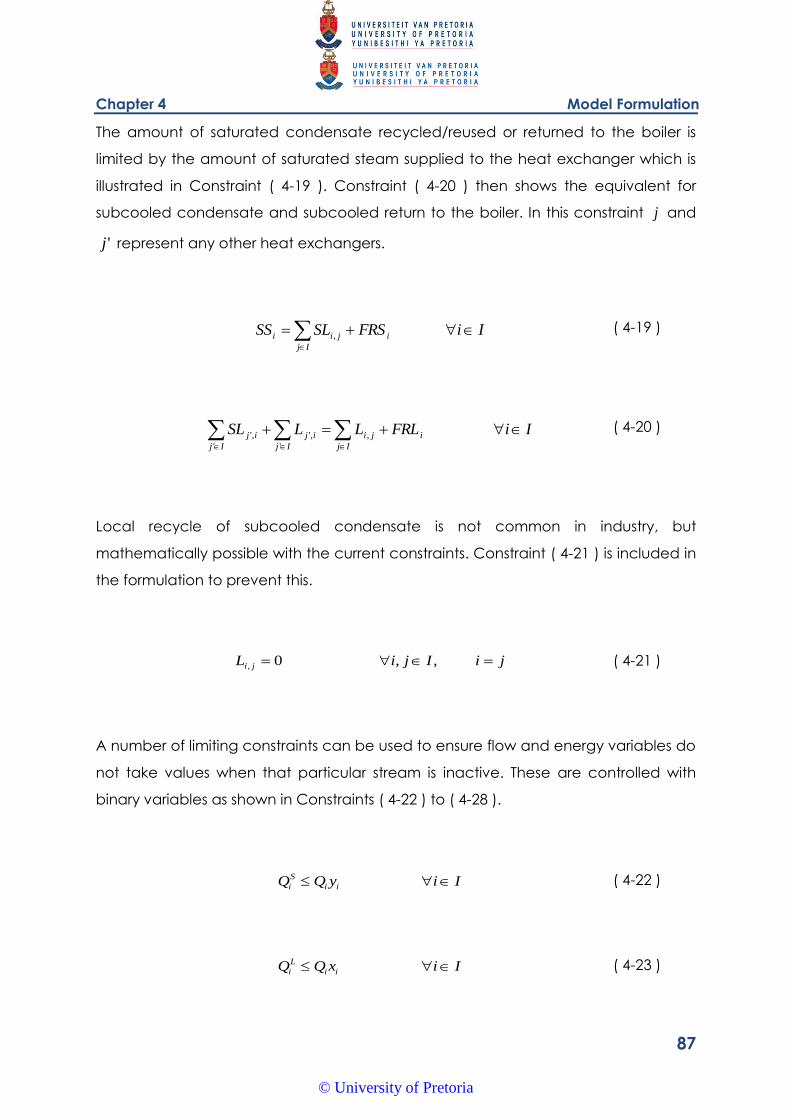
Chapter 4 Model Formulation
87
The amount of saturated condensate recycled/reused or returned to the boiler is
limited by the amount of saturated steam supplied to the heat exchanger which is
illustrated in Constraint ( 4-19 ). Constraint ( 4-20 ) then shows the equivalent for
subcooled condensate and subcooled return to the boiler. In this constraint j and
'j represent any other heat exchangers.
IiFRSSLSS i
Ij
jii
, ( 4-19 )
IiFRLLLSL i
Ij
ji
Ij
ij
Ij
ij
,
'
,'
'
,' ( 4-20 )
Local recycle of subcooled condensate is not common in industry, but
mathematically possible with the current constraints. Constraint ( 4-21 ) is included in
the formulation to prevent this.
jiIjiL ji ,,0, ( 4-21 )
A number of limiting constraints can be used to ensure flow and energy variables do
not take values when that particular stream is inactive. These are controlled with
binary variables as shown in Constraints ( 4-22 ) to ( 4-28 ).
IiyQQ ii
S
i ( 4-22 )
IixQQ ii
L
i ( 4-23 )
© University of Pretoria
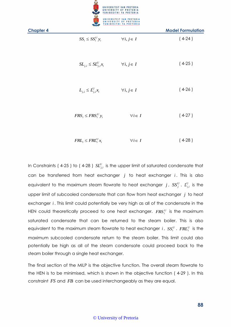
Chapter 4 Model Formulation
88
IjiySSSS i
U
ii , ( 4-24 )
IjixSLSL i
U
ijij ,,, ( 4-25 )
IjixLL i
U
ijij ,,, ( 4-26 )
IiyFRSFRS i
U
ii ( 4-27 )
IixFRLFRL i
U
ii ( 4-28 )
In Constraints ( 4-25 ) to ( 4-28 ) U
ijSL , is the upper limit of saturated condensate that
can be transferred from heat exchanger j to heat exchanger i . This is also
equivalent to the maximum steam flowrate to heat exchanger j , U
jSS . U
ijL , is the
upper limit of subcooled condensate that can flow from heat exchanger j to heat
exchanger i . This limit could potentially be very high as all of the condensate in the
HEN could theoretically proceed to one heat exchanger. U
iFRS is the maximum
saturated condensate that can be returned to the steam boiler. This is also
equivalent to the maximum steam flowrate to heat exchanger i , U
iSS . U
iFRL is the
maximum subcooled condensate return to the steam boiler. This limit could also
potentially be high as all of the steam condensate could proceed back to the
steam boiler through a single heat exchanger.
The final section of the MILP is the objective function. The overall steam flowrate to
the HEN is to be minimised, which is shown in the objective function ( 4-29 ). In this
constraint FS and FB can be used interchangeably as they are equal.
© University of Pretoria
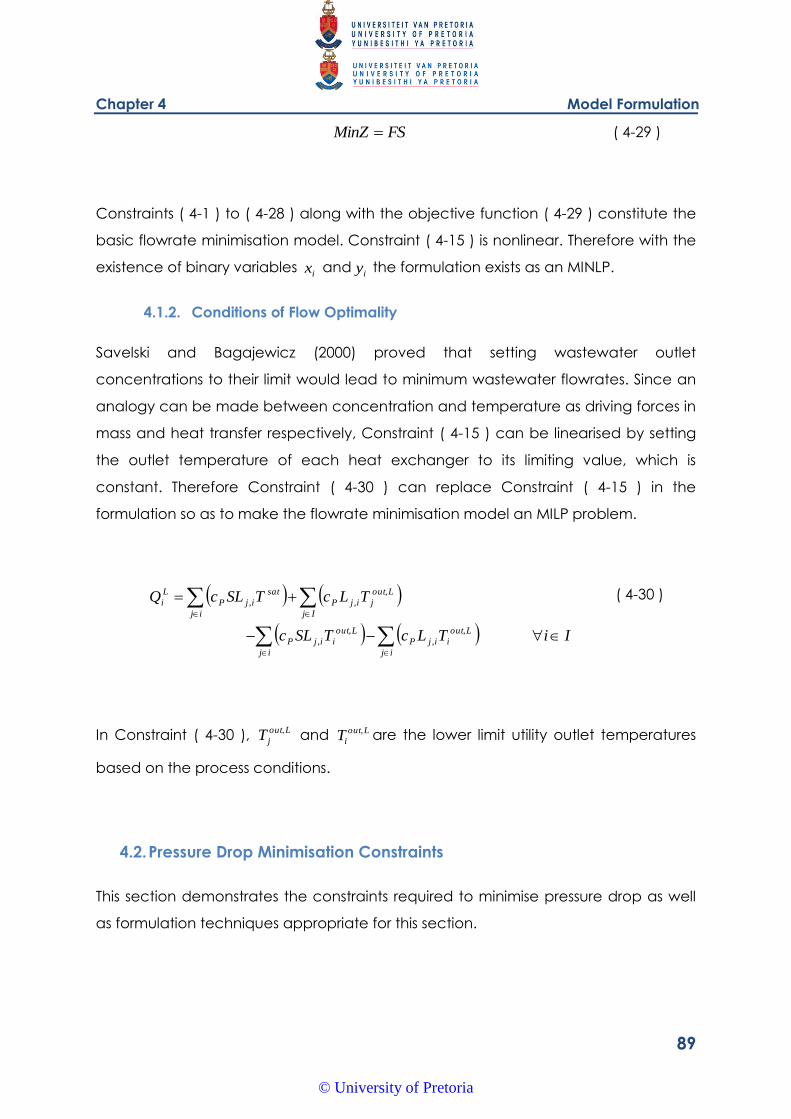
Chapter 4 Model Formulation
89
FSMinZ ( 4-29 )
Constraints ( 4-1 ) to ( 4-28 ) along with the objective function ( 4-29 ) constitute the
basic flowrate minimisation model. Constraint ( 4-15 ) is nonlinear. Therefore with the
existence of binary variables ix and
iy the formulation exists as an MINLP.
4.1.2. Conditions of Flow Optimality
Savelski and Bagajewicz (2000) proved that setting wastewater outlet
concentrations to their limit would lead to minimum wastewater flowrates. Since an
analogy can be made between concentration and temperature as driving forces in
mass and heat transfer respectively, Constraint ( 4-15 ) can be linearised by setting
the outlet temperature of each heat exchanger to its limiting value, which is
constant. Therefore Constraint ( 4-30 ) can replace Constraint ( 4-15 ) in the
formulation so as to make the flowrate minimisation model an MILP problem.
IiTLcTSLc
TLcTSLcQ
ij ij
Lout
iijP
Lout
iijP
Ij
Lout
jijP
ij
sat
ijP
L
i
,
,
,
,
,
,,
( 4-30 )
In Constraint ( 4-30 ), Lout
jT , and Lout
iT , are the lower limit utility outlet temperatures
based on the process conditions.
4.2. Pressure Drop Minimisation Constraints
This section demonstrates the constraints required to minimise pressure drop as well
as formulation techniques appropriate for this section.
© University of Pretoria
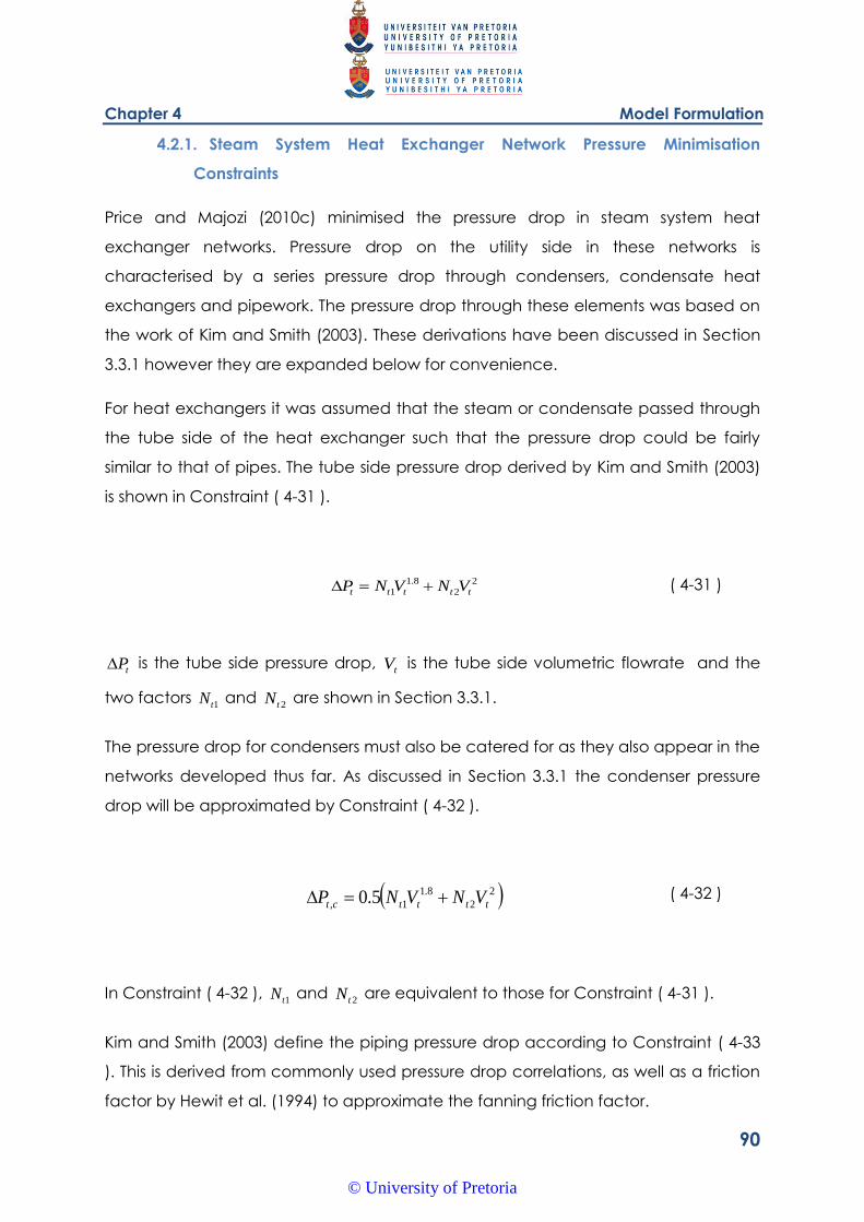
Chapter 4 Model Formulation
90
4.2.1. Steam System Heat Exchanger Network Pressure Minimisation
Constraints
Price and Majozi (2010c) minimised the pressure drop in steam system heat
exchanger networks. Pressure drop on the utility side in these networks is
characterised by a series pressure drop through condensers, condensate heat
exchangers and pipework. The pressure drop through these elements was based on
the work of Kim and Smith (2003). These derivations have been discussed in Section
3.3.1 however they are expanded below for convenience.
For heat exchangers it was assumed that the steam or condensate passed through
the tube side of the heat exchanger such that the pressure drop could be fairly
similar to that of pipes. The tube side pressure drop derived by Kim and Smith (2003)
is shown in Constraint ( 4-31 ).
2
2
8.1
1 ttttt VNVNP ( 4-31 )
tP is the tube side pressure drop, tV is the tube side volumetric flowrate and the
two factors 1tN and
2tN are shown in Section 3.3.1.
The pressure drop for condensers must also be catered for as they also appear in the
networks developed thus far. As discussed in Section 3.3.1 the condenser pressure
drop will be approximated by Constraint ( 4-32 ).
2
2
8.1
1, 5.0 ttttct VNVNP
( 4-32 )
In Constraint ( 4-32 ), 1tN and
2tN are equivalent to those for Constraint ( 4-31 ).
Kim and Smith (2003) define the piping pressure drop according to Constraint ( 4-33
). This is derived from commonly used pressure drop correlations, as well as a friction
factor by Hewit et al. (1994) to approximate the fanning friction factor.
© University of Pretoria
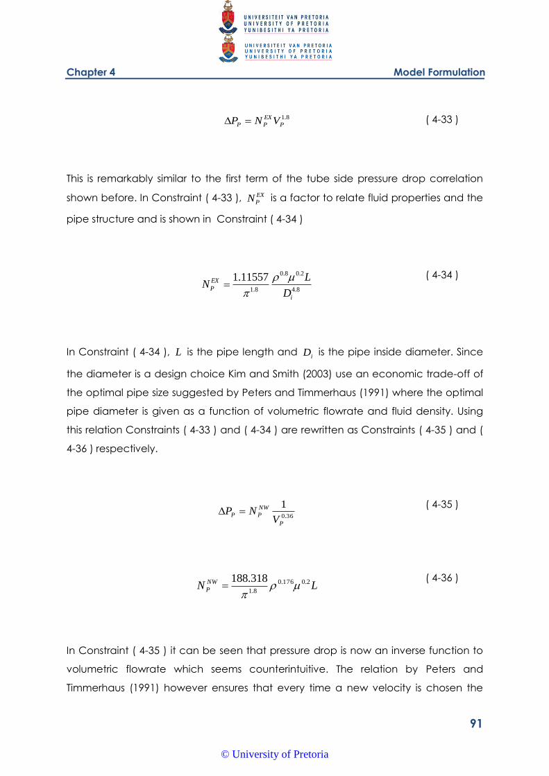
Chapter 4 Model Formulation
91
8.1
P
EX
PP VNP ( 4-33 )
This is remarkably similar to the first term of the tube side pressure drop correlation
shown before. In Constraint ( 4-33 ), EX
PN is a factor to relate fluid properties and the
pipe structure and is shown in Constraint ( 4-34 )
8.4
2.08.0
8.1
11557.1
i
EX
PD
LN
( 4-34 )
In Constraint ( 4-34 ), L is the pipe length and iD is the pipe inside diameter. Since
the diameter is a design choice Kim and Smith (2003) use an economic trade-off of
the optimal pipe size suggested by Peters and Timmerhaus (1991) where the optimal
pipe diameter is given as a function of volumetric flowrate and fluid density. Using
this relation Constraints ( 4-33 ) and ( 4-34 ) are rewritten as Constraints ( 4-35 ) and (
4-36 ) respectively.
36.0
1
P
NW
PPV
NP
( 4-35 )
LN NW
P
2.0176.0
8.1
318.188
( 4-36 )
In Constraint ( 4-35 ) it can be seen that pressure drop is now an inverse function to
volumetric flowrate which seems counterintuitive. The relation by Peters and
Timmerhaus (1991) however ensures that every time a new velocity is chosen the
© University of Pretoria
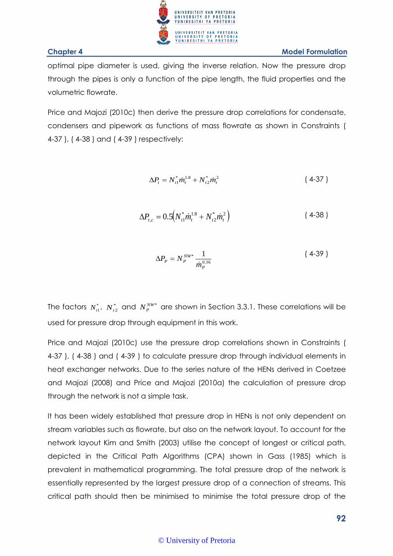
Chapter 4 Model Formulation
92
optimal pipe diameter is used, giving the inverse relation. Now the pressure drop
through the pipes is only a function of the pipe length, the fluid properties and the
volumetric flowrate.
Price and Majozi (2010c) then derive the pressure drop correlations for condensate,
condensers and pipework as functions of mass flowrate as shown in Constraints (
4-37 ), ( 4-38 ) and ( 4-39 ) respectively:
2*
2
8.1*
1 ttttt mNmNP
( 4-37 )
2*
2
8.1*
1, 5.0 ttttct mNmNP
( 4-38 )
36.0
* 1
P
NW
PPm
NP
( 4-39 )
The factors *
1tN , *
2tN and *NW
PN are shown in Section 3.3.1. These correlations will be
used for pressure drop through equipment in this work.
Price and Majozi (2010c) use the pressure drop correlations shown in Constraints (
4-37 ), ( 4-38 ) and ( 4-39 ) to calculate pressure drop through individual elements in
heat exchanger networks. Due to the series nature of the HENs derived in Coetzee
and Majozi (2008) and Price and Majozi (2010a) the calculation of pressure drop
through the network is not a simple task.
It has been widely established that pressure drop in HENs is not only dependent on
stream variables such as flowrate, but also on the network layout. To account for the
network layout Kim and Smith (2003) utilise the concept of longest or critical path,
depicted in the Critical Path Algorithms (CPA) shown in Gass (1985) which is
prevalent in mathematical programming. The total pressure drop of the network is
essentially represented by the largest pressure drop of a connection of streams. This
critical path should then be minimised to minimise the total pressure drop of the
© University of Pretoria
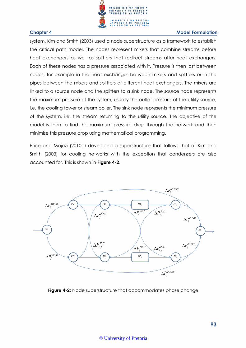
Chapter 4 Model Formulation
93
system. Kim and Smith (2003) used a node superstructure as a framework to establish
the critical path model. The nodes represent mixers that combine streams before
heat exchangers as well as splitters that redirect streams after heat exchangers.
Each of these nodes has a pressure associated with it. Pressure is then lost between
nodes, for example in the heat exchanger between mixers and splitters or in the
pipes between the mixers and splitters of different heat exchangers. The mixers are
linked to a source node and the splitters to a sink node. The source node represents
the maximum pressure of the system, usually the outlet pressure of the utility source,
i.e. the cooling tower or steam boiler. The sink node represents the minimum pressure
of the system, i.e. the stream returning to the utility source. The objective of the
model is then to find the maximum pressure drop through the network and then
minimise this pressure drop using mathematical programming.
Price and Majozi (2010c) developed a superstructure that follows that of Kim and
Smith (2003) for cooling networks with the exception that condensers are also
accounted for. This is shown in Figure 4-2.
Figure 4-2: Node superstructure that accommodates phase change
© University of Pretoria
Chapter 4 Model Formulation
94
In the figure it can be seen that the condensers are connected to the main source
node at source pressure PS . Since it is assumed that steam does not lose pressure in
pipes, SSHEP , is only as a result of the pressure drop in the condensers. The
distributing or splitting node after the condensers then has pressure PC . This node is
then connected to each condensate heat exchangers source node or mixer PB , as
well as the final sink node for return to the boiler PR . Since saturated condensate
exits the condensers, the pressure drop in the pipes between the PC and PB is a
function of the saturated condensate flowrate and the pressure drop is designated
SLPP , . It must also be noted that condensate can be reused by the same process
stream, and as such the SLP
iiP ,
, and SLP
jjP ,
, terms also exist. The direct return to the
boiler is accomplished by the saturated return flowrate FRS , thus this pressure drop
is designated FRSPP , .
The mixer node for each heat exchanger can also receive condensate from the
splitter nodes of other heat exchangers. This occurs in the form of subcooled liquid,
designated L , with associated pressure drop LPP , . The two condensate streams
then combine and pass through the heat exchanger. The pressure drop for each
heat exchanger is therefore a function of the sum of saturated and subcooled
condensate entering it. This is shown as LHEP , .
Finally each splitter node has the pressure PA . The return stream to the boiler, FRL ,
then proceeds to the return mixer with pressure PR . The pressure drop in the pipes of
this return stream is thus a function of this flowrate and is subsequently labelled
FRLPP , .
The method used by Kim and Smith (2003) based on the CPA to determine the
maximum pressure drop for the system is in the form of a difference in pressure
between nodes and the pressure drop between the nodes. This is represented in a
manner similar to Constraint ( 4-40 ) below.
BAPPBPA , ( 4-40 )
© University of Pretoria
Chapter 4 Model Formulation
95
In Constraint ( 4-40 ) it is understood that fluid flows from node A to node B . The
pressure difference between the nodes is essentially a result of the piping pressure
loss. Since the mixing nodes before a heat exchanger may receive fluid from
multiple sources, this constraint will occur several times with different source splitter
nodes and consequently different pressure drop values. The inequality in Constraint (
4-40 ) ensures that the PB assumes the lowest pressure value that satisfies all of the
constraints. In this way the node pressure is always at this low value when the model
is solved.
This constraint, though simple, is very elegant and effective at finding the critical
path, or in this case critical pressure drop for a given network. However, since it will
occur in the network design stage a means of eliminating those nodes that do not
exist must be made. Kim and Smith (2003) turned to binary variables to achieve this.
They established a connection existence binary variable for each connection in the
network. This binary variable takes the value of 1 if the connection exists and 0 if it
does not. An additional term is then added to Constraint ( 4-40 ) to render it
redundant for the cases where no connection exists. This is done by adding a large
pressure term BP such that it is satisfied for these cases. The large pressure is
represented by the term in Constraint ( 4-41 ).
BA
BA PyBPPBPA ,
,1 ( 4-41 )
The binary variables are created using the actual flow variables that are part of the
network design model and that are used to calculate the various pressure drops in
the model. The only nodes affected by this phenomenon are those that could
possibly receive multiple inputs. These are the PB and PR nodes, the mixers before
the condensate heat exchangers and the boiler return respectively. Only four flow
variables are associated with these and they are the saturated liquid flowrate
between heat exchangers ijSL ,, the subcooled liquid flowrate between streams
ijL ,,
the subcooled liquid flowrate to the boiler iFRL and the saturated liquid return
flowrate to the boiler iFRS . Each of the binary variables requires two constraints as
© University of Pretoria
Chapter 4 Model Formulation
96
well as known upper and lower bounds for the flowrates. Constraints ( 4-42 ) and (
4-43 ) are used to demonstrate this for the variable ijSL ,.
0,, SLU
ijij ySLSL ( 4-42 )
0,, SLL
ijij ySLSL ( 4-43 )
The binary variable will assume the correct value if the appropriate connection is
active. In Constraints ( 4-42 ) and ( 4-43 ), U
ijSL , and L
ijSL , are the upper and lower
limits respectively. Constraints ( 4-44 ) to ( 4-49 ) represent the longest path
constraints that exist according to the superstructure in Figure 4-2.
IiPPCPS SSHE
ii ,
( 4-44 )
IjiPyBPPBPC SLP
ij
SL
ijij ,1 ,
,, ( 4-45 )
IjiPyBPPBPA LP
ij
L
ijij ,1 ,
,, ( 4-46 )
IiPyBPPRPA FRLP
i
FRL
ii ,1
( 4-47 )
IiPyBPPRPC FRSP
i
FRS
ii ,1
( 4-48 )
© University of Pretoria
Chapter 4 Model Formulation
97
IiPPAPB LHE
iii , ( 4-49 )
The constraints shown above, as well as those showing the various pressure drops are
combined to form the pressure drop model. All that remains is to state the objective
function. Since the CPA finds the maximum pressure drop through the network, the
objective function then simply minimises this pressure drop. The objective function is
thus ( 4-50 ).
PRPSMinZ ( 4-50 )
A number of heuristic methods can be used to remove some of the constraints.
Topological restrictions are common, but a constraint from the original network
design model is also relevant for the pressure drop model. Local recycle cannot
occur for thermodynamic reasons, but also due to the pressure gradient since the
pressure for a given heat exchanger iPA is less than or equal to
iPB according to
Constraint ( 4-49 ).
The HEN model represents steam and condensate flowrates in terms of mass
flowrate. To integrate the pressure drop constraints it will be appropriate to also
represent them in terms of mass flowrate. In this way the HEN model can be used to
rearrange the network so as to find the minimum network pressure drop using the
pressure drop constraints. By linking the pressure drop correlations shown in
Constraints ( 4-37 ), ( 4-38 ) and ( 4-39 ) to the appropriate terms of the RHS of
Constraints ( 4-44 ) to ( 4-49 ) the pressure drop for the network can be minimised by
rearranging the network structure and minimising the appropriate mass flowrates.
Constraint ( 4-51 ) shows the pressure drop through a condenser associated with
stream i .
IiSSNSSNP itit
SSHE
i 2*
2
8.1*
1
, 5.0
( 4-51 )
© University of Pretoria
Chapter 4 Model Formulation
98
Constraint ( 4-52 ) shows the pressure drop through a heat exchanger utilising
condensate. This constraint must utilise all of the condensate flowing through a
particular heat exchanger. The constants *
1tN and *
2tN were described above.
IiLSLNLSLNPIj Ij
ijijt
Ij Ij
ijijt
LHE
i
2
,,
*
2
8.1
,,
*
1
,
( 4-52 )
The piping pressure drops are for the various piping connections. These include the
steam flow from the boiler to condensers, the saturated condensate from the
condensers to heat exchangers where no phase change occurs, the saturated
condensate from condensers to the boiler, the recycle streams between heat
exchangers and the subcooled condensate return flow to the boiler. The piping
pressure drop relations for these flowrates will be shown below. The pressure drop for
the steam flowing from the boiler to the condensers is considered negligible due to
the low density of steam and the density dependence of Constraint ( 4-37 ). The
pressure drop from saturated condensate flow from heat exchanger j to i is shown
in Constraint ( 4-53 ). Similarly the pressure drop for subcooled condensate flow from
heat exchanger j to i is shown in Constraint ( 4-54 ).
Ii
SLNP
ij
NW
P
SLP
ij 36.0
,
*,
,
1
( 4-53 )
Ii
LNP
ij
NW
P
LP
ij 36.0
,
*,
,
1
( 4-54 )
Constraint ( 4-55 ) shows the pressure drop through the pipe connecting the
condenser outlet to the boiler return stream, while Constraint ( 4-56 ) shows the
© University of Pretoria
Chapter 4 Model Formulation
99
pressure drop through the pipe connecting the condensate heat exchanger outlet
and the boiler return stream.
Ii
FRSNP
i
NW
P
FRSP
i 36.0
*, 1
( 4-55 )
Ii
FRLNP
i
NW
P
FRLP
i 36.0
*, 1
( 4-56 )
Constraints ( 4-51 ) to ( 4-56 ) show the various pressure drop correlations for the heat
exchanger network. These will be incorporated into the overall network pressure
drop scheme discussed below.
4.2.2. Pressure Drop Correlations
The network design portion of the model has already been linearised into an MILP
using the maximum outlet conditions specified by Savelski and Bagajewicz (2000).
The pressure drop correlations are highly nonlinear however, which creates an MINLP
that is difficult to solve. Kim and Smith (2003) examined the individual constraints and
determined that the pressure drop for heat exchangers was fairly linear in the design
flowrate region. The piping pressure drop was more nonlinear, however they
proposed a piecewise linear approximation.
The same approach is used for the steam system. The results from the case study
shown previously are used to create the appropriate limits and variables to plot
pressure drop against flowrate for the condensers, condensate heat exchangers
and pipes. These are shown in the case study.
Price and Majozi (2010c) represented the pressure drop through heat exchangers
and condensers as second order quadratic functions of mass flowrate of saturated
and subcooled condensate as well as steam respectively. As compared to the
correlations shown in Constraints ( 4-37 ) and ( 4-38 ) the second order quadratic
© University of Pretoria
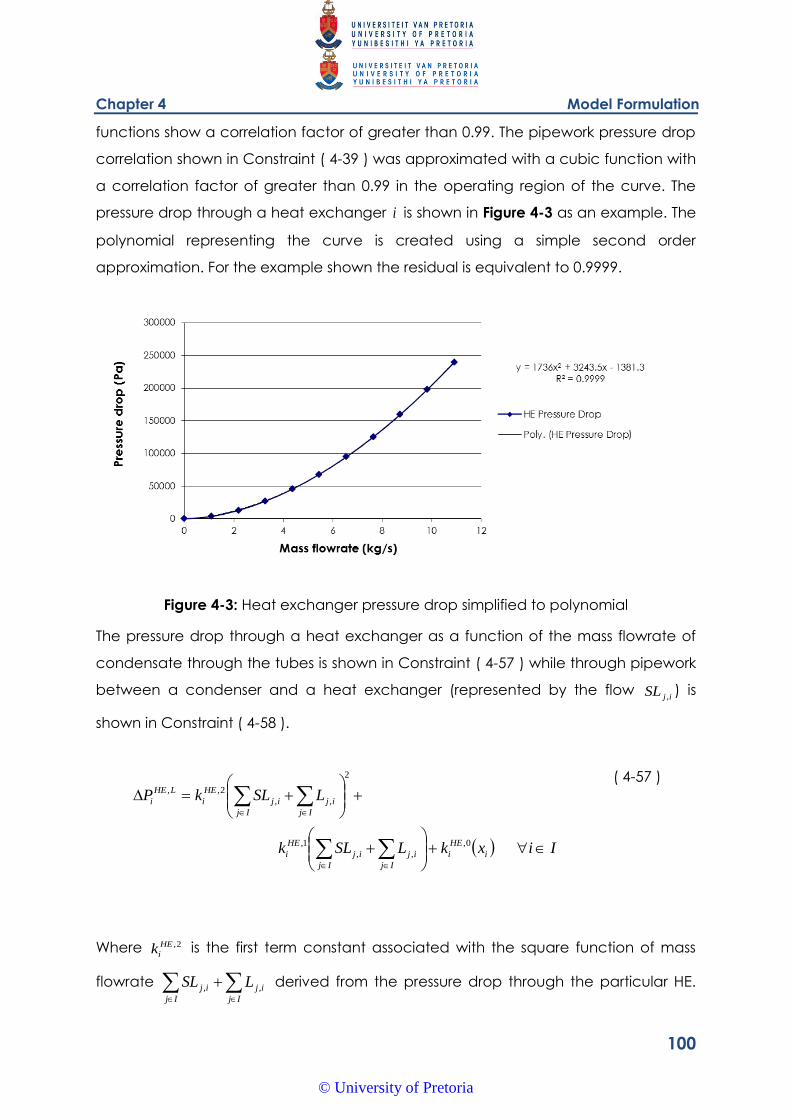
Chapter 4 Model Formulation
100
functions show a correlation factor of greater than 0.99. The pipework pressure drop
correlation shown in Constraint ( 4-39 ) was approximated with a cubic function with
a correlation factor of greater than 0.99 in the operating region of the curve. The
pressure drop through a heat exchanger i is shown in Figure 4-3 as an example. The
polynomial representing the curve is created using a simple second order
approximation. For the example shown the residual is equivalent to 0.9999.
Figure 4-3: Heat exchanger pressure drop simplified to polynomial
The pressure drop through a heat exchanger as a function of the mass flowrate of
condensate through the tubes is shown in Constraint ( 4-57 ) while through pipework
between a condenser and a heat exchanger (represented by the flow ijSL ,) is
shown in Constraint ( 4-58 ).
IixkLSLk
LSLkP
i
HE
i
Ij Ij
ijij
HE
i
Ij Ij
ijij
HE
i
LHE
i
0,
,,
1,
2
,,
2,,
( 4-57 )
Where 2,HE
ik is the first term constant associated with the square function of mass
flowrate
Ij Ij
ijij LSL ,, derived from the pressure drop through the particular HE.
© University of Pretoria
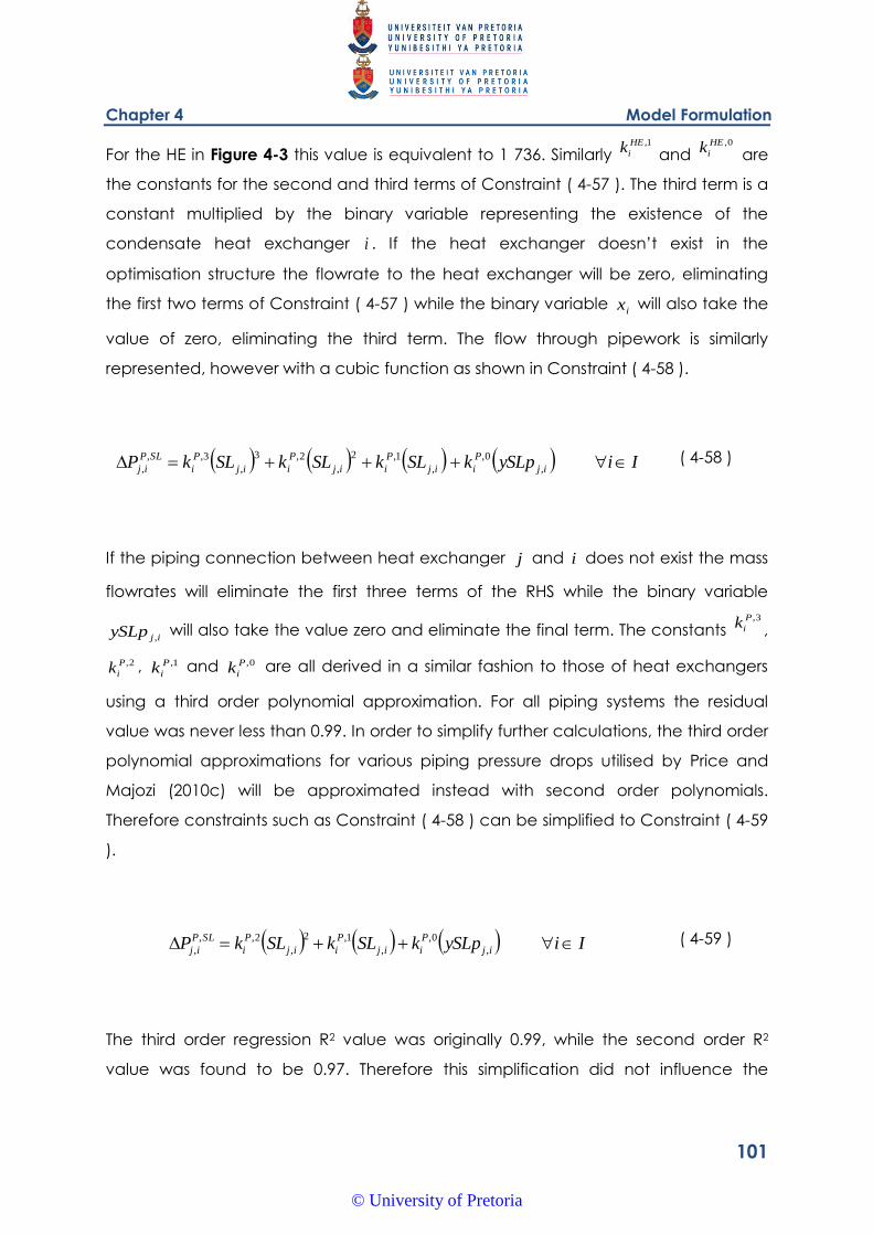
Chapter 4 Model Formulation
101
For the HE in Figure 4-3 this value is equivalent to 1 736. Similarly 1,HE
ik and
0,HE
ik are
the constants for the second and third terms of Constraint ( 4-57 ). The third term is a
constant multiplied by the binary variable representing the existence of the
condensate heat exchanger i . If the heat exchanger doesn’t exist in the
optimisation structure the flowrate to the heat exchanger will be zero, eliminating
the first two terms of Constraint ( 4-57 ) while the binary variable ix will also take the
value of zero, eliminating the third term. The flow through pipework is similarly
represented, however with a cubic function as shown in Constraint ( 4-58 ).
IiySLpkSLkSLkSLkP ij
P
iij
P
iij
P
iij
P
i
SLP
ij ,
0,
,
1,2
,
2,3
,
3,,
, ( 4-58 )
If the piping connection between heat exchanger j and i does not exist the mass
flowrates will eliminate the first three terms of the RHS while the binary variable
ijySLp , will also take the value zero and eliminate the final term. The constants
3,P
ik,
2,P
ik , 1,P
ik and 0,P
ik are all derived in a similar fashion to those of heat exchangers
using a third order polynomial approximation. For all piping systems the residual
value was never less than 0.99. In order to simplify further calculations, the third order
polynomial approximations for various piping pressure drops utilised by Price and
Majozi (2010c) will be approximated instead with second order polynomials.
Therefore constraints such as Constraint ( 4-58 ) can be simplified to Constraint ( 4-59
).
IiySLpkSLkSLkP ij
P
iij
P
iij
P
i
SLP
ij ,
0,
,
1,2
,
2,,
, ( 4-59 )
The third order regression R2 value was originally 0.99, while the second order R2
value was found to be 0.97. Therefore this simplification did not influence the
© University of Pretoria
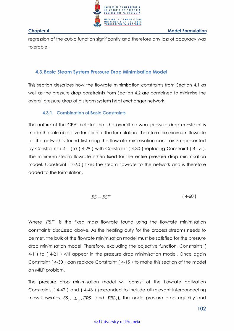
Chapter 4 Model Formulation
102
regression of the cubic function significantly and therefore any loss of accuracy was
tolerable.
4.3. Basic Steam System Pressure Drop Minimisation Model
This section describes how the flowrate minimisation constraints from Section 4.1 as
well as the pressure drop constraints from Section 4.2 are combined to minimise the
overall pressure drop of a steam system heat exchanger network.
4.3.1. Combination of Basic Constraints
The nature of the CPA dictates that the overall network pressure drop constraint is
made the sole objective function of the formulation. Therefore the minimum flowrate
for the network is found first using the flowrate minimisation constraints represented
by Constraints ( 4-1 )to ( 4-29 ) with Constraint ( 4-30 ) replacing Constraint ( 4-15 ).
The minimum steam flowrate isthen fixed for the entire pressure drop minimisation
model. Constraint ( 4-60 ) fixes the steam flowrate to the network and is therefore
added to the formulation.
setFSFS ( 4-60 )
Where setFS is the fixed mass flowrate found using the flowrate minimisation
constraints discussed above. As the heating duty for the process streams needs to
be met, the bulk of the flowrate minimisation model must be satisfied for the pressure
drop minimisation model. Therefore, excluding the objective function, Constraints (
4-1 ) to ( 4-21 ) will appear in the pressure drop minimisation model. Once again
Constraint ( 4-30 ) can replace Constraint ( 4-15 ) to make this section of the model
an MILP problem.
The pressure drop minimisation model will consist of the flowrate activation
Constraints ( 4-42 ) and ( 4-43 ) (expanded to include all relevant interconnecting
mass flowrates iSS ,
ijL ,,
iFRS and iFRL ), the node pressure drop equality and
© University of Pretoria
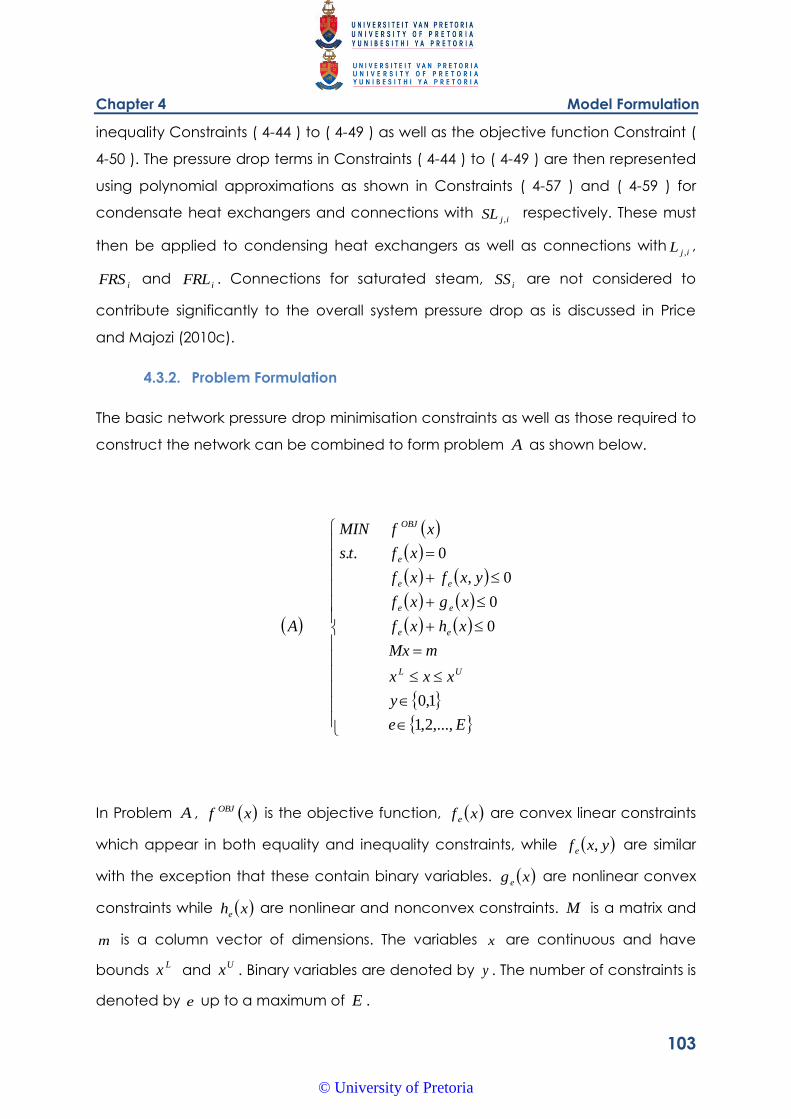
Chapter 4 Model Formulation
103
inequality Constraints ( 4-44 ) to ( 4-49 ) as well as the objective function Constraint (
4-50 ). The pressure drop terms in Constraints ( 4-44 ) to ( 4-49 ) are then represented
using polynomial approximations as shown in Constraints ( 4-57 ) and ( 4-59 ) for
condensate heat exchangers and connections with ijSL , respectively. These must
then be applied to condensing heat exchangers as well as connections withijL ,,
iFRS and iFRL . Connections for saturated steam,
iSS are not considered to
contribute significantly to the overall system pressure drop as is discussed in Price
and Majozi (2010c).
4.3.2. Problem Formulation
The basic network pressure drop minimisation constraints as well as those required to
construct the network can be combined to form problem A as shown below.
Ee
y
xxx
mMx
xhxf
xgxf
yxfxf
xfts
xfMIN
A
UL
ee
ee
ee
e
OBJ
,...,2,1
1,0
0
0
0,
0..
In Problem A , xf OBJ is the objective function, xf e are convex linear constraints
which appear in both equality and inequality constraints, while yxf e , are similar
with the exception that these contain binary variables. xg e are nonlinear convex
constraints while xhe are nonlinear and nonconvex constraints. M is a matrix and
m is a column vector of dimensions. The variables x are continuous and have
bounds Lx and
Ux . Binary variables are denoted by y . The number of constraints is
denoted by e up to a maximum of E .
© University of Pretoria
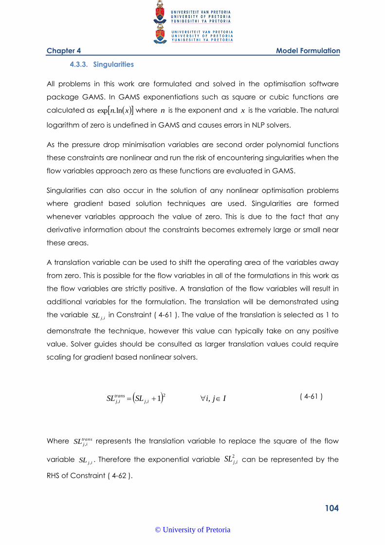
Chapter 4 Model Formulation
104
4.3.3. Singularities
All problems in this work are formulated and solved in the optimisation software
package GAMS. In GAMS exponentiations such as square or cubic functions are
calculated as xn ln.exp where n is the exponent and x is the variable. The natural
logarithm of zero is undefined in GAMS and causes errors in NLP solvers.
As the pressure drop minimisation variables are second order polynomial functions
these constraints are nonlinear and run the risk of encountering singularities when the
flow variables approach zero as these functions are evaluated in GAMS.
Singularities can also occur in the solution of any nonlinear optimisation problems
where gradient based solution techniques are used. Singularities are formed
whenever variables approach the value of zero. This is due to the fact that any
derivative information about the constraints becomes extremely large or small near
these areas.
A translation variable can be used to shift the operating area of the variables away
from zero. This is possible for the flow variables in all of the formulations in this work as
the flow variables are strictly positive. A translation of the flow variables will result in
additional variables for the formulation. The translation will be demonstrated using
the variable ijSL , in Constraint ( 4-61 ). The value of the translation is selected as 1 to
demonstrate the technique, however this value can typically take on any positive
value. Solver guides should be consulted as larger translation values could require
scaling for gradient based nonlinear solvers.
IjiSLSL ij
trans
ij ,12
,, ( 4-61 )
Where trans
ijSL , represents the translation variable to replace the square of the flow
variable ijSL ,. Therefore the exponential variable
2
,ijSL can be represented by the
RHS of Constraint ( 4-62 ).
© University of Pretoria
Chapter 4 Model Formulation
105
IjiSLSLSL ij
trans
ijij ,12 ,,
2
, ( 4-62 )
These translations can be applied to all flow variables. The RHS of Constraint ( 4-62 )
will then replace the term 2
,ijSL in piping connection pressure drop constraints such
as Constraint ( 4-59 ).
4.3.4. Pressure Drop Approximation
By utilising Constraint ( 4-30 ) in place of Constraint ( 4-15 ) in the flowrate
minimisation constraints this portion of the formulation can be linearised. In the entire
pressure drop minimisation problem the only remaining nonlinear constraints are
those representing the pressure drop of the heat exchangers and pipework
connections, represented by Constraints ( 4-57 )and ( 4-59 ) and further expansions
as discussed in Section 4.3.1.
The constraints approximating pressure drop through heat exchangers and pipework
have been simplified to second order polynomial functions. These nonlinear
constraints can be simplified by a number of techniques as discussed below.
Piecewise Linear Approximation
Price and Majozi (2010c) attempted piecewise linear approximations to entirely
represent pressure drop as a function of mass flowrate. This eliminated the nonlinear
aspects of the pressure drop model. A more accurate approximation is to represent
only the nonlinear elements in the pressure drop function using piecewise linear
approximations. As stated above, all pressure drop constraints have been simplified
to second order polynomial functions of mass flowrate. Therefore only the first term
of these approximations will require a piecewise linear approximation to result in the
constraint being linear.
The square terms in the pressure drop approximations are all positive. A square
function 2xxf will be convex in the region where x is positive. Therefore the
approximation of a square flowrate will always be convex in the area of operation.
© University of Pretoria
Chapter 4 Model Formulation
106
Therefore the piecewise approximation of these functions will lead to an
overestimation of the function at all points with the exception of the break points at
which the piecewise linear approximation will equal the function.
Using the steam flowrate variable ijSL , as an example, the above implies that the
piecewise approximation is always greater than or equal to the actual function as
shown in Constraint ( 4-63 ).
RSSIiSLSL iij
pl
ij ,2
,, ( 4-63 )
Where pl
ijSL , is the piecewise linear approximation of 2
,ijSL .
Since the term 2
,ijSL appears with a positive sign in the all second order polynomial
pressure drop approximations, the use of pl
ijSL , as a substitute for 2
,ijSL will lead to an
overestimation of the pressure drop itself. Therefore all solutions using a piecewise
approximation of pressure drop will conservatively overestimate the pressure drop of
the individual element.
Piecewise approximations can be formulated in a number of ways. The
methodology employed in this work will be the same as that of Pörn et al. (2008). This
method will be described below. Figure 4-4 shows an example of the piecewise
approximation of a convex function such as a square function2x . Here binary
variables are used to isolate a section of the linear approximation which can
represent the function in that particular area and allow the function to be modelled
linearly with a small degree of inaccuracy. The break points, represented by 1p to
4p , represent the points where the piecewise approximations are equal to the
function.
© University of Pretoria
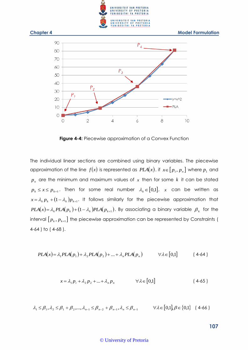
Chapter 4 Model Formulation
107
Figure 4-4: Piecewise approximation of a Convex Function
The individual linear sections are combined using binary variables. The piecewise
approximation of the line xf is represented as xPLA . if nppx ,1 where 1p and
np are the minimum and maximum values of x then for some k it can be stated
1 kk pxp . Then for some real number 1,0k , x can be written as
11 kkkk ppx . It follows similarly for the piecewise approximation that
11 kkkk pPLApPLAxPLA . By associating a binary variable k for the
interval 1, kk pp the piecewise approximation can be represented by Constraints (
4-64 ) to ( 4-68 ).
1,0...2211 nn pPLApPLApPLAxPLA ( 4-64 )
1,0...221 nni pppx ( 4-65 )
1,0,1,0,,...,, 112121211 nnnnn ( 4-66 )
© University of Pretoria
Chapter 4 Model Formulation
108
1,01... 121 n ( 4-67 )
1,01...21 n ( 4-68 )
Constraints ( 4-64 ) to ( 4-68 ) represent a type of ordered set of type 2, or SOS2.
Several MILP solvers can accommodate SOS2 type sets, in which case the piecewise
approximation can be made by excluding Constraint ( 4-67 ) but ensuring that at
most two adjacent k are non-zero.
Relaxation Linearisation
Quesada and Grossmann (1995) used a technique of relaxation and linearisation to
reduce bilinear terms to a single variable. This variable is approximated using the
limits of the two variables constituting the bilinear term. The resulting convex
envelope was first proposed by McCormick (1976). This technique can also be used
to approximate a square term. As the pressure drop constraints are represented as
second order polynomials an opportunity exists to linearise the square term in the
approximation with the over and under estimator technique employed by Quesada
and Grossmann (1995). Using this technique a square term can be aproximated by a
variable as shown in Constraint ( 4-69 ).
IiwSS ii 2
( 4-69 )
In this instance the square of the saturated steam flowrate to a condenser, iSS , is
approximated by iw .
Relaxation linearisation is discussed in more detail in Section 4.5.
© University of Pretoria
Chapter 4 Model Formulation
109
Pressure Drop Approximation in Formulation
By linearising the nonlinear pressure drop terms in the minimum HEN pressure drop
model formulation the constraints xge from Problem A can be approximated by
xg lin
e which has been linearised using either the piecewise linear approximation
technique or a special instance of the relaxation and linearisation technique. This
formulation is presented as problem B .
Ee
y
xxx
mMx
xhxf
xgxf
yxfxf
xfts
xfMIN
B
UL
ee
lin
ee
ee
e
OBJ
,...,2,1
1,0
0
0
0,
0..
4.3.5. Piecewise Approximation with MINLP Solvers
The piecewise linear approximation methodology described above presents an
interesting situation. The exact, nonlinear heat transfer terms require the problem be
formulated as an MINLP. A large number of MINLP solvers utilise an iterative solution
strategy of NLP sub problems along with an MILP master problem. These solvers are
discussed in more detail in Section 3.6. The master problem is an outer
approximation of the constraints and is considered to be a lower bound if it can be
shown that the constraints are convex, or at least pseudo convex within the
operating region of the variables. The different sub problems attempt to converge
on the master problem solution within a certain degree of accuracy. The NLP sub
problems are created by fixing binary variables and solving the subsequent
nonlinear constraints. The solution values of the variables are then taken as points
where linear approximations of the nonlinear constraints are made. This is done in
© University of Pretoria
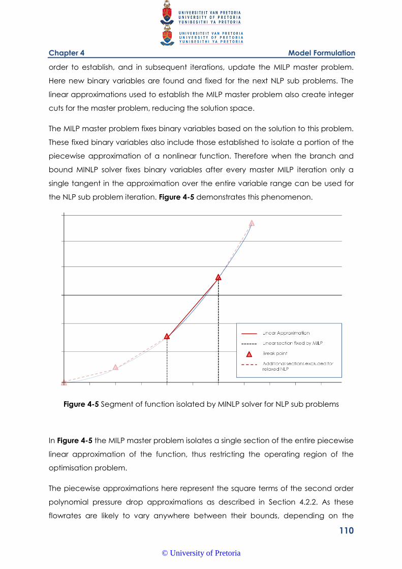
Chapter 4 Model Formulation
110
order to establish, and in subsequent iterations, update the MILP master problem.
Here new binary variables are found and fixed for the next NLP sub problems. The
linear approximations used to establish the MILP master problem also create integer
cuts for the master problem, reducing the solution space.
The MILP master problem fixes binary variables based on the solution to this problem.
These fixed binary variables also include those established to isolate a portion of the
piecewise approximation of a nonlinear function. Therefore when the branch and
bound MINLP solver fixes binary variables after every master MILP iteration only a
single tangent in the approximation over the entire variable range can be used for
the NLP sub problem iteration. Figure 4-5 demonstrates this phenomenon.
Figure 4-5 Segment of function isolated by MINLP solver for NLP sub problems
In Figure 4-5 the MILP master problem isolates a single section of the entire piecewise
linear approximation of the function, thus restricting the operating region of the
optimisation problem.
The piecewise approximations here represent the square terms of the second order
polynomial pressure drop approximations as described in Section 4.2.2. As these
flowrates are likely to vary anywhere between their bounds, depending on the
© University of Pretoria
Chapter 4 Model Formulation
111
network configuration, the restriction to only a small number of sections of the
available solution space for the NLP sub-problems not only greatly reduces the
chances of finding an optimal solution, but from finding a feasible solution.
To overcome these phenomena, fewer linear segments can be used to
approximate nonlinear functions, therefore giving larger solution spaces for NLP sub
problems. The disadvantage of this technique is larger error values between the
piecewise approximation function and the exact function. using more linear
segments may in turn lead to longer solution times as more potentially MILP problems
need to be solved to find a successful combination of variables to satisfy all
constraints. Furthermore, solvers such as DICOPT utilise information from the individual
NLP sub problems. If these sub problems cannot be solved due to an infeasible
solution space provided by the MILP, the NLP sub problem will be infeasible and not
provide any feedback information for the solver.
4.4. Degenerate Solutions
Degenerate solutions are discussed in Section 3.5.1. If degenerate solutions are
allowed for in the formulation the number of feasible HENs that exhibit the minimum
steam flowrate is larger. It is proposed that the additional networks can be
examined to find a better minimum HEN pressure drop than when the optimality
conditions of Savelski and Bagajewicz (2000) are applied to the system.
To utilise degenerate solutions, Constraint ( 4-15 ) is left as a nonlinear constraint. This
constraint exhibits three bilinear terms. These terms will require further processing to
find a feasible, and potentially improved optimal solution.
4.4.1. Temperature and Flow Limits
The outlet temperatures are not necessarily limited between the saturated liquid
temperature and the minimum outlet temperature dictated by the process stream.
The sum of the variations of the outlet temperatures with the minimum outlet
temperatures can be utilised as a limit, just as a minimum mass flowrate limit can be
found for these networks (as shown in Coetzee and Majozi, 2008).
© University of Pretoria
Chapter 4 Model Formulation
112
The sum of deviations of the outlet temperature can be calculated with Constraint (
4-70 ). In the constraint LimoutT , is the sum of the variations while out
iT is the outlet
temperature from heat exchanger i .
Ii
Lout
i
out
i
Limout TTT ,, ( 4-70 )
By calculating the minimum mass flowrate using the technique of Coetzee and
Majozi (2008) the minimum mass flowrate of the system can be calculated. By fixing
the mass flowrate the maximum deviation of the outlet temperatures can be found.
As Constraint ( 4-15 ) this maximisation problem will be formulated as an MINLP.
Constraint ( 4-71 ) can be used to set the minimum mass flowrate for the system
while Constraint ( 4-72 ) can be used to replace Constraint ( 4-29 ) as the objective
function. setFS is the minimum mass flowrate calculated using a technique such as
that of Coetzee and Majozi (2008).
setFSFS ( 4-71 )
LimoutTMinZ , ( 4-72 )
The maximum outlet temperature deviation can be used as a constraint in further
formulations as well as being used as a limit for the individual outlet temperatures.
These limits can be calculated by adding the maximum deviation to the minimum
outlet temperature dictated by the process. This is done by applying Constraint (
4-73 ) to each process stream. If the limit calculated by Constraint ( 4-73 ) is higher
than the saturation temperature, the saturation temperature will become the upper
limit of the outlet temperature.
© University of Pretoria
Chapter 4 Model Formulation
113
IiTTT
T
TTT LimoutLout
i
sat
sat
LimoutLout
iUout
i
,,
,,
, ( 4-73 )
4.5. Relaxation and Linearisation
Quesada and Grossmann (1995) used a technique of relaxation and reformulation
to reduce bilinear terms to a single variable. This variable is approximated using the
limits of the two variables constituting the bilinear term. The resulting convex
envelope was first proposed by McCormick (1976) and later used successfully by
Sherali and Alameddine (1992). This technique will be the first used to overcome the
bilinear terms found in Constraint ( 4-15 ) while attempting to find a minimum
pressure drop from a degenerate flow solution in a heating system. Appendix B
describes this linearisation technique in more detail.
The method of using the relaxation and linearisation technique to solve MINLP
problems with bilinear terms involves linearising the bilinear terms and solving the
resulting model. The solution to this model is then used as a starting point for the
exact model. If the relaxation and linearisation technique results in a linear model
then the solution to this model can be used as a lower bound for a possible globally
optimal solution of the exact model. If the solution to the resulting exact model is
equivalent to the relaxed model then it can be concluded that the solution is
globally optimal.
The pressure drop minimisation formulation described in Section 4.3 contains bilinear
terms in Constraint ( 4-15 ). These terms are the products of the saturated and
subcooled condensate flowrates between heat exchangers i and j with the outlet
temperature of these heat exchangers. Using the liquid flowrate and outlet
temperature from heat exchanger j to heat exchanger i as an example, the
variable ijd , replaces the bilinear term as shown in Constraint ( 4-74 ).
© University of Pretoria
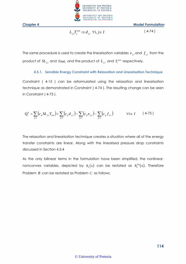
Chapter 4 Model Formulation
114
IjidTL ij
out
jij ,,, ( 4-74 )
The same procedure is used to create the linearisation variables ije , and ijf , from the
product of ijSL , and iTout and the product of ijL , and out
iT respectively.
4.5.1. Sensible Energy Constraint with Relaxation and Linearisation Technique
Constraint ( 4-15 ) can be reformulated using the relaxation and linearisation
technique as demonstrated in Constraint ( 4-74 ). The resulting change can be seen
in Constraint ( 4-75 ).
IifcecdcTSLcQIj Ij
ijpijp
Ij
ijp
ij
satijp
L
i
,,,, ( 4-75 )
The relaxation and linearisation technique creates a situation where all of the energy
transfer constraints are linear. Along with the linearised pressure drop constraints
discussed in Section 4.3.4
As the only bilinear terms in the formulation have been simplified, the nonlinear,
nonconvex variables, depicted by xhe can be restated as xh lin
e. Therefore
Problem B can be restated as Problem C as follows.
© University of Pretoria
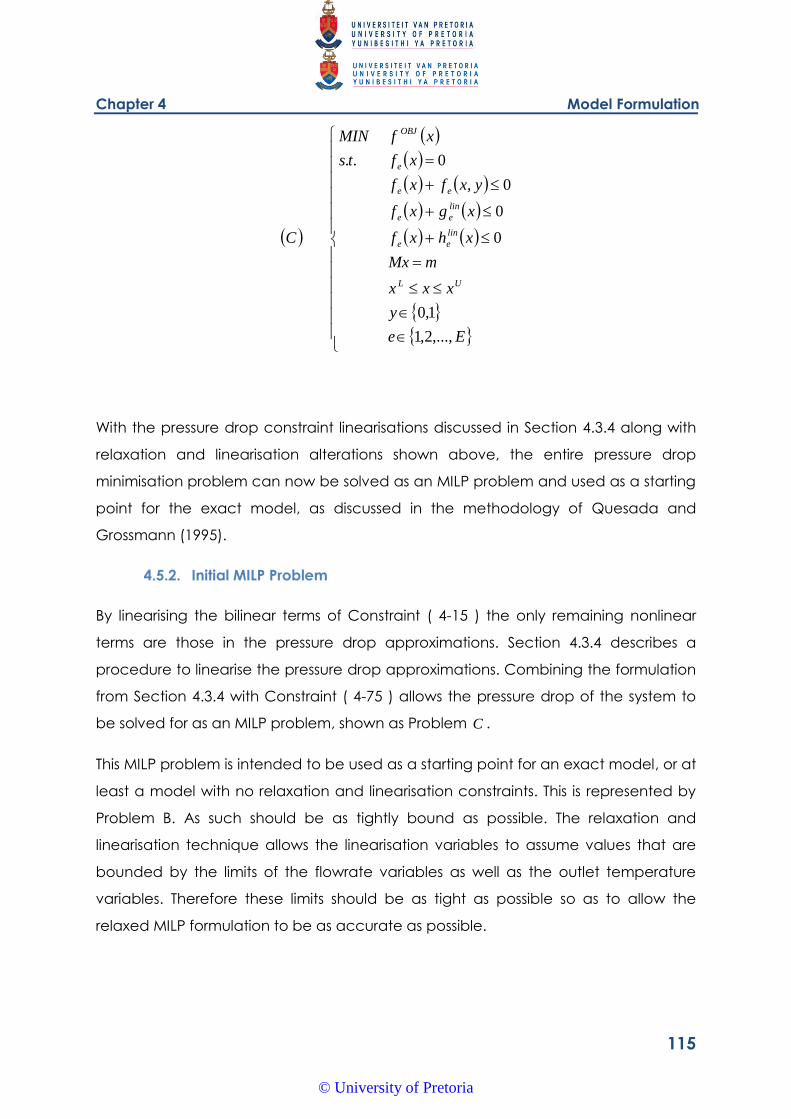
Chapter 4 Model Formulation
115
Ee
y
xxx
mMx
xhxf
xgxf
yxfxf
xfts
xfMIN
C
UL
lin
ee
lin
ee
ee
e
OBJ
,...,2,1
1,0
0
0
0,
0..
With the pressure drop constraint linearisations discussed in Section 4.3.4 along with
relaxation and linearisation alterations shown above, the entire pressure drop
minimisation problem can now be solved as an MILP problem and used as a starting
point for the exact model, as discussed in the methodology of Quesada and
Grossmann (1995).
4.5.2. Initial MILP Problem
By linearising the bilinear terms of Constraint ( 4-15 ) the only remaining nonlinear
terms are those in the pressure drop approximations. Section 4.3.4 describes a
procedure to linearise the pressure drop approximations. Combining the formulation
from Section 4.3.4 with Constraint ( 4-75 ) allows the pressure drop of the system to
be solved for as an MILP problem, shown as Problem C .
This MILP problem is intended to be used as a starting point for an exact model, or at
least a model with no relaxation and linearisation constraints. This is represented by
Problem B. As such should be as tightly bound as possible. The relaxation and
linearisation technique allows the linearisation variables to assume values that are
bounded by the limits of the flowrate variables as well as the outlet temperature
variables. Therefore these limits should be as tight as possible so as to allow the
relaxed MILP formulation to be as accurate as possible.
© University of Pretoria
Chapter 4 Model Formulation
116
Limits for Flow Variables
Limits for the flow variable ijSL , can be found from Constraints ( 4-7 ) and ( 4-19 ).
The maximum amount of saturated condensate available from the outlet of a heat
exchanger is equivalent to the maximum steam flowrate that can flow to that heat
exchanger. Therefore the upper limit of saturated condensate can be found with
Constraint ( 4-76 ).
Ij
QSL
jU
j
( 4-76 )
Similarly the sum of all saturated condensate from heat exchanger j can be
represented by Constraint ( 4-77 ).
IijSLSL U
j
Ii
ij
,, ( 4-77 )
Constraint ( 4-19 ) shows that saturated condensate leaving a heat exchanger can
either be circulated to another heat exchanger or returned to the boiler. Therefore
the limits applying to the flow variable ijSL , also apply to the variable jFRS as
shown in Constraint ( 4-78 ).
IjSLFRS U
jj ( 4-78 )
The subcooled condensate flowrates are more flexible as the sum of all condensate
in the steam system can be fed to heat a single process stream. Therefore the
minimum steam flowrate for the system can be used as a limit for the subcooled
© University of Pretoria
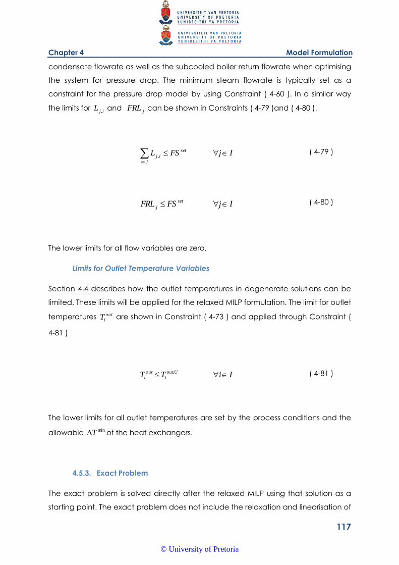
Chapter 4 Model Formulation
117
condensate flowrate as well as the subcooled boiler return flowrate when optimising
the system for pressure drop. The minimum steam flowrate is typically set as a
constraint for the pressure drop model by using Constraint ( 4-60 ). In a similar way
the limits for ijL , and jFRL can be shown in Constraints ( 4-79 )and ( 4-80 ).
IjFSL set
ji
ij
, ( 4-79 )
IjFSFRL set
j ( 4-80 )
The lower limits for all flow variables are zero.
Limits for Outlet Temperature Variables
Section 4.4 describes how the outlet temperatures in degenerate solutions can be
limited. These limits will be applied for the relaxed MILP formulation. The limit for outlet
temperatures out
iT are shown in Constraint ( 4-73 ) and applied through Constraint (
4-81 )
IiTT Uout
i
out
i , ( 4-81 )
The lower limits for all outlet temperatures are set by the process conditions and the
allowable minT of the heat exchangers.
4.5.3. Exact Problem
The exact problem is solved directly after the relaxed MILP using that solution as a
starting point. The exact problem does not include the relaxation and linearisation of
© University of Pretoria
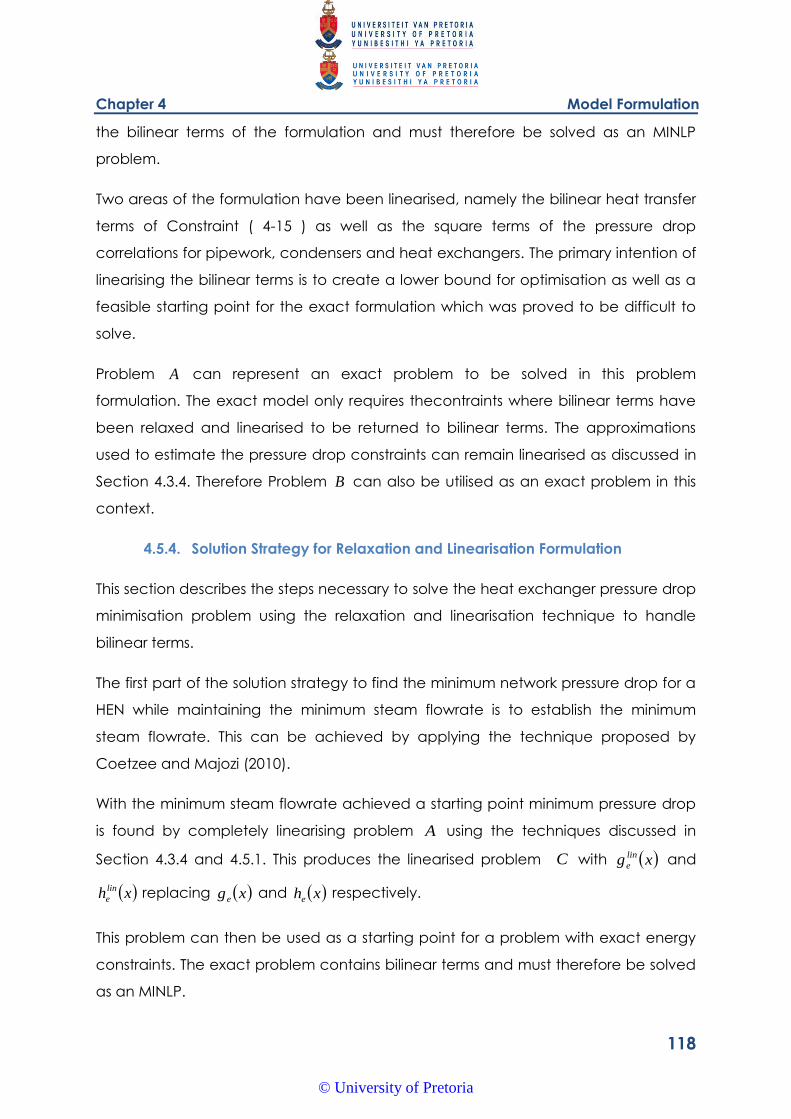
Chapter 4 Model Formulation
118
the bilinear terms of the formulation and must therefore be solved as an MINLP
problem.
Two areas of the formulation have been linearised, namely the bilinear heat transfer
terms of Constraint ( 4-15 ) as well as the square terms of the pressure drop
correlations for pipework, condensers and heat exchangers. The primary intention of
linearising the bilinear terms is to create a lower bound for optimisation as well as a
feasible starting point for the exact formulation which was proved to be difficult to
solve.
Problem A can represent an exact problem to be solved in this problem
formulation. The exact model only requires thecontraints where bilinear terms have
been relaxed and linearised to be returned to bilinear terms. The approximations
used to estimate the pressure drop constraints can remain linearised as discussed in
Section 4.3.4. Therefore Problem B can also be utilised as an exact problem in this
context.
4.5.4. Solution Strategy for Relaxation and Linearisation Formulation
This section describes the steps necessary to solve the heat exchanger pressure drop
minimisation problem using the relaxation and linearisation technique to handle
bilinear terms.
The first part of the solution strategy to find the minimum network pressure drop for a
HEN while maintaining the minimum steam flowrate is to establish the minimum
steam flowrate. This can be achieved by applying the technique proposed by
Coetzee and Majozi (2010).
With the minimum steam flowrate achieved a starting point minimum pressure drop
is found by completely linearising problem A using the techniques discussed in
Section 4.3.4 and 4.5.1. This produces the linearised problem C with xg lin
e and
xh lin
e replacing xge and xhe
respectively.
This problem can then be used as a starting point for a problem with exact energy
constraints. The exact problem contains bilinear terms and must therefore be solved
as an MINLP.
© University of Pretoria
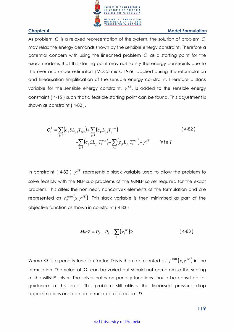
Chapter 4 Model Formulation
119
As problem C is a relaxed representation of the system, the solution of problem C
may relax the energy demands shown by the sensible energy constraint. Therefore a
potential concern with using the linearised problem C as a starting point for the
exact model is that this starting point may not satisfy the energy constraints due to
the over and under estimators (McCormick, 1976) applied during the reformulation
and linearisation simplification of the sensible energy constraint. Therefore a slack
variable for the sensible energy constraint, SE , is added to the sensible energy
constraint ( 4-15 ) such that a feasible starting point can be found. This adjustment is
shown as constraint ( 4-82 ).
IiTLcTSLc
TLcTSLcQ
SE
i
Ij
out
iijp
Ij
out
iijp
Ij
out
jijp
ij
satijp
L
i
,,
,,
( 4-82 )
In constraint ( 4-82 ) SE
i represents a slack variable used to allow the problem to
solve feasibly with the NLP sub problems of the MINLP solver required for the exact
problem. This alters the nonlinear, nonconvex elements of the formulation and are
represented as SErelax
e xh , . This slack variable is then minimised as part of the
objective function as shown in constraint ( 4-83 )
i
SE
iRS PPMinZ ( 4-83 )
Where is a penalty function factor. This is then represented as SEOBJ xf , in the
formulation. The value of can be varied but should not compromise the scaling
of the MINLP solver. The solver notes on penalty functions should be consulted for
guidance in this area. This problem still utilises the linearised pressure drop
approximations and can be formulated as problem D .
© University of Pretoria
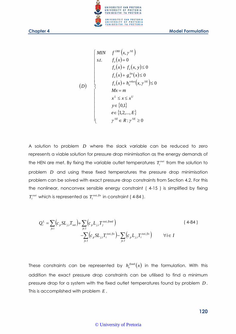
Chapter 4 Model Formulation
120
0:
,...,2,1
1,0
0,
0
0,
0..
,
SESE
UL
SErelax
ee
lin
ee
ee
e
SEOBJ
R
Ee
y
xxx
mMx
xhxf
xgxf
yxfxf
xfts
xfMIN
D
A solution to problem D where the slack variable can be reduced to zero
represents a viable solution for pressure drop minimisation as the energy demands of
the HEN are met. By fixing the variable outlet temperatures out
iT from the solution to
problem D and using these fixed temperatures the pressure drop minimisation
problem can be solved with exact pressure drop constraints from Section 4.2. For this
the nonlinear, nonconvex sensible energy constraint ( 4-15 ) is simplified by fixing
out
iT which is represented as fixout
iT , in constraint ( 4-84 ).
IiTLcTSLc
TLcTSLcQ
Ij
fixout
iijp
Ij
fixout
iijp
Ij
fixedout
jijp
ij
satijp
L
i
,
,
,
,
,
,,
( 4-84 )
These constraints can be represented by xh fixed
e in the formulation. With this
addition the exact pressure drop constraints can be utilised to find a minimum
pressure drop for a system with the fixed outlet temperatures found by problem D .
This is accomplished with problem E .
© University of Pretoria
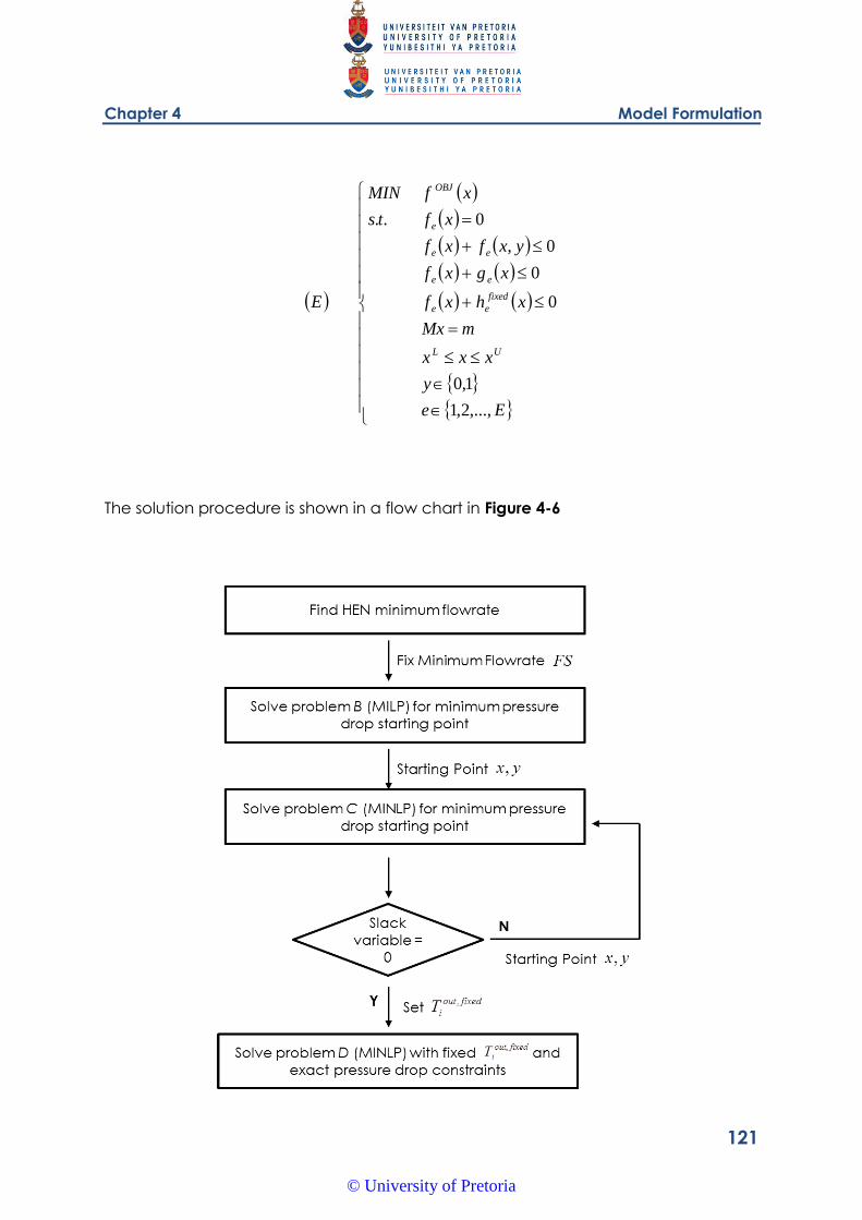
Chapter 4 Model Formulation
121
Ee
y
xxx
mMx
xhxf
xgxf
yxfxf
xfts
xfMIN
E
UL
fixed
ee
ee
ee
e
OBJ
,...,2,1
1,0
0
0
0,
0..
The solution procedure is shown in a flow chart in Figure 4-6
© University of Pretoria
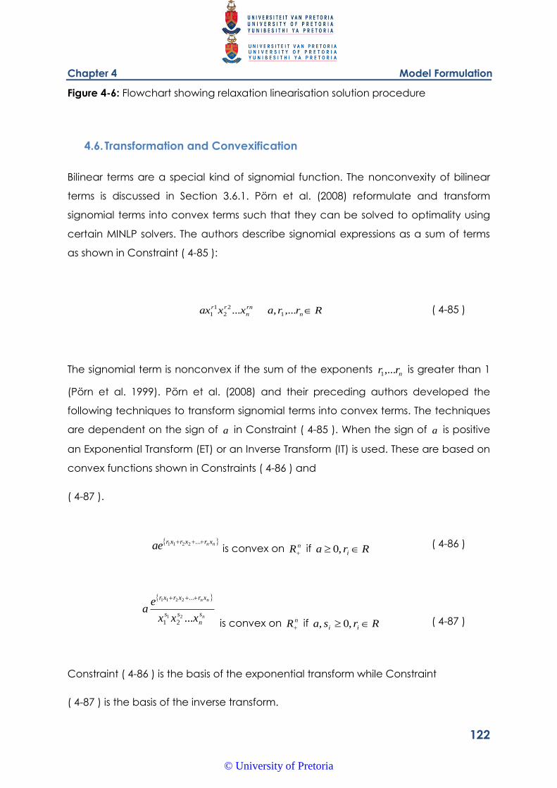
Chapter 4 Model Formulation
122
Figure 4-6: Flowchart showing relaxation linearisation solution procedure
4.6. Transformation and Convexification
Bilinear terms are a special kind of signomial function. The nonconvexity of bilinear
terms is discussed in Section 3.6.1. Pörn et al. (2008) reformulate and transform
signomial terms into convex terms such that they can be solved to optimality using
certain MINLP solvers. The authors describe signomial expressions as a sum of terms
as shown in Constraint ( 4-85 ):
Rrraxxax n
rn
n
rr ,...,... 1
2
2
1
1 ( 4-85 )
The signomial term is nonconvex if the sum of the exponents nrr ,...1 is greater than 1
(Pörn et al. 1999). Pörn et al. (2008) and their preceding authors developed the
following techniques to transform signomial terms into convex terms. The techniques
are dependent on the sign of a in Constraint ( 4-85 ). When the sign of a is positive
an Exponential Transform (ET) or an Inverse Transform (IT) is used. These are based on
convex functions shown in Constraints ( 4-86 ) and
( 4-87 ).
nnxrxrxrae
...2211
is convex on nR if Rra i ,0 ( 4-86 )
n
nn
s
n
ss
xrxrxr
xxx
ea
...21
2211
21
...
is convex on nR if Rrsa ii ,0,
( 4-87 )
Constraint ( 4-86 ) is the basis of the exponential transform while Constraint
( 4-87 ) is the basis of the inverse transform.
© University of Pretoria
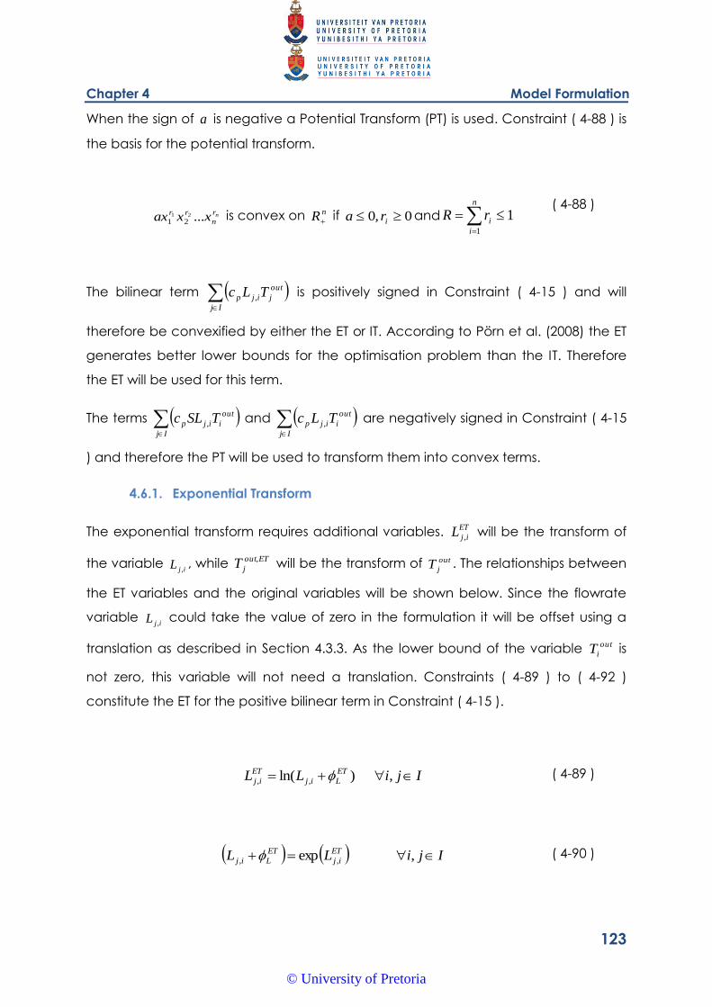
Chapter 4 Model Formulation
123
When the sign of a is negative a Potential Transform (PT) is used. Constraint ( 4-88 ) is
the basis for the potential transform.
nr
n
rrxxax ...21
21 is convex on nR
if 0,0 ira and 11
n
i
irR ( 4-88 )
The bilinear term Ij
out
jijp TLc , is positively signed in Constraint ( 4-15 ) and will
therefore be convexified by either the ET or IT. According to Pörn et al. (2008) the ET
generates better lower bounds for the optimisation problem than the IT. Therefore
the ET will be used for this term.
The terms Ij
out
iijp TSLc , and Ij
out
iijp TLc , are negatively signed in Constraint ( 4-15
) and therefore the PT will be used to transform them into convex terms.
4.6.1. Exponential Transform
The exponential transform requires additional variables. ET
ijL , will be the transform of
the variable ijL ,, while ETout
jT , will be the transform of out
jT . The relationships between
the ET variables and the original variables will be shown below. Since the flowrate
variable ijL , could take the value of zero in the formulation it will be offset using a
translation as described in Section 4.3.3. As the lower bound of the variable out
iT is
not zero, this variable will not need a translation. Constraints ( 4-89 ) to ( 4-92 )
constitute the ET for the positive bilinear term in Constraint ( 4-15 ).
IjiLL ET
Lij
ET
ij ,)ln( ,, ( 4-89 )
IjiLL ET
ij
ET
Lij ,exp ,, ( 4-90 )
© University of Pretoria
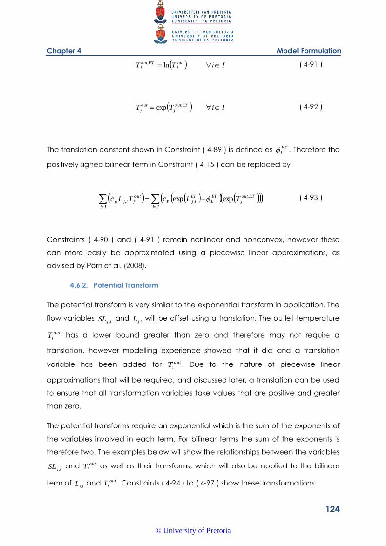
Chapter 4 Model Formulation
124
IiTT out
j
ETout
j ln, ( 4-91 )
IiTT ETout
j
out
j ,exp ( 4-92 )
The translation constant shown in Constraint ( 4-89 ) is defined as ET
L . Therefore the
positively signed bilinear term in Constraint ( 4-15 ) can be replaced by
Ij
ETout
j
ET
L
ET
ijP
Ij
out
jijp TLcTLc ,
,, expexp ( 4-93 )
Constraints ( 4-90 ) and ( 4-91 ) remain nonlinear and nonconvex, however these
can more easily be approximated using a piecewise linear approximations, as
advised by Pörn et al. (2008).
4.6.2. Potential Transform
The potential transform is very similar to the exponential transform in application. The
flow variables ijSL , and
ijL , will be offset using a translation. The outlet temperature
out
iT has a lower bound greater than zero and therefore may not require a
translation, however modelling experience showed that it did and a translation
variable has been added for out
iT . Due to the nature of piecewise linear
approximations that will be required, and discussed later, a translation can be used
to ensure that all transformation variables take values that are positive and greater
than zero.
The potential transforms require an exponential which is the sum of the exponents of
the variables involved in each term. For bilinear terms the sum of the exponents is
therefore two. The examples below will show the relationships between the variables
ijSL , and out
iT as well as their transforms, which will also be applied to the bilinear
term of ijL , and out
iT . Constraints ( 4-94 ) to ( 4-97 ) show these transformations.
© University of Pretoria
Chapter 4 Model Formulation
125
IjiSLSL PT
SLij
PT
ij ,2
,, ( 4-94 )
IjiSLSL PT
ij
PT
SLij ,21
,, ( 4-95 )
IiTT PT
T
out
i
PTout
i out 2, ( 4-96 )
IiTT PTout
i
PT
T
out
i out 21
, ( 4-97 )
Therefore the first negatively signed term in Constraint ( 4-15 )will be replaced by
Constraint ( 4-98 ). The same transformation will then also be needed for the term
Ij
out
iijp TLc , .
IiTSLcTSLcIj
PT
T
PTout
i
PT
SL
PT
ijP
Ij
out
iijp out
21
,21
,,
( 4-98 )
4.6.3. Sensible Energy Constraint with Transformation and Convexification
Section 4.6.1 and Section 4.6.2 allow Constraint ( 4-15 ) to be rewritten as Constraint (
4-99 ).
© University of Pretoria
Chapter 4 Model Formulation
126
Ij
PT
T
PTout
i
PT
L
PT
ijP
Ij
PT
T
PTout
i
PT
SL
PT
ijP
Ij
ETout
j
ET
L
ET
ijP
ij
satijp
L
i
out
out
TLc
TSLc
IiTLcTSLcQ
21
,21
,
21
,21
,
,
,, expexp
( 4-99 )
Constraint ( 4-99 ) needs to be accompanied by the various transformation
constraints for the ET and PT found in Section 4.6.1 and Section 4.6.2 respectively.
4.6.4. Approximation of Nonlinear ET and PT Terms
Pörn et al. (2008) discuss the nonlinear terms created by using the ET and PT. These
terms are approximated by the authors using piecewise linear approximation. A
similar analysis of the orientation of the approximation was done for the pressure
drop approximations in Section 4.3.4 and this will be done for the ET and PT
approximations. As before, all variables that can take a value of zero will be offset
by a translation. The piecewise linearisation of the variable ET
ijL , in the ET is the natural
logarithm of )( ,
ET
LijL . The natural logarithm is a concave function where ijL , is
feasible. Therefore the ET of ijL , can be shown as in Constraint ( 4-100 ).
RLIjiLLL ij
ET
Lij
ET
ij
PLET
ij ,,,
,
, ,,ln ( 4-100 )
Where PLET
ijL ,
, is the piecewise linear approximation of the natural logarithm of the
flow variable ijL , with a translation of ET
L . The exponent of the ET of a variable is
used in Constraint ( 4-99 ) therefore the piecewise linear approximation of the ET will
result in an underestimate of the original variable. This is shown in Figure 4-7. As this
variable represents a positive term in Constraint ( 4-99 ), this transform
underestimates the value of L
iQ in Constraint ( 4-99 ). As the operating range of out
jT
© University of Pretoria
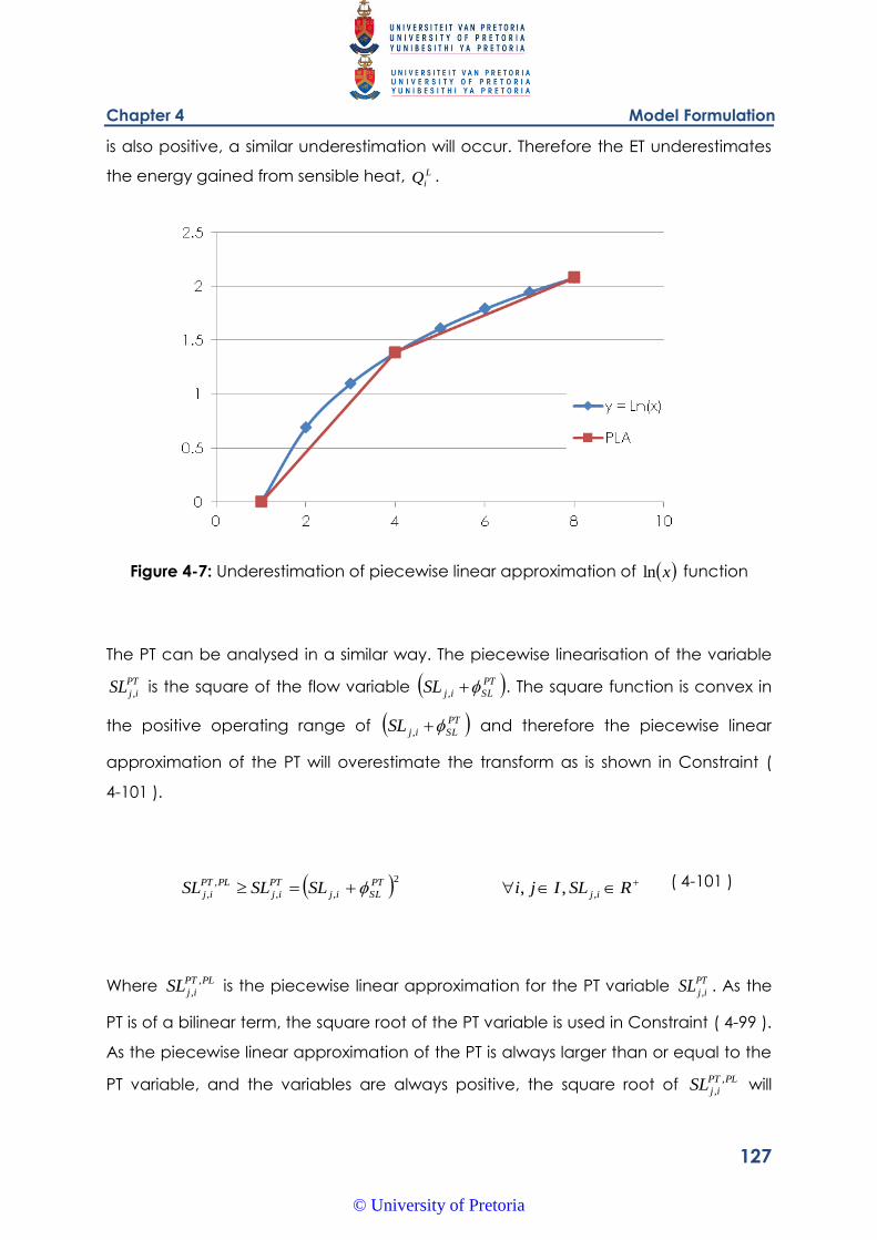
Chapter 4 Model Formulation
127
is also positive, a similar underestimation will occur. Therefore the ET underestimates
the energy gained from sensible heat, L
iQ .
Figure 4-7: Underestimation of piecewise linear approximation of xln function
The PT can be analysed in a similar way. The piecewise linearisation of the variable
PT
ijSL , is the square of the flow variable PT
SLijSL , . The square function is convex in
the positive operating range of PT
SLijSL , and therefore the piecewise linear
approximation of the PT will overestimate the transform as is shown in Constraint (
4-101 ).
RSLIjiSLSLSL ij
PT
SLij
PT
ij
PLPT
ij ,
2
,,
,
, ,, ( 4-101 )
Where PLPT
ijSL ,
, is the piecewise linear approximation for the PT variable PT
ijSL , . As the
PT is of a bilinear term, the square root of the PT variable is used in Constraint ( 4-99 ).
As the piecewise linear approximation of the PT is always larger than or equal to the
PT variable, and the variables are always positive, the square root of PLPT
ijSL ,
, will
© University of Pretoria
Chapter 4 Model Formulation
128
always be larger than or equal to the square root of PT
ijSL , . As the PT variables appear
negatively in Constraint ( 4-99 ) the effect of the piecewise linear approximation on
the PT is to further reduce the value of the energy gained from sensible heat, L
iQ , in
Constraint ( 4-99 ).
Some complexities arise when utilising the piecewise approximations of the ETs and
PTs along with translations. The translations cause additional terms to be required in
the ET and PT approximations of the bilinear terms. For the ET the flow variable ijL ,
and temperature variable out
jT combine as is shown in Constraint ( 4-102 ).
RLIjiTLTL ij
ETout
j
ET
ij
out
jij ,
,
,, ,,exp ( 4-102 )
Therefore using a translation to shift the operation range of the variable ijL , away
from zero, the ET is rewritten as shown in Constraint ( 4-103 ). Constraint ( 4-102 ) can
be rewritten as Constraint ( 4-104 ).
RLIjiLL ij
ET
L
ET
ijij ,,, ,,exp ( 4-103 )
RLIjiTLTL ij
ETout
j
ET
L
ET
ij
out
jij ,
,
,, ,,expexp ( 4-104 )
Therefore the piecewise linear transform appears as Constraint ( 4-105 ).
RLIjiTLTL ij
PLETout
j
ET
L
PLET
ij
out
jij ,
,,,
,, ,,expexp ( 4-105 )
© University of Pretoria
Chapter 4 Model Formulation
129
Considering the nature of the linearisation shown in Figure 4-7 it can be concluded
that the piecewise linear approximation of the ET for the bilinear term out
jij TL ,
always underestimates or is equal to the exact ET as shown in Constraint ( 4-106 ).
RLIjiTL
TL
ij
ETout
j
ET
L
ET
ij
PLETout
j
ET
L
PLET
ij
,
,
,
,,,
,
,,expexp
expexp
( 4-106 )
Similarly, it can be shown that the piecewise linear approximations to the PT
formulations overestimate the exact PT variables as shown in Constraints ( 4-107 )
and ( 4-108 ) respectively.
RSLIjiTSL
TSL
ij
PT
T
PTout
i
PT
SL
PT
ij
PT
T
PLPTout
i
PT
SL
PLPT
ij
out
out
,2
1,2
1
,
21
,,21
,
,
,,
( 4-107 )
RLIjiToutL
ToutL
ij
PT
T
PT
i
PT
L
PT
ij
PT
T
PLPT
i
PT
L
PLPT
ij
out
out
,2
12
1
,
21
,21
,
,
,,
( 4-108 )
Considering that the approximations to the ET underestimate the exact transforms
and those of the PT overestimate the transforms, the energy terms derived by the
bilinear transforms using piecewise linear approximations underestimate the energy
term in Constraint ( 4-99 ), unless all break points from the approximations match
those of the appropriate variables.
This is of large concern as the energy constraints are binding. Therefore it is likely that
infeasibilities will arise in the solving of problems with these formulations unless the
energy term is dealt with specifically. The duty required for each process stream
© University of Pretoria
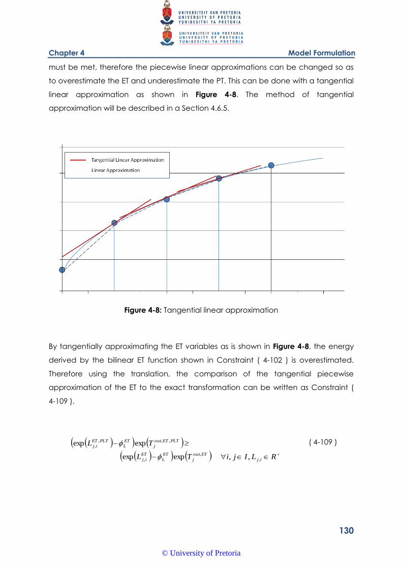
Chapter 4 Model Formulation
130
must be met, therefore the piecewise linear approximations can be changed so as
to overestimate the ET and underestimate the PT. This can be done with a tangential
linear approximation as shown in Figure 4-8. The method of tangential
approximation will be described in a Section 4.6.5.
Figure 4-8: Tangential linear approximation
By tangentially approximating the ET variables as is shown in Figure 4-8, the energy
derived by the bilinear ET function shown in Constraint ( 4-102 ) is overestimated.
Therefore using the translation, the comparison of the tangential piecewise
approximation of the ET to the exact transformation can be written as Constraint (
4-109 ).
RLIjiTL
TL
ij
ETout
j
ET
L
ET
ij
PLTETout
j
ET
L
PLTET
ij
,
,
,
,,,
,
,,expexp
expexp
( 4-109 )
© University of Pretoria
Chapter 4 Model Formulation
131
Where PLTET
ijL ,
, and PLTETout
jT ,, are the tangential piecewise linear approximations of
the ET variables.
Similarly, by using a tangential piecewise approximation, the PT can be
underestimated. Constraints ( 4-110 ) and ( 4-111 ) ensuring that both PTs which
appear negatively in Constraint ( 4-99 ) underestimate the exact PTs.
RSLIjiTSL
TSL
ij
PT
T
PTout
i
PT
SL
PT
ij
PT
T
PLTPTout
i
PT
SL
PLTPT
ij
out
out
,2
1,2
1
,
21
,,21
,
,
,,
( 4-110 )
RLIjiTL
TL
ij
PT
T
PTout
i
PT
L
PT
ij
PT
T
PLTPTout
i
PT
L
PLTPT
ij
out
out
,2
1,2
1
,
21
,,21
,
,
,,
( 4-111 )
Where PLTPT
ijSL ,
, , PLTPTout
iT ,,, PLTPT
ijL ,
, and PLTPTout
iT ,, are the tangential piecewise linear
approximations for the PT variables.
By overestimating the ET variables and underestimating the PT variables, the energy
terms in Constraint ( 4-99 ) will always be overestimated. The sensible energy
constraint can now be rewritten as an inequality shown in Constraint ( 4-112 ).
ij
PT
T
PLTPTout
i
PT
L
PLTPT
ij
ij
PT
T
PLTPTout
i
PT
SL
PLTPT
ij
ij
PLTETout
j
ET
L
PLTET
ij
ij
satijpi
out
out
TL
TSL
IiTLTSLcQL
21
,,21
,
,
21
,,21
,
,
,,,
,, expexp
( 4-112 )
© University of Pretoria
Chapter 4 Model Formulation
132
By using Constraint ( 4-112 ) in the network design constraints the energy gained
from sensible heat by each process stream will be able to be realised, even for the
minimum flowrate which can be found for a heat exchanger network using the
techniques of Coetzee and Majozi (2008).
While Constraint ( 4-112 ) can ensure that the ET and PTs can transform the sensible
heat constraint into a convex term without compromising the other energy balance
constraints, a danger exists that the piecewise linear approximations of the
transforms, which are related to flow and temperature variables, will allow the these
flow and temperature variables to take more favourable values to minimise pressure
drop.
By allowing the sensible energy to take on a larger value due to the piecewise linear
approximations, it is theoretically possible to acquire a lower minimum flowrate to
the system, however this will be a false representation. Therefore when using the ET
and PT in the sensible energy constraint, the minimum flowrate will be set as a
constraint. This flowrate will be found using either the method of Coetzee and Majozi
(2008) or the nonlinear method described in Section 4.1 to give a potential starting
point with variable outlet temperatures.
The piecewise linear approximations also more closely match the exact ET and PT
variables at the break points in the approximations. Therefore, to increase the
accuracy of the optimisation process, an iterative approach is proposed. The break
points will be updated in each step of the iterative process, while a penalty function
will be used to ensure that the flow and temperature variables tend closer to the
break points. The penalty functions will be linked directly to the objective function.
Each iteration will see an update of the break points based on the previous flow and
temperature variable level values.
4.6.5. Tangential Piecewise Linear Approximation
This section will demonstrate the method used to construct the tangential piecewise
linear approximations to the ET and PT variables. The method will be similar to that
employed by Pörn et al. (2008) for conventional piecewise approximation, however
the break points will be used to find tangential intersection points and these will
determine which section of the approximated curve is utilised.
© University of Pretoria
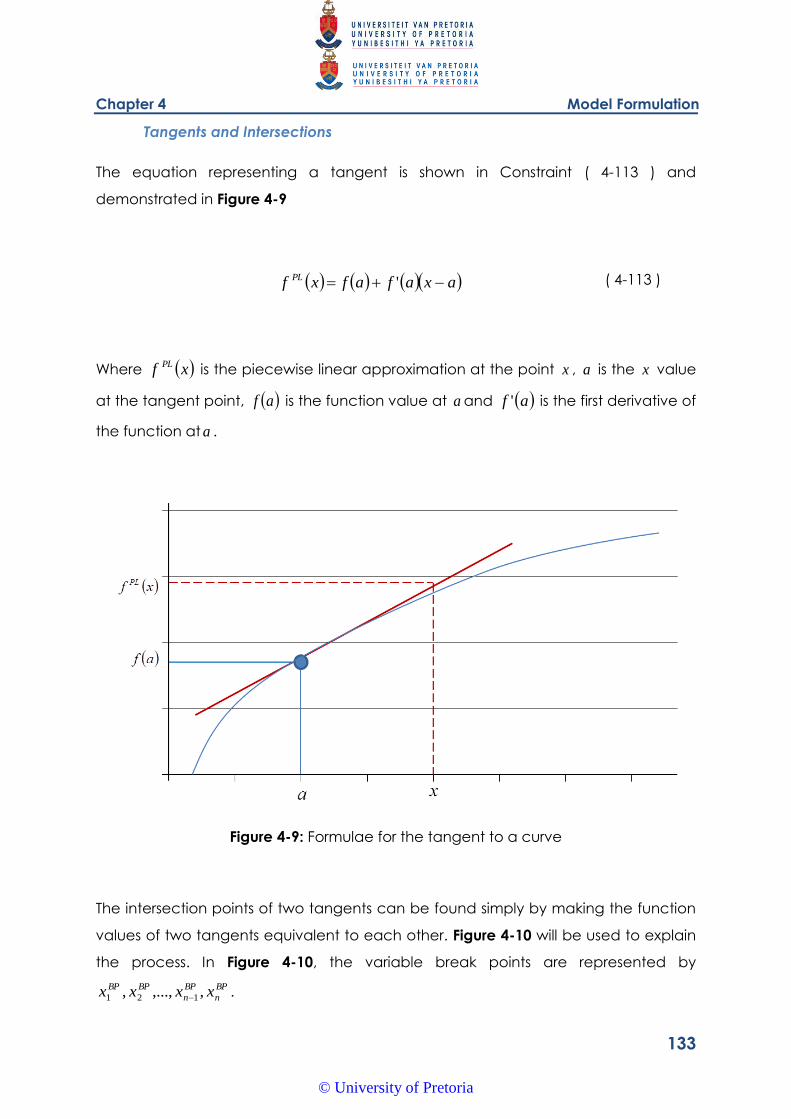
Chapter 4 Model Formulation
133
Tangents and Intersections
The equation representing a tangent is shown in Constraint ( 4-113 ) and
demonstrated in Figure 4-9
axafafxf PL ' ( 4-113 )
Where xf PL is the piecewise linear approximation at the point x , a is the x value
at the tangent point, af is the function value at a and af ' is the first derivative of
the function at a .
Figure 4-9: Formulae for the tangent to a curve
The intersection points of two tangents can be found simply by making the function
values of two tangents equivalent to each other. Figure 4-10 will be used to explain
the process. In Figure 4-10, the variable break points are represented by
BP
n
BP
n
BPBP xxxx ,,...,, 121 .
© University of Pretoria
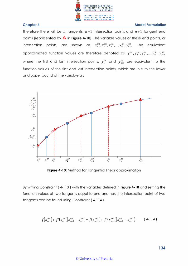
Chapter 4 Model Formulation
134
Therefore there will be n tangents, 1n intersection points and 1n tangent end
points (represented by in Figure 4-10). The variable values of these end points, or
intersection points, are shown as int
1
intint
3
int
2
int
1 ,,...,,, nn xxxxx . The equivalent
approximated function values are therefore denoted as int
1
intint
3
int
2
int
1 ,,...,,, nn yyyyy
where the first and last intersection points, int
1y and int
1ny are equivalent to the
function values of the first and last intersection points, which are in turn the lower
and upper bound of the variable x .
Figure 4-10: Method for Tangential linear approximation
By writing Constraint ( 4-113 ) with the variables defined in Figure 4-10 and setting the
function values of two tangents equal to one another, the intersection point of two
tangents can be found using Constraint ( 4-114 ).
BP
mm
BP
m
BP
m
BP
mm
BP
m
BP
m xxxfxfxxxfxf 1
int
111
int
1 '' ( 4-114 )
© University of Pretoria
Chapter 4 Model Formulation
135
Where m is a value from 1 to n in Figure 4-10. The intersection point int
1mx can then
be solved for as all other values can be calculated from the function and the break
points BP
mx and BP
mx 1 .
Piecewise Approximation Using Multiple Tangents
The same combination of binary variables and fractions used by Pörn et al. (2008)
will be described below, however as opposed to using break points of the piecewise
linear approximations, the intersection points will be used. This formulation is used
widely in literature; however it is not the only formulation and may not necessarily be
the most appropriate.
As described in Figure 4-10 as well as Constraints ( 4-113 ) and ( 4-114 ) the piecewise
linear function will be represented by xf PL and break points by intersection points
int
1
intint
3
int
2
int
1 ,,...,,, nn xxxxx . Therefore if int
1
int
1 , nxxx then there exists a p where
int
1
int
pp xxx . Then for a real number 1,0 , x can be represented as
int
1
int 1 pppp xxx . Therefore the function can be represented as
int
1
int 1 p
PL
pp
PL
p
PL xfxfxf . By utilising a binary variable p to represent
each interval int
1
int , pp xx , the tangential piecewise linear approximation of the ET and
PT variables can be represented by the Constraints ( 4-115 ) to ( 4-119 ).
intint
11
int
22
int
11 ... k
PL
kk
PL
k
PLPLPL xfxfxfxfxf ( 4-115 )
intint
11
int
22
int
11 ... kkkk xxxxx ( 4-116 )
112121211 ,,..., kkkkk ( 4-117 )
© University of Pretoria
Chapter 4 Model Formulation
136
1,01... 121 pk ( 4-118 )
1,01... 121 pkk ( 4-119 )
As was described in Section 4.3.4, if the particular MILP solver used for the
optimisation is compatible with SOS2 variables then the binary component of the
above formulation, Constraints ( 4-116 ) and ( 4-117 ), can be omitted as long as
ensuring that at most two adjacent p are non-zero.
All that remains is to define the function values xf PL for the ET and PT variables.
The ET utilises a natural logarithm function, therefore for a break point or tangential
point BP
mx the function value can be written from Constraint ( 4-113 ) as Constraint (
4-120 ).
a
axaxf PL ln
( 4-120 )
The PT utilises a square function, therefore for a break point or tangential point BP
mx
the function value can be written as Constraint ( 4-121 ).
axaaxf PL 22
( 4-121 )
In the interval formulation represented by Constraints ( 4-115 ) to ( 4-119 ), the
interval function values are calculated using either Constraint ( 4-120 ) or Constraint (
4-121 ) for the ET and PT variables respectively at the interval pointsint
mx .
© University of Pretoria

Chapter 4 Model Formulation
137
These interval points can be calculated before using Constraint ( 4-114 ) and the
pre-defined break points BP
n
BP
n
BPBP xxxx ,,...,, 121 .
4.6.6. Tangential Piecewise Linear Approximation using Branch and Bound
MINLP Algorithms
Section 4.3.5 describes the complexity of using piecewise linear approximation with
branch and bound type MINLP solvers. This section shows this process for tangential
piecewise linear approximation.
When the branch and bound MINLP solver fixes binary variables after every master
MILP iteration, only a small portion of the available break points (as described in
Section 4.6.5) are made available to the NLP solver. This can be seen in Constraint (
4-116 ) where only two of the values will be available to solve the constraint. For
the interval int
nx to int
1nx there exists a single binary variable (either calculated as a
dedicated variable as in Constraint ( 4-117 ) or calculated by the solver in the SOS2
process) which activates the fractions n and 1n . If the values of are limited to
1,0 then if a value of x were to fall outside of the interval of int
nx to int
1nx no
combination of n and 1n would be able to satisfy Constraint ( 4-116 ). This is
further illustrated in Figure 4-11. In the figure the binary variable n activates the
fractions n and 1n allowing these to be solved for the interval between int
nx to
int
1nx , essentially limiting the solution space to this interval.
© University of Pretoria
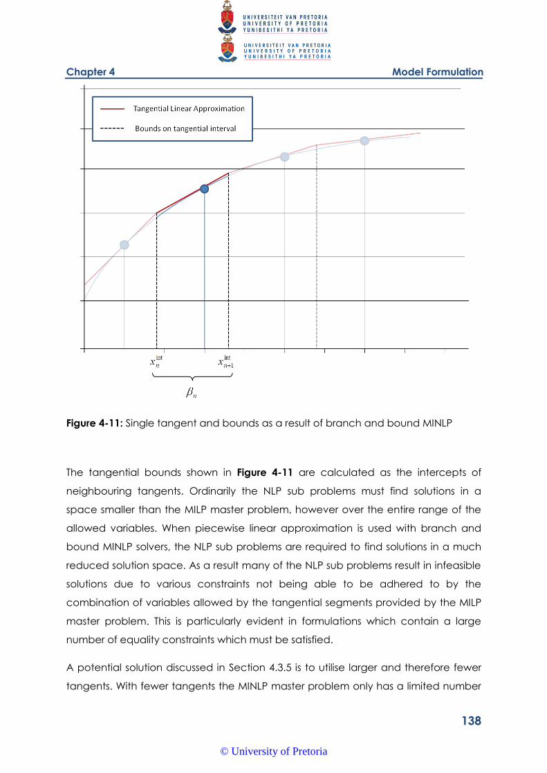
Chapter 4 Model Formulation
138
Figure 4-11: Single tangent and bounds as a result of branch and bound MINLP
The tangential bounds shown in Figure 4-11 are calculated as the intercepts of
neighbouring tangents. Ordinarily the NLP sub problems must find solutions in a
space smaller than the MILP master problem, however over the entire range of the
allowed variables. When piecewise linear approximation is used with branch and
bound MINLP solvers, the NLP sub problems are required to find solutions in a much
reduced solution space. As a result many of the NLP sub problems result in infeasible
solutions due to various constraints not being able to be adhered to by the
combination of variables allowed by the tangential segments provided by the MILP
master problem. This is particularly evident in formulations which contain a large
number of equality constraints which must be satisfied.
A potential solution discussed in Section 4.3.5 is to utilise larger and therefore fewer
tangents. With fewer tangents the MINLP master problem only has a limited number
© University of Pretoria
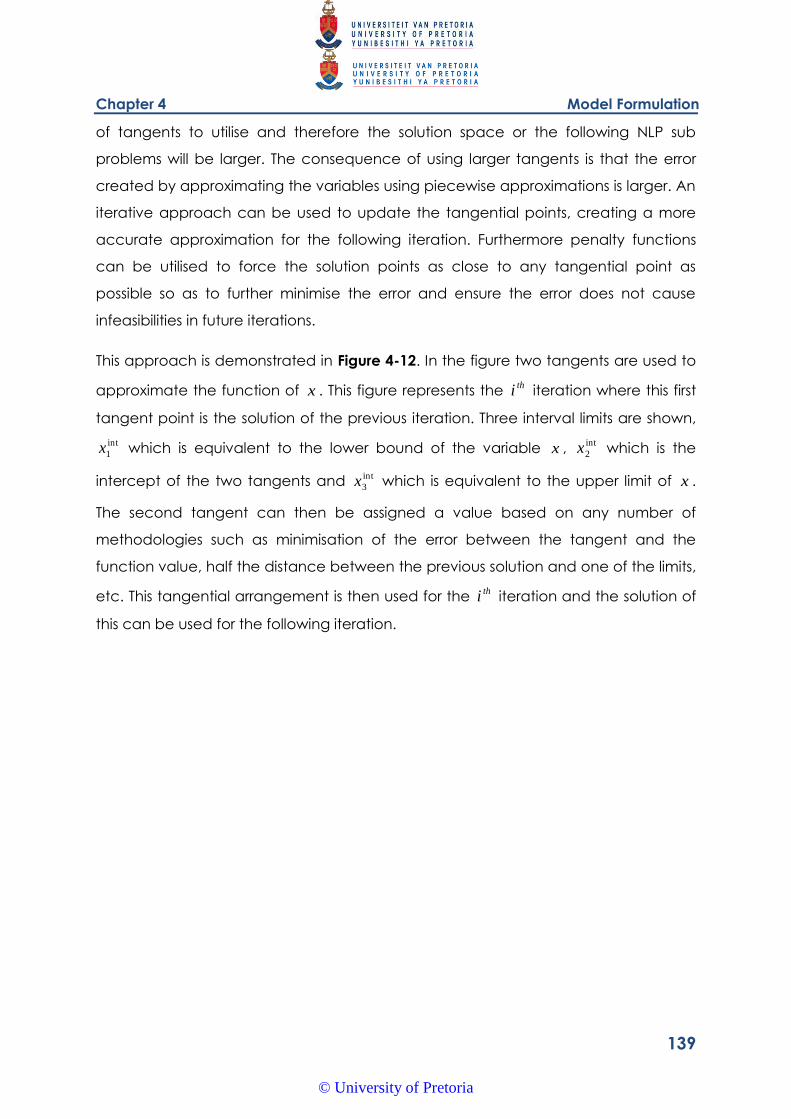
Chapter 4 Model Formulation
139
of tangents to utilise and therefore the solution space or the following NLP sub
problems will be larger. The consequence of using larger tangents is that the error
created by approximating the variables using piecewise approximations is larger. An
iterative approach can be used to update the tangential points, creating a more
accurate approximation for the following iteration. Furthermore penalty functions
can be utilised to force the solution points as close to any tangential point as
possible so as to further minimise the error and ensure the error does not cause
infeasibilities in future iterations.
This approach is demonstrated in Figure 4-12. In the figure two tangents are used to
approximate the function of x . This figure represents the thi iteration where this first
tangent point is the solution of the previous iteration. Three interval limits are shown,
int
1x which is equivalent to the lower bound of the variable x , int
2x which is the
intercept of the two tangents and int
3x which is equivalent to the upper limit of x .
The second tangent can then be assigned a value based on any number of
methodologies such as minimisation of the error between the tangent and the
function value, half the distance between the previous solution and one of the limits,
etc. This tangential arrangement is then used for the thi iteration and the solution of
this can be used for the following iteration.
© University of Pretoria
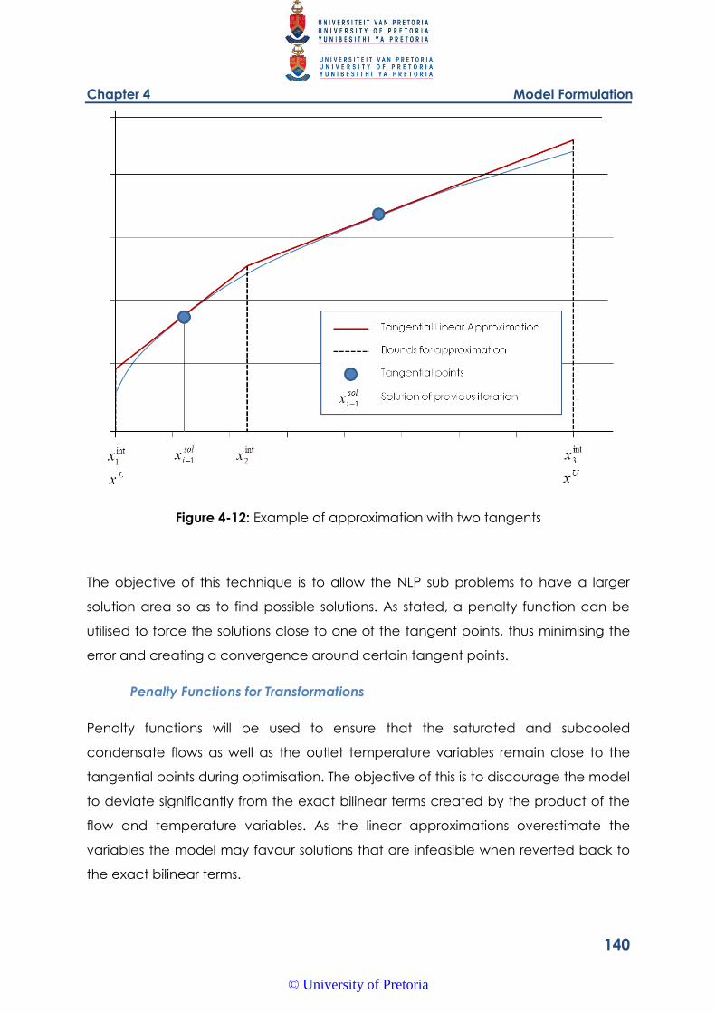
Chapter 4 Model Formulation
140
Figure 4-12: Example of approximation with two tangents
The objective of this technique is to allow the NLP sub problems to have a larger
solution area so as to find possible solutions. As stated, a penalty function can be
utilised to force the solutions close to one of the tangent points, thus minimising the
error and creating a convergence around certain tangent points.
Penalty Functions for Transformations
Penalty functions will be used to ensure that the saturated and subcooled
condensate flows as well as the outlet temperature variables remain close to the
tangential points during optimisation. The objective of this is to discourage the model
to deviate significantly from the exact bilinear terms created by the product of the
flow and temperature variables. As the linear approximations overestimate the
variables the model may favour solutions that are infeasible when reverted back to
the exact bilinear terms.
© University of Pretoria
Chapter 4 Model Formulation
141
The method proposed to implement the penalty functions will be similar to that
discussed in Section 4.5.4, however the variables affected will be the saturated and
subcooled flow variables ijSL , and ijL , as well as the outlet temperature variables
out
iT . As multiple tangent points represent areas where the error between the
piecewise approximation and the function value are zero, solution values near to
any of these points are favourable. If the error was to be calculated between the
variable, say ijSL , , and a single tangent point then the error is simply the absolute
value of the difference between the values. However with multiple tangents the
nearest tangent will have to be selected to calculate the error. This can be
achieved with binary variables, however the same complexity with MILP master
problems isolating binary variables is likely to arise. Therefore it is proposed to instead
apply penalty functions to the additional energy created from the product of the
transformation variables in the sensible energy constraint, shown in Constraint ( 4-112
).
A slack variable can be added to the constraint to represent the additional sensible
energy created from the product of the transformation variables. This constraint is
then reformulated as an equality constraint and shown as Constraint ( 4-122 ).
Iji
TL
TSL
TLTsatSLQL
SE
i
PT
T
PLTPTout
i
PT
L
PLTPT
ij
PT
T
PLTPTout
i
PT
SL
PLTPT
ij
PLTETout
j
ET
L
PLTET
ijiji
out
out
,
expexp
21
,,21
,
,
21
,,21
,
,
,,,
,,
( 4-122 )
In Constraint ( 4-122 ) SE
i is the slack variable used to represent the excess energy
created by the product of the transformation variables. This variable is then assigned
a penalty function and added to the objective function as shown in Constraint (
4-123 ).
© University of Pretoria
Chapter 4 Model Formulation
142
i
SE
iRS PPMinZ ( 4-123 )
Where is some penalty function constant. The values of the penalty function
coefficients will typically be lower than those used for the Relaxation and
Linearisation formulation as the product of two variables is far greater than that of
the individual variables. Also the intention is to typically allow the variables to
deviate from the tangential points slightly if the resulting pressure drop is justified.
Selecting Penalty Coefficients
Several heuristics can be used to aid the selection of the penalty coefficients. The
slack variables added to Constraint ( 4-122 ) allow the energy overestimation as a
result of the linear approximation of the transformation variables to be added to the
objective function and minimised. Essentially these terms in the objective function
will force solution values closer to tangential points, where the linear approximations
and the exact functions are equal. The selection of the coefficients is slightly
complicated by the fact the energy approximation constraints are not directly
related to pressure drop. Therefore a balance of duty feasibility and pressure drop
should be found.
4.6.7. Pressure Drop Constraints in the Transformation and Convexification
Formulation
As in the Relaxation and Linearisation formulation the pressure drop constraints can
be represented exactly as in Problem A or as an approximation as in Problem B .
The approximated pressure drop constraints from Problem B will create the simplest
linear constraints. If the pressure drop constraints are linearised using piecewise
approximation the same complexity as described in Section 4.3.5 will be
encountered. An alternative is to use a single linearisation, which prevents the need
for binary variables. This approach is however not as accurate as piecewise
approximations. Due to the simplicity of the linear approximation for the nonlinear
terms in the pressure drop correlations, these will be used initially to solve the model
© University of Pretoria
Chapter 4 Model Formulation
143
and where necessary these can be made into more accurate piecewise
approximations or exact, nonlinear correlations.
4.6.8. Additional Model Considerations
This section describes further considerations for solving the pressure minimisation
model which include stopping criteria for the model, the initial tangential points and
how these are updated between iterations as well as limits for the transforms.
Stopping Criteria
As linear approximations are made for the energy constraints, it is proposed to test
each solution against the linearised pressure drop model of Price and Majozi
(2010c). Any additional energy gained by the Convexification and Transformation
solution will be assigned to the model of Price and Majozi (2010c) and the resulting
minimum pressure drop solutions will be compared.
It is further proposed that with superior processing power, very precise linear
approximations can be made. This will enable insignificant additional energy to be
made available to the model of Price and Majozi (2010c) and any resulting solutions
could be compared to the reworked results of those authors, as described in Section
4.3.
Initial Tangential Point
The points where tangents are made to the natural logarithms of the ET and the
square functions of the PT will typically be the solution values of the previous
iteration. The first iteration will require starting tangent points.
One option is to use a solution of a simpler problem such as a flowrate minimisation
problem or even utilise the linearised MILP from Section 4.5.2. These solutions can be
used to find the initial tangents for the transformation and convexification solution
strategy.
A further option is to select tangents such that the difference between the tangents
and the curve is minimised. One means to find the minimum difference is to find the
expression for the difference in area below the two curves and minimise this
difference. For single tangents the difference is relatively simple to calculate,
© University of Pretoria
Chapter 4 Model Formulation
144
however for multiple tangents the difference and subsequent minimisation of the
difference becomes more complex.
A further option is to divide the solution space into a number of intervals which is
equivalent to the number of tangents. A tangent is assigned to the middle of each
interval. The end points of the intervals are then based on the intercepts of the
tangents as well as where the tangents cross the boundaries of the solution space.
Updating of Tangential Points
The initial tangential approximations, ma1 will be selected based on any number of
criteria. These include selecting the starting tangents based on solution values of
another model and distributing the remaining tangents according to some method,
minimisation of error between the tangents and the exact function simply to equally
divide the solution space. Thereafter, where feasible, one tangential point will be set
equivalent to the solution variable of the previous solution. Therefore mx
na , is set
equivalent to *
1nx . The other tangents are then distributed throughout the remaining
solution space using any criteria, similar to assigning the initial tangential point.
Limits of Tangents for Potential Transforms
The PT requires square functions of the transformation variables. The linear
approximations for concave square functions have the potential to lead to negative
approximation variables, as demonstrated in Figure 4-13.
© University of Pretoria
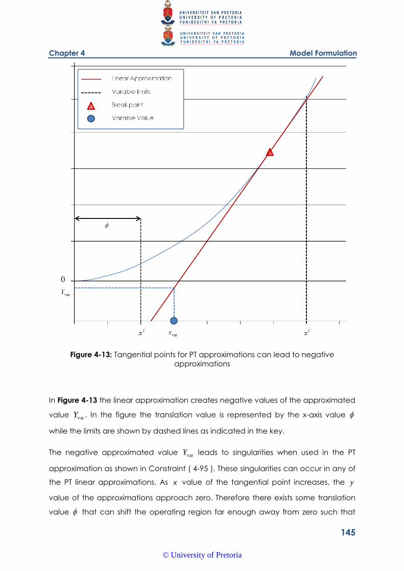
Chapter 4 Model Formulation
145
Figure 4-13: Tangential points for PT approximations can lead to negative
approximations
In Figure 4-13 the linear approximation creates negative values of the approximated
value varY . In the figure the translation value is represented by the x-axis value
while the limits are shown by dashed lines as indicated in the key.
The negative approximated value varY leads to singularities when used in the PT
approximation as shown in Constraint ( 4-95 ). These singularities can occur in any of
the PT linear approximations. As x value of the tangential point increases, the y
value of the approximations approach zero. Therefore there exists some translation
value that can shift the operating region far enough away from zero such that
© University of Pretoria
Chapter 4 Model Formulation
146
any value of x will lead to a corresponding positive y value. This translation value is
dependent on the number of sub divisions for the solution space, divs as well as the
limit values of the variable Lx and
Ux . Constraint ( 4-124 ) shows the appropriate
translation so as to make the tangential points always lead to positive y value
between the limits Lx and
Ux . Constraint ( 4-124 ) can apply to any of the variables
affected by the PT, namely SL , L and outT .
LLU
xdivs
xx
( 4-124 )
4.6.9. Solution strategy for Transformation and Convexification Formulation
A solution strategy will be presented for the linear approximation pressure drop
constraints of Problem B . This strategy will involve an iterative approach where the
tangential points are updated using the most recent solution. Penalty functions are
used to draw the solution variables closer to the tangential points, reducing the
energy over-approximations.
The number of tangents, m
na , can be varied. Section 4.6.6 describes how a larger
number of tangents create smaller individual solution spaces when branch and
bound MINLP solvers are used. More tangents do however create more accurate
solutions. Therefore a balance between accuracy and efficiency should be found.
The number of tangents is represented by m , while the number of iterations is
represented by n .
The basic formulation is presented in Section 4.3.4. The Transformation and
Convexification technique alters Problem B from Section 4.3.4 as by changing xhe
into xxhConv
e~, which are now also a function of transformation variables x~ which
are linked to the exact variables x through the linear approximations denoted by
lxxLT~, . These are shown as Problem F .
© University of Pretoria
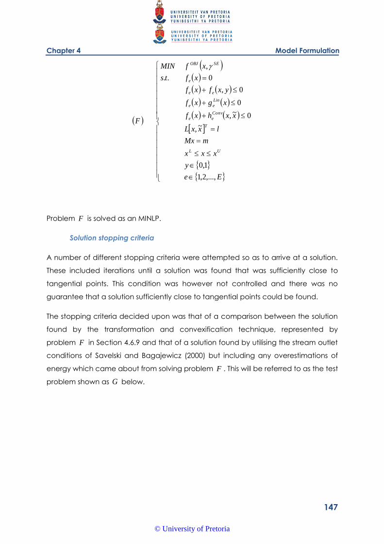
Chapter 4 Model Formulation
147
Ee
y
xxx
mMx
lxxL
xxhxf
xgxf
yxfxf
xfts
xfMIN
F
UL
T
Conv
ee
Lin
ee
ee
e
SEOBJ
,...,2,1
1,0
~,
0~,
0
0,
0..
,
Problem F is solved as an MINLP.
Solution stopping criteria
A number of different stopping criteria were attempted so as to arrive at a solution.
These included iterations until a solution was found that was sufficiently close to
tangential points. This condition was however not controlled and there was no
guarantee that a solution sufficiently close to tangential points could be found.
The stopping criteria decided upon was that of a comparison between the solution
found by the transformation and convexification technique, represented by
problem F in Section 4.6.9 and that of a solution found by utilising the stream outlet
conditions of Savelski and Bagajewicz (2000) but including any overestimations of
energy which came about from solving problem F . This will be referred to as the test
problem shown as G below.
© University of Pretoria
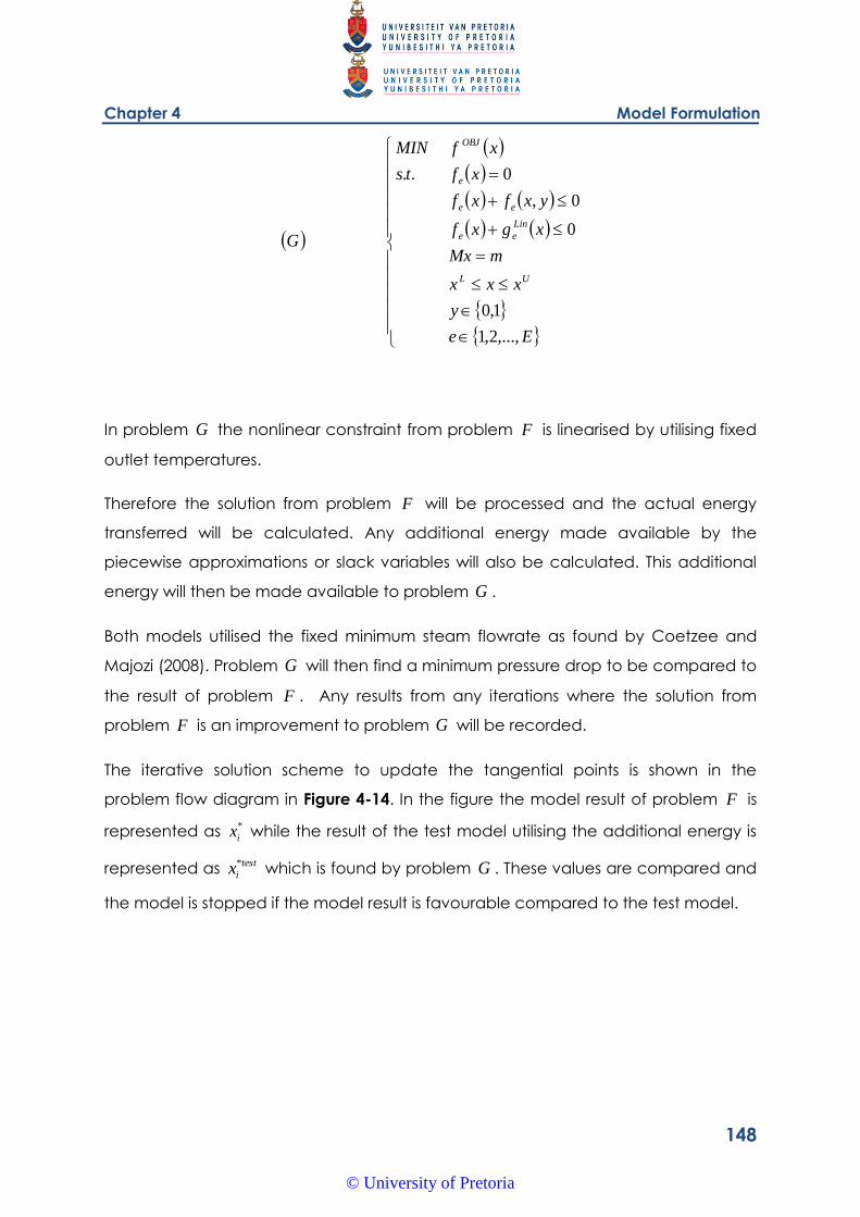
Chapter 4 Model Formulation
148
Ee
y
xxx
mMx
xgxf
yxfxf
xfts
xfMIN
G
UL
Lin
ee
ee
e
OBJ
,...,2,1
1,0
0
0,
0..
In problem G the nonlinear constraint from problem F is linearised by utilising fixed
outlet temperatures.
Therefore the solution from problem F will be processed and the actual energy
transferred will be calculated. Any additional energy made available by the
piecewise approximations or slack variables will also be calculated. This additional
energy will then be made available to problem G .
Both models utilised the fixed minimum steam flowrate as found by Coetzee and
Majozi (2008). Problem G will then find a minimum pressure drop to be compared to
the result of problem F . Any results from any iterations where the solution from
problem F is an improvement to problem G will be recorded.
The iterative solution scheme to update the tangential points is shown in the
problem flow diagram in Figure 4-14. In the figure the model result of problem F is
represented as *
ix while the result of the test model utilising the additional energy is
represented as test
ix* which is found by problem G . These values are compared and
the model is stopped if the model result is favourable compared to the test model.
© University of Pretoria
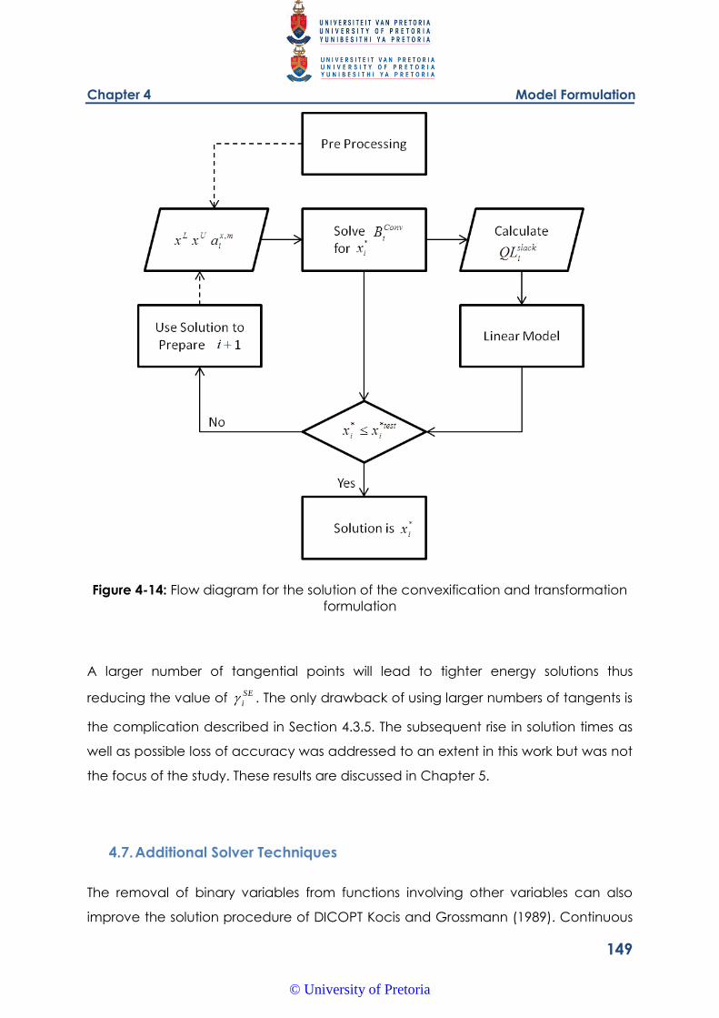
Chapter 4 Model Formulation
149
Figure 4-14: Flow diagram for the solution of the convexification and transformation
formulation
A larger number of tangential points will lead to tighter energy solutions thus
reducing the value of SE
i . The only drawback of using larger numbers of tangents is
the complication described in Section 4.3.5. The subsequent rise in solution times as
well as possible loss of accuracy was addressed to an extent in this work but was not
the focus of the study. These results are discussed in Chapter 5.
4.7. Additional Solver Techniques
The removal of binary variables from functions involving other variables can also
improve the solution procedure of DICOPT Kocis and Grossmann (1989). Continuous
© University of Pretoria
Chapter 4 Model Formulation
150
variables can be used to replace binary variables and then set equivalent to binary
variables in separate constraints. Therefore constraints such as Constraints ( 4-42 )
and ( 4-43 ) will be replaced by Constraints ( 4-125 ) and ( 4-126 ).
0 SLU CySLSL ( 4-125 )
0 SLL CySLSL ( 4-126 )
SLCy is a continuous variable and is made equivalent to the original binary variable
SLy as shown in Constraint ( 4-127 ).
SLSL Cyy ( 4-127 )
4.8. Consideration for Steam System Boiler Efficiency
This section is intended to incorporate the various techniques presented above to
aspects of steam system boiler efficiency.
Boiler efficiency is negatively affected by reducing the steam flowrate of a steam
system. Boiler efficiency is further negatively affected by a reduced condensate
return temperature to the boiler. These phenomena are discussed in Price and
Majozi (2010a). Therefore reducing the steam flowrate to a HEN as suggested by
Coetzee and Majozi (2008) is likely to have negative effects on the boiler efficiency.
A sensitivity analysis of the relationship between return condensate flowrate and
temperature shown in Section 3.4 reveals how if the steam flowrate to a HEN is
reduced the boiler efficiency can be maintained by increasing the condensate
return temperature.
© University of Pretoria
Chapter 4 Model Formulation
151
Price and Majozi (2010a) propose two methods to maintain the boiler efficiency of a
system where the steam flowrate has been reduced. These methods include utilising
the energy lost during let down of the steam to the most appropriate steam pressure
or to include a dedicated heat exchanger in the HEN that will preheat the return
stream to the steam boiler and therefore maintain the boiler efficiency. This heat
exchanger will form part of the normal process optimisation problem.
Of the two methods described, the latter resulted in the more complex MINLP found
in Price and Majozi (2010a). This is due to the variable duty and limiting temperatures
found in this formulation. Therefore it is this MINLP that will be adapted using the
relaxation and linearisation MINLP optimisation technique discussed in Section 4.5 as
well as the transformation and convexification technique discussed in Section 4.6.
4.8.1. Calculation of Boiler Efficiency
The method for the reduction of steam flowrate to a HEN was developed by
Coetzee and Majozi (2008). Section 3.4 showed how reducing the steam flowrate to
a HEN had the effect of reducing the boiler efficiency as a result of the lower
flowrate, as did the lower return temperature to the boiler. The HEN constraints for
single steam pressure level systems shown in Section 4.1 can be used to effectively
find the minimum steam flowrate for a particular HEN. Using this flowrate the new
boiler efficiency for the steam system can be calculated. Several intermediate flow
and temperature variables are required so as to calculate the boiler efficiency.
Figure 4-15 is a reproduction of Figure 3.1 which has been included to show the
origin of certain variables as they relate to the steam system. Additional variables
have been created in amongst the boiler feed water pump and the economiser.
These were not distinguished in Figure 3.1 as they typical form part of a boiler
package.
© University of Pretoria
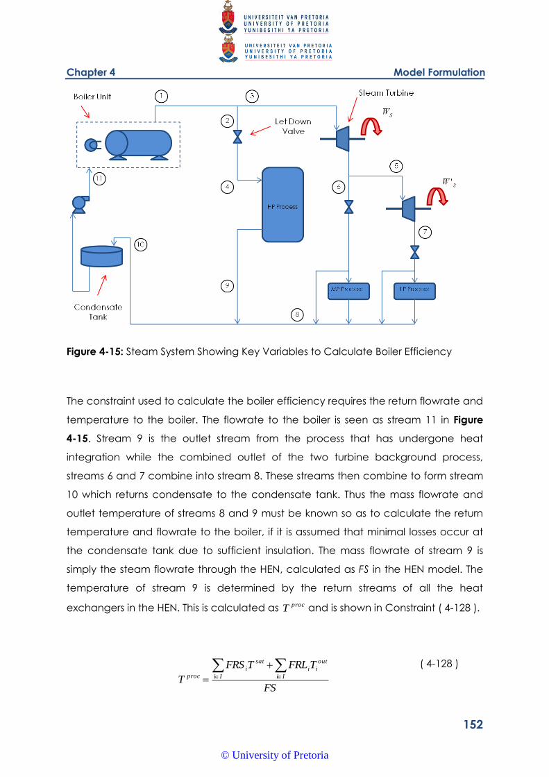
Chapter 4 Model Formulation
152
Figure 4-15: Steam System Showing Key Variables to Calculate Boiler Efficiency
The constraint used to calculate the boiler efficiency requires the return flowrate and
temperature to the boiler. The flowrate to the boiler is seen as stream 11 in Figure
4-15. Stream 9 is the outlet stream from the process that has undergone heat
integration while the combined outlet of the two turbine background process,
streams 6 and 7 combine into stream 8. These streams then combine to form stream
10 which returns condensate to the condensate tank. Thus the mass flowrate and
outlet temperature of streams 8 and 9 must be known so as to calculate the return
temperature and flowrate to the boiler, if it is assumed that minimal losses occur at
the condensate tank due to sufficient insulation. The mass flowrate of stream 9 is
simply the steam flowrate through the HEN, calculated as FS in the HEN model. The
temperature of stream 9 is determined by the return streams of all the heat
exchangers in the HEN. This is calculated as procT and is shown in Constraint ( 4-128 ).
FS
TFRLTFRS
T Ii
out
ii
Ii
sat
iproc
( 4-128 )
© University of Pretoria
Chapter 4 Model Formulation
153
procT represents the return temperature of the process while FS is the mass flowrate.
Stream 9 then combines with stream 8 to form stream 10. If it is assumed that the
mass flowrate to the turbines is constant and that the outlet temperature of the
background processes is also known then the temperature and flowrate of stream 8
will be known and can be assumed constant. These will be referred to as turbT and
turbF in the following constraints respectively. The flowrate of stream 10 is thus simply
the sum of FS and turbF , whereas the temperature is calculated by Constraint (
4-129 ).
turb
turbturbproccoll
FFS
FTFSTT
( 4-129 )
The temperature of Stream 10 is referred to as the collection temperature and is thus
labelled as collT . Stream 10 then enters the condensate tank. Realistically some heat
losses will occur in this area as well as the addition of makeup water to account for
losses from steam traps and blowdown. These factors will be excluded for the
purposes of this investigation but could easily be added as terms to Constraint (
4-129 ). This stream then proceeds to the boiler feed water pump.
Stream 10 passes through the pre heater or economiser, where any additional heat
is represented by Qpreheat. Stream 11 then represents the return stream to the boiler at
flowrate turbFFS and temperature
boilT , calculated in Constraint ( 4-130 ).
turb
P
preheatcollboil
FFSc
QTT
( 4-130 )
© University of Pretoria
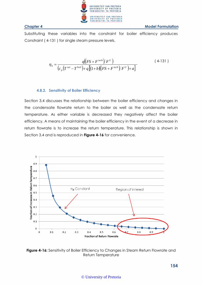
Chapter 4 Model Formulation
154
Substituting these variables into the constraint for boiler efficiency produces
Constraint ( 4-131 ) for single steam pressure levels.
aFFFSbqTTc
FFFSq
Uturbboilsat
p
Uturb
b
1
( 4-131 )
4.8.2. Sensitivity of Boiler Efficiency
Section 3.4 discusses the relationship between the boiler efficiency and changes in
the condensate flowrate return to the boiler as well as the condensate return
temperature. As either variable is decreased they negatively affect the boiler
efficiency. A means of maintaining the boiler efficiency in the event of a decrease in
return flowrate is to increase the return temperature. This relationship is shown in
Section 3.4 and is reproduced in Figure 4-16 for convenience.
Figure 4-16: Sensitivity of Boiler Efficiency to Changes in Steam Return Flowrate and
Return Temperature
© University of Pretoria
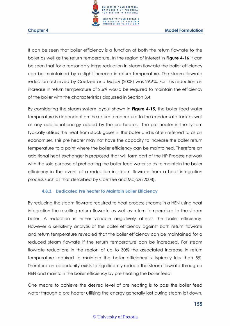
Chapter 4 Model Formulation
155
It can be seen that boiler efficiency is a function of both the return flowrate to the
boiler as well as the return temperature. In the region of interest in Figure 4-16 it can
be seen that for a reasonably large reduction in steam flowrate the boiler efficiency
can be maintained by a slight increase in return temperature. The steam flowrate
reduction achieved by Coetzee and Majozi (2008) was 29.6%. For this reduction an
increase in return temperature of 2.6% would be required to maintain the efficiency
of the boiler with the characteristics discussed in Section 3.4.
By considering the steam system layout shown in Figure 4-15, the boiler feed water
temperature is dependent on the return temperature to the condensate tank as well
as any additional energy added by the pre heater. The pre heater in the system
typically utilises the heat from stack gases in the boiler and is often referred to as an
economiser. This pre heater may not have the capacity to increase the boiler return
temperature to a point where the boiler efficiency can be maintained. Therefore an
additional heat exchanger is proposed that will form part of the HP Process network
with the sole purpose of preheating the boiler feed water so as to maintain the boiler
efficiency in the event of a reduction in steam flowrate from a heat integration
process such as that described by Coetzee and Majozi (2008).
4.8.3. Dedicated Pre heater to Maintain Boiler Efficiency
By reducing the steam flowrate required to heat process streams in a HEN using heat
integration the resulting return flowrate as well as return temperature to the steam
boiler. A reduction in either variable negatively affects the boiler efficiency.
However a sensitivity analysis of the boiler efficiency against both return flowrate
and return temperature revealed that the boiler efficiency can be maintained for a
reduced steam flowrate if the return temperature can be increased. For steam
flowrate reductions in the region of up to 30% the associated increase in return
temperature required to maintain the boiler efficiency is typically less than 5%.
Therefore an opportunity exists to significantly reduce the steam flowrate through a
HEN and maintain the boiler efficiency by pre heating the boiler feed.
One means to achieve the desired level of pre heating is to pass the boiler feed
water through a pre heater utilising the energy generally lost during steam let down.
© University of Pretoria
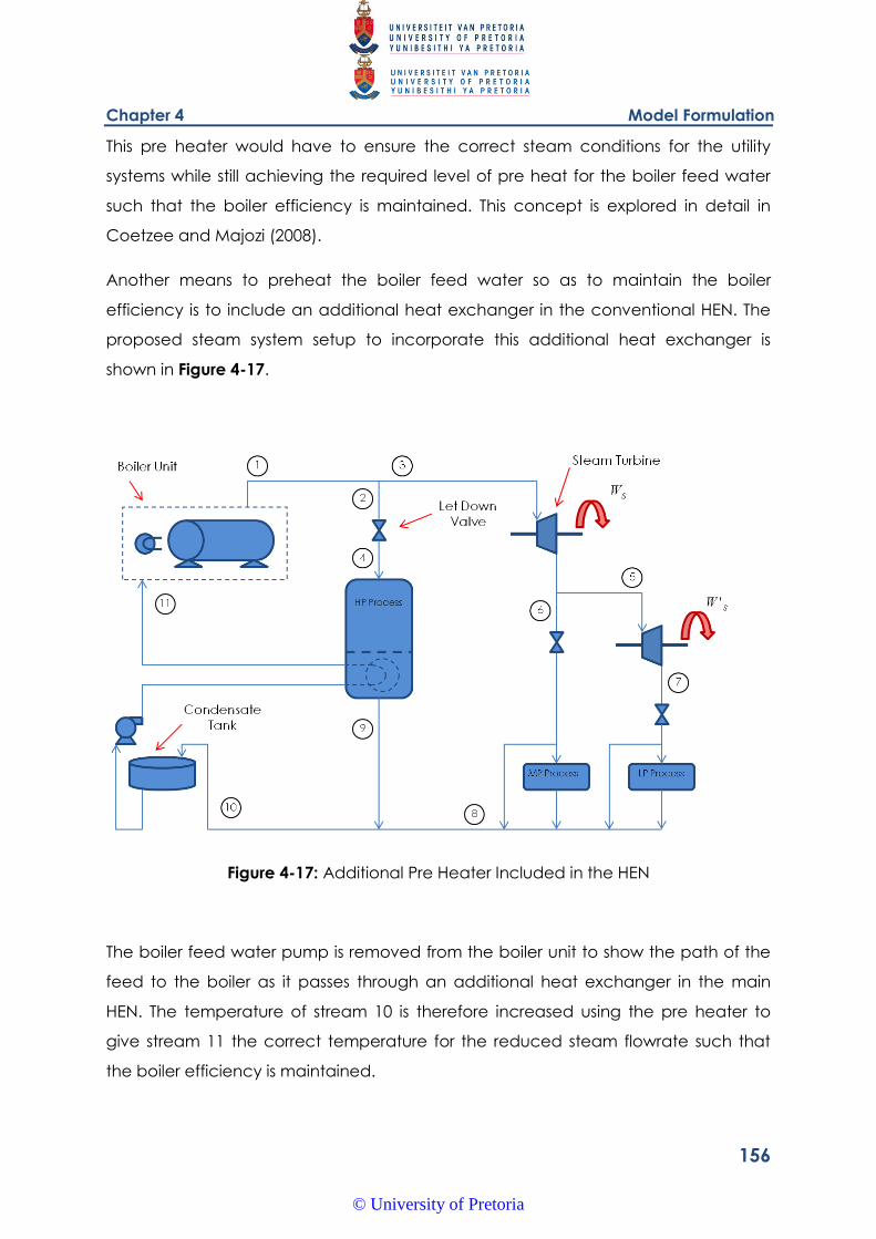
Chapter 4 Model Formulation
156
This pre heater would have to ensure the correct steam conditions for the utility
systems while still achieving the required level of pre heat for the boiler feed water
such that the boiler efficiency is maintained. This concept is explored in detail in
Coetzee and Majozi (2008).
Another means to preheat the boiler feed water so as to maintain the boiler
efficiency is to include an additional heat exchanger in the conventional HEN. The
proposed steam system setup to incorporate this additional heat exchanger is
shown in Figure 4-17.
Figure 4-17: Additional Pre Heater Included in the HEN
The boiler feed water pump is removed from the boiler unit to show the path of the
feed to the boiler as it passes through an additional heat exchanger in the main
HEN. The temperature of stream 10 is therefore increased using the pre heater to
give stream 11 the correct temperature for the reduced steam flowrate such that
the boiler efficiency is maintained.
© University of Pretoria
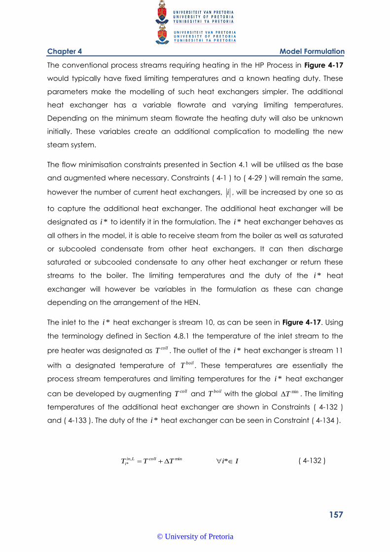
Chapter 4 Model Formulation
157
The conventional process streams requiring heating in the HP Process in Figure 4-17
would typically have fixed limiting temperatures and a known heating duty. These
parameters make the modelling of such heat exchangers simpler. The additional
heat exchanger has a variable flowrate and varying limiting temperatures.
Depending on the minimum steam flowrate the heating duty will also be unknown
initially. These variables create an additional complication to modelling the new
steam system.
The flow minimisation constraints presented in Section 4.1 will be utilised as the base
and augmented where necessary. Constraints ( 4-1 ) to ( 4-29 ) will remain the same,
however the number of current heat exchangers, i , will be increased by one so as
to capture the additional heat exchanger. The additional heat exchanger will be
designated as *i to identify it in the formulation. The *i heat exchanger behaves as
all others in the model, it is able to receive steam from the boiler as well as saturated
or subcooled condensate from other heat exchangers. It can then discharge
saturated or subcooled condensate to any other heat exchanger or return these
streams to the boiler. The limiting temperatures and the duty of the *i heat
exchanger will however be variables in the formulation as these can change
depending on the arrangement of the HEN.
The inlet to the *i heat exchanger is stream 10, as can be seen in Figure 4-17. Using
the terminology defined in Section 4.8.1 the temperature of the inlet stream to the
pre heater was designated as collT . The outlet of the *i heat exchanger is stream 11
with a designated temperature of boilT . These temperatures are essentially the
process stream temperatures and limiting temperatures for the *i heat exchanger
can be developed by augmenting collT and
boilT with the global minT . The limiting
temperatures of the additional heat exchanger are shown in Constraints ( 4-132 )
and ( 4-133 ). The duty of the *i heat exchanger can be seen in Constraint ( 4-134 ).
IiTTT collLin
i *min,
* ( 4-132 )
© University of Pretoria
Chapter 4 Model Formulation
158
IiTTT boilLout
i *min,
* ( 4-133 )
IiTTFc
TLcTSLcSSQ
boilout
iP
Ij
out
jijP
Ij
sat
ijPii
*min
*
*,*,**
( 4-134 )
The temperature of the stream returning to the boiler, boilT , was calculated in
Constraint ( 4-130 ) by adding energy gained by the pre heater to the stream
leaving the condensate tank, collT . This is now shown by the energy added to stream
10 as being the duty of the *i heat exchanger. This is represented in Constraint (
4-135 ).
turb
P
icollboil
FFSc
QTT
*
( 4-135 )
The basic boiler efficiency constraints are shown in Section 4.8.1. Therefore
Constraints ( 4-128 ) to ( 4-131 ) with Constraint ( 4-135 ) replacing Constraint ( 4-130 )
will complete the formulation. It remains to specify an objective function for this
formulation. The objective is, as in the work of Coetzee and Majozi (2008) to minimise
the steam flowrate to the HEN. The boiler efficiency is therefore set as a parameter in
the formulation and the objective function is to reduce the steam flowrate as far as
possible.
Without considering the boiler efficiency the minimum steam flowrate for the HEN
can be found using the technique of Coetzee and Majozi (2008) shown in Section
4.1. The result of this process is a minimum steam flowrate FS . This solution can be
used as a starting point for the next objective of maintaining the boiler efficiency. As
additional steam will be required to pre heat the boiler return, an additional slack
variable is added to the minimum steam flowrate FS . The objective will therefore be
© University of Pretoria
Chapter 4 Model Formulation
159
to minimise this slack variable. The addition of the slack variable will be shown in the
appropriate boiler efficiency constraints below as well as the new objective
function. Constraints ( 4-136 ) to ( 4-139 ) will allow the boiler efficiency to be
accounted for. B in Constraint ( 4-139 ) will be set as a constant equivalent to that
of the steam system before heat integration. Constraint ( 4-140 ) then represents the
objective function. The slack variable for boiler efficiency problems is represented by
BE .
BE
Ii
out
ii
Ii
sat
i
proc
FS
TFRLTFRS
T
( 4-136 )
turbBE
turbturbBEproccoll
FFS
FTFSTT
( 4-137 )
turbBE
P
preheatcollboil
FFSc
QTT
( 4-138 )
aFFFSbqTTc
FFFSq
UturbBEboilsat
p
UturbBE
b
1
( 4-139 )
BEMinZ ( 4-140 )
Therefore this formulation includes the HEN steam flowrate minimisation constraints
found in Section 4.1, namely Constraints ( 4-1 ) to ( 4-29 ), with the objective function
replaced by Constraint ( 4-140 ). Then the boiler efficiency constraints discussed
© University of Pretoria
Chapter 4 Model Formulation
160
above, Constraints ( 4-136 ) to ( 4-139 ) as well as the considerations for the limiting
temperatures and the duty of the *i heat exchanger, Constraints ( 4-132 ) to ( 4-134
) make up the formulation to reduce steam flowrate to a HEN while maintaining the
boiler efficiency with a dedicated boiler feed water pre heater.
This formulation contains a number of non linear terms making the problem an
MINLP. The variable product terms are bilinear, making the problem nonconvex.
Price and Majozi (2010a) catered for the bilinear terms in the sensible energy
constraint by setting the outlet temperatures to their limits using the principle applied
by Savelski and Bagajewicz (2000). The bilinear boiler efficiency terms were handled
using the technique of Quesada and Grossmann (1994), described in Section 4.5. In
this work the limiting temperature constraint of Savelski and Bagajewicz (2000) will be
relaxed. All of the bilinear terms will be handled using the relaxation and linearisation
technique discussed in Section 4.5 as well as the transformation and convexification
technique discussed in Section 4.6.
4.8.4. Solution Strategy
The same bilinear terms exist in Constraint ( 4-15 ) as were found in the pressure drop
minimisation problem. These terms will be dealt with in the same way as discussed in
Section 4.5 and Section 4.6. Additional bilinear terms are found in the boiler
efficiency constraints. These are listed below:
out
iT and iFRL ;
procT and FS ;
procT and BE ;
collT and FS ;
collT and BE ;
boilT and FS ; and
boilT and
BE .
A number of bilinear terms are brought about by the variable nature of the duty for
the *i heat exchanger. Constraints ( 4-22 ) and ( 4-23 ) are typically linear, however
with a variable duty two bilinear terms are formed. These are listed below:
© University of Pretoria
Chapter 4 Model Formulation
161
*iQ and *iy ; and
*iQ and *ix .
As *iy and *ix are binary variables these bilinear terms can be dealt with by the
Glover Transformation (Glover, 1975). This is discussed further in Appendix B.
Relaxation and Linearisation
The relaxation and linearisation technique was applied to the variables in the boiler
efficiency constraints by Price and Majozi (2010a). The formulations will be used as
such. The allowance for degenerate solutions will be catered for in the same way as
was discussed in Section 4.5. Key focus elements of the solution strategy from
Sections 4.5.2, 4.5.3 and 4.5.4 such as variable limits will also be applied, as well as
those additional solver techniques as discussed in Section 4.7.
Transformation and Convexification
The various bilinear terms will have the ET or PT applied to them depending on their
sign in the constraint they appear in. As they do not all occur in the same
constraints, the signs of the various terms with respect to each other will be utilised to
determine whether the ET or PT is applied to the various bilinear terms.
The transformations are designated and shown in Table 4-1.
© University of Pretoria
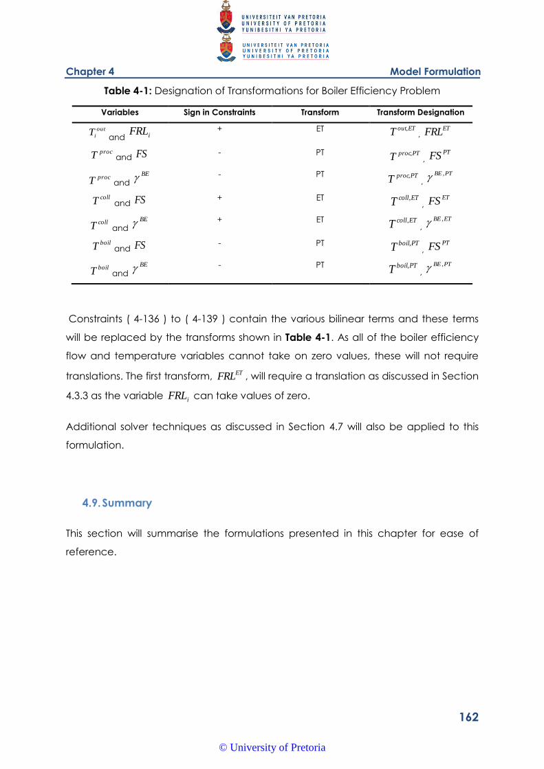
Chapter 4 Model Formulation
162
Table 4-1: Designation of Transformations for Boiler Efficiency Problem
Variables Sign in Constraints Transform Transform Designation
out
iT and iFRL
+ ET EToutT ,
, ETFRL
procT and FS - PT PTprocT ,
, PTFS
procT and BE
- PT PTprocT ,
, PTBE ,
collT and FS + ET ETcollT ,
, ETFS
collT and BE
+ ET ETcollT ,
, ETBE ,
boilT and FS - PT PTboilT ,
, PTFS
boilT and BE
- PT PTboilT ,
, PTBE ,
Constraints ( 4-136 ) to ( 4-139 ) contain the various bilinear terms and these terms
will be replaced by the transforms shown in Table 4-1. As all of the boiler efficiency
flow and temperature variables cannot take on zero values, these will not require
translations. The first transform, ETFRL , will require a translation as discussed in Section
4.3.3 as the variable iFRL can take values of zero.
Additional solver techniques as discussed in Section 4.7 will also be applied to this
formulation.
4.9. Summary
This section will summarise the formulations presented in this chapter for ease of
reference.
© University of Pretoria
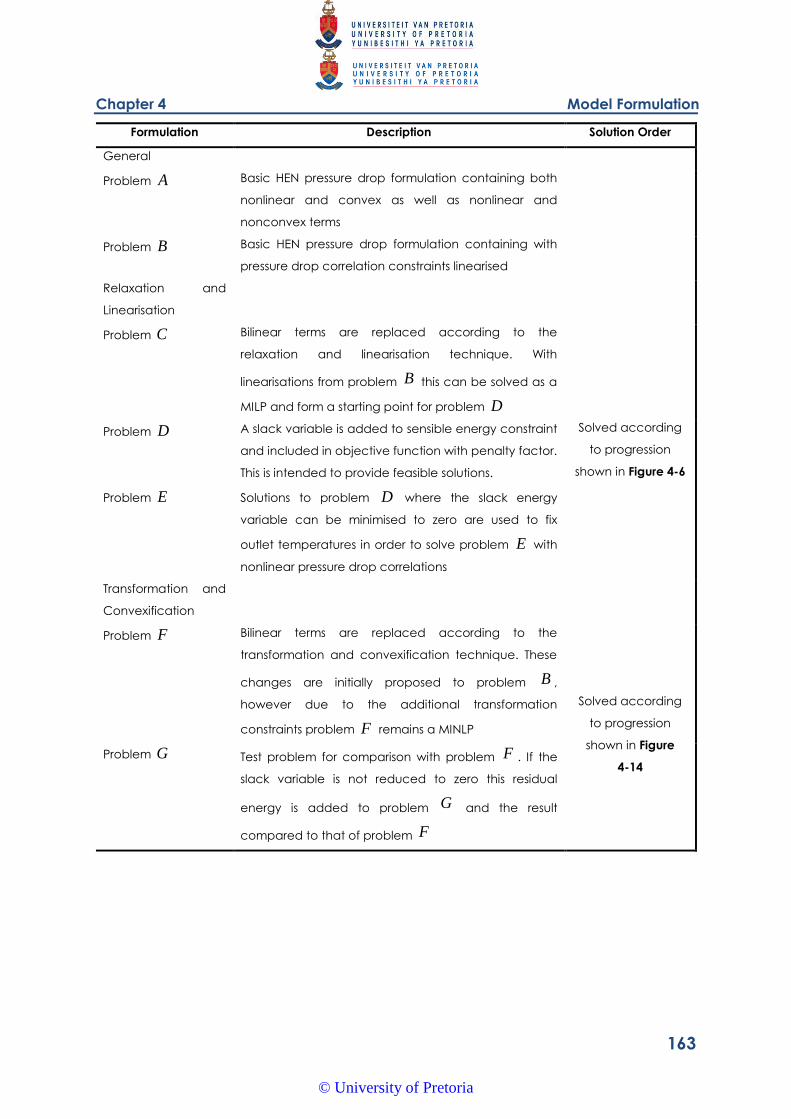
Chapter 4 Model Formulation
163
Formulation Description Solution Order
General
Problem A Basic HEN pressure drop formulation containing both
nonlinear and convex as well as nonlinear and
nonconvex terms
Problem B Basic HEN pressure drop formulation containing with
pressure drop correlation constraints linearised
Relaxation and
Linearisation
Problem C Bilinear terms are replaced according to the
relaxation and linearisation technique. With
linearisations from problem B this can be solved as a
MILP and form a starting point for problem D
Solved according
to progression
shown in Figure 4-6
Problem D A slack variable is added to sensible energy constraint
and included in objective function with penalty factor.
This is intended to provide feasible solutions.
Problem E Solutions to problem D where the slack energy
variable can be minimised to zero are used to fix
outlet temperatures in order to solve problem E with
nonlinear pressure drop correlations
Transformation and
Convexification
Problem F Bilinear terms are replaced according to the
transformation and convexification technique. These
changes are initially proposed to problem B ,
however due to the additional transformation
constraints problem F remains a MINLP
Solved according
to progression
shown in Figure
4-14 Problem G Test problem for comparison with problem F . If the
slack variable is not reduced to zero this residual
energy is added to problem G and the result
compared to that of problem F
© University of Pretoria
Chapter 4 Model Formulation
164
4.10. References
Coetzee, W.A. and Majozi, T. (2008) Steam System Network Design Using Process
Integration, Industrial Engineering Chemistry Research 2008, 47, 4405-4413.
Kim, J. K. and Smith, R. (2003) Automated retrofit design of cooling-water systems,
Process Systems Engineering, Vol 49, No7, pages 1712-1730.
Gass, S. I. (1985) Linear Programming, 5th Edition, Mcgraw-Hill, New York.
Glover, F. (1975) Improved linear integer programming formulation of nonlinear
problems, Management Science, Pages 455-460.
Kocis, G. R. and Grossmann, I. E. (1989) A Modelling and Decomposition Strategy for
MINLP Optimization of Process Flowsheets, Computers and Chemical Engineering ,
13 (7), 797-819.
Price, T. and Majozi, T. (2010a) On Synthesis and Optimization of Steam System
Networks. 1. Sustained Boiler Efficiency. Industrial Engineering Chemistry Research 49
, 9143–9153.
Price, T. and Majozi, T. (2010c) On Synthesis and Optimization of Steam System
Networks. 3. Pressure Drop Consideration. Industrial Engineering Chemistry Research
49 , 9165–9174.
Peters, M. S. and Timmerhaus, K. D. (1991) Plant design and economics for chemical
engineers, 4th Edition, Mcgraw-Hill, New York.
Pörn, R., Bjork, K., and Westerlund, T. (2008) Global solution of optimization problems
with signomial parts. Discrete Optimization 5 , 108-120.
Pörn, R. Harjunkoski, I. and Westerlund, T. (1999) Convexification of different classes of
nonconvex MINLP problems. Computers and Chemical Engineering 23 , 439-448.
Savelski, M. J. and Bagajewicz, M. J. (2000) On the optimality conditions of water
utilization systems in process plants with single contaminants, Chemical Engineering
Science 55, pages 5035-5048.
© University of Pretoria
Chapter 4 Model Formulation
165
© University of Pretoria
Chapter 5 Case Studies
166
5. Case Studies
This chapter is intended to apply the degenerate HEN optimisation problem in order
to minimise pressure drop and maintain boiler efficiency.
Firstly an analysis of the pressure drop problem portrayed by Price and Majozi
(2010c) where the original base case study information from Coetzee and Majozi
(2008) is described, then the minimum pressure drop solution first described by Price
and Majozi (2010c) is analysed and compared to the solution found by applying the
techniques described in Chapter 4. The degenerate solution formulations are then
used to solve the pressure drop minimisation problem and the solutions are
presented. The most effective solution procedure will then be tested on an
additional case study.
The degenerate solution methodology will then be applied to a system where an
attempt is made to maintain boiler efficiency with less steam, as discussed in
Chapter 4.
5.1. Case Study HEN
The limiting temperature data and duties for the utility streams are shown in Table
5-1. The process streams originate from a petrochemical company where steam at
a single pressure level is supplied and is required to satisfy the duties and adhere to
the limiting temperature constraints. Table 5-1 also shows the minimum steam
flowrate required to satisfy the duty with latent heat. Table 5-2 shows information
relevant to the steam available to the system.
© University of Pretoria
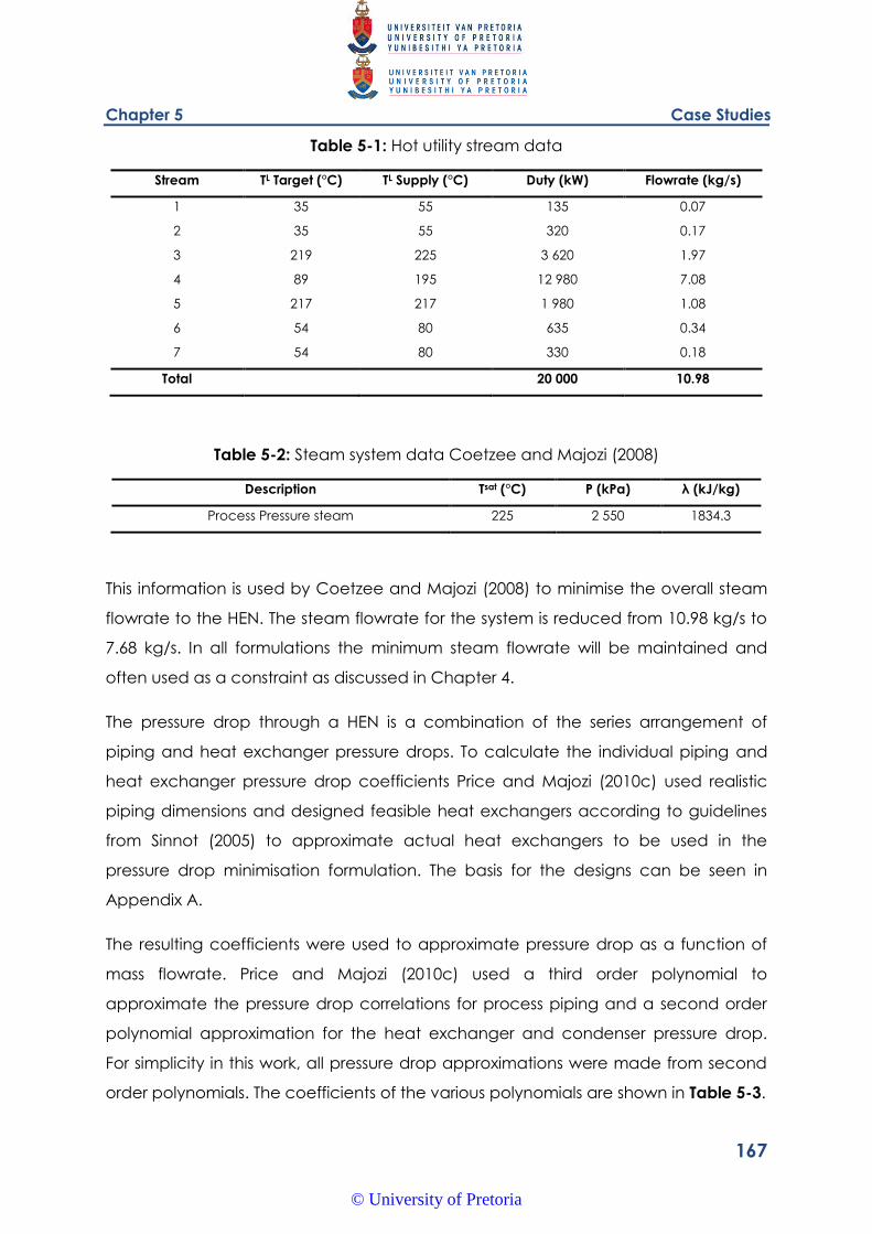
Chapter 5 Case Studies
167
Table 5-1: Hot utility stream data
Stream TL Target (°C) TL Supply (°C) Duty (kW) Flowrate (kg/s)
1 35 55 135 0.07
2 35 55 320 0.17
3 219 225 3 620 1.97
4 89 195 12 980 7.08
5 217 217 1 980 1.08
6 54 80 635 0.34
7 54 80 330 0.18
Total 20 000 10.98
Table 5-2: Steam system data Coetzee and Majozi (2008)
Description Tsat (°C) P (kPa) λ (kJ/kg)
Process Pressure steam 225 2 550 1834.3
This information is used by Coetzee and Majozi (2008) to minimise the overall steam
flowrate to the HEN. The steam flowrate for the system is reduced from 10.98 kg/s to
7.68 kg/s. In all formulations the minimum steam flowrate will be maintained and
often used as a constraint as discussed in Chapter 4.
The pressure drop through a HEN is a combination of the series arrangement of
piping and heat exchanger pressure drops. To calculate the individual piping and
heat exchanger pressure drop coefficients Price and Majozi (2010c) used realistic
piping dimensions and designed feasible heat exchangers according to guidelines
from Sinnot (2005) to approximate actual heat exchangers to be used in the
pressure drop minimisation formulation. The basis for the designs can be seen in
Appendix A.
The resulting coefficients were used to approximate pressure drop as a function of
mass flowrate. Price and Majozi (2010c) used a third order polynomial to
approximate the pressure drop correlations for process piping and a second order
polynomial approximation for the heat exchanger and condenser pressure drop.
For simplicity in this work, all pressure drop approximations were made from second
order polynomials. The coefficients of the various polynomials are shown in Table 5-3.
© University of Pretoria
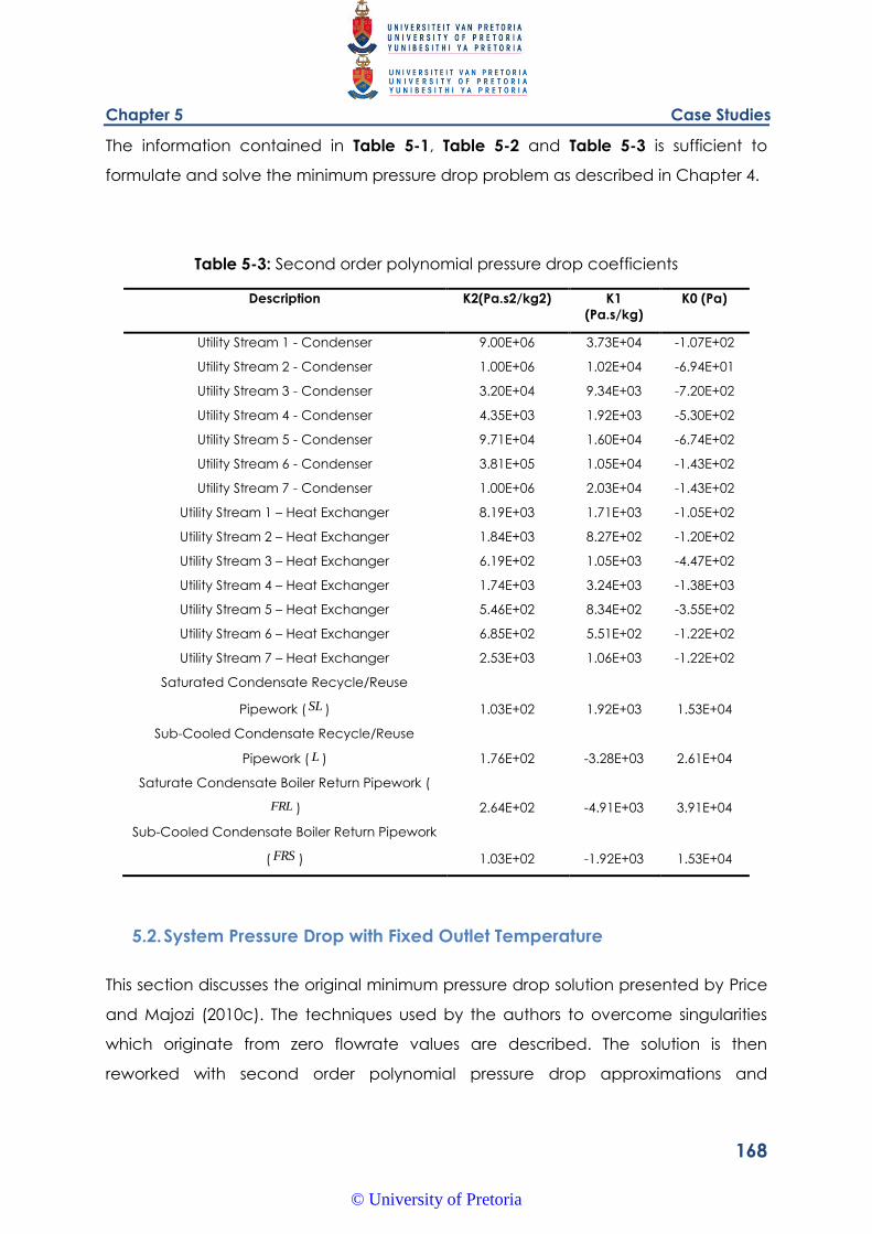
Chapter 5 Case Studies
168
The information contained in Table 5-1, Table 5-2 and Table 5-3 is sufficient to
formulate and solve the minimum pressure drop problem as described in Chapter 4.
Table 5-3: Second order polynomial pressure drop coefficients
Description K2(Pa.s2/kg2) K1
(Pa.s/kg)
K0 (Pa)
Utility Stream 1 - Condenser 9.00E+06 3.73E+04 -1.07E+02
Utility Stream 2 - Condenser 1.00E+06 1.02E+04 -6.94E+01
Utility Stream 3 - Condenser 3.20E+04 9.34E+03 -7.20E+02
Utility Stream 4 - Condenser 4.35E+03 1.92E+03 -5.30E+02
Utility Stream 5 - Condenser 9.71E+04 1.60E+04 -6.74E+02
Utility Stream 6 - Condenser 3.81E+05 1.05E+04 -1.43E+02
Utility Stream 7 - Condenser 1.00E+06 2.03E+04 -1.43E+02
Utility Stream 1 – Heat Exchanger 8.19E+03 1.71E+03 -1.05E+02
Utility Stream 2 – Heat Exchanger 1.84E+03 8.27E+02 -1.20E+02
Utility Stream 3 – Heat Exchanger 6.19E+02 1.05E+03 -4.47E+02
Utility Stream 4 – Heat Exchanger 1.74E+03 3.24E+03 -1.38E+03
Utility Stream 5 – Heat Exchanger 5.46E+02 8.34E+02 -3.55E+02
Utility Stream 6 – Heat Exchanger 6.85E+02 5.51E+02 -1.22E+02
Utility Stream 7 – Heat Exchanger 2.53E+03 1.06E+03 -1.22E+02
Saturated Condensate Recycle/Reuse
Pipework ( SL ) 1.03E+02 1.92E+03 1.53E+04
Sub-Cooled Condensate Recycle/Reuse
Pipework ( L ) 1.76E+02 -3.28E+03 2.61E+04
Saturate Condensate Boiler Return Pipework (
FRL ) 2.64E+02 -4.91E+03 3.91E+04
Sub-Cooled Condensate Boiler Return Pipework
( FRS ) 1.03E+02 -1.92E+03 1.53E+04
5.2. System Pressure Drop with Fixed Outlet Temperature
This section discusses the original minimum pressure drop solution presented by Price
and Majozi (2010c). The techniques used by the authors to overcome singularities
which originate from zero flowrate values are described. The solution is then
reworked with second order polynomial pressure drop approximations and
© University of Pretoria
Chapter 5 Case Studies
169
translations to overcome the singularities. The formulation is then linearised as
discussed in Section 4.3.2 so as to approximate a globally optimal solution.
5.2.1. Solution from Price and Majozi (2010c)
Price and Majozi (2010c) used the flowrate minimisation model derived in Price and
Majozi (2010a) along with the pressure drop correlations shown in Chapter 4. As in
Price and Majozi (2010a) the boiler efficiency for the case study was also
maintained. This is done in Price and Majozi (2010c) by first solving for the relevant
minimum steam flowrate that is able to maintain the boiler efficiency and then
utilising this flowrate in the pressure minimisation model.
The formulation contains mixed integer terms as well as non linear terms making the
pressure drop minimisation formulation an MINLP. The MINLP solver DICOPT was
utilised in the optimisation software package GAMS.
The problem formulation in GAMS required some minor adjustments to the basic
constraints presented in Chapter 4. These are as a result of singularities that occur
when the steam or condensate flowrate is zero in nonlinear terms. The nonlinear
terms in question are cubic and square terms in the polynomial representations of
pressure drop through heat exchangers and pipework. In GAMS, an exponentiation
such as a square or cubic function is calculated as xn ln.exp where n is the
exponent and x is the variable. The natural logarithm of zero is undefined in GAMS
and causes errors in NLP solvers. As a large number of the possible heat exchangers
and pipework connections in the heat exchanger network will not necessarily exist in
the final solution the flowrates through these elements can be zero. This has the
potential to cause singularities in the model resulting in model failures.
The technique utilised by Price and Majozi (2010c) was to shift the flowrates to non-
existent heat exchangers and pipework connections away from zero by a small
amount, a value of 0.0001 kg/s. This results in several constraint changes as well as a
relaxation of the minimum steam flowrate to accommodate the offset values.
Representative constraints such as Constraints ( 4.42 ) and ( 4.43 ) are changed as
shown in Constraints ( 5-1 ) and ( 5-2 )
© University of Pretoria
Chapter 5 Case Studies
170
0001.010001.0 SLSLU yySLSL ( 5-1 )
0001.010001.0 SLSLL yySLSL ( 5-2 )
Using the changes above the minimum steam flowrate was then relaxed until a
feasible solution was found in using the DICOPT MINLP algorithm in GAMS. A feasible
pressure drop was found using a flowrate relaxation of 0.0405 kg/s, a relaxation of
less than 1% of the minimum steam flowrate of 7.6806 kg/s. The pressure drop
calculated using this relaxation is reported in Price and Majozi (2010c) as 344.40 kPa.
Optimality of solutions
The DICOPT solver can guarantee global optimality of solutions providing the
nonlinear constraints are convex or quasi-convex within the feasible region (Kocis
and Grossmann, 1989). The exponential functions used to represent pressure drop
are nonconvex in the range of the mass flowrate. Therefore the global optimality of
the solution found by Price and Majozi (2010c) cannot be guaranteed.
5.2.2. Solution with Exact Minimum Steam Flowrate
Several improvements to the formulation used by Price and Majozi (2010c) can be
implemented in an attempt to attain a better solution. The first is to completely
remove the possibility of singularities by creating a dummy variable to replace the
nonlinear exponentials functions. This will allow a more effective shift of the operating
area away from the singularities created by zero flows. The removal of binary
variables from functions involving other variables can also improve the solution
procedure of DICOPT Kocis and Grossmann (1989).
The first improvement is accomplished using translations as discussed in Section 4.3.1.
This effectively removes the singularities from the formulation, removing errors when
any of the variables involved in nonlinear functions approach zero. A further
improvement is the removal of binary variables from constraints where other
variables appear. This is discussed in more detail in Section 4.6.
© University of Pretoria
Chapter 5 Case Studies
171
5.2.3. Reworked Formulations
The replacement of third order polynomials as discussed in Section 4.2.2 will require
the original optimum pressure drop calculated by Price and Majozi (2010c) to be
recalculated using the square polynomial approximations. This was completed and
the minimum pressure drop found when not restricting the number of split heat
exchangers was 413.38 kPa using the technique of Price and Majozi (2010c). By
individually varying the heat exchanger splits the minimum pressure drop was found
to be 321.21 kPa with two heat exchanger splits.
Using the techniques demonstrated above the pressure drop can be slightly
reduced to 321.18 kPa using the same mass flowrate relaxation. The formulations did
however make it possible to find a minimum pressure drop without the need to relax
the mass flowrate at all. Using the minimum flowrate found in Price and Majozi
(2010c) the minimum pressure drop was calculated as 364,43 kPa. This result will be
used for comparison going forward as this is the result obtained using the technique
of Price and Majozi (2010c).
5.2.4. Solution
The flow network for the solution described above is shown in Figure 5-1. All flowrates
are reported in kg/s.
© University of Pretoria
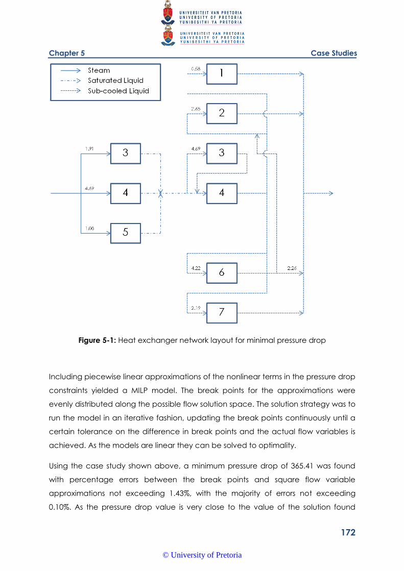
Chapter 5 Case Studies
172
Figure 5-1: Heat exchanger network layout for minimal pressure drop
Including piecewise linear approximations of the nonlinear terms in the pressure drop
constraints yielded a MILP model. The break points for the approximations were
evenly distributed along the possible flow solution space. The solution strategy was to
run the model in an iterative fashion, updating the break points continuously until a
certain tolerance on the difference in break points and the actual flow variables is
achieved. As the models are linear they can be solved to optimality.
Using the case study shown above, a minimum pressure drop of 365.41 was found
with percentage errors between the break points and square flow variable
approximations not exceeding 1.43%, with the majority of errors not exceeding
0.10%. As the pressure drop value is very close to the value of the solution found
© University of Pretoria
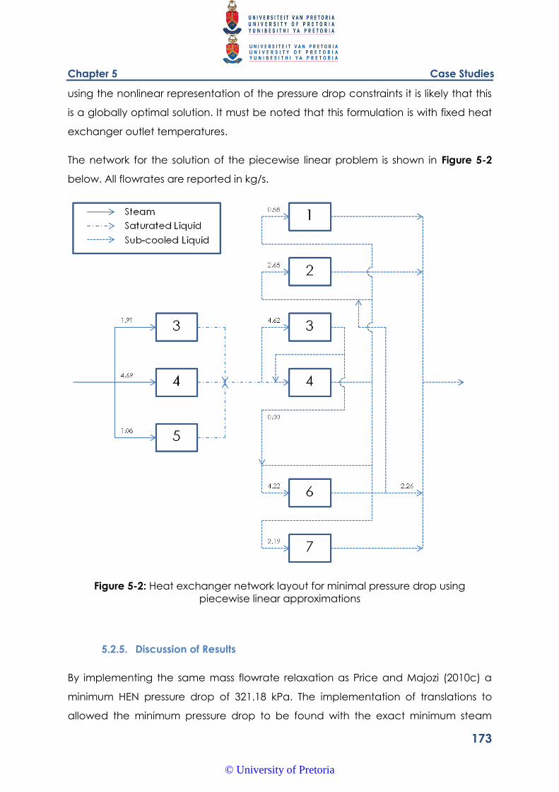
Chapter 5 Case Studies
173
using the nonlinear representation of the pressure drop constraints it is likely that this
is a globally optimal solution. It must be noted that this formulation is with fixed heat
exchanger outlet temperatures.
The network for the solution of the piecewise linear problem is shown in Figure 5-2
below. All flowrates are reported in kg/s.
Figure 5-2: Heat exchanger network layout for minimal pressure drop using
piecewise linear approximations
5.2.5. Discussion of Results
By implementing the same mass flowrate relaxation as Price and Majozi (2010c) a
minimum HEN pressure drop of 321.18 kPa. The implementation of translations to
allowed the minimum pressure drop to be found with the exact minimum steam
© University of Pretoria
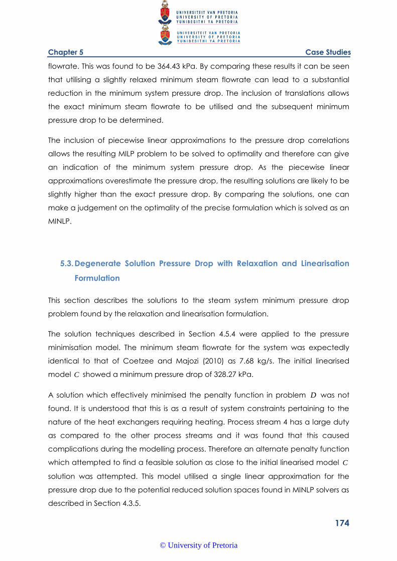
Chapter 5 Case Studies
174
flowrate. This was found to be 364.43 kPa. By comparing these results it can be seen
that utilising a slightly relaxed minimum steam flowrate can lead to a substantial
reduction in the minimum system pressure drop. The inclusion of translations allows
the exact minimum steam flowrate to be utilised and the subsequent minimum
pressure drop to be determined.
The inclusion of piecewise linear approximations to the pressure drop correlations
allows the resulting MILP problem to be solved to optimality and therefore can give
an indication of the minimum system pressure drop. As the piecewise linear
approximations overestimate the pressure drop, the resulting solutions are likely to be
slightly higher than the exact pressure drop. By comparing the solutions, one can
make a judgement on the optimality of the precise formulation which is solved as an
MINLP.
5.3. Degenerate Solution Pressure Drop with Relaxation and Linearisation
Formulation
This section describes the solutions to the steam system minimum pressure drop
problem found by the relaxation and linearisation formulation.
The solution techniques described in Section 4.5.4 were applied to the pressure
minimisation model. The minimum steam flowrate for the system was expectedly
identical to that of Coetzee and Majozi (2010) as 7.68 kg/s. The initial linearised
model C showed a minimum pressure drop of 328.27 kPa.
A solution which effectively minimised the penalty function in problem D was not
found. It is understood that this is as a result of system constraints pertaining to the
nature of the heat exchangers requiring heating. Process stream 4 has a large duty
as compared to the other process streams and it was found that this caused
complications during the modelling process. Therefore an alternate penalty function
which attempted to find a feasible solution as close to the initial linearised model C
solution was attempted. This model utilised a single linear approximation for the
pressure drop due to the potential reduced solution spaces found in MINLP solvers as
described in Section 4.3.5.
© University of Pretoria
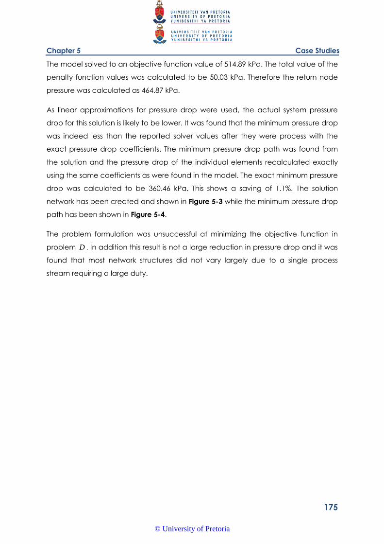
Chapter 5 Case Studies
175
The model solved to an objective function value of 514.89 kPa. The total value of the
penalty function values was calculated to be 50.03 kPa. Therefore the return node
pressure was calculated as 464.87 kPa.
As linear approximations for pressure drop were used, the actual system pressure
drop for this solution is likely to be lower. It was found that the minimum pressure drop
was indeed less than the reported solver values after they were process with the
exact pressure drop coefficients. The minimum pressure drop path was found from
the solution and the pressure drop of the individual elements recalculated exactly
using the same coefficients as were found in the model. The exact minimum pressure
drop was calculated to be 360.46 kPa. This shows a saving of 1.1%. The solution
network has been created and shown in Figure 5-3 while the minimum pressure drop
path has been shown in Figure 5-4.
The problem formulation was unsuccessful at minimizing the objective function in
problem D . In addition this result is not a large reduction in pressure drop and it was
found that most network structures did not vary largely due to a single process
stream requiring a large duty.
© University of Pretoria
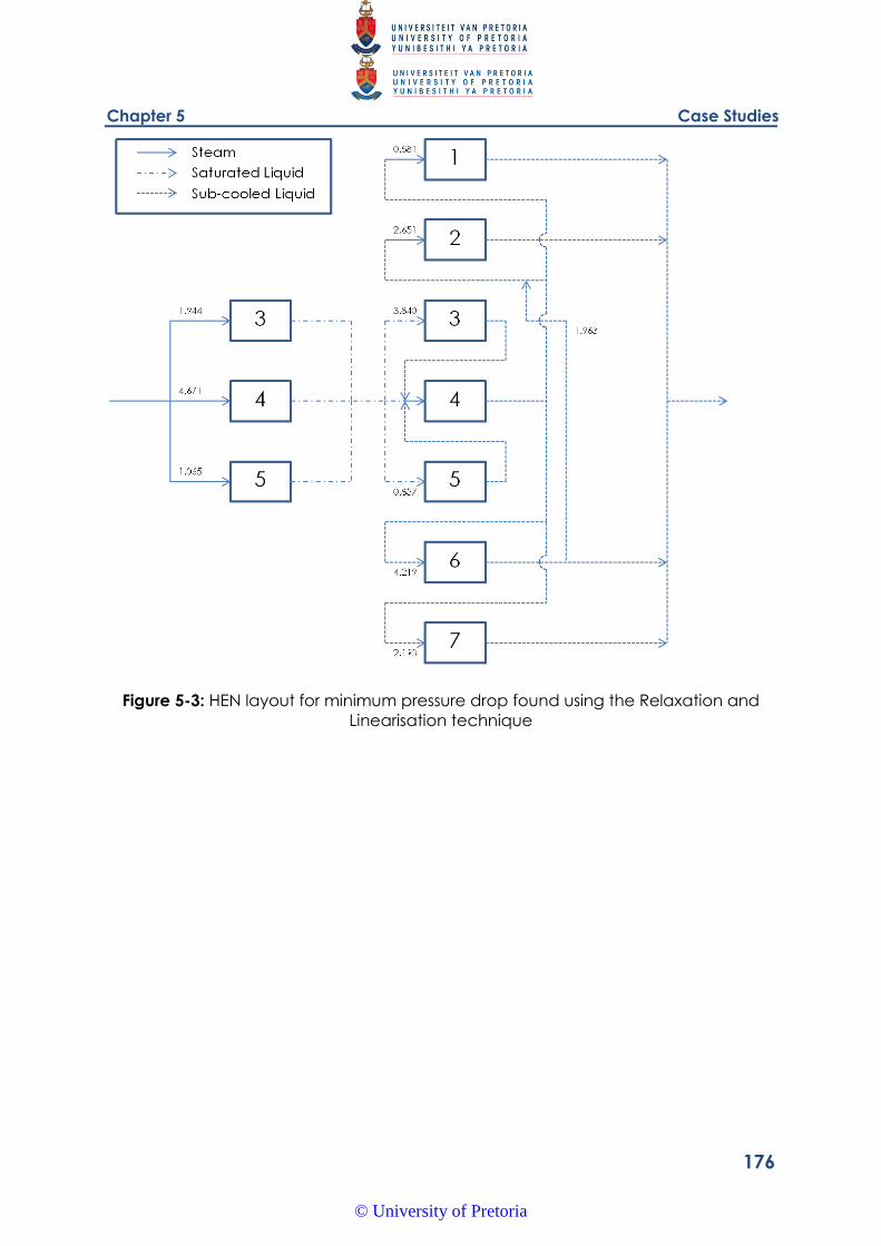
Chapter 5 Case Studies
176
Figure 5-3: HEN layout for minimum pressure drop found using the Relaxation and
Linearisation technique
© University of Pretoria
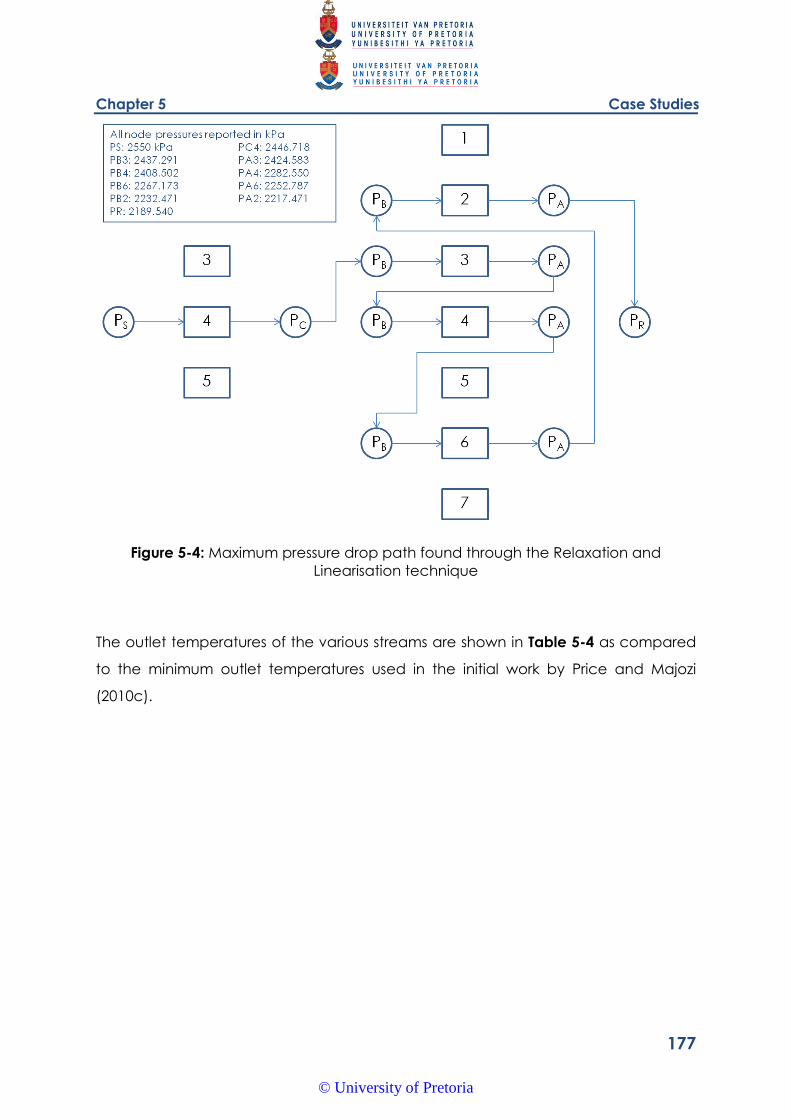
Chapter 5 Case Studies
177
Figure 5-4: Maximum pressure drop path found through the Relaxation and
Linearisation technique
The outlet temperatures of the various streams are shown in Table 5-4 as compared
to the minimum outlet temperatures used in the initial work by Price and Majozi
(2010c).
© University of Pretoria
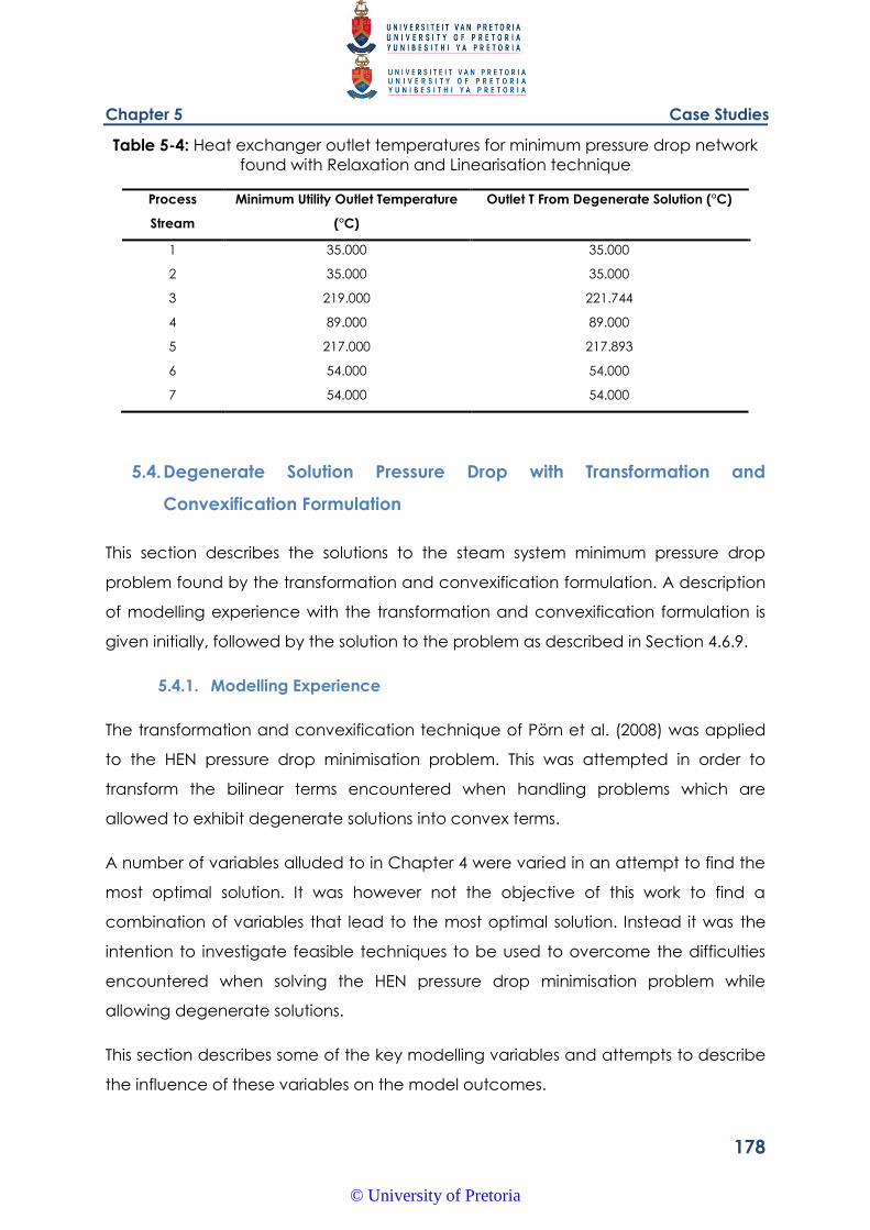
Chapter 5 Case Studies
178
Table 5-4: Heat exchanger outlet temperatures for minimum pressure drop network
found with Relaxation and Linearisation technique
Process
Stream
Minimum Utility Outlet Temperature
(°C)
Outlet T From Degenerate Solution (°C)
1 35.000 35.000
2 35.000 35.000
3 219.000 221.744
4 89.000 89.000
5 217.000 217.893
6 54.000 54.000
7 54.000 54.000
5.4. Degenerate Solution Pressure Drop with Transformation and
Convexification Formulation
This section describes the solutions to the steam system minimum pressure drop
problem found by the transformation and convexification formulation. A description
of modelling experience with the transformation and convexification formulation is
given initially, followed by the solution to the problem as described in Section 4.6.9.
5.4.1. Modelling Experience
The transformation and convexification technique of Pörn et al. (2008) was applied
to the HEN pressure drop minimisation problem. This was attempted in order to
transform the bilinear terms encountered when handling problems which are
allowed to exhibit degenerate solutions into convex terms.
A number of variables alluded to in Chapter 4 were varied in an attempt to find the
most optimal solution. It was however not the objective of this work to find a
combination of variables that lead to the most optimal solution. Instead it was the
intention to investigate feasible techniques to be used to overcome the difficulties
encountered when solving the HEN pressure drop minimisation problem while
allowing degenerate solutions.
This section describes some of the key modelling variables and attempts to describe
the influence of these variables on the model outcomes.
© University of Pretoria
Chapter 5 Case Studies
179
Number of Tangents
The number of tangents used to approximate the nonlinear terms in the ET and PT
can be varied. A larger number of tangents will lead to a closer approximation of
the natural logarithm and square functions found in the ET and PT respectively.
However the drawback of a large number of tangents is the large number of
associated binary variables which need to be assigned to activate a particular
tangent. These binary variables can be built into the formulation manually or if an
MILP solver is capable of using SOS2 variables these can be used instead. This is
discussed further in Section 4.3.5.
By utilising a branch and bound type MINLP solver, binary variables are fixed
between the master MILP and nonlinear sub problems. By fixing binary variables only
a certain portion of the solution space is available for the nonlinear sub problem to
find a solution. This could negatively impact the final solution.
To ensure a larger solution space, initially low numbers of tangents were chosen
ranging between 1 and 4. These solutions were then compared to larger numbers of
tangents and it was found that solution spaces divided by between 5 and 10
tangents exhibited the best mix of solution time for the MILP master problem and
feasible solutions in the NLP problems.
More powerful processors will likely be able to cater for larger numbers of tangents
and the optimal number of tangents could be made a further field of investigation.
Slack Variable Penalty Constants
Slack variables are used to make the solution values tend closer to tangential points
as shown in Section 4.6.6. These slack variables are intended to allow individual
solutions to vary from the tangential points, however the iterative updating of
tangential points is intended to find a solution.
The penalty constants assigned to the slack variables were attempted in a number
of different ways. Initially a linear penalty constant where each heating stream i was
penalised by a constant in the range of 0.1 to 10 was implemented. It was then
found that varying the penalty constant based on the duty of the heating stream
(where higher duty streams were penalised less) was implemented. This was
© University of Pretoria
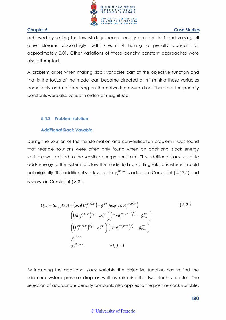
Chapter 5 Case Studies
180
achieved by setting the lowest duty stream penalty constant to 1 and varying all
other streams accordingly, with stream 4 having a penalty constant of
approximately 0.01. Other variations of these penalty constant approaches were
also attempted.
A problem arises when making slack variables part of the objective function and
that is the focus of the model can become directed at minimising these variables
completely and not focussing on the network pressure drop. Therefore the penalty
constants were also varied in orders of magnitude.
5.4.2. Problem solution
Additional Slack Variable
During the solution of the transformation and convexification problem it was found
that feasible solutions were often only found when an additional slack energy
variable was added to the sensible energy constraint. This additional slack variable
adds energy to the system to allow the model to find starting solutions where it could
not originally. This additional slack variable posSE
i
, is added to Constraint ( 4.122 ) and
is shown in Constraint ( 5-3 ).
Iji
ToutL
ToutSL
ToutLTsatSLQL
posSE
i
negSE
i
PT
Tout
PLTPT
i
PT
L
PLTPT
ij
PT
Tout
PLTPT
i
PT
SL
PLTPT
ij
PLTET
j
ET
L
PLTET
ijiji
,
expexp
,
,
21
,21
,
,
21
,21
,
,
,,
,,
( 5-3 )
By including the additional slack variable the objective function has to find the
minimum system pressure drop as well as minimise the two slack variables. The
selection of appropriate penalty constants also applies to the positive slack variable.
© University of Pretoria
Chapter 5 Case Studies
181
This variable essentially represents free energy and should therefore be heavily
penalised for any use.
Both Constraint ( 4.122 ) and Constraint ( 4.122 ) were utilised to solve problem F .
Many attempts to solve problem F were made with varying numbers of tangents.
Many solutions of the pseudo exact problem revealed problem F having a better
solution than problem G , but processing of the exact solution revealed the problem
G solution to be better.
Solution Variants
Different numbers of tangents were utilised in an attempt to find solutions to problem
F that showed an improved pressure drop to problem G . Solutions were tested with
between 3 and 20 tangents. Those with few tangents typically showed large excess
sensible heat values. Those with high numbers of tangents typically had poorer
solutions which is likely due to restrictions on solution time. The most successful
numbers of tangents ranged between 5 and 10 and solutions to these will be
discussed.
The most successful solution using 5 tangents utilised Constraint ( 4.122 ) and
exhibited penalty functions that varied according to the required duty of the various
heat exchangers. . Problem F was solved to a pressure drop of 277.883 kPa. After
processing, this solution was found to be 209.202 kPa. The initial solution to problem
G was found to be 279.245 kPa and after processing was found to be 208.152 kPa.
This solution shows the pressure drop for problem F to be higher than for problem G
by 1.050 kPa.
The smallest difference between problem F and problem G was found from a
model with 10 tangents utilising Constraint ( 4.122 ) and having the penalty functions
vary according to the required duty of the various heat exchangers. Problem F was
solved to a pressure drop of 282.788 kPa. After processing, this solution was found to
be 211.525 kPa. The initial solution to problem G was found to be 287.187 kPa and
after processing was found to be 210.994 kPa. This solution shows the pressure drop
for problem F to be higher than for problem G by 0.531 kPa.
© University of Pretoria
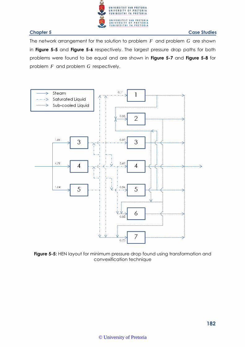
Chapter 5 Case Studies
182
The network arrangement for the solution to problem F and problem G are shown
in Figure 5-5 and Figure 5-6 respectively. The largest pressure drop paths for both
problems were found to be equal and are shown in Figure 5-7 and Figure 5-8 for
problem F and problem G respectively.
Figure 5-5: HEN layout for minimum pressure drop found using transformation and
convexification technique
© University of Pretoria
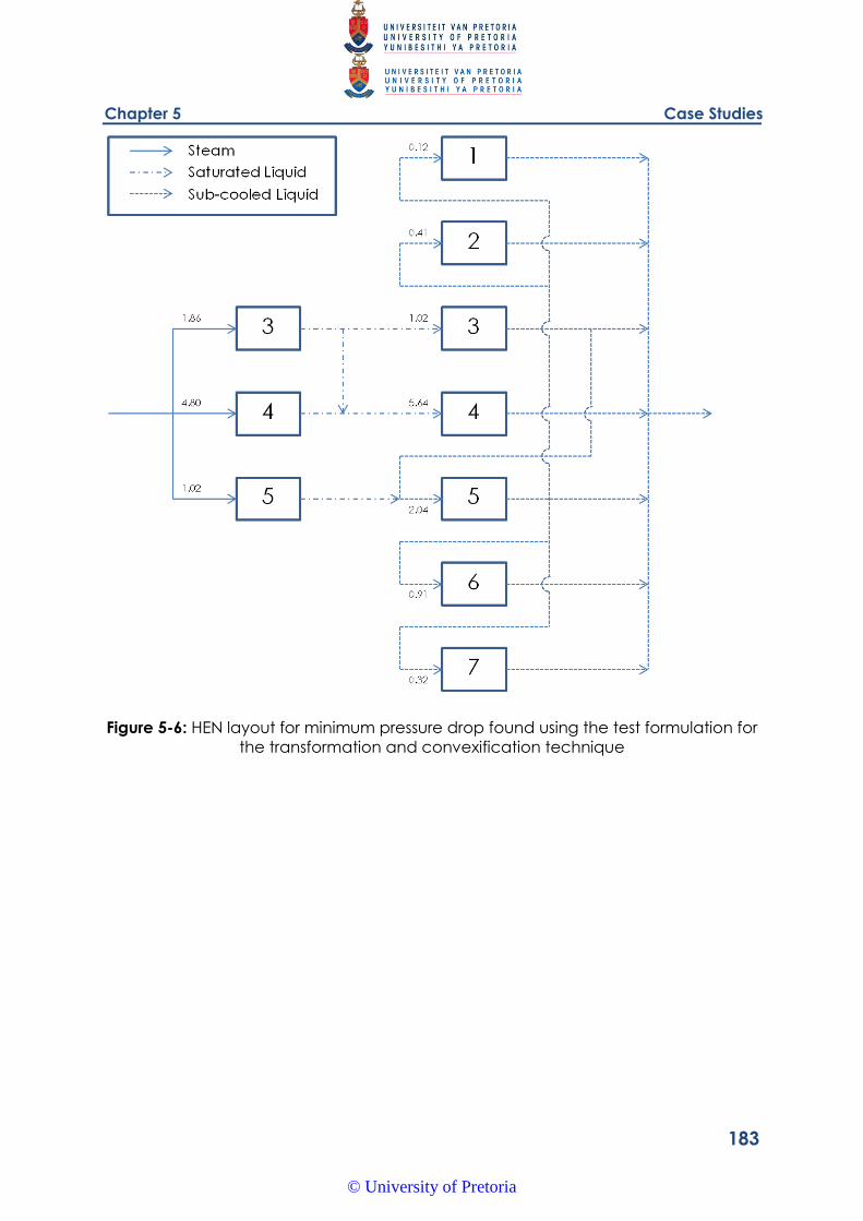
Chapter 5 Case Studies
183
Figure 5-6: HEN layout for minimum pressure drop found using the test formulation for
the transformation and convexification technique
© University of Pretoria
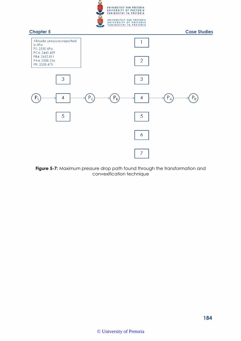
Chapter 5 Case Studies
184
Figure 5-7: Maximum pressure drop path found through the transformation and
convexification technique
© University of Pretoria
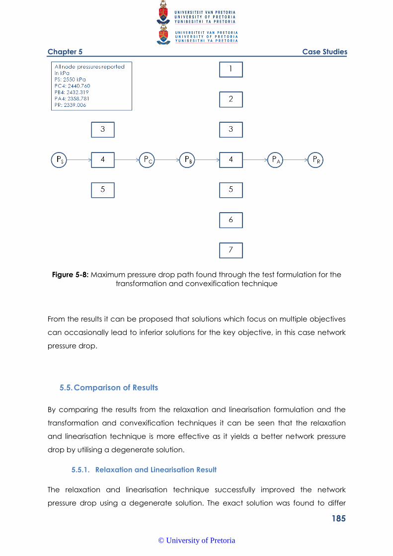
Chapter 5 Case Studies
185
Figure 5-8: Maximum pressure drop path found through the test formulation for the
transformation and convexification technique
From the results it can be proposed that solutions which focus on multiple objectives
can occasionally lead to inferior solutions for the key objective, in this case network
pressure drop.
5.5. Comparison of Results
By comparing the results from the relaxation and linearisation formulation and the
transformation and convexification techniques it can be seen that the relaxation
and linearisation technique is more effective as it yields a better network pressure
drop by utilising a degenerate solution.
5.5.1. Relaxation and Linearisation Result
The relaxation and linearisation technique successfully improved the network
pressure drop using a degenerate solution. The exact solution was found to differ
© University of Pretoria
Chapter 5 Case Studies
186
from the relaxed solution, therefore the global optimality of the solution presented
cannot be guaranteed.
5.5.2. Transformation and Convexification Result
The transformation and convexification technique fails to yield a better pressure
drop than a solution found utilising the fixed outlet temperature approach of Savelski
and Bagajewicz (2000). Furthermore this technique requires overestimation of the
sensible energy terms. This will require additional design work to create a feasible
HEN. The transformation and convexification technique of Pörn et al. (2008) is
effective at solving MINLP problems, however it was found that this technique had
difficulty being used alongside the critical path algorithm. This caused the objective
function of problem F to minimise pressure drop along with slack variables. This
trade off proved to be less effective than the pure pressure drop objective function
utilised when the outlet temperatures were fixed.
It is likely that the manipulations employed in the transformation and convexification
methodology presented in this work can be improved upon and this could be the
basis of further research.
5.5.3. Conclusion
The outlet temperature of heat exchangers can be allowed to vary in an attempt to
further reduce the pressure drop through a HEN. It was found that these degenerate
solutions can successfully be used to reduce the pressure drop through a HEN as
compared to a network where the outlet temperatures of the individual heat
exchangers are fixed to their minimum values.
The relaxation and linearisation technique was found to successfully improve the
HEN network pressure drop using a degenerate solution. This was done by
overcoming the complications of a nonconvex MINLP problem utilising a technique
successfully employed in literature. As the transformation and convexification
technique was unable to find an improved solution, the relaxation and linearisation
technique was found to be the most effective.
© University of Pretoria
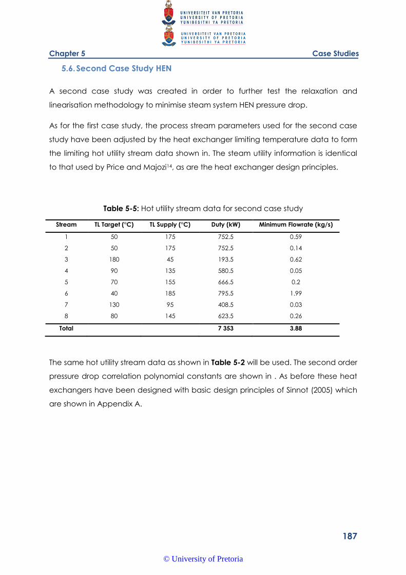
Chapter 5 Case Studies
187
5.6. Second Case Study HEN
A second case study was created in order to further test the relaxation and
linearisation methodology to minimise steam system HEN pressure drop.
As for the first case study, the process stream parameters used for the second case
study have been adjusted by the heat exchanger limiting temperature data to form
the limiting hot utility stream data shown in. The steam utility information is identical
to that used by Price and Majozi14, as are the heat exchanger design principles.
Table 5-5: Hot utility stream data for second case study
Stream TL Target (°C) TL Supply (°C) Duty (kW) Minimum Flowrate (kg/s)
1 50 175 752.5 0.59
2 50 175 752.5 0.14
3 180 45 193.5 0.62
4 90 135 580.5 0.05
5 70 155 666.5 0.2
6 40 185 795.5 1.99
7 130 95 408.5 0.03
8 80 145 623.5 0.26
Total 7 353 3.88
The same hot utility stream data as shown in Table 5-2 will be used. The second order
pressure drop correlation polynomial constants are shown in . As before these heat
exchangers have been designed with basic design principles of Sinnot (2005) which
are shown in Appendix A.
© University of Pretoria
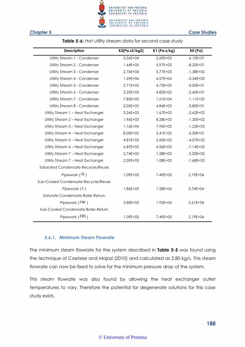
Chapter 5 Case Studies
188
Table 5-6: Hot utility stream data for second case study
Description K2(Pa.s2/kg2) K1 (Pa.s/kg) K0 (Pa)
Utility Stream 1 - Condenser 3.56E+04 2.69E+03 -6.10E+01
Utility Stream 2 - Condenser 1.44E+05 5.97E+03 -8.20E+01
Utility Stream 3 - Condenser 2.76E+04 3.77E+03 -1.38E+02
Utility Stream 4 - Condenser 1.59E+06 4.57E+04 -3.34E+02
Utility Stream 5 - Condenser 2.71E+05 4.73E+03 -3.00E+01
Utility Stream 6 - Condenser 3.23E+03 4.82E+02 -2.60E+01
Utility Stream 7 - Condenser 7.85E+05 1.61E+04 -1.11E+02
Utility Stream 8 - Condenser 2.05E+05 4.84E+03 -3.80E+01
Utility Stream 1 – Heat Exchanger 3.26E+03 1.67E+03 -2.62E+02
Utility Stream 2 – Heat Exchanger 1.96E+03 8.28E+02 -1.30E+02
Utility Stream 3 – Heat Exchanger 1.16E+04 7.95E+03 -1.25E+03
Utility Stream 4 – Heat Exchanger 8.00E+02 3.41E+02 -5.30E+01
Utility Stream 5 – Heat Exchanger 4.81E+03 2.60E+03 -4.07E+02
Utility Stream 6 – Heat Exchanger 6.87E+03 4.56E+03 -7.14E+02
Utility Stream 7 – Heat Exchanger 2.74E+03 1.28E+03 -2.00E+02
Utility Stream 7 – Heat Exchanger 2.09E+03 1.08E+03 -1.68E+02
Saturated Condensate Recycle/Reuse
Pipework ( SL ) 1.09E+03 7.49E+03 2.19E+04
Sub-Cooled Condensate Recycle/Reuse
Pipework ( L ) 1.86E+03 1.28E+04 3.74E+04
Saturate Condensate Boiler Return
Pipework ( FRL ) 2.80E+03 1.92E+04 5.61E+04
Sub-Cooled Condensate Boiler Return
Pipework ( FRS ) 1.09E+03 7.49E+03 2.19E+04
5.6.1. Minimum Steam Flowrate
The minimum steam flowrate for the system described in Table 5-5 was found using
the technique of Coetzee and Majozi (2010) and calculated as 2.80 kg/s. This steam
flowrate can now be fixed to solve for the minimum pressure drop of the system.
This steam flowrate was also found by allowing the heat exchanger outlet
temperatures to vary. Therefore the potential for degenerate solutions for this case
study exists.
© University of Pretoria
Chapter 5 Case Studies
189
5.6.2. System Pressure Drop
Here the system pressure drop was solved for using the fixed heat exchanger outlet
temperatures as well as with allowing the temperatures to vary.
Fixed Heat Exchanger Outlet Temperatures
By fixing the heat exchanger outlet temperatures to minimum described in Table 5-5
the minimum pressure drop for the system was solved to 164.16 kPa.
This value can now be used as a basis for comparison for the degenerate solution.
Variable Heat Exchanger Outlet Temperatures
By allowing the hot utility stream heat exchanger outlet temperatures to vary, a
minimum pressure drop of 151.95 kPa was found. This represents a 7.1% improvement
on the previous solution.
The network flow diagram for this solution is shown in Figure 5-9.
© University of Pretoria
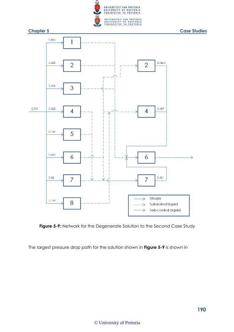
Chapter 5 Case Studies
190
Figure 5-9: Network for the Degenerate Solution to the Second Case Study
The largest pressure drop path for the solution shown in Figure 5-9 is shown in
© University of Pretoria
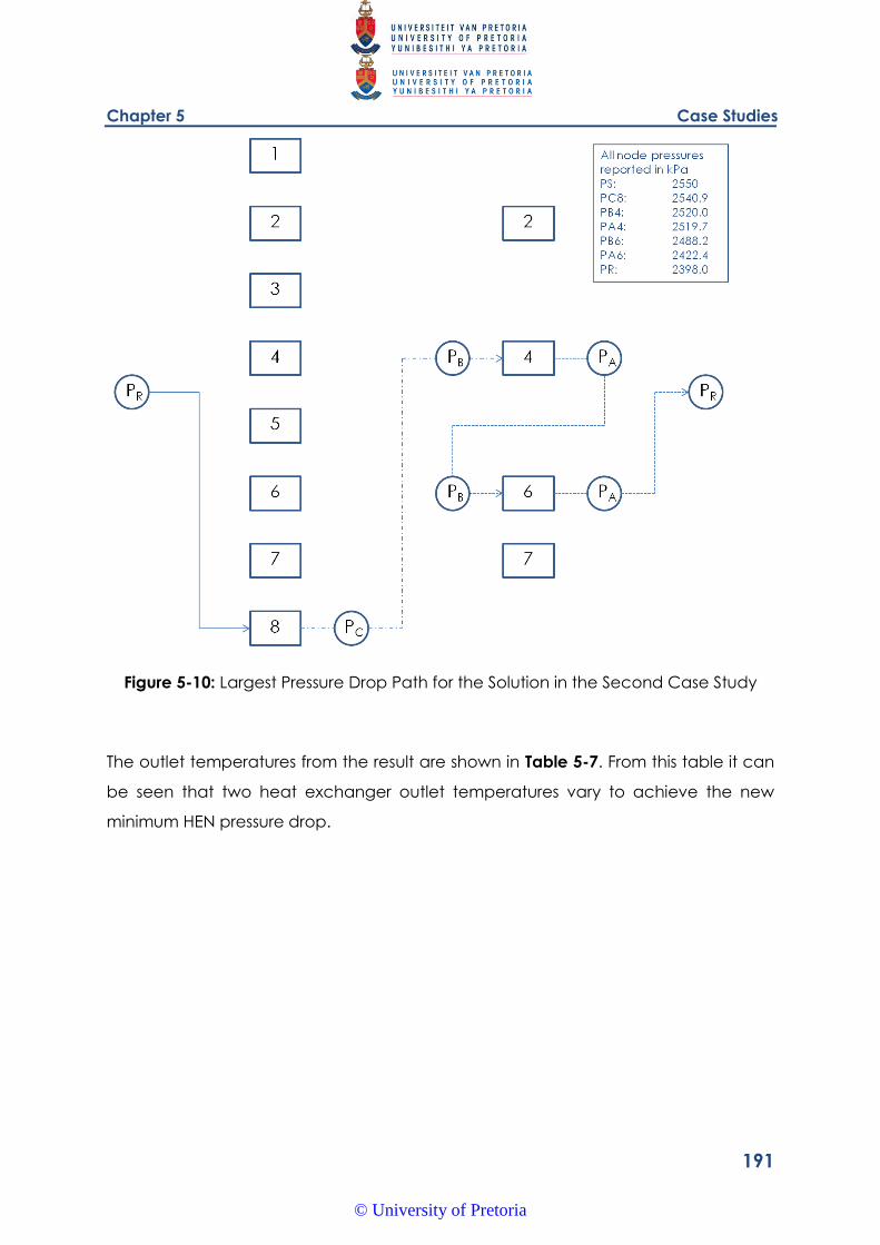
Chapter 5 Case Studies
191
Figure 5-10: Largest Pressure Drop Path for the Solution in the Second Case Study
The outlet temperatures from the result are shown in Table 5-7. From this table it can
be seen that two heat exchanger outlet temperatures vary to achieve the new
minimum HEN pressure drop.
© University of Pretoria
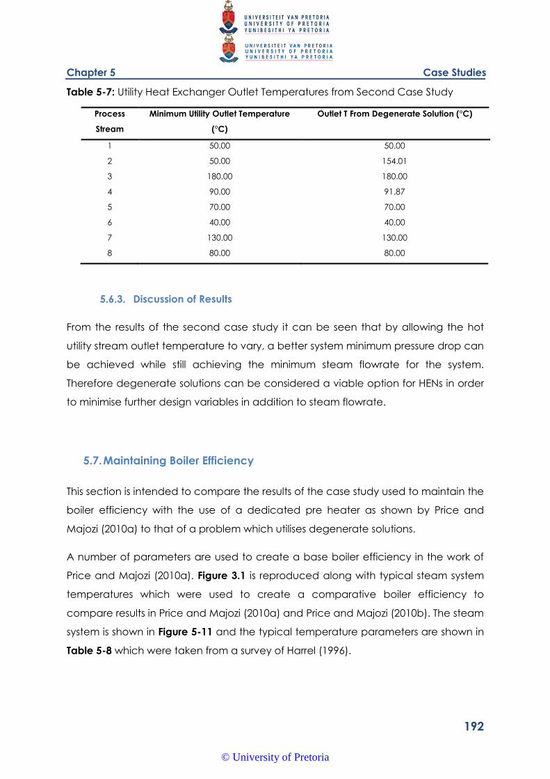
Chapter 5 Case Studies
192
Table 5-7: Utility Heat Exchanger Outlet Temperatures from Second Case Study
Process
Stream
Minimum Utility Outlet Temperature
(°C)
Outlet T From Degenerate Solution (°C)
1 50.00 50.00
2 50.00 154.01
3 180.00 180.00
4 90.00 91.87
5 70.00 70.00
6 40.00 40.00
7 130.00 130.00
8 80.00 80.00
5.6.3. Discussion of Results
From the results of the second case study it can be seen that by allowing the hot
utility stream outlet temperature to vary, a better system minimum pressure drop can
be achieved while still achieving the minimum steam flowrate for the system.
Therefore degenerate solutions can be considered a viable option for HENs in order
to minimise further design variables in addition to steam flowrate.
5.7. Maintaining Boiler Efficiency
This section is intended to compare the results of the case study used to maintain the
boiler efficiency with the use of a dedicated pre heater as shown by Price and
Majozi (2010a) to that of a problem which utilises degenerate solutions.
A number of parameters are used to create a base boiler efficiency in the work of
Price and Majozi (2010a). Figure 3.1 is reproduced along with typical steam system
temperatures which were used to create a comparative boiler efficiency to
compare results in Price and Majozi (2010a) and Price and Majozi (2010b). The steam
system is shown in Figure 5-11 and the typical temperature parameters are shown in
Table 5-8 which were taken from a survey of Harrel (1996).
© University of Pretoria
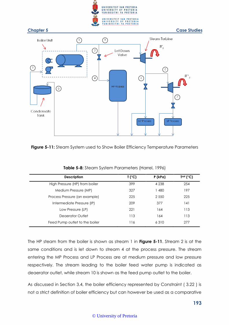
Chapter 5 Case Studies
193
Figure 5-11: Steam System used to Show Boiler Efficiency Temperature Parameters
Table 5-8: Steam System Parameters (Harrel, 1996)
Description T (°C) P (kPa) Tsat (°C)
High Pressure (HP) from boiler 399 4 238 254
Medium Pressure (MP) 327 1 480 197
Process Pressure (an example) 225 2 550 225
Intermediate Pressure (IP) 209 377 141
Low Pressure (LP) 221 164 113
Deaerator Outlet 113 164 113
Feed Pump outlet to the boiler 116 6 310 277
The HP steam from the boiler is shown as stream 1 in Figure 5-11. Stream 2 is at the
same conditions and is let down to stream 4 at the process pressure. The stream
entering the MP Process and LP Process are at medium pressure and low pressure
respectively. The stream leading to the boiler feed water pump is indicated as
deaerator outlet, while stream 10 is shown as the feed pump outlet to the boiler.
As discussed in Section 3.4, the boiler efficiency represented by Constraint ( 3.22 ) is
not a strict definition of boiler efficiency but can however be used as a comparative
© University of Pretoria
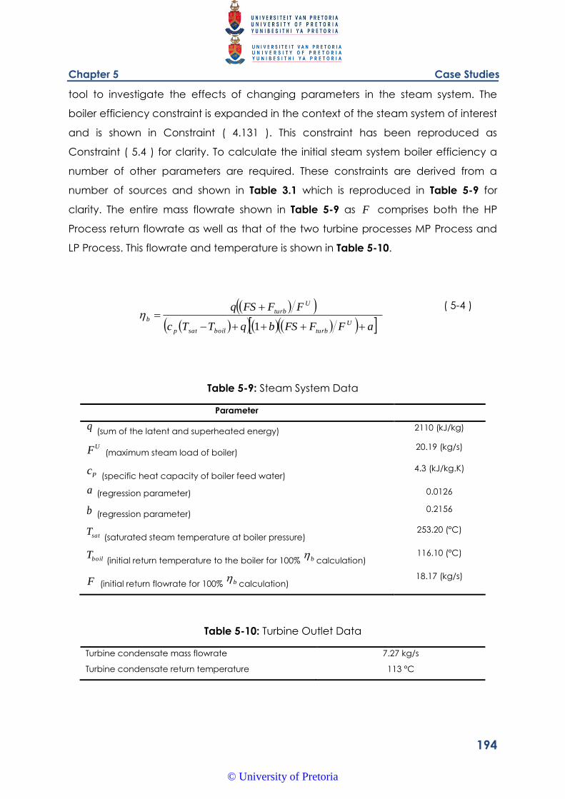
Chapter 5 Case Studies
194
tool to investigate the effects of changing parameters in the steam system. The
boiler efficiency constraint is expanded in the context of the steam system of interest
and is shown in Constraint ( 4.131 ). This constraint has been reproduced as
Constraint ( 5.4 ) for clarity. To calculate the initial steam system boiler efficiency a
number of other parameters are required. These constraints are derived from a
number of sources and shown in Table 3.1 which is reproduced in Table 5-9 for
clarity. The entire mass flowrate shown in Table 5-9 as F comprises both the HP
Process return flowrate as well as that of the two turbine processes MP Process and
LP Process. This flowrate and temperature is shown in Table 5-10.
aFFFSbqTTc
FFFSq
U
turbboilsatp
U
turb
b
1
( 5-4 )
Table 5-9: Steam System Data
Parameter
q (sum of the latent and superheated energy) 2110 (kJ/kg)
UF (maximum steam load of boiler) 20.19 (kg/s)
Pc (specific heat capacity of boiler feed water)
4.3 (kJ/kg.K)
a (regression parameter) 0.0126
b (regression parameter) 0.2156
satT (saturated steam temperature at boiler pressure)
253.20 (°C)
boilT (initial return temperature to the boiler for 100% b calculation)
116.10 (°C)
F (initial return flowrate for 100% b calculation) 18.17 (kg/s)
Table 5-10: Turbine Outlet Data
Turbine condensate mass flowrate 7.27 kg/s
Turbine condensate return temperature 113 °C
© University of Pretoria
Chapter 5 Case Studies
195
Thus using the initial steam system flowrate of 10.98 kg/s as well as the relevant
temperatures from Table 5-8 and parameters from Table 5-9 and Table 5-10 the
initial steam system boiler efficiency is calculated as 63.4%.
5.7.1. Solution from Price and Majozi (2010a)
As described in Section 3.4 and Section 4.8, by reducing the steam flowrate to a HEN
the boiler efficiency is negatively affected by both the reduction in the circulating
steam through the system as well as the associated decrease in the condensate
return temperature to the boiler. It was however found that increasing the
condensate return temperature would be able to maintain the boiler efficiency.
Price and Majozi (1010a) showed how after reducing the steam flowrate to a HEN
an additional pre heater can be added to the HEN in order to elevate the
condensate return temperature to such an extent that the boiler efficiency is
maintained.
The same steam system described in Section 5.1 was used as a case study for this
technique. The steam flowrate for the system was reduced from 10.98 kg/s to 7.68
kg/s. The original outlet temperature of the steam system was at the saturated
temperature of 225°C. By reducing the steam flowrate and utilising condensate to
heat a portion of the process streams the subsequent outlet temperature was
calculated as 46°C. Using the other parameters of the steam system which
remained unchanged, the boiler efficiency for the system was calculated as 59.8%,
a decrease of 3.6%.
By incorporating a dedicated pre heater into the HEN it was found that the boiler
efficiency could be effectively maintained at 63.4%. The steam flowrate required to
maintain the boiler efficiency at this level was found to be 8.76 kg/s. this is 13.9%
higher than the minimum steam flowrate of 7.68 kg/s but still a saving of 19.6% of the
original 10.98 kg/s. The process outlet temperature was found to be 60.4°C. This
resulted in a temperature of 84.2°C when combined with the turbine stream. The
duty of the additional heat exchanger was calculated as 2 256.4 kW. The return
stream to the boiler thus had a temperature of 117.0°C which was sufficient to
maintain the boiler efficiency for the reduced steam flowrate. The HEN arrangement
© University of Pretoria
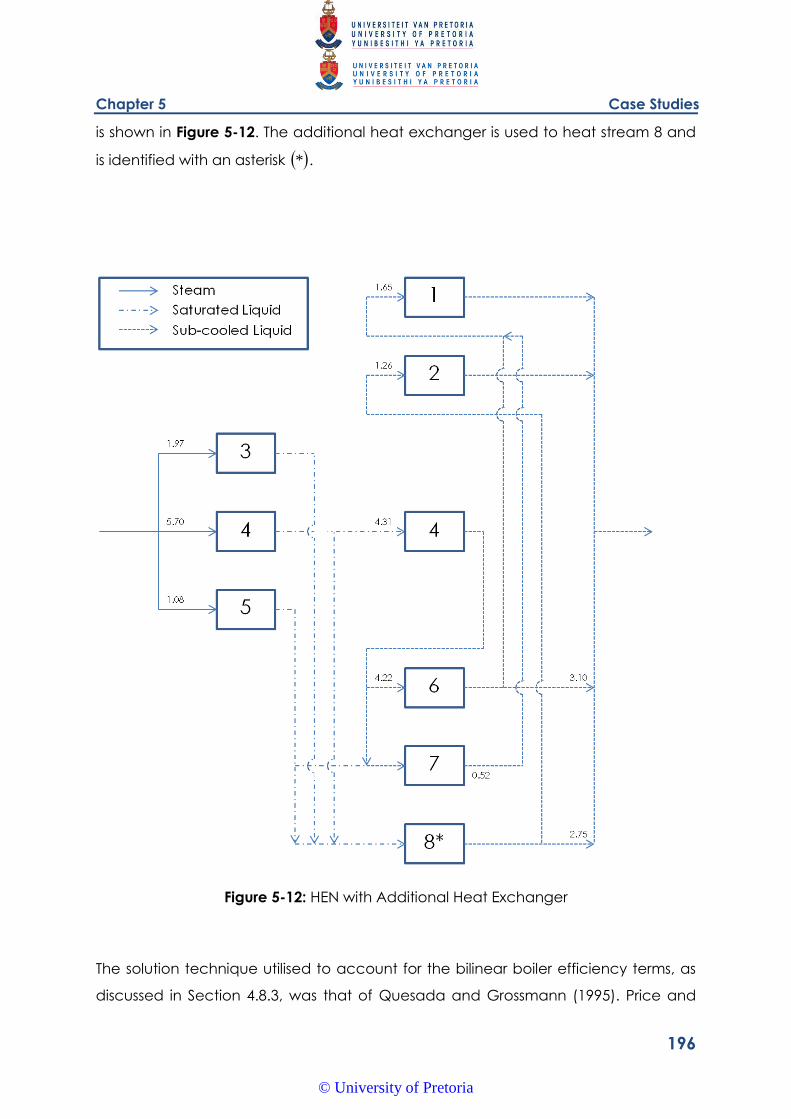
Chapter 5 Case Studies
196
is shown in Figure 5-12. The additional heat exchanger is used to heat stream 8 and
is identified with an asterisk * .
Figure 5-12: HEN with Additional Heat Exchanger
The solution technique utilised to account for the bilinear boiler efficiency terms, as
discussed in Section 4.8.3, was that of Quesada and Grossmann (1995). Price and
© University of Pretoria
Chapter 5 Case Studies
197
Majozi (2010a) found the solution to the MILP starting model to be 7.68 kg/s,
insinuating that the boiler efficiency could be maintained without the need for any
additional steam in the HEN. The solution of the exact MINLP revealed a steam
flowrate of 8.76 kg/s.
The pressure drop minimisation solution of Price and Majozi (2010c) was reworked to
remove singularities in the pressure drop constraints. This is not the case for the boiler
efficiency constraints and as such the solution of Price and Majozi (2010c) will be
maintained.
5.7.2. Degenerate Solution with Relaxation and Linearisation Formulation
This section describes the solution to the problem of maintaining boiler efficiency
with a dedicated pre heater while allowing for degenerate solutions within the
problem formulation.
The relaxation and linearisation formulation requires a large number of replacement
variables for those in the sensible energy constraint as was found for the pressure
drop minimisation case along with those found in calculating the boiler efficiency.
The relaxation and linearisation technique requires the solution of a linearised model
which becomes the starting point of the exact model. Unlike the solution of Price
and Majozi (2010a), the solution allowing for degenerate solutions will require the
terms in the sensible energy constraint to be treated in the same way as those of the
boiler efficiency constraints.
By incorporating the degenerate solutions to minimise the steam flowrate required to
maintain the boiler efficiency with an additional dedicated heat exchanger, the
solution to the MILP starting point problem was found to be 7.68 kg/s. This is identical
to that found by Price and Majozi (2010a). This suggests the boiler efficiency could
be maintained without the need to preheat the boiler return stream. Based on
observations and the boiler efficiency calculated after heat integration was applied
to the steam system this solution appears to be a large underestimate.
The solution to the exact MINLP was found to be 8.76 kg/s. This is identical to the
value found by Price and Majozi (2010a). The HEN arrangement however is quite
different and is shown in Figure 5-13.
© University of Pretoria
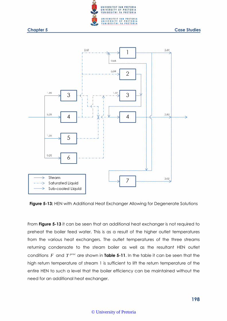
Chapter 5 Case Studies
198
Figure 5-13: HEN with Additional Heat Exchanger Allowing for Degenerate Solutions
From Figure 5-13 it can be seen that an additional heat exchanger is not required to
preheat the boiler feed water. This is as a result of the higher outlet temperatures
from the various heat exchangers. The outlet temperatures of the three streams
returning condensate to the steam boiler as well as the resultant HEN outlet
conditions F and procT are shown in Table 5-11. In the table it can be seen that the
high return temperature of stream 1 is sufficient to lift the return temperature of the
entire HEN to such a level that the boiler efficiency can be maintained without the
need for an additional heat exchanger.
© University of Pretoria
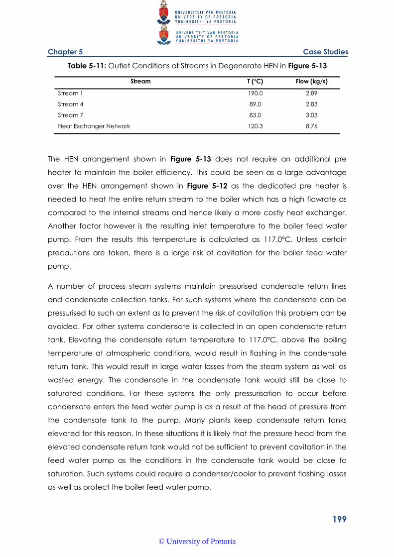
Chapter 5 Case Studies
199
Table 5-11: Outlet Conditions of Streams in Degenerate HEN in Figure 5-13
Stream T (°C) Flow (kg/s)
Stream 1 190.0 2.89
Stream 4 89.0 2.83
Stream 7 83.0 3.03
Heat Exchanger Network 120.3 8.76
The HEN arrangement shown in Figure 5-13 does not require an additional pre
heater to maintain the boiler efficiency. This could be seen as a large advantage
over the HEN arrangement shown in Figure 5-12 as the dedicated pre heater is
needed to heat the entire return stream to the boiler which has a high flowrate as
compared to the internal streams and hence likely a more costly heat exchanger.
Another factor however is the resulting inlet temperature to the boiler feed water
pump. From the results this temperature is calculated as 117.0°C. Unless certain
precautions are taken, there is a large risk of cavitation for the boiler feed water
pump.
A number of process steam systems maintain pressurised condensate return lines
and condensate collection tanks. For such systems where the condensate can be
pressurised to such an extent as to prevent the risk of cavitation this problem can be
avoided. For other systems condensate is collected in an open condensate return
tank. Elevating the condensate return temperature to 117.0°C, above the boiling
temperature at atmospheric conditions, would result in flashing in the condensate
return tank. This would result in large water losses from the steam system as well as
wasted energy. The condensate in the condensate tank would still be close to
saturated conditions. For these systems the only pressurisation to occur before
condensate enters the feed water pump is as a result of the head of pressure from
the condensate tank to the pump. Many plants keep condensate return tanks
elevated for this reason. In these situations it is likely that the pressure head from the
elevated condensate return tank would not be sufficient to prevent cavitation in the
feed water pump as the conditions in the condensate tank would be close to
saturation. Such systems could require a condenser/cooler to prevent flashing losses
as well as protect the boiler feed water pump.
© University of Pretoria
Chapter 5 Case Studies
200
An alternative solution would be to restrict the feed water pump inlet temperature in
the HEN design. This can be achieved by restricting collT in the formulation to a safe
pumping temperature sufficiently below the flashing temperature of condensate at
atmospheric conditions. An additional constraint was therefore added to the
formulation to restrict the inlet temperature to the boiler feed water pump. This is
shown in Constraint ( 5-5 ).
Ucollcoll TT , ( 5-5 )
In Constraint ( 5-5 ) the limiting collection temperature is denoted as UcollT , and can
be set at a level deemed safe for the boiler feed water pump. The lower the
temperature is set to, the larger the duty required for the additional pre heater is
likely to be. As an exercise the limit was set to 80°C.
The boiler efficiency was able to be maintained with a limiting collection
temperature. The steam flowrate was also able to be maintained at the level found
in Price and Majozi (2010a) of 8.76 kg/s. The HEN arrangement is shown in Figure
5-14.
© University of Pretoria
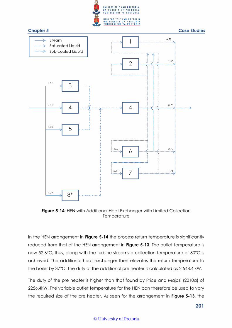
Chapter 5 Case Studies
201
Figure 5-14: HEN with Additional Heat Exchanger with Limited Collection
Temperature
In the HEN arrangement in Figure 5-14 the process return temperature is significantly
reduced from that of the HEN arrangement in Figure 5-13. The outlet temperature is
now 52.6°C, thus, along with the turbine streams a collection temperature of 80°C is
achieved. The additional heat exchanger then elevates the return temperature to
the boiler by 37°C. The duty of the additional pre heater is calculated as 2 548.4 kW.
The duty of the pre heater is higher than that found by Price and Majozi (2010a) of
2256.4kW. The variable outlet temperature for the HEN can therefore be used to vary
the required size of the pre heater. As seen for the arrangement in Figure 5-13, the
© University of Pretoria
Chapter 5 Case Studies
202
additional pre heater can be eliminated entirely with high return temperatures.
Restrictions on the condensate collection and pumping temperature should
however be taken into account for these formulations, which can now be achieved
with variable heat exchanger outlet temperatures. The design freedom provided by
incorporating degenerate solutions into the boiler efficiency framework can result in
savings in capital cost for new equipment as well as potentially allowing the system
to be further optimised for other network variables.
5.7.3. Degenerate Solution with Transformation and Convexification
Formulation
Initial Solution
This section describes the results attained for the problem of maintaining the boiler
efficiency of a steam system using a dedicated pre heater after the steam flowrate
to the system was minimised using methods of process integration.
As the steam flowrate to the system is unknown, no additional energy can be
allowed for by over estimations from the various transforms found in the formulation.
As such the same penalty functions as utilised in Constraint ( 4.122 ) were used in this
formulation. The positive slack variable described in Constraint ( 5-3 ) was included
to provide a feasible starting point where necessary.
The discretised solution process described in Section 4.6.5 is also problematic in the
boiler efficiency formulation due to the equality constraints relating the various pre
heater temperatures. This is due to the over estimation of the discretisations not
necessarily being equal to one another, unless the solution values appear at the
tangential point. This phenomena was observed with the pressure drop minimisation
formulation and was catered for with slack variables as shown in Constraint ( 5-3 ).
Slack variables were therefore also added to each of the temperature definition
constraints described by Constraints ( 4.136 ) to ( 4.138 ). The variables were then
added to the objective function which can be seen in Constraint ( 5-6 ).
© University of Pretoria
Chapter 5 Case Studies
203
slackneg
boil
slackpos
boil
slackneg
coll
slackpos
coll
slackneg
proc
slackpos
proc
i
slackneg
i
i
slackpos
i
TTTT
TTQLQLFSMinZ
( 5-6 )
Where is some penalty function constant. This constant is likely to take on a high
value as additional energy will distort the solution greatly.
As discussed in Section 5.4.1, a number of modelling variables play a part in the
solution process. Using the modelling experience from Section 5.4.1 a number of
these modelling variables were attempted but no feasible solution was found.
Equality constraints were also simplified to two inequality constraints as is advised in
Pörn et al. (2008). This formulation did not result in any feasible solutions.
Further Modelling
The transformation and convexification formulation presented with linearised
functions for the convexification variables is complex to solve when ET and PT
transforms appear in many constraints. As the linearisations are not necessarily
equivalent, the constraints cannot always be represented as equality constraints but
rather as inequality constraints to allow for variations in the degree of linearisation.
This is particularly prevalent in the boiler efficiency problem as many of the bilinear
terms appear in equality constraints. These constraints can be represented with a
combination of inequality constraints which was completed for the formulation.
Slack variables were provided to the formulation in an attempt to counter this
phenomenon with limited success.
Linearisations allow the entire problem to be convexified, however, as described in
Pörn et al. (2008), by transforming the complex bilinear terms into convex terms and
effectively transferring the nonconvexity to a single term in a constraint this can
simplify the problem. This approach was attempted for the boiler efficiency problem.
All transformation variables were formulated without discretisations. The resultant
MINLP is nonconvex due to the natural logarithm and square functions in the
formulation for the ET and PT respectively.
© University of Pretoria
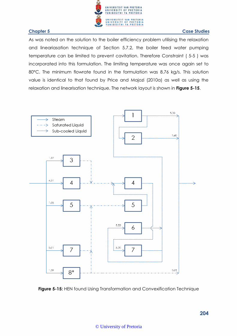
Chapter 5 Case Studies
204
As was noted on the solution to the boiler efficiency problem utilising the relaxation
and lineariasation technique of Section 5.7.2, the boiler feed water pumping
temperature can be limited to prevent cavitation. Therefore Constraint ( 5-5 ) was
incorporated into this formulation. The limiting temperature was once again set to
80°C. The minimum flowrate found in the formulation was 8.76 kg/s. This solution
value is identical to that found by Price and Majozi (2010a) as well as using the
relaxation and linearisation technique. The network layout is shown in Figure 5-15.
Figure 5-15: HEN found Using Transformation and Convexification Technique
© University of Pretoria
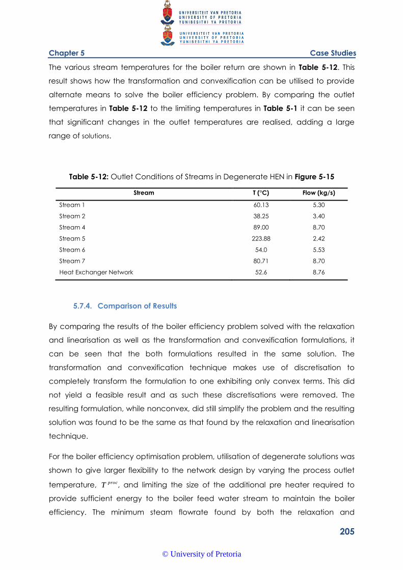
Chapter 5 Case Studies
205
The various stream temperatures for the boiler return are shown in Table 5-12. This
result shows how the transformation and convexification can be utilised to provide
alternate means to solve the boiler efficiency problem. By comparing the outlet
temperatures in Table 5-12 to the limiting temperatures in Table 5-1 it can be seen
that significant changes in the outlet temperatures are realised, adding a large
range of solutions.
Table 5-12: Outlet Conditions of Streams in Degenerate HEN in Figure 5-15
Stream T (°C) Flow (kg/s)
Stream 1 60.13 5.30
Stream 2 38.25 3.40
Stream 4 89.00 8.70
Stream 5 223.88 2.42
Stream 6 54.0 5.53
Stream 7 80.71 8.70
Heat Exchanger Network 52.6 8.76
5.7.4. Comparison of Results
By comparing the results of the boiler efficiency problem solved with the relaxation
and linearisation as well as the transformation and convexification formulations, it
can be seen that the both formulations resulted in the same solution. The
transformation and convexification technique makes use of discretisation to
completely transform the formulation to one exhibiting only convex terms. This did
not yield a feasible result and as such these discretisations were removed. The
resulting formulation, while nonconvex, did still simplify the problem and the resulting
solution was found to be the same as that found by the relaxation and linearisation
technique.
For the boiler efficiency optimisation problem, utilisation of degenerate solutions was
shown to give larger flexibility to the network design by varying the process outlet
temperature, procT , and limiting the size of the additional pre heater required to
provide sufficient energy to the boiler feed water stream to maintain the boiler
efficiency. The minimum steam flowrate found by both the relaxation and
© University of Pretoria
Chapter 5 Case Studies
206
linearisation technique as well as the transformation and convexification technique
was found to be the same as those found by Price and Majozi (2010a). The network
structures for these solutions all differ significantly, suggesting further optimisation
potential for another network variable such as heat exchange area or pressure
drop.
No feasible solution was found using the discretised transformation and
convexification formulation. It is believed that complexities arise when utilising the
discretised form of the formulation when working with branch and bound type
MINLP solvers due to limited solution space. This result mimics the experience from
the pressure drop minimisation problem.
5.8. References
Coetzee, W.A. and Majozi, T. (2008) Steam System Network Design Using Process
Integration, Industrial Engineering Chemistry Research 2008, 47, 4405-4413.
Kocis, G. R. and Grossmann, I. E. (1989) A Modelling and Decomposition Strategy for
MINLP Optimization of Process Flowsheets, Computers and Chemical Engineering ,
13 (7), 797-819.
Pörn, R., Bjork, K., and Westerlund, T. (2008) Global solution of optimization problems
with signomial parts. Discrete Optimization 5 , 108-120.
Price, T. and Majozi, T. (2010a) On Synthesis and Optimization of Steam System
Networks. 1. Sustained Boiler Efficiency. Industrial Engineering Chemistry Research 49
, 9143–9153.
Price, T. and Majozi, T. (2010c) On Synthesis and Optimization of Steam System
Networks. 3. Pressure Drop Consideration. Industrial Engineering Chemistry Research
49 , 9165–9174.
Quesada, I. and Grossmann, I. E. (1995) Global optimisation of bilinear process
networks with multi component flows, Computers and Chemical Engineering 19, No
12, pages 1219-1242.
© University of Pretoria
Chapter 5 Case Studies
207
Savelski, M. J. and Bagajewicz, M. J. (2000) On the optimality conditions of water
utilization systems in process plants with single contaminants, Chemical Engineering
Science 55, pages 5035-5048.
Sinnot, R. K. (2005) Chemical engineering design, Vol 6, Elsevier Butterworth
Heinemann, New York.
© University of Pretoria
Chapter 6 Conclusions and Discussion
208
6. Conclusions and Discussion
This chapter summarises the findings of this work and discusses areas of further
application and potential research.
6.1. Conclusions
Minimum heating and cooling utilities can be determined for process HENs. A
technique used to find the heating or cooling utility flowrate is a condition of
network optimality where the limiting temperatures of the heat exchangers are set
to their bounds. This approach typically results in a linear problem which can be
solved to global optimality. The minimum flowrate can be achieved with an infinite
number of network arrangements therefore additional system variables can be
optimised while still maintaining the minimum steam flowrate.
Once a minimum utility flowrate is found the conditions of network optimality can be
relaxed in order to further optimise additional system variables. This is due to the
solution space for the system being enlarged by allowing the limiting temperatures
of utility streams leaving heat exchangers to vary.
By allowing the outlet temperatures to vary bilinear terms are created in the energy
constraints in the formulation. Bilinear terms are nonlinear and nonconvex and
therefore present difficulties to conventional optimisation solvers.
This work presents the optimisation of two system variables, namely heat exchanger
network pressure drop for heating systems as well as boiler efficiency. Two methods
are proposed to cater for the bilinear terms created by relaxing the conditions of
network optimality. The results from case studies were compared with previous work
in order to determine the effectiveness of the methods.
6.1.1. Pressure Drop Comparison
The minimum HEN pressure drop presented by Price and Majozi (2010c) was
achieved by relaxing the minimum steam flowrate. This is due to singularities formed
© University of Pretoria
Chapter 6 Conclusions and Discussion
209
when flow variables take zero values. The model was resolved using translations to
shift the flow variables away from zero. This allowed the minimum pressure drop to
be found while still retaining the exact minimum steam flowrate. The model was
solved successfully as an MINLP problem.
The minimum HEN pressure drop for this system was found to be 364.430 kPa. This
result shows how translations can be used effectively to overcome singularities. An
effective means to find a network that exhibits the minimum pressure drop while still
achieving the minimum steam flowrate has been created successfully. A second
case study was used to determine the rigorousness of this technique and a minimum
system pressure drop of 164.16 kPa was achieved.
By allowing degenerate solutions to the HEN pressure drop minimisation problem the
size of the solution space is enlarged. This comes at the expense of nonlinear,
nonconvex bilinear terms being added to the formulation. These bilinear terms can
be reformulated using the relaxation and linearisation formulation. Using this
technique a better pressure drop for the system was found using two case studies.
The first case study resulted in a minimum pressure drop of 360.46 kPa, an
improvement of 1.1%. This result shows how degenerate solutions can be used to
improve the solutions to nonlinear network optimisation problems. A solution of the
second case study was found to be 151.95 kPa. This is an improvement of 7.1% from
the fixed heat exchanger outlet temperature solution.
The same problem was attempted using the transformation and convexification
technique to create a convex problem which is much more easily solvable with
conventional MINLP solvers. This technique was not found to be as successful in
finding a minimum pressure drop. This is understood to be due to the nature of the
discretisation process which accompanies the transformation step of the
formulation. The discretisation is accomplished using binary variables which limit the
NLP sub problem solution space when using branch and bound type MINLP solvers.
The solution was found not to converge to a point where the discretisation did not
unduly benefit the formulation, skewing the minimum pressure drop results. The use of
this technique to address degenerate solutions and their benefits over formulations
utilising only the conditions of network optimality was tested by comparing the
solution of the two problems with the same degree of relaxation provided by the
© University of Pretoria
Chapter 6 Conclusions and Discussion
210
discretisation of the transformation and convexification technique. The pressure
drop found by effectively adding the same degree of sensible energy to the fixed
outlet temperature formulation was 208.15 kPa. The solution utilising degenerate
solutions was found to be 209.20 kPa.
By a comparison of the results the relaxation and linearisation technique allowed a
feasible solution to be found and a better minimum HEN pressure drop was
achieved in two case studies. The discretised transformation and convexification
technique was unable to find a feasible solution to the network pressure drop
minimisation problem. Therefore it is concluded that the relaxation and linearization
technique was the favoured of the two investigated in this work.
6.1.2. Boiler Efficiency Comparison
The steam flowrate to a HEN can be minimised by utilising saturated and sub cooled
condensate as a source of energy. The resulting reduction in steam flowrate and
condensate return temperature negatively affects the efficiency of the steam boiler.
The boiler efficiency can however be maintained by incorporating an additional
dedicated heat exchanger into the HEN to pre heat the boiler feed water return.
This was accomplished by Price and Majozi (2010a).
The minimum steam flowrate from the system was slightly compromised by this
alteration as additional energy was required to pre heat the boiler feed water. This
minimum flowrate was found to be 8.76 kg/s with an additional pre heater duty of
2256.4kW.
As described in Section 6.1.1, incorporating degenerate solutions enlarges the size of
the solution space for the HEN arrangement. The variables required to calculate the
boiler efficiency can therefore vary more, allowing for more flexible solutions. The
minimum steam flowrate found using the relaxation and linearisation technique was
8.76 kg/s which is identical to that found by Price and Majozi (2010a). The required
duty of the pre heater for the two cases was however different, with the degenerate
solution case being able to vary depending on the outlet temperatures of the
individual heat exchangers. With no limitation to the HEN outlet temperature the
need for an additional pre heater was removed due to high return temperatures.
This could potentially cause cavitation in the boiler feed water pump and therefore
© University of Pretoria
Chapter 6 Conclusions and Discussion
211
the pumping temperature was limited. The resulting duty was found to be 2548.4 kW.
In general, the duty of the pre heater can be varied by changing the outlet
temperature of the HEN which was not previously feasible with limited heat
exchanger outlet temperatures.
The transformation and convexification technique was utilised with discretised
transformation variables as described by Pörn et al. (2008). This formulation did not
result in a feasible solution. The undiscretised transformation and convexification
formulation did however result in a minimum flowrate of 8.76 kg/s, once again
identical to that of Price and Majozi (2010a). Once again the HEN arrangement was
found to be more flexible and the pre heater duty could be varied by limiting the
HEN outlet temperature. By not discretising the transformation variables in the
transformation and convexification formulation the resulting MINLP is nonconvex and
therefore the global optimality of the solution cannot be guaranteed.
The relaxation and linearisation as well as the transformation and convexification
techniques were found to be successful at dealing with the bilinear terms arising
from incorporating degenerate solutions in the formulation. The results using the two
techniques were identical in terms of minimum steam flowrate, however the
transformation and convexification technique could not guarantee global
optimality due to the undiscretised and hence nonconvex formulation providing the
only feasible solution.
6.2. Discussion
This work shows that degenerate solutions should be investigated to optimise
network variables once a minimum utility flowrate has been found. For network
pressure drop it is suggested that the minimum network flowrate is found, then the
minimum pressure drop is found using conditions of network optimality and then
degenerate solutions are investigated in an attempt to further minimise the network
pressure drop. Similarly, for boiler efficiency optimisation, a minimum steam flowrate
for the HEN should be found using established techniques. The boiler efficiency for
the system can then be maintained for retrofit steam systems using sources of heat
within the steam systems or a dedicated additional heat exchanger. By
© University of Pretoria
Chapter 6 Conclusions and Discussion
212
incorporating degenerate solutions, the steam system is allowed additional degrees
of freedom to accommodate more design constraints, such as boiler feed water
pumping temperature. The size and duty of additional equipment can be optimised
due to the variable HEN outlet temperature brought about by the allowance for
degenerate solutions.
It must be noted that improvements in HEN pressure drop and the series heat
exchanger connections discussed in this work will result in higher HEN
interconnectivity which could make general operability as well as abnormal
operations such as startup or shutdown more difficult. When incorporating any
aspects of process integration into design, aspects such as operability and process
control should also be considered. By formalising better techniques for process
integration, a more effective iterative approach which gives consideration to
aspects such as control are more feasible and less time consuming.
The techniques utilised in this work are not necessarily the only techniques that are
effective at dealing with bilinear terms. Further, other solvers may also be more
effective at finding a more optimal solution.
From the outset of this research and that of preceding work stochastic type
optimisation algorithms such as Genetic Algorithms (GA) were not as effective at
solving nonconvex MINLP problems. Therefore the focus of this and preceding work
was on the operation of deterministic algorithms and how these behave when
applied to the formulations presented. Subsequently large advances in the
robustness and effectiveness of stochastic algorithms have resulted in them
becoming competitive as compared to deterministic algorithms. Future work could
include the use of stochastic algorithms to explore the potential benefits of including
degenerate solutions in exchange network optimisation.
Future work in this field could also include the update of the transformation and
convexification technique which may be found to yield a more optimal HEN
pressure drop. Boiler efficiency optimisation using the discretised transformation and
convexification technique should be further explored as this technique was found to
not result in a feasible solution. The undiscretised formulation was successful at
© University of Pretoria
Chapter 6 Conclusions and Discussion
213
finding a solution however due to the nonconvex nature of the constraints the
global optimality of the solution cannot be guaranteed.
The relaxation and linearisation technique was found to be effective at achieving
an improved network pressure drop with degenerate solutions.
The transformation and convexification technique has been shown to be effective
at aiding the solutions of complex nonconvex problems however the application
with branch and bound type MINLP solvers was not as effective as the relaxation
and linearisation technique. The use of tangential piecewise linear approximations
for the purposes of discretising certain variables is effective at ensuring a variable
can take the value above or below a particular limit if necessary. These techniques
have the potential to yield better solutions to network optimisation problems where
nonlinear constraints are present.
6.3. References
Pörn, R., Bjork, K., and Westerlund, T. (2008) Global solution of optimization problems
with signomial parts. Discrete Optimization 5 , 108-120.
Price, T. and Majozi, T. (2010) On Synthesis and Optimization of Steam System
Networks. 1. Sustained Boiler Efficiency. Industrial Engineering Chemistry Research 49
, 9143–9153.
Price, T. and Majozi, T. (2010) On Synthesis and Optimization of Steam System
Networks. 3. Pressure Drop Consideration. Industrial Engineering Chemistry Research
49 , 9165–9174.
© University of Pretoria
Chapter 6 Conclusions and Discussion
214
Appendix A.
This section of the Appendix is intended to show how the unknown terms relating to
the heat exchanger and piping pressure drop correlations have been derived for
the pressure drop mathematical model.
A.1. Heat Exchanger Guidelines
Constraints ( 3-2 ) and ( 3-3 ) contain the following heat exchanger design based
variables; heat transfer area A , the number of tube passes tpn , the number of tubes
tN , the inside tube diameter id and the outside tube diameter od .
For the various heat exchangers in the relevant case study the heat transfer area is
determined using the general equation for heat transfer defined in Sinnot (2005),
shown in Constraint (A.1)
mTUAQ ( 6-1 )
In Constraint ( 6-1 ) Q is the relevant duty for the stream to be heated, U is the overall
heat transfer coefficient, A is the heat transfer area and mT is the log mean
temperature difference. The stream duty is known for the case studies. An
approximate overall heat transfer coefficient is taken from Sinnot (2005). This value is
1000 W/m2.K for the condensers and 800 W/m2.K for the condensate heat
exchangers. The mT for condensers is determined using Constraint ( 6-2 ) as defined
by Sinnot (2005).
© University of Pretoria
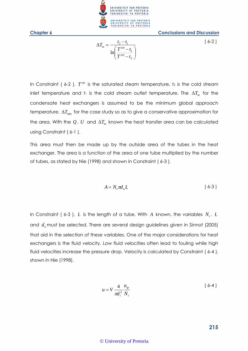
Chapter 6 Conclusions and Discussion
215
2
1
12
lntT
tT
ttT
sat
satm ( 6-2 )
In Constraint ( 6-2 ), satT is the saturated steam temperature, t2 is the cold stream
inlet temperature and t1 is the cold stream outlet temperature. The mT for the
condensate heat exchangers is assumed to be the minimum global approach
temperature, minT for the case study so as to give a conservative approximation for
the area. With the Q , U and mT known the heat transfer area can be calculated
using Constraint ( 6-1 ).
This area must then be made up by the outside area of the tubes in the heat
exchanger. The area is a function of the area of one tube multiplied by the number
of tubes, as stated by Nie (1998) and shown in Constraint ( 6-3 ).
LdNA ot ( 6-3 )
In Constraint ( 6-3 ), L is the length of a tube. With A known, the variables tN , L
and od must be selected. There are several design guidelines given in Sinnot (2005)
that aid in the selection of these variables. One of the major considerations for heat
exchangers is the fluid velocity. Low fluid velocities often lead to fouling while high
fluid velocities increase the pressure drop. Velocity is calculated by Constraint ( 6-4 ),
shown in Nie (1998).
t
tp
iN
n
dVu
2
4
( 6-4 )
© University of Pretoria
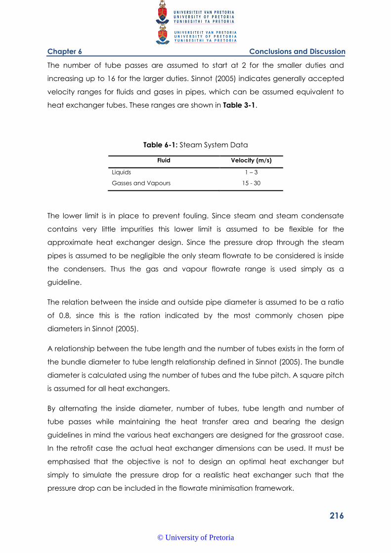
Chapter 6 Conclusions and Discussion
216
The number of tube passes are assumed to start at 2 for the smaller duties and
increasing up to 16 for the larger duties. Sinnot (2005) indicates generally accepted
velocity ranges for fluids and gases in pipes, which can be assumed equivalent to
heat exchanger tubes. These ranges are shown in Table 3-1.
Table 6-1: Steam System Data
Fluid Velocity (m/s)
Liquids 1 – 3
Gasses and Vapours 15 - 30
The lower limit is in place to prevent fouling. Since steam and steam condensate
contains very little impurities this lower limit is assumed to be flexible for the
approximate heat exchanger design. Since the pressure drop through the steam
pipes is assumed to be negligible the only steam flowrate to be considered is inside
the condensers. Thus the gas and vapour flowrate range is used simply as a
guideline.
The relation between the inside and outside pipe diameter is assumed to be a ratio
of 0.8, since this is the ration indicated by the most commonly chosen pipe
diameters in Sinnot (2005).
A relationship between the tube length and the number of tubes exists in the form of
the bundle diameter to tube length relationship defined in Sinnot (2005). The bundle
diameter is calculated using the number of tubes and the tube pitch. A square pitch
is assumed for all heat exchangers.
By alternating the inside diameter, number of tubes, tube length and number of
tube passes while maintaining the heat transfer area and bearing the design
guidelines in mind the various heat exchangers are designed for the grassroot case.
In the retrofit case the actual heat exchanger dimensions can be used. It must be
emphasised that the objective is not to design an optimal heat exchanger but
simply to simulate the pressure drop for a realistic heat exchanger such that the
pressure drop can be included in the flowrate minimisation framework.
© University of Pretoria
Chapter 6 Conclusions and Discussion
217
A.2. Piping Guidelines
Constraint ( 3.5 ) is a fairly simple piping pressure drop estimation. Since an
economic design guideline of Peters and Timmerhaus (1991) has already been used
to derive the constraint the only choice left is the pipe length. In the model the
various types of pipe length are varied. The recycle and reuse pipes are assumed to
be longer than the pipes joining the heat exchangers to the central condensate
return hub.
A.3. References
Nie, X. R. (1998) Heat exchanger network retrofit considering pressure drop and heat
transfer enhancement, Ph.D. Thesis, UMIST, Manchester.
Peters, M. S. and Timmerhaus, K. D. (1991) Plant design and economics for chemical
engineers, 4th Edition, Mcgraw-Hill, New York.
Sinnot, R. K. (2005) Chemical engineering design, Vol 6, Elsevier Butterworth
Heinemann, New York.
© University of Pretoria
Chapter 6 Conclusions and Discussion
218
Appendix B.
This section of the Appendix includes a description of the linearisation techniques
used in this dissertation. Two linearisations are described. The first is applicable for the
bilinear product of two continuous variables and the technique is illustrated by
Quesada and Grossmann (1995). The second is applicable for the bilinear product
of a continuous variable and a binary variable and this method is explained by
Glover (1975).
B.1. Relaxation Linearisation Technique Described by Quesada and
Grossmann (1995)
Let
xy , where x and y are both continuous variables in the formulation. In the
case of this dissertation x is a temperature and y is a flowrate.
with each variable displaying the following bounds
UL XxX ( 6-5 )
UL YyY ( 6-6 )
each of the bounds expressed as individual equations
0 LXx ( 6-7 )
© University of Pretoria
Chapter 6 Conclusions and Discussion
219
0 xX U ( 6-8 )
0 LYy ( 6-9 )
0 yY U ( 6-10 )
performing the following multiplications
ULLU YXyXxYxyCC 63 ( 6-11 )
LUUL YXyXxYxyCC 54 ( 6-12 )
LLLL YXyXxYxyCC 53 ( 6-13 )
UUUU YXyXxYxyCC 64 ( 6-14 )
This linearisation technique is not exact. It does however create a convex solution
space where the linearised model is solved. This solution is then used as a starting
point for the exact, nonlinear model. To implement this technique Constraints ( 6-11 )
to ( 6-14 ) are included in the formulation for the linear model and all the bilinear
terms are replaced with Γ. If the solution to the nonlinear model equals that of the
linear model it can be concluded that a globally optimal solution exists. If the
solutions differ then it can be concluded that the solution for the exact, nonlinear
model is feasible but not globally optimal.
© University of Pretoria
Chapter 6 Conclusions and Discussion
220
B.2. Glover (1975) Transformation
Let
xy , where x and 1,0y
the following restrictions also hold
00 when 0y ( 6-15 )
xx when 1y ( 6-16 )
the following bounds are applicable
UL MM ( 6-17 )
then the following constraints on hold
yMyM UL ( 6-18 )
yMxyMx LU 11 ( 6-19 )
Constraints ( 6-18 ) and ( 6-1 ) are then added to the formulation and the bilinear
term xy is replaced with the new linearisation variable . This linearisation
© University of Pretoria
Chapter 6 Conclusions and Discussion
221
technique is exact and will therefore result in a globally optimal solution if all of the
other constraints in the formulation are linear.
B.3. References
Glover, F. (1975) Improved linear integer programming formulation of nonlinear
problems, Management Science, Pages 455-460.
Quesada, I. and Grossmann, I. E. (1995) Global optimisation of bilinear process
networks with multi component flows, Computers and Chemical Engineering 19, No
12, pages 1219-1242.
© University of Pretoria


![Methanol Steam Reforming Performance Optimisation of ... · were used as optimisation objects by utilising the coupling method and artificial neural networks [23]. Although some research](https://img.pdfslide.us/doc/110x75/5f1acffd2be672440c330099/methanol-steam-reforming-performance-optimisation-of-were-used-as-optimisation.jpg)