Optimal Design and Operation of Massively Dense Wireless Networks(or How to Study 21st Century Problems with 19th Century Math)

Stavros Toumpis, University of Cyprus

Inter-perf 2006, Pisa, Oct. 14 2006

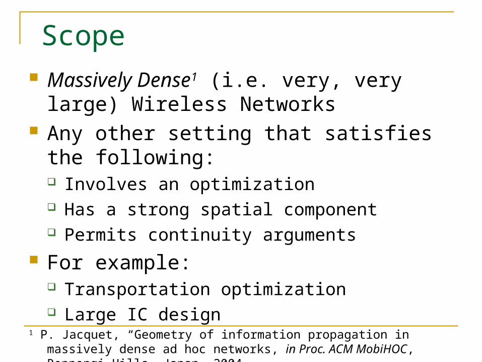
Scope Massively Dense1 (i.e. very, very large)

Wireless Networks Any other setting that satisfies the following:

Involves an optimization Has a strong spatial component Permits continuity arguments

For example: Transportation optimization Large IC design

1 P. Jacquet, “Geometry of information propagation in massively dense ad hoc networks, in Proc. ACM MobiHOC, Roppongi Hills, Japan, 2004.

Appetizer

05.01030

1),( 24 xyx

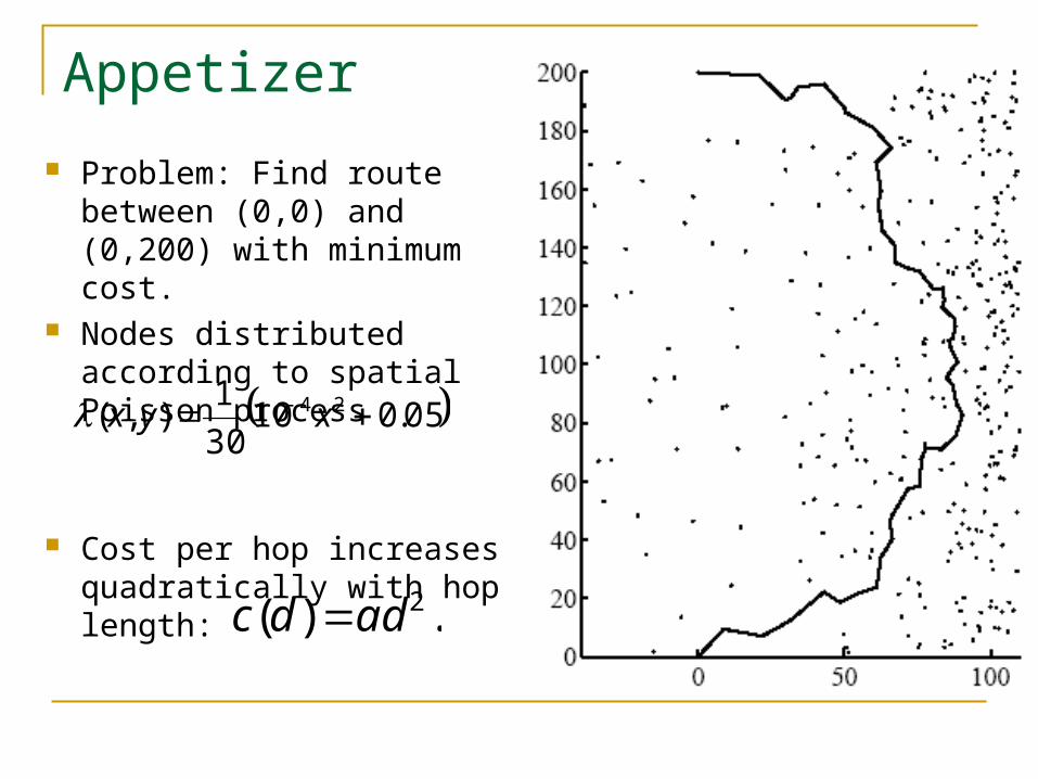
Problem: Find route between (0,0) and (0,200) with minimum cost.

Nodes distributed according to spatial Poisson process

Cost per hop increases quadratically with hop length:

.)( 2addc

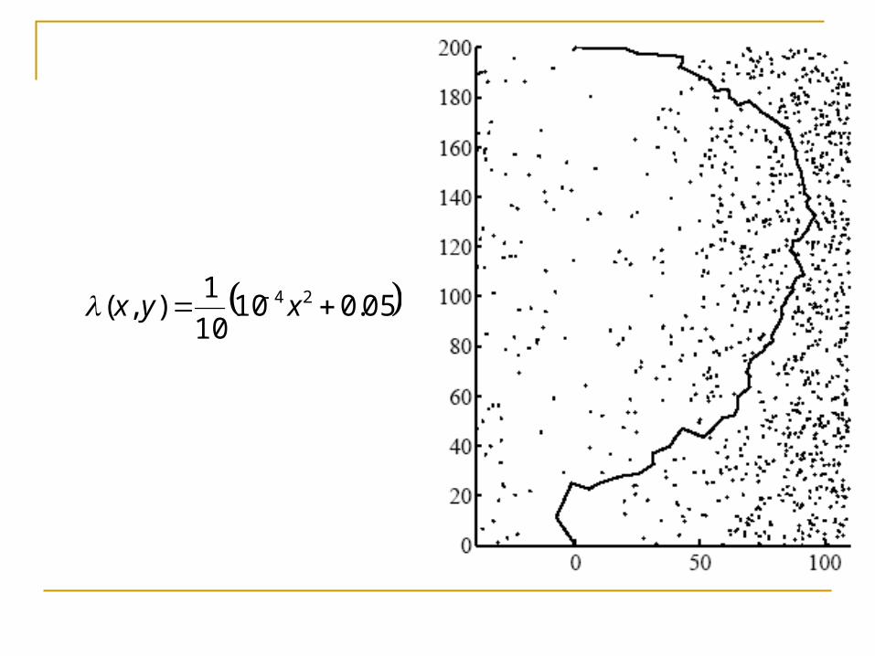
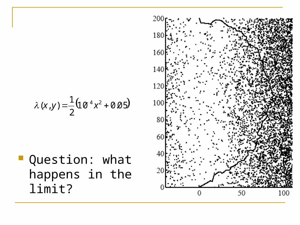
05.01010

1),( 24 xyx

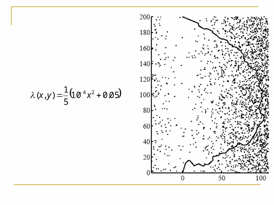
05.0105

1),( 24 xyx

05.0102

1),( 24 xyx

Question: what happens in the limit?

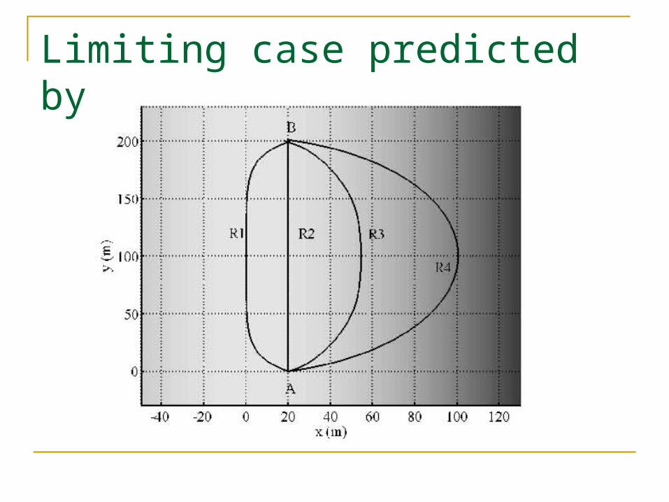
Limiting case predicted by Optics

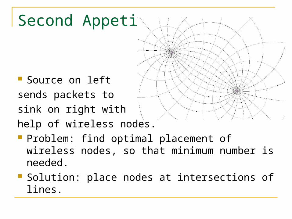
Second Appetizer

Source on left

sends packets to

sink on right with

help of wireless nodes. Problem: find optimal placement of wireless

nodes, so that minimum number is needed. Solution: place nodes at intersections of lines.

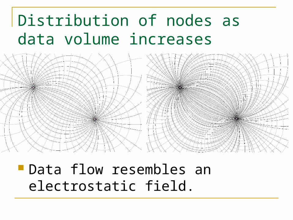
Distribution of nodes as data volume increases

Data flow resembles an electrostatic field.

Central Idea of this Talk: Macroscopic View Many problems in wireless networking (and

elsewhere) are way too complicated to be solved without proper abstractions.

Standard approach is based on microscopic quantities: individual node placement, individual link properties, etc.

We can take a novel macroscopic approach, using macroscopic quantities: node density, data creation density, etc.

Central Idea (cont’) Macroscopic quantities are connected with

each other through ‘constitutive laws’. Microscopic considerations enter only through

these laws. Approach opens gateway to new (or old,

depending on how you look at it) Math: Calculus of Variations, Partial Differential

Equations, Optics, Electrostatics, etc. Results are not as detailed as with standard

approach, but detailed enough to remain useful.

Contents

Introduction “Packetostatics” “Packetoptics” Cooperative Transmissions Energy Efficient Routing Load Balancing

2. “Packetostatics”

G. Gupta, IIT New Delhi

L. Tassiulas, University of Thessaly

S. Toumpis, University of Cyprus

Setting

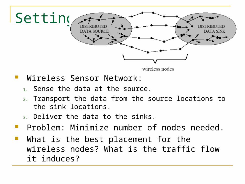
Wireless Sensor Network:1. Sense the data at the source.

2. Transport the data from the source locations to the sink locations.

3. Deliver the data to the sinks. Problem: Minimize number of nodes needed. What is the best placement for the wireless nodes?

What is the traffic flow it induces?

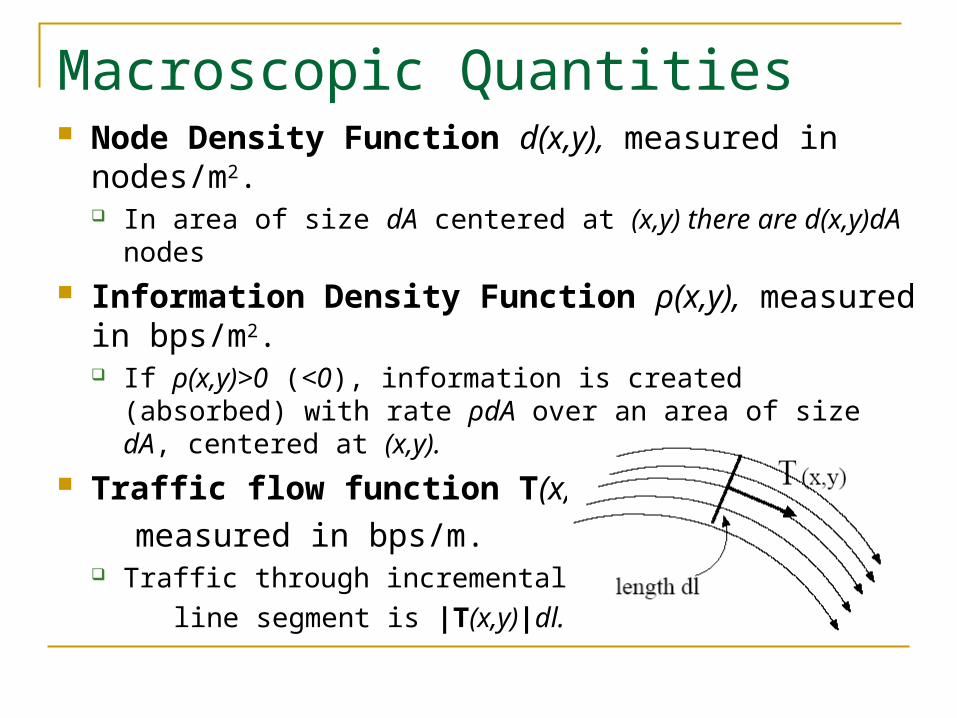
Macroscopic Quantities Node Density Function d(x,y), measured in

nodes/m2. In area of size dA centered at (x,y) there are d(x,y)dA nodes

Information Density Function ρ(x,y), measured in bps/m2. If ρ(x,y)>0 (<0), information is created (absorbed) with rate

ρdA over an area of size dA, centered at (x,y). Traffic flow function T(x,y),

measured in bps/m. Traffic through incremental

line segment is |T(x,y)|dl.

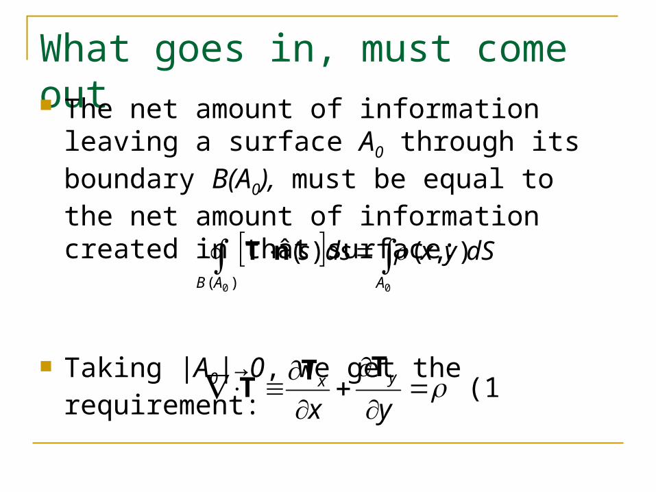
What goes in, must come out The net amount of information leaving a

surface A0 through its boundary B(A0), must be equal to the net amount of information created in that surface:

Taking |A0|→0, we get the requirement:

)( 0 0

),()(ˆAB A

dSyxdss nT

(1)

yxyxTT

T

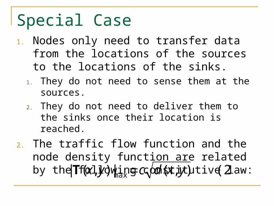
Special Case1. Nodes only need to transfer data from the

locations of the sources to the locations of the sinks.

1. They do not need to sense them at the sources.

2. They do not need to deliver them to the sinks once their location is reached.

2. The traffic flow function and the node density function are related by the following constitutive law:

(2) ),(|),(| max yxdcyx T

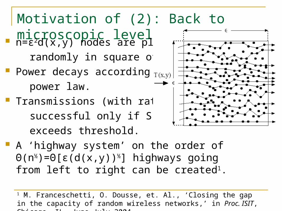
Motivation of (2): Back to microscopic level n=ε2d(x,y) nodes are placed

randomly in square of side ε. Power decays according to

power law. Transmissions (with rate W),

successful only if SINR

exceeds threshold. A ‘highway system’ on the order of

Θ(n½)=Θ[ε(d(x,y))½] highways going from left to right can be created1.

1 M. Franceschetti, O. Dousse, et. Al., ‘Closing the gap in the capacity of random wireless networks,’ in Proc. ISIT, Chicago, IL, June-July 2004

Traffic must be irrotational

We must minimize the number of nodes

If (2) is satisfied, then the traffic must be irrotational:

Easy proof by contradiction.

.),( dAyxdN

.0

yxxy TT

T

‘Packetostatics’ The traffic flow T and information density ρ must

satisfy:

In uniform dielectrics (e.g., free space), the electric field E and the charge density ρ are uniquely determined by:

Therefore, the optimal traffic distribution is the same with the electric field when we substitute the sources and sinks with positive and negative charges!

.0 , TT

.0 , EE

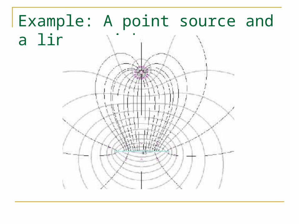
Example: A point source and a linear sink

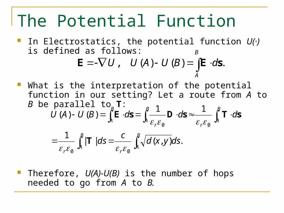
The Potential Function In Electrostatics, the potential function U(·) is defined as

follows:

What is the interpretation of the potential function in our setting? Let a route from A to B be parallel to T:

Therefore, U(A)-U(B) is the number of hops needed to go from A to B.

.)()( , B

A

dBUAUU sEE

.),(||1

11)()(

00

00

B

Ar

B

Ar

B

Ar

B

A

B

Ar

dsyxdc

ds

dddBUAU

T

sTsDsE

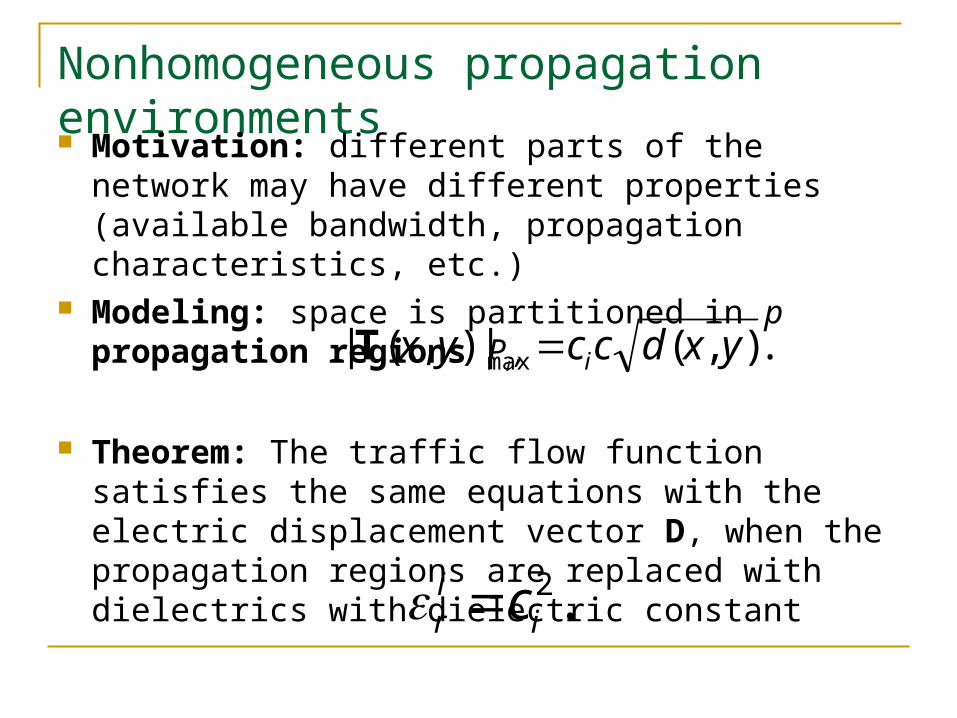
Nonhomogeneous propagation environments Motivation: different parts of the network may

have different properties (available bandwidth, propagation characteristics, etc.)

Modeling: space is partitioned in p propagation regions Pi ,

Theorem: The traffic flow function satisfies the same equations with the electric displacement vector D, when the propagation regions are replaced with dielectrics with dielectric constant

.),(|),(| max yxdccyx iT

.2i

ir c

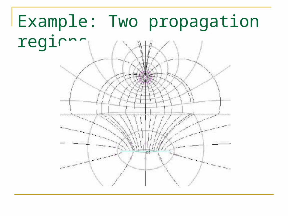
Example: Two propagation regions

Thomson’s Theorem Consider a number of perfect conductors Ci, each

infused with some electric charge Qi. Conductors are placed within a region of space that may contain dielectrics.

Basic Question: How do the charges distribute themselves on the conductors?

Thomson’s Theorem: The charges are distributed so as to minimize the electrostatic energy of the setting:

.),(22

22

dAyxddAcc

dAdAEi

ir

TDDE

Sources and sinks with freedom in placement Motivation: In some cases, we have some

freedom on the placement of the sources/sinks. Modeling: Consider t traffic regions Ti, i=1,…,t

each associated with an information rate Qi.

Question: What is the optimal deployment of Qi in Ti?

Answer: By Thomson’s theorem, the optimal deployment of Qi makes the traffic flow look like the electrostatic field when the Qi are charges and Ti are perfect conductors.

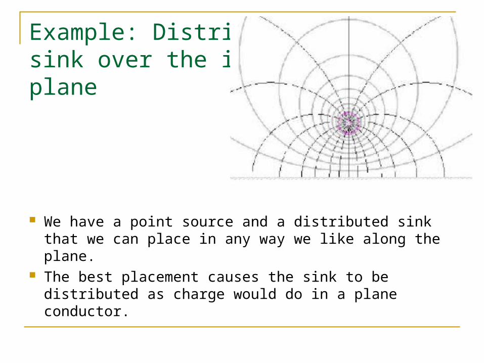
Example: Distributed sink over the infinite plane

We have a point source and a distributed sink that we can place in any way we like along the plane.

The best placement causes the sink to be distributed as charge would do in a plane conductor.

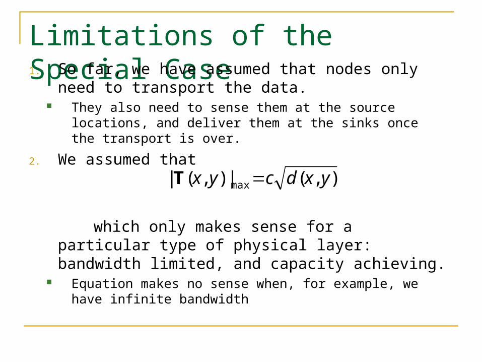
Limitations of the Special Case1. So far, we have assumed that nodes only need to

transport the data. They also need to sense them at the source locations, and

deliver them at the sinks once the transport is over.

2. We assumed that

which only makes sense for a particular type of physical layer: bandwidth limited, and capacity achieving.

Equation makes no sense when, for example, we have infinite bandwidth

),(|),(| max yxdcyx T

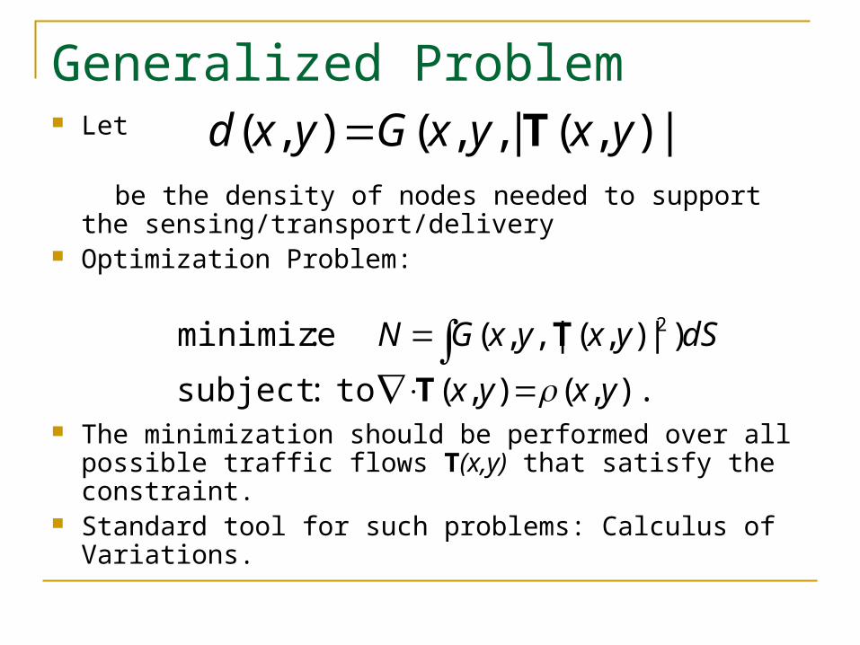
Generalized Problem Let

be the density of nodes needed to support the sensing/transport/delivery

Optimization Problem:

The minimization should be performed over all possible traffic flows T(x,y) that satisfy the constraint.

Standard tool for such problems: Calculus of Variations.

|)),(|,,(),( yxyxGyxd T

).,(),( :subject to

)|),(,|,( :minimize 2

yxyx

dSyxyxGN

T

T

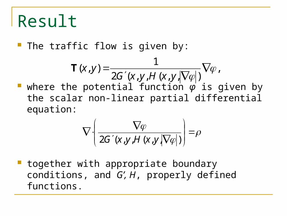
Result The traffic flow is given by:

where the potential function φ is given by the scalar non-linear partial differential equation:

together with appropriate boundary conditions, and G’, H, properly defined functions.

,),,(,,(2

1),(

yxHyxGyxT

),,(,,(2 yxHyxG

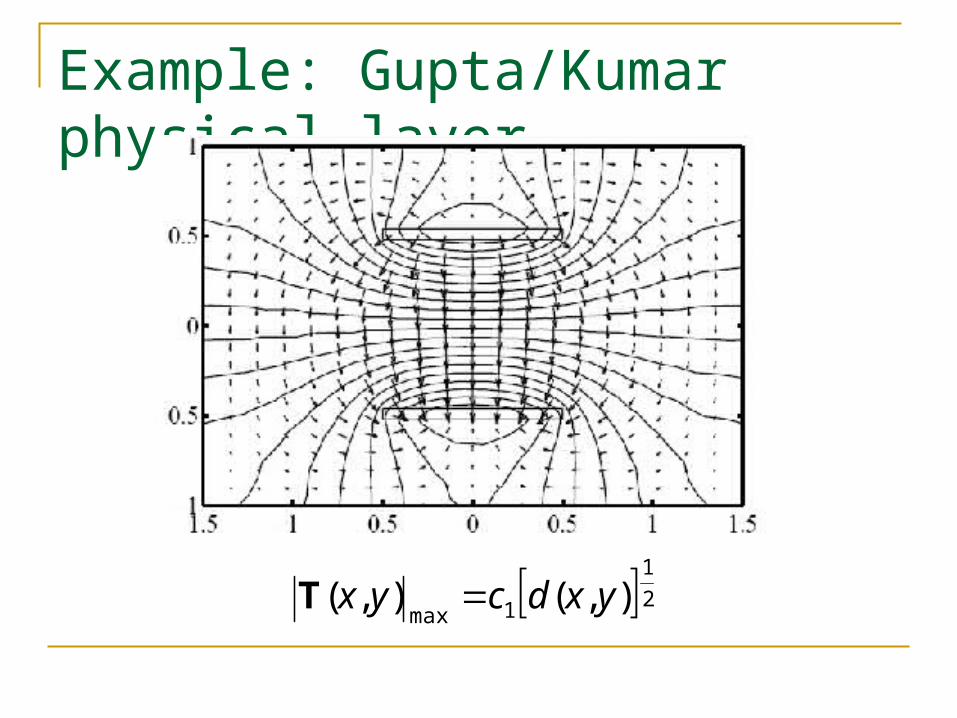
Example: Gupta/Kumar physical layer

21

1max),(),( yxdcyx T

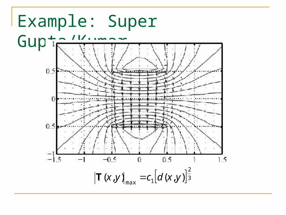
Example: Super Gupta/Kumar

32

1max),(),( yxdcyx T

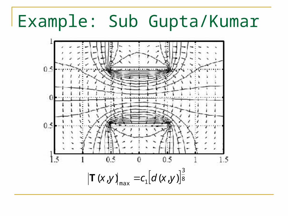
Example: Sub Gupta/Kumar

83

1max),(),( yxdcyx T

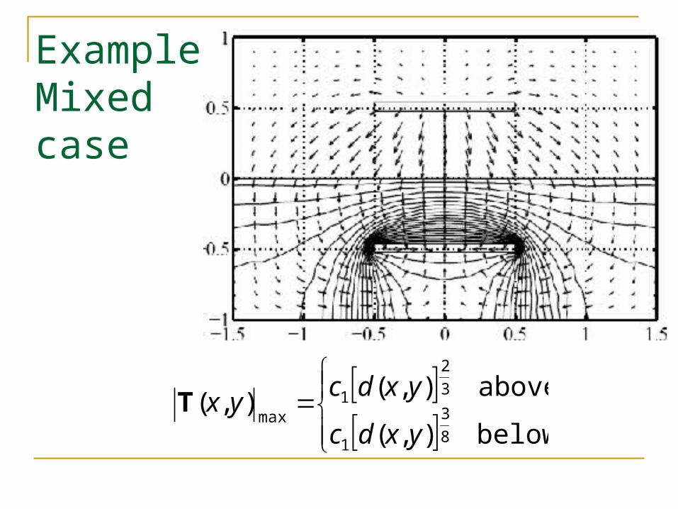
Example: Mixed case

below),(

above),(),(

8

3

1

3

2

1max

yxdc

yxdcyxT

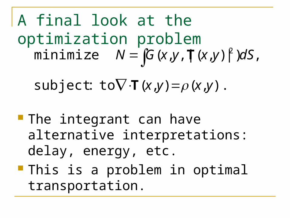
A final look at the optimization problem

).,(),( :subject to

,)|),(,|,( :minimize 2

yxyx

dSyxyxGN

T

T

The integrant can have alternative interpretations: delay, energy, etc.

This is a problem in optimal transportation.

3. “Packetoptics”P. Jacquet, INRIA

R. Catanuto, G. Morabito, University of Catania

S. Toumpis, University of Cyprus

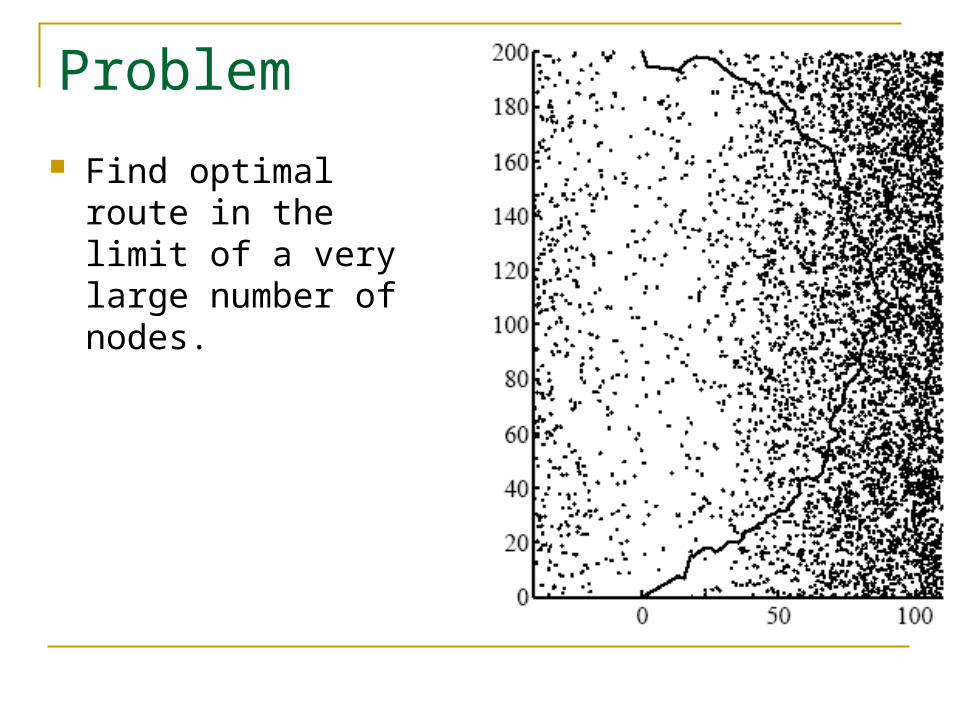
Problem

Find optimal route in the limit of a very large number of nodes.

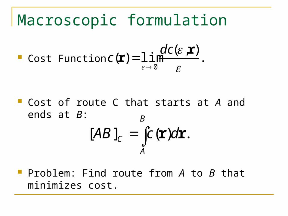
Macroscopic formulation

Cost Function:

Cost of route C that starts at A and ends at B:

Problem: Find route from A to B that minimizes cost.

.),(

lim)(0

rr

dcc

.)(][ B

A

C dcAB rr

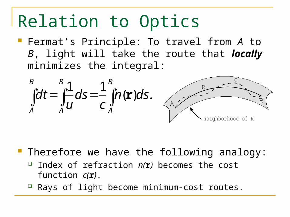
Relation to Optics Fermat’s Principle: To travel from A to B, light will

take the route that locally minimizes the integral:

Therefore we have the following analogy: Index of refraction n(r) becomes the cost function c(r). Rays of light become minimum-cost routes.

.)(11

B

A

B

A

B

A

dsnc

dsu

dt r

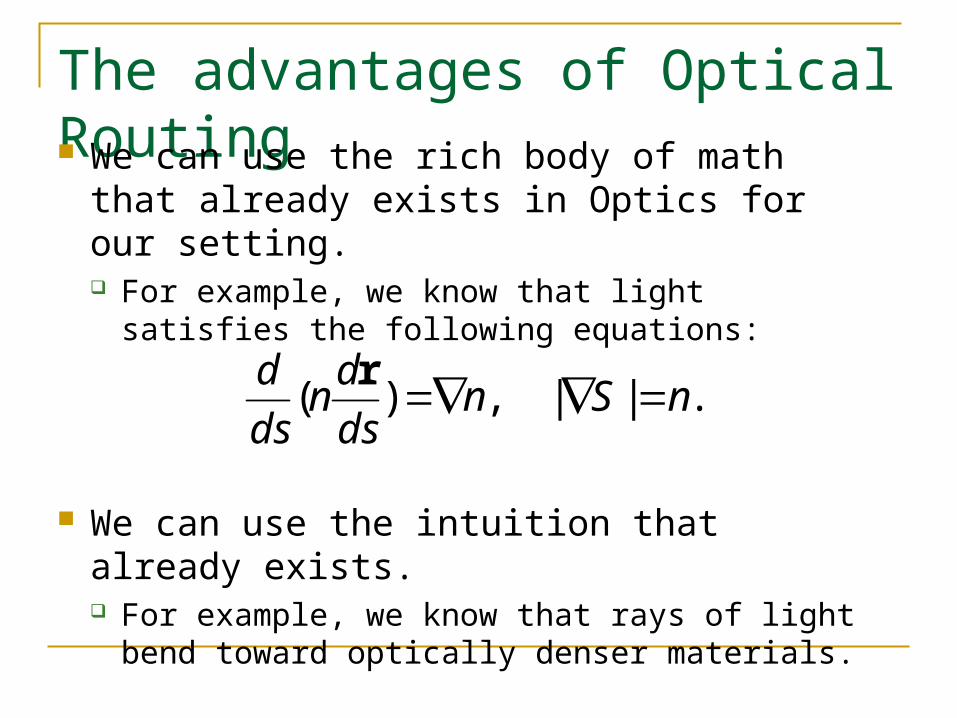
The advantages of Optical Routing We can use the rich body of math that

already exists in Optics for our setting. For example, we know that light satisfies the

following equations:

We can use the intuition that already exists. For example, we know that rays of light bend

toward optically denser materials.

.||,)( nSnds

dn

ds

d

r

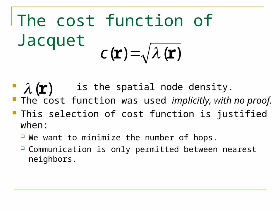
The cost function of Jacquet

)()( rr c

is the spatial node density. The cost function was used implicitly, with no proof. This selection of cost function is justified when:

We want to minimize the number of hops. Communication is only permitted between nearest

neighbors.

)(r

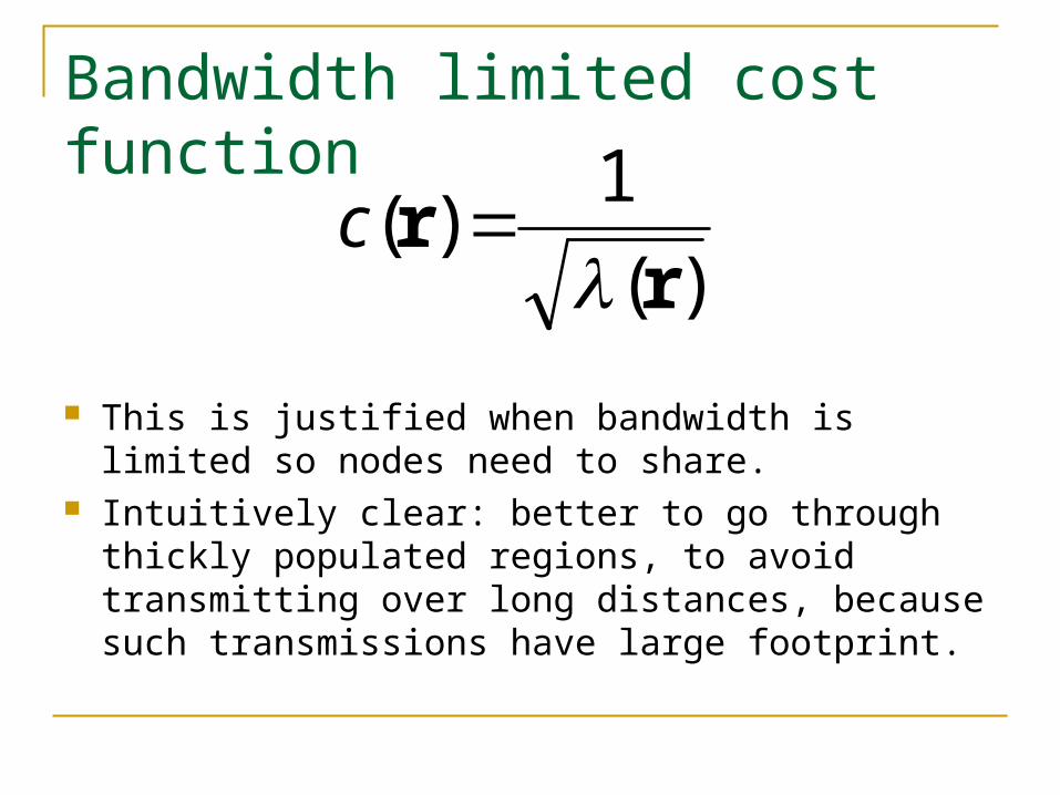
Bandwidth limited cost function

This is justified when bandwidth is limited so nodes need to share.

Intuitively clear: better to go through thickly populated regions, to avoid transmitting over long distances, because such transmissions have large footprint.

)(

1)(

rr

c

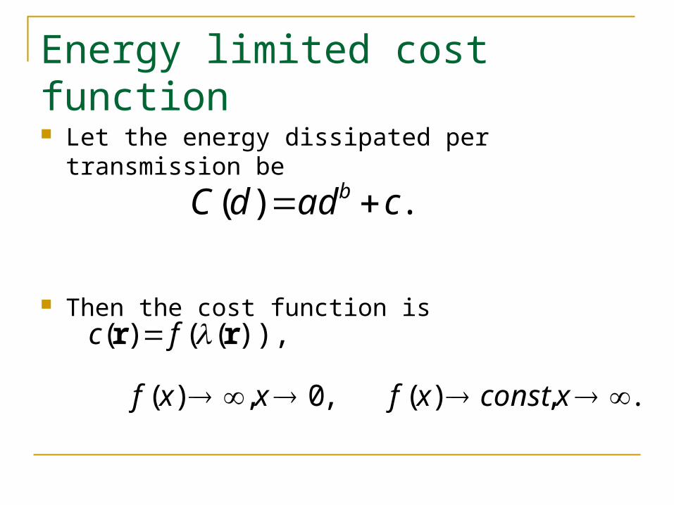
Energy limited cost function

Let the energy dissipated per transmission be

Then the cost function is

.)( caddC b

.,)(,0,)(

)),(()(

xconstxfxxf

fc rr

Other cost functions

Minimize delay Minimize congestion Dynamic cost functions Avoid high levels of interference (Baccelli,

Bambos, Chan, Infocom 2006) Very versatile!!!

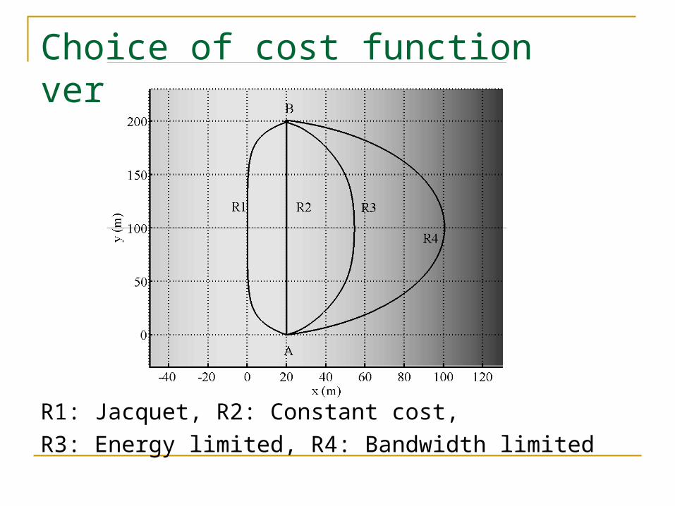
Choice of cost function very important!

R1: Jacquet, R2: Constant cost,

R3: Energy limited, R4: Bandwidth limited

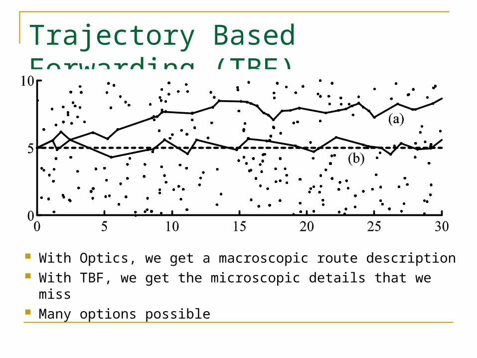
Trajectory Based Forwarding (TBF)

With Optics, we get a macroscopic route description With TBF, we get the microscopic details that we miss Many options possible

What the Optics-Networking Analogy does not tell us How does the source know the initial angle

with which the packet/ray should be launched?

In some nonhomogeneous environments, there are multiple rays connecting two points All of them local minimums One of them global minimum

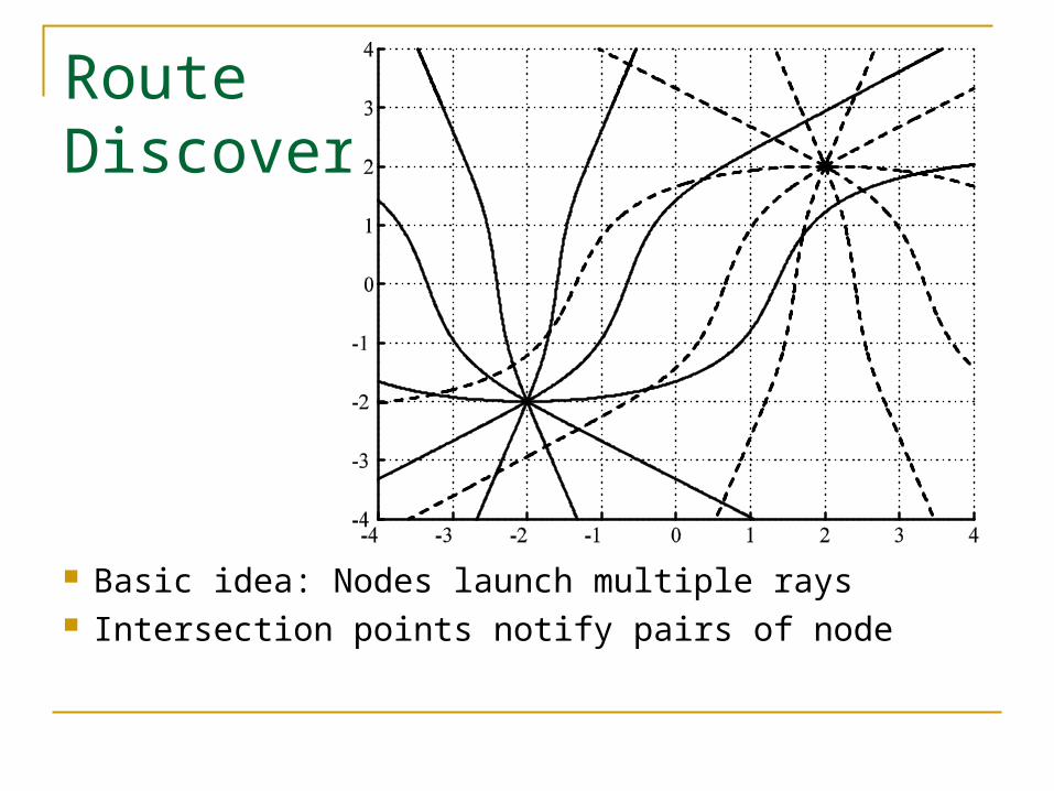
Route Discovery

Basic idea: Nodes launch multiple rays Intersection points notify pairs of node

4. Cooperative TransmissionsB. Sirkeci-Mergen, A. Scalione, Cornell University

Setting Topology: source placed on left side of strip,

destination placed on right side of strip, relays are placed in strip, Poisson distributed.

Reception model: nodes susceptible to thermal noise, power decays with distance as pr(d)=kd-2, reception successful if SINR>γ.

Protocol: We slot time. In first slot, source transmits. In i-th slot, everyone transmits if he received for first time in previous slot. Transmission powers add up at potential receivers.

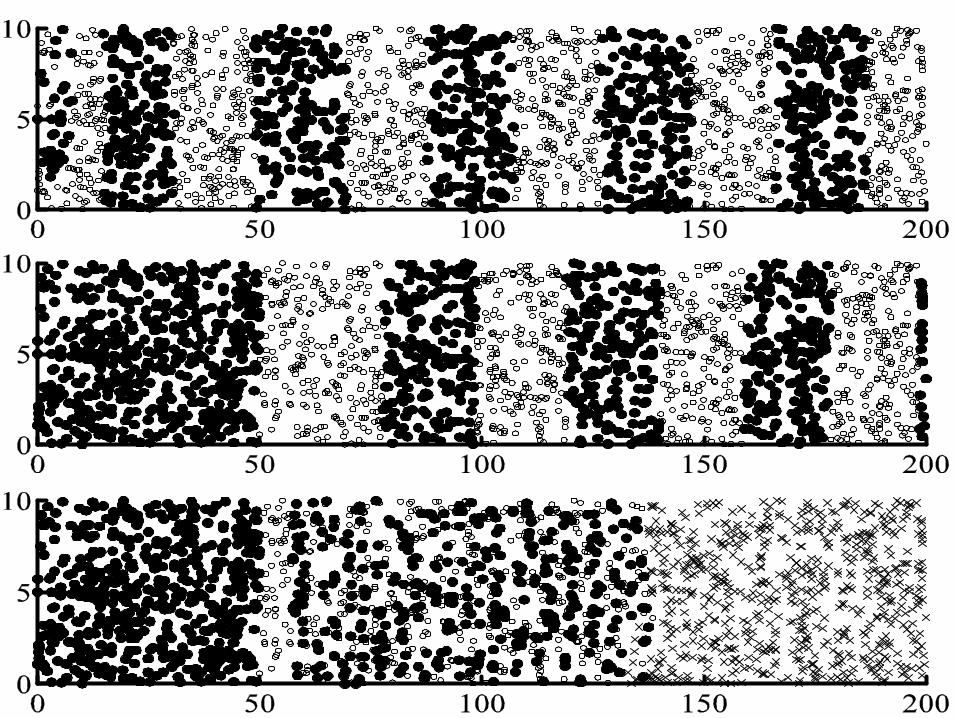
What the simulations say

For sufficiently low threshold, a wave is formed that propagates along the strip. After a while, wave achieves fixed width and goes on for ever.

For high threshold, wave eventually dies out, irrespective of how many nodes initially had the packet.

Position of initial relays critical.

The massively dense assumption Analysis very hard because of random

placement of nodes. Assumption: We have so many nodes, that

there is a node practically everywhere. Not interested in which node receives in i-

th slot. Interested in which region of space

receives in i-th slot.

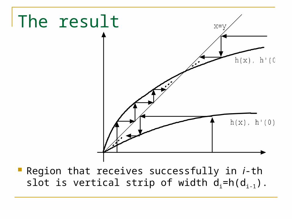
The result

Region that receives successfully in i-th slot is vertical strip of width di=h(di-1).

5. Energy Efficient RoutingM. Kalantari, M. Shayman, University of Maryland

Setting A Wireless Sensor Network with multiple

sources and a central sink. A very large number of nodes

Modeled by node density function. Not subject to optimization.

Problem: Find routes from sources to the sink that are energy efficient.

Intuition: Avoid concentration of traffic in any given location.

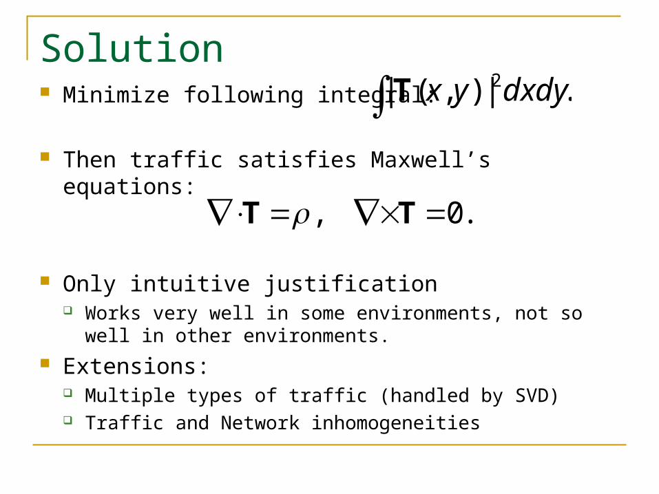
Solution Minimize following integral:

Then traffic satisfies Maxwell’s equations:

Only intuitive justification Works very well in some environments, not so well in

other environments. Extensions:

Multiple types of traffic (handled by SVD) Traffic and Network inhomogeneities

.|),(| 2dxdyyxT

.0 , TT

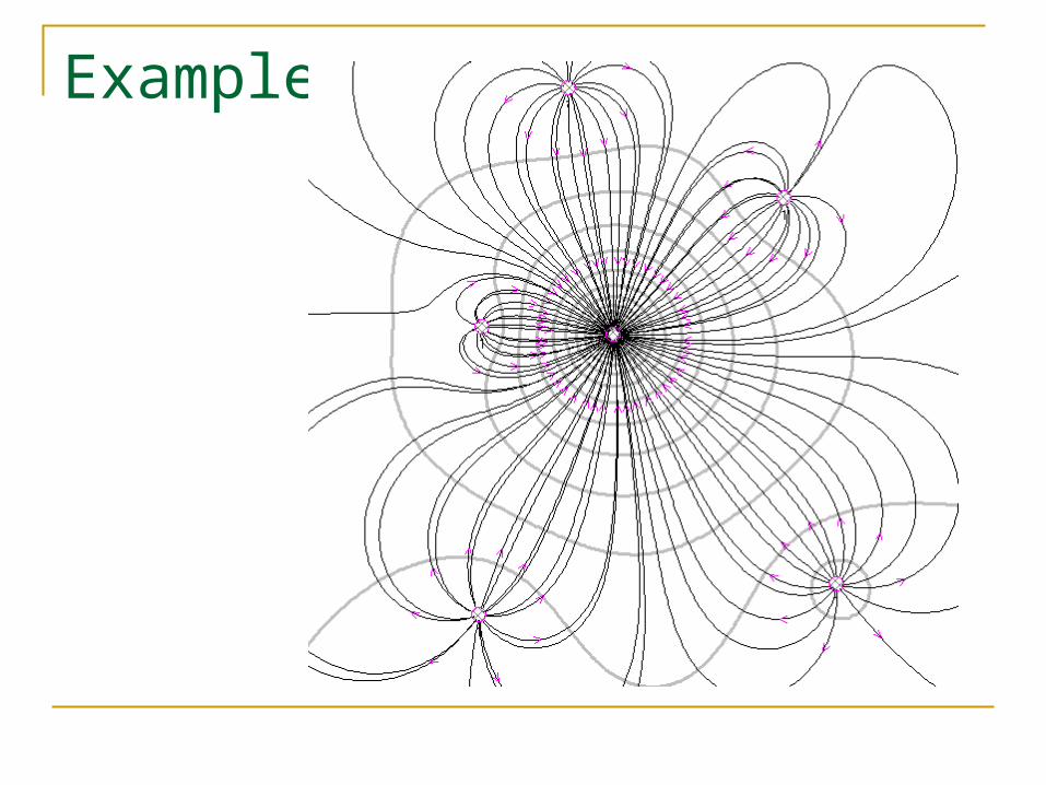
Example

6. Load Balancing

E. Hyytiä, J. Virtamo, University of Helsinki

Setting

Until now, we supposed only one type of traffic, or at most a few.

In general case, if there are n nodes, there will be n(n-1) distinct traffics (and that ignoring multicasting!)

Macroscopic approach: Location r1 creates traffic for location r2 with rate λ(r1,r2), measured in bps/m4.

Problem Formulation Set of all paths is P. Traffic through location r with direction θ has angular

flux Φ(P,r,θ), measured in bps/m/rad. Total volume that passes through location r is given

by scalar flux Φ(P,r):

Problem: Find optimal distribution of paths, so that maximum traffic load is minimized:

.),),2

0

drr PP Φ(Φ(

).,maxargminopt rr PP P Φ(

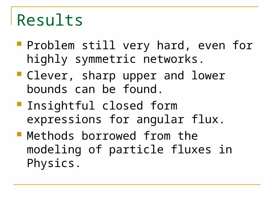
Results Problem still very hard, even for highly

symmetric networks. Clever, sharp upper and lower bounds can be

found. Insightful closed form expressions for angular

flux. Methods borrowed from the modeling of

particle fluxes in Physics.

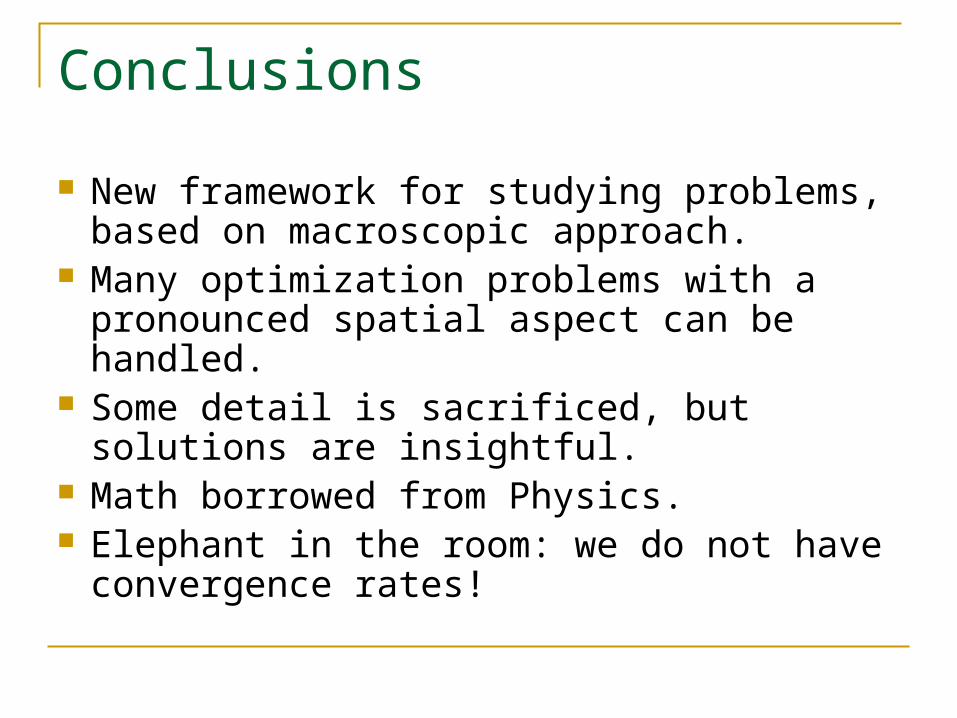
Conclusions

New framework for studying problems, based on macroscopic approach.

Many optimization problems with a pronounced spatial aspect can be handled.

Some detail is sacrificed, but solutions are insightful.

Math borrowed from Physics. Elephant in the room: we do not have

convergence rates!

References (in chronological order)1. M. Kalantari and M. Shayman, “Energy efficient routing in wireless sensor

networks,” in Proc. CISS, Princeton University, NJ, Mar. 2004.2. P. Jacquet, “Geometry of information propagation in massively dense ad

hoc networks, in Proc. ACM MobiHOC, Roppongi Hills, Japan, 20043. M. Kalantari and M. Shayman, “Routing in wireless ad hoc networks by

analogy to electrostatic theory,” in Proc. IEEE ICC, 2004.4. P. Jacquet, “Space-time information propagation inmobile ad hoc wireless

networks,” in Proc. Information Theory Workshop, San Antonio, TX, Oct. 2004.

5. S. Toumpis and L. Tassiulas, “Packetostatics: Deployment of massively dense sensor networks as an electrostatics problem,” in Proc. IEEE Infocom 2005

6. B. Sirkeci-Mergen and A. Scaglione, “A continuum approach to dense wireless networks with cooperation,” in Proc. Infocom 2005

7. S. Toumpis and G. A. Gupta, “Optimal placement of nodes in large sensor networks under a general physical layer model,”, in Proc. IEEE SECON 2005.

8. M. Kalantari and M. Shayman, “Routing in multi-commodity sensor networks based on partial differential equation,” in Proc. Conference on Information Sciences and Systems, Princeton University, NJ, Mar 2006

9. M. Kalantari and M. Shayman, “Design optimization of multi-sink sensor networks by analogy to electrostatic theory,” in Proc. WCNC, Las Vegas, NV, Apr. 2006

10. E. Hyytiä and J. Virtamo, “On load balancing in a dense wireless multihop network,” in Proc. 2nd EuroNGI Conference on Next Generation Internet Design and Engineering (NGI 2006), Valencia, Spain, Apr. 2006.

11. F. Baccelli, N. Bambos, and C. Chan, “Optimal power, throughput, and routing for wireless link arrays,” in Proc. IEEE Infocom, 2006.

12. R. Catanuto and G. Morabito, “Optimal routing in dense wireless multihop networks as a geometrical optics solution to the problem of variations,” in Proc. IEEE ICC, Istanbul, Turkey, June 2006.

13. B. Sirkeci-Mergen, A. Scaglione, and G. Mergen, “Asymptotic analysis of multistage cooperative broadcast in wireless networks,” IEEE Trans. Inform. Theory, vol. 52, no. 6, pp. 2531-2550.

14. S. Toumpis and L. Tassiulas, “Optimal deployment of large wireless sensor networks, “ IEEE Trans. Inform. Theory, July 2006.

15. R. Catanuto, G. Morabito, and S. Toumpis, “Optical Routing in massively dense networks: Practical issues and dynamic programming interpretation,” in Proc. International Symposium on Wireless Communication Systems, Valencia, Spain, 2006.

16. B. Sirkeci-Mergen and A. Scaglione, “On the power efficiency of cooperative broadcast in dense wireless networks,” submitted to IEEE Journal on Selected Areas in Communication (JSAC), Feb. 2006.

17. R. Catanuto, S. Toumpis, and G. Morabito, “Opti{c,m}al routing in massively dense wireless networks,” submitted for publication, available as technical note in arXiv.