Stats Formulas &Tables

8/10/2019 Stats Formulas &Tables

http://slidepdf.com/reader/full/stats-formulas-tables 1/21

Statistical Formulas and Tables

for use with

STAT1010: Riippuvuusanalyysi

Bernd Papehttp://www.uwasa.fi/∼bepa/

Measures of Contingency

Pearson’s χ2:

χ2 =r

i=1

sj=1

(f ij − eij)2

eij, (1)

wheref ij are the observed frequencies in cell (i,j), and

eij = f i•f •j

n

with f i• = j f ij and f •j = i f ij

are the expected frequencies in cell (i,j) under independenceof r row variables and s column variables.

Contingency Coefficient:

C =

χ2

χ2 + n with maximum C max =

k − 1

k , (2)

where k is the smaller number of the rows r and columns s.

Cramer’s V :

V =

χ2

χ2max, where χ2max = n(k − 1) (3)

is the largest possible value of Pearson’s χ2-statistic in a table with r rows



Kendall’s rank correlation τ :

τ = 1− 4Q

n(n− 1), (5)

where Q is the number of discordant pairs within n observation pairs.

χ2

-based Testsχ2 independence test:

χ2 =r

i=1

sj=1

(f ij − eij)2

eij∼ χ2((r − 1)(s− 1)) under (6)

H 0 : X and Y are statistically independent

Continuity adjustment for two-way tables, that is r = s = 2:

χ2 = n(|f 11f 22 − f 12f 21| − n/2)2

f 1•f 2•f •1f •2∼ χ2(1) under H 0 (7)

with f ij observed frequencies in cell (i,j), f i• = f i1+f i2, and f •j = f 1j+f 2j .

χ2-test for equality of proportions:

χ2 independence test upon the following contingency table,

sample 1 · · · sample k sumsuccess n1 p1 · · · nk pk f 1• =

ni pi

failure n1(1 − p1) · · · nk(1 − pk) f 2• =

ni(1 − pi)sum: f •1 = n1 · · · f •k = nk n =

ni

with ni = size of sample i, and pi = proportion of success in sample i.

Median test:

χ2 independence test with expected frequencies eij = ni/2,where ni is the sample size from population i.

McNemar test on paired proportions:



Nonparametric Tests

Sign Test:

With n observation pairs (xi, yi), the test statistic is T = number of plussigns, where xi > yi → (+) and xi < yi → (−) and pairs with xi = yi (ties)are discarded.

Under H 0 : P (X > Y ) = 1

2, T ∼ Bin

n,

1

2

. (9)

For n →∞ : Z = 2T − n√

n ∼ N (0, 1) under H 0. (10)

Wilcoxon Signed-Rank Test:

The hypotheses of the two-sided test for paired observations areH 0 : median of population 1 = median of population 2,H 1 : median of population 1 = median of population 2.

The Wilcoxon T statistic is defined as the smaller of the two sums of ranks,

T = min

(+),

(−)

,

where (+/

−) is the sum of the ranks of the positive/negative differences of

the observation pairs (x1, x2). We reject the null hypothesis of the two-sidedtest if the computed value of the statistic is less than the α

2 critical point from

the table. We reject H 0 against the one-sided alternative

H 1 : median of population 1 > (<) median of population 2

if

(−) (

(+)) is less than the α critical point from the table.

Kruskal-Wallis Test

Let ni, i = 1, . . . , k denote the sample size from population i and let n =n1 + · · ·+ nk. Defining Ri, i = 1, . . . , k as the sum of ranks from sample k , theKruskal-Wallis test statistic is

H = 12

n(n + 1)

ki 1

R2i

ni− 3(n + 1) ∼ χ2(k − 1) under (11)



with test statistic: R = number of runs. For large sample sizes n = n+ + n−:

z = R− E (R)

σr∼ N (0, 1) under H 0, where (12)

E (R) = 2n+n−

n

+ 1, σR = 2n+n−(2n+n− − n)

n2

(n− 1)

(13)

We reject H 0 at significance level α if |z| > z (α2

).

Principles of ANOVA

Consider k independent samples:

x11, x12, . . . , x1n1 ,

...

xk1, xk2, . . . , xknk,

where xij ∼ N (µi, σ2) and n1 + · · · + nk = N . We wish to test whether allobservations come from the same distribution or not.

1) The Sum of Squares Principle

grand mean: x = 1

N

ki=1

nij=1

xij = 1

N

ki=1

nixi (14)

SST =i

j

(xij − x)2 = (N − 1)s2 (15)

= i

ni(xi−x)2

j (xi − x)

2

+i

(ni−1)s2

i

j (xij − xi)

2

(16)

= SSB + SSE (17)

where xi and s2i are the mean and the sample variance of the observations inthe i’th sample, and s2 is the sample variance of all observations.



3) The Mean Squares and the F -test

F = M SB

MSE ∼ F (k−1, N −k) under (19)

H 0 : µ1 = µ2 = . . . = µk, where

MSB = SSB

DFB

and MSE = SSE

DFE

. (20)

4) Estimation of the effects

Fixed effects model: ai = xi − x, i = 1, 2, . . . k . (21)

Random effects model: s2A = MSB− MSE

n0with (22)

n0 = N 2 −

ki=1 n2i

N (k − 1)

, (23)

where n0 = n in the special case of equal sample sizes n = N/k in all groups.

ContrastsQ

MSE ∼ F (1, DFE) and t =

L

s(L) ∼ t(DFE) where (24)

L = λixi, Q = L

2λ2i /ni

, and s(L) = MSE λ

2

ini

(25)

under H 0 : λ1µ1 + λ2µ2 + · · ·+ λkµk = 0,

where λ1 + λ2 + · · · + λk = 0.

Two contrasts ψ1/2 =

ki=1

λ1/2iµi with

ki=1

λ1/2i = 0 are orthogonal if

ki=1

λ1iλ2ini

= 0. (26)

Simultaneous Confidence Intervals

CI 1−α = [(xi − xj) ± smallest significant difference], (27)



Two-Way ANOVA

Consider taking independent samples from data which is split into I × J pop-ulations according to I levels of factor A and J levels according to factor B.Denote with X ijk the k’th observation of the sample corresponding to level i of factor A and level j of factor B and assume

X ijk = μ + αi + β j + (αβ )ij + ijk , ijk ∼N (0,σ2), (31)

such thatI

i=1

αi =J j=1

β j =I

i=1

J j=1

(αβ )ij = 0. (32)

ANOVA Table for Two-Way Analysis

Source of Sum of Degrees MeanVariation Squares of Freedom Square F Ratio

Factor A SSA I − 1 MSA= SSA

I − 1 F =

MSA

MSE

Factor B SSB J − 1 MSB= SSB

J − 1 F =

MSB

MSE

Interaction SSAB (I − 1)(J − 1) MSAB= SSAB

(I − 1)(J − 1) F =

MSABMSE

Error SSE N − IJ MSE= SSE

N − IJ

Total SST N − 1

where N denotes the total number of observations.

Hypothesis Tests in Two-Way ANOVA

Factor A main-eff ects test:

F = MSA/MSE ∼ F (I − 1, N − IJ ) (33)

d H 0 f ll i 1 I



ANOVA Table for Randomized Complete Block Design

Consider k treatments, which are randomly assigned to b blocks.

Source of Sum of Degrees MeanVariation Squares of Freedom Square F Ratio

Blocks SSBL b− 1 MSBL= SSBL

b− 1

Treatments SSTR k − 1 MSTR= SSTR

k − 1 F =

MSTR

MSE

Error SSE (k − 1)(b− 1) MSE= SSE

(k

−1)(b

−1)

Total SST kb − 1

Hypothesis Test in Randomized Complete Block Design

F = MSTR

MSE ∼ F (k − 1, (k − 1)(b− 1)) (36)

under H 0 : μ1 = μ2 = · · · = μk.

Linear Correlation and Regression

Pearsons Linear Correlation Coefficient

T = r√

n− 2√ 1− r2

∼ t(n− 2) under (37)

H 0 : ρ = 0 (x, y are linearly independent).

For large n and small r approximately:

Z = r√

n− 1 ∼ N (0, 1) under H 0, (38)

where r is the sample linear correlation coefficient and n is the number of obser-vation pairs. The same test may in large samples be used to assess H 0 : ρS = 0or τ =0 by replacing r with Spearmans rank correlation rS or Kendall’s τ



Sample representation of linear regression in matrix form:

y(n×1)

= X(n×(k+1))

b((k+1)×1)

+ u(n×1)

, with

X =

⎛

⎜⎜⎜⎝

1 x1,1 x2,1 · · · xk,11 x1,2 x2,2 · · · xk,2...

......

...

1 x1,n x2,n · · · xk,n

⎞

⎟⎟⎟⎠, b =

⎛

⎜⎜⎜⎝

b0b1...

bk

⎞

⎟⎟⎟⎠, (40)

y = (y1, y2, . . . , yn) and u = (u1, u2, . . . , un).

Least-square estimates for β 0, . . . ,β k:

β ((k+1)×1) = b = (XX)−1Xy (41)

In the special case of only 1 regressor:

b1 = rxy ·

sysx and b0 = y − b1x, (42)

where rxy denotes the sample correlation coefficient and x, y and sx, sy denotethe arithmetic means and standard deviations of x and y , respectively.

t-test for single regression parameters:

t = bi − β ∗i

SE bi∼ t(n−k−1) under H 0 : β i = β ∗i , (43)

where SE bi−1 =

MSE(XX)−1ii (44)

with MSE = SSE

n− (k + 1) =

(yj − yj)2

n− (k + 1) . (45)


SE b1 =

MSE

SSX and SE b0 =

MSE

1

n +

x2

SS X

, (46)

where SSX =ni=1

(xi − x)2. (47)

In particular for β ∗i = 0:

t = biSE

∼ t(n−k−1) under H 0 : β i = 0. (48)



Prediction interval on individual response at x:

CI (1−α) =

Y |x ± tα2

(n−k−1)

MSE · (1 + x(XX)−1x)

, (51)

where x = (1, x1, x2, . . . , xk).


CI (1−α) = y ± tα/2(n−2) ·

MSE

1 +

1

n +

(x− x)2

SSX

. (52)

ANOVA Table for Multiple Regression

Source Sum of Squares DF Mean Square F Ratio

Regression SSR=(yi − y)2 k SSR/DFR MSR/MSE

Error SSE=

(yi − yi)2 n− (k+1) SSE/DFE

Total SST=

(yi − y)2 n− 1 SST/DFT

where n is the number of observation tuples and k is the number of regressors(excluding the intercept).

The ANOVA F-test for Multiple Regression

The ratio MSRMSE is an F statistic for testing

H 0 : β 1 = β 2 = · · · = β k = 0

againstH 1 : Not all β i, i = 1, . . . , k are zero.

Under H 0: F = MSR

MSE =

SSR/k

SSE/(n−

k−

1) ∼ F (k, n− k − 1) (53)

and F = R2

1−R2 ·

n − (k + 1)

k ∼ F (k, n− k − 1). (54)

The coefficient of determination R2:

R2 r2s2y SSR

1 SSE

(55)



The partial F-test for adding/deleting regressors

Consider the full regression model

Y = β 0 + β 1X 1 + β 2X 2 + · · · + β kX k +

with sum of squared residuals SS E F and mean square error MSE F as an al-

ternative to the reduced modelY = β 0 + β 1X 1 + β 2X 2 + · · · + β k−rX k−r +

with sum of squared residuals S SE R. Then

F = (SSE R − SS E F )/r

MSE F ∼ F (r, n−(k+1)) (57)

under H 0 : β k−r+1 = β k−r+2 = . . . = β k = 0.

The Durbin-Watson test

In order to test for first order autocorrelation ρ1 at significance level α:

1. Choose a significance level (e.g. α= 0.05).

2. Calculate d =

ni=2(ei − ei−1)2

ni=1 e2i

≈ 2(1− ρ1).

3. Look up:dL(α2 ) and dU (

α2 ) for a two-sided test,

dL(α) and dU (α) for a one-sided test.

4. (i) Two-sided: H 0 : ρ1=0 vs. H 1 : ρ1= 0d ≤ dL or d ≥ 4−dL ⇒ reject H 0.dU ≤ d ≤ 4−dU ⇒ accept H 0.otherwise ⇒ inconclusive.

(ii) One-sided: H 0 : ρ1=0 vs. H 1 : ρ1> 0d ≤ dL ⇒ reject H 0.d ≥ dU ⇒ accept H 0.otherwise ⇒ inconclusive.

(iii) One-sided: H 0 : ρ1=0 vs. H 1 : ρ1< 0d ≥ 4− dL ⇒ reject H 0.d ≤ 4− dU ⇒ accept H0.



Logistic Regression

The binary logistic regression model is

log

p

1− p

= β 0 + β 1x, (59)

where p is the probability of success and x is the explanatory variable.

The probability of success is then given by the logistic function

p = 1

1 + e−(β0+β1x). (60)

Confidence Intervals for logistic regression:

A level α confidence interval for β 1 (slope) is

CI (1−α) = b1 ± zα/2SE b1 . (61)

A level α confidence interval for the odds ratio eβ1 is

CI (1−α) =

eb1−zα/2SEb1 , eb1+zα/2SEb1

. (62)

Significance tests for logistic regression:

z = b1SE b1

∼ N (0, 1) and z2 =

b1SE b1

2 ∼ χ2(1) under H 0 : β 1 = 0. (63)



Wilcoxon Signed-Rank Test:

The table below displays the integer numbers which cor-

respond most closely to the critical values t p of rejecting

equal medians in one-sided Wilcoxon Signed-Rank tests

at significance level p. n denotes the number of observa-tion pairs.

p : 0.05 0.025 0.01 0.005

2 p : 0.10 0.05 0.02 0.01

n = 6 2 1

7 4 2 0

8 6 4 2 0

9 8 6 3 2

10 11 8 5 3

11 14 11 7 5

12 17 14 10 7

13 21 17 13 10

14 26 21 16 13

15 30 25 20 16

16 36 30 24 19

17 41 35 28 23

18 47 40 33 28





Critical Values q(k,N-k) of the Studentized Range Distribution for alpha=0.05:

N-k: \ k: 2 3 4 5 6 7 8 9 10

1 17.96 26.96 32.81 37.06 40.39 43.10 45.39 47.37 49.09

2 6.08 8.33 9.80 10.88 11.73 12.43 13.03 13.54 13.99

3 4.50 5.91 6.82 7.50 8.04 8.48 8.85 9.18 9.46

4 3.93 5.04 5.76 6.29 6.71 7.05 7.35 7.60 7.83

5 3.64 4.60 5.22 5.67 6.03 6.33 6.58 6.80 6.99

6 3.46 4.34 4.90 5.30 5.63 5.90 6.12 6.32 6.49

7 3.34 4.16 4.68 5.06 5.36 5.61 5.82 6.00 6.16

8 3.26 4.04 4.53 4.89 5.17 5.40 5.60 5.77 5.92

9 3.20 3.95 4.41 4.76 5.02 5.24 5.43 5.59 5.74

10 3.15 3.88 4.33 4.65 4.91 5.12 5.30 5.46 5.60

11 3.11 3.82 4.26 4.57 4.82 5.03 5.20 5.35 5.4912 3.08 3.77 4.20 4.51 4.75 4.95 5.12 5.27 5.39

13 3.06 3.73 4.15 4.45 4.69 4.88 5.05 5.19 5.32

14 3.03 3.70 4.11 4.41 4.64 4.83 4.99 5.13 5.25

15 3.01 3.67 4.08 4.37 4.59 4.78 4.94 5.08 5.20

16 3.00 3.65 4.05 4.33 4.56 4.74 4.90 5.03 5.15

17 2.98 3.63 4.02 4.30 4.52 4.70 4.86 4.99 5.11

18 2.97 3.61 4.00 4.28 4.49 4.67 4.82 4.96 5.07

19 2.96 3.59 3.98 4.25 4.47 4.65 4.79 4.92 5.0420 2.95 3.58 3.96 4.23 4.45 4.62 4.77 4.90 5.01

24 2.92 3.53 3.90 4.17 4.37 4.54 4.68 4.81 4.92

30 2.89 3.49 3.85 4.10 4.30 4.46 4.60 4.72 4.82

40 2.86 3.44 3.79 4.04 4.23 4.39 4.52 4.63 4.73

60 2.83 3.40 3.74 3.98 4.16 4.31 4.44 4.55 4.65

120 2.80 3.36 3.68 3.92 4.10 4.24 4.36 4.47 4.56

Infinity 2.77 3.31 3.63 3.86 4.03 4.17 4.29 4.39 4.47

Critical Values q(k,N-k) of the Studentized Range Distribution for alpha=0.01:

N-k: \ k: 2 3 4 5 6 7 8 9 10

1 89.99 134.77 163.93 185.22 201.80 215.28 226.60 236.34 244.88

2 14.04 19.02 22.29 24.72 26.63 28.20 29.53 30.68 31.69

3 8.26 10.62 12.17 13.32 14.24 15.00 15.64 16.20 16.69

4 6.51 8.12 9.17 9.96 10.58 11.10 11.54 11.93 12.26

5 5.70 6.98 7.80 8.42 8.91 9.32 9.67 9.97 10.24

6 5.24 6.33 7.03 7.56 7.97 8.32 8.61 8.87 9.107 4.95 5.92 6.54 7.00 7.37 7.68 7.94 8.17 8.37

8 4.75 5.64 6.20 6.62 6.96 7.24 7.47 7.68 7.86

9 4.60 5.43 5.96 6.35 6.66 6.91 7.13 7.33 7.49

10 4.48 5.27 5.77 6.14 6.43 6.67 6.87 7.05 7.21

11 4.39 5.15 5.62 5.97 6.25 6.48 6.67 6.84 6.99



The Standard Normal Distribution ©

Example. P (Z ≤ 1.34) = ©(1.34) = 0.9099.

z 0.00 0.01 0.02 0.03 0.04 0.05 0.06 0.07 0.08 0.09

0.0 0.5000 0.5040 0.5080 0.5120 0.5160 0.5199 0.5239 0.5279 0.5319 0.5359

0.1 0.5398 0.5438 0.5478 0.5517 0.5557 0.5596 0.5636 0.5675 0.5714 0.5753

0.2 0.5793 0.5832 0.5871 0.5910 0.5948 0.5987 0.6026 0.6064 0.6103 0.6141

0.3 0.6179 0.6217 0.6255 0.6293 0.6331 0.6368 0.6406 0.6443 0.6480 0.6517

0.4 0.6554 0.6591 0.6628 0.6664 0.6700 0.6736 0.6772 0.6808 0.6844 0.6879

0.5 0.6915 0.6950 0.6985 0.7019 0.7054 0.7088 0.7123 0.7157 0.7190 0.7224

0.6 0.7257 0.7291 0.7324 0.7357 0.7389 0.7422 0.7454 0.7486 0.7517 0.7549

0.7 0.7580 0.7611 0.7642 0.7673 0.7704 0.7734 0.7764 0.7794 0.7823 0.7852

0.8 0.7881 0.7910 0.7939 0.7967 0.7995 0.8023 0.8051 0.8078 0.8106 0.8133

0.9 0.8159 0.8186 0.8212 0.8238 0.8264 0.8289 0.8315 0.8340 0.8365 0.8389

1.0 0.8413 0.8438 0.8461 0.8485 0.8508 0.8531 0.8554 0.8577 0.8599 0.8621

1.1 0.8643 0.8665 0.8686 0.8708 0.8729 0.8749 0.8770 0.8790 0.8810 0.8830

1.2 0.8849 0.8869 0.8888 0.8907 0.8925 0.8944 0.8962 0.8980 0.8997 0.9015

1.3 0.9032 0.9049 0.9066 0.9082 0.9099 0.9115 0.9131 0.9147 0.9162 0.9177

1.4 0.9192 0.9207 0.9222 0.9236 0.9251 0.9265 0.9279 0.9292 0.9306 0.9319

1.5 0.9332 0.9345 0.9357 0.9370 0.9382 0.9394 0.9406 0.9418 0.9429 0.94411.6 0.9452 0.9463 0.9474 0.9484 0.9495 0.9505 0.9515 0.9525 0.9535 0.9545

1.7 0.9554 0.9564 0.9573 0.9582 0.9591 0.9599 0.9608 0.9616 0.9625 0.9633

1.8 0.9641 0.9649 0.9656 0.9664 0.9671 0.9678 0.9686 0.9693 0.9699 0.9706

1.9 0.9713 0.9719 0.9726 0.9732 0.9738 0.9744 0.9750 0.9756 0.9761 0.9767

2.0 0.9772 0.9778 0.9783 0.9788 0.9793 0.9798 0.9803 0.9808 0.9812 0.9817

2.1 0.9821 0.9826 0.9830 0.9834 0.9838 0.9842 0.9846 0.9850 0.9854 0.9857

2.2 0.9861 0.9864 0.9868 0.9871 0.9875 0.9878 0.9881 0.9884 0.9887 0.9890

2.3 0.9893 0.9896 0.9898 0.9901 0.9904 0.9906 0.9909 0.9911 0.9913 0.9916

2.4 0.9918 0.9920 0.9922 0.9925 0.9927 0.9929 0.9931 0.9932 0.9934 0.9936

2.5 0.9938 0.9940 0.9941 0.9943 0.9945 0.9946 0.9948 0.9949 0.9951 0.9952

2.6 0.9953 0.9955 0.9956 0.9957 0.9959 0.9960 0.9961 0.9962 0.9963 0.9964

2.7 0.9965 0.9966 0.9967 0.9968 0.9969 0.9970 0.9971 0.9972 0.9973 0.9974

2.8 0.9974 0.9975 0.9976 0.9977 0.9977 0.9978 0.9979 0.9979 0.9980 0.9981

2 9 0 9981 0 9982 0 9982 0 9983 0 9984 0 9984 0 9985 0 9985 0 9986 0 9986

ΦΦΦΦ(z) = P(Z < z)

Second decimal of z



Table. Tail fractiles (tα) of the t-distribution: P (T > tα(df )) = α.



Table. Tail fractiles χ2α of the χ2-distribution: P (χ2>χ2

α(df )) =α.

df / α 0.995 0.990 0.975 0.950 0.900 0.100 0.050 0.025 0.010 0.001

1 0.000039 0.000157 0.000982 0.003932 0.0158 2.706 3.841 5.024 6.635 10.827

2 0.0100 0.0201 0.0506 0.103 0.211 4.605 5.991 7.378 9.210 13.8153 0.0717 0.115 0.216 0.352 0.584 6.251 7.815 9.348 11.345 16.266

4 0.207 0.297 0.484 0.711 1.064 7.779 9.488 11.143 13.277 18.466

5 0.412 0.554 0.831 1.145 1.610 9.236 11.070 12.832 15.086 20.515

6 0.676 0.872 1.237 1.635 2.204 10.645 12.592 14.449 16.812 22.457

7 0.989 1.239 1.690 2.167 2.833 12.017 14.067 16.013 18.475 24.321

8 1.344 1.647 2.180 2.733 3.490 13.362 15.507 17.535 20.090 26.124

9 1.735 2.088 2.700 3.325 4.168 14.684 16.919 19.023 21.666 27.877

10 2.156 2.558 3.247 3.940 4.865 15.987 18.307 20.483 23.209 29.58811 2.603 3.053 3.816 4.575 5.578 17.275 19.675 21.920 24.725 31.264

12 3.074 3.571 4.404 5.226 6.304 18.549 21.026 23.337 26.217 32.909

13 3.565 4.107 5.009 5.892 7.041 19.812 22.362 24.736 27.688 34.527

14 4.075 4.660 5.629 6.571 7.790 21.064 23.685 26.119 29.141 36.124

15 4.601 5.229 6.262 7.261 8.547 22.307 24.996 27.488 30.578 37.698

16 5.142 5.812 6.908 7.962 9.312 23.542 26.296 28.845 32.000 39.252

17 5.697 6.408 7.564 8.672 10.085 24.769 27.587 30.191 33.409 40.791

18 6.265 7.015 8.231 9.390 10.865 25.989 28.869 31.526 34.805 42.312

19 6.844 7.633 8.907 10.117 11.651 27.204 30.144 32.852 36.191 43.81920 7.434 8.260 9.591 10.851 12.443 28.412 31.410 34.170 37.566 45.314

21 8.034 8.897 10.283 11.591 13.240 29.615 32.671 35.479 38.932 46.796

22 8.643 9.542 10.982 12.338 14.041 30.813 33.924 36.781 40.289 48.268

23 9.260 10.196 11.689 13.091 14.848 32.007 35.172 38.076 41.638 49.728

24 9.886 10.856 12.401 13.848 15.659 33.196 36.415 39.364 42.980 51.179

25 10.520 11.524 13.120 14.611 16.473 34.382 37.652 40.646 44.314 52.619

26 11.160 12.198 13.844 15.379 17.292 35.563 38.885 41.923 45.642 54.051

27 11.808 12.878 14.573 16.151 18.114 36.741 40.113 43.195 46.963 55.47528 12.461 13.565 15.308 16.928 18.939 37.916 41.337 44.461 48.278 56.892

29 13.121 14.256 16.047 17.708 19.768 39.087 42.557 45.722 49.588 58.301

30 13.787 14.953 16.791 18.493 20.599 40.256 43.773 46.979 50.892 59.702

40 20.707 22.164 24.433 26.509 29.051 51.805 55.758 59.342 63.691 73.403

50 27.991 29.707 32.357 34.764 37.689 63.167 67.505 71.420 76.154 86.660

60 35 534 37 485 40 482 43 188 46 459 74 397 79 082 83 298 88 379 99 608

χα2(df)



F0.1(m,n)

n \m 1 2 3 4 5 6 7 8 9 10 15 30 40 60 120

1 39.86 49.50 53.59 55.83 57.24 58.20 58.91 59.44 59.86 60.19 61.22 62.26 62.53 62.79 63.06

2 8.53 9.00 9.16 9.24 9.29 9.33 9.35 9.37 9.38 9.39 9.42 9.46 9.47 9.47 9.48

3 5.54 5.46 5.39 5.34 5.31 5.28 5.27 5.25 5.24 5.23 5.20 5.17 5.16 5.15 5.14

4 4.54 4.32 4.19 4.11 4.05 4.01 3.98 3.95 3.94 3.92 3.87 3.82 3.80 3.79 3.78

5 4.06 3.78 3.62 3.52 3.45 3.40 3.37 3.34 3.32 3.30 3.24 3.17 3.16 3.14 3.12

6 3.78 3.46 3.29 3.18 3.11 3.05 3.01 2.98 2.96 2.94 2.87 2.80 2.78 2.76 2.74

7 3.59 3.26 3.07 2.96 2.88 2.83 2.78 2.75 2.72 2.70 2.63 2.56 2.54 2.51 2.49

8 3.46 3.11 2.92 2.81 2.73 2.67 2.62 2.59 2.56 2.54 2.46 2.38 2.36 2.34 2.32

9 3.36 3.01 2.81 2.69 2.61 2.55 2.51 2.47 2.44 2.42 2.34 2.25 2.23 2.21 2.18

10 3.29 2.92 2.73 2.61 2.52 2.46 2.41 2.38 2.35 2.32 2.24 2.16 2.13 2.11 2.0811 3.23 2.86 2.66 2.54 2.45 2.39 2.34 2.30 2.27 2.25 2.17 2.08 2.05 2.03 2.00

12 3.18 2.81 2.61 2.48 2.39 2.33 2.28 2.24 2.21 2.19 2.10 2.01 1.99 1.96 1.93

13 3.14 2.76 2.56 2.43 2.35 2.28 2.23 2.20 2.16 2.14 2.05 1.96 1.93 1.90 1.88

14 3.10 2.73 2.52 2.39 2.31 2.24 2.19 2.15 2.12 2.10 2.01 1.91 1.89 1.86 1.83

15 3.07 2.70 2.49 2.36 2.27 2.21 2.16 2.12 2.09 2.06 1.97 1.87 1.85 1.82 1.79

16 3.05 2.67 2.46 2.33 2.24 2.18 2.13 2.09 2.06 2.03 1.94 1.84 1.81 1.78 1.75

17 3.03 2.64 2.44 2.31 2.22 2.15 2.10 2.06 2.03 2.00 1.91 1.81 1.78 1.75 1.72

18 3.01 2.62 2.42 2.29 2.20 2.13 2.08 2.04 2.00 1.98 1.89 1.78 1.75 1.72 1.69

19 2.99 2.61 2.40 2.27 2.18 2.11 2.06 2.02 1.98 1.96 1.86 1.76 1.73 1.70 1.67

20 2.97 2.59 2.38 2.25 2.16 2.09 2.04 2.00 1.96 1.94 1.84 1.74 1.71 1.68 1.64

21 2.96 2.57 2.36 2.23 2.14 2.08 2.02 1.98 1.95 1.92 1.83 1.72 1.69 1.66 1.62

22 2.95 2.56 2.35 2.22 2.13 2.06 2.01 1.97 1.93 1.90 1.81 1.70 1.67 1.64 1.60

23 2.94 2.55 2.34 2.21 2.11 2.05 1.99 1.95 1.92 1.89 1.80 1.69 1.66 1.62 1.59

24 2.93 2.54 2.33 2.19 2.10 2.04 1.98 1.94 1.91 1.88 1.78 1.67 1.64 1.61 1.57

25 2.92 2.53 2.32 2.18 2.09 2.02 1.97 1.93 1.89 1.87 1.77 1.66 1.63 1.59 1.56

26 2.91 2.52 2.31 2.17 2.08 2.01 1.96 1.92 1.88 1.86 1.76 1.65 1.61 1.58 1.54

27 2.90 2.51 2.30 2.17 2.07 2.00 1.95 1.91 1.87 1.85 1.75 1.64 1.60 1.57 1.5328 2.89 2.50 2.29 2.16 2.06 2.00 1.94 1.90 1.87 1.84 1.74 1.63 1.59 1.56 1.52

29 2.89 2.50 2.28 2.15 2.06 1.99 1.93 1.89 1.86 1.83 1.73 1.62 1.58 1.55 1.51

30 2.88 2.49 2.28 2.14 2.05 1.98 1.93 1.88 1.85 1.82 1.72 1.61 1.57 1.54 1.50

40 2.84 2.44 2.23 2.09 2.00 1.93 1.87 1.83 1.79 1.76 1.66 1.54 1.51 1.47 1.42

60 2.79 2.39 2.18 2.04 1.95 1.87 1.82 1.77 1.74 1.71 1.60 1.48 1.44 1.40 1.35

80 2.77 2.37 2.15 2.02 1.92 1.85 1.79 1.75 1.71 1.68 1.57 1.44 1.40 1.36 1.31

100 2.76 2.36 2.14 2.00 1.91 1.83 1.78 1.73 1.69 1.66 1.56 1.42 1.38 1.34 1.28

∞

2.71 2.30 2.08 1.94 1.85 1.77 1.72 1.67 1.63 1.60 1.49 1.34 1.30 1.24 1.17



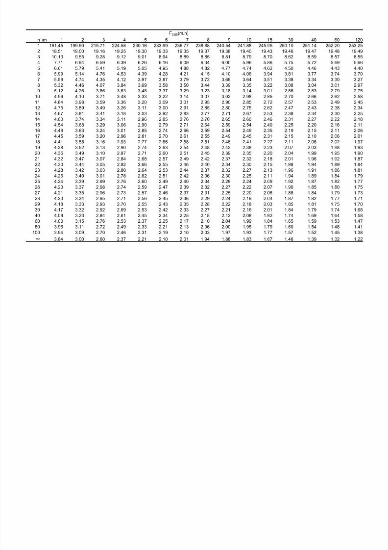
F0.05(m,n)

n \m 1 2 3 4 5 6 7 8 9 10 15 30 40 60 120

1 161.45 199.50 215.71 224.58 230.16 233.99 236.77 238.88 240.54 241.88 245.95 250.10 251.14 252.20 253.25

2 18.51 19.00 19.16 19.25 19.30 19.33 19.35 19.37 19.38 19.40 19.43 19.46 19.47 19.48 19.493 10.13 9.55 9.28 9.12 9.01 8.94 8.89 8.85 8.81 8.79 8.70 8.62 8.59 8.57 8.55

4 7.71 6.94 6.59 6.39 6.26 6.16 6.09 6.04 6.00 5.96 5.86 5.75 5.72 5.69 5.66

5 6.61 5.79 5.41 5.19 5.05 4.95 4.88 4.82 4.77 4.74 4.62 4.50 4.46 4.43 4.40

6 5.99 5.14 4.76 4.53 4.39 4.28 4.21 4.15 4.10 4.06 3.94 3.81 3.77 3.74 3.70

7 5.59 4.74 4.35 4.12 3.97 3.87 3.79 3.73 3.68 3.64 3.51 3.38 3.34 3.30 3.27

8 5.32 4.46 4.07 3.84 3.69 3.58 3.50 3.44 3.39 3.35 3.22 3.08 3.04 3.01 2.97

9 5.12 4.26 3.86 3.63 3.48 3.37 3.29 3.23 3.18 3.14 3.01 2.86 2.83 2.79 2.75

10 4.96 4.10 3.71 3.48 3.33 3.22 3.14 3.07 3.02 2.98 2.85 2.70 2.66 2.62 2.5811 4.84 3.98 3.59 3.36 3.20 3.09 3.01 2.95 2.90 2.85 2.72 2.57 2.53 2.49 2.45

12 4.75 3.89 3.49 3.26 3.11 3.00 2.91 2.85 2.80 2.75 2.62 2.47 2.43 2.38 2.34

13 4.67 3.81 3.41 3.18 3.03 2.92 2.83 2.77 2.71 2.67 2.53 2.38 2.34 2.30 2.25

14 4.60 3.74 3.34 3.11 2.96 2.85 2.76 2.70 2.65 2.60 2.46 2.31 2.27 2.22 2.18

15 4.54 3.68 3.29 3.06 2.90 2.79 2.71 2.64 2.59 2.54 2.40 2.25 2.20 2.16 2.11

16 4.49 3.63 3.24 3.01 2.85 2.74 2.66 2.59 2.54 2.49 2.35 2.19 2.15 2.11 2.06

17 4.45 3.59 3.20 2.96 2.81 2.70 2.61 2.55 2.49 2.45 2.31 2.15 2.10 2.06 2.01

18 4.41 3.55 3.16 2.93 2.77 2.66 2.58 2.51 2.46 2.41 2.27 2.11 2.06 2.02 1.97

19 4.38 3.52 3.13 2.90 2.74 2.63 2.54 2.48 2.42 2.38 2.23 2.07 2.03 1.98 1.93

20 4.35 3.49 3.10 2.87 2.71 2.60 2.51 2.45 2.39 2.35 2.20 2.04 1.99 1.95 1.90

21 4.32 3.47 3.07 2.84 2.68 2.57 2.49 2.42 2.37 2.32 2.18 2.01 1.96 1.92 1.87

22 4.30 3.44 3.05 2.82 2.66 2.55 2.46 2.40 2.34 2.30 2.15 1.98 1.94 1.89 1.84

23 4.28 3.42 3.03 2.80 2.64 2.53 2.44 2.37 2.32 2.27 2.13 1.96 1.91 1.86 1.81

24 4.26 3.40 3.01 2.78 2.62 2.51 2.42 2.36 2.30 2.25 2.11 1.94 1.89 1.84 1.79

25 4.24 3.39 2.99 2.76 2.60 2.49 2.40 2.34 2.28 2.24 2.09 1.92 1.87 1.82 1.77

26 4.23 3.37 2.98 2.74 2.59 2.47 2.39 2.32 2.27 2.22 2.07 1.90 1.85 1.80 1.75

27 4.21 3.35 2.96 2.73 2.57 2.46 2.37 2.31 2.25 2.20 2.06 1.88 1.84 1.79 1.7328 4.20 3.34 2.95 2.71 2.56 2.45 2.36 2.29 2.24 2.19 2.04 1.87 1.82 1.77 1.71

29 4.18 3.33 2.93 2.70 2.55 2.43 2.35 2.28 2.22 2.18 2.03 1.85 1.81 1.75 1.70

30 4.17 3.32 2.92 2.69 2.53 2.42 2.33 2.27 2.21 2.16 2.01 1.84 1.79 1.74 1.68

40 4.08 3.23 2.84 2.61 2.45 2.34 2.25 2.18 2.12 2.08 1.92 1.74 1.69 1.64 1.58

60 4.00 3.15 2.76 2.53 2.37 2.25 2.17 2.10 2.04 1.99 1.84 1.65 1.59 1.53 1.47

80 3.96 3.11 2.72 2.49 2.33 2.21 2.13 2.06 2.00 1.95 1.79 1.60 1.54 1.48 1.41

100 3.94 3.09 2.70 2.46 2.31 2.19 2.10 2.03 1.97 1.93 1.77 1.57 1.52 1.45 1.38

∞

3.84 3.00 2.60 2.37 2.21 2.10 2.01 1.94 1.88 1.83 1.67 1.46 1.39 1.32 1.22



F0.025(m,n)

n \m 1 2 3 4 5 6 7 8 9 10 15 30 40 60 120

1 647.79 799.50 864.16 899.58 921.85 937.11 948.22 956.66 963.28 968.63 984.87 1001.41 1005.60 1009.80 1014.02

2 38.51 39.00 39.17 39.25 39.30 39.33 39.36 39.37 39.39 39.40 39.43 39.46 39.47 39.48 39.493 17.44 16.04 15.44 15.10 14.88 14.73 14.62 14.54 14.47 14.42 14.25 14.08 14.04 13.99 13.95

4 12.22 10.65 9.98 9.60 9.36 9.20 9.07 8.98 8.90 8.84 8.66 8.46 8.41 8.36 8.31

5 10.01 8.43 7.76 7.39 7.15 6.98 6.85 6.76 6.68 6.62 6.43 6.23 6.18 6.12 6.07

6 8.81 7.26 6.60 6.23 5.99 5.82 5.70 5.60 5.52 5.46 5.27 5.07 5.01 4.96 4.90

7 8.07 6.54 5.89 5.52 5.29 5.12 4.99 4.90 4.82 4.76 4.57 4.36 4.31 4.25 4.20

8 7.57 6.06 5.42 5.05 4.82 4.65 4.53 4.43 4.36 4.30 4.10 3.89 3.84 3.78 3.73

9 7.21 5.71 5.08 4.72 4.48 4.32 4.20 4.10 4.03 3.96 3.77 3.56 3.51 3.45 3.39

10 6.94 5.46 4.83 4.47 4.24 4.07 3.95 3.85 3.78 3.72 3.52 3.31 3.26 3.20 3.1411 6.72 5.26 4.63 4.28 4.04 3.88 3.76 3.66 3.59 3.53 3.33 3.12 3.06 3.00 2.94

12 6.55 5.10 4.47 4.12 3.89 3.73 3.61 3.51 3.44 3.37 3.18 2.96 2.91 2.85 2.79

13 6.41 4.97 4.35 4.00 3.77 3.60 3.48 3.39 3.31 3.25 3.05 2.84 2.78 2.72 2.66

14 6.30 4.86 4.24 3.89 3.66 3.50 3.38 3.29 3.21 3.15 2.95 2.73 2.67 2.61 2.55

15 6.20 4.77 4.15 3.80 3.58 3.41 3.29 3.20 3.12 3.06 2.86 2.64 2.59 2.52 2.46

16 6.12 4.69 4.08 3.73 3.50 3.34 3.22 3.12 3.05 2.99 2.79 2.57 2.51 2.45 2.38

17 6.04 4.62 4.01 3.66 3.44 3.28 3.16 3.06 2.98 2.92 2.72 2.50 2.44 2.38 2.32

18 5.98 4.56 3.95 3.61 3.38 3.22 3.10 3.01 2.93 2.87 2.67 2.44 2.38 2.32 2.26

19 5.92 4.51 3.90 3.56 3.33 3.17 3.05 2.96 2.88 2.82 2.62 2.39 2.33 2.27 2.20

20 5.87 4.46 3.86 3.51 3.29 3.13 3.01 2.91 2.84 2.77 2.57 2.35 2.29 2.22 2.16

21 5.83 4.42 3.82 3.48 3.25 3.09 2.97 2.87 2.80 2.73 2.53 2.31 2.25 2.18 2.11

22 5.79 4.38 3.78 3.44 3.22 3.05 2.93 2.84 2.76 2.70 2.50 2.27 2.21 2.14 2.08

23 5.75 4.35 3.75 3.41 3.18 3.02 2.90 2.81 2.73 2.67 2.47 2.24 2.18 2.11 2.04

24 5.72 4.32 3.72 3.38 3.15 2.99 2.87 2.78 2.70 2.64 2.44 2.21 2.15 2.08 2.01

25 5.69 4.29 3.69 3.35 3.13 2.97 2.85 2.75 2.68 2.61 2.41 2.18 2.12 2.05 1.98

26 5.66 4.27 3.67 3.33 3.10 2.94 2.82 2.73 2.65 2.59 2.39 2.16 2.09 2.03 1.95

27 5.63 4.24 3.65 3.31 3.08 2.92 2.80 2.71 2.63 2.57 2.36 2.13 2.07 2.00 1.9328 5.61 4.22 3.63 3.29 3.06 2.90 2.78 2.69 2.61 2.55 2.34 2.11 2.05 1.98 1.91

29 5.59 4.20 3.61 3.27 3.04 2.88 2.76 2.67 2.59 2.53 2.32 2.09 2.03 1.96 1.89

30 5.57 4.18 3.59 3.25 3.03 2.87 2.75 2.65 2.57 2.51 2.31 2.07 2.01 1.94 1.87

40 5.42 4.05 3.46 3.13 2.90 2.74 2.62 2.53 2.45 2.39 2.18 1.94 1.88 1.80 1.72

60 5.29 3.93 3.34 3.01 2.79 2.63 2.51 2.41 2.33 2.27 2.06 1.82 1.74 1.67 1.58

80 5.22 3.86 3.28 2.95 2.73 2.57 2.45 2.35 2.28 2.21 2.00 1.75 1.68 1.60 1.51

100 5.18 3.83 3.25 2.92 2.70 2.54 2.42 2.32 2.24 2.18 1.97 1.71 1.64 1.56 1.46

∞

5.02 3.69 3.13 2.79 2.57 2.41 2.29 2.19 2.11 2.05 1.83 1.57 1.48 1.39 1.27



F0.01(m,n)

n \m 1 2 3 4 5 6 7 8 9 10 15 30 40 60 120

1 4052 4999 5403 5625 5764 5859 5928 5981 6022 6056 6157 6261 6287 6313 6339

2 98.5 99.0 99.2 99.2 99.3 99.3 99.4 99.4 99.4 99.4 99.4 99.5 99.5 99.5 99.53 34.1 30.8 29.5 28.7 28.2 27.9 27.7 27.5 27.3 27.2 26.9 26.5 26.4 26.3 26.2

4 21.2 18.0 16.7 16.0 15.5 15.2 15.0 14.8 14.7 14.5 14.2 13.8 13.7 13.7 13.6

5 16.3 13.3 12.1 11.4 11.0 10.7 10.5 10.3 10.2 10.1 9.72 9.38 9.29 9.20 9.11

6 13.75 10.92 9.78 9.15 8.75 8.47 8.26 8.10 7.98 7.87 7.56 7.23 7.14 7.06 6.97

7 12.25 9.55 8.45 7.85 7.46 7.19 6.99 6.84 6.72 6.62 6.31 5.99 5.91 5.82 5.74

8 11.26 8.65 7.59 7.01 6.63 6.37 6.18 6.03 5.91 5.81 5.52 5.20 5.12 5.03 4.95

9 10.56 8.02 6.99 6.42 6.06 5.80 5.61 5.47 5.35 5.26 4.96 4.65 4.57 4.48 4.40

10 10.04 7.56 6.55 5.99 5.64 5.39 5.20 5.06 4.94 4.85 4.56 4.25 4.17 4.08 4.0011 9.65 7.21 6.22 5.67 5.32 5.07 4.89 4.74 4.63 4.54 4.25 3.94 3.86 3.78 3.69

12 9.33 6.93 5.95 5.41 5.06 4.82 4.64 4.50 4.39 4.30 4.01 3.70 3.62 3.54 3.45

13 9.07 6.70 5.74 5.21 4.86 4.62 4.44 4.30 4.19 4.10 3.82 3.51 3.43 3.34 3.25

14 8.86 6.51 5.56 5.04 4.69 4.46 4.28 4.14 4.03 3.94 3.66 3.35 3.27 3.18 3.09

15 8.68 6.36 5.42 4.89 4.56 4.32 4.14 4.00 3.89 3.80 3.52 3.21 3.13 3.05 2.96

16 8.53 6.23 5.29 4.77 4.44 4.20 4.03 3.89 3.78 3.69 3.41 3.10 3.02 2.93 2.84

17 8.40 6.11 5.18 4.67 4.34 4.10 3.93 3.79 3.68 3.59 3.31 3.00 2.92 2.83 2.75

18 8.29 6.01 5.09 4.58 4.25 4.01 3.84 3.71 3.60 3.51 3.23 2.92 2.84 2.75 2.66

19 8.18 5.93 5.01 4.50 4.17 3.94 3.77 3.63 3.52 3.43 3.15 2.84 2.76 2.67 2.58

20 8.10 5.85 4.94 4.43 4.10 3.87 3.70 3.56 3.46 3.37 3.09 2.78 2.69 2.61 2.52

21 8.02 5.78 4.87 4.37 4.04 3.81 3.64 3.51 3.40 3.31 3.03 2.72 2.64 2.55 2.46

22 7.95 5.72 4.82 4.31 3.99 3.76 3.59 3.45 3.35 3.26 2.98 2.67 2.58 2.50 2.40

23 7.88 5.66 4.76 4.26 3.94 3.71 3.54 3.41 3.30 3.21 2.93 2.62 2.54 2.45 2.35

24 7.82 5.61 4.72 4.22 3.90 3.67 3.50 3.36 3.26 3.17 2.89 2.58 2.49 2.40 2.31

25 7.77 5.57 4.68 4.18 3.85 3.63 3.46 3.32 3.22 3.13 2.85 2.54 2.45 2.36 2.27

26 7.72 5.53 4.64 4.14 3.82 3.59 3.42 3.29 3.18 3.09 2.81 2.50 2.42 2.33 2.23

27 7.68 5.49 4.60 4.11 3.78 3.56 3.39 3.26 3.15 3.06 2.78 2.47 2.38 2.29 2.2028 7.64 5.45 4.57 4.07 3.75 3.53 3.36 3.23 3.12 3.03 2.75 2.44 2.35 2.26 2.17

29 7.60 5.42 4.54 4.04 3.73 3.50 3.33 3.20 3.09 3.00 2.73 2.41 2.33 2.23 2.14

30 7.56 5.39 4.51 4.02 3.70 3.47 3.30 3.17 3.07 2.98 2.70 2.39 2.30 2.21 2.11

40 7.31 5.18 4.31 3.83 3.51 3.29 3.12 2.99 2.89 2.80 2.52 2.20 2.11 2.02 1.92

60 7.08 4.98 4.13 3.65 3.34 3.12 2.95 2.82 2.72 2.63 2.35 2.03 1.94 1.84 1.73

80 6.96 4.88 4.04 3.56 3.26 3.04 2.87 2.74 2.64 2.55 2.27 1.94 1.85 1.75 1.63

100 6.90 4.82 3.98 3.51 3.21 2.99 2.82 2.69 2.59 2.50 2.22 1.89 1.80 1.69 1.57

∞

6.63 4.61 3.78 3.32 3.02 2.80 2.64 2.51 2.41 2.32 2.04 1.70 1.59 1.47 1.32

Documents

Stats Formulas &Tables