Embed Size (px)
Citation preview
Graphs and edgelists567 Social network analysis
Peter Hoff
Statistics, University of Washington
1/28
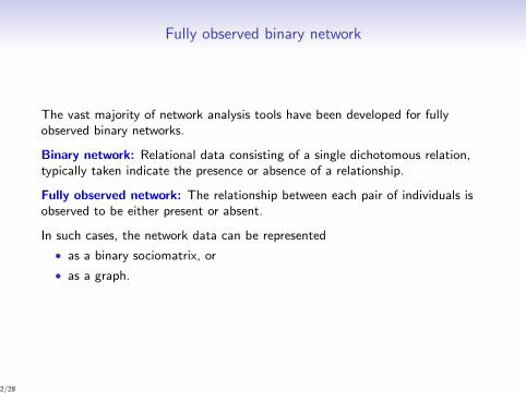
Fully observed binary network
The vast majority of network analysis tools have been developed for fullyobserved binary networks.
Binary network: Relational data consisting of a single dichotomous relation,typically taken indicate the presence or absence of a relationship.
Fully observed network: The relationship between each pair of individuals isobserved to be either present or absent.
In such cases, the network data can be represented
• as a binary sociomatrix, or
• as a graph.
2/28
Nodes and edges
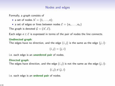
Formally, a graph consists of
• a set of nodes N = {1, . . . , n};• a set of edges or lines between nodes E = {e1, . . . , em}
The graph is denoted G = (N , E).
Each edge e ∈ E is expressed in terms of the pair of nodes the line connects.
Undirected graph:The edges have no direction, and the edge {i , j} is the same as the edge {j , i}:
{i , j} = {j , i}
i.e. each edge is an unordered pair of nodes.
Directed graph:The edges have direction, and the edge (i , j) is not the same as the edge (j , i):
(i , j) 6= (j , i)
i.e. each edge is an ordered pair of nodes.
3/28
Example of an undirected graph
N = {1, 2, 3, 4, 5}E = {{1, 2}, {1, 3}, {2, 3}, {2, 4}, {2, 5}, {3, 5}, {4, 5}}
Exercise: Draw this graph
4/28
Example of a directed graph
N = {1, 2, 3, 4, 5}E = {(1, 3), (2, 3), (2, 4), (2, 5), (3, 1), (3, 5), (4, 5), (5, 4)}
Exercise: Draw this graph
5/28
Some graph terminology
For an undirected graph G = {N , E}• adjacent : nodes i and j are adjacent if {i , j} ∈ E• incident : node i is incident with edge e if e = {i , j} for some j ∈ N .
• empty : the graph is empty if E = ∅, i.e. there are no edges.
• complete : the graph is complete if
E = {{i , j} : i ∈ N , j ∈ N , i 6= j},
that is, all possible edges are present.
Similar definitions are used for directed graphs.
Exercise: Identify some adjacent nodes and incident node-edge pairs for theprevious two example graphs.
6/28
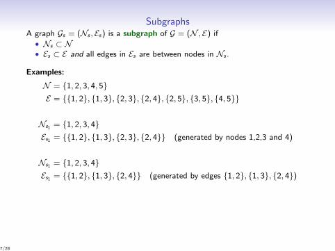
SubgraphsA graph Gs = (Ns , Es) is a subgraph of G = (N , E) if
• Ns ⊂ N• Es ⊂ E and all edges in Es are between nodes in Ns .
Examples:
N = {1, 2, 3, 4, 5}E = {{1, 2}, {1, 3}, {2, 3}, {2, 4}, {2, 5}, {3, 5}, {4, 5}}
Ns1 = {1, 2, 3, 4}Es1 = {{1, 2}, {1, 3}, {2, 3}, {2, 4}} (generated by nodes 1,2,3 and 4)
Ns1 = {1, 2, 3, 4}Es1 = {{1, 2}, {1, 3}, {2, 4}} (generated by edges {1, 2}, {1, 3}, {2, 4})
7/28
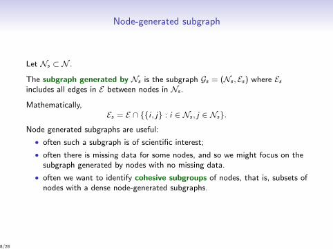
Node-generated subgraph
Let Ns ⊂ N .
The subgraph generated by Ns is the subgraph Gs = (Ns , Es) where Esincludes all edges in E between nodes in Ns .
Mathematically,Es = E ∩ {{i , j} : i ∈ Ns , j ∈ Ns}.
Node generated subgraphs are useful:
• often such a subgraph is of scientific interest;
• often there is missing data for some nodes, and so we might focus on thesubgraph generated by nodes with no missing data.
• often we want to identify cohesive subgroups of nodes, that is, subsets ofnodes with a dense node-generated subgraphs.
8/28
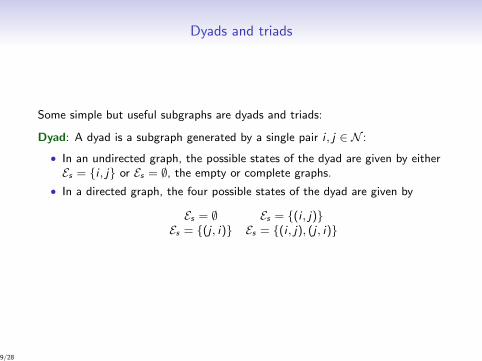
Dyads and triads
Some simple but useful subgraphs are dyads and triads:
Dyad: A dyad is a subgraph generated by a single pair i , j ∈ N :
• In an undirected graph, the possible states of the dyad are given by eitherEs = {i , j} or Es = ∅, the empty or complete graphs.
• In a directed graph, the four possible states of the dyad are given by
Es = ∅ Es = {(i , j)}Es = {(j , i)} Es = {(i , j), (j , i)}
9/28
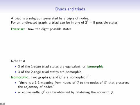
Dyads and triads
A triad is a subgraph generated by a triple of nodes.For an undirected graph, a triad can be in one of 23 = 8 possible states.
Exercise: Draw the eight possible states.
Note that
• 3 of the 1-edge triad states are equivalent, or isomorphic,
• 3 of the 2-edge triad states are isomorphic.
Isomorphic: Two graphs G and G′ are isomorphic if
• “there is a 1-1 mapping from nodes of G to the nodes of G′ that preservesthe adjacency of nodes.”
• or equivalently, G′ can be obtained by relabeling the nodes of G.
10/28
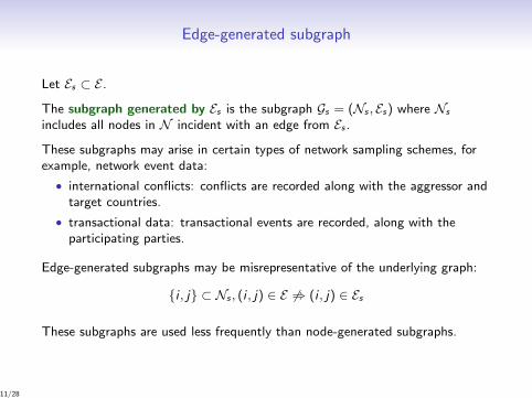
Edge-generated subgraph
Let Es ⊂ E .
The subgraph generated by Es is the subgraph Gs = (Ns , Es) where Ns
includes all nodes in N incident with an edge from Es .
These subgraphs may arise in certain types of network sampling schemes, forexample, network event data:
• international conflicts: conflicts are recorded along with the aggressor andtarget countries.
• transactional data: transactional events are recorded, along with theparticipating parties.
Edge-generated subgraphs may be misrepresentative of the underlying graph:
{i , j} ⊂ Ns , (i , j) ∈ E 6⇒ (i , j) ∈ Es
These subgraphs are used less frequently than node-generated subgraphs.
11/28
Edge lists
Graphs are often stored on a computer in terms of their edge set, or edge list.
The edge list completely represents the graph unless there are isolated nodes:
Isolated node or isolate: A node that is not adjacent to any other node.
Examples:
In the presence of isolates, the graph can be represented with the edge list anda list of isolates.
12/28
Graph-theoretic terms
• graph, node set, edge set, edge list
• undirected graph, directed graph
• adjacent, incident, empty, complete
• subgraph, generated subgraph, dyad, triad
• isomorphic
• isolate
13/28
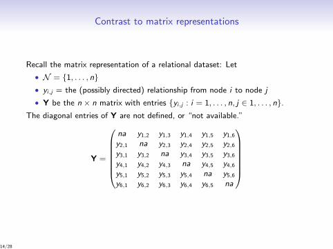
Contrast to matrix representations
Recall the matrix representation of a relational dataset: Let
• N = {1, . . . , n}• yi,j = the (possibly directed) relationship from node i to node j
• Y be the n × n matrix with entries {yi,j : i = 1, . . . , n, j ∈ 1, . . . , n}.The diagonal entries of Y are not defined, or “not available.”
Y =
na y1,2 y1,3 y1,4 y1,5 y1,6y2,1 na y2,3 y2,4 y2,5 y2,6y3,1 y3,2 na y3,4 y3,5 y3,6y4,1 y4,2 y4,3 na y4,5 y4,6y5,1 y5,2 y5,3 y5,4 na y5,6y6,1 y6,2 y6,3 y6,4 y6,5 na
14/28
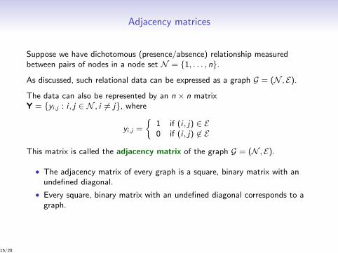
Adjacency matrices
Suppose we have dichotomous (presence/absence) relationship measuredbetween pairs of nodes in a node set N = {1, . . . , n}.
As discussed, such relational data can be expressed as a graph G = (N , E).
The data can also be represented by an n × n matrixY = {yi,j : i , j ∈ N , i 6= j}, where
yi,j =
{1 if (i , j) ∈ E0 if (i , j) 6∈ E
This matrix is called the adjacency matrix of the graph G = (N , E).
• The adjacency matrix of every graph is a square, binary matrix with anundefined diagonal.
• Every square, binary matrix with an undefined diagonal corresponds to agraph.
15/28
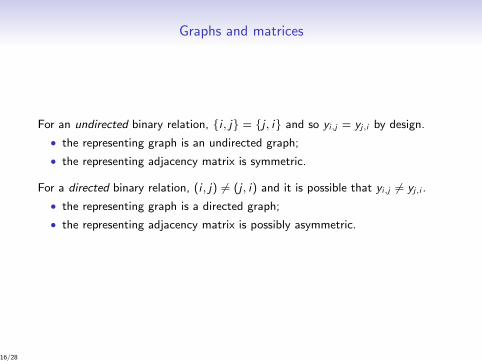
Graphs and matrices
For an undirected binary relation, {i , j} = {j , i} and so yi,j = yj,i by design.
• the representing graph is an undirected graph;
• the representing adjacency matrix is symmetric.
For a directed binary relation, (i , j) 6= (j , i) and it is possible that yi,j 6= yj,i .
• the representing graph is a directed graph;
• the representing adjacency matrix is possibly asymmetric.
16/28

Adjacency matrices
Exercise: Draw the directed graph represented by the following matrix:
Y =
na 0 1 1 0 11 na 1 0 0 10 0 na 1 0 10 0 1 na 0 11 0 1 1 na 10 0 1 1 0 na
17/28
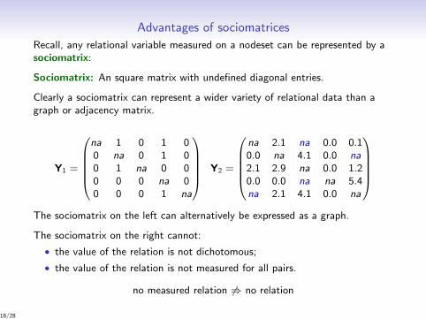
Advantages of sociomatrices
Recall, any relational variable measured on a nodeset can be represented by asociomatrix:
Sociomatrix: An square matrix with undefined diagonal entries.
Clearly a sociomatrix can represent a wider variety of relational data than agraph or adjacency matrix.
Y1 =
na 1 0 1 00 na 0 1 00 1 na 0 00 0 0 na 00 0 0 1 na
Y2 =
na 2.1 na 0.0 0.10.0 na 4.1 0.0 na2.1 2.9 na 0.0 1.20.0 0.0 na na 5.4na 2.1 4.1 0.0 na
The sociomatrix on the left can alternatively be expressed as a graph.
The sociomatrix on the right cannot:
• the value of the relation is not dichotomous;
• the value of the relation is not measured for all pairs.
no measured relation 6⇒ no relation
18/28
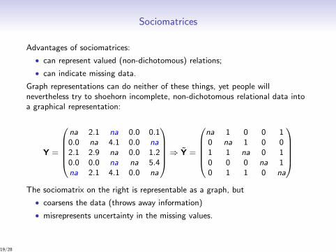
Sociomatrices
Advantages of sociomatrices:
• can represent valued (non-dichotomous) relations;
• can indicate missing data.
Graph representations can do neither of these things, yet people willnevertheless try to shoehorn incomplete, non-dichotomous relational data intoa graphical representation:
Y =
na 2.1 na 0.0 0.10.0 na 4.1 0.0 na2.1 2.9 na 0.0 1.20.0 0.0 na na 5.4na 2.1 4.1 0.0 na
⇒ Y =
na 1 0 0 10 na 1 0 01 1 na 0 10 0 0 na 10 1 1 0 na
The sociomatrix on the right is representable as a graph, but
• coarsens the data (throws away information)
• misrepresents uncertainty in the missing values.
19/28
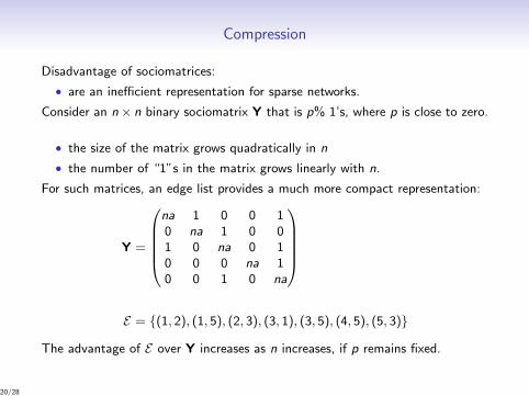
Compression
Disadvantage of sociomatrices:
• are an inefficient representation for sparse networks.
Consider an n× n binary sociomatrix Y that is p% 1’s, where p is close to zero.
• the size of the matrix grows quadratically in n
• the number of “1”s in the matrix grows linearly with n.
For such matrices, an edge list provides a much more compact representation:
Y =
na 1 0 0 10 na 1 0 01 0 na 0 10 0 0 na 10 0 1 0 na
E = {(1, 2), (1, 5), (2, 3), (3, 1), (3, 5), (4, 5), (5, 3)}
The advantage of E over Y increases as n increases, if p remains fixed.
20/28
Weighted edges
Often the relational variable is either zero or some arbitrary non-zero value.
• communication networks:
yi,j = number of emails sent from i to j
yi,j ∈ {0, 1, 2, . . .}
• conflict networks:
yi,j = military relationship between i and j
yi,j ∈ {−1, 0, 1}
In both cases, yi,j = 0 for the vast majority of i , j-pairs.In such cases, a weighted edge list can be more efficient than a sociomatrix.
21/28
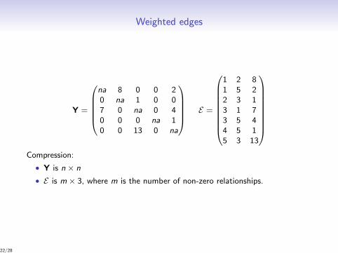
Weighted edges
Y =
na 8 0 0 20 na 1 0 07 0 na 0 40 0 0 na 10 0 13 0 na
E =
1 2 81 5 22 3 13 1 73 5 44 5 15 3 13
Compression:
• Y is n × n
• E is m × 3, where m is the number of non-zero relationships.
22/28
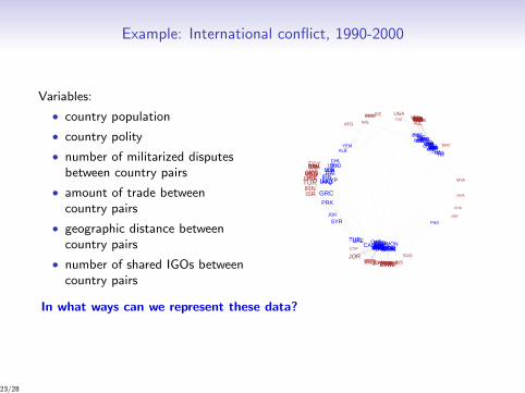
Example: International conflict, 1990-2000
Variables:
• country population
• country polity
• number of militarized disputesbetween country pairs
• amount of trade betweencountry pairs
• geographic distance betweencountry pairs
• number of shared IGOs betweencountry pairs
AFGANG
ARG
AUL
BAH
BNGBOTBUI
CAN
CAO
CHA
CHN
COS
CUB
CYP
DOM
DRC
EGY
FRN
GHA
GRC
GUI HON
IND INS
IRN
IRQ
ISR
ITA
JORJPN
KENLBRLESLIBMAL
MYA
NICNIG NIR
NTHOMA
PAK
PHIPRK
QAT
ROK
RWASAFSAL
SAU
SENSIE
SRI
SUD
SWA
SYRTAW
TAZTHITOG
TUR
UAE
UGA
UKGUSA
VEN
AFG
ALB
ANG
ARGAULBAHBEL
BEN
BNG
BUICAM
CAN
CDICHA
CHL
CHN
COL
CONCOS
CUB
CYP
DRC
EGYFRN
GHAGNB
GRC
GUIGUY
HAI
HONIND
INS
IRNIRQ
ISRITA
JOR
JPN
LBR
LES
LIB
MAAMLI
MONMOR
MYAMZM
NAMNICNIG
NIRNTHOMAPAK PHI
PNG
PRK
QATROK
RWA
SAFSAL
SAUSENSIE
SIN
SPN
SUD
SYR
TAW
TAZ
THITOG
TRI
TURUAE
UGA
UKGUSA
VEN
YEMZAM
ZIM
In what ways can we represent these data?
23/28
Example: International conflict, 1990-2000
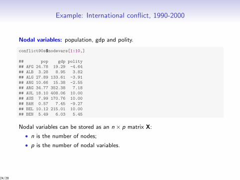
Nodal variables: population, gdp and polity.
conflict90s$nodevars[1:10,]
## pop gdp polity## AFG 24.78 19.29 -4.64## ALB 3.28 8.95 3.82## ALG 27.89 133.61 -3.91## ANG 10.66 15.38 -2.55## ARG 34.77 352.38 7.18## AUL 18.10 408.06 10.00## AUS 7.99 170.76 10.00## BAH 0.57 7.45 -9.27## BEL 10.12 215.01 10.00## BEN 5.49 6.03 5.45
Nodal variables can be stored as an n × p matrix X:
• n is the number of nodes;
• p is the number of nodal variables.
24/28
Example: International conflict, 1990-2000
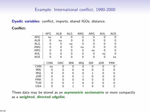
Dyadic variables: conflict, imports, shared IGOs, distance.
Conflict:
AFG ALB ALG ANG ARG AUL AUSAFG na 0 0 0 0 0 0ALB 0 na 0 0 0 0 0ALG 0 0 na 0 0 0 0ANG 0 0 0 na 0 0 0ARG 0 0 0 0 na 0 0AUL 0 0 0 0 0 na 0AUS 0 0 0 0 0 0 na
CHN DRC IRN IRQ ISR JOR PRKCHN na 0 0 0 0 0 0IRN 0 0 0 6 0 0 0IRQ 0 0 0 0 1 0 0JOR 0 0 0 1 0 0 0PRK 3 0 0 0 0 0 0TUR 0 0 2 6 0 0 0USA 0 0 1 7 0 0 2
These data may be stored as an asymmetric sociomatrix or more compactlyas a weighted, directed edgelist.
25/28
Example: International conflict, 1990-2000
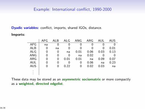
Dyadic variables: conflict, imports, shared IGOs, distance.
Imports:
AFG ALB ALG ANG ARG AUL AUSAFG na 0 0 0 0 0 0ALB 0 na 0 0 0 0 0.01ALG 0 0 na 0.01 0.06 0.03 0.13ANG 0 0 0 na 0.02 0 0ARG 0 0 0.01 0.01 na 0.09 0.07AUL 0 0 0 0 0.06 na 0.23AUS 0 0 0.22 0 0.02 0.03 na...
These data may be stored as an asymmetric sociomatrix or more compactlyas a weighted, directed edgelist.
26/28
Example: International conflict, 1990-2000
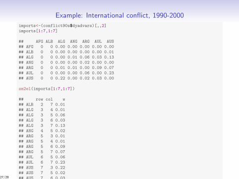
imports<-(conflict90s$dyadvars)[,,2]imports[1:7,1:7]
## AFG ALB ALG ANG ARG AUL AUS## AFG 0 0 0.00 0.00 0.00 0.00 0.00## ALB 0 0 0.00 0.00 0.00 0.00 0.01## ALG 0 0 0.00 0.01 0.06 0.03 0.13## ANG 0 0 0.00 0.00 0.02 0.00 0.00## ARG 0 0 0.01 0.01 0.00 0.09 0.07## AUL 0 0 0.00 0.00 0.06 0.00 0.23## AUS 0 0 0.22 0.00 0.02 0.03 0.00
sm2el(imports[1:7,1:7])
## row col w## ALB 2 7 0.01## ALG 3 4 0.01## ALG 3 5 0.06## ALG 3 6 0.03## ALG 3 7 0.13## ANG 4 5 0.02## ARG 5 3 0.01## ARG 5 4 0.01## ARG 5 6 0.09## ARG 5 7 0.07## AUL 6 5 0.06## AUL 6 7 0.23## AUS 7 3 0.22## AUS 7 5 0.02## AUS 7 6 0.0327/28
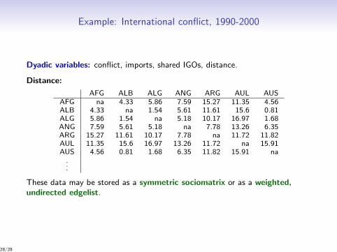
Example: International conflict, 1990-2000
Dyadic variables: conflict, imports, shared IGOs, distance.
Distance:
AFG ALB ALG ANG ARG AUL AUSAFG na 4.33 5.86 7.59 15.27 11.35 4.56ALB 4.33 na 1.54 5.61 11.61 15.6 0.81ALG 5.86 1.54 na 5.18 10.17 16.97 1.68ANG 7.59 5.61 5.18 na 7.78 13.26 6.35ARG 15.27 11.61 10.17 7.78 na 11.72 11.82AUL 11.35 15.6 16.97 13.26 11.72 na 15.91AUS 4.56 0.81 1.68 6.35 11.82 15.91 na...
These data may be stored as a symmetric sociomatrix or as a weighted,undirected edgelist.
28/28