Statistics 580

Introduction to Markov Chain Monte Carlo

Introduction to Markov Chains

A stochastic process is a sequence of random variables {X(t), t ∈ T} indexed by a parameter t inan index set T. X(t) is called the state of the process at time t and the set of possible realizations ofX(t) defines the state space denoted by S. The time or the parameter space may be discrete, for e.g.,T = {0, 1, . . .} or continuous, for e.g., T = (0, ∞). The state space may also be discrete, for e.g.,S = {0, 1, . . .} or continuous, for e.g., S = (−∞, ∞).

A discrete parameter stochastic process {X(t), t = 0, 1, 2. . . .} or a continuous parameter process{X(t), t ≥ 0} is said to be a Markov process if, for any set of n time points t1 < t2 < . . . < tn inthe index set T ,

Pr[X(tn) ≤ xn|X(tn−1) = xn−1, . . . , X(t1) = x1] = Pr[X(tn) ≤ xn|X(tn−1) = xn−1].

It says that the probability distribution of future states in a Markov process depends only on the present(or most recently observed) state and not on the past states. Markov processes are classified accordingto the nature of the state space or the parameter space. A Markov process whose state space is discreteis called a Markov chain. We shall use the set {0, 1, . . .} to denote the state space of a Markov chainand first consider discrete parameter Markov chains where, without loss of generality, we shall usethe notation X0, X1, . . . , Xn, . . . to denote the states.

The transition probability function of a discrete parameter Markov chain that define the proba-bility distribution of the next state given the present state is given by,

pij(m,n) = Pr(Xn = j|Xm = i)

for all states i and j and n ≥ m. The matrix of transition probabilities is denoted by P (m,n) =(pij(m,n)). In order to give the probability law of a discrete parameter Markov chain {Xn} it is sufficientto specify, for all times n ≥ m, pj(n) = P (Xn = j) and pij(m,n) for all states i and j. A fundamentalrelation satisfied by the transition probability function of a Markov chain is the Chapman-Kolmogorov

equation: for any times n > u > m and states i and j,

pij(m,n) =∑

k

pik(m,u)pkj(u, n).

or, in terms of transition probability matrices,

P (m,n) = P (m,u) P (u, n).

If pij(m,n) depend only on the difference n − m they are said to be stationary transition

probabilities and the Markov chain is said to be stationary or homogeneous. In a stationary Markovchain, the k-step transition probability function is denoted by

p(k)ij = Pr(Xn+k = j|Xn = i)

1

and the k-step transition probability matrix by P (k), where P (k) = (p(k)ij ). The one-step transition

probabilities of a stationary Markov chain are denoted by

p(1)ij ≡ pij = Pr(Xn = j|Xn−1 = i)

where by definition∑

j

pij = 1 and the matrix of these transition probabilities is the square matrix

P =

p11 p12 p13 · · ·p21 p22 p23 · · ·...

...... · · ·

,

and is called the one-step transition matrix. We see that the rows of P sum to one and hence itis a stochastic matrix or a marix of probabilities. As an example, in image analysis a binary image isrepresented in pixels where black or white pixels are indicated by θi = 1 or 0, respectively. The posteriorjoint density of the true image θ given the observed noisy image x (i.e., observed data) is

p(θ|x) ∝ f(x|θ)g(θ)

where f(x|θ) is the model for how the true image is corrupted by noise, and g(θ) is the prior that involvesknowledge about the types of images under consideration. The number of rows (= number of columns)of P in this example may be 2262,144 > 107,857.

Examples of discrete parameter Markov chains:

Example 1 - Two-state Markov chains:A two-state weather model with the two states being “rain” or “no rain”, on successive days. The one-steptransition probability matrix is:

P = rainno rain

rain(

αβ

no rain1 − α1 − β

)

where the elements represent probabilities that it will rain or not on given day conditional on that it rainedor not the previous day. Here the Markov chain will be homogeneous since the transition probabilitiesare stationary, since they are unaffected by what day it is.

Example 2:

Toss a coin where Pr(head) = p, repeatedly. After the nth toss, let Xn represent the number of headsthat have appeared so far.

Then the one-step transition probability matrix is:

P =

1 − p p 0 . . . . . . 00 1 − p p . . . . . . 00 0 1 − p p . . . 0...

......

... . . . 0

where the elements of the 1st row are

p11 = P (Xn = 1 | Xn−1 = 1) ,p12 = P (Xn = 2 | Xn−1 = 1) ,p13 = P (Xn = 3 | Xn−1 = 1) , ..., etc.

2

and the elements of the 2nd row are

p21 = P (Xn = 1 | Xn−1 = 2) ,p22 = P (Xn = 2 | Xn−1 = 2) ,p23 = P (Xn = 3 | Xn−1 = 2) ,p24 = P (Xn = 4 | Xn−1 = 2) , ..., etc.

We see that Xn = Xn−1 + S where S ∼ Bernoulli and Xn−1 and S are independent, which implies that{Xn} is a Markov chain.

Some definitions and results about discrete parameter Markov chains

Recall that the k-step transition probability function was defined as

p(k)ij = Pr(Xn+k = j |Xn = i)

for any integer n. The notationXn+k = j |Xn = i

says that X goes from state i to state j in k steps in time. P (k) denotes the k-step transition matrix,whose elements are p

(k)ij , and P is the one-step transition matrix whose elements are pij. For a stationary

Markov chain

P (k) = P k

p(k) = p(0) P k

where

p(k) =

p(k)1

p(k)2...

p(k)j...

, p(0) =

p1

p2...pj...

, p(k)j = Pr(Xn+k = j), and, pj = Pr(Xn = j),

are the k-step unconditional probabilities. Note that p(0)j ≡ pj is the pmf of the random variable Xn, p

(1)j

is the pmf of the random variable Xn+1, etc. These results are immediate from the Chapman-Kolmogorovequations. Consequently, the probability law of a homogeneous Markov chains is completely determinedonce one knows the one-step transition probability matrix P and the unconditional probability vectorp(0) at time 0.

Example:The two-state weather model with α = 0.7, β = 0.4 is stationary. Thus it follows that

P =

(

0.7 0.30.4 0.6

)

P 2 =

(

0.61 0.390.52 0.48

)

P 4 =

(

0.575 0.4250.567 0.433

)

Note that the rows of P 4 are almost identical showing that the probability of rain or no rain on a certainday does not depend on whether it rained or not four days earlier.

3

Some properties of Markov chains:

The following definitions, properties and results are useful, in general, and for defining certain usefulclasses of Markov chains, in particular:

1. Markov chain is irreducible if every state can be reached from every other state. That is, for alli, j there exists some k0 such that p

(k0)ij > 0. We say that all states communicate with each other.

Example: The chain described by P on the left is irreducible and the chain described by P on theright is not:

P =

0.5 0.5 0.00.5 0.3 0.20.0 0.3 0.7

P =

0.5 0.5 0.0 0.00.5 0.5 0.0 0.00.2 0.3 0.3 0.20.0 0.0 0.0 1.0

2. Define f(k)ij ≡ Pr(Xn+k = j for the 1st time |Xn = i). That is, f

(k)ij is the probabilty that Xn+k is

for the first time in the jth state given that Xn was in the ith state. Thus f(k)jj probability of first

passage from state j to state j in k-steps. The jth state is said to be persistent (i.e.,not transient) if

∞∑

k=1

f(k)jj = 1.

That is, having started at state j, the probability that the chain will eventually return to j is one.Note that in the literature the term recurrent is sometimes used in place of the term persistent todescribe states that satisfy this condition.

3. The jth state is periodic of period tj if p(k)jj > 0 only when k = ν tj where ν is an integer.

4. Markov chain is aperiodic if no states are periodic.

5. The Markov chain is persistent (not transient) if all states are not transient.

TheoremConsider an irreducible, aperiodic, and persistent Markov chain whose mean recurrence time is finite,i.e.,

mjj =∞∑

k=1

k f(k)jj < ∞ .

An invariant (or limiting) distribution for the Markov chain is said to exist if there exists a probabilitydistribution {πj} such that,

limk→∞

p(k)ij = πj

for all j = 1, 2, . . .. If the invariant distribution {πj} exists then it is the unique solution to the equation

πj =∑

i

πi pij. (1)

that satisfies∑

πj = 1.

4

Equation (1) follows since

P k =(

p(k)ij

)k→∞−→

π1 π2 · · ·...π1 π2

and clearly, P k+1 = P k P . Therefore, as k → ∞,

π′

π′

...π′

=

π′

...

...π′

P ,

where π′ = (π1, π2, . . . , ), which implies (1). P is said to satisfy global balance if pij satisfies (1). π is alsoknown as the equilibrium distribution or the stationary distribution.

The idea behind Markov chain Monte Carlo is to find an appropriate Markov chain (i.e, P ) whoseinvariant distribution {πj} is the distribution from which we wish to draw samples. From a startingrealization X0, simulate X1 according to the transition matrix P subsequently simulate X2 from X1 andP and so forth. After a burn in

p(k)ij = Pr

(

Xk = j|X0 = i)

' πj

and so Xk is a realization from the distribution {πj, j = 1, 2, . . .}. How can we find such a Markov chain?We need at least one more result.

Reversibility of Markov chains

Let {Xn : −∞ < n < ∞} be a Markov chain with invariant distribution {πj}. Then Pr(Xn = j) = πj.Consider the time-reversed process

Zn = X−n

Now {Zn} is a Markov chain with transition probabilities

qij = Pr(Zn = j|Zn−1 = i)

= Pr(Zn = j , Zn−1 = i)/Pr(Xn−1 = i)

= Pr(X−n+1 = i|X−n = j)Pr(X−n = j)

P (X−n+1 = i)

= pjiπj

πi

The Markov chain is time reversible if {Zn}d= {Xn} which implies qij = pij which in turn implies

πj pji = πi pij (2)

for all i, j ∈ S.

5

Proposition

Equation (2) implies Equation (1).

Proof:

R.H.S. of (1) =∑

i

πi pij

=∑

i

πj pji

= πj = L.H.S. of (1) .

Condition (2) is obviously the stronger condition and the π are said to satisfy detailed balance. To simulatesamples from a distribution {πj}, it is sufficient that a Markov chain is defined via transition probabilities{pij} that satisfy the relation πi pij = πj pji . This relation is called the reversibility condition. MarkovChain Monte Carlo turns the theory around: the invariant density is known (perhaps up to a constantmultiple) – actually it is the target density from which samples are desired – but the transition matrix isunknown. To generate samples from π(.), Markov Chain Monte Carlo methods use a transition matrixcalled a nominating matrix and employs an acceptance-rejection algorithm whose nth iterate convergesto π(.) for large n.

Metropolis algorithm (Metropolis, et al., 1953)

Suppose the nominating matrix Q is any symmetric matrix of probabilities i.e., qij = qji. We would liketo obtain a sample from a distribution {πj} where πj = Pr(Xn = j) by generating observations from aMarkov chain that has {πj} as its invariant distribution. Metropolis algorithm starts with proposed statei and decides whether it moves to a new state j based on Bernoulli trial:

Step

0. Set xn−1 = i where i is any realization from πi.

1. Generate j from the probability distribution {qij; j = 1, 2, . . .}

2. Set r = πj/πi.

3. If r ≥ 1 set xn = jOtherwise generate u from U(0, 1)if u < r set xn = jelse set xn = xn−1

4. Set n = n + 1, go to Step 1 .

In the above algorithm, the value j is accepted with probability αij = min {πj/πi, 1}. The proof that theequilibrium distribution of the chain constructed by the above algorithm is indeed {πj}, it is sufficient tocheck that the detailed balance condition holds.

6

Example: As an application of the Metropolis algorithm, suppose that we want to generate from thePoisson distribution with mean λ i.e.,

πj = P(

Xn = j)

=1

j!λj e−λ, j = 0, 1, . . .

We will use the nominating probability matrix

Q =

1/2 1/2 0 0 · · ·1/2 0 1/2 0 0 · · ·0 1/2 0 1/2 0 · · ·0 0 1/2 0 1/2 · · ·...

......

......

i.e.,

q00 = 1/2

qij = 1/2 for j = i − 1

= 1/2 for j = i + 1

= 0, otherwise

which is symmetric (and is a one-step transition matrix).

The Metropolis algorithm for generating samples from Poisson(6) is as follows:

Step 0. Start with xn−1 = i

Step 1. Generate j from {qij}

if i 6= 0

i.e. , generate u1 from U(0, 1)

if u1 < 1/2, set j = i − 1

else set j = i + 1

if i = 0

{

if u1 < 1/2, set j = 0

else set j = 1

Step 2. Set r = πj/πi = (i! λj)(j! λi)

i.e., set r = 1, if i = 0, j = 0

= i/λ, if j = i − 1

= λ/j, if j = i + 1

Step 3. If r ≥ 1, set xn = j

Otherwise, generate u2 from U(0, 1)

if u2 < r, set xn = j

else, set xn = xn−1

Step 4. Set n = n + 1, go to 1

7

The table below display values of relevant quantities computed in the first 15 iterations of this algo-rithm for Poisson with λ = 6 starting with x0 = 2:

--------------------------------------------------

n i u1 j r u2

---------------------------------------------------

1 2 0.71889082 3 2.0000000 0.83568994

2 3 0.92144722 4 1.5000000 0.67244221

3 4 0.48347869 3 0.6666667 0.23677552

4 3 0.38764000 2 0.5000000 0.70580029

5 3 0.66973964 4 1.5000000 0.47446056

6 4 0.51325076 5 1.2000000 0.44375696

7 5 0.22118260 4 0.8333333 0.79923561

8 4 0.32724500 3 0.6666667 0.55147710

9 3 0.32624403 2 0.5000000 0.88511680

10 3 0.32752058 2 0.5000000 0.82785282

11 3 0.51644296 4 1.5000000 0.30783601

12 4 0.53919790 5 1.2000000 0.40234452

13 5 0.95002276 6 1.0000000 0.07881027

14 6 0.07521049 5 1.0000000 0.25551719

15 5 0.78899123 6 1.0000000 0.59512748

---------------------------------------------------

The R code that was used to generate these iterates is as follows:

poisson.metro=function(lamda,i,n)

{

y=seq(n)

for(k in 1:n)

{

u1=runif(1)

j =if(u1<.5)

ifelse(i==0,i,i-1) else i+1

r =switch(i+2-j,lamda/j,1,i/lamda)

u2 =runif(1)

new=if(r>=1)j else

{if(u2<r)j else i}

i=new

y[k]=i

}

return(y)

}

8

••

••

•

••

••

••

••

j

Rel.Freq.

24

68

1012

0.00.100.20Ite

rate

s 10

1-20

0

••

•

•

••

•

•

•

j

Rel.Freq.

24

68

0.00.100.20

Itera

tes

901-

1000

••

•

••

•

••

••

••

j

Rel.Freq.

24

68

1012

0.00.100.20

Itera

tes

4505

-500

0 in

ste

ps o

f 5

•

••

••

••

•

••

••

•

j

Rel.Freq.

24

68

1012

0.00.100.20

Itera

tes

4500

-500

0 in

ste

ps o

f 3

Met

ropo

lis A

lgor

ithm

for g

ener

atin

g P

oiss

on(6

) Sam

ples

9

The last page showed plots of relative frequency barcharts constructed from 100 values obtained from thisMetropolis sampler (each sample plotted obtained as labelled on the plots) superimposed by actual prob-ability mass function of the Poisson(6) shown on the plots with connected line segements for comparisonpurposes.

A more general form of Metropolis algorithm was given by Hastings(1970) and is usually referred to asMetropolis-Hastings algorithm. In this case, qij, the nominating probabilities are more general instead ofbeing symmetrical. The acceptance probability of j in this case is given by

αij = min {πjqji/πiqij, 1}

Metropolis-Hastings Algorithm (discrete state space case)

Step

0. Set xn−1 = i where i is any realization from πi.

1. Generate j from the probability distribution {qij; j = 1, 2, . . .}

2. Set r = πjqji/πiqij.

3. If r ≥ 1 set xn = jOtherwise generate u from U(0, 1)if u < r set xn = jelse set xn = xn−1

4. Set n = n + 1, go to Step 1 .

It is easily shown that the detailed balance condition holds for this algorithm as well thus proving thatits equilibrium distribution is {πj}.In both Metropolis and Metrpolis-Hastings the resulting chain would have transition probability matricesdefined by

pij = qijαij, fori 6= j

pii = 1 −∑

j

6= iqijαij

The theory on the discrete parameter Markov chains carry over to the continuous time, continuous statespace case with some theoretical generalizations. In particaular, the transition matrix P becomes atransition kernel p(x, y) for x, y ∈ <, which can be used to compute probabilities as usual:

P (y ∈ A|X = x) =∫

Ap(x, y)dy

Other properties need to be defined accordingly, for e.g. recurrence is defined in terms of sets withpositive probability of being visited infinitely often. The stationary or the equilibrium distribution π(y)of a continuous Markov chain then satisfies

π(y) =∫

p(x, y) π(x) dx

10

Now we generalize Metropolis-Hastings algorithm to the case when the state space is continuous insteadof discrete. In this case let π(x) denote the invariant distribution of a Markov chain and is the target

density from which samples are desired. Let q(x, y) denote the candidate-generating density, or theproposal density meaning that when the process is at the point x, a value y is generated from this density.The Metropolis-Hastings algorithm is described in terms of the acceptance probability (or probability ofa move) α(x, y):

α(x, y) = min

{

π(y) q(y, x)

π(x) q(x, y), 1

}

, if π(x) q(x, y) > 0

= 1, otherwise

The idea is that at a current state X(t) = x, a candidate value for the next state y is generated fromq(x, y); this value is accepted as the next state with probability α(x, y). Transition probabilities for thechain are then given by the density

p(x, y) = q(x, y) α(x, y) if y 6= x

= 1 −∫

q(x, t) α(x, t) dt if y = x

The reversibility condition is thenπ(x) p(x, y) = π(y) p(y, x)

and if it is satisfied and p(x, y) leads to a irreducible, aperiodic chain, then π(.) will be the invariantdistribution. These conditions are usually satisfied if q(x, y) is positive on the same support as that ofπ(·)

Metropolis-Hastings Algorithm

Step 0. Set n = 0 and start with xn

Step 1. Generate y from q(xn, .) and u from U(0, 1)

Step 2. If u ≤ α(xn, y)

Set xn+1 = yElse

Set xn+1 = xn

Step 3. Set n = n + 1, go to Step 1

Step 4. Return{

x0, x1, . . . , xN

}

11

Example 1: Implement a Metropolis-Hastings algorithm to simulate from the mixture

.7N(7, 0.52) + .3N(10, 0.52)

using N(x, 0.12) as the proposal distribution. For starting values x0 = 0, 7, and 15 run the chain for10, 000 iterations. Plot the sample path of the output for each chain. Change the proposal distributionto improve the convergence properties of the chain.

It is clear that the target π(x) is the density of the mixture of the two normals above. The proposaldensity q(x, y is the density of N(x, 0.12) given by

1√2π(.1)

exp−1

2(y − x

.1)2

which is symmetric in x and y implying q(x, y) = q(y, x). Thus the acceptance probability is given by

α(x, y) = min{π(y)

π(x), 1}

.

The following R code was used to generate two paths of the chain for starting values 0 = 0.0 and x0 = 7.0,repectively, the graph of which are on the next page.

normal.metro=function(x0,n)

{

set.seed(1234,"Mersenne-Twister")

r=rep(0,n)

x=x0

for(k in 1:n)

{

u=runif(1)

y=rnorm(1,x,.1)

if(u<alpha(x,y))

{

x=y

}

else

{

x=x0

}

r[k]=x

}

return(r)

}

alpha = function(x,y) {

# Acceptance probability calculation

return( min( 1, (.7*dnorm(y,7,.5)+.3*dnorm(y,10,.5))/(.7*dnorm(x,7,.5)+.3*dnorm(x,10,.5))))

}

12

0 2000 4000 6000 8000 10000

6.0

6.5

7.0

7.5

8.0

Proposal sigma=.1; Starting value x=7

t

r(t)

0 2000 4000 6000 8000 10000

67

89

10

Proposal sigma=.4; Starting value x=7

t

r(t)

Figure 1: Paths of Random Samples from the Normal Mixture MCMC, respectively

Example 2: (Chib and Greenberg, The American Statistician, (1995))

To illustrate the Metropolis algorithm we consider sampling from the bivariate normal distribution N2(µ,Σ),where

µ =

(

1

2

)

and Σ =

(1 .9.9 1

)

.

Note that random variates from the multivariate normal distribution are usually obtained using the Choleskyfactorization Σ = T′T where T is a unique upper triangular matrix. Generallly, a random vector z is generatedfrom Np(0, I) and is transformed to Np(µ,Σ) using y = µ + T′z.

For applying the Metropolis algorithm for this problem, we will re-state the problem as follows: Suppose thatwe want to generate from x ∼ N2(µ,Σ) i.e., π(x) will be the density

π(x) =1

2π|Σ|1/2exp

[

− 1

2(x − µ)′Σ−1(x − µ)

]

, x ∈ <2.

Choose the candidate generating density to be the pdf of y ∼ N2(x,D) where D =(.6 00 .4

). Notice that

q(x, y) = 12π|D|1/2 exp

[

− 12(y − x)′D−1(y − x)

]

is symmetric in x and y, so that the acceptance probability is

given by

α(x,y) = min{exp[−1

2(y − µ)′Σ−1(y − µ)]

exp[−12(x − µ)′Σ−1(x − µ)]

, 1}

, x, y ∈ <2

13

Thus the Metropolis algorithm for generating from π(x) can be described as follows:

Step 0. Set n = 0 and start with xn, say (1.2, 1.8)T

Step 1. Generate y from q(xn, ·) and u from U(0, 1).

Step 2. If u ≤ α(xn,y)Set xn+1 = y

ElseSet xn+1 = xn

Step 3. Set n = n + 1, go to step 1

Step 4. Return {x0,x1,x2, . . . , }

As an exercise, we shall implement R functions to generate from π(·) using both the standard algorithm and theMetropolis algorithm given above and obtain scatterplots as shown on p.334 of Chib and Greenberg.

Usually, the choice of a proposal density (candidate generating density) is problem specific. However, thesimplest choice for q(x, y), in general, is a random walk. That is, given x, y is generated simply using y = x + z,where z is independently ∼ U(−k, k) where k is a small value, say k = .1, chosen depending on the startingvalue. If the random walk is the choice, q(x, y) is symmetric, so the Metroplois Algorithm can be used (insteadof the Metropolis-Hastings version).

14

Monte Carlo Sampling from a Posterior Distribution using Metropolis-Hastings Algorithm

Recall that in Bayesian applications, we would like to sample from the posterior p(θ|y) where:

p(θ|y) ∝ f(y|θ) π(θ)

i.e., “posterior” is proportional to “data model” × “prior”

This allows us to study the posterior distribution or just estimate the posterior mean E(θ|y) empirically and thusavoid the computation of a complicated integral. The data model is usually the joint density of the observations(i.e., the likelihood function). Note that if π(·) is a conjugate prior then p(θ|y) can be obtained in closed form.To sample from p(θ|y) we will restate the Metropolis-Hastings algorithm in the following form:

Let the acceptance probability of moving from θn to θ∗ be α(θn, θ∗) where

α(θn, θ∗) = min

{

p(θ∗|y) q(θ∗, θn)

p(θn|y) q(θn, θ∗), 1

}

where p(θ|y) is the posterior and corresponds to π(·) in the original description of the M-H algorithm and q(θn, θ)corresponds to the candidate-generating density.

Metropolis-Hastings algorithm for sampling from a posterior

Initialize n = 0 and θn

Repeat {

Sample θ∗ from q(θn, θ)

Sample u from U(0, 1)

If u ≤ α(θn, θ∗) then

set θn+1 = θ∗

Else

set θn+1 = θn

Set n = n + 1

}

The implementation of this algorithm for a real problem of sampling from a posterior distributiom of a parameteris discussed. The data set used consists of measurements of the weight of a block of metal called NB10 usedas a standard for 10g., made by the National Bureau of Standards (now NIST) annually to a high degree ofaccuracy. See pages attached at the end of this note. The problem is to estimate the variance of these data usinga Gaussian model, i.e., yi|µ, σ2 ∼ N(µ, σ2) and a prior (µ, σ2) ∼ h(µ, σ2). First, some implementation concerns.

15

Practical Issues

1. Choosing Initial Values

Metropolis-Hastings requires you to pick just a single initial value θ0, in many cases this one value maysuffice. It is recommended that you select a value near the center of the posterior from which you are tryingto simulate. This will increase the possibility of the Markov Chain reaching the invariant distributionreasonably quickly. This value could be obtained from any information you have of the posterior, such asa good estimate of θ like the maximum likelihood estimate. From a practical viewpoint, a problem withjust starting with a single value is that we will not know in advance whether the chain will be mixing well,i.e., it is reaching all areas of probability of the posterior distribution. For example, if the posterior ismultimodal the starting near one of the modes the chain may not find the other modes. One strategy toovercome this is to use several different initial values.

2. Choosing a Convergence Monitoring Strategy

We have two issues to deal with:

• how to decide if the chain has reached equilibrium.

• how to monitor the output from that point onwards to obtain the posterior summaries.

If you started from quite a bit away from the true posterior then the output will be similar to the oneshown in the time series plot of the Gaussian model for the NB10 data. It clear from that graphic thatthe chain is not mixing well: there are long periods where it does not move at all. This is caused by thelarge first order auto-correlations.

A solution for this problem is to allow a burn-in period: nB, i.e., discard, say the first 1000 (or 5000)values output and then start observing the time series plot. After burn-in, monitor the output for a largernumber of iterations, upto , say 25,000 to 100,000 iterations. One could also use thinning i.e., retainingonly every 100th or 200th value of the chain thus reducing the auto-correlation to virtually zero.

From this part one could estimate posterior means and standard errors, obtain plots of histograms anddensity traces of the marginal posteriors or estimate posterior covariance matrixix. etc.

3. Choosing a Candidate Generating Density(CGD)

This is very difficult problem since Metropolis-Hastings will work for many choices of CGD’s. However,one may want to select q(x, y) that results in a chain that mixes well.

One strategy is to pick a CGD such that, on the average, a move to the left or the right is equally likely.That is E(θ∗|θt) = θt where θ∗ represent a new move and θt is the current value. The use of this strategyis illustrated below for sampling from the posterior variance of the Gaussian model for the NB10 data.

16

For the NB10 data, pretend that µ for the data distribution is known (assume that it is equal to the samplemean 404.59), so that the problem reduces to one of studying the posterior distribution of a single parameter,σ2.

Prior: σ2 ∼ SI−χ2(νp, σ2p)

Data Model: yi|σ2 i.i.d∼ N(µ, σ2), i = 1, . . . , n

The problem then is to sample from the posterior p(σ2|y) using MC.

Note 1: For this problem, we shall ignore the fact that the exact posterior distribution can be derived theoret-ically:

σ2|y ∼ SI−χ2

(

νp + n,νp σ2

p + n s2∗

νp + n

)

where s2∗ = 1

n

n∑

i=1

(yi − µ)2.

Note 2: We use the short-hand notation SI−χ2(νp, σ2p) for the “Scaled Inverse-χ2” distribution that is often

used as the conjugate prior for the variance parameter.

To use the M-H algorithm to get MC samples from the posterior distribution p(σ2|y) we need to consider thefollowing implementation details for writing the needed R functions.

Implementation Details of Sampling from the Posterior Distribution of the Variance for NB10

Data

1. Selection of an appropriate candidate generating density (CGD). Since we know that the prior is SI−χ2(

νp, σ2p

)

, we might consider the CGD q(σ2n, σ2) to be the density of SI−χ2(ν1, σ

21) for some ν1, σ

21 where

ν1 is the degrees of freedom parameter and σ21 is the scale parameter. Note that the density function for

this distribution is

π

(

σ2|ν1, σ21

)

= c(

σ21

)ν1/2(

σ2)−(ν1/2+1)

exp

(

− ν1σ21

2σ2

)

with meanE(

σ2∣∣∣ν1, σ

21

)

=ν1

ν1 − 2σ2

1 for ν1 > 2 .

If the strategy of chossing a CGD such that E(θ|θn) = θn is adopted (as discussed earlier; this implies thatthe average of the moves is the current value) then σ2

1 needs to be selected so that

E(

σ2∣∣∣σ2

n

)

= σ2n .

This can be done by selecting σ21 = ν1−2

ν1σ2

n, since in that case,

E(

σ2∣∣∣σ2

n

)

=ν1

ν1 − 2σ2

1 = σ2n .

Thus, the distribution

q

(

σ2n, σ2

)

≡ SI−χ2(

ν1,ν1 − 2

ν1σ2

n

)

is the CGD chosen with ν1 being a “tuning” constant that can be varied to improve mixing of the chain.

17

2. If X ∼ χ2(ν), then Y = ν σ2

X ∼ SI−χ2(ν, σ2). To generate a random variate σ2 from the scaled-inversechi-squared distribution SI−χ2(ν, σ2), generate x from χ2(ν) and set σ2 = νσ2/x.

3. Because of the form of α(σ2n, σ2

∗), it is convenient to compute it as exp (log(α)). This involves computingthe log posterior and log CGD densities each time through the loop in the M-H algorithm.

log(α) = log(posterior(σ2∗)) + log(CGD(σ2

∗, σ2n)) − log(posterior(σ2

n)) − log(CGD(σ2n, σ2

∗))

4. Note that log(posterior) = log(prior) + log(likelihood) where

log(prior) = log [h(σ2|νp, σ2p)]

= c1 − (νp

2+ 1) log(σ2) −

νpσ2p

2σ2

log(likelihood) = log [`(σ2|y)]

= c2 −n

2log(σ2) − 1

2σ2

n∑

i=1

(yi − µ)2

since `(σ2|y) =n∏

i=1

1√2πσ2

exp[

− 1

2σ2(yi−µ)2

]

. Note that the constant c1 and c2 cancel out in computing

log (α) above so need not be exactly determined.

5. Also note that

log(CGD(σ2n, σ2)) = log [q(σ2

n, σ2)]

= c3 +ν1

2log(σ2

n) − (ν1

2+ 1) log(σ2) − (ν1 − 2)σ2

n

2σ2

after some simplification. Again c3 cancels out in computing log acceptance ratio log(α) although itdepends on ν1.

6. In the R functions supplied the arguments are in the order shown below:

generate.CGD (ν, σ2): generate from SI−χ2(ν, σ2)

log.prior (σ2, νp, σ2p): compute log π(σ2)

log.lik (σ2, y, µ): compute log likelihood

log.post (σ2, y, µ, νp, σ2p): compute log posterior

log.CGD (σ2n, ν1, σ

2): compute log proposal density

MH.normal.variance (y, µ, νp, σ2p, σ

20, ν1, nB, nM , nT , seed, output.file.prefix)

alpha(σ2n, σ2

∗, y, µ, νp, σ2p, ν1): compute acceptance probability

18

#------------------------------------------------------------ # R functions to do Metropolis-Hastings sampling # for the NB10 data # # prior: sigma2 ~ SI-chisq( nu.p, sigma2.p ) # data model: ( y_i | sigma2 ) ~IID N( mu, sigma2 ), i = 1, ..., n # # #------------------------------------------------------------ MH.normal.variance = function( y, mu, nu.p, sigma2.p, sigma2.0, nu.star, n.burnin, n.monitor, n.thin, seed ) { # Main routine sigma2.old = sigma2.0 R=0 set.seed( seed ) for ( i in 1:n.monitor) { sigma2.star = generate.CGD( nu.star, ( nu.star - 2 ) * sigma2.old / nu.star ) u = runif( 1 ) b = ( u <= alpha( sigma2.old, sigma2.star, y, mu, nu.p, sigma2.p, nu.star ) ) sigma2.new = sigma2.star * b + sigma2.old * ( 1 - b ) if ( i > n.burnin ) R = R + b if ( ( i > n.burnin ) & ( ( i - n.burnin ) %% n.thin == 0 ) ) write( c( ( i - n.burnin ) / n.thin, signif(sigma2.new, digits = 5 )), file="nb10.output", ncol = 2, append = T ) } return( R / (n.monitor-n.burnin) ) } #-------------------------------------------------------- generate.CGD = function( nu, sigma2 ) { # candidate generating distribution return( nu * sigma2 / rchisq( 1, nu ) ) } #--------------------------------------------------------- alpha = function( sigma2.old, sigma2.star, y, mu, nu.p, sigma2.p, nu.1 ) { # Acceptance probability calculation return( min( 1, exp( log.post( sigma2.star, y, mu, nu.p, sigma2.p ) + log.CGD( sigma2.star, nu.1, sigma2.old) - log.CGD( sigma2.old, nu.1, sigma2.star) - log.post(sigma2.old, y, mu, nu.p, sigma2.p ) ) ) ) }

#----------------------------------------------------------- log.post = function( sigma2, y, mu, nu.p, sigma2.p ) { # log( posterior ) calculation return( log.lik( sigma2, y, mu ) + log.prior( sigma2, nu.p, sigma2.p ) ) } #------------------------------------------------------------ log.lik = function( sigma2, y, mu ) { # log( likelihood ) calculation n = length( y ) return( ( - n / 2 ) * log( sigma2 ) - sum( ( y - mu )^2 )/( 2 * sigma2 ) ) } #------------------------------------------------------------ log.prior = function( sigma2 , nu.p, sigma2.p ) { # log( prior ) calculation return( ( -1 - nu.p / 2 ) * log( sigma2 ) - nu.p * sigma2.p / ( 2 * sigma2 ) ) } #------------------------------------------------------------ log.CGD = function( sigma2.old, nu.1, sigma2 ) { # log( candidate generating density ) calculation return( ( nu.1 / 2 ) * log( sigma2.old ) - ( 1 + nu.1 / 2 ) * log( sigma2 ) - ( nu.1 - 2 ) * sigma2.old/ ( 2 * sigma2 ) ) }

Gibbs Sampler

If π(·) is a multivariate target distribution e.g., π(x), then the entire vector x will be updated all at once bygenerating the y from a proposal density q(x, y), using the Metropolis-Hastings algorithm. Instead, the updatingmay be done componentwise, where the components of x may be of any dimension. For the purpose of discussion,consider all components of x to be of single dimension i.e. x = (x1, x2, . . . , xk). Each of these components arethen updated one by one sequentially in separate Metropolis-Hastings steps. For example, at the ith step, yi isgenerated from the proposal density qi(xi, yi) where qi depends on the current value of xi and may depend onany of the other components of x, namely x−i = (xi, . . . , xi−1, xi+1, . . . , xk), as well. The candidate yi isaccepted with acceptance probability

αi(xi, yi) = min

{πi(yi) qi(yi, xi)

πi(xi) qi(xi, yi), 1

}

If yi is accepted, set the ith component of xn, xn,i = yi; otherwise set xn,i = xn,i. The remaining components ofxn are not changed in step i. This is repeated for i = 1, . . . , k, at end of which the entire vector xn would havebeen updated.

The above is called a single component Metropolis-Hastings algorithm. Here πi(xi), called the full conditionaldistribution of xi, is the distribution of the ith component of x conditioning on all remaining components of x:

πi(xi) =π(x)

∫π(x)dxi

.

Here we are using the result that a joint density (i.e. π(x)) is uniquely determined by the set of full conditionalsπi(xi), i = 1, . . . , k.

A special single-component Metropolis-Hastings is the Gibbs sampler. For the Gibbs sampler, the proposaldistribution for updating the ith component of x is

qi(xi, yi) = πi(yi) ,

where πi(yi) is the full conditional distribution of yi with respect to π(·). That is yi is generated from πi(yi). Ifqi(xi, yi) above is substituted in the expression for αi(xi, yi), it turns out to be equal to 1; i.e. Gibbs samplercandidates are always accepted. Thus Gibbs sampling consists of sampling from full conditionals of the targetdistribution.

Example 1:

Consider generating bivariate random variables from the density

f(x, y) =

(

nx

)

yx+α−1(1 − y)n−x+β−1 for x = 0, 1, . . . , nand 0 < y ≤ 1

It can be shown that

f(x|y) ∝(

nx

)

yx(1 − y)n−x

i.e., X|(Y = y) ∼ Bin(n, y). Similarly

f(y|x) ∝ yx+α−1(1 − y)n−x+β−1

19

i.e. Y |(X = x) ∼ Beta(x + α, n + β). The Gibbs sampler for generating bivariate samples from f(x, y) is then

for i = 1, . . . , n repeat

1. generate yi from Beta(xi−1 + α, n + β)

2. generate xi from Bin(n, yi)

3. return (xi, yi)

The stationary or equilibrium distribution of pairs (xi, yi) is f(x, y) given above. It can be shown that theglobal balance condition

∫p(x, y)π(x)dx = π(y) holds in this case.

Hierarchical Models

Suppose we have a data model f(y|θ) and a prior distribution of θ with density g(θ|λ), that depends on a para-meter λ that is an unknown random variable. Let the distribution, called the hyperprior, of the hyperparameterλ have density π(λ) . We wish to obtain the posterior p(θ|y). But, f(y|θ)g(θ|λ) ∝ posterior of θ given y and λ.Thus

p(θ|y) =f(y, θ)

∫f(y|θ)g(θ)dθ

=f(y, θ)

h(y),

where h(y) is the marginal distribution of y. Since the joint density,

f(y, θ, λ) = f(y|θ, λ) f(θ, λ)

= f(y|θ) g(θ|λ) π(λ). (3)

and

f(y, θ) =

∫

f(y, θ, λ) dλ

we have that

p(θ|y) =

∫

f(y, θ, λ) dλ/h(y)

∝f(y|θ)︸ ︷︷ ︸

∫

g(θ|λ)π(λ) dλ︸ ︷︷ ︸

model × (marginal) prior on θ.

(4)

If the posterior of λ, p(λ|y) is needed

p(λ|y) = f(y, λ)/h(y) =

∫

f(y, θ, λ) dθ/h(y)

∝

∫

f(y|θ)g(θ|λ)dθ︸ ︷︷ ︸

· π(λ)

mixed model × prior on λ.

(5)

The prior g(θ|λ) just “mixes” the model f(y|θ) over the values of θ giving a mixed model independent of θ.

20

In summary, once you have determined which posterior distribution you need for inference, the rest is easy.Go back to the joint density f(y, θ, λ) and integrate out the appropriate variables. When the posterior canbe obtained in closed form, then the prior is said to be a conjugate prior. Thus if it is known that a prior is aconjugate then posterior can be obtained by inspection. The same applies for obtaining full conditionals. Theharder problem is to evaluate the integrals in closed form when the priors are not conjugate. See below for anapplication of the Gibbs Sampler methods to solve a problem in heirarchical modelling.

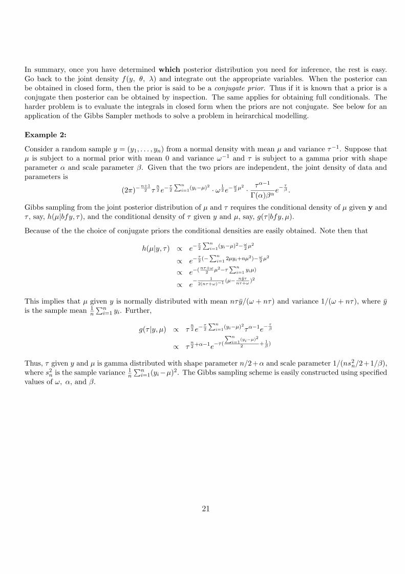
Example 2:

Consider a random sample y = (y1, . . . , yn) from a normal density with mean µ and variance τ−1. Suppose thatµ is subject to a normal prior with mean 0 and variance ω−1 and τ is subject to a gamma prior with shapeparameter α and scale parameter β. Given that the two priors are independent, the joint density of data andparameters is

(2π)−n+1

2 τn2 e−

τ2

∑n

i=1(yi−µ)2 · ω 1

2 e−ω2

µ2 · τα−1

Γ(α)βαe− τ

β .

Gibbs sampling from the joint posterior distribution of µ and τ requires the conditional density of µ given y andτ , say, h(µ|bfy, τ), and the conditional density of τ given y and µ, say, g(τ |bfy, µ).

Because of the the choice of conjugate priors the conditional densities are easily obtained. Note then that

h(µ|y, τ) ∝ e−τ2

∑n

i=1(yi−µ)2−ω

2µ2

∝ e−τ2(−∑n

i=12µyi+nµ2)−ω

2µ2

∝ e−( nτ+ω2

µ2−τ∑n

i=1yiµ)

∝ e− 1

2(nτ+ω)−1 (µ− nyτnτ+ω

)2

This implies that µ given y is normally distributed with mean nτy/(ω + nτ) and variance 1/(ω + nτ), where yis the sample mean 1

n

∑ni=1 yi. Further,

g(τ |y, µ) ∝ τn2 e−

τ2

∑n

i=1(yi−µ)2τα−1e

− τβ

∝ τn2+α−1e

−τ(

∑n

i=1(yi−µ)2

2+ 1

β)

Thus, τ given y and µ is gamma distributed with shape parameter n/2+α and scale parameter 1/(ns2n/2+1/β),

where s2n is the sample variance 1

n

∑ni=1(yi−µ)2. The Gibbs sampling scheme is easily constructed using specified

values of ω, α, and β.

21

References

Chib, S., and Greenberg, E. (1995),“Understanding the Metropolis-Hastings Algorithm,” The American Sta-tistician, 49, 327–335.

Gelfand, A. E., and Smith, A. F. M. (1990), “Sampling-Based Approaches to Calculating Marginal Densities,”Journal of the American Statistical Association, 85, 398–409.

Gelman, A. (1992), “Iterative and Non-Iterative Simulation Algorithms,” in Computing Science and Statistics(Interfact Proceedings), 24, 433–438.

Gelman, A., Carlin, D. B., Stern, H.S., and Rubin, D. B. (1995), Bayesian Data Analysis, Chapman &Hall:London

Gelman, A., and Rubin, D. B. (1992), “Inference from Iterative Simulation Using Multiple Sequences” (withdiscussion), Statistical Science, 7, 457–511.

Geman, S., and Geman, D. ((1984) “Stochastic Relaxation, Gibbs Distributions and the Bayesian Restorationof Images,” IEEE Transactions on Pattern Analysis and Machine Intelligence, 6, 721–741.

Geweke, J. (1989), “Bayesian inference in econometric models using Monte Carlo integration,” Econometrica,57, 1317-1340.

Gilks, W. R. , Richardson, S. and Spiegelhalter, D. J. [Ed.] (1996) Markov Chain Monte Carlo in Practice,Chapman & Hall:London.

Hastings, W. K. (1970), “Monte Carlo Sampling Methods Using Markov Chains and Their Applications,”Biometrika, 57, 97–109.

Metropolis, N., Rosenbluth, A. W., Rosenbluth, M. N., Teller, A. H., and Teller, E. (1953), “Equations of StateCalculations by Fast Computing Machines,” Journal of Chemical Physics, 21, 1087–1092.

Smith, A. F. M., and Roberts, G. O. (1993), “Bayesian Computation via the Gibbs Sampler and RelatedMarkov Chain Monte Carlo Methods,” Journal of the Royal Statistical Society, Scr. B, 55, 3–24.

Tanner, M. A., and Wong, W. H. (1987), “The Calculation of Posterior Distributions by Data Augmentation,”Journal of the American Statistical Association, 82, 528–549.

Tierney, L. (1994), “Markov Chains for Exploring Posterior Distributions” (with discussion), Annals of Statis-tics, 22, 1701–1762.

22