Statistically Valid Inferences from PrivacyProtected Data∗

Georgina Evans† Gary King‡

Margaret Schwenzfeier§ Abhradeep Thakurta¶

December 7, 2019

Abstract

Unprecedented quantities of data that could help social scientists understand andameliorate the challenges of human society are presently locked away inside compa-nies, governments, and other organizations, in part because of worries about privacyviolations. We address this problem with a general-purpose data access and analysissystem with mathematical guarantees of privacy for individuals who may be repre-sented in the data, statistical guarantees for researchers seeking population-level in-sights from it, and protection for society from some fallacious scientific conclusions.We build on the standard of “differential privacy” but, unlike most such approaches,we also correct for the serious statistical biases induced by privacy-preserving pro-cedures, provide a proper accounting for statistical uncertainty, and impose minimalconstraints on the choice of data analytic methods and types of quantities estimated.Our algorithm is easy to implement, simple to use, and computationally efficient; wealso offer open source software to illustrate all our methods.

∗The current version of this paper is available at GaryKing.org/dp. Many thanks for helpful com-ments to Adam Breuer, Merce Crosas, Cynthia Dwork, Max Golperud, Andy Guess, Kosuke Imai, DanKifer, Solomon Messing, Xiao-Li Meng, Nate Persily, Aaron Roth, Adam Smith, Salil Vadhan, SergeyYekhanin, and Xiang Zhou. Thanks also for help from the Alexander and Diviya Maguro Peer Pre-ReviewProgram at Harvard’s Institute for Quantitative Social Science.

†Ph.D. Candidate, Department of Government, Harvard University, 1737 Cambridge Street Cambridge,MA 02138; Georgina-Evans.com, GeorginaEvans@g.harvard.edu.

‡Albert J. Weatherhead III University Professor, Institute for Quantitative Social Science, 1737 Cam-bridge Street, Harvard University, Cambridge MA 02138; GaryKing.org, King@Harvard.edu.

§Ph.D. Candidate, Department of Government, Harvard University, 1737 Cambridge Street Cambridge,MA 02138; MegSchwenzfeier.com, schwenzfeier@g.harvard.edu.¶Assistant Professor, Department of Computer Science, University of California Santa Cruz,

bit.ly/AbhradeepThakurta, aguhatha@ucsc.edu.

1 Introduction

Just as more powerful telescopes empower astronomers, the accelerating influx of data

about the political, social, and economic worlds has enabled considerable social science

progress in understanding and ameliorating the challenges of human society. Yet, al-

though we have more data than ever before, we may now have a smaller fraction of the

data in the world than ever before because huge amounts are now locked up inside private

companies, in part because of privacy concerns (King and Persily, In press). If we are to

do our jobs as social scientists, we have no choice but to find ways of unlocking data from

industry, as well as from governments, nonprofits, and other researchers. We might hope

that government or society will take actions to support this mission, but we can also take

responsibility ourselves and begin to develop technological solutions to these political

problems.

In this paper, we develop methods to foster an emerging change in the paradigm for

sharing research information. Under the familiar data sharing regime, trusted researchers

simply obtain copies of data from others (perhaps with a data use agreement). Yet, with

the public’s increasing concerns over privacy, and data holders’ (companies, governments,

researchers, and others) desire to respond, this regime is failing. Fueling these concerns is

the discovery that the common practice of de-identification does not reliably protect indi-

vidual identities (Sweeney, 1997); nor does aggregation, query auditing, data clean rooms,

legal agreements, restricted viewing, paired programmer models, and others (Dwork and

Roth, 2014). And not only does the venerable practice of trusting researchers to follow

the rules fail spectacularly at times (like the Cambridge Analytica scandal, sparked by

a single researcher), but it turns out that even trusting a researcher who is known to be

trustworthy does not always guarantee privacy (Dwork and Ullman, 2018).

An alternative approach that may help persuade some data holders to allow academic

research is the data access regime. Under this regime, we begin with a trusted com-

puter server that holds confidential data and treats researchers as potential “adversaries,”

meaning that they may try to learn individuals’ private information while also seeking

knowledge for research to generate public good. Then we add a “differentially private”

1

algorithm that makes it possible for researchers to discover population-level insights but

impossible to reliably detect the effect of the inclusion or exclusion of any one individual

in the dataset or the value of any one person’s variables. Under this data access regime

researchers run statistical analyses on the server and receive “noisy” results computed by

this privacy-preserving algorithm, but are limited by the total number of runs they may

perform (so that they cannot repeat the same query many times and average away the

noise). Differential privacy is a widely accepted mathematical standard for data access

systems that promises to avoid some of the zero-sum policy debates over balancing the

interests of individuals with the public good that can come from research. It also seems

to satisfy regulators and others.1

A fast growing literature has formed around differential privacy, seeking to balance

privacy and utility, but the current measures of “utility” provide little utility to social sci-

entists or other statistical analysts. Statistical inference usually involves choosing a target

population of interest, identifying the data generation process, and then using the result-

ing dataset to learn about features of the population. Valid inferences require methods

with known statistical properties (such as unbiasedness, consistency, etc.) and honest as-

sessments of uncertainty (e.g. standard errors). In contrast, privacy researchers typically

begin with the choice of a target (confidential) dataset, add privacy-protective procedures,

and then use the resulting differentially private dataset or analyses to infer to the confi-

dential dataset — usually without regard to the data generation process or valid population

inferences. This approach is useful for designing privacy algorithms but, as Wasserman

(2012) puts it, “I don’t know of a single statistician in the world who would analyze data

this way.”2

1Differential privacy was introduced by Dwork, McSherry, et al. (2006) and generalizes the social sci-ence technique of “randomized response” to elicit sensitive information in surveys (see Blair, Imai, andZhou, 2015; Glynn, 2013; Warner, 1965); see Dwork and Roth (2014) and Vadhan (2017) for overviewsand Wood et al. (2018) for a nontechnical introduction.

2“In statistical inference the sole source of randomness lies in the underlying model of data generation,whereas the estimators themselves are a deterministic function of the dataset. In contrast, differentiallyprivate estimators are inherently random in their computation. Statistical inference that considers both therandomness in the data and the randomness in the computation is highly uncommon” (Sheffet, 2017). AsKarwa and Vadhan (2017) write, “Ignoring the noise introduced for privacy can result in wildly incorrectresults at finite sample sizes. . . this can have severe consequences.” On the essential role of inference anduncertainty and in science, see King, Keohane, and Verba (1994).

2

To make matters worse for social scientists, most privacy-protective procedures induce

severe bias in population inferences, and even in inferences to features of confidential

datasets. These include adding random error, which induces measurement error bias,

and censoring (known as “clamping” in computer science), which induces selection bias

(Blackwell, Honaker, and King, 2017; Stefanski, 2000; Winship and Mare, 1992). We

have not found a single prior study that tries to correct for both (although some avoid the

effects of censoring in theory at the cost of additional noise in practice; Karwa and Vadhan

2017; Smith 2011) and few have accurate uncertainty estimates. This is crucial because

inferentially invalid data access systems can harm societies, organizations, and individuals

— such as by inadvertently encouraging the distribution of misleading medical, policy,

scientific, and other conclusions — even if it successfully protects individual privacy. For

these reasons, using systems presently designed to ensure differential privacy would be

unattractive for social science analysis.3

Social scientists and others need algorithms on data access systems with both infer-

ential validity and differential privacy. We offer one such algorithm that is approximately

unbiased, has lower variance than uncorrected estimates, and comes with accurate uncer-

tainty estimates. The algorithm also turns censoring from a feature that severely biases

statistical estimates in order to protect privacy to an attractive feature that greatly reduces

the amount of noise needed to protect privacy while still leaving estimates approximately

unbiased. The algorithm is easy to implement, computationally efficient even for very

large datasets, and, because the entire dataset never needs to be stored in the same place,

may offer additional security protections.

Our algorithm is generic, designed to minimally restrict the choice among statistical

procedures, quantities of interest, data generating processes, and statistical modeling as-

sumptions. Because the algorithm does not constrain researcher choices in these ways,

3Inferential issues also affect differential privacy applications outside of data access systems (the socalled “global model”). These include “local model” systems where private calculations are made on auser’s system and sent back to a company in a way that prevents it from making reliable inferences aboutindividuals — including Google’s Chrome (Erlingsson, Pihur, and Korolova, 2014) and their other coreproducts (Wilson et al., 2019), Apple’s MacOS (Tang et al., 2017), and Microsoft’s Windows (Ding, Kulka-rni, and Yekhanin, 2017) — and the US Census Bureau’s efforts to release differentially private datasets(Garfinkel, Abowd, and Powazek, 2018).

3

it may be especially well suited for building data access systems designed for research.

When valid inferential methods exist or are developed for more restricted use cases, they

may sometimes allow less noise for the same privacy guarantee. As such, one produc-

tive plan for building a general-purpose data access system may be to first implement our

algorithm and to then gradually add these more specific approaches when they become

available as preferred choices.4

We offer an introduction to differential privacy and describe the inferential challenges

in analyzing data from a differentially private data access system, in Section 2. We give

a generic differentially private algorithm in Section 3 which, like most such algorithms,

is statistically biased. We therefore introduce bias corrections and variance estimators in

Section 4 together with the private algorithm accomplishes our goals. We illustrate the

performance of this approach in finite samples via Monte Carlo simulations in Section 5

and offer practical advice for implementation and use in Section 6. Appendices add tech-

nical details. We are also making available open source software (called UnbiasedPrivacy)

to illustrate all the methods described herein.

2 Differential Privacy and its Inferential Challenges

We now define the differential privacy standard, describe its strengths, and highlight the

challenges it poses for proper statistical inference. Throughout, we modify notation stan-

dard in computer science so that it is more familiar to social scientists.

2.1 Definitions

Begin with a confidential dataset D, defined as a collection of N rows of numerical mea-

surements constructed so that each individual whose privacy is to be protected is repre-

4For example, Karwa and Vadhan (2017) develop finite sample confidence intervals with proper cover-age for the mean of a normal density; Barrientos et al. (2019) offer differentially private significance testsfor linear regression coefficients; Gaboardi et al. (2016) propose chi-squared tests for goodness of fit testsfor multinomial data and independence between two categorical variables; Smith (2011) shows that, for aspecific class of estimators and of data generating processes, there exists a differentially private estimatorwith the same asymptotic distribution; Wang, Lee, and Kifer (2015) propose accurate p-values for chi-squared tests of independence between two variables in tabular data; Wang, Kifer, and Lee (2018) developdifferentially private confidence intervals for objective or output perturbation; and Williams and McSherry(2010) provide an elegant marginal likelihood approach for moderate sized datasets.

4

sented in at most one row.5

Statistical analysts would normally calculate a statistic s (such as a count, mean, pa-

rameter estimate, etc.) from D as a fixed number, say s(D). For inference, they then

conceptualize s(D) as a random variable given (hypothetical, unobserved) repeated draws

of D following the same data generation process from a population. In contrast, privacy

analysts ignore populations and data generation processes and treat s(D) as the fixed un-

observed quantity of interest. They then construct a “mechanism” M(s,D), which is a

privacy-protected version of the same statistic, calculated by injecting carefully calibrated

noise and censoring at some point before returning the result. As we will show, the specific

types of noise and censoring are specially designed to satisfy differential privacy. Privacy

researchers conceptualize (hypothetical, unobserved) sampling distributions of M(s,D),

but these are generated by repeated draws of the noise from the same distribution, with D

fixed.

Meeting the differential privacy standard prevents a researcher from reliably learning

anything different from a dataset regardless of whether an individual has been included or

excluded. To formalize this notion, consider two datasets D and D′ that differ in at most

one row (a maximum Hamming distance of 1). Then, the standard requires that the proba-

bility (or probability density) of any analysis result m from dataset D, Pr[M(s,D) = m],

be indistinguishable from the probability that the same result is produced by the same

analysis of dataset D′, Pr[M(s,D′) = m], where the probabilities take D as fixed and are

computed over the noise.

We write an intuitive version of the differential privacy standard (using the fact that

eε ≈ 1 + ε for small ε) by defining “indistinguishable” as the ratio of the probabilities

falling within ε of equality (which is 1). Thus, a mechanism is said to be ε-differentially

private ifPr[M(s,D) = m]

Pr[M(s,D′) = m]∈ 1± ε, (1)

where ε is a pre-chosen level of possible privacy leakage, with smaller values potentially

5Hierarchical data structures, or dependence among units, is allowed within but not between rows. Forexample, rows could represent a family with variables for different family members.

5

giving away less privacy (by requiring more noise or censoring).6 Many variations and

extensions of Equation 1 have been proposed (Desfontaines and Pejó, 2019). We use the

most popular, known as “(ε, δ)-differential privacy” or “approximate differential privacy,”

which adds a very small chosen offset δ to the numerator of the ratio in Equation 1. This

second privacy parameter, which the user chooses such that δ < 1/N , turns out to al-

low mechanisms with (statistically convenient) Gaussian noise processes. This relaxation

also has Bayesian interpretations, with the posterior distribution of M(s,D) close to that

of M(s,D′), and also that an (ε, δ)-differentially private mechanism is ε-differentially

private with probability at least 1 − δ (Vadhan, 2017, p.355ff). We can also express ap-

proximate differential privacy more formally as requiring that each of the probabilities be

bounded by a linear function of the other:7

Pr[M(s,D) = m] ≤ δ + eε · Pr[M(s,D′) = m]. (2)

Consistent with political science research showing that secrecy is best thought of on a

continuum (Roberts, 2018), the differential privacy standard quantifies the privacy leakage

of a given mechanism via the choices of ε and δ. Differential privacy is expressed in terms

of the maximum possible privacy loss, but the expected privacy loss is considerably less

than this worst case analysis, often by orders of magnitude (Carlini et al., 2019; Jayaraman

and Evans, 2019). It also protects small groups in the same way as individuals, with

the maximum risk kε dropping linearly in group size k. And because mechanisms with

different small values of ε have similar properties, even some violations of the differential

privacy standard may still be differentially private for larger values of ε and δ.

6Using this multiplicative (ratio) metric to indicate what is “indistinguishable” turns out to be muchmore protective of individual privacy than some others, such as an additive (difference) metric. For example,consider an obviously unacceptable mechanism: “choose one individual uniformly at random and discloseall of his or her data.” This mechanism is not differentially private (the ratio can be infinite and thus greaterthan any finite ε), but it may seem safe on an additive metric because the impact of adding or removing oneindividual on the difference in the probability distribution of a statistical output is proportional to at most1/N .

7Our algorithms below also satisfy a strong version of approximate differential privacy known as Rényidifferential privacy; see Mironov (2017).

6

2.2 Example

The literature includes many differentially private mechanisms. These add noise and cen-

soring to the data inputs, the output estimates, or various parts of internal calculations,

such as the gradients, elements of X ′X matrices for regression, or others. For the goal

of developing a generic algorithm, we now introduce the differentially private Gaussian

mechanism, which we use throughout this paper. This mechanism, like most others, is

statistically biased and inconsistent and does not come with uncertainty estimates, but we

will use a version of it in Section 3 to build a differentially private algorithm and then

provide corrections in Section 4 to make it statistically valid.

To fix ideas, consider a confidential database of the incomes of people in a neighbor-

hood of Seattle and the mean income as the target quantity of interest: y = 1N

∑Ni=1 yi.

Given the researcher’s choice of privacy parameters ε and δ and bounding parameter

Λ > 0, we define this as the censored mean plus Gaussian noise:

M(mean, D) = θ +N (0, S2) (3)

with mean θ = 1N

∑Ni=1 c(yi,Λ) and censoring function

c(y,Λ) =

{y if y ∈ [−Λ,Λ]

sgn(y)Λ if y /∈ [−Λ,Λ].(4)

The remaining question is how much noise to add or, in other words, the definition of

S ≡ S(Λ, ε, δ, N). Under approximate differential privacy, we add only as much noise

as necessary to satisfy Equation 2, which we write for this purpose as N (t | θ, S2) ≤

δ + eε · N (t | θ + ∆, S2), where ∆ is the sensitivity of this estimator (the largest change

over all possible pairs of datasets that differ by at most one row), where |θD − θD′| ≤ ∆

such that θD and θD′ denote the estimator computed from D and D′, respectively. The

censored mean θ has sensitivity ∆ = 2Λ/N .

Although in practice, we recommend a more general solution with a tight bound,8 the8Dwork and Roth (2014) show that Equation 5 holds only for ε ≤ 1. For any value of ε, we recommend

the tight bound based on the numerical solution by Balle and Wang (2018) which allows much smallervalues of S even when ε ≤ 1. As a brief summary, note that if M is Gaussian, then Equation 2 can bewritten in terms of the cumulative standard normal density: Φ

(∆2σ −

εσ∆

)− eεΦ

(− ∆

2σ −εσ∆

)≤ δ. Then set

S equal to the minimum σ satisfying this inequality. A clear benefit is that the solution exactly calibrates thenoise to a given privacy budget and hence minimizes the variance of the output for a given level of {ε, δ}.The cost of this approach is computing a unique numerical solution for each run of their algorithm.

7

simplest solution gives

S ≡ S(Λ, ε, δ, N) =∆√

2 ln(1.25/δ)

ε=

2Λ√

2 ln(1.25/δ)

Nε. (5)

For intuition, we also simplify further with an arbitrary but convenient choice for δ:

S(Λ, ε, 0.0005, N) ≈ 8Λ

Nε. (6)

Equation 6 shows that, to protect the biggest possible outlier, differential privacy allows

us to add less noise if each person is submerged in a sea of many others (larger N ), if less

privacy is required (larger ε), or if more censoring is used (smaller Λ).

With any level of censoring, θ is obviously a biased estimate of y: E(θ) 6= y. To

reduce censoring and thus bias, we can choose larger values of Λ but that unfortunately

would increase the noise, the statistical variance, and our uncertainty estimates; similarly,

reducing noise by choosing a smaller value of Λ increases the impact of censoring. These

choices are important: if the largest outlier could be Bill Gates or Jeff Bezos, then avoiding

censoring would require adding so much noise that it would swamp any relevant signal

from the data. We resolve much of this tension Section 4.

2.3 Inferential Challenges

We now discuss four issues the tools of differential privacy pose from the perspective of

statistical inference. For some we offer corrections; for others, we suggest how to adjust

statistical analysis practices.

First, censoring data induces selection bias in statistical inference. Avoiding censoring

by adding more noise is no solution because any amount of noise induces bias in statis-

tical estimators for nonlinear functions of the data. Moreover, even for estimators that

are unbiased (like the mean in Section 2.2), the added noise makes unadjusted standard

errors statistically inconsistent. Ignoring either measurement error bias or selection bias

is usually a major inferential mistake and may change substantive conclusions, the prop-

erties of estimators, and the validity of uncertainty estimates, often in negative, unknown,

or surprising ways.9

9For example, adding mean-zero noise to one variable or its mean induces no bias in estimating the

8

Second, uncertainty estimators are rarely proposed or even discussed in the literature

on differentially private mechanisms. Unfortunately, accurate uncertainty estimates can-

not be generated by using differentially private versions of classical uncertainty estimates.

To be more specific, in a system without differential privacy, let θ be a point estimate in

an observed dataset of a quantity of interest θ from an unobserved population. Denote

by V (θ) the variance of θ over repeated (hypothetical, unobserved) samples of datasets

drawn with the same data generation process from the population, with an estimate from

the one observed dataset V (θ), its square root being the standard error, a commonly re-

ported measure of statistical uncertainty. For a proper scientific statement, it would be

sufficient to have (1) an estimator θ with known statistical properties (such as unbiased-

ness, consistency, efficiency, etc.), and (2) a variance estimate V (θ) that reflects the true

variance V (θ). Consider now the differentially private point estimate θdp. Although it

would be easy to compute a differentially private variance estimate V (θ)dp using the same

type of mechanism, it is of no direct use, since θ is never disclosed and so its variance is

irrelevant. Indeed, V (θ)dp is a biased estimate of the relevant uncertainty, V (θdp). Since

we will show below that θdp itself is biased, V (θdp) would be of no direct use even if it

were known.

Third, to avoid researchers rerunning the same analysis many times and averaging

away the noise, their analyses must be limited. This limitation is formalized via a differ-

ential privacy property known as composition: If mechanism k is (εk, δk)-differentially pri-

vate, for k = 1, . . . , K, then disclosing allK estimates is (∑K

k=1 εk,∑K

k=1 δk)-differentially

private.10 Then the restriction is implemented via a quantitative privacy budget in which

the data provider allocates a total value of ε to a researcher who can then divide it up and

run as many analyses, of whatever type, as they choose, so long as the sum of all the εs

population mean, but adding noise to its variance creates a biased estimate. The estimated slope coefficientin a simple regression of y on x where, with random measurement error in x, is biased toward zero; if weadd variables with or without measurement error to this regression, the same coefficient can be biased byany amount and in any direction. Censoring sometimes attenuates causal effects but it can also exaggeratethem; predictions and estimates of other quantities of interest can be too high, too low, or have their signschanged. Measurement error and censoring should not be ignored; they do not come out in the wash.

10Alternatively, if the K quantities are disclosed simultaneously and returned in a batch, then we couldchoose to set the variance of the error for all together at a higher individual level but lower collective level,dependent also on the type of noise added (Bun and Steinke, 2016; Mironov, 2017).

9

across all their analyses does not exceed their total privacy budget.

This strategy has the great advantage of enabling each researcher to make these choices,

rather than a central authority such as the data provider. However, when the total privacy

budget is used up, no researcher can ever run a new analysis on the same data unless the

data provider chooses to increase the budget. This constraint is a useful feature to protect

privacy, but it utterly changes the nature of statistical analysis. To see this, note that best

practice recommendations have long included trying to avoid being fooled by the data —

by running every possible diagnostic, fully exploring the dataset, and conducting numer-

ous statistical checks — and by the researcher’s personal biases — such as by preregistra-

tion ex ante to constrain the number of analyses that will be run to eliminate “p-hacking”

or correcting for “multiple comparisons” ex post (Monogan, 2015). One obviously needs

to avoid being fooled in any way, and so researchers normally try to balance the result-

ing contradictory advice to avoid each problem. In contrast, differential privacy tips the

scales: Remarkably, it makes solving the second problem almost automatic (Dwork, Feld-

man, et al., 2015), but it also severely reduces the probability of serendipitous discovery

and increases the odds of being fooled by unanticipated data problems. Successful data

analysis with differential privacy thus requires careful planning, although less stringently

than with pre-registration.

Finally, a researcher can learn about an individual from a differentially private mech-

anism, but no more than if that individual were excluded from the data set. For example,

suppose research indicates that women are more likely to share fake news with friends on

social media than men; then, if you are a woman, everyone knows that you have a higher

risk of sharing fake news. But the researcher would have learned this population-level fact

whether or not you were included in the dataset and so you have no reason to withhold

your information.

However, we must also be certain that the differentially private mechanism is infer-

entially valid. If researchers use privacy preserving mechanisms that bias statistical pro-

cedures and no corrections are applied, society can sometimes be mislead and numerous

individuals can be hurt by publishing incorrect population level inferences. (In fact, it is

10

older people, not women, who are more likely to share fake news! See Guess, Nagler,

and Tucker 2019.) Fortunately, all of differential privacy’s properties are preserved under

post-processing, which means that no privacy loss will occur when, below, we correct

for inferential biases induced by noise and censoring (or if results are published or mixed

with any other data sources). In particular, for any data analytic function f not involv-

ing private data D, if M(s,D) is differentially private, then f [M(s,D)] is differentially

private, regardless of assumptions about potential adversaries or threat models.

Although differential privacy may seem to follow a “do no more harm” principle,

careless use of this technology can in fact harm individuals and society if we do not also

ensure inferential validity. The biases from ignoring measurement error and selection

can each separately or together reverse, attenuate, exaggerate, or nullify statistical results.

Helpful medical treatments could be discarded. Harmful practices may be promoted. Of

course, when providing access to confidential data, not using differential privacy may

also have grave costs to individuals. Data providers must therefore ensure that data access

systems are both differentially private and inferentially valid.

3 A Generic Differentially Private Estimator

Our approach, which like our software we call UnbiasedPrivacy (or UP), has two parts —

a differentially private mechanism introduced in this section and a bias correction of the

differentially private result, using the algorithm in Section 4. Section 4 also gives accurate

uncertainty estimates in the form of standard errors.

Let D denote a population data matrix, from which N observations are selected to

form our observed data matrix D. Our goal is to estimate some (fixed scalar) quantity

of interest, θ = s(D) with the researcher’s choice of statistical procedure s (among the

vast array that are statistically valid under bootstrapping, i.e., any statistic with a positive

bounded second Gateaux derivative and Hadamard differentiability; see Wasserman 2006,

p.35). Let θ = s(D) denote an estimate of θ computed from the private data in the way we

normally would without privacy protective procedures. Because privacy concerns prevent

θ from being disclosed, we show here instead how to estimate a differentially private

11

estimate of θ denoted θdp which, like many such estimators, is substantially biased but is

bias corrected in the next section.

To estimate, θdp, the user chooses a statistical method (logit, regression, cross-tabulation,

etc.), a quantity of interest estimated from the statistical method (causal effect, risk differ-

ence, predicted value, etc.), and values for each of the privacy parameters, Λ, ε, and δ (see

Section 6 for advice on making these choices).

We give the details of our proposed mechanism M(s,D) = θdp in Section 3.1. It uses

a partitioning version of the “sample and aggregate” algorithm (Nissim, Raskhodnikova,

and Smith, 2007), to ensure differential privacy for almost any statistical method and

quantity of interest. We also incorporate an optional application of the computationally

efficient “bag of little bootstraps” algorithm (Kleiner et al., 2014), that will ensure an

aspect of inferential validity generically, by not having to worry about differences in how

to scale up different statistics from each partition to the entire dataset.

3.1 Mechanism

Randomly partition rows ofD as {D1, . . . , DP}, each of subset size n ≈ N/P (we discuss

the choice of P below), and then follow this algorithm.

1. For partition p (p = 1, . . . , P )

(a) Compute an estimate θp (of a quantity of interest θ) either directly (being

careful to appropriately scale up quantities that require it; see Section 3.3) or

by bootstrapping (where scaling up is automatic) as follows:

i. For bootstrap simulation b (b = 1, . . . , B)

A. Simulate bootstrap b by sampling one weight for each of the n units

in partition p as: wb ≡ {w1,b, . . . , wn,b} ∼ Multinomial(N,1n/n).

B. Calculate a statistic (an estimate of population value θ) from boot-

strapped sample b in partition p: θp,b = s(Dp, wb), such as a predicted

value, expected value, or classification.

ii. Summarize the set of bootstrapped estimates within each partition with

an (unobserved, nonprivate) estimator, which we write generically as θp.

12

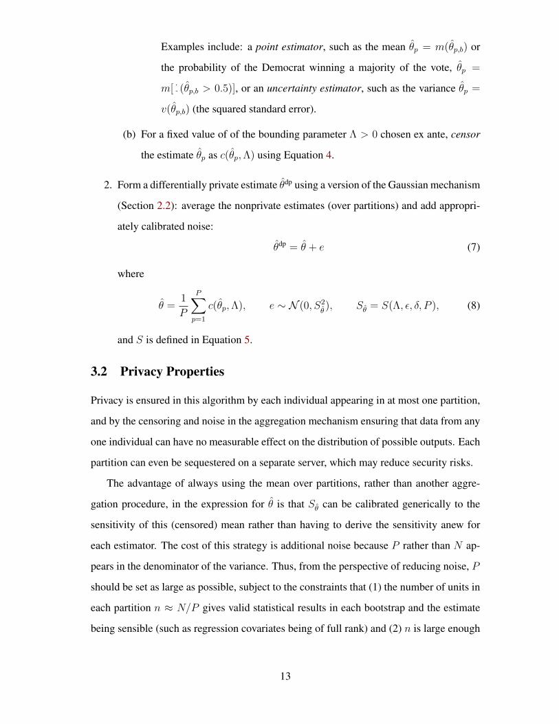
Examples include: a point estimator, such as the mean θp = m(θp,b) or

the probability of the Democrat winning a majority of the vote, θp =

m[1(θp,b > 0.5)], or an uncertainty estimator, such as the variance θp =

v(θp,b) (the squared standard error).

(b) For a fixed value of of the bounding parameter Λ > 0 chosen ex ante, censor

the estimate θp as c(θp,Λ) using Equation 4.

2. Form a differentially private estimate θdp using a version of the Gaussian mechanism

(Section 2.2): average the nonprivate estimates (over partitions) and add appropri-

ately calibrated noise:

θdp = θ + e (7)

where

θ =1

P

P∑p=1

c(θp,Λ), e ∼ N (0, S2θ), Sθ = S(Λ, ε, δ, P ), (8)

and S is defined in Equation 5.

3.2 Privacy Properties

Privacy is ensured in this algorithm by each individual appearing in at most one partition,

and by the censoring and noise in the aggregation mechanism ensuring that data from any

one individual can have no measurable effect on the distribution of possible outputs. Each

partition can even be sequestered on a separate server, which may reduce security risks.

The advantage of always using the mean over partitions, rather than another aggre-

gation procedure, in the expression for θ is that Sθ can be calibrated generically to the

sensitivity of this (censored) mean rather than having to derive the sensitivity anew for

each estimator. The cost of this strategy is additional noise because P rather than N ap-

pears in the denominator of the variance. Thus, from the perspective of reducing noise, P

should be set as large as possible, subject to the constraints that (1) the number of units in

each partition n ≈ N/P gives valid statistical results in each bootstrap and the estimate

being sensible (such as regression covariates being of full rank) and (2) n is large enough

13

and growing faster than P (to ensure the central limit theorem can be applied). (Subsam-

pling itself increases the variance of nonlinear estimators, but usually much less than the

increased variance due to privacy protective procedures; see also Mohan et al. (2012) for

more formal methods of optimizing P .)

3.3 Inferential Properties

The statistical properties of estimators from our algorithm differ depending on type. For

example, consider two conditions: (1) an assumption we maintain until the next section

that Λ is large enough so that censoring has no effect (c(θp,Λ) = θp), and (2) an estimator

applied to the private data that is unbiased for the chosen quantity of interest. If these

two conditions hold, and because also we are injecting additive noise at the last stage of

the mechanism (rather in the data, the objective function, sequential steps, etc.), the point

estimates are unbiased:

E(θdp) =1

P

P∑p=1

E(θp) + E(e) = θ. (9)

In practice, however, choosing the bounding parameter Λ involves a bias-variance

trade-off: If Λ is set to the maximum possible sensitivity, censoring has no effect and θdp

is unbiased, but the noise is large (see Equation 8). Choosing smaller values of Λ reduce

noise, which reduces the variance of the estimator, but it simultaneously increases bias

due to censoring (Section 3, Step 1b). Also, if the estimator is applied without privacy

protective procedures is biased (such as by violating statistical assumptions or merely

being a nonlinear function of the data), then our algorithm will not magically remove the

bias, but it will not add bias.

In contrast, uncertainty estimators require adjustment even if the three conditions

are met. For example, the variance of the differentially private estimator is V (θdp) =

V (θ) + S2θ, but its naive variance estimator (the differentially private version of an unbi-

ased nonprivate variance estimator) is biased:

E[V (θ)dp

]= E

[V (θ) + e

]= V (θ) + E(e) = V (θ) 6= V (θdp). (10)

Fortunately, we can compute an unbiased estimate of the variance of the differentially

private estimator by simply adding back in the (known) variance of the noise: V (θdp) =

14

V (θ)+S2θ, which is unbiased: E

[V (θdp)

]= V (θdp). Of course, because (2) will typically

be violated, and the resulting censoring will bias our estimates, we must bias correct this

estimate and then compute the variance of the corrected estimate, which will ordinarily

require a more complicated expression.

Finally, as indicated in the algorithm, the “little bag of bootstraps” in algorithm step

1(a) can be replaced with the choice of an unbiased estimator applied directly to data

within partition p, if estimators are scaled up appropriately by modifying Equation 7 to

match the size of the entire dataset (see Politis, Romano, and Wolf, 1999). On the one

hand, the bootstrap approach is simpler in two situations. First, the necessary scale factors

the researcher would need to derive without bootstrapping differ depending on the type of

estimator and quantity of interest; some quantities, like the variance, are a linear function

of N , but each partition’s estimate is a function of n and so need to be scaled up by a fac-

tor of (N − n)/n. In contrast, the bootstrapping approach can be applied generically, the

same for all. Second, bootstrapping allows simpler and more flexible estimation strate-

gies for some quantities, such as the probability that a causal effect is greater than zero,

estimated by merely counting the proportion of positive bootstrap estimates that meet se-

lected criteria. (It works well for estimating α2 in the model below when P is unavoidably

small and so would otherwise create grouping error.) On the other hand, some quantities

that without differential privacy would be easy to compute with bootstrapping are difficult

or impossible with differential privacy, such as the variance of post-processed quantities,

like our bias corrected estimator.11

4 Valid Statistical Inference from Private Data

We develop here an approach to valid inference from private data using a post-processed

version of the generic differentially private estimator developed in Section 3, which means

it retains all of its privacy preserving properties. The post-processing bias corrects θdp for

11We also note that setting B = 1 (for a single bootstrap) would save computation but would make somequantities (such as the standard error or a predicted probability of a plurality vote for a candidate) impossibleto estimate by bootstrapping and would be inefficient even for those that are possible; alternatively, replacingthe weights in Step 1(a)i,A with a large dataset of size N constructed from each partition would satisfy thescaling issue but would require P times as much memory for each of the P computations.

15

censoring, and results in our estimator, θdp. We know of no prior attempt to correct for

biases due to censoring in differentially private mechanisms. This bias correction has the

effect of reducing the impact of whatever value of Λ is selected, and allows users to choose

smaller values to reduce variance and use less of the privacy budget without bias concerns

(see also Section 6). It even turns out that the variance of this bias corrected estimate is

actually smaller than the uncorrected estimate, which is unusual for bias corrections. We

also offer an estimate of this variance, denoted V (θdp).

4.1 Bias Correction

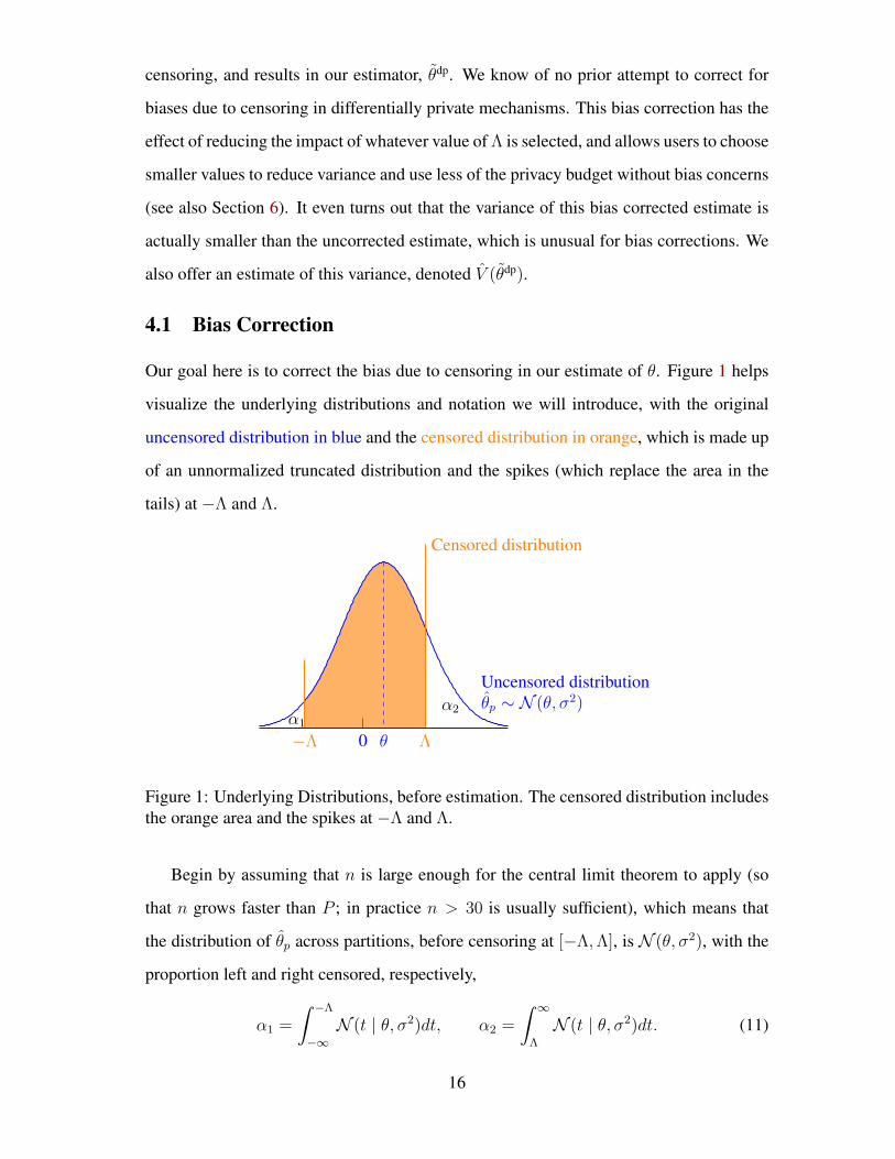
Our goal here is to correct the bias due to censoring in our estimate of θ. Figure 1 helps

visualize the underlying distributions and notation we will introduce, with the original

uncensored distribution in blue and the censored distribution in orange, which is made up

of an unnormalized truncated distribution and the spikes (which replace the area in the

tails) at −Λ and Λ.

Λ−Λ θ0

Censored distribution

Uncensored distributionθp ∼ N (θ, σ2)α2

α1

Figure 1: Underlying Distributions, before estimation. The censored distribution includesthe orange area and the spikes at −Λ and Λ.

Begin by assuming that n is large enough for the central limit theorem to apply (so

that n grows faster than P ; in practice n > 30 is usually sufficient), which means that

the distribution of θp across partitions, before censoring at [−Λ,Λ], is N (θ, σ2), with the

proportion left and right censored, respectively,

α1 =

∫ −Λ

−∞N (t | θ, σ2)dt, α2 =

∫ ∞Λ

N (t | θ, σ2)dt. (11)

16

We then write the expected value of θdp as the weighted average of the mean of the trun-

cated normal and of the spikes at −Λ and Λ:

E(θdp)

= −α1Λ + (1− α2 − α1)θT + α2Λ, (12)

with truncated normal mean

θT = θ +

σ√2π

[exp

(−1

2

(−Λ−θσ

)2)− exp

(−1

2

(Λ−θσ

)2)]

1− α2 − α1

. (13)

After substituting our point estimate θdp for the expected value in Equation 12, we are

left with three equations (12 and the two in 11) and four unknowns (θ, σ, α1, and α2).

We therefore use some of the privacy budget to obtain an estimate of α2 (or to increase

numerical stability we can try to estimate the larger of α1 or α2). Then we have three

equations and three unknowns (θ, σ, α1), which our open source software solves with a

fast numerical solution, giving θdp, which is our goal, the approximately unbiased estimate

of θ, along with estimates σdp and αdp1 .

For estimation, we note that α2 is bounded to the unit interval, and so we could set

Λα = 1 without risk of censoring, but this would overstate this parameter’s sensitivity by

a factor of two. Instead of resolving this issue by changing the expression for censoring

and S, we do so more conveniently, without changing the notation (or code) above, by

simply reparameterizing as β = α2 − 0.5, setting Λβ = 0.5, estimating and disclosing β,

and then solving to obtain our estimate of α2 before using it to solve our three equations.

4.2 Variance Estimation

We now derive a procedure for computing an estimate of the variance of our estimator,

V (θdp), without any additional privacy budget expenditure. We have the two directly es-

timated quantities, θdp and αdp2 , and the three (deterministically post-processed) functions

of these computed during bias correction: θdp, σ2dp, and αdp

1 . We then use standard simu-

lation methods (King, Tomz, and Wittenberg, 2000): We treat the estimated quantities as

random variables, bias correct to generate the others, and take the sample variance of the

simulations of θdp.

17

Thus, to represent estimation uncertainty, we draw the random quantities from a mul-

tivariate normal with plug-in parameter estimates. Using notation (i) to denote the ith

simulation, we write:

θdp(i), αdp2 (i) ∼ N

([θdp

αdp2

],

[V (θdp) Cov(αdp

2 , θdp)

Cov(αdp2 , θ

dp) V (αdp2 )

]). (14)

To implement this procedure we require V (θdp), V (αdp2 ), and Cov(αdp

2 , θdp), which we

show in Appendix A can be written as functions of information already disclosed. We plug

these into Equation 14 and repeatedly draw {θdp(i), αdp2 (i)}, each time bias correcting via

the procedure in Section 4.1 to compute θdp(i). Finally, we compute the sample variance

over these simulations to yield our estimate V (θdp).

5 Simulations

In this section, we evaluate the finite sample properties of our estimator via simple Monte

Carlo simulations. We show that while (uncorrected) differentially private point estimates

are inferentially invalid, our (bias corrected) estimators are approximately unbiased (when

the non-private estimator is unbiased), and come with accurate uncertainty estimates. In

addition, in part because our bias correction uses an additional disclosed parameter esti-

mate (α2), the variance of our estimator is usually lower than the variance of the uncor-

rected estimator.

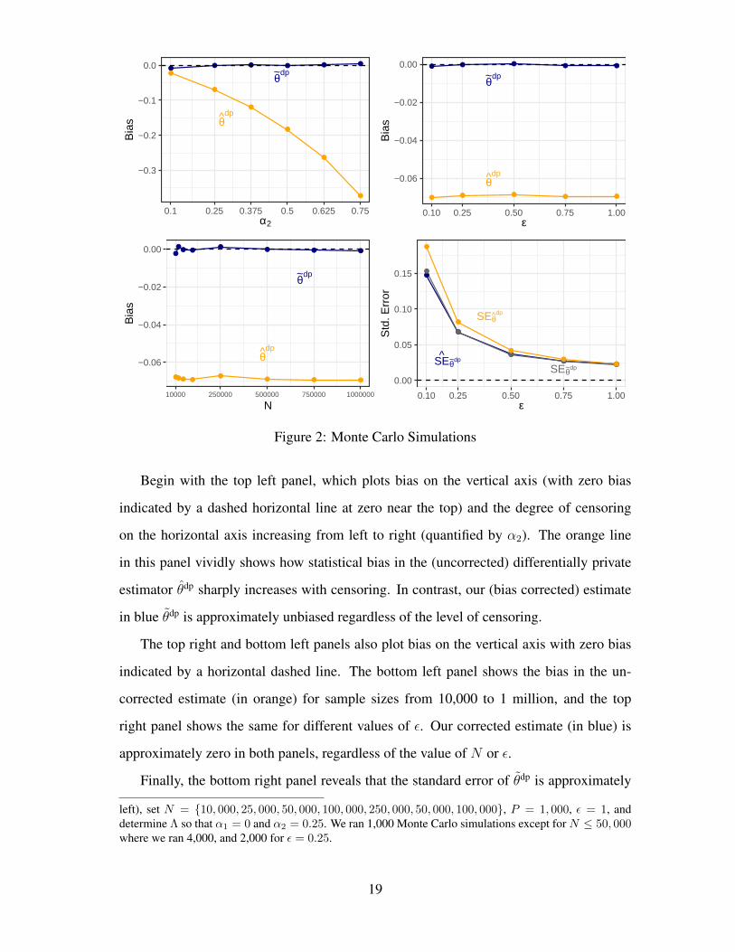
The results appear in Figure 2, which we discuss after first detailing the data generation

process. For four different types of simulations (in separate panels of the figure), we draw

data for each row i from an independent linear regression model: yi ∼ N (1 + 3xi, 102),

with xi ∼ N (0, 72) drawn once and fixed across simulations. Our chosen quantity of

interest is the coefficient on xi with value θ = 3. We study the bias of the (uncorrected)

differentially private estimator θdp, and our corrected version, θdp, as well as their standard

errors.12

12We have tried different parameter values, functional forms, and distributions, all of which led tothe same substantive conclusions. In Figure 2, for censoring (top left panel), we let α1 = 0, α2 ={0.1, 0.25, 0.375, 0.5, 0.625, 0.75}, N = 100, 000, P = 1, 000, and ε = 1. For privacy (in the topright panel) and standard errors (bottom right), let ε = {0.1, 0.15, 0.20, 0.30, 0.50, 1}, while settingN = 100, 000, P = 1, 000, and with Λ set so that α1 = 0 and α2 = 0.25. For sample size (bottom

18

●● ● ● ● ●

●

●

●

●

●

●

θdp

θ~dp

−0.3

−0.2

−0.1

0.0

0.1 0.25 0.375 0.5 0.625 0.75α2

Bia

s

● ● ● ● ●

● ● ● ● ●

θ~dp

θdp

−0.06

−0.04

−0.02

0.00

0.10 0.25 0.50 0.75 1.00ε

Bia

s

●

●● ●

● ● ● ●

●●● ●●

● ● ●

θdp

θ~dp

−0.06

−0.04

−0.02

0.00

10000 250000 500000 750000 1000000

N

Bia

s

●

●

●

●●

●

●

●●

●

●

●

●

●●

SEθdp

SEθ~dp

SEθ~dp

0.00

0.05

0.10

0.15

0.10 0.25 0.50 0.75 1.00ε

Std

. Err

or

Figure 2: Monte Carlo Simulations

Begin with the top left panel, which plots bias on the vertical axis (with zero bias

indicated by a dashed horizontal line at zero near the top) and the degree of censoring

on the horizontal axis increasing from left to right (quantified by α2). The orange line

in this panel vividly shows how statistical bias in the (uncorrected) differentially private

estimator θdp sharply increases with censoring. In contrast, our (bias corrected) estimate

in blue θdp is approximately unbiased regardless of the level of censoring.

The top right and bottom left panels also plot bias on the vertical axis with zero bias

indicated by a horizontal dashed line. The bottom left panel shows the bias in the un-

corrected estimate (in orange) for sample sizes from 10,000 to 1 million, and the top

right panel shows the same for different values of ε. Our corrected estimate (in blue) is

approximately zero in both panels, regardless of the value of N or ε.

Finally, the bottom right panel reveals that the standard error of θdp is approximately

left), set N = {10, 000, 25, 000, 50, 000, 100, 000, 250, 000, 50, 000, 100, 000}, P = 1, 000, ε = 1, anddetermine Λ so that α1 = 0 and α2 = 0.25. We ran 1,000 Monte Carlo simulations except for N ≤ 50, 000where we ran 4,000, and 2,000 for ε = 0.25.

19

correct (i.e., equal to the true standard deviation across estimates, which can be seen

because the blue and gray lines are almost on top of one another). It is even smaller for

most of the range than the standard error of the uncorrected estimate θdp.

These simulations suggest that θdp is to be preferred to θdp with respect to bias and

variance in finite samples.

6 Practical Suggestions

Like any data analytic approach, how the methods proposed here are used in practice can

be as important as their formal properties. We thus offer some practical suggestions for

users and software designers. We discuss issues of reducing the societal risks of differen-

tial privacy, choosing ε, choosing Λ, theory and practice differences, and software design.

Reducing Differential Privacy’s Societal Risks Data access systems with differential

privacy are designed to reduce privacy risks to individuals. Correcting the biases due to

noise and censoring, and adding proper uncertainty estimates, greatly reduces the remain-

ing risks of the procedure to researchers and, through their results, to society. There is,

however, another risk we must tackle: Consider a firm seeking public relations benefits by

making data available for academics to create public good but, concerned about bad news

for the firm that might come from the research, takes an excessively conservative position

on the total privacy budget. In this situation, the firm would effectively be providing a big

pile of useless random numbers while claiming public credit for making data available.

No public good could be created, no bad news for the firm could come from the research

results because all causal estimates would be approximately zero, and still the firm would

benefit from great publicity.

To avoid this unacceptable situation, we now show how to estimate the statistical

cost of differential privacy so we can estimate how much information the data provider

is actually making available. To do this, we note that for estimating population level

inferences a differentially private data access system, with our algorithm implemented,

is equivalent to an ordinary data access system with some specific proportion of the data

20

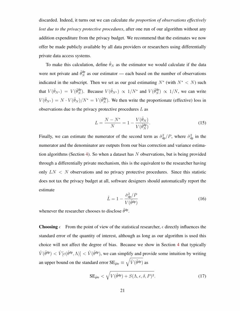
discarded. Indeed, it turns out we can calculate the proportion of observations effectively

lost due to the privacy protective procedures, after one run of our algorithm without any

addition expenditure from the privacy budget. We recommend that the estimates we now

offer be made publicly available by all data providers or researchers using differentially

private data access systems.

To make this calculation, define θN as the estimator we would calculate if the data

were not private and θdpN as our estimator — each based on the number of observations

indicated in the subscript. Then we set as our goal estimating N∗ (with N∗ < N ) such

that V (θN∗) = V (θdpN ). Because V (θN∗) ∝ 1/N∗ and V (θdp

N ) ∝ 1/N , we can write

V (θN∗) = N · V (θN)/N∗ = V (θdpN ). We then write the proportionate (effective) loss in

observations due to the privacy protective procedures L as

L =N −N∗

N= 1− V (θN)

V (θdpN ). (15)

Finally, we can estimate the numerator of the second term as σ2dp/P , where σ2

dp in the

numerator and the denominator are outputs from our bias correction and variance estima-

tion algorithms (Section 4). So when a dataset has N observations, but is being provided

through a differentially private mechanism, this is the equivalent to the researcher having

only LN < N observations and no privacy protective procedures. Since this statistic

does not tax the privacy budget at all, software designers should automatically report the

estimate

L = 1−σ2

dp/P

V (θdp)(16)

whenever the researcher chooses to disclose θdp.

Choosing ε From the point of view of the statistical researcher, ε directly influences the

standard error of the quantity of interest, although as long as our algorithm is used this

choice will not affect the degree of bias. Because we show in Section 4 that typically

V (θdp) < V [c(θdp,Λ)] < V (θdp), we can simplify and provide some intuition by writing

an upper bound on the standard error SEθdp ≡√V (θdp) as

SEθdp <

√V (θdp) + S(Λ, ε, δ, P )2. (17)

21

A researcher can use this expression to judge how much of their allocation of ε to assign

to the next run by using their prior information about the likely value of V (θdp) (as they

would in a power calculation), plugging in the chosen values of Λ, δ and P , and then

trying different values of ε.

Choosing Λ Although our bias correction procedure makes the particular choice of Λ

less consequential, researchers with extra knowledge should use it. In particular, reducing

Λ increases the chance of censoring while reducing noise, while larger values will reduce

censoring but increase noise. This Heisenberg-like property is an intentional feature of

differential privacy, designed to keep researchers from being able to see with too much

precision.

We can however choose among the unbiased estimators our method produces that have

the smallest variance. To do that, researchers should set Λ by trying to capture the point

estimate of the mean. Although this cannot be done with certainty, researchers can often

do this without seeing the data. For example, consider the absolute value of coefficients

from any real application of logistic regression. Although technically unbounded, em-

pirical regularities in how researchers typically scale their input variables lead to logistic

regression coefficients reported in the literature rarely having absolute values above about

five. Similar patterns are easy to identify across many other statistical procedures. A good

software interface would thus not only include appropriate defaults but also enable users

to enter asymmetric Λ intervals, as we do by reparameterization for α2 in Section 4.1.

Then the software, rather than the user, could take responsibility (in the background) for

rescaling the variables as necessary.

Applied researchers are good at making choices like this as they have considerable ex-

perience with scaling variables, a task that is an essential part of most data analyses. Re-

searchers also frequently predict the values of their quantities of interest both informally,

when deciding what analysis to run next, and formally for power calculations. Statis-

ticians and methodologists find it useful to standardize variables and use other similar

techniques to enable them to ignore the substantive features of a problem, but in practice

making data analyses invariant to the substance makes no sense for the researcher seeking

22

to learn something about the world, which is their purpose for conducting the analysis in

the first place. If the data surprise us, we will learn this because the αdp1 and αdp

2 are dis-

closed as part of our procedure. If either quantity is more than about 60%, we recommend

researchers adjust Λ and rerun their analysis (see Appendix B for details).

Practical Implementation Choices As with all policies, privacy policies can be in-

formed by science but not determined by it. Policy choices are by definition always in-

herently political to some degree. This tension is revealed in the privacy literature by

the sometimes divergent perspectives of theorists and practitioners. Theorists tend to

be highly conservative in setting privacy parameters and budgets; practitioners respon-

sible for implementing data access systems usually take a more lenient perspective. Both

perspectives make sense: Theorists analyze worst case scenarios using mathematical cer-

tainty as the standard of proof, and must be ever wary of scientific adversaries hunting for

loopholes in their proposed privacy protective mechanisms. This divergence even makes

sense both theoretically, because privacy bounds are orders of magnitude higher than what

we would expect in practice (Erlingsson, Mironov, et al., 2019), and empirically, because

those responsible for implementing data access systems have little choice but to make

some compromises in turning mathematical proofs into physical reality. In fact, we have

been unable to find even a single large scale implementation of differential privacy that

exactly meets the mathematical standard, even when theorists have been heavily involved

in its design. In practice, common implementations of differential privacy allow larger

values of ε for each run (such as in the single digits), reset the privacy budget each day, or

do not have a privacy budget at all.

We thus offer here two ways of thinking about practical approaches to the use of this

technology. First, although the data sharing regime can be broken by intentional attack,

because we now know that re-identification from de-identified data is often possible, de-

identification is still helpful — not for the ε bound but for reducing risk in practice. It is no

surprise that university Institutional Review Boards have rephrased their regulations from

“de-identified” to “not readily identifiable” rather than responding to recent discoveries

by disallowing data sharing entirely. Indeed, the long history of the data sharing regime

23

has seen exceptionally few instances where a research subject in an academic study was

harmed by unauthorized re-identification (i.e., excluding computer science demonstra-

tions), and so this technology is clearly still of considerable practical use. By adding

some amount of privacy protective procedures, like noise and censoring, to de-identified

data means we are further obscuring and therefore protecting private information. If the

privacy budget is kept small, nothing else need be done, but if we relax this requirement

and allow ε to be larger for any one run we will still be greatly reducing the probability of

privacy violations in practice. In these situations, taking other practical steps is prudent

as well such as disallowing repeated runs of the same analysis (say by returning cached

results).

Second, potential data providers and regulators should ask themselves Are these re-

searchers trustworthy? In the past, they almost always have been, as legitimate academics

have rarely if ever used their access to sensitive data to violate the privacy of their research

subjects. When this fact provides insufficient reassurance for policymakers, we can move

to the data access regime. However, a middle ground does exist by trusting researchers

(perhaps along with auxiliary protections, such as signed data use agreements by univer-

sity employers, financial or career sanctions for violations, and full auditing of all analyses

to verify compliance). With trust, researchers can be given full access to the data, be al-

lowed to run as many analyses of whatever type they wish, but be required to use the

algorithm proposed here for any results to be disclosed publicly. The data holder would

then maintain a strict privacy budget summed over all published analyses, which is far

more useful for scientific research than counting every exploratory data analysis run (but

not necessarily disclosed publicly) against the budget. This plan may in some respects ap-

proximate the differential privacy ideal more closely than the typical data access regime,

as the privacy protections among results published are then completely protected by the

mathematical guarantees. There are theoretical risks (Dwork and Ullman, 2018), but the

advantages to the public good that can come from research with fewer constraints may

also be substantial.

24

Software Design We recommend data access systems that use our procedures allow a

wide range of both statistical methods and quantities of interest calculated from them.

Researchers should be able to choose any quantity (corresponding to θ in our algorithm)

to estimate and disclose. Most of the time, researchers will wish to disclose quantities

derived from statistical models rather than coefficients or other statistics typically output

from statistical software. Statistical researchers view these as valuable for interpreting

the data analysis, but ultimately intermediate quantities on the way to their ultimate quan-

tity of interest. Given the limited privacy budget, researchers will want to choose which

quantities to disclose much more selectively. For example, instead of logit coefficients, re-

searchers would typically be more interested in reporting relative risks, probabilities, and

risk differences (King, Tomz, and Wittenberg, 2000; King and Zeng, 2002). Even regres-

sion coefficients are often best replaced by the exact quantity of interest to the researcher,

such as a predicted value, the probability that one party’s candidate wins the election, or

a first difference. Professional software should also allow researchers to submit statistical

code to be checked and included, since the algorithm we present here can wrap around

any legitimate statistical procedure.

Designing the software user interface to encourage best statistical practices can be

especially valuable. This is especially so for users previously unfamiliar with differen-

tial privacy, whether they are statistically oriented or not. One simple procedure would

be to always provide a simulated dataset (constructed so as not to leak any privacy from

the real dataset) so users could compare the results from runs with and without the pri-

vacy protections and get a feel for how to do data analysis within a differential privacy

framework.

Finally, under the topic of “do not try this at home,” data providers should understand

that a differentially private data access system involves details of implementation not cov-

ered here. These include issues regarding random number generators, privacy budgets,

parallelization, security, authentication, and authorization. They also involve avoiding

side attacks on the timing of the algorithm, statistical methods that occasionally fail (e.g.,

due to collinearity in regression or, in logit, perfect discrimination), the privacy budget,

25

and the state of the computer system (e.g., Garfinkel, Abowd, and Powazek, 2018; Hae-

berlen, Pierce, and Narayan, 2011).

7 Concluding Remarks

The differential privacy literature focuses appropriately on the utility-privacy trade off.

We propose to revise the definition of “utility” for at least some purposes so it offers value

to researchers and others that seek to use confidential data to learn about the world, be-

yond inferences to the inaccessible private data. A scientific statement is not one that is

necessarily correct, but one that comes with known statistical properties and an honest as-

sessment of uncertainty. Utility to scholarly researchers involves inferential validity, the

ability to give these informative scientific statements about populations beyond available

(private or public) data. While differential privacy can guarantee privacy to individuals,

researchers also need inferential validity to make a data access system safe for making

proper scientific statements, for society using the results of that research, and for individ-

uals whose privacy must be protected.

Although our goal here is a generic method, with an estimator that is approximately

unbiased and applicable to a single quantity of interest at a time, more specific meth-

ods, with other properties, would be worth attention from future researchers. Inferential

validity without differential privacy may mean beautiful theory without data access, but

differential privacy without inferential validity may result in biased substantive conclu-

sions that mislead researchers and society at large.

Together, approaches that are differentially private and inferentially valid may begin

to convince companies, governments, and others to let researchers access their unprece-

dented storehouses of informative data about individuals and societies. If this happens, it

will generate guarantees of privacy for individuals, scholarly results for researchers, and

substantial value for society at large.

26

Appendix A Variance Estimation Derivations

We decompose the two variance parameters using the results following Equation 10. The

first we write as V (θdp) = V (θ) + S2θ, where V (θ) is the variance of the mean over P

draws from a normal censored at [−Λ,Λ] (divided by P ), and S2θ

is the variance of the

differentially private noise. The distribution from which this variance is calculated then is

a three component mixture (see Equation 12). The first component is a truncated normal

with mean θT , and bounds [−Λ,Λ]; the two other components are the spikes at Λ and−Λ.

Begin with the following generic formula for the variance of the mean of draws from a

3-component mixture distribution with weights wi, and component mean and variances of

E[θi], σ2i respectively:

V (θ) =1

P·

([3∑i=1

wi(E[θi]2 + σ2

i )

]− E[θ]2

)(18)

with weights w = [(1 − α1 − α2), α2, α1], and with means for the spikes at E[θ2] = Λ,

and E[θ3] = −Λ and variances σ22 = σ2

3 = 0. Then, rearranging Equation 12, we write

the truncated normal mean as

E[θ1] ≡ θT =E[θ]− Λ(α1 + α2)

1− α2 − α1

. (19)

and we express the variance of the truncated normal as

σ21 = σ2

[1 +

(−Λ−θσ

)Q1 −

(Λ−θσ

)Q2

1− α2 − α1

−(

Q1 −Q2

1− α2 − α1

)2]

(20)

where Q1 = 1√2π

exp(−1

2

(−Λ−θσ

)2)

and Q2 = 1√2π

exp(−1

2

(Λ−θσ

)2)

. σ2 is the variance

of the distribution from which partitions are drawn (before censoring).

We now use these results to fill in Equation 18:

V (θ) =1

P·(

(1− α2 − α1)(θT + σ2

1

)+ Λ2(α2 + α1)− E[θ]2

). (21)

Finally, our estimator of this variance simply involves plugging in for {α1, α2, θdp, σdp, θdp}

the values {α1, α2, θ, σ, E[θ]}, respectively.

Next, we decompose the second parameter of the variance matrix of Equation 14 in

the same way: V (αdp2 ) = V (α2) + S2

α, the first component of which is the variance of the

27

proportion of partitions that are censored (prior to adding noise). We represent whether a

partition is censored or not by an indicator variable equal to 1 with probability α2: IfAp =

1(θp > Λ), then Pr(Ap = 1) = α2. Then the sum of iid binary variables is a binomial,

with variance V(∑P

p=1Ap

)= Pα2(1−α2). Plugging αdp

2 into the decomposition yields

V (α) =1

P(1− αdp

2 )αdp2 + S2

α. (22)

Finally, we derive the covariance:

Cov(θdp, αdp2 ) = Cov(θ, α2) (noise is additive and independent)

= Cov

(1

P

P∑p=1

c(θp,Λ),1

P

P∑p=1

Ap

)

=1

PCov

(c(θ1,Λ), A1

)(θp and Ap are iid over p)

=1

P

{E[c(θ1,Λ)A1]− E[c(θ1,Λ)E(A1)]

}=

1

P

{E[c(θ1,Λ) | A1 = 1)− E[c(θ1,Λ) | A1 = 0]

}α2(1− α2) (23)

where E[c(θ1,Λ) | A1 = 1] = Λ, and E[c(θ1,Λ) | A1 = 0] = θT , the mean of the

truncated normal mean component of the censored normal. We thus use Equation 19 and

plug estimates into Equation 23:

Cov(θdp, αdp2 ) =

1

P

(Λ− θdp − α2Λ + α1Λ

1− α2 − α1

)α2(1− α2). (24)

Appendix B When Privacy Procedures Obscure All Rel-evant Information

All privacy protective procedures are designed to destroy or hide information by making it

more difficult to draw certain inferences from confidential data. These are worthwhile to

protect individual privacy and to ensure that data which might not otherwise be accessible

at all are in fact available to researchers. However, with the noise and censoring used in

differential privacy, some inferences will be so uncertain that no substantive knowledge

can be learned. In even more extreme situations, our bias correction procedures, which

rely on some information passing through the differential privacy filters, would have no

28

leverage left to do their work. In this appendix, we develop a rule of thumb that sug-

gests when privacy protected data analysis becomes like trying to get blood from a stone:

max(α1, α2) > 0.6 or εP < 100 (also, if εP � 100 then max(α1, α2) could be even

larger before a problem occurs). If an analysis is implicated by this rule of thumb, then

it is best to rerun the analysis with more partitions, use more of the privacy budget, or

adjust Λ. If none of these are possible, then the only options are to negotiate with the data

provider for a larger privacy budget allocation, collect more data, or abandon inquiry into

this particular quantity of interest.

Recall that we attempt to choose Λ in order that each θp ∈ [−Λ,Λ]. We then keep this

interval fixed and study the distribution of the mean θ = 1P

∑Pp=1 θp, which has a variance

P times smaller than the distribution of θp. Now consider the unusual edge case where

so much noise is added that |θdp| � Λ (in contrast to a small deviation, which has little

consequence). In this extreme situation, using θdp as a plug-in estimator for E(θdp) no

longer works because no values of θ and σ2 can be logically consistent with it, given Λ;

in some ways, such a result even nonsensically suggests that σ2 < 0.

In this situation, we could simply stop and declare that no reasonable inference is

possible and, if we do, we wind up with an analogous rule of thumb. However, to build

intuition for this rule, we now show what happens if we try to accommodate this edge

case computationally. Thus, if θdp > Λ we learn that e > 0 (where e is the differentially

private error defined in Equations 7-8), and so we replace θdp with θdp ≡ θdp−S√

2√π

, where

the second term is E(e|θdp > Λ) = E(e|e > 0). This adjustment makes the system of

equations (and the resulting θdp) possible, at the cost of some (third order) bias. We now

derive our rule of thumb by showing how to bound this bias by appropriately choosing ε,

P , and Λ.

For simplicity, we study the dominant case of one-sided censoring (α1 = 0), which

enables us to solve the bias correction equations algebraically rather than numerically; the

results are not very different for two-sided censoring. Thus, begin with the facts, including

29

α2 in Equation 11 and

θdp = (1− αdp2 )

θ −σ√2π

exp

(−1

2

(Λ−θdp

σ

)2)

(1− αdp2 )

+ αdp2 Λ. (25)

Then solve these equations for θ, which we label θdp as above, and show, conditional on

α2, that θdp is a linear function of θdp:

θdp = θdp(

1

B

)+ Λ

(B − 1

B

), (26)

where B = (1− αdp2 ) +

√2e−T2/2

2T√π

and T =√

2 · erf−1[2(1− αdp2 )− 1].

Note that if we apply our bias correction (in Section 4.1) using the exact version of

E(θ) (and α2) as an input, we would find θdp = θ. We are therefore interested in the

discrepancy d = E(θdp)− E(θ), which we write as

d =

[(1− Pr(θdp > Λ))

∫ Λ

−∞

tN (t|θ, S2)

(1− Pr(θdp > Λ))dt

+ Pr(θdp > Λ)

∫ ∞Λ

(t− S

√2√π

)N (t|θ, S2)

Pr(θdp > Λ)dt

]− E[θ]

=

[E[θdp]− Pr(θdp > Λ)S

√2√π

]− E[θ]

=− S√

2√π× Pr(θdp > Λ)

=−2Λ√

2 ln(1.25/δ)

εP

√2√π× Pr(θdp > Λ), (27)

where Pr(θdp > Λ) =∫∞

ΛN (t|θ, S2)dt has a maximum value of 0.5. As a result, the

maximum value of the discrepancy is

max(d) = −2Λ√

ln(1.25/δ)/π

εP. (28)

Making use of Equation 26, we write the maximum possible bias in θdp as a function

of the maximum possible bias in θdp. Thus,

E[θdp]− θ ≤(

1

B

)·max(d) (29)

which shows that the bias depends on 1/B, which itself is a deterministic function of α2.

30

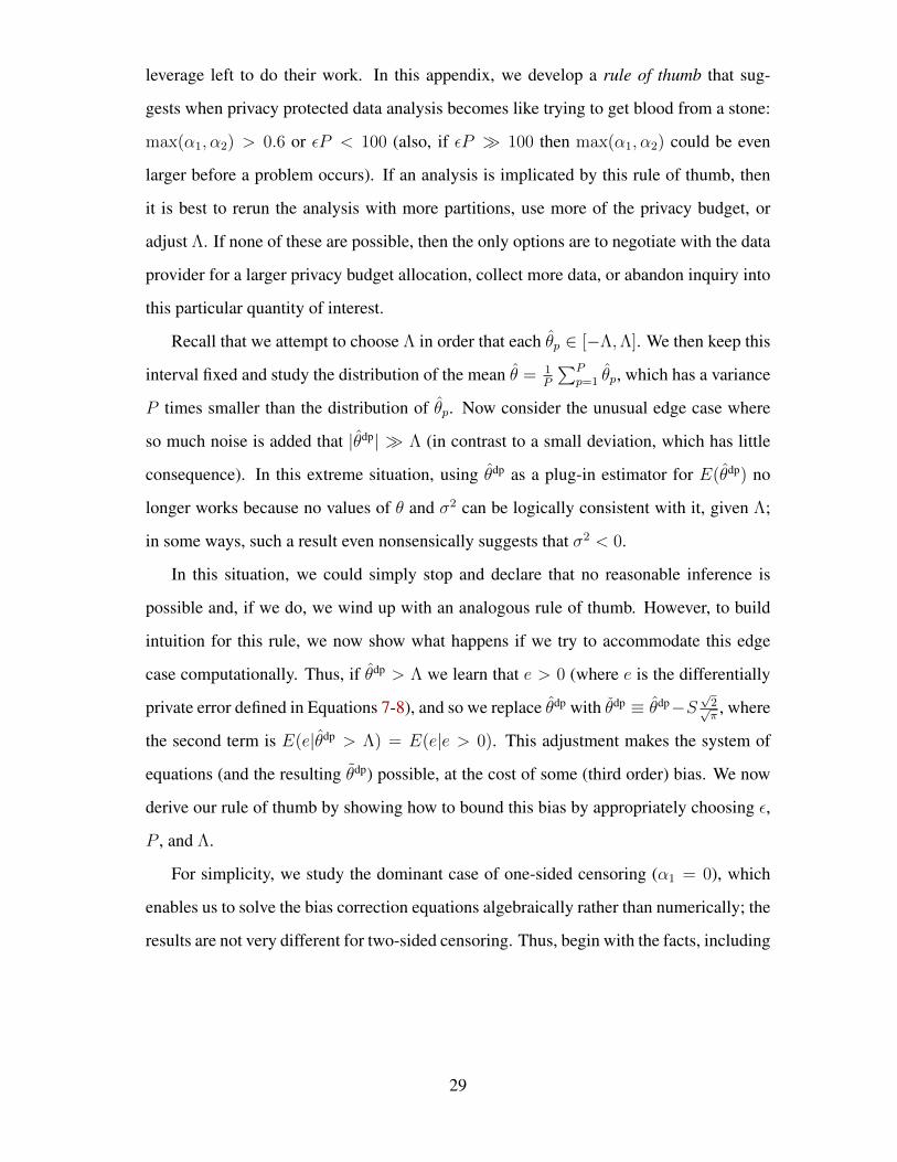
As shown in Figure 3, which plots this relationship, if censoring (plotted horizontally)

is 0.5, then θdp is unbiased. We also see that we can control the maximum value of 1/B by

controlling the level of censoring. If we follow our rule of thumb and disallow censoring

over 60%, then max0≤α2≤0.6 | 1B | = 1.

0

2

4

6

0.0 0.2 0.4 0.6 0.8α2

|1/B

|

Figure 3: Relationship between |1/B| and Percent Censored

To find the maximum bias under this decision rule, note that if Pr(θdp > Λ) is at its

maximum, then α2 = 0.5 and 1/B → 0. It follows that 1B

Pr(θdp > Λ) is strictly less than

0.5 and we are able to bound the absolute value of the discrepancy:

|E(θdp)− θ| <

∣∣∣∣∣2Λ√

ln(1.25/δ)/π

εP

∣∣∣∣∣ . (30)

We use this result to show that we have approximately bounded the bias in θdp (if the

computational fix is applied) relative to our quantity of interest θ. Since users set Λ on the

scale of their quantity of interest to the range [−Λ,Λ], the maximum proportionate bias is

less than approximately

1

Λ

∣∣∣∣∣2Λ√

ln(1.25/δ)π

εP

∣∣∣∣∣ =

∣∣∣∣∣2√

ln(1.25/δ)π

εP

∣∣∣∣∣ . (31)

For example, if we choose, from our rule of thumb, εP = 100 and δ = 0.01, then this

evaluates to 0.03, a small proportionate bias. Of course, this is the upper bound; the actual

bias is likely to be a good deal smaller than even this small bound in most applications.

31

ReferencesBalle, Borja and Yu-Xiang Wang (2018): “Improving the gaussian mechanism for dif-

ferential privacy: Analytical calibration and optimal denoising”. In: arXiv preprintarXiv:1805.06530.

Barrientos, Andrés F., Jerome Reiter, Machanavajjhala Ashwin, and Yan Chen (July 2019):“Differentially Private Significance Tests for Regression Coefficients”. In: Journal ofComputational and Graphical Statistics, pp. 1–24.

Blackwell, Matthew, James Honaker, and Gary King (2017): “A Unified Approach toMeasurement Error and Missing Data: Overview”. In: Sociological Methods and Re-search, no. 3, vol. 46, pp. 303–341.

Blair, Graeme, Kosuke Imai, and Yang-Yang Zhou (2015): “Design and analysis of therandomized response technique”. In: Journal of the American Statistical Association,no. 511, vol. 110, pp. 1304–1319.

Bun, Mark and Thomas Steinke (2016): “Concentrated differential privacy: Simplifica-tions, extensions, and lower bounds”. In: Theory of Cryptography Conference. Springer,pp. 635–658.

Carlini, Nicholas, Chang Liu, Úlfar Erlingsson, Jernej Kos, and Dawn Song (2019): “TheSecret Sharer: Evaluating and testing unintended memorization in neural networks”.In: 28th {USENIX} Security Symposium ({USENIX} Security 19), pp. 267–284.

Desfontaines, Damien and Balázs Pejó (2019): “SoK: Differential Privacies”. In: CoRR,vol. abs/1906.01337. arXiv: 1906.01337. URL: http://arxiv.org/abs/1906.01337.

Ding, Bolin, Janardhan Kulkarni, and Sergey Yekhanin (2017): “Collecting telemetry dataprivately”. In: Advances in Neural Information Processing Systems, pp. 3571–3580.

Dwork, Cynthia, Vitaly Feldman, Moritz Hardt, Toniann Pitassi, Omer Reingold, andAaron Roth (2015): “The reusable holdout: Preserving validity in adaptive data anal-ysis”. In: Science, no. 6248, vol. 349, pp. 636–638.

Dwork, Cynthia, Frank McSherry, Kobbi Nissim, and Adam Smith (2006): “Calibratingnoise to sensitivity in private data analysis”. In: Theory of cryptography conference.Springer, pp. 265–284.

Dwork, Cynthia and Aaron Roth (2014): “The algorithmic foundations of differential pri-vacy”. In: Foundations and Trends in Theoretical Computer Science, no. 3–4, vol. 9,pp. 211–407.

Dwork, Cynthia and Jonathan Ullman (2018): “The fienberg problem: How to allow hu-man interactive data analysis in the age of differential privacy”. In: Journal of Privacyand Confidentiality, no. 1, vol. 8.

Erlingsson, Úlfar, Ilya Mironov, Ananth Raghunathan, and Shuang Song (2019): “Thatwhich we call private”. In: arXiv preprint arXiv:1908.03566.

Erlingsson, Úlfar, Vasyl Pihur, and Aleksandra Korolova (2014): “RAPPOR: Randomizedaggregatable privacy-preserving ordinal response”. In: Proceedings of the 2014 ACMSIGSAC conference on computer and communications security. ACM, pp. 1054–1067.

Gaboardi, Marco, Hyun-Woo Lim, Ryan M Rogers, and Salil P Vadhan (2016): “Dif-ferentially private chi-squared hypothesis testing: Goodness of fit and independencetesting”. In: ICML’16 Proceedings of the 33rd International Conference on Interna-tional Conference on Machine Learning-Volume 48. JMLR.

32

Garfinkel, Simson L, John M Abowd, and Sarah Powazek (2018): “Issues encountereddeploying differential privacy”. In: Proceedings of the 2018 Workshop on Privacy inthe Electronic Society. ACM, pp. 133–137.

Glynn, Adam N (2013): “What can we learn with statistical truth serum? Design andanalysis of the list experiment”. In: Public Opinion Quarterly, no. S1, vol. 77, pp. 159–172.

Guess, Andrew, Jonathan Nagler, and Joshua Tucker (2019): “Less than you think: Preva-lence and predictors of fake news dissemination on Facebook”. In: Science advances,no. 1, vol. 5, eaau4586.

Haeberlen, Andreas, Benjamin C Pierce, and Arjun Narayan (2011): “Differential PrivacyUnder Fire.” In: USENIX Security Symposium.

Jayaraman, Bargav and David Evans (2019): “Evaluating Differentially Private MachineLearning in Practice”. In: 28th USENIX Security Symposium (USENIX Security 19).Santa Clara, CA: USENIX Association.

Karwa, Vishesh and Salil Vadhan (2017): “Finite sample differentially private confidenceintervals”. In: arXiv preprint arXiv:1711.03908.

King, Gary, Robert O. Keohane, and Sidney Verba (1994): Designing Social Inquiry:Scientific Inference in Qualitative Research. Princeton: Princeton University Press.URL: bit.ly/gKroKsV.

King, Gary and Nathaniel Persily (In press): “A New Model for Industry-Academic Part-nerships”. In: PS: Political Science and Politics. URL: GaryKing.org/partnerships.

King, Gary, Michael Tomz, and Jason Wittenberg (Apr. 2000): “Making the Most of Sta-tistical Analyses: Improving Interpretation and Presentation”. In: American Journal ofPolitical Science, no. 2, vol. 44, pp. 341–355. URL: bit.ly/makemost.

King, Gary and Langche Zeng (2002): “Estimating Risk and Rate Levels, Ratios, andDifferences in Case-Control Studies”. In: Statistics in Medicine, vol. 21, pp. 1409–1427. URL: bit.ly/estrrCC.

Kleiner, Ariel, Ameet Talwalkar, Purnamrita Sarkar, and Michael I Jordan (2014): “Ascalable bootstrap for massive data”. In: Journal of the Royal Statistical Society: SeriesB (Statistical Methodology), no. 4, vol. 76, pp. 795–816.

Mironov, Ilya (2017): “Rényi differential privacy”. In: 2017 IEEE 30th Computer SecurityFoundations Symposium (CSF). IEEE, pp. 263–275.

Mohan, Prashanth, Abhradeep Thakurta, Elaine Shi, Dawn Song, and David Culler (2012):“GUPT: privacy preserving data analysis made easy”. In: Proceedings of the 2012ACM SIGMOD International Conference on Management of Data, pp. 349–360.

Monogan, James E (2015): “Research preregistration in political science: The case, coun-terarguments, and a response to critiques”. In: PS: Political Science & Politics, no. 3,vol. 48, pp. 425–429.

Nissim, Kobbi, Sofya Raskhodnikova, and Adam Smith (2007): “Smooth sensitivity andsampling in private data analysis”. In: Proceedings of the thirty-ninth annual ACMsymposium on Theory of computing. ACM, pp. 75–84.

Politis, Dimitris N, Joseph P Romano, and Michael Wolf (1999): Subsampling. SpringerScience & Business Media.

Roberts, Margaret E (2018): Censored: distraction and diversion inside China’s GreatFirewall. Princeton University Press.

33

Sheffet, Or (2017): “Differentially private ordinary least squares”. In: Proceedings of the34th International Conference on Machine Learning-Volume 70, pp. 3105–3114.

Smith, Adam (2011): “Privacy-preserving statistical estimation with optimal convergencerates”. In: Proceedings of the forty-third annual ACM symposium on Theory of com-puting. ACM, pp. 813–822.

Stefanski, L. A. (2000): “Measurement Error Models”. In: Journal of the American Sta-tistical Association, no. 452, vol. 95, pp. 1353–1358.

Sweeney, Latanya (1997): “Weaving technology and policy together to maintain confi-dentiality”. In: The Journal of Law, Medicine & Ethics, no. 2-3, vol. 25, pp. 98–110.

Tang, Jun, Aleksandra Korolova, Xiaolong Bai, Xueqiang Wang, and Xiaofeng Wang(2017): “Privacy loss in apple’s implementation of differential privacy on macos 10.12”.In: arXiv preprint arXiv:1709.02753.

Vadhan, Salil (2017): “The complexity of differential privacy”. In: Tutorials on the Foun-dations of Cryptography. Springer, pp. 347–450.

Wang, Yue, Daniel Kifer, and Jaewoo Lee (2018): “Differentially Private Confidence In-tervals for Empirical Risk Minimization”. In: arXiv preprint arXiv:1804.03794.

Wang, Yue, Jaewoo Lee, and Daniel Kifer (2015): “Differentially private hypothesis test-ing, revisited”. In: arXiv preprint arXiv:1511.03376, vol. 1.

Warner, Stanley L (1965): “Randomized response: A survey technique for eliminatingevasive answer bias”. In: Journal of the American Statistical Association, no. 309,vol. 60, pp. 63–69.

Wasserman, Larry (2006): All of nonparametric statistics. Springer Science & BusinessMedia.

— (2012): “Minimaxity, statistical thinking and differential privacy”. In: Journal of Pri-vacy and Confidentiality, no. 1, vol. 4.

Williams, Oliver and Frank McSherry (2010): “Probabilistic inference and differentialprivacy”. In: Advances in Neural Information Processing Systems, pp. 2451–2459.

Wilson, Royce J, Celia Yuxin Zhang, William Lam, Damien Desfontaines, Daniel Simmons-Marengo, and Bryant Gipson (2019): “Differentially Private SQL with Bounded UserContribution”. In: arXiv preprint arXiv:1909.01917.

Winship, Christopher and Robert D. Mare (1992): “Models for Sample Selection Bias”.In: Annual Review of Sociology, vol. 18, pp. 327–50.

Wood, Alexandra, Micah Altman, Aaron Bembenek, Mark Bun, Marco Gaboardi, JamesHonaker, Kobbi Nissim, David R O’Brien, Thomas Steinke, and Salil Vadhan (2018):“Differential Privacy: A Primer for a Non-Technical Audience”. In: Vand. J. Ent. &Tech. L. Vol. 21, p. 209.

34