Device-independent randomness generationfrom several Bell estimators

Olmo Nieto-Silleras, Cédric Bamps, Jonathan Silman, Stefano Pironio

Laboratoire d’Information Quantique, CP224Université libre de Bruxelles, 1050 Brussels (Belgium)

(Dated: March 20, 2018)

AbstractDevice-independent randomness generation and quantum key distribution protocols rely on a

fundamental relation between the non-locality of quantum theory and its random character. Thisrelation is usually expressed in terms of a trade-off between the probability of guessing correctlythe outcomes of measurements performed on quantum systems and the amount of violation of agiven Bell inequality. However, a more accurate assessment of the randomness produced in Bellexperiments can be obtained if the value of several Bell expressions is simultaneously taken intoaccount, or if the full set of probabilities characterizing the behavior of the device is considered.We introduce protocols for device-independent randomness generation, secure against classical sideinformation, that rely on the estimation of an arbitrary number of Bell expressions or even directlyon the experimental frequencies of measurement outcomes. Asymptotically, this results in an optimalgeneration of randomness from experimental data (as measured by the min-entropy), without havingto assume beforehand that the devices violate a specific Bell inequality.

1 IntroductionIn recent years, researchers have uncovered a fundamental relationship between the non-locality of quan-tum theory and its random character. This relationship is usually formulated as follows. Consider two(or generally k) separated quantum devices accepting, respectively, classical inputs x1 and x2 and out-putting classical outputs a1 and a2. Let p = p(a1a2 |x1x2) denote the set of joint probabilities describinghow the devices respond to given inputs, from the point of view of a user who can only interact withthe devices through the input-output interface, but who has no knowledge of the inner workings of thedevices. Suppose that given p, the expectation value of a certain Bell expression f , such as the Clauser-Horne-Shimony-Holt (CHSH) expression [1], equals f [p]. Then, it is in principle possible to compute alower bound on the randomness generated by the devices, as quantified by the min-entropy—the negativelogarithm of the maximal probability of correctly guessing the values of future outputs. This bound onthe min-entropy holds for any observer, including those having an arbitrarily precise description of theinner workings of the devices, and depends only on information derived from the resulting input-outputbehavior through the quantity f [p]. In principle, this bound can be computed numerically for any givenBell expression f . For certain Bell expressions, such as the CHSH expression, it can also be determinedanalytically.

This relation between the non-locality of quantum theory and its randomness is at the basis of variousprotocols for device-independent (DI) randomness generation (RNG) [2, 3] and quantum key distribution(QKD) [4, 5]. The theoretical analysis of such protocols presents us with an extra challenge in that theprobabilistic behavior p of the devices is not known in advance and may vary from one measurementrun to the next. This implies that bounds on the randomness as a function of f [p] have to be adaptedto rely instead on the value of the Bell expression f estimated from experimental data. Some DIRNGand DIQKD protocols, and their security analyses, are reliant on specific Bell inequalities (usually theCHSH inequality) [6–9] or certain families of Bell inequalities [10–12], while others may be adapted to

1

arX

iv:1

611.

0035

2v4

[qu

ant-

ph]

19

Mar

201

8

arbitrary Bell inequalities [3, 13–17]. However, to our knowledge all DIRNG and DIQKD protocols inthe literature require that a single Bell inequality be chosen in advance and its experimental violationestimated (one exception is [18], where two fixed Bell expressions are used). The length and secrecy ofthe final key will then depend on the observed violation of the chosen inequality.

Nevertheless, it has been pointed out in [19, 20] that the fundamental relation between the randomnessand non-locality of quantum theory does not necessarily need to be expressed in terms of a specificBell inequality. It is in principle possible, at least numerically, to bound the probability of guessingcorrectly the outputs of a pair of quantum devices directly from the knowledge of the joint input-outputprobabilities p. Indeed, the amount of violation f [p] of a given Bell inequality captures the non-localbehavior of the devices only partially, and better bounds on the min-entropy can be obtained if all theinformation about the devices’ behavior is taken into account.

This observation raises the following question: can one devise a device-independent RNG or QKDprotocol that does not rely on the estimation of any a priori chosen Bell inequality, but which insteadtakes directly into account all the data generated by the devices?

There are various reasons for introducing protocols of this type. First, as already mentioned, theentire set of data generated by the devices can provide more information than the violation of a specificBell inequality, and may therefore potentially allow for more efficient protocols. Second, the choice of aBell inequality may have a deep influence on the amount of randomness that can be certified: as shownin [21] there are devices for which the amount of randomness, as computed from the CHSH inequality,is arbitrarily small, but is maximal if computed using another Bell inequality. Third, even if a set ofquantum devices have been specifically designed to maximize the randomness according to a specificBell inequality, the optimal extraction of randomness from noisy versions of such devices, say because ofdegradation of the devices with time, will typically rely on other Bell inequalities [19, 20, 22]. Finally,suppose that one is given a set of quantum devices without any specification of which Bell inequalitythey are expected to violate. Can one nevertheless directly use them in a protocol and obtain a non-zerorandom string or shared key, without testing their behavior beforehand?

We show here that it is indeed possible to devise DIRNG protocols which exploit more informationthan the estimated violation of a single Bell inequality, particularly, DIRNG protocols which exploit thefull set of frequencies obtained (i.e., the entire set of estimates of the behavior p). Specifically, we intro-duce a DIRNG protocol whose security holds against an adversary limited to classical side information,or equivalently, with no long-term quantum memory. (Note that such a level of security may well besufficient for all practical purposes [14, 15].) Technically, our protocol is obtained by generalizing thesecurity analysis introduced in [14, 15] and combining it with the semidefinite programming techniquesintroduced in [19, 20] for lower-bounding the randomness based on the full set of probabilities p (whichcannot be directly applied to experimental data).

We start in Section 2 by briefly presenting the theoretical framework of our work, its main assump-tions, and the notation used throughout the paper. In Sections 3 to 5 we present our main mathematicalresults. In Section 3 we present the main theorem of the paper and explain in detail how to put a DIbound on the randomness produced when measuring a Bell device n times in succession, given that wehave a way to bound the single-round randomness as a function of the Bell expectation, and given thatwe can estimate the Bell expectation with some confidence. These two sub-procedures are respectivelypresented in Sections 4 and 5 for the general case of an arbitrary number of Bell expressions. Combiningthese two sub-procedures with the general approach of Section 3 immediately yields a DIRNG protocol,whose various steps are summarized in Section 6. In Section 7 we discuss in detail the main features ofour protocol, and illustrate these with a numerical example. We end with some concluding remarks andopen questions in Section 8.

2 Behaviors and Bell expressionsIn the following we will refer to a Bell set up, that is to say, k separated “black” boxes (quantum deviceswhose inner workings are unknown), as a Bell device. Each box i can receive an input xi upon which itproduces an output ai, with xi and ai taking values in some finite sets Xi and Ai, respectively, wherewithout loss of generality we assume that the set of outputs Ai does not depend on the input xi. We writex = (x1, . . . , xk) and a = (a1, . . . , ak) for the k-tuple of inputs and outputs, and write X = X1× · · · ×Xkand A = A1 × · · · × Ak for the set of all possible k-tuples of inputs and outputs. Note that we use a

2

roman (upright) type for the inputs and outputs of a single box and an italic type for the joint inputsand outputs of all k boxes.

The behavior of a single-round use of this Bell device can be characterized by the |A| × |X | jointprobabilities p(a | x), which we can arrange into a vector p ∈ R|A|×|X|. We denote by Q ⊂ R|A|×|X| theset of behaviors p which admit a quantum representation, i.e., the set of behaviors such that there exista k-partite quantum state and local measurements yielding the outcomes a with probability p(a |x) whenperforming the measurements x. It is well-known that the set Q can be approximated from its exterior(from outside the set) by a series of semidefinite programs (SDP) using the NPA hierarchy [23].

We define a Bell expression as a vector f ∈ R|A|×|X| with components f(a, x). The Bell expressionf defines a linear form on the set of behaviors p through

f [p] =∑a,x

f(a, x)p(a | x) . (1)

We refer to f [p] as the expectation of f with respect to the behavior p.We consider here a framework in which the information we have about a Bell device is not necessarily

given by the full behavior p, but possibly only by the expectation of one or more Bell expressions. In thefollowing, we thus assume that t Bell expressions fα (α = 1, . . . , t) have been selected. (The certifiablerandomness will depend on this initial choice of Bell expressions; we discuss this issue later.) We denoteby f = (f1, . . . , ft) these t Bell expressions and by f [p] = (f1[p], . . . , ft[p]) their expectations with respectto the behavior p. As an example, in a bipartite scenario, we might only know the value of the CHSHexpression, in which case t = 1 and there is a single f defined by f(a, x) = (−1)a1+a2+x1x2 . But theframework is also applicable when f [p] corresponds to the full set p of probabilities. One simply needs toconsider |A|× |X | expressions, one for each pairing (a, x), which are defined by fa,x(a′, x′) = δ(a,x),(a′,x′),so that fa,x[p] = p(a | x).

Of course, in a DI protocol, we are not actually given f [p]; we must instead estimate it by performingsequential measurements. We are thus led to consider a Bell device which is used n times in succession.We write ~x = (x1, . . . , xn) and ~a = (a1, . . . , an) for the corresponding sequence of inputs and outputsand ~xj = (x1, . . . , xj) and ~aj = (a1, . . . , aj) for the sequences of inputs and outputs up to, and including,round j.

We write P (~a | ~x) for the conditional probabilities of obtaining the sequence of outputs ~a given acertain sequence of inputs ~x. Note that we use an upper-case P to denote the n-round behavior of theboxes and lower-case p’s for single-round behaviors. We assume that the Bell device is probed usinginputs ~x distributed according to a probability distribution Π(~x). We will consider, in particular, thecase where at each round the inputs are selected according to identical and independent distributionsπ(x), so that Π(~x) =

∏nj=1 π(xj) (though this condition can actually be slightly relaxed in the results

that follow). The full (non-conditional) n-round probabilities are thus given by P (~a, ~x) = P (~a | ~x) Π(~x).We denote by PAX and PA|X the distributions corresponding to the probabilities P (~a, ~x) and P (~a | ~x),respectively.

The only assumption we make about the Bell device is that at each round it is characterized by ajoint entangled quantum state and a respective set of local measurement operators for each box. Eachset of local measurement operators can depend on the past inputs and outputs of all k boxes (separatedboxes can thus freely communicate between measurement rounds), but does not depend on future inputs(inputs are thus selected independently of the state of the device) or inputs of the k−1 other boxes in thesame round. Mathematically, this means that we can write P (~a | ~x) =

∏nj=1 P (aj | xj ,~aj−1, ~xj−1), and

that the (single-round) behavior at round j given the past inputs and outputs ~xj−1 and ~aj−1, definedas p~aj−1,~xj−1(aj | xj) = P (aj | xj ,~aj−1, ~xj−1), should be a valid no-signaling quantum behavior, i.e.,p~aj−1,~xj−1 ∈ Q.

We assume that the internal behavior of the boxes may be classically correlated with a system heldby an adversary. Formally, these correlations and the adversary’s knowledge can be represented throughthe joint probabilities P (~a, ~x, e), where e denotes the adversary’s classical side information. However, inorder to keep the notation simple, we do not explicitly include e in the following. All the reasonings thatfollow would nevertheless hold, with only minor modifications, if the adversary’s classical side informatione were explicitly taken into account. This can be understood by comparing our proofs with those in [14].Alternatively, e can be formally viewed as an initial input x0 = e.

In the following, we sometimes adopt a terminology where the k-tuples x and a are referred to as the

3

input and output of (a single-round use of) the Bell device (though of course each consists of the inputsand outputs, respectively, of all k boxes).

3 A general procedure for DIRNG against classical side-infor-mation

In this section, we show how to quantify the randomness produced by n sequential uses of the Bell devicebased on the Bell expressions f . We follow the approach introduced in [3, 14]. This approach relies ontwo essential sub-procedures: a first sub-procedure to bound the randomness of single-round behaviorsand a second sub-procedure to estimate a certain quantity involving the Bell expressions f . Given thesetwo ingredients, the single-round randomness bound can, through some simple algebra, be adapted tothe n-round scenario and related to the actual data obtained in the Bell experiment.

We provide a macro-level description of this approach, which relies only on certain general mathe-matical properties that these two basic sub-procedures must satisfy, but not on any specifics as to howto implement them. We will present explicit ways to carry out these sub-procedures in the next twosections.

Intuitively, the output of the Bell device exhibits randomness for some choice of input ~x if there isno corresponding outcome that is certain to happen, i.e., if P (~a | ~x) < 1 for all ~a ∈ An. Equivalently,we can express this condition by saying that the surprisals − log2 P (~a | ~x) are bounded away from zero:− log2 P (~a | ~x) > 0 for all ~a ∈ An. Our first aim will thus be to lower-bound these surprisals withoutmaking any assumptions regarding the Bell device’s behavior apart from the ones stated in Section 2.We will then see how to turn this bound into a more formal statement in terms of min-entropy.

To bound the n-round randomness, we assume the existence of a function H which bounds the single-round surprisal − log2 p(a | x) as a function of the Bell expectations f [p]. This is our first ingredient.We actually require this function to non-trivially bound the surprisals − log2 p(a | x) corresponding to acertain subset Xr ⊆ X of all possible inputs. This is because for certain behaviors, some inputs x lead toless predictable outputs than those resulting from other inputs, and we would therefore prefer to focuson these inputs only. (As will be elaborated on later, the amount of certifiable randomness generallydepends on the choice of Xr.) Formally, the function H, on which our results are based, is defined asfollows.

Definition 1. Let f [Q] = f [p] : p ∈ Q be the set of Bell expectation vectors compatible with at leastone quantum behavior. A function H : f [Q]→ [0, log2 |A|] is a randomness-bounding (RB) function if itsatisfies the following properties:

1. mina∈A,x∈Xr(− log2 p(a | x)

)≥ H(f [p]) for all p ∈ Q.

2. H(f [p]) is a convex function of its argument:

H(q f [p1] + (1− q) f [p2]

)≤ qH(f [p1]) + (1− q)H(f [p2]) (2)

for any 0 ≤ q ≤ 1 and any p1, p2 ∈ Q.

We will also need to compute a lower bound on H(f [p]) for all behaviors p ∈ Q such that f [p] ∈ Vfor some arbitrary region V ⊆ Rt. We thus extend our definition of H to sets, such that

H(V) ≤ infH(f [p]) : f [p] ∈ f [Q] ∩ V . (3)

When f [Q] ∩ V = ∅, we define H(V) = 0. Furthermore, we define η to be a constant such that η ≥η∗ = maxp∈QH(f [p]). (In case η∗ is hard to compute, we may always use η = log2|A|.) We discuss theintuitive interpretation of H and its properties in Section 5.

Given a RB function H, we can now easily lower-bound the n-round surprisals:

Lemma 1. Let H be a RB function. Then, for any (~a, ~x) and any Bell device behavior PA|X

− log2 P (~a | ~x) ≥ nH

1n

n∑j=1

f[p~aj−1,~xj−1

]− ν(~x)η , (4)

4

where

ν(~x) =n∑j=1

1X\Xr (xj) (5)

is the number of xj in ~x = (x1, . . . , xn) which do not belong to the set Xr.

Proof of Lemma 1. The proof follows essentially the same steps as the proof of Lemma 1 in [14]. Themain differences are (a) that we express the bound eq. (4) as a function of t Bell expressions, instead of asingle Bell expression, and (b) that the bound considers explicitly only the randomness from the inputsin Xr.

From our assumptions regarding the Bell device, it follows that for any (~a, ~x) we can write

− log2 P (~a | ~x) = − log2

n∏j=1

p~aj−1,~xj−1(aj | xj) =n∑j=1− log2 p~aj−1,~xj−1(aj | xj). (6)

Each term in the sum such that xj ∈ Xr can be bounded by H(f [p~aj−1,~xj−1 ]) according to the definition ofthe functionH. If xj /∈ Xr, it is certainly the case that − log2 p~aj−1,~xj−1(aj |xj) ≥ 0 ≥ H(f [p~aj−1,~xj−1 ])−η.We can thus write

− log2 P (~a | ~x) ≥n∑j=1

H(f [p~aj−1,~xj−1 ])− ν(~x)η (7)

≥ nH

1n

n∑j=1

f[p~aj−1,~xj−1

]− ν(~x)η, (8)

where in the last line we have exploited the convexity of H.

Lemma 1 tells us how to bound the surprisals − log2 P (~a | ~x) as a function of 1n

∑nj=1 f [p~aj−1,~xj−1 ],

which can be understood as an n-round average Bell expectation, where the average is taken conditionedon past inputs and outputs at each preceding round. This quantity, however, is not directly observable.This leads us to introduce the following definition of a confidence region, which is the second ingredientneeded in our approach.

Definition 2. A 1− ε confidence region V(~a, ~x, ε) for 1n

∑nj=1 f [p~aj−1,~xj−1 ] is a subset of Rt such that,

according to any distribution PAX ,

Pr

1n

n∑j=1

f[p~aj−1,~xj−1

]∈ V(~a, ~x, ε)

≥ 1− ε . (9)

We denote by V = (~a, ~x) : 1n

∑nj=1 f [p~aj−1,~xj−1 ] ∈ V(~a, ~x, ε) the set of input-output sequences such

that 1n

∑nj=1 f [p~aj−1,~xj−1 ] belongs to the confidence region V.

(Note that in general V explicitly depends on ~a and ~x, although notation-wise this dependence is some-times left implicit.) In other words, for small ε and large n, knowing the outcomes (~a, ~x) of n rounds ofmeasurement, one can determine V = V(~a, ~x, ε) and assert with high confidence that 1

n

∑nj=1 f [p~aj−1,~xj−1 ]

is somewhere in V, even though its exact value cannot be deduced from (~a, ~x) alone. The assertion isfalse if and only if (~a, ~x) /∈ V , which occurs with a probability smaller than ε by definition.

Combining eq. (8) with this definition immediately implies the following:

Lemma 2. Let V be a 1− ε confidence region according to Definition 2. Then for any (~a, ~x) ∈ V

− log2 P (~a | ~x) ≥ nH(V)− ν(~x)η . (10)

Lemma 2 tells us that the surprisal associated to the event ~a given ~x is lower-bounded by a functionof (~a, ~x), except for a subset of “bad” events (~a, ~x) /∈ V .

One way to deal with these bad events is simply to pretend that the boxes are characterized bya slightly modified behavior P that yields a new “abort” output ~a =⊥ when one of the bad events is

5

obtained (while according to P , the probability of ~a =⊥ is zero). Effectively, P can be thought of as post-processed version of the physical behavior P . Though this post-processed version cannot be achievedin practice by the user of the devices (since he does not know the set of bad events), it is well-definedphysically (it could for instance be implemented by an adversary having a perfect knowledge of P ). Therelevant point is that since the probability of these bad events is extremely low for sufficiently small ε,the behaviors P and P are, as shown below, close in variation distance, and analyzing the security usingP instead of P thus yields the same result up to vanishing error terms. (See [14] for a more detaileddiscussion.)

Lemma 3. There exists a behavior PA|X such that PAX = PA|X×ΠX and PAX = PA|X×ΠX are ε-closein variation distance, i.e.,

d(PAX , PAX) = 12∑~a,~x

|P (~a, ~x)− P (~a, ~x)| ≤ ε , (11)

and such that for any ~a 6=⊥− log2 P (~a | ~x) ≥ nH(V)− ν(~x)η . (12)

Proof of Lemma 3. The proof of this lemma is analogous to that of Lemma 3 in [14]. Define PA|X as

P (~a | ~x) =

P (~a | ~x) if (~a, ~x) ∈ V,0 if (~a, ~x) /∈ V and ~a 6=⊥,∑~a:(~a,~x)/∈V P (~a | ~x) if ~a =⊥ .

(13)

Eq. (11) follows immediately, and Lemma 2 implies eq. (12).

We can now put a bound on the randomness of the Bell device as follows. Let λ denote the eventthat nH(V) − ν(~x)η is greater than or equal to some a priori fixed threshold Hthr. Conditioned on λoccurring, we can bound the conditional min-entropy of the outputs given the inputs, Hmin(A |X;λ) =− log2

∑~x P (~x | λ) max~a P (~a | ~x;λ), as follows (see [24] for a more detailed discussion of the concept of

min-entropy and its relevance in our context):

Hmin(A |X;λ) = − log2∑~x

P (~x | λ) max~a

P (~a | ~x;λ) (14)

= − log2∑~x

P (~x | λ)P (λ | ~x)

max~a∈Λ~x

P (~a | ~x) (15)

≥ − log2∑~x

P (~x)P (λ)

2−Hthr (16)

≥ Hthr − log21

P (λ). (17)

In the second line we defined Λ~x as the set of ~a’s such that the event λ occurs given ~x, and in the thirdline we used eq. (12) and the fact that nH(V) − ν(~x)η ≥ Hthr by the definition of λ. Comparing P (λ)to some positive ε′ directly implies the following result:

Theorem 1. Let ε and ε′ be two positive parameters, let Hthr be some threshold, and let λ be the eventthat nH(V) − ν(~x)η ≥ Hthr, where V is a 1 − ε confidence region according to Definition 2. Then thebehavior PAX is ε-close to a behavior PAX such that, according to PAX ,

1. either Pr(λ) ≤ ε′,

2. or Hmin(A |X;λ) ≥ Hthr − log21ε′ .

The meaning of this result is as follows. Suppose that we are able to compute a RB function accordingto Definition 1 and, from the results (~a, ~x) of n rounds of measurements, a 1−ε confidence region accordingto Definition 2. We may thus compute the value of nH(V) and check whether it is above the chosenthreshold Hthr, i.e., whether the event λ occurred.

6

The given physical device that we used to generate the results (~a, ~x) is characterized by an unknownbehavior P . The theorem indirectly characterizes the behavior P , by showing the existence of an ε-close behavior P , where ε can be chosen arbitrarily small. The probability difference between the twodistributions is thus at most ε for any event, and P and P are almost indistinguishable. The theoremstates that, assuming that the event λ occurs, the behavior P is one of two possible kinds.

The first possibility if the event λ is observed is that the conditional min-entropy of P is higherthan Hthr − log2

1ε′ . This implies that P contains extractable randomness: one can use a randomness

extractor to process the raw outputs ~a and obtain a final string of bits, which is close to uniformlyrandom according to P and whose size is essentially Hthr − log2

1ε′ (the length and randomness of the

output string will also depend on a security parameter εext of the extractor itself) [25] . Since P is ε-closeto P , it follows that the output string will also be essentially uniformly random according to the actualbehavior P of the device (see Section III.D of [14] for details).

The second possibility is that the event λ occurred while being very unlikely: according to P , Pr(λ) ≤ε′, and thus, according to P , Pr(λ) ≤ ε′+ ε, where ε′ can be chosen arbitrarily small. In this case there isno guaranteed lower bound on the conditional min-entropy. We cannot, of course, avoid such a possibility.For instance, a Bell device that simply outputs predetermined bits, which have been chosen uniformlyat random by an adversary, will have zero conditional min-entropy, but may still pass any statistical testwe can devise with some positive probability. Nevertheless, in this case, since λ is unlikely, the impacton the security of the protocol of (mistakenly) assuming that the conditional min-entropy bound of theTheorem holds, will be negligible. We refer to Section III.D of [14] for more details on how Theorem 1translates to a secure randomness generation protocol.

Note that more generally, one can use a sequence of thresholds H0 < H1 < · · · < H`, rather thana single threshold. Theorem 1 then becomes a set of individual statements, regarding events λi wherenH(V) − ν(~x)η ∈ [Hi, Hi+1[ for i = 0, . . . , ` − 1. This means that the protocol admits intermediatethresholds of success leading to increasingly better min-entropy bounds, rather than being a single-threshold, all-or-nothing protocol.

4 EstimationIn this section we explicitly illustrate how to construct a confidence region, according to Definition 2, usinga straightforward estimator for the Bell expectations f [p] and applying the Azuma-Hoeffding inequality,as proposed in [3]. Note that it is possible to use other (tighter) concentration inequalities than theAzuma-Hoeffding inequality. In particular, we do not claim our specific choice to be optimal for a finitenumber of rounds n.

Let (~a, ~x) be the output-input sequence obtained in a certain realization of the n-round protocol.We define the observed frequencies as an estimation of the average behavior of the device based on theobserved data,

p(a | x) = #(a, x)nπ(x) , (18)

where #(a, x) is the number of occurrences of the output-input pair (a, x) in the n rounds. As withprobabilities, we refer to the full set of observed frequencies (p(a | x)) as a vector p.

We define resulting estimators for the Bell expressions by substituting p for p in (1):

f [p] =∑a,x

f(a, x)p(a | x) = 1n

n∑i=1

f(ai, xi)π(xi)

. (19)

To ease the notation, in the following we sometimes write f instead of f [p]. It should be kept in mindthat p and f are random variables, being functions of the observed event (~a, ~x).

As shown in [3], a simple application of the Azuma-Hoeffding inequality yields the following result:

Lemma 4. For any α = 1, . . . , t, let ε±α > 0 and let

µ±α = γα

√2n

ln 1ε±α

, (20)

7

whereγα ≥ max

p∈Qmaxa,x

∣∣∣∣fα(a, x)π(x) − fα[p]

∣∣∣∣ . (21)

Then

Pr

1n

n∑j=1

fα[p~aj−1,~xj−1 ] ≤ fα + µ+α

≥ 1− ε+α (22)

and

Pr

1n

n∑j=1

fα[p~aj−1,~xj−1 ] ≥ fα − µ−α

≥ 1− ε−α . (23)

Lemma 4 simply states that with high probability the n-round average 1n

∑nj=1 fα[p~aj−1,~xj−1 ], condi-

tioned on the past, is no greater (no smaller) than the observed value fα plus (minus) some deviation µ+α

(µ−α ). This deviation tends to zero as 1/√n and directly depends on the quantity γα, which represents

an upper bound on the maximum possible value of |fα(a, x)/π(x) − fα[p]|, that is to say, the maximalextent to which the random variable fα(a, x)/π(x) can differ from its expectation fα[p]. In other words,γα bounds the possible statistical fluctuations which our observations can be subject to. A specific valuefor γα is given by

γα = max

maxa,x

fα(a, x)π(x) −min

p∈Qfα[p], max

p∈Qfα[p]−min

a,x

fα(a, x)π(x)

. (24)

The terms maxa,x fα(a,x)π(x) and mina,x fα(a,x)

π(x) are easy to calculate, while the terms maxp∈Q fα[p] andminp∈Q fα[p] can be computed through SDP using a NPA relaxation [23].

We can combine the above upper and lower bounds for all α through a union bound to get thefollowing confidence region:Lemma 5. Given ε±α ≥ 0 for α = 1, . . . , t, let f± be the vector (f±1 , . . . , f

±t ), where

f±α =fα ± γα

√2n ln 1

ε±αif ε±α > 0 ,

±∞ if ε±α = 0 ,(25)

with fα as defined in eq. (19) and γα as defined in eq. (21).Let the confidence region

V = [f−, f+] = f ∈ Rt : f− ≤ f ≤ f+. (26)

Then

Pr

1n

n∑j=1

f [p~aj−1, ~xj−1 ] ∈ [f−, f+]

≥ 1− ε , (27)

where ε =∑tα=1(ε+α + ε−α ).

In eq. (26) the inequalities f− ≤ f ≤ f+—as all other vector inequalities in this paper—should beunderstood to hold component-wise, i.e., f−α ≤ fα ≤ f+

α for all α.Note that when ε+α = 0 (or ε−α = 0), we are simply not putting any bound on 1

n

∑nj=1 f [p~aj−1,~xj−1 ]

from above (or below). Indeed, it is not always useful to bound a Bell expression from both directions.Consider, for instance, the CHSH expression. It is well-known that the amount of certifiable randomnessincreases with the absolute value of the CHSH violation, increasing from 2 (the maximal local value)to 2√

2 (the maximal quantum value) and from −2 (the minimal local value) to −2√

2 (the minimalquantum value). If we are estimating the randomness produced by our Bell device based only on theCHSH expression fchsh, and strongly expect the CHSH expectation to be in the region [2, 2

√2], then it is

certainly desirable to lower-bound it as accurately as possible. However, we have no interest in knowingthat it is smaller than some value (since the randomness which can be certified is only affected by thelower bound in the region). For a given ε = ε+chsh + ε−chsh, we are therefore interested in setting ε+chsh = 0,so that ε−chsh is as large as possible, and thus f−chsh is as close as possible to fchsh. However, if we have noa priori reason to expect the CHSH expression to lie in one region or the other, ε±chsh = ε/2 is the mostnatural choice.

8

5 Bounding single-round randomnessIn Section 3 we showed how to put a bound on the randomness produced by a Bell device which is usedn times in succession, given a RB function H. We now discuss how we can explicitly compute such afunction.

The function H is defined through two properties, as specified in Definition 1. The first one is thecondition that − log2 p(a | x) ≥ H(f [p]) for all a ∈ A, all x ∈ Xr, and all p ∈ Q. The optimal functionsatisfying this first condition is simply given by

H(f [p]) = mina∈A,x∈Xr

minp′

− log2 p′(a | x)

subject to f [p′] = f [p], p′ ∈ Q .(28)

Alternatively, we can pass the − log2 to the left of the minimizations, which then become maximizations,and we can thus write H(f [p]) = − log2 G(f [p]), where

G(f [p]) = maxa∈A,x∈Xr

maxp′

p′(a | x)

subject to f [p′] = f [p], p′ ∈ Q .(29)

The functions H and G defined in this way have an intuitive interpretation. For a fixed behavior p anda fixed input x, H = mina∈A(− log2 p(a | x)) is simply the min-entropy of the distribution p(a | x)a∈A,while G = 2−H = maxa∈A p(a | x) is the associated guessing probability, i.e., the optimal probability tocorrectly guess the output a given that we know that it is drawn from the distribution p(a | x)a∈A.Both these quantities represent measures of the output randomness. However, we are generally interestedin bounding the output randomness not only for a single input x, but simultaneously for a subset Xrof all the inputs. In addition, we assume in the DI spirit that the full behavior p of our Bell device isgenerally not known, and that the device is characterized only by the Bell expectations f [p]. Taking theworst case of H and G over all inputs x ∈ Xr and all quantum behaviors p compatible with the Bellexpectations f [p] leads to (28) and (29).

The second requirement in Definition 1 is that H should be a convex function. This property isused in Lemma 1 to bound the randomness produced from n successive measurement rounds. However,the function defined by (28) is not necessarily convex. For fixed values of a ∈ A and x ∈ Xr, letus denote Ha,x(f [p]) the function defined by the interior minimization, i.e., the minimum over p′ ∈ Qof − log2 p

′(a | x) subject to the constraint that f [p′] = f [p]. This is a convex minimization programand thus the functions Ha,x(f [p]) are all convex. However, H is obtained by taking the point-wiseminimum H(f [p]) = mina,x Ha,x(f [p]) of these functions, which will generally not be convex (see [20] fora specific example where this happens). Similarly, the individual functions Ga,x defined by the interiormaximization in (29) are concave, but G will generally not be.

In order to obtain a convex function, we could simply define a function H∗ as the minimum overarbitrary convex combinations of the functions Ha,x, i.e., as the convex hull of (28):

H∗(f [p]) = minqa,x,pa,xa∈A,x∈Xr

∑a∈A,x∈Xr

qa,xHa,x(f [pa,x])

subject to qa,x ≥ 0 ,∑a∈A,x∈Xr

qa,x = 1 ,∑a∈A,x∈Xr

qa,xf [pa,x] = f [p] .

(30)

Similarly, the concave hull of (29) is

G(f [p]) = maxqa,x,pa,xa∈A,x∈Xr

∑a∈A,x∈Xr

qa,xGa,x(f [pa,x])

subject to qa,x ≥ 0 ,∑a∈A,x∈Xr

qa,x = 1 ,∑a∈A,x∈Xr

qa,xf [pa,x] = f [p] .

(31)

9

Note that it is not true any more that H∗ = − log2G, but it is easy to see that H∗ ≥ H = − log2G.Though the function H∗ defined through (30) is the tightest function satisfying the constraint of

Definition 1, it is not easy to deal with numerically because of the presence of the logarithms in thedefinitions of Ha,x. We will thus instead use the lower-bound H = − log2G, which obviously satisfiesthe first condition of Definition 1 (since H∗ ≥ H) as well as the second one (since G is concave andnonnegative, H = − log2G is convex). The interest is that the optimization problem (31) is simpler toevaluate than (30). Note first that (31) can be re-expressed as follows by absorbing the weights qa,x inthe unnormalized quantum behaviors pa,x = qa,xpa,x:

G(f [p]) = maxpa,xa∈A,x∈Xr

∑a∈A,x∈Xr

pa,x(a | x)

subject to∑

a∈A,x∈Xr

Tr[pa,x] = 1,

∑a∈A,x∈Xr

f [pa,x] = f [p],

pa,x ∈ Q ∀a ∈ A,∀x ∈ Xr .

(32)

In the above formulation, Q denotes the set of unnormalized quantum behaviors, the conditions qa,x ≥ 0and pa,x ∈ Q are equivalent to the single condition pa,x ∈ Q, and the condition

∑a,x qa,x = 1 becomes∑

a,x Tr[pa,x] = 1 where Tr[p] =∑a p(a | x) is the norm of p (the expression Tr[p] is independent of the

choice of x, and it is equal to 1 for normalized behaviors). Problem (32) cannot be solved in general sincethe set Q is hard to characterize, but it can be replaced with one of its NPA relaxations, in which caseit becomes a SDP (since apart from the condition pa,x ∈ Q all constraints and the objective function arelinear). This will in general only yield an upper bound on the optimal value G (and thus a lower boundon H∗), but this is entirely sufficient for our purpose.

In the case where the set Xr contains a single input x, the optimization problem (32) is essentiallyidentical to the one introduced in [19, 20] and corresponds to maximizing an adversary’s average guessingprobability over all possible quantum strategies (the difference with [19, 20] is that we characterize thedevices through an arbitrary number of Bell expectations f [p], rather than a single Bell expression orthe full set of probabilities p(a | x)). The general form (32), however, also applies to the case where Xrcontains more than one input and represents one possible way to characterize the randomness of a subsetof inputs (other suggestions have been made in [20]; the main reason for the present choice is that itsatisfies the mathematical properties that are needed in our n-round analysis). In the following, we referto the function G given by (32) as the guessing probability of the behavior characterized by f [p].

To apply our n-round analysis, we actually do not need to compute the value H(f [p]) = − log2G(f [p])for a fixed value f [p], but instead its worst-case bound over all quantum behaviors p ∈ Q for whichf [p] ∈ V. If the confidence region V is defined as an interval [f−, f+], as in the preceding section, thiscan simply be cast as the following optimization problem:

G([f−, f+]) = maxpa,xa∈A,x∈Xr

∑a∈A,x∈Xr

pa,x(a | x)

subject to∑

a∈A,x∈Xr

Tr[pa,x] = 1,

f− ≤∑

a∈A,x∈Xr

f [pa,x] ≤ f+,

pa,x ∈ Q ∀a ∈ A,∀x ∈ Xr.

(33)

Again this problem admits a SDP relaxation through the NPA hierarchy. When [f−, f+]∩ f [Q] = ∅, theoptimization problem is infeasible. In accordance with Definition 1, in that case we let G([f−, f+]) = 1or H([f−, f+]) = 0.

We conclude this discussion by noting that in specific cases such as that of [3], where f is a singleCHSH expression, the symmetries under relabelings of inputs and outputs imply that the formulations(28), (29), (30), and (31) are equivalent, since (28) is already convex. In such cases, our RB function isthe tightest function that satisfies Definition 1, by virtue of (28) being the tightest function that satisfiescondition 1 of the Definition.

10

In the Appendix, we provide more intuition about the above problems by considering their dualformulations. We also discuss in more detail their link with [19, 20].

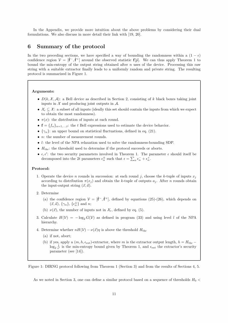
6 Summary of the protocolIn the two preceding sections, we have specified a way of bounding the randomness within a (1 − ε)confidence region V = [f−, f+] around the observed statistic f [p]. We can thus apply Theorem 1 tobound the min-entropy of the output string obtained after n uses of the device. Processing this rawstring with a suitable extractor finally leads to a uniformly random and private string. The resultingprotocol is summarized in Figure 1.

Arguments:

• D(k,X ,A): a Bell device as described in Section 2, consisting of k black boxes taking jointinputs in X and producing joint outputs in A.

• Xr ⊆ X : a subset of all inputs (ideally this set should contain the inputs from which we expectto obtain the most randomness).

• π(x): the distribution of inputs at each round.• f = fαα=1,...,t: the t Bell expressions used to estimate the device behavior.• γα: an upper bound on statistical fluctuations, defined in eq. (21).• n: the number of measurement rounds.• l: the level of the NPA relaxation used to solve the randomness-bounding SDP.• Hthr: the threshold used to determine if the protocol succeeds or aborts.• ε, ε′: the two security parameters involved in Theorem 1. The parameter ε should itself be

decomposed into the 2t parameters ε±α such that ε =∑α ε−α + ε+α .

Protocol:

1. Operate the device n rounds in succession: at each round j, choose the k-tuple of inputs xjaccording to distribution π(xj) and obtain the k-tuple of outputs aj . After n rounds obtainthe input-output string (~x,~a).

2. Determine(a) the confidence region V = [f−, f+], defined by equations (25)-(26), which depends on

(~x,~a), γα, ε±α and n;(b) ν(~x), the number of inputs not in Xr, defined by eq. (5).

3. Calculate H(V) = − log2G(V) as defined in program (33) and using level l of the NPAhierarchy.

4. Determine whether nH(V)− ν(~x)η is above the threshold Hthr

(a) if not, abort;(b) if yes, apply a (m,h, εext)-extractor, where m is the extractor output length, h = Hthr −

log21ε′ is the min-entropy bound given by Theorem 1, and εext the extractor’s security

parameter (see [14]).

Figure 1: DIRNG protocol following from Theorem 1 (Section 3) and from the results of Sections 4, 5.

As we noted in Section 3, one can define a similar protocol based on a sequence of thresholds H0 <

11

H1 < · · · < H` rather than a single one, introducing intermediate levels of success in the protocol. Oneadvantage of this is that we do not need to determine what threshold we expect the device to reachand risk failing the protocol with high probability if we overestimated Hthr. See Section III.D of [14] fordetails.

7 DiscussionWe have introduced a family of protocols, each characterized by a choice of t Bell expressions fα, arandomness-generating input set Xr, and an input distribution π(x). This family contains as a specialcase the protocols introduced in [3, 14, 15], which correspond to the case where a single Bell expressionf is used (t = 1) and where the randomness-bounding function covers all inputs (Xr = X ). The mainnovelty introduced in the present work is that we can take into account information from more Bellexpressions (t ≥ 1) and can tailor the randomness analysis to a subset of all possible inputs (Xr ⊆ X ).

In order to discuss these new aspects, in the following sections we illustrate our protocol on a concreteexample. The scenario in this example has two parties (k = 2), two measurement settings per party(X = 0, 12), and two outcome possibilities per measurement (A = 0, 12). We consider a devicebehavior

p = vpext + (1− v)u (34)

for v = 0.99, arising from a mixture of white noise u and the extremal quantum behavior pext that achievesmaximal violation of the Iβ1 tilted-CHSH inequality introduced in [21], with β = 2 cos(2θ)/

√1 + sin2(2θ)

for θ = π/8. The tilted-CHSH expression is defined as

Iβ1 = β〈A0〉+ 〈A0B0〉+ 〈A0B1〉+ 〈A1B0〉 − 〈A1B1〉 . (35)

The extremal behavior can be achieved by a pair of partially entangled qubits |φ〉 = cos θ |00〉+ sin θ |11〉measured with observables

A0 = σx , A1 = σz , (36a)B0 = cosµσz + sinµσx , B1 = cosµσz − sinµσx , (36b)

with tanµ = sin 2θ. (Note the difference in notation from [21]: we relabelled the inputs 1 and 2 to 0 and1, respectively.)

The resulting correlations have the property of giving more predictable outcomes for a subset ofmeasurement inputs. For θ = π/8, the two measurement settings that give more predictable outcomes,x = (0, 0) and x = (0, 1), have a guessing probability of about 0.775 in the ideal (v = 1) case where Iβ1 ismaximally violated. On the other hand, the two measurement settings with less predictable outcomes,x = (1, 0) and x = (1, 1), have guessing probabilities of about 0.496.

In the analysis of randomness, we will consider two choices for the randomness generating subset Xr:the full input set Xr = X and the more restricted choice Xr = (1, 0), which is one of the two settingsthat give less predictable measurements in pext.

Furthermore, we will estimate three different Bell expressions, all defined in terms of the followingcorrelators:

〈Ax1〉 =∑

a1,a2,x2∈0,1

(−1)a1π2(x2 | x1)p(a1a2 | x1x2) x1 ∈ 0, 1, (37a)

〈Bx2〉 =∑

a1,a2,x1∈0,1

(−1)a2π1(x1 | x2)p(a1a2 | x1x2) x2 ∈ 0, 1, (37b)

〈Ax1Bx2〉 =∑

a1,a2∈0,1

(−1)a1+a2p(a1a2 | x1x2) x1, x2 ∈ 0, 1. (37c)

The weights π1(x1 | x2) and π2(x2 | x1) represent the two conditional local input distributions definedwith respect to the joint input distribution π(x1x2).1

1Note that for a no-signaling behavior, we could equivalently use any arbitrary set of probability weights in placeof π1(x1 | x2) or π2(x2 | x1). We choose this specific set of weights because it provides a better estimator for the

12

The expressions we will evaluate are the CHSH expression

Ichsh = 〈A0B0〉+ 〈A0B1〉+ 〈A1B0〉 − 〈A1B1〉 , (38)

the tilted-CHSH expression Iβ1 (35) and the “optimal” expressions for the chosen device behavior (34):

Ip = 10.610− 1.859 〈A0〉 − 1.733 〈A1〉+ 0.499 〈B0〉 − 2.196 〈B1〉− 3.109 〈A0B0〉 − 2.945 〈A0B1〉 − 2.610 〈A1B0〉+ 4.343 〈A1B1〉

(39)

and

Iallp = 3.131 + 0.126 〈A0〉 − 0.428 (〈B0〉+ 〈B1〉)

− 0.673 (〈A0B0〉+ 〈A0B1〉)− 1.002 (〈A1B0〉 − 〈A1B1〉) .(40)

These last two Bell expressions are “optimal” Bell expressions in the following sense. As already observedin [19, 20], the dual of problem (32) (see eq. (51) in the Appendix), when applied to a device characterizedby its full behavior (i.e., fa,x[p] = p(a | x) so that f [p] = p), finds a Bell expression Ip such that theamount of randomness certified from Ip[p] with respect to the measurement setting x = (1, 0) is equalto the amount of randomness that can be certified from the entire table of probabilities p(a | x) (again,with respect to the measurement x = (1, 0)). Thus, to each device behavior p is associated a single Bellexpression Ip that is optimal for p from the point of view of randomness.2 Likewise, Iall

p is defined withrespect to all inputs x ∈ X rather than the subset (1, 0).

7.1 Bounding randomness for all inputs with one Bell expression (Xr = X ,t = 1)

Before discussing the novelties introduced in this work, let us start by briefly reviewing the case t = 1and Xr = X , which corresponds to the protocols introduced in [3, 14, 15]. In this case, ν(~x), thenumber of inputs not in Xr, is always equal to zero, and according to Theorem 1, the min-entropy of theoutput string is roughly equal to nH(V). Furthermore, the confidence region V reduces to a confidenceinterval [f−, f+] around the estimated Bell violation f . Usually, the values of f that we expect toobtain in the protocol will fall in a region where H(f) is either monotonically increasing or decreasingwith f , i.e., the interval is within either the upward- or downward-sloped region of the convex functionH(f). For instance, if f is the CHSH expression, we may assume that the devices have been designedso that with very high probability f ≥ 2. In that region, H(f) is indeed increasing with f (i.e., therandomness increases for increasing values of the CHSH expression). Let us assume for definiteness thatH is increasing (the same kind of reasoning can be done if H is decreasing). Since we are looking for theminimal value of H in the region V (see Lemma 2), it is then sufficient, as done in [3, 14, 15], to take aone-sided interval [f−,∞[, and the minimal value of H in the interval will then be H(f−). Consideringagain our CHSH example, we are interested in a guarantee that the CHSH value is above some threshold,which determines the randomness we can certify in the worst case, but it is useless to know that it isbounded from above (see also discussion at the end of Section 4). Taking the definition eq. (25) for f−,we thus get that the min-entropy of the output string is bounded (roughly speaking3, and up to the

marginal correlators 〈Ax1 〉 and 〈Bx2 〉 when applied to the observed frequencies p(a1a2 | x1x2). Indeed, it can be seenfrom the definition of a Bell estimator f [p] in eq. (19) that the marginal correlators reduce to a natural definition basedon locally available data resulting only from the respective party’s interaction with their part of the device, namely,〈Ax1 〉 =

∑a1

(−1)a1 #(a1, x1)/(nπ1(x1)), and similarly for 〈Bx2 〉.2More accurately, there exist infinitely many Bell expressions that are equivalent to Ip up to terms that vanish for no-

signaling behaviors. In order to pick one that tolerates the small signaling fluctuations present in our behavior estimatorp, we run the computation of Ip in the 8-dimensional space of correlators, rather than the overspecified 16-dimensionalparametrization of quantum behaviors in terms of the probabilities p(a1a2 | x1x2). We translate this expression back toa unique standard form (1) using definition (37) for the correlators. This ensures that the solution to the dual program(51) picked by our solver among many equivalent expressions does not contain terms that blow up under small signalingfluctuations. See also [26] for a finer analysis of noise tolerance in equivalent Bell expressions.

3Equation (41) and the similar approximate bounds that follow should be understood as informal statements givingan order of magnitude for the min-entropy lower bound. Contrary to the statement of Theorem 1, this informal bounddirectly involves the estimator f , which is a random variable. As such, it might be subject to improbable but extremefluctuations, in which case the bound does not correctly characterize the device. In comparison, the min-entropy bound ofTheorem 1 is expressed in terms of a fixed threshold. Furthermore, the Theorem also accounts for the unlikely event thata device reaches this threshold only by chance.

13

− log2(1/ε′) correction) as

Hmin & nH

(f − γ

√2n

ln 1ε

). (41)

This is precisely the result of [3, 14, 15], whose interpretation is quite intuitive: the min-entropy aftern runs is equal to n times the min-entropy for a single run, evaluated on the observed Bell violation foffset by a statistical parameter µ = γ

√(2/n) ln(1/ε). This correction accounts for the fact that even if

a device has been built such that it produces a target Bell violation, statistical fluctuations may pushthe observed violation above what is expected.

This statistical correction depends on the security parameter ε and decreases with the number ofruns n. It also depends on the prefactor γ defined in eq. (21). This prefactor depends on the choice ofBell expression f , and also importantly on the input distribution π(x).

As discussed in [3, 14], the input distribution can be suitably chosen to optimize the ratio Rout/Rinof the randomness that is produced to the randomness that is consumed when choosing the inputs. Theidea is that if at each run one selects with very high probability a given input x = x∗, then the resultingdistribution π(x) can be sampled from a small number of initial uniform bits Rin, which should improvethe ratio Rout/Rin. However, this will also lower Rout because observations involving the other inputsx 6= x∗ will be less frequent, which will reduce the statistical accuracy. Consider for instance, as in [3, 14],the case where the input x∗ is chosen with probability π(x∗) = 1−κn−δ for some constants κ and δ, andthe other inputs are chosen with probability π(x) = κ′n−δ, where κ′ = κ/(|X | − 1) for normalization.Then the initial randomness Rin required to choose the inputs according to this distribution will be ofsize O(n1−δ lnnδ) (i.e., roughly n times the Shannon entropy of the input distribution, see Theorem 2in [14]). On the other hand, according to eq. (41), the output randomness will be of size Ω(n) as long asthe statistical correction, of order γ/

√n, remains bounded by a constant. Since, according to eq. (21),

γ ' 1/(minx π(x)) we get that the statistical correction is of order γ/√n = O(nδ− 1

2 ) and thus that weshould take δ ≤ 1

2 . We can thus hope at best a quadratic expansion wherein O(n 12 lnn 1

2 ) initial bits areconsumed and Ω(n) are produced.

Note that the initial randomness for choosing the inputs only needs to be random with respect tothe devices, but can be publicly announced to the adversary without compromising the privacy of theoutput string [14, 27]. One can thus view the above protocols as producing private randomness frompublic randomness. From this perspective, the “expansion” efficiency of the protocol is less relevantsince the final and initial randomness correspond to different resources that do not necessarily have tobe compared on the same footing.

We generated random samples of n input-output pairs ~a, ~x from the behavior p corresponding toequation (34) with the following input distribution

π(x) =

1− 32n−1/5 if x = (1, 0) ,

12n−1/5 otherwise.

(42)

Note that as n grows, the input distribution becomes strongly biased to select x = (1, 0) most of thetime.

We performed this sampling independently for different values of n between 100 and 3 × 1018. Foreach value of n, we repeated this sampling 300 times in order to show the variation of our result overseveral simulations.

The corresponding min-entropy rate bound (that is, (41) divided by n) for ε = 10−6 is represented inFigure 2 as a function of the number of runs n for different Bell expressions. The curves in this plot andthe ones that follow (Figures 2–5) show the values for the first simulation out of the 300, and the rangeof values taken over all 300 simulations is drawn as a shaded area behind each curve. In some instances,usually for high values of n, the area is invisible, which indicates a negligible variation across simulationruns. All curves are obtained by solving the program (33) in its dual form (56) (see Appendix) at level 2of the NPA hierarchy. All optimizations were performed using the Matlab toolboxes Yalmip [28] andSeDuMi [29].

As we can see, the expression Iβ1 gives the worst results. The reason for this is that the inequality issuited to the extremal behavior pext rather than the imperfect behavior we simulated (i.e., in equation(34), the case of perfect visibility v = 1 rather than v = 0.99). On the other hand, the expression

14

102 104 106 108 1010 1012 1014 1016 1018

0

0.2

0.4

0.6

n

Hm

in/n

Iallp estimator, Xr = X

Ichsh estimator, Xr = XIβ1 estimator, Xr = X

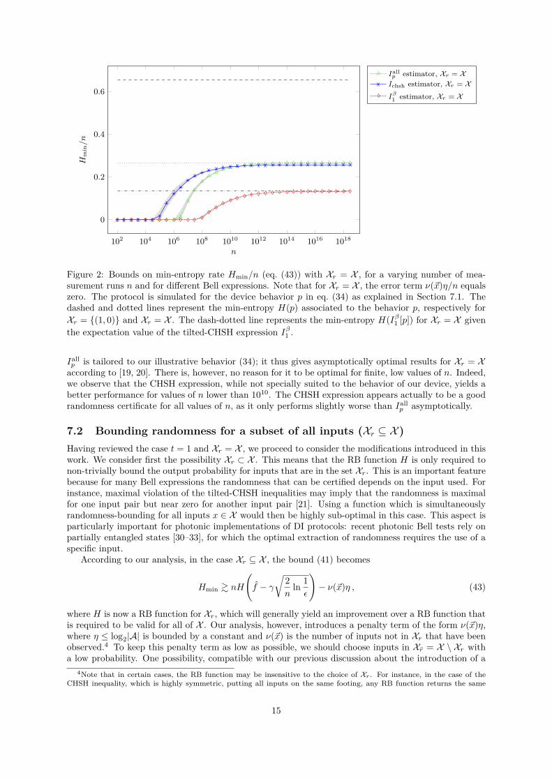
Figure 2: Bounds on min-entropy rate Hmin/n (eq. (43)) with Xr = X , for a varying number of mea-surement runs n and for different Bell expressions. Note that for Xr = X , the error term ν(~x)η/n equalszero. The protocol is simulated for the device behavior p in eq. (34) as explained in Section 7.1. Thedashed and dotted lines represent the min-entropy H(p) associated to the behavior p, respectively forXr = (1, 0) and Xr = X . The dash-dotted line represents the min-entropy H(Iβ1 [p]) for Xr = X giventhe expectation value of the tilted-CHSH expression Iβ1 .

Iallp is tailored to our illustrative behavior (34); it thus gives asymptotically optimal results for Xr = Xaccording to [19, 20]. There is, however, no reason for it to be optimal for finite, low values of n. Indeed,we observe that the CHSH expression, while not specially suited to the behavior of our device, yields abetter performance for values of n lower than 1010. The CHSH expression appears actually to be a goodrandomness certificate for all values of n, as it only performs slightly worse than Iall

p asymptotically.

7.2 Bounding randomness for a subset of all inputs (Xr ⊆ X )Having reviewed the case t = 1 and Xr = X , we proceed to consider the modifications introduced in thiswork. We consider first the possibility Xr ⊂ X . This means that the RB function H is only required tonon-trivially bound the output probability for inputs that are in the set Xr. This is an important featurebecause for many Bell expressions the randomness that can be certified depends on the input used. Forinstance, maximal violation of the tilted-CHSH inequalities may imply that the randomness is maximalfor one input pair but near zero for another input pair [21]. Using a function which is simultaneouslyrandomness-bounding for all inputs x ∈ X would then be highly sub-optimal in this case. This aspect isparticularly important for photonic implementations of DI protocols: recent photonic Bell tests rely onpartially entangled states [30–33], for which the optimal extraction of randomness requires the use of aspecific input.

According to our analysis, in the case Xr ⊆ X , the bound (41) becomes

Hmin & nH

(f − γ

√2n

ln 1ε

)− ν(~x)η , (43)

where H is now a RB function for Xr, which will generally yield an improvement over a RB function thatis required to be valid for all of X . Our analysis, however, introduces a penalty term of the form ν(~x)η,where η ≤ log2|A| is bounded by a constant and ν(~x) is the number of inputs not in Xr that have beenobserved.4 To keep this penalty term as low as possible, we should choose inputs in Xr = X \ Xr witha low probability. One possibility, compatible with our previous discussion about the introduction of a

4Note that in certain cases, the RB function may be insensitive to the choice of Xr. For instance, in the case of theCHSH inequality, which is highly symmetric, putting all inputs on the same footing, any RB function returns the same

15

102 104 106 108 1010 1012 1014 1016 1018

0

0.5

1

1.5(ν

(~x)/n

)η

102 104 106 108 1010 1012 1014 1016 1018

0

0.2

0.4

0.6

n

Hm

in/n

Ip estimator, Xr = (1, 0)Iβ1 estimator, Xr = (1, 0)Iallp estimator, Xr = X

Ichsh estimator, Xr = XIβ1 estimator, Xr = X

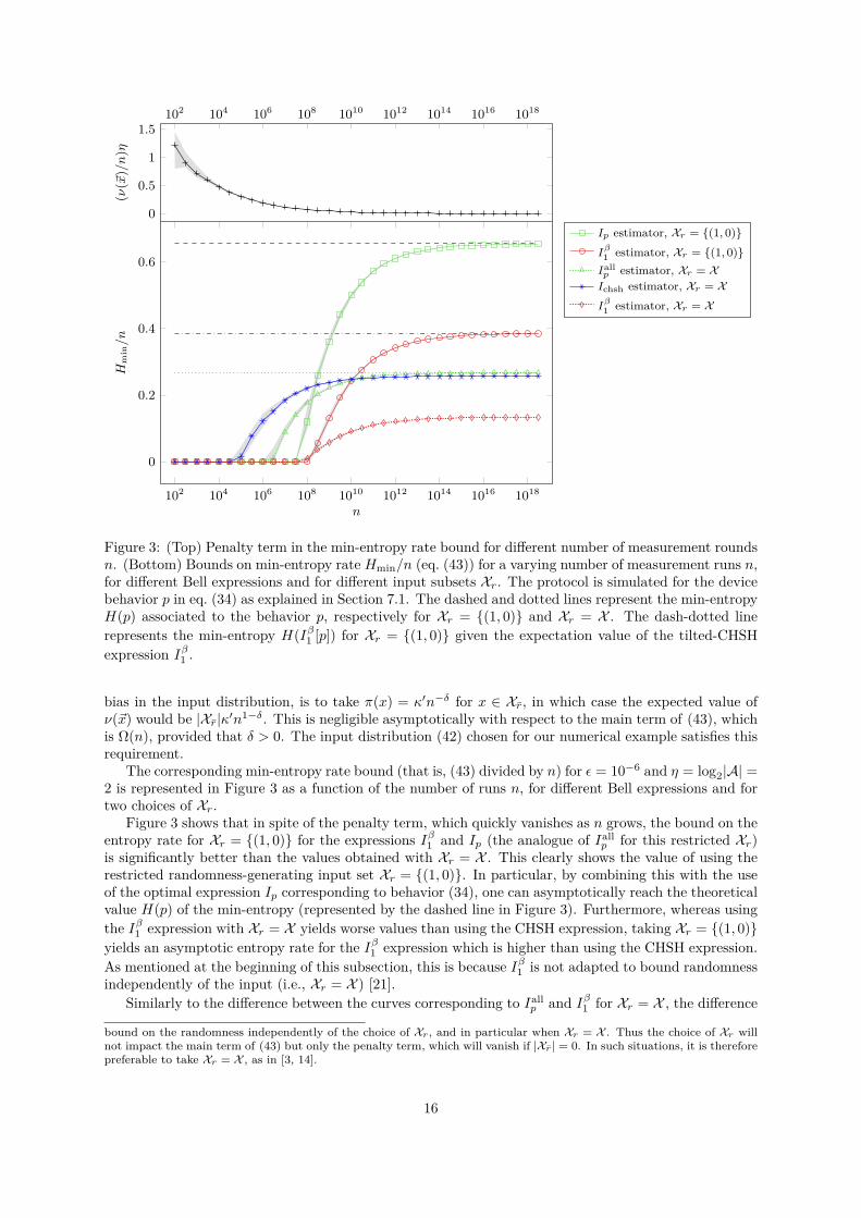
Figure 3: (Top) Penalty term in the min-entropy rate bound for different number of measurement roundsn. (Bottom) Bounds on min-entropy rate Hmin/n (eq. (43)) for a varying number of measurement runs n,for different Bell expressions and for different input subsets Xr. The protocol is simulated for the devicebehavior p in eq. (34) as explained in Section 7.1. The dashed and dotted lines represent the min-entropyH(p) associated to the behavior p, respectively for Xr = (1, 0) and Xr = X . The dash-dotted linerepresents the min-entropy H(Iβ1 [p]) for Xr = (1, 0) given the expectation value of the tilted-CHSHexpression Iβ1 .

bias in the input distribution, is to take π(x) = κ′n−δ for x ∈ Xr, in which case the expected value ofν(~x) would be |Xr|κ′n1−δ. This is negligible asymptotically with respect to the main term of (43), whichis Ω(n), provided that δ > 0. The input distribution (42) chosen for our numerical example satisfies thisrequirement.

The corresponding min-entropy rate bound (that is, (43) divided by n) for ε = 10−6 and η = log2|A| =2 is represented in Figure 3 as a function of the number of runs n, for different Bell expressions and fortwo choices of Xr.

Figure 3 shows that in spite of the penalty term, which quickly vanishes as n grows, the bound on theentropy rate for Xr = (1, 0) for the expressions Iβ1 and Ip (the analogue of Iall

p for this restricted Xr)is significantly better than the values obtained with Xr = X . This clearly shows the value of using therestricted randomness-generating input set Xr = (1, 0). In particular, by combining this with the useof the optimal expression Ip corresponding to behavior (34), one can asymptotically reach the theoreticalvalue H(p) of the min-entropy (represented by the dashed line in Figure 3). Furthermore, whereas usingthe Iβ1 expression with Xr = X yields worse values than using the CHSH expression, taking Xr = (1, 0)yields an asymptotic entropy rate for the Iβ1 expression which is higher than using the CHSH expression.As mentioned at the beginning of this subsection, this is because Iβ1 is not adapted to bound randomnessindependently of the input (i.e., Xr = X ) [21].

Similarly to the difference between the curves corresponding to Iallp and Iβ1 for Xr = X , the difference

bound on the randomness independently of the choice of Xr, and in particular when Xr = X . Thus the choice of Xr willnot impact the main term of (43) but only the penalty term, which will vanish if |Xr| = 0. In such situations, it is thereforepreferable to take Xr = X , as in [3, 14].

16

between the asymptotic entropy rates reached by using the expressions Ip and Iβ1 for Xr = (1, 0) iscaused by the imperfect visibility parameter v = 0.99 in the simulated behavior (34).

Making the right choice of Bell expression and input subset Xr depends not only on the device, butalso on the value of n. Indeed, while Ip is an optimal expression for certifying randomness in this specificdevice with respect to the input subset Xr = (1, 0), this is only the case asymptotically. For small n,Figure 3 suggests that the CHSH expression has a better resistance to statistical fluctuations than theother expressions we considered, regardless of Xr.

Note that we did not attempt to optimize the choice of input distribution and it is possible that adifferent choice of π(x) would lead to better bounds in Figure 3 for the two curves with Xr = (1, 0).

7.3 Bounding randomness from several Bell expressions (t ≥ 1)As we have seen, the right choice of a single Bell expression in the analysis of randomness is not straight-forward, except for large values of n where Ip becomes optimal. In this regime, it would seem perfectlyadmissible to perform tests on the device before running the actual randomness generation protocol,in order to estimate p and use this information to find an “optimal” Bell expression Ip′ as describedabove, which can afterwards be used in the randomness generation protocol proper. However, there aredisadvantages to this method.

Firstly, to find an expression Ip′ that performs comparably to the optimal Ip for the device behaviorp, we must know p to a sufficiently high accuracy. In a black box scenario where imperfections cannot beruled out, this means that a significant number of measurements must be performed in order to evaluatethe behavior to great precision. Since the Bell expression needs to be fixed in advance of the protocol,those evaluation rounds cannot be taken from measurement rounds of the protocol and must instead bethrown away. In addition, the behavior of the devices may vary in time, unlike our i.i.d. choice (34), dueto drifts in the experimental set-up for example. In that case, one would need to periodically estimatep and rederive the corresponding optimal Bell expression on some subset of the measurement data thatneeds to be thrown away. Finding an expression Ip′ also requires methods of inference of the behaviorof the device from a finite sample: indeed, the estimated behavior (18) cannot be used directly to find acandidate Ip, as p almost always violates the no-signaling conditions. There exist different approachesto this inference (see for instance [20, 34–37]), so a nontrivial choice must be made.

Finally, even ignoring the problem of estimating the unknown behavior p, the associated data loss, orthe drift of p over time, we saw in the previous section and in Figure 3 that the choice of a Bell expressionis not straightforward when considering different values of n. For example, the asymptotically optimalexpression Ip as formulated in [19, 20] is generally not the best for low values of n. There is thus nogeneral method to guide the choice of a Bell expression for a given n.

In order to avoid the above problems associated to the use of a single Bell expression,5 we now turnto the second element introduced in this work: the possibility to estimate the randomness from t > 1Bell expressions, and in particular from the full set of observed frequencies of occurrence p = p(a | x)as defined in eq. (18).

When we have more than one Bell expression, the bound (43) generalizes to

Hmin & nH(

[f−, f+])− ν(~x)η , (44)

where the one-dimensional interval [f−,∞] has simply been replaced with the multidimensional region[f−, f+]. As before the limits of the region depend on the security parameter ε, the constants γα, andthey become smaller with the number of runs n (see equations (25) and (26)).

Increasing the number of Bell expressions can have both beneficial and detrimental consequences.We can reach an understanding of this by considering the optimization problem (33) that definesH([f−, f+]) = − log2G([f−, f+]). This problem essentially evaluates the randomness of a certain quan-tum behavior p such that f− ≤ f [p] ≤ f+. Each vector component of this constraint defines two affine

5Note that another issue is the choice of a randomness-generating input set Xr. The set Xr maximizing the randomnessgeneration rate depends obviously on the underlying behavior p, but also on the number of rounds n, as illustrated inFig. 3. In practice, setting Xr could be the result of an informed choice based on prior information about the behavior ofthe devices or a rough estimate of it made before running the protocol. It is reasonable to expect, as we do in our numericalsimulation, that the optimal set Xr is only weakly sensitive to fluctuations or drifts of the experimental set-up, since ittakes its value from a discrete set. The use of a fixed set Xr is thus less problematic than the use of a fixed Bell estimator.

17

102 104 106 108 1010 1012 1014 1016 1018

0

0.2

0.4

0.6

n

Hm

in/n

4 CHSH permutations+ 4 local correlators,Xr = (1, 0)4 CHSH permutations+ 4 local correlators,Xr = XIp estimator, Xr = (1, 0)Ichsh estimator, Xr = X

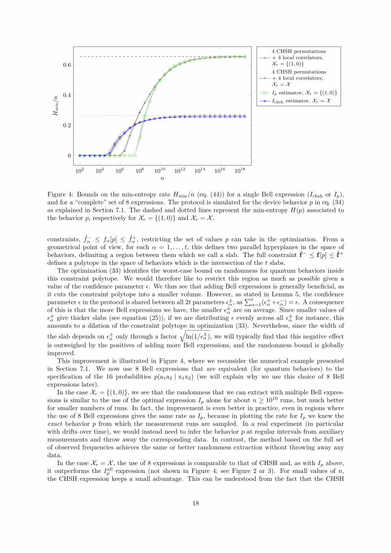
Figure 4: Bounds on the min-entropy rate Hmin/n (eq. (44)) for a single Bell expression (Ichsh or Ip),and for a “complete” set of 8 expressions. The protocol is simulated for the device behavior p in eq. (34)as explained in Section 7.1. The dashed and dotted lines represent the min-entropy H(p) associated tothe behavior p, respectively for Xr = (1, 0) and Xr = X .

constraints, f−α ≤ fα[p] ≤ f+α , restricting the set of values p can take in the optimization. From a

geometrical point of view, for each α = 1, . . . , t, this defines two parallel hyperplanes in the space ofbehaviors, delimiting a region between them which we call a slab. The full constraint f− ≤ f [p] ≤ f+

defines a polytope in the space of behaviors which is the intersection of the t slabs.The optimization (33) identifies the worst-case bound on randomness for quantum behaviors inside

this constraint polytope. We would therefore like to restrict this region as much as possible given avalue of the confidence parameter ε. We thus see that adding Bell expressions is generally beneficial, asit cuts the constraint polytope into a smaller volume. However, as stated in Lemma 5, the confidenceparameter ε in the protocol is shared between all 2t parameters ε±α , as

∑tα=1(ε+α +ε−α ) = ε. A consequence

of this is that the more Bell expressions we have, the smaller ε±α are on average. Since smaller values ofε±α give thicker slabs (see equation (25)), if we are distributing ε evenly across all ε±α for instance, thisamounts to a dilation of the constraint polytope in optimization (33). Nevertheless, since the width ofthe slab depends on ε±α only through a factor

√ln(1/ε±α ), we will typically find that this negative effect

is outweighed by the positives of adding more Bell expressions, and the randomness bound is globallyimproved.

This improvement is illustrated in Figure 4, where we reconsider the numerical example presentedin Section 7.1. We now use 8 Bell expressions that are equivalent (for quantum behaviors) to thespecification of the 16 probabilities p(a1a2 | x1x2) (we will explain why we use this choice of 8 Bellexpressions later).

In the case Xr = (1, 0), we see that the randomness that we can extract with multiple Bell expres-sions is similar to the use of the optimal expression Ip alone for about n ≥ 1010 runs, but much betterfor smaller numbers of runs. In fact, the improvement is even better in practice, even in regions wherethe use of 8 Bell expressions gives the same rate as Ip, because in plotting the rate for Ip we knew theexact behavior p from which the measurement runs are sampled. In a real experiment (in particularwith drifts over time), we would instead need to infer the behavior p at regular intervals from auxiliarymeasurements and throw away the corresponding data. In contrast, the method based on the full setof observed frequencies achieves the same or better randomness extraction without throwing away anydata.

In the case Xr = X , the use of 8 expressions is comparable to that of CHSH and, as with Ip above,it outperforms the Iall

p expression (not shown in Figure 4; see Figure 2 or 3). For small values of n,the CHSH expression keeps a small advantage. This can be understood from the fact that the CHSH

18

expression itself is part of the set of 8 expressions that we used in Figure 4. The difference betweenthe two curves therefore results from a trade-off between a better estimation of randomnes from moreexpressions and the negative effect of wider margins ε±α in the confidence region.

In the remainder of this section, we discuss in more detail how to choose a good set of Bell expressionsfor the protocol. For this, let us start by considering our protocol when n→∞. In this asymptotic limit,the interval [f−, f+] narrows down towards the point f = f [p(a | x)], which is just the value of the t Bellexpressions f computed on the experimentally observed frequencies p(a |x). If the bias towards inputs inXr is appropriately chosen (as discussed previously), then the relative contribution of the penalty termvanishes as n→∞ and the bound (44) becomes in the asymptotic limit, up to sublinear terms,

Hmin & nH(f) . (45)

Furthermore, in the case where the device behaves in an i.i.d. way according to a behavior p, then,asymptotically, f → f [p]. If one chooses enough Bell expressions as to fully characterize the behavior ofthe devices (for instance, by using an estimator for each probability p(a | x)), f thus becomes equivalentto the knowledge of p and the above bound converges to the maximal min-entropy bound one can obtainfrom p given Xr, as characterized in [19, 20]. In this sense, and as seen in Figure 4, our protocol isasymptotically optimal.

Note that there are different sets of Bell estimators that are asymptotically equivalent to the knowl-edge of the full set of probabilities p(a | x). For instance in a bipartite Bell experiment with two inputsand two outputs there are 16 probabilities p(a | x) = p(a1a2 | x1x2) with a1, a2, x1, x2 ∈ 0, 1 and thus16 associated Bell expressions e1, . . . , e16 defined by eα[p] = p(a1a2 | x1x2), with one value of α for eachof the possible values of (a1, a2, x1, x2). But since the probabilities p(a | x) satisfy normalization and no-signaling, they are uniquely specified by the 8 correlators of eq. (37), which constitute 8 Bell expressionsg1, . . . , g8, where g1 and g2 are the first party’s two marginal correlators 〈Ax1〉, g3 and g4 are the secondparty’s 〈Bx2〉, and g4, . . . , g8 are the four bipartite correlators 〈Ax1Bx2〉.

Alternatively, the probabilities are also equivalent to the 8 expressions h1, . . . , h8 with hα = gα forα = 1, . . . , 4, and hα for α = 5, . . . , 8 are four linearly independent permutations of the CHSH expression,generalizing (38):

Iy1,y2chsh =

∑x1,x2∈0,1

(−1)(x1+y1)(x2+y2)〈Ax1Bx2〉 y1, y2 ∈ 0, 1. (46)

As we increase the number of rounds, all these possible choices become equivalent, since the intervals[e−, e+], [g−, g+], [h−, h+] define constraint polytopes in the space of behaviors p that asymptoticallyintersect the quantum set at the same unique point. However, the choice of one set of estimators overanother could make a difference for finite n.

Generally speaking, when choosing which Bell expressions to use for a fixed number t, we may preferthat as many of them as possible be linearly independent. Consider t − 1 Bell expressions and theirassociated slabs, which define a constraint polytope. In the absence of any meaningful informationconcerning the behavior of the objective function of (33) within its feasible set, the choice of a t-thBell expression should be dictated by the resulting reduction of the constraint polytope: cutting a largevolume out is more likely to reduce the maximum of (33). As n grows large and the slabs grow thinner,the best way to reduce this volume is to choose a Bell expression that is linearly independent from thet− 1 previous ones, if possible. We can easily understand this in the asymptotic limit: as we mentionedabove, the optimization converges to H(f), and with enough linearly independent Bell expressions, f [p]uniquely defines p, hence H(f) = H(p). At this point, adding more expressions only makes f [p] a moreredundant definition of p, which does not improve the randomness bound. On the other hand, with toofew independent Bell expressions, f = f [p] is compatible with many values of p, and the worst value iswhat ends up determining H(f).

In addition, we see that there is no need for Bell expressions that are purely signaling, i.e., that havea constant value for all no-signaling behaviors p. Indeed, since the feasible region of (33) is defined bythe intersection of the slabs and the quantum set, constraints deriving from purely signaling expressionsare trivial in this region, and therefore do not contribute to improve the randomness bound.

Combining these two conclusions also indicates that we should avoid Bell expressions that are onlylinearly dependent up to purely signaling terms. This implies for instance that the sets g1, . . . , g8 orh1, . . . , h8 should be preferred over e1, . . . , e16. This is indeed what we find, as illustrated in Figure 5.

19

102 104 106 108 1010 1012 1014 1016 1018

0

0.2

0.4

0.6

n

Hm

in/n

4 CHSH permutations+ 4 local correlators, h8 correlators, gEstimated probabilities, e

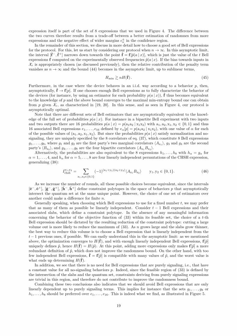
Figure 5: Bounds on the min-entropy rateHmin/n (eq. (44)) with Xr = (1, 0) for three (asymptotically)equivalent sets of Bell expressions. The protocol is simulated for the device behavior p in eq. (34) asexplained in Section 7.1. The dashed line represents the min-entropy H(p) associated to the behavior pfor Xr = (1, 0).

Note that the sets g1, . . . , g8 and h1, . . . , h8 only differ by a linear transformation, but the second setyields better results for the same (finite) number of rounds n. With respect to optimization (33), thismeans that the feasible set for h1, . . . , h8 excluded the optimum obtained for g1, . . . , g8. This might berelated to the fact that in this scenario of two parties with two inputs and two outputs, the four versionsof the CHSH inequalities constitute the facets that separate local from nonlocal behaviors, and theymight therefore serve as better measures of nonlocality and randomness than the correlators 〈Ax1Bx2〉.

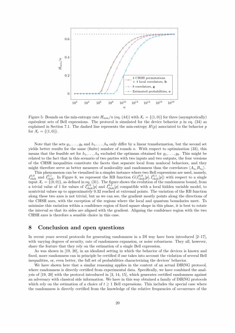
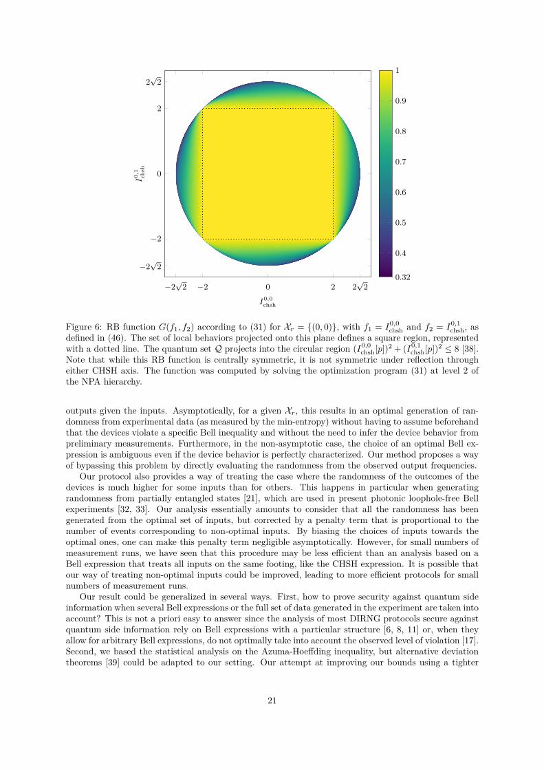
This phenomenon can be visualized in a simpler instance where two Bell expressions are used, namely,I0,0chsh and I0,1

chsh. In Figure 6, we represent the RB function G(I0,0chsh[p], I0,1

chsh[p]) with respect to a singleinput Xr = (0, 0), as defined in eq. (31). The figure shows the evolution of the randomness bound, froma trivial value of 1 for values of I0,0

chsh[p] and I0,1chsh[p] compatible with a local hidden variable model, to

nontrivial values up to approximately 0.32 reached at extremal points. The variation of the RB functionalong these two axes is not trivial, but as we can see, the gradient mostly points along the directions ofthe CHSH axes, with the exception of the regions where the local and quantum boundaries meet. Tominimize this variation within a confidence region of fixed square shape in this plane, it is best to rotatethe interval so that its sides are aligned with the gradient. Aligning the confidence region with the twoCHSH axes is therefore a sensible choice in this case.

8 Conclusion and open questionsIn recent years several protocols for generating randomness in a DI way have been introduced [2–17],with varying degrees of security, rate of randomness expansion, or noise robustness. They all, however,share the feature that they rely on the estimation of a single Bell expression.

As was shown in [19, 20], in an idealized setting in which the behavior of the devices is known andfixed, more randomness can in principle be certified if one takes into account the violation of several Bellinequalities, or, even better, the full set of probabilities characterizing the devices’ behavior.

We have shown here that a similar reasoning applies in the context of an actual DIRNG protocol,where randomness is directly certified from experimental data. Specifically, we have combined the anal-ysis of [19, 20] with the protocol introduced in [3, 14, 15], which generates certified randomness againstan adversary with classical side information. We have in this way obtained a family of DIRNG protocolswhich rely on the estimation of a choice of t ≥ 1 Bell expressions. This includes the special case wherethe randomness is directly certified from the knowledge of the relative frequencies of occurrence of the

20

−2√

2 −2 0 2 2√

2

−2√

2

−2

0

2

2√

2

I0,0chsh

I0,

1ch

sh

0.4

0.5

0.6

0.7

0.8

0.9

1

0.32

Figure 6: RB function G(f1, f2) according to (31) for Xr = (0, 0), with f1 = I0,0chsh and f2 = I0,1

chsh, asdefined in (46). The set of local behaviors projected onto this plane defines a square region, representedwith a dotted line. The quantum set Q projects into the circular region (I0,0

chsh[p])2 + (I0,1chsh[p])2 ≤ 8 [38].

Note that while this RB function is centrally symmetric, it is not symmetric under reflection througheither CHSH axis. The function was computed by solving the optimization program (31) at level 2 ofthe NPA hierarchy.

outputs given the inputs. Asymptotically, for a given Xr, this results in an optimal generation of ran-domness from experimental data (as measured by the min-entropy) without having to assume beforehandthat the devices violate a specific Bell inequality and without the need to infer the device behavior frompreliminary measurements. Furthermore, in the non-asymptotic case, the choice of an optimal Bell ex-pression is ambiguous even if the device behavior is perfectly characterized. Our method proposes a wayof bypassing this problem by directly evaluating the randomness from the observed output frequencies.

Our protocol also provides a way of treating the case where the randomness of the outcomes of thedevices is much higher for some inputs than for others. This happens in particular when generatingrandomness from partially entangled states [21], which are used in present photonic loophole-free Bellexperiments [32, 33]. Our analysis essentially amounts to consider that all the randomness has beengenerated from the optimal set of inputs, but corrected by a penalty term that is proportional to thenumber of events corresponding to non-optimal inputs. By biasing the choices of inputs towards theoptimal ones, one can make this penalty term negligible asymptotically. However, for small numbers ofmeasurement runs, we have seen that this procedure may be less efficient than an analysis based on aBell expression that treats all inputs on the same footing, like the CHSH expression. It is possible thatour way of treating non-optimal inputs could be improved, leading to more efficient protocols for smallnumbers of measurement runs.

Our result could be generalized in several ways. First, how to prove security against quantum sideinformation when several Bell expressions or the full set of data generated in the experiment are taken intoaccount? This is not a priori easy to answer since the analysis of most DIRNG protocols secure againstquantum side information rely on Bell expressions with a particular structure [6, 8, 11] or, when theyallow for arbitrary Bell expressions, do not optimally take into account the observed level of violation [17].Second, we based the statistical analysis on the Azuma-Hoeffding inequality, but alternative deviationtheorems [39] could be adapted to our setting. Our attempt at improving our bounds using a tighter

21

concentration inequality from Hoeffding [40] (called McDiarmid’s inequality in [39] after [41]) producedno visible difference in the plots. Another alternative, Bentkus’ inequality [39, 42], involves discretesummations with around n terms, which would grow too large in our simulations to be used as-is.Finally, we note that since DIRNG is not the only task where information from several Bell estimatorscan be exploited, a similar approach could be developed for other DI problems, such as DI quantum keydistribution.

AcknowledgmentsWe would like to thank the anonymous referees for the time dedicated to reviewing our manuscript andfor their useful comments.

We acknowledge financial support from the Fondation Wiener-Anspach, the Interuniversity Attrac-tion Poles program of the Belgian Science Policy Office under the grant IAP P7-35 photonics@be, andthe Fonds de la Recherche Scientifique F.R.S.-FNRS (Belgium). O. N.S. acknowledges financial sup-port through a grant of the Fonds pour la Formation à la Recherche dans l’Industrie et l’Agriculture(F.R.I.A.). C. B. acknowledges funding from the F.R.S.-FNRS through a Research Fellowship. J. S.was a postdoctoral researcher of the F.R.S.-FNRS at the time this research was carried out. S. P. is aResearch Associate of the F.R.S.-FNRS. All plots were produced using TikZ [43] and pgfplots [44].The heat map of Figure 6 was produced using Matplotlib [45].

A AppendixThe problems introduced in Section 5 are typical instances of conic programming. A conic program isan optimization problem of the form

maximizexi

k∑i=1〈ci, xi〉

subject tok∑i=1

Aixi = b

xi ∈ Ki i = 1, . . . , k ,

(47)

where b ∈ Rm, xi, ci ∈ Rni , Ai ∈ Rm×ni , and Ki are closed convex cones (i = 1, . . . , k). Here 〈c, x〉denotes the usual scalar product 〈c, x〉 =

∑nj=1 cjxj between vectors in Rn and a set K is a convex cone

if q1p1 + q2p2 belongs to K for any nonnegative scalars q1, q2 ≥ 0 and any p1, p2 in K.In other words, an optimization problem is a conic program if it involves the maximization of a linear

function of the optimization variables given linear constraints on such variables and the condition thatthey belong to a certain family of cones. Many familiar convex optimization problems, including linearand semidefinite programming, are instances of conic programming.

The problems (32) and (33), and their NPA relaxations, are also conic programs. Indeed, the set ofunnormalized behaviors Q and all of its NPA relaxations are clearly cones and all other constraints in(32) and (33) are linear in the variables pa,x. As we said earlier, the NPA relaxations of these problemsactually correspond to a specific type of conic programs, i.e., semidefinite programs.

Any conic program in the primal form (47) admits a dual formulation given by [46]

minimizey

〈b, y〉

subject to ATi y − ci ∈ K∗i i = 1, . . . , k(48)

where y ∈ Rm and K∗i = zi ∈ Rni : 〈zi, xi〉 ≥ 0, ∀xi ∈ Ki is the dual cone of Ki. Let α denote thevalue of the primal program (47) and β the value of the dual program (48). Then the strong dualitytheorem of conic programming says that if the primal program is feasible, has finite value α, and haspoints xi ∈ int(Ki) such that

∑ki=1Aixi = b, then the dual program is feasible and has finite value β = α

[46].

22

Let us determine the dual of the optimization problem (32). From now on, we take generically Qto denote the cone of unnormalized quantum behaviors or any of its NPA relaxations, as the analysis isidentical in both cases.

Let us first rewrite (32) in a form similar to (47). For this, define cax ∈ R|A|×|X| as the vector withcomponents cax(a′, x′) = δaa′δxx′ . Thus 〈cax, p〉 = p(a | x). Let b = (1, f1[p], . . . , ft[p]) ∈ R1+t. Let u beany Bell expression such that u[p] = Tr[p] for all no-signaling behaviors p, for instance u(a, x) = δx,x0

for some input x0 ∈ X . Let Aax be matrices in R1+t,|A|×|X| with components [Aax]1,a′x′ = u(a′, x′) and[Aax]1+α,a′x′ = fα(a′, x′) for α = 1, . . . , t. Then

G(f [p]) = maxpa,xa∈A,x∈Xr

∑a∈A,x∈Xr

〈cax, pa,x〉

subject to∑

a∈A,x∈Xr

Aaxpa,x = b

pa,x ∈ Q ∀a ∈ A,∀x ∈ Xr.

(49)

The dual is then readily given as

G(f [p]) = miny∈R1+t

〈b, y〉

subject to ATaxy − cax ∈ Q∗ ∀a ∈ A,∀x ∈ Xr ,(50)

where Q∗ is the dual cone of Q, that is, the set Q∗ = c ∈ R|A|×|X| : 〈c, p〉 ≥ 0, ∀p ∈ Q. Note thatthis dual cone can be identified with the set of Tsirelson inequalities for normalized behaviors, that is,the set Q∗ = (d0, d) ∈ R1+|A|×|X| : 〈d, p〉 ≤ d0, ∀p ∈ Q. Indeed, note that by normalization 〈u, p〉 = 1and thus an inequality 〈d, p〉 ≤ d0 valid for p ∈ Q can always be rewritten in the form 〈(d0u− d), p〉 ≥ 0,hence in the form 〈c, p〉 ≥ 0 for some suitable c. But an inequality 〈c, p〉 ≥ 0 is clearly valid for Q if andonly if it is valid for Q.

Using the explicit form of b, Aax, and cax and the above interpretation of Q∗, we can rewrite thedual (50) as

G(f [p]) = miny∈R1+t

y0 +t∑

α=1yαfα[p]

subject to p′(a | x) ≤ y0 +t∑

α=1yαfα[p′] ∀a ∈ A, ∀x ∈ Xr, ∀p′ ∈ Q.

(51)

The interpretation of this dual problem is immediate. We are seeking an affine function y0 +∑a yαfα[p]

satisfying the condition 1 in Definition 1—this is the constraint line of the optimization problem (51).Since the function is affine, it is also concave and the condition 2 in Definition 1 is also trivially satisfied.We are then searching for the best function of this form, i.e., the one that gives the lowest possible value(i.e., the most randomness) for the given Bell expectations f [p]. Note that considering an affine functionis actually not a restriction because the optimal function G(f [p]) is concave, and therefore it is equivalentto the envelope of its tangents, which are affine functions of f [p].

From the point of view of implementations, the condition that p′(a | x) ≤ y0 +∑α yαfα[p′] is valid

for Q can be cast as a search for a sum-of-squares decomposition of this inequality. When Q is one ofthe NPA relaxations of the quantum set, this is equivalent to solving a certain SDP, which turns out tobe, as expected, the dual of the original NPA problem.

23

Let us now determine the dual of the noisy problem (33), which we can rewrite as

G([f−, f+]) = maxpa,xa∈A,x∈Xr

τ ,κ∈Rt

∑a∈A,x∈Xr

pa,x(a | x)

subject to∑

a∈A,x∈Xr

Tr[pa,x] = 1

∑a∈A,x∈Xr

f [pa,x] + τ = f+

∑a∈A,x∈Xr

f [pa,x]− κ = f−

pa,x ∈ Q ∀a ∈ A, ∀x ∈ Xrτ ,κ ∈ Rt+ .

(52)

Again, let us rewrite in a form similar to (47). For this, define b ∈ R1+2t = (1, f+1 , . . . , f

+t , f

−1 , . . . , f

−t ).

Let Aax be matrices in R1+2t,|A|×|X| with components [Aax]1,a′x′ = u(a′, x′) and [Aax]1+α,a′x′ = fα(a′, x′)as above, and [Aax]1+t+α,a′x′ = fα(a′, x′), for α = 1, . . . , t. Additionally, we define two matrices A1, A2in R1+2t,t through [A1]1,α = 0, [A1]1+α,α′ = δα,α′ , [A1]1+t+α,α′ = 0 and [A2]1,α = 0, [A2]1+α,α′ = 0,[A2]1+t+α,α′ = −δα,α′ for α, α′ ∈ 1, . . . , t. Then

G([f−, f+]) = maxpa,xa∈A,x∈Xr

τ ,κ∈Rt

∑a∈A,x∈Xr

〈cax, pa,x〉

subject to∑

a∈A,x∈Xr

Aaxpa,x +A1τ +A2κ = b

pa,x ∈ Q ∀a ∈ A, ∀x ∈ Xrτ ,κ ∈ Rt+ .

(53)

The dual is then readily given as

G([f−, f+]) = minv∈R1+2t

〈b, v〉

subject to ATaxv − cax ∈ Q∗ ∀a ∈ A, ∀x ∈ XrAT1 v,A

T2 v ∈ Rt+

(54)

or, writing v = (v0, v1, . . . , vt, v′1, . . . , v

′t)

G([f−, f+]) = minv∈R1+2t

v0 +t∑

α=1vαf

+α +

t∑α=1

v′αf−α

subject to v0u+t∑

α=1(vα + v′α)fα − cax ∈ Q∗ ∀a ∈ A, ∀x ∈ Xr

vα ≥ 0, v′α ≤ 0 ∀α = 1, . . . , t .

(55)

Defining (y0, y+α , y

−α ) = (v0, vα,−v′α) and yα = vα + v′α = y+

α − y−α , we can reformulate this as

G([f−, f+]) = min(y0,y+,y−)∈R1+2t

y0 +t∑

α=1y+α f

+α −

t∑α=1

y−α f−α

subject to p′(a | x) ≤ y0 +t∑

α=1yαfα[p′] ∀a ∈ A, ∀x ∈ Xr, ∀p′ ∈ Q

yα = y+α − y−α , y+

α , y−α ≥ 0 ∀α = 1, . . . , t .

(56)

This dual formulation is analogous to (51) and can be understood in the same way. The difference liesin the objective function.

24

Although (56) is the best way to express the optimization for a numerical implementation, we mayfurther simplify its expression by noting that, for a fixed value of y0 and yα, the objective function isminimized when y+

α = yα if yα ≥ 0 and y−α = −yα if yα ≤ 0 (in short, y±α = (|yα| ± yα)/2). We can thenwrite the objective function as

y0 +∑

α:yα≥0yαf

+α +

∑α:yα<0

yαf−α , (57)

and further as the following maximum:

maxf∈[f−,f +]

y0 +∑α

yαfα . (58)

Indeed, the maximum will clearly be attained at one of the extreme points of the region [f−, f+], whosecomponents are of the form f±α . If yα ≥ 0, the maximum will be attained when fα is equal to f+

α , ifyα ≤ 0, when it is equal to f−α . All in all, (56) can thus be rewritten as the nested optimization

min(y0,y)∈R1+t

maxf∈[f−,f +]

y0 +t∑

α=1yαfα

subject to p′(a | x) ≤ y0 +t∑

α=1yαfα[p′] ∀a ∈ A, ∀x ∈ Xr, ∀p′ ∈ Q .

(59)

In (56), we are thus solving a problem completely analogous to (51) except that the objective functionnow yields a bound on G(f) that holds on the entire region [f−, f+]. Since we minimize the objectivefunction, we are searching for the best possible such bound.

Now, since the extreme points of [f−, f+] are not necessarily quantum (i.e., do not necessarily belongto f(Q)), one could expect this upper bound to be strictly higher than the optimal quantum bound in[f−, f+], contrarily to the primal formulation (33). But this is not the case, as follows from the dualityproperty of conic programs. As we mentioned, the strong duality theorem for conic programs [46] ensuresthat the value of the dual (59) matches that of the primal (33), as long as the primal has a strictly feasiblepoint. That is, a set of subnormalized probability vectors pa,x should exist such that all the equalityconstraints of the optimization are satisfied, and which lie in the interior of their respective cones, i.e.,pa,x ∈ int(Q) for all a ∈ A, x ∈ Xr. We argue that when the primal is not infeasible, this is almostalways the case.

Consider the set f [int(Q)], that is, the set of Bell value vectors that are compatible with a non-extremal quantum behavior. If the intersection of this set with the confidence region [f−, f+] is non-null,we have strict feasibility of (33). Indeed, let p ∈ int(Q) be a behavior such that f [p] ∈ [f−, f+]. Then,any decomposition of p as a sum of points in int(Q), for instance pa,x = p/(|A| × |Xr|), gives a strictlyfeasible point for (33).

On the other hand, if the closure f [Q] has no intersection with [f−, f+], then the primal (33) isinfeasible and the dual (59) diverges to −∞, as a rather straightforward application of the hyperplaneseparation theorem shows.

The last possibility is that f [int(Q)] has a point of tangency with [f−, f+] or, in terms of separatinghyperplanes, that there exist y0, yα such that

∑α yαfα > y0 for all f ∈ f [int(Q)], and

∑α yαfα ≤ y0

for all f ∈ [f−, f+]. In this case, there might only exist non-strictly feasible points for the primal, whilethe dual does not diverge. Without strong duality, there is no guarantee that the two resulting valuesare the same. However, this case is irrelevant to us, as the chances that the confidence region [f−, f+]around our estimated frequencies is tangent to f [int(Q)] are essentially zero.

Thus, in practice, the primal is either infeasible or it is strictly feasible. Hence, when the dual (59)converges, we can safely conclude strong duality, and the optimum of the dual is indeed not worsenedby allowing the dual to select f /∈ f [Q], since the same value as computed by the primal (33) is achievedby a feasible point pa,x such that G([f−, f+]) = G(f [p]) with p =

∑a,x pa,x ∈ Q.

References[1] J. F. Clauser, M. A. Horne, A. Shimony, and R. A. Holt, “Proposed experiment to test local

hidden-variable theories,” Physical Review Letters 23, 880–884 (1969).

25

[2] R. Colbeck, Quantum and relativistic protocols for secure multi-party computation, Ph.D. thesis,University of Cambridge (2009), arXiv:0911.3814 [quant-ph] ; R. Colbeck and A. Kent, “Privaterandomness expansion with untrusted devices,” Journal of Physics A: Mathematical and Theoretical44, 095305 (2011).

[3] S. Pironio, A. Acin, S. Massar, A. Boyer de la Giroday, D. N. Matsukevich, P. Maunz, S. Olmschenk,D. Hayes, L. Luo, T. A. Manning, and C. Monroe, “Random numbers certified by Bell’s theorem,”Nature 464, 1021 (2010).

[4] D. Mayers and A. Yao, “Quantum cryptography with imperfect apparatus,” in Proceedings of the39th Annual Symposium on Foundations of Computer Science, FOCS ’98 (IEEE Computer Society,Washington, DC, USA, 1998) p. 503.

[5] A. Acín, N. Brunner, N. Gisin, S. Massar, S. Pironio, and V. Scarani, “Device-independent securityof quantum cryptography against collective attacks,” Physical Review Letters 98, 230501 (2007).

[6] U. Vazirani and T. Vidick, “Certifiable quantum dice,” Philosophical Transactions of the RoyalSociety A: Mathematical, Physical and Engineering Sciences 370, 3432–3448 (2012).

[7] B. W. Reichardt, F. Unger, and U. Vazirani, “Classical command of quantum systems,” Nature496, 456–460 (2013).

[8] M. Coudron and H. Yuen, “Infinite randomness expansion and amplification with a constant numberof devices,” (2013), arXiv:1310.6755 [quant-ph] .

[9] R. Arnon-Friedman, R. Renner, and T. Vidick, “Simple and tight device-independent securityproofs,” (2016), arXiv:1607.01797 [quant-ph] .

[10] Ll. Masanes, “Universally composable privacy amplification from causality constraints,” PhysicalReview Letters 102, 140501 (2009).

[11] C. A. Miller and Y. Shi, “Robust protocols for securely expanding randomness and distributing keysusing untrusted quantum devices,” Journal of the ACM 63, 33:1–33:63 (2016).

[12] Ll. Masanes, R. Renner, M. Christandl, A. Winter, and J. Barrett, “Full security of quantum keydistribution from no-signaling constraints,” IEEE Transactions on Information Theory 60, 4973–4986 (2014).

[13] Ll. Masanes, S. Pironio, and A. Acín, “Secure device-independent quantum key distribution withcausally independent measurement devices,” Nature Communications 2, 238 (2011).

[14] S. Pironio and S. Massar, “Security of practical private randomness generation,” Physical ReviewA 87, 012336 (2013).

[15] S. Fehr, R. Gelles, and C. Schaffner, “Security and composability of randomness expansion fromBell inequalities,” Physical Review A 87, 012335 (2013).

[16] S. Pironio, Ll. Masanes, A. Leverrier, and A. Acín, “Security of device-independent quantum keydistribution in the bounded-quantum-storage model,” Physical Review X 3, 031007 (2013).

[17] C. Miller and Y. Shi, “Universal security for randomness expansion from the spot-checking protocol,”SIAM Journal on Computing 46, 1304–1335 (2017).

[18] R. Ramanathan, F. G. Brandão, K. Horodecki, M. Horodecki, P. Horodecki, and H. Wojewódka,“Randomness amplification under minimal fundamental assumptions on the devices,” Physical Re-view Letters 117, 230501 (2016).

[19] O. Nieto-Silleras, S. Pironio, and J. Silman, “Using complete measurement statistics for optimaldevice-independent randomness evaluation,” New Journal of Physics 16, 013035 (2014).

[20] J.-D. Bancal, L. Sheridan, and V. Scarani, “More randomness from the same data,” New Journalof Physics 16, 033011 (2014).

26

[21] A. Acín, S. Massar, and S. Pironio, “Randomness versus nonlocality and entanglement,” PhysicalReview Letters 108, 100402 (2012).

[22] P. Mironowicz and M. Pawłowski, “Robustness of quantum-randomness expansion protocols in thepresence of noise,” Physical Review A 88, 032319 (2013).

[23] M. Navascués, S. Pironio, and A. Acín, “A convergent hierarchy of semidefinite programs charac-terizing the set of quantum correlations,” New Journal of Physics 10, 073013 (2008).

[24] R. Konig, R. Renner, and C. Schaffner, “The operational meaning of min- and max-entropy,” IEEETransactions on Information Theory 55, 4337–4347 (2009).

[25] A. De, C. Portmann, T. Vidick, and R. Renner, “Trevisan’s extractor in the presence of quantumside information,” SIAM Journal on Computing 41, 915–940 (2012).

[26] M. O. Renou, D. Rosset, A. Martin, and N. Gisin, “On the inequivalence of the CH and CHSHinequalities due to finite statistics,” Journal of Physics A: Mathematical and Theoretical 50, 255301(2017).

[27] K.-M. Chung, Y. Shi, and X. Wu, “Physical randomness extractors: generating random numberswith minimal assumptions,” (2014), arXiv:1402.4797 [quant-ph] .

[28] J. Löfberg, “YALMIP : A toolbox for modeling and optimization in MATLAB,” in Proceedings ofthe CACSD Conference (Taipei, Taiwan, 2004).

[29] J. Sturm, “Using SeDuMi 1.02, a MATLAB toolbox for optimization over symmetric cones,”Optimization Methods and Software 11–12, 625–653 (1999), version 1.3 available fromhttp://sedumi.ie.lehigh.edu/.

[30] B. G. Christensen, K. T. McCusker, J. B. Altepeter, B. Calkins, T. Gerrits, A. E. Lita, A. Miller,L. K. Shalm, Y. Zhang, S. W. Nam, N. Brunner, C. C. W. Lim, N. Gisin, and P. G. Kwiat,“Detection-loophole-free test of quantum nonlocality, and applications,” Physical Review Letters111, 130406 (2013).

[31] M. Giustina, A. Mech, S. Ramelow, B. Wittmann, J. Kofler, J. Beyer, A. Lita, B. Calkins, T. Gerrits,S. W. Nam, R. Ursin, and A. Zeilinger, “Bell violation using entangled photons without the fair-sampling assumption,” Nature 497, 227–230 (2013).

[32] M. Giustina, M. A. Versteegh, S. Wengerowsky, J. Handsteiner, A. Hochrainer, K. Phelan, F. Stein-lechner, J. Kofler, J.-Å. Larsson, C. Abellán, W. Amaya, V. Pruneri, M. W. Mitchell, J. Beyer,T. Gerrits, A. E. Lita, L. K. Shalm, S. W. Nam, T. Scheidl, R. Ursin, B. Wittmann, and A. Zeilinger,“Significant-loophole-free test of Bell’s theorem with entangled photons,” Physical Review Letters115, 250401 (2015).

[33] L. K. Shalm, E. Meyer-Scott, B. G. Christensen, P. Bierhorst, M. A. Wayne, M. J. Stevens, T. Ger-rits, S. Glancy, D. R. Hamel, M. S. Allman, K. J. Coakley, S. D. Dyer, C. Hodge, A. E. Lita, V. B.Verma, C. Lambrocco, E. Tortorici, A. L. Migdall, Y. Zhang, D. R. Kumor, W. H. Farr, F. Marsili,M. D. Shaw, J. A. Stern, C. Abellán, W. Amaya, V. Pruneri, T. Jennewein, M. W. Mitchell, P. G.Kwiat, J. C. Bienfang, R. P. Mirin, E. Knill, and S. W. Nam, “Strong loophole-free test of localrealism,” Physical Review Letters 115, 250402 (2015).

[34] A. Máttar, P. Skrzypczyk, G. H. Aguilar, R. V. Nery, P. H. S. Ribeiro, S. P. Walborn, andD. Cavalcanti, “Experimental multipartite entanglement and randomness certification of the Wstate in the quantum steering scenario,” Quantum Science and Technology 2, 015011 (2017).

[35] S. Schwarz, B. Bessire, A. Stefanov, and Y.-C. Liang, “Bipartite Bell inequalities with three ternary-outcome measurements—from theory to experiments,” New Journal of Physics 18, 035001 (2016).

[36] P.-S. Lin, D. Rosset, Y. Zhang, J.-D. Bancal, and Y.-C. Liang, “Taming finite statistics for device-independent quantum information,” (2017), arXiv:1705.09245 [quant-ph] .

27

[37] S. Gómez, A. Mattar, E. S. Gómez, D. Cavalcanti, O. J. Farías, A. Acín, and G. Lima, “Ex-perimental nonlocality-based randomness generation with non-projective measurements,” (2017),arXiv:1711.10294 [quant-ph] .

[38] Ll. Masanes, “Necessary and sufficient condition for quantum-generated correlations,” (2003),arXiv:quant-ph/0309137 .

[39] D. Elkouss and S. Wehner, “(Nearly) optimal P-values for all Bell inequalities,” (2015),arXiv:1510.07233 [quant-ph] .

[40] W. Hoeffding, “Probability inequalities for sums of bounded random variables,” Journal of theAmerican Statistical Association 58, 13–30 (1963).

[41] C. McDiarmid, “On the method of bounded differences,” in Surveys in Combinatorics (LondonMathematical Society Lecture Notes vol 141), edited by J. Siemons (Cambridge University Press,Cambridge, 1989) pp. 148–188.

[42] V. Bentkus, “On Hoeffding’s inequalities,” The Annals of Probability 32, 1650–1673 (2004).

[43] T. Tantau, The TikZ and pgf Packages (2015).

[44] C. Feuersänger, Manual for Package pgfplots (2017).

[45] J. D. Hunter, “Matplotlib: A 2D graphics environment,” Computing In Science & Engineering 9,90–95 (2007).

[46] S. P. Boyd and L. Vandenberghe, Convex Optimization (Cambridge University Press, 2004).

28